IOP PUBLISHING JOURNAL OF OPTICS A: PURE AND APPLIED OPTICS

J. Opt. A: Pure Appl. Opt. 10 (2008) 125101 (13pp) doi:10.1088/1464-4258/10/12/125101

Spatial Kerr solitons in optical fibres offinite size cross section: beyond the TownessolitonF Drouart1, G Renversez1, A Nicolet1 and C Geuzaine2

1 Institut Fresnel, UMR CNRS 6133, Universite d’Aix-Marseille, 13397 Marseille Cedex 20,France2 Department of Electrical Engineering and Computer Science, Institut Montefiore B28,Universite de Liege, Sart-Tilman, B-4000 Liege, Belgium

E-mail: fabien.drouart@fresnel.fr and gilles.renversez@fresnel.fr

Received 9 July 2008, accepted for publication 29 September 2008Published 31 October 2008Online at stacks.iop.org/JOptA/10/125101

AbstractWe propose a new and efficient numerical method to find spatial solitons in optical fibres with anonlinear Kerr effect including microstructured ones. A nonlinear non-paraxial scalar model ofthe electric field in the fibre is used (nonlinear Helmholtz equation) and an iterative algorithm isproposed to obtain the nonlinear solutions using the finite element method. The field issupposed to be harmonic in time and along the direction of invariance of the fibre butinhomogeneous in the cross section. In our approach, we solve a nonlinear eigenvalue problemin which the propagation constant is the eigenvalue. Several examples dealing with step-indexfibres and microstructured optical fibres with a finite size cross section are described. In eachgeometry, a single self-coherent nonlinear solution is obtained. This solution, which alsodepends on the size of the structure, is different from the Townes soliton—but convergestowards it at small wavelengths.

Keywords: spatial solitons, Kerr nonlinearity, microstructured optical fibres, nonlinear optics,self-coherent solutions, Townes solitons

1. Introduction

Rigorous techniques for modelling the linear properties ofmicrostructured optical fibres have been available for severalyears [1], and have been successfully used to study losses andchromatic dispersion of the fundamental mode [2], as wellas the second mode cut-off [3]. A detailed review of thesetechniques with further references can be found in chapter 7of [4].

Modelling the nonlinear properties of fibres (and inparticular the optical Kerr effect) is inherently more complex,and while several techniques have been proposed (seee.g. [5, 6]), none is completely satisfactory. On the one hand,there are numerous works based on the nonlinear Schrodingerequation (NLSE), which do not deal with the finite size of thewaveguide cross section, but focus on the transient evolutionof pulse propagation along the fibre axis. The NLSE and itsvector version are derived from Maxwell’s equations assuming

that the term ∇(∇ · E) in ∇ × ∇ × E can be neglectedand that the slowly varying envelope approximation (SVEA)can be used [7]. On the other hand, there are (fewer)works based directly on Maxwell equations or their scalarapproximation, which take into account the optogeometricprofile of the fibre and do not introduce the SVEA. The NLSEand its vector version lead to a parabolic system of equations,whereas methods based directly on Maxwell’s equations resultin an elliptic system in the harmonic case. The differencesbetween the two approaches have been studied extensivelyin [7–9]. In spite of many achievements of the NLSE (see [6]),some questions have been asked concerning its validity or itsaccuracy in several cases. In particular, Karlsson et al haveshown that the use of the NLSE can give rise to wrong resultsfor the self-phase modulation of a pulse that propagates in abulk medium with a Kerr nonlinearity [10, 11]. Later, Ciattoniet al even show in [12] that several generalizations of thestandard NLSE, aimed at describing non-paraxial propagation

1464-4258/08/125101+13$30.00 © 2008 IOP Publishing Ltd Printed in the UK1

J. Opt. A: Pure Appl. Opt. 10 (2008) 125101 F Drouart et al

in Kerr media, are not able to recover available exact resultsfor TE and TM (1 + 1)-D bright spatial solitons. Only fewworks among the numerous articles published about spatialoptical solitons deal with the genuine non-paraxial propagationof solitons. In [13], using a non-paraxial beam propagationmethod, the time evolution of solitons in a Kerr medium hasbeen studied without introducing the SVEA. For several casesrelated either to wide angle propagation, fast varying envelope,or large spatial frequencies, it is obtained that the NLSE isnot able to predict even quantitatively the time evolution givenby the more accurate model based on the scalar nonlinearHelmholtz equation [13]. In [14], the time evolution of spatialsolitons is computed in a (2 + 1)-D homogeneous Kerr-typenonlinear dielectric for a TM-problem using a finite-differencetime-domain (FD-TD) method and the corresponding problemis solved using the NLSE. The FD-TD method shows that co-propagating in-phase spatial solitons diverge to arbitrarily largeseparations if the ratio of soliton beam width to wavelength isof order one or less. This is not the case for the NLSE forwhich the two in-phase solitons remain bounded to each other,executing a periodic separation [14]. An even more strikingresult was obtained by Feit and Fleck in 1988. They haveshown that, for a nonlinear medium with a cubic nonlinearity,if the non-paraxiality of the beam propagation is taken intoaccount then a finite size focusing of the optical beam isreached while with the paraxial wave equation a catastrophiccollapse occurs [15].

The study presented here belongs to the second groupmentioned above: it is based on the direct numerical solutionof a non-paraxial scalar approximation of Maxwell’s equationswith non-saturable Kerr-type nonlinearities. It deals withstationary solutions and not pulse propagation. It uses the finiteelement method [4, 16]. We improve on previous studies inseveral ways. First of all, in our approach, we solve a nonlineareigenvalue problem in which the propagation constant is anunknown of the problem; it is not fixed a priori or computedfrom the field map. Secondly, while the numerical methodwe propose is closely related to that proposed by Ferrandoet al [17, 18] (we also choose a scalar nonlinear Helmholtzequation to compute the spatial solitons), we do not artificiallyperiodize the cross section of the fibre. Its symmetry propertiesare thus fulfilled more easily, since no unit cell must be definedto implement the periodic boundary conditions. Thirdly, andmore importantly, we do not use the ‘fixed-power’ algorithmproposed in [17, 18]. In this algorithm, at each step of theiterative process defined to obtain the nonlinear solution, thepower of the intermediate solution is renormalized to the powerarbitrarily fixed at the beginning of the algorithm [16]. Ournew algorithm determines the power of the solution by itself,relying only on residue minimization. Finally, in contrastto related work by Snyder et al [19, 20], our algorithm candeal with inhomogeneous media [21]. As mentioned above,this is achieved by using a finite element method to solvethe nonlinear problem. Although other techniques can alsodeal with the inhomogeneous refractive index of the fibrematrix [22], the finite element method has proved to bevery efficient for the determination of propagating modes inmicrostructured optical fibres [23]. It is also flexible enough to

represent the geometry of complex structures, and it permits anatural treatment of inhomogeneous media [21].

So as to focus on the main novel idea of our approach,only the properties of the fundamental nonlinear solutions arestudied in the present paper. It is important to note that ournumerical method could also deal with both high-order linearmodes and higher-order nonlinear solutions.

In order to avoid any misunderstanding of the presentstudy, we clearly state that it is not directly comparable toBose–Einstein condensate (BEC) ones. Nonlinear opticalsolitons and matter–wave condensates are sometimes linkedtogether due to the use of the NLSE (see for example [24]).Since the scalar equation we consider is different from theNLSE one, we are not allowed to take advantage of thepowerful functional density method which is often used inthe BEC field [25, 26]. This remark leads to at least twoimportant consequences. The first concerns the method wehave developed. It cannot be easily compared to thosedeveloped or improved for the NLSE (see section 5 of [27]and [28]) since the considered equations are different. Theseequations may share some general common properties but thishas not been mathematically proved, at least to the best of ourknowledge. Another point related to the method is that one aimof the present study is to set the basis of a non-paraxial method(solving an eigenvalue problem) in the frame of a scalarapproach that can be extended to the genuine non-paraxialvector case obtained directly from Maxwell’s equations. Thesecond consequence concerns the results we obtain. We donot state that all the results obtained using our method differfrom those coming from the NLSE in all cases. It is clear thatwhen the required hypotheses are fulfilled the NLSE and ourmethod must give similar results. But since the nonlinear scalarHelmholtz equation is nearer to Maxwell’s equations thanthe NLSE one, the former must be considered, for stationarysolutions with the exp(−iβz) term, as the reference one.

The paper is organized as follows. In section 2,the first steps of our self-coherent algorithm are described.The nonlinear equation derived from Maxwell’s equationsis defined, and the treatment of the nonlinear term and theiterative process to solve the nonlinear problem are explained.Section 3 presents how a unique self-coherent nonlinearsolution can be obtained. This is explained in detail for astep-index fibre, and then more briefly for a microstructuredoptical fibre. In the last part of section 3, we study theconvergence of the iterative process and the physical propertiesof the self-coherent solution obtained. A comparison withthe ‘fixed-power’ algorithm is also performed to validate ourself-coherent solution. Finally, in section 4, the physicalmeaning of the self-coherent solution is described. The fibregeometry dependence, including the finite size effect of themicrostructured fibres, is demonstrated and a comparison withthe Townes soliton [29, 30] is shown so as to prove theoriginality of our nonlinear solution.

2. Introduction to the new solution technique

The scalar model is considered for the propagating solutionobtained under the weak guidance (weak refractive index

2

J. Opt. A: Pure Appl. Opt. 10 (2008) 125101 F Drouart et al

contrast) hypothesis [31, 32]. In this case, the electric field E issupposed to have only a non-vanishing transverse componentof known (arbitrary) direction given by the unit vector e.Moreover, its divergence is usually neglected, so that ∇·E = 0is assumed. In the linear case, the electric field correspondingto a propagation mode is therefore a field of the form

E = Re[φ(x, y)e−i(ωt−βz)

]e (1)

in which ω = k0c is the pulsation, k0 = 2π/λ is thewavenumber and β is the propagation constant. The problemreduces to determining the function φ(x, y) and the constant βfor a given value of k0 by solving the scalar eigenvalue problem

�tφ + k20εrφ = β2φ, (2)

where �t is the transverse Laplacian. This equation isobtained from Maxwell’s equations with materials of relativepermittivity εr and using all the hypotheses above. Thedispersion curves are the set of pairs (k0, β) for which asolution of equation (2) exists.

The relative permittivity is itself a function of the fieldintensity and the following dependence is assumed:

εr(φ) = n20 + 1Inln

2Kerr|φ|2 (3)

in which 1Inl is the indicative function equal to one inthe nonlinear case (where the fibre is made of an opticalKerr material) and zero elsewhere, and where n0 (the linearrefractive index) and n2

Kerr = 3χ(3)/2ε0cn0 (the Kerrcoefficient) are constants characterizing the material [17, 33].

As the nonlinearities depend only on the modulus of thefield and not on its instantaneous value, it may be possible toobtain solutions that can be represented by equation (1). Thisis our fundamental hypothesis. We are therefore looking forsolutions (β, φ) of the nonlinear equation

�tφ + k20(n

20 + 1Inln

2Kerr|φ|2)φ = β2φ. (4)

When a single Kerr material is used, setting the reduced field

φr = nKerrφ (5)

allows one to reduce equation (4) to

�tφr + k20(n

20 + 1Inl|φr|2)φr = β2φr, (6)

which is independent of the Kerr coefficient. Clearly, thismeans that the refractive index profile leading to the self-coherent solution φr depends on the linear part of the mediumbut not on the value of the Kerr coefficient nKerr: onlythe quadratic dependence matters. The physical field φ =φr/nKerr, however, depends on the coefficient nKerr: the smallernKerr, the larger the power injected to produce the self-coherentsolution.

We use a finite element method [4] to solve equation (4).As mentioned in section 1, this method is well adapted.This is not the case of the well-known multipole method [1]for which the refractive index of the matrix surrounding theinclusion must be homogeneous. The more recent fast Fourierfactorization mode searching method is able to deal with an

inhomogeneous medium [22]. Nevertheless, like the multipolemethod, it has been directly developed in the vector case not inthe scalar one. Furthermore, since one of the final goals of ourwork is to solve the full vector nonlinear problem, it is moreconvenient for us to use the finite element method for whichwe already have both the scalar and the vector formulations ofthe linear problem.

In the present case of a scalar model, we use aclassical finite element approximation based on piecewiselinear interpolation on a triangular mesh. Moreover, thesolutions are supposed to be close to the modes of the linearfibre and therefore the proposed algorithm is a simple Picarditeration, in which a propagation mode is computed in a linearfibre with a refractive index profile determined by the fieldintensity obtained at the previous iteration.

The starting point of our algorithm is thus the linear fibre;i.e., no nonlinear Kerr effect is considered. For a given k0,some modes are computed (by solving a matrix eigenvalueproblem to find the βs and the corresponding electric fields)and the mode of interest is selected (e.g., the fundamentalmode). The corresponding electric field (whose amplitude isarbitrarily fixed in the linear fibre only) is used to compute thenew refractive index profile, then new modes are computedwith this given refractive index. The mode of interest isselected and used to modify again the refractive index profilethat gives a new eigenvalue problem. This process is repeateduntil the refractive index profile and the β value reaches a fixedpoint.

This process seems quite simple but there is a fundamentalflaw: the amplitude of the eigenmodes is irrelevant and thenumerical solutions of the intermediary eigenvalue problemshave an uncontrolled amplitude. To the contrary, the nonlinearproblem depends fundamentally on the amplitude of the field,and therefore this amplitude has to be determined a posteriorifor the mode of interest. The chosen solution ψ(x, y) of thenumerical eigenvalue problem has thus to be scaled by a scalarfactor χ to obtain the reduced field

φr = χψ (7)

which corresponds to normalizing the field ψ . A suitablenumerical value of χ may be obtained by cancelling a weightedresidual of equation (6), with the solution ψ itself taken as theweight factor (so as to minimize the error where the field hasthe largest values).

In detail, here is how this normalization procedure isapplied. First, (ψi , βi ) at step i (i � 1) are computed asparticular solutions to the eigenvalue problem

�tψi + k20(n

20 + 1Inl|φr,i−1|2)ψi − β2

i ψi = 0, (8)

in which, at i = 1, φr,0 is the solution of the linear problem.Then, the value of χi is computed so as to optimize the self-coherence of φr,i = χiψi by cancelling the residue

∫

K

[�tψi + k2

0(n20 + |χiψi |2)ψi − β2

i ψi

]ψi dS = 0, (9)

where the integral is computed on the cross section K of theKerr medium region (ψi represents the complex conjugate of

3

J. Opt. A: Pure Appl. Opt. 10 (2008) 125101 F Drouart et al

ψi ). Using this equation as is would lead to an ill-conditionedexpression for χi , due to the subtraction of two terms of verysimilar magnitude. Using the following identity derived fromequation (8),∫

K

[(�tψi +k2

0n20ψi −β2

i ψi )ψi

]dS =

∫

Kk2

0 |φr,i−1|2ψiψi dS,

(10)a numerically well-conditioned expression for χi can beobtained:

χ2i =

∫K |ψi |2|φr,i−1|2 dS

∫K |ψi |4 dS

. (11)

The whole procedure is summarized in the followingalgorithm [16]:

begin:

• Set ψ0 = 0 (linear case), χ0 = 1, i = 1• repeat

– Compute the eigenfunctions ψi and the correspond-ing βi via the finite element solution of the eigenvalueproblem defined by equation (8) and select the one ofinterest (e.g., the fundamental).

– Compute χi via formula (11).– Set i ← i + 1.

• until the absolute value of the relative difference betweenβi and βi−1 denoted by δrelat

i is smaller than a prescribedtolerance.

• The (χcohψcoh/nKerr = φcoh, βcoh) of the last iteration isthe self-coherent solution.

end.Therefore, the proposed algorithm allows us to find a self-

coherent solution from an initial solution of the linear problemnormalized at one (χ0 = 1). We call this algorithm the SCLinN

algorithm. This process renormalizes the field at each iterationand we can thus deduce the ‘self-coherent’ power a posteriori:it is defined as the integral of χ2

cohψ2coh.

3. Towards a unique self-coherent solution

Numerical experiments show that the SCLinN algorithm seemssensitive to the amplitude and the shape of the initial fieldused to start the iteration. To study this feature, a scan of theamplitude and of the shape of the initial solution is performed.To evaluate quantitatively the quality of a solution obtained atthe convergence according to the starting point, we propose acriterion: the residue given by the left-hand side of equation (9)is calculated numerically with the finite element approximationof ψi .

The numerical tests concern two types of fibre: step-indexfibres and microstructured optical fibres. Moreover, we areonly interested in the fundamental mode in the linear case. Thenonlinear solution associated with this fundamental mode willbe referred to as the nonlinear fundamental ‘mode’. We put‘mode’ in between quotation marks, as it is not a mode such asdefined in the linear case—there is no superposition principle.Our finite element code has been validated for the computationof modes in linear microstructured fibres, by comparing the

0.20 0.25 0.30 0.35 0.40 0.45 0.50 0.55 0.60 0.65 0.70 0.75

Log10(Residue )

χ0

λ = 1.0 μmλ = 1.5 μm

Rc = 2.0 μm

Rc = 2.0 μm

Rc = 2.5 μm

Rc = 3.0 μm

-10.0

-9.0

-8.0

-7.0

-6.0

-5.0

-4.0

-3.0

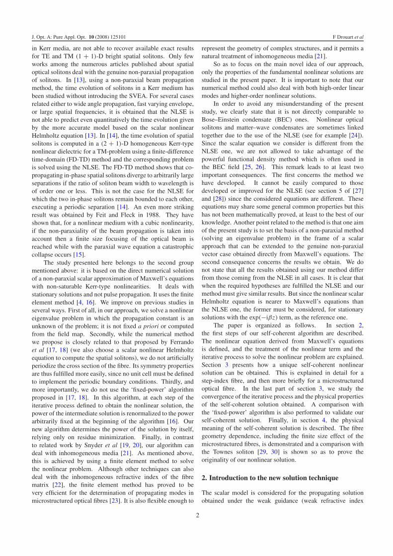
Figure 1. Logarithm of the residue obtained at the convergence,computed using the left-hand side of equation (9), versus the fieldamplitude χ0 for two different wavelengths and three different coreradii of the step-index fibre.

results with the well-established multipole method [1, 2] andwith the more recent fast Fourier factorization mode searchingmethod which is more versatile [22].

To correctly describe the field in the fibre and to minimizethe computation time, an adaptive mesh refinement is used:the stronger the field, the finer the mesh. In addition,the convergence of the SCLinN algorithm has been shownin [16], and in all the following tests we choose the prescribedtolerance δrelat

i < 10−10.

3.1. Scanning the amplitude of the linear initial field for thestep-index fibre

We start by studying the influence of the amplitude χ0 of theinitial (linear) field φr,0. For this, we inject χ0ψ0 at the firstiteration in the nonlinear term in equation (8):

�tψ1 + k20(n

20 + 1Inl|χ0ψ0|2)ψ1 − β2

1ψ1 = 0, (12)

in which the amplitude χ0 is arbitrarily fixed. Therefore, theinitialization of the SCLinN by a unique initial guess is replacedby a one-dimensional scan of the amplitude of the linear initialsolution. We denote this process the SCLin1D algorithm.

In addition, to start the study of SCLin1D , a cylindricalfibre with a Kerr material (nKerr = 3.2 × 10−20 m2 W−1) inthe circular core of radius 2.0 μm is considered. The linearpart of the refractive index of this core is n0 = 1.45. Thecore is embedded in an infinite cladding with a linear refractiveindex n = 1.435 (weak guidance approximation WGA). TheDirichlet condition at the edge of the geometry is also applied(in the present paper we do not address the computation of theleaky modes [1, 4]).

Figure 1 gives the effect of the initial field amplitude on theresidual values defined by the left-hand side of equation (9), fordifferent wavelengths and geometries.

Figure 1 shows the minimum residue for the nonlinearsolution at the convergence of the iterative process (i.e. whenδrelat

i < 10−10, the fixed point is reached). The influence of

4

J. Opt. A: Pure Appl. Opt. 10 (2008) 125101 F Drouart et al

(a) Final residue versus initial parameters

0 and 0 / lin.χ σ σ(b) Final residue versus final parameters

coh and coh / lin. (see the text for a complete description)χ σ σ

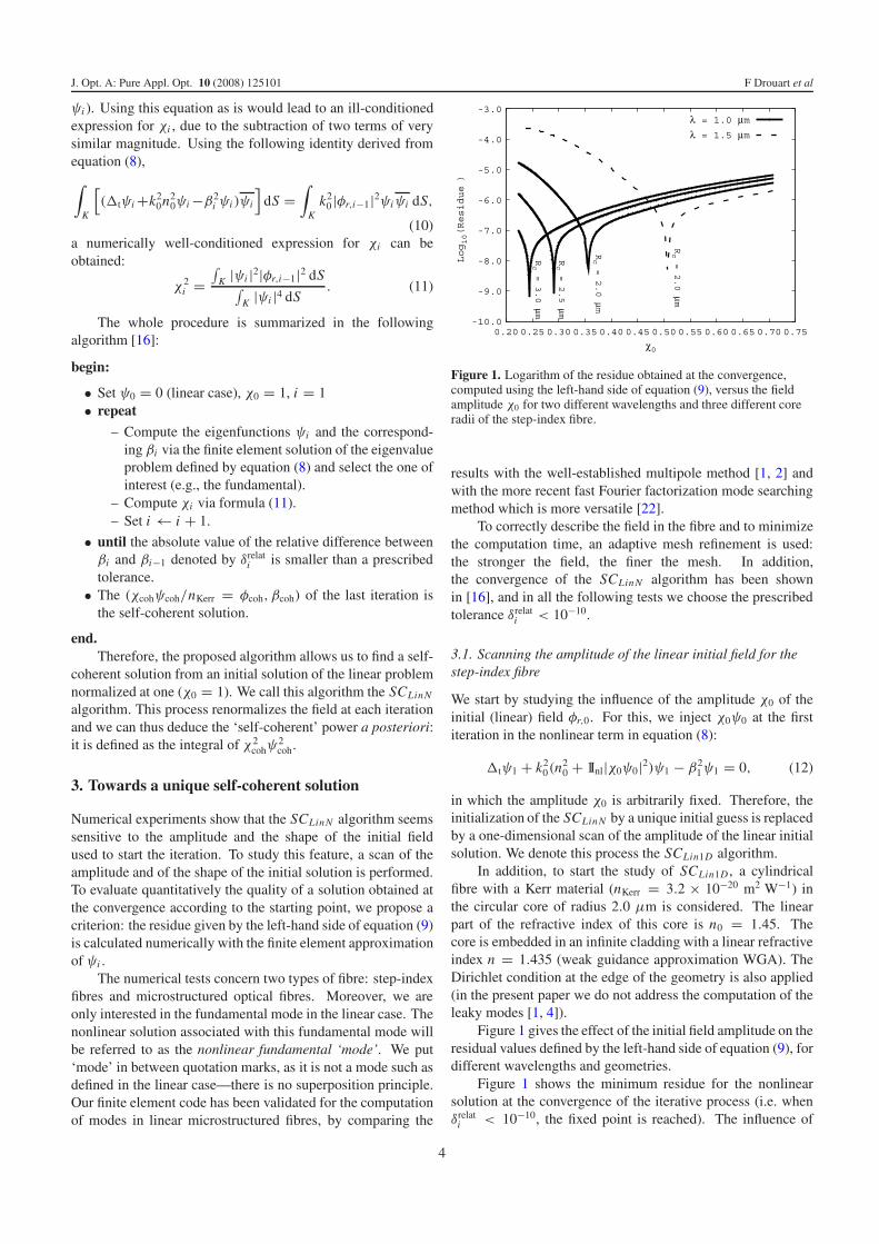
Figure 2. Maps of the residue computed for the nonlinear solution as a function of the input parameters characterizing the initial field (a) andas a function of the output parameters characterizing the nonlinear field (b) of the step-index fibre described in the text at λ = 1.0 μm.σlin corresponds to the standard deviation of the solution of the linear problem approximated by a Gaussian function.

the mesh has been ruled out by verifying that the minimumcorresponds to the same χ0 for different meshes. It maybe deduced that a single nonlinear solution is found foreach wavelength: it is the self-coherent nonlinear solution.Obviously there exists another minimum residue for χ0 = 0,corresponding to the solution of the linear problem.

3.2. Scanning both the amplitude and the width of the initialfield

In a further investigation, the residue is considered by scanningthe initial solution not only in amplitude but also in shape.At the first iteration, instead of the solution of the linearproblem, we inject a Gaussian function χ0e−(r/σ0)

2, where

r = √x2 + y2 and where σ0 represents the standard deviation

of the function. Therefore, the initialization of the SCLin1D

algorithm is replaced by a two-dimensional scan on χ0 and σ0.We call this process the SCGauss2D algorithm.

The computation is started with one value of σ0 andthe scan in χ0 is performed, then another value of σ0 istaken, and so on. Finally, the residue at the convergence ofSCGauss2D is obtained, according to the two parameters χ0 andσ0 characterizing the initial field, as shown in figure 2(a).

A narrow valley of minimal residues is observed. Thismeans that for one σ0 there exists a single χ0 such that one‘good’ final nonlinear solution is obtained: it is the self-coherent solution. Notice that the linear case corresponds toa vertical line in the figure 2(a) at σ0/σlin = 1 when theGaussian profile closely matches the profile of the fundamentalmode as in the WGA. Figure 2(a) suggests that there exists acontinuum of solutions depending on the value of σ0 given foreach minimum of the residue. Thus, the question is whetherthe nonlinear solutions obtained with the solution of the linearproblem or each Gaussian function (characterized by σ0) as thestarting point are the same: is the self-coherent solution reallyunique?

Figure 2(b) shows the absolute value of the logarithmof the residue according to the final solution parameters(χcoh, σcoh), in which we approximate this nonlinear solution

with a Gaussian fit. This figure shows that these finalparameters have nearly the same value. Therefore, from afull map of the initial parameters, the SCGauss2D algorithmprovides a localized surface formed by the final parameterscharacterizing the computed nonlinear solution. In addition,the minimum residues are localized in a small part of thissurface. These results allow us to confirm the assumptionthat the SCGauss2D algorithm finds a single nonlinear solution:the self-coherent nonlinear solution. This solution is a scalarspatial Kerr soliton in the step-index fibre.

Since for both studied cases (SCLin1D and SCGauss2D

algorithms) only a unique residue minimum associated to anonlinear solution (corresponding to the same β value) is foundfor all the step-index fibres and wavelengths we have tested,we can assume that this observed rule is general for this kindof fibres.

3.3. Results for the microstructured optical fibre

Microstructured optical fibres (MOFs) have more degrees offreedom related to the geometries and index contrasts thanstep-index fibres [4]. The study of these fibres allows us toextend the domain of validity of our algorithm and to compareour results with those previously published in [17]. The caseof a solid core MOF made of four rings of air holes embeddedin a Kerr material matrix (nKerr = 3.2 × 10−20 m2 W−1) isconsidered here. The linear part of the refractive index in thematrix is n0 = 1.45. The pitch � (space between the centre oftwo adjacent air hole centres) is equal to 10.0 μm and the airhole radius is equal to 2.75 μm.

As for the step-index fibre, the results obtained withSCLin1D show two minima for the residue: one associatedwith the solution of the linear problem (χ0 = 0) andone corresponding to the nonlinear solution. Whateverthe amplitude of the solution of the linear problem, asingle nonlinear solution—the self-coherent solution—is againfound.

For the SCGauss2D algorithm the Gaussian function isinjected only in the matrix and not in air holes since the

5

J. Opt. A: Pure Appl. Opt. 10 (2008) 125101 F Drouart et al

0 μ(a) (b) (c) (d)σ m=4 .0 0 =10.0 μσ m Final nonlinearfiled

Zoom on the center of the fibre

Figure 3. Field distribution in the microstructured optical fibre at λ = 5.0 μm for two initial Gaussian fields ((a) and (b)) and for thefundamental soliton ((c) and (d)).

field is usually very weak in the air holes due to the indexcontrast between the matrix and the inclusions. As for thestep-index fibre, there is a narrow valley (similar to that offigure 2(a)) corresponding to the minimal values of the residueas a function of the initial parameters χ0 and σ0/σlin. Themap of the final residue versus the final parameters χcoh andσcoh/σlin obtained is similar to that of figure 2(b).

Figure 3 shows the field distribution when the Gaussianfunction is used as an initial field, as well as the effectof the nonlinearity when SCGauss2D has converged. (Usingthe symmetry properties of the fibre, only a quarter of thegeometry needs to be modelled, which significantly reduces thecost of the numerical computations.) These figures illustratethe independence of the final self-coherent nonlinear solutionaccording to the spatial extent of the input initial field.

Therefore both for step-index fibres and for MOFs,SCLin1D and SCGauss2D lead to the same solution: the self-coherent solution. Actually, the most natural choice for thephysical studies is to use SCLin1D in which the starting pointdepends on the solution of the linear problem.

Note that a very fine scan must be performed to obtain theminimum value of the residue equal to the machine accuracy(10−15). Consequently, in practice, the speed and accuracyof the algorithm SCLin1D are improved by using the goldensection search in one dimension [34]. For each wavelengthstudied, the search is performed on the value of χ0. Thetypical shape of the function to be minimized is that in figure 1.Using this improvement, the algorithm is able to reach machineaccuracy for the minimal values of the computed residues.

3.4. Physical significance of the self-coherent solution:comparison with the ‘fixed-power’ method

A ‘fixed-power’ method was proposed by Ferrando et alin [17, 18] to find nonlinear solutions in MOFs with a Kerr termin the matrix refractive index. We call this process, in which thepower is given a priori, the algorithm F PFer . Our algorithmSCLinN can be easily modified (to study the ‘fixed-power’method) by replacing equation (11) with χ2

i = P/∫

K |ψi |2 dS,in which P is the fixed value of the power. We call our finiteelement method implementation of the ‘fixed-power’ processthe F PF E M algorithm.

To compare the physical properties of the solutions givenby F PFer , F PF E M , and SCLin1D , we use the quantities

0.0

0.2

0.4

0.6

0.8

1.0

1.2

1.4

1.6

1.8

2.0

0.0 0.2 0.4 0.6 0.8 1.0 1.2 1.4 1.6 1.8

Δ (x 10-3 )

γ (x 10-3)

a = 2.0

μma = 4.

0 μma = 6.

0 μma =

8.0 μm

a = 10.0 μm

γc = 1.7 x 10-3

Figure 4. Dependence of the gap function� on the nonlinearcoefficient γ for various air hole radii a at λ = 1.55 μm. Theseresults are obtained by using the algorithm F PF E M , and γc is definedin the text.

defined in [17]: the dimensionless nonlinear coefficient γ =Pn2

Kerr/A0 and the gap function� = (βNL −βlin)/k0, in whichP is the total power, and A0 = π(�/2)2 characterizes the coresize (for the step-index fibre, A0 = πR2

core, in which Rcore

is the radius of the core). βlin and βNL are the propagationconstants of the solution of the linear and nonlinear problems,respectively.

Our first study consists in comparing the results of thetwo implementations of the ‘fixed-power’ method: F PFer

and F PF E M . The computations are provided for a silicamicrostructured optical fibre with a pitch equal to 23.0 μm,for various air hole radii at λ = 1.55 μm [17]. TheMOF considered in F PF E M has a finite size and is madeof four rings of air holes, while the geometry for F PFer isperiodic. The evolution of the gap function � according to thenonlinear coefficient γ is computed (see figure 4) for variousair hole radii. This figure shows an approximate limit powercorresponding to γc = 1.7 × 10−3. As soon as γ > γc thenumerical process is divergent. Figure 4 shows that the valueof γc found with F PF E M is the same as that obtained withF PF E M (see figure 3(a) in [17]).

The second study consists in understanding the physicalsignificance of the self-coherent solution. To achieve this,

6

J. Opt. A: Pure Appl. Opt. 10 (2008) 125101 F Drouart et al

(a) Comparison for the step-index fibredescribed in section 3.1 at λ = 1.0 m and the corresponding residue

μ(b) Comparison for two MOFs with differentradii a at λ = 5.0 m and one associated residue for a =1.5 m

μμ

0.00 0.02 0.04 0.06 0.08 0.10–10.0

–9.0

–8.0

–7.0

–6.0

–5.0

Δ

Log10( Residue )

γ

Algorithm FPFEMAlgorithm SCLin1D

a = 1.

5 μm

a = 2.

75 μm

Residue(a = 1.5 μm)

0.00

0.01

0.02

0.03

0.04

0.05

Figure 5. Comparison between F PF E M and SCLin1D for the fundamental ‘mode’ for different fibres. γc corresponds to the critical power;above this value F PF E M diverges.

the physical powers obtained by F PF E M and SCLin1D arecompared. Therefore, this study consists in getting the valueof the ‘self-coherent power’ (i.e., Pcoh = ∫

F |χcoh|2|ψcoh|2 dS)obtained using SCLin1D . Then, the value of the physicalpower equal to Pphys. = Pcoh/n2

Kerr is deduced. Finally,some ascending values of power are injected as input inF PF E M until the value of the physical power Pphys. obtainedwith SCLin1D is reached. Figure 5 gives the results of thiscomparison for several fibres: the step-index one, figure 5(a),and two microstructured optical ones with different air holesizes, figure 5(b).

Figure 5(a) shows the comparison between F PF E M andSCLin1D for the step-index fibre described in section 3.1 at λ =1.0 μm. The ‘fixed-power’ algorithm F PF E M diverges forpower γ above the critical power γc (see figure 4). Contrary tothe results provided by F PFer in [17], the critical γ computedwith F PF E M depends slightly on the air hole radius a. As willbe shown in the next paragraph, this dependence is confirmedusing SCLin1D . This issue is also discussed in section 4.

The self-coherent algorithm SCLin1D finds the self-coherent solution at the corresponding critical power directly.As mentioned at the end of section 3.1, two minimal valuesof the residue are found. The first one corresponds to thelinear case γ = 0 and the second one corresponds to theself-coherent nonlinear solution. This solution is obtained bothwith SCLin1D and with SCGauss2D . The other solutions foundwith the ‘fixed-power’ method at lower powers are not the self-coherent solution because they do not correspond to a minimalresidue.

To complete this observation, the study is repeated forvarious MOFs (figure 5(b)). The computed results for thesetwo MOF geometries lead to the same conclusion as thatalready drawn for the step-index fibre: the self-coherentsolution obtained with the algorithm SCLin1D gives directly(and so, much more rapidly) the limit of the highest powersolution reachable (γ = γc) with the algorithm F PF E M .

Therefore, with our new SCLin1D algorithm and for eachfibre, a single self-coherent solution corresponding to thespatial soliton with the highest possible energy just before theself-focusing instability is easily obtained.

The last study is to compare the convergence of SCLin1D

with the one of the ‘fixed-power’ method F PF E M (figure 6).This figure shows the comparison of the convergence for

two different powers (represented by the γ coefficient) in theMOF described in section 3.3. Figure 6 proves that SCLin1D

converges much more rapidly than F PF E M . After 50 stepsthe convergence of F PF E M is not reached, whereas SCLin1D

requires 13 steps to converge. In addition, at the critical power(γ = γc), that is to say for the self-coherent solution, theeffective index cannot be found with F PF E M because thisalgorithm does not reach the required accuracy (for δrelat

i <

10−10) unlike the self-coherent algorithm SCLin1D .

4. Beyond the Townes soliton

As illustrated in figure 5, the self-coherent solutioncorresponds to the spatial soliton with the highest reachablepower before the self-focusing instability. Therefore, we canwonder whether this solution is the solution obtained for ahomogeneous silica medium with a nonlinear Kerr term [29].To analyse this issue, SCLin1D is implemented for this caseand the results are compared with those given by the followingfibre geometries (figure 7): the step-index fibres with variouscore radii in the case of the WGA described in section 3.1, anddifferent solid core microstructured optical fibres with variousair hole radii.

Figure 7 shows that the self-coherent solution of thenonlinear step-index fibre depends on the core radius. Thismeans that, even in the nonlinear case, the core/claddinginterface is important. The curves given in figure 7 alsoprove that the nonlinear solution obtained in the step-indexfibres differs from that of the homogeneous medium. As

7

J. Opt. A: Pure Appl. Opt. 10 (2008) 125101 F Drouart et al

1.430

1.440

1.450

1.460

1.470

1.480

0 10 20 30 40 50 60

neff=

β/k0

Number of steps

Algorithm FPFEM −γ = 0.086 < γc

Algorithm FPFEM

−γ = γc = 0.091Algorithm SC

Lin1D −γ = γc = 0.091

δ10relat = 2.9x10

–8

δ12relat = 5.1x10

–11

δ10relat = 2.7x10

–4

δ10relat = 4.8x10

–4

δ50relat = 2.9x10

–8

δ50relat = 1.3x10

–6

1.4748

1.4750

1.4752

1.4754

1.4756

1.4758

1.4760

1.4762

1.4764

1.4766

25 30 35 40 45 50 55

neff=

β/k0

Number of steps

Algorithm FPFEM

Algorithm SCLin1D

ZOOM

Figure 6. Convergence of SCLin1D compared with F PF E M for the fundamental ‘mode’ of the MOF described in section 3.3 at λ = 5.0 μm.δrelat

i is the absolute value of the relative difference between the values of β at the steps i − 1 and i . To make the comparison with the F PF E M

results easier, the value of neff for the self-coherent solution at step 13 of the SCLin1D is extended to step 50.

Figure 7. Comparison of the nonlinear effective index of the spatialsoliton versus the wavelength in different nonlinear waveguides andin a homogeneous nonlinear medium. The solid core MOFs studiedhave four rings of air holes with various radii a and� = 6.0 μm.The index contrast of the step-index fibres with various core radiifulfils the WGA.

expected, the higher the core radius (i.e. the structure tendsto the homogeneous medium), the smaller the difference withthe homogeneous medium. The same phenomenon is observedfor the MOFs, where the self-coherent solution does notcorrespond to that obtained in the homogeneous medium. Inaddition, the smaller the air hole radius (i.e. the structuretends to the homogeneous medium), the smaller the differencewith the homogeneous case. Figure 7 also shows that forsmaller wavelengths the role of the air holes decreases, theself-coherent solution being more confined. Notice that, inthe ‘fixed-power’ study [17], the ratio λ/� is small. Thisexplains the weak influence of the fibre geometry on thecritical nonlinear coefficient γc. As a consequence, the diagramof existence of spatial solitons (figure 3(b) in [17]) mustbe modified so as to take into account the influence of thewaveguide geometry. In the parameter space (γ, a) andusing the terminology defined in [17], the frontier between

the spatial soliton region and the self-focusing region is notexactly a vertical line defined by a unique critical nonlinearcoefficient γc. It is rather a line segment such that the lowerthe nonlinear coefficient the bigger the hole radius. The limitcase corresponds to a step-index fibre with nonlinear coresurrounded by an air ring with the hole diameter d = 2a =�/2 (see figure 7).

Therefore, the spatial solitons obtained with our algorithmfor nonlinear optical waveguides differ from that of a nonlinearhomogeneous medium.

The second point concerns the study of the Townessoliton [17, 29, 30]. The Townes soliton corresponds to thesolution of a propagation problem in a nonlinear homogeneousmedium. It corresponds to the critical solution before theself-focusing instability. We recall that the genuine Townessoliton, as defined in the seminal article written by Chiaoet al, is obtained without using the SVEA (see equations (5)and (6) in [29]) but the propagation constant of the solitonis computed from the field profile. The problem solved (seethe paragraph below equation (6) in [29]) is not an eigenvalueproblem. To assert the difference between our self-coherentsolution obtained for each structure with the Townes soliton,the power and the profiles of these solutions are studied. Thefirst step is to get the profile R(r) of the Townes soliton as thesolution of the one-dimensional (1D) equation:

�t R − R + R3 = 0, R′(0) = 0 and

R(∞) = 0. (13)

To solve this two-point boundary value problem a shootingmethod is used [34]. The profile of the solution is obtainedand shown in figure 1 of [29]. We have also calculated thecritical power coefficient Ncr [30] given by

Ncr =∫

�

|R|2r dr ≈ 1.862 (14)

where � corresponds to the 1D domain.To compare our self-coherent solution with the Townes

one, an expression of the self-coherent power Ncoh associated

8

J. Opt. A: Pure Appl. Opt. 10 (2008) 125101 F Drouart et al

with the critical power coefficient Ncr is defined. In physicalunits, the lower bound of the critical power P lb

cr is givenby [30, 33]

Ncr = 4πn0n2

λ2P lb

cr (15)

where n2 represents the nonlinear coefficient characterizing theKerr medium. The scalar optical Kerr effect can be definedas follows: εr(φ) = (n0 + n2|φ|2)2 ≈ n2

0 + 2n0n2|φ|2, andwe have defined n2

Kerr = 2n0n2, in which n2 is the nonlinearcoefficient characterizing the material [5]. However, in ourcase, an eigenvalue-like problem is solved. Indeed, unlike theTownes soliton studies [29, 30], the propagation constant βis considered so as to describe completely the features of thenonlinear self-coherent solution. To take into account the βcoh

eigenvalue of our approach, the physical power Pphys defineddirectly from the Poynting theorem is calculated. In this case,

Pphys = βcoh

k0

P lbcr = Pcoh

n2Kerr

= Pcoh

2n0n2, (16)

in which Pcoh = ∫�

|χcoh|2|ψcoh|2 dS is the self-coherent powerobtained at the convergence of SCLin1D , and k0 = 2πn0/λ isdefined so as to compare with the critical power coefficient Ncr

given in [30]. Consequently, we get

P lbcr = k0

2n0n2βcohPcoh. (17)

Therefore, the coefficient Ncoh permitting us to compareour scalar spatial Kerr solitons with the Townes soliton can bedefined, by using P lb

cr of the equation (17) in expression (15),as

Ncoh = 4π2n0

βcohλ3Pcoh. (18)

Figure 8 shows the comparison between the coefficientNcoh for step-index fibres with various core radii, for solid coreMOFs with various air hole sizes, and for the homogeneousmedium with the critical power coefficient Ncr of the Townessoliton. These results confirm those obtained in figure 7, andthey illustrate the influence of the fibre geometry. In addition,figure 8 shows that the smaller the wavelength (the field is moreconfined in the MOF core), the smaller the difference betweenthe Townes soliton and the self-coherent solutions.

Figure 8 also gives the evolution of the value of Ncoh in thehomogeneous medium case, with respect to the wavelength. Asexplained above, our numerical approach SCLin1D takes intoaccount the β value. Nevertheless, it is very near the constantone of the genuine Townes soliton (1.4555 instead of 1.45). Amore detailed wavelength dependence cannot be obtained withthe current numerical accuracy of the effective indices. We canrecall that it is known from the seminal work of Chiao et althat for the Townes soliton this dependence is really weak (seepage 480 of [29], second column).

It is interesting to notice that the nonlinear self-coherentsolution (obtained with SCLin1D from equation (6), φ and βbeing unknown) in the homogeneous medium corresponds wellto the Townes soliton (obtained from equation (13) with ashooting method).

Figure 8. Evolution of the value of the self-coherent powercoefficient Ncoh for various step-index fibres, for different solid coreMOFs, and for the homogeneous medium as a function of thewavelength. The horizontal dashed line is the critical powercoefficient Ncr = 1.862 of the Townes soliton.

Figure 9 illustrates the dependence of the nonlinear self-coherent profile as a function of the wavelength and of thefibre geometry. The global shapes of these spatial solitonsare similar that of the Townes soliton (see figure 1 in [29] andfigure 1 in [30] that show clearly that the Townes soliton canbe approximated with a Gaussian curve) but the amplitudes aredifferent. As expected at a fixed wavelength, the spatial widthof these spatial solitons decreases with the radius a of the airholes but the maximal amplitude increases. Nevertheless, theratio Pcoh/βcoh which appears in formula (18) decreases witha, inducing an overall decrease of the critical power coefficientNcoh (see also figure 8).

The next point concerns the influence of the finite size ofthe structure. The solid core MOF considered in figure 10 hasthe same geometry as that described in section 3.3 but the airhole radius is equal to 1.0 μm. The results are given for severalnumbers of air hole rings Nr . As can be seen in figure 10, thecurve order is reversed between the linear and the nonlinearcases for the MOFs.

In the linear case and at a fixed wavelength, the effectiveindex increases when Nr increases, which is well known [4]. Inthe nonlinear case, the evolution of Nr is physically coherentwith the wavelength dependence already observed in figure 7:the more the structure confines the field, the lower is thenonlinear effective index. Obviously, if the air hole radiusincreases, the influence of the finite size structure becomesnegligible. These results prove that the nonlinear self-coherentsolution depends not only on the MOF structure but also on itsfinite size.

Last, figure 11(a) gives the evolution of the linear andnonlinear effective indices and normalized effective area versusthe wavelength obtained with SCLin1D for a step-index fibredescribed in section 3.1.

Figure 11(a) shows that the larger the wavelength, thestronger the nonlinear effect. To confirm this observation,figure 11(b) shows that the effective area obtained in thenonlinear case is constant in comparison with the linear case.

9

J. Opt. A: Pure Appl. Opt. 10 (2008) 125101 F Drouart et al

(a) λ =3.5 mμ (b) λ =10.0 mμ

Figure 9. Field profiles for three MOFs with four air hole rings at two wavelengths. The coloured region represents the first air hole of theMOF according to the radius and the associated values of the ‘self-coherent power’.

Figure 10. Effect of the number of air hole rings Nr in a solid coreMOF (� = 6.0 μm and a = 1.0 μm) on the effective indexaccording to the wavelength in the linear and nonlinear cases.

Thus, the field scattering which increases with the wavelengthis challenged by the nonlinear effect.

From the results of this section, we can infer thatdifferences from Townes soliton properties will be observedin waveguides in which the ratio of the wavelength over thecharacteristic size of the nonlinear core is above a constantslightly smaller that unity. Such a ratio is only three times thatmeasured in a nonlinear glass planar waveguide [35] and canbe overcome in structures like nanowires [36].

5. Discussion

The self-coherent algorithm SCLin1D has been presented forthe scalar approach within the weak guidance approximation.Neglecting the term ∇[E · ∇εr/εr], we obtain the equation�E + k2

0εrE = 0. However, for the step-index fibre, while theweak index contrast is fulfilled in the linear case, as soon aswe have considered the Kerr effect the index contrast increases

and the WGA is not valid any more (see figure 12(a)). Forthe microstructured optical fibre, even the linear case does notobey this approximation (see figure 12(b)). Indeed, the WGAis only validated if the relative index variation is negligibleon a distance of one wavelength [31]. Consequently, so asto obtain more accurate results, future studies must deal withthe full vector problem. Such an extension of the presentwork is possible since our original numerical method can beformulated in the vector case [4, 23].

The second issue is the value of the physical powerPphys. = Pcoh/n2

Kerr of the nonlinear self-coherent solution.This implies that the stronger the Kerr coefficient n2 (orn2

Kerr = 2n0n2), the weaker the physical power. Nevertheless,even if we choose chalcogenide glasses which are known tohave a high Kerr nonlinearity [37, 38], the power of the self-coherent solution is huge as already computed for the Townessoliton power [29]. With n2

Kerr = 10−17 m2 W−1, one gets asoliton power of 2.6 × 104 W at 2 μm for the MOF describedin section 3.3 and 7.4 × 105 W at 10 μm. These resultssuggest that the scalar self-coherent solution cannot easily bevalidated by experiments. In the scalar approach used in ourstudy, from a practical point of view the induced increasein the refractive index of the core or of the matrix is soimportant that either other nonlinear effects should be takeninto account or the medium is damaged [39]. However, spatialoptical solitons have already been observed in planar nonlinearglass waveguides using a 4 × 105 W input at 620 nm using75 fs pulses [35]. It will be interesting to know if, in thevector case, the physical power of the self-coherent soliton willdecrease or not so as to make it more accessible to experimentalobservation.

The third issue of the discussion concerns the stabilityof the self-coherent solutions. This is a difficult problemsince, in the present cases, it requires one to solve a 3Dpropagation problem along the waveguide axis. For the fixed-power solutions, Ferrando et al [17] have already proved thatthe spatial solitons are stable under arbitrary perturbations.They also showed that spatial solitons found at fixed power

10

J. Opt. A: Pure Appl. Opt. 10 (2008) 125101 F Drouart et al

(a) Evolution of the effective indices (b) Evolution of the effective area normalizedwith the core area A0 = R 2

coreπ

Figure 11. Evolution of the linear and nonlinear effective indices and normalized effective area versus the wavelength for the step-index fibredescribed in section 3.1. For the nonlinear case, the SCLin1D algorithm is used.

(a) Refractive index profile for the step-index fibre at λ = 1.0 m (see section 3.1 for a complete description of the structure)

μ(b) Refractive index profile according to thehorizontal axis of the microstructured fibre at λ = 5.0 m (see section 3.3 for a complete description of the structure)

μ

Figure 12. Effective index profile computed from equation (3) in the linear and nonlinear case for the fundamental ‘mode’ of the two fibretypes described in the text.

are stable under both small transverse displacements relativeto the hole cladding and non-perfect launching conditions. Inthe case of the self-coherent spatial solitons described in thepresent article, a stability analysis should also be performed.Although this issue is crucial in the case of nonlinear studies,it is beyond the scope of this initial work.

The last issue concerns the comparison with NLSEstudies, as already mentioned in section 1. The counterpartof our non-paraxial description of spatial solitons is thatthe results we obtain are less general than the NLSE oneswhich can be related to both nonlinear optics and Bose–Einstein condensates [24]. Our results are not obtainedwith the powerful methods coming from quantum mechanics(like functional density approach) [25, 26] but with a more

numerical method well adapted to our non-paraxial problem.Nevertheless, as long as stationary states are considered, ourapproach, which considers the nonlinear Helmholtz equationas an eigenvalue problem (with the propagation constant asan unknown), is a better model of Maxwell’s equations in anonlinear Kerr-type medium.

6. Conclusions

We have demonstrated that the nonlinear self-coherent solutionfound in step-index fibres and solid core MOFs, correspondingto the spatial soliton with the highest reachable energy avoidingthe self-focusing instability, is different from the Townessoliton. This solution generalizes the Townes soliton within

11

J. Opt. A: Pure Appl. Opt. 10 (2008) 125101 F Drouart et al

finite size waveguides. This result, built in the frame of a non-paraxial and scalar approach for stationary solutions, relies ona new algorithm implemented using the finite element method.

To find the nonlinear self-coherent solution, two distinctcriteria are defined: the convergence of the algorithm tothe required accuracy (the fixed point) and the minimumof the residue at this point. By solving the eigenvalueproblem, a single nonlinear solution verifying these criteria isfound, for given wavelength and fibre geometry. This singlesolution of the eigenvalue problem is obtained with variousinitial guesses: the solution of the associated linear problem(SCLin1D algorithm) and some Gaussian functions (SCGauss2D

algorithm).So as to verify the numerical results obtained with the

self-coherent algorithm SCLin1D , several comparisons havebeen performed. We can adapt our numerical method toobtain a ‘fixed-power’ algorithm denoted F PF E M . The resultscomputed with F PF E M are in good agreement with alreadypublished data for MOFs given in [17], called here F PFer .The comparison between F PF E M and SCLin1D has shown thatthe self-coherent solution is obtained at the critical power justbefore the self-focusing instability. The SCLin1D algorithm isshown to be more reliable and more efficient than F PF E M tofind the critical power of the spatial solitons.

Then, the physical meaning of the self-coherent nonlinearsolution of a step-index fibre with a Kerr material core and ofsolid core MOFs with Kerr material matrix is discussed. Twocomparisons are made: one with the self-coherent solutioncomputed for a homogeneous Kerr material and the secondone with the usual Townes soliton computed for the samestructure. From the mathematical point of view the formerproblem is a nonlinear eigenvalue problem while the latter isa two-point boundary value problem (since the dependenceon the propagation is not taken into account.) We haveshown that the self-coherent spatial solitons found for thestep-index fibres and for MOFs are different from those ofthe homogeneous nonlinear medium and from the genuineTownes soliton. In the various structures considered in thepresent paper, the dependence of the self-coherent solutions isdescribed as a function of the wavelength. We have observedthat, as expected, these self-coherent spatial solitons convergetowards the Townes soliton at small wavelengths. We havealso observed that the amplitude of the nonlinear self-coherentsolution depends on the waveguide geometry: the core size forthe step-index fibre, and the air hole radius and number of airhole rings for the solid core MOFs.

Finally, the study of the refractive index induced by thenonlinear self-coherent solution has been performed. The weakguidance approximation and the scalar model are no longervalid if the self-coherent solution is considered. To tackle thisproblem, a study of the full-vectorial version of the proposedmethod, including a study of the losses, is under development.

Acknowledgments

We would like to thank Gadi Fibich and Yonatan Sivan fromthe Department of Applied Mathematics of Tel Aviv Universityfor their help concerning the study of the Townes solitonprofile.

References

[1] Kuhlmey B, White T P, Renversez G, Maystre D, Botten L C,de Sterke C M and McPhedran R C 2002 Multipole methodfor microstructured optical fibers II: implementation andresults J. Opt. Soc. Am. B 10 2331–40

[2] Kuhlmey B, Renversez G and Maystre D 2003 Chromaticdispersion and losses of microstructured optical fibersAppl. Opt. 42 634–9

[3] Renversez G, Bordas F and Kuhlmey B T 2005 Second modetransition in microstructured optical fibers: determination ofthe critical geometrical parameter and study of the matrixrefractive index and effects of cladding size Opt. Lett.30 1264–6

[4] Zolla F, Renversez G, Nicolet A, Kuhlmey B, Guenneau S andFelbacq D 2005 Foundations of Photonic Crystal Fibres(London: Imperial College Press)

[5] Agrawal G P 2001 Nonlinear Fiber Optics 3rd edn (New York:Academic)

[6] Kivshar Y S and Agrawal G P 2003 Optical Solitons(Amsterdam: Academic)

[7] Chen Y and Atai J 1997 Maxwell’s equations and the vectornonlinear Schrodinger equation Phys. Rev. E 55 3652–7

[8] Akhmediev N, Ankiewicz A and Soto-Crespo J M 1993 Doesthe nonlinear Schrodinger equation correctly describe beampropagation? Opt. Lett. 18 411

[9] Ciattoni A, Crossignani B, Di Porto P and Yariv A 2005 Perfectoptical solitons: spatial Kerr solitons as exact solutions ofMaxwell’s equations J. Opt. Soc. Am. B 22 1384–94

[10] Karlsson M, Anderson D, Desaix M and Lisak M 1991Dynamic effects of Kerr nonlinearity and spatial diffractionon self-phase modulation of optical pulses Opt. Lett.16 1373

[11] Karlsson M, Anderson D and Desaix M 1992 Dynamics ofself-focusing and self-phase modulation in a parabolic indexoptical fiber Opt. Lett. 17 22

[12] Ciattoni A, Crossignani B, Di Porto P, Scheuer J andYariv A 2006 On the limit of validity of nonparaxialpropagation equations in Kerr media Opt. Express14 5517–23

[13] Selleri S, Vincenti L and Cucinotta A 1998 Finite elementmethod resolution of non-linear Helmholtz equationOpt. Quantum Electron. 30 457–65

[14] Joseph R M and Taflove A 1994 Spatial soliton deflectionmechanism indicated by FD-TD Maxwell’s equationsmodeling IEEE Photon. Technol. Lett. 6 1251–4

[15] Feit M D and Fleck J A Jr 1988 Beam nonparaxiality, filamentformation, and beam breakup in the self-focusing of opticalbeams J. Opt. Soc. Am. B 5 633

[16] Nicolet A, Drouart F, Renversez G and Geuzaine C 2007A finite element analysis of spatial solitons in optical fibresCOMPEL 26 1105–13

[17] Ferrando A, Zacares M, Fernandez de Cordoba P, Binosi D andMonsoriu J A 2003 Spatial soliton formation in photoniccrystal fibers Opt. Express 11 452–9

[18] Ferrando A, Zacares M, Fernandez de Cordoba P andMonsoriu J A 2004 Vortex solitons in photonic crystal fibersOpt. Lett. 12 817–22

[19] Snyder A W, Mitchell D J and Chen Y 1994 Spatial solitonsof Maxwell’s equations Opt. Lett. 19 524–6

[20] Snyder A W, Hewlett S J and Mitchel D J 1994 Dynamicspatial solitons Phys. Rev. Lett. 72 1012–5

[21] Nicolet A, Guenneau S and Zolla F 2004 Modelling of twistedoptical waveguides with edge elements Eur. Phys. J. Appl.Phys. 28 153–7

[22] Boyer P, Renversez G, Popov E and Neviere M 2007 Improveddifferential method for microstructured optical fibres J. Opt.A: Pure Appl. Opt. 9 728–40

12

J. Opt. A: Pure Appl. Opt. 10 (2008) 125101 F Drouart et al

[23] Guenneau S, Nicolet A, Zolla F and Lasquellec S 2002Modeling of photonic crystal fibers with finite elementsIEEE Trans. Magn. 38 1261–4

[24] Alexander T J and Berge L 2002 Ground states and vortices ofmatter–wave condensates and optical guided wavesPhys. Rev. E 65 026611

[25] Dalfovo F, Renversez G and Treiner J 1992 Vortices with morethan one quantum of circulation in He-4 at negative-pressureJ. Low Temp. Phys. 89 425–8

[26] Dalfovo F, Giorgini S, Pitaevskii L P and Stringari S 1999Theory of Bose–Einstein condensation in trapped gasesRev. Mod. Phys. 71 463–512

[27] Garcıa-Ripoll J J and Perez-Garcıa V M 2001 OptimizingSchrodinger functionals using Sobolev gradients:applications to quantum mechanics and nonlinear opticsSIAM J. Sci. Comput. 23 1315–33

[28] Ablowitz M J, Ilan B, Schonbrun E and Piestun R 2006 Solitonsin two-dimensional lattices possessing defects, dislocations,and quasicrystal structures Phys. Rev. E 74 035601

[29] Chiao R Y, Garmire E and Townes C H 1964 Self-trapping ofoptical beams Phys. Rev. Lett. 13 479–82

[30] Fibich G and Gaeta A L 2000 Critical power for self-focusingin bulk media and in hollow waveguides Opt. Lett. 25 335–7

[31] Marcuse D 1991 Theory of Dielectric Optical Waveguides2nd edn (San Diego, CA: Academic)

[32] Snyder A W and Love J D 1983 Optical Waveguide Theory(New York: Chapman and Hall)

[33] Boyd R W 2003 Nonlinear Optics 2 edn (New York:Academic)

[34] Press W H, Flannery B P, Teukolsky S A and Vetterling W T1986 Numerical Recipes (Cambridge: Cambridge UniversityPress)

[35] Aitchison J S, Weiner A M, Silberberg Y, Oliver M K,Jackel J L, Leaird D E, Vogel E M and Smith P W E 1990Observation of spatial optical solitons in a nonlinear glasswaveguide Opt. Lett. 15 471–3

[36] El-Ganainy R, Mokhov S, Makris K G, Christodoulides D Nand Morandotti R 2006 Solitons in dispersion-invertedAlGaAs nanowires Opt. Express 14 2277–82

[37] Smektala F, Quemard C, Couderc V and Barthelemy A 2000Non-linear optical properties of chalcogenide glassesmeasured by z-scan J. Non-Cryst. Solids 274 232–7

[38] Brilland L, Smektala F, Renversez G, Chartier T, Troles J,Nguyen T, Traynor N and Monteville A 2006 Fabrication ofcomplex structures of holey fibers in chalcogenide glassOpt. Express 14 1280–5

[39] Stuart B C, Feit M D, Rubenchik A M, Shore B W andPerry M D 1995 Laser-induced damage in dielectrics withnanosecond to subpicosecond pulses Phys. Rev. Lett.12 2248–51

13