arX

iv:1

801.

0289

4v1

[cs

.IT

] 9

Jan

201

81

Spatial Lattice Modulation for MIMO Systems

Jiwook Choi, Yunseo Nam, and Namyoon Lee

Abstract

This paper proposes spatial lattice modulation (SLM), a spatial modulation method for multiple-

input-multiple-output (MIMO) systems. The key idea of SLM is to jointly exploit spatial, in-phase, and

quadrature dimensions to modulate information bits into a multi-dimensional signal set that consists of

lattice points. One major finding is that SLM achieves a higher spectral efficiency than the existing spatial

modulation and spatial multiplexing methods for the MIMO channel under the constraint of M -ary pulse-

amplitude-modulation (PAM) input signaling per dimension. In particular, it is shown that when the SLM

signal set is constructed by using dense lattices, a significant signal-to-noise-ratio (SNR) gain, i.e., a

nominal coding gain, is attainable compared to the existing methods. In addition, closed-form expressions

for both the average mutual information and average symbol-vector-error-probability (ASVEP) of generic

SLM are derived under Rayleigh-fading environments. To reduce detection complexity, a low-complexity

detection method for SLM, which is referred to as lattice sphere decoding, is developed by exploiting

lattice theory. Simulation results verify the accuracy of the conducted analysis and demonstrate that

the proposed SLM techniques achieve higher average mutual information and lower ASVEP than do

existing methods.

Index Terms

Multiple-input-multiple-output (MIMO), spatial modulation (SM), lattice modulation.

I. INTRODUCTION

Spatial modulation (SM) [1] is a transmission method that sends information bits using the

index of an active antenna and conventional quadrature-amplitude-modulation (QAM) symbols.

SM has been proposed to improve both the spectral and energy efficiency of MIMO systems

[2]–[5]. For example, when a transmitter is equipped with Nt antennas that use a radio frequency

J. Choi, Y. Nam, and N. Lee are with the department of electrical engineering, POSTECH, South Korea,

emails:{jiwook,edwin624,nylee}@postech.ac.kr

2

(RF) chain, log2 (Nt) + log2(|CQ|) bits can be modulated into a spatial symbol vector, where CQdenotes the QAM constellation set and |CQ| represents its cardinality. A simplified version of

SM, referred to as space shift keying (SSK) [6] was presented to improve energy efficiency. SSK

only maps information bits into the antenna index, so it is able to achieve the spectral efficiency

of log2 (Nt) bits/sec/Hz when signal-to-noise ratio (SNR) is high enough.

The concepts of SM and SSK have been generalized in numerous ways by mapping informa-

tion bits into multiple indices of the transmit antennas. Generalized spatial modulation (GSM)

[7] and generalized space shift keying (GSSK) [8] are representative generalizations of SM. The

idea of both GSM and GSSK is to map information bits onto an antenna subset that consists

of Na elements among Nt. Therefore, a transmitter is able to modulate log2(Nt

Na

)+ log2(|CQ|)

information bits when using GSM with constellation set CQ. This modulation strategy allows

sending of log2(Nt

Na

)− log2

(Nt

1

)more information bits than both SM and SSK. Multiple active

spatial modulation (MA-SM) [9] is another variation of GSM, MA-SM was introduced by

harnessing multiplexing gains of the MIMO system. MA-SM sends distinct QAM symbols by

choosing Na active elements among Nt transmit antennas; thereby, log2(Nt

Na

)+ Na log2(|CQ|)

information bits are modulated to a symbol vector with QAM constellation set CQ.

Variable set of active antenna GSM (VA-GSM) [10] is another variation of GSM. VA-GSM

allows the number of active antennas to vary from 1 to Nt, while sending the same transmit

symbol for each active antenna. In addition, quadrature spatial modulation (QSM) [11] separately

exploits in-phase and quadrature signal dimensions. For instance, when a transmitter has Nt

antennas, QSM is able to modulate 2 log2 (Nt) + log2 (|CQ|) information bits. Recently, another

generalized method of GSM, called GSM with multiplexing (GSMM) [12], was introduced.

GSMM sends S data symbols using a set of precoding matrices F in which 1 ≤ S ≤ Nt and

|F| = 2Nt −1. As a result, GSMM is able to modulate log2(2Nt − 1

)+S log2(|CQ|) information

bits. The common limitation of the methods in [7]–[12] is that information bits are separately

modulated to the index of active antenna-subsets (or the index of precoding matrices [12]) and to

the transmission of QAM symbols. This separated modulation approach generally cannot achieve

a higher spectral efficiency than that attained by a joint modulation strategy for a fixed Nt and

CQ.

Adaptive-joint-mapping GSM (AJM-GSM) [13] and jointly-mapped SM (JM-SM) [14] both

jointly modulate information bits into an active antenna index and transmit symbols using the

proposed joint mapping rule. This joint mapping can generate more signal points than the

3

mapping methods that separately modulate information bits into the indices of antenna subsets

and transmit symbols. The limitation of the methods in [11] and [14] is that they do not jointly

take into account all possible signaling dimensions, (i.e., spatial, in-phase, quadrature) when

constructing signal sets for SM.

Since the minimum Euclidean distance between adjacent symbols in a constellation set affects

the detection accuracy, numerous methods for the signal set design of SM have been proposed

to maximize the minimum distance [15]–[17]. For instance, the QAM symbols of MA-SM [9]

are rotated to a different phase for each active antenna-subset; as a result, the minimum distance

increases. Enhanced spatial modulation (ESM) [15], [16] uses a similar approach. The idea of

ESM is to construct a primary and a secondary signal constellation set. Then the secondary set

is interpolated into the primary set to increase the minimum distance between symbol vectors.

Another constellation design method for SM exploits Eisenstein integer [17]; in this method, a

transmitter uses a two-dimensional hexagonal lattice to send symbols. This lattice is the densest

packing lattice in a two-dimensional complex domain. All these methods [15]–[17] demonstrate

that carefully-designed constellation sets is able to achieve higher SNR gains than SM methods

that use the conventional QAM constellation set.

In this paper, we consider a MIMO system in which a transmitter is equipped with Nt transmit

antennas and a receiver is equipped with Nr receive antennas. We assume that the transmitter

can send one symbol per in-phase (or quadrature) component of each transmit antenna from the

M-ary pulse-amplitude-modulation (PAM) signal set C ={−M

2, −M

2+ 1, . . . , M

2− 1, M

2

}. The

contributions of this paper are summarized as follows:

• Our major contribution is to propose a novel multidimensional spatial modulation method

called spatial lattice modulation (SLM). Unlike the existing SM techniques in which in-

formation bits are separately mapped to a set of antenna indices and modulation symbols

[7]–[10], [12], the key idea of the proposed SLM is to modulate information bits into a

set of lattice points in R2Nt by jointly exploiting spatial, in-phase, and quadrature signal

dimensions. An element of each lattice point is chosen from the set C = {0} ∪ C with

|C| = M + 1, where the null element {0} indicates that the input signal for a chosen

signal dimension is deactivated for SM. In particular, we present two SLM methods: SLM

using a simple cubic lattice and SLM that uses a dense packing lattice that has a large

nominal coding gain in a low-dimensional vector space [18], [19]. We show that the

proposed SLM methods achieve the spectral efficiency of 2Nt log2 (M + 1) bits/sec/Hz

4

when SNR is high enough. This result is interesting because it enables the transmission

of 2Nt (log2 (M + 1)− log2 (M)) additional information bits per channel use compared to

the conventional spatial multiplexing; this gain is unbounded as Nt increases. In particular,

to attain a nominal coding gain for a given target spectral efficiency, we propose a signal

set design algorithm that uses Barnes-Wall lattices for SLM; these are the densest lattices

below 16 dimensions (or eight transmit antennas).

• We also analyze the average mutual information and average symbol-vector-error-probability

(ASVEP) of the proposed SLM methods under a Rayleigh MIMO channel. Although the

mutual information expressions have been characterized for SM and GSM in [21]–[23] for

a fixed MIMO channel, the average mutual information expression is unknown for general

SM methods. We derive a tight approximation of the average mutual information in a

closed-form for the proposed SLM methods. We also derive a closed-form upper bound of

ASVEP for SLM to complete our analysis. Simulation results verify the effectiveness of

our analysis. One major observation is that SLM using dense lattices provides SNR gains

in both the average mutual information and the ASVEP.

• Lastly, we present a low-complexity SLM detection method, which is called lattice sphere

decoding (LSD). The key idea of LSD is to exploit the property that a lattice is closed under

addition. Using this lattice property, the proposed LSD algorithm reduces the effective search

space of SLM by calculating ML metrics only in the closest lattice vectors from an initially

estimated lattice vector. We show that the complexity order of the proposed LSD algorithm

is O (N3t ), which is the same detection complexity order with linear-type detection methods

such as zero-forcing MIMO detection. Simulation results show that the error performance of

LSD closely matches that of ML detection in practical MIMO systems, while significantly

diminishing the detection complexity.

II. SYSTEM MODEL AND PRELIMINARYIES

This section presents the system model considered in this paper and provides some useful

mathematical definitions that will be used subsequently.

A. System Model

We consider a MIMO channel in which a transmitter equipped with Nt transmit antennas sends

information symbols to a receiver equipped with Nr receive antennas. We denote the complex

5

Information bits, , ,

Spatial LatticeMapper

Re

Im

RF chain

Tx #1

Tx #Encoder

Re

Im

RF chain

Spatial Lattice Modulator Rx #1

Rx #

RF chain

RF chain

Re

Im

Re

Im

Spatial LatticeDemapper decoder

Spatial Lattice Demodulator

Information bits

, , ,

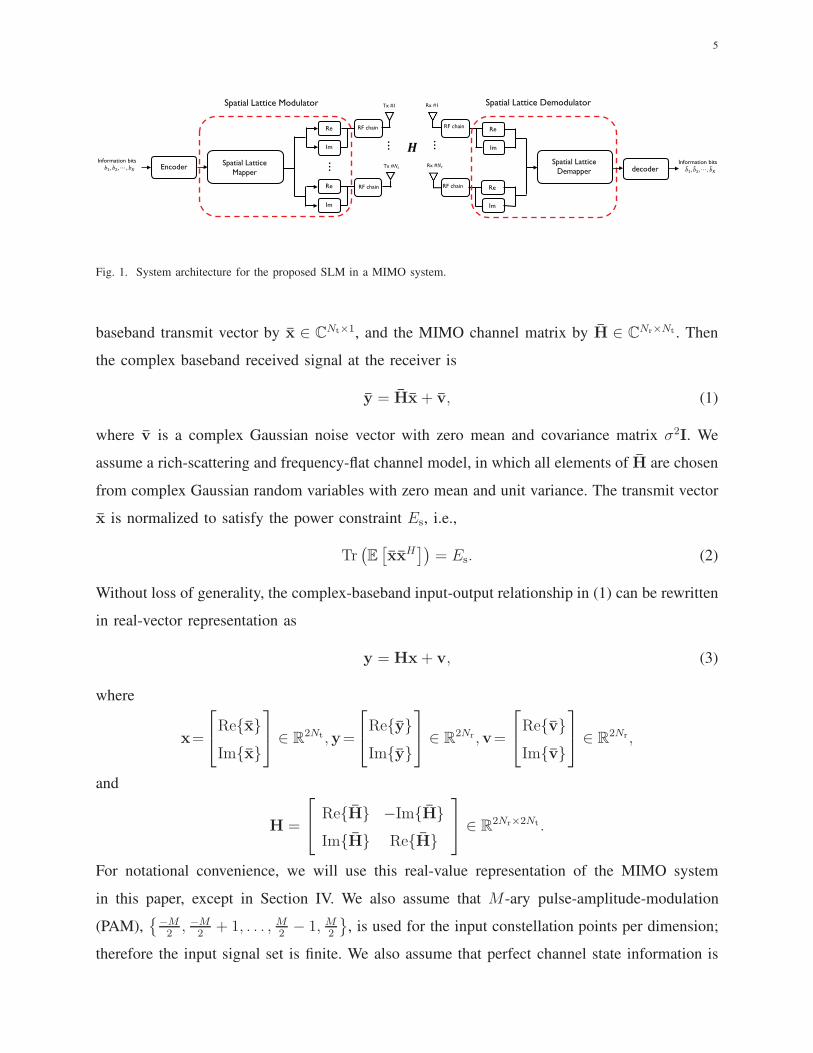
Fig. 1. System architecture for the proposed SLM in a MIMO system.

baseband transmit vector by x ∈ CNt×1, and the MIMO channel matrix by H ∈ CNr×Nt . Then

the complex baseband received signal at the receiver is

y = Hx + v, (1)

where v is a complex Gaussian noise vector with zero mean and covariance matrix σ2I. We

assume a rich-scattering and frequency-flat channel model, in which all elements of H are chosen

from complex Gaussian random variables with zero mean and unit variance. The transmit vector

x is normalized to satisfy the power constraint Es, i.e.,

Tr(E[xxH

])= Es. (2)

Without loss of generality, the complex-baseband input-output relationship in (1) can be rewritten

in real-vector representation as

y = Hx+ v, (3)

where

x=

Re{x}Im{x}

∈ R2Nt ,y=

Re{y}Im{y}

∈ R2Nr ,v=

Re{v}Im{v}

∈ R2Nr,

and

H =

Re{H} −Im{H}Im{H} Re{H}

∈ R2Nr×2Nt .

For notational convenience, we will use this real-value representation of the MIMO system

in this paper, except in Section IV. We also assume that M-ary pulse-amplitude-modulation

(PAM),{−M

2, −M

2+ 1, . . . , M

2− 1, M

2

}, is used for the input constellation points per dimension;

therefore the input signal set is finite. We also assume that perfect channel state information is

6

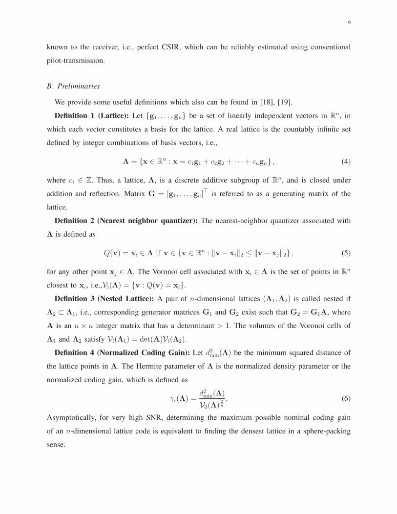
known to the receiver, i.e., perfect CSIR, which can be reliably estimated using conventional

pilot-transmission.

B. Preliminaries

We provide some useful definitions which also can be found in [18], [19].

Definition 1 (Lattice): Let {g1, . . . , gn} be a set of linearly independent vectors in Rn, in

which each vector constitutes a basis for the lattice. A real lattice is the countably infinite set

defined by integer combinations of basis vectors, i.e.,

Λ = {x ∈ Rn : x = c1g1 + c2g2 + · · ·+ cngn} , (4)

where ci ∈ Z. Thus, a lattice, Λ, is a discrete additive subgroup of Rn, and is closed under

addition and reflection. Matrix G = [g1, . . . , gn]⊤

is referred to as a generating matrix of the

lattice.

Definition 2 (Nearest neighbor quantizer): The nearest-neighbor quantizer associated with

Λ is defined as

Q(v) = xi ∈ Λ if v ∈ {v ∈ Rn : ‖v − xi‖2 ≤ ‖v− xj‖2} , (5)

for any other point xj ∈ Λ. The Voronoi cell associated with xi ∈ Λ is the set of points in Rn

closest to xi, i.e.,Vi(Λ) = {v : Q(v) = xi}.

Definition 3 (Nested Lattice): A pair of n-dimensional lattices (Λ1,Λ2) is called nested if

Λ2 ⊂ Λ1, i.e., corresponding generator matrices G1 and G2 exist such that G2 = G1A, where

A is an n× n integer matrix that has a determinant > 1. The volumes of the Voronoi cells of

Λ1 and Λ2 satisfy Vi(Λ1) = det(A)Vi(Λ2).

Definition 4 (Normalized Coding Gain): Let d2min(Λ) be the minimum squared distance of

the lattice points in Λ. The Hermite parameter of Λ is the normalized density parameter or the

normalized coding gain, which is defined as

γc(Λ) =d2min(Λ)

V0(Λ)2

n

. (6)

Asymptotically, for very high SNR, determining the maximum possible nominal coding gain

of an n-dimensional lattice code is equivalent to finding the densest lattice in a sphere-packing

sense.

7

III. SPATIAL LATTICE MODULATION

In this section, we present the idea of SLM. Unlike the existing SM techniques in which

information bits are separately mapped to a set of antenna indices and modulation symbols, the

key idea of SLM is to jointly map K information bits to one of 2K lattice vectors in R2Nt .

This joint mapping strategy using lattices makes it possible to obtain the maximum entropy of

input symbol vectors for an given M-ary PAM condition per dimension. Also, by using a dense

lattice, we are able to achieve the largest nominal coding gain for a given Nt. Depending on

different lattice structures, we propose two SLM methods: SLM using a cubic lattice and SLM

using a dense lattice.

A. SLM using Cubic Lattices

This proposed SLM method uses a joint mapping strategy to map K information bits into a

set of information symbol vectors, each in a cubic lattice. Let SCB = {s1, s2, . . . , s2K} be a set

of transmit symbol vectors where sk ∈ R2Nt is the real-representation of sk ∈ CNt . We denote

the number of activated dimensions in an 2Nt-dimensional space by Na, where 0 ≤ Na ≤ 2Nt.

Under the premise that Na dimensions are active, a set of all possible transmit vectors using

generalized spatial modulation method under the constraint of the M-ary PAM input signal per

dimension is

SNa ={

sNa

1 , . . . , sNa

LNa

}

, (7)

where the cardinality of SNa is

LNa=

(2Nt

Na

)

MNa . (8)

Because 0 ≤ Na ≤ 2Nt, we construct an entire signal set for the joint mapping by the union of

SNa as

SCB(Nt,M) = ∪2Nt

Na=0SNa . (9)

Si and Sj are disjoint for all i 6= j, so the cardinality of SCB is

|SCB(Nt,M)| =2Nt∑

i=0

(2Nt

i

)

M i = (M + 1)2Nt , (10)

where the last equality follows from the binomial expansion.

8

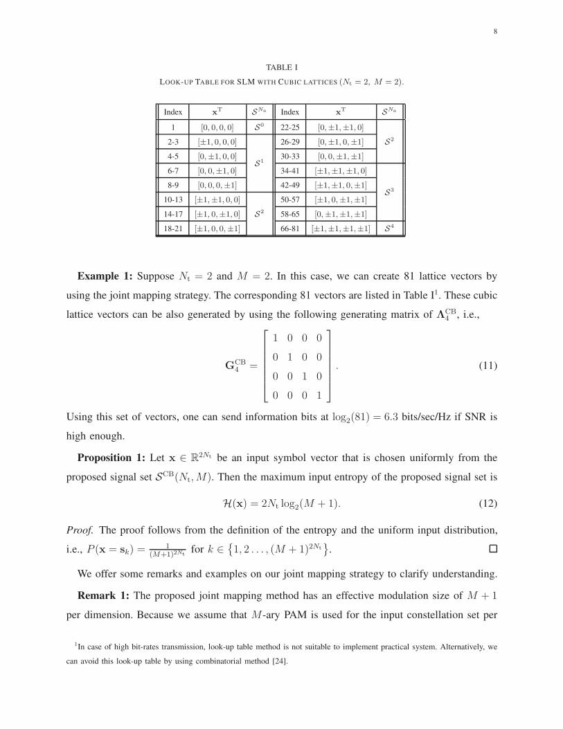
TABLE I

LOOK-UP TABLE FOR SLM WITH CUBIC LATTICES (Nt = 2, M = 2).

Index xT SNa Index x

T SNa

1 [0, 0, 0, 0] S0 22-25 [0,±1,±1, 0]

S22-3 [±1, 0, 0, 0]

S1

26-29 [0,±1, 0,±1]

4-5 [0,±1, 0, 0] 30-33 [0, 0,±1,±1]

6-7 [0, 0,±1, 0] 34-41 [±1,±1,±1, 0]

S38-9 [0, 0, 0,±1] 42-49 [±1,±1, 0,±1]

10-13 [±1,±1, 0, 0]

S2

50-57 [±1, 0,±1,±1]

14-17 [±1, 0,±1, 0] 58-65 [0,±1,±1,±1]

18-21 [±1, 0, 0,±1] 66-81 [±1,±1,±1,±1] S4

Example 1: Suppose Nt = 2 and M = 2. In this case, we can create 81 lattice vectors by

using the joint mapping strategy. The corresponding 81 vectors are listed in Table I1. These cubic

lattice vectors can be also generated by using the following generating matrix of ΛCB4 , i.e.,

GCB4 =

1 0 0 0

0 1 0 0

0 0 1 0

0 0 0 1

. (11)

Using this set of vectors, one can send information bits at log2(81) = 6.3 bits/sec/Hz if SNR is

high enough.

Proposition 1: Let x ∈ R2Nt be an input symbol vector that is chosen uniformly from the

proposed signal set SCB(Nt,M). Then the maximum input entropy of the proposed signal set is

H(x) = 2Nt log2(M + 1). (12)

Proof. The proof follows from the definition of the entropy and the uniform input distribution,

i.e., P (x = sk) =1

(M+1)2Ntfor k ∈

{1, 2 . . . , (M + 1)2Nt

}.

We offer some remarks and examples on our joint mapping strategy to clarify understanding.

Remark 1: The proposed joint mapping method has an effective modulation size of M + 1

per dimension. Because we assume that M-ary PAM is used for the input constellation set per

1In case of high bit-rates transmission, look-up table method is not suitable to implement practical system. Alternatively, we

can avoid this look-up table by using combinatorial method [24].

9

dimension, the modulation size of M is trivial. However, because we use spatial modulation, we

can add one hidden constellation point of ‘0‘ as an input vector by physically deactivating the

input per dimension; this process provides the effective modulation size of M+1. This increment

provides a considerable gain in the input entropy. For example, suppose a spatial multiplexing

transmission method with uniform M-ary PAM input signaling. The maximum input entropy of

this method is 2Nt log2(M). Therefore, one can achieve the gain of

2Nt log2(M + 1)− 2Nt log2(M) = 2Nt log2

(

1 +1

M

)

.

This entropy gain implies that one can send 2Nt log2(1 + 1

M

)more information bits per trans-

mission using the proposed method when SNR is high enough. The gain increases linearly with

Nt and is therefore unbounded.

Remark 2: The proposed joint mapping technique generalizes the existing SM methods in

[1], [6], [7], [9], [11], [14] and spatial multiplexing method. For example, supposing that Nt = 2

and M = 2, the signal sets generated by the conventional SM and QSM method in [1], [11] are

contained in S2, which is a subset of SCB(2, 2). Similarly, the signal set of the conventional spatial

multiplexing method is {1 + j, 1 − j,−1 + j,−1 − j}2, which is same with S4 of SCB(2, 2).

Remark 3: When the effective modulation size M + 1 is a prime number, the proposed

constellation set SCB(Nt,M) generated by the joint spatial mapping can also be constructed by

a nested lattice modulation method. Letting ǫ = 1√Es

, we consider two nested 2Nt-dimensional

cubic lattices with the generating matrices Gc = ǫI2Nt×2Ntand Gs = ǫ(M + 1)I2Nt×2Nt

respectively:,

Λc ={x ∈ R

2Nt : x = c⊤Gc

}and

Λs ={x ∈ R

2Nt : x = c⊤Gs

}, (13)

where c ∈ Z2Nt and Λc ⊂ Λs. Using these nested lattices, the same constellation set is generated

by

SCB(Nt,M) = Λc ∩ V0(Λs), (14)

where V0(Λs) is the Voronoi region associated with 0 ∈ Λs, i.e., the volume[

− ǫ(M+1)2

, ǫ(M+1)2

)2Nt

.

Therefore, the joint spatial mapping method can be interpreted as the nested lattice modulation

using the corresponding cubic generating matrices.

10

B. SLM with Low-Dimensional Dense Lattices

The cubic lattice ΛCB used for the previous SLM is a baseline lattice, because by the definition

it offers no nominal coding gain, i.e., γc(ΛCB

)= 1. Therefore, a natural extension is to use a

dense lattice Λ to construct a set of multi-dimensional lattice vectors that yield a higher nominal

coding gain than ΛCB in a given number of dimensions, i.e., γc (Λ) > γc(ΛCB

).

Finding the densest lattice packing in an arbitrary number of dimensions is a difficult math-

ematical problem. The lattices that have the largest nominal coding gain are well characterized

up to 24 dimensions [18], [19], [26]. The Barnes-Wall lattice is a good one due to its simplicity

of lattice construction and its tractability to analyze. It also provides high nominal coding gains

in a low-dimensional signal space.

The following lemma provides a method to construct the Barnes-Wall lattice in R2m+1

[20];

this lattice is used in the proposed SLM.

Lemma 1 (Barnes-Wall Lattice Construction [20]). Let M1 denote the generating matrix of a

balanced Barnes-Wall lattice in R2:

M1 =

√2 0

1 1

. (15)

The generating matrix of ΛBW2m+1 lattice in R2m+1

is obtained from Mm+1, which is the m + 1

times Kronecker products of M1, i.e.,

Mm+1 = M1 ⊗M1 ⊗ · · · ⊗M1︸ ︷︷ ︸

m+1

. (16)

By rescaling the irrational elements in Mm+1, the generating matrix of ΛBW2m+1 is obtained as

GBW2m+1(i, j) =

Mm+1(i, j), if Mm+1(i, j) is rational,

1√2Mm+1(i, j), if Mm+1(i, j) is irrational.

(17)

The following lemma shows some coding theoretic properties of Barnes-Wall lattices.

Lemma 2 (Coding Properties of Barnes-Wall Lattices [18], [19]). For all integer m ≥ 0, a 2m+1-

dimensional Barnes-Wall lattice ΛBW2m+1 exists that has the minimum squared Euclidean distance

d2min

(ΛBW

2m+1

)= 2m and the normalized volume V

(ΛBW

2m+1

) 1

2m = 2m2 ; therefore its nominal

coding gain is γc(ΛBW

2m+1

)= 2

m2 . In addition, the kissing number of ΛBW

2m+1 is Kmin

(ΛBW

2m+1

)=

∏m+1i=1 (2i + 2).

11

Algorithm 1 Signal Set Design Method for SLM using Dense Lattices.

Input: Generating matrix G ∈ Z2Nt×2Nt , Maximum power constraint Pmax.

Output: Signal set for SLM SBW(Nt, Pmax) ⊂ Z2Nt .

1: Initialization P = 0.

2: for P ∈ [0, 1, 2, · · · , Pmax] do

3: Define 2Nt dimensional integer row vector s = [s1, s2, . . . , s2Nt]. Then, exhaustively search s satisfying the

power condition P .

SP := {s | ‖s‖22= P, s ∈ Z2Nt , |si| ≥ |sj | , ∀ i ≥ j}.

4: Let SP denote the symmetric group, or group of permutations, on SP .

SP := {Sym{[s1, s2, . . . , s2Nt]}, ∀s ∈ SP }.

5: Check whether s is in lattice Λ.

SP := {s | s ∈ SP , sG−1 ∈ Z2Nt}..6: end for

Merge all SP sets into SBW.

7: SBW(Nt, Pmax) = ∪Pmax

P=0SP .

By exploiting the Barnes-Wall lattice ΛBW2m+1 that is constructed by GBW

m+1 in (17), we propose

Algorithm 1, which creates a signal set for SLM using dense lattices. The algorithm finds a

signal set SBW such that each lattice vector is created by generating matrix G ∈ Z2Nt×2Nt and

satisfies the maximum power constraint Pmax. The first step is to exhaustively search all possible

integer vectors that satisfy the given power P . For a vector satisfying the power constraint, the

symmetric group is selected as a candidate. For example, with ΛBW4 lattice at power condition

P = 2, [±1,±1,0,0], [±1,0,±1,0], [ ±1,0,0,±1 ], [0,±1,±1,0], [0,±1,0,±1], [0,0,±1,±1] will be

the possible candidates for constellation vectors. After collecting the candidates, we check the

condition whether they consist of an integer linear combination of the basis {g1, . . . , g2Nt}. Then,

vectors that satisfy this condition are included in our SLM signal set. Algorithm 1 iterates this

procedure by increasing P until the power condition P reaches the maximum power constraint

Pmax.

Example 2: Suppose a four-dimensional Barnes-Wall lattice, ΛBW4 , which is equivalent to the

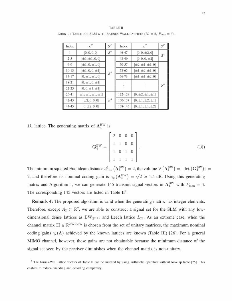
12

TABLE II

LOOK-UP TABLE FOR SLM WITH BARNES-WALL LATTICES (Nt = 2, Pmax = 6).

Index xT SP Index x

T SP

1 [0, 0, 0, 0] S0 46-47 [0, 0,±2, 0]S4

2-5 [±1,±1, 0, 0]

S2

48-49 [0, 0, 0,±2]

6-9 [±1, 0,±1, 0] 50-57 [±2,±1,±1, 0]

S6

10-13 [±1, 0, 0,±1] 58-65 [±1,±2,±1, 0]

14-17 [0,±1,±1, 0] 66-73 [±1,±1,±2, 0]

18-21 [0,±1, 0,±1] ...

..

.22-25 [0, 0,±1,±1]

26-41 [±1,±1,±1,±1]

S4

122-129 [0,±2,±1,±1]

42-43 [±2, 0, 0, 0] 130-137 [0,±1,±2,±1]

44-45 [0,±2, 0, 0] 138-145 [0,±1,±1,±2]

D4 lattice. The generating matrix of ΛBW4 is

GBW4 =

2 0 0 0

1 1 0 0

1 0 1 0

1 1 1 1

. (18)

The minimum squared Euclidean distance d2min

(ΛBW

4

)= 2, the volume V

(ΛBW

4

)= | det

(GBW

4

)| =

2, and therefore its nominal coding gain is γc(ΛBW

4

)=

√2 ≃ 1.5 dB. Using this generating

matrix and Algorithm 1, we can generate 145 transmit signal vectors in ΛBW4 with Pmax = 6.

The corresponding 145 vectors are listed in Table II2.

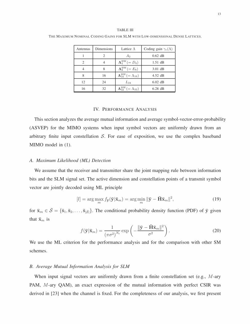
Remark 4: The proposed algorithm is valid when the generating matrix has integer elements.

Therefore, except A2 ⊂ R2, we are able to construct a signal set for the SLM with any low-

dimensional dense lattices as BW2m+1 and Leech lattice L24. As an extreme case, when the

channel matrix H ∈ R2Nr×2Nt is chosen from the set of unitary matrices, the maximum nominal

coding gains γc(Λ) achieved by the known lattices are known (Table III) [26]. For a general

MIMO channel, however, these gains are not obtainable because the minimum distance of the

signal set seen by the receiver diminishes when the channel matrix is non-unitary.

2 The barnes-Wall lattice vectors of Table II can be indexed by using arithmetic operators without look-up table [25]. This

enables to reduce encoding and decoding complexity.

13

TABLE III

THE MAXIMUM NOMINAL CODING GAINS FOR SLM WITH LOW-DIMENSIONAL DENSE LATTICES.

Antennas Dimensions Lattice Λ Coding gain γc(Λ)

1 2 A2 0.62 dB

2 4 ΛBW4 (= D4) 1.51 dB

4 8 ΛBW8 (= E8) 3.01 dB

8 16 ΛBW16 (= Λ16) 4.52 dB

12 24 L24 6.02 dB

16 32 ΛBW32 (= Λ32) 6.28 dB

IV. PERFORMANCE ANALYSIS

This section analyzes the average mutual information and average symbol-vector-error-probability

(ASVEP) for the MIMO systems when input symbol vectors are uniformly drawn from an

arbitrary finite input constellation S. For ease of exposition, we use the complex baseband

MIMO model in (1).

A. Maximum Likelihood (ML) Detection

We assume that the receiver and transmitter share the joint mapping rule between information

bits and the SLM signal set. The active dimension and constellation points of a transmit symbol

vector are jointly decoded using ML principle

[l] = argmaxm

fy(y|xm) = argminm

‖y − Hxm‖2, (19)

for xm ∈ S = {s1, s2, . . . , s|S|}. The conditional probability density function (PDF) of y given

that xm is

f(y|xm) =1

(πσ2)Nrexp

(

−‖y − Hxm‖2σ2

)

. (20)

We use the ML criterion for the performance analysis and for the comparison with other SM

schemes.

B. Average Mutual Information Analysis for SLM

When input signal vectors are uniformly drawn from a finite constellation set (e.g., M-ary

PAM, M-ary QAM), an exact expression of the mutual information with perfect CSIR was

derived in [23] when the channel is fixed. For the completeness of our analysis, we first present

14

the exact expression of the mutual information. Then, to improve intuition, we also provide a

tight approximation expression for the average mutual information.

1) Exact Expression: For a MIMO channel, the mutual information between the discrete input

vector x and the continuous channel output vector y is

I(x; y|H) = H(y|H)−H(y|x, H)

= H(y|H)−H(v)

= H(y|H)−Nr log2(πeσ2). (21)

Because the received signal vector y follows a Gaussian distribution for given H and x, the

PDF of y is

f(y|H) =1

|S|∑

xi∈S

1

(πσ2)Nrexp

(

−‖y − Hxi‖2σ2

)

. (22)

Using f(y|xi, H) and f(y|H), the mutual information for given H is

I(x; y|H) =∑

xi∈S

1

|S|

∫

y

f(y|x = xi, H) log2f(y|x = xi, H)

f(y|H)dy. (23)

Using equations (21)-(23), the mutual information for SLM is obtained as

I(x; y|H) = log |S|

− 1

|S|∑

xi∈SEv

log2∑

xj∈Sexp

(

−‖H(xi − xj)+v‖2−‖v‖2σ2

)

. (24)

2) Approximation of Average Mutual Information: The derived mutual information expression

in (24) is not tractable because it involves the multi-dimensional integral with respect to v and

it does not capture the randomness in channels. We derive a closed form tight approximation of

the average mutual information by exploiting the lower bound of (24). The following proposition

closely approximates the average mutual information.

Proposition 3: The average mutual information, EH

[I(x; y|H

)]for SLM, can be approxi-

mated as

EH

[I(x; y|H

)]

≈ 2 log2 |S| − log2∑

xi∈S

∑

xj∈S

(

1 +‖xi − xj‖2

2σ2

)−Nr

. (25)

15

Proof. Applying Jensen’s inequality yields a lower bound of H(y|H) as in [23],

H(y|H) ≥ − log2 Ey

[f(y|H)

]=

− log2

∫

y

(

1

|S|∑

xi∈S

1

(πσ2)Nrexp

(

−‖y − Hxi‖2σ2

))2

dy. (26)

By changing the order of summation and integration in (26), H(y|H) is lower-bounded by

H(y|H) ≥ 2 log2 |S|(πσ2)Nr

− log2∑

xi∈S

∑

xj∈S

∫

y

e−‖y−Hxi‖

2

σ2 e−‖y−Hxj‖

2

σ2 dy. (27)

The integration in (27) can be calculated as∫

y

e−‖y−Hxi‖

2

σ2 e−‖y−Hxj‖

2

σ2 dy = e−‖Hxi‖

2+‖Hxj‖

2

σ2 ×∫

y

exp

(

−2‖y‖2 − 2Re{yH(Hxi + Hxj)

}

σ2

)

dy

︸ ︷︷ ︸

Θ

. (28)

Because the elements of y = [y1, y2, . . . , yNr]⊤ are mutually independent, the multi-dimensional

integrations in (28) are computed using element-wise integrations as

Θ =Nr∏

k=1

∫

yk

exp

(

−2‖yk‖2 − 2Re

{y∗k{H(xi + xj)

}

k

}

σ2

)

dyk. (29)

The integration in (29) is conducted separately for real and imaginary parts to yield

∫

yk,Re

exp

(

−2y2k,Re − 2yk,Re

{H(xi + xj)

}

k,Re

σ2

)

dyk,Re

×∫

yk,Im

exp

(

−2y2k,Im − 2yk,Im

{H(xi + xj)

}

k,Im

σ2

)

dyk,Im. (30)

The integrals in (30) are computed using the following identity

∫ ∞

−∞exp

(

−2y2 − 2xy

σ2

)

dy =

√

πσ2

2exp

(x2

2σ2

)

. (31)

Thus, Θ = ΘRe ×ΘIm, where ΘRe and ΘIm are given by

ΘRe =

Nr∏

k=1

√

πσ2

2exp

{H(xi + xj)

}2

k,Re

σ2

,

ΘIm =

Nr∏

k=1

√

πσ2

2exp

{H(xi + xj)

}2

k,Im

σ2

. (32)

16

Using the results in (32), we obtain the simple

Θ =Nr∏

k=1

(πσ2

2

)

exp

(∥∥{H(xi + xj)

}

k

∥∥2

2σ2

)

=

(πσ2

2

)Nr

exp

(‖H(xi + xj)‖22σ2

)

. (33)

Using the above equations (27)-(33), the lower bound of H(y|H) is

H(y|H) ≥ 2 log2 |S|+ log2(πσ2)Nr +Nr log2 2

− log2∑

xi∈S

∑

xj∈Sexp

(

−‖H(xi − xj)‖22σ2

)

. (34)

Plugging (34) into (21), a lower bound of I(x; y|H) is obtained as

ILow(x; y|H) = 2 log2 |S|+Nr log22

e

− log2∑

xi∈S

∑

xj∈Sexp

(

−‖H(xi − xj)‖22σ2

)

= 2 log2 |S|+Nr log22

e

− log2

|S|+

∑

xi∈S

∑

xj∈S/{xi}exp

(

−‖H(xi − xj)‖22σ2

)

. (35)

From (35), by taking the limits to the two extreme SNR regimes, we obtain the limit values:

limSNR→0

ILow(x; y|H) = Nr log22

e,

limSNR→∞

ILow(x; y|H) = Nr log22

e+ log2 |S|. (36)

Intuitively, the mutual information should approach zero when SNR is very low, but should

approach log2 |S| when SNR is very high. Using these facts and the two extreme values in (36),

we define the offset for the approximation as,

△I(x;y|H) = ILow(x; y|H)− I(x; y|H) = Nr log2e

2. (37)

Subtracting this offset yields a tight approximation of I(x; y|H):

I(x; y|H) = 2 log2 |S| − log2∑

xi∈S

∑

xj∈Sexp

(

−‖H(xi − xj)‖22σ2

)

= − log21

|S|2∑

xi∈S

∑

xj∈Sexp

(

−‖H(xi − xj)‖22σ2

)

. (38)

17

In (38), the elements of H follow the complex Gaussian distribution. Therefore, for given

symbol vectors xi, xj , κ =‖H(xi−xj)‖2

2σ2 follows the Gamma distribution with PDF fκ(w) ∼Γ(

Nr,‖xi−xj‖2

2σ2

)

. The exception of the mutual information is approximated by applying Jensen’s

inequality to I as

EH

[I(x; y|H

)]≈ EH

[

I(x; y|H

)]

≥ − log21

|S|2∑

xi∈S

∑

xj∈SEH

[

exp

(

−‖H(xi − xj)‖22σ2

)]

. (39)

The lower bound is due to the concavity of the log function. In addition, the expectation in

(39) is simply calculated using the moment generating function (MGF) of the Gamma random

variable κ, i.e., E [e−κ] =(

1 +‖xi−xj‖2

2σ2

)−Nr

. As a result, the approximate expression of the

average mutual information is

EH

[I(x; y|H

)]≈ − log2

1

|S|2∑

xi∈S

∑

xj∈S

(

1 +‖xi − xj‖2

2σ2

)−Nr

= 2 log2 |S| − log2∑

xi∈S

∑

xj∈S

(

1 +‖xi − xj‖2

2σ2

)−Nr

, (40)

which completes the proof.

Because the proposed SLM uses a set of lattice points with symmetric minimum distance,

i.e., ‖xi − xj‖2 ≥ d2min(Λ), (xi 6= xj), we can further simplify the average mutual information

in the following corollary:

Corollary 1: A lower bound of EH

[

I(x; y|H

)]

for SLM using lattice Λ is

EH

[

I(x; y|H

)]

≥ log2 |S| − log2

(

1 + (|S| − 1)

(

1 +d2min(Λ)

2σ2

)−Nr

)

. (41)

The result in Corollary 1 clearly shows that a higher average mutual information is achievable

when dense lattices (or equivalently a large d2min(Λ)) are used and the number of receive antennas

increases.

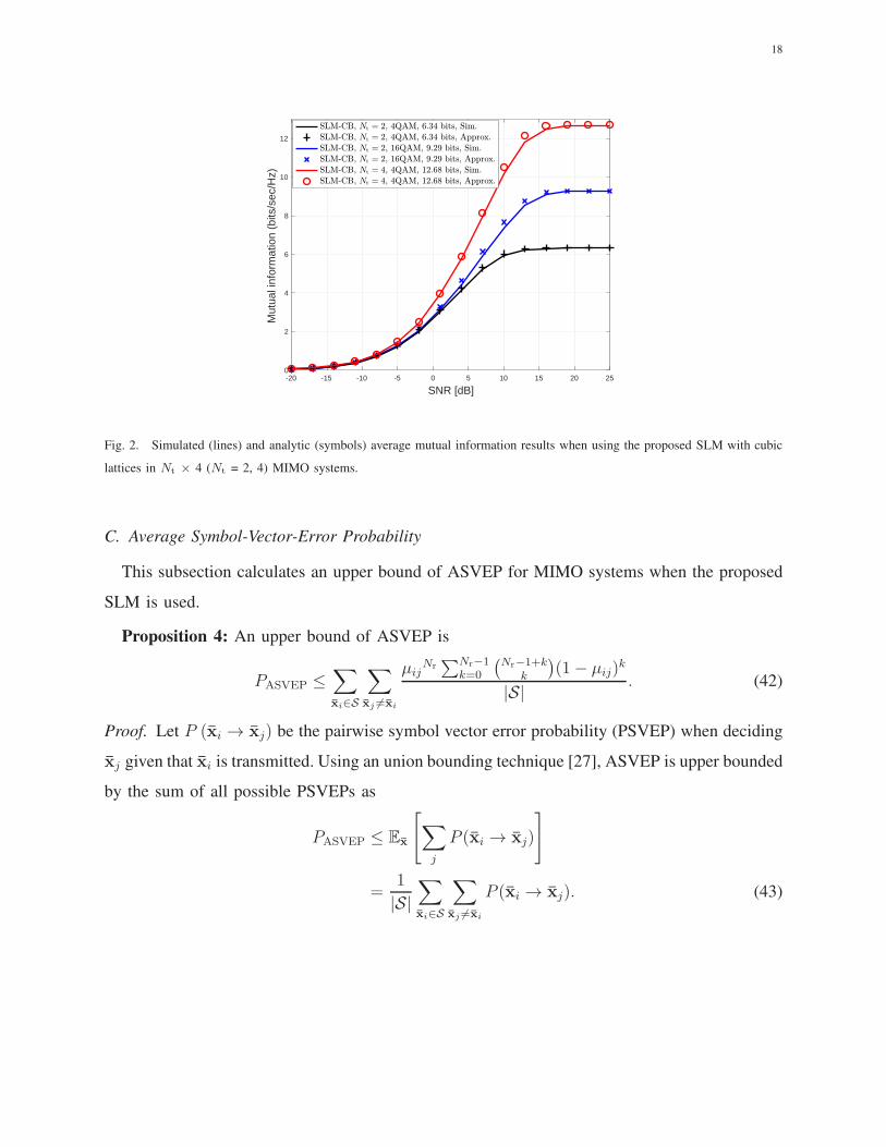
Fig. 2 shows that the proposed approximation of the average mutual information derived in (40)

agrees well with simulations at all SNR region for MIMO systems with antenna configurations

(Nt, Nr,M) = (2, 4, 2), (2, 4, 4), and (4, 4, 2), and various modulation sizes.

18

-20 -15 -10 -5 0 5 10 15 20 25

SNR [dB]

0

2

4

6

8

10

12

Mut

ual i

nfor

mat

ion

(bits

/sec

/Hz)

Fig. 2. Simulated (lines) and analytic (symbols) average mutual information results when using the proposed SLM with cubic

lattices in Nt × 4 (Nt = 2, 4) MIMO systems.

C. Average Symbol-Vector-Error Probability

This subsection calculates an upper bound of ASVEP for MIMO systems when the proposed

SLM is used.

Proposition 4: An upper bound of ASVEP is

PASVEP ≤∑

xi∈S

∑

xj 6=xi

µijNr∑Nr−1

k=0

(Nr−1+k

k

)(1− µij)

k

|S| . (42)

Proof. Let P (xi → xj) be the pairwise symbol vector error probability (PSVEP) when deciding

xj given that xi is transmitted. Using an union bounding technique [27], ASVEP is upper bounded

by the sum of all possible PSVEPs as

PASVEP ≤ Ex

[∑

j

P (xi → xj)

]

=1

|S|∑

xi∈S

∑

xj 6=xi

P (xi → xj). (43)

19

By using the ML detection principle in (19), PSVEP conditioned on H is given by

P (xi → xj |H) = P(

‖v + H(xi − xj)‖2 < ‖v‖2∣∣∣ H)

= P

(

Re{vHH(xi − xj)

}< −1

2‖H(xi − xj)‖2

∣∣∣ H

)

= Q(√

κ), (44)

where Q(x) =∫∞x

1√2πe−

t2

2 dt denotes the tail probability of a standard Gaussian distribution.

Thus, the PSVEP is obtained by computing the integral, i.e.,

P (xi → xj) = EH

[

P (xi → xj

∣∣∣H)

]

=

∫ ∞

w=0

Q(√

w)fκ(w)dw

= µijNr

Nr−1∑

k=0

(Nr − 1 + k

k

)

(1− µij)k, (45)

where µij =12

(

1−√

‖xi−xj‖24σ2+‖xi−xj‖2

)

and the third equality follows from the closed form expres-

sion given in [28]. Substituting (45) into (43) yields

PASVEP ≤∑

xi∈S

∑

xj 6=xi

µijNr∑Nr−1

k=0

(Nr−1+k

k

)(1− µij)

k

|S| , (46)

which completes the proof.

We can further simplify ASVEP in Proposition 4 by using the well known upper bound of

the Gaussian Q-function. Using following inequality Q(x) ≤ 12exp

(

−x2

2

)

, the SVPEP in (44)

is upper bounded by

P (xi → xj |H) = Q(√

κ)≤ 1

2exp

(

−κ

2

)

. (47)

By marginalizing with respect to κ

P (xi → xj) ≤1

2Eκ

[

exp(

−κ

2

)]

. (48)

Using the MGF of the Gamma distribution yields

P (xi → xj) ≤1

2

(

1 +‖xi − xj‖2

4σ2

)−Nr

. (49)

Consequently, from (43), we obtain the upper bound as

PASVEP ≤ 1

2|S|∑

xi∈S

∑

xj 6=xi

(

1 +‖xi − xj‖2

4σ2

)−Nr

, (50)

20

which is a similar form of (40).

From the fact that ‖xi − xj‖2 ≥ d2min(Λ)(xi 6= xj), we further simplify (50) in the following

corollary.

Corollary 2: A lower bound of ASVEP for SLM using lattice Λ is

PASVEP ≤ 1

2|S|∑

xi∈S

∑

xj 6=xi

(

1 +d2min(Λ)

4σ2

)−Nr

=(|S| − 1)

2

(

1 +d2min(Λ)

4σ2

)−Nr

. (51)

Similar to Corollary 1, the result in Corollary 2 shows that ASVEP decreases as the minimum

distance of the lattice d2min(Λ) increases or the number of receive antennas Nr increases.

V. LATTICE SPHERE DECODING

In this section, we present a low complexity detection method for SLM, referred to as

lattice sphere decoding (LSD). One drawback of the SLM introduced in Section III is that

the ML detection complexity increases exponentially with the number of transmit antennas or

the modulation size, i.e., O((M + 1)2Nt

). Therefore, for massive MIMO systems with a large

number of transmit antennas, SLM is not appropriate due to the forbidding detection complexity.

The proposed LSD overcomes this drawback by reducing the effective search space to the closest

lattice vectors from an initially estimated lattice vector.

A. Lattice Sphere Decoding

This subsection explains the key idea and the algorithm of lattice sphere decoding (LSD). The

core idea of LSD is to search only the closest lattice vectors from an initially estimated lattice

vector.

1) Initial estimate: The first step of LSD is to find an initial estimate x by using linear

detection methods such as a minimum mean-square error (MMSE) detection method, namely,

x =

(

H⊤H+σ2

Es/Nt

I

)−1

H⊤y. (52)

2) Vector quantization: The estimated x is quantized to the closest lattice vector by using

the vector quantization function3 Q : R2Nt → ΛBW in [29], i.e.,

x = Q(x). (53)

3For more details on the lattice vector quantization in [29], see Appendix A.

21

Since the transmitted signal is a lattice vector that satisfies the maximum power constraint Pmax

by the construction of SLM, we need to rescale the initial estimate x if ‖Q(x)‖2 > Pmax, i.e.,

x = Q

(x

‖x‖√

Pmax

)

. (54)

3) Reduced lattice set construction inside a sphere: We construct a subset XBW ⊂ ΛBW

whose elements lie in the sphere centered at the quantization output vector x with radius of d.

In particular, we set the radius to the smallest Euclidean norm, i.e., d = d2min(ΛBW). This sphere

radius guarantees that the cardinality of X is equal to the kissing number of a lattice plus one,

i.e, |XBW| = Kmin(ΛBW) + 1.

Using the fact that a lattice is closed under addition, we find the elements of the subset XBW

in a systematic manner. Let define a set Dmin that has elements with the smallest Euclidean

norm d2min(Λ), i.e., the set with the closest lattice vectors from origin. By the lattice property,

the cardinality of Dmin is equal to the kissing number of a lattice, i.e, |Dmin| = Kmin(Λ). Using

Dmin, it is possible to find the elements of XBW by adding the initial estimate lattice point x to

the elements in Dmin, namely,

XBW = {x|x = x+ d,d ∈ Dmin ∪ {0}}. (55)

Under the maximum power constraint Pmax, the set XBW is further reduced to a set XBW by

only merging the vectors which satisfy this power constraint.

XBW = {x|x ∈ XBW, ||x||2 ≤ Pmax}. (56)

4) Decoding over the reduced set: Using the reduced lattice set in the sphere, XBW, the

receiver performs ML detection over the reduced set, i.e.,

s = arg minx∈XBW

||y−Hx||2. (57)

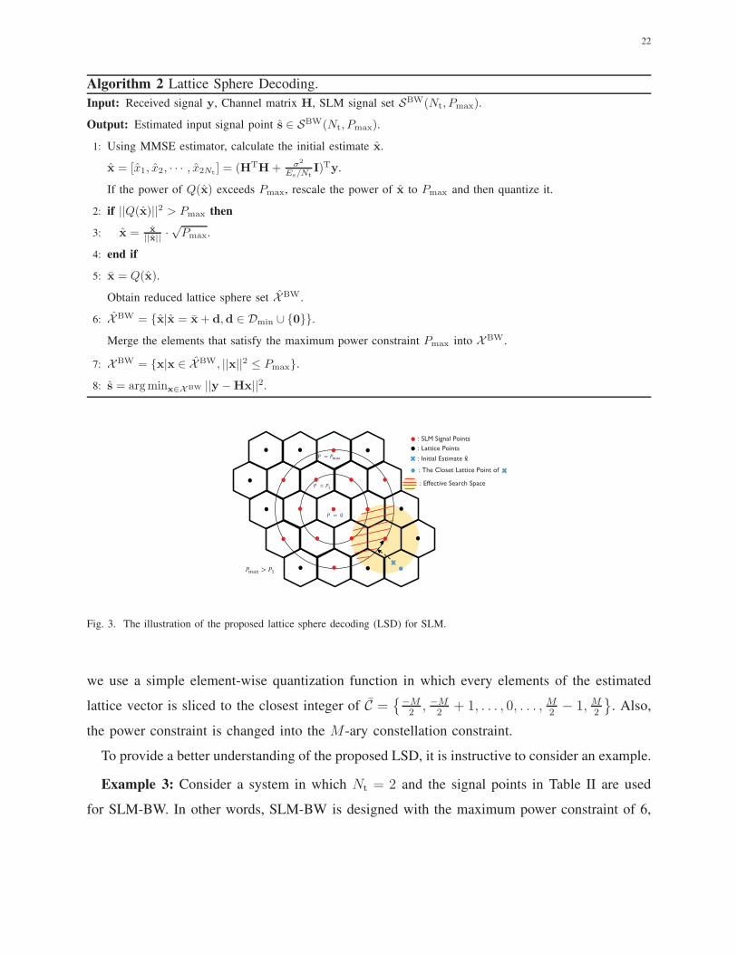
As seen in Fig. 3, the blue x-mark represents the initial estimate x. This blue x-mark is

quantized to the lattice vector (the blue circle). Because the power of the blue circle exceeds Pmax,

the blue x-mark are rescaled and re-quantized. Then, we obtain the lattice set inside the sphere

(the red stripes region), which includes the quantized lattice vector. Finally, we calculate ML

metrics over the reduced lattice set XBW. The proposed algorithm is summarized in Algorithm

2.

Throughout this section, we mainly focus on LSD with Barnes-Wall lattices. With a similar

manner, we are able to extend the LSD algorithm for cubic lattices. In the case of cubic lattices,

22

Algorithm 2 Lattice Sphere Decoding.

Input: Received signal y, Channel matrix H, SLM signal set SBW(Nt, Pmax).

Output: Estimated input signal point s ∈ SBW(Nt, Pmax).

1: Using MMSE estimator, calculate the initial estimate x.

x = [x1, x2, · · · , x2Nt] = (HTH+ σ2

Es/Nt

I)Ty.

If the power of Q(x) exceeds Pmax, rescale the power of x to Pmax and then quantize it.

2: if ||Q(x)||2 > Pmax then

3: x = x

||x|| ·√Pmax.

4: end if

5: x = Q(x).

Obtain reduced lattice sphere set XBW.

6: XBW = {x|x = x+ d,d ∈ Dmin ∪ {0}}.

Merge the elements that satisfy the maximum power constraint Pmax into XBW.

7: XBW = {x|x ∈ XBW, ||x||2 ≤ Pmax}.8: s = argminx∈XBW ||y −Hx||2.

: SLM Signal Points

: Lattice Points

: Initial Estimate

: The Closet Lattice Point of

: Effective Search Space

= 0

=

=

>

Fig. 3. The illustration of the proposed lattice sphere decoding (LSD) for SLM.

we use a simple element-wise quantization function in which every elements of the estimated

lattice vector is sliced to the closest integer of C ={−M

2, −M

2+ 1, . . . , 0, . . . , M

2− 1, M

2

}. Also,

the power constraint is changed into the M-ary constellation constraint.

To provide a better understanding of the proposed LSD, it is instructive to consider an example.

Example 3: Consider a system in which Nt = 2 and the signal points in Table II are used

for SLM-BW. In other words, SLM-BW is designed with the maximum power constraint of 6,

23

i.e., Pmax = 6. Following by Algorithm 2, we firstly obtain an initial estimate x. For example,

x = [+1.32, − 2.51, − 0.41, + 2.70]T . (58)

Then, x is quantized to the closest lattice vector Q(x)4.

Q(x) = [+1, − 2, 0, + 3]T . (59)

The power of Q(x) equals 14. Therefore, we rescale the power of x to Pmax.

x

‖x‖√

Pmax = [+0.82, − 1.57, − 0.25, + 1.68]T .

x = Q

(x

‖x‖√

Pmax

)

= [+1, − 1, 0, + 2]T . (60)

After obtaining the quantized output x, the lattice sphere set XBW is generated. XBW of SLM-

BW is obtained by adding x to Dmin(= S2 in Table II) and removing the elements that violate

the power constraint as follows:

XBW =

+1

−1

0

+2

,

0

0

0

+2

,

0

−1

−1

+2

, · · · ,

+1

−2

0

+1

,

+1

−1

−1

+1

. (61)

Then, the receiver calculates the ML metrics over the twelve symbol vectors in XBW and decides

a symbol vector that has the minimum value of ‖y−Hx‖2. Similarly, the receiver performs the

same procedure for SLM-CB.

B. Detection Complexity Analysis

In this subsection, the detection complexities of the proposed LSD and ML detectors for SLM

are analyzed. In addition, these are compared to the complexities of detectors for the existing

spatial modulation and the spatial multiplexing method. Each real addition, multiplication, and

rounding operation are counted as one floating operation (flop).

1) MLD: Let Na be the the number of activated dimensions in an 2Nt-dimensional real space.

Therefore, Na of SM equals 2, Na of spatial multiplexing equals 2Nt, and Na of SLM has values

between 0 and 2Nt. The complexity of ML detector in (19) can be computed as follows:

• The operator Hx requires NrNa real multiplications and Nr(Na − 1) real additions.

4In Appendix A, we provide the quantization procedures of x as an example.

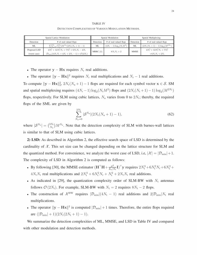
24

TABLE IV

DETECTION COMPLEXITIES OF VARIOUS MODULATION METHODS.

Spatial Lattice Modulation Spatial Modulation Spatial Multiplexing

Detection # of real-valued flops Detection # of real-valued flops Detection # of real-valued flops

ML∑2Nt

Na=0

(

2Nt

Na

)

MNa(2Nr(Na + 1)− 1) ML (4Nr − 1) log2(NtM2) ML (2Nr(Nt + 1) − 1) log2(M

2Nt )

Proposed LSD

(worst case)

4N3t + 12N2

t Nr + 7N2t + 6NtNr − 4Nt

|Dmin|(4NtNr + 4Nt + 2Nr − 1) +O(2Nt)MRRC [1] 8NtNr + 2 MMSE

4N3t + 12N2

t Nr + 7N2t

+6NtNr + 2Nt

• The operator y −Hx requires Nr real additions.

• The operator ‖y −Hx‖2 requires Nr real multiplications and Nr − 1 real additions.

To compute ‖y −Hx‖22, 2Nr(Na+1)− 1 flops are required for each symbol vector x ∈ S. SM

and spatial multiplexing requires (4Nr−1) log2(NtM2) flops and (2Nr(Nt+1)−1) log2(M

2Nt)

flops, respectively. For SLM using cubic lattices, Na varies from 0 to 2Nt; thereby, the required

flops of the SML are given by

2Nt∑

Na=0

|SNa |(2Nr(Na + 1)− 1), (62)

where |SNa | =(2Nt

Na

)MNa . Note that the detection complexity of SLM with barnes-wall lattices

is similar to that of SLM using cubic lattices.

2) LSD: As described in Algorithm 2, the effective search space of LSD is determined by the

cardinality of X . This set size can be changed depending on the lattice structure for SLM and

the quantized method. For convenience, we analyze the worst case of LSD, i.e, |X | = |Dmin|+1.

The complexity of LSD in Algorithm 2 is computed as follows:

• By following [30], the MMSE estimator (H⊤H+ σ2

Es/NtI)⊤y requires 2N3

t +6N2t Nr+6N2

t +

4NtNr real multiplications and 2N3t + 6N2

t Nr +N2t + 2NtNr real additions.

• As indicated in [29], the quantization complexity order of SLM-BW with Nt antennas

follows O (2Nt). For example, SLM-BW with Nt = 2 requires 8Nt − 2 flops.

• The construction of XBW requires |Dmin|(4Nt − 1) real additions and 2|Dmin|Nt real

multiplications.

• The operator ‖y−Hx‖2 is computed |Dmin|+1 times. Therefore, the entire flops required

are (|Dmin|+ 1)(2Nr(2Nt + 1)− 1).

We summarize the detection complexities of ML, MMSE, and LSD in Table IV and compared

with other modulation and detection methods.

25

VI. NUMERICAL RESULTS

This section provides numerical results on the average mutual information, uncoded symbol-

vector-error-rate (SVER), and coded frame-error-rate (FER) of the proposed SLM methods. These

metrics are used to show SNR gains compared to the existing SM and the spatial multiplexing

techniques. All results are obtained by using Monte Carlo simulations on independent flat-fading

channel realizations for various spectral efficiencies as a function of SNR.

A. Average Mutual Information

Fig. ?? depicts the achievable spectral efficiencies of various transmission strategies for a

MIMO system with Nt = 2, Nr = 4, and the M-PAM input constellation set per in-phase

and quadrature component (equivalently, M2-QAM). The solid-black line shows the capacity of

2× 4 MIMO channel when using Gaussian input signaling, which serves an upper bound of the

spectral efficiencies attained by the other transmission methods. In Fig. ??, the proposed SLM

method with cubic lattices (SLM-CB) uses 4-PAM per dimension, which is able to generates

54 lattice symbol vectors. In case of SLM with Barnes-Wall lattices (SLM-BW), we select 54

elements from SBW(2, 18) in ascending order of the power consumption. The proposed SLM-CB

and SLM-BW both achieve the spectral efficiency of log2(54) ≈ 9.29 bits/sec/Hz beyond 20 dB

SNR. Especially, SLM-BW achieves higher spectral efficiency than that of SLM-CB in the mid

SNR because Barnes-Wall lattices provide a higher nominal coding gain than do cubic lattices,

γ(ΛBW4 ) > γ(ΛCB

4 ). In contrast, spatial multiplexing and SM achieve the spectral efficiencies

of 8 bits/sec/Hz and 5 bits/sec/Hz respectively when SNR is high enough. Similar results are

observed when 2-ary PAM input signal is used. Thus, SLM achieves the higher spectral efficiency

than do the conventional methods.

B. Symbol Vector Error Rate

We compare the SVERs of the proposed SLM methods with that of the existing SM, GSM,

GSM-Eisenstein, ESM, and spatial multiplexing methods. For fair comparisons, each modulation

scheme is allowed to use a different modulation size M to achieve similar target spectral

efficiencies. It should be noted that the results of Fig. 5 and Fig. 6 are obtained under ML

detection and the results of Fig. 7 and Fig. 8 are obtained under ML detection and LSD.

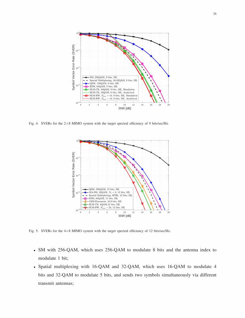
Fig. 4 shows the SVERs when the target spectral efficiency is 9 bits/sec/Hz for the 2 × 8

MIMO system. To meet this criterion, we set different modulation size for each method:

26

0 2 4 6 8 10 12 14 16 18 20

SNR [dB]

10 -4

10 -3

10 -2

10 -1

100

Sym

bol V

ecto

r E

rror

Rat

e (S

VE

R)

Fig. 4. SVERs for the 2×8 MIMO system with the target spectral efficiency of 9 bits/sec/Hz.

0 2 4 6 8 10 12 14 16 18 20

SNR [dB]

10 -4

10 -3

10 -2

10 -1

100

Sym

bol V

ecto

r E

rror

Rat

e (S

VE

R)

Fig. 5. SVERs for the 4×8 MIMO system with the target spectral efficiency of 12 bits/sec/Hz.

• SM with 256-QAM, which uses 256-QAM to modulate 8 bits and the antenna index to

modulate 1 bit;

• Spatial multiplexing with 16-QAM and 32-QAM, which uses 16-QAM to modulate 4

bits and 32-QAM to modulate 5 bits, and sends two symbols simultaneously via different

transmit antennas;

27

• ESM with 64-QAM, which uses 64-QAM as a primary signal constellation set to modulate

9 bits;

• QSM with 128-QAM, which uses 128-QAM to modulate 7 bits and the antenna indies to

modulate 2 bit;

• SLM-CB with 16-QAM, which is constructed by selecting 512 elements from SCB(2, 4) in

ascending order of the power consumption to modulate 9 bits;

• SLM-BW, which is constructed by selecting 512 elements from SBW(2, 14) in ascending

order of the power consumption to modulate 9 bits;

Fig. 4 shows that the proposed SLM-CB and SLM-BW achieve lower SVERs than all other

transmission methods at all SNR. SLM-CB provides about 1 dB SNR gain over the spatial

multiplexing at SVER = 10−3. SLM-BW provides 1 dB SNR gain over SLM-CB. This increase

occurs because the Barnes-Wall lattice has a larger nominal coding gain than does cubic lattice.

In addition, our analytic expression of SVER obtained from (46) is shown to be tight at high

SNR.

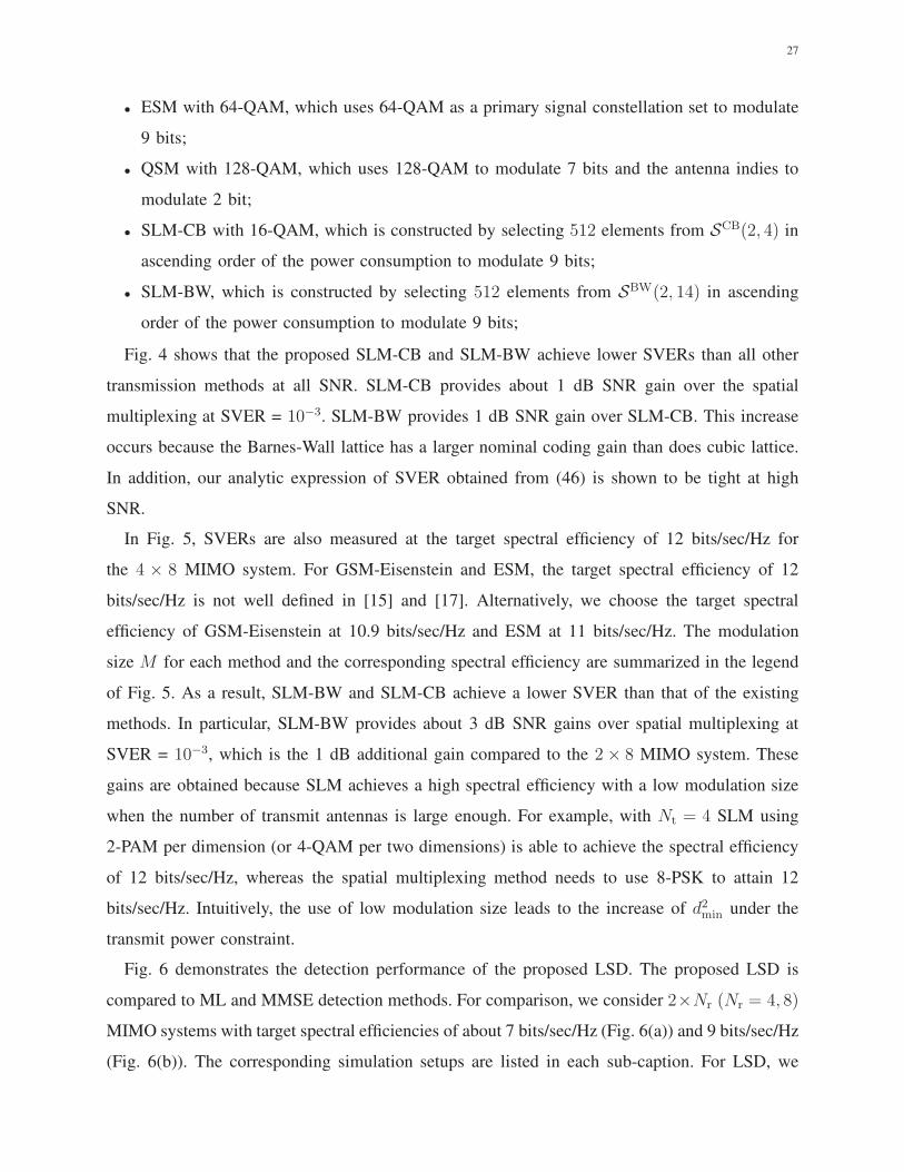
In Fig. 5, SVERs are also measured at the target spectral efficiency of 12 bits/sec/Hz for

the 4 × 8 MIMO system. For GSM-Eisenstein and ESM, the target spectral efficiency of 12

bits/sec/Hz is not well defined in [15] and [17]. Alternatively, we choose the target spectral

efficiency of GSM-Eisenstein at 10.9 bits/sec/Hz and ESM at 11 bits/sec/Hz. The modulation

size M for each method and the corresponding spectral efficiency are summarized in the legend

of Fig. 5. As a result, SLM-BW and SLM-CB achieve a lower SVER than that of the existing

methods. In particular, SLM-BW provides about 3 dB SNR gains over spatial multiplexing at

SVER = 10−3, which is the 1 dB additional gain compared to the 2× 8 MIMO system. These

gains are obtained because SLM achieves a high spectral efficiency with a low modulation size

when the number of transmit antennas is large enough. For example, with Nt = 4 SLM using

2-PAM per dimension (or 4-QAM per two dimensions) is able to achieve the spectral efficiency

of 12 bits/sec/Hz, whereas the spatial multiplexing method needs to use 8-PSK to attain 12

bits/sec/Hz. Intuitively, the use of low modulation size leads to the increase of d2min under the

transmit power constraint.

Fig. 6 demonstrates the detection performance of the proposed LSD. The proposed LSD is

compared to ML and MMSE detection methods. For comparison, we consider 2×Nr (Nr = 4, 8)

MIMO systems with target spectral efficiencies of about 7 bits/sec/Hz (Fig. 6(a)) and 9 bits/sec/Hz

(Fig. 6(b)). The corresponding simulation setups are listed in each sub-caption. For LSD, we

28

10 15 20 25 30

SNR [dB]

10-5

10-4

10-3

10-2

10-1

100

Sym

bol V

ecto

r E

rror

Rate

(S

VE

R)

Nr = 8

Nr = 4

(a)

10 15 20 25 30

SNR [dB]

10-5

10-4

10-3

10-2

10-1

100

Nr = 8

Nr = 4

(b)

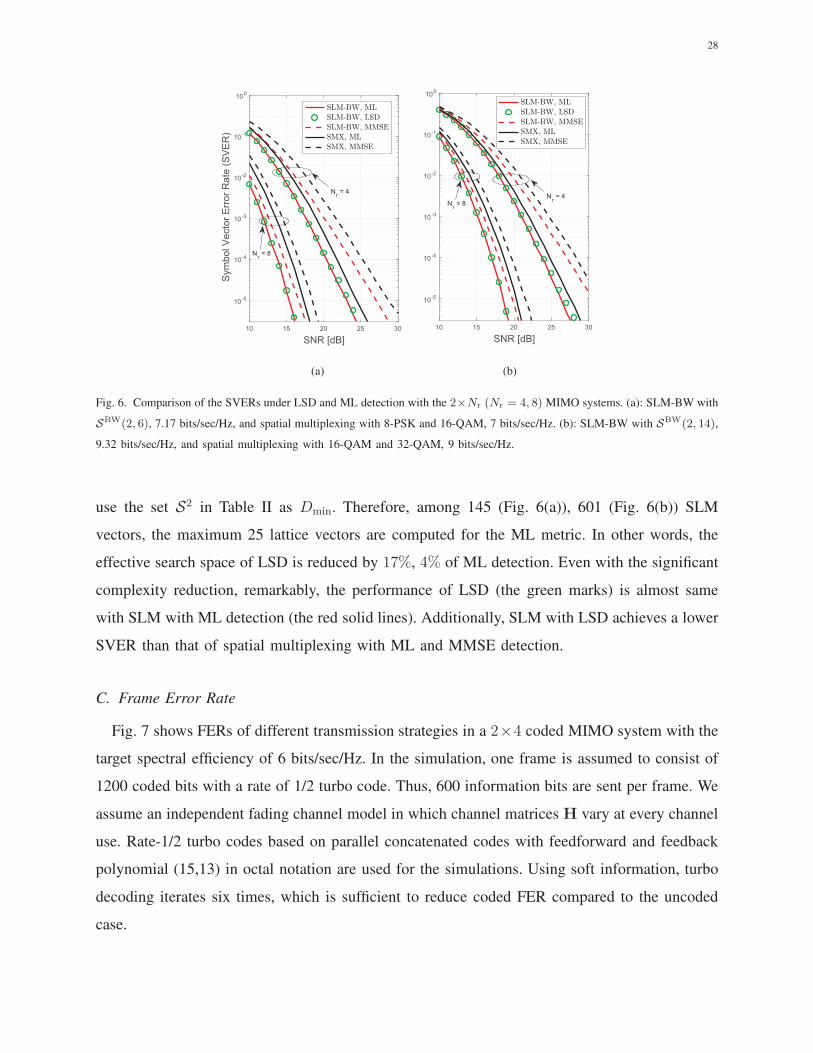
Fig. 6. Comparison of the SVERs under LSD and ML detection with the 2×Nr (Nr = 4, 8) MIMO systems. (a): SLM-BW with

SBW(2, 6), 7.17 bits/sec/Hz, and spatial multiplexing with 8-PSK and 16-QAM, 7 bits/sec/Hz. (b): SLM-BW with SBW(2, 14),

9.32 bits/sec/Hz, and spatial multiplexing with 16-QAM and 32-QAM, 9 bits/sec/Hz.

use the set S2 in Table II as Dmin. Therefore, among 145 (Fig. 6(a)), 601 (Fig. 6(b)) SLM

vectors, the maximum 25 lattice vectors are computed for the ML metric. In other words, the

effective search space of LSD is reduced by 17%, 4% of ML detection. Even with the significant

complexity reduction, remarkably, the performance of LSD (the green marks) is almost same

with SLM with ML detection (the red solid lines). Additionally, SLM with LSD achieves a lower

SVER than that of spatial multiplexing with ML and MMSE detection.

C. Frame Error Rate

Fig. 7 shows FERs of different transmission strategies in a 2×4 coded MIMO system with the

target spectral efficiency of 6 bits/sec/Hz. In the simulation, one frame is assumed to consist of

1200 coded bits with a rate of 1/2 turbo code. Thus, 600 information bits are sent per frame. We

assume an independent fading channel model in which channel matrices H vary at every channel

use. Rate-1/2 turbo codes based on parallel concatenated codes with feedforward and feedback

polynomial (15,13) in octal notation are used for the simulations. Using soft information, turbo

decoding iterates six times, which is sufficient to reduce coded FER compared to the uncoded

case.

29

0 1 2 3 4 5 6 7 8 9 10

SNR [dB]

10 -4

10 -3

10 -2

10 -1

100

Fra

me

Err

or R

ate

(FE

R)

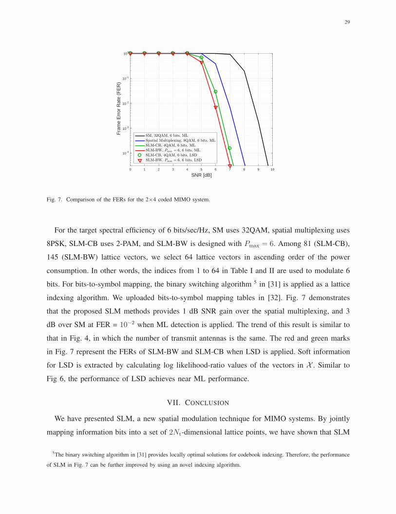
Fig. 7. Comparison of the FERs for the 2×4 coded MIMO system.

For the target spectral efficiency of 6 bits/sec/Hz, SM uses 32QAM, spatial multiplexing uses

8PSK, SLM-CB uses 2-PAM, and SLM-BW is designed with Pmax = 6. Among 81 (SLM-CB),

145 (SLM-BW) lattice vectors, we select 64 lattice vectors in ascending order of the power

consumption. In other words, the indices from 1 to 64 in Table I and II are used to modulate 6

bits. For bits-to-symbol mapping, the binary switching algorithm 5 in [31] is applied as a lattice

indexing algorithm. We uploaded bits-to-symbol mapping tables in [32]. Fig. 7 demonstrates

that the proposed SLM methods provides 1 dB SNR gain over the spatial multiplexing, and 3

dB over SM at FER = 10−2 when ML detection is applied. The trend of this result is similar to

that in Fig. 4, in which the number of transmit antennas is the same. The red and green marks

in Fig. 7 represent the FERs of SLM-BW and SLM-CB when LSD is applied. Soft information

for LSD is extracted by calculating log likelihood-ratio values of the vectors in X . Similar to

Fig 6, the performance of LSD achieves near ML performance.

VII. CONCLUSION

We have presented SLM, a new spatial modulation technique for MIMO systems. By jointly

mapping information bits into a set of 2Nt-dimensional lattice points, we have shown that SLM

5The binary switching algorithm in [31] provides locally optimal solutions for codebook indexing. Therefore, the performance

of SLM in Fig. 7 can be further improved by using an novel indexing algorithm.

30

is able to achieve the maximum spectral efficiency at high SNR under the PAM input constraint

per dimension. We also demonstrated that the SLM that uses dense Barnes-Wall lattices offers

a considerable SNR gain. We derived a tight approximation of the average mutual information

and the upper bound of average symbol-vector-error-probability and used simulations to validate

the effectiveness of our analysis. In addition, lattice sphere decoding for SLM was proposed to

diminish the detection complexity at the receiver. Simulations showed that the performance of

LSD closely matches that of ML at every SNR region with practical MIMO setups.

A promising direction for future work includes a study of impact on SLM for the case where

the number of RF chains is greater than the number of transmit antennas, i.e., Nt > NRF. Other

interesting research directions are to devise SLM techniques combined with index modulation

methods [33] for multi-carrier MIMO systems and to devise SLM techniques for the integer-

forcing framework in [34].

APPENDIX

A. Lattice Vector Quantizer

In this Appendix, we explain the lattice vector quantizers (LVQ) proposed in [29]. The LVQs

in [29] can quantize any n-dimensional vectors into Dn (D4 = ΛBW4 ) or En (E8 = ΛBW

8 )

lattices. The main advantages of these LVQs are that they can be implemented with simple

arithmetic operations and the quantization complexities follow the order of O (n). Each lattice

requires a different quantization procedure. Due to the paper limitation, we only focus on the

LVQ of Dn lattices.

Let f(xi) be the closest integer of xi. Then, for x = [x1, x2, · · · , xn]T ∈ Rn, we define f(x)

as

f(x) = [f(x1), f(x2), · · · , f(xn)]T. (63)

We also define δ(x) as the difference between x and f(x).

δ(x) = [x1 − f(x1), x2 − f(x2), · · · , xn − f(xn)]T . (64)

Using f(x) and δ(x), we define g(x) as

g(x) = [f(x1), · · · , w(xk), · · · , f(xn)]T, (65)

31

which is the same with f(x) except the k-th element w(xk), where k = argmax(|δ(x)|). The

function w(xk) rounds xk as follows:

w(xk) = f(xk) + 1, if δ(xk) ≥ 0,

= f(xk)− 1, if δ(xk) < 0. (66)

The notable fact is that the sum of all Dn lattice vectors should be even, i.e., mod(∑

i xi, 2) =

0. Therefore, we need to check whether∑

i f(xi) or∑

i g(xi) is even. Then, we admit the vector

which has even sum as the quantized output Q(x).

Example 4: Suppose x = [+1.32, − 2.51, − 0.41, + 2.70]T. Then f(x), δ(x), and g(x)

are computed as

f(x) = [+1, − 3, 0, + 3]T,

δ(x) = [+0.32, + 0.49, − 0.41, − 0.30]T,

g(x) = [+1, − 2, 0, + 3]T. (67)

Considering that∑

i f(xi) = 1 (odd) and∑

i g(xi) = 2 (even), we select g(x) as the quantized

output of x, i.e., Q(x) = g(x).

REFERENCES

[1] R. Mesleh, H. Haas, S. Sinanovic, C. W. Ahn, and S. Yun, “Spatial modulation,” IEEE Trans. Veh. Technol., vol. 57, no.

4, pp. 2228–2241, Jul. 2008.

[2] M. Di Renzo, H. Haas, and P. M. Grant, “Spatial modulation for multiple-antenna wireless systems: A survey,” IEEE

Commun. Mag., vol. 49, no. 12, Dec. 2011.

[3] M. Di Renzo, H. Haas, A. Ghrayeb, S. Sugiura, and L. Hanzo, “Spatial modulation for generalized MIMO: Challenges,

opportunities, and implementation,” Proc. IEEE, vol. 102, no. 1, pp. 56–103, Jan. 2014.

[4] P. Yang, M. Di Renzo, Y. Xiao, S. Li, and L. Hanzo, “Design guidelines for spatial modulation,” IEEE Commun. Surveys

Tuts., vol. 17, no. 1, pp. 6-26, First Quarter 2015.

[5] P. Yang, Y. Xiao, Y. L. Guan, K. Hari, A. Chockalingam, S. Sugiura, H. Haas, M. Di Renzo, C. Masouros, Z. Liu et al.,

“Single-carrier SM-MIMO: A promising design for broadband large-scale antenna systems,” IEEE Commun. Surveys Tuts.,

vol. 18, no. 3, pp. 1687-1716, Third Quarter 2016.

[6] J. Jeganathan, A. Ghrayeb, L. Szczecinski, and A. Ceron, “Space shift keying modulation for MIMO channels, IEEE Trans.

Wireless Commun., vol. 8 no. 7, pp. 3692–3703, Jul. 2009.

[7] A. Younis, N. Seramovski, R. Mesleh, and H. Haas, “Generalised spatial modulation,” in Proc. IEEE Signals, Syst. Comput.

(ASILOMAR), Pacific Grove, CA, USA, Nov. 2010, pp 1498–1502.

[8] J. Jeganathan, A. Ghrayeb, and L. Szczecinski, “Generalized space shift keying modulation for MIMO channels,” in Proc.

IEEE Int. Symp. Pers., Indoor, Mobile Radio Commun. (PIMRC), Cannes, France, Sep. 2008, pp. 1–5.

32

[9] J. Wang, S. Jia, and J. Song, “Generalised spatial modulation system with multiple active transmit antennas and low

complexity detection scheme,” IEEE Trans. Wireless Commun., vol. 11, no. 4, pp. 1605-1615, Apr. 2012.

[10] K. M. Humadi, A. I. Sulyman, and A. Alsanie, “Experimental results for generalized spatial modulation scheme with

variable active transmit antennas,” in IEEE Int. Conf. on Cognitive Radio Oriented Wireless Networks (CROWNCOM),

Doha, Qatar, April. 2015, pp. 260–270.

[11] R. Mesleh, S. S. Ikki, and H. M. Aggoune, “Quadrature spatial modulation,” IEEE Trans. Veh. Technol., vol. 64, no. 6,

pp. 2738–2742, Jun. 2015.

[12] A. A. I. Ibrahim, T. Kim, and D. J. Love, “On the achievable rate of generalized spatial modulation using multiplexing

under a Gaussian mixture model,” IEEE Trans. Commun., vol. 64, no. 4, pp. 1588–1599, Apr. 2016.

[13] N. Ma, A. Wang, C. Han, and Y. Ji, “Adaptive joint mapping generalised spatial modulation,” in IEEE Int. Conf. Commun.

in China (ICCC), China, Beijing, Aug. 2012, pp. 520–523.

[14] S. Guo, H. Zhang, S. Jin, and P. Zhang, “Spatial modulation via 3-D mapping,” IEEE Commun. Lett., vol. 20, no. 6, pp.

1096–1099, Jun. 2016.

[15] C.-C. Cheng, H. Sari, S. Sezginer, and Y. T. Su, “Enhanced spatial modulation with multiple signal constellations,” IEEE

Trans. Commun., vol. 63, no. 6, pp. 2237–2248, Jun. 2015.

[16] C.-C. Cheng, H. Sari, S. Sezginer, and Y. T. Su, “New signal designs for enhanced spatial Modulation,” IEEE Trans.

Wireless Commun., vol. 15, no. 11, pp. 7766–7777, Nov. 2016.

[17] J. Freudenberger and S. Shavgulidze, “Signal constellations based on Eisenstein integers for generalized spatial modulation,”

IEEE Commun. Lett., vol. 21, no. 3, pp. 556–559, Mar. 2017.

[18] G. D. Forney Jr. and G. Ungerboeck, “Modulation and coding for linear Gaussian channels,” IEEE Trans. Inf. Theory, vol.

44, no. 6, pp. 2384–2415, Jun. 1998.

[19] J. Conway and N. Sloane, Sphere packings, lattices and groups, Springer Science & Business Media, 2013.

[20] G. Nebe, E. M. Rains, and N. J. A. Sloane, “A simple construction of the Barnes-Wall lattices,” in Codes, Graphs, and

Systems, Springer, 2002, pp. 333–342.

[21] X. Guan, Y. Cai, W. Yang, “On the mutual information and precoding for spatial modulation with finite alphabet,” IEEE

Wireless Commun. Lett., vol. 2, no. 4, pp. 383–386, Aug. 2013.

[22] S.-R. Jin, W.-C. Choi, J.-H. Park, and D.-J. Park, “Linear precoding design for mutual information maximization in

generalized spatial modulation with finite alphabet inputs,” IEEE Commun. Lett., vol. 19, no. 8, pp. 1323–1326, Aug. 2015.

[23] S. Guo, H. Zhang, J. Zhang, and D. Yuan, “On the mutual information and constellation design criterion of spatial

modulation MIMO systems,” in Proc. IEEE Int. Conf. Commun. Syst. (ICCS), Macau, China, Nov. 2014, pp. 487–491.

[24] B. P. Buckles and M. Lybanon, “Generation of a vector from the lexicographical index,” ACM Trans. Math. Softw., vol.

3, no. 2, pp. 180-182, Jun. 1977.

[25] P. Rault and C. Guillemot, “Indexing algorithms for Zn, An, Dn, and D++n lattice vector quantizers.” IEEE Trans.

Multimedia, vol. 3, no. 4, pp. 395–404, Dec. 2001.

[26] V. Tarokh, A. Vardy, and K. Zeger, “Universal bound on the performance of lattice codes,” IEEE Trans. Inf. Theory, vol.

45, no. 2, pp. 670–681, Mar. 1999.

[27] D. Tse and P. Viswanath, Fundamentals of wireless communication, Cambridge university press, 2005.

[28] M.-S. Alouini and A. Goldsmith, “A unified approach for calculating error rates of linearly modulated signals over

generalized fading channels,” IEEE Trans. Commun., vol. 47, no. 9, pp. 1324–1334, Sept. 1999.

[29] J. Conway and N. Sloane, “Fast quantizing and decoding and algorithms for lattice quantizers and codes,” IEEE Trans.

Inf. Theory, vol.28, no. 2, pp. 227–232, Mar. 1982.

33

[30] L. Xiao et al., “Efficient compressed sensing detectors for generalized spatial modulation systems,” IEEE Trans. Veh.

Technol., vol. 66, no. 2, pp. 1284–1298, Feb. 2017.

[31] K. Zeger abd A. Gersho, “Pseudo-Gray coding,” IEEE Trans. Commun., vol. 38, pp. 2147–2158, Dec. 1990.

[32] J. Choi, Y. Nam, and N. Lee, “Bits-to-symbol mapping tables for spatial lattice modulation”, [Online]. Available:

http://wisepostech.com.

[33] E. Basar, U. Aygolu, E. Panayırcı, and H. V. Poor, “Orthogonal frequency division multiplexing with index modulation,”

IEEE Trans. Sig. Process., vol. 61, no. 22, pp. 5536–5549, Nov. 2013.

[34] J. Zhan, B. Nazer, U. Erez, and M. Gastpar, “Integer-Forcing Linear Receivers,” IEEE Trans. Inf. Theory, vol. 60, no. 12,

pp. 7661–7685, Dec. 2014.