Spatial Modelling Using a New Class of

Nonstationary Covariance Functions

Christopher J. Paciorek and Mark J. Schervish

13th June 2005

Abstract

We introduce a new class of nonstationary covariance functions for spatial modelling. Nonstationary

covariance functions allow the model to adapt to spatial surfaces whose variability changes with location.

The class includes a nonstationary version of the Matérn stationary covariance, in which the differentia-

bility of the spatial surface is controlled by a parameter, freeing one from fixing the differentiability in

advance. The class allows one to knit together local covariance parameters into a valid global nonsta-

tionary covariance, regardless of how the local covariance structure is estimated. We employ this new

nonstationary covariance in a fully Bayesian model in which the unknown spatial process has a Gaussian

process (GP) distribution with a nonstationary covariance function from the class. We model the nonsta-

tionary structure in a computationally efficient way that creates nearly stationary local behavior and for

which stationarity is a special case. We also suggest non-Bayesian approaches to nonstationary kriging.

To assess the method, we compare the Bayesian nonstationary GP model with a Bayesian stationary

GP model, various standard spatial smoothing approaches, and nonstationary models that can adapt to

function heterogeneity. In simulations, the nonstationary GP model adapts to function heterogeneity,

unlike the stationary models, and also outperforms the other nonstationary models. On a real dataset,

GP models outperform the competitors, but while the nonstationary GP gives qualitatively more sensible

results, it fails to outperform the stationary GP on held-out data, illustrating the difficulty in fitting

complex spatial functions with relatively few observations.

The nonstationary covariance model could also be used for non-Gaussian data and embedded in

additive models as well as in more complicated, hierarchical spatial or spatio-temporal models. More

complicated models may require simpler parameterizations for computational efficiency.

1

keywords: smoothing, Gaussian process, kriging, kernel convolution

1

1 Introduction

One focus of spatial statistics research has been spatial smoothing - estimating a smooth spatial process

from noisy observations or smoothing over small-scale variability. Statisticians have been interested in

constructing smoothed maps and predicting at locations for which no data are available. Two of the most

prominent approaches have been kriging and thin plate splines (see Cressie (1993, chap. 3) for a review). A

simple Bayesian version of kriging for Gaussian data can be specified as

Yi ∼ N(f(xi), η2)

f(·) ∼ GP (µ,C(·, ·; θ)) , (1)

where η2 is the noise variance and f(·) is the unknown spatial process with a Gaussian process (GP) prior

distribution, whose covariance function, C(·, ·; θ), is parameterized by θ. This model underlies the stan-

dard kriging approach, in which C(·; θ) is a stationary covariance, with the covariance between the function

values at any two points a function of Euclidean distance (or possibly a more general anisotropic or Maha-

lanobis distance). The low-dimensional θ is generally estimated using variogram techniques (Cressie 1993,

chap. 2) or by maximum likelihood (Smith 2001, p. 66). The spatial process estimate is the posterior mean

conditional on estimates of µ, η, and θ. While various approaches to kriging and thin plate spline models

have been used successfully for spatial process estimation, they have the weakness of being global models,

in which the variability of the estimated process is the same throughout the domain because θ applies to the

entire domain.

This failure to adapt to variability, or heterogeneity, in the unknown process is of particular importance

in environmental, geophysical, and other spatial datasets, in which domain knowledge suggests that the

1Christopher Paciorek is Research Fellow, Department of Biostatistics, Harvard School of Public Health, Boston, MA 02115 (E-

mail: paciorek@alumni.cmu.edu). Mark Schervish is Professor, Department of Statistics, Carnegie Mellon University, Pittsburgh,

PA 15213 (E-mail: mark@stat.cmu.edu). An earlier version of this work was part of the first author’s doctoral thesis at Carnegie

Mellon University. The authors thank Doug Nychka for helpful comments.

2

function may be nonstationary. For example, in mountainous regions, environmental variables are likely to

vary much more quickly than in flat regions. Spatial statistics researchers have made some progress in defin-

ing nonstationary covariance structures; in particular, this work builds on Higdon, Swall, and Kern (1999),

who convolve spatially-varying kernels to give a nonstationary version of the squared exponential stationary

covariance. Fuentes and Smith (2001) and Fuentes (2001) have an alternative kernel approach in which the

unknown process is taken to be the convolution of a fixed kernel over independent stationary processes with

different covariance parameters; Barber and Fuentes (2004) give a discretized mixture version of the model.

Wood, Jiang, and Tanner (2002) estimate the spatial process as a mixture of thin plate splines to achieve

nonstationarity. The spatial deformation approach attempts to retain the simplicity of the stationary covari-

ance structure by mapping the original input space to a new space in which stationarity can be assumed

(Sampson and Guttorp 1992; Damian, Sampson, and Guttorp 2001; Schmidt and O’Hagan 2003). Research

on the deformation approach has focused on multiple noisy replicates of the spatial function rather than the

setting of one set of observations on which we focus here.

Many nonparametric regression methods are also applicable to spatial data, but spatial modelling re-

quires flexible two-dimensional surfaces, while many nonparametric regression techniques focus on addi-

tive models, summing one-dimensional curves. In particular, while Bayesian free-knot spline models, in

which the number and location of the knots are part of the estimation problem, have been very successful in

one dimension (DiMatteo, Genovese, and Kass 2001), effectively extending splines to higher dimensions is

more difficult. Using different bases, Denison, Mallick, and Smith (1998) and Holmes and Mallick (2001)

fit free-knot spline models for two and higher dimensions using reversible-jump MCMC. Lang and Brezger

(2004) and Crainiceanu, Ruppert, and Carroll (2004) use penalized splines with spatially-varying penalties

in two dimensions. While not commonly used for spatial data, neural network models can adapt to function

heterogeneity (Neal 1996). Tresp (2001) and Rasmussen and Ghahramani (2002) use mixtures of stationary

GPs; they show success in one dimension, but do not provide results in higher dimensions nor compare their

model to other methods.

In this work, we extend the Higdon et al. (1999) nonstationary covariance function to create a class of

closed-form nonstationary covariance functions, including a Matérn nonstationary covariance, parameter-

ized by spatially-varying covariance parameters (Section 2). We demonstrate how this covariance can be

used in an ad hoc nonstationary kriging approach (Section 3.1) and in a fully Bayesian GP spatial model

3

(Section 3.2). We compare the performance of the nonstationary GP model to a range of spatial models on

simulated and real datasets (Sections 4 and 5). We conclude by suggesting strategies for improving compu-

tational efficiency and and discussing the use of the nonstationary covariance in more complicated models

(Section 6).

2 A new class of nonstationary covariance functions

In this section we extend the nonstationary covariance of Higdon et al. (1999), providing a general class of

closed-form nonstationary covariance functions built upon familiar stationary covariance functions. The ap-

proach constructs a global covariance by knitting together local covariance structures and is valid regardless

of how the local covariance parameters are estimated.

2.1 Review of stationary covariance functions

The covariance function is crucial in GP modelling; it controls how the observations are weighted for spa-

tial prediction. Recent work in spatial statistics has focused on the Matérn covariance, whose stationary,

isotropic form is

C(τ) = σ2 1

Γ(ν)2ν−1

(

2√ντ

ρ

)ν

Kν

(

2√ντ

ρ

)

, ρ > 0; ν > 0

where τ is distance, ρ is the spatial range parameter, and Kν(·) is the modified Bessel function of the

second kind, whose order is the differentiability parameter, ν. The behavior of the covariance function of a

stochastic process near the origin determines the smoothness properties of sample functions (Abrahamsen

1997; Stein 1999; Paciorek 2003, chap. 2). The Matérn form has the desirable property that sample functions

of Gaussian process distributions with this covariance are dν − 1e times differentiable. As ν → ∞, the

Matérn approaches the squared exponential (also called the Gaussian) form, popular in machine learning,

whose sample functions are infinitely differentiable. For ν = 0.5, the Matérn takes the exponential form,

which is popular in spatial statistics, but produces continuous but non-differentiable sample functions, which

seems insufficiently smooth for many applications. While it is not clear that sample function differentiability

can be estimated from data, having the additional parameter, ν, allows one to choose from a wider range of

sample path behavior than the extremes of the exponential and squared exponential covariances provide, or,

if estimated, may allow for additional flexibility in spatial modelling. For example, the smoothing matrices

4

produced by the exponential and Matérn (ν = 4) correlation functions are rather different, as are sample

path realizations.

Stationary, isotropic covariance functions can be easily generalized to anisotropic covariance functions

that account for directionality by using Mahalanobis distance,

τ(xi,xj) =√

(xi − xj)T Σ−1(xi − xj), (2)

where Σ is an arbitrary positive definite matrix, rather than Σ = I , which gives Euclidean distance and

isotropy. The nonstationary covariance function we introduce next builds on this more general anisotropic

form.

2.2 From stationarity to nonstationarity via kernel convolution

Higdon et al. (1999) introduced a nonstationary covariance function obtained by convolving kernel func-

tions, CNS(xi,xj) =∫

<2 Kxi(u)Kxj

(u)du, where xi, xj , and u are locations in <2, and Kx(·) is a

kernel function centered at x. They motivate this construction as the covariance function of a process, f(·),

f(x) =

∫

<2

Kx(u)ψ(u)du, (3)

produced by convolving a white noise process, ψ(·), with the spatially-varying kernel function. One can

avoid the technical details involved in carefully defining such a white noise process by using the definition

of positive definiteness to show directly that the covariance function is positive definite in every Euclidean

space, <p, p = 1, 2, . . .:

n∑

i=1

n∑

j=1

aiajCNS(xi,xj) =

n∑

i=1

n∑

j=1

aiaj

∫

<PKxi

(u)Kxj(u)du

=

∫

<P

n∑

i=1

aiKxi(u)

n∑

j=1

ajKxj(u)du

=

∫

<P

(

n∑

i=1

aiKxi(u)

)2

du ≥ 0. (4)

Note that the kernel function is arbitrary; positive definiteness is achieved because the kernel at a location

provides all the information about how the location affects the pairwise correlations involving that location.

For Gaussian kernels (taking Kx(·) to be a (multivariate) Gaussian density centered at x), one can show

5

using convolution (Paciorek 2003, sec. 2.2) that the nonstationary covariance function takes the simple

form,

CNS(xi,xj) = σ2|Σi|1

4 |Σj |1

4

∣

∣

∣

∣

Σi + Σj

2

∣

∣

∣

∣

−1

2

exp (−Qij) , (5)

with quadratic form

Qij = (xi − xj)T(

Σi + Σj

2

)−1

(xi − xj), (6)

where Σi = Σ(xi), which we call the kernel matrix, is the covariance matrix of the Gaussian kernel at

xi. (5) has the form of an anisotropic squared exponential correlation function, but in place of a spatially

constant matrix, Σ (which gives stationarity and anisotropy), in the quadratic form (2), we average the kernel

matrices for the two locations (6). Gibbs (1997) derived a special case of (5) in which the kernel matrices

are diagonal. The evolution of the kernel matrices in the domain produces nonstationary covariance, with

kernels with small variances, and therefore little overlap with kernels at other locations, producing locally

short correlation scales. Unfortunately, so long as the kernel matrices vary smoothly in the input space,

sample functions from GPs with the covariance (5) are infinitely differentiable (Paciorek 2003, chap. 2),

just as for the stationary squared exponential. Stein (1999) discusses in detail why such highly smooth paths

are undesirable and presents an asymptotic argument for using covariance functions in which the smoothness

is allowed to vary.

2.3 Generalizing the kernel convolution form

To create a more general form than the squared exponential, we construct a class of covariance functions,

substituting√

Qij in place of τ/ρ in stationary correlation functions. Unfortunately, since√

Qij is not a

distance metric, it violates the triangle inequality, so this cannot be done arbitrarily, but it can be done for a

class of stationary correlation functions; the proof of the theorem is given in the Appendix.

Theorem 1 If an isotropic correlation function, RS(τ), is positive definite on <p for every p = 1, 2, . . .,

then the function, RNS(·, ·), defined by

RNS(xi,xj) = |Σi|1

4 |Σj |1

4

∣

∣

∣

∣

Σi + Σj

2

∣

∣

∣

∣

−1

2

RS(√

Qij

)

(7)

with√

Qij used in place of τ , is a nonstationary correlation function, positive definite on <p, p = 1, 2, . . ..

6

The result applies to correlation functions that are positive definite in Euclidean space of every dimension,

in particular the power exponential, rational quadratic, and Matérn correlation functions.

Under conditions that ensure that the elements of the kernel matrices vary smoothly over the domain, the

mean square and sample path differentiability of Gaussian processes parameterized by covariance functions

of the form (7) follow from the differentiability properties of Gaussian processes parameterized by the

underlying stationary covariance function (Paciorek 2003, chap. 2). The precise statement of the theorems

and proofs behind this result are involved and not the focus of this paper. However, the result is intuitive

and best made clear as follows. If the elements of the kernel matrices vary smoothly (see Section 3.2.1 for

such a construction), then in a small neighborhood of x0, the covariance structure is essentially constant,

Σ(x) ≈ Σ(x0), so the differentiability properties, which depend on the behavior of the covariance near the

origin, are the same as those for the underlying stationary covariance.

The new class of nonstationary covariance functions includes a nonstationary version of the Matérn

correlation function,

RNS(xi,xj) =1

Γ(ν)2ν−1|Σi|

1

4 |Σj |1

4

∣

∣

∣

∣

Σi + Σj

2

∣

∣

∣

∣

−1

2(

2√

νQij

)νKν

(

2√

νQij

)

, (8)

which includes a nonstationary version of the exponential correlation as the special case when ν = 0.5.

As with the stationary form, the sample function differentiability of Gaussian processes with nonstationary

Matérn covariance increases with ν. Another form is the rational quadratic correlation function,

RNS(xi,xj) = |Σi|1

4 |Σj |1

4

∣

∣

∣

∣

Σi + Σj

2

∣

∣

∣

∣

1

2

(

1

1 +Qij

)ν

,

a correlation function with a long tail. In the remainder of the paper, we focus on the nonstationary Matérn

form.

3 Implementation of the new nonstationary covariance

3.1 Ad hoc nonstationary kriging

The kernel convolution nonstationary covariance provides a way to construct closed-form covariance func-

tions based on stationary correlation forms and local covariance parameters. One advantage of our approach

7

is that construction using arbitrary local parameters is positive definite. The nonstationary covariance struc-

ture is highly parameterized relative to a stationary covariance structure, so optimization is difficult and

runs the danger of overfitting. In this section, we propose approaches by which the nonstationary covari-

ance (7) can be used in a kriging framework, estimating the covariance structure and then fitting the surface

conditional on that structure.

3.1.1 Methods for estimating the nonstationary covariance structure

When distinct regions are present, one can piece together regional stationary covariances. The parameters

of regional anisotropic covariances could be estimated using either a variogram fitting approach or marginal

likelihood maximization in which only the data in a region are used to estimate the region-specific parame-

ters. Then, to knit together a full covariance for the entire domain, set Σi = ΣR(i), where R(i) denotes the

region in which location i falls and ΣR(i) is constructed for each region from the parameters, θR(i), of the

anisotropic correlation structure estimated for the region. One can use different values for σ, µ, and η for

the different regions. One could also use different values of ν, following Stein (2005), who has extended

our approach to allow for spatially-varying ν. In the next section, we illustrate this approach in Colorado,

splitting the state into two regions of differing topography.

Another possibility is to estimate the kernel matrices at each location of interest in a weighted or moving

window fashion. Recall that if the elements of the kernel matrices vary slowly, the nonstationary covariance

is locally a nearly stationary anisotropic covariance. In a small neighborhood, for xj near xi, Σj ≈ Σi; our

task is to estimate the parameters, θi, of an anisotropic covariance, from which the kernel matrix, Σi, will

be constructed. To estimate θi based on the variogram, we could use a moving window to include in the

empirical variogram only pairs of locations for which either one or both of the locations are near xi. One

could also assign weights to each pair of locations and estimate θi based on weighted variograms. Such a

fitting approach is similar to that of Barber and Fuentes (2004), who fit local variograms to time-replicated

data, demonstrating the advantage of having replicated data. To estimate θi using the marginal likelihood

approach, one could use the marginal likelihood only for observations from locations near xi. Doing this

for each location allows us to create spatially-varying kernel matrices, Σi.

Finally, one might parameterize the nonstationary covariance as a function of key covariates to reduce

8

the dimension of the estimation problem. For example, in the Colorado precipitation example in the next

section, one might specify the correlation range to be a simple parameterized function of local elevation

heterogeneity.

The spatial process at observation and prediction locations can then be estimated using the mean and

variance conditional on the nonstationary covariance structure constructed from the estimated kernel matri-

ces, using standard multivariate Gaussian conditional calculations (Paciorek 2003, sec. 1.3). Note that for

prediction, we need to estimate kernel matrices for the prediction locations using covariance information

based on nearby observation locations.

3.1.2 Illustration

Climatological data for Colorado provide a nice illustration of a simple application of nonstationary krig-

ing. To first approximation, Colorado is divided into a mountainous western portion, west of Denver

and the I-25 corridor, and a flat plains portion in the east (Fig. 1). The Geophysical Statistics Project

at the National Center for Atmospheric Research (http://www.cgd.ucar.edu /stats /Data

/US.monthly.met) has posted a useful subset of the United States climate record over the past cen-

tury from a large network of weather stations. Areas of complex topography are a particular challenge for

making predictions off the observation network, and even for the continental U.S. the observation record

is quite sparse relative to the resolution needed for understanding impacts of changing climate. For this

illustration, we take the log-transformed annual precipitation in Colorado for 1981, the year for which the

most stations without any missing monthly values (217) were available, and compare kriging with model

(1) using both stationary and nonstationary covariances.

For stationary kriging, we use a Matérn covariance with anisotropic distance (2), where Σ = ΓΛΓT ,

with Γ an eigenvector (rotation) matrix parameterized by Givens angle ψ, and Λ a diagonal eigenvalue

matrix with eigenvalues (squared correlation range parameters), ρ21 and ρ2

2. After integrating the spatial

function values at the observation locations out of the model, we estimate the parameters, η, σ, ρ1, ρ2, ψ,

by maximizing the resulting marginal likelihood using the nlm() function in R. We fix the process mean,

µ = y, and ν = 4.

For nonstationary kriging, we fit separate anisotropic covariance structures in the eastern and western

9

regions, split at longitude 104.873 W, by maximizing the marginal likelihoods for each region with respect

to the parameters. We again estimate µ = y, shared by the regions, and fix ν = 4. We construct the Matérn

nonstationary covariance structure (8) for the entire dataset by setting Σi = Σ(θR(i)), where θR(i) =

ρ1,R(i), ρ2,R(i), ψR(i).

Table 1 shows the parameter estimates for the two models. As expected for the nonstationary model,

because of the topographical variability in western Colorado, the correlation ranges are much smaller than

in eastern Colorado, and the estimate of the function variability, σ, is larger. The similarity of the western

estimates with the statewide stationary estimates suggests that the stationary estimates are driven by the

more variable western data. The corresponding nonstationary surface estimate shows more heterogeneity in

the west than the east (Fig. 2). The standard deviations of the estimated surface for the nonstationary kriging

model demonstrate much more certainty about the surface values in the east, as expected (Fig. 2c,d). In the

west, the complexity of the surface results in high levels of uncertainty away from the observation locations,

as is the case throughout the state in the stationary approach. Both approaches estimate 137 degrees of

freedom for the surface, based on the trace of the smoothing matrix, and since the nonstationary kriging

model has a much higher log likelihood (181 compared to 143), both AIC and BIC decisively favor the

nonstationary kriging model.

One drawback to having sharply delineated regions is seen in the sharp changes at the border between

the regions (Fig. 2b,d). This occurs because the kernels change sharply at the border (see Gibbs (1997) and

Paciorek (2003, sec. 2.2) for discussion of this effect). One simple way to remove this discontinuity would

be to smooth the covariance parameters, and therefore the resulting kernel matrices, in the vicinity of the

boundary. A more principled approach is a fully Bayesian model, in which the kernels are constrained to

vary smoothly, minimizing the effect, as seen in Section 5.3.1.

3.2 A hierarchical Bayesian model for spatial smoothing

The nonstationary kriging approach suffers from several drawbacks. First, the ad hoc estimation of the

covariance structure depends on how one estimates the local covariance parameters; in the illustration this

involved how to split the area into regions. Second, as for kriging in general, uncertainty in the covariance

structure is not accounted for; in the case of nonstationary covariance with its more flexible form and larger

10

number of parameters, this uncertainty is of much more concern than in the stationary case. To address

these concerns, we construct a fully Bayesian model, with prior distributions on the kernels that determine

the nonstationary covariance structure.

3.2.1 Basic Bayesian model

The Bayesian model starts with the basic kriging setup (1) and sets C(·, ·; θ) = σ2fR

NSf (·, ·; Σ(·), νf ),

where RNSf is the nonstationary Matérn correlation function (8) constructed from Σ(·), the kernel matrix

process, described below. For the differentiability parameter, we use the prior, νf ∼ U(0.5, 30), which

produces sample paths that vary between non-differentiable (0.5) and highly differentiable. We use proper,

but diffuse, priors for µf , σ2f , and η2, and bound σ2

f based on the range of the observation values. The

main challenge is to parameterize the kernels (see MacKay and Takeuchi (1995) for a discussion of the

difficulties), since their evolution over space determines how quickly the covariance structure changes over

the domain and therefore the degree to which the model adapts to heterogeneity in the unknown function.

In many problems, it seems natural that the covariance structure would evolve smoothly, as parameterized

below.

The kernel matrix process, Σ(·), is parameterized as follows. Each location, xi, has a Gaussian kernel

with mean xi and covariance (kernel) matrix, Σi = Σ(xi). Since there are (implicitly) kernel matrices at

each location in space, we have a multivariate process, the matrix-valued function, Σ(·). First, construct

an individual kernel matrix using the spectral decomposition, Σi = ΓiΛiΓTi where Λi is a diagonal matrix

of eigenvalues, λ1(xi) and λ2(xi), and Γi is an eigenvector matrix constructed as described below from

γ1(xi) and γ2(xi). We construct Σ(·) over the entire space, ensuring that each Σ(xi) is positive definite, by

creating spatial hyperprocesses, λ1(·), λ2(·), γ1(·), and γ2(·). We will refer to these as the eigenvalue and

eigenvector processes, and to them collectively as the eigenprocesses. Let φ(·) ∈ log(λ2(·)), γ1(·), γ2(·)denote any one of these eigenprocesses; λ1(·) is derived from γ1(·) and γ2(·). We take each φ(·) to have

a stationary GP prior with anisotropic Matérn correlation function (Section 3.2.2); this parameterization of

the processes ensures that the kernel matrices vary smoothly in an elementwise fashion by forcing their

eigenvalues and eigenvectors to vary smoothly. Parameterizing the eigenvectors of the kernel matrices using

a spatial process of Givens angles, with an angle at each location, is difficult because the angles have range

11

[0, 2π) ≡ S 1, which is not compatible with the range of a GP. Instead, Γi is constructed from the eigenvector

processes,

Γi =

γ1(xi)di

−γ2(xi)di

γ2(xi)di

γ1(xi)di

,

where di =√

γ21(xi) + γ2

2(xi). In turn, λ1(xi) is taken to be d2i , the squared length of the eigenvector

constructed from γ1(xi) and γ2(xi).

An alternative to the eigendecomposition parameterization is to represent the Gaussian kernels as el-

lipses of constant probability density, parameterized by the focus and size of the ellipse, and to have the

focal coordinates and ellipse sizes vary smoothly over space (Higdon et al. 1999). However, Higdon et al.

(1999) fixed the ellipse size at a constant value common to all locations, and Swall (1999, p. 94) found

overfitting and mixing problems when the ellipse size was allowed to vary, although we also noticed slow

mixing in our parameterization. Also, the eigendecomposition approach extends more readily to higher

dimensions, which may be of interest for spatial data in three dimensions and more general nonparametric

regression problems (Paciorek and Schervish 2004).

3.2.2 Representation of stationary GPs in the hierarchy

One can represent the stationary GPs used to construct the nonstationary covariance structure in a straight-

forward way, working with the Cholesky decompositions of the covariance matrices for each of the pro-

cesses (Paciorek 2003, chap. 3; Paciorek and Schervish 2004), but the MCMC computations are slow.

Instead, we represent each using a basis function approximation to a stationary GP, following Kammann

and Wand (2003). The vector of values of the spatial process, φ(·), at the observation locations, φ =

φ(x1), . . . , φ(xn), is a linear combination of basis functions,

φ = µφ + σφZφuφ, (9)

Zφ = ΨφΩ−

1

2

φ .

The basis matrix, Zφ, is constructed using radial (i.e., isotropic) basis functions, where Ψφ contains pair-

wise Matérn covariances, C(·; ρφ, νφ), between the observation locations and pre-specified knot locations,

κk, k = 1, . . . ,K, while Ω−1/2φ is calculated by singular value decomposition from a similar matrix with

12

pairwise covariances amongst the knot locations. Knots at all the data locations would give an exact rep-

resentation of a stationary GP. Prediction for φ(·) uses Ψ∗φ, which is calculated based on the covariances

between the prediction locations and the knots. We use a relatively coarse 8 by 8 grid of K = 64 knots,

because the eigenprocesses are in the hierarchy of the model and we do not expect them to be very variable.

To limit the number of parameters involved, we place some constraints on the hyperparameters of the

stationary GPs, while still allowing the eigenprocesses to be flexible. In particular, we fix σ2φ, letting the

variability of the GP be determined by ρφ (see Zhang (2004) for asymptotic justification). Since we are

working in geographic space, in which distances in different directions are measured in the same units, for

the eigenvector processes, we use a single ργ as a correlation scale common to the two processes, but to

allow sufficient potential heterogeneity in the eigenvectors, we use separate parameters, µγ1and µγ2

, and

coefficients, uγ1and uγ2

, for the two eigenvector processes. For all of the eigenprocesses, we fix ν = 5,

because it should have minimal impact on the spatial surface estimate and is not well-informed by the

data. We take uφ ∼ N(0, I) and use vague but proper priors for the free hyperparameters, with boundary

constraints on the µφ and ρφ parameters to prevent the Markov chain from getting stuck in regions with a

flat likelihood.

Since it is difficult to encapsulate prior knowledge about the spatial surface directly into the GP priors

for the eigenprocesses, one could also place an additional prior on the complexity of the posterior mean

spatial surface, conditional on the covariance structure and other parameters. This can be estimated by the

trace of the smoothing matrix,

df = tr(

Cf (Cf + Cy)−1)

+ 1

(Hastie and Tibshirani 1990, p. 52), adding one to account for the degree of freedom used to estimate µf .

Our results are not based on this additional prior, because the nonstationary model did not tend to use more

df than the stationary model, presumably because of the natural Bayesian penalty on model complexity

(Denison, Holmes, Mallick, and Smith 2002, p. 20).

13

3.2.3 MCMC sampling

One can integrate f , the spatial process evaluated at the observation locations, out of the GP model, leaving

a marginal posterior whose marginal likelihood is,

Y ∼ N(µf , σ2fR

NSf + η2I), (10)

where RNSf is the nonstationary covariance matrix of the spatial process at the observation locations. In the

stationary GP model, the marginal posterior contains a small number of hyperparameters to either optimize

or sample via MCMC. In the nonstationary case, the dependence of RNSf on the kernel matrices precludes

straightforward optimization; instead we use MCMC. We sample the parameters at the first level of the prior

hierarchy, µf , σf , νf , and η, via Metropolis-Hastings. Sampling the eigenprocesses and their hyperparam-

eters is more involved. For a given eigenprocess, φ(·) ∈ log(λ2(·)), γ1(·), γ2(·), we choose to sample,

via Metropolis-Hastings, µφ, ρφ, and (as a vector) uφ. φ is not sampled directly, but is determined by the

representation (9), thereby involving the eigenprocess hyperparameters directly in the marginal likelihood

through their effect on φ and therefore onRNSf in (10). This is analogous to the uncentered parameterization

discussed in Gelfand, Sahu, and Carlin (1996), in contrast to the centered parameterization, which in this

case would involve sampling φ rather than uφ and in which acceptance of hyperparameter proposals would

depend only on their priors and the GP distributions of the eigenprocesses. In our experience, the uncentered

approach, in which the hyperparameters are informed directly by the data, mixes faster than the centered

approach. Christensen, Roberts, and Sköld (2003) discuss on-the-fly reparameterizations, but their focus

is on spatial processes that determine mean structure, unlike this situation in which the eigenprocesses are

involved in parameterizing the nonstationary covariance structure. Furthermore their reparameterizations

are computationally intensive and may involve numerical computations with numerically singular matrices

when the Matérn covariance is used.

Note that in sampling the spatial process conditional on the nonstationary covariance, pivoting (e.g.,

see the R chol() function) is sometimes necessary because the conditional posterior variance is numerically

singular.

14

4 Simulations

We compare the performance of the nonstationary GP model to several alternatives, most importantly a

stationary GP model, on two simulated datasets. The first dataset is a stationary function, with similar vari-

ability throughout the domain, while the second is a nonstationary function. The first group of alternatives

includes standard methods that can be easily performed in R, most using library functions. The second

group comprises Bayesian methods that in theory can adapt to heterogeneity in the function by sampling the

basis functions within the MCMC.

4.1 Alternative methods

The abbreviations used in the results are given parenthetically here in the text. The Bayesian nonstationary

GP model is abbreviated ‘nsgp’.

4.1.1 Standard spatial methods

The first method (sgp) is a stationary, anisotropic version of the nonstationary Bayesian GP model. After in-

tegrating the spatial process values at the training locations out of the model, the parameters, µ, η, σ, ρ1, ρ2, ψ, ν,

are sampled via MCMC. The second method (krig) is likelihood-based kriging as described in Section 3.1.2,

but we also estimate ν in the numerical optimization. The third method (tps) fits the surface as a thin plate

spline (Green and Silverman 1994), using the Tps() function in the fields library in R, in which the smooth-

ing parameter is chosen automatically by generalized cross-validation (GCV). The fourth method (gam)

also fits the spatial surface using a thin plate spline and GCV, but in a computationally efficient way (Wood

2003), coded in the gam() function in the mgcv library in R. One advantage of gam() over Tps() that arises in

applications is that gam() allows the inclusion of additional covariates, including additional smooth terms,

using an algorithm that can optimize multiple penalty terms (Wood 2000). Since these methods all rely on

a small number of smoothing parameters/penalty terms that do not vary with location, none are designed

to handle nonstationarity. Also note that only the kriging and the stationary Bayesian GP approaches are

designed to handle anisotropy.

15

4.1.2 Nonparametric regression models

There are many nonparametric regression methods, with much work done in the machine learning litera-

ture as well as by statisticians. These methods can be used for spatial smoothing; we restrict our attention

to a small number of methods with readily available code. Other potential methods include wavelet mod-

els, mixtures of GPs or thin plate splines, and regression trees. The first two methods are free-knot spline

models that, by allowing the number and location of the knots to change during the fitting procedure, can

model nonstationarity. Denison et al. (1998) created a Bayesian version of the MARS algorithm (Fried-

man 1991), which uses basis functions that are tensor products of univariate splines in the truncated power

basis, with knots at the data points. The second method (mls) uses free-knot multivariate linear splines

(MLS) where the basis functions are truncated linear planes, which gives a surface that is continuous but

not differentiable where the planes meet (Holmes and Mallick 2001). In the simulations and case study,

we report numerical results only for the MLS basis, because it performed better than the MARS basis. The

final method (nn) is a neural network model, in particular a multilayer perceptron with one hidden layer,

with the spatial surface modelled asf(x) = β0 +∑K

k=1 βkgk

(

uTkx)

, where the gk(·) functions are tanh

functions and the uk parameters determine the position and orientation of the basis functions. This is very

similar to the MLS model, for which gk(·) is the identity function. We use the Bayesian implementation of

R. Neal (http://www.cs.toronto.edu /~radford /fbm.software.html) to fit the model,

fixing K = 50 (K = 200 for the case study) to allow for a sufficiently flexible function but minimize

computational difficulties.

4.2 Datasets

The first dataset is a two-dimensional test function first introduced by Hwang, Lay, Maechler, Martin, and

Schimert (1994),

f(x1, x2) = 1.9 · (1.35 + exp(x1) sin(13 · (x1 − .6)2) exp(−x2) sin(7x2)).

The variability of this function is similar throughout the domain (Fig. 3a), allowing us to compare the various

methods on a dataset for which stationary models should perform well. We use 225 training locations and

400 fixed test locations, taken on an equally spaced grid over the domain [0, 1]2. We simulate 50 samples

16

of noisy Gaussian data (η = 0.25) from the true function, each using a different sample of 225 training

locations from a uniform distribution over the domain. Test observations at the 400 test locations are sampled

anew for each of the 50 samples for use in evaluation.

The second dataset is designed to see how well the methods do in fitting a heterogeneous function

(Figure 3b),

f(x1, x2) = sin1

x1x2.

We use 250 training locations and 400 test locations on an equally spaced grid over the domain, [0.3, 1]2. 50

Gaussian data samples (η = 0.3) are drawn as in the first dataset.

4.3 Evaluation criteria

For the simulated data, we use several criteria to assess the quality of fit based on the known spatial surface.

The first criterion assesses just the fitted surface, using the standardized mean squared error (also called

the fraction of variance unexplained (FVU)) of the estimated surface (the posterior mean for the Bayesian

models), MSEsim =∑M

m=1(fm − fm)2/∑M

m=1(fm − ¯f)2, where fm (fm) is the true (estimated) surface

at x∗

m, taken over a grid of test locations, xm∗, m = 1, . . . ,M . The next measure assesses point estimates

of both the surface values and error variance using the predictive density of test data, h(y∗|·). We scale

the estimated predictive density relative to the true density of the test data using Kullback-Leibler (KL)

divergence. The expectation involved in KL is taken over the true density of observations, y∗m, at location

m, and averaged over the grid of test locations,

KLsim,point =1

M

M∑

m=1

∫

logh(y∗m|fm, η)

h(y∗m|fm, η)h(y∗m|fm, η)dy

∗m

= − logη

η− 1

2+

η2

2η2+

1

M

∑Mm=1(fm − fm)2

2η2

where η (η) is the true (estimated) error standard deviation. Smaller divergences indicate better fits. With

the Bayesian methods, as a third criterion, we can also calculate the KL divergence using the full posterior,

estimated by averaging over the MCMC samples, t = 1, . . . , T . We assess the fit for an entire test sample,

y∗, and scale by M,

KLsim,Bayes =1

M

∫

logh(y∗|f , η)h(y∗|y)

h(y∗|f , η)dy∗ (11)

17

≈ 1

Mlog

h(y∗|f , η)h(y∗|y)

(12)

=1

Mlog

h(y∗|f , η)∫

h(y∗|f, η)Π(f, η|y)dfdη

≈ − log η − 1

2Mη2

M∑

m=1

(y∗m − fm)2 − 1

Mlog

1

T

T∑

t=1

1

ηM(t)

exp

(

− 1

2η2(t)

M∑

m=1

(y∗m − fm,(t))2

)

.

Ideally, this should be done by averaging over many samples of test data (to approximate the integral in (11)),

y1∗, . . . ,yJ

∗, for J large, but we use only one for computational convenience (12). In place of averaging

over many test samples with the same training sample, we average over repeated training and test samples

by fitting the models to the 50 replicated data samples. For all three criteria, we restrict attention to those

test locations within the convex hull of each of the 50 samples of training data, allowing us to ignore the

effects of extrapolation.

For the Bayesian methods, adequate mixing and convergence are important and determine the number of

MCMC samples needed and therefore the computational speeds of the methods. We compare the iterations

of the sample log posterior density (Cowles and Carlin 1996) and key parameters between the methods to

get a general sense for how many iterations each needs to run, examining the autocorrelation and effective

sample size (Neal 1993, p. 105),

ESS =T

1 + 2∑

∞d=1 ρd(θ))

,

where T is the number of MCMC samples and ρd(θ) is the autocorrelation at lag d for the quantity/parameter

θ.

4.4 Results

For the stationary simulated dataset, the various criteria paint similar pictures (Fig. 4a-4c). Likelihood-based

kriging and the Bayesian GP methods perform best, outperforming standard stationary approaches and the

non-GP Bayesian nonstationary methods. As a rough measure of whether the signal to noise ratio in 50

simulations is strong enough to draw firm conclusions, we calculate p-values using paired t-tests to compare

the nonstationary GP with the other methods, ignoring the issue of multiple comparisons. The nonstationary

GP is significantly better (p < 1i10 −14), based on paired t-tests, than the thin plate spline, GAM, and MLS

models on all criteria, while not significantly different than the stationary GP model. It is not significantly

18

different from the kriging model on MSE and point KL and significantly worse (p = 0.02) on the Bayes

KL, while being significantly better than the neural network model on MSE (p = 1 i 10 −10) and point KL

(p = 1 i 10 −4) and marginally worse on Bayes KL (p = 0.054). It is not surprising that the nonstationary

GP model is no better than the stationary model, but their equivalent performance is encouraging given that

the nonstationary model is so highly-parameterized.

On the nonstationary simulated dataset, the nonstationary GP model, outperforms the stationary ap-

proaches on the various criteria, as expected, as well as the other nonstationary methods on most criteria

(Fig. 4d-4f). The nonstationary GP is significantly better than the stationary methods (p < 1 i 10 −12) and

significantly better than the MLS or neural network models (p < 0.0067) on all criteria, except that there is

no significant difference between the nonstationary model and the neural network on the Bayes KL.

Results are similar when the full grid of test locations, including points outside the convex hull of the

training data, is used, although the MLS model performs poorly outside the hull and the neural network

model degrades there as well. We have not reported results from the MARS model because it performs

poorly, particularly outside the convex hull.

Mixing of the nonstationary model is relatively slow, but it appears that adequate mixing on relatively

simple nonstationary data such as these simulations can be achieved with runs of tens of thousands of

iterations. Based on a run of 3000 iterations for the stationary model (coded in R, this took 6 hours on a

3.06Ghz Intel Xeon (32 bit) processor running Linux) and 5000 for the nonstationary model (19 hours), with

every tenth iteration saved, the effective sample size based on the log posterior was 104 for the stationary

model and 29 (19 based on only the first 300 subsampled iterations) for the nonstationary model. The picture

improves based on function values at 10 randomly selected test locations, the mean effective sample size for

the stationary model was 117 with a standard deviation of 48, while for the nonstationary model it was 326

(178 from the first 300) with a standard deviation of 113 (57 from the first 300).

5 Case Study

Now that we have shown that the nonstationary GP model performs as we had hoped on simulated data,

detecting and adjusting to heterogeneity in the function, we apply the model to real data that exhibit non-

stationarity, the Colorado precipitation data introduced in Section 3.1.2, where we applied nonstationary

19

kriging.

5.1 Data

We fit the model to the full set of data from 1981 (n = 217) to assess the performance of the nonstationary

model and analyze the degree and nature of the nonstationarity in the data. We then compare the fit of

the nonstationary model to the alternative smoothing methods introduced in Section 4.1 based on held-

out data. To this end, we use the replication in time available in the data archive to create 47 datasets of

annual precipitation (1950-1996) in Colorado with 120 training locations and 30 test locations for each year,

fitting each year separately. Note that both training and test locations differ by year and that more than 150

locations are available for most years, but that we use only 150 to keep the amount of information in each

dataset constant.

5.2 Evaluation criteria

For real data, we do not know the true spatial surface. We compute the standardized MSE of the test data,

MSEreal =∑M

m=1(y∗m − fm)2/

∑Mm=1(y

∗m − y∗)2 to assess the surface estimate (the posterior mean for the

Bayesian models). To assess the model as a whole, we report the log predictive density, h(y∗|y), on test

data using both the point estimate and (for the Bayesian methods) the full posterior,

LPDreal,point = −1

2log(2π) − log η − 1

2Mη2

M∑

m=1

(y∗m − fm)2,

LPDreal,Bayes = −1

2log(2π) +

1

Mlog

1

T

T∑

t=1

1

ηM(t)

exp

(

− 1

2η2(t)

M∑

m=1

(y∗m − fm,(t))2

)

,

with larger values indicating better estimates.

5.3 Results

5.3.1 Qualitative performance

Figure 5 shows the posterior mean and posterior standard deviation of the spatial surfaces from the fully

Bayesian stationary and nonstationary GP models. The results match our intuition, with features that follow

the topography of Colorado (Fig. 1). The nonstationary surface is smoother in the east than the stationary

20

surface, while both are quite variable in the mountainous west. The posterior standard deviations are much

smaller for the nonstationary model in the east than for the stationary model and generally somewhat larger

in the west, particularly at locations far from observations. The stationary model, in trying to capture the

variability in western Colorado, infers what appears to be too little smoothness and too little certainty in

eastern Colorado. With either approach (as we will see other smoothing methods as well) it appears very

difficult to estimate a precipitation surface in western Colorado based on such a small number of weather

stations. The posterior means of the degrees of freedom estimated at each iteration are 194 for the stationary

model and 140 for the nonstationary model for a dataset with only 217 observations.

The correlation structure for the nonstationary model is shown in Figure 6 by ellipses of constant density

representing the Gaussian kernels, Kxi(·), used to parameterize the nonstationary covariance structure.

Analogous ellipses are also shown for the kriging models and the stationary GP model. The kernels for the

nonstationary model are much larger in the east than in the west, as expected, but increase in size in the

extreme west of the state. The posterior standard deviations for the surface correspond (Fig. 5d) to the size

of the kernels (Fig. 6d). The model imposes smoothly varying kernels, in contrast to the kernels used in

the ad hoc nonstationary kriging approach (Fig. 6b), thereby removing the east-west boundary discontinuity

seen with nonstationary kriging (Fig. 5). The substantive result that the surface is smoother and more certain

in the east remains qualitatively similar to splitting the state into two regions.

The Matérn differentiability parameter exhibits drastically different behavior in the stationary and non-

stationary models, with the posterior mass concentrated near 0.5 for the stationary model (E(ν|y) = 0.7; P (ν <

1|y) = 0.92) and concentrated at large values for the nonstationary model (E(ν|y) = 16; P (ν > 1|y) =

0.99). Because differentiability concerns behavior at infinitesimal distances, we suspect that when ν is esti-

mated in the model it does not provide information about the differentiability of the surface. In the stationary

case ν seems to act to account for inadequacy in model fit, reflecting local variability that it would otherwise

be unable to capture because of the global correlation structure. In the nonstationary model, the varying

kernels are able to capture this behavior and small values of ν are unnecessary. Paciorek (2003, chap. 4)

found a similar result in one-dimension for a simple, highly-differentiable function with a sharp bump. We

suspect that the popularity of the exponential covariance in spatial statistics can be explained in part by the

fact that small ν compensates for stationary model inadequacy and allows for local adaptation when the

underlying function changes rapidly with respect to the resolution of the observation locations.

21

Mixing with these complicated real data was more troublesome than in the simulations. Using the year

1981, we ran the stationary model for 10,000 iterations (8 hours in R for 217 observations and 1200 predic-

tion locations) and saved every tenth iteration, while running the nonstationary model for 220,000 iterations

(in R, several days run time), again saving every tenth. Based on the log posterior density of the models from

these runs, the effective sample size for the stationary model was 809 while for the nonstationary model it

was only 140 (12 based on only the first 1000 subsampled observations to match the stationary model), with

particularly slow mixing for the eigenprocess hyperparameters. The picture is somewhat brighter for the

spatial surface estimates; averaging over the estimates at 10 test locations, the effective sample size based

on the 1000 subsampled iterations was 334 with a standard deviation of 7 for the stationary model and,

based on the 22,000 subsampled observations, 2950 (488 from the first 1000) with a standard deviation

of 1890 (228) for the nonstationary model. While we believe the estimates from the nonstationary model

are reasonable for calculating posterior means and standard deviations, albeit not for quantiles, we remain

concerned about mixing and computational efficiency, but note that computational approaches mentioned in

Section 6 may help mixing. Note that the MCMC performance of the free-knot spline and neural network

models was also poor, suggesting that nonstationary methods are generally difficult to fit.

5.3.2 Comparison based on multiple datasets

Based on the 47 years of data, Colorado precipitation appears to be difficult for any method to fit, with an

average of 60-80 percent, and for some datasets 100 percent, of the variability unexplained by the spatial

surface, based on the standardized MSE, indicating the proportion of variability unexplained by the model

(Fig. 7a). Based on MSE, the stationary and nonstationary GP models outperform the other methods (p <

0.0002), but the nonstationary model does no better than the stationary model. This lack of improvement

mirrors the lack of improvement found when comparing between the simple kriging, thin plate spline and

GAM approaches and those same approaches with the data divided into two regions, with the regional

approaches providing little improvement (Fig. 7a).

The results for point estimate LPD, for which larger values are better, are difficult to interpret because

of the high variability of the spatial surface signal relative to the number of observations (Fig. 7b). For

many of the methods, in some years, the method nearly interpolates the observations, attempting to capture

22

the highly variable signal; the resulting error variance estimate is quite small, indicating little measurement

error. However, the difference between the test observations and their predictions are very large relative to

the measurement error estimates, causing very low point LPD. We see that the methods (mls,nn) that do not

nearly interpolate the data, and therefore give poor estimates of MSE, have the best point LPD as a result.

Bayes LPD reflects the posterior uncertainty in the surface estimates as well as the measurement error, so

it is a better criterion to assess. The nonstationary GP is significantly better than the stationary GP and

MLS (p < 0.007), marginally better than the neural network (p = 0.10), and significantly worse than the

likelihood-based kriging estimates, interpreted as Bayesian estimates (p < 0.0032) (Fig. 7c).

The inability of the nonstationary model to improve upon the stationary model and the similar lack of

improvement seen when stationary models are applied separately to eastern and western Colorado indicate

the difficulty in fitting a complex, locally highly-variable surface with relatively few observations (120)

even though substantive knowledge of Colorado and model selection criteria (Section 3.1.2) suggest that a

stationary model is not appropriate. There appears to be an important bias-variance tradeoff, with the bias

of the stationary method offset by the high variance of the nonstationary method. In such a data sparse

situation, the best we may be able to hope for is to use a stationary model and accept that we will nearly

interpolate the observations and be in a poor position to estimate the fine-scale behavior of the underlying

process. With more data, the nonstationary method may well outperform the stationary method, but larger

sample sizes would require faster computational methods for fitting the nonstationary model. For these

particular data, parameterizing the kernel matrices of the nonstationary covariance structure based on local

elevation heterogeneity might be a more promising approach.

Given the poor mixing of the hyperparameters for the eigenprocesses in the nonstationary GP model and

the potential to borrow strength across the 47 years of data, we reran the model with common hyperparameter

values for all 47 years, fixed based on the runs reported above, but found little difference in the results. An

approach that estimated a common nonstationary covariance using common kernel matrices across time,

and then predicted separate surfaces conditional on that structure, might better extract information from the

replications over time.

23

6 Discussion

We have introduced a class of nonstationary covariance functions, generalizing the kernel convolution ap-

proach of Higdon et al. (1999). The class includes a Matérn nonstationary covariance function with param-

eterized sample path differentiability. Stationarity is a special case of the nonstationary covariance function,

and the model is built upon spatially varying covariance parameters; if these parameters vary smoothly, the

nonstationary covariance can be thought of as being locally stationary. Building nonstationarity from local

stationarity is an appealing approach; Haas (1995) and Barber and Fuentes (2004) consider nonstationary

models with subregions of stationarity. We demonstrate an ad hoc fitting approach for the nonstationary co-

variance, develop a fully Bayesian model, and show that the model performs well in simulations. On a real

data example, the model produces qualitative results that are more sensible than a stationary model but does

not outperform the stationary model based on several predictive criteria. This presumably occurs because

of the complexity of the underlying spatial surface and the small sample size. It seems unlikely that one

can estimate the differentiability parameter and interpret the value as the differentiability of the underlying

surface, so the advantage of using the Matérn nonstationary form is that we do not have to specify infinitely

differentiable sample paths, as is the case with the original Higdon et al. (1999) form. The differentiability

parameter may be estimated to allow for more model flexibility or may be fixed in advance at a plausible

value.

6.1 Computational improvements

The slowness of model fitting arises because of the O(n3) matrix calculations involved in the marginal

posterior, after integrating the function values at the observation locations out of the model, as well as the

calculations involved in calculating the kernel matrices that determine the nonstationary covariance. We

have provided a basis function representation of the processes in the hierarchy of the model that determine

the kernel matrices at the locations of interest. This approximation speeds the calculations, but other repre-

sentations may be faster and may produce faster mixing. One possibility is to use a thin plate spline basis

as in Ngo and Wand (2004). Alternatively, Wikle (2002) and Paciorek and Ryan (prep) use a spectral ba-

sis representation of stationary Gaussian processes, which allows use of the FFT to dramatically improve

speed, while also showing mixing benefits by a priori orthogonalization of the basis coefficients. The cir-

24

culant embedding approach, which also relies on FFT calculations, is another possibility (Wood and Chan

1994). Relatively coarse resolutions are likely to be sufficient given that the kernels are relatively high in

the hierarchy in the model and should not be complicated functions.

GP models, stationary or nonstationary, are relatively slow to fit because of the marginal likelihood

computations. One computational strategy would be to use a knot-based approach similar to that of Kam-

mann and Wand (2003) (Section 3.2.2), representing the function at the observation locations as f =

µ + σΨΩ−1/2u, where Ψ is a matrix of nonstationary correlations between the n observation locations

and K knot points based on the nonstationary covariance given in this paper and Ω is a similar matrix but

with pairwise nonstationary correlations between knot locations. While this approach requires one to sample

the vector of coefficients, u, rather than integrating f out of the model, it replaces the O(n3) matrix cal-

culations of the marginal posterior model with O(K3) calculations. Williams, Rasmussen, Schwaighofer,

and Tresp (2002) and Seeger and Williams (2003) use a similar computational approach, with Ω based on a

subset of the training locations. Higdon (1998) uses a discrete representation of the kernel convolution (3)

to avoid matrix inversions, representing nonstationary processes as linear combinations of kernel smooths

of discrete white noise process values. While computationally efficient, we have had difficulty in getting

this approach to mix well (Paciorek 2003, chap. 3).

In this work, we achieve nonstationary by letting the range and directionality parameters of stationary,

anisotropic correlation functions vary over the space of interest. In light of Zhang (2004)’s result that the

correlation range and variance parameters in a GP with stationary Matérn covariance cannot be simultane-

ously estimated in a consistent fashion, one might consider achieving nonstationarity by instead letting the

variance parameter vary over the space of interest, σ2(·), taking f(·) ∼ GP (µ, σ2(·)RS(·; ρ, ν)). This has a

positive definite covariance and is simpler to model because one needs only one hyperprocess, for the vari-

ance, instead of the various processes determining the kernels in the approach presented in this paper. Such

an approach would be similar to the penalized spline models of Lang and Brezger (2004) and Crainiceanu

et al. (2004).

25

6.2 Extensions

We have focused on Gaussian responses and simple smoothing problems, but the nonstationary covariance

structure may be useful in other settings, and, provided the computational challenges are overcome, as

the spatial component in more complicated models, such as spatio-temporal and complicated hierarchical

Bayesian models. When the domain is a large fraction of the earth’s surface, nonstationary models can adapt

to the distortion of distances that occurs when the spherical surface of the earth is projected. One could easily

use the nonstationary model within an additive model with additional covariates. Finally, the Bayesian

model in Section 3.2.1 simplifies easily to one-dimension and has been extended to three dimensions in

practice (Paciorek and Schervish 2004) and in principle can be extended to higher dimensions. Given the

success and variety of nonparametric regression techniques for one-dimensional smoothing, the model may

be of most interest for higher dimensional smoothing problems, such as three-dimensional spatial models.

The nonstationary covariance and spatial model proposed here can be easily extended in principle to

non-Gaussian responses using standard link functions, as demonstrated in Paciorek and Schervish (2004)

for Bernoulli data in a one-dimensional domain. However, even stationary models for non-Gaussian data

are slow to fit and mix (Christensen et al. 2003; Paciorek and Ryan prep), so estimating nonstationarity in

practice may be difficult, particularly for non-Gaussian data with limited information per observation, such

as binary data.

The nonstationary covariance may also be used for replicated data; one advantage of replicated data is

the additional covariance information provided by the replications. One concern is the computational burden

if data are not measured at the same locations in each replicate and a likelihood-based approach is taken,

requiring large matrix calculations. Ad hoc approaches might involve estimating the kernels at each location

based on the replications and local information (e.g., Barber and Fuentes 2004). Stein (2005) has extended

our class of nonstationary covariance functions (allowing the scale parameter, S, defined in appendix A,

to have a distribution that varies spatially), in particular creating a nonstationary Matérn covariance with

spatially-varying ν, which would be of most interest with replicated data.

26

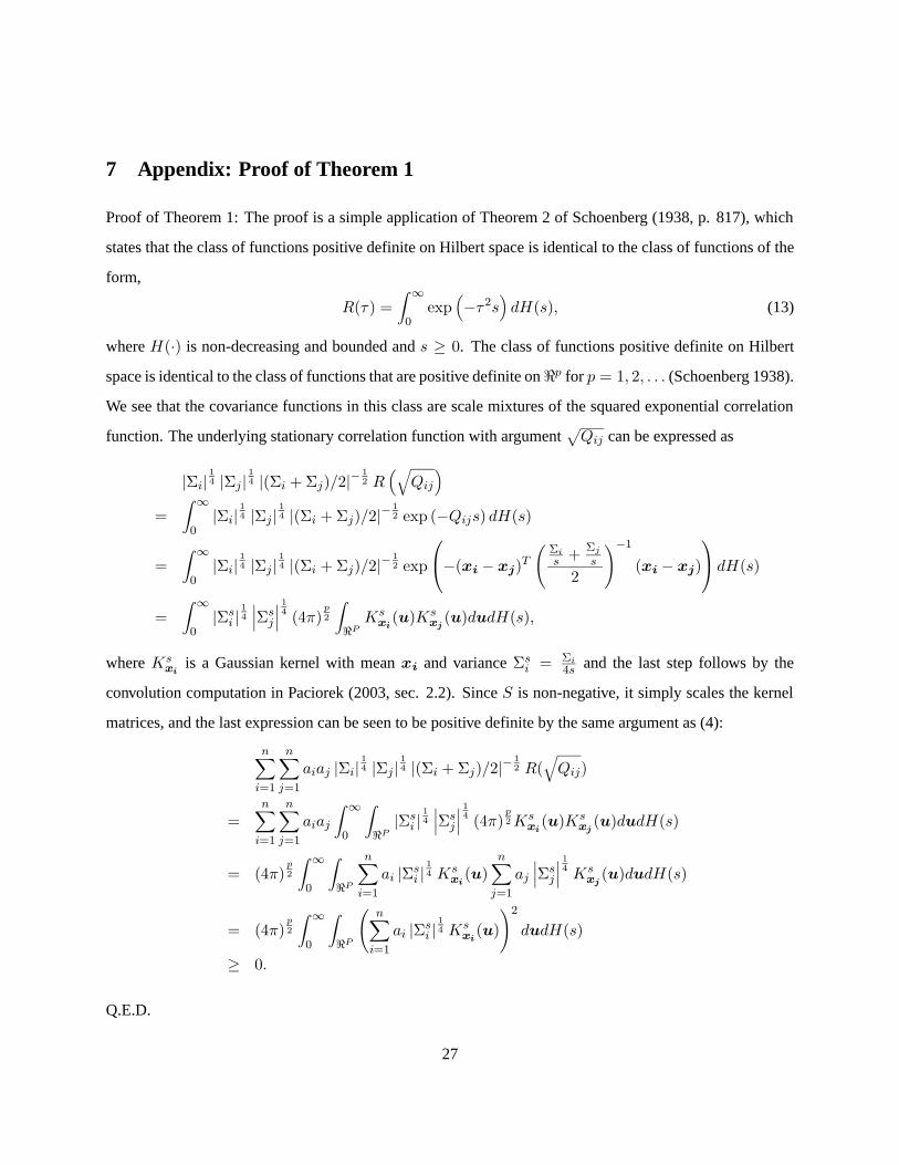
7 Appendix: Proof of Theorem 1

Proof of Theorem 1: The proof is a simple application of Theorem 2 of Schoenberg (1938, p. 817), which

states that the class of functions positive definite on Hilbert space is identical to the class of functions of the

form,

R(τ) =

∫

∞

0exp

(

−τ2s)

dH(s), (13)

where H(·) is non-decreasing and bounded and s ≥ 0. The class of functions positive definite on Hilbert

space is identical to the class of functions that are positive definite on <p for p = 1, 2, . . . (Schoenberg 1938).

We see that the covariance functions in this class are scale mixtures of the squared exponential correlation

function. The underlying stationary correlation function with argument√

Qij can be expressed as

|Σi|1

4 |Σj |1

4 |(Σi + Σj)/2|−1

2 R(√

Qij

)

=

∫

∞

0|Σi|

1

4 |Σj |1

4 |(Σi + Σj)/2|−1

2 exp (−Qijs) dH(s)

=

∫

∞

0|Σi|

1

4 |Σj |1

4 |(Σi + Σj)/2|−1

2 exp

−(xi − xj)T

(

Σi

s +Σj

s

2

)−1

(xi − xj)

dH(s)

=

∫

∞

0|Σs

i |1

4

∣

∣

∣Σsj

∣

∣

∣

1

4 (4π)p

2

∫

<PKs

xi(u)Ks

xj(u)dudH(s),

where Ksxi

is a Gaussian kernel with mean xi and variance Σsi = Σi

4s and the last step follows by the

convolution computation in Paciorek (2003, sec. 2.2). Since S is non-negative, it simply scales the kernel

matrices, and the last expression can be seen to be positive definite by the same argument as (4):

n∑

i=1

n∑

j=1

aiaj |Σi|1

4 |Σj |1

4 |(Σi + Σj)/2|−1

2 R(√

Qij)

=n∑

i=1

n∑

j=1

aiaj

∫

∞

0

∫

<P|Σs

i |1

4

∣

∣

∣Σsj

∣

∣

∣

1

4 (4π)p

2Ksxi

(u)Ksxj

(u)dudH(s)

= (4π)p

2

∫

∞

0

∫

<P

n∑

i=1

ai |Σsi |

1

4 Ksxi

(u)n∑

j=1

aj

∣

∣

∣Σsj

∣

∣

∣

1

4 Ksxj

(u)dudH(s)

= (4π)p

2

∫

∞

0

∫

<P

(

n∑

i=1

ai |Σsi |

1

4 Ksxi

(u)

)2

dudH(s)

≥ 0.

Q.E.D.

27

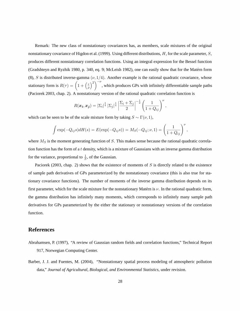
Remark: The new class of nonstationary covariances has, as members, scale mixtures of the original

nonstationary covariance of Higdon et al. (1999). Using different distributions,H , for the scale parameter, S,

produces different nonstationary correlation functions. Using an integral expression for the Bessel function

(Gradshteyn and Ryzhik 1980, p. 340, eq. 9; McLeish 1982), one can easily show that for the Matérn form

(8), S is distributed inverse-gamma (ν, 1/4). Another example is the rational quadratic covariance, whose

stationary form is R(τ) =

(

1 +(

τρ

)2)−ν

, which produces GPs with infinitely differentiable sample paths

(Paciorek 2003, chap. 2). A nonstationary version of the rational quadratic correlation function is

R(xi,xj) = |Σi|1

4 |Σj |1

4

∣

∣

∣

∣

Σi + Σj

2

∣

∣

∣

∣

−1

2

(

1

1 +Qij

)ν

,

which can be seen to be of the scale mixture form by taking S ∼ Γ(ν, 1),

∫

exp(−Qijs)dH(s) = E(exp(−Qijs)) = MS(−Qij ; ν, 1) =

(

1

1 +Qij

)ν

,

where MS is the moment generating function of S. This makes sense because the rational quadratic correla-

tion function has the form of a t density, which is a mixture of Gaussians with an inverse gamma distribution

for the variance, proportional to 1S , of the Gaussian.

Paciorek (2003, chap. 2) shows that the existence of moments of S is directly related to the existence

of sample path derivatives of GPs parameterized by the nonstationary covariance (this is also true for sta-

tionary covariance functions). The number of moments of the inverse gamma distribution depends on its

first parameter, which for the scale mixture for the nonstationary Matérn is ν. In the rational quadratic form,

the gamma distribution has infinitely many moments, which corresponds to infinitely many sample path

derivatives for GPs parameterized by the either the stationary or nonstationary versions of the correlation

function.

References

Abrahamsen, P. (1997), “A review of Gaussian random fields and correlation functions,” Technical Report

917, Norwegian Computing Center.

Barber, J. J. and Fuentes, M. (2004), “Nonstationary spatial process modeling of atmospheric pollution

data,” Journal of Agricultural, Biological, and Environmental Statistics, under revision.

28

Christensen, O., Roberts, G., and Sköld, M. (2003), “Robust MCMC methods for spatial GLMMs,” in

preparation.

Cowles, M. K. and Carlin, B. P. (1996), “Markov chain Monte Carlo convergence diagnostics: A compara-

tive review,” Journal of the American Statistical Association, 91, 883–904.

Crainiceanu, C. M., Ruppert, D., and Carroll, R. J. (2004), “Spatially Adaptive Bayesian P-Splines with

Heteroscedastic Errors,” Technical Report 61, Department of Biotatistics, Johns Hopkins University.

Cressie, N. (1993), Statistics for Spatial Data (Revised ed.): Wiley-Interscience.

Damian, D., Sampson, P., and Guttorp, P. (2001), “Bayesian estimation of semi-parametric non-stationary

spatial covariance structure,” Environmetrics, 12, 161–178.

Denison, D., Mallick, B., and Smith, A. (1998), “Bayesian MARS,” Statistics and Computing, 8, 337–346.

Denison, D. G., Holmes, C. C., Mallick, B. K., and Smith, A. F. M. (2002), Bayesian Methods for Nonlinear

Classification and Regression, New York: Wiley.

DiMatteo, I., Genovese, C., and Kass, R. (2001), “Bayesian curve-fitting with free-knot splines,” Biometrika,

88, 1055–1071.

Friedman, J. (1991), “Multivariate adaptive regression splines,” Annals of Statistics, 19, 1–141.

Fuentes, M. (2001), “A high frequency kriging approach for non-stationary environmental processes,” En-

vironMetrics, 12, 469–483.

Fuentes, M. and Smith, R. (2001), “A New Class of Nonstationary Spatial Models,” Technical report, North

Carolina State University, Department of Statistics.

Gelfand, A., Sahu, S., and Carlin, B. (1996), “Efficient parametrizations for generalized linear mixed

models,” in Bayesian Statistics 5, eds. J. Bernardo, J. Berger, A. Dawid, and A. Smith, pp. 165–180.

Gibbs, M. (1997), Bayesian Gaussian Processes for Classification and Regression, unpublished Ph.D.

dissertation, Univ. of Cambridge.

29

Gradshteyn, I. and Ryzhik, I. (1980), Tables of Integrals, Series and Products: Corrected and Enlarged

Edition, New York: Academic Press, Inc.

Green, P. and Silverman, B. (1994), Nonparametric Regression and Generalized Linear Models, Boca

Raton: Chapman & Hall/CRC.

Haas, T. C. (1995), “Local prediction of a spatio-temporal process with an application to wet sulfate depo-

sition,” Journal of the American Statistical Association, 90, 1189–1199.

Hastie, T. J. and Tibshirani, R. J. (1990), Generalized Additive Models, London: Chapman & Hall Ltd.

Higdon, D. (1998), “A process-convolution approach to modeling temperatures in the North Atlantic

Ocean,” Journal of Environmental and Ecological Statistics, 5, 173–190.

Higdon, D., Swall, J., and Kern, J. (1999), “Non-stationary spatial modeling,” in Bayesian Statistics 6, eds.

J. Bernardo, J. Berger, A. Dawid, and A. Smith, Oxford, U.K.: Oxford University Press, pp. 761–768.

Holmes, C. and Mallick, B. (2001), “Bayesian regression with multivariate linear splines,” Journal of the

Royal Statistical Society, Series B, 63, 3–17.

Hwang, J.-N., Lay, S.-R., Maechler, M., Martin, D., and Schimert, J. (1994), “Regression modeling in back-

propagation and projection pursuit learning,” IEEE Transactions on Neural Networks, 5, 342–353.

Kammann, E. and Wand, M. (2003), “Geoadditive models,” Applied Statistics, 52, 1–18.

Lang, S. and Brezger, A. (2004), “Bayesian p-splines,” Journal of Computational and Graphical Statistics,

13, 183–212.

MacKay, D. and Takeuchi, R. (1995), “Interpolation models with multiple hyperparameters,”.

McLeish, D. (1982), “A robust alternative to the normal distribution,” The Canadian Journal of Statistics,

10, 89–102.

Neal, R. (1993), “Probabilistic Inference Using Markov Chain Monte Carlo Methods,” Technical Report

CRG-TR-93-1, Department of Computer Science, University of Toronto.

30

(1996), Bayesian Learning for Neural Networks, New York: Springer.

Ngo, L. and Wand, M. (2004), “Smoothing with mixed model software,” Journal of Statistical Software, 9.

Paciorek, C. (2003), Nonstationary Gaussian Processes for Regression and Spatial Modelling, unpublished

Ph.D. dissertation, Carnegie Mellon University, Department of Statistics.

Paciorek, C. and Ryan, L. (in prep.), “A Bayesian spectral basis model outperforms other approaches when

fitting binary spatial data,” in prep.

Paciorek, C. and Schervish, M. (2004), “Nonstationary covariance functions for Gaussian process re-

gression,” in Advances in Neural Information Processing Systems 16, eds. S. Thrun, L. Saul, and B.

Schölkopf, Cambridge, MA: MIT Press, pp. 273–280.

Rasmussen, C. E. and Ghahramani, Z. (2002), “Infinite mixtures of Gaussian process experts,” in Advances

in Neural Information Processing Systems 14, eds. T. G. Dietterich, S. Becker, and Z. Ghahramani,

Cambridge, MA: MIT Press.

Sampson, P. and Guttorp, P. (1992), “Nonparametric estimation of nonstationary spatial covariance struc-

ture,” J. Am. Stat. Assoc., 87, 108–119.

Schmidt, A. and O’Hagan, A. (2003), “Bayesian Inference for Nonstationary Spatial Covariance Structures

via Spatial Deformations,” Journal of the Royal Statistical Society, Series B, 65, 743–758.

Schoenberg, I. (1938), “Metric spaces and completely monotone functions,” Ann. of Math., 39, 811–841.

Seeger, M. and Williams, C. (2003), “Fast forward selection to speed up sparse Gaussian process regression,”

in Workshop on AI and Statistics 9.

Smith, R. (2001), “Environmental Statistics,” Technical report, Department of Statistics, University of North

Carolina.

Stein, M. (1999), Interpolation of Spatial Data : Some Theory for Kriging, N.Y.: Springer.

(2005), “Nonstationary spatial covariance functions,” submitted to Statistics and Probability Letters,

in submission.

31

Swall, J. (1999), Non-Stationary Spatial Modeling Using a Process Convolution Approach, unpublished

Ph.D. dissertation, Duke University, Institute of Statistics and Decision Sciences.

Tresp, V. (2001), “Mixtures of Gaussian processes,” in Advances in Neural Information Processing Systems

13, eds. T. K. Leen, T. G. Dietterich, and V. Tresp, MIT Press, pp. 654–660.

Wikle, C. (2002), “Spatial modeling of count data: A case study in modelling breeding bird survey data

on large spatial domains,” in Spatial Cluster Modelling, eds. A. Lawson and D. Denison, Chapman &

Hall, pp. 199–209.

Williams, C., Rasmussen, C., Schwaighofer, A., and Tresp, V. (2002), “Observations on the Nyström

Method for Gaussian Process Prediction,” Technical report, Gatsby Computational Neuroscience Unit,

University College London.

Wood, A. and Chan, G. (1994), “Simulation of stationary Gaussian processes in [0, 1]d,” Journal of Com-

putational and Graphical Statistics, 3, 409–432.

Wood, S., Jiang, W., and Tanner, M. (2002), “Bayesian mixture of splines for spatially adaptive nonpara-

metric regression,” Biometrika, 89, 513–528.

Wood, S. N. (2000), “Modelling and smoothing parameter estimation with multiple quadratic penalties,”

Journal of the Royal Statistical Society, Series B, 62(2), 413–428.

(2003), “Thin plate regression splines,” Journal of the Royal Statistical Society, Series B, 65(1),

95–114.

Zhang, H. (2004), “Inconsistent estimation and asymptotically equal interpolation in model-based geostatis-

tics,” J. Am. Stat. Assoc., 99, 250–261.

32

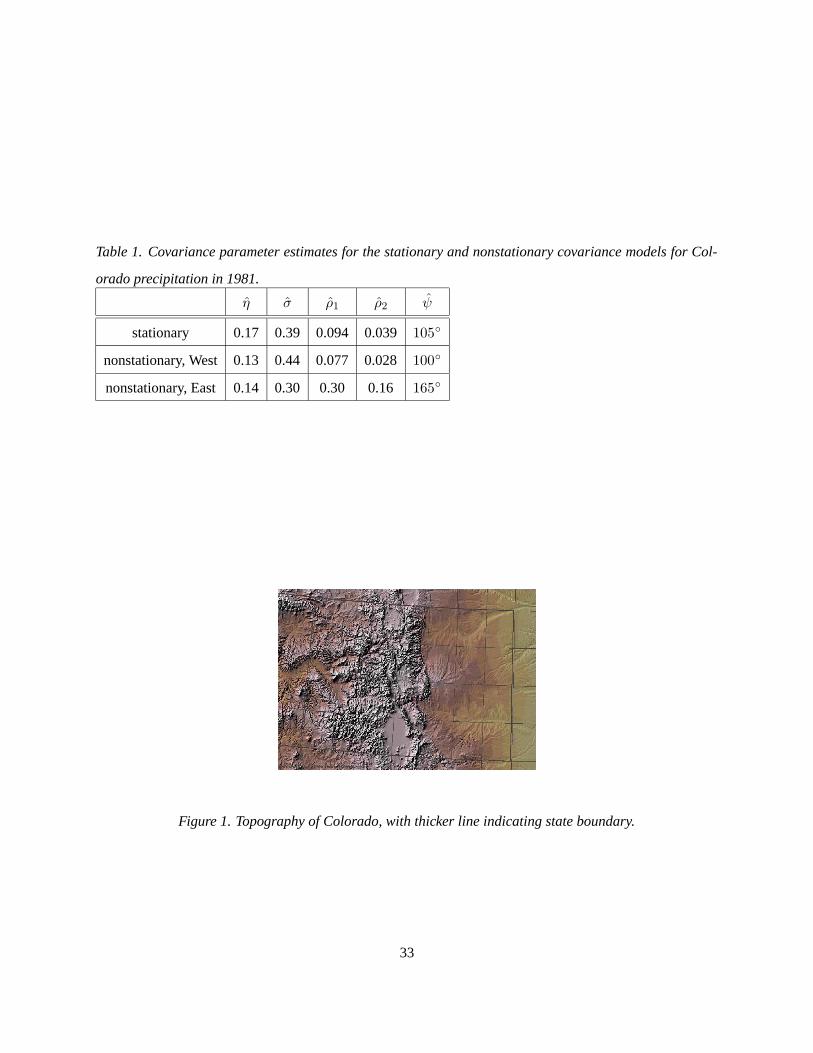
Table 1. Covariance parameter estimates for the stationary and nonstationary covariance models for Col-

orado precipitation in 1981.

η σ ρ1 ρ2 ψ

stationary 0.17 0.39 0.094 0.039 105

nonstationary, West 0.13 0.44 0.077 0.028 100

nonstationary, East 0.14 0.30 0.30 0.16 165

Figure 1. Topography of Colorado, with thicker line indicating state boundary.

33

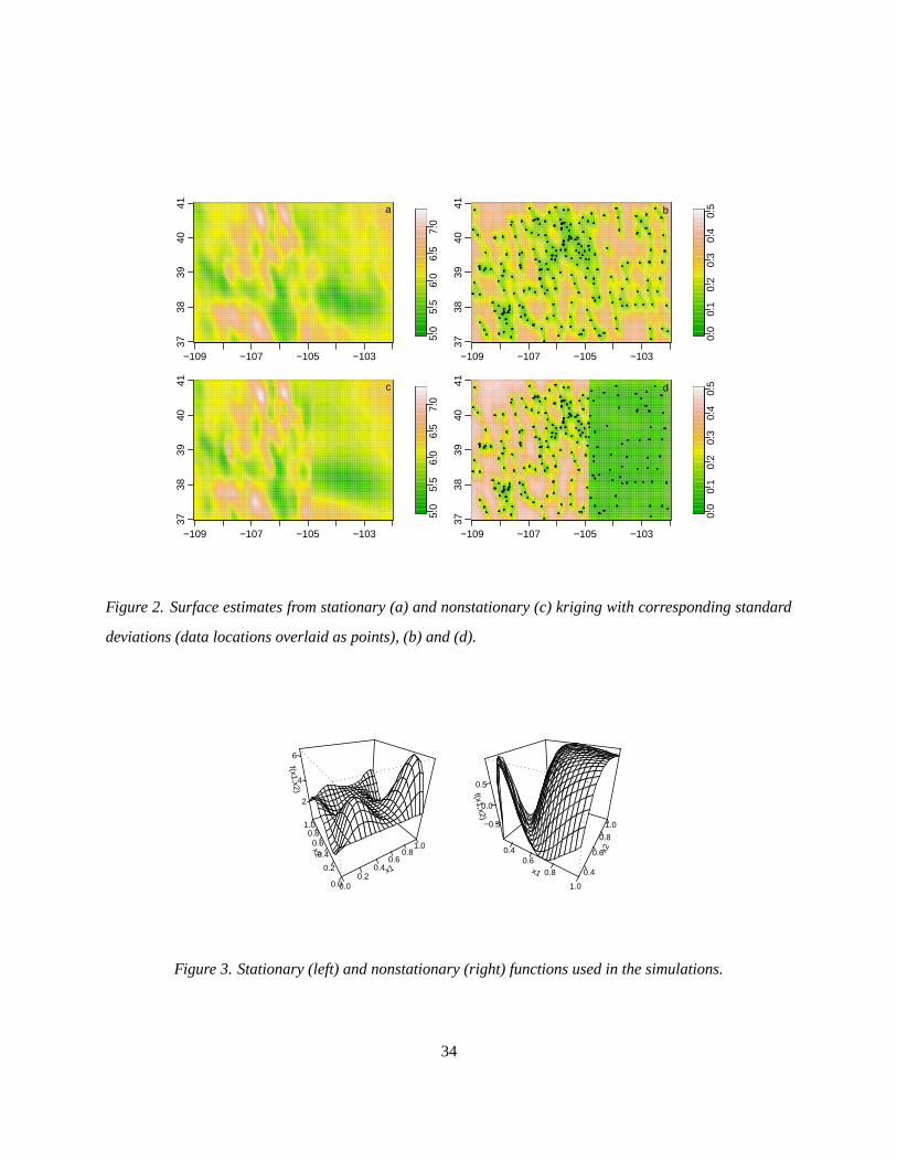
−109 −107 −105 −103

3738

3940

41

5.0

5.5

6.0

6.5

7.0

a

−109 −107 −105 −103

3738

3940

41

0.0

0.1

0.2

0.3

0.4

0.5b

−109 −107 −105 −103

3738

3940

41

5.0

5.5

6.0

6.5

7.0

c

−109 −107 −105 −103

3738

3940

41

0.0

0.1

0.2

0.3

0.4

0.5d

Figure 2. Surface estimates from stationary (a) and nonstationary (c) kriging with corresponding standard

deviations (data locations overlaid as points), (b) and (d).

x1

0.00.2

0.40.6

0.81.0x2

0.0

0.2

0.40.6

0.81.0

f(x1,x2)

2

4

6

x1

0.40.6

0.8

1.0

x2

0.4

0.6

0.8

1.0

f(x1,x2)

−0.5

0.0

0.5

Figure 3. Stationary (left) and nonstationary (right) functions used in the simulations.

34

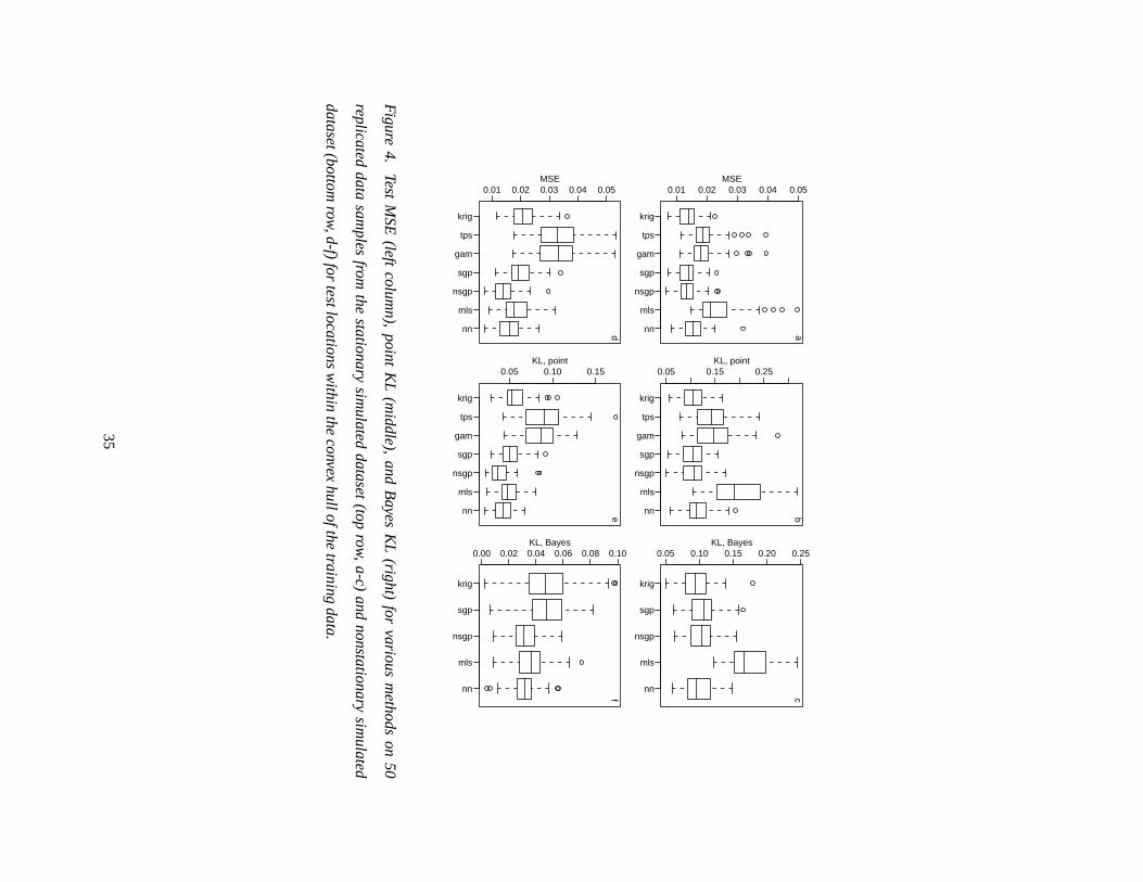
krig

tps

gam

sgp

nsgp

mls

nn

0.01 0.02 0.03 0.04 0.05MSE

a

krig

tps

gam

sgp

nsgp

mls

nn

0.05 0.15 0.25KL, point

b

krig

sgp

nsgp

mls

nn

0.05 0.10 0.15 0.20 0.25KL, Bayes

c

krig

tps

gam

sgp

nsgp

mls

nn

0.01 0.02 0.03 0.04 0.05MSE

d

krig

tps

gam

sgp

nsgp

mls

nn

0.05 0.10 0.15KL, point

e

krig

sgp

nsgp

mls

nn

0.00 0.02 0.04 0.06 0.08 0.10KL, Bayes

f

Figure

4.Test

MSE

(leftcolum

n),point

KL

(middle),

andB

ayesK

L(right)

forvarious

methods

on50

replicateddata

samples

fromthe

stationarysim

ulateddataset

(toprow

,a-c)

andnonstationary

simulated

dataset(bottomrow

,d-f)for

testlocationsw

ithinthe

convexhullofthe

trainingdata.

35

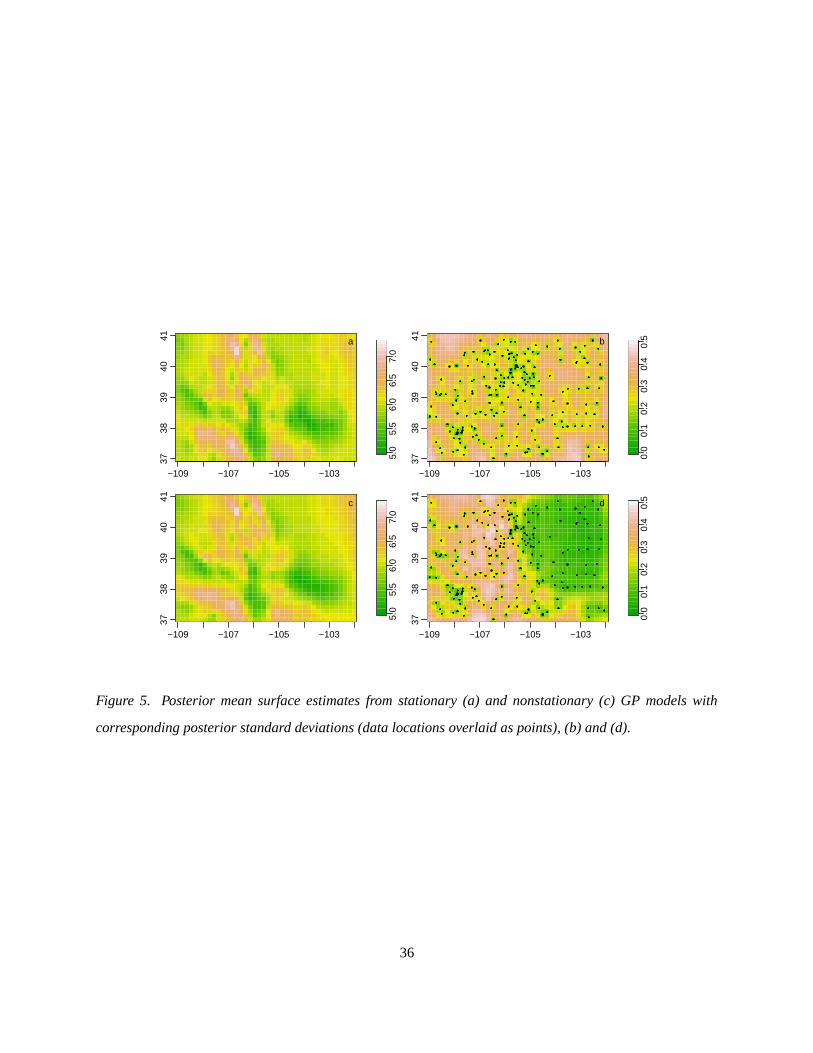
−109 −107 −105 −103

3738

3940

41

5.0

5.5

6.0

6.5

7.0

a

−109 −107 −105 −103

3738

3940

41

0.0

0.1

0.2

0.3

0.4

0.5b

−109 −107 −105 −103

3738

3940

41

5.0

5.5

6.0

6.5

7.0

c

−109 −107 −105 −103

3738

3940

41

0.0

0.1

0.2

0.3

0.4

0.5d

Figure 5. Posterior mean surface estimates from stationary (a) and nonstationary (c) GP models with

corresponding posterior standard deviations (data locations overlaid as points), (b) and (d).

36

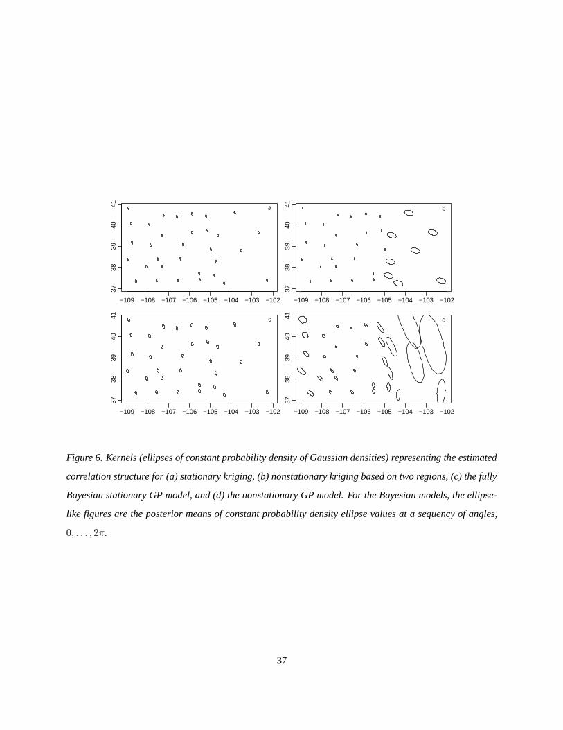
−109 −108 −107 −106 −105 −104 −103 −102

3738

3940

41 a

−109 −108 −107 −106 −105 −104 −103 −102

3738

3940

41 b

−109 −108 −107 −106 −105 −104 −103 −102

3738

3940

41 c

−109 −108 −107 −106 −105 −104 −103 −102

3738

3940

41 d

Figure 6. Kernels (ellipses of constant probability density of Gaussian densities) representing the estimated

correlation structure for (a) stationary kriging, (b) nonstationary kriging based on two regions, (c) the fully

Bayesian stationary GP model, and (d) the nonstationary GP model. For the Bayesian models, the ellipse-

like figures are the posterior means of constant probability density ellipse values at a sequency of angles,

0, . . . , 2π.

37

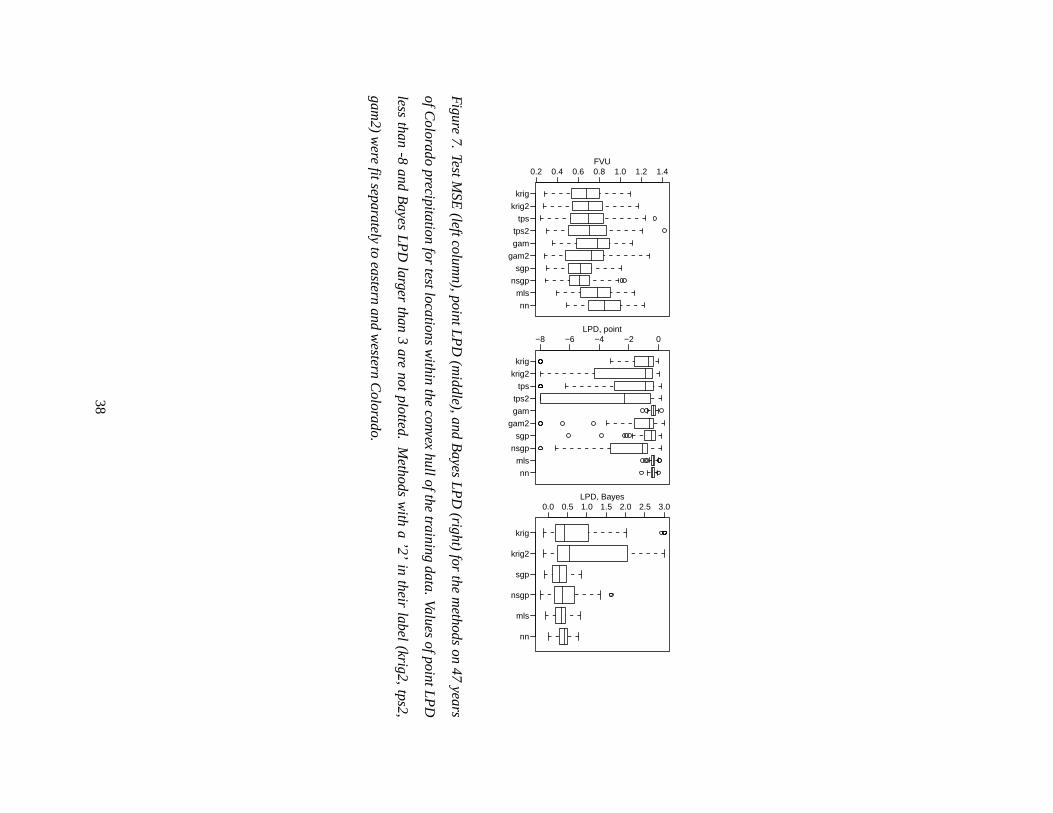
krig

krig2

tps

tps2

gam

gam2

sgp

nsgp

mls

nn

0.2 0.4 0.6 0.8 1.0 1.2 1.4FVU

krig

krig2

tps

tps2

gam

gam2

sgp

nsgp

mls

nn

−8 −6 −4 −2 0LPD, point

krig

krig2

sgp

nsgp

mls

nn

0.0 0.5 1.0 1.5 2.0 2.5 3.0LPD, Bayes

Figure

7.TestM

SE(leftcolum

n),pointLP

D(m

iddle),andB

ayesL

PD

(right)for

them

ethodson

47years

ofColorado

precipitationfor

testlocationsw

ithinthe

convexhullofthe

trainingdata.

ValuesofpointL

PD

lessthan

-8and

Bayes

LP

Dlarger

than3

arenot

plotted.M

ethodsw

itha

’2’in

theirlabel

(krig2,tps2,

gam2)

were

fitseparatelyto

easternand

western

Colorado.

38