S

S

S

S

S

SS

S

S S

S

SS

SS

S

SSS

S

S

S

S

S

S

S

S

S

S

S

S

S

S

S

S

S

S

S

S

S

S

T

TT

T

T

T

T

T

T T

T

TTTT

T

TTT

T

U

U

U

U

U

U U

U

U

U

U

U

U

U

U

U

U U

U

U

U

U

U

U

U

U

U

UU

U

UU

U

U

Ú

Ú

Ú

Ú

Ú

Ú

Ú

Ú

Ú

Ú

Ú

ÚÚ

Ú

Ú

Ú

Ú

Ú

ÚÚ

Ú

Ú

Ú

Ú

Ú

Ú

Ú

Ú

ÚÚ Ú

Ú

Ú

Ú

Ú

Ú

Ú

Ú

Ú Ú

Ú

Ú

Ú

Ú

Ú

ÚÚÚÚÚÚ

Ú

Ú

Ú

Ú

Ú

Ú

Ú

Ú

Ú

Ú

Ú

Ú

Ú

Ú

ÚÚ

Ú

Ú

Ú

Ú

Ú

ÚÚ

Spatial Modelling using the Mahalanobis Statistic:Two Examples from the Discipline of Plant Geography

R. J. DeVries

Ph.D. Student, School of Environmental and Life Sciences, University of Newcastle E-Mail: Robert.Devries@newcastle.edu.au

Keywords: plant geography; habitat modelling; Mahalanobis distance; rainforest, Eucalyptus cannonii.

EXTENDED ABSTRACT

One of the most important practical pursuits in the discipline of plant geography is the production of vegetation community maps. Due to the inherent complexity of most vegetation, this typically requires modelling the distribution of communities in relation to potential predictor variables such as rainfall and temperature. Despite considerable advances in the field of habitat modelling, many of the available techniques remain inaccessible to those working within the discipline, principally due to the steep learning curve required to master them. An exception to this general rule is the ArcView® 3.x extension developed by Jenness (2003) which applies the Mahalanobis statistic (D2), an n-dimensional distance measure which addresses the problem of interaction and covariance between variables.

This paper explores the potential application of D2 to modelling the spatial distribution of plant species and vegetation communities within a geographic information system (GIS). The calculation and characteristics of the D2 statistic are described along with its GIS implementation. Two case studies are presented to illustrate the potential utility of D2 to address the challenge of large spatial datasets; multidimensional, vector-valued data; spatial autocorrelation; and the need to generalise areal properties from limited, presence-only point data.

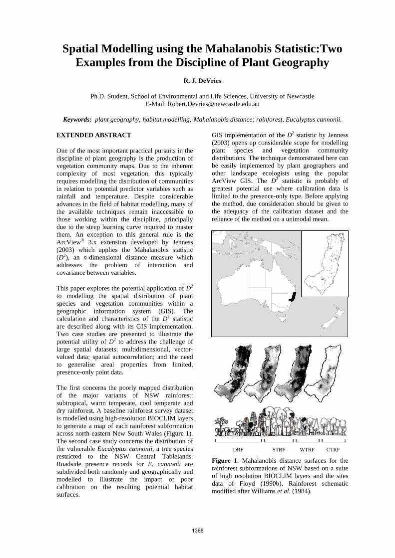
The first concerns the poorly mapped distribution of the major variants of NSW rainforest: subtropical, warm temperate, cool temperate and dry rainforest. A baseline rainforest survey dataset is modelled using high-resolution BIOCLIM layers to generate a map of each rainforest subformation across north-eastern New South Wales (Figure 1). The second case study concerns the distribution of the vulnerable Eucalyptus cannonii, a tree species restricted to the NSW Central Tablelands. Roadside presence records for E. cannonii are subdivided both randomly and geographically and modelled to illustrate the impact of poor calibration on the resulting potential habitat surfaces.

GIS implementation of the D2 statistic by Jenness (2003) opens up considerable scope for modelling plant species and vegetation community distributions. The technique demonstrated here can be easily implemented by plant geographers and other landscape ecologists using the popular ArcView GIS. The D2 statistic is probably of greatest potential use where calibration data is limited to the presence-only type. Before applying the method, due consideration should be given to the adequacy of the calibration dataset and the reliance of the method on a unimodal mean.

DRF STRF WTRF CTRF

Figure 1. Mahalanobis distance surfaces for the rainforest subformations of NSW based on a suite of high resolution BIOCLIM layers and the sites data of Floyd (1990b). Rainforest schematic modified after Williams et al. (1984).

1368

1. INTRODUCTION

One of the most important practical pursuits in the discipline of plant geography is the production of vegetation community maps which increasingly serve as surrogates for biodiversity in regional land use planning processes (Ferrier et al. 2002). Due to the inherent complexity and spatial heterogeneity of most vegetation, and the typical mismatch between the large area required to be mapped and the small area subject to detailed field survey; the production of a vegetation map is more a process of spatial modelling than an exercise in cartography (Cawsey et al. 2002).

The purpose of this paper is to describe and demonstrate a simple but powerful spatial modelling technique that may suite plant geographers and other non-specialists who are similarly struggling with large spatial datasets; multidimensional, vector-valued data; spatial autocorrelation; and the need to generalize areal properties from limited point data. Specifically, this paper introduces the Mahalanobis distance statistic (D2), discusses its implementation in a GIS and spatial modelling context, and demonstrates its application to two quite district practical vegetation mapping problems. The first concerns the poorly mapped distribution of the major variants of NSW rainforest: subtropical, warm temperate, cool temperate and dry rainforest. The second concerns the distribution of the vulnerable Eucalyptus cannonii, a tree species restricted to the NSW Central Tablelands. The former case study serves to illustrate how limited survey data can be used in combination with abiotic predictor variables to produce meaningful vegetation maps. The latter illustrates the impact of poor model calibration and, conversely, the benefit of sampling across the full environmental range of a species.

2. PREDICTIVE HABITAT MODELLING

The challenge of modelling the spatial distribution of plant species or vegetation communities is considerable, not only as a consequence of the nature of vegetation but because of the many problems of drawing inferences about ecological processes from geographic patterns (Keitt et al. 2002). Guisan and Zimmermann (2000) provide an excellent review of the many potential approaches to predictive habitat modelling (e.g. environmental envelopes, generalised linear / additive regression, classification trees, environmental ordination, neural networks). Unfortunately, many of these techniques remain inaccessible to those working within the discipline of plant geography, principally due to the steep learning curve required

to master them. In contrast, the ArcView 3.x modelling extension developed by Jenness (2003), which applies the (D2) statistic, can be implemented in minutes.

3. MAHALANOBIS DISTANCE

D2 is a dimensionless measure of the distance between each observation in a multidimensional point cloud and the centroid of that cloud (Mahalanobis 1936, Thatcher et al. 2003). In the context of habitat modelling, equal distances imply equal likelihoods or similarities to the multivariate mean habitat (Roberts 2000). The calculation of the statistic begins with the derivation of a variance-covariance matrix. D2 can then be calculated for any given observation, or in the case of GIS analysis, for any given raster cell according to the formula:

(1) D2 = (x - m)T C-1 (x - m)

where: D2 = Mahalanobis distance X = vector of data m = vector of mean values of independent variables C-1 = inverse covariance matrix of independent variables T = indicates that the vector should be transposed

The end result of these calculations is measure of the distance of a given observation from the mean of all observation in multidimensional space. Those involved in landscape analysis may prefer to regard D2 as a measure of “landscape similarity”, relative to a set of sample sites. As an n-dimensional distance measure, D2 has several advantages over the various forms of the Minkowski distance, specifically, it is not distorted by the different metrics of the individual coordinates or any correlations between variables (Lohninger 1999). D2 is dimensionless but its values can be converted into Chi-Square probabilities where the ‘predictor’ variables are normally distributed.

The Mahalanobis statistic has been implemented in a GIS context by Jenness Enterprises (Jenness 2003) as a very user-friendly and well documented ArcView extension, “mahalanobis.avx”. The extension, which is free to download at www.jennessent.com/arcview/mahalanobis.htm, requires ArcView 3.x and the Spatial Analyst extension. The mahalanobis.avx extension is limited to a maximum of 8 predictor grids due to a limitation in the Spatial Analyst extension. All D2 surfaces presented in this paper were generated using the mahalanobis.avx extension and raw D2 values.

1369

4. CASE STUDY NO.1 – MAPPING RAINFOREST SUBFORMATIONS

In Australia, rainforest vegetation is scattered across the continent’s full latitudinal range, from the tropics to Tasmania, as a green archipelago in a vast sea of fire-prone, eucalypt-dominated vegetation (Herbert 1967, Bowman 2000). The State of NSW straddles roughly one quarter of this latitudinal range, incorporating the subtropical, dry, warm temperate and cool temperate rainforest subformations (Floyd 1989, Adam 1992). George Baur, one of the State’s pioneering forest ecologists, explains that: “The types would not all be classed as “rainforest” in any comprehensive worldwide classification of vegetation, but all show close affinities with undoubted rainforest communities and their features are such as to set them apart as a very distinctive and well-marked group. Four leagues are recognised within the group, these being distinguished primarily on the structure of the communities, though species composition tends to parallel this structural classification rather closely.” (Forestry Commission of NSW 1989:30).

The four main rainforest subformations predominantly occupy ‘refugial’ or fire-protected positions within the landscape and segregate according to temperature and available moisture such that warm and wet areas support subtropical rainforest; warm and dry areas support dry rainforest; cool and wet areas support warm temperate rainforest; and cold and wet areas support cool temperate rainforest (Williams et al. 1984, Floyd 1989, 1990a&b; Figure 1). The segregation of subtropical and warm temperate rainforest is complicated by an interaction with soil fertility, such that former is found at higher elevations on fertile soils whilst the latter is found at lower elevations on infertile soils.

At present, there is no readily available, high resolution data layer delineating the present extent of NSW rainforest vegetation. Even where local vegetation map datasets are available, floristic variation within rainforest is not typically mapped, not even to the subformation level. An exception to this is the dated Forest Type mapping which is limited to State Forest tenure (Forestry Commission of NSW 1989). Ongoing research by the author seeks to integrate available floristic and spatial information on the rainforests of NSW to yield a spatial data baseline for the conservation of rainforest plant communities.

As a first step towards this goal, the ‘representatives stands’ sites data of A. G. Floyd (1990b), which supports the classification of the

State’s rainforest into 13 rainforest plant alliances and 57 suballiances, was imported into ArcView and the 220 sites were separated by subformation so that each subformation had its own sites layer. The following 25 metre resolution BIOCLIM layers (Houlder et al. 001) were selected as potential predictors: annual mean temperature; mean temperature of the coldest quarter; annual precipitation; precipitation of the driest quarter; annual mean radiation; and radiation of the driest quarter. All model inputs were clipped to a study area including all of the major coastal catchments north from the Hunter River (Figure 1), thereby encompassing the biologically diverse north-east region. This 8.5 million hectare study area encompasses perhaps 90% of the State’s rainforest (Floyd 1990a).

Mahalanobis surfaces were derived from each subformation sites layer using the aforementioned suite of BIOCLIM layers (Figure 1). These surfaces were then integrated into a single coverage using a series of logical operations in the ArcView map calculator to allocate grid cells to the subformation with the lowest Mahalanobis distance. The resulting map is presented in Figure 2 which includes an inset of the Barrington Tops district to illustrate that for mapping purposes the layer can be clipped to the present mapped extent of rainforest vegetation (a tiny fraction of the study area).

Detailed evaluation of this spatial model must await the integration of other vegetation map and flora survey datasets but, overall, it appears to match expectations based on the landmark descriptive/qualitative work of Floyd (1990a&b), albeit with the probable misclassification of large areas of subtropical and warm temperate rainforest due the absence of soil fertility as a predictor variable. Perhaps the most striking pattern in the subformation map is the very limited extent of cool temperate rainforest (just 2.3% of the study area).

The cool temperate rainforest model was recently used in a successful search for Nothofagus moorei (Antarctic Beech) in the extensive Banda Banda region (Figure 3). The mean D2 value of the 26 recorded sites was 3.88. A single site was not well accounted for by the model (D2=21), presumably because of its low altitude (903m compared to a mean of 1054m), the lowest of all sites. This observation points to another advantage of the Mahalanobis technique, namely, its ability to rapidly identify outliers.

1370

S

S

S

S

S

SS

S

S S

S

SS

SS

S

SSS

S

S

S

S

S

S

S

S

S

S

S

S

S

S

S

S

S

S

S

S

S

S

T

TT

T

T

T

T

T

T T

T

TTTT

T

TTT

T

U

U

U

U

U

U U

U

U

U

U

U

U

U

U

U

U U

U

U

U

U

U

U

U

U

U

UU

U

UU

U

U

Ú

Ú

Ú

Ú

Ú

Ú

Ú

Ú

Ú

Ú

Ú

ÚÚ

Ú

Ú

Ú

Ú

Ú

ÚÚ

Ú

Ú

Ú

Ú

Ú

Ú

Ú

Ú

ÚÚ Ú

Ú

Ú

Ú

Ú

Ú

Ú

Ú

Ú Ú

Ú

Ú

Ú

Ú

Ú

ÚÚÚÚÚÚ

Ú

Ú

Ú

Ú

Ú

Ú

Ú

Ú

Ú

Ú

Ú

Ú

Ú

Ú

ÚÚ

Ú

Ú

Ú

Ú

Ú

ÚÚ

Hybrid

Subtropical

Dry

Warm Temperate

Cool Temperate

Figure 2. Potential habitat map of rainforest subformations in north-eastern NSW generated by combining individual Mahalanobis subformation surfaces derived from a suite of BIOCLIM predictor layers and the sites data of Floyd (1990b). The inset shows the result of clipping the layer to the mapped extent of rainforest vegetation in the Barrington Tops district (NSW National Parks and Wildlife Service 1998).

Figure 3. Digital elevation model showing the potential distribution of Nothofagus cool temperate rainforest in the Banda Banda region (green) with Nothofagus moorei sites (red cones) located during preliminary validation surveys.

5. CASE STUDY NO.2 - EUCALYPTUS CANNONII

Eucalyptus cannonii is a stringybark to 15 metres high with pendulous branches, similar in many respects to E. macrorhyncha to which it is closely related. Whilst the distinction between the two species is not always obvious in the field (as the taxa tend to intergrade), in most cases E. cannonii can be recognised by its rimmed, often turbinate fruit and rimmed, fusiform buds (Brooker and Kleinig 1999). E. cannonii is listed as vulnerable under the NSW Threatened Species Conservation Act 1995 and the Commonwealth Endangered Species Protection Act 1992 (NSW National Parks and Wildlife Service 2000).

According to the Flora of New South Wales (K. D. Hill in Harden 1991:125), E. cannonii is “Locally frequent but restricted, in sclerophyll woodland on shallow soil on rises; Rylstone to upper Wolgan Valley” on the Central Tablelands and Central Western Slopes. However, Hunter and White (1999:391) state that: “There appears to be no predictable habitat preferences for Eucalyptus cannonii. Evidence indicates wide tolerance of different conditions, with parent rock including: sandstone, shale, basalt, trachyte, claystone, and coarse conglomerates. Often this taxon is found higher on mountains and ridgetops with rocky soils such as talus slopes, cliffs, summits and spires, but it also occurs lower within valleys and on low undulating hills.” A species profile produced by the NSW National Parks and Wildlife Service (2000) indicates that the distribution of the species is somewhat broader than described in the Flora, extending east from Bathurst and Mudgee to Wollemi National Park.

1371

Detailed survey of the roadside distribution of E. cannonii within the Rylstone Shire (in the centre of its range) was undertaken by DeVries and McCauley (2001). This location data, which forms the basis of the following modelling exercise, was acquired using a 12-channel GPS with an averaging function to achieve a horizontal accuracy of typically better than +/-20 m and no worse than +/-50 m (Figure 4). It should be emphasised that the purpose of the modelling was not to elucidate aspects of the ecology of the species or to delineate areas for further targetted surveys, but to evaluate the impact of different model calibration scenarios on Mahalanobis ‘predictions’.

As in the first case study, high resolution BIOCLIM layers were used as the predictor variables, specifically: annual mean temperature; mean temperature of the driest quarter; annual precipitation; precipitation of the driest quarter; annual mean radiation; and radiation of the driest quarter. Five Mahalanobis surfaces were generated using: (A) all presence sites (N=213); (B) a random selection of presence sites (N=109); (C) sites not selected in B (N=104). (D) only the northern sites (N=109); and (E) only the southern sites (N=104). Each Mahalanobis surface is presented in Figure 4.

The surfaces generated using scenarios A, B and C are very similar, suggesting that a random subset of only about half of the total available sites was sufficient to ‘capture’ the main pattern present in the complete dataset. In contrast, the surfaces generated using scenarios D and E (the northern and southern subsets) indicate that where calibration sites do not adequately represent the true environmental range of the species, Mahalanobis surfaces will similarly not reliably represent the potential geographic envelope of the species. This point can also be made numerically, by using Mahalanobis surfaces based on each site subset to predict the occurrence of E. cannonii at sites that are not a member of that subset. The predictive power of each surface can be evaluated by taking the mean distance for the validation sites. Low predicted distances would be expected for E. cannonii where the surface has some predictive power. The relevant data are presented in Figure 4. As this figure demonstrates, surfaces based on the northern and southern sites predict the occurrence of validation sites at a high mean distance (279.07 and 102.74 respectively), meaning that they have little predictive value. In contrast, the surfaces based on the random sites subset predict the occurrence of their validation sites at a low mean distance (7.22 and 5.42 for B and C respectively).

0 50 100 150 200 250 30

E

D

C

B

A

# ###### ### #####

## #

#

#

##

#

#

#

###

#

# #

#

#

#

###

#####

#

#

###### #

###

##

##

#

##############

###

##

#########

###

##

#

###

#

#

## ### ##

### ###### #

#

###

##

######

#######

###

#

#

#

#

#

#

#

# ####

#

#

###

# #### ##

####### #### ###

#

##

###

##

##

## ##

######

##

###

#

######

####

##

Northern and southern sites subsets

A D

B E

Mahalanobis distance

C Mean distances for validation sites

Figure 4. Mahalanobis distance surfaces for Eucalyptus cannonii in the Rylstone district under five model calibration scenarios: (A) all presence sites; (B) a random selection of presence sites; (C) sites not selected in B; (D) only the northern sites; and (E) only the southern sites. The table shows the mean D2 values for all sites (A) and for sites not included in the calibration dataset for scenarios B, C, D and E.

1372

6. DISCUSSION

GIS implementation of the Mahalanobis distance statistic by Jenness (2003) opens up considerable scope for modelling plant species and vegetation community distributions. The technique demonstrated here can be easily implemented by plant geographers and other landscape ecologists using the popular ArcView GIS. The D2 statistic is probably of greatest potential use where calibration data is limited to the presence-only type. Before applying the method, due consideration should be given to the adequacy of the calibration dataset and the reliance of the method on a unimodal mean.

The apparent success of the Mahalanobis technique in describing the distribution of rainforest subformations in NSW may be due, firstly, to the broad environmental and geographic range of the sites sampled by Floyd (1990b) and, secondly, to the use of predictor variables that closely reflect known limits to their environmental distribution. Detailed evaluation of this spatial model must however await the integration of other vegetation map and flora survey datasets.

As the Eucalyptus cannonii case study demonstrates, D2 is a conservative distance statistic and its predictive ability is limited by the adequacy of the calibration dataset. But as Knick and Rotenberry (1998:320) state, “…the Mahalanobis distance technique is not unique in this respect, because all statistical techniques share this classification problem when confronted with configurations outside the original sampling distribution.”

It should also be understood that D2 distances are calculated relative to observed habitat use and cannot be expected to decrease (as if by magic) where new habitat configurations are imposed for the purposes of modelling the impact of habitat change (see Knick and Rotenberry 1998).

Use of D2 for habitat modelling implicitly assumes that all variables used to calculate distances are actually relevant to the biological entity under consideration. Those looking for ecological cause and effect should be advised that D2 distances say nothing about causation, only about the (dis)similarity of parts of the landscape to the multivariate mean habitat. This is not to say that use of the D2 statistic is of no value to ecologists. On the contrary, where the model inputs are carefully chosen to reflect a particular hypothesis of habitat selection, the D2 statistic can be used to map habitat relationships otherwise hidden in the multivariate dataset. At the very least, these maps can be used to better target biological surveys.

7. CONCLUSIONS

The Mahalanobis distance statistic can readily address some of the fundamental challenges of plant geographic research. These challenges include: large spatial datasets; multidimensional, vector-valued data; spatial autocorrelation; and point-to-area generalisation. Of course, where the calibration dataset does not adequately sample the geographic envelope of the modelled subject, or the reliance on a unimodal mean is invalid, outputs will have limited predictive power.

GIS implementation of the D2 statistic by Jenness (2003) constitutes an important practical tool for landscape ecologists. It is hoped that other spatial modelling techniques will be made available to the large ArcView user community, many of whom are actively involved in biodiversity conservation.

Rotenberry et al. (2002) propose a refinement to the classic Mahalanobis approach, involving the decomposition of D2 into its principle vectors, which may identify the variables of greatest relevance to the modelled subject.

8. ACKNOWLEDGMENTS

This research was undertaken as part of ongoing research towards a Ph.D. at the School of Environmental and Life Sciences, University of Newcastle, Australia. I would like to acknowledge the work of Jenness Enterprises for bringing valuable and easy to use GIS-analytic functions into the public domain and the assistance of the NSW Department of Environment and Conservation for providing access to digital rainforest mapping and the BIOCLIM layers. I would also like to thank my supervisor, Stuart Pearson, for his comments on earlier drafts of this paper. Thanks also to Steven Knick and John Rotenberry for assisting with access to several key papers. Of course, this work could not have been undertaken without the financial support of my patron, Angela McCauley.

9. REFERENCES

Bowman, D.M.J.S. (2000), Australian rainforests: islands of green in a land of fire, Cambridge University Press, Cambridge, UK.

Brooker, M.I.H. and D.A. Kleinig (1999), Field guide to eucalypts. Volume 1, South-eastern Australia, second edition, Bloomings Books, Hawthorn, Vic.

Cawsey, E.M., M.P. Austin, and B.L. Baker (2002), Regional vegetation mapping in Australia: a case study in the practical use of

1373

statistical modelling, Biodiversity and Conservation 11: 2239–2274.

DeVries, R.J. and A.C. McCauley (2001), Roadside vegetation in the Rylstone Shire, NSW Central Tablelands and Central Western Slopes: Part 5 – Eucalyptus cannonii, a consultancy report prepared for the Rylstone District Environment Society Inc. by Symbiosis Environmental Consulting Services, Bathurst.

Eastman, J.R. (2003), IDRISI Kilimanjaro: Guide to GIS and Image Processing, Idrisi Manual Version 14.00, Clark Labs, Clark University, Worcester, MA, USA.

Ferrier, S., M. Drielsma, G. Manion, and G. Watson (2002), Extended statistical approaches to modelling spatial pattern in biodiversity in northeast New South Wales. II. Community-level modelling, Biodiversity and Conservation 11: 2309–2338.

Floyd, A.G. (1989), Rainforest trees of mainland south-eastern Australia, Forestry Commission of New South Wales / Inkata Press, Sydney, NSW.

Floyd, A.G. (1990a), Australian Rainforests in New South Wales - Volume I, NSW National Parks and Wildlife Service / Surrey Beatty & Sons Pty. Ltd., Chipping Norton, NSW.

Floyd, A.G. (1990b), Australian rainforests in New South Wales - Volume II, NSW National Parks and Wildlife Service / Surrey Beatty & Sons Pty. Ltd., Chipping Norton, NSW.

Forestry Commission of New South Wales (1989), Research Note 17: Forest Types in New South Wales, Forestry Commission, Sydney.

Guisan, A. and N. E. Zimmermann (2000). Predictive habitat distribution models in ecology, Ecological Modelling 135: 147–186.

Harden, G.J. (1991), Flora of New South Wales - Volume 2, New South Wales University Press, Kensington, NSW.

Herbert, D.A. (1967), Ecological segregation and Australian phytogeographic elements, Proceedings of the Royal Society of Queensland, 78: 110-111.

Houlder, D., M. Hutchinson, H. Nix, and J. McMahon (2001), ANUCLIM 5.1 User’s Guide, Australian National University, Centre for Resource and Environmental Studies, Canberra.

Hunter, J.T. and M. White (1999), Notes on the distribution and conservation status of

Eucalyptus cannonii R.T. Baker, Cunninghamia 6(2): 389-394.

Jenness, J. (2003), Mahalanobis distances (mahalanobis.avx) extension for ArcView 3.x, Jenness Enterprises, Flagstaff, AZ, USA, www.jennessent.com/arcview/mahalanobis.htm.

Keitt, T.H., O.N. Bjørnstad, P.M. Dixon, and S. Citron-Pousty (2002), Accounting for spatial pattern when modeling organism-environment interactions, Ecography 25: 616–625.

Knick, S.T. and J.T. Rotenberry (1998), Limitations to mapping habitat use areas in changing landscapes using the Mahalanobis distance statistic, Journal of Agricultural, Biological, and Environmental Statistics 3(3): 311-322.

Lohninger, H. (1999), Teach/Me Data Analysis (online text-only light edition), Springer-Verlag, Berlin-New York-Tokyo.

Mahalanobis, P.C. (1936), On the generalized distance in statistics, Proceedings National Institute of Science, India, 12: 49-55.

NSW National Parks and Wildlife Service (1998), CRAFTI UNE and LNE Report. A report undertaken as part of the NSW Comprehensive Regional Assessments. Resource and Conservation Planning Division, Planning NSW, Sydney.

NSW National Parks and Wildlife Service (2000), Threatened species information: Eucalyptus cannonii R. Baker, NSW NPWS, Hurstville NSW.

Roberts, A. (2002), Habitat modeling literature review, A report prepared for Don Morgan, Ministry of Forests, Smithers, BC, April 2002.

Rotenberry, J.T., S.T. Knick, and J. Dunn (2002), A minimalist approach to mapping species’ habitat: Pearson’s planes of closest fit. Chapter 22 in Scott, J.M. (ed.), Predicting species occurrences: issues of accuracy and scale, Island Press, Washington DC.

Thatcher, C., F.T. van Manen, and J.D. Clark (2003), Habitat assessment to identify potential sites for Florida Panther reintroduction in the southeast, Final report submitted to the U.S. Fish and Wildlife Service, 24 November 2003.

Williams, J.B., G.J. Harden, and W.J.F. McDonald, (1984), Trees and shrubs in rainforests of New South Wales and southern Queensland, Department of Botany, University of New England, Armidale.

1374