Embed Size (px)
Citation preview

European Scientific Journal June edition vol. 8, No.14 ISSN: 1857 – 7881 (Print) e - ISSN 1857- 7431
79
SPATIAL PREDICTION OF HEAVY METAL POLLUTION
FOR SOILS IN COIMBATORE, INDIA BASED ON ANN AND
KRIGING MODEL
A. Gandhimathi
Associate Professor, Department of Civil Engineering, Kumaraguru College of Technology,
Coimbatore, Tamil Nadu, India
T. Meenambal
Professor, Department of Civil Engineering, Government College of Technology,
Coimbatore, Tamil Nadu, India
Abstract
The concentration of five soil heavy metals (Cr, Pb, and As) was measured in 121 sampling
sites in Coimbatore, Tamil Nadu, India regions known as centres of pollution due to the
chemical and metallurgical activities. The soil samples were collected from locations where
the ground is not sliding and the probability of alluvial deposits is small. The concentration of
heavy metals was measured by using Atomic Absorption spectrometer. Kriging and ANN
techniques were used to develop the model to predict the constituents of the heavy metal in
the soils. In some locations, the concentration for the investigated heavy metals exceeds the
concentration admitted by the guideline. The highest concentration of lead (8.9 ppm) was
found in Ukkadam Lake. The highest concentration of chromium was found in Ganapathi
(3.6 ppm). The highest concentration of Arsenic (5.4 ppm) was found in Sidco Industrial
Estate. The maximum admitted concentrations in the sensitive areas revealed to be exceed
from five to twenty times.
Keywords: Kriging, ANN, Soil Pollution, Heavy metals (Cr, Pb, and As), Coimbatore

European Scientific Journal June edition vol. 8, No.14 ISSN: 1857 – 7881 (Print) e - ISSN 1857- 7431
80
1. Introduction
Heavy metal contamination of soil results mainly due to as mining [1], smelting
procedures [2] and agriculture [3] as well as natural activities. Chemical and metallurgical
industries are the most important sources of heavy metal contamination in the environment
[4]. There are so many metal-based industries located in Coimbatore in an unorganized
manner and is the second largest industrial centre in Tamil Nadu, India. The major industries
include textile, dyeing, electroplating, motor and pump set, foundry and metal casting
industries. According to the present situation, about 4500 textiles, 1200 electroplating
industries, 300 dyeing units and 100 foundries are present in and around Coimbatore.
The metals are classified as ―heavy metals‖ if they have a specific gravity of more
than 5 g/cm3. There are more than sixty heavy metals. Heavy metals get accumulated in soils
and plants causing negative influence on photosynthesis, gaseous exchange, and nutrient
absorption of plants resulting reductions in plant growth, dry matter accumulation and yield
[5, 6]. In small concentrations, the traces of the heavy metals in plants or animals are not
toxic [7]. Lead, cadmium and mercury are exceptions; they are toxic even in very low
concentrations [8].
The main goal of the present research was to assess the heavy metals distribution in
some Coimbatore areas, known as chemical or metallurgy industry centres.
2. Study Area
The study area (Figure-1) is located in the southern part in the state of Tamil Nadu,
India

European Scientific Journal June edition vol. 8, No.14 ISSN: 1857 – 7881 (Print) e - ISSN 1857- 7431
81
Figure-1-Location map of study area
121 locations were selected in the study area to collect the soil samples for analysis.
To avoid contamination of the sample was thoroughly clean, black polythene bag was used in
the collection of soil samples. To clean black polythene bags were dried at lower temperature.
The soil samples were collected at random by digging the soil to about 1 meter at the specific
refuse dumps.
3. Material and methods
The collected soil samples were air-dried and sieved into coarse and fine fractions.
Well-mixed samples of 2 g each were taken in 250 ml glass beakers and digested with 8 ml of
aqua regia on a sand bath for 2 hours. After evaporation to near dryness, the samples were
dissolved with 10 mL of 2% nitric acid, filtered and then diluted to 50 mL with distilled
water.
Heavy metal concentrations of each fraction were analyzed by Atomic Absorption
Spectro photometry. Atomization and Quality assurance was guaranteed through double
determinations and use of blanks for correction of background and other sources of error.
The GLOBEC Kriging Software Package – EasyKrig3.0 was used for creating the
prediction model [9]. The prediction models are depicted in Fig. 2 to 4. The soils with
potential risk of heavy metal pollution were located in isolated spots mainly in the northern
part of the study region.
An artificial Neural Network technique is used to develop a model to predict the
constituents of the heavy metal in the soils [10] such as lead, chromium, arsenic. The
developed neural network model consist of 2 input neurons for latitude and longitude, 6
hidden layers consisting of 10 to 20 neurons in each layer for training the data and 1 neuron
to predict the constituents of the heavy metal in the soils. The architecture of the model is
depicted in Fig. 5 to 7.

European Scientific Journal June edition vol. 8, No.14 ISSN: 1857 – 7881 (Print) e - ISSN 1857- 7431
82
4. Result and discussion
4.1 Kriging Model
The heavy metal from various localities including wetland soil sample were collected,
analyzed and the results were reported. The metals analyzed were Cr, Pb and As. Lead Pb
concentration varies from 0 to 8.9 ppm with a maximum 8.9 ppm at Ukkadam Lake. Reason
for maximum Pb at Ukkadam Lake is due to discharging of sewage water into lake. Cr
concentration ranged between 0 - 3.6 ppm. Maximum concentration was in Ganapathy
because of the concentration of foundry industry. As ranged between 0 – 5.4 Maximum at
Sidco Industrial Estate and Singanallur because of the concentration of electroplating
industry. It is observed that maximum heavy metal pollution near the industrial, traffic
junction and the legendary 'go-slow' of automobiles is the order of the day and in localities of
large population concentration and relatively small areas under poor conditions of sanitation.
Kriging model was used to predict the heavy metal at the unknown point. From the
model of heavy metals we can conclude that the residential areas are uncontaminated with Cr
and moderately contaminated with Pb. Heavy metal accumulation in few prominent wetlands
of 10 localities was analyzed. Pb is maximum in Velangulam Lake Ukkadam, and at the
Sungam Lake.
4.2 ANN Model
The feed forward three layered back propagation network architecture is used to
develop ANN model. The input layer consist of two nodes which represents latitude and
longitude which used to predict the response and the output layer consist of one node which
represents the constituents of the heavy metal in the soils such as lead, chromium, arsenic.
The number of hidden layer and neurons in the hidden layer has been determined by training
several networks.
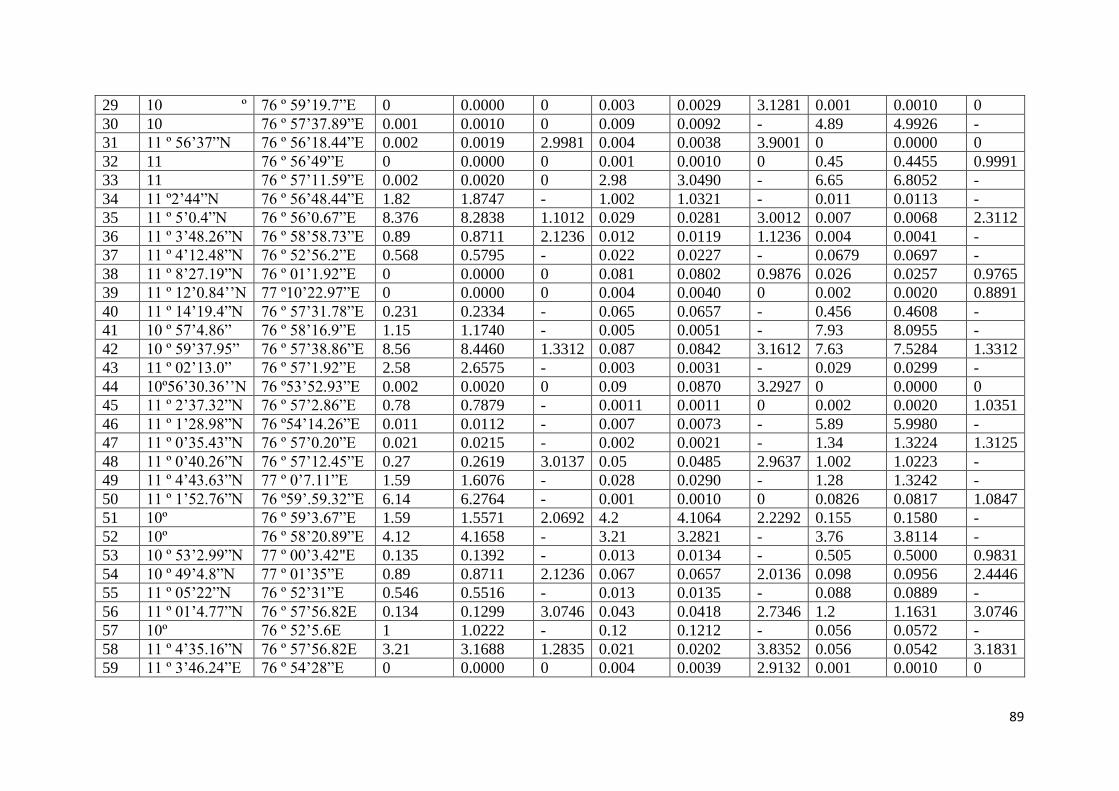
The surveyed, predicted and error percentage of heavy metal is tabulated in table1.
4.3 Comparison of Kriging Model and ANN Model
Unlike an ANN model where spatial variability of particular metal deposition is
captured through the nonlinear input – output mapping via a set of connection weights,
kriging uses nearby sample points to predict the particular metal concentration at a particular
location. Kriging and ANNs thus work in different frameworks. ANN resembles a parametric
nonlinear global fitting model, whereas kriging works like a nonparametric local fitting
model that restricts the mapping of the model to a local neighborhood of data points.

European Scientific Journal June edition vol. 8, No.14 ISSN: 1857 – 7881 (Print) e - ISSN 1857- 7431
83
In kriging, the prediction of an unknown value at a location is obtained by linearly
weighting the data points near to that particular location using the variogram structure of the
attribute. In the present study, several kriging techniques—simple kriging (SK), ordinary
kriging (OK), kriging with drift function (KD) and kriging with an external drift function
(KED)—were used. Although the basic mechanisms of these techniques are the same, there
are some fundamental differences. For example, unlike SK, OK and KD, the KED technique
used the particular metal variable as secondary information to predict particular metal.
Therefore, secondary information of the particular metal variability to detect particular metal
is easily incorporated in the kriging model.
For Kriging, training and calibration datasets were merged to form a single dataset,
based on which a kriging model was developed. The kriging models were tested on the same
prediction datasets as those used for the ANN models.
The neural network model was developed and tested on the prediction dataset. The
performance of the kriging techniques was also evaluated on the same prediction dataset as
used in the ANN. The following test statistics were used to assess model performance. Mean
error is a measure of bias, which also shows on average whether a model underestimates or
overestimates the grades. A negative sign indicates overestimation and a positive sign
indicates underestimation. Mean absolute error measures the mean absolute deviation of
actual minus predicted values, which is a measure of accuracy.
4.3.1 Kriging interpolation
The use of Geostatistics in general and Kriging in particular was a useful tool to
estimate the pollutants distribution in a contaminated site and also to give both the advantages
and disadvantages associated with the use of Kriging.
Advantages of Kriging
Kriging is an exact interpolator (if the control point coincides with a grid node).
Relative index of the reliability of estimation in different regions.
Good indicator of data geometry.
Smaller nugget (or sill) gives a smaller kriging variance.
Minimizes the Mean Square Error.
Can use a spatial model to control the interpolation process.
A robust technique (i.e., small changes in kriging parameters equals small changes
in the results).
European Scientific Journal June edition vol. 8, No.14 ISSN: 1857 – 7881 (Print) e - ISSN 1857- 7431
84
Disadvantages of Kriging
Kriging tends to produce smooth images of reality (like all interpolation techniques).
In doing so, short scale variability is poorly reproduced, while it underestimates
extremes (high or low values).
It also requires the specification of a spatial covariance model, which may be difficult
to infer from sparse data.
Kriging consumes much more computing time than conventional gridding techniques,
requiring numerous simultaneous equations to be solved for each grid node estimated.
The preliminary processes of generating variograms and designing search
neighborhoods in support of the kriging effort also require much effort. Therefore,
kriging probably is not normally performed on a routine basis; rather it is best used on
projects that can justify the need for the highest quality estimate of a structural surface
(or other reservoir attribute), and which are supported by plenty of good data.
4.3.2 Artificial Neural Network
Advantages of ANN Model
A neural network can perform tasks that a linear program can not.
When an element of the neural network fails, it can continue without any problem by
their parallel nature.
A neural network learns and does not need to be reprogrammed.
It can be implemented in any application.
It can be implemented without any problem.
Disadvantages of ANN Model
The neural network needs training to operate.
The architecture of a neural network is different from the architecture of
microprocessors therefore needs to be emulated.
Requires high processing time for large neural networks.
5.Conclusion
Monitoring of heavy metal has been done through efficient way to access the
qualitative and quantitative differences in metal concentration at distinct location and
at local.
European Scientific Journal June edition vol. 8, No.14 ISSN: 1857 – 7881 (Print) e - ISSN 1857- 7431
85
Under the present ecological condition the heavy metal load is significant in Ukkadam
Lake, Ganapathy and Goundampalayam dumping site.
Many metal based industries like electroplating, foundries, casting, textile and dyeing
industries apart from huge amount of sewage water production are the main sources
of heavy metals contamination in Coimbatore, Tamil Nadu.
The highest concentrations of heavy metals in these industrially polluted areas are not
only problem with respect to plant nutrition and food chain contamination but also
causes a direct health hazards to human and animals, which is still in need of an
effective and affordable technological solution.
References:
Baker, A.J.M., 1981. Accumulator and excluders: Strategies in response of plant to heavy
metals. J. Plant Nutr. 3, 643-654
Brumelis, G., Brown, D.H., Nikodemus, O., Tjarve, D., 1999. The monitoring and risk
assessment of Zn deposition around a metal smelter in Latvia. Environmental Monitoring and
Assessment, 58(2), 201-212.
Cortes, O.E.J., Barbosa, L.A.D., Kiperstok., 2003. Biological treatment of industrial liquid
effluent in copper production industry. Tecbahia Revista Baiana de Tecnologia, 18(1), 89-99.
de Vries, W., Romkens, P.F., Schutze, G., 2007. Critical soil concentrations of cadmium,
lead, and mercury in view of health effects on humans and animals. Reviews of
Environmental Contamination and Toxicology, 191, 91-130.
Devkota, B., Schmidt, G.H., 2000. Accumulation of heavy metals in food plants and
grasshoppers from the Taigetos Mountains, Greece. Agriculture, Ecosystems and
Environment, 78(1), 85-91.
Galas-Gorchev., 1991. H. Dietary Intake of Pesticide Residues: Cadmium, Mercury and
Lead. Food Add. Cont. 8, 793-806
Gandhimathi, A., Meenambal, T., 2011. Spatial Prediction of Heavy Metal Pollution for Soils
in Coimbatore, India based on universal kriging. International Journal of Computer
Applications, 29(10), 52-63.
Gandhimathi, A., Meenambal, T., 2012. Analysis of Heavy Metal for Soil in Coimbatore by
using ANN Model. European Journal of Scientific Research, 68(4), 462-474.

European Scientific Journal June edition vol. 8, No.14 ISSN: 1857 – 7881 (Print) e - ISSN 1857- 7431
86
Navarro, M.C., Pérez-Sirvent, C., Martinez Sanchez, M.J., Vidal, J., Tovar, P.J., Bech, J.,
2008. Abandoned mine sites as a source of contamination by heavy metals: A case study in a
semi-arid zone. Journal of Geochemical Exploration, 96(2-3), 183-193.
Vaalgamaa, S., Conley, D.J., 2008. Detecting environmental change in estuaries: Nutrient
and heavy metal distributions in sediment cores in estuaries from the Gulf of Finland, Baltic
Sea. Estuarine, Coastal and Shelf Science, 76(1), 45-56.
Data Preparation Variogram Concentration Map
Fig. 2. Kriging model for Lead
Data Preparation Variogram Concentration Map
Fig. 3. Kriging model for Chromium

European Scientific Journal June edition vol. 8, No.14 ISSN: 1857 – 7881 (Print) e - ISSN 1857- 7431
87
Data Preparation Variogram Concentration Map
Fig. 4. Kriging model for Arsenic

88
Table – 1
S.no Station Output (Pb) Error
%
Output(Cr) Error
%
Output(As) Error
% Latitude Longitude Surveyed Predicted Surveyed Predicted Surveyed Predicted
1 10º
52’27.96‖N
77 º 0’27.39‖E 0.579 0.5858 -
1.1739
0.65 0.6566 -
1.0193
1.39 1.4041 -
1.0128 2 10º
52’35.41‖N
77º 0' 15.12‖E 0.12 0.1222 -
1.8339
0.56 0.5483 2.0863 0.967 0.9855 -
1.9091 3 11º
08’29.54‖N
77º 1’51.76‖E 0.032 0.0316 1.3125 0.41 0.4228 -
3.1253
0.541 0.5544 -
2.4762 4 11º 05’22‖N 76º 52’31‖E 0.41 0.4183 -
2.0244
0.341 0.3506 -
2.8289
0.321 0.3113 3.0137
5 11º
02’18.78‖N
76º 8’39.81‖E 2.44 2.5243 -
3.4551
3.5 3.3944 3.0165 0.349 0.3529 -
1.1063 6 11º 01’9.92‖N 76º 57’45.09‖E 2.12 2.0970 1.0847 3.62 3.5566 1.7523 0.321 0.3281 -
2.2216 7 11º 03’28.2‖N 76º 9’31.38‖E 0.76 0.7445 -
1.9312
2.341 2.4338 2.9355 0.211 0.2157 2.0692
8 11º 01’4.77‖N 76º 57’56.82E 2.89 2.9295 -
1.3665
0.23 0.2369 -
3.0035
0.191 0.1931 -
1.1124 9 11º 0’2.82‖N 76º 58’5.38‖E 3.2 3.1685 0.9831 0.0231 0.0233 -
1.0031
0.876 0.9029 -
3.0741 10 11º 15’25.01N 76º 57’49.84‖E 2.39 2.3316 2.4446 0.015 0.0149 0.8998 0.0275 0.0269 2.1236
11 11º 14’0.84’’N 77º 06’22.97‖E 1.234 1.2812 -
3.8241
0.012 0.0124 -
3.0081
0.006 0.0062 -
2.6241 12 11º
03’47.27‖N
76º 8’57.01‖E 0.89 0.8889 0.1236 0.032 0.0320 0.1236 0.045 0.0445 1.0231
13 11º
12’53.01‖N
77º 06’14.99‖E 0.432 0.4416 -
2.2301
0.012 0.0122 -
2.0231
0.023 0.0225 2.0351
14 11º 10’26.6‖N 77º 03’28.78‖E 1.45 1.4116 2.6449 0.019 0.0186 2.2669 0.0468 0.0478 -
2.1175 15 11 º 02’44.‖N 76º 56’48.97‖E 7.3 7.5914 -
3.9914
0.02 0.0206 -
2.9914
0.0102 0.0099 3.1129
16 11 º 0’40.26‖N 76º 57’12.45‖E 1.237 1.2631 -
2.1081
0.43 0.4424 -
2.8898
0.0184 0.0188 -
2.0833 17 11 º 1’34.79‖N 76º 57’2.86‖E 0.31 0.3160 2.0351 0.02 0.0194 -
3.9654
0.0348 0.0341 -
2.2301 18 11 º 1’33.79‖N 76 º 57’29.6‖E 1.34 1.3684 -
2.1175
0.45 0.4641 -
3.1275
0.0098 0.0095 2.6449
19 11 º 9’
51.14‖N
76 º 58’54.88‖ 0.01 0.0097 3.1129 0.008 0.0079 1.0029 0.069 0.0718 -
3.9914 20 11 º 1’02‖N 76 º 6’06.43‖E 0.012 0.0122 -
2.0833
0 0.0000 0 0.005 0.0051 -
2.1081 21 11 º 0’3.42‖N 77 º 03’2.44‖E 0.023 0.0228 1.0435 0 0.0000 0 0.002 0.0020 2.4135
22 11º 0’28.75‖N 76 º 57’3.31‖E 6.02 6.1405 -
2.0017
0.067 0.0692 -
3.2231
0.003 0.0029 2.9917
23 11 º 0’34.57‖N 76 º 57’9.89‖E 0.004 0.0041 -
2.5201
0.56 0.5746 -
2.5987
5.68 5.8805 -
3.5301 24 11 º 0’57.56‖N 76 º 57’49.84‖E 0.001 0.0010 0 3.568 3.4966 2.0001 6.12 6.0596 0.9871
25 10
º58’59.16‖N
77 º 01’24.24‖E 2.15 2.1237 1.2247 0.025 0.0242 3.0047 0.014 0.0138 1.2247
26 10
º59’57.29‖N
76 º 58’20.89‖E 0 0.0000 0 0.001 0.0010 0 0.025 0.0245 1.9233
27 11 º 1’30.5‖N 77 º 01’18.94‖E 0 0.0000 0 0.78 0.7600 2.5642 4.67 4.7163 -
0.9912 28 10
º58’57.29‖N
76 º 58’21.89‖E 0 0.0000 0 0.612 0.6351 -
3.7812
3.98 3.9419 0.9561
89
29 10 º
58’17.75‖N
76 º 59’19.7‖E 0 0.0000 0 0.003 0.0029 3.1281 0.001 0.0010 0
30 10
º59’55.36‖N
76 º 57’37.89‖E 0.001 0.0010 0 0.009 0.0092 -
2.7697
4.89 4.9926 -
2.0991 31 11 º 56’37‖N 76 º 56’18.44‖E 0.002 0.0019 2.9981 0.004 0.0038 3.9001 0 0.0000 0
32 11
º57’47.16‖N
76 º 56’49‖E 0 0.0000 0 0.001 0.0010 0 0.45 0.4455 0.9991
33 11
º54’34.79‖N
76 º 57’11.59‖E 0.002 0.0020 0 2.98 3.0490 -
2.3145
6.65 6.8052 -
2.3331 34 11 º2’44‖N 76 º 56’48.44‖E 1.82 1.8747 -
3.0055
1.002 1.0321 -
3.0055
0.011 0.0113 -
2.8811 35 11 º 5’0.4‖N 76 º 56’0.67‖E 8.376 8.2838 1.1012 0.029 0.0281 3.0012 0.007 0.0068 2.3112
36 11 º 3’48.26‖N 76 º 58’58.73‖E 0.89 0.8711 2.1236 0.012 0.0119 1.1236 0.004 0.0041 -
2.1261 37 11 º 4’12.48‖N 76 º 52’56.2‖E 0.568 0.5795 -
2.0176
0.022 0.0227 -
3.3176
0.0679 0.0697 -
2.6171 38 11 º 8’27.19‖N 76 º 01’1.92‖E 0 0.0000 0 0.081 0.0802 0.9876 0.026 0.0257 0.9765
39 11 º 12’0.84’’N 77 º10’22.97‖E 0 0.0000 0 0.004 0.0040 0 0.002 0.0020 0.8891
40 11 º 14’19.4‖N 76 º 57’31.78‖E 0.231 0.2334 -
1.0433
0.065 0.0657 -
1.0433
0.456 0.4608 -
1.0433 41 10 º 57’4.86‖ 76 º 58’16.9‖E 1.15 1.1740 -
2.0871
0.005 0.0051 -
2.8795
7.93 8.0955 -
2.0871 42 10 º 59’37.95‖ 76 º 57’38.86‖E 8.56 8.4460 1.3312 0.087 0.0842 3.1612 7.63 7.5284 1.3312
43 11 º 02’13.0‖ 76 º 57’1.92‖E 2.58 2.6575 -
3.0039
0.003 0.0031 -
3.5039
0.029 0.0299 -
3.0039 44 10º56’30.36’’N 76 º53’52.93‖E 0.002 0.0020 0 0.09 0.0870 3.2927 0 0.0000 0
45 11 º 2’37.32‖N 76 º 57’2.86‖E 0.78 0.7879 -
1.0128
0.0011 0.0011 0 0.002 0.0020 1.0351
46 11 º 1’28.98‖N 76 º54’14.26‖E 0.011 0.0112 -
1.9091
0.007 0.0073 -
3.9091
5.89 5.9980 -
1.8339 47 11 º 0’35.43‖N 76 º 57’0.20‖E 0.021 0.0215 -
2.4762
0.002 0.0021 -
3.4762
1.34 1.3224 1.3125
48 11 º 0’40.26‖N 76 º 57’12.45‖E 0.27 0.2619 3.0137 0.05 0.0485 2.9637 1.002 1.0223 -
2.0244 49 11 º 4’43.63‖N 77 º 0’7.11‖E 1.59 1.6076 -
1.1063
0.028 0.0290 -
3.7163
1.28 1.3242 -
3.4551 50 11 º 1’52.76‖N 76 º59’.59.32‖E 6.14 6.2764 -
2.2216
0.001 0.0010 0 0.0826 0.0817 1.0847
51 10º
59’23.22‖N
76 º 59’3.67‖E 1.59 1.5571 2.0692 4.2 4.1064 2.2292 0.155 0.1580 -
1.9312 52 10º
59’57.29‖N
76 º 58’20.89‖E 4.12 4.1658 -
1.1124
3.21 3.2821 -
2.2476
3.76 3.8114 -
1.3665 53 10 º 53’2.99‖N 77 º 00’3.42"E 0.135 0.1392 -
3.0741
0.013 0.0134 -
3.2741
0.505 0.5000 0.9831
54 10 º 49’4.8‖N 77 º 01’35‖E 0.89 0.8711 2.1236 0.067 0.0657 2.0136 0.098 0.0956 2.4446
55 11 º 05’22‖N 76 º 52’31‖E 0.546 0.5516 -
1.0183
0.013 0.0135 -
3.9183
0.088 0.0889 -
1.0183 56 11 º 01’4.77‖N 76 º 57’56.82E 0.134 0.1299 3.0746 0.043 0.0418 2.7346 1.2 1.1631 3.0746
57 10º
57’37.14‖N
76 º 52’5.6E 1 1.0222 -
2.2201
0.12 0.1212 -
1.0198
0.056 0.0572 -
2.2201 58 11 º 4’35.16‖N 76 º 57’56.82E 3.21 3.1688 1.2835 0.021 0.0202 3.8352 0.056 0.0542 3.1831
59 11 º 3’46.24‖E 76 º 54’28‖E 0 0.0000 0 0.004 0.0039 2.9132 0.001 0.0010 0

90
60 10º
58’10.10‖N
76 º 51’35.3E 0 0.0000 0 2.98 2.8807 3.3312 0 0.0000 0
61 11 º 0’21.67‖N 77 º 07’32.80E 2.87 2.8093 2.1135 0.04 0.0391 2.3511 0.561 0.5666 -
1.0065 62 10º
55’25.46‖N
77 º 17’10.87E 2.134 2.1885 -
2.5547
0.987 1.0220 -
3.5447
0.78 0.7877 -
0.9876 63 11 º 0’40.26‖N 76 º 57’12.45‖E 0.112 0.1143 -
2.0893
2.87 3.0116 -
4.9321
5.45 5.5586 -
1.9934 64 10º
55’36.98‖N
76 º 58’53.64E 2.34 2.2954 1.9043 2.98 2.9063 2.4743 0.78 0.7653 1.8829
65 11 º 8’29.54‖N 77 º 1’51.76‖E 2.23 2.2816 -
2.3145
0.023 0.0236 -
2.4567
0.076 0.0783 -
3.0042 66 10 º 54’7.31’’N 76 º 59’45.55‖E 1.2 1.1780 1.8333 0.1 0.0972 2.8223 0.78 0.7879 -
1.0107 67 11 º 4’54.83‖N 76 º54.5’0.3‖E 8.2 8.1245 0.9212 0.025 0.0245 2.1299 0.98 0.9997 -
2.0102 68 10 º 58’40.3‖N 76 º 57’38.56‖E 2.89 2.9187 -
0.9935
0.034 0.0351 -
3.3415
0.38 0.3862 -
1.6343 69 10º
57’14.81‖N
76 º 59’36.02‖E 5.12 4.9663 3.0021 0.076 0.0743 2.2245 0.72 0.7323 -
1.7117 70 10 º 57’4.86‖N 76 º58’16.99‖E 4.56 4.6103 -
1.1022
2.89 2.8966 -
0.2299
4.567 4.4299 3.0018
71 10 º 59’01‖N 76º 57’36.62‖E 8.912 9.0110 -
1.1111
0.92 0.9211 -
0.1189
1.23 1.2437 -
1.1111 72 10º
58’24.28‖N
76º57’54.92‖E 7.654 7.4840 2.2213 0.675 0.6538 3.1367 0.987 0.9651 2.2213
73 10º
59’44.51‖N
76 º 59’ 0.95‖E 9.27 8.9816 3.1111 1.04 1.0180 2.1109 7.56 7.3248 3.1111
74 10º
58’49.22‖N
76 º55’19.88‖E 1.543 1.5585 -
1.0065
0.067 0.0691 -
3.1165
6.67 6.7371 -
1.0065 75 11º
59’37.63‖N
77 º 1’12.9‖E 1.67 1.6865 -
0.9876
0.054 0.0529 2.0611 5.89 5.9482 -
0.9876 76 11 º 1’48.88‖N 77º 07’12.11‖E 2.982 3.0414 -
1.9934
0.54 0.5508 -
1.9934
6.78 6.9152 -
1.9934 77 11 º 0’5.88‖N 76 º 56’46.10‖E 3.5 3.4341 1.8829 0.89 0.8712 2.1129 2.12 2.0801 1.8829
78 10º
59’31.54‖N
76º56.5’21.13‖E 2.38 2.4515 -
3.0042
0.387 0.3986 -
3.0042
3.12 3.2137 -
3.0042 79 11 º 0’40.26‖N 76 º 57’12.45‖E 1.87 1.8889 -
1.0107
0.245 0.2475 -
1.0107
1.23 1.2424 -
1.0107 80 11 º 00’10.6‖N 76 º 56’38.04‖E 0.98 0.9997 -
2.0102
0.17 0.1734 -
2.0102
0.45 0.4590 -
2.0102 81 10º
59’31.54‖N
76º 56.5'
21.13‖E
2.3 2.3376 -
1.6343
0.19 0.1966 -
3.4873
0.012 0.0117 2.1135
82 10º
57’43.89‖N
76º 55’41.65‖E 5.82 5.9196 -
1.7117
0.034 0.0347 -
2.1711
0.005 0.0051 -
2.5547 83 10º
58’53.91‖N
77º 5’18.69‖E 5.42 5.2573 3.0018 2.345 2.2702 3.1886 3.89 3.9713 -
2.0893 84 11 º 1’24.75‖N 76 º 57’25.22‖E 0 0.0000 0 0.005 0.0049 1.9932 0.345 0.3384 1.9043
85 11 º 4’00.39‖N 77º 5’18.69‖E 0.002 0.0020 0 0 0.0000 0 0.789 0.8073 -
2.3145 86 11 º 0’12.55‖N 77 º 4’18.33‖E 0 0.0000 0 0 0.0000 0 0.003 0.0029 1.8333
87 11
º04’00.39‖N
77º 5’18.69‖E 0 0.0000 0 0.002 0.0021 -
3.3337
0.002 0.0020 0
88 11
º05’45.10‖N
76 º 59’47‖E 0.002 0.0020 0 0.005 0.0051 -
2.1255
0.001 0.0010 0
89 11 º 7’3.86‖N 76 º 56’7.2‖E 0.19 0.1861 2.0526 0.389 0.3750 3.5926 2.53 2.4384 3.6216
90 10º56’22.66‖N 76 º 44’47.8‖E 0 0.0000 0 0.007 0.0068 2.4412 0.008 0.0081 -
1.3222

91
91 10º
59’24.02‖N
76 º 50’31.36‖E 0 0.0000 0 0 0.0000 0 0 0.0000 0
92 10
º59’29.55‖N
76º 48’ 15.77‖E 0 0.0000 0 0 0.0000 0 0.005 0.0050 0.8823
93 11 º 0’48.17‖N 77 º 2’29.9‖E 0.678 0.6984 -
3.0147
0.832 0.8499 -
2.1479
0.0535 0.0546 -
2.0911 94 11 º 1’49.17‖N 77 º 2’ 29.9‖E 0.654 0.6382 2.4153 0.567 0.5491 3.1535 0.798 0.7883 1.2153
95 11 º 1’18.08‖N 77 º 10’39‖E 0.003 0.0029 1.9981 0 0.0000 0 0.566 0.5604 0.9981
96 10
º56’22.66‖N
76º 44’47.8‖E 0.002 0.0020 0 0 0.0000 0 0 0.0000 0
97 10
º59’00.59‖N
76º 56’23.85‖E 0.001 0.0010 0 0.008 0.0082 -
2.6518
0 0.0000 0
98 11 º 4’00.39‖N 77º 5’18.69‖E 0 0.0000 0 0.021 0.0218 -
3.6631
0 0.0000 0
99 11 º 5’37.47‖N 76º 46' 31‖E 0.0001 0.0001 0 0.001 0.0010 0 0 0.0000 0
100 11 º 0’48.17‖N 77º 2’29.9‖E 0 0.0000 0 0 0.0000 0 0 0.0000 0
101 11
º16’13.15‖N
76º 59’56.74‖E 0 0.0000 0 0 0.0000 0 0 0.0000 0
102 11
º20’52.26‖N
77º 10’7.07‖E 0.003 0.0029 1.8812 0 0.0000 0 0 0.0000 0
103 11
º03’36.47‖N
77º 15’57.97‖E 0 0.0000 0 0 0.0000 0 0 0.0000 0
104 11
º01’11.73‖N
77º 04’14.34‖E 0.005 0.0051 -
1.6522
0.002 0.0019 3.1456 0.002 0.0020 0
105 11
º59’49.16‖N
77º 05’33.98‖E 0.003 0.0031 -
3.1987
0.001 0.0010 0 0.001 0.0010 0
106 10
º48’45.42‖N
76º 51’28.61‖E 0 0.0000 0 0 0.0000 0 0 0.0000 0
107 11º
30’18.07‖N
77º 14’14.49‖E 0 0.0000 0 0.003 0.0031 -
3.1129
0 0.0000 0
108 11º
00’48.11‖N
76º 58’9.86‖E 0.054 0.0546 -
1.1111
0 0.0000 0 0 0.0000 0
109 10º
57’48.23‖N
76º 52 ' 9.32‖E 0.001 0.0010 0 0.001 0.0010 0 0 0.0000 0
110 10º 56 23.48‖N 76º 56’35.4‖E 0 0.0000 0 0.002 0.0021 -
2.9822
0 0.0000 0
111 11º 00 39.45‖N 76º 58’3.6‖E 0.053 0.0543 -
2.4431
0.002 0.0019 3.1577 0.002 0.0020 0
112 10º 53 43.69‖N 76 º53'35.4‖E 0 0.0000 0 0 0.0000 0 0 0.0000 0
113 10º 49 7.88‖N 77º 03’19.65‖E 0.002 0.0020 0 0.001 0.0010 0 0.001 0.0010 0
114 10º 47 4.09‖N 77º 03’31.03‖E 0.023 0.0225 2.2985 0.104 0.1028 1.1976 0.202 0.1994 1.2977
115 11º 01'41.52‖N 76º 57’40.6‖E 0.031 0.0304 1.9888 0.002 0.0019 3.6712 0.032 0.0317 1.0891
116 11º 01’24.7‖N 76º 57’25.27‖E 0.057 0.0583 -
2.3333
0.003 0.0031 -
3.1191
0.011 0.0112 -
1.6666 117 11º
05’35.02‖N
76º 56’41.27‖E 0.006 0.0062 -
3.1265
0.001 0.0010 0 0.021 0.0212 -
1.1344 118 11 º 02’54.9‖N 76º 58’14.1‖E 0 0.0000 0 0 0.0000 0 0 0.0000 0
119 11 º 07’6.69‖N 77º 02’32.6‖E 0.071 0.0703 0.9876 0 0.0000 0 0 0.0000 0
120 11º
10’54.47‖N
77 º 04’47.64‖E 0 0.0000 0 0 0.0000 0 0 0.0000 0
121 11º 12’ 5.7‖N 77 º 4.39’ 30‖E 0.032 0.0316 1.1111 0.001 0.0010 0 0 0.0000 0


![Prediction of CBR Value from Index Properties of different ...web.uettaxila.edu.pk/techJournal/2017/No2/3-Prediction of CBR Value... · CBR value with Index properties of soils [v]](https://img.pdfslide.net/doc/110x75/5a710abb7f8b9a9d538c8b0f/prediction-of-cbr-value-from-index-properties-of-different-webuettaxilaedupktechjournal2017no23-prediction.jpg)