Embed Size (px)
Citation preview
Spatial-temporal analysis of climate
change impact on viticultural regions
Valencia DO and Goriška Brda
Date: October 2019
Student: Igor Sirnik
Supervisors: Dr. Hervé Quénol, Dr. Miguel Ángel Jiménez-Bello and Dr. Juan
Manzano

II
ACKNOWLEDGEMENTS
I would like to acknowledge my supervisors for their supervision, insightful and
professional assistance and encouragement during the PhD. I feel fortunate to have
been under the guidance and help of Hervé Quénol, Miguel Ángel Jiménez Bello and
Juan Manzano; you have given me your unreserved support and understanding during
the PhD journey. Besides my seupervisors, my sincere thanks goes to Fernando Martínez
Alzamora, Renan Le Roux, Liviu Mihai Irimia, Cristian Valeriu Patriche, Denis Rusjan and
Olivier Planchon for their professional contribution in this thesis. A very special gratitude
goes out to the kind support I received from and Carlos Manuel Welsh Rodriguez for his
professional and warm guidance in Mexico. Additionally, I greatly appreciate the
professional help, I received from Patricia Domingo Gimeno and Marko Angelski for their
excellent IT support.
Completion of this thesis would not have been possible without the guidance and
support of the following group of people:
• Universitat Politècnica de València group: María Inmaculada Alvarez Cano,
Miguel Ángel Pérez Martín, Ignacio Buesa Pueya, Francisco Javier Hernández San
Miguel, Julia Chorabik and Bastien Glère.
• REDHISP group: Oscar, Joan Carles, Juan (León plash plash), Nestor and Amparo.
• COSTEL group: Samuel, Thomas C, Alban, Olivier, Damien, Antoine, Karel, Johan,
Sébastien, Jean, Julie, Véro, Edwige, Perrine, Marianne, Adeline, Amit, Pauline,
Xavier, Étienne, Rosalyn, Cyril and Gong Xing.
• Universidad Veracruzana group: Carolina Ochoa, Juan Cervantez Pérez, Katrin
Sieron, Gilbert Francisco Torres Morales, Selene Janitzio Perez Cordova, Carlos
Marin and Ramos Herrera Zavaleta.
• University of Ljubljana group: Anka Lisec and Helena Grčman.
• Slovenian Environmental Agency group: Ana Žust and Zorko Vičar.
• Dear friends: Séverine, Hande, Paloma, Christian, Cyntia, Ismael, Flor, Regina,
Barbara, Marko (IT support), Boštjan (GIS support), Aleš, Peter, Gregor, Janez,
Jani, Jona, Jure, Piotrek, Jos, Lian, Suzana, Uroš and Domingo family.
Last but not least I am deeply grateful to Čmrljček, my parents, my great parents, Kustec
family and Le Clec'h family for their incredible and warm support over the PhD journey.

III
ABSTRACT
Changes in viticulture, especially in the positioning of vineyards and the introduction of
new grape varieties, are becoming a reality. Vine is highly sensitive to changes in the
climate, particularly temperature changes, which can be reflected in the shift of
phenological stages leading to differences in the wine’s characteristics. These alterations
clearly show the recent impact of climate change in viticulture. Moreover, recent
climate change developments have affected irrigation and water management in
viticulture worldwide, which will have to adapt in order to maintain yield quality and
quantity in the future. The spatial-variability of climate conditions has been observed in
viticultural areas all over the world in order to gain more data about historical and future
climate conditions. Numerous analyses have been conducted concerning climate change
in viticulture at a regional scale, however, only a few were made addressing the impact
of climate change on viticulture at a local scale, such as this thesis. For a thorough and
accurate assessment of viticultural potential, which is determined by relief, soil, climate
and lithology, analysis needs to be undertaken at a local scale. In viticulture, the analysis
of the viticultural potential of an area is essential for the purpose of collecting the
necessary data for viticultural zoning. Using this data, greater yield quality can be
achieved, which is the most important criteria in viticulture.
The purpose of this research is to provide a spatial-temporal assessment of climate
change during the last five decades along with future scenarios, and its impact on
viticulture in two viticultural regions: Valencia DO (39° 37'10" N, 0° 36'2" W) located in
eastern Spain and Goriška Brda in western Slovenia (46° 0' 19" N, 13° 32' 42" E). Both
study sites are located less than 70 km from the Mediterranean coast and share similar
topographical characteristics. It was used the meteorological and soil parameters
retrieved from selected weather stations, with future climate models, under RCP4.5 and
RCP8.5 scenarios, using Worldclim and Euro-Cordex datasets. The spatial-temporal
study was conducted by using three bioclimatic indices: the Huglin Index, the Winkler
Index and the Dryness index, and suggests the most conducive grape varieties in terms
of production and quality according to the local climate conditions. Moreover, the future
water requirements (WR) was assessed for Tempranillo, Bobal and Moscatel in Valencia
DO by using the Blaney-Criddle evapotranspiration method. In Goriška Brda, were
chosen 14 environmental factors, representing relief, climate and soil of the viticulture
area, which were used to determine the homogeneous viticultural zones. Each
homogeneous viticultural zone was described in terms of its viticultural potential, which
expresses the types of wine that can be produced according to its ecological suitability.
The spatial distributions of the environmental parameters were achieved by using a GIS-
based multi-criteria methodology.
The temperature, evapotranspiration and bioclimatic indices trends have been growing
during the observation period in both study sites and are estimated to rise in the future,
according to elaborated climate models. The climatic parameters indicated high spatial-
temporal variability: the temperature rise was higher in the areas with less sea influence
i.e. areas further away from the Mediterranean Sea. Nevertheless, a higher temperature

IV
increase is expected in Valencia DO, comparing to Goriška Brda. The average
temperature in the projected period 2071-2100, compared to the reference period
1985-2014, indicated an increase of 2.16°C (RCP4.5) and 3.95°C (RCP8.5) in Goriška Brda
and 1.27°C (RCP4.5) and 3.02°C (RCP8.5) in Valencia DO. The precipitation trend
demonstrated almost no difference by 2100 in the Goriška Brda site, in contrast to the
Valencia DO site, showing a negative trend: up to 83.5 mm under the RCP8.5 scenario.
The assessment of viticultural potential in Goriška Brda in section 2.11 of this thesis,
defined three zones with differing viticultural potential, therefore indicating the types
of wine that can be produced: (i) a zone suitable for quality white wines and red table
wines; (ii) a zone suitable for quality white wines; and (iii) a zone suitable for sparkling
and white table wines and wines for distillates. These zones make up the map of
viticultural potential of the Goriška Brda study site. The south-western area, closer to
the Mediterranean Sea, was defined as mainly suitable for the production of quality
white wines. Whereas the north-eastern part, was defined as suitable for the production
of mainly white table wines, sparkling wines and wines for distillates. In Valencia DO, the
most vulnerable grape varieties of those studied are the Bobal and Tempranillo, which
will face an increase of WR up to 82 mm (Bobal variety, maximum production) during
the growing season. Considering annual precipitation in Valencia is about 424 mm, the
future WR will have an important impact on water consumption for irrigation. However,
the Moscatel variety, the most famous grape variety in Valencia DO, will face a smaller
WR increase in the future: about 50% less, compared to the Tempranillo variety.
Adaptation in viticulture is essential and should be based on future climate models.
Future environmental conditions favour Goriška Brda, in the context of favourable
climate conditions for viticulture, compared to Valencia DO. On the other hand, wine
growers in Valencia DO should start planning to strategically change the location of
vineyards, preferably closer to the coast of the Mediterranean Sea or to areas with
higher altitudes, to mitigate the undesirable future climate conditions for vine growing.
By following presented adaptation strategies and suggestions, there are high
probabilities to increase the competitiveness of both vine-growing regions in the future
and increase a boost in the wine economy at a regional and national level.

V
RESUMEN
Los cambios en la viticultura, especialmente en el cambio de localización de los viñedos
y la introducción de nuevas variedades de uva, se están convirtiendo en una realidad. La
vid es muy sensible al clima, particularmente a los cambios de temperatura, que se
pueden reflejar en los cambios de las etapas fenológicas y en las diferencias en las
características del vino, que muestran claramente el impacto reciente del cambio
climático en la viticultura. Además, los nuevos escenarios de cambio climático han
afectado a la gestión del agua en la viticultura en todo el mundo, que deberán adaptarse
para mantener la calidad y cantidad de la producción en el futuro. La variabilidad
espacial de las variables climáticas se ha observado en áreas vitivinícolas de todo el
mundo para obtener más datos sobre las condiciones climáticas históricas y futuras. Se
realizaron numerosos análisis sobre el cambio climático en la viticultura a escalas
regionales. Sin embargo, solo unos pocos abordaron el impacto del cambio climático en
la viticultura a escala local, como los desarrollados esta tesis. El uso de la escala local es
crucial para la evaluación del potencial vitícola que está determinado por el relieve, el
suelo y el clima. El análisis del potencial vitícola es esencial para recopilar los datos
necesarios para una apropiada zonificación. Usando estos datos, podemos lograr una
mayor calidad de la vid, que es el criterio más importante en la viticultura.
El propósito de esta investigación es proporcionar la evaluación espacio temporal del
clima durante las últimas cinco décadas y los escenarios futuros, junto con su impacto
en la viticultura en dos regiones vitivinícolas: Valencia DO (39° 37' 10 "N, 0° 36' 2" W) la
cual está ubicada en el este de España y Goriška Brda en el oeste de Eslovenia (46° 0'
19" N, 13° 32' 42" E). Ambas zonas de estudio se encuentran a menos de 70 km de la
costa mediterránea y comparten características topográficas similares. Para ello se han
utilizado los parámetros meteorológicos y edafológicos, recuperados de estaciones
meteorológicas seleccionadas, junto con los modelos climáticos futuros, bajo los
escenarios RCP4.5 y RCP8.5, utilizando los conjuntos de datos de Worldclim y Euro-
Cordex. El estudio espacial y temporal se realizó utilizando los índices bioclimáticos de
Huglin, Winkler y Dryness, sugiriendo las variedades de uva más propicias en términos
de producción y calidad según las condiciones del clima local. Además, se evaluó las
futuras necesidades de agua (WR) para Tempranillo, Bobal y Moscatel en la DO Valencia
mediante el uso del método de evapotranspiración de Blaney-Criddle. En Goriška Brda,
se eligieron catorce factores ambientales, que representan relieve, el clima y el suelo
del área de viticultura, que se utilizaron para determinar zonas vitícolas homogéneas.
Cada zona vitivinícola homogénea se describió en términos de su potencial vitícola, que
expresa los tipos de vino que se pueden producir según su idoneidad ecológica. Las
distribuciones espaciales de los parámetros ambientales se lograron utilizando la
metodología multicriterio utilizando para su procesado las herramientas suministradas
por los Sistemas de Información Geográfica.
Las series de datos de temperatura, evapotranspiración y bioclimáticos han estado
creciendo durante el período de observación en ambos sitios de estudio y se estima que
aumentarán en el futuro, según los modelos climáticos elaborados. Los parámetros

VI
climáticos indicaron una alta variabilidad espacial-temporal: el aumento de la
temperatura fue mayor en las áreas más alejadas del mar Mediterráneo, con menos
influencia del mar. Sin embargo, se espera un mayor aumento de la temperatura en
Valencia DO. La temperatura promedio en el período proyectado 2071-2100 en
comparación con el período de referencia 1985-2014 indicó el aumento de 2.16°C
(RCP4.5) y 3.95°C (RCP8.5) en Goriška Brda y 1.27°C (RCP4.5) y 3.02°C (RCP8.5) en
Valencia DO. La tendencia de precipitación casi no mostró diferencias hasta 2100 en
Goriška Brda en contraste con el sitio de Valencia DO, mostrando una tendencia
negativa: hasta 83.5 mm en el escenario RCP8.5. Según el potencial vitivinícola en
Goriška Brda, se definieron tres zonas con diferentes potenciales vitivinícolas, que
indican los tipos de vinos que pueden producirse: una zona adecuada para vinos blancos
de calidad y vinos tintos de mesa; una zona apta para vinos blancos de calidad; una zona
apta para vinos espumosos y blancos de mesa y vinos para destilados. Estas zonas
conforman el mapa de potencial vitivinícola del sitio de estudio Goriška Brda. La zona
suroeste, más cercana al mar Mediterráneo, se definió como principalmente adecuada
para producir vinos blancos de calidad. Sin embargo, la parte noreste se definió como
adecuada para la producción de principalmente vinos de mesa blancos, vinos
espumosos y vinos para destilados.
Las variedades de uvas estudiadas más vulnerables en Valencia DO son Bobal y
Tempranillo, que se enfrentarán a un aumento de WR hasta 82 mm (variedad Bobal,
producción máxima) durante la temporada de crecimiento. Considerando la
precipitación anual en Valencia (424 mm), las nuevas demandas hídricas presentarán un
impacto importante en el consumo de agua para riego. Sin embargo, la variedad
Moscatel, la variedad de uva más famosa en la DO de Valencia, se enfrentará un menor
aumento de WR en el futuro: aproximadamente un 50% menos, en comparación con la
variedad Tempratnillo.
La adaptación al cambio climático en viticultura es esencial. Las condiciones ambientales
futuras perjudican meno a Goriška Brda en un contexto de condiciones climáticas
favorables para la viticultura, en comparación con Valencia DO. Por otro lado, los
viticultores de Valencia DO deben comenzar a planificar para cambiar estratégicamente
la ubicación de los viñedos, preferiblemente más cerca de la costa mediterránea o en
áreas con mayores altitudes, para mitigar las condiciones climáticas futuras indeseables
para la viticultura. Al seguir las estrategias y sugerencias de adaptación presentadas,
existen altas probabilidades de aumentar la competitividad de ambas regiones
vitivinícolas en el futuro y de impulsar una economía vitivinícola a nivel regional y
nacional.
VII
RÉSUMÉ
Les changements dans la viticulture, notamment dans le positionnement des vignobles
et l'introduction de nouveaux cépages, deviennent une réalité. La vigne est très sensible
aux changements climatiques, en particulier aux changements de température, qui
peuvent se refléter dans le changement des stades phénologiques conduisant à des
différences dans les caractéristiques du vin. Ces modifications montrent clairement
l'impact récent du changement climatique sur la viticulture. De plus, l'évolution récente
du changement climatique a impacté l’irrigation et la gestion de l'eau en viticulture dans
le monde entier. La viticulture devra ainsi s'adapter pour maintenir la qualité et la
quantité de rendement. La variabilité spatiale des conditions climatiques a été observée
dans les zones viticoles du monde entier afin d'obtenir plus de données sur les
conditions climatiques historiques et futures. De nombreuses analyses ont été menées
concernant le changement climatique en viticulture à l'échelle régionale. Cependant,
seules quelques-unes ont été réalisées sur l'impact du changement climatique sur la
viticulture à l'échelle locale, comme le fait cette thèse. Pour une évaluation approfondie
et précise du potentiel viticole, qui est déterminé par le relief, le sol, le climat et la
lithologie, une analyse doit être réalisée à l'échelle locale. En viticulture, l'analyse du
potentiel viticole d'une région est essentielle pour recueillir les données nécessaires au
zonage viticole. En utilisant ces données, il est possible d’obtenir une meilleure qualité
de rendement, critère primordial de la viticulture.
Le but de cette recherche est de fournir une évaluation spatio-temporelle du
changement climatique passé, au cours des cinq dernières décennies, et futur, par le
développement de scénarios et d’estimer son impact sur la viticulture dans deux régions
viticoles : Valence DO (39° 37'10 "N, 0° 36 '2 "W) situé dans l'est de l'Espagne et Goriška
Brda dans l'ouest de la Slovénie (46° 19' 19" N, 13° 32 '42 "E). Les deux sites d'étude sont
situés à moins de 70 km de la côte méditerranéenne et partagent des caractéristiques
topographiques similaires. Des paramètres météorologiques et de sol extraits des
stations météorologiques sélectionnées, ont été utilisés, de pair avec les futurs modèles
climatiques, basés sur les scénarios RCP4.5 et RCP8.5, à l'aide des jeux de données
Worldclim et Euro-Cordex. L'étude spatio-temporelle a été réalisée à l'aide de trois
indices bioclimatiques : l'indice de Huglin, l'indice de Winkler et l'indice de sécheresse,
et suggère les cépages les plus favorables en termes de production et de qualité en
fonction des conditions climatiques locales. De plus, les besoins futurs en eau (WR) ont
été évalués pour Tempranillo, Bobal et Moscatel à Valence DO par la méthode
d'évapotranspiration de Blaney-Criddle. À Goriška Brda, 14 facteurs environnementaux
représentant le relief, le climat et le sol de la zone viticole ont été choisis pour
déterminer les zones viticoles homogènes. Chaque zone viticole homogène a été décrite
en termes de potentiel viticole, qui exprime les types de vin pouvant être produits en
fonction de leur adéquation écologique. Les distributions spatiales des paramètres
environnementaux ont été obtenues en utilisant une méthodologie multicritère basée
sur les SIG.
VIII
Les températures, l'évapotranspiration et les indices bioclimatiques ont augmenté au
cours de la période d'observation dans les deux sites d'étude et devraient augmenter à
l'avenir, selon des modèles climatiques élaborés. Les paramètres climatiques
démontrent une forte variabilité spatio-temporelle : la hausse des températures a été
plus élevée dans les zones moins influencées par la mer, c’est-à-dire les zones plus
éloignées de la mer Méditerranée. Néanmoins, une plus forte augmentation des
températures est attendue à Valence DO par rapport à Goriška Brda. Les températures
moyennes attendues pour la période de projection 2071-2100, comparée à la période
de référence 1985-2014, démontrent une augmentation de 2.16°C (RCP 4.5) et de
3.95°C (RCP8.5) à Goriška Brda et de 1.27°C (RCP4.5) et 3.02°C (RCP8.5) à Valence. Les
précipitations attendues ne révèlent pratiquement aucune différence d'ici 2100 sur le
site de Goriška Brda, contrairement au site de Valence DO, qui affiche une tendance
négative : jusqu'à 83.5 mm dans le scénario RCP8.5. L’évaluation du potentiel viticole à
Goriška Brda dans la section 2.11 de cette thèse a permis de définir trois zones
différentes de potentiel viticole, indiquant les types de vin pouvant y être produits : (i)
une zone propice aux les vins blancs de qualité et aux vins de table rouges ; ii) une zone
propice aux vins blancs de qualité ; et iii) une zone propice aux vins de table mousseux
et blancs et aux vins de distillats. Ces zones constituent la carte du potentiel viticole du
site d'étude de Goriška Brda. La zone sud-ouest, plus proche de la mer Méditerranée, se
définit comme étant principalement adaptée à la production de vins blancs de qualité.
Alors que la partie nord-est se définit comme étant appropriée à la production de vins
de table, de vins mousseux et de vins de distillation blancs. À Valence DO, les cépages
les plus vulnérables parmi ceux étudiés sont le Bobal et le Tempranillo, qui feront face à
une augmentation du BE pouvant atteindre 82 mm (cépage Bobal, production
maximale) pendant la saison de croissance. Étant donné que les précipitations annuelles
à Valencia sont d’environ 424 mm, le futur BE aura un impact important sur la
consommation d’eau pour l’irrigation. Cependant, le cépage Moscatel, le cépage le plus
célèbre de Valence DO, fera face à une augmentation plus faible de la BE à l'avenir :
environ 50% de moins par rapport à la variété Tempranillo.
L'adaptation en viticulture est essentielle et devrait être basée sur les modèles
climatiques futurs. Les conditions environnementales futures favorisent Goriška Brda,
en termes de conditions climatiques favorables à la viticulture, par rapport à Valence
DO. D'autre part, les viticulteurs de Valence DO devraient commencer à planifier la
modification stratégique de l'emplacement des vignobles, de préférence plus près des
côtes de la mer Méditerranée ou dans des zones de plus haute altitude, afin d'atténuer
les conditions climatiques indésirables pour la viticulture. Suivre les stratégies et
suggestions d'adaptation présentées rend fort possible l’augmentation de la
compétitivité des deux régions viticoles à l'avenir et la stimulation de l'économie du vin
aux niveaux régional et national.

IX
RESUM
Els canvis en la viticultura, especialment en el canvi de localització de les vinyes i la
introducció de noves varietats de raïm, s'estan convertint en una realitat. La vinya és
molt sensible al clima, particularment als canvis de temperatura, que es poden reflectir
en els canvis de les etapes fenològiques i en les diferències en les característiques del vi,
que mostren clarament l'impacte recent del canvi climàtic en la viticultura. A més, els
nous escenaris de canvi climàtic han afectat la gestió de l'aigua en la viticultura a tot el
món, que hauran d'adaptar-se per a mantenir la qualitat i quantitat de la producció en
el futur. La variabilitat espacial de les variables climàtiques s'ha observat en àrees
vitivinícoles de tot el món per a obtenir més dades sobre les condicions climàtiques
històriques i futures. Es van realitzar nombroses anàlisis sobre el canvi climàtic en la
viticultura a escales regionals. No obstant això, només uns pocs van abordar l'impacte
del canvi climàtic en la viticultura a escala local, com els desenvolupats aquesta tesi. L'ús
de l'escala local és crucial per a l'avaluació del potencial vitícola que està determinat pel
relleu, el sòl i el clima. L'anàlisi del potencial vitícola és essencial per a recopilar les dades
necessàries per a una apropiada zonificació. Usant aquestes dades, podem aconseguir
una major qualitat de la vinya, que és el criteri més important en la viticultura.
El propòsit d'aquesta investigació és proporcionar l'avaluació espai temporal del clima
durant les últimes cinc dècades i els escenaris futurs, juntament amb el seu impacte en
la viticultura en dues regions vitivinícoles: València DO (39° 37' 10 "N, 0° 36' 2" W) la
qual està situada en l'est d'Espanya i Goriška Brda en l'oest d'Eslovènia (46° 0' 19" N, 13°
32' 42" E). Totes dues zones d'estudi es troben a menys de 70 km de la costa
mediterrània i comparteixen característiques topogràfiques similars. Per a això s'han
utilitzat els paràmetres meteorològics i edafològics, recuperats d'estacions
meteorològiques seleccionades, juntament amb els models climàtics futurs, sota els
escenaris RCP4.5 i RCP8.5, utilitzant els conjunts de dades de Worldclim i Euro-Cordex.
L'estudi espacial i temporal es va realitzar utilitzant els índexs bioclimàtics
de Huglin, Winkler i Dryness, suggerint les varietats de raïm més propícies en termes de
producció i qualitat segons les condicions del clima local. A més, es va avaluar les futures
necessitats d'aigua (WR) per a Ull de llebre, Boval i Moscatell en la DO València
mitjançant l'ús del mètode de evapotranspiració de Blaney-Criddle. En Goriška Brda, es
van triar catorze factors ambientals, que representen relleu, el clima i el sòl de l'àrea de
viticultura, que es van utilitzar per a determinar zones vitícoles homogènies. Cada zona
vitivinícola homogènia es va descriure en termes del seu potencial vitícola, que expressa
els tipus de vi que es poden produir segons la seua idoneïtat ecològica. Les distribucions
espacials dels paràmetres ambientals es van aconseguir utilitzant la metodologia
multicriteri utilitzant per al seu processament les eines subministrades pels Sistemes
d'Informació Geogràfica.
Les sèries de dades de temperatura, evapotranspiració i bioclimàtics han estat creixent
durant el període d'observació en tots dos llocs d'estudi i s'estima que augmentaran en
el futur, segons els models climàtics elaborats. Els paràmetres climàtics van indicar una
alta variabilitat espacial-temporal: l'augment de la temperatura va ser major en les àrees

X
més allunyades del mar Mediterrani, amb menys influència del mar. No obstant això,
s'espera un major augment de la temperatura a València DO. La temperatura mitjana
en el període projectat 2071-2100 en comparació amb el període de referència 1985-
2014 va indicar l'augment d'2.16 °C (RCP4.5) i 3.95 °C (RCP8.5) en Goriška Brda i 1.27 °C
(RCP4.5) i 3.02 °C (RCP8.5) a València DO. La tendència de precipitació quasi no va
mostrar diferències fins a 2100 en Goriška Brda en contrast amb el lloc de València DO,
mostrant una tendència negativa: fins a 83.5 mm en l'escenari RCP8.5. Segons el
potencial vitivinícola en Goriška Brda, es van definir tres zones amb diferents potencials
vitivinícoles, que indiquen els tipus de vins que poden produir-se: una zona adequada
per a vins blancs de qualitat i vins negres de taula; una zona apta per a vins blancs de
qualitat; una zona apta per a vins espumosos i blancs de taula i vins per a destil·lats.
Aquestes zones conformen el mapa de potencial vitivinícola del lloc
d'estudi Goriška Brda. La zona sud-oest, més pròxima al mar Mediterrani, es va definir
com principalment adequada per a produir vins blancs de qualitat. No obstant això, la
part nord-est es va definir com a adequada per a la producció de principalment vins de
taula blancs, vins espumosos i vins per a destillats.
Les varietats de raïms estudiats més vulnerables a València DO són Boval i Ull de llebre,
que s'enfrontaran a un augment de WR fins a 82 mm (varietat Boval, producció màxima)
durant la temporada de creixement. Considerant la precipitació anual a València (424
mm), les noves demandes hídriques presentaran un impacte important en el consum
d'aigua per a reg. No obstant això, la varietat Moscatell, la varietat de raïm més famós
en la DO de València, s'enfrontarà un menor augment de WR en el futur:
aproximadament un 50% menys, en comparació amb la varietat Tempratnillo.
L'adaptació al canvi climàtic en viticultura és essencial. Les condicions ambientals
futures perjudiquen mene a Goriška Brda en un context de condicions climàtiques
favorables per a la viticultura, en comparació amb València DO. D'altra banda, els
viticultors de València DO han de començar a planificar per a canviar estratègicament la
ubicació de les vinyes, preferiblement més prop de la costa mediterrània o en àrees amb
majors altituds, per a mitigar les condicions climàtiques futures indesitjables per a la
viticultura. En seguir les estratègies i suggeriments d'adaptació presentades, existeixen
altes probabilitats d'augmentar la competitivitat de totes dues regions vitivinícoles en el
futur i d'impulsar una economia vitivinícola a nivell regional i nacional.

XI
SUMMARY
ACKNOWLEDGEMENTS ................................................................................................. II
ABSTRACT .................................................................................................................... III
RESUMEN ...................................................................................................................... V
RÉSUMÉ ...................................................................................................................... VII
RESUM ......................................................................................................................... IX
SUMMARY.................................................................................................................... XI
LIST OF ABBREVIATIONS ............................................................................................. XIV
LIST OF FIGURES ......................................................................................................... XVI
LIST OF TABLES ......................................................................................................... XXIV
PREFACE ................................................................................................................. XXVII
1 INTRODUCTION ..................................................................................................... 1
1.1 Climate change ........................................................................................................................... 1 Climate change modelling ......................................................................................................... 2
1.2 Viticulture and climate conditions .............................................................................................. 7
1.3 Climate change and viticulture .................................................................................................. 11 Sensitivity of grapevine to climate conditions ........................................................................ 14 Climate change impact on viticulture ...................................................................................... 15 Bioclimatic indices ................................................................................................................... 19 Zoning ...................................................................................................................................... 19 Irrigation .................................................................................................................................. 20
1.4 Scope ........................................................................................................................................ 20
1.5 Research questions ................................................................................................................... 21
1.6 Structure of the thesis ............................................................................................................... 22
1.7 Concluding paragraph ............................................................................................................... 22
2 MATERIALS AND METHODOLOGY ........................................................................ 24

XII
2.1 Introduction .............................................................................................................................. 24
2.2 Presentation of the study sites .................................................................................................. 24 Viticulture site Goriška Brda .................................................................................................... 24 Viticulture site Valencia DO ..................................................................................................... 28 Choice of study sites ................................................................................................................ 32
2.3 Meteorological data .................................................................................................................. 34 Meteorological datasets in Goriška Brda ................................................................................ 34 Meteorological datasets in Valencia DO ................................................................................. 36 Missing data ............................................................................................................................ 38
2.4 Bioclimatic indices .................................................................................................................... 40
2.5 Minimum temperature frequency ............................................................................................. 43
2.6 Datasets of future climate scenarios ......................................................................................... 44
2.7 Analysis 1: Historical spatial-temporal analysis of temperature and bioclimatic indices (1965-
2013) ......................................................................................................................................... 46 Temperature statistical analysis .............................................................................................. 47 Bioclimatic indices statistical analysis ..................................................................................... 47 Spatial-temporal analysis of minimum temperature frequency analysis ............................... 47 Spatial-temporal analysis of Dryness Index ............................................................................. 48
2.8 Analysis 2: Future temperature modelling in Goriška Brda study site (2041-2060) .................... 48 Future modelling calculations ................................................................................................. 49
2.9 Analysis 3: Spatial-temporal analysis of temperature and bioclimatic indices (1965-2100) ....... 49
2.10 Analysis 4: Spatial-temporal analysis of temperature and precipitation (1967-2100) ................ 50
2.11 Analysis 5: Assessment of viticultural potential and delineation in Goriška Brda ...................... 51
2.12 Analysis 6: Assessment of WR in Valencia DO (1985-2100) ....................................................... 57 Reference evapotranspiration calculations ........................................................................ 58 Crop Evapotranspiration calculations ................................................................................. 62 Water requirement model ................................................................................................. 63
3 RESULTS AND DISCUSSION ................................................................................... 65
3.1 Analysis 1: Historical spatial-temporal analysis of temperature and bioclimatic indices (1965-
2013) ......................................................................................................................................... 65 Temperature analysis .............................................................................................................. 65 Spatial-temporal analysis of bioclimatic indices HI and WI ..................................................... 67 Minimum temperature frequency analysis ............................................................................. 69 Temporal analysis of Dryness Index ........................................................................................ 71
3.2 Analysis 2: Future temperature modelling in the Goriška Brda study site (2041-2060) ............. 74 Future temperature model for period 2041-2060 .................................................................. 74
3.3 Analysis 3: Spatial-temporal analysis of temperature and bioclimatic indices (1965-2100) ....... 78 Temperature and bioclimatic indices temporal analysis in Goriška Brda (1965-2100) ........... 78

XIII
Temperature and bioclimatic indices temporal analysis in Valencia DO (1965-2100) ............ 84
3.4 Analysis 4: Spatial-temporal analysis of temperature and precipitation (1967-2100) ................ 90 Spatial distribution of meteorological stations in both study sites ......................................... 91 Spatial-temporal temperature analysis in Goriška Brda ......................................................... 91 Spatial-temporal temperature analysis in Valencia DO .......................................................... 94 Comparison of spatial-temporal progress of temperature between Goriska Brda and
Valencia DO ........................................................................................................................................... 97 Temporal precipitation analysis in Goriška Brda and Valencia DO ......................................... 99
3.5 Analysis 5: Assessment of viticultural potential and delineation in Goriška Brda .................... 102 Spatial distribution of topographical, pedological and climatic factors ................................ 102 Suitability of topographical, pedological and climatic factors .............................................. 107 Spatial distribution of suitability ........................................................................................... 110
3.6 Analysis 6: Assessment of WR in Valencia DO (1985-2100) ..................................................... 114 Reference evapotranspiration model ................................................................................... 114 WR scenarios for Tempranillo, Bobal and Moscatel: maximum quality ............................... 119 WR scenarios for Tempranillo, Bobal and Moscatel: maximum production ......................... 122 WR comparison analysis of Tempranillo, Bobal and Moscatel destinated for maximum
quality and maximum grape production ............................................................................................. 124
3.7 Concluding paragraph ............................................................................................................. 130
4 SYNTHESIS AND FINAL CONCLUSIONS ................................................................ 131
5 REFERENCES ...................................................................................................... 141
6 ANNEXES ........................................................................................................... 159
6.1 Annex 1: Map of viticultural sites with granted status DO in Spain ......................................... 159
6.2 Annex 2: Spatial-temporal analysis for the period 1985-2100 ................................................. 160 Observed and modelized temperature progress of weather stations in the Goriška Brda
study site for the period 1985-2100 .................................................................................................... 160 Observed and modelized temperature progress of weather stations in Valencia DO study site
for the period 1985-2100 .................................................................................................................... 162

XIV
List of abbreviations
A Aspect AARE Annual Average Relative Error AAT Average Annual temperature asl above sea level ASD Actual Sunshine Duration ATJ Average Temperatures of the hottest month July BC Blaney-Criddle CI Cool Night Index Cly Clay content CMIP5 Coupled Model Intercomparison Project Phase 5 DEM Digital Elevation Model DI Dryness Index Eq. Equation ETo Reference Evapotranspiration EToBC Evapotranspiration derived from Blaney-Criddle formula EToBC_C Evapotranspiration derived from Blaney-Criddle formula,
corrected with the correction factor δ EToH Evapotranspiration derived from Hargreaves formula EToP Evapotranspiration derived from Penman formula EToPM Evapotranspiration derived from Penman-Montheith formula FAO Food and Agriculture Organization Fig. Figure GHG Greenhouse Gases GIS Geographic Information Systems GR Global Radiation Gra Gravel content ha hectares HI Huglin Index Hum Humus content HZ Higher Zone IAOe Oenoclimatic Aptitude Index IHa Actual Heliothermal index Kc Crop Coefficient LGS Length of the growing season LZ Lower Zone MAP The mean Annual Precipitation MAPE Mean Absolute Percentage Error MSE Mean Square Error NE North-East Pef Effective Precipitation PM Penman-Montheith PP Precipitation in the growing season PSD Potential Sunshine Duration RCP Representative Concentration Pathways RMSE Root Mean Square Error
XV
S Slope SE South-East SET Sum of Effective Temperatures SW South-West Tmax Maximum temperature Tmean Mean temperature Tmin Minimum temperature TWM Average Temperature of the Warmest Month WI Winkler Index WR Water Requirements

XVI
List of figures
Figure 1: Historical Monthly Mean Atmospheric CO2 at Mauna Loa, Hawaii, USA (source:
Dr. Pieter Trans, NOAA/ESRI and Dr. Ralph Keeling, Scripps Institute of
Oceanography). ......................................................................................................... 2
Figure 2: Global average surface temperature anomaly and measure of uncertainties
presented as shaded areas, using reference period 1986-2005. The blue line stands
for scenario RCP2.6 and the red for scenario RCP8.5. The mean and associated
uncertainties averaged during 2081-2100 are presented on the right of the graph
including all four RCP scenarios. The number above the scenarios shows the number
of models used to calculate the multi-model mean (IPCC, 2014b). ......................... 4
Figure 3: Change in average surface temperature and change in average precipitation
based on two scenarios: RCP2.6 scenario is on the left, RCP8.5 on the right. The
calculations were based on multi-model mean projections for two periods: 2081-
2100, with a baseline of 1986-2005. On the upper-right side of each map, there are
the numbers of the models used for the multi-mean calculations. Dots represent
areas, where the projected change is large compared to natural internal variability
and where at least 90% of models agree on the sign of change. Diagonal lines show
regions where the projected change is less than one standard deviation of the
natural internal variability (IPCC, 2014b). ................................................................. 5
Figure 4: Reproductive cycle of grapevine and vine phenological stages Fraga (Fraga et
al., 2012). ................................................................................................................... 7
Figure 5: Average growing season temperature for grape varieties from 1971 to 1999
and from 2000 to 2012 in Rheingau, Germany (Geisenheim station, Deutscher
Wetterdienst); Burgundy, France (Beaune station); and Rhone Valley, France
(Orange station), adopted by Van Leeuwen (Van Leeuwen et al., 2013). ................ 9
Figure 6: Different adaptation strategies classified into three time periods (Neethling et
al., 2016). ................................................................................................................. 12
Figure 7: Wine regions in the world (Schultz & Jones, 2010). ........................................ 17
Figure 8: Location of Goriška Brda and Valencia DO study sites (The Future of Europes
Wiki, 2017). .............................................................................................................. 24
Figure 9: Locations of wine regions in Slovenia. Goriška Brda is coloured yellow and
forms a part of the Primorska wine region (ThinkSlovenia, 2019). ........................ 25
Figure 10: Climograph of the weather station Bilje for the period 1987-2016. ............ 27
Figure 11: Location of viticultural sites DO in Spain. Study site Valencia DO is situated in
the black square on the left side of the map. Number 36 corresponds to Valencia
DO, number 37 to Utiel-Requena and number 38 to Alicante DO (Vinosdulces, 2017).
On the right map is represented the Valencian Community with three viticultural
sites Utiel-Requena, Valencia DO and Alicante DO (Gómez Fernández, 2008). ..... 29

XVII
Figure 12: Climograph of the weather station at Valencia airport (see Fig. 16) for the
period 1987-2016. ................................................................................................... 30
Figure 13: Spain with the Community of Valencia in a darker red colour (left map) and
location of viticultural subzones of Valencia DO in Community of Valencia (Valencia
denominación de origen, 2019). The scale of the map of Spain on the left is 1:12
000 000 and on the right 1:2 500 000. .................................................................... 31
Figure 14: Topographic profile of Goriška Brda and Valencia DO. ................................. 33
Figure 15: Study site Goriška Brda (area coloured in red) and location of available
weather stations. ..................................................................................................... 34
Figure 16: Location of weather stations in and around the study site Valencia DO. ..... 36
Figure 17. Location of study site Brda, weather station Bilje and points where soil
analysis was conducted. Gr. Ravne stands for Grgarske Ravne. ............................. 52
Figure 18: Timeline of the available ETo models and observations. The details of each
dataset are given below. ......................................................................................... 61
Figure 19: Progress of Tmean at all four weather stations during study period. VLC_AIR
refers to the weather station Valencia airport. Black straight lines represent
temperature trendlines, calculated with linear regression. ................................... 66
Figure 20: Average annual increase of mean, minimum and maximum for the period
1965-2013, comparison between Valencia DO and Goriška Brda study site.......... 67
Figure 21: Fluctuation of HI at the four weather stations during the study period. Black
straight lines represent temperature trendlines, calculated with linear regression.
HI stands for Huglin index and VLC_AIR refers to weather station Valencia airport.
................................................................................................................................. 67
Figure 22: WI at the four weather stations during the study period. Black straight lines
represent temperature trendlines, calculated with linear regression. WI refers to WI
and VLC_AIR refers to weather station Valencia airport. ....................................... 68
Figure 23: Frequency of daily Tmin ranges, using 2 °C thresholds, expressed as a
percentage (%) of the total July-September period in the year 2000 (left) and year
2016 (right), for 7 weather stations in the Goriška Brda site.................................. 70
Figure 24: Frequency of daily Tmin ranges, using 2 °C thresholds, expressed as a
percentage (%) of the total July-September period in the year 2000 (left) and year
2016 (right), for 9 available weather station in Valencia DO site. .......................... 71
Figure 25: Progress of DI at weather stations Postojna, Godnje and Bilje in Goriška Brda
study site. ................................................................................................................ 72
Figure 26: Progress of DI at weather stations Cheste, Llíria, Campo Arcís and Benifaió for
the period 2000-2016 in the Valencia DO study site. ............................................. 72

XVIII
Figure 27: The increase of DI values in mm at each weather station, according to the
trendline for the period 2000-2016 in Goriška Brda (upper map) and Valencia DO
(lower map). ............................................................................................................ 73
Figure 28: Comparison of monthly average observed and modelized temperature. The
observation data were obtained from monthly temperature averages from weather
stations Bilje, Vojsko and Vedrijan. ......................................................................... 75
Figure 29: Comparison of average observed (time period 1961-2000) and average
modelized (time period 2041-2060) minimum (Tmin) and maximum (Tmax)
temperature at weather stations Bilje, Vojsko and Vedrijan. ................................. 76
Figure 30: Temperature analysis of average values of the three weather stations Vojsko,
Godnje and Bilje. Tmean observations stands for average annual observation data
from 1965-2016, Tmean_rcp45 stands for average annual modelized temperature
under RCP4.5 scenario (2005-2100) and Tmean_rcp85 stands for average annual
modelized temperature under RCP8.5 scenario (2005-2100). ............................... 78
Figure 31: Left graph: Comparison of observed and modelized annual Tmean under
RCP4.5 scenario (1985-2016). Tmean_observations stand for average annual
observation temperature from 1985 to 2016 and Tmean_rcp45 stands for average
annual modelized temperature under RCP4.5 scenario. Right graph: Comparison of
observed and modelized annual Tmean under RCP8.5 scenario (1985-2016).
Tmean_observations stand for average annual observation temperature from 1985
to 2016 and T-mean_rcp85 stands for average annual modelized temperature
under RCP8.5 scenario. ........................................................................................... 79
Figure 32: Annual Tmean anomaly for period 1965-2016 (observation period). Reference
value is 1965-1992. T_anomaly_obs stands for observed annual Tmean. Trendline
was calculated with linear regression. .................................................................... 80
Figure 33: Average annual temperature anomaly for the period 1965-2100 for RCP4.5
and RCP8.5 scenarios. T_anomaly_45 stands for temperature anomaly for
observation period 1965-2016 and modelized period 2016-2100 according to
RCP4.5 scenario and T_anomaly_85 stands for temperature anomaly for
observation period 1965-2016 and modelized period 2016-2100 according to
RCP8.5 scenario. Solid line presents the 10 years average value. Reference value is
the period 1965-1994. ............................................................................................. 80
Figure 34: Progress of observed (1965-2016) and modelized (1985-2100) bioclimatic
index Huglin under RCP4.5 and RCP8.5 scenarios. HI_observations stands for annual
average value of HI derived from observed temperature during period 1965-2016,
HI_RCP4.5 stands for annual average value of HI derived from modelized daily
temperature under RCP4.5 scenario 1985-2100 and HI_RCP8.5 stands for annual
average value of HI derived from modelized daily temperature under RCP8.5
scenario (1985-2100). .............................................................................................. 81
Figure 35: Progress of observed (1965-2016) and modelized (1985-2100) bioclimatic
index Winkler under RCP4.5 and RCP8.5 scenarios. WI_observations stands for

XIX
annual average value of WI derived from observed temperature during period 1965-
2016, WI_RCP4.5 stands for annual average value of WI derived from modelized
daily temperature under RCP4.5 scenario (1985-2100) and WI_RCP8.5 stands for
annual average value of WI derived from modelized daily temperature under
RCP8.5 scenario (1985-2100). ................................................................................. 82
Figure 36: Temperature analysis of average values of the weather station Valencia
airport. Tmean_observations stands for average annual observation data from
1965-2016, Tmean_RCP4.5 stands for average annual modelized temperature
under RCP4.5 scenario (2005-2100) and Tmean_RCP85 stands for average annual
modelized temperature under RCP8.5 scenario (2005-2100). ............................... 85
Figure 37: Left graph: Comparison of observed and modelized annual Tmean, scenario
RCP4.5 in the period 1985-2016. Tmean_observations stands for average annual
observation temperature from 1985 to 2016 and T_mean_rcp45 stands for average
annual modelized temperature under RCP4.5 scenario. Right graph: Comparison of
observed and modelized annual Tmean under RCP8.5 in the period 1985-2016.
Tmean_observations stand for average annual observation temperature from 1985
to 2016 and T_mean_rcp85 stands for average annual modelized temperature
under RCP8.5 scenario. ........................................................................................... 85
Figure 38: Annual Tmean anomaly for period 1965-2016 (observation period). Reference
value was 1965-1994. T_anomaly_obs stands for observed annual Tmean. Trendline
was calculated with linear regression. .................................................................... 86
Figure 39: Average annual temperature anomaly for the period 1965-2100 for RCP4.5
and RCP8.5 scenarios. T_anomaly_45 stands for temperature anomaly for
observation period 1965-2016 and modelized period 2016-2100 according to
RCP4.5 scenario and T_anomaly_85 stands for temperature anomaly for
observation period 1965-2016 and modelized period 2016-2100 according to
RCP8.5 scenario. Solid lines present the 10 years average value. Reference value is
the period 1965-1994. ............................................................................................. 87
Figure 40: Progress of observed (1965-2016) and modelized (1985-2100) bioclimatic
index Huglin under RCP4.5 and RCP8.5 scenarios. HI_observations stands for annual
average value of HI derived from observed temperature during period (1965-2016),
HI_rcp4.5 stands for annual average value of HI derived from modelized daily
temperature under RCP4.5 scenario (1985-2100) and HI_rcp8.5 stands for annual
average value of HI derived from modelized daily temperature under RCP8.5
scenario (1985-2100). .............................................................................................. 88
Figure 41: Progress of observed (1965-2016) and modelized (1985-2100) bioclimatic
index Winkler under RCP4.5 and RCP8.5 scenarios. WI_observations stands for
annual average value of WI derived from observed temperature during period 1965-
2016, WI_rcp4.5 stands for annual average value of WI derived from modelized
daily temperature under RCP4.5 scenario (1985-2100) and WI_rcp8.5 stands for
annual average value of WI derived from modelized daily temperature under
RCP8.5 scenario (1985-2100). ................................................................................. 89

XX
Figure 42: Wine growing site Goriška Brda (left map) and Valencia DO (right map) with
weather stations used in this analysis. .................................................................... 91
Figure 43: Average differences between observation and modelized temperature for the
period 1985-2016 and increase of temperature under projected period 2071-2100,
compared to baseline 1985-2014 (RCP4.5 and RCP8.5 scenarios) for each weather
station in Goriška Brda. Observation periods vary for each weather station (see
Table 31). ................................................................................................................. 92
Figure 44: Increase of average annual temperature in weather stations in Goriška Brda
under projected period 2071-2100, compared to baseline 1985-2014 under RCP4.5
(left map) and RCP8.5 scenario (right map). ........................................................... 93
Figure 45: Average differences between observation and modelized data for the period
1985-2016 and the increase of temperature under projected period 2071-2100,
compared to baseline 1985-2014 (RCP4.5 and RCP8.5 scenarios) for each weather
station in Valencia DO. Observation periods vary for each weather station (see Table
31). ........................................................................................................................... 95
Figure 46: Increase of average annual temperature in weather stations at the study site
Valencia DO for the period 1985-2100 under RCP4.5 (left map) and RCP8.5 scenario
(right map), using baseline 1985-2014. ................................................................... 96
Figure 47: Comparing average difference between observation and modelized data for
the period 1985-2016 and increase of temperature under projected period 2071-
2100, compared to baseline 1985-2014 under RCP4.5 and RCP8.5 scenarios,
between Goriška Brda and Valencia DO study sites. .............................................. 97
Figure 48: Progress of observed average annual and modelized temperatures for the
period 1985-2100 under RCP4.5 and RCP8.5 scenarios in Goriška Brda and Valencia
DO. Valencia DO refers to the weather station Valencia airport in Valencia DO site
and Brda refers to the weather station Bilje in Goriška Brda site.
Tmean_VLC_observations and Tmean_Brda_observations stand for average annual
observations for temperatures, T_mean_ValenciaDO_RCP4.5 and
T_mean_Brda_RCP4.5 stand for average annual modelized temperatures under
RCP4.5 scenario and T_mean_ValenciaDO_RCP8.5 and T_mean_Brda_RCP8.5
stand for average annual modelized temperatures under RCP8.5 scenario. ......... 98
Figure 49: Average annual temperature anomaly for the period 1985-2100 at the Goriška
Brda and Valencia DO study sites according to RCP4.5 and RCP8.5 scenarios.
Valencia DO refers to the weather station Valencia airport in Valencia DO site and
Brda refers to the weather station Bilje in Goriška Brda site. Anomaly_Brda_RCP4.5
and Anomaly_ValenciaDO_RCP4.5 stand for temperature anomaly from baseline
period 1985-2014 under RCP4.5 scenario, Anomaly_Brda_RCP8.5 and
Anomaly_ValenciaDO_RCP8.5 stand for temperature anomaly from baseline period
1985-2014 under RCP8.5 scenario. Solid lines present the 10 years average value.
................................................................................................................................. 99

XXI
Figure 50: Difference between observed and modelized precipitation for the period
1985-2016 at both study sites (four bar charts on the left). Increase of precipitation
under projected period 2071-2100, compared to observed baseline (1967- 1996)
under RCP4.5 and RCP8.5 scenarios (four bar charts on the right). ..................... 100
Figure 51: Progress of observed average annual and modelized precipitation under
RCP4.5 and RCP8.5 scenarios for the period 1985-2100 in Goriška Brda and Valencia.
P_VLC_observations stands for average annual observations of precipitation at
weather station Valencia airport (Valencia DO), P_Brda_observations stands for
average annual observations of precipitation at weather station Bilje (Goriška Brda),
P_VLC_RCP4.5 stands for average annual modelized precipitation at weather
station Valencia airport (Valencia DO) under RCP4.5 scenario, P_VLC_RCP8.5 stands
for average annual modelized precipitation at weather station Valencia airport
(Valencia DO) under RCP8.5 scenario, P_Brda_RCP4.5 stands for average annual
modelized precipitation at weather station Bilje (Goriška Brda) under RCP4.5
scenario and P_Brda_RCP8.5 stands for average annual modelized precipitation at
weather station Bilje (Goriška Brda) under RCP8.5 scenario. ............................... 101
Figure 52: Maps of spatial distribution of topographical factors in Goriška Brda (Brda):
(a) map of DEM (expressed in m asl); (b) map showing partition of LZ and HZ with
major villages; (c) map of topographical aspect (expressed as H (horizontal), N
(northern), NE (north-eastern), E (eastern), SE (south-eastern), S (southern), SW
(south-western), S (southern), SE (south-eastern), W (western) and NW (north-
western); and (d) aspect and map of slope (expressed in slope percentage). ..... 103
Figure 53: Maps of pedological factors of Brda: Map of contents of humus (a), clay (b)
and gravel (c). All values are expressed in percentage of pedological factor’s content
in the soil. .............................................................................................................. 104
Figure 54: Maps of climatic factors and indices of Brda. All values represent average
values during growing season for the period 1980-2014. Map (a) represents AAT,
and map (b) TWM. Maps (c), (d) and (e) depict bioclimatic indices SET, IAOe and IHa,
respectively. ASD and PSD are represented in maps (f) and (g), respectively. Actual
and global potential radiation are shown in maps (h) and (I), respectively. Map (j)
indicates PP, and map (k) LGS. .............................................................................. 105
Figure 55: Map of topographical (a), pedological (b), climate (c) and final (d) suitability.
Ranking points definition: 4 stands for areas unsuitable for grape production, 5
stands for areas suitable for white table wines, sparkling wines and wines for
distillates, 6 stands for areas suitable for white table wines, sparkling wines, wines
for distillates and for white quality wines, 7 stands for areas suitable for white
quality wines, 8 stands for areas suitable for quality white wines and secondary for
red table wines, 9 stands for areas suitable for red quality wines and secondary for
white quality wines and 10 stands for areas suitable for quality red wines. ........ 112
Figure 56: Comparison of modelized and observed ETo during the observation period
2000-2016. ETo_BC stands for EToBC (ETo derived from BC formula), ETo_RCP4.5
stands for EToBC model using BC formula under RCP4.5 scenario, ETo_RCP8.5 stands

XXII
for EToBC model using BC formula under RCP8.5 scenario, ETo_PM stands for EToPM
(ETo derived from PM formula) using observation data from IVIA and
ETo_BC_corrected stands for EToBC_C , corrected EToBC. ...................................... 115
Figure 57: Comparison of several ETo using different methods. ETo_Penman stands for
EToP (derived from Penman method) using observation data, ETo_PM stands EToPM
(derived from Penman-Montheith formula) using observation data,
ETo_BC_corrected stands for EToBC_C corrected EToBC with correction factor 𝛿 ,
ETo_Hargreaves stands for EToH (derived from Hargreaves formula) using
observation data and ETo_BC stands for EToBC (derived from BC formula) using
observation data retrieved from IVIA (IVIA, 2017). .............................................. 116
Figure 58: ETo models progress, where ETo_model_RCP4.5 and ETo_model_RCP8.5
stands for EToRCP4.5 and EToRCP8.5, respectively. Both models were derived from BC
formula using Euro-Cordex dataset. ETo_BC_corrected stands for EToBC_C (corrected
EToBC calculated by BC formula) using observation dataset. ................................ 117
Figure 59: DI at Llíria weather station for period 1985-2100. DI_RCP4.5 stands for DI
model under RCP4.5 scenario and DI_RCP8.5 stands for DI model under RCP8.5
scenario. The line at DI value -100 represents the borderline between Very dry and
Moderately dry class. ............................................................................................ 118
Figure 60: Progress of WR for grape variety Tempranillo, maximum quality, for growing
season months under RCP4.5 and RCP8.5 scenarios. Negative values of WR indicate
the state, when irrigation is not required. ............................................................ 120
Figure 61: Progress of WR for grape variety Bobal, maximum quality, for growing season
months under RCP4.5 and RCP8.5 scenarios. Negative values of WR indicate the
state, when irrigation is not required. .................................................................. 121
Figure 62: Progress of WR for grape variety Moscatel, maximum quality, for growing
season months under RCP4.5 and RCP8.5 scenarios. Negative values of WR indicate
the state, when irrigation is not required. ............................................................ 122
Figure 63: Progress of WR for grape variety Tempranillo, maximum production, for
growing season months under RCP4.5 and RCP8.5 scenarios. ............................. 123
Figure 64: Progress of WR for grape variety Bobal, maximum production, for growing
season months under RCP4.5 and RCP8.5 scenarios. ........................................... 123
Figure 65: Progress of WR for grape variety Moscatel, maximum production, for growing
season months under RCP4.5 and RCP8.5 scenarios. ........................................... 124
Figure 66: Future model under RCP4.5 (upper graph) and RCP8.5 scenarios (lower graph)
for Tempranillo, Bobal and Moscatel. The WR values present the sum for each year
during growing season within the study period 1985-2100. “_P” stands for
maximum productions and “_Q” stands for maximum quality of grapes. Tempranillo
and Bobal share the same Kc for that reason, series are overlapped. ................. 125
Figure 67: Increase in WR during the study period 1985-2100 for Tempranillo, Bobal and
Moscatel grape varieties under RCP4.5 and RCP8.5 scenarios. Upper map shows

XXIII
maximum production and the lower map shows maximum quality. The increase was
calculated from the difference in average WR values between 2071-2100 and
baseline (1985-2004). In the upper map, the WR increase for Tempranillo overlaps
with Bobal, due to the same values of Kc. Sept stands for September. ............... 127
Figure 68: Comparison between annual WR from CHJ dataset and results from this thesis
for six different years. CHJ stands for WR from the Hydrological plan of Hydrographic
confederation of Jucar, “temp” stands for Tempranillo, “mosca” stands for
Moscatel, “bob” stands for Bobal, “P” stands for maximum grape production, “Q”
stands for maximum grape quality, 45 stands for under RCP4.5 scenario and 85
stands for under RCP8.5 scenario. Example: “temp_P_45” stands for WR for
Tempranillo, maximum production under RCP4.5 scenario. ................................ 129
Figure 69: DO viticultural regions in Spain. Number 36 represents Valencia DO. Number
68 refers to all viticultural areas in Catalunya (Vinoespana, 2018). ..................... 159
Figure 70: Observed and modelized temperature progress during the study period 1985-
2100 in Goriška Brda study site, where Tmean_observations stand for annual Tmean
at each weather station, Tmean_RCP4.5 and mean_RCP8.5 stand for modelized
average annual temperature retrived from the Euro-Cordex dataset (Jacob et al.,
2014) under RCP4.5 and RCP8.5 scenarios, respectively. ..................................... 162
Figure 71: Observed and modelized temperature progress during the study period 1985-
2100 at the Valencia DO study site, where Tmean_observations stand for annual
Tmean at each weather station, Tmean_RCP4.5 and mean_RCP8.5 stand for
modelized average annual temperature retrived from the Euro-Cordex dataset
under RCP4.5 and RCP8.5 scenarios, respectively. ............................................... 164

XXIV
List of tables
Table 1: Suggested and allowed grape varieties in the Goriška Brda viticultural site
(Uradni list Republike Slovenije, 2007). .................................................................. 27
Table 2: Admitted grape varieties in Valencia DO (Ministerio de agricultura y pesca,
2019). ....................................................................................................................... 32
Table 3: Data of used weather stations in the study site Goriška Brda. ........................ 35
Table 4: Data of used weather stations at the study site Valencia DO. ......................... 37
Table 5: Used datasets from weather stations used in this thesis presented for each type
of analysis and in which of the six analyses they were used. Grey cells represent the
involvement of the weather station’s datasets. ..................................................... 38
Table 6: Weather stations with corrected datasets in Goriška Brda. In the extreme right
column are stated the years with more than 8 consecutive days of missing
temperature data. These years were not used in the calculations of bioclimatic
indices. The “/” stands for the weather station from which were not encountered 8
consecutive days of missing temperature data, therefore the whole year’s data
were used in bioclimatic indices analyses. .............................................................. 40
Table 7: Weather stations with corrected datasets in Valencia DO. In the far right column
are the years with more than 8 consecutive days of missing temperature data. These
years were not used in the calculation of bioclimatic indices. The “/” stands for the
weather station which did not encounter eight consecutive days of missing
temperature data, therefore the whole year’s data were used in bioclimatic indices
analyses. .................................................................................................................. 40
Table 8: HI classes with corresponding suggested grape varieties (Tonietto and
Carbonneau 2004). .................................................................................................. 41
Table 9: WI regions with recommended grape varieties (Tonietto & Carbonneau 2004).
................................................................................................................................. 41
Table 10: Definition of DI classes. ................................................................................... 43
Table 11: Descriptions of climate model datasets used in this thesis. Analysis number
refers to an analysis number specific to this thesis. ............................................... 45
Table 12: Overview of input data and outcomes for each analysis in this thesis. The
weather stations used in each analysis are described in Table 5. .......................... 46
Table 13: Environmental parameters with defined suitability classes. Definitions and
calculations of each environmental parameter are given below. .......................... 53
Table 14: Viticultural potential defined by ranking points and suitability class according
to Irimia et al. (2014) ............................................................................................... 54
Table 15: Description of input data. ............................................................................... 55
Table 16: Calculation details of climatic factors. ............................................................ 56

XXV
Table 17: Daily percentage of annual daylight hours (P) for weather station Llíria. ..... 59
Table 18: Northern Hemisphere Extraterrestrial Radiation (mm/Day Water Equivalent)
at 40 latitude degree. .............................................................................................. 60
Table 19: Monthly single crop coefficient (Kc) values for maximum production and
maximum quality for Tempranillo, Bobal and Moscatel. ........................................ 63
Table 20: Effective precipitation factor values (Testa et al., 2011). ............................... 64
Table 21: Tmean progress in used weather stations during the study period 1965-2013.
VLC_air stands for Valencia airport weather station. ............................................. 66
Table 22: Average annual temperature increase for each weather station under RCP4.5
and RCP8.5 scenarios. Comparing the future period 2041-2060 to reference period
1950-2000. ............................................................................................................... 77
Table 23: Increase of Tmean under RCP4.5 and RCP8.5 scenarios under projected period
2071-2100 (period B) compared to the reference period 1965-1992 (period A). .. 81
Table 24: Increase of bioclimatic indices Huglin and Winkler in the period 1965-2100
under RCP4.5 and RCP8.5 scenarios. The increase was calculated by increase
between reference period 1965-1994 (observation data) and 2071-2100 (modelized
scenarios RCP4.5 and RCP8.5). ................................................................................ 83
Table 25: Temperature increase from baseline (T1) to period T2. Baseline is defined as
1961-2000 (Worldclim) and 1963-1992 (Euro-Cordex). T2 is defined from 2041-
2060. ........................................................................................................................ 84
Table 26: Increase of Tmean under RCP4.5 and RCP8.5 scenarios under projected period
2071-2100, compared to the reference period 1965-1994. ................................... 87
Table 27: Increase of bioclimatic indices Huglin and Winkler in the period 1965-2100
under RCP4.5 and RCP8.5 scenarios. The Bioclimatic index increase was calculated
between reference period 1965-1994 (observation data) and 2071-2100 (modelized
scenarios RCP4.5 and RCP8.5). ................................................................................ 89
Table 28: The list of used weather stations from the study site Goriška Brda with their
period of available daily temperature data. ........................................................... 92
Table 29: The list of weather stations in Valencia DO site with their period of available
daily temperature datasets. .................................................................................... 94
Table 30: Topographical and pedological factors and their related environmental
parameters with their suitability intervals. ........................................................... 108
Table 31: Climatic factors with their environmental parameters with their suitability
intervals. ................................................................................................................ 109
Table 32: Structure of environmental suitability and structure of viticultural potential of
Brda. ...................................................................................................................... 111

XXVI
Table 33: Statistical comparison between EToPM and four other ETo derived from
different methods: EToBC (Blaney-Criddle), EToH (Hargreaves), EToP (Penman) and
EToBC_C (corrected Blaney-Criddle). ....................................................................... 116
Table 34: Increase of WR for Tempranillo, Bobal and Moscatel grape varieties for the
period 1985-2100. The difference was calculated between two time periods: 1985-
2004 and 2071-2100. ............................................................................................. 126

XXVII
Preface
Throughout mankind’s history, wine has been an essential part of its culture. Wine
played such an important part, that many civilizations even had their own wine gods;
Dionysis, the Greek god of grape harvest, winemaking and wine and Bacchus, the Roman
god of agriculture, wine and fertility (Dougherty, 2012). The quality over yield is far more
significant in the case of Vitis vinifera compared to other crops used for alimentation
(Van Leeuwen et al., 2017), which shows the importance of viticulture and its main
product wine. Recent climate change is severely affecting viticulture and wine growing
regions worldwide. The level of climate change in the future is uncertain, as well is its
impact on viticulture. This thesis studies the impact of climate change on two wine
making regions in the Mediterranean basin - Goriška Brda 0F
1 in Slovenia and Valencia DO 1F
2
(Valencia denominación de origen) in Spain - over the last five decades and analyses the
future of climate change and its impact on viticulture up to the year 2100. Furthermore,
the study produces significant results, which can be used as a necessary tool in future
adaptation strategies.
1 Expression “Goriška Brda site” refers to the Goriška Brda viticultural region and its surroundings, where the meteorological stations are located. 2 Expression “Valencia DO site” refers to the Valencia DO viticultural region and its surroundings, where the meteorological stations are located.

INTRODUCTION
1
1 INTRODUCTION
The purpose of this section is to present the context of the research. At the beginning, there is a short presentation of theoretical background and a general explanation of climatology, climate change, climate modelling, viticulture and the impact of climate change on viticulture and WR. Then follows the literature review of significant studies addressing the impact of climate change on viticulture worldwide and in two specific study sites. The last part focuses on the research theme, its challenges, a problem purpose statement, research question, research gap and presentation on the objectives of this thesis. At the end, there is a roadmap of the thesis with a short description of each chapter.
1.1 Climate change
Climate change has emerged as a one of the most severe threats to humanity; if
greenhouse gases (GHG) continue to rise in the atmosphere, the existing risks for
humanity and Earth will significantly increase (Raju & Kumar, 2018). The definition of
climate change, as given by scientists, is any change in climate over time, whether due
to natural variability or as a result of human activity (IPCC, 2007). From the available
scientific evidence, it is clear the climate has changed over time. The basic reason for
climate change relates to energy flowing in and out of the Earth’s climatic system
including the ways energy is exchanged between the atmosphere, ocean and Earth.
Other reasons for climate change are changes in the relative position between Earth and
the Sun, shifting continental positions, mountain building, volcanic eruptions, changes
in atmospheric composition and many others. Climate change is caused by forcing
agents such as radiative, non-radiative, external, internal and periodic or random. The
process of climate change should be considered alongside anthropogenic forcing, which
has grown significantly during the last 100 years and has caused an increase in the
human footprint per capita (Hidore et al., 2010; Semarnat, 2010). Indeed, human
influence is clear; recent anthropogenic emissions of GHG are the highest in history
(Bogataj, 2009). Climate change is affected by human activity, which exceeds the
thresholds of natural variability (Thomas & Trenberth, 2003).
The earth’s atmosphere contains 0.04% of CO2. There are daily, annual and seasonable
oscillations of CO2. During the day, vegetation with photosynthesis withdraws the CO2
from the atmosphere and releases oxygen and during the night, photosynthesis stops,
due to the lack of sunlight, and vegetation with respiration releases CO2 into the
atmosphere. Seasonal changes of CO2 content in the atmosphere occur, due to variable
foliar surfaces. Spring is the peak time for photosynthesis and vegetables release
maximum oxygen into the atmosphere. In late Autumn rates of photosynthesis are at a
minimum. Differences in the CO2 content in the atmosphere between the two seasons
is about 5ppm in warm humid areas such as Mauna Loa, Hawaii USA and about 15ppm
in central Long Island in New York, USA. Fossil fuels such as oil, coal and gas, are the
major sources of energy used today. The burning of these fuels adds CO2 to the
atmosphere. At the present time, the amount of CO2 released by the burning of organic

INTRODUCTION
2
compounds in the air is higher than photosynthesis or dissolution in the oceans can
remove. This results in an increasing amount of CO2 in the atmosphere. The amount of
carbon dioxide has been rising year on year at least since 1850. The first attempt at
measuring CO2 was undertaken on the Mauna Loa volcano in Hawaii, USA, under the
supervision of Dr. Ralph Keeling (Hidore et al., 2010) (see Fig. 1).
Figure 1: Historical Monthly Mean Atmospheric CO2 at Mauna Loa, Hawaii, USA (source: Dr. Pieter Trans, NOAA/ESRI and Dr. Ralph Keeling, Scripps Institute of Oceanography).
The concentration of CO2 has increased by about 40% until the year 2010, in comparison
to the pre-industrial era (1750-1800) and it is still increasing at a rate of 1.8ppm per year.
The Earth has always been under impact of climate change, however, since the industrial
revolution, the Earth is facing increasing temperatures, changing precipitation patterns
and a rising number of extreme weather events, due to elevated concentrations of
greenhouse gases in the atmosphere, caused by anthropologic forcing. From 1880 until
2005 the average length of summer heat waves in western Europe have doubled and
the frequency of extremely hot days has almost tripled (Della-Marta et al., 2007; Hidore
et al., 2010; IPCC, 2014b). Since 1988, the Intergovernmental Panel on Climate Change
(IPCC), which was constituted by the United Nations Environment Program (UNEP) and
World Meteorological Organization (WMO), has research climate change. Until now, the
IPCC has published six assessment reports in the years: 1990, 1995, 2001, 2007, 2014
and 2018 (IPCC, 2018). Temperature, precipitation, relative humidity and incident solar
radiation are frequently used climate variables to assess climate impact assessment
(IPCC, 2001; Raju & Kumar, 2018)
Climate change modelling
Climate models are used to model climate change past, present and future. The models
present predictions with a certain level of probability. Several possible pathways were
introduced during the last few decades with certain levels of uncertainty. However, only

INTRODUCTION
3
one pathway will result as a correct one. The aim of climate modelling is to project all
possible states of climate system. Multiple climate projections determinate a complete
prediction of overall probable scenarios. To analyse the possible impacts of climate
change, it is necessary to predict future climate changes. To make effective decisions
regarding adaptation and mitigation, analytical and mathematical approaches can be
used. One of the most credible tools to use for modelling climate change are General
Circulation Models (GCMs), which are dynamic system, three-dimensional models of
ocean, atmosphere and other factors (e.g., terrestrial system, sea ice). Nevertheless,
coarse spatial resolutions of GCMs are not suitable for climate analysis in viticulture and
are not able to differentiate between different anthropogenic effects (Gettelman &
Rood, 2016; Le Roux et al., 2017; Raju & Kumar, 2018).
By using climate modelling, it is possible to study the relationship between GHG and the
global climate. The GCMs are highly-developed tools which simulate the response of the
global climate system to the recent increase of GHG concentrations in the world. They
represent physical processes in the atmosphere, cryosphere, land surface and oceans
and, in combination with nested regional models, provide a physical and geographical
assessment of regional climate change. The climate is described by a three-dimensional
grid over a globe with a horizontal resolution of 250 km times 600 km and 20 to 30
vertical layers. Many physical processes occur in smaller scales than the one offered by
GCMs and are averaged in larger scales with parametrisation; hence, regional physical
processes cannot be properly modelled. (IPCC, 2017; Raju & Kumar, 2018).
Regional Climate Models (RCMs), also called nested regional climate models, are
numerical, three-dimensional, dynamic system models simulating the climate with a
spatial resolution in each grid of a few tens of kilometres, compared to GCMs’s spatial
resolution of a few hundred kilometres. They were developed in 1980, to improve the
coarse spatial resolution of GCMs, however, they do not represent the entire surface of
the Earth. There are four classes of spatial scales, adopted by Oke (1987): micro-scale
(0.1 m to 1000 m), local- scale (100 m to 50km), meso-scale (10km to 200km) and macro-
scale (>100km). The RCMs are developed by dynamically downscaling the GCMs
simulations, to achieve a higher resolution (Oke, 1987; Gettelman & Rood, 2016).
There are also RCMs with a variable resolution, e.g. ARPEGE and LMDZ (Gibelin & Déqué,
2003), and with a zoom option, up to a resolution of 50km in the Mediterranean basin.
Other RCMs reach a spatial resolution of up to 10km, that allow for a more detailed
representation of the local climate. Downscaling is a methodology which produces
climate data on a local or regional scale from coarse resolution data; it can use statistical
or dynamical methodology. Dynamic downscaling integrates the RCM into the GCM, to
achieve the output of the chosen location. Statistical and related relationships are used,
to obtain the output of the chosen location; this method is simpler, compared to
dynamic downscaling. A higher resolution allows the RCMs to better resolve
atmospheric and terrestrial processes, and their reactions to regional forcing such as
land cover and topography. The RCMs are used to provide regional climate scenarios of
socially relevant climate impacts, for example the impact of climate change on
ecosystems, water resources, etc. (Oke, 1987; Gettelman & Rood, 2016; Raju & Kumar,
2018).

INTRODUCTION
4
The definition of climate change scenarios was given by the IPCC, the Assessment report
5 (AR5): “The goal of working with scenarios is not to predict the future but to better
understand uncertainties and alternative futures, in order to consider how robust,
different decisions or options may be under a wide range of possible futures” (IPCC,
2014b). The Representative Concentration Pathways (RCPs) were created from peer-
reviewed literature and are not “de novo” as previously elaborated scenarios. RCPs
correspond to pathways to provide time-dependent projections for atmospheric GHG.
The RCPs are scenarios which evaluate aerosol concentrations in the atmosphere with
GHG as their origin point. RCPs describe emission trajectories and concentrations with
consequent forcing instead of using the “socio-economic storylines” to generate
projections of emission trajectories and climate impacts (Wayne, 2013; Raju & Kumar,
2018).
Each RCP scenario contains a set of starting values and estimated emissions until the
year 2100. The scenarios are based on assumptions about energy sources, population
growth, economic activity and other socio-economic factors and are generated into
“cells” with a spatial resolution of 0.5 degree of latitude and 0.5 degree of longitude,
518,400 cells covering the Earth. The names of the RCP scenarios correspond to their
century’s end radiative forcing levels: 8.5, 6.0, 4.5, and 2. 6 Wm-2 (Riahi et al., 2007;
Meinshausen et al., 2011; Van Vuuren et al., 2011; Wayne, 2013; Raju & Kumar, 2018)
(see Fig. 2).
Figure 2: Global average surface temperature anomaly and measure of uncertainties presented as shaded areas, using reference period 1986-2005. The blue line stands for scenario RCP2.6 and the red for scenario RCP8.5. The mean and associated uncertainties averaged during 2081-2100 are presented on the right of the graph including all four RCP scenarios. The number above the scenarios shows the number of models used to calculate the multi-model mean (IPCC, 2014b).
According to scenario RCP8.5, emissions of GHG increase over time and radiative forcing
reaches 8.5 Wm-2 by 2100 and continues rising. The scenario was developed by

INTRODUCTION
5
Integrated Assessment Framework, using MESSAGE model (Riahi et al., 2007). The
stabilization pathways RCP6.0 and RCP4.5, show radiative forcing is stabilized by 2100.
According to the RCP6.0, radiative forcing stabilizes after the year 2100, without
overshooting. It was developed by the AIM modelling team at the National Institute for
Environmental Studies in Japan (NIES) (Fujino et al., 2006; Wayne, 2013).
Scenario RCP4.5 was developed by the GCAM modelling team at the Pacific Northwest
National Laboratory’s joint Global Change Research Institute (JGCRI) in the United
States. Total radiative force is stabilized shortly after the year 2100, also without
overshooting, similar to scenario RCP6.0 (Wayne, 2013). The RCP2.6 represents the
scenario which reaches the highest amount of radiative forcing before 2100 and declines
afterwards. It reaches a value of radiative forcing of about 3.1 Wm-2 by the middle of
the century (2050) and afterwards returns to a value of 2.6 Wm-2. It aims to keep the
warming below 2°C, relative to pre-industrial temperatures. The average surface
temperature and average precipitation changes show a significant difference, compared
to the RCP2.6 and RCP8.5 scenarios (Wayne, 2013; IPCC, 2014b;) (see Fig. 3).
Figure 3: Change in average surface temperature and change in average precipitation based on two scenarios: RCP2.6 scenario is on the left, RCP8.5 on the right. The calculations were based on multi-model mean projections for two periods: 2081-2100, with a baseline of 1986-2005. On the upper-right side of each map, there are the numbers of the models used for the multi-mean calculations. Dots represent areas, where the projected change is large compared to natural internal variability and where at least 90% of models agree on the sign of change. Diagonal lines show regions where the projected change is less than one standard deviation of the natural internal variability (IPCC, 2014b).

INTRODUCTION
6
The Extended Concentration Pathways (ECP) were created with scenarios up to the year
2300. Nevertheless, it is challenging to predict reliable socio-economic factors for such
a long timeline, therefore the ECPs use the extended GHG concentrations, emissions
and land-use data series (Riahi et al., 2007; Meinshausen et al., 2011; Van Vuuren et al.,
2011; Wayne, 2013; IPCC, 2014a; Raju & Kumar, 2018).
There are significant uncertainties regarding the level of climate change impact in the
future. However, it is certain that the changes, caused by climate change, will manifest
themselves as extreme weather events, such as extreme temperatures, extreme
precipitation, decreases in seasonal snow precipitation, reduced ice surfaces and rising
sea levels (Thomas & Trenberth, 2003). By using climate models, we face a certain level
of uncertainty, due to a simplified representation of the future climate (Boé, 2007).
Models are uncertain. The imperfect models can be used in some cases, however the
limitations should be defined and understood. The magnitude and timing of projected
future climate change is indeterminate due to the uncertainty of human choices
(anthropogenic forcing), natural variability and the uncertainty in scientific modelling
and climate sensitivity. The future climate is a function of several uncertainties;
uncertainty of the climate model scenario and initial conditions. On small scales, where
the errors are essential, the uncertainty of the climate model is more significant,
compared to larger scales. A prediction using an incorrect estimation of a model’s
uncertainty may be worse than no prediction at all. The estimation of a model’s
uncertainty includes comparison analysis of the climate model to actual observations
during the time period. Observations and their uncertainties should be compared to the
climate model; determination of statistical data (variability, mean) is crucial in defining
the model’s uncertainties (Thomas & Trenberth, 2003; Boé, 2007; Gettelman & Rood,
2016; U.S. Global Change Research Program, 2017).
Published studies addressing individual climate models started about 30 years ago and
the number of models has been growing ever since. In 1995 the first Coupled Model
Intercomparison Project (CMIP) was introduced to compare different climate models;
soon the project was expanded within the Intergovernmental Panel on Climate Change
(IPCC). The CMIP was developed by the World Climate Research Programme’s (WCRP)
Working Group on Coupled Modelling (WGCM) and the project analysed the coupled
Atmosphere-Ocean General Circulation Models’ (AOGCMs) outputs. Recently, the
Coupled Model Intercomparison Project (CMIP5) was developed and presented in the
AR5, that is nowadays widely used for climate impact studies. CMIP5 promotes a
standard set of model simulations to evaluate the accuracy of climate models by
simulating the recent past, provide future projections of climate change (until 2035 and
until 2100), and study and determinate the factors responsible for differences in climate
models. Model uncertainty can be defined using the complex coupling of the coupling
system, rather than from individual processes; moreover, the determined errors can
lead to biases. The CMIP project is working with 28 different modelling research centres
worldwide. The next generation of the CMIP project, the CMIP6, should be released
within a few years, normally in the next Assessment Report of the IPCC (Taylor et al.,
2012; IPCC, 2014b; Gettelman & Rood, 2016; Coupled Model Intercomparison Project
Phase 5, 2018; Raju & Kumar, 2018).

INTRODUCTION
7
1.2 Viticulture and climate conditions
Grapevine is a liana, a climbing plant and is invasive – it can cover up to half hectare of surface (Johnson & Robinson, 2013). However, using techniques as training and pruning, confines the vine’s growth, to obtain a higher quality of yield. Grapevine belongs to the family Vitaceae, mostly woody tree climbing vines, characterized by inflorescences with opposite leaves and tendrils. Within the family, there are 12 genera (Vitis, Ampelocissus, Clematicissus, Parthenocissus, Ampelopsis, Cissus etc.), from which, one of them is Vitis. The genus Vitis is a part of the family, which the wine industry has the most interest in due to the product: wine. It is divided into two subgenera, due to different numbers of chromosomes and different morphological features: Muscadinia and Euvitis. The most important species in the Muscadiania group are M. rotundifolia, M. munsoniana and M. popenoei. One of the species of the Euvitis group is Vitis Vinifera, the most cultivated grape species worldwide. The other famous species is Vitis lambrusca, native to North America. It has better resistance to pests and other diseases, compared to Vitis Vinifera. Nevertheless, due to its foxy taste, the grapes of Vitis lambrusca are mostly used for the production of juice and preserves. The research in this thesis was conducted on the species Vitis vinifera (Creasy & Creasy, 2009; Vršič & Lešnik, 2010). Phenology is a branch of science that studies the growth stages of a plant (or animal) during specific seasons; furthermore it studies the relationships between growth stages and various climatic factors such as temperature, solar radiation and day length (Mullins et al., 1992). When the soil starts to warm after winter, due to rising air temperatures and higher solar radiation, the vine begins to finish its dormancy stage; the roots start to be active and the phloem and xylem tissues begin to function (see Fig. 4).
Figure 4: Reproductive cycle of grapevine and vine phenological stages Fraga (Fraga et al., 2012).
When the air temperature reaches approx. 10° C, green tissue appears through the bud
(Winkler et al., 1974). The shoots start to grow, getting their energy from the stored
carbohydrate, since photosynthesis hasn’t yet occurred. Then follows the expansion of

INTRODUCTION
8
internodes and pre-formed leaves. Photosynthesis starts, when green tissue appears on
the shoots. When the shoots develop 15-17 nodes, the flowers begin to open and the
calyptra fall from the rest of the flower. Pollination occurs, in most cases, with the help
of wind and insects. Fertilization depends highly on temperature and takes place 2-3
days after pollination. Sunlight and temperature are important factors in determining
the cluster size and number of berries. Afterwards, the phase of fruit set occurs, when
berries rapidly expand, become softer and translucent. In the berry the malic acid starts
to metabolize, accumulates sugar and develops its characteristic flavour and aroma.
Berries of red grape varieties begin to colour. This phase is called veraison, the French
term describing colour shift (Winkler et al., 1974; Pratt & Coombe, 1978; Creasy &
Creasy, 2009). Excessive precipitation can cause the berries to pop due to the high-water
pressure from inside and can cause the juice to flow out from the berry possibly leading
to disease and mould. Harvest is one of the decisive factors in determining the quality
of the wine. In early winter, grapevine enters the dormancy stage. Dormancy stage starts
approx. in November in the Northern Hemisphere and in May in the Southern
Hemisphere, when leaves fall and the life cycle slows down until the next budburst
(Salazar et al., 2005; Vršič, 2010).
Climate parameters
Temperature is kinetic energy generated by the motion of molecules in the measured
body (Hidore et al., 2010) and is the most common parameter to use in atmospheric
measurements. Due to its roughness, vitis vinifera is able to grow under the right
conditions in zones where temperatures reach 40°C (Pierquet et al., 1977), nevertheless,
it is a delicate cultivar, which generally cannot tolerate temperatures below -15°C (Clore
et al., 1974). When the temperature falls below 10°C, the cultivar ceases to grow (Creasy
& Creasy, 2009). Prolonged exposure to excessive heat, temperatures above 40°C may
severely damage the plant and impact its physiological processes (Berry & Bjorkman,
1980; Osorio et al., 1995). Each grape variety is defined by its own suitable average
growing season temperature (Van Leeuwen et al., 2013) (see Fig. 5).

INTRODUCTION
9
Figure 5: Average growing season temperature for grape varieties from 1971 to 1999 and from 2000 to 2012 in Rheingau, Germany (Geisenheim station, Deutscher Wetterdienst); Burgundy, France (Beaune station); and Rhone Valley, France (Orange station), adopted by Van Leeuwen (Van Leeuwen et al., 2013).
In terms of commercial production, grapevine is cultivated in the margin between 10
and 20°C annual global isotherms, nevertheless, there are some wine growing sites
outside the global isothermal boundaries, where growing Vitis vinifera as a commercial
product, might be a future challenge (Creasy & Creasy, 2009). Several indices were
developed for wine growing purposes, using the air temperature climatic parameter
during the growing season of the grape, as a tool to characterize the viticulture regions
worldwide. The most frequently used temperature-derived indices utilised in viticulture
are the Growing Degree-Days (GDD), Winkler Index (WI) (Winkler et al., 1974),
Heliothermal Index (HI) (Huglin, 1978), and Cool Night Index (CI) (Tonietto &
Carbonneau, 2004). The study by Tonietto & Carbonneau (2004) developed the
Multicriteria Climatic Classification System approach to characterizing wine growing
areas by using HI, CI and the Dryness Index (DI).
Frost refers to below-freezing temperatures that occur around budbreak, right after the
dormancy period, also called “spring frost”. Vine is a frost sensitive plant, especially
when shoots start to grow and have less tolerance to cold temperatures. The grade of
the frost impact on the cultivar depends on the grape variety, quality of dormancy
period, frost temperature and duration. Observations have shown that the number and

INTRODUCTION
10
intensity of frost events have decreased in wine growing regions due to climate change
(Resco, 2015; Spellman, 1999).
For its growing cycle, Vitis vinifera needs intensive sunlight and a great amount of sunny
days, which is also the reason, that vine is also called “a sun plant”. Sunlight is more
important than heat during ripening of the grapevine (Vršič & Lešnik, 2010). Too much
light can damage the grapevine hence, in some cases, training or other means to reduce
sunshine is used to diminish the solar radiation. Generally, red wine requires more
sunshine, compared to white wine (Spellman, 1999; Vršič & Lešnik, 2010).
Water is an important factor in the growth of the vine, along with temperature and solar
radiation. It is part of a transportation system, which delivers nutrients to the plant from
the soil. It is also an important part of the Calvin cycle (photosynthesis). The cultivar gets
water from two different sources: from the soil and from the air as a moisture (Vršič et
al., 2010). Most vine growing regions worldwide are subject to 400 to 800 mm of annual
precipitation. Nevertheless, in some regions, the precipitation is insufficient to meet the
plant’s requirements and irrigation is required (e.g. southern Spain). More important
than annual precipitation is the timing of rain events. The vine requires bigger amounts
of water during winter and early in the growing season. However, high water amounts
in summer and early autumn, especially at the harvest time, can be a damaging factor
for the cultivar. It causes grape splitting, fermentation on the vine and the risk of
infection by fungus (Spellman, 1999). Water deficit can seriously damage the berries and
yield, especially between flowering and veraison; it can decrease the berry size and the
damage can be irreversible (Hardie et al., 1976).
Soil
The physical characteristics of the soil have a significant influence on the magnitude of
vine growth. Soil has three main functions for grapevine: as a water reservoir, as
anchorage and as a nutrient source. The root system receives the nourishment from 0.6
m until 2 m of depth; in the event of drought, roots can draw water even deeper than 2
m. With the exception of carbon dioxide and part oxygen, the cultivar receives its
required nutritional substance from the soil, through the root system. The most
important nutrients are nitrogen (N), phosphorus (P), potassium (K), magnesium (Mg)
and iron (Fe). For its growing cycle, grapevine needs different substances during each
phenological phase. Potassium is needed at the beginning of budbreak and at the end
of veraison. Even though nitrogen needs diminish from budbreak until veraison, there is
still a constant need for it. Nitrogen deficiency is a common problem in viticulture,
nevertheless it can be controlled by manure and fertilizers and the actions of soil
bacteria. Phosphorus is especially required at the beginning of budbreak. A deficiency
of any of substance can influence the vigour and productivity of the grapevine.
Proportions of silt, clay, sand and pebbles define soil texture. A high content of sand and
pebbles ensures the soil is free-draining and a high content of clay increases water
retention. Clay soil has fine particles and loses temperature faster, compared to stony-
soil, that absorbs temperature more efficiently (Huggett, 2006; Vršič & Lešnik, 2010;
Fraga et al., 2014).

INTRODUCTION
11
Terroir
According to the Oxford Dictionary , the term “terroir” comes from the French word
“terre”, meaning land in English (Oxford, 2018). Nevertheless, the expression, coined by
the French, does not have a direct English translation. There have been several
definitions of terroir, nevertheless, the following concepts are the most prominent: “A
delimited area with its own geological characteristics, climate and methods of
viticulture” (Hancock, 1999), “An interactive ecosystem, defined in a specific area,
including soil, climate and the vine (rootstock and cultivar)” (Seguin, 1986), “The vine’s
whole natural environment, the combination of climate, topography, geology and soil
that bear on its growth and the characteristics of its grapes and wines” (Gladstones,
1992) and “Terroir consist of three components: soil, climate and cultivar and each
element has a significant influence on berry composition and vine performance” (Van
Leeuwen et al., 2004). The OIV (2010) defines terroir as “a concept which refers to an
area in which collective knowledge of the interactions between the identifiable physical
and biological environment and applied vitivinicultural practices develops, providing
distinctive characteristics for the products originating from this area”, which includes
the following features: specific soil, topography, climate, landscape characteristics and
biodiversity. The increasing importance of the terroir concept is becoming a recognized
viticulture trademark and it has become the most important factor in the vinegrowing
industry (Magalhães, 2008).
1.3 Climate change and viticulture
Changes in viticulture, especially in the variety and changing position of vineyards, are
observed worldwide. Moreover, shifts in the vine’s phenological stages and changes in
wine characteristics are facts, which clearly show the recent impact of climate change
on viticulture; indeed, the adaptation of viticulture is essential and should be based on
future climate models. In the future, viticulture will confront two important climate
forces: increasing temperature and changing precipitation patterns, which will have a
severe impact on grapevine phenology and soil water availability. There are several
adaptation strategies available as a response to the impact of climate change: short,
medium and long term. The most time and money consuming adaptation method is
shifting the location of the vineyard to a more suitable location (Guido, 2016; Neethling
et al., 2016; Neethling et al., 2017; Quénol et al., 2017) (see Fig. 6).

INTRODUCTION
12
Figure 6: Different adaptation strategies classified into three time periods (Neethling et al., 2016).
Mitigation aims to reduce sources of greenhouse gas emissions and is the most
advantageous answer in the fight against climate change because it would reduce the
causes on a global scale (Neethling, 2016). New varieties of vine have already been
introduced and are expected to be introduced in the future (Jones et al., 2005; Fraga et
al., 2012; Duchene, 2016; Wolkovich et al., 2018). Viticulture regions have moved during
the last few decades above the viticulture line (Schultz & Jones, 2010) and several
studies have been undertaken on new wine growing areas (Moriondo et al., 2013;
Nesbitt, 2016; Nesbitt et al., 2016). The consequence of climate change on viticultural
areas affects wine quality and yield. To avoid the severe impact of climate change in the
future, several studies were undertaken addressing adaptation and mitigation in
viticulture (Bernetti et al., 2012; Lereboullet et al., 2013; Ollat & Touzard, 2014; Viguié
et al., 2014; Dunn et al., 2015; Neethling, 2016;Costa et al., 2016; Neethling et al., 2017).
Due to a growing climate change impact in the viticulture sector, there are several
studies which assess the movement of wine growing areas 100 km northwards in the
Northern Hemispheric and southwards in the Southern Hemispheric during the period
2020-2050 (Malheiro et al., 2010; Santos et al., 2013).
We have witnessed intense changes in climate during the last few decades. In particular,
recent changes in climate cannot be ignored due to their environmental impact and the
continual emergence of disturbing climate change facts. These include the following
which were adopted by NASA (2015), WMO (2017) and the IPCC (2014b): (a) global
temperature has increased by 1.1°C since the late 19th century, (b) the temperature in
the top 700 meters of our oceans has increased by 0.3°C since 1969, (c) sea level has
risen about 20.32 centimetres in the last century, (d) Artic ice cover is declining at a rate
of 13.2% per decade, relative to the reference period 1981-2010, (e) approximately 400
billion tons of total glacier is lost per year since 1994, (f) ocean acidification has
increased by 26%, measured as hydrogen ion concentration, since the beginning of the
INTRODUCTION
13
industrial era, (g) in 2016 atmospheric CO2 reached 145% of pre-industrial levels, (f) the
number of extreme weather events is increasing worldwide, etc. Over the last few
decides the climate has changed at a faster rate. This is a fact. The essential question is,
how and at what rate will it change in the future?
During human history, our lifestyle has been dependent on natural conditions in the
environment. Early civilisations were growing different crop types depending on
environmental conditions, such as soil, water access and above all, climate conditions,
making climate one of the most important drivers in agriculture. In the past, when the
conditions changed, they modified the variety of crops, moved the fields to another
place, or started irrigating the crop thereby one of the earliest forms of adaptation in
agronomy. All vegetation flourishes within a specific temperature threshold and
requires a certain amount of water. Given these essential conditions for life, it is easy to
deduce, that all these factors are driven by climate. Alteration of temperature and
precipitation can severely affect the environment, vegetation, including vine, which is a
delicate cultivar, sensitive to temperature changes (Jones et al., 2005). Wine, a product
of grape, is associated with history, art, gastronomy and has formed an important part
of most civilisations, since the beginning of human history and this significant influence
continues today. Viticulture has been severely affected by climate change, during last
decades. World wine production has experienced a falling trend in the period 2000-
2017; in 2017 wine production fell by 8.2% compared with the previous year, due to
“unfavourable climatic conditions” (OIV, 2017).
The future impact of climate change, according to future climate modelling (IPCC, 2018),
will create the increasing necessity to change and adapt traditional wine producing in
order to conserve the wine quality, or even to save wine production (Jones et al., 2006;
Quénol, 2014; Viguié et al., 2014). Over the last five decades, the wine growing regions
of Goriška Brda in Slovenia and Valencia DO in Spain, have felt the increasing impact of
climate change. The temperature trend has increased and precipitation has declined. In
Goriška Brda, there is no need for irrigation due to sufficient precipitation; approx. 1500
mm of precipitation per year in 2016 (Gorjak, 2017).
Vine irrigation was forbidden in Spain by law until 1996, when the legislation was
modified and irrigation is now allowed under certain conditions (Costa et al., 2016).
Nowadays, irrigation in viticulture under certain conditions is common practice in Spain.
In Valencia DO there was approx. 424 mm of precipitation in 2016 (IVIA, 2017). WR in
viticulture have been and will be affected by the impact of climate change (Fraga et al.,
2018). The assessment of future WR was conducted in Valencia DO site using three most
representative grape varieties: Bobal, Tempranillo and Moscatel. At the present time, in
Valencia DO, the HI has already reached the “Hot HI class” (the potential to exceed the
heliothermal needs to ripen grape varieties) and in Goriška Brda it has reached the
“Warm HI class” (the class just below the Hot class) suggesting grape varieties Grenache,
Mourvèdre, Carignan. Since the temperature trends are increasing on both study sites,
and precipitation trends are declining, it is important for the viticulture and wine
industry, to have as much detailed data as possible about future trends in climate
conditions.

INTRODUCTION
14
Research gap
There has been no specific future based spatial-temporal analysis of the climate change
impact on a local scale undertaken in the Goriška Brda and Valencia DO viticultural
regions. The assessment of viticultural potential, carried out with the applied
methodology, has never been done in Goriška Brda. Future modelling of WR analysis
was used for the first time in Valencia DO. The core motivation for this research was to
establish the future climate scenarios for two viticultural areas to obtain needed data
for the future mitigation and adaptation strategies needed to address the increasing
impact of future climate change. The results from this thesis, will provide the necessary
data to choose the most convenient adaptation strategies and will be beneficial for
other vegetation cultures, ecosystems and humanity’s living conditions. The
methodology used in this thesis can be used, with minor modification, in other regions
worldwide and not only in the field of viticulture. With adequate bioclimatic indices, it
can be used for any other cultivar.
Sensitivity of grapevine to climate conditions
Vitis vinifera is a cultivar, which requires warm hot summers for the maturation of its
fruits (Mullins et al., 1992; Creasy & Creasy, 2009). It is also an adequate bio indicator of
climate change (Jones et al., 2005), hence the grapevine is a suitable crop to study the
effects of the impact of climate change (Jones & Webb, 2010). Furthermore, vine is an
excellent indicator to study climate change progress due to it being a perennial plant,
which allows us to conduct analysis on the same plant over several years, which is not
possible on annual plants (Quénol, 2014). Nevertheless, grapevine is also a demanding
cultivar, requiring a basal temperature of 10 °C for its normal growing cycle (Winkler et
al., 1974) and it needs relatively high solar radiation intensities (Magalhães, 2008). The
increasing temperatures worldwide during the last few decades (IPCC, 2014b) have
caused prolonged exposure to excessive heat and have influenced the vine’s
physiological processes (Berry & Bjorkman, 1980; Flexas et al., 1999). Furthermore, due
to recent climate change impact, irrigation practice in viticulture is becoming a reality in
Mediterranean regions in order to control water condition of vine (Jones & Davis, 2000;
Petrie & Sadras, 2008; Buesa et al., 2017).
The study of Jones & Davis (2000a) in Bordeaux, conducted on Merlot and Cabernet
Sauvignon varieties during the last two decades in 20th century showed several
responses of grapevine to climate change impact. Due to an increase in the number of
warm days during growing season, phenology events occur earlier, making the
phenological interval shorter. Moreover, both grape varieties produced a higher sugar
to total acid ratios and bigger berry size, resulting higher quality yield. In the past,
climate conditions have played a crucial role in elaborating specific wine characteristics
from specific grape varieties; furthermore, the temperature played a decisive role in
delimiting wine growing regions (Schultz & Jones, 2010). The sensitivity of the cultivar
was assessed in studies on the relationship between grapevine and climate over the
centuries using historical phenological data to research historical climate conditions. In

INTRODUCTION
15
Burgundy, France a study of Pinot noir during the period 1370 to 2003 was undertaken
applying a processed-based phenology model (Chuine et al., 2004). Another study was
also conducted in Burgundy in the north of France using mean temperature linked with
beginning of the grape harvest (Le Roy Ladurie et al., 2006).
Climate change impact on viticulture
In scientific literature numerous works have recently come to the fore addressing the
climate change impact on viticulture due to its impact on the global agro-food industry.
These include the consideration of new viticultural regions, variations in vine
productivity and the impact on phenological activity (Sacchelli et al., 2016; Schultz,
2000). Agriculture and viticulture are severely affected by climate change, particularly
during the last decades. Especially wine grape cultivar, Vitis vinifera, is extremely
sensitive to changes in the climate (Schultz & Jones, 2010). Numerous traditional
winemaking regions in the world have been affected lately by drastic temperature
changes during the growing season (Jones et al., 2005). Climate conditions, especially
temperature, severely affect vine physiology and phenology (Gladstones, 1992; Jones &
Alves, 2012; Briche et al., 2014), which make the cultivar a suitable bio indicator of
climate change (Briche et al., 2014). Especially low temperatures, and the accumulation
of mean minimum temperatures, influence phenology phases of vine (Hendrickson et
al., 2004). Therefore, the vine is a convenient plant to define and understand the effects
of climate changes. It is very likely the impact of future climate change will modify the
traditionally wine-growing areas, grape composition and wine style (Schultz & Jones,
2010).
The first scientific work regarding the relationship between viticulture and climate was
published in 1855 by Alphonse de Candolle; the study analysed the phenological growth
of grapevine and established 10°C as the lower threshold for active growth and
suggesting a degree-days methodology to characterize the suitability of wine growing
regions (Estreicher, 2006). The publication by Amerine and Winkler (1944) studied the
utility of grapevine and their susceptibility to disease, frost resistance, etc. as well as
yield and grape composition under differing climatic and soil conditions. In the work of
Winkler (1974) was discussed grape composition and yield under various climatic and
soil conditions. The fundamental study of Pierre Huglin (Huglin, 1978) defined the
bioclimatic index HI. Awareness of the climate change impact on viticulture began in the
last century in the 90`s (Kenny & Harrison, 1992; Bindi et al., 1996). Gladstones (1992)
elaborated on an essential study about influence of climate change on viticulture. The
work studied the impacts of environment on the quality of grapevine and wine; it also
discussed present and future viticulture sites in Australia. The pioneer study on climate
change impact on viticulture was made by Bonnardot (1996), defining the coupling
between the elevated maximum temperature (Tmax) in August and the reduction of the
period between flowering and harvest in Burgundy, France. Schultz (2000) conducted a
study about CO2, temperature and UB-B effects on grape production, grape composition
and flavour development, affected by secondary metabolites as carotenoids, amino
acids and flavonoids. In the same year, a significant study by Jones and Davis (2000)

INTRODUCTION
16
discussed the shifts of phenology stages of grapevine due to climate change in Bordeaux,
France.
Another important work by Spayd (2002,) was the study of sun radiation and
temperature effect on anthocyanin and phenolic profiles of berry skins of the grape
variety Merlot in Yakima Valley in Washington, USA. The pioneer study by Tonietto and
Carbonneau (Tonietto & Carbonneau, 2004), addressed a multicriteria climatic
classification system for viticulture sites, based on following viticultural indices, used on
grapevine: DI used as an indicator for the potential water balance of the soil during the
growing season and index HI used as an indicator to characterize heliothermal
conditions during the growing season. The study was undertaken in 97 viticultural
regions worldwide. The work, published by Jones (Jones et al., 2005), addressed the
temperature warming trends in the highest quality wines in viticulture regions
worldwide, by using growing season average temperatures from 1950-1999 and a future
temperature model for the period 2000-2049. The study also addresses the spatial-
variability of future temperature trends, comparing European and USA wine growing
regions.
The work by White (White et al., 2006) studied the climate change impact on viticulture
in the USA’s wine growing regions, using a high resolution regional climate model. The
author discussed the decline of 81% of premium wine grape production regions by the
end of the 21st century due to future climate. He also suggested the shifting of viticulture
areas and/or changing the existing areas into production of lower quality wines. In the
opposite part of the world, in Australia, there was another study about the climate
change impact on phenology on Cabernet Sauvignon and Chardonnay by Webb (2007).
The study discussed the different timings of budburst in distinct vinegrowing regions in
Australia as well as future projections to the year 2050. Results suggested shifting the
harvest and budburst date during the analysis period. The work of Duchêne (2010) in
Alsace, France, addressed the future warming trends and their impact on earlier
phenological stages of Riesling and Gewurztraminer, using the degree-days model.
According to the reference period 1976-2008, the model predicted earlier phenological
phases. Moreover, the author suggested an introduction of late ripening genotypes as
an adaptation solution. An influential study by Keller (Keller, 2010) discusses the global
climate change influence on yield formation and fruit composition at harvest. A study
by Hannah (2013) studied the future economic and conservation consequences of
climate change impact, including shifting the location of traditional wine growing
regions and creating new areas in the future, which offer more suitable conditions for
grapevine growing.
The most significant recent studies addressing the environmental aspects of climate
change on viticulture were made by Schultz & Jones (2010), Ruml et al. (2012) Fraga et
al. (2013), Quénol (2014), Radivojević et al. (2015) and Quénol et al. (2017).
Furthermore, there were other significant studies made on climate change effects on (i)
vine productivity (Bindi et al., 1996; Caprio & Quamme, 2002; Holland & Smit, 2010;
Schultz & Jones, 2010; Jones & Alves, 2012; Lorenzo et al., 2013; Ponti et al., 2018), (ii)
on the impact on the phenological phases of grapevine (Schultz, 2000; Webb et al., 2007;
Caffarra & Eccel, 2011; Malheiro et al., 2013; De Cortázar-Atauri et al., 2017) and on the

INTRODUCTION
17
increasing problem in viticulture, due to a fast changing environment. Several significant
recent works have addressed the climate change impact on quantity (Bindi et al., 1996;
Caprio & Quamme, 2002; Gouveia et al., 2009) and the yield and quality of grapevine
(Jones et al., 2005; Webb et al., 2007; Jones & Goodrich, 2008; Laget et al., 2008; Lorenzo
et al., 2013; Leeuwen & Darriet, 2016). The location of vineyards, which is defined by
climatic, topographic and soil conditions is of fundamental importance in achieving the
best conditions for the production of quality vine. The most changing condition is
climate, which is also the most important requirement for viticultural regions. The main
viticultural areas are located between 30°N and 50°N in the Northern hemisphere and
between 10°S and 20°S in the Southern Hemisphere which roughly correspond to the
annual isotherm between 10°C and 20°C (Mullins et al., 1992). If temperature trends
continue as suggested by future climate models (IPCC, 2018), there is a high probability
the traditional viticulture region will shortly need to change location. In the study of
Schultz and Jones the temperature isotherm during the growing season for successful
grape growing (April-October in Northern hemisphere and October – April in Southern
hemisphere) is defined between 12°C and 22°C (see Fig. 7).
Figure 7: Wine regions in the world (Schultz & Jones, 2010).
Regions located in the Mediterranean basin will experience extreme summer
temperatures in the future (Della-Marta et al., 2007; Giorgi & Lionello, 2008; Mariotti et
al., 2008; García-Ruiz et al., 2011). Another study at a regional scale was made studying
the effects of climate change in North-eastern Italy, west of the study site Goriška Brda
(Tomasi et al., 2011). Moreover, Fila (2014) studied the impact of climate change on
phenology in present and future climate conditions, working on Chardonnay in the
Veneto region. The results included the shift from 13.9 to 44.4 days earlier budburst
than in 1990 and an advance in flowering of between 24 and 36.5 days. A study by
Tomasi (2011), also provided further proof of the shift in the grapevine’s phenological
stages, forced by climate change, in the northeast of Italy, close to Goriška Brda, during
the last five decades. The study discussed the shifts in bloom, veraison and harvest dates
from 13 to 19 days earlier and an increase in temperature of 2.3°C during the growing
season in the period 1964-2009.
INTRODUCTION
18
In Slovenia, an area of 20.273 km2, there are three types of climate: Mediterranean,
Alpine and Continental (Ogrin, 1996), hence the country offers great spatial-variable
climate areas. The intensity of extreme weather events, such as heavy rainstorms, has
increased during the period 1991-2006 in Goriška Brda and the frequency of extreme
events is expected to increase in the future (Ceglar et al., 2008). Work by Rusjan (Rusjan
et al., 2007) discussed the increased content of copper contamination in soil layers due
to the usage of copper-based fungicides in vineyards in Goriška Brda. Another work
addressed the analysis of a training system for the Rumeni muškat (Yellow Muscat)
grape variety in Goriška Brda (Jakin, 2014). The quality parameters of grape, which were
studied during the period 1995-2015, showed an increase of sugars in the traditional
grape variety Rebula in Goriška Brda (Kavčič, 2007; Martinčič, 2015). Another study was
undertaken on biodiversity and climate change in Goriška Brda and other
Mediterranean areas in Slovenia (Urbanic, 2009) as well as one regarding future
temperature increases on a regional scale in Slovenia (Darko Ogrin, 2003). Several
studies have assessed the historical progress of climate change on a regional scale, the
resulting increasing temperature trends and variable precipitation trends in the whole
of Slovenia (Bogataj, 2009; De Luis et al., 2014), nevertheless, there have been no studies
undertaken, on a local scale, on the future impact of climate change on Goriška Brda up
to the date of publishing this thesis.
Valencia “denominación de origen” (Valencia DO) was formally found in 1932, when it
was awarded the “status of wine” (Estatuto del Vino) (Valencia denominación de origen,
2019). There have been many studies regarding the impact of climate change on
viticulture in Spain (Tonietto et al., 2012; Resco, 2015; Hewitt-castillo, 2016) and in
specific Spanish wine growing areas (Lorenzo et al., 2013; Helder Fraga et al., 2014;
Lopez-Bustins et al., 2014). Nevertheless, only a few studies were undertaken in the
Community of Valencia addressing viticulture (Tonietto et al., 2012; Buesa, 2013; Ignacio
Buesa et al., 2017) and a few studies on climate change impact in Valencia DO (Sirnik et
al., 2015). The understanding of the variability of climate change in fine detail is essential
for the successful adaptation of the viticulture industry (Le Roux et al., 2017). The
climate parameters, especially temperature, have an important influence on vine
growth and viticulture (Quénol et al., 2008; Briche et al., 2014). There have been several
studies addressing the influence of climate change on the micro-climate of wine-
growing sites (Van Leeuwen et al., 2004; Jones, 2006; Bonnardot et al., 2012; Neethling
et al., 2012; Quénol & Bonnardot, 2014;) and the variability of temperatures on fine
scales in comparison to larger scales (Scherrer & Körner, 2011; Ashcroft & Gollan, 2012).
Future temperature modelling is elaborated with climate models. General Circulation
Models (GCM) and RCMs are made in low resolution and are not suitable for
temperature analysis in viticulture (Le Roux et al., 2017). Due to a high variability in local
temperatures at a higher resolution, local scale, also called “terroir” scale, is more
suitable for viticulture. For example, frost can be a very localised phenomenon, hence
high resolution temperature analysis is highly suitable tool for viticulture (Madelin &
Beltrando, 2005; Irimia et al., 2015).

INTRODUCTION
19
Bioclimatic indices
Bioclimatic indices are usually used as a tool to assess climate suitability and climate
modelling, thus providing significant data for spatial-temporal analysis (Nesbitt, 2016).
There are numerous bioclimatic indexes used to determine the characteristics of wine
regions in function of grape varieties, nevertheless there are only a few based on
temperature (Gladstones, 1992; Huglin & Schneider, 1998; Tonietto & Carbonneau,
2004). There were several investigations undertaken using bioclimatic indices as a tool
for analysis on the impact of climate change on viticulture worldwide (Tonietto &
Carbonneau, 2004; Gregory V Jones, 2006; Bonnardot et al., 2012). Another model,
grapevine flowering veraison (GFV) model, was introduced to predict dates of the
flowering, veraison and ripening stages by estimating the sugar concentration in berries
(Parker et al., 2011; Parker, 2012).
There have been many studies addressing the impact of climate change on viticulture
by bioclimatic indices in Europe (Neethling et al., 2012; Bonnefoy et al., 2013; Fraga et
al., 2013; Santos et al., 2013; Nesbitt et al., 2016). However, there have been fewer
studies in Spain (Climaco et al., 2012; Lorenzo et al., 2013; Fraga et al., 2014; Resco,
2015) and even less in Slovenia (Vršič & Vodovnik, 2012; Purgaj, 2014; Vršič et al., 2014)
and in the Goriška Brda wine-growing area. Even fewer studies have been undertaken
that address future modelling using bioclimatic indices. In this thesis, the scope adopts
the methodology and calculation using bioclimatic indices HI, WI and DI (Tonietto &
Carbonneau, 2004) to analyse and define the progress of them in Valencia and Goriška
Brda study sites. In a similar study by Vršič (2012) the temperature precipitation and
bioclimatic indices trends during the observation period in the Slovenian Styria wine-
growing region in North East Slovenia using one meteorological station were discussed.
In this thesis data from 11 weather stations for Goriška Brda and 8 for Valencia DO have
been utilised. Furthermore, in this thesis a model of bioclimatic indices until 2100 was
made.
Zoning
Delineation in viticulture is an important factor in planning and management of
vineyards targeting a high quality yield (Carey, 2001; Vaudour & Shaw, 2005). Precision
viticulture was first applied in the USA (Wample et al., 1999) and Australia (Bramley &
Proffitt, 1999) using yield mapping. For years, the results provided useful information
concerning quality viticulture. Several studies were made concerning the delineation of
viticultural zones in Romania (Irimia et al., 2012; Irimia et al., 2014) , Spain (Arnó et al.,
2009; Martinez-Casasnovas et al., 2012), Greece (Tagarakis et al., 2013), France
(Vaudour et al., 2005; Crestey et al., 2017;), Italy (Bonfante et al., 2015) and Australia
(Bramley et al., 2007). Recently a remote sensing methodology has been used in zoning
studies (Crestey et al., 2017). Another delineation study was made addressing
delineation in Goriška Brda by Rusjan (2003) using indices WI, Branas, HI, Kerner in
Seljaninov to characterize four characteristic viticultural zones. In the same work,
Goriška Brda was defined and discussed as a “terroir” viticultural site. Another study

INTRODUCTION
20
shows the systematic progress and various trends of vineyard areas in Goriška Brda
during the period 2002-2015 using hot spot methodology (Fikfak et al., 2017). There
were no such studies conducted in Valencia DO wine making region at the time of
publication of this thesis.
Irrigation
Climate change in recent years has affected irrigation and water management in
farming, consequentially agriculture will have to adapt in order to maintain yield quality
and quantity in the future (Iglesias & Garrote, 2015). Furthermore, according to science
indications, climate change will in the future, severely alter water availability in Europe
(Marx et al., 2018). Due to a precipitation reduction and enhanced evaporation, the
Mediterranean regions will be affected by a 20% decrease of land surface water
availability and a 24% decrease of fresh water (Mariotti et al., 2008). The shifts in the
phenological stages of vine and changes in wine characteristics are facts, which clearly
show the recent impact of climate change on viticulture; indeed, the adaptation of
viticulture is essential and should be based on future climate models (Le Roux et al.,
2017). The evapotranspiration is an essential element of hydric balance and irrigation
management (Jiménez-Bello et al., 2015). Several studies addressed future
evapotranspiration modelling under climate change (Kingston et al., 2009; Xu et al.,
2014; Obada et al., 2017). There have been several studies made concerning irrigation
and drought problems in viticulture (Chaves et al., 2007; Zsófi et al., 2008; Van Leeuwen
& Darriet, 2016;) nevertheless, only a few studies analyse drought and WR using future
climate change scenarios, namely (Kingston et al., 2009; Fraga et al., 2017; Obada et al.,
2017; Phogat et al., 2018) and a study in Spain (Cancela et al., 2016). There are
interesting studies on the effects of water stress due to a rise in temperature on the
grape variety Tempranillo in Mediterranean summer conditions (Flexas et al., 1999) and
on the Semillon grape variety (Winkel & Rambal, 1993). Another significant study was
made studying the phenological performance of grape varieties Tempranillo and Bobal
to enhance the quality by introducing light pruning instead of traditional pruning in the
study site Utiel-Requena, a neighbouring wine-growing site which lies to the west of
Valencia DO (Perez-Bermudez et al., 2015).
1.4 Scope
This thesis provides a spatial-temporal assessment on a local scale of future climate
change on the Goriška Brda and Valencia DO vinegrowing regions. Observed
meteorological data from the viticulture region in Perpidnan, France, were discussed in
a similar study by Lereboullet (Lereboullet et al., 2014). A daily model for temperature
and precipitation was created for the period 2001-2060 using scenarios A2, A1B and B1
and the ARPEGE-RETIC-V4 regional climate model. This thesis used a higher number of
meteorological stations, with a shorter period of observation data (1960-2016). It was
used recently introduced scenarios Representative Concentration Pathways 4.5
(RCP4.5) and 8.5 (RCP8.5) and Euro-Cordex climate models with modelized data until

INTRODUCTION
21
the year 2100. To our knowledge, there have been no similar studies made, using
bioclimatic indices for future modelling in Valencia DO, nor in Goriška Brda wine-growing
sites until now. This thesis will provide the necessary data to successfully adapt the
viticulture in the future in both study sites by using HI and WI bioclimatic indices.
Environmental factors, which represent relief, climate and soil, were used to
determinate homogeneous viticultural zones within Goriška Brda. Each homogeneous
viticultural zone was described in terms of its viticultural potential, which expresses the
types of wine that can be produced according to its climatic, topographical and
pedological suitabilities. In the related delineation study of Rusjan & Korošec-Koruza
(2003) ecological factors and bioclimatic indices were used to delimit the vinegrowing
region in Goriška Brda. However, in this thesis, were used a higher number of ecological
factors and a different approach with updated Geographic Information Systems (GIS)
analysis methodology. The methodology of Irimia (Irimia et al., 2014) was adopted and
modified to use for delineation analysis in a different location using different ecological
factors.
To our knowledge, there have been no studies made addressing the modelling of future
WR for Tempranillo, Bobal and Moscatel grape varieties in Valencia DO region. The
similar study by Obada (Obada et al., 2017) addresses the future evapotranspiration
potential in Benin, Africa, using Penman-Monteith (PM) equation (Penman, 1948). In
this thesis were used the same future scenarios RCP4.5 and RCP8.5. However, the BC
formula (Allen et al., 1986) was used, due to the available dataset and its robust nature
after calibration in comparison to PM formula, which requires a higher number of
parameters that are difficult to predict.
1.5 Research questions
According to the recent progression of climate conditions in both viticultural areas,
there are four challenging goals in this thesis:
(1) What is the impact of climate change on two different wine-growing regions (Goriška
Brda and Valencia DO), that share similar topographic characteristics the Mediterranean
wine-growing area? The results are given by defining historical spatial-temporal
temperature, precipitation and several bioclimatic indices trends during the last five
decades in both study sites (Analysis 1).
(2) How will climatic conditions progress until 2100, and which grape varieties should be
recommended to grow until 2100? The assessment of temperature progress at the
Goriška Brda site over the last five decades, and the elaboration of a future temperature
model for the period 2041-2060, is presented in Analysis 2. Determination of spatial-
temporal future temperature for the period 1965-2100, under RCP4.5 and RCP8.5
scenarios, with defining temporal progress of suggested grape varieties according to
bioclimatic indices HI and WI in the viticultural regions Goriška Brda and Valencia DO, is
discussed in Analysis 3. In Analysis 4 were used a higher number of weather stations to
better assess spatial-temporal climate change in both study sites until 2100.

INTRODUCTION
22
(3) Where are the zones in Goriška Brda suitable for growing grapes for white table
wines up to quality red wine? Where are the locations, where viticulture is not
recommended? Determination of homogeneous viticultural zones, described in terms
of their viticultural potential, which expresses the types of wine that can be produced
according to its climatic, topographical and pedological suitabilities, is discussed in
Analysis 5.
(4) What will be the irrigation trend for grapevine to produce grapes for maximum
quantity and maximum quality wine in Valencia DO until the year 2100? Assessment of
future WR for Tempranillo, Bobal and Moscatel grape varieties in Valencia DO by
creating an Reference Evapotranspiration (ETo) model, using the Blaney-Criddle (BC)
formula, and definition of the WR for the period 1985-2100, is described in Analysis 6.
1.6 Structure of the thesis
This thesis consists of six parts:
1. In the first part is introduced the problem description with the research question,
literature review and theoretical part.
2. In the Methodology chapter, the methodologies used in this thesis are explained.
This thesis is divided into seven dependent parts referred to as analysis. Each of
them represents one unique part of the general research.
3. In the Results and discussion section are stated, discussed and explained all
results derived from the research. The results are divided into six analyses.
4. In the Synthesis and final conclusions section are explained and discussed the
outcomes of the all seven analyses.
5. The bibliography section contains literature sources used in this thesis.
6. The annexes section contains the supplementary material, which help to
understand the results and discussion derived from the thesis.
1.7 Concluding paragraph
There are several studies made addressing climate change on viticulture, nevertheless,
only a few of them study the impact of climate change on a local scale, which is crucial
for spatial-temporal analysis in viticulture. Several studies were made concerning WR;
however, this thesis is focused on two specific grape varieties: Bobal and Tempranillo
including elaboration of two future irrigation scenarios. Few studies were undertaken
using delineation analysis in Goriška Brda but they defined different wine-growing
zones. Using another GIS approach with a different methodology, four specific zones
were defined for four different grape varieties. This thesis significantly expands on other,
similar studies on the impact of climate change on viticulture and adds several additional
elements to enhance the climate change predictions in terroir scale necessary for the
future adaptation of the Goriška Brda and Valencia DO wine-growing regions. The next
chapter describes in detail the methodology and materials used to analyse different

INTRODUCTION
23
future climate scenarios and future climate change impact on viticultural sites Goriška
Brda in Slovenia and Valencia DO in Spain.

MATERIALS AND METHODOLOGY
24
2 MATERIALS AND METHODOLOGY
2.1 Introduction
In this chapter are described the methodologies used to critically analyse the impact of
climate change on the Goriška Brda and Valencia DO sites. Topographic, climatic and
viticultural details (environmental conditions for growing grapevine, recommended
grape varieties, etc.) of each study site are presented and discussed (see 2.2). The reason
for choosing these two specific vinegrowing regions is for various climatic and
topographic reasons. Furthermore, all meteorological stations, used in this thesis for
climate analyses, are described with their location and available datasets of climate
parameters (see 2.3). Basic methodologies used in the thesis, are defined and discussed
from section 2.4 to section 2.6. Nevertheless, there are six separate analyses with their
proper methodologies, presented and discussed from section 2.7 to section 2.12. At the
beginning of each analysis, there is a description and definition of input data used in
each analysis. In continuation the methodology is described in detail. The main
conclusions, with the summary of key points, are discussed at the end of this chapter
(see 2.13).
2.2 Presentation of the study sites
There are two viticultural study sites chosen for the purposes of this thesis. Goriška Brda
in the western part of Slovenia and Valencia DO in the eastern part of Spain. Both study
sites enjoy similar topographical conditions. Each site benefits from, and is influenced
by, the Mediterranean Sea climate and is located within 70 kilometres from the coastline
(see Fig. 8).
Figure 8: Location of Goriška Brda and Valencia DO study sites (The Future of Europes Wiki, 2017).
Viticulture site Goriška Brda
The most famous viticulture site in Slovenia, according to the quality of wine and the
introduction of new technologies in viticulture and viniculture, is Goriška Brda. There

MATERIALS AND METHODOLOGY
25
are nearly 400 winemakers in the Goriška Brda region, selling wine to Europe, the USA
and China. Slovenia is located in Middle Europe, on a crossing with four geographical
regions: Adriatic Sea (the most northern part of the Mediterranean Sea) on the south-
west, Alps on the north and north-west, Pannonian basin on the north-east and Dinaric
Alps on the south, south-east. According to relief, climate, soil characteristics and agro-
biological factors, Slovenia divided into three wine regions (“vinorodne dežele”):
Primorska, Posavska in Podravska. Inside of each wine region are nine sub-regions
(“okoliši”) (Mavrič Štrukelj et al., 2012; Vršič et al., 2012; Gorjak, 2017). The Podravska
and Posavska wine regions are neighbouring regions starting in the Pannonian basin in
the north east stretching south-west through the Slovenske Gorice and Haloze regions
to the Dinaric Alps in the south, southeast. Next to the Adriatic Sea is located the
Primorska wine region (“Primorska” literary means “land, next to the sea” in Slovene
language), in which the study site Goriška Brda is located. Goriška Brda is classified as a
“vinorodni okoliš” (viticultural sub-region). A ”Vinorodni okoliš” is defined as a wine-
growing environment, which is a geographically defined area with similar soil conditions,
grape varieties and agro-biological factors, that enables the production of grapes, must,
wine and other typical products (Legal Information System of Slovenia, 2019) (see Fig.
9).
Figure 9: Locations of wine regions in Slovenia. Goriška Brda is coloured yellow and forms a part of the Primorska wine region (ThinkSlovenia, 2019).
Most vineyards in Slovenia are located on steep terrain, which is considerably more
expensive to grow vine on in comparison to wine regions on flat terrain. Nevertheless,
vineyards located on sloping lands have positive consequences for yield quality,
including better water and air drainage and increased sun exposure (Creasy & Creasy,

MATERIALS AND METHODOLOGY
26
2009). The wine quality in Slovenia has been constantly increasing over the last few
decades. There were 15.921 hectares of registered vineyards in Slovenia in March 2017,
however, since 1996, viticultural surface has slightly decreased. (Gorjak, 2017).
Goriška Brda, also known as the Brda wine region, is a relatively small area, that mainly
produces wine and fruit e.g. cherries and peaches. It is located in the western part of
Slovenia, next to the Slovenian-Italian border, about 20 kilometres north of the Italian
city of Trieste. The viticulture area has a surface area of 72 km2. Technically, Goriška
Brda is the continuation of the valley of Vipava (Vipavska dolina), which is located to the
east of the study site and is also an important viticultural area in Slovenia. The
geographical border between the two winemaking sites is the river Soča. In Goriška
Brda, there are no cities, only small villages. The western border between Italy and
Slovenia defines the river Idrija, where the italian region Friuli-Venezia Giulia starts.
Towards the south, after crossing the international border with Italy, lies the fertile
flatland, which ends on the coasts of the Gulf of Trieste in the northern part of the
Adriatic Sea which is a part of the Mediterranean Sea. The river Soča represents the
south-eastern border. The Sabatin mountains (609 m above sea level (asl) provides the
border in the northeast and the Korada mountain (812 m asl) in the north (Gorjak, 2017).
The soil fragmentation originated from the oceanic sedimentary mass, and consists of
layers of flysch, clay, marl, sandstone and limestone. Formation of the hills was caused
by water erosion. The soil contains a poor amount of humus, minerals, potassium,
phosphorus and other nutrients and is favorable for viticulture (Drnovšček, 1994).
The climate is described as mild-mediterranean, classified as ‘Cfa’ class according to the
Köppen-Geiger climate classification system (Peel et al., 2006). The viticultural site
enjoys frequent warm and humid air from the south-west region. The site’s coldest
average January temperature was (3°C) and the hottest average August temperature
was 24°C (Arso, 2017). Goriška Brda is under the climate influence of the Mediterranean
Sea, which lies at the most northern point in the Gulf of Trieste. North of Goriška Brda,
there are the Alps, which protect the viticulture site from the influences of the
continental climate. Winter temperatures are rarely under zero degrees Celsius, hence
there is almost no snow precipitation. The local wind Bora (Burja) is a quite frequent
phenomenon, caused by high air pressure. Nevertheless, it is not as powerful as in the
Vipava valley. Frost occurs in spring due to a cold wind caused by an anticyclone.
Average yearly precipitation in Goriška Brda is approx. 1500 mm (Ažman et al., 2008;
Gorjak, 2017) (see Fig. 10).

MATERIALS AND METHODOLOGY
27
Figure 10: Climograph of the weather station Bilje for the period 1987-2016.
Evidence shows vineyards were present in this region before the roman invasion,
according to the remains of grape seeds found in this area. The Romans started to
expand the wine industry by the end of the first century. Historically, wine was traded
between the western and eastern regions. Trees were used for support of the vine until
the end of 19th century. After the year 1991, when the Republic of Slovenia became
independent, Goriška Brda developed into the most important viticulture site in
Slovenia. Total surface area of vineyards is 1802 ha and the number of winemakers is
127. Most important vine varieties are: Rebula (Ribolla Gialla), Chardonnay, Merlot,
Sauvignonasse (Tocai Friulano) and Sivi pinot (Pinot gris). Vine is grown from 80 m asl to
400 m asl of altitude (Gorjak, 2017). According to the Governmental Gazette of Slovenia
number 2634 (Uradni list Republike Slovenije, 2007), there are 10 suggested and 16
allowed grape varieties in Goriška Brda (see Table 1).
Table 1: Suggested and allowed grape varieties in the Goriška Brda viticultural site (Uradni list Republike Slovenije, 2007).
Suggested grape varieties Allowed grape varieties
Rebula, Zeleni sauvignon, Beli pinot, Sauvignon, Malvazija, Sivi pinot, Chardonnay, Merlot and Cabernet sauvignon
Rumeni muškat, Pikolit, Prosecco, Verduc, Refošk, Cabernet franc, Modri pinot, Barbera, Syrah, Gamay, Glera, Klarnica, Pergolin, Pokalca, Poljšakica and Viognier
Viticultural site Goriška Brda is defined as a “terroir” due to its specific local climate
conditions, specific grape varieties and tradition (Rusjan & Korošec-Koruza, 2003). There
were several studies made addressing spatial-temporal analysis to estimate vineyard
yield (Rusjan et al., 2003; Tisu, 2012) and the management in viticulture of sustainable
natural resources in Goriška Brda (Pintar et al., 2010).
0
5
10
15
20
25
30
0
50
100
150
200
J F M A M J J A S O N D
Tem
per
atu
re (
°C)
Pre
cip
itat
ion
(mm
)
Month
Precipitation Tmean
MATERIALS AND METHODOLOGY
28
Viticulture site Valencia DO
Spain is the country with the highest vineyard surface in the world (975.000 hectares in
the year 2016) and is the world’s third biggest wine producer with 39.3 million
hectolitres (year 2016) after Italy and France (OIV, 2017). Therefore, the role of
viticulture is especially significant from an economic-social aspect. Detailed classification
of viticultural areas in Spain consist of areas with “Designation of Origin”
(“Denominación de Origen”, also called “Denominación de Origen Protegida”, DO),
estate wine (“Vino de pago”, VP) and quality wine (“Vino de calidad”, VC). There are 68
sites designated as “Denominación de Origen”, 14 sites designated to “Vino de pago”
and 7 sites designated to “Vino de calidad” (Ministerio de agricultura y pesca, 2019). A
map of all the viticultural sites in Spain with the designated DO label is in section 6.1.
(see Fig. 74). In order to gain the DO level, the viticultural region has to meet the
following requirements:
• Wine from the region should enjoy a high prestige in commercial traffic in
response to its origin.
• The region must have been previously recognized as a geographical area for
quality wine with a geographical indication of at least five years.
• The geographical delimitation of the region must exclusively include lands of a
special aptitude for the cultivation of the vine.
• The region should meet the requirements 1, 3, 4, 5, 6, 8, 9, 11, 15 and 16 from
the Regulations (UE) 1308/2013, from the 17th of December , annex VII, part II
(Ministerio de agricultura y pesca, 2019).
Valencia DO (Valencia denominación de origen) was granted the status denominación
de origen (DO) in the year 1932 (see Fig. 11).

MATERIALS AND METHODOLOGY
29
Figure 11: Location of viticultural sites DO in Spain. Study site Valencia DO is situated in the black square on the left side of the map. Number 36 corresponds to Valencia DO, number 37 to Utiel-Requena and number 38 to Alicante DO (Vinosdulces, 2017). On the right map is represented the Valencian Community with three viticultural sites Utiel-Requena, Valencia DO and Alicante DO (Gómez Fernández, 2008).
The altitude of the vineyards is between 60 m asl and 800 m asl (Benavent Aleixander,
2005). Through the study site runs the Turia river, which flows into the Mediterranean
Sea, just south of Valencia city. On the east, there is a plain “L’Horta”, with a slight
negative slope towards the Mediterranean coast. On the south, there is the Magro river
with the hills of “Sierra de Enguera”. In the western part are located the hills of “Meseta
de Utiel” and “Sierra de Javalambre” with peaks reaching more than 1000 m asl.
Vineyards in Valencia DO are located in Miocene and Quaternary soils. In the upper soil
horizon, there is a lack of humus. Clay is generally present in the soil in all Valencia DO,
which increases the quality of wine due to its ability to retain water. (White, 2003).
Valencia DO enjoys a Mediterranean climate, classified as BSk, according to the Köppen-
Geiger climate classification system. The local climate has mild winters with an average
high temperature of 14°C and long, warm summers with an average high temperature
of 28°C in July and August. The average rainfall reaches 424 mm per year (IVIA, 2017).

MATERIALS AND METHODOLOGY
30
Figure 12: Climograph of the weather station at Valencia airport (see Fig. 16) for the period 1987-2016.
The viticultural site Valencia DO is divided into four subzones: Alto Turia, Valentino,
Moscatel de Valencia and Clariano. The subzone Clariano was not chosen for further
analysis, due to its geographical remoteness from the other three subzones (Consejo
regulador de vinos de la denominación de origen protegida Valencia, 2019). Valencia DO
belongs to the Jucar Hydrographic confederation (CHJ) (Confederación Hidrográfica del
Júcar, 2019), which establishes how water is delivered for the management of different
hydrographic units. Alto Turia is the most northern subzone. The vineyards are between
700 m asl to 1000 m asl. Most of the grape varieties are white. There are two grape
varieties which stand out: Merseguera and Macabeo. Valentino is the subzone located
nearest to the Mediterranean coastline. Grape is cultivated between 200 m asl and 650
m asl. The diversity of the soil and climate characterise the subzone Valentino with a
high diversity of grape varieties. The most significant varieties are: Merseguera,
Macabeo, Semillón, Chardonnay, Tintorera, Tempranillo and Cabernet Sauvignon (see
Fig. 13).
0
5
10
15
20
25
30
-20
30
80
130
180
J F M A M J J A S O N D
Tem
per
atu
re (
°C)
Pre
cip
itat
ion
(mm
)
Month
Precipitation Tmean

MATERIALS AND METHODOLOGY
31
Figure 13: Spain with the Community of Valencia in a darker red colour (left map) and location of viticultural subzones of Valencia DO in Community of Valencia (Valencia denominación de origen, 2019). The scale of the map of Spain on the left is 1:12 000 000 and on the right 1:2 500 000.
The subzone Moscatel de Valencia is situated in the centre of the Province of Valencia.
It is more influenced by the sea breeze in comparison to the other subzones, which
makes it possible to cultivate the most representated white grape variety Moscatel.
Clariano is the most southern subzone of the Valencia DO. White grape varieties are
grown closer to the seacoast and red varieties are located in the western part. The
significant red grape varieties are: Tintorera, Monastrell, Cabernet Sauvignon, Merlot
and Tempranillo (Valencia denominación de origen, 2019). Annual wine production in
the Valencia DO in 2016 was 656.956 hectolitres (Consejo regulador de vinos de la
denominación de origen protegida Valencia, 2019). According to the Ministry of
Agriculture, Food and Environment of Spain (Ministerio de agricultura y pesca, 2019),
there are 37 grape varieties permitted in Valencia DO (see Table 2).

MATERIALS AND METHODOLOGY
32
Table 2: Admitted grape varieties in Valencia DO (Ministerio de agricultura y pesca, 2019).
White grape varieties Red grape varieties
Macabeo (Viura), Merseguera, Moscatel de Alejandría, Moscatel de Grano Menudo, Pedro Ximénez, Planta Fina de Pedralba, Planta Nova, Tortosí, Verdil, Chardonnay, Sauvignon Blanc, Parellada, Verdejo Blanco, Riesling, Gewürxtraminer, Subirat Parent, Semillón Blanc and Viognier.
Garnacha Tinta, Monastrell, Tempranillo, Malbec, Forcallat Tinta, Bobal, Cabernet Sauvignon, Merlot, Syrah, Garnacha, Tintorera, Mazuela (Cariñena), Mencía, Bonicaire, Pinot Noir, Petit Verdot, Cabernet Franc and Graciano.
According to data for 2016, grape varieties with the highest surface area in Valencia DO
are: Moscatel, Mersguera, Tempranillo, Tintorera, Monastrell, Mavasia, Planta nova,
Macabeo Cabarnet Savignon, Merlot, Syrah, Tortosi, Bobal, etc (Consejo regulador de
vinos de la denominación de origen protegida Valencia, 2019; Valencia denominación
de origen, 2019).
Choice of study sites
The study sites Goriška Brda and Valencia DO were chosen due to their similar
topographic characteristics. Furthermore, it results in an important assessment of
distinct methods of adaptation in each study site in the context of differing climate
change impacts in the future. Both study sites are located between an elevated,
mountainous site and the Mediterranean Sea. The distances from the closest point of
the study area to the coastline are similar: approx. 17 km from Valencia DO to the sea
and approx. 21 km from Goriška Brda area to the coastline. The elevations of both wine-
growing regions are also similar (see Fig. 14).
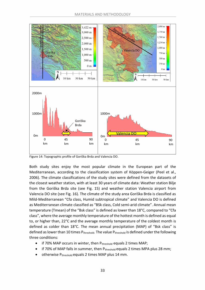
MATERIALS AND METHODOLOGY
33
Figure 14: Topographic profile of Goriška Brda and Valencia DO.
Both study sites enjoy the most popular climate in the European part of the
Mediterranean, according to the classification system of Köppen-Geiger (Peel et al.,
2006). The climate classifications of the study sites were defined from the datasets of
the closest weather station, with at least 30 years of climate data: Weather station Bilje
from the Goriška Brda site (see Fig. 15) and weather station Valencia airport from
Valencia DO site (see Fig. 16). The climate of the study area Goriška Brda is classified as
Mild-Mediterranean “Cfa class, Humid subtropical climate” and Valencia DO is defined
as Mediterranean climate classified as “BSk class, Cold semi-arid climate”. Annual mean
temperature (Tmean) of the “Bsk class” is defined as lower than 18°C, compared to “Cfa
class”, where the average monthly temperature of the hottest month is defined as equal
to, or higher than, 22°C and the average monthly temperature of the coldest month is
defined as colder than 18°C. The mean annual precipitation (MAP) of “Bsk class” is
defined as lower than 10 times Pthreshold. The value Pthreshold is defined under the following
three conditions:
• if 70% MAP occurs in winter, then Pthreshold equals 2 times MAP;
• if 70% of MAP falls in summer, then Pthreshold equals 2 times MPA plus 28 mm;
• otherwise Pthreshold equals 2 times MAP plus 14 mm.
1000mm
2000m
0m 0 km
45 km
90 km
Goriška Brda
0m
1000m
90 km
45 km
0 km
Valencia DO

MATERIALS AND METHODOLOGY
34
The values of MAP under “Bsk class” are lower, compared to “Cfa class”, which is defined
as a class without a dry summer nor a dry winter. A dry summer is defined under two
conditions: precipitation in the driest month is lower than 40 mm and where the
precipitation of the driest month is lower than a third of the precipitation in the wettest
month in winter. A dry winter is defined, when precipitation in the driest month in
winter is lower than one tenth of the precipitation in the wettest month in summer. The
months October, November, December, January, February and March define winter and
the other six months define summer. The “Cfa class” characterises areas with lower
temperatures and approximately three times higher annual precipitation, compared to
“Bsk class” (Peel et al., 2006).
2.3 Meteorological data
The meteorological data were retrieved from the weather stations located within the
borders of both study sites and in the surrounding areas. The parameters used were:
daily minimum temperature (Tmin), daily Tmax, daily Tmean, daily precipitation,
evapotranspiration and number of sun hours per day.
Meteorological datasets in Goriška Brda
For the spatial-temporal analysis in the Goriška Brda study site, eleven weather stations
were used. These were located inside the study site or in close proximity to it (see Fig.
15).
Figure 15: Study site Goriška Brda (area coloured in red) and location of available weather stations.

MATERIALS AND METHODOLOGY
35
There are nine weather stations within the borders of Slovenia and two in Italy: Lignano
and Fossalon. The stations were chosen according to their location and recorded data
history. The selected stations were chosen under the following three conditions:
1. Location of station should to be within the study area of Goriška Brda or no more
than 60 km from the weather station Vedrijan, located inside of the Goriška Brda
study site. The meteorological station Koper is the farthest station from Vedrijan
(approx. 54 km).
2. Station should record daily meteorological parameters.
3. Station should have been recording data for a minimum of 15 years.
The weather stations Lignano, Fossalon and Bilje were chosen due to their proximity to
the coast, to analyse the influence of the Mediterranean Sea on climate in the study site.
The weather station Vogel is the highest located station at 1922 m asl. It was chosen for
its proximity to the study site and the altitude temperature analysis. The remaining
stations were chosen due to their proximity to the study area and their long-year
historical dataset. The meteorological data from the stations located in Slovenia were
gathered from the Ministry of the environment and spatial planning of the Republic of
Slovenia (Arso, 2017). The data from the stations positioned in Italy were gathered from
the Regional Meteorological Observations of Italy (Meteo.fvg, 2019). A temporal
variability in the recorded period amongst the weather stations was noticed in the whole
study site (see Table 3).
Table 3: Data of used weather stations in the study site Goriška Brda.
Station
name
Available
daily data
Latitude
(°)
Longitude
(°)
Elevation
(m)
Approx. distance from
Mediterranean Sea (km)
Bilje 1962-2016 45.8867 13.6364 52 20
Vojsko 1961-2016 46.0206 13.9080 1083 36
Vogel 1982-2016 46.2592 13.8458 1922 75
Nova
Gorica
1970-2000 45.9512 13.6572
104 21
Godnje 1960-2016 45.7504 13.8502 304 10
Vedrijan 1960-1990 46.0120 13.5503 248 25
Nanos 1966-2001 45.8120 14.0169 904 22
Postojna 1961-2016 45.7618 14.1977 556 37
Koper 1950-1975 45.5287 13.7336 20 7
Lignano 1999-2016 45.7050 13.1469 15 5
Fossalon 1999-2016 45.7179 13.4587 12 4
From all weather stations in Goriška Brda study site the temperature parameters were
measured three times per day: at 7:00, 14:00 and 21:00 hrs. Daily Tmean was calculated
according to the three measurements during each day (Arso, 2017).

MATERIALS AND METHODOLOGY
36
Meteorological datasets in Valencia DO
In the Valencia DO study site were used eight meteorological stations located within the
Valencia DO study site and the surrounding area (Fig. 19).
Figure 16: Location of weather stations in and around the study site Valencia DO.
The selected stations were chosen under following three conditions:
1. Location of station should be within the study area Valencia DO or no further
than 120km from the weather station Cheste, located within the study site. With
a distance of 116km, Abacete weather station is the furthest away from Cheste.
2. Station should record daily meteorological parameters stated below.
3. Station should have been recording for a minimum period of 15 years.
Applying the stated conditions, the stations Llíria and Cheste were chosen due to their
central location in the viticultural area of Valencia DO (Table 4). To improve the spatial-
climate analysis of the study site, and the impact of the Mediterranean Sea, were chosen
the stations, which are located between the coastline and Valencia DO: Valencia airport,
Castellón and Benifaió. The locations of the weather stations Albacete, Cerrito Requena

MATERIALS AND METHODOLOGY
37
and Teruel are located in inland not far from the study site. They were also chosen to
enhance the spatial-climate analysis of the Valencia DO site. The parameters used from
the weather stations were the same as the ones used from the study site Goriška Brda.
Table 4: Data of used weather stations at the study site Valencia DO.
Station
name
Available
daily data
Latitude
(°)
Longitude
(°)
Elevation
(m)
Approx. distance from
Mediterranean Sea
(km)
Valencia
airport
1965-
2016 39.4867 -0.4735 69 14
Albacete 1914-
2016 38.9502 -1.8500 686 140
Castellón 1937-
2016 39.9892 -0.0406 30 9
Benifaió 1999-
2016 39.2806 -0.4619 35 12
Teruel 1986-
2016 40.3497 -1.1169 915 104
Requena Cerrito
2000-
2016 39.5047 -1.2324 810 57
Lliria 2000-
2016 39.6910 -0.6270 250 28
Moncada 2000-
2016 39.5877 -0.3990 35 8
Cheste 1999-
2014 39.5189 -0.7445 110 31
The weather stations in Valencia DO site measured the temperature twice daily: at 6:00
and 18:00 hrs. Daily Tmean was calculated as an average of the daily maximum and
minimum temperature (Ecad, 2016). Datasets from defined meteorological stations
were used for calculations of bioclimatic indices, Tmin frequency, delineation and WR
analysis. The usage of each dataset from each weather station in this thesis is described
in Table 5.

MATERIALS AND METHODOLOGY
38
Table 5: Used datasets from weather stations used in this thesis presented for each type of analysis and in which of the six analyses they were used. Grey cells represent the involvement of the weather station’s datasets.
Stu
dy
site
Station name
Bioclimatic indices
Other analysis Analysis number
Hu
glin
ind
ex
Win
kle
r in
dex
Dry
nes
s in
dex
Tem
per
atu
re
Pre
cip
itat
ion
Tmin
fre
qu
ency
De
linea
tio
n
Wat
er
req
uir
eme
nt
An
alys
is 1
An
alys
is 2
An
alys
is 3
An
alys
is 4
An
alys
is 5
An
alys
is 6
Go
rišk
a B
rda
Bilje
Vojsko
Vogel
Nova Gorica
Godnje
Vedrijan
Nanos
Postojna
Lignano
Fossalon
Val
en
cia
DO
Valencia airport
Albacete
Castellón
Benifaió
Teruel
Requena Cerrito
Lliria
Cheste
Moncada
Campo Arcis
The daily precipitation data were retrieved from one meteorological station from each
study site: Bilje in the Goriška Brda (see Fig. 15) site and Valencia airport in the Valencia
DO (see Fig. 16). Both weather stations were chosen due to their long historical dataset
and closeness to the study sites.
Missing data
In some cases, weather stations failed to record daily meteorological parameters,
usually due to technical problems. Some of the used weather stations experienced
technical disturbances for one day or more. In these cases, the methodology of linear

MATERIALS AND METHODOLOGY
39
regression was used to calculate the missing data, using the datasets of the closest
weather station, which possessed the data from the missing time range (Ferreri & Ozaki,
2014). The methodology of reconstructing the missing data in daily datasets was used
to evaluate the most probable values and so there is a measure of uncertainty.
For the linear regression analysis, the temperature datasets of two weather stations
were used. The first temperature dataset was derived from the weather station with
missing data. The second temperature dataset was derived from the topographically
closest weather station, which contained the temperature data for the missing dates.
The longest data period was chosen, where there was no missing data provided by both
stations. From the chosen temperature dataset, was calculated the coefficient of
determination (Cornell & Berger, 1987), also called the multiple correlation coefficient
R2, using the Eq. (1). The value of the coefficient of determination is a measure of the
strength of the correlation between various datasets. In this thesis were compared two
datasets from two weather stations. The value R2 was between 0 and 1. Values of R2
closer to 1 mean a stronger correlation and vice versa. R2 stands for coefficient of
determination, n stands for the number of days included in the statistical analysis which
calculates the R2, yi stands for the daily temperature variable of the station with the
missing dataset, yi stands for the daily temperature variable of the station without
missing data and y stands for the Tmean of the station with the missing data.
𝑅2 =
∑ (��𝑖 − ��)2𝑛𝑖=1
∑ (𝑦𝑖 − ��)2𝑛𝑖=1
(1)
If R2, revealed a value lower than 0.8, the second closest weather station was found,
until the condition (R2>0.8) is fulfilled. This case did not occur in this thesis. The
substitution of the missing data was done with a linear adjustment, using the linear
equation of the trendline (Tardivo & Berti, 2012). This procedure was used for Tmin,
Tmax and Tmean datasets. The missing precipitation data were filled with the data from
the closest station containing the missing data. The calculations of bio-climatic indices
HI and WI (Huglin, 1978; Anderson et al., 2012) were conducted with the temperature
datasets, which did not include more than seven consecutive days with no daily
temperature data during the analysis period of each bioclimatic index. Each bioclimatic
index uses its own analysis period, which generally corresponds to the growing season
of grapevine in the Northern Hemisphere. In the event of missing data longer than seven
consecutive days, the bioclimatic index of that particular year was not included in the
further analysis. Among eleven weather stations were used in the Goriška Brda site,
there were encountered five weather stations with more than eight consecutive days
with missing temperature data during growing season (see Table 6).
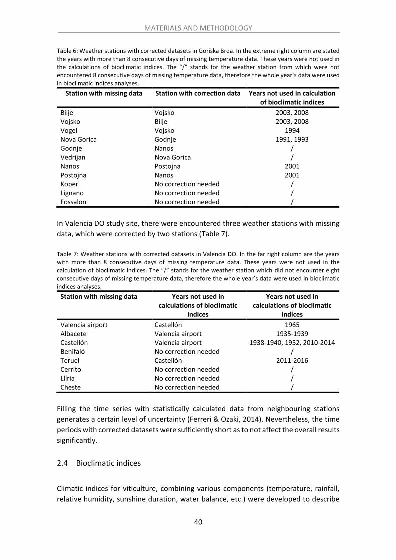
MATERIALS AND METHODOLOGY
40
Table 6: Weather stations with corrected datasets in Goriška Brda. In the extreme right column are stated the years with more than 8 consecutive days of missing temperature data. These years were not used in the calculations of bioclimatic indices. The “/” stands for the weather station from which were not encountered 8 consecutive days of missing temperature data, therefore the whole year’s data were used in bioclimatic indices analyses.
Station with missing data Station with correction data Years not used in calculation of bioclimatic indices
Bilje Vojsko 2003, 2008 Vojsko Bilje 2003, 2008 Vogel Vojsko 1994 Nova Gorica Godnje 1991, 1993 Godnje Nanos / Vedrijan Nova Gorica / Nanos Postojna 2001 Postojna Nanos 2001 Koper No correction needed / Lignano No correction needed / Fossalon No correction needed /
In Valencia DO study site, there were encountered three weather stations with missing
data, which were corrected by two stations (Table 7).
Table 7: Weather stations with corrected datasets in Valencia DO. In the far right column are the years with more than 8 consecutive days of missing temperature data. These years were not used in the calculation of bioclimatic indices. The “/” stands for the weather station which did not encounter eight consecutive days of missing temperature data, therefore the whole year’s data were used in bioclimatic indices analyses.
Station with missing data Years not used in calculations of bioclimatic
indices
Years not used in calculations of bioclimatic
indices
Valencia airport Castellón 1965 Albacete Valencia airport 1935-1939 Castellón Valencia airport 1938-1940, 1952, 2010-2014 Benifaió No correction needed / Teruel Castellón 2011-2016 Cerrito No correction needed / Llíria No correction needed / Cheste No correction needed /
Filling the time series with statistically calculated data from neighbouring stations
generates a certain level of uncertainty (Ferreri & Ozaki, 2014). Nevertheless, the time
periods with corrected datasets were sufficiently short as to not affect the overall results
significantly.
2.4 Bioclimatic indices
Climatic indices for viticulture, combining various components (temperature, rainfall,
relative humidity, sunshine duration, water balance, etc.) were developed to describe

MATERIALS AND METHODOLOGY
41
each region’s viticultural potential. The bioclimatic indices HI and WI were calculated,
with the purpose of defining general guidelines for the potential quality and style of
wine (Winkler et al., 1974; Briche et al., 2014) and the DI to assess the water availability
in the soil (Riou et al., 1994; Tonietto & Carbonneau, 2004). HI is derived from the
observed or simulated daily temperature in a certain period and is correlated with wine
growth and sugar concentration in berries. It is classified into six HI classes, where each
class suggests a grape variety according to the number of points in a class (see Table 8).
Table 8: HI classes with corresponding suggested grape varieties (Tonietto and Carbonneau 2004).
Huglin class
Class points Suggested grape varieties
Very cold ≤ 1500
Only the early cultivars that can reach maturity, especially the white varieties (i.e. Muller-Thurgau, Pinot blanc, Gamay and Gewurztraminer)
Cold 1500-1800 Riesling, Pinot noir, Chardonnay, Merlot and Cabernet franc Cool 1800-2100 Cabernet-Sauvignon, Ugni Blanc and Syrah Warm 2100-2400 Grenache, Mourvèdre and Carignan Hot 2400-3000
Potential which exceeds the heliothermal needs to ripen the varieties, even the late ones (with some associated risks of stress).
Very hot >3000 There is no heliothermal constraint for the grapes to ripen.
It is calculated according to Eq. (2) for each year from April to September in the Northern
Hemisphere. The sum of the daily Tmean and daily Tmin is more than 10°C (Huglin,
1978). If the sum was less than 10°C, zero HI points were designated for that particular
day. The day length coefficient k, which is defined according to the latitude, was defined
as 1.02 for Valencia DO and 1.04 for the Goriška Brda study site. Coefficient k is defined
by geographical latitude (Tonietto and Carbonneau, 2004).
𝐻𝐼 = ∑(Tmean − 10) + (Tmax − 10)
2
30 sep
1 apr
∙ k
(2)
The WI estimates the characteristics of geographical zones and the local adaptation of grape varieties (Winkler et al., 1974). It is classified into five different regions with designated suggested grape varieties (Table 9). Table 9: WI regions with recommended grape varieties (Tonietto & Carbonneau 2004).
Winkler regions Class points Suggested grape varieties
Region 1 850-1389 Pinot noir, Riesling, Chardonnay, Gewurztraminer, Pinot grigio and Sauvignon blanc
Region 2 1389-1667 Cabernet sauvignon, Chardonnay, Merlot, Semillon, Syrah
Region 3 1671-1950 Grenache, Barbera, Tempranillo and Syrah Region 4 1951-2220 Carignan, Cinsault, Mourvedre and Tempranillo Region 5 >2221 Primitivo, Nero d’avola, Palomino and Fiano

MATERIALS AND METHODOLOGY
42
It is calculated according to Eq. (3) for each year from April to October. The days with a Tmean of less than 10°C were given zero WI points. The threshold of 10°C was adopted, due to phonologically activity, which begins when daily Tmean exceeds 10°C (Huglin & Schneider, 1998). Tmean stands for daily Tmean and Tmin stands for daily Tmin (Tonietto & Carbonneau, 2004).
𝑊𝐼 = ∑ (𝑇𝑚𝑒𝑎𝑛 − 10°𝐶)
31 𝑜𝑐𝑡
1 𝑎𝑝𝑟
(3)
The DI is defined according to the adaptation of the potential water balance of the soil index of Riou (Riou et al., 1994). It was developed to assess potential water availability in soil, for viticulture purposes (Fraga, 2014). It is calculated by using the initial useful water reserve accessible by the roots, the amount of precipitation, the potential plant transpiration and the direct soil evaporation (Tonietto & Carbonneau, 2004), as defined in Eq. (4). Daily data for evapotranspiration and daily precipitation for the Goriška Brda study site were retrieved from the Ministry of the environment and spatial planning of the Republic of Slovenia (Arso, 2017). The same climatic parameters were retrieved from the Valencia DO study site from the Instituto Valenciano de Investigaciones Agragarias (IVIA, 2017).
𝑊 = 𝑊0 + 𝑃 − 𝑇𝑣 − 𝐸𝑆
(4)
𝑊 stands for estimation of soil water reserve defined for the six month period. 𝑊0
stands for initial useful soil water reserve which is accessible by the roots. According to
the definition of the DI, the 𝑊0 should not exceed 200 mm. 𝑃 stands for amount of
precipitation per month in mm, 𝑇𝑣 stands for potential transpiration and 𝐸𝑆 in Eq. (5),
stands for direct evaporation from the soil. 𝐸𝑇𝑃 stands for monthly total of potential
evapotranspiration using the Penman method (Penman, 1948) and 𝑘 stands for
coefficient of radiation absorption by vine plant. For the Northern Hemisphere, where
both study sites are located, the value 𝑘 was adopted as value 0.1 for April, 0.3 for May
and 0.5 for June, July, August and September.
𝑇𝑣 = 𝐸𝑇𝑃𝑘
(5)
In Eq. (6) is given the definition of 𝐸𝑆, where 𝐸𝑇𝑃 stands for monthly total of potential
evapotranspiration, 𝑁 stands for number of days in the month and 𝐽𝑃𝑚 stands for the
number of days of effective evaporation from the soil per month. Value of 𝐽𝑃𝑚 is
defined equal or lower of the number of days per month.
𝐸𝑆 =
𝐸𝑇𝑃
𝑁 (1 − 𝑘)𝐽𝑃𝑚
(6)

MATERIALS AND METHODOLOGY
43
According to the definition of the DI (Tonietto & Carbonneau, 2004), the 𝑊0 should not
exceed the value of 200 mm and 𝑊 should not be more than 𝑊0. The DI is divided into
four specific classes, according to the value of the index (see Table 10).
Table 10: Definition of DI classes.
DI class Class interval Acronym
Very dry ≤ – 100 DI + 2 Moderately dry ≤ 50 and >- 100 DI + 1 Sub-humid ≤ 150 and > 50 DI – 1 Humid > 150 DI – 2
Descriptions of each DI class adopted by Tonietto and Carbonneau (2004):
• Very dry areas experience an extensive lack of water resources, which leads to
frequent hydric stress. Grapevine needs irrigation to grow. Areas with lower than
-100 mm of DI are characterised as having a high water deficit. The regions
characterized with -200 mm are defined as having a high deficit of available
water. Plant can suffer severe stress, if not sufficiently irrigated. Examples of
these wine areas are: Jerez de la Frontera (Spain), Ica (Peru) and Nuriootpa
(Australia).
• In Moderately dry areas, a plant can potentially suffer frequent dryness.
Irrigation is applied in most cases. Plants experience significant stomatal
regulation, which is beneficial for maturation process. Irrigation is used in some
cases. The regions defined with a DI less than 50 mm, are classified as
Mediterranean type climate, exposed to water deficit. Examples of these areas
are Montpellier (France) and Madeira (Portugal).
• Sub-humid areas experience absence of dryness. The minimum threshold of 50
mm is a critical value in defining the minimum water balance for the vine plant
during periods of frequent summer dryness. Consequently, it is a good indicator
to characterize areas with absence or presence of frequent dryness. Examples of
these wine regions are Bordeaux, Napier (New Zealand), Reims (France) and
Champagne (France).
• The Humid class areas experience high absence of dryness, with high availability
of water resources. The excess of water balance can affect the quality of the
yield. Best grape quality is achieved in less humid years. Examples of these wine
areas are: Bento Gonçalves (Brazil), Serra Gaúcha (Brazil), Freiburg (Germany),
Macon (France) and Bourgogne (France).
2.5 Minimum temperature frequency
Cool and extreme hot temperatures influence the initiation of biological processes of
the vine (Creasy & Creasy, 2009). Furthermore, the viticultural potential is defined by

MATERIALS AND METHODOLOGY
44
various components, especially by Tmean, Tmax and Tmin (Deloire et al., 2005), which
is particularly important in the ripening season of vine. The minimum frequency
temperature was calculated for two periods: in the year 2000 and in the year 2016. The
time periods were chosen due to the availability of meteorological data at the maximum
number of weather stations in Goriška Brda and Valencia DO viticulture sites. The margin
of 2°C was chosen for calculations to better understand the temperature frequency, the
same as in the study of Bonnardot (2012).
2.6 Datasets of future climate scenarios
The aim of this thesis is to conduct research under two scenarios, creating margins
between the most “optimistic” and the most “pessimistic” scenarios. The scenario
RCP2.6 is defined as too “optimistic” for the type of future analysis conducted in this
thesis, therefore, scenario RCP4.5 was chosen as the optimistic scenario. It is known by
its low-emission nature and it should stabilize the concentration of radiative forcing at
approx. 4.5 W/m2 by the year 2150 (Van Vuuren et al., 2011). The RCP8.5 scenario was
chosen due to its nature of modelling the future in the upper margin and is the
pessimistic future scenario. It represents a ‘do nothing against the climate change’
scenario. It is also called “the worst case scenario” (Wayne, 2013). Stabilizing
concentration of radiative forcing should be achieved at approx. 12 W/m2. The RCP6 was
not considered in this study due to its ‘middle of the road’ nature, being between RCP4.5
and RCP8.5 scenario. By using scenarios RCP4.5 and RCP8.5, it was possible to analyse
two alternative futures and create the most likely future between the chosen margins.
Regional Climate Models (RCM) were chosen due to their higher spatial resolution,
compared to the General circulation models. Datasets of future climate scenarios used
in thesis, were retrieved from two sources, due to their different spatial resolution and
different reference and future projection periods: Worldclim (Hijmans et al., 2005) and
Euro-Cordex (Jacob et al., 2014; Euro-Cordex, 2017).
Worldclim data were used in temperature analysis in the Goriška Brda site (see 2.8.1).
The dataset was retrieved within the framework of the CMIP5 dataset, for two periods:
reference period 1950-2000 and future period 2041-2060. The future dataset of average
monthly Tmin and Tmax was used under RCP4.5 and RCP8.5 scenarios. The data were
downloaded from tile 16 with a 30 arc-second resolution grid. With the GIS tool were
obtained the temperature dataset for each location of the three weather stations
included in this analysis. The dataset Worldclim was chosen due to its high resolution
(30 arc-second grid, approx. 1 km x 1 km) (see Table 11).

MATERIALS AND METHODOLOGY
45
Table 11: Descriptions of climate model datasets used in this thesis. Analysis number refers to an analysis number specific to this thesis.
Model datasets
Spatial resolution
Analysis period
Purpose Analysis number
Study site
Worldclim 1 km x 1 km
1950-2060
• Elaboration of the future temperature model
2 Goriška Brda
Euro-Cordex
12.5 km x 12.5 km
1985-2100
• Elaboration of the future temperature model
• Bioclimatic indices analysis
• WR analysis
3,4 and 6
Goriška Brda and Valencia DO
The CORDEX datasets were used from the RCM simulations used in Europe, called Euro-
Cordex (Vautard et al., 2013). It offers two spatial resolutions: 0.44 degree (approx.
50km x 50km) and 0.11 degree (approx. 12.5km x 12.5km). Using the Euro-Cordex (Euro-
Cordex, 2017) internet site, the datasets for the RCP4.5 and RCP8.5 scenarios were
downloaded. The datasets for scenarios RCP4.5 and RCP8.5 were retrieved for the
location of each station by using the statistical software tool R (Robitzsch et al., 2019).
The dataset contained the following climate parameters and time periods: daily Tmin
(1985-2100), daily Tmax (1985-2100) and daily precipitation (1985-2100). In the
reference period 1985-2005, the dataset included one scenario. In the period 2005-2100
were retrieved the RCP4.5 and RCP8.5 scenarios. In each analysis a particular
methodology was used applying different input datasets, study periods, climate models
and calculated parameters (see Table 12).

MATERIALS AND METHODOLOGY
46
Table 12: Overview of input data and outcomes for each analysis in this thesis. The weather stations used in each analysis are described in Table 5.
Analysis name Study site
Period Model datasets Calculated parameters
A1: Historical spatial-temporal analysis of temperature and Dryness index (1965-2013)
Goriška Brda and Valencia DO
1965-2013
/ Temperature, HI, WI, DI and Tmin frequency.
A2: Future temperature modelling in Goriška Brda study site (2041-2060)
Goriška Brda
1950-2060
Worldclim Temperature.
A3: Spatial-temporal analysis of temperature and bioclimatic indices (1965-2100)
Goriška Brda and Valencia DO
1965-2100
Euro-Cordex Temperature, HI and WI.
A4: Spatial-temporal analysis of temperature and precipitation (1985-2100)
Goriška Brda and Valencia DO
1985-2100
Euro-Cordex Temperature and precipitation.
A5: Assessment of viticultural potential and delineation in Goriška Brda
Goriška Brda
/ / Map of homogeneous viticultural zones with their viticultural potential.
A6: Assessment of WR in Valencia DO (1985-2100)
Valencia DO
1985-2100
Euro-Cordex WR for Tempranillo, Bobal and Moscatel.
2.7 Analysis 1: Historical spatial-temporal analysis of temperature and
bioclimatic indices (1965-2013)
The purpose of this part of this analysis is to provide an analysis of temperature, and
influence of the sea on Goriška Brda and Valencia DO for the period 1965-2013. Both
viticulture sites share similar topographical conditions (see Fig. 14) and benefit from,
and are influenced by the Mediterranean Sea’s climate as they are approx. 80km from
the Mediterranean coastline. According to their length of historical data and proximity
to the study sites, four weather stations were chosen. In each site, it was chosen one
weather station between the study site and the Mediterranean coastline and the second
one further away from the study area, more inland. In Goriška Brda were used two
additional meteorological stations. Station Bilje lies approx. 14km from the coastline of
the Mediterranean Sea and Vojsko approx. 35km from the Mediterranean coastline (see
Fig. 15). In the Valencia DO study site were chosen two meteorological stations. Station
Valencia airport is located approx. 13 km and Albacete approx. 140 km from the
Mediterranean coastline (see Fig. 16). From each meteorological station, was retrieved
the temperature dataset for the historical period 1965-2013. Furthermore, the spatial

MATERIALS AND METHODOLOGY
47
analysis of bioclimatic index DI and minimum temperature were conducted in both
study site for the period 2000-2016.
Temperature statistical analysis
The historical temperature model was elaborated, using the historical temperature data
from both study sites. It represents the temperature progress from four weather
stations during the last five decades in both study sites. From each meteorological
station were retrieved daily Tmin, Tmax and Tmean. At all four weather stations, daily
Tmean was calculated according to several daily measurements. In Slovenia’s site, each
day three measurements were performed: at 7:00, 14:00 and 21:00 hrs. The data were
retrieved from the Slovenian Environment Agency (Arso, 2017). From the three daily
measurements, the minimum and the Tmax were selected. Daily Tmean was calculated
from the daily three measurements. At the site in Spain, there two daily measurements
were performed: at 6:00 and 18:00 hrs. Data were retrieved from the European Climate
Assessment and Dataset (Ecad, 2016). From the two daily measurements, the minimum
and the Tmax were selected. Daily Tmean was calculated from daily measurements. For
defining tendency of annual temperatures during the analysis period, was used linear
regression. The temperature fluctuation at all four weather stations was compared to
define the spatial temperature variability and possible impact of water masses like the
Mediterranean Sea.
Bioclimatic indices statistical analysis
The HI and WI bioclimatic indices (Tonietto & Carbonneau, 2004) (see 2.4) were
calculated, using the daily temperature data for the period 1965-2013. The tendency of
both bioclimatic indices was defined with linear regression. Using bioclimatic indices,
the temporal and spatial variety of suggested grape varieties were defined in both study
sites. The comparison analysis was performed, to define differences between the two
viticultural areas.
Spatial-temporal analysis of minimum temperature frequency analysis
Spatial analysis of daily Tmin ranges was conducted in both viticultural sites, to analyse
the optimum night temperature requirements for colour and flavour development of
berries (Bonnardot et al., 2012). The analysis was conducted in both study sites using
datasets from seven weather stations from each site (see Table 5). In the study site
Goriška Brda, were used the following weather stations: Vogel, Vojsko, Postojna,
Godnje, Bilje, Fossalon and Lignano (see Fig. 15). In the study site Valencia DO, were
used the following weather stations: Valencia_airport, Albacete, Llíria, Castellon,
Benifaió, Cheste and Teruel (see Fig. 16). Input data in this analysis were daily Tmin. For
spatial-temporal analysis of Tmin frequency, years 2000 and 2016 were selected.

MATERIALS AND METHODOLOGY
48
Spatial-temporal analysis of Dryness Index
The potential water balance of the soil was analysed in both viticultural sites for the
period 2000-2016, using the bioclimatic index DI (see 2.4). Three weather stations were
chosen from each study site (see Table 5) due to their available datasets and closeness
to the study areas: Postojna, Bilje and Godnje in Goriška Brda (see Fig. 15) and Llíria,
Cheste and Benifaió in Valencia DO site (see Fig. 16). Similar DI analysis was conducted
on other viticultural areas in Europe and Africa for the periods 1980-2009 and 1950-
1979 (Santos et al., 2013), however in this thesis, the analysis was conducted on a local
scale.
2.8 Analysis 2: Future temperature modelling in Goriška Brda study site (2041-
2060)
Objective of this research is to conduct temperature analysis of temperature model and
observed temperature during the last five decades in the Goriška Brda viticultural site
by using the Worldclim datasets, which was also used in the same study site in Analysis
5 (see 2.11). Therefore, this analysis was conducted only in Goriška Brda due to the
comparison analysis between the lower (Euro-Cordex) and higher (Worldclim) spatial
resolution and to define the correlation between them. Observation data were retrieved
from three weather stations in the Goriška Brda site: Vedrijan, Bilje and Vojsko (see
Table 5 and Fig. 15). From the meteorological stations were retrieved observed daily
minimum and Tmax for specific periods. Each weather station recorded air temperature
daily at 7.00, 14:00 and 21:00 hrs. From the three-daily data, minimum and Tmax were
selected. Depending on the available daily temperature datasets from each station, the
periods of observation datasets were chosen differently. From Vojsko station were
retrieved data for the period 1961-2000, Bilje for the period 1962-2000 and Vedrijan for
the period 1960-1990. Data from the weather stations were retrieved from the Ministry
of Environment and spatial planning of Republic of Slovenia (Arso, 2017). There were no
available meteorological data before the year 1961 in the above mentioned weather
stations. The temperature analysis was conducted using the observed temperature data
from the three meteorological stations and the Worldclim dataset for the period 1950-
2000. For the comparison between observed and Worldclim data, the average monthly
temperature was calculated, using the mathematical average of daily measurements.
With the gathered temperature data for the time period 1950-2000, the observed
weather station data was compared with modelized data from the Worldclim dataset.
The future temperature simulation was calculated from the observation data on each
weather station. From the comparison analysis of modelized and observation data for
the period 1950-2000, it was calculated the function to calculate the future scenario for
the time period 2041-2060. Afterwards, the comparative analysis between observed
(1950-2000) and future modelized (2041-2060) temperatures was conducted at each
weather station. The averages of monthly temperatures in all three weather stations
were calculated and compared between future simulated and observation data.

MATERIALS AND METHODOLOGY
49
Future modelling calculations
Input data used in this analysis were from two sources. Observed monthly temperature
datasets of maximum and minimum average monthly temperature were retrieved from
all three meteorological stations for the defined time periods. Modelized data were
retrieved from the Worldclim dataset. For each station were retrieved modelized
datasets under RCP4.5 and RCP8.5 scenarios for the period 2041-2060. The average
maximum monthly temperature was calculated at each meteorological station, using
available observation data in the period 1962-2000. The monthly average Tmax was
calculated from all three stations. From the modelized Worldclim dataset, it was
calculated the average monthly Tmax for two periods: 1950-2000 and 2041-2060 in each
weather station. Afterwards, the monthly average Tmax was calculated from all three
stations for the periods 1950-2000 and 2041-2060. For calculation of future monthly
Tmax in Eq. (7), it was used the correction value 𝑘, which defines the correction factor
between observed and modelized average monthly Tmax. Tmax_m_b stands for
modelized average monthly temperature for the period 2041-2060, Tmax_m_a stands for
modelized average monthly temperature for the period 1950-2000 and k stands for
correction factor.
𝑘 =𝑇𝑚𝑎𝑥_𝑚_𝑎
𝑇𝑚𝑎𝑥_𝑚_𝑏
(7)
The corrected average monthly Tmax was calculated by using the correction factor 𝑘 in
Eq. (8). Tmax _c_b stands for average monthly Tmax for the period 2041-2060, k stands
for correlation factor defined in (7) and Tmax _o_a stands for average observed monthly
Tmax for the period 1950-2000.
𝑇max _𝑐_𝑏 = 𝑘𝑇max _𝑜_𝑎
(8)
The same calculations were used to calculate the corrected average monthly Tmin. The average was calculated using the mathematical average of Tmin and Tmax. It was conducted spatial-temporal analysis using temperature observations and calculated temperature model.
2.9 Analysis 3: Spatial-temporal analysis of temperature and bioclimatic indices
(1965-2100)
Objective of this research is to conduct a critical analysis of the last five decades of
temperature data in both study sites, by using daily temperature data from the three
weather stations. The second objective was to elaborate the future climate model under
RCP4.5 and RCP8.5 scenarios, until the year 2100 on a local scale. The third objective
was to elaborate on two future models to determine grape varieties suitable to grow
during the period 1985-2100. One of the future models was defined by bioclimatic
indices HI and the second one with WI. The choice of weather stations was made
according to the longest available historical datasets of temperature and the location

MATERIALS AND METHODOLOGY
50
rule: at least one station had to be located close to the seacoast and another in the
countryside. In Goriška Brda site were selected three (Vojsko, Godnje and Bilje) and in
Valencia DO one weather station (Valencia airport) (see Table 5, Fig. 15 and Fig. 16), with
daily temperature datasets from 1965 onwards. In the further analysis, the Tmean
values were used from the three weather stations. From the retrieved daily data, daily
maximum and minimum temperatures were defined. Daily Tmean was calculated from
the three measurements each day. Modelized data were retrieved from the Euro-
Cordex data base (Euro-Cordex, 2017). The Dataset contained the daily Tmin and Tmax
for the reference period 1985-2005 and future RCP4.5 and RCP8.5 scenarios for 2005-
2100 (IPCC, 2014). Average daily temperature value was calculated by using the
mathematical mean from daily maximum and minimum temperatures.
The calculations for bioclimatic indices HI and WI are explained in section 2.4 and 2.5. In
addition to absolute temperature analysis, temperature anomaly was used to determine
the temperature progress during the analysis period. Temperature anomalies are most
used in future sceneries (Hidore et al., 2010). In Eq. (9), ∆𝑇 stands for temperature
anomaly, 𝑇𝑖 stands for measured temperature and Tmean stands for average
temperature of the reference value (IPCC, 2007).
∆𝑇 = 𝑇𝑖 − 𝑇𝑚𝑒𝑎𝑛
(9)
The reference value is defined as a 30 year long period, which defines the climate
(Arguez & Vose, 2011). The reference period defined in this analysis, was from 1965 to
1993.
2.10 Analysis 4: Spatial-temporal analysis of temperature and precipitation
(1967-2100)
The objective of this research is to provide a critical and comparative analysis of
temperature during the observation period (1985-2016), and to elaborate on future
scenarios RCP4.5 and RCP8.5 for both study sites. In order to conduct the spatial-
temporal analysis, fifteen weather stations were determined. Seven from the study site
Valencia DO (Albacete, Requena, Cheste, Llíria, Valencia airport, Teruel and Castellón)
and eight from the Goriška Brda site (Lignano, Vedrijan, Bilje, Nova Gorica, Godnje,
Vogel, Vojsko and Nanos) (see Table 5, Fig. 15 and Fig. 16). The input datasets observed
in this analysis were daily Tmin and Tmax from each weather station for the period 1985-
2016 and modelized daily Tmin and Tmax for each weather station. Modelized data were
retrieved from the Euro-Cordex dataset (Euro-Cordex, 2017). It contained daily Tmin and
Tmax for the reference period 1985-2005 and future RCP4.5 and RCP8.5 scenarios for
2005-2100. Tmean values were calculated using the mathematical mean from the Tmin
and Tmax values. The analysis was conducted in two stages. For the spatial-temporal
analysis of each study site, the observation datasets daily Tmin, Tmax and Tmean were
retrieved from every participating weather station and utilised in this analysis for the
period 1985-2016. Using the modelized daily Tmin, Tmax and Tmean data, the spatial-
temporal analysis was conducted in both study areas for the period 1985-2100.

MATERIALS AND METHODOLOGY
51
The comparison analysis between both study sites is presented in the second part. The
daily mean values of daily Tmin, Tmax and Tmean for observed and modelized datasets
were calculated using datasets from the weather station Bilje in the Goriška Brda study
site. The same methodology was used in the Valencia DO study area, using the Valencia
airport weather station. In the analysis period 1985-2016, there were two types of
dataset: observed and modelized. In order to compare both datasets, the correlation
analysis between the two data types was conducted, to define the strength of
correlation. From both data types, the annual average absolute temperature difference
was calculated by Eq. (10). Absolute temperature difference was calculated for annual
Tmin, Tmax and Tmean. Tobs stands for annual average observed temperature, Tmod
stands for annual average modelized temperature.
𝑇𝑑𝑖𝑓𝑓𝑒𝑟𝑒𝑛𝑐𝑒 = |𝑇𝑜𝑏𝑠 − 𝑇𝑚𝑜𝑑|
(10)
To define the strength of correlation, the mathematical average of the 30 year period
(1985-2014) was used. Statistical and comparison analysis were conducted of both study
sites, using the observed and modelized mean annual temperature data for each study
site (minimum, maximum and average). The precipitation analysis was conducted for
the period 1967-2100 on two weather stations: Valencia airport (Valencia DO) and Bilje
(Goriška Brda) (see Fig. 15 and Fig. 16). Observation dataset for precipitation was
available from 1967-2016 and modelized dataset from 1985-2100.
2.11 Analysis 5: Assessment of viticultural potential and delineation in Goriška
Brda
The analysis of viticultural potential and suitability classification in this research is based
on fourteen environmental factors, which represent relief, climate and soil of the
viticultural area. They are: average annual temperature (AAT), average temperature of
the warmest month July (TWM), global radiation (GR), actual sunshine duration (ASD),
precipitation during the 6 months growing season (PP), sum of effective temperatures
(SET), length of the growing season (LGS), actual heliothermal index (IHa), oenoclimate
aptitude index (IAOe), clay content (Cly), humus content (Hum), soil skeleton/gravel
content (Gra), slope (S) and aspect (A). The growing season was defined as from the 1st
of April to the 30th of September (Huglin & Schneider 1998). These environmental
factors largely determine the viticultural potential and its spatial distribution in wine
regions located in temperate zones. The spatial dataset for the 14 environmental
parameters used in this study, was downloaded from the Ministry of the environment
and spatial planning of Slovenia (Surveying and Mapping Authority of the Republic of
Slovenia, 2019) and from the weather station Bilje in cooperation with the Slovenian
Environment Agency (Arso, 2017). The station Bilje was selected due to its available
historical climatic dataset and its proximity to the study site (see Fig. 17).

MATERIALS AND METHODOLOGY
52
Figure 17. Location of study site Brda, weather station Bilje and points where soil analysis was conducted. Gr. Ravne stands for Grgarske Ravne.
For spatial analysis, the classification of suitability ranking points of environmental
factors were adopted from the methodology by Irimia et al. (2014). The bioclimatic
viticultural index (Constantinescu, 1967) was excluded in the spatial analysis, because
previous results (González-Hidalgo et al., 2002; Irimia et al., 2014) showed that it was
not relevant in the assessment of viticultural potential of areas characterized by ‘Cfa’
climate (Peel et al., 2006). For each environmental factor was determined the suitability
class, ranked according to the production of different types of wine. The environmental
parameters were classified into four suitability classes: from the fourth class, not
suitable for viticulture, up to the first class, suitable for quality red wine production. The
precise representation of values of environmental factors and bioclimatic indices were
achieved by their annual averages (see Table 13).

MATERIALS AND METHODOLOGY
53
Table 13: Environmental parameters with defined suitability classes. Definitions and calculations of each
environmental parameter are given below.
Environmental categories
Environ-mental
parame-ters
Suitability classes†
IV III II I
Restrictive for
grapevine
White table wines, spar-
kling wines and wines for distillates
Quality white wines
Quality red wines
Climatic factors and bioclimatic indices
AAT (°C) <8.5 8.5-9.3 9.4-10.0 10.1-11.2 TWM (°C) <18.0 18.1-19.0 19.8-21.0 21.1-22.0 GR (kcal/cm2)
<80 80-83.9 84.0-86.9 87.0-92
ASD (hours) <80 80-83.9 84.0-86.9 87.0-92 PP (mm) 0 >390 <250 251-390 SET 1045-1675 <1045 1045-1200 1201-
1400 LGS (days) 160-210 <160 160-175 176-190 IHa 1.36-2.66 <1.36 1.36-1.70 1.71-2.20 IAOe 3793-4600 <3793 3793-4300 4301-
4600
Pedological factors
Cly (%) 6-40 >40 <15 25-40 Hum (%) 1.5-4.0 0 3.1-4.0 2.1-3.0 Gra (%) 0-40 >40 <10 30-40
Topographical factors
S (%) 0-28 0 <8 >15 A 0 0 NW, N, NE E, W
AAT, average annual temperature; TWM, average temperature of the warmest month; GR, global radiation; ASD, actual sunshine duration; PP, precipitation in the growing season; SET, sum of effective temperatures; LGS, length of the growing season; IHa, actual heliothermal index; IAOe, oenoclimatic aptitude index; Cly, clay content; Hum, humus content; Gra, soil skeleton/gravel content; N, north; E, east; W, west; S, slope; A, aspect. †Suitability classes of environmental categories according to the production of different types of wine.
Ranking of viticultural potential is classified into four suitability classes defined by ranking points derived from the following calculations (see Table 14).

MATERIALS AND METHODOLOGY
54
Table 14: Viticultural potential defined by ranking points and suitability class according to Irimia et al. (2014)
Suitability class
Ranking points
(average)
Viticultural potential
I 10 Suitable for quality red wines.
9 Suitable for red quality wines and secondary for white quality wines.
II 8 Suitable for quality white wines and secondary for red table wines.
7 Suitable for white quality wines.
III 6
Suitable for white table wines, sparkling wines, wines for distillates and for white quality wines in very suitable years in terms of climate.
5 Suitable for white table wines, sparkling wines and wines for distillates.
IV 0 to 4 Unsuitable for grape production.
Ranking points, suitable for grape production, start with the value “5”, which indicate
the minimum conditions for the growing of grapevine. Class III indicates areas with a
viticultural potential suitable for specific wines, which cannot be characterised as low
quality wine, due to their particular situation: grape varieties producing large yields
generally provide lower quality regardless of location. Sparkling wines, produced from
grapes in class III areas, could be of high quality. These zones are suitable for the
production of grape varieties which produce large yields. In this research seven datasets
were used, described in Table 15.

MATERIALS AND METHODOLOGY
55
Table 15: Description of input data.
Input data Time interval
Description of input data
Monthly temperature (°C)
1980-2014
Average monthly temperatures: For purposes of mapping monthly temperatures, temperature data from Bilje weather station, and altitude gradients derived from NewLocClim software, for the whole of Slovenia were used.
Precipitation (mm)
1980-2014
Average monthly precipitations: for the mapping of monthly precipitation, precipitation data from Bilje weather station and altitude gradients derived from correlations between altitude and the Worldclim precipitation dataset (WorldClim, 2016) were used.
Daily global radiation (kcal/cm2)
1995-2014
Global radiation dataset was retrieved from Bilje weather station (Arso, 2017).
Daily sunshine duration (hours)
1980-2014
Sunshine duration dataset was retrieved from Bilje weather station (Arso, 2017).
LGS (days) 1980-2014
Interval was defined by the average daily temperatures >=10 °C, retrieved from Bilje weather station (Arso, 2017).
DEM - Data were used with a spatial resolution of 12.5 x 12.5 meters for the viticulture site Brda and its surroundings. The dataset was obtained from the Ministry of the environment and spatial planning of Slovenia (Surveying and Mapping Authority of the Republic of Slovenia, 2019).
Soil characteristics
2008 Data were retrieved from ten data points located in the Brda region and its surroundings (see Fig. 2). The percentage of humus, clay and gravel content were retrieved from each data point from the upper soil layer (0-20cm). The points and their datasets were retrieved from the project “Research of soil pollution in Slovenia” (Zupan et al., 2008).
LGS, length of the growing season; DEM, digital elevation model;
The environmental parameters were classified into four suitability classes: from not
suitable for viticulture up to suitable for grape production for quality red wine (see Table
16).

MATERIALS AND METHODOLOGY
56
Table 16: Calculation details of climatic factors.
Climatic factor Calculation details
AAT Calculated as annual mean temperature of 34 years (period 1980 to 2014), calculated from three daily observations: at 7:00, 14:00 and 21:00 hrs. (Arso, 2017), expressed in degrees Celsius.
TWM Calculated as the average of 34 years (period 1980 to 2014) of the warmest month July, expressed in degrees Celsius.
GR Calculated from the growing season (April to September), as the average of 19 years (1995-2014), expressed in kcal/cm2.
Real insolation Calculated from the growing season (April to September) as the average of 34 years (1980-2014), expressed in hours.
Precipitation Calculated from the growing season (April to September) as the average of 34 years (1980-2014), expressed in millimetres.
SET Calculated from the growing season (April to September) as the average of 34 years (1980- 2014), using equation (1), expressed in degrees Celsius.
LGS Calculated from the average length of growing season (April to September) of 34 years (1980-2014).
IHa Calculated from the growing season (April to September) as an average of 34 years (period 1980 to 2014), using equation (2).
IAOe Calculated from the growing season (April to September) as an average of 34 years (1980- 2014), according to the equation (3).
Cly, Hum and Gra Data were retrieved from 10 points located in the Brda site and its surroundings. Each pedological factor is expressed in percentage.
Slope Calculated from the DEM of the region. The values are expressed in percentage.
Aspect It is a derivate from DEM for the Brda region. The meanings of symbols N, E, S and W: N stands for north, E stands for east, S stands for south and W stands for west.
AAT, average temperature of the warmest month; TWM, average temperature of the warmest month; GR, global radiation; SET, sum of effective temperatures; LGS, length of the growing season; IHa, actual heliothermal index; IAOe, oenoclimatic aptitude index; Cly, clay content; Hum, humus content; Gra, soil skeleton/gravel content;
Equation for the SET (11) is derived from Branas et al. (1946). Tmin stands for daily
minimum temperature and Tmax stands for daily maximum temperature.
SET = ∑
(Tmax + Tmin)
2
30 sept
1 apr
− 10°C (11)
IHa, given in Eq. (12), is derived from the equation of Branas (Oşlobeanu et al., 1991),
where tu stands for daily temperature higher than 10°C and ir stands for daily real
insolation, expressed in hours.
IHa = ∑ tu
30 sept
1 apr
× ∑ ir × 10−6
30 sept
1 apr
(12)
IAOe (13) was proposed by Teodorescu (1987), where ir stands for daily real insolation
(hours), ta stands for daily sum of active temperatures (°C) and p stands for daily

MATERIALS AND METHODOLOGY
57
precipitation (mm). 250 mm represents the minimum rainfall necessary for unirrigated
vine (mm) (Irimia et al., 2014).
IAOe = ∑ ir
30 sept
1 apr
+ ∑ ta − ( ∑ p
30 sept
1 apr
− 250)
30 sept
1 apr
(13)
Topographical and climatic variables were based on digital elevation model (DEM) of the
study area with resolution 12.5 x 12.5 meters. The real GR was calculated by using two
steps (Patriche, 2007): firstly, it was used the Incoming Solar Radiation module from
SAGA-GIS 2.0.4 software to determine the potential clear skies global radiation, derived
from DEM; secondly, the potential radiation was multiplied with the factor 1-0.65xN2.
The value N is defined as cloud cover fraction (Entekhabi, 1997). The potential solar
insolation was calculated from DEM by using SAGA-GIS 2.0.4 module. The DEM-based
computations consider the terrain configuration, which results in lower potential solar
insolation values along valley bottoms and higher values on higher spots, where there
are no obstacles in the visual line of sun. The spatial distribution of the real solar
insolation was derived by multiplying the potential insolation values with the insolation
fraction. Average annual and monthly altitudinal temperature gradients were used for
each temperature variable and bioclimatic index. The dataset was obtained from the
weather station Bilje.
For the soil parameters, it were used 10 soil profiles to characterize the pedological
factors with locations defined in Fig. 17. The clay and gravel content were mapped by
using the ordinary kriging method, while the humus content was mapped by the
regression-kriging method with altitude as a predictor (Moral et al., 2016, Webb et al.,
2018). Classifications of environmental factors and bioclimatic indices were used
according to Table 15. The thresholds for each class were placed into attribute tables.
Using the GIS tools, the values were converted into a raster map of the suitability of
spatial distribution for each factor.
Spatial distribution of suitability by environmental category was defined by computing
the ranking point averages for each point (pixel). The environmental parameters were
further grouped into three corresponding categories: topographical, climate and
pedological. Pixels ranked in class IV for any of the 14 environmental factors were
defined as land unsuitable for viticulture. Suitability maps of climate, relief and soil,
generated by the average suitabilities of the included parameters, were used to further
determine the viticultural potential, expressed as the average of ranking points for each
pixel within the study area.
2.12 Analysis 6: Assessment of WR in Valencia DO (1985-2100)
The object of this analysis is to assess the future WR for Tempranillo, Bobal and Moscatel
grape varieties in the viticultural site Valencia DO for the period 2005-2100. It was
assumed that the crop season occurs at the same time during the entire analysis period
(1985-2100) and assumed that the timing of the phonologic stages did not change during
the same period. There has been several studies made concerning irrigation and drought

MATERIALS AND METHODOLOGY
58
problems in viticulture (Zsófi et al., 2008; Van Leeuwen & Darriet 2016), however only a
few studies analyse the drought and irrigation needs in future climate change scenarios
(Fraga et al., 2017). The study was made on three of the most represented grape
varieties in the viticultural site Valencia DO: Tempranillo, Bobal and Moscatel. The grape
varieties were chosen, due to their high percentage of production in the Valencia DO
viticulture region (Consejo regulador de vinos de la denominación de origen protegida
Valencia, 2019) and the availability of the needed data. Two future irrigation scenarios
for each grape variety under RCP4.5 and RCP8.5 scenarios were elaborated, using the
Euro-Cordex dataset for the period 1985-2100 (see 2.3). For the future model dataset it
was used the location of the meteorological stations Llíria (see Fig. 16). To elaborate the
WR model, the ETo model until the year 2100 was needed. In the evapotranspiration
process, liquid water is removed by vaporization from the evaporating surface such as
soils, vegetation, water surfaces and so on. The transpiration process consists of the
vaporization of water, which was contained by the plant, to the atmosphere (Testa et
al., 2011). The analysis was conducted in the following steps: ETo calculations, crop
evapotranspiration calculations and irrigation necessity calculations.
Reference evapotranspiration calculations
There are several formulas to calculate ETo (Fernandes et al., 2012; Tabari et al., 2013;
Djaman et al., 2015). PM Evapotranspiration is a commonly used formula in irrigation
calculations (Penman, 1948). The BC formula (Allen et al., 1986) was used to calculate
the ETo model for the period 1985-2100, due to its available dataset and its robust
nature after calibration in comparison to the PM formula, which requires a higher
number of parameters which are difficult to predict. Furthermore, the available dataset
for future modelling consisted of daily temperature and daily precipitation values only,
which is insufficient input data to use with the PM formula. In some studies, where the
dataset was available, the PM formula was used to elaborate future evapotranspiration
models (Obada et al., 2017). To create the future reference evapotranspiration model,
it were used the datasets for the period 1985-2100: daily Tmin, daily Tmax and daily
precipitation from meteorological station Llíria (see Fig. 5). The Food and Agriculture
Organization (FAO) BC formula, given by Eq. (14), is unique, due to usage of the
correction factors 𝑎 and 𝑏. Both correction factors simplify the range of application of
the temperature method, without major adjustment (Allen et al., 1986). 𝐸𝑡0 stands for
estimated ETo from a grass reference crop in millimetres, 𝑎 and 𝑏 are correction factors,
which adjust the calculation according to local climate conditions, P stands for daily
percentage of annual daylight hours, 𝑇 stands for daily Tmean in degrees Celsius and
𝐸𝑙𝑒𝑣𝑎𝑡𝑖𝑜𝑛 stands for elevation value of the weather station Llíria in meters.
𝐸𝑇0 = {𝑎 + 𝑏[𝑃(0.46𝑇 + 8.13]} [1 + 0.1 (𝐸𝑙𝑒𝑣𝑎𝑡𝑖𝑜𝑛
1000)]
(14)
The available meteorological data from the Llíria weather station were at our disposal
for the period 2000-2016, therefore, the calibration of the FAO BC formula was

MATERIALS AND METHODOLOGY
59
elaborated for the same period. Calibration of the BC Eq. (14) is defined as a calculation
of the correction factors 𝑎 and 𝑏. In order to calculate them, the average values of
monthly mean meteorological data for the period 2000-2016 were used. The average
monthly data were used from available mean monthly data of northern hemisphere
extraterrestrial radiation (Table 18) and daily percentage of annual daylight hours (𝑃) in
Table 17, were provided by the estimated values published in the research paper of
(Allen et al., 1986). The following data were measured in 30 minute intervals (IVIA,
2017), during the period 2000-2016: Tmin, Tmax, Tmean, precipitation, air humidity,
solar radiation and wind speed (measured two meters above the ground). The ETo for
the period 1985-2100 was calculated by the calibrated BC formula.
Table 17: Daily percentage of annual daylight hours (𝑃) for weather station Llíria.
Month 𝑷
January 0.218 February 0.240 March 0.268 April 0.298 May 0.323 June 0.336 July 0.330 August 0.308 September 0.280 October 0.250 November 0.224 December 0.211
The factor 𝑃 was used as a constant value (Allen et al., 1986) for the whole analysis
period (1985-2100). The Euro-Cordex dataset from the station Llíria (section 2.3) was
used to calculate daily mean temperature data (𝑇).
2.12.1.1 Calibration of the FAO Blaney-Criddle formula
The correction factor 𝑎 is defined with Eq. (15). RHmin stands for estimated mean daily
minimum relative humidity in percent and Nratio stands for mean ratio of actual to
possible sunshine hours.
𝑎 = 0,0043𝑅𝐻𝑚𝑖𝑛 − 𝑁𝑟𝑎𝑡𝑖𝑜 − 1.41
(15)
Values of daily relative humidity (𝑅𝐻𝑚𝑖𝑛) for the period 2000-2016, were retrieved from
the weather station Llíria (IVIA, 2017). The Equation (16) defines the mean ratio of actual
possible sunshine hours (𝑁𝑟𝑎𝑡𝑖𝑜). Rs is measured or estimated global solar radiation in
millimetres per day water equivalent and Ra is extraterrestrial short-wave solar
radiation per day water equivalent.

MATERIALS AND METHODOLOGY
60
𝑁𝑟𝑎𝑡𝑖𝑜 = 2,0𝑅𝑠
𝑅𝑎− 0.5
(16)
The units from the estimated global solar radiation dataset (𝑅𝑠) were W/m2, hence the
values were converted into 𝑀𝐽𝑚−2𝑑𝑎𝑦−1, which is used in the FAO BC formula. For
calibration calculations, the mathematical average for the period 2000-2016 of values
𝑅𝑠 was calculated. The average value 𝑅𝑎 was calculated using the values given in Table
18, where average monthly values of solar radiation were used. The values were
retrieved from the research paper Allen R. et al. (1986) according to latitude 40°,
considering the geographical coordinates of weather station Llíria (N39.6910°;
W0.6270). The units are given in 𝑚𝑚 𝑑𝑎𝑦−1, hence the values were transformed into
𝑀𝐽𝑚−2𝑑𝑎𝑦−1(see Table 18).
Table 18: Northern Hemisphere Extraterrestrial Radiation (mm/Day Water Equivalent) at 40 latitude degree.
Month Radiation (mm/day water
equivalent)
January 6.4 February 8.5 March 11.3 April 14.2 May 16.3 June 17.3 July 16.7 August 15.1 September 12.5 October 9.6 November 7.0 December 5.7
The correction factor 𝑏 is defined according to Eq. (17). 𝑅𝐻𝑚𝑖𝑛 stands for estimated
mean daily minimum relative humidity in percent, 𝑁𝑟𝑎𝑡𝑖𝑜 stands for mean ratio of actual
to possible sunshine hours and 𝑈𝑑𝑎𝑦 stands for mean daytime wind speed in meters per
second at a height of 20 meters.
𝑏 = 0.81917 − 0.0040922(𝑅𝐻𝑚𝑖𝑛) + 1.0705(𝑁𝑟𝑎𝑡𝑖𝑜)+ 0.065649(𝑈𝑑𝑎𝑦) − 0.0059684(𝑅𝐻𝑚𝑖𝑛)(𝑁𝑟𝑎𝑡𝑖𝑜)
− 0.0005967(𝑅𝐻𝑚𝑖𝑛)(𝑈𝑑𝑎𝑦)
(17)
Mean daytime wind speed in meters per second at 20 meters height is defined in the
Eq. (18). 𝑈24 is the 24 hour wind speed in kilometres per day and 𝑈𝑟𝑎𝑡𝑖𝑜 is the ratio of
daytime to night-time wind speeds.

MATERIALS AND METHODOLOGY
61
𝑈𝑑𝑎𝑦 =𝑈24𝑈𝑟𝑎𝑡𝑖𝑜
43.2(1 + 𝑈𝑟𝑎𝑡𝑖𝑜)
(18)
If there is no available data to calculate the ratio of daytime to night-time wind speed,
the suggested value is 2.0 (Doorenboos & Pruitt, 1977). However, the half-hourly wind
speed dataset was retrieved from the meteorological station Llíria, therefore it was
possible to calculate the 𝑈𝑟𝑎𝑡𝑖𝑜 according to Eq. (19). 𝑣𝑑𝑎𝑦 stands for average daily wind
speed and 𝑣𝑛𝑖𝑔ℎ𝑡 stands for average nightly wind speed.
𝑈𝑟𝑎𝑡𝑖𝑜 =𝑣𝑑𝑎𝑦
𝑣𝑛𝑖𝑔ℎ𝑡
(19)
The longest and the shortest day in 2016 was defined in Llíria. The length of the day was
defined by positive solar radiation: the shortest length of day was from 8:17 to 17:41hrs.
(23rd December) and the longest was from 6:34–21:32 hrs. (21st June). Using the upper
threshold, the average length of the night and day was calculated. The average day starts
at 07:26 hrs. and it ends by 19:07 hrs. The 𝑈𝑟𝑎𝑡𝑖𝑜 for the period 2000-2016 was
calculated using the wind speed dataset. To calculate the ETo model for the period 1985-
2100, were used the calculated correction factors 𝑎 and 𝑏, daily percentage of annual
daylight (𝑃) and 𝐸𝑙𝑒𝑣𝑎𝑡𝑖𝑜𝑛 as constant values. The daily Tmean, retrieved from the
Euro-Cordex dataset (Euro-Cordex, 2017), was defined as variable. Furthermore, the ETo
dataset from the IVIA (IVIA, 2017) was retrieved for the Llíria weather station, for the
period 2000-2016. The ETo calculations were realised by using the PM methodology
(Carvalho et al., 2013; IVIA 2017). Fig. 18 shows graphical descriptions of the available
ETo datasets and their timeframes.
Figure 18: Timeline of the available ETo models and observations. The details of each dataset are given below.
In short, the process estimation of ETo was:
• Eto observations IVIA (2000-2016). The ETo observations were retrieved from
the IVIA (IVIA, 2017). The ETo was calculated with PM methodology (Carvalho et
al., 2013).
• Eto calculations (2000-2016). ETo was calculated by BC formula from the daily
weather parameter observations from the Llíria weather station. The

MATERIALS AND METHODOLOGY
62
meteorological dataset for the calculations, was retrieved from the IVIA (IVIA,
2017).
• Eto model: Reference period (1985-2005). Eto was calculated by the calibrated
BC formula. The temperature data were retrieved from the European branch of
the international Cordex initiative (Euro-Cordex, 2017).
• Eto models: RCP4.5 and RCP8.5 (2005-2100). Eto was also calculated by the
calibrated BC formula. Correction factors 𝑎 and 𝑏, daily percentage of annual
daylight (𝑃) and 𝐸𝑙𝑒𝑣𝑎𝑡𝑖𝑜𝑛 were used as constant values. The temperature data
were retrieved from the Euro-Cordex dataset under RCP4.5 and RCP8.5 scenarios
(Euro-Cordex, 2017).
By using the above Eto dataset, it was defined the correction index 𝛿 as commented in
the study of Maraun (2016). The calculated ETo models for the time frame 1985-2100
were corrected by the correction factor 𝛿, defined by Eq. (20). 𝐸𝑇𝑜𝑚𝑜𝑑𝑒𝑙 stands for
corrected Eto for the period 1985-2100, 𝐸𝑇𝑜𝐵−𝐶 stands for Eto calculated by the BC
methodology (Allen et al., 1986) for the period 1985-2100 and 𝛿 stands for correction
factor.
𝐸𝑇𝑜𝑚𝑜𝑑𝑒𝑙 = 𝛿(𝐸𝑇𝑜𝐵−𝐶)
(20)
The correction factor 𝛿, defined by Eq. (21), was calculated by using average values of
calculated Eto model with BC formula and Eto dataset retrieved from IVIA (IVIA, 2017).
The values of 𝐸𝑇𝑜𝐼𝑉𝐼𝐴 were calculated with the PM methodology (Allen et al., 2006).
𝐸𝑇𝑜𝑐𝑎𝑙 stands for Eto, calculated by BC methodology (Allen et al. 1986). The analysis
period for 𝐸𝑇𝑜𝐼𝑉𝐼𝐴 and 𝐸𝑇𝑜𝑐𝑎𝑙 was defined from 2000-2016.
𝛿 =𝐸𝑇𝑜𝐼𝑉𝐼𝐴
𝐸𝑇𝑜𝑐𝑎𝑙
(21)
The corrections were made in the timeframe 1985-2100, correcting both scenarios
RCP4.5 and RCP8.5 for the time frame 2005-2100.
Crop Evapotranspiration calculations
The crop evapotranspiration (ETc) was calculated by using 𝐸𝑇𝑜𝑚𝑜𝑑𝑒𝑙 values, as
described in Eq. (22), where Kc stands for single crop coefficient (Kc) (Doorenboos &
Pruitt, 1977).
𝐸𝑡𝑐 = 𝐾𝑐 ∗ 𝐸𝑇𝑜𝑚𝑜𝑑𝑒𝑙
(22)
In Table 19, the monthly values of Kc, of the considered varieties, are shown according
to the production goal, maximum quality or maximum yield for each grape variety. This
information is supplied by the Irrigation Advisory service of IVIA according to the studies
conducted in the area (Riegosivia, 2019). Kc values for Tempranillo and Bobal were
defined according to the studies conducted at the IVIA institute by Picón-Toro et al.
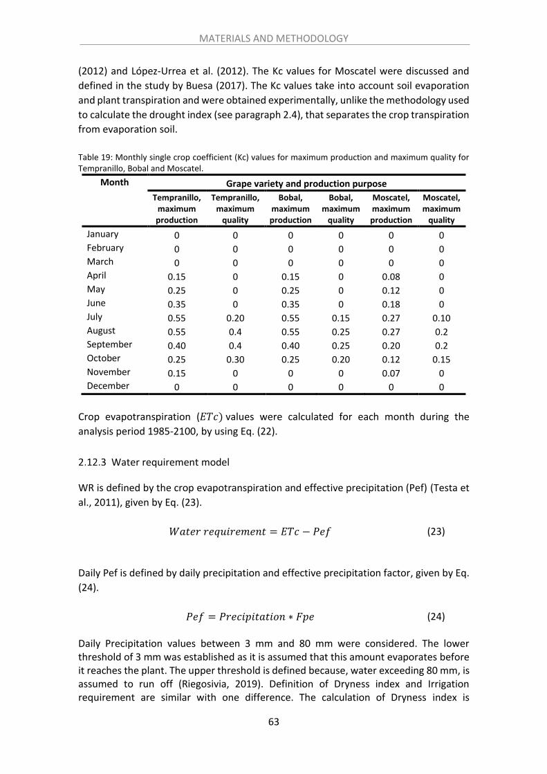
MATERIALS AND METHODOLOGY
63
(2012) and López-Urrea et al. (2012). The Kc values for Moscatel were discussed and
defined in the study by Buesa (2017). The Kc values take into account soil evaporation
and plant transpiration and were obtained experimentally, unlike the methodology used
to calculate the drought index (see paragraph 2.4), that separates the crop transpiration
from evaporation soil.
Table 19: Monthly single crop coefficient (Kc) values for maximum production and maximum quality for Tempranillo, Bobal and Moscatel.
Month Grape variety and production purpose
Tempranillo, maximum production
Tempranillo, maximum
quality
Bobal, maximum production
Bobal, maximum
quality
Moscatel, maximum production
Moscatel, maximum
quality
January 0 0 0 0 0 0 February 0 0 0 0 0 0 March 0 0 0 0 0 0 April 0.15 0 0.15 0 0.08 0 May 0.25 0 0.25 0 0.12 0 June 0.35 0 0.35 0 0.18 0 July 0.55 0.20 0.55 0.15 0.27 0.10 August 0.55 0.4 0.55 0.25 0.27 0.2 September 0.40 0.4 0.40 0.25 0.20 0.2 October 0.25 0.30 0.25 0.20 0.12 0.15 November 0.15 0 0 0 0.07 0 December 0 0 0 0 0 0
Crop evapotranspiration (𝐸𝑇𝑐) values were calculated for each month during the
analysis period 1985-2100, by using Eq. (22).
Water requirement model
WR is defined by the crop evapotranspiration and effective precipitation (Pef) (Testa et
al., 2011), given by Eq. (23).
𝑊𝑎𝑡𝑒𝑟 𝑟𝑒𝑞𝑢𝑖𝑟𝑒𝑚𝑒𝑛𝑡 = 𝐸𝑇𝑐 − 𝑃𝑒𝑓
(23)
Daily Pef is defined by daily precipitation and effective precipitation factor, given by Eq.
(24).
𝑃𝑒𝑓 = 𝑃𝑟𝑒𝑐𝑖𝑝𝑖𝑡𝑎𝑡𝑖𝑜𝑛 ∗ 𝐹𝑝𝑒
(24)
Daily Precipitation values between 3 mm and 80 mm were considered. The lower threshold of 3 mm was established as it is assumed that this amount evaporates before it reaches the plant. The upper threshold is defined because, water exceeding 80 mm, is assumed to run off (Riegosivia, 2019). Definition of Dryness index and Irrigation requirement are similar with one difference. The calculation of Dryness index is

MATERIALS AND METHODOLOGY
64
considered Wo (200 mm) and potential water deficit should not exceed Wo (Tonietto & Carbonneau, 2004). Fpe is defined as two different values during the winter and summer time (see Table 20). Table 20: Effective precipitation factor values (Testa et al., 2011).
Time period Fpe
Winter (from 1.11 to 31.3) 0.75 Summer (from 1.4. to 31.9) 0.25
The monthly necessity of irrigation for two periods were calculated. The first period was
defined from 1985 to 2005 and the second period from 2006 to 2100. The irrigation
scenarios under RCP4.5 and RCP8.5 were calculated for the second period. According to
the time periods, the irrigation necessity models for maximum productivity and
maximum quality were calculated of all three analysed grape varieties. According to
Table 19, values of “0” for single crop coefficient difference between the maximum
quality and maximum production columns, mean there are no irrigation requirements.
Therefore, only the months where the single crop coefficient value is higher than “0”,
were taken into account in the irrigation necessity analysis.
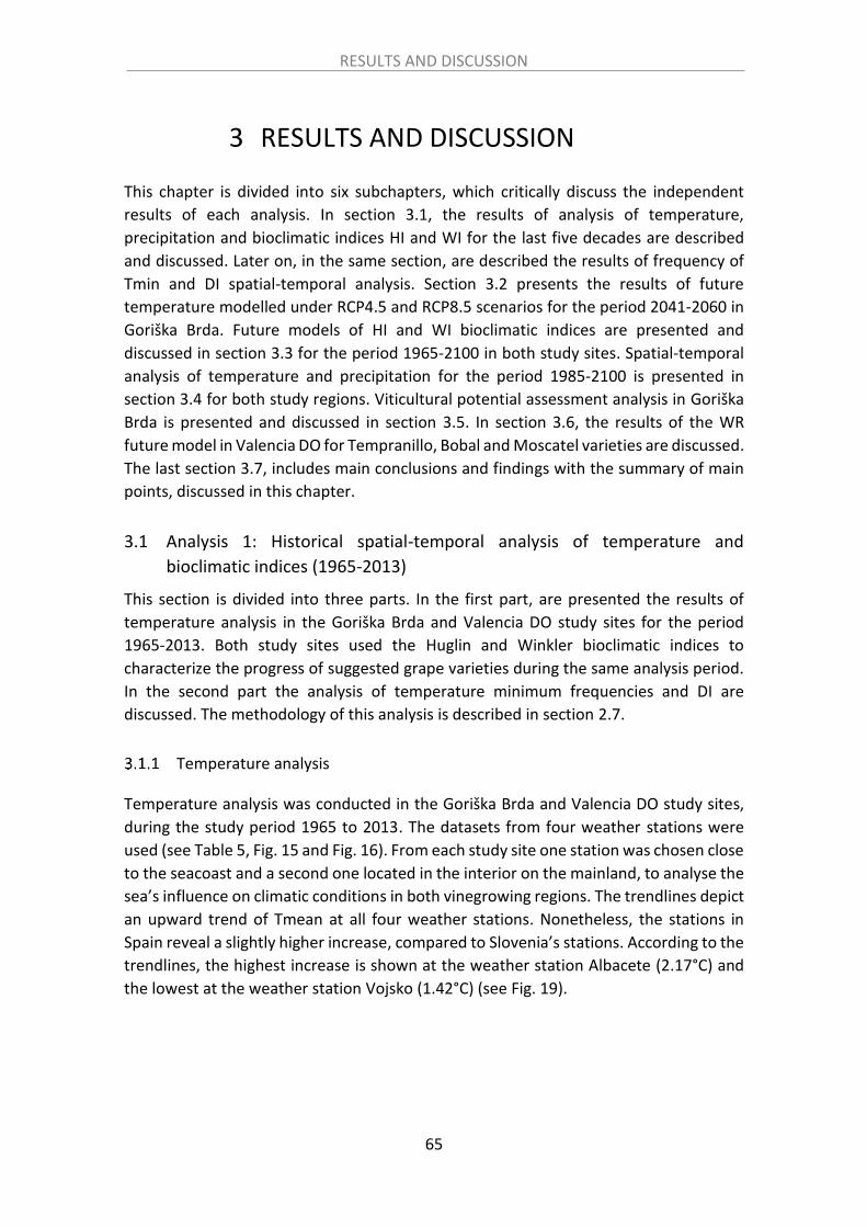
RESULTS AND DISCUSSION
65
3 RESULTS AND DISCUSSION
This chapter is divided into six subchapters, which critically discuss the independent
results of each analysis. In section 3.1, the results of analysis of temperature,
precipitation and bioclimatic indices HI and WI for the last five decades are described
and discussed. Later on, in the same section, are described the results of frequency of
Tmin and DI spatial-temporal analysis. Section 3.2 presents the results of future
temperature modelled under RCP4.5 and RCP8.5 scenarios for the period 2041-2060 in
Goriška Brda. Future models of HI and WI bioclimatic indices are presented and
discussed in section 3.3 for the period 1965-2100 in both study sites. Spatial-temporal
analysis of temperature and precipitation for the period 1985-2100 is presented in
section 3.4 for both study regions. Viticultural potential assessment analysis in Goriška
Brda is presented and discussed in section 3.5. In section 3.6, the results of the WR
future model in Valencia DO for Tempranillo, Bobal and Moscatel varieties are discussed.
The last section 3.7, includes main conclusions and findings with the summary of main
points, discussed in this chapter.
3.1 Analysis 1: Historical spatial-temporal analysis of temperature and
bioclimatic indices (1965-2013)
This section is divided into three parts. In the first part, are presented the results of
temperature analysis in the Goriška Brda and Valencia DO study sites for the period
1965-2013. Both study sites used the Huglin and Winkler bioclimatic indices to
characterize the progress of suggested grape varieties during the same analysis period.
In the second part the analysis of temperature minimum frequencies and DI are
discussed. The methodology of this analysis is described in section 2.7.
Temperature analysis
Temperature analysis was conducted in the Goriška Brda and Valencia DO study sites,
during the study period 1965 to 2013. The datasets from four weather stations were
used (see Table 5, Fig. 15 and Fig. 16). From each study site one station was chosen close
to the seacoast and a second one located in the interior on the mainland, to analyse the
sea’s influence on climatic conditions in both vinegrowing regions. The trendlines depict
an upward trend of Tmean at all four weather stations. Nonetheless, the stations in
Spain reveal a slightly higher increase, compared to Slovenia’s stations. According to the
trendlines, the highest increase is shown at the weather station Albacete (2.17°C) and
the lowest at the weather station Vojsko (1.42°C) (see Fig. 19).

RESULTS AND DISCUSSION
66
Figure 19: Progress of Tmean at all four weather stations during study period. VLC_AIR refers to the weather station Valencia airport. Black straight lines represent temperature trendlines, calculated with linear regression.
Both Spanish weather stations recorded a more intense increase in Tmean, compared
to the Slovene weather stations. The figures show an increase in Tmean at station
Albacete of 2.17°C, which is significantly higher to the increase in temperature at station
Valencia airport (1.59°C), located closer to the coastline. The increase in Tmean during
the research period at Bilje station, was 1.42°C and at Vojsko station, 1.09°C. The
increase difference of Tmin and Tmax at both weather stations is similar (see Table 21).
Table 21: Tmean progress in used weather stations during the study period 1965-2013. VLC_air stands for Valencia airport weather station.
Weather station
Tmean in 1965 (°C)
Tmean in 2013 (°C)
Increase of Tmean trend values 1965-2013 (°C)
VLC_air 16.54 18.13 1.59 Albacete 12.85 15.03 2.17 Bilje 11.61 13.03 1.42 Vojsko 6.01 7.10 1.09
Spanish weather stations also depict a higher increase in Tmin and Tmax, compared to
the Slovene stations. The highest temperature growth shows a Tmin in Valencia DO of
(2.03°C). The lowest increase in average Tmean during the period of research (1.25°C)
was in the Goriška Brda region. The Tmean reveals the highest difference in temperature
growth, comparing both study sites. The average Tmean increase in Valencia DO is
1.88°C and in Goriška Brda 1.25°C (see Fig. 20).
5.0
7.0
9.0
11.0
13.0
15.0
17.0
19.0
21.0
1965 1969 1973 1977 1981 1985 1989 1993 1997 2001 2005 2009 2013
Ave
rage
an
nu
al t
emep
ratu
re (
°C)
Tmean_VLC_AIR Tmean_BILJE
Tmean_Albacete Tmean_Vojsko

RESULTS AND DISCUSSION
67
Figure 20: Average annual increase of mean, minimum and maximum for the period 1965-2013, comparison between Valencia DO and Goriška Brda study site.
Spatial-temporal analysis of bioclimatic indices HI and WI
Bioclimatic indices were calculated from the temperature data, measured at the same
four weather stations used for temperature measurements. Since bioclimatic indexes
are determined from the air temperature measurements, the increase of HI and WI was
expected over the whole study period. The HI progress shows a gradual increase at all
stations during the analysis period. Progress at all four weather stations show steady
growth with notable positive (around 1980, 1888, 1999 and 2011) and negative peaks
(1984, 1995 and 2004). The highest HI increase, according to the trendline, is shown at
the Albacete weather station (479.55 HI points) and the lowest HI increase at the Vojsko
weather station (357.48 HI points) (see Fig. 21).
Figure 21: Fluctuation of HI at the four weather stations during the study period. Black straight lines represent temperature trendlines, calculated with linear regression. HI stands for Huglin index and VLC_AIR refers to weather station Valencia airport.
Classification of HI classes at weather station Albacete shifted from “Warm HI class” to
“Hot HI class” during the study period. Weather station Valencia airport remains in the
“Hot HI class”. Bilje weather station indicates a shift from “Cool HI class” to “Warm HI
class”. The Vojsko weather station remains in the ‘Very cold’ HI class. The Valencia DO
0
0.5
1
1.5
2
2.5
Tmean Tmin Tmax
Ave
rage
an
nu
al
tem
epra
ture
(°C
)
Valencia Brda
500
1000
1500
2000
2500
3000
1965 1969 1973 1977 1981 1985 1989 1993 1997 2001 2005 2009 2013
Hu
glin
po
ints
HI_VLC_AIR HI_BILJEHI_Albacete HI_Vojsko

RESULTS AND DISCUSSION
68
site was ranked two HI classes higher than the Brda study site during the study period.
WI and HI progress during the analysis period show similar trends. Also, WI progress
clearly indicates a positive trend at all weather stations (see Fig. 22).
Figure 22: WI at the four weather stations during the study period. Black straight lines represent temperature trendlines, calculated with linear regression. WI refers to WI and VLC_AIR refers to weather station Valencia airport.
All weather stations clearly show an increase in the WI including notable positive (1982,
1994, 2003) and negative (1972, 1984 and 1996) peaks. The WI progress shows the
lowest value in 1985 at all four weather stations, just one year after the lowest value of
HI progress. The lowest WI increase during the research period, according to the
trendline, is shown at the weather station Vojsko (215.61 WI points) and the highest at
station Albacete (531.36 WI points). The WI growth in Valencia DO (491.85 WI points)
shows a higher increase, compared to Goriška Brda (330.18 WI points). The lower
difference indicates the HI comparison between the two sites. Valencia DO depicts an
increase of 429.32 HI points and Goriška Brda of 388.76 HI points. As seen in the WI and
HI analysis, the Vojsko weather station was the least affected by climate change, in
comparison with the other three weather stations. The highest influence of climate
change was observed at the Albacete weather station. As seen in the WI and HI analysis,
the Vojsko weather station was the least affected by climate change in comparison with
the other three weather stations. The highest influence of climate change was observed
at the Albacete weather station. This shows that climate change has affected the
Valencia site more than the Brda site.
The reason for the lower increase in temperatures at stations closer to the seacoast is
most probably due to the influence of the Mediterranean Sea, which mitigates the
effects of climate change. The Sea’s influence decreases as you move further away from
the seacoast, which can be observed at the weather stations located further away from
the Mediterranean Sea. Nevertheless, the Mediterranean Sea appears to have a minor
influence on Slovenia research site. At the weather station closest to the coastline sea
(Bilje), the mean temperature increase was significantly higher, than the mean
300
800
1300
1800
2300
2800
1965 1968 1971 1974 1977 1980 1983 1986 1989 1992 1995 1998 2001 2004 2007 2010 2013
Win
kler
po
ints
WI_VLC_AIR WI_BILJE
WI_Albacete WI_Vojsko

RESULTS AND DISCUSSION
69
temperatures at weather station Vojsko, located inland. The most likely reason is a
geographical barrier, the hilly part of the region Kras, namely the Trešnik hills (502 m
asl) which lie between weather station Bilje and the Mediterranean Sea, thus preventing
the Sea’s direct influence.
Minimum temperature frequency analysis
In this analysis the ripening season was defined from 1st July to 31st September, as
defined in the study by Bonnardot (2012). From the Goriška Brda site were chosen seven
weather stations (Vogel, Vojsko, Postojna, Godnje, Bilje, Fossalon and Lignano) and, in
the Valencia DO site, nine (Valencia airport, Albacete, Llíria, Castellón, Campo Arcís,
Benifaió, Moncada, Cheste and Teruel) with the required input datasets (see Table 5,
Fig. 15 and Fig. 16). Due to accessible temperature datasets from the meteorological
stations, the frequency of daily Tmin was calculated for the years 2000 and 2016. Two
years were chosen due to a statistical trend between the defined years. In Goriška Brda
(for 2000 and 2016), weather stations closer to the sea, show a higher frequency of the
warmest Tmin (>20°C), especially at stations Fossalon and Lignano. The higher frequency
of coldest Tmin is shown at the weather stations with a lower sea impact, thus those
further from the seacoast and at higher altitudes (Vogel, Vojsko and Postojna). In the
year 2016, at the station Lignano the frequency (from 28% to 62%) of warmest Tmin
(>20°C) more than doubles, compared to the year 2000. Nevertheless, at Fossalon
weather station, the frequency of warmest Tmin diminishes from 49% to 13%. However,
other weather stations show an increase in frequency of warmest Tmin, which suggests
an overall increasing trend. The frequencies of colder Tmin depict a downward trend
from 2000 to 2016 (see Fig. 23).
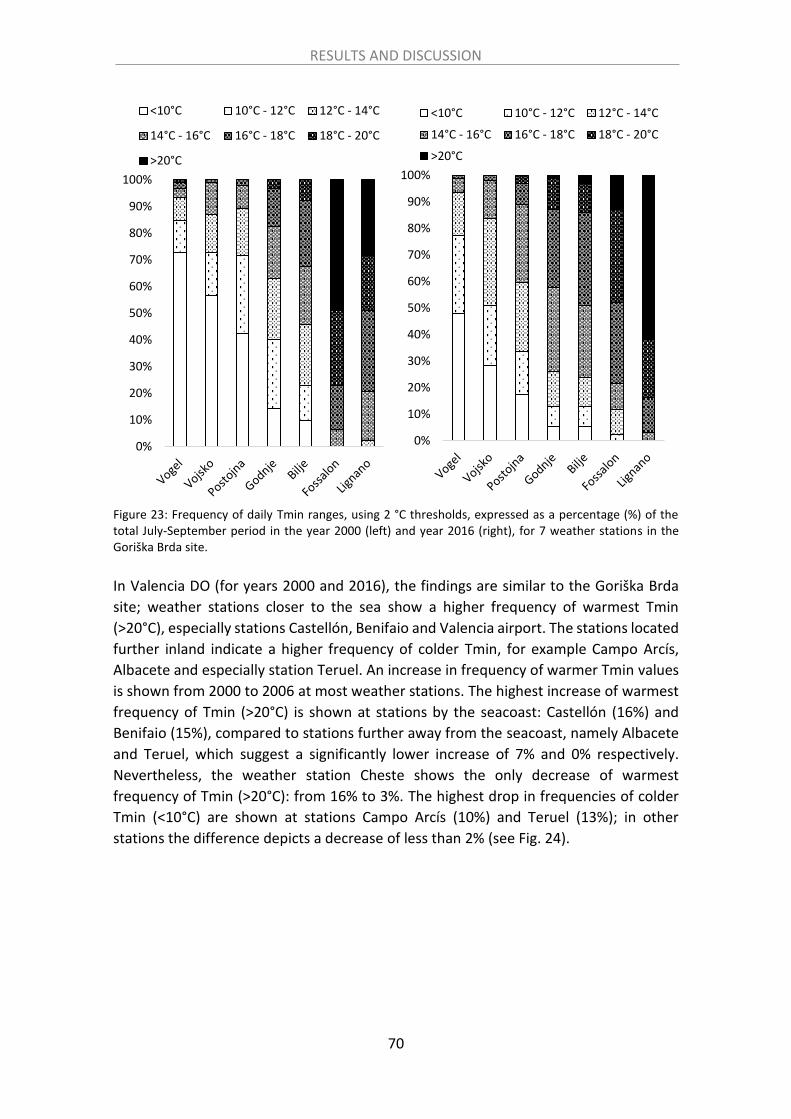
RESULTS AND DISCUSSION
70
Figure 23: Frequency of daily Tmin ranges, using 2 °C thresholds, expressed as a percentage (%) of the total July-September period in the year 2000 (left) and year 2016 (right), for 7 weather stations in the Goriška Brda site.
In Valencia DO (for years 2000 and 2016), the findings are similar to the Goriška Brda
site; weather stations closer to the sea show a higher frequency of warmest Tmin
(>20°C), especially stations Castellón, Benifaio and Valencia airport. The stations located
further inland indicate a higher frequency of colder Tmin, for example Campo Arcís,
Albacete and especially station Teruel. An increase in frequency of warmer Tmin values
is shown from 2000 to 2006 at most weather stations. The highest increase of warmest
frequency of Tmin (>20°C) is shown at stations by the seacoast: Castellón (16%) and
Benifaio (15%), compared to stations further away from the seacoast, namely Albacete
and Teruel, which suggest a significantly lower increase of 7% and 0% respectively.
Nevertheless, the weather station Cheste shows the only decrease of warmest
frequency of Tmin (>20°C): from 16% to 3%. The highest drop in frequencies of colder
Tmin (<10°C) are shown at stations Campo Arcís (10%) and Teruel (13%); in other
stations the difference depicts a decrease of less than 2% (see Fig. 24).
0%
10%
20%
30%
40%
50%
60%
70%
80%
90%
100%
<10°C 10°C - 12°C 12°C - 14°C
14°C - 16°C 16°C - 18°C 18°C - 20°C
>20°C
0%
10%
20%
30%
40%
50%
60%
70%
80%
90%
100%
<10°C 10°C - 12°C 12°C - 14°C
14°C - 16°C 16°C - 18°C 18°C - 20°C
>20°C

RESULTS AND DISCUSSION
71
Figure 24: Frequency of daily Tmin ranges, using 2 °C thresholds, expressed as a percentage (%) of the total July-September period in the year 2000 (left) and year 2016 (right), for 9 available weather station in Valencia DO site.
The highest frequencies of colder Tmin are shown at the Goriška Brda site, compared to
Valencia DO which has a significantly higher frequency of warmer Tmin. Both study sites
indicate a reduction in the frequency of low Tmin from 2000 to 2016 therefore, the
probability of frost events was reduced. According to future warming climate models
(IPCC, 2018), this trend will continue in the future. Generally, the reduction in frequency
of Tmin is similar in both study sites for each year. There is a possibility, that the study
sites experienced an extreme hot or extreme cold year in the chosen analysis years
(2000 and 2016) and therefore, the tendency analysis could be more precise with a
higher number of chosen years.
Temporal analysis of Dryness Index
Goriška Brda and Valencia DO were characterized by dryness parameter DI of the local
climate. The calculations and description of DI are described in the Methodology (see
2.4). The initial useful soil water reserve, which can be accessed by the roots (Wo) was
considered as a value of 200 mm (Tonietto & Carbonneau, 2004). According to the
progress of the DI during the study period (2000-2016), for a majority of the years, the
Goriška Brda site corresponds to the maximum Dryness class DI–2, the “humid” class,
which characterizes humid regions with an absence of dryness. The maximum DI values
0%
10%
20%
30%
40%
50%
60%
70%
80%
90%
100%
<10°C 10°C - 12°C 12°C - 14°C
14°C - 16°C 16°C - 18°C 18°C - 20°C
>20°C
0%
10%
20%
30%
40%
50%
60%
70%
80%
90%
100%
<10°C 10°C - 12°C 12°C - 14°C
14°C - 16°C 16°C - 18°C 18°C - 20°C
>20°C
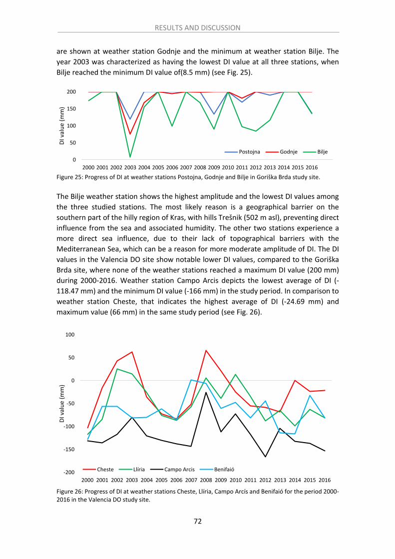
RESULTS AND DISCUSSION
72
are shown at weather station Godnje and the minimum at weather station Bilje. The
year 2003 was characterized as having the lowest DI value at all three stations, when
Bilje reached the minimum DI value of(8.5 mm) (see Fig. 25).
Figure 25: Progress of DI at weather stations Postojna, Godnje and Bilje in Goriška Brda study site.
The Bilje weather station shows the highest amplitude and the lowest DI values among
the three studied stations. The most likely reason is a geographical barrier on the
southern part of the hilly region of Kras, with hills Trešnik (502 m asl), preventing direct
influence from the sea and associated humidity. The other two stations experience a
more direct sea influence, due to their lack of topographical barriers with the
Mediterranean Sea, which can be a reason for more moderate amplitude of DI. The DI
values in the Valencia DO site show notable lower DI values, compared to the Goriška
Brda site, where none of the weather stations reached a maximum DI value (200 mm)
during 2000-2016. Weather station Campo Arcis depicts the lowest average of DI (-
118.47 mm) and the minimum DI value (-166 mm) in the study period. In comparison to
weather station Cheste, that indicates the highest average of DI (-24.69 mm) and
maximum value (66 mm) in the same study period (see Fig. 26).
Figure 26: Progress of DI at weather stations Cheste, Llíria, Campo Arcís and Benifaió for the period 2000-2016 in the Valencia DO study site.
0
50
100
150
200
2000 2001 2002 2003 2004 2005 2006 2007 2008 2009 2010 2011 2012 2013 2014 2015 2016
DI v
alu
e (m
m)
Postojna Godnje Bilje
-200
-150
-100
-50
0
50
100
2000 2001 2002 2003 2004 2005 2006 2007 2008 2009 2010 2011 2012 2013 2014 2015 2016
DI v
alu
e (m
m)
Cheste Llíria Campo Arcis Benifaió

RESULTS AND DISCUSSION
73
Valencia DO also shows an average decrease in DI value of 4.48% during the analysis
period 2000-2016 according to trendline. The average DI class calculated from all four
weather stations, was -65.00 mm, which corresponds to “Moderately dry” DI class. The
Goriška Brda site reveals an increase of 1.11% in DI values during the analysis period and
the average value of DI, characterizes the site as “Humid” class. Amongst both study
sites, the maximum increase is shown at weather station Godnje and the maximum
decrease at weather station Llíria. The average DI value for the period 2000-2016 was
239.47 mm higher in the Goriška Brda site, compared to the Valencia DO site (see Fig.
27).
Figure 27: The increase of DI values in mm at each weather station, according to the trendline for the period 2000-2016 in Goriška Brda (upper map) and Valencia DO (lower map).
The comparison of DI values reveals a significant difference in water conditions between
both sites, which represent distinct effects on viticulture. Precipitation in the Valencia
Do site shows significantly inferior values, compared to the Goriška Brda site (see 2.2),
therefore any kind of lowering of DI values in Valencia DO, would affect viticulture more
than in Goriška Brda. The DI progress during 2000-2016 demonstrates exactly this; a
noticeable decrease of DI in weather stations inside the Valencia DO wine-growing area
(Llíria and Cheste). The closest weather station to the Goriška Brda viticulture region
also showed a negative increase during the analysis period. The classification of classes
did not change during the analysis period in both study sites. Nevertheless, the future
DI tendency in the Valencia DO site, shows a shift to “Very dry” class in the last third of
the 21st century under RCP8.5 scenario, according to the results of the WR analysis (Fig.
66). Every 5-6 years, the Valencia DO site experiences a dry period (Monterde et al.,
2017). According to future climate projections, the period between dry periods will get
shorter in the future (IPCC, 2018). Therefore, the study of dryness index and its tendency
is important in predicting future dry seasons and to enhance the quality and quantity of
the yield.

RESULTS AND DISCUSSION
74
3.2 Analysis 2: Future temperature modelling in the Goriška Brda study site
(2041-2060)
This chapter describes the results of future temperature modelling in the Goriška Brda
viticultural region, using three meteorological stations. The purpose of this research is
to provide a critical analysis of temperature trend for the period 2041-2060, analyse the
influence of the Mediterranean Sea and to conduct comparative statistical analysis
between the results. The methodology used is described in the Methodology chapter
(see 2.8.). Data were retrieved from three weather stations (Vojsko, Bilje and Vedrijan)
distributed inside, and in surroundings of, the wine region Goriška Brda. The future
temperature dataset was retrieved from Worldclim (CMIP5) for two periods (1950-2000
and 2041-2060) under RCP4.5 and RCP8.5 scenarios.
Future temperature model for period 2041-2060
The monthly Tmean shows distinct temperature values, calculated from all three
stations, for the periods 1961-2000 and 2041-2060. In the graph are the following
temperature types: observed temperature for the period 1961-2000, Worldclim
temperature for the period 1950-2000 (reference period) and future simulation under
RCP4.5 and RCP8.5 scenarios. The observed annual Tmean for the period 1961-2000
shows a 0.2°C higher value, compared to the modelized data for the period 1950-2000.
The difference between future modelized (2041-2060) and observed temperatures
(1961-2000) indicates a notable gap. Average annual future modelized Tmean values of
1.7°C and 2.0°C, under RCP4.5 and RCP8.5, respectively, are higher, compared to
observed annual average of Tmean (see Fig. 28).

RESULTS AND DISCUSSION
75
Figure 28: Comparison of monthly average observed and modelized temperature. The observation data were obtained from monthly temperature averages from weather stations Bilje, Vojsko and Vedrijan.
The temperatures reveal the hottest month is July and the coldest January. The
observed and modelized mean temperatures for the period 1950-2000 demonstrate
significantly lower values, compared to the modelized temperatures for the period
2041-2060. Furthermore, temperatures under RCP8.5, indicate notably higher values,
compared to RCP4.5 scenario. Future temperatures under RCP8.5 were expected to be
higher than RCP4.5, due to nature of climate scenarios (Van Vuuren et al., 2011).
November shows the highest rise from observed temperatures (reference period) to
future, under RCP8.5 scenario (2.6°C). However, the lowest rise shows April under
RCP4.5 (1.1°C). Temperature values between Tmax and Tmin show dissimilarities at all
three weather stations for the period 1961-2000 (see Fig. 29).
0
5
10
15
20JA
NU
AR
Y
FE
BR
UA
RY
MA
RC
H
AP
RIL
MA
Y
JUN
E
JUL
Y
AU
GU
ST
SE
PT
EM
BE
R
OC
TO
BE
R
NO
VE
MB
ER
DE
CE
MB
ER
An
nu
al T
mea
n(°
C)
Tmean_observed (1961-2000)
Tmean_modelized (1950-2000)
Tmean_modelized_RCP4.5 (2041-2060)
Tmean_modelized_RCP8.5 (2041-2060)

RESULTS AND DISCUSSION
76
Figure 29: Comparison of average observed (time period 1961-2000) and average modelized (time period 2041-2060) minimum (Tmin) and maximum (Tmax) temperature at weather stations Bilje, Vojsko and Vedrijan.
Bilje, the closest weather station to the Mediterranean Sea, indicates the highest
average Tmax (20.1°C) for the period 2041-2060 (under RCP8.5 scenario). It also shows
the highest difference (Tmin) between observed and modelized data for the period
1950-2000: 2.5°C. One of the most probable reasons for the notable difference between
modelized and observed temperature for the period 1950-2000, is the spatial resolution
of climatic model. Observation data were gathered from three exact points, namely the
locations of the three weather stations (Bilje, Vojsko and Vedrijan). In contrast, the
Worldclim data were generated through the interpolation of average monthly data from
weather stations on a 30 arc-second resolution grid. Due to interpolation from several
weather stations, the accuracy of Worldclim data is not as high as on directly observation
data from weather stations. The other reason for the difference between observed and
Worldclim data, is the period during which the observation data was retrieved. For
optimum results, the datasets from the period 1950-2000 should have been used.
According to available datasets, the stations were chosen due to their availability of data
and closeness to the Goriška Brda site. At weather stations Vojsko and Vedrijan, daily
Tmin and Tmax data were available for the period 1961-2000 and used for the purpose
of this research. The timeframe of used data for Worldclim was 1950-2000, therefore
11 years more data in comparison with weather stations Vojsko and Vedrijan.
Furthermore, the period of data at weather station Vedrijan was from 1960-1990, so 20
years shorter than that used for Worldclim data. The modelized annual average
maximum and Tmin, according to RCP4.5 scenario modelling (for the period 2041-2060)
indicate higher values, compared to observation data for all three weather stations.
0
5
10
15
20
Bilje Vojsko Vedrijan
An
nu
em T
mea
n (
°C)
Observed average Tmax (1961-2000)
Average Tmax modelized data (1961-2000)
Modelized Tmax, RCP4.5 (2041-2060)
Modelized Tmax, RCP8.5 (2041-2060)
Observed average Tmin (1961-2000)
Average Tmin modelized data (1961-2000)
Modelized Tmin, RCP4.5 (2041-2060)
Modelized Tmin, RCP8.5 (2041-2060)

RESULTS AND DISCUSSION
77
However, under RCP8.5 scenario, only at weather stations Vojsko and Vedrijan are
modelized temperatures higher than observed temperatures. The only exception is
weather station Bilje, where the simulation of annual average Tmin, according to RCP8.5
modelling, shows a lower temperature (0.1°C), than the observed annual Tmin at the
same station. The most significant difference in Tmin (2.4°C) between observed (1950-
2000) and modelized (2051-2060) is at stations Vedrijan and Bilje. The lowest increase
in Tmin (1.7°C) under RCP4.5, is shown across all stations (see Table 22).
Table 22: Average annual temperature increase for each weather station under RCP4.5 and RCP8.5 scenarios. Comparing the future period 2041-2060 to reference period 1950-2000.
Increase from 1950-2000 to 2041-2060 Weather stations
Bilje Vojsko Vedrijan
Tmin under RCP8.5 2.4°C 2°C 2.4°C Tmax under RCP8.5 2.2°C 2.2°C 2.2°C Tmin under RCP4.5 1.8°C 1.8°C 1.8°C Tmax under RCP4.5 1.7°C 1.7°C 1.7°C
The temperature increase obtained by comparing the future period 2041-2060 to the
reference period 1950-2000, is the same across all weather stations, with the exception
of the Tmin increase under RCP8.5. Bilje and Vedrijan stations show a 0.4°C higher
increase, compared to Vojsko. The stations closer to the sea indicate a slightly higher
temperature increase in the future. Between the Mediterranean Sea and weather
station Bilje, there is a natural barrier, the hilly part of the region Kras, (highest hill
Trešnik (502 m asl) reduces most of the Sea’s direct influence. However, the weather
station Bilje lies in a river valley (river Vipava), which runs around the hilly site and joins
the river Soča, that flows into the Mediterranean Sea. Consequently, the influence of
the sea is present through both river valleys and it influences the local climate on
weather station Bilje. According to the topography, weather station Bilje has the most
indirect influence of the Mediterranean Sea among the three weather stations. Weather
stations Vedrijan and Vojsko lie at approximately double the distance from the seacoast,
in comparison with weather station Bilje. Vojsko weather station experiences the most
direct sea influence and Vedrijan the least. Therefore, the sea influence on temperature
increase, as a water mass to moderate the influence of climate change, demonstrates a
roughly similar impact on all three weather stations. Nevertheless, the stations lie very
short distances apart. The maximum air distance of 25km is between Vojsko and Bilje.
Overall, Goriška Brda region, according to Vedrijan station, located inside of the region,
is expected to experience a temperature increase of between 1.8°C and 1.7°C under
RCP4.5 and RCP8.5 scenarios respectively, until period 2041-2060 (compared to the
reference period 1961-2000).

RESULTS AND DISCUSSION
78
3.3 Analysis 3: Spatial-temporal analysis of temperature and bioclimatic indices
(1965-2100)
The objective of this analysis was to conduct a critical analysis of temperature and bioclimatic indices Huglin and Winkler under RCP4.5 and RCP8.5 scenarios during the period 1965-2100 in both study sites. This chapter is divided into two sections: In the first section are presented results and discussion from the study site Goriška Brda, and in the second, are presented results and discussion from the study site Valencia DO. The methodology is described in the Methodology chapter (see 2.9.).
Temperature and bioclimatic indices temporal analysis in Goriška Brda (1965-
2100)
For the purpose of temperature and bioclimatic analysis, the average temperature data from three weather stations in Goriška Brda were chosen: Godnje, Vojsko and Bilje (see Table 5 and Fig. 15). The stations which were closest to Goriška Brda and that had the longest daily temperature observation history were chosen. In this analysis were used observation datasets of daily Tmean for the period 1965-2016, and Tmean datasets for the period 1985-2100 under RCP4.5 and RCP8.5 scenarios, retrieved from the Euro-Cordex dataset (Jacob et al., 2014). The progress of annual Tmean shows an upward trend during the entire period (1965-2100) (see Fig. 30).
Figure 30: Temperature analysis of average values of the three weather stations Vojsko, Godnje and Bilje.
Tmean observations stands for average annual observation data from 1965-2016, Tmean_rcp45 stands
for average annual modelized temperature under RCP4.5 scenario (2005-2100) and Tmean_rcp85 stands
for average annual modelized temperature under RCP8.5 scenario (2005-2100).
The difference in temperature progress under RCP4.5 and RCP8.5 scenarios is insignificant until the year 2050. After 2050, the difference increases, especially in temperature progress under RCP8.5 scenario. Temperature increase of observation period is 1.77°C, calculated from tendency line with the coefficient of determination of 0.52. During the period 1985-2100, the increment for RCP4.5 scenario shows 2.2°C under RCP4.5 and 4.5°C under RCP8.5 scenario, also calculated from the tendency line. Coefficient of determination for temperature progress under RCP4.5 scenario is 0.84
8
9
10
11
12
13
14
15
16
19
65
19
70
19
75
19
80
19
85
19
90
19
95
20
00
20
05
20
10
20
15
20
20
20
25
20
30
20
35
20
40
20
45
20
50
20
55
20
60
20
65
20
70
20
75
20
80
20
85
20
90
20
95
21
00
An
nu
al m
ean
tem
per
atu
re (
°C)
Tmean_observations
Tmean_RCP4.5
Tmean_RCP8.5

RESULTS AND DISCUSSION
79
and, for temperature progress under RCP8.5 scenario is 0.93. Temperature increase under RCP8.5 scenario indicates a more significant positive trend, compared to RCP4.5 scenario, also discussed in previous research (Van Vuuren et al., 2011). The mean annual observation data were compared with modelized data scenarios RCP4.5 and RCP8.5 to obtain the strength of the correlation between both scenarios. The comparison analysis of observed and modelized annual Tmean shows a common increasing tendency during the period 1985-2016. The RCP’s modelized Tmean line is much smoother, in comparation with observed Tmean line, showing several significant peaks (see Fig. 31).
Figure 31: Left graph: Comparison of observed and modelized annual Tmean under RCP4.5 scenario (1985-2016). Tmean_observations stand for average annual observation temperature from 1985 to 2016 and Tmean_rcp45 stands for average annual modelized temperature under RCP4.5 scenario. Right graph: Comparison of observed and modelized annual Tmean under RCP8.5 scenario (1985-2016). Tmean_observations stand for average annual observation temperature from 1985 to 2016 and T-mean_rcp85 stands for average annual modelized temperature under RCP8.5 scenario.
Average absolute difference between observed and modelized Tmean under RCP4.5 scenario is 0.86°C and is 0.90°C between observed Tmean and temperature under RCP8.5 scenario. Temperature anomaly was calculated for the period 1965-2016 using reference period 1965-1994. Tendency of temperature anomaly depicts steady increase and shows the increment of 1.74°C, according to linear regression with the coefficient of determination 0.49. The trendline reveals negative values until the year 1979, roughly estimated, when the values of the trendline changed into positive values until the year 2016. There were only two negative temperature anomalies after the years 1990; 1996 and 2005. During the period 1965-1990, there were 12 years with a negative temperature anomaly (see Fig. 32).
9
9.5
10
10.5
11
11.5
12
12.5
19
85
19
88
19
91
19
94
19
97
20
00
20
03
20
06
20
09
20
12
20
16
An
nu
al m
ean
tem
per
atu
re (
°C)
Tmean_observations
Tmean_rcp45
9
9.5
10
10.5
11
11.5
12
12.5
19
85
19
88
19
91
19
94
19
97
20
00
20
03
20
06
20
09
20
12
20
16
An
nu
al m
ean
tem
per
atu
re (
°C)
Tmean_observations
Tmean_rcp85

RESULTS AND DISCUSSION
80
Figure 32: Annual Tmean anomaly for period 1965-2016 (observation period). Reference value is 1965-1992. T_anomaly_obs stands for observed annual Tmean. Trendline was calculated with linear regression.
The temperature anomaly under RCP4.5 and RCP8.5 scenarios also indicates a positive trend during analysis for the period 1965-2100. Average annual anomaly shows an increase of 4.12°C (RCP4.5) and 6.29°C (RCP8.5) during the period 1965-2100. Temperature rise was calculated from the trendline, using observation data from 1965-2016 and under RCP4.5 and RCP8.5 scenarios from 2016 to 2100 (see Fig. 33).
Figure 33: Average annual temperature anomaly for the period 1965-2100 for RCP4.5 and RCP8.5 scenarios. T_anomaly_45 stands for temperature anomaly for observation period 1965-2016 and modelized period 2016-2100 according to RCP4.5 scenario and T_anomaly_85 stands for temperature anomaly for observation period 1965-2016 and modelized period 2016-2100 according to RCP8.5 scenario. Solid line presents the 10 years average value. Reference value is the period 1965-1994.
Observation temperature data and modelized scenarios demonstrate an upward trend during the entire analysis period (1965-2100). From the year 2016 until 2039, roughly estimated, the temperature progress under RCP4.5 and RCP8.5 scenarios shows a similar growing pattern. After the year 2040, the Tmean anomaly of both RCP scenarios starts to diverge; temperature anomaly under RCP8.5 scenario begins to rise above the RCP4.5 scenario. The difference grows until the year 2100, where it reaches 2.17°C,
-1.5
-1
-0.5
0
0.5
1
1.5
2
2.5
19
65
19
68
19
71
19
74
19
77
19
80
19
83
19
86
19
89
19
92
19
95
19
98
20
01
20
04
20
07
20
10
20
13
20
16
An
nu
al T
mea
n (
°C)
T_anomaly_obs Trendline
-2
-1
0
1
2
3
4
5
6
19
65
19
70
19
75
19
80
19
85
19
90
19
95
20
00
20
05
20
10
20
15
20
20
20
25
20
30
20
35
20
40
20
45
20
50
20
55
20
60
20
65
20
70
20
75
20
80
20
85
20
90
20
95
21
00
An
nu
al m
ean
tem
per
atu
re (
°C) T_anomaly_45
T_anomaly_85

RESULTS AND DISCUSSION
81
calculated from the tendency line. Coefficient of determination for temperature anomaly is 0.87 under RCP4.5 and 0.95 under RCP8.5 scenario. Both future scenarios show a different temperature increase in the period 1965-2100. The temperature increment indicates significantly superior values under RCP8.5, compared to RCP4.5 scenario. The temperature increase under RCP8.5 shows a higher temperature of 1.78°C, compared to RCP4.5 scenario (see Table 23). Table 23: Increase of Tmean under RCP4.5 and RCP8.5 scenarios under projected period 2071-2100 (period B) compared to the reference period 1965-1992 (period A).
Period Climate scenario
Tmean_RCP4.5 Tmean_RCP8.5
Period A: 1965-1994 9.67°C 9.67°C
Period B: 2071-2100 12.87°C 14.65°C Temperature increase from period A to period B 3.21°C 4.99°C
Progress of observed and modelized HI shows a positive tendency during the entire analysis period 1965-2100. Observed HI during the period 1965-2000 depicts moderate increase and afterwards the tendency slightly escalates during the second observation period 1998-2016 (see Fig. 34).
Figure 34: Progress of observed (1965-2016) and modelized (1985-2100) bioclimatic index Huglin under RCP4.5 and RCP8.5 scenarios. HI_observations stands for annual average value of HI derived from observed temperature during period 1965-2016, HI_RCP4.5 stands for annual average value of HI derived from modelized daily temperature under RCP4.5 scenario 1985-2100 and HI_RCP8.5 stands for annual average value of HI derived from modelized daily temperature under RCP8.5 scenario (1985-2100).
The tendency of modelized HI progress under RCP4.5 and RCP8.5 scenarios also indicates a growing trend during the reference period (1985-2005) and the modelized period (2005-2100). Roughly estimated, the difference in the HI under both climate scenarios considerably diverges from the year 2064. The HI progress under RCP8.5 scenario escalates during the period 2064-2100, compared to the HI progress under RCP4.5 scenario, which shows a moderate and steady increase during the whole
1500
1700
1900
2100
2300
2500
2700
19
65
19
70
19
75
19
80
19
85
19
90
19
95
20
00
20
05
20
10
20
15
20
20
20
25
20
30
20
35
20
40
20
45
20
50
20
55
20
60
20
65
20
70
20
75
20
80
20
85
20
90
20
95
21
00
An
nu
al s
um
of
Hu
glin
po
ints
Hot Warm
Cool Cold
HI_observations HI_RCP4.5
HI_RCP8.5

RESULTS AND DISCUSSION
82
scenario period 2005-2100. Progress of WI also shows a steady increase during the observation and modelized periods. Observed WI during the years 1965-2000 indicates moderate increase and, in continuation, the tendency slightly escalates during the period 2000-2016 (see Fig. 35).
Figure 35: Progress of observed (1965-2016) and modelized (1985-2100) bioclimatic index Winkler under
RCP4.5 and RCP8.5 scenarios. WI_observations stands for annual average value of WI derived from
observed temperature during period 1965-2016, WI_RCP4.5 stands for annual average value of WI
derived from modelized daily temperature under RCP4.5 scenario (1985-2100) and WI_RCP8.5 stands for
annual average value of WI derived from modelized daily temperature under RCP8.5 scenario (1985-
2100).
WI progress under both scenarios shows a steady upward trend during the analysis
period 1985-2100. The difference between the WI progress under both scenarios
indicates a similar trend, however, from the year 2058, roughly estimated, the WI values
under RCP8.5 do start to rise above RCP4.5. The WI progress under RCP8.5 scenario
shows higher growth during the period 2058-2100, compared to RCP4.5 scenario, which
depicts a moderate and steady increase during the whole period 2005-2100. The
increment of both bioclimatic indices shows higher values under RCP8.5 scenarios
during the entire analysis period 1965-2100. WI progress shows the highest increase
under RCP8.5 scenario, 872.52 points. The increase of HI under RCP4.5 scenario,
demonstrates the lowest growth (435.05 points) (see Table 24).
900
1100
1300
1500
1700
1900
2100
2300
19
65
19
70
19
75
19
80
19
85
19
90
19
95
20
00
20
05
20
10
20
15
20
20
20
25
20
30
20
35
20
40
20
45
20
50
20
55
20
60
20
65
20
70
20
75
20
80
20
85
20
90
20
95
21
00
An
nu
al s
um
of
Win
kler
po
ints
Region_4 Region_3
Region_2 Region_1
WI_observatinos WI_RCP4.5
WI_RCP8.5

RESULTS AND DISCUSSION
83
Table 24: Increase of bioclimatic indices Huglin and Winkler in the period 1965-2100 under RCP4.5 and RCP8.5 scenarios. The increase was calculated by increase between reference period 1965-1994 (observation data) and 2071-2100 (modelized scenarios RCP4.5 and RCP8.5).
Time period Bioclimatic index
Huglin, RCP4.5
Huglin, RCP8.5
Winkler, RCP4.5
Winkler, RCP8.5
Period A: 1965-1994 1738.37 1738.37 1219.62 1219.62
Period B: 2071-2100 2173.43 2522.27 1707.45 2081.72
Bioclimatic index increase from period A to period B
435.05 783.89 487.83 862.10
In the year 1965, viticultural site Brda was classified as HI’s “Cold class” and WI‘s “First region”. Hence, the suggested grape varieties according to bioclimatic index WI are Pinot noir, Riesling, Chardonnay, Gewurztraminer, Pinot grigio; according to HI: Sauvignon blanc, Riesling, Pinot noir, Chardonnay, Merlot and Cabernet franc. The common grape varieties, which are stated in HI ‘s “Cold class” and in “First region” of WI class, are Chardonnay and Riesling. By the year 2016, HI shifted to the next class, “Cool class” and WI to the next region, “Second region”. Proposed grape varieties for Cool HI class are: Cabernet Sauvignon, Ugni Blanc and Syrah. Suggested grape varieties for WI second region are: Cabernet sauvignon, Chardonnay, Merlot, Semillon and Syrah. Common grape varieties for both bioclimatic indices are Cabernet sauvignon and Syrah. The most important grape varieties for Goriška Brda in 2016 were Rebula (Ribolla Gialla), Chardonnay, Merlot, Sauvignonasse (Tocai Friulano) and Sivi pinot (Pinot gris) (Gorjak, 2017). In comparison to the recommended varieties, there are two varieties in common. Chardonnay variety is suggested by both bioclimatic indices. Merlot is recommended by HI and is also a recommended variety in Goriška Brda according to Slovene viticulture legislation (Legal Information System of Slovenia, 2019). According to RCP4.5 scenario, the HI class for Goriška Brda will shift until the year 2100
to “Warm class” with recommended grape varieties: Grenache, Mourvèdre and
Carignan. WI will shift to the next region, “Third region”, with recommended varieties:
Grenache, Barbera, Tempranillo and Syrah. Variety Granache is the only grape variety in
common. According to RCP8.5 scenario there will be even more considerable shifts in
bioclimatic classes. HI class will shift until the year 2100 by two classes. Goriška Brda will
be in HI’s “Hot class”, which exceeds the heliothermic necessity to ripen the varieties,
even the late ones. WI will shift until the year 2100 to the “Fourth region” with suggested
grape varieties: Carignan, Cinsault, Mourvedre and Tempranillo. Goriška Brda will reach
the penultimate class in both bioclimatic indices under RCP8.5 future climate scenario.
The temperature increase during the period 2061-2100 of this section was compared to
the temperature growth in section 3.2 in the same study site. The results from this
analysis reveal a higher temperature increment under RCP4.5 and RCP8.5 scenarios. The
temperature increases are higher by 0.81°C and 0.85°C, under RCP4.5 and RCP8.5
respectively (see Table 25).

RESULTS AND DISCUSSION
84
Table 25: Temperature increase from baseline (T1) to period T2. Baseline is defined as 1961-2000 (Worldclim) and 1963-1992 (Euro-Cordex). T2 is defined from 2041-2060.
Section 3.2. (Worldclim dataset)
Section 3.3.1 (Euro-Cordex dataset)
RCP4.5 RCP8.5 RCP4.5 RCP8.5
Temperature increase from period T1 to T2 (°C) 1.75 2.23 2.56 3.08
The differences between the results were caused due to several possible reasons. (a) In
section 3.2 the Worldclim dataset was used with distinct spatial resolution (approx. 1
km x 1 km), compared to the resolution with the Euro-Cordex dataset (approx. 12.5 km
x 12.5 km). Furthermore, the methodology for elaborating each climate model is distinct
(Hijmans et al., 2005; Jacob et al., 2014). (b) In section 3.2 a different baseline (1961-
2000) was adopted, compared to 1963-1992, due to obtainable observation data. (c) In
the section 3.2 were also used three weather stations, however the station Vedrijan was
replaced by Godnje in this section, due to availability of observation data. Probably the
most likely reason for the different temperature increases was caused by the usage of
distinct climate models with a different spatial resolution.
Temperature and bioclimatic indices temporal analysis in Valencia DO (1965-
2100)
According to available historical daily temperature data, tone weather station was
chosen for this analysis in the Valencia DO site: Valencia airport (see Table 5 and Fig. 16).
The analysis period 1965-2100 was chosen, under forcing scenarios RCP4.5 and RCP8.5
(see 3.3.1). Temperature progress shows a steady increase at both stations during the
period 1965-2100. Temperatures observations indicate a slightly decreasing tendency
until the year 1972 and, afterwards, a steady increase until the year 2016. The observed
temperatures reveal mostly higher values, compared to the modelized temperatures,
during the observation period (1985-2016). The modelized temperature progress
depicts a steady, positive trend during 1985-2100 under both scenarios. The
temperatures under RCP4.5 and RCP8.5 scenarios show a similar fluctuation until the
year 2050. Afterwards, the models diverge and temperature progression under RCP8.5
demonstrates an increasing positive difference until 2100 in contrast with the
temperature development under RCP4.5, which indicates a significantly moderate
tendency after 2050 (see Fig. 36).

RESULTS AND DISCUSSION
85
Figure 36: Temperature analysis of average values of the weather station Valencia airport. Tmean_observations stands for average annual observation data from 1965-2016, Tmean_RCP4.5 stands for average annual modelized temperature under RCP4.5 scenario (2005-2100) and Tmean_RCP85 stands for average annual modelized temperature under RCP8.5 scenario (2005-2100).
Temperature progress of observed and modelized temperatures show a noticeable
difference during the period 1985-2016 (Fig. 37). Both temperature advances depict a
similar growing tendency, however, observed temperatures indicate higher values
during the observation period, compared to modelized temperatures. This is in contrast
with temperature progress in the Goriška Brda site, where observed temperatures
indicate mostly lower values compared to modelized temperatures. The absolute
average difference between observed and modelized temperature progress is 0.52°C
(RCP4.5 and RCP8.5).
Figure 37: Left graph: Comparison of observed and modelized annual Tmean, scenario RCP4.5 in the period 1985-2016. Tmean_observations stands for average annual observation temperature from 1985 to 2016 and T_mean_rcp45 stands for average annual modelized temperature under RCP4.5 scenario. Right graph: Comparison of observed and modelized annual Tmean under RCP8.5 in the period 1985-2016. Tmean_observations stand for average annual observation temperature from 1985 to 2016 and T_mean_rcp85 stands for average annual modelized temperature under RCP8.5 scenario.
15
16
17
18
19
20
21
22
19
65
19
70
19
75
19
80
19
85
19
90
19
95
20
00
20
05
20
10
20
15
20
20
20
25
20
30
20
35
20
40
20
45
20
50
20
55
20
60
20
65
20
70
20
75
20
80
20
85
20
90
20
95
21
00
An
nu
al m
ean
tem
per
atu
re (
°C)
Tmean_observations
Tmean_RCP4.5
Tmean_RCP8.5
16
17
18
19
20
21
22
19
85
19
88
19
91
19
94
19
97
20
00
20
03
20
06
20
09
20
12
20
16
An
nu
al m
ean
tem
per
atu
re (
°C)
Tmean_observations
Tmean_rcp45
16
17
18
19
20
21
22
19
85
19
88
19
91
19
94
19
97
20
00
20
03
20
06
20
09
20
12
20
16
An
nu
al m
ean
tem
per
atu
re (
°C) Tmean_observations
Tmean_rcp85

RESULTS AND DISCUSSION
86
The progress of temperature anomaly of observation data demonstrates a slightly
negative tendency until the year 1976 and, afterwards, an increased positive tendency
until 2016. According to the trendline, calculated with linear regression, temperature
anomaly reveals a general positive tendency during observation period 1965-2016.
Deviation from trendline show higher values during the second half of the whole analysis
period. The temperature anomaly increases by 1.72°C, according to the trendline (1965-
2016) with the coefficient of determination 0.43. The increase is 0.02°C lower, compared
to the Goriška Brda site (see Fig. 32). The trendline tendency shows a similar trend as
the one for the Goriška Brda site. The point of crossing the 0°C axis occurs 3 years later
(1978), compared to the Goriška Brda (see Fig. 38).
Figure 38: Annual Tmean anomaly for period 1965-2016 (observation period). Reference value was 1965-1994. T_anomaly_obs stands for observed annual Tmean. Trendline was calculated with linear regression.
The temperature anomaly of observations demonstrates a negative tendency until the
year 1985, roughly estimated. Afterwards, both models indicate a positive tendency
until 2100. The modelized temperatures under both scenarios show similar upward
trends, roughly until 2043: thereafter the anomalies under RCP4.5 and RCP8.5 scenarios
diverge. The temperature anomaly under RCP8.5 scenario depicts a significantly higher
increase, compared to the temperature anomaly under RCP4.5 scenario. Analysis of the
Goriška Brda site shows fewer and less intense negative values of temperature anomaly,
compared to the Valencia DO site. Nevertheless, most of the negative values were
noticed in similar periods in both study sites: 1968-2018, roughly estimated (see Fig. 39).
-1.5
-1
-0.5
0
0.5
1
1.5
2
2.5
19
65
19
68
19
71
19
74
19
77
19
80
19
83
19
86
19
89
19
92
19
95
19
98
20
01
20
04
20
07
20
10
20
13
20
16
An
nu
al m
ean
tem
per
atu
re (
°C)
T_anomaly_obs
Trendline

RESULTS AND DISCUSSION
87
Figure 39: Average annual temperature anomaly for the period 1965-2100 for RCP4.5 and RCP8.5 scenarios. T_anomaly_45 stands for temperature anomaly for observation period 1965-2016 and modelized period 2016-2100 according to RCP4.5 scenario and T_anomaly_85 stands for temperature anomaly for observation period 1965-2016 and modelized period 2016-2100 according to RCP8.5 scenario. Solid lines present the 10 years average value. Reference value is the period 1965-1994.
Temperature growth suggests a different increment between both RCP scenarios. A
higher increase, according to the reference period 1965-1994, indicates a temperature
fluctuation under RCP8.5 scenario of 3.82°C. The increase under RCP4.5 scenario shows
a significantly inferior value: 2.07°C, which is 1.75°C lower, compared to the RCP8.5
scenario (see Table 26).
Table 26: Increase of Tmean under RCP4.5 and RCP8.5 scenarios under projected period 2071-2100, compared to the reference period 1965-1994.
Period Climate scenario
Tmean_RCP4.5 Tmean_RCP8.5
Period A: 1965-1994 16.98°C 16.98°C
Period B: 2071-2100 19.05°C 20.80°C Temperature increase from period A to period B 2.07°C 3.82°C
The HI progress indicates a steady positive tendency during the whole analysis period
(1965-2100), with the exception of observation period 1965-1977, where HI tendency
shows negative values. Observation and modelized progress of HI during the period
1985-2016 indicate a difference, however, the tendencies of both progressions reveal a
similar trend. The modelized HI progress depicts similar steady progress under both RCP
scenarios until 2050, roughly estimated, when the progress is diverged. HI under RCP4.5
scenario continues a steady, positive tendency until 2100. In contrast, the HI progress
under RCP8.5 reveals a higher increase and escalation until 2100, compared to RCP4.5
scenario (see Fig. 40).
-2
-1
0
1
2
3
4
5
19
65
19
70
19
75
19
80
19
85
19
90
19
95
20
00
20
05
20
10
20
15
20
20
20
25
20
30
20
35
20
40
20
45
20
50
20
55
20
60
20
65
20
70
20
75
20
80
20
85
20
90
20
95
21
00
An
nu
al m
ean
tem
per
atu
re (
°C)
T_anomaly_45
T_anomaly_85

RESULTS AND DISCUSSION
88
Figure 40: Progress of observed (1965-2016) and modelized (1985-2100) bioclimatic index Huglin under RCP4.5 and RCP8.5 scenarios. HI_observations stands for annual average value of HI derived from observed temperature during period (1965-2016), HI_rcp4.5 stands for annual average value of HI derived from modelized daily temperature under RCP4.5 scenario (1985-2100) and HI_rcp8.5 stands for annual average value of HI derived from modelized daily temperature under RCP8.5 scenario (1985-2100).
Similarly, the progress of WI shows a steady increase during the analysis period (1965-
2100), with the exception of period 1965-1977, where the progress tendency indicates
negative values. Observation and modelized progress of WI during the period 1985-2016
demonstrate different values, however, the tendencies of both progressions are similar.
The modelized WI progress shows a similar steady trend under both RCP scenarios until
2050, roughly estimated, when the progress is diverged. WI under RCP4.5 scenario
continues an upward trend until 2100. In contrast, the WI progress under RCP8.5, shows
a higher increase and escalation until 2100, compared to RCP4.5 scenario (see Fig. 41).
2200
2400
2600
2800
3000
3200
3400
3600
19
65
19
70
19
75
19
80
19
85
19
90
19
95
20
00
20
05
20
10
20
15
20
20
20
25
20
30
20
35
20
40
20
45
20
50
20
55
20
60
20
65
20
70
20
75
20
80
20
85
20
90
20
95
21
00
An
nu
al s
um
of
Hu
glin
po
ints
Warm HotVery hot HI_observationsHI_RCP4.5 HI_RCP8.5

RESULTS AND DISCUSSION
89
Figure 41: Progress of observed (1965-2016) and modelized (1985-2100) bioclimatic index Winkler under RCP4.5 and RCP8.5 scenarios. WI_observations stands for annual average value of WI derived from observed temperature during period 1965-2016, WI_rcp4.5 stands for annual average value of WI derived from modelized daily temperature under RCP4.5 scenario (1985-2100) and WI_rcp8.5 stands for annual average value of WI derived from modelized daily temperature under RCP8.5 scenario (1985-2100).
The increase of both bioclimatic indices depicts a higher increment under RCP8.5
scenario, during the analysis period 1965-2100. WI advance shows the highest increase
under RCP8.5 scenario, 916.82 points. The increase of WI also indicates the lowest
growth, 221.90 points under RCP4.5 scenario (see Table 27).
Table 27: Increase of bioclimatic indices Huglin and Winkler in the period 1965-2100 under RCP4.5 and RCP8.5 scenarios. The Bioclimatic index increase was calculated between reference period 1965-1994 (observation data) and 2071-2100 (modelized scenarios RCP4.5 and RCP8.5).
Time period Bioclimatic index
Huglin, RCP4.5
Huglin, RCP8.5
Winkler, RCP4.5
Winkler, RCP8.5
1965-1994 2561.69 2561.69 2287.03 2287.03
2071-2100 3097.64 3462.75 2798.83 3203.85 Bioclimatic index increase (1965-2100) 535.95 901.06 511.80 916.82
According to observations and model in recent years, Valencia DO site corresponds to
the “Hot” HI class and (see Fig. 40). By the year 2045, the HI model, under RCP8.5
scenario, shows a shift to the “Very hot” class (>3000 HI points), where there is no
heliothermal constraint for the grapes to ripen (Huglin, 1978). The HI advance under
RCP8.5 continues to grow and reaches 3570 HI points by the year 2100. HI progress
under RCP4.5 depicts more optimistic results for the future of viticulture in wine growing
region Valencia DO; it will remain by the year 2050 in the Hot HI class, where viticultural
1830
2030
2230
2430
2630
2830
3030
3230
19
65
19
70
19
75
19
80
19
85
19
90
19
95
20
00
20
05
20
10
20
15
20
20
20
25
20
30
20
35
20
40
20
45
20
50
20
55
20
60
20
65
20
70
20
75
20
80
20
85
20
90
20
95
21
00
An
nu
al s
um
of
Win
kler
po
ints
Region 3 Region 4
Region 5 WI_observatinos
WI_RCP4.5 WI_RCP8.5

RESULTS AND DISCUSSION
90
potential exceeds the heliothermal needs to ripen the grape varieties. However,
afterwards the HI progress suggests a shift to “Very hot” class. According to the grape
varieties recently cultivated in Valencia DO (see 2.2.2), it corresponds to Region 3 and 4
of WI bioclimatic index: Tempranillo, Monastrell, etc. (Winkler et al., 1974). WI,
calculated from observed and modelized temperature data during recent years,
corresponded to the Region 5, where suggested grape varieties are Primitivo, Nero
d’avola, Palomino and Fiano. Modelized WI progress by 2100 shows positive growth
under the both scenarios and it remains in the Region 5 (see Fig. 41). Around the year
2055, the WI model under RCP4.5 shows a shift, where WI points exceed 2800 points,
suggesting too hot conditions for viticulture. The WI model under RCP4.5 shows
moderate progress, nevertheless it passes the 2800 WI points barrier around the year
2090.
Both bioclimatic indices models were tested according to the recommended and already
growing grape varieties in Valencia DO. In the Goriška Brda site, models of bioclimatic
indices, and especially bioclimatic indices derived from observations, indicate asimilar
correlation with the grape varieties presently growing there, compared to Valencia DO
region. The highest increase of bioclimatic indices by the year 2100, was noticed in the
Valencia DO site: 916.82 WI points under RCP8.5 scenario. HI showed the lowest growth
under RCP4.5 scenario: 435.05 points in the Goriška Brda site. The difference between
suggested grape varieties by bioclimatic indices and the reality, is derived from the
generalisation of the indices and by using weather stations which, although are located
close to the viticultural region, are not directly in the vineyard. Another probable cause
of the difference is the spatial resolution of the future climate models, which are
reflected in the bioclimatic models. The grape variety estimation is based on the
temperature observations and temperature climate models. According to the cultivar,
there are other important environmental factors like topography, soil properties, sun
exposure, etc. (Creasy & Creasy, 2009; Vršič & Lešnik, 2010) which influence the growth
of the vine and selection of the grape variety.
Using modelized data causes a certain level of uncertainty, since future climate models do not present the future with 100% certainty. A climate model is a simplified representation of future climate (Boé, 2007). To achieve a more precise future temperature tendency, there should be a higher number of weather stations with homogenic spatial distribution. Moreover, in the future, more climate data will be available, hence more precise future climate models can be created. Nevertheless, the computer technology advances, along with the research progress. Downscaling methodology will contribute to higher spatial resolution and more precise future climate data. By having more future climate data, there will be more available data to respond to the future impact of climate change.
3.4 Analysis 4: Spatial-temporal analysis of temperature and precipitation
(1967-2100)
The objective of this chapter is to conduct a spatial-temporal temperature and precipitation analysis under RCP4.5 and RCP8.5 scenarios in both study sites. Temperature analysis was conducted for the period 1985-2100, and precipitation

RESULTS AND DISCUSSION
91
analysis for the period 1967-2100. Daily temperature data from eight stations in Goriška Brda and seven stations from the Valencia DO study site were used. For daily precipitation dataset were used only one station from each site (see Table 5, Fig. 15 and Fig. 16). This chapter is divided into two sections: In the first section, results of temperature analysis are discussed and, in the second, results of the precipitation analysis. The methodology used in this chapter is described in the Methodology section (see 2.10).
Spatial distribution of meteorological stations in both study sites
The chosen weather stations offer variable historical datasets (section 2.3), therefore
for temperature analysis, observation data for the period 1985-2016 and, in
precipitation analysis, for the period 1967-2016 were used. Daily precipitation data were
retrieved from the weather stations Bilje (Goriška Brda) and Valencia airport (Valencia
DO), due to their closeness to the wine making regions and due to their long history of
precipitation data, compared to other stations. Observed daily meteorological
parameters, along with the climate models under RCP4.5 and RCP8.5 scenarios, were
statistically analysed and compared (see Fig. 42).
Figure 42: Wine growing site Goriška Brda (left map) and Valencia DO (right map) with weather stations used in this analysis.
Spatial-temporal temperature analysis in Goriška Brda
Daily temperature data were available from most of the weather stations in the Goriška
Brda site for the entire observation period of 32 years (1985-2016). Exceptions were
weather stations Vedrijan, Nova Gorica, Nanos and Lignano (see Table 28).

RESULTS AND DISCUSSION
92
Table 28: The list of used weather stations from the study site Goriška Brda with their period of available daily temperature data.
Weather station Observation period
Bilje 1985-2016
Godnje 1985-2016
Vojsko 1985-2016
Lignano 2000-2016
Vedrijan 1985-1990
Vogel 1985-2016
Nanos 1985-2001
Nova Gorica 1985-2000
Observed and modelized temperatures demonstrate different values in weather
stations during the period 1985-2016, which was expected due to uncertainties of
climate models (section 1.4.2). Also, the temperature increase between the reference
(1985-2014) and future (2071-2100) periods, show different values in stations under
both future climate scenarios (see Fig. 43). The annual difference between observed and
modelized temperature progress for the period 1985-2016, and temperature increase
for the period 1985-2100, for each weather station is displayed in the Annex (section
6.2.1).
Figure 43: Average differences between observation and modelized temperature for the period 1985-2016 and increase of temperature under projected period 2071-2100, compared to baseline 1985-2014 (RCP4.5 and RCP8.5 scenarios) for each weather station in Goriška Brda. Observation periods vary for each weather station (see Table 31).
0.6
5
0.5
5
1.9
3
1.2
2
0.4
0
1.1
6
1.8
2
0.7
5
0.6
5
0.5
2
1.9
6
1.2
1
0.4
0
1.1
9
1.8
2
0.7
5
1.5
7
1.6
0
1.6
9
1.5
8
1.5
9
1.3
6 1.6
4
1.5
9
3.3
5
3.3
7
3.4
5
3.3
3
3.3
7
3.7
6
3.4
3
3.3
7
0.00
0.50
1.00
1.50
2.00
2.50
3.00
3.50
4.00
Bilje Godnje Vojsko Lignano Vedrijan Vogel Nanos Nova Gorica
Ave
rage
an
nu
al t
emep
ratu
re (
°C)
Average difference (RCP4.5) Average difference (RCP8.5)
Increase 1985-2100 (RCP4.5) Increase 1985-2100 (RCP8.5)

RESULTS AND DISCUSSION
93
The lowest average difference between observed and modelized data for the period
1985-2016 indicates station Vedrijan (0.40°C under both climate scenarios) and, the
maximum, station Vojsko (1.93°C under RCP4.5 and 1.96°C under RCP8.5 scenario). The
average difference between observed and modelized data in all eight weather stations
is 1.06°C (under RCP4.5 and RCP8.5, the same value). Temperature increase until 2100
shows significantly higher values under RCP8.5, compared to the RCP4.5 scenario in all
weather stations. The highest (3.76°C under RCP8.5) and the lowest temperature
increase (1.36°C under RCP4.5) are shown at station Vogel, which is located furthest
away from the seacoast(see Fig. 44).
Figure 44: Increase of average annual temperature in weather stations in Goriška Brda under projected period 2071-2100, compared to baseline 1985-2014 under RCP4.5 (left map) and RCP8.5 scenario (right map).
According to RCP4.5 and RCP8.5 scenarios, the temperature increase until the year 2100
will be greater in the regions further from the seacoast and on higher altitudes,
compared to coastal regions. Weather stations Vogel, Vojsko and Nanos suggest higher
temperature increase compared to the other weather stations closer to the coast under
RCP4.5 and RCP8.5 scenarios. Differences in temperature among weather stations
demonstrate a temporal spatial variability of temperature in the Goriška Brda site for
which exist several probable reasons. The spatial resolution (12km x 12km) of the used
Euro-Cordex temperature model (Euro-Cordex, 2017), generates an error between the
observation dataset from the weather station and the model data. This error is
especially significant in hilly regions with a large number of variable altitudes. The error
can be generated also due to a lack of available observation data from meteorological
stations, e.g. weather stations Vedrijan and Nanos with an observation dataset of 5 and
6 years, respectively.
Modelized and observed temperature progress from stations for the period 1985-2100,
also confirm high spatial variability of temperature increase in the Goriška Brda site. A
lower temperature increment, until the year 2100, is expected in areas closer to the
seacoast, compared to the regions inland (Carey, 2001; Lorenzo et al., 2013), which

RESULTS AND DISCUSSION
94
confirms the elaborated models from this thesis. The most probable reason for a
difference in spatial distribution of temperature future trends is the influence of the
Mediterranean Sea. The topography and closeness of the Mediterranean Sea play an
important role in spatial-temporal future temperature models in Goriška Brda. The
meteorological stations closer to the sea, with direct sea influence and without high
topographical barriers (Lignano, Godnje, Bilje, Nova Gorica and Vedrijan), show clearly
a lower temperature increase until 2100, compared to the stations further away from
the seacoast (Nanos, Vojsko and Vogel). The Nanos and Vojsko stations share a similar
distance from the coast as Vedrijan, Nova Gorica and Bilje, however, there are hilly
regions, Trnovski gozd and Brkini, preventing direct sea influence. According to the
spatial analysis from weather stations within and in the surroundings of the wine making
region Goriška Brda, a higher temperature increase is expected in the northern part by
year 2100. According to future climate studies in Slovenia, the air temperature in
Slovenia will most likely rise from 0.5°C to 2.5°C in period 2001-2030, from 1°C to 3.5°C
in period 2031-2060 and from 1.5°C to 6,5°C in period 2061-2090 (Bogataj, 2009). The
temperature increase from the study site Goriška Brda confirms the predictions under
both climate scenarios.
Spatial-temporal temperature analysis in Valencia DO
Daily temperature datasets retrieved from the weather stations in Valencia DO site,
spanned from 14 to 32 years within the time frame 1985-2016. The datasets for the
maximum period, were retrieved from the meteorological stations Albacete, Castellón,
Teruel and Valencia airport using the data from the ECA&D datasets (Ecad, 2016). The
data with an inferior time frame (Cheste, Llíria and Requena) were retrieved from the
dataset from the IVIA (IVIA, 2017) (see Table 29).
Table 29: The list of weather stations in Valencia DO site with their period of available daily temperature datasets.
Weather station Observation period
Albacete 1985-2016
Castellón 1985-2016
Cheste 2000-2016
Llíria 2000-2016
Requena 2002-2016
Valencia airport 1985-2016
Teruel 1987-2016
The differences between observed and modelized temperature data for the timeframe
1985-2016 vary notably between the weather stations in the study site Valencia DO. The
differences are equal or higher under RCP8.5, compared to the differences under RCP4.5
scenario. The minimum difference is shown at station Llíria (0.47°C under RCP4.5) and
the maximum at station Castellón (2.25°C under RCP8.5). Augmentation of temperature
between the reference (1985-2014) and future (2071-2100) periods show a significantly
higher trend under RCP8.5 scenario, compared to the RCP4.5 scenario. The maximum

RESULTS AND DISCUSSION
95
temperature growth is shown at station Teruel (3.91°C, under RCP8.5) and the
minimum, at station Castellón (1.57°C). The average difference between observed and
modelized data according to all seven stations, is 1.12°C under RCP4.5 and 1.13°C under
RCP8.5 scenario (see Fig. 45).
Figure 45: Average differences between observation and modelized data for the period 1985-2016 and the increase of temperature under projected period 2071-2100, compared to baseline 1985-2014 (RCP4.5 and RCP8.5 scenarios) for each weather station in Valencia DO. Observation periods vary for each weather station (see Table 31).
Areas further away Mediterranean coast will experience a significantly higher
temperature increase until the year 2100. The maximum temperature rise, according to
the reference period 1985-2014, is shown at the three inland stations: Albacete, Teruel
1.2
3
2.2
2
0.6
4
0.4
7
1.8
6
0.5
2 0.8
61.2
6
2.2
5
0.6
0
0.4
9
1.8
1
0.5
2 0.8
7
1.7
7
1.5
7
1.6
1
1.6
3
1.7
2
1.5
8 1.8
0
3.8
7
3.4
2
3.4
7
3.4
8 3.7
2
3.3
8
3.9
1
0.00
0.50
1.00
1.50
2.00
2.50
3.00
3.50
4.00
4.50
Albacete Castellón Cheste Llíria Requena Valenciaairport
Teruel
Ave
rage
an
nu
al t
emep
ratu
re (
°C)
Average difference (RCP4.5) Average difference (RCP8.5)
Increase 1985-2100 (RCP4.5) Increase 1985-2100 (RCP8.5)
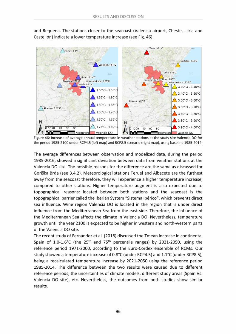
RESULTS AND DISCUSSION
96
and Requena. The stations closer to the seacoast (Valencia airport, Cheste, Llíria and
Castellón) indicate a lower temperature increase (see Fig. 46).
Figure 46: Increase of average annual temperature in weather stations at the study site Valencia DO for the period 1985-2100 under RCP4.5 (left map) and RCP8.5 scenario (right map), using baseline 1985-2014.
The average differences between observation and modelized data, during the period
1985-2016, showed a significant deviation between data from weather stations at the
Valencia DO site. The possible reasons for the difference are the same as discussed for
Goriška Brda (see 3.4.2). Meteorological stations Teruel and Albacete are the furthest
away from the seacoast therefore, they will experience a higher temperature increase,
compared to other stations. Higher temperature augment is also expected due to
topographical reasons: located between both stations and the seacoast is the
topographical barrier called the Iberian System “Sistema Ibérico”, which prevents direct
sea influence. Wine region Valencia DO is located in the region that is under direct
influence from the Mediterranean Sea from the east side. Therefore, the influence of
the Mediterranean Sea affects the climate in Valencia DO. Nevertheless, temperature
growth until the year 2100 is expected to be higher in western and north-western parts
of the Valencia DO site.
The recent study of Fernández et al. (2018) discussed the Tmean increase in continental
Spain of 1.0-1.6°C (the 25th and 75th percentile ranges) by 2021-2050, using the
reference period 1971-2000, according to the Euro-Cordex ensemble of RCMs. Our
study showed a temperature increase of 0.8°C (under RCP4.5) and 1.1°C (under RCP8.5),
being a recalculated temperature increase by 2021-2050 using the reference period
1985-2014. The difference between the two results were caused due to different
reference periods, the uncertainties of climate models, different study areas (Spain Vs.
Valencia DO site), etc. Nevertheless, the outcomes from both studies show similar
results.

RESULTS AND DISCUSSION
97
Comparison of spatial-temporal progress of temperature between Goriska Brda
and Valencia DO
The average difference between observed temperature data (for the period 1985-2016),
and modelled temperature data (until the year 2100) were calculated for each study
site, using the results from two weather stations: Valencia airport (Valencia DO) and Bilje
(Goriška Brda) (see sections 3.4.2 and 3.4.3). The weather stations were chosen due to
their closeness to the study sites. In the Goriška Brda study site, the temperature
increase shows higher values, compared to the Valencia DO study site. This higher
increase at the Goriška Brda site applies with both RCP4.5 and RCP8.5 scenarios. Average
differences between observed and modelized temperatures (1985-2016) are 0.65°C
(under RCP4.5 and RCP8.5) in Goriška Brda and 0.52°C (RCP4.5 and RCP8.5) in Valencia
DO. Hence, there is a relatively strong correlation between the Euro-Cordex climate
models and observations.
Figure 47: Comparing average difference between observation and modelized data for the period 1985-2016 and increase of temperature under projected period 2071-2100, compared to baseline 1985-2014 under RCP4.5 and RCP8.5 scenarios, between Goriška Brda and Valencia DO study sites.
The future temperature model reveals higher values at the Goriška Brda site. The
correlation between observed and modelized temperature during the period 1985-2016
is stronger in Valencia DO site, which generally demonstrates a more accurate climatic
model. Average modelized temperatures in Goriška Brda (1985-2016) tend to indicate
lower values, compared to observation data. The opposite occurs at the Valencia DO
site, where modelized temperatures tend to show higher values, compared to
observation data. The progress of average modelized temperatures starts to diverge
around 2050 and reaches a maximum divergence in 2100 at both study sites. After 2050
the upward trend is greater under RCP8.5 compared to RCP4.5 (see Fig. 48).
0.65 0.65
2.16
3.95
0.52 0.52
1.27
3.02
0.00
0.50
1.00
1.50
2.00
2.50
3.00
3.50
4.00
4.50
Average difference(RCP4.5)
Average difference(RCP8.5)
Increase 1985-2100(RCP4.5)
Increase 1985-2100(RCP8.5)
An
nu
al m
ean
tem
per
atu
re (
°C)
Goriška Brda Valencia DO

RESULTS AND DISCUSSION
98
Figure 48: Progress of observed average annual and modelized temperatures for the period 1985-2100 under RCP4.5 and RCP8.5 scenarios in Goriška Brda and Valencia DO. Valencia DO refers to the weather station Valencia airport in Valencia DO site and Brda refers to the weather station Bilje in Goriška Brda site. Tmean_VLC_observations and Tmean_Brda_observations stand for average annual observations for temperatures, T_mean_ValenciaDO_RCP4.5 and T_mean_Brda_RCP4.5 stand for average annual modelized temperatures under RCP4.5 scenario and T_mean_ValenciaDO_RCP8.5 and T_mean_Brda_RCP8.5 stand for average annual modelized temperatures under RCP8.5 scenario.
The temperature anomaly depicts a similar, increasing trend at both study sites for the
period 1985-2100. The two temperature anomalies under RCP8.5 start to diverge from
temperature anomalies under RCP4.5 around the year 2050. Afterwards, they escalate
until 2100, when they reach the highest difference. The correlation between
temperature anomalies at both study sites under RCP4.5 is stronger, compared to
temperature anomaly under RCP8.5 (see Fig. 49).
10
12
14
16
18
20
22
19
85
19
90
19
95
20
00
20
05
20
10
20
15
20
20
20
25
20
30
20
35
20
40
20
45
20
50
20
55
20
60
20
65
20
70
20
75
20
80
20
85
20
90
20
95
21
00
An
nu
al m
ean
tem
per
atu
re (
°C)
Tmean_ValenciaDO_observations Tmean_ValenciaDO_RCP4.5Tmean_ValenciaDO_RCP8.5 Tmean_Brda_observationsTmean_Brda_RCP4.5 Tmean_Brda_RCP8.5

RESULTS AND DISCUSSION
99
Figure 49: Average annual temperature anomaly for the period 1985-2100 at the Goriška Brda and Valencia DO study sites according to RCP4.5 and RCP8.5 scenarios. Valencia DO refers to the weather station Valencia airport in Valencia DO site and Brda refers to the weather station Bilje in Goriška Brda site. Anomaly_Brda_RCP4.5 and Anomaly_ValenciaDO_RCP4.5 stand for temperature anomaly from baseline period 1985-2014 under RCP4.5 scenario, Anomaly_Brda_RCP8.5 and Anomaly_ValenciaDO_RCP8.5 stand for temperature anomaly from baseline period 1985-2014 under RCP8.5 scenario. Solid lines present the 10 years average value.
The temperature increase for the projected period 2071-2100, compared to baseline
period 1985-2014, presents a significant impact on viticulture at both study sites in the
future: between 1.27°C (RCP4.5) and 3.02°C (RCP8.5) in Valencia DO and between 2.16°C
(RCP4.5) and 3.95°C (RCO8.5) in Goriška Brda. The temperature growth indicates similar
values at both study sites. Nevertheless, Valencia DO site is expected to be more
affected by the temperature increase in the future, due to a considerably higher present
temperature: the average daily Tmean for the period 1985-2016 was 5.14°C higher at
the Valencia DO site, compared to Goriška Brda. Hence, the Valencia DO site will
experience a higher environmental impact. From an economic standpoint, the viability
of viticulture at this site will be at stake.
Temporal precipitation analysis in Goriška Brda and Valencia DO
Average difference between the observed and modelized precipitation is significantly
higher at the study site Goriška Brda, compared to Valencia DO, for the period 1985-
2016. Precipitation levels almost double at the Goriška Brda site under both forcing
scenarios. The future precipitation trend for the projected period 2071-2100, compared
to the baseline period 1967-1996, reveals a lower, negative trend in Valencia DO.
Goriška Brda will enjoy a positive increase in rainfall (4.41 mm, under RCP4.5), which is
the only positive growth until the year 2100. The calculated projections show an almost
double decrease of rainfall in Valencia DO under RCP8.5 scenario, compared to RCP4.5.
Nevertheless, the difference between forcing scenarios at the Goriška Brda site is higher.
Under RCP8.5 scenario, the precipitation will decrease by almost three times of that
shown under the RCP4.5 scenario (see Fig. 50).
-1
0
1
2
3
4
5
19
85
19
90
19
95
20
00
20
05
20
10
20
15
20
20
20
25
20
30
20
35
20
40
20
45
20
50
20
55
20
60
20
65
20
70
20
75
20
80
20
85
20
90
20
95
21
00
An
nu
al a
vera
ge t
emp
erat
ure
(°C
)Anomaly_Brda_RCP4.5
Anomaly_Brda_RCP8.5
Anomaly_ValenciaDO_RCP4.5
Anomaly_ValenciaDO_RCP8.5

RESULTS AND DISCUSSION
100
Figure 50: Difference between observed and modelized precipitation for the period 1985-2016 at both study sites (four bar charts on the left). Increase of precipitation under projected period 2071-2100, compared to observed baseline (1967- 1996) under RCP4.5 and RCP8.5 scenarios (four bar charts on the right).
Observations of precipitation fluctuation show a considerably higher amplitude,
compared to models (RCP4.5 and RCP8.5) during the reference period 1985-2016. The
intensity of precipitation amplitude is higher at the Goriška Brda site and especially
peaks in the years 2010, 2011 and 2015. Hence, the average difference between
observed and modelized precipitation is greater, compared to Valencia DO. Most of the
observed and modelized peaks are synchronized at both study sites, which suggests a
relatively high correlation with the climate model. The progress of modelized
precipitation, under RCP4.5 and RCP8.5 scenarios, share a similar moderate tendency at
in both study sites. However, both precipitation models reveal higher amplitude at the
Goriška Brda site (see Fig. 51).
253.99 255.89
4.41
-9.89
134.94148.77
-56.11-83.45
-150.00
-100.00
-50.00
0.00
50.00
100.00
150.00
200.00
250.00
300.00
Average difference(RCP4.5)
Average difference(RCP8.5)
Increase 1967-2100(RCP4.5)
Increase 1967-2100(RCP8.5)
Pre
cip
itat
ion
(m
m)
Goriška Brda Valencia DO

RESULTS AND DISCUSSION
101
Figure 51: Progress of observed average annual and modelized precipitation under RCP4.5 and RCP8.5 scenarios for the period 1985-2100 in Goriška Brda and Valencia. P_VLC_observations stands for average annual observations of precipitation at weather station Valencia airport (Valencia DO), P_Brda_observations stands for average annual observations of precipitation at weather station Bilje (Goriška Brda), P_VLC_RCP4.5 stands for average annual modelized precipitation at weather station Valencia airport (Valencia DO) under RCP4.5 scenario, P_VLC_RCP8.5 stands for average annual modelized precipitation at weather station Valencia airport (Valencia DO) under RCP8.5 scenario, P_Brda_RCP4.5 stands for average annual modelized precipitation at weather station Bilje (Goriška Brda) under RCP4.5 scenario and P_Brda_RCP8.5 stands for average annual modelized precipitation at weather station Bilje (Goriška Brda) under RCP8.5 scenario.
The fluctuation in precipitation between the two study areas shows a significant
difference. Goriška Brda enjoys largely regular precipitation throughout the whole year
totalling about 1500 mm per annum (Ažman et al., 2008; Gorjak, 2017), in contrast to
Valencia DO where rainfall throughout the year is irregular. Most of the precipitation
occurs at the end of summer, due to the meteorological phenomenon called “Gota fria”
(Confederación Hidrográfica del Júcar, 2019). The annual present precipitation is about
424 mm (IVIA, 2017), which is about 1076 mm less than in Goriška Brda. Differences
between observed and modelized precipitation during the reference period 1985-2016,
were elevated at both sites, especially at the Goriška Brda site. Nevertheless, the the
progress of the observed and modelized precipitation levels show a synchronized trend,
which confirms the reliability of the precipitation model. The precipitation trend under
both forcing sceneries (RCP4.5 and RCP8.5) shows no significant increase, or decrease,
until the year 2100 at both study sites. Nevertheless, the extreme precipitation, along
with other extreme meteorological events due to the climate change (IPCC, 2018), are
expected at both wine making sites. At the present time, there is almost no irrigation in
Goriška Brda, however irrigation is a common practice in Valencia DO. A stronger
environmental impact will therefore be experienced in Valencia DO due to less
precipitation in the future, compared to Goriška Brda, which already enjoys almost three
times more rainfall (Gorjak, 2017, IVIA, 2017). The combination of temperature increase
and precipitation decrease will affect the economic prospects for viticulture in Valencia
DO and, without successful adaptation, its future will become uncertain. According to
the ENSEMBLES project (Van Der Linden & Mitchell, 2009), the average change in
0
500
1000
1500
2000
2500
19
67
19
72
19
77
19
82
19
87
19
92
19
97
20
02
20
07
20
12
20
17
20
22
20
27
20
32
20
37
20
42
20
47
20
52
20
57
20
62
20
67
20
72
20
77
20
82
20
87
20
92
20
97
Pre
cip
itat
ion
(m
m)
P_VLC_observations P_VLC_RCP4.5P_VLC_RCP8.5 P_Brda_observationsP_Brda_RCP4.5 P_Brda_RCP8.5

RESULTS AND DISCUSSION
102
precipitation under the projected period 2021-2050, will increase by 0-1%, compared to
the baseline period 1961-1990 in Goriška Brda. The results of this thesis show a 4%
decrease, the average under RCP4.5 and RCP8.5 scenarios. Considering the reference
period was not the same, the difference between the predictions was less than 5%,
which make our results comparable to the results from the ENSMBLES project. The study
of Fernández et al. (2018) showed an average precipitation decrease in continental Spain
of 0.25-10.5% (the 25th and 75th percentile ranges) by 2021-2050 using the reference
period 1971-2000, according to the Euro-Cordex ensemble of RCMs (Jacob et al., 2014).
Our study showed a decrease in rainfall at the Valencia DO site of 6.0% (RCP8.5) and
6.8% (RCP4.5) by 2021-2050, using the same reference period. The results of this thesis
fit roughly in the middle of the range showed in the Fernández (2018) study. The
difference between the two sets of results was most probably due to different study
area locations (Spain vs. Valencia DO site), the uncertainties of climate models and
different methodologies. Nevertheless, the results from both studies are similar.
3.5 Analysis 5: Assessment of viticultural potential and delineation in Goriška
Brda
Analysis of the viticultural potential of Goriška Brda was conducted by using the
methodology described in the Methodology section (see 2.11). The results are divided
into three sections. The first section describes the results of the GIS analysis of the
spatial distribution of topographical, climatic and pedological factors. The second part
shows the results of suitability distribution in numerical tables. Finally, the third section,
presents the spatial distribution of topographical, climatic and pedological suitability for
different quality wines, according to the evaluation system described in Table 14. Results
are presented on several maps of viticultural potential for each suitability category:
topographical, pedological and climate. Each category map spatially defines areas for
growing grape with a different purpose: from zones not suitable for grape growing, to
zones suitable for quality red wine production. Emphasis is made on the final suitability
map, which reflects a combination of the topographical, pedological and climate
suitability maps. Topography, soil and climate have a strong influence on vine
performance (Fraga et al., 2014), hence it is significant to study all three concepts in
order to enhance the wine quality.
Spatial distribution of topographical, pedological and climatic factors
To increase the understanding of data, and the results of the research, the study area
was roughly divided according to slope and topography characteristics into two zones,
designated as Higher (HZ) and Lower zone (LZ) (see Fig. 52a and Fig. 52b). The HZ is
characterized by slopes predominantly higher than 6%, and where a majority of terrain
is higher than 200 m asl. The LZ is characterized by slopes that are mainly less than 6%
and where a majority of terrain is lower than 200 m asl. Most of the vineyards are
located in the LZ, due to preferable warmer conditions for grape production. There are
four major ridges which run north-east (NE) towards the south-west (SW) and are

RESULTS AND DISCUSSION
103
residues from alpine orogenesis (Placer, 1981; Fikfak et al., 2017) (see Fig. 52c).
Topographical factors show high variability of terrain in the whole study area. The
terrain reveals predominantly SW and southern aspects, on 45.14% of the study area.
Most of the areas with southern aspects are located in the eastern part. Areas with a
mostly northern aspect, are distributed throughout the entire study area, however, the
central and western part contains a higher concentration. Most of the plain areas are
located in the southern part. Areas with a western and eastern aspect are
homogeneously distributed. The variability in altitude of the study site is rather
moderate, since a majority of the terrain is characterised by a 6% slope (see Fig. 52d).
Figure 52: Maps of spatial distribution of topographical factors in Goriška Brda (Brda): (a) map of DEM (expressed in m asl); (b) map showing partition of LZ and HZ with major villages; (c) map of topographical aspect (expressed as H (horizontal), N (northern), NE (north-eastern), E (eastern), SE (south-eastern), S (southern), SW (south-western), S (southern), SE (south-eastern), W (western) and NW (north-western); and (d) aspect and map of slope (expressed in slope percentage).
The humus content varies between a minimum of 0.54% to a maximum of 6.64%. Higher
levels of humus are located in the extreme eastern and northern part (see Fig. 53a). Soil
with the highest clay content is found in the eastern and NE part (see Fig. 53b). Clay
concentration levels in soils gradually decrease from maxims of 32.63% in the NE to
minims of 26.71% towards the SW part of Brda. Soils with the highest gravel content are
found in the eastern part and decrease slowly from 34.84% to 12.17% towards the south
(see Fig. 53c).

RESULTS AND DISCUSSION
104
Figure 53: Maps of pedological factors of Brda: Map of contents of humus (a), clay (b) and gravel (c). All values are expressed in percentage of pedological factor’s content in the soil.
With regard to climatic factors, spatial distribution of AAT reveals higher values (12.4°C)
in the LZ, compared to the HZ where the minimum is 8.1°C (see Fig. 54a). The TWM show
similar spatial distribution of maximum (22.3°C) in LZ and minimum temperatures in HZ
(see Fig. 54b). The SET, IAOe and IHa, being based on temperature, show relatively
similar spatial distributions, where maximum values are in the LZ, and gradually diminish
towards the NE part of the HZ (see Fig. 54c, Fig. 5d and Fig. 5e). Due to the altitudinal
gradient of 0.65°C, the spatial distribution of AAT, TWM and SET values depict a gradual
diminishment from the LZ towards higher latitudes in the HZ. Bioclimatic indices SET,
IAOe and IHa show nearly double values in the LZ, compared to the HZ: with values of
1521, the SET shows the LZ to have the highest viticultural potential in contrast to only
a few limited areas at higher altitude (approx. 200 m asl) in the north and south-east
(SE) areas of Brda. Areas with higher hours of ASD (see Fig. 54f) are located in elevated
areas (1451h) in the north, especially on southern slopes; lower values reach (813h) in
northern slopes mostly in the HZ. The potential sunshine duration (PSD) depicts a similar
spatial distribution with nearly double values (See Fig. 54g). Actual GR shows higher
values (101 kcal/cm2) on southern slopes and lower values on northern slopes (27
kcal/cm2) (See Fig. 54h). Spatial distribution of global potential radiation depicts similar
a spatial distribution (See Fig. 54i).

RESULTS AND DISCUSSION
105
Figure 54: Maps of climatic factors and indices of Brda. All values represent average values during growing season for the period 1980-2014. Map (a) represents AAT, and map (b) TWM. Maps (c), (d) and (e) depict bioclimatic indices SET, IAOe and IHa, respectively. ASD and PSD are represented in maps (f) and (g), respectively. Actual and global potential radiation are shown in maps (h) and (I), respectively. Map (j) indicates PP, and map (k) LGS.

RESULTS AND DISCUSSION
106
Figure 54 (continuation): Maps of climatic factors and indices of Brda. All values represent average values during growing season for the period 1980-2014. Potential radiation is shown in map (i), map (j) indicates PP and map (k) LGS.
PP during the growing season shows more abundant rainfall in the HZ (1343 mm),
compared to the LZ (707 mm) (See Fig. 54j). This is equally beneficial for yield size and
grape quality, taking into account the high values of heliothermic factors in the area,
which can lead to severe evapotranspiration and water deficit, especially in lower areas.
LGS is significantly longer in the LZ, up to 212 days per year, compared to the HZ, where
it reaches the minimum of 157 days, practically insufficient for the maturation of grapes.
The higher value of 212 days, reveal conditions for maturing grapes, including late
varieties, lasting over 190 days (See Fig. 54k).
Each environmental factor represents an essential part in spatial analysis of viticultural
potential. Furthermore, spatial distribution of environmental factors, and their
suitability, represent an essential tool to elaborate the viticultural potential of Brda.
According to the topographical factors, the most appropriate areas suitable for quality
red wine production (class I) are located on the terrains with southern, SW and SE
aspects, which are located mostly in the HZ. According to the slope characterization, the
most suitable areas for quality grape production (class I) are located close to the valley
bottoms. Nevertheless, the predominant class II covers 81.19% of the entire study site.

RESULTS AND DISCUSSION
107
The viticultural potential for the production of white table and sparkling wines and wines
for distillates (class III) are located in the valley bottoms. The most favourable areas for
red quality wine (class I) according to the humus content, are mostly in the LZ and,
according to the gravel content, in the whole study site, accept in the NE part of the HZ.
The clay content in soils shows the entire Brda region is suitable for the production of
quality white wines. According to the pedological factors, there were no areas
unsuitable for grape and wine production.
The variation of temperature at altitude has a significant impact on grape production
(Herrera Nuñez et al., 2011). Spatial variability of temperature is manifested by a
difference in altitude. According to AAT, the highest viticultural potential is distributed
across the entire study site, with the exception of the NE part of the HZ. Environmental
factor TWM shows the areas suitable for the cultivation of quality red wine are mostly
in the LZ. Areas with a higher altitude (NE part) reveal an inferior viticultural potential,
in comparison to areas with a lower altitude. Moreover, high topographical variability in
altitude shows an AAT 4.3°C higher in eastern part of study site, compared to southern
part. A similar difference (4.5°C) is shown with the TWM. Higher values of actual and
PSD are found on northern exposures with lower values on southern exposures.
According to the suitability of sunshine duration, there are two areas in Brda. Areas on
the northern slopes are suitable for the production of white table wines (class III),
however southern slopes are not suitable for viticulture.
Distribution of actual and potential global radiation is on the opposite aspect to actual
and PSD. It shows higher values on southern slopes and lower ones on northern slopes.
Values of global potential radiation are approx. 15% higher, compared to actual GR
across the whole study site. The majority (56.92%) of areas suitable for quality red wine
(class I) are distributed on southern slopes. Most of the northern slopes are
characterized as areas not suitable for vine growing. Areas suitable for grape production
for lower wine quality (white table wine and quality white wine) are distributed mostly
on northern slopes, nevertheless, this viticultural potential represents only 21.36 % of
the study area. Precipitation during the growing season has varies significantly, by 636
mm, showing a high precipitation variability in a relatively small area. Areas with inferior
precipitation are located in the plains, especially in the LZ. The amount of precipitation
increases gradually towards higher areas: the maximum is located in the NE and eastern
parts of the HZ.
Distribution of LGS shows higher values in the LZ and in the lower parts of the valleys.
Areas in the extreme NE and extreme eastern part of the HZ have a shorter number of
days. A large part of the area (80.17%) has LGS suitability for quality red wine class I.
Areas with lower viticultural potential are located in the extreme eastern part of the HZ.
Similar results of the spatial analysis of the environmental characteristics of Brda were
reported by Fikfak et al. (2017).
Suitability of topographical, pedological and climatic factors
The structure of suitability for grapevine growing for each environmental parameter is
shown in Table 30 and Table 31. The structure is determined according to the limits and

RESULTS AND DISCUSSION
108
classes mentioned in Table 15. The spatial distribution of slope suitability shows that
most of the Brda district is characterised by class II (slopes greater than 15%, difficult to
work), and only 9% for both of the I and III classes. This is specific to the Piedmont region,
with ragged terrains. Regarding the terrain aspect, nearly half of the surface is defined
as class I (SW, south, SE), that assures high values of heliothermal parameters and is very
suitable for grape quality; class II at 25% (eastern, western and horizontal aspects) is less
suitable, and class III at 29% (NW, north and NE) the least suitable. In the context of
climate change, when the values of heliothermal factors become excessive on southern
aspects, it is possible, that northern aspects become more suitable, so that the high
percentage of the present northern aspects can be appreciated as a future reserve of
suitability for Brda region.
Table 30: Topographical and pedological factors and their related environmental parameters with their
suitability intervals.
Environmental category
Environmental parameters
Suitability Surface and percentage of Goriška Brda
intervals classes ha %
Top
ogr
aph
ical
fa
cto
rs
Slope (%) 8-15 I 673.06 9.36 >15 II 5839.39 81.19 <8 III 679.83 9.45
Aspect SW, S, SE I 3246.88 45.14 E, W, horizontal
II 1823.65 25.36
NW, N, NE III 2121.75 29.50
Pe
do
logi
cal f
acto
rs
Clay content (%) 15-25 I 0 0 25-40 II 7192.28 100.00 <15 III 0 0 >40 IV 0 0
Humus content (%)
1.5-2.0 I 3270.01 45.47 2.1-3.0 II 1739.45 24.19 3.1-4.5 III 2182.79 30.35
Gravel content (%) 10-30 I 6952.06 96.66 30-40 II 240.22 3.34 <10 III 0 0 >40 IV 0 0
The clay content for the entire Brda region is characterised by class II, suitability for
white quality wines, while other classes are not represented. The humus content is
characterised by class I - suitability for red quality wines for about half of the surface,
while class II (quality white wines) and class III (table white wines) are represented with
similar shares of about 24.19% and 30.35% respectively. This humus content has thus a
very balanced spatial distribution, which favors the cultivation of different wine varieties
and the production of different wine types, even in the case of the same variety. In the
context of climate change and temperature increases, a larger humus content may
become suitable for grape quality, supporting canopy development and protection of
the grapes chemical composition by shading (Palliotti et al., 2011). The large gravel

RESULTS AND DISCUSSION
109
content of Brda soils characterises the entire area as class I, that means that it has a
large potential to produce high quality wines, from both red and white varieties. Table 31: Climatic factors with their environmental parameters with their suitability intervals.
Environmental category
Environmental parameters
Suitability Surface and percentage of Brda
intervals classes ha %
C
limat
ic f
acto
rs
AAT (°C) 10.0-11.2 I 6769.50 94.12 9.4-10.0 II 262.74 3.65 8.5-9.3 III 138.91 1.93 <8.5 IV 21.14 0.29
TWM (°C) 21.0-22.0 I 4792.50 66.63 19.8-21.0 II 1993.02 27.71 18.1-19.0 III 400.63 5.57 <18.0 IV 6.12 0.09
SET 1401-1675 I 2797.27 38.89 1201-1400 II 3099.40 43.09 1045-1200 III 1008.89 14.03 <1045 IV 286.72 3.99
IAOe >4600 I 0 0 4301-4600 II 0 0 3793-4300 III 3226.27 44.86 <3793 IV 3966.01 55.14
IHa 2.21-2.66 I 0 0 1.71-2.20 II 3151.58 43.82 1.36-1.70 III 3517.85 48.91 <1.36 IV 522.86 7.27
LGS (days) >190 I 5766.17 80.17 176-190 II 1201.77 16.71 160-175 III 213.10 2.96 <160 IV 11.23 0.16
GR (kcal/cm2) 87.0-92.0 I 4093.98 56.92 84.0-86.9 II 721.51 10.03 80.0-83.9 III 814.67 11.33 <80.0 IV 1562.13 21.72
ASD (hours) 1551-1610 I 0 0 1451-1550 II 6.93 0.10 1280-1450 III 1664.54 23.14 <1280 IV 5520.82 76.76
PP (mm) 251-390 I 7192.28 100.00 <250 II 0 0 >390 III 0 0
AAT, average annual temperature; TWM, average temperature of the warmest month; SET, sum of effective temperatures; IAOe, oenoclimatic aptitude index; IHa, actual heliothermal index; LGS, length of the growing season; GR, global radiation; ASD, actual sunshine duration; PP, precipitation in the growing season.
The precipitation volume classifies the entire study site as class III, suitability for white
table wines. However, this high level is suitable in the context of climate change, when
temperature increases determine a more accentuated evapotranspiration, exposing
vines to water deficit. So, as in the case of high humus content, the water abundance

RESULTS AND DISCUSSION
110
can represent a control factor for microclimate suitability and a reserve for future
climate evolutions. The AAT classifies 66.63% of the area as class I, values higher than
21 °C, showing enough thermal resources for grape ripening. At the same time, in the
context of climate change, this parameter can increase and become detrimental to
grape quality, by hastening ripening and disturbing the grapes balanced chemical
composition. The SET, that assesses effective temperatures during the growing season,
characterises 38.89% of the surface as class I, 42.09% as class II, and 14% of the study
area as class III. Regarding the GR, more than a half of the surface shows characteristics
of class I, while other classes are each characterised by between 10-20% of the surface.
The ASD seems to be the most deficient factor in the Brda area, with about 76% of the
surface characterised by class IV, practically unsuitable for efficient grape growing.
However, due to the large values of all the other heliothermal parameters, characteristic
to regions influenced by Mediterranean climate, this deficit is compensated, and thus
makes the area suitable for grape growing. The lower values of the ASD also significantly
affect the bioclimatic indices suitability, that is largely variable in the Brda region, as
follows: The IHa indicates that 48.91% of the surface is entitled to class III, 43.82% to
class II, while only 7.27% to class IV and 0% to class I. Furthermore, the IAOe, classify
55.14% of the Brda area as class IV and 44.86% as class III. The low suitability of
bioclimatic indices is caused by the ASD deficit, meaning grape growing should be
practiced on sunny surfaces in the Brda region.
Spatial distribution of suitability
Suitability is defined by the average of the ranking points for the factor’s suitability in
each environmental category - topographical, climate and pedological. Topographical
suitability, given by the slope and aspect suitabilities, reveals that approx. 43.31% of the
Brda surface is entitled to class I (see Table 32) – revealing environmental conditions for
the production of red and white quality wines. Less than 30% of the area is characterised
as class II and III – suitability for white quality wines and white table wines, while class
IV is not observed.
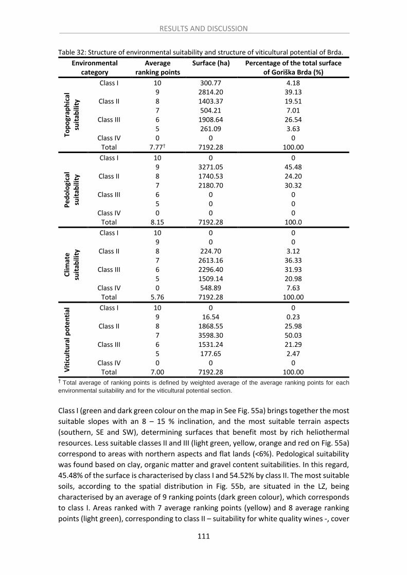
RESULTS AND DISCUSSION
111
Table 32: Structure of environmental suitability and structure of viticultural potential of Brda.
Environmental category
Average ranking points
Surface (ha) Percentage of the total surface of Goriška Brda (%)
Top
ogr
aph
ical
suit
abili
ty
Class I 10 300.77 4.18 9 2814.20 39.13
Class II 8 1403.37 19.51 7 504.21 7.01
Class III 6 1908.64 26.54 5 261.09 3.63
Class IV 0 0 0 Total 7.77† 7192.28 100.00
Pe
do
logi
cal
suit
abili
ty
Class I 10 0 0 9 3271.05 45.48
Class II 8 1740.53 24.20 7 2180.70 30.32
Class III 6 0 0 5 0 0
Class IV 0 0 0 Total 8.15 7192.28 100.0
Clim
ate
suit
abili
ty
Class I 10 0 0 9 0 0
Class II 8 224.70 3.12 7 2613.16 36.33
Class III 6 2296.40 31.93 5 1509.14 20.98
Class IV 0 548.89 7.63 Total 5.76 7192.28 100.00
Vit
icu
ltu
ral p
ote
nti
al Class I 10 0 0
9 16.54 0.23 Class II 8 1868.55 25.98
7 3598.30 50.03 Class III 6 1531.24 21.29
5 177.65 2.47 Class IV 0 0 0
Total 7.00 7192.28 100.00 † Total average of ranking points is defined by weighted average of the average ranking points for each
environmental suitability and for the viticultural potential section.
Class I (green and dark green colour on the map in See Fig. 55a) brings together the most
suitable slopes with an 8 – 15 % inclination, and the most suitable terrain aspects
(southern, SE and SW), determining surfaces that benefit most by rich heliothermal
resources. Less suitable classes II and III (light green, yellow, orange and red on Fig. 55a)
correspond to areas with northern aspects and flat lands (<6%). Pedological suitability
was found based on clay, organic matter and gravel content suitabilities. In this regard,
45.48% of the surface is characterised by class I and 54.52% by class II. The most suitable
soils, according to the spatial distribution in Fig. 55b, are situated in the LZ, being
characterised by an average of 9 ranking points (dark green colour), which corresponds
to class I. Areas ranked with 7 average ranking points (yellow) and 8 average ranking
points (light green), corresponding to class II – suitability for white quality wines -, cover

RESULTS AND DISCUSSION
112
the northern and NE part of the Brda site, while the eastern part is characterised by 7
ranking points – suitability for white quality wines.
Figure 55: Map of topographical (a), pedological (b), climate (c) and final (d) suitability. Ranking points definition: 4 stands for areas unsuitable for grape production, 5 stands for areas suitable for white table wines, sparkling wines and wines for distillates, 6 stands for areas suitable for white table wines, sparkling wines, wines for distillates and for white quality wines, 7 stands for areas suitable for white quality wines, 8 stands for areas suitable for quality white wines and secondary for red table wines, 9 stands for areas suitable for red quality wines and secondary for white quality wines and 10 stands for areas suitable for quality red wines.
Regarding climate suitability, 52.91 % of the Brda area is characterised by class III, while
39.45% of the area by class III (See Fig. 55c). 7.63% of the Brda area has a climate
unsuitable for grape growing, characterised by class IV. Climate suitability varies from
unsuitable, 4 points (black on the map) to 8 average points (green), while 36.33% of the
area is characterized by 7 ranking points (yellow). The very suitable area is situated in
the LZ of Brda (See Fig. 55c). Areas, corresponding to class III, are located in the HZ of
the studied area, especially with northern and NE aspects.
The map of viticultural potential of the Brda area, resulting from the suitability of soil,
relief and climate is shown in Fig. 55d. The data shows that the whole Brda wine region
is suitable for grapevine growing. The largest part of the Brda area (76.01%) is
characterised by class II and 23.76% by class III. Only 0.23% of the Brda surface (shown
green) is characterised by class I (with 9 ranking points). Within the Brda area there are
no surfaces characterised by an average of 10 ranking points. The areas corresponding

RESULTS AND DISCUSSION
113
to the class I are represented by 16.73 ha, situated in the LZ. Class II – 8 ranking points,
suitability for white quality wines and red table wines - (light green on map)
characterises 1861 ha of the Brda area, mostly in the LZ. Areas characterised by 7 ranking
points, suitability for quality white wines (yellow on map), are scattered on 3584 ha
across the entire Brda area, especially on northern aspects. The extreme northern area,
with about 1701 ha (orange and red), is characterised by class III – suitability for white
table wines, sparkling wines and quality white wines in the very suitable years.
The highest suitability is revealed under the topographical category, where 4.18% of the
entire study area, dispersed on southern terrain aspects, is characterised by an average
of 10 ranking points. The topographical suitability characterizes 43.31% of Brda as a wine
growing zone suitable for grape production for high quality red and white wine, located
mostly in the HZ, with a southern aspect. Zones with inferior topographical suitability
are located in areas with a northern aspect. There are no zones unsuitable for vine
growing. In a similar study in Romania (Irimia et al., 2014), southern aspects also show
higher viticultural potential, compared to northern aspects. Second highest suitability is
in the pedological category, suggesting areas suitable for red and white quality wines
and red table wine production (class I and class II). The surface of the zone suggesting
quality red and white wine production (class I) is located mostly in the LZ and it covers
nearly the half of the entire study site. Areas suggested for production of white quality
and table wines including red table wines (Class II), cover 54.52% of Brda and are located
mostly in the HZ.
Climate suitability analysis suggests the largest amplitude of ranking points: from 1 to 9.
The zones with the highest suitability, suitable for red and white quality wine production
are characterized by class II (39.45% of the surface of the study site) and are located
mostly in the LZ. The lowest climate suitability corresponds to areas in the HZ in the
extreme northern part. The zones suitable for quality red and white wine production are
situated in the LZ, suggested by all three spatial analyses, roughly estimated. The
topographical suitability analysis also suggests areas with a southern aspect in the HZ
are areas with high viticultural potential (class I), whereas pedological and climate
suitability analyses clearly do not recommend these areas for grape growing for quality
wine production. According to the final suitability analysis, zones suitable for quality red
and white wine production correspond to the areas with a mostly southern aspect,
located in the LZ. Zones suitable only for white quality wine production are found in the
LZ, in areas with northern aspect, and in the HZ, in areas with a southern aspect.
Production of white and red table wine correspond to areas with a northern aspect in
the HZ. The grape varieties most represented in Brda are white varieties Rebula, Ribolla
Gialla and Chardonnay, making up 65% of all the grape varieties for production year
2011 (Zamar, 2013), which confirms the results of this study.
In the study by Rusjan and Korošec-Koruza (2003), a delineation analysis was conducted,
assessing Brda using Winkler, Branas, Huglin, Kerner and Seljaninov indices, which
characterized four different viticultural zones and suggested Brda as a terroir. The
homogeneous zones were defined by average sugar index of grapes. Using a higher
number of environmental factors, and a different methodology using GIS tools, allowed
us to conduct more detailed spatial analysis. The results discussed in this paper present

RESULTS AND DISCUSSION
114
a higher number of zones with more detailed classification of viticultural potential of
newly defined homogeneous zones.
3.6 Analysis 6: Assessment of WR in Valencia DO (1985-2100)
In this section are presented the results of elaborating the model of WR for Tempranillo,
Bobal and Moscatel varieties in the vinegrowing region Valencia DO. In the first part, the
results of modelling ETo by using FAO BC formula and temporal analysis of DI are
discussed. In the second part, are discussed the results of WR modelling for the
Tempranillo, Bobal and Moscatel grape varieties, for the period 1985-2100.
Reference evapotranspiration model
Using the observation dataset from Llíria weather station (see Table 5 and Fig. 16), was
calculated the ETo model for the period 2000-2016 using BC method (EToBC). The EToBC,
derived from PM method (EToPM), the assumed standard method, was used to assess
the results obtained for EToBC. The comparison analysis between BC and PM
methodologies was conducted for the analysis period 2000-2016. EToBC fluctuation
shows, on average, 173 mm higher values, compared to EToPM, however, an increasing
and decreasing tendency for both ETo, occurs simultaneously. The goal was the
reduction of the difference between EToBC and EToPM. The corrections were achieved by
correction bias method using the correction factor δ (Hay, Wilby, & Leavesley, 2000).
Newly corrected EToBC_C indicates an average difference with EToPM of less than 1 mm.
The values a and b (see 2.12.1.1), were not changed, because they derivate from climate
parameters. The modelized EToBC, derived from Euro-Cordex datasets under RCP4.5 and
RCP8.5 scenarios, were corrected using the correction factor δ. The tendency of the
corrected EToBC_C under both climate scenarios reveals similar progress during the
period 2000-2016, compared to reference EToPM: rising and dropping occurs
simultaneously (see Fig. 56).

RESULTS AND DISCUSSION
115
Figure 56: Comparison of modelized and observed ETo during the observation period 2000-2016. ETo_BC stands for EToBC (ETo derived from BC formula), ETo_RCP4.5 stands for EToBC model using BC formula under RCP4.5 scenario, ETo_RCP8.5 stands for EToBC model using BC formula under RCP8.5 scenario, ETo_PM stands for EToPM (ETo derived from PM formula) using observation data from IVIA and ETo_BC_corrected stands for EToBC_C , corrected EToBC.
The mean square error (MSE) and mean absolute percentage error (MAPE) demonstrate
stronger correlation between corrected EToBC_C and reference EToPM, compared to
correlation EToBC and EToPM. The MSE between EToBC_C and EToPM indicates value 0.02,
which shows a significantly higher correlation, compared to MSE between EToBC and
EToPM (0.24). Furthermore, the MAPE between EToBC_C and EToPM indicates 3.76%, which
confirms a stronger correlation, compared to MAPE between EToBC and EToPM (15.88%).
In order to qualitatively validate the EToBC_C, it was statistically tested with two other
ETo methods, which are used in the case of missing data and do not require the full
dataset as PM. The comparison period was defined from 2000 to 2016. The compared
methods were: ETP Penman (Penman, 1948) and ETH Hargreaves (Hargreaves, 1982) (see
Fig. 57).
1000
1050
1100
1150
1200
1250
1300
1350
2000 2001 2002 2003 2004 2005 2006 2007 2008 2009 2010 2011 2012 2013 2014 2015 2016
mm
/yea
r
ETo_BC ETo_PM ETo_BC_corrected
ETo_RCP4.5 ETo_RCP8.5

RESULTS AND DISCUSSION
116
Figure 57: Comparison of several ETo using different methods. ETo_Penman stands for EToP (derived from Penman method) using observation data, ETo_PM stands EToPM (derived from Penman-Montheith formula) using observation data, ETo_BC_corrected stands for EToBC_C corrected EToBC with correction factor 𝛿 , ETo_Hargreaves stands for EToH (derived from Hargreaves formula) using observation data and ETo_BC stands for EToBC (derived from BC formula) using observation data retrieved from IVIA (IVIA, 2017).
All compared methods show a positive trend and similar progress during the comparison
period. EToP indicates the highest amplitude and the highest values, since it has
tendency of overestimation of ETo values, as discussed by FAO-56 (Allen et al., 1986).
The lowest values amongst them all, indicates EToPM. Moreover, EToBC_C determines the
strongest correlation with the EToPM, defined by root mean square error (RMSE) of 0.13
and annual average relative error (AARE) of 3.76%. According to the RMSE and AARE,
the weakest correlation, compared to EToPM, shows EToP, followed by EToH and EToBC
(see Table 33).
Table 33: Statistical comparison between EToPM and four other ETo derived from different methods: EToBC (Blaney-Criddle), EToH (Hargreaves), EToP (Penman) and EToBC_C (corrected Blaney-Criddle).
ETo method Statistical error
Annual average relative error
Root mean square error
BC 15.88 0.49 BC corrected 3.76 0.13 Hargreaves 14.82 0.46 Penman 25.02 0.77
The BC formula was used for the future model calculation of ETo models, under RCP4.5
(EToRCP4.5) and RCP8.5 (EToRCP8.5), due to its robust nature and available dataset (see
2.12.2). EToRCP4.5 and EToRCP8.5 scenarios depict a constant positive trend during the
analysis period 1985-2100. They also suggest strong correlation until 2057, roughly
estimated, when the models start to diverge: EToRCP8.5 indicates a higher rise than
800
900
1000
1100
1200
1300
1400
1500
1600
1700
2000 2001 2002 2003 2004 2005 2006 2007 2008 2009 2010 2011 2012 2013 2014 2015 2016
mm
/yea
rETo_Penman ETo_Hargreaves
ETo_PM ETo_BC
ETo_BC_corrected

RESULTS AND DISCUSSION
117
EToRCP8.5. The growth of the ETo model, according to the trendline, increases by up to
110 mm under RCP4.5 and 234 mm under RCP8.5 scenario, during the study period
1985-2100 (see Fig. 58).
Figure 58: ETo models progress, where ETo_model_RCP4.5 and ETo_model_RCP8.5 stands for EToRCP4.5 and EToRCP8.5, respectively. Both models were derived from BC formula using Euro-Cordex dataset. ETo_BC_corrected stands for EToBC_C (corrected EToBC calculated by BC formula) using observation dataset.
There is a notable difference between EToBC_C and modelized ETo (EToRCP4.5 and
EToRCP8.5), which is caused mainly by the uncertainty of the climate models and its spatial
resolution (see 1.4.2). The correlation between modelized ETo and EToBC_C reveals
moderate strength, according to the RMSE (during period 2000-2016): 0.42 under
RCP4.5 and 0.41 under RCP8.5. The modelized ETo demonstrates a significant increase
under both climate scenarios. The ETo progress, according to the comparison period
2071-2100 and reference period 1985-2004, demonstrates 7% (81 mm) and 16% (174
mm) increase under RCP4.5 and RCP8.5, respectively. In a similar study of future
evapotranspiration models in West Africa, the results suggested an increase in potential
evapotranspiration until the period 2071-2100 of 7-12% under RCP4.5, and 15-20%
under RCP8.5, considering reference period 1981-2010 (Obada et al., 2017). Comparison
of the results from both studies, suggests similar outcomes, since the results of this
thesis are within thresholds of the study of Obada et al. (2017). The differences in the
results between the study in West Africa and this thesis were influenced by several
factors: different reference period (1981-2010), distinct study site (Benin in West Africa)
and a different evapotranspiration method (PM formula).
The progress of DI was calculated as described in Methodology (see 1.2.4). The initial
value of soil availability (200 mm) was adopted, as defined in the study of Tonietto and
Carbonneau (2004). The DI progress reveals a downward trend under both climate
scenarios (RCP4.5 and RCP8.5), during the study period 1985-2100. The DI fluctuation
1000
1050
1100
1150
1200
1250
1300
1350
19
85
19
90
19
95
20
00
20
05
20
10
20
15
20
20
20
25
20
30
20
35
20
40
20
45
20
50
20
55
20
60
20
65
20
70
20
75
20
80
20
85
20
90
20
95
21
00
mm
/yea
r
Eto_model_RCP4.5
Eto_model_RCP8.5
Eto_BC_corrected

RESULTS AND DISCUSSION
118
shows large amplitude under both climate scenarios. The DI progress under RCP4.5
indicates notable higher amplitude, compared to RCP4.5, during the entire study period.
As expected, by comparing both tendency lines, a more negative trend was noticed
under RCP8.5 climate scenario. By comparing two 30-year periods, 1985-2004 and 2071-
2100, DI shows a decrease of 32 mm (RCP4.5) and 78 mm (RCP8.5)(see Fig. 59).
Figure 59: DI at Llíria weather station for period 1985-2100. DI_RCP4.5 stands for DI model under RCP4.5 scenario and DI_RCP8.5 stands for DI model under RCP8.5 scenario. The line at DI value -100 represents the borderline between Very dry and Moderately dry class.
The DI values during the study period (1985-2100) were expected to diminish, according
to (a) positive trend of temperature and ETo (EToRCP4.5 and EToRCP8.5) models, and (b)
decreasing trend of precipitation model in weather station Llíria, for the same period.
The DI values show, that Valencia DO falls into the “Moderately dry” DI class at the
present time. However, it will gradually slide to “Very dry” class in the second half of
22nd century under RCP8.5 scenario, when grapes will experience frequent water stress.
The present example of this class is viticulture region Jerez de la Frontera in southern
Spain. According to the RCP4.5 scenario, Valencia DO will remain in the “Moderate”
class, where grapes experience a certain level of dryness and the stomatal regulation
favors the maturation period. Representation of the same Di class are vinegrowing
regions Montpellier (France) and Madeira (Portugal).
In the study by Fraga (2013) is discussed the future tendency of DI in Europe until the
year 2070. The results for regions, that share the same location with Valencia DO,
suggest an average decrease of 60 mm, according to the difference between 1961-2000
and 2041-2070. The A1B (SRES) climate scenario was used, which can be compared to a
scenario between RCP4.5 and RCP8.5 (Rogelj et al., 2012). The results, calculated in this
thesis, suggest a DI decrease of 78 mm (under RCP8.5). Both results are comparable
even though, in the study of Fraga (2013) was used a distinct methodology and another
RCM with higher spatial resolution: grid of approx. 27km x 27km (grid used in this thesis
was approx. 12.5 km x 12.5 km). Another study of Malheiro et al. (2010), showed a
decrease of DI in areas in the Mediterranean basin with a similar climate as Valencia DO.
-130.0
-110.0
-90.0
-70.0
-50.0
-30.0
-10.0
10.0
30.0
19
85
19
90
19
95
20
00
20
05
20
10
20
15
20
20
20
25
20
30
20
35
20
40
20
45
20
50
20
55
20
60
20
65
20
70
20
75
20
80
20
85
20
90
20
95
21
00
Dry
nes
s in
dex
(m
m)
DI_RCP4.5 DI_RCP8.5
Trendline_RCP4.5 Trendline_RCP8.5
Moderately dry
Very dry

RESULTS AND DISCUSSION
119
The study discussed the DI decrease using the baseline period of 1960-2000 comparing
to the period 2071-2100. In Valencia DO there showed a decrease of 50-100 mm under
B1 climate scenario, and more than 100 mm under A1B scenario. According to the
median temperature anomaly over pre-industrial levels and SRES comparison based on
temperature anomaly, B1 can be compared to RCP4.5 (Rogelj et al., 2012). In the
semiarid areas in eastern Italy and eastern Greece, the study depicted a decrease in DI
values by more than 100 mm under B1 and A1B climate scenarios. The results from this
thesis indicate an inferior decrease in DI in Valencia DO: (under RCP4.5) 32 mm and 78
mm (under RCP8.5). Differences in results can be caused due to using distinct climate
scenarios (SRES) and different spatial resolution of climate models, grid size of about
18km versus approx. 12.5km in this thesis. The differences of spatial resolution of
climate models in this thesis provide more accurate results of DI and therefore a more
detailed DI future model.
WR scenarios for Tempranillo, Bobal and Moscatel: maximum quality
In this section are presented the WR models for maximum quality and maximum yield
quantity production under RCP4.5 and RCP8.5 scenarios for Tempranillo, Bobal and
Moscatel grape varieties for the period 1985-2100. The WR models were analysed
according to two Kcs: Kc for maximum quality and Kc for maximum production of grapes.
WR values were calculated for the three grape varieties using the ETo models (EToRCP4.5
and EToRCP8.5) calculated in section 3.6.1. The WR values under both climate scenarios
demonstrate the highest amplitude in September. The most probable reason is
precipitation variation in September, due to the phenomenon called “Gota fria” (see
3.4.4). In this analysis the grape growing period was assumed constant from April to the
end of September. The tendencies of WR of the three studied grape varieties, show a
steady increase during the entire analysis period, with exceptions in April and
September (Bobal variety), under RCP4.5 scenario, when irrigation is not required. July,
August and September indicate highest WR by all three grape varieties under both
climate scenarios. Only a few exceptions were noticed in September for Moscatel. The
highest Increase of WR, from 1985-2004 to 2071-2100, is shown in September for
Tempranillo (9 mm) under RCP8.5 scenario, in the period of veraison-harvest (Ramos et
al., 2015). WR progress of Tempranillo demonstrates a positive tendency during growing
season, with the exceptions in April (see Fig. 60).

RESULTS AND DISCUSSION
120
Figure 60: Progress of WR for grape variety Tempranillo, maximum quality, for growing season months under RCP4.5 and RCP8.5 scenarios. Negative values of WR indicate the state, when irrigation is not required.
The values which indicate when irrigation is required to avoid stress for Bobal are in July, August and September under both climate scenarios. During April, May and June, the model indicates values when irrigation is not required. The WR values in July show the lowest amplitude when compared to the amplitude of WR during the other five months (see Fig. 61).
-30
-20
-10
0
10
20
30
40
50
60
70
19
85
19
90
19
95
20
00
20
05
20
10
20
15
20
20
20
25
20
30
20
35
20
40
20
45
20
50
20
55
20
60
20
65
20
70
20
75
20
80
20
85
20
90
20
95
21
00
mm
/yea
r
April_RCP4.5 May_RCP4.5 June_RCP4.5 July_RCP4.5
August_RCP4.5 September_RCP4.5 April_RCP8.5 May_RCP8.5
June_RCP8.5 July_RCP8.5 August_RCP8.5 September_RCP8.5

RESULTS AND DISCUSSION
121
Figure 61: Progress of WR for grape variety Bobal, maximum quality, for growing season months under RCP4.5 and RCP8.5 scenarios. Negative values of WR indicate the state, when irrigation is not required.
Required irrigation to avoid stress for Moscatel, indicate July, August and September
under both climate scenarios, with few exceptions in September due to its high
amplitude. According to the models, irrigation is not required in April, May and June.
During the whole analysis period, the WR increase demonstrates positive growth (see
Fig. 62).
-30
-20
-10
0
10
20
30
40
50
19
85
19
90
19
95
20
00
20
05
20
10
20
15
20
20
20
25
20
30
20
35
20
40
20
45
20
50
20
55
20
60
20
65
20
70
20
75
20
80
20
85
20
90
20
95
21
00
mm
/yea
r
April_RCP4.5 May_RCP4.5 June_RCP4.5 July_RCP4.5
August_RCP4.5 September_RCP4.5 April_RCP8.5 May_RCP8.5
June_RCP8.5 July_RCP8.5 August_RCP8.5 September_RCP8.5

RESULTS AND DISCUSSION
122
Figure 62: Progress of WR for grape variety Moscatel, maximum quality, for growing season months under RCP4.5 and RCP8.5 scenarios. Negative values of WR indicate the state, when irrigation is not required.
WR scenarios for Tempranillo, Bobal and Moscatel: maximum
production
In this section were analysed the WR scenarios according to grape maximum production
during 1985-2100. Irrigation is required for all studied varieties during the study period
for the growing season, except in April (all three varieties) and May (Moscatel), where,
in some years, ETo indicate lower values than precipitation. This fact occurs frequently
under RCP4.5 scenario. Tempranillo and Bobal show the same progress of WR values
due to equal values of Kc for maximum production. The WR values in July and August
indicate notably higher values, compared to other four months. The lowest WR values
indicate April under both scenarios. The highest increase in WR values by the year 2100
is demonstrated in August for Tempranillo and Bobal variety, under RCP8.5 scenario (see
Fig. 63 and 64).
-30
-20
-10
0
10
20
30
40
19
85
19
90
19
95
20
00
20
05
20
10
20
15
20
20
20
25
20
30
20
35
20
40
20
45
20
50
20
55
20
60
20
65
20
70
20
75
20
80
20
85
20
90
20
95
21
00
mm
/yea
r
April_RCP4.5 May_RCP4.5 June_RCP4.5 July_RCP4.5
August_RCP4.5 September_RCP4.5 April_RCP8.5 May_RCP8.5
June_RCP8.5 July_RCP8.5 August_RCP8.5 September_RCP8.5

RESULTS AND DISCUSSION
123
Figure 63: Progress of WR for grape variety Tempranillo, maximum production, for growing season
months under RCP4.5 and RCP8.5 scenarios.
Figure 64: Progress of WR for grape variety Bobal, maximum production, for growing season months under RCP4.5 and RCP8.5 scenarios.
-20
0
20
40
60
80
100
19
85
19
90
19
95
20
00
20
05
20
10
20
15
20
20
20
25
20
30
20
35
20
40
20
45
20
50
20
55
20
60
20
65
20
70
20
75
20
80
20
85
20
90
20
95
21
00
mm
/yea
r
April_RCP4.5 May_RCP4.5 June_RCP4.5 July_RCP4.5
August_RCP4.5 September_RCP4.5 April_RCP8.5 May_RCP8.5
June_RCP8.5 July_RCP8.5 August_RCP8.5 September_RCP8.5

RESULTS AND DISCUSSION
124
WR values for Moscatel demonstrate lower values when compared to Tempranillo and
Bobal, under both climate scenarios (see Fig. 65).
Figure 65: Progress of WR for grape variety Moscatel, maximum production, for growing season months under RCP4.5 and RCP8.5 scenarios.
August and September correspond to the highest water consumption increase by the
year 2100, for all three studied grape varieties under both climate scenarios. Therefore,
to achieve maximum grape production, the cultivar will require more irrigation in the
future.
WR comparison analysis of Tempranillo, Bobal and Moscatel destinated for
maximum quality and maximum grape production
The WR tendencies for each studied grape variety show a positive trend during the study period 1985-2100. Nevertheless, the WR trend depicts higher values under RCP8.5, compared to RCP4.5 scenario. The highest WR values demonstrate models destinated for maximum production: Tempranillo and Bobal indicate maximum WR values. Divergence of WR is higher for grape varieties calculated for maximum quality of grapes, compared to the maximum production group (see Fig. 66).
-30
-20
-10
0
10
20
30
40
50
601
98
5
19
90
19
95
20
00
20
05
20
10
20
15
20
20
20
25
20
30
20
35
20
40
20
45
20
50
20
55
20
60
20
65
20
70
20
75
20
80
20
85
20
90
20
95
21
00
mm
/yea
r
April_RCP4.5 May_RCP4.5 June_RCP4.5 July_RCP4.5
August_RCP4.5 September_RCP4.5 April_RCP8.5 May_RCP8.5
June_RCP8.5 July_RCP8.5 August_RCP8.5 September_RCP8.5

RESULTS AND DISCUSSION
125
.
Figure 66: Future model under RCP4.5 (upper graph) and RCP8.5 scenarios (lower graph) for Tempranillo, Bobal and Moscatel. The WR values present the sum for each year during growing season within the study period 1985-2100. “_P” stands for maximum productions and “_Q” stands for maximum quality of grapes. Tempranillo and Bobal share the same Kc for that reason, series are overlapped.
The maximum increase of WR in volume (51 mm) between the two periods, 1985-2004
and 2071-2100, indicate Tempranillo and Bobal variety dedicated for maximum
production, under RCP8.5 scenario. Nevertheless, the maximum increase in WR,
according to the percentage, shows Moscatel under RCP8.5 scenario and maximum
quality (49% higher). The lowest increase in volume demonstrates Moscatel for
maximum quality under RCP4.5 (5 mm). The increase in WR is significantly higher under
RCP8.5, as expected due to the nature of the climate scenario, with a higher
temperature increase by the year 2100 (IPCC, 2018) (see Table 34).
0
50
100
150
200
250
300
350m
m/y
ear
Bobal_P Tempranillo_P Moscatel_P
Tempranillo_Q Bobal_Q Moscatel_Q
0
50
100
150
200
250
300
350
19
85
19
90
19
95
20
00
20
05
20
10
20
15
20
20
20
25
20
30
20
35
20
40
20
45
20
50
20
55
20
60
20
65
20
70
20
75
20
80
20
85
20
90
20
95
21
00
mm
/yea
r
Bobal_P Tempranillo_P Moscatel_P
Tempranillo_Q Bobal_Q Moscatel_Q

RESULTS AND DISCUSSION
126
Table 34: Increase of WR for Tempranillo, Bobal and Moscatel grape varieties for the period 1985-2100. The difference was calculated between two time periods: 1985-2004 and 2071-2100.
Climate scenario
Grape variety
1985-2004 2071-2100 Increase
Max. Production
(mm)
Max. Quality (mm)
Max. Production
(mm)
Max. Quality (mm)
Max. Production
(mm)
Max. Quality (mm)
RCP4.5 Tempranillo 275 105 295 115 20 (7%) 9 (27%) Bobal 275 58 295 65 20 (7%) 6 (11%) Moscatel 122 37 132 42 10 (8%) 5 (13%)
RCP8.5 Tempranillo 273 103 324 131 51 (19%) 27 (26%)
Bobal 273 57 324 77 51 (19%) 20 (36%)
Moscatel 120 35 150 53 29 (24%) 17 (49%)
The WR scenario for maximum grape production of Tempranillo, Bobal and Moscatel
indicate equal or higher WR increase, compared to maximum grape quality under
RCP4.5 and RCP8.5 scenarios, according to the comparison of average WR values
between baseline (1985-2004) and 2071-2100. The only exception is in July under
RCP8.5, where Moscatel shows a 1 mm higher WR. A higher or equal increase in WR is
depicted by the model under RCP8.5 scenario, compared to RCP4.5 scenario, with the
exception of the model dedicated for maximum production in September (Tempranillo
and Bobal) and June (also Tempranillo and Moscatel). The increase in WR for
Tempranillo and Bobal, indicates the same values for maximum production, due to equal
values of Kc. The lowest increase indicates Moscatel variety (see Fig. 67).

RESULTS AND DISCUSSION
127
Figure 67: Increase in WR during the study period 1985-2100 for Tempranillo, Bobal and Moscatel grape varieties under RCP4.5 and RCP8.5 scenarios. Upper map shows maximum production and the lower map shows maximum quality. The increase was calculated from the difference in average WR values between 2071-2100 and baseline (1985-2004). In the upper map, the WR increase for Tempranillo overlaps with Bobal, due to the same values of Kc. Sept stands for September.
The findings from this study reveal, that WR progress will climb for all three studied
grape varieties, especially for Moscatel variety designated for maximum grape quality,
during the period 1985-2100. Increasing WR was expected, due to increasing
temperatures and ETo under RCP4.5 and RCP8.5 and decreasing rainfall under RCP8.5
during the study period. Temperatures, evapotranspiration and precipitation present
significant influence for future irrigation in viticulture (Baeza Trujillo et al., 2007). A more
intense rise in WR is expected under RCP8.5 scenario due to its nature, which was
confirmed by the results. Each studied grape variety is under influence of the same
rainfall and temperature, however, a unique parameter for each grape variety is Kc by
defining the ETc, which creates unique WR values for each grape variety (Allen et al.,
-1
1
3
5
7
9
11
13
April May June July August September
mm
Tempranillo_45 Bobal_45 Moscatel_45
Tempranillo_85 Bobal_85 Moscatel_85
-1
1
3
5
7
9
11
13
April May June July August September
mm
Tempranillo_45 Bobal_45 Moscatel_45
Tempranillo_85 Bobal_85 Moscatel_85

RESULTS AND DISCUSSION
128
2006). The WR progress for Tempranillo and Bobal depicts equal growth under
maximum production condition, due to equal Kc values of both grape varieties. The only
difference of Kc value is in November (Kc of Tempranillo is 0 and for Bobal is 0.15), which
is not included in this study. The increase of WR values for Moscatel indicates
significantly lower values, compared to Tempranillo variety for maximum quality and
production condition. The reason is that Kc values for Moscatel, are exactly twice as low
as Kc values for Tempranillo.
Hydrological plan of modelling WR was conducted by Hydrographic confederation of
Jucar Hydrographic confederation (Confederación Hidrográfica del Júcar, 2019), in the
same region. The Hydrological plan discussed models for annual WR for woody cultivars
(olive trees, citric trees, table vine, vine for vinification, etc.) for the following years:
2009, 2012, 2015, 2021, 2027 and 2033. The study showed the annual WR for vine grape
of 332 mm in 2009 and 336 mm in 2012. For comparison reasons, the annual WR values
were calculated for Tempranillo, Bobal and Moscatel, dedicated for maximum
production and maximum quality, under RCP4.5 and RCP8.5 scenarios. The WR values
from the CHJ are higher in all discussed years, compared to the WR values calculated in
this thesis. The most similar WR value was encountered in 2012, for Tempranillo,
designated for maximum production under RCP4.5 scenario: difference was 38 mm. The
WR values of Moscatel differed the most, since WR values in the designated years
showed a decrease. The highest difference was noticed in 2021, where WR value of
Moscatel (maximum production under RCP8.5 scenario) was 137 mm, in comparison to
336 mm, suggested by the study of CHJ (2019). Overall, the WR values of Tempranillo
and Bobal designated for maximum production were found to be closest to WR values
defined by the study of CHJ (see Fig. 68).

RESULTS AND DISCUSSION
129
Figure 68: Comparison between annual WR from CHJ dataset and results from this thesis for six different years. CHJ stands for WR from the Hydrological plan of Hydrographic confederation of Jucar, “temp” stands for Tempranillo, “mosca” stands for Moscatel, “bob” stands for Bobal, “P” stands for maximum grape production, “Q” stands for maximum grape quality, 45 stands for under RCP4.5 scenario and 85 stands for under RCP8.5 scenario. Example: “temp_P_45” stands for WR for Tempranillo, maximum production under RCP4.5 scenario.
The reasons for different WR values are due to different methodologies, usage of
different values of Kc and uncertainties of the climate models. Furthermore, the results
by CHJ are used for general purpose only, defined for general woody cultivars, and not
for specific grape varieties as in this thesis. According to guidelines of CAMCD (2019),
the recommended irrigation volume for grapevine is 150 mm or 170 mm for flood
irrigation per year. According to Fig. 68, all Moscatel values show lower WR values than
150 mm. Most of the WR values of Tempranillo and Bobal, dedicated for maximum
quality grape production, also indicate lower values than 150 mm. Nevertheless,
Tempranillo and Bobal, dedicated for maximum production, depict mostly higher WR
values than 150 mm.
Irrigation in agriculture is specifically important in eastern Spain, which will experience
higher evapotranspiration demands and periods of more extensive drought in the future
(IPCC, 2014b; Reig, 2015). The WR in Valencia DO will increase, which will affect the wine
industry in this region. Not just an economic-social impact, but also the quality and
quantity of the yield. Higher temperatures in the future, a higher number of extreme
rainfall events, create increasing ETo and increasing IR, which will severely affect the
wine industry in this region. The WR future progress for grape production under
maximum production conditions will increase almost twice as much as for the grape
productions designated for maximum quality. Therefore, wine-growers in Valencia DO
region should reconsider changing the grape production from maximum productivity to
high quality. According to the results of this study, the future economic value of
viticulture in Valencia DO should be reconsidered, due to a significantly high increase in
-200
-100
0
100
200
300
400
2009 2012 2015 2021 2027 2033
mm
/yea
r
CHJ temp_P_45 temp_Q_45 bob_P_45 bob_Q_45
mosca_P_45 mosca_Q_45 temp_P_85 temp_Q_85 bob_P_85
bob_Q_85 mosca_P_85 mosca_Q_85

RESULTS AND DISCUSSION
130
WR until the year 2100, especially in the production of quality grapes. Due to the
similarity of methods for DI and WR, both results are comparable and beneficial for
future irrigation assessment in Valencia DO.
3.7 Concluding paragraph
According to the presented results, climate change impact is inevitable on viticulture at both study sites. Furthermore, it is affecting viticulture, the grapes and wine production as we speak. The spatial delimitation of the wine growing site Goriška Brda defines areas in the region with the best possible environmental conditions to grow grape for the production of white table wines as well as defining premium places for high quality wine production. The viticulture industry in Valencia DO is facing the effect of a lack of precipitation. Using the WR future models and associated data of future conditions, wine growers can prepare and adapt vineyards for the future. The results show the necessity for adaptation in the distribution of vineyards. With the results of this study, both viticultural regions will be able to utilise valuable data to prepare local viticulture for the menacing future impact of climate change. Moreover, viticulture can profit from the results, to enhance wine quality and become even more competitive in the national and international wine market. The adaptation in viticulture results in the conservation of grape varieties in the future. Moreover, it can lead to enhancing the local wine quality, which was achieved in the past. The next chapter describes the main conclusions discussed in the Results and Discussion chapter. It also discusses possible adaptation and mitigation strategies for the future of viticulture in both study sites.

SYNTHESIS AND FINAL CONCLUSIONS
131
4 SYNTHESIS AND FINAL CONCLUSIONS
In the previous chapter were presented the findings and discussion of spatial-temporal
analysis of climate change impact in Goriška Brda and Valencia DO viticultural regions.
The results define the climate change impact on two viticultural sites from 1965 to 2100,
applying future modelized climate models under RCP4.5 and RCP8.5 scenarios. This
chapter discusses results from the six analyses and the main conclusions of the thesis.
This chapter is divided into four sub-sections. The first part discusses the main
summaries of the findings according to the thesis’s aims, presented in the Introduction.
The following parts include limitations, encountered during the research. Focus was on
recommendations, guidance and directions for the adaptation of viticulture to address
the future impact of climate change. Further works are presented in the last part,
including ideas concerning future research, based on the results in this thesis.
Climate has always been an influential factor in viticulture. Vine, as a perennial cultivar
with a lifespan of over 100 years (White, 2003), is sensitive to changes in the climate,
especially to temperature. There are several facts, which demonstrate the recent
climate change impact on viticulture: phenological stages appear earlier, harvest dates
are shifting to earlier dates, wine characteristics are changing, etc. These facts show how
important adaptation and future climate modelling are in viticulture. Winemakers have
already shown an interest regarding changing climate conditions in their vineyards and,
consequently, in future adaptation strategies to address climate change with the
purpose of producing quality wine. Climate change is a reality and viticulture will have
to adapt (Jones, 2006; Hidore et al., 2010; Quénol et al., 2017). The Goriška Brda region
is the most prestigious viticultural site with the highest quality wines in Slovenia and has
become an international viticultural player during the last few years. Valencia DO has
started to enhance quantity and quality of wine production and to challenge important
Spanish viticultural players (e.g. Rioja) in terms of wine quality. Nevertheless, both
viticultural regions need to improve their viticulture policies in terms of future climate
change at a local scale. They find themselves in severe need of more detailed data about
future climate change in order to achieve successful adaptation in the future.
Adaptation in viticulture can be more successful by using future climate data (Ollat &
Touzard, 2014).
To our knowledge, there have been no studies conducted addressing the impact of
climate change on this scale in the wine making region Goriška Brda, nor in Valencia DO,
at the date of finishing this research. This thesis provides the necessary data for
winemakers and decision makers, in viticultural regions Goriška Brda and Valencia DO,
to achieve successful adaptation now, and in the future, in response to the impact of
climate change. Moreover, viticulture can profit from the results, to enhance wine
quality and become even more competitive in national and international wine markets.
At both study sites, viticulture is not the only agronomy sector which is, and will be,
endangered due to climate change. In Goriška Brda there are cherry and peach
plantations and, in Valencia DO, citrus plantations. Using the results of this research,
fruit and other agricultural industries can benefit from this thesis and improve future

SYNTHESIS AND FINAL CONCLUSIONS
132
adaptation strategies. This research is an important contribution to better
understanding the progress of future temperature and precipitation changes on a local
scale. Indeed, it concerns not only adaptation in viticulture and agronomy, but also the
adaptation of humans to the climate challenges in the years to come. The planning and
procedure of adapting vine requires accurate future climate data, due to its significance
in viticulture (Lereboullet et al., 2013), especially data on a local scale, so winemakers
can respond properly to changes in climate now and in the future.
This research provided a spatial-temporal analysis of climate change impact in two wine
growing regions in the Mediterranean basin by using new and already researched and
proven methodologies. Two time periods were chosen, to critically conduct historical
and future analysis: first period (1965-2016) and second period (1985-2100). During the
period 1985-2016 were conducted comparative analysis of temperature, precipitation
and bioclimatic indices. The historical climate tendency (1965-2016) demonstrates
higher trends of temperature and bioclimatic indices Huglin and Winkler for the Valencia
DO site and the Goriška Brda site (see 3.1). The future temperature trend for the period
2041-2060 at the Goriška Brda site, showed high spatial variability among weather
stations (see 3.2). According to recent studies (Quénol & Bonnardot, 2014) and the
results from this thesis, it is demonstrated that analysis on a local scale is more suitable
than a regional scale in viticulture. The types of challenges to be faced in the future are
shown for the Valencia DO region after 2050, when climate conditions will reach the
point at which there will be no heliothermal constraint for the grapes to ripen according
to the bioclimatic index Huglin (see 3.3).
The climatic tendencies showed different future trends in both viticultural regions, even
though the temperature increase will be similar at both study sites. The Valencia DO
region will experience higher temperatures, and up to three times less precipitation,
compared to the Goriška Brda site, by the year 2100 (see 3.4). Hence, the climate change
impact on viticulture will be far more severe in south-eastern Spain, in contrast to
western Slovenia. The assessment of viticultural potential in Goriška Brda suggested a
spatial distribution of areas meant for production of low up to high quality wines,
according to historical climate and soil analysis (see 3.5). The recommendations based
on results, show present and future viticultural potential perspectives. The results of the
future irrigation necessity in Valencia DO region, demonstrate the increasing trend of
irrigation, especially for grape varieties Tempranillo and Bobal, designated for maximum
production (see 3.6). All objectives of this thesis were fully met through the presented
six analyses.
The historical temperature, and consequentially bioindices Huglin and Winkler trends,
showed a highly growing tendency for both viticultural sites, Goriška Brda and Valencia
DO, during the study period 1965-2013. According to the results, the Valencia DO study
site was affected more by climate change, compared to the Slovene study site. High
spatial variability of temperature was detected at both study sites: a lower increase was
noticed in the regions under direct influence of the Mediterranean Sea. The most
probable reason for this phenomenon is the influence of sea masses like the
Mediterranean Sea. The sea influence decreases with growing distance from the
seacoast, which was proven by the temperature analysis at Albacete weather station.

SYNTHESIS AND FINAL CONCLUSIONS
133
The weather station Bilje, located close to the coastline of the Mediterranean Sea,
indicated temperature increase significantly higher than at the weather station Vojsko,
located inland. The most probable reason for this difference is the direct sea influence
on the weather station Vojsko, which is greater, when compared to station Bilje, due to
topographical conditions. There are several reasons for the different progress of
temperature at both study sites. Topographical features of the weather stations closer
to the sea, i.e. Valencia airport and Bilje, are similar. They are both located between 10
and 15 kilometres away from the coastline, and their altitude above sea level is between
30 and 70 meters. The city Valencia, located between Valencia airport weather station
and the Mediterranean Sea, influences temperatures at the station due to the heat
island effect, in comparison to weather station Bilje, where there are no cities nearby.
Nevertheless, the weather stations Albacete and Vojsko have more differences in
topographical characteristics.
The same reasons are implied in the progress of the HI and WI, since they derivate from
temperature measurements. Regions closer to the coastline are affected by a minor
increase of the Tmean, in comparison with weather stations further away from the
coastline. Topographic characteristics, and the urban city, affect the temperature
evolution trend. Frequency of Tmin demonstrated a warming trend at both study sites,
between 2000 and 2016. Higher frequencies of colder Tmin were detected at the
Goriška Brda site, in comparison with Valencia DO. The progress of DI showed high
amplitude and negative average DI values in all weather stations at the Valencia DO site
during 2000-2016, compared to Goriška Brda, where DI values reached maximum values
during the analysis period in a majority of weather stations. The reason is almost three
times higher precipitation in Goriška Brda, than in Valencia DO.
Spatial-temporal historical and future temperature analysis on a local scale at the
Goriška Brda site, indicated high spatial variability of temperature increase. Using the
observed temperature data from three weather stations, and future modelized data
(WorldClim, 2016), a temperature model of the temperature progress was created for
the periods 1950-2000 and 2041-2060. According to the results, the average air
temperature in the study site will increase in the future. The Tmean in the period 2041-
2060 will augment by 1.7°C under RCP4.5 scenario. Nevertheless, the increase of
temperature under RCP8.5 scenario, will be more significant, indeed 2.0°C. According to
the spatial variability of different climatic scenarios for each weather station, the
influence of the Mediterranean Sea was noticed on weather stations closer to the
seacoast. Especially at weather station Bilje, where a more moderate temperature rise
was noticed, in comparison with the other two weather stations. In addition, the
closeness of the sea is not the only parameter which has an influence on temperature,
and consequently, on local climate conditions. The topographical conditions have an
important effect on the sea influence inland. In particular, in between the weather
station Bilje and the Mediterranean Sea, there is a geographical barrier, which prevents
the direct sea influence, however, the effect of the sea reaches Bilje through the river
Vipava and Soča.
Future climate models showed warming trends and increases in indices HI and WI in the
Goriška Brda and Valencia DO sites under RCP4.5 and RCP8.5 scenarios by the year 2100.

SYNTHESIS AND FINAL CONCLUSIONS
134
The future models of bioclimatic indices demonstrated temperate progress of suggested
grape varieties by the year 2100, presenting an important tool for winemakers for their
future adaptation strategies. Nevertheless, the climate change impact will be more
severe in the Valencia DO site, also due to its present hot climate conditions. The
predictions by the year 2100 reveal a shift of HI to the hottest level (Very hot class), “no
heliothermal constraint for grapes to ripen”. WI has already reached the hottest region
(Region 5) suggesting grape varieties with high level of heat resistance, such as Primitivo,
Nero d’avola, Palomino and Fiano. By the year 2050, roughly estimated, will Valencia DO
reach the level of 2800 Wi points (under RCP8.5), beyond which viticulture is not
suggested anymore. In contrast with the Goriška Brda site, where HI and WI indices
indicate more favourable climate conditions for viticulture, although the increase was
higher than at Valencia DO site. According to future predictions, the HI will reach Warm
(RCP4.5) and Hot class (RCP8.5) with suggested grape varieties Grenache, Mourvèdre
and Carignan. WI increase by 2100 will reach Region 3 (RCP4.5) and Region 4 (RCP8.5),
suggesting Grenache, Barbera, Tempranillo Syrah, Carignan, Cinsault, Mourvedre and
Tempranillo by the year 2100. The shift by 2100 will be less intense at the Valencia DO
site, however, the future climate conditions will create serious limitations for viticulture.
In contrary, Goriška Brda will face higher shifts of regions/classes of bioclimatic indices
and will still not be limited by climate conditions by the year 2100. Moreover, the future
warming trends will consequently bring positive characteristics in viticulture to the
Goriška Brda region. The frost events are already diminishing and winter temperatures
are becoming warmer thus the region has a great potential to remain a wine-making
region in the future, at least until the year 2100, according to both RCP scenarios.
Eight selected weather stations in Goriška Brda and seven in the Valencia DO site
demonstrated warming trends during the observation period (1985-2016) and even
intensified growth by 2100 under RCP4.5 and RCP8.5 scenarios. The results
demonstrated high spatial variability of temperature at both study sites. The regions
closer to the Mediterranean Sea with direct sea influence, demonstrated lower
temperature increase, compared to the regions located further away from the seacoast,
with less sea influence. According to the results, the regions closer to the Mediterranean
Sea for both viticultural zones, will be less affected by the climate change impact in the
future, which should be taken into account in adaptation strategies, especially with the
introduction of new grape varieties. The precipitation trend demonstrated almost no
difference by 2100 at the Goriška Brda site in contrast to Valencia DO site, showing a
negative trend, up to 83.5 mm under RCP8.5 scenario. The lack of precipitation will be
even more considerable at the Valencia DO site, due to the lack of precipitation already
experienced there.
Viticultural potential showed a high level of spatial variety in wine growing region
Goriška Brda. The delineation analysis in the Goriška Brda region (Fig. 55) indicated the
region was mostly suitable for quality white wine, especially in the lower, south-western
area. The Goriška Brda viticultural region is mostly known for its white varieties,
especially Rebula (Ribolla Gialla), which confirms the results from the suitability map.
The Higher Zone is suggested for the production of mostly lower quality wines, like white
table wines, sparkling wines and wines for distillates. Areas with a southern aspect are

SYNTHESIS AND FINAL CONCLUSIONS
135
especially suitable for the production of high quality wines, due to increased sun hours
and consequentially higher temperatures. Northern slopes are suitable for the
production of lower quality white wines. In the Higher Zone were defined areas where
production of wine is not recommended (according to the climate suitability analysis).
One of the major factors affecting viticulture in the Valencia DO region is the lack of
precipitation. Eastern Spain is facing considerable problems with absence of
precipitation, consequentially there is a shortage of water not only for irrigation in
agriculture, but even for human consumption (Reig, 2015). Irrigation in the Valencia DO
region is widely used at present. What about the future? The results showed a significant
increase of ETo, and consequently WR, in the viticultural sector by the year 2100. The
most vulnerable, studied grape varieties are Bobal and Tempranillo, which will face an
increase in WR of up to 82 mm (Bobal variety, maximum production) during growing
season. Considering annual precipitation in Valencia (about 424 mm), the future WR will
have an important impact on water consumption for irrigation. However, Moscatel
variety, the most famous grape variety in Valencia DO, will face less WR increase in the
future: about 50% less, compared to the Tempranillo variety.
During the research, several limitations were encountered and acknowledged. The main
limitations are described and discussed below:
1. Due to technical errors on meteorological stations, there were acknowledged
several days with no data recorded. Even though the missing data were filled
according to the missing data methodology, the corrected values are statistical
approximations.
2. The research was limited to a certain number of weather stations, which were
able to provide meteorological data. Using more weather stations, located closer
to the wine growing regions, would provide more exact results.
3. Bioclimatic indices HI and WI include limited grape varieties in their definitions
of classes/regions.
4. Observation (meteorological) data were limited due to available recording
periods of weather stations. It was possible to retrieve limited datasets from
1965 on. Some of the stations ceased to record a few years ago and some offered
data only from the year 2000 (see Table 6 and 7). Having longer historical
datasets at our disposal, would have provided longer analysis periods for climate
trends and comparison over a longer time period.
5. Models are prone to certain levels of uncertainty (see 1.1) and future climate
models are no exception (Boé, 2007). Using future climate models creates
uncertainties in prediction, which can be confirmed only with the climate data
from the future, which we do not yet possess. Every moment, with the gathering
of more and more historical climate data, and use of faster computers, climate
models are being updated and improved (IPCC, 2014b) and remain an essential
tool in climate change studies, despite produced uncertainties (Solomon et al.,
2011). Therefore, all future research should be able to provide more accurate
future projections and, consequentially, more precise results.
6. The spatial analysis was limited to spatial resolution of used climate models:
Euro-Cordex dataset with approx. 12.5 km, and Worldclim dataset with approx.

SYNTHESIS AND FINAL CONCLUSIONS
136
1km. By using statistical downscaling methodology, the spatial resolution is
becoming more precise to provide necessary future data on a local scale,
however the procedure contributed to higher uncertainties (Quénol &
Bonnardot, 2014).
7. Viticultural characterisation and defining the viticultural potential in the Goriška
Brda region was limited by the input dataset of used weather station Bilje, and
especially by the limited geological data from measured points. A higher number
of measured points would enhance the amount of input data and would give
more accurate spatial results.
8. Bioclimatic indices, and accordingly suggested grape varieties, have a certain
level of uncertainty. According to the observation period, HI and WI showed
quite strong correlation with the grape varieties, which grow in both study sites
at the present time. Nevertheless, definition of classes/regions is prone to local
climatic conditions, which can have high spatial variations. Hence, some
improvements were made in bioclimatic indices, for example the introduction a
new class for HI by Santos et al. (2013).
According to the results and studies already made, the recommendations were
deduced. The aim of this thesis was to define recommendations, based on thesis results
in order to answer the present and future threat of climate change impact. Proper
management and adaptation strategies are significant factors in responding to the
future climate change impact in viticulture. Successful adaptation is not just about
technique, but the knowing how and when to adapt to constantly changing climate
conditions (Lereboullet et al., 2013). It is important to provide simulation adaptation
scenarios for viticulture and elaborating guidance for wine makers (Quénol et al., 2014).
During human history, adaptation techniques have already been widely used in areas
like irrigation, planting selective varieties of cultivars, etc. The research by Neethling
(2016) on a wine growing site in France, discusses various adaptation possibilities as the
answer to climate change. Winemakers have expressed concern about climate change,
nevertheless, they prefer short-term adaptation methods over long-term, e.g. changing
location of vineyards or introducing different grape varieties. Recommendations are
divided into two sections, for each study site, due to different future predictions and
different conducted analyses.
Recommended grape varieties depend also on other parameters, like soil structure,
extreme frost events and other microclimatic conditions, which are not included in our
analyses. The recommended varieties in this thesis define most suitable varieties
according to the temperature progress during the growing season. Nevertheless, grape
varieties, which are not mentioned in the HI and WI definitions, can also have an ability
to grow in the same conditions, but should have similar resistance to climatic conditions.
According to the progress of rising temperature and bioclimatic indices at the Goriška
Brda site (see 3.4) for the present and future period (up to 2050), it is recommended to
use long-term adaptation techniques by introducing new grape varieties, which are
more suitable for warmer climate conditions, as expected in elaborated future models.
For the present time, the recommended grape varieties are: Cabernet-Sauvignon, Ugni

SYNTHESIS AND FINAL CONCLUSIONS
137
Blanc, Syrah, Chardonnay, Merlot and Semillon. The conditions for these grape varieties
will be suitable up to the year 2050, under RCP4.5 and RCP8.5 scenarios. After 2050, the
decision makers should decide for one of the forcing scenarios.
According to the optimistic scenario (RCP4.5) until 2100, the wine makers should
consider introducing varieties such as Grenache, Mourvèdre, Carignan, Barbera,
Tempranillo, without discarding already proposed varieties. According to the pessimistic
forcing scenario RCP8.5, the introduction of grape varieties such as Grenache,
Mourvèdre, Carignan, Barbera, Tempranillo should be considered, and the discarding of
Cabernet-Sauvignon, Ugni Blanc, Syrah, Chardonnay, Merlot and Semillon by from 2050
to 2075. From the year 2075, the recommended grape varieties are Carignan, Cinsault,
Mourvedre and Tempranillo. Irrigation, as a long-term adaptation technique, is not
recommended for the Goriška Brda region, since the precipitation level is sufficient for
normal vine growth and will not need any irrigation up to 2100, according to the future
precipitation models under RCP4.5 under RCP8.5 scenarios (see 3.4.4). There are other
adaptation strategies already discussed in several studies (Viguié et al., 2014; Costa et
al., 2016), which can be used in Goriška Brda in the future, as the answer to climate
change and to enhance quality of the grapes. Consequently, adaptation techniques
create conditions to increase quality of the product. Shifting the location of the Goriška
Brda region to the other location, more suitable for viticulture, will not be needed up to
the year 2100. Other short and medium term adaptation strategies are cordially
recommended. According to the delineation analysis (see 1.6), the suggested areas for
production of quality white wine are mostly in the Lower Zone (south-west), especially
on southern slopes. Most of the Higher Zone (north-east), is suggested for production
of lower quality wines, like white table wines, sparkling wine and wines for distillates.
Areas, not suitable for grape production are located on northern slopes, in the northern
and eastern part of the Higher Zone, next to the region’s border. According to the
warming trends of the elaborated models in Valencia DO, two long-term adaptation
strategies are required: the introduction of heat and drought resistant grape varieties
and changes to irrigation methods. The suggested grape varieties for the present time
are Primitivo, Nero d’avola, Palomino and Fiano. After the year 2050, the trend under
RCP8.5 will reach a point where climate conditions will not favour the growth of any kind
of grape variety. The trend under RCP4.5 will in the year 2050 reach the point, where
viticulture will be on the borderline of favorable conditions for viticulture.
Irrigation adaptation technique is a must in Valencia DO region and is being applied on
approx. 50% of the vineyards, since annual precipitation levels do not exceed 424 mm.
The WR, according to the progress of ETo and precipitation, will significantly rise by
2100, for each studied grape variety, especially for Bobal and Tempranillo (see 3.6). The
increase will be significantly higher for maximum grape production, compared to quality
grape production. Therefore, the wine makers in the Valencia DO region, should
consider cultivating grape varieties Tempranillo, Moscatel and Bobal for quality
production, rather than quantity production, according to the increasing WR in the
region. Similar WR increase is most probably expected with other grape varieties, which
are not mentioned in this analysis. Therefore, the recommendation for quality
production applies to all grape varieties. Other medium and short-term adaptation

SYNTHESIS AND FINAL CONCLUSIONS
138
techniques are highly recommended, due to increased temperature trend in the future.
The wine makers should use the adaptation techniques according to the elaborated
temperature and precipitation models for Valencia DO region (see 3.3).
Global climate change has had, and will have, a significant impact on the characteristics
and quality of wine. Moreover, it also influences the potential of planting different grape
varieties in existing vine growing regions. The question of adaptation by the viticultural
sector to climate change is very important because the vine, contrary to annual crops,
is planted for several decades, therefore the choice of grape varieties, adapted to the
current and future climate is crucial (Barbeau et al., 2015). The methods of adaptation
for viticulture are different, according to the intensity of the climate change. For
example, in viticultural regions where the current effects of climate change are having a
lesser impact (i.e. Western Europe), adaptation methods mainly concern changes in
farming techniques in the short and medium term (see Fig. 6), such as the maintenance
of the soil (i.e. weeding every second row in the event of drought at the end of summer,
to prevent the grass from competing with the vine), timing and style of pruning or
modifications of leaf area (i.e. limiting leaf removal in summer, to avoid elevated berry
temperatures as a result of sunlight exposure).
In case of areas exposed to more intense climate change impact, and higher air
temperatures (i.e. Mediterranean basin), long term adaptation strategies should be
considered: new types of combination vine/rootstock, technological change (i.e.
precision irrigation applied in critical zones) and adaptation by moving the location of
the vineyard to northern regions (Wolkovich et al., 2018). The results of agroclimatic
studies, based specifically on climate simulation, propose relatively" brutal "methods of
adaptation to climate change, such as displacement of wine-growing regions or the
change of grape varieties (Quénol, 2017). Agroclimatic studies on local scales, such as
this thesis, propose scenarios of adaptation to climate change, based on the spatial
variability of climate and vineyard management, implemented by winemakers. By
combining the agroclimatic characteristics of the study sites, with the regional scenarios
of climate change, the adaptation itinerary proposed to winegrowers allowing temporal
adaptation of short, medium and long term strategies.
Furthermore, this thesis can be used as a future guide for wine makers under two future
scenarios: (RCP4.5) How to improve the grape quality and consequentially enhance the
wine quality? (RCP8.5) How to save vinegrape from the future climate change threat?
The first guide refers mostly to Goriška Brda with some restrictions in the Valencia DO
site. Nevertheless, the second guide refers to the Valencia DO site, especially in the last
quarter of the 21st century, due to projected unfavourable climate conditions for vine
growing.
Decision makers should apply short to medium term adaptation strategies in Goriška
Brda in the future. However, a change of varieties will be advisable in the second part of
the 21st century. By following the map of spatial distribution of viticultural potential,
along with the mentioned adaptation techniques, should enhance the grape and wine
quality providing an economic boost to the region. Wine makers in Valencia should apply
different adaptation strategies, according to the present climate and especially
according to future climate change, which will have a higher impact than in Goriška Brda.

SYNTHESIS AND FINAL CONCLUSIONS
139
The irrigation strategies should be defined according to the elaborated WR, decision
makers should adapt the grape varieties defined by bioclimatic indices through the time
period.
Without a doubt, the future environmental conditions favour Goriška Brda in context of
favourable climate condition for viticulture. On the other hand, wine growers in Valencia
DO should start planning to strategically change the location of vineyards, preferably
closer to the Mediterranean seacoast or to areas with higher altitudes, to mitigate the
undesirable future climate conditions for vine growing. Following presented strategies
and suggestions, it is possible to increase the competitiveness of both vinegrowing
regions in the future and create a boost for the wine economy on a regional and national
level.
Further work is needed, to improve future climate modelling and future adaptation
projections. The uncertainties, which characterise future climate models, can be
gradually decreased by future research. By using larger quantity and quality observation
data, along with more precise climate models, it will be able to perform more precise
future climate predictions. Consequently, more accurate future climate models will
provide opportunities for more efficient adaptation to climate change impacts not only
in viticulture, but also in other agricultural sectors. To enhance the temperature spatial
variability in both viticultural regions, the introduction of numerous data loggers, with
the ability to measure climate parameters, should be considered in future works. The
data loggers were already used in various studies (Bonnefoy et al., 2013; Neethling,
2016; Roux, 2017). It would give temperature data a high spatial variability during the
observation period of one or more years. The results should be statistically compared to
the results of this thesis and study the differences between modelized and observation
data. The results would give valuable data in both wine making regions, to create more
precise future temperature and bioclimatic indices models and to create more accurate
data for future adaptation processes.
Planification of possible future wine making regions by shifting already existing
viticulture regions, especially the region Valencia DO, should be considered in the future.
Since the future bioclimatic and temperature models were elaborated in this study for
vaster area around both viticultural regions, the decision makers can use the results to
define possible new future viticulture regions. However, more extensive work should be
done by defining viticulture potential by GIS delimitation procedure focusing on
geomorphology analysis and topography of the possible future area. It is suggested, that
future work includes elaboration of the GIS map of grape varieties in the Goriška Brda
region, which could make possible critical comparison with the final suitability map (see
Fig. 55d). Furthermore, with GIS spatial analysis tools, areas can be defined where reality
coincides with already elaborated analysis, and where the level of coincidence is lower.
In these cases, wine makers would have a useful tool, for the possible changing of grape
varieties to achieve better grape quality.
It is suggested to develop an online program, available on the Internet, which would
include part of the methodology used in this thesis, to calculate the future temperature
and bioclimatic indices trends, including progress model of suggested grape varieties
defined by bioclimatic indices. It should offer a user-friendly interface to target the

SYNTHESIS AND FINAL CONCLUSIONS
140
maximum number of users (decision makers, viticulturists, oenologists, etc.). Another
online program should be developed, which would include the methodology from
Analysis 6 (see 3.6), to calculate the WR for each grape variety, according to local climate
conditions. The creation of a data bank, with single crop coefficients for each grape
variety, should be created and used in the calculations. The result should be a future
model of WR for a selected grape variety. This program would be very useful in regions
experiencing rainfall deficit.
The presented methodology of this thesis can be used in any area in the world, to
elaborate future climate scenarios, which is important for forthcoming adaption of
viticulture. Furthermore, this research is an important contribution for better
understanding temperature changes in the future, which is not only required to enhance
adaptation strategies. Indeed, it concerns also the adaptation of the human race to
future climatic challenges. Optimistically, this study will challenge other researchers to
conduct more studies on a similar theme, and to contribute to a better understanding
of the future climate change impact. Furthermore, this thesis will hopefully contribute
to a better future not only in Goriška Brda and Valencia DO, but also in other viticultural
regions around the world by using the developed methodology. The promotion of
alcoholic drinks is not always positively viewed in today’s society, so an important note
about wine consumption and its positive effect on human health should be mentioned.
According to recent research by Snopek et al. (2018), anthocyanins in wine (especially
in red wine) with moderate consumption contribute in preventing cardiovascular
diseases and protecting brain and nerve cells. Most scientists agree, the major cause of
climate change has been due to past human activity; humans hold the key to a more
encouraging future, also the future of viticulture. Therefore, depending on future
human activity, there might be an alternative, more positive, future as proposed by
RCP4.5. Hopefully, this thesis, with the discussed future climate projections, will
contribute and be seen as a wake-up call for decision makers, to help them create crucial
solutions for a better future; not only for viticulture, but also for the world in which we
live.

REFERENCES
141
5 REFERENCES
Allen, R. G., Pereira, L. S., Raes, D., & Smith, M. (2006). Evapotranspiración del cultivo Guías para la determinación de los requerimientos de agua de los cultivos. Estudio FAO Riego y Drenaje.
Allen, R. G., Pruitt, W. O., & ASCE, M. (1986). Rational use of the FAO Blaney-Criddle formula. Journal of Irrigation and Drainage Engineering, 112(2), 139–155.
Amerine, M. A., & Winkler, A. J. (1944). Composition and Quality of Musts and Wines of California Grapes. Hilgardia, 15(6), 493–675. https://doi.org/10.3733/hilg.v15n06p493
Anderson, J. D., Jones, G. V., Tait, A., Hall, A., & Trought, M. C. T. (2012). Analysis of viticulture region climate structure and suitability in New Zealand. Journal International Des Sciences de La Vigne et Du Vin, 46(3), 149–165.
Arguez, A., & Vose, R. S. (2011). The definition of the standard WMO climate normal: The key to deriving alternative climate normals. Bulletin of the American Meteorological Society, 92(6), 699–704. https://doi.org/10.1175/2010BAMS2955.1
Arnó, J., & Rosell, J. R. (2009). Review. Precision Viticulture. Research topics, challenges and opportunities in site-specific vineyard management. Spanish Journal of Agricultural Research, 7(4), 779–790. https://doi.org/http://dx.doi.org/10.5424/sjar/2009074-1092
Arso. (2017). Slovenian Environment Agency. Retrieved June 10, 2019, from http://www.arso.gov.si/en/
Ashcroft, M. B., & Gollan, J. R. (2012). Fine-resolution (25 m) topoclimatic grids of near-surface (5 cm) extreme temperatures and humidities across various habitats in a large (200 x 300 km) and diverse region. International Journal of Climatology, 32(14), 2134–2148. https://doi.org/10.1002/joc.2428
Baeza Trujillo, P., Lissarrague, J. R., & Sánchez de Miguel, P. (2007). Riego en la Vid. Madrid: Editorial Agrícola.
Barbeau, G., Neethling, E., Quénol, H., Nathalie, O., & Touzard, J.-M. (2015). Adaptation au changement climatique en agronomie viticole. Revue Agronomie, Environnement &Sociétés, 5(1).
Benavent Aleixander, J. L., & Crespo Díaz, F. (2005). Geografía vitivinícola nacional e internacional. Valencia: Librería gastronómica.
Bernetti, I., Menghini, S., Marinelli, N., Sacchelli, S., & Sottini, V. A. (2012). Assessment of climate change impact on viticulture: Economic evaluations and adaptation strategies analysis for the Tuscan wine sector. Wine Economics and Policy, 1(1), 73–86. https://doi.org/10.1016/j.wep.2012.11.002
Berry, J., & Bjorkman, O. (1980). Photosynthetic Response and Adaptation to Temperature in Higher Plants. Annual Review of Plant Physiology, 31(1), 491–543. https://doi.org/10.1146/annurev.pp.31.060180.002423
Bindi, M., Fibbi, L., Gozzini, S., & Miglietta, F. (1996). Modelling the impact of future climate scenarios on yield and yield variability of grapevine. Climate Research, 7(December), 213–224. https://doi.org/10.3354/cr007213
Boé, J. (2007). Changement global et cycle hydrologique: Une étude de régionalisation sur la France. Université Paul Sabatier-Toulouse III.

REFERENCES
142
Bogataj, L. K. (2009). Climate change and future adaptation. Economic and Business Review, 11(1), 9–27.
Bonfante, A., Agrillo, A., Albrizio, R., Basile, A., Buonomo, R., De Mascellis, R., Gambuti, A., Giorio, P., Guida, G., Langella, G., Manna, P., Minieri, L., Moio, L., Siani, T., Terribile, F. (2015). Functional homogeneous zones (fHZs) in viticultural zoning procedure: an Italian case study on Aglianico vine. Soil, 1(1), 427–441. https://doi.org/10.5194/soil-1-427-2015
Bonnardot, Valerie. (1996). Le climat et la vigne en bourgogne orientale climatologie appliquee et recherches d’indices climatiques pour la vigne en Cote de Beaune. Université de Bourgogne.
Bonnardot, Valérie, Carey, V., Madelin, M., Cautenet, S., Zelmari, C., & Quénol, H. (2012). Spatial variability of night temperatures at a fine scale over the Stellenbosch wine district, South Africa. Journal International Des Sciences de La Vigne et Du Vin, 46(August 2011), 1–13. https://doi.org/https://doi.org/10.20870/oeno-one.2012.46.1.1504
Bonnefoy, C., Quénol, H., Bonnardot, V., Barbeau, G., Madelin, M., Planchon, O., & Neethling, E. (2013). Temporal and spatial analyses of temperature in a French wine-producing area: The Loire Valley. International Journal of Climatology, 33(8), 1849–1862. https://doi.org/10.1002/joc.3552
Bramley, R. G. V., & Proffitt, A. P. B. (1999). Managing variability in viticultural production. The Australian & New Zealand Grapegrower & Winemaker, (427), 11–16.
Bramley, R. G. V, & Hamilton, R. P. (2007). Terroir and precision viticulture: are they compatible? Journal International Des Sciences de La Vigne et Du Vin, 41(1), 1–8.
Branas, J., Bernon, G., & Levadoux, L. (1946). Éléments de viticulture générale. Montpellier, France: impr. Delmas.
Briche, E., Beltrando, G., Somot, S., & Quénol, H. (2014). Critical analysis of simulated daily temperature data from the ARPEGE-climate model: Application to climate change in the Champagne wine-producing region. Climatic Change, 123(2), 241–254. https://doi.org/10.1007/s10584-013-1044-5
Buesa, I., Pérez, D., Castel, J., Intrigliolo, D. S., & Castel, J. R. (2017). Effect of deficit irrigation on vine performance and grape composition of Vitis vinifera L. cv. Muscat of Alexandria. Australian Journal of Grape and Wine Research, 23(2), 251–259. https://doi.org/10.1111/ajgw.12280
Buesa, Ignacio. (2013). Determinación del estado hídrico del suelo mediante sensores FDR en vid CV. Moscatel de Alejandría regada por goteo. Universitat Politècnica de València.
Buesa, Ignacio, Sanz, F., Pérez, D., Yeves, A., Martínez, A., Chirivella, C., Bonet, L., Intrigliolo, D. S. (2017). Manejo del agua y la vegetación en el viñedo mediterráneo. Centro de Edafología y Biología Aplicada del Segura (CEBAS).
Caffarra, A., & Eccel, E. (2011). Projecting the impacts of climate change on the phenology of grapevine in a mountain area. Australian Journal of Grape and Wine Research, 17(1), 52–61. https://doi.org/10.1111/j.1755-0238.2010.00118.x
Cancela, J. J., Trigo-Córdoba, E., Martínez, E. M., Rey, B. J., Bouzas-Cid, Y., Fandiño, M., & Mirás-Avalos, J. M. (2016). Effects of climate variability on irrigation scheduling in white varieties of Vitis vinifera (L.) of NW Spain. Agricultural Water Management, 170, 99–109. https://doi.org/10.1016/j.agwat.2016.01.004

REFERENCES
143
Caprio, J. M., & Quamme, H. A. (2002). Weather conditions associated with apple production in the Okanagan Valley of British Columbia. Canadian Journal of Plant Science, 79, 129–137. https://doi.org/10.4141/P98-028
Carey, V. A. (2001). Spatial characterisation of natural terroir units for viticulture in the winegrowing area. University of Stellenbosch.
Carvalho, L. G. de, Evangelista, A. W. P., Oliveira, K. M. G., Silva, B. M., Alves, M. de C., Júnior, A. de S., & Miranda, W. L. (2013). FAO Penman-Monteith equation for reference evapotranspiration from missing data. Idesia (Arica), 31(3), 39–47. https://doi.org/10.4067/S0718-34292013000300006
Ceglar, A., Črepinšek, Z., Zupanc, V., & Kajfež-Bogataj, L. (2008). A comparative study of rainfall erosivity for eastern and western Slovenia. Acta Agriculturae Slovenica, 91(2), 331–341. https://doi.org/10.2478/v10014-008-0013-6
Chaves, M. M., Santos, T. P., Souza, C. R., Ortuño, M. F., Rodrigues, M. L., Lopes, C. M., Maroco, J. P., Pereira, J. S. (2007). Deficit irrigation in grapevine improves water-use efficiency while controlling vigour and production quality. Annals of Applied Biology, 150(2), 237–252. https://doi.org/10.1111/j.1744-7348.2006.00123.x
Chuine, I., Yiou, P., Viovy, N., Seguin, B., Daux, V., & Ladurie, E. L. R. (2004). Grape ripening as a past climate indicator. Nature, 432(7015), 289–290. https://doi.org/10.1038/432289a
Climaco, P., Silva, J. R. da, Laureano, O., Castro, R. de, & Tonietto, J. (2012). O clima vitícola das principais regiões produtoras de uva para vinho de Portugal. In Clima, zonificación y tipicidad del vino en regiones vitivinícolas Iberoamericanas (pp. 315–353). Madrid: CYTED.
Clore, W. J., Wallace, M. A., & Fay, R. D. (1974). Bud Survival of Grape Varieties at Sub-Zero Temperatures in Washington. American Journal of Enology and Viticulture, 25(1), 24 – 29.
Confederación Hidrográfica del Júcar. (2019). Confederación Hidrográfica del Júcar. Retrieved April 12, 2019, from https://www.chj.es/es-es/Organismo/Paginas/Organismo.aspx
Consejo regulador de vinos de la denominación de origen protegida Valencia. (2019). Consejo regulador de vinos de la denominación de origen protegida Valencia. Retrieved June 10, 2019, from http://www.dovalencia.info/consejo-regulador/memoria/
Constantinescu, G. (1967). Méthodes et principes de détermination des aptitudes viticoles d’une région et du choix des cépages. Bull. de l’OIV, (441), 1179–1205.
Cornell, J. A., & Berger, R. D. (1987). Factors that Influence the Value of the Coefficient of Determination in Simple Linear and Nonlinear Regression Models. Florida Agricultural Experiment Stations Journal Series Paper, 77(1), 63–70. https://doi.org/10.1094/Phyto-77-63
Costa, J. M., Vaz, M., Escalona, J., Egipto, R., Lopes, C., Medrano, H., & Chaves, M. M. (2016). Modern viticulture in southern Europe: Vulnerabilities and strategies for adaptation to water scarcity. Agricultural Water Management, 164, 5–18. https://doi.org/10.1016/j.agwat.2015.08.021
Coupled Model Intercomparison Project Phase 5. (2018). CMIP5 - Coupled Model Intercomparison Project Phase 5 - Overview. Retrieved May 7, 2018, from https://pcmdi.llnl.gov/mips/cmip5/
Creasy, G. L., & Creasy, L. L. (2009). Grapes. CABI Head office.

REFERENCES
144
Crestey, T., Pichon, L., & Tisseyre, B. (2017). Potential of freely available remote sensing visible images to support growers in delineating within field zones. Advances in Animal Biosciences: Precision Agriculture, 8(2), 372–376. https://doi.org/10.1017/S2040470017000437
De Cortázar-Atauri, I. G., Duchêne, É., Destrac-Irvine, A., Barbeau, G., De Rességuier, L., Lacombe, T., Parker, A. K., Saurin, N., Van Leeuwen, C., Ollat, N. (2017). Grapevine phenology in France: From past observations to future evolutions in the context of climate change. Journal International Des Sciences de La Vigne et Du Vin, 51(2), 115–126. https://doi.org/10.20870/oeno-one.2016.0.0.1622
De Luis, M., Čufar, K., Saz, M. A., Longares, L. A., Ceglar, A., & Kajfež-Bogataj, L. (2014). Trends in seasonal precipitation and temperature in Slovenia during 1951–2007. Regional Environmental Change, 14(5), 1801–1810. https://doi.org/10.1007/s10113-012-0365-7
Della-Marta, P. M., Haylock, M. R., Luterbacher, J., & Wanner, H. (2007). Doubled length of western European summer heat waves since 1880. Journal of Geophysical Research Atmospheres, 112(15), 1–11. https://doi.org/10.1029/2007JD008510
Deloire, A., Vaudour, E., Carey, V., Bonnardot, V., & Van Leeuwen, C. (2005). Grapevine responses to terroir: A global approach. Journal International Des Sciences de La Vigne et Du Vin, 39(4), 149–162. https://doi.org/10.20870/oeno-one.2005.39.4.888
Djaman, K., Balde, A. B., Sow, A., Muller, B., Irmak, S., N’Diaye, M. K., Manneh, B., Moukoumbi, Y. D., Futakuchi, K., Saito, K. (2015). Evaluation of sixteen reference evapotranspiration methods under sahelian conditions in the Senegal River Valley. Journal of Hydrology: Regional Studies, 3, 139–159. https://doi.org/10.1016/j.ejrh.2015.02.002
Doorenboos, J., & Pruitt, W. O. (1977). Guidelines for predicting crop water requirements, Irrigation and Drainage Paper 24. L. Water Dev. Div. FAO Rome. Rome: The Food and Agriculture Organization of the United Nations.
Dougherty, P. H. (2012). The Geography of Wine Regions, Terroir and Techniques (Percy H. D). Springer Netherlands. https://doi.org/10.1007/978-94-007-0464-0
Duchene, E. (2016). How can grapevine genetics contribute to the adaptation to climate change? Journal International Des Sciences de La Vigne et Du Vin, 50(3), 113–124. https://doi.org/10.20870/OENO-ONE.2016.50.3.98
Duchêne, E., Huard, F., Dumas, V., Schneider, C., & Merdinoglu, D. (2010). The challenge of adapting grapevine varieties to climate change. Climate Research, 41(3), 193–204. https://doi.org/10.3354/cr00850
Dunn, M. R., Lindesay, J. A., & Howden, M. (2015). Spatial and temporal scales of future climate information for climate change adaptation in viticulture: a case study of User needs in the Australian winegrape sector. Australian Journal of Grape and Wine Research, 21(2), 226–239. https://doi.org/10.1111/ajgw.12138
Ecad. (2016). European Climate Assessment and dataset. Retrieved October 23, 2016, from http://www.ecad.eu/
Entekhabi, D. (1997). Land surface processes: basic tools and concepts. In
Hydrometeorology and Climatology Environmental Dynamics Series, V (pp. 3–46).
Venice.
Estreicher, S. K. (2006). Wine: From Neolithic Times to the 21st Century. New York: Algora Publishing.

REFERENCES
145
Euro-Cordex. (2017). Euro-Cordex. Retrieved May 18, 2017, from http://www.euro-cordex.net/
Fernandes, L. C., Paiva, C. M., & Rotunno Filho, O. C. (2012). Evaluation of six empirical evapotranspiration equations - case study: Campos dos Goytacazes/RJ. Revista Brasileira de Meteorologia, 27(3), 272–280. https://doi.org/10.1590/S0102-77862012000300002
Fernández, J., Frías, M. D., Cabos, W. D., Cofiño, A. S., Domínguez, M., Fita, L., Gaertner, M. A., García-Díez, M., Gutiérrez, J. M., Jiménez-Guerrero, P., Liguori, G., Montávez, J. P., Romera, R., Sánchez, E. (2018). Consistency of climate change projections from multiple global and regional model intercomparison projects. Climate Dynamics, 1–18. https://doi.org/10.1007/s00382-018-4181-8
Ferreri, G. T., & Ozaki, V. (2014). Missing Data Imputation of Climate Datasets : Implications To Modeling Extreme Drought Events. Revista Brasileira de Meteorologia, 29(1), 21–28. https://doi.org/10.1590/S0102-77862014000100003
Fikfak, A., Spalevic, V., Kosanovic, S., Popovic, S. G., Djurovic, M., & Konjar, M. (2017). Land use development of vineyards in Goriška Brda, Slovenia. Notulae Botanicae Horti Agrobotanici Cluj-Napoca, 45(2), 611–622. https://doi.org/10.15835/nbha45210855
Fila, G., Gardiman, M., Belvini, P., Meggio, F., & Pitacco, A. (2014). A comparison of different modelling solutions for studying grapevine phenology under present and future climate scenariosc. Agricultural and Forest Meteorology, 195–196, 192–205. https://doi.org/10.1016/j.agrformet.2014.05.011
Flexas, J., Escalona, J. M., & Medrano, H. (1999). Water stress induces different levels of photosynthesis and electron transport rate regulation in grapevines. Plant Cell and Environment, 22, 39–48. https://doi.org/10.1046/j.1365-3040.1999.00371.x
Fraga, H., García de Cortázar Atauri, I., & Santos, J. A. (2018). Viticultural irrigation demands under climate change scenarios in Portugal. Agricultural Water Management, 196, 66–74. https://doi.org/10.1016/j.agwat.2017.10.023
Fraga, H., Malheiro, A. C., Moutinho-Pereira, J., & Santos, J. A. (2013). Future scenarios for viticultural zoning in Europe: Ensemble projections and uncertainties. International Journal of Biometeorology, 57(6), 909–925. https://doi.org/10.1007/s00484-012-0617-8
Fraga, H. (2014). Viticultural zoning in Europe : Climate scenarios and adaptation measures. Universidade de Trás-os-Montes e Alto Douro.
Fraga, Helder, García de Cortázar Atauri, I., Malheiro, A. C., Moutinho-Pereira, J., & Santos, J. A. (2017). Viticulture in Portugal: A review of recent trends and climate change projections. OENO One, 51(2), 61. https://doi.org/10.20870/oeno-one.2016.0.0.1621
Fraga, Helder, Malheiro, A. C., Moutinho-Pereira, J., Cardoso, R. M., Soares, P. M. M. M., Cancela, J. J., Pinto, Joaquim G., Santos, J. A. (2014). Integrated analysis of climate, soil, topography and vegetative growth in iberian viticultural regions. PLoS ONE, 9(9), 1–11. https://doi.org/10.1371/journal.pone.0108078
Fraga, Hélder, Malheiro, A. C., Moutinho-Pereira, J., & Santos, J. A. (2012). An overview of climate change impacts on European viticulture. Food and Energy Security, 1(2), 94–110. https://doi.org/10.1002/fes3.14
Fujino, J., Nair, R., Kainuma, M., Masui, T., & Yuzuru, M. (2006). Multi-gas Mitigation Analysis on Stabilization Scenarios Using Aim Global Model. The Energy Journal,

REFERENCES
146
27(Special Issue: Multi-Greenhouse Gas Mitigation and Climate Policy), 343–354. García-Ruiz, J. M., López-Moreno, I. I., Vicente-Serrano, S. M., Lasanta-Martínez, T., &
Beguería, S. (2011). Mediterranean water resources in a global change scenario. Earth-Science Reviews, 105(3–4), 121–139. https://doi.org/10.1016/j.earscirev.2011.01.006
Generalitat Valenciana. (2019). Resolución de 19 de febrero de 2019, de la consellera de Agricultura, Medio Ambiente, Cambio Climático y Desarrollo Rural, por la que se convocan para el año 2019 y se publican las líneas presupuestarias y los importes globales máximos, de las ayudas a la. Retrieved June 10, 2019, from http://www.dogv.gva.es/datos/2019/02/27/pdf/2019_1798.pdf
Gettelman, A., & Rood, R. B. (2016). Demystifying Climate Models A Users Guide to Earth System Models. Berlin, Heidelberg: SpringerOpen. https://doi.org/10.1007/978-3-662-48959-8
Gibelin, A. L., & Déqué, M. (2003). Anthropogenic climate change over the Mediterranean region simulated by a global variable resolution model. Climate Dynamics, 20(4), 327–339. https://doi.org/10.1007/s00382-002-0277-1
Giorgi, F., & Lionello, P. (2008). Climate change projections for the Mediterranean region. Global and Planetary Change, 63(2–3), 90–104. https://doi.org/10.1016/j.gloplacha.2007.09.005
Gladstones, J. (1992). Viticulture and Environment. Adelaide, Australia: Winetitles. Gómez Fernández, E. (2008). Vinos con Denominación de Origen de la Comunidad
Valenciana. Retrieved June 10, 2019, from https://commons.wikimedia.org/wiki/File:Vinos_DO_de_la_Comunidad_Valenciana.svg
González-Hidalgo, J. C., De Luís, M., Štepánek, P., Raventós, J., & Cuadrat, J. M. (2002). Reconstrucción, estabilidad y proceso de homogeneización de series de precipitación en ambientes de elevada variabilidad pluvial. In La información climática como herramienta de gestión ambiental (pp. 47–57). Albarracín: Universidad de Zaragoza.
Gorjak, R. (2017). Slovenija vinska dežela. Mengeš: Narodna in univerzitetna knjižnica Ljubljana.
Gouveia, C., Liberato, M. L. R., DaCamara, C., & Trigo, R. M. (2009). Interannual variability of vineyards in northeastern Portugal. In Proceedings, 33rd International Symposium on Remote Sensing of Environment, ISRSE 2009.
Guido, V. (2016). Impact of climate change on vitis vinifera l. over Mediterranean area. Università degli Studi di Sassari.
Hannah, L., Roehrdanz, P. R., Ikegami, M., Shepard, A. V., Shaw, M. R., Tabor, G., Zhi, L., Marquet, P. A., Hijmans, R. J. (2013). Climate change, wine, and conservation. Proceedings of the National Academy of Sciences, 110(17), 6907–6912. https://doi.org/10.1073/pnas.1210127110
Hargreaves G.H., S. Z. A. (1982). Estimating potential evapotranspiration. Journal of the Irrigation & Drainage Division, 108(IR3), 225–230.
Hay, L. E., Wilby, R. L., & Leavesley, G. H. (2000). A comparison of delta change and downscaled GCM scenarios for three mountainous basins in the United States. Journal of the American Water Resources Association, 36(2), 387–397. https://doi.org/10.1111/j.1752-1688.2000.tb04276.x
Hendrickson, L., Ball, M. C., Wood, J. T., Chow, W. S., & Furbank, R. T. (2004). Low

REFERENCES
147
temperature effects on photosynthesis and growth. Plant, Cell and Environment (2004), 27, 795–809.
Herrera Nuñez, J. C., Ramazzotti, S., Stagnari, F., & Pisante, M. (2011). A multivariate clustering approach for characterization of the Montepulciano d’abruzzo Colline Teramane area. American Journal of Enology and Viticulture, 62(2), 239–244. https://doi.org/10.5344/ajev.2010.10008
Hewitt-castillo, D. M. (2016). The Impact of Climate Change on the Production of Spanish Wines. Appalachian State University.
Hidore, J. J., Oliver, J. E., Snow, M., & Snow, R. (2010). Climatology an atmospheric science. (C. Botting, Ed.) (3rd ed.). Pearson Education, Inc.
Hijmans, R. J., Cameron, S. E., Parra, J. L., Jones, P. G., & Jarvis, A. (2005). Very high resolution interpolated climate surfaces for global land areas. International Journal of Climatology, 25(15), 1965–1978. https://doi.org/10.1002/joc.1276
Holland, T., & Smit, B. (2010). Climate change and the wine industry: Current research themes and new directions. Journal of Wine Research, 21(2), 125–136. https://doi.org/10.1080/09571264.2010.530095
Huggett, J. M. (2006). Geology and wine: A review. Proceedings of the Geologists’ Association, 117(2), 239–247. https://doi.org/10.1016/S0016-7878(06)80012-X
Huglin, P. (1978). Nouveau Mode d’Évaluation des Possibilités Héliothermiques d’un Milieu Viticole. In Proceedings of the Symposium International Sur L’Ecologie De La Vigne (pp. 89–98).
Huglin, P., & Schneider, C. (1998). Biologie et écologie de la vigne. Paris: Editions Payot Lausanne, TEC et DOC.
Iglesias, A., & Garrote, L. (2015). Adaptation strategies for agricultural water management under climate change in Europe. Agricultural Water Management, 155, 113–124. https://doi.org/10.1016/j.agwat.2015.03.014
IPCC (Intergovernmental Panel on Climate Change) (2000). Summary for Policymakers: Emissions Scenarios. A Special Report of Working Group III of the Intergovernmental Panel on Climate Change. Group. https://doi.org/92-9169-113-5
IPCC (Intergovernmental Panel on Climate Change) (2001). Climate Change 2001: Synthesis Report. Summary for Policymakers. Assessment. Wembley.
IPCC (Intergovernmental Panel on Climate Change) (2007). Climate Change 2007: Synthesis Report. Contribution of Working Groups I, II and III to the Fourth Assessment Report of the Intergovernmental Panel on Climate Change [Core Writing Team, Pachauri, R.K and Reisinger, A. (eds.)]. Geneve: IPCC. https://doi.org/10.1256/004316502320517344
IPCC (Intergovernmental Panel on Climate Change) (2014a). Climate Change 2014: Synthesis Report. Contribution of Working Groups I, II and III to the Fifth Assessment Report of the Intergovernmental Panel on Climate Change [Core Writing Team, R.K. Pachauri and L.A. Meyer (eds.)]. Climate Change 2014: Synthesis Report. Contribution of Working Groups I, II and III to the Fifth Assessment Report of the Intergovernmental Panel on Climate Change. Geneve: IPCC. https://doi.org/10.1017/CBO9781107415324
IPCC (Intergovernmental Panel on Climate Change) (2014b). Climate Change 2014 Synthesis Report Summary Chapter for Policymakers. https://doi.org/10.1017/CBO9781107415324
IPCC (Intergovernmental Panel on Climate Change) (2017). IPCC - Intergovernmental

REFERENCES
148
Panel on Climate Change. Retrieved May 18, 2017, from http://www.ipcc.ch/ IPCC (Intergovernmental Panel on Climate Change) (2018). Summary for Policymakers.
In Global Warming of 1.5°C. An IPCC Special Report. Geneve: World Meteorological Organization. https://doi.org/10.1017/CBO9781107415324.004
Irimia, L., Patriche, C., & Quénol, H. (2012). Mapping Viticultural Potential in Temperate Climate Areas. Case Study: Bucium Vineyard (Romania). Cercetari Agronomice in Moldova, 45(2), 75–84. https://doi.org/10.2478/v10298-012-0017-6
Irimia, L.M., Patriche, C. V., Quénol, H., Planchon, O., & Sfâcă, L. (2015). Characteristics of the Baseline Climate of the Cotnari (Romania) Wine Growing Region. Cercetari Agronomice in Moldova, 47(4). https://doi.org/10.1515/cerce-2015-0008
Irimia, Liviu Mihai, Patriche, C. V., & Quénol, H. (2014). Analysis of viticultural potential and delineation of homogeneous viticultural zones in a temperate climate vineyard. Journal International Des Sciences de La Vigne et Du Vin, 48(3), 145–167.
IVIA (Instituto valenciano de investigaciones agrarias) (2017). IVIA - Generalitat Valenciana. Retrieved May 18, 2017, from http://riegos.ivia.es/datos-meteorologicos
Jacob, D., Petersen, J., Eggert, B., Alias, A., Christensen, O. B., Bouwer, L. M., … Yiou, P. (2014). EURO-CORDEX: New high-resolution climate change projections for European impact research. Regional Environmental Change, 14(2), 563–578. https://doi.org/10.1007/s10113-013-0499-2
Jakin, T. (2014). Within-cluster variability of “Rumeni muškat” grapes cv. (vitis vinifera l.) as affected by training systems in the Brda region. University of Nova Gorica.
Jiménez-Bello, M. A., Martínez Alzamora, F., Martínez Gimeno, M. A., & Intrigliolo, D. S. (2015). Evaluación De La Programación Del Riego En Una Comunidad De Regantes Mediante Balance De Energia Con Imágenes Landsat 8. In XXXIII Congreso Nacional de Riegos, (April), 121–130. https://doi.org/10.4995/CNRiegos.2015.1505
Johnson, H., & Robinson, J. (2013). The world atlas of Wine (7th ed.). London: Mitchell Beazley, Octopus Publishing group Ltd.
Jones, G. V., & Alves, F. (2012). Impact of climate change on wine production: a global overview and regional assessment in the Douro Valley of Portugal. Int. J. Global Warming, 4(3/4), 383–406. https://doi.org/10.1504/IJGW.2012.049448
Jones, Gregory V., & Davis, R. E. (2000). Climate influences on grapevine phenology, grape composition, and wine production and quality for Bordeaux, France. American Journal of Enology and Viticulture, 51 (3)(January), 249-261.
Jones, Gregory V., & Goodrich, G. B. (2008). Influence of climate variability on wine regions in the western USA and on wine quality in the Napa Valley. Climate Research, 35(3), 241–254. https://doi.org/10.3354/cr00708
Jones, Gregory V., & Webb, L. B. (2010). Climate change, viticulture, and wine: Challenges and opportunities. Journal of Wine Research, 21(2), 103–106. https://doi.org/10.1080/09571264.2010.530091
Jones, Gregory V., White, M. A., Cooper, O. R., & Storchmann, K. (2005). Climate change and global wine quality. Climatic Change, 73(3), 319–343. https://doi.org/10.1007/s10584-005-4704-2
Jones, Gregory V. (2006). Climate and Terroir: Impacts of Climate Variability and Change on Wine. Geoscience Canada, 9, 247.
Jones, Gregory V, Duff, A. a, & Myers, J. W. (2006). Modeling Viticultural Landscapes: A GIS Analysis of the Viticultural Potential in the Rogue Valley of Oregon. System,

REFERENCES
149
31(4), 256–261. Kavčič, K. (2007). Pregled pridelave sorte “rebula” (vitis vinifera l.) v vinorodnem okolišu
Goriška Brda. University of Ljubljana. Keller, M. (2010). Managing grapevines to optimise fruit development in a challenging
environment: A climate change primer for viticulturists. Australian Journal of Grape and Wine Research, 16(SUPPL. 1), 56–69. https://doi.org/10.1111/j.1755-0238.2009.00077.x
Kenny, G. J., & Harrison, P. (1992). The effects of climate variability and change on grape suitability in Europe The Effects of Climate Variability and Change on Grape Suitability in Europe. Journal of Wine Research, 3(3), 163–183.
Kingston, D. G., Todd, M. C., Taylor, R. G., Thompson, J. R., & Arnell, N. W. (2009). Uncertainty in the estimation of potential evapotranspiration under climate change. Geophysical Research Letters, 36(20), 3–8. https://doi.org/10.1029/2009GL040267
Laget, F., Tondut, J. L., Deloire, A., & Kelly, M. T. (2008). Climate trends in a specific Mediterranean viticultural area between 1950 and 2006. Journal International Des Sciences de La Vigne et Du Vin, 42(3), 113–123. https://doi.org/10.20870/oeno-one.2008.42.3.817
Le Roux, R., de Rességuier, L., Corpetti, T., Jégou, N., Madelin, M., van Leeuwen, C., & Quénol, H. (2017). Comparison of two fine scale spatial models for mapping temperatures inside winegrowing areas. Agricultural and Forest Meteorology, 247, 159–169. https://doi.org/10.1016/J.AGRFORMET.2017.07.020
Le Roy Ladurie, E., Daux, V., & Luterbacher, J. (2006). Le climat de Bourgogne et d’ailleurs XIXe - XIXe siècle. Histoire, Économie et Société, 25(3), 421–436. https://doi.org/10.3917/hes.063.0421
Legal Information System of Slovenia. (2019). Law on wine. Retrieved June 10, 2019, from http://www.pisrs.si/Pis.web/pregledPredpisa?id=ZAKO4816#
Lereboullet, A.-L. L., Beltrando, G., & Bardsley, D. K. (2013). Socio-ecological adaptation to climate change: A comparative case study from the Mediterranean wine industry in France and Australia. Agriculture, Ecosystems and Environment, 164, 273–285. https://doi.org/10.1016/j.agee.2012.10.008
Lereboullet, A. L., Beltrando, G., Bardsley, D. K., & Rouvellac, E. (2014). The viticultural system and climate change: coping with long-term trends in temperature and rainfall in Roussillon, France. Regional Environmental Change, 14(5), 1951–1966. https://doi.org/10.1007/s10113-013-0446-2
Lopez-Bustins, J. J.-A., Pla, E., Nadal, M., de Herralde, F., & Savé, R. (2014). Global change and viticulture in the Mediterranean region: a case of study in north-eastern Spain. Spanish Journal of Agricultural Research, 12(1), 78–88. https://doi.org/10.5424/sjar/2014121-4808
López-Urrea, R., Montoro, A., Mañas, F., López-Fuster, P., & Fereres, E. (2012). Evapotranspiration and crop coefficients from lysimeter measurements of mature “Tempranillo” wine grapes. Agricultural Water Management, 112, 13–20. https://doi.org/10.1016/j.agwat.2012.05.009
Lorenzo, M. N., Taboada, J. J., Lorenzo, J. F., & Ramos, A. M. (2013). Influence of climate on grape production and wine quality in the Rias Baixas, north-western Spain. Regional Environmental Change, 13(4), 887–896. https://doi.org/10.1007/s10113-012-0387-1

REFERENCES
150
Madelin, M., & Beltrando, G. (2005). Spatial interpolation-based mapping of the spring frost hazard in the Champagne vineyards. Meteorological Applications, 12(1), 51–56. https://doi.org/10.1017/S1350482705001568
Magalhães, N. (2008). Tratado de Viticultura – A Videira, a Vinha e o Terroir. Lisboa: Chaves Ferreira Publicações.
Malheiro, A. C., Campos, R., Fraga, H., Eiras-Dias, J., Silvestre, J., & Santos, J. A. (2013). Winegrape phenology and temperature relationships in the Lisbon wine region, Portugal. Journal International Des Sciences de La Vigne et Du Vin, 47(4), 287–299.
Malheiro, A. C., Santos, J. A., Fraga, H., & Pinto, J. G. (2010). Climate change scenarios applied to viticultural zoning in Europe. Climate Research, 43(3), 163–177. https://doi.org/10.3354/cr00918
Maraun, D. (2016). Bias Correcting Climate Change Simulations - a Critical Review. Current Climate Change Reports, 2(4), 211–220. https://doi.org/10.1007/s40641-016-0050-x
Mariotti, A., Zeng, N., Yoon, J. H., Artale, V., Navarra, A., Alpert, P., & Li, L. Z. X. (2008). Mediterranean water cycle changes: Transition to drier 21st century conditions in observations and CMIP3 simulations. Environmental Research Letters, 3(4). https://doi.org/10.1088/1748-9326/3/4/044001
Martinčič, I. (2015). Kakovost grozdja in vina žlahtne vinske trte (vitis vinifera l.) sorte “rebula” v vinorodnem okolišu goriška brda. University in Ljubljana.
Martinez-Casasnovas, J. A., Agelet-Fernandez, J., Arno, J., & Ramos, M. C. (2012). Analysis of vineyard differential management zones and relation to vine development, grape maturity and quality. Spanish Journal of Agricultural Research, 10(2), 326–337. https://doi.org/10.5424/sjar/2012102-370-11
Marx, A., Kumar, R., Thober, S., Rakovec, O., Wanders, N., Zink, M., Wood, E. F., Pan, M., Sheffield, J., Samaniego, L. (2018). Climate change alters low flows in Europe under global warming of 1.5, 2, and 3 ◦C. Earth Syst. Sci, 22(2), 1017–1032. https://doi.org/10.5194/hess-22-1017-2018
Mavrič Štrukelj, M., Brdnik, M., Hauptman, S., Štabuc, R., Novak, E., Martinčič, J., & Škvarč, A. (2012). Vinogradniške razmere v Sloveniji danes. In Zbornik referatov. 4. slovenski vinogradniško-vinarski kongres z mednarodno udeležbo, Nova Gorica, Slovenija, 25. in 26. 1 (Vol. 25, pp. 207–216).
Meinshausen, M., Smith, S. J., Calvin, K., Daniel, J. S., Kainuma, M. L. T., Lamarque, J., Matsumoto, K., Montzka, S. A., Raper, S. C.B., Riahi, K., Thomson, A., Velders, G. J.M., Van Vuuren, D. P. P. (2011). The RCP greenhouse gas concentrations and their extensions from 1765 to 2300. Climatic Change, 109(1), 213–241. https://doi.org/10.1007/s10584-011-0156-z
Meteo.fvg. (2019). Osservatorio meteorologico regionale del FVG. Retrieved June 10, 2019, from http://www.meteo.fvg.it/contatti.php?ln=-en
Ministerio de agricultura y pesca, alimentación y medio ambiente. (2019). Ministerio de agricultura y pesca, alimentación y medio ambiente. Retrieved June 10, 2019, from https://www.mapa.gob.es/es/
Monterde, P. J., Balaguer Beser, Á. A., & Pardo Pascual, J. E. (2017). Clasificación regional de los periodos de sequía en la Comunidad Valenciana. Universitat Politècnica de València.
Moral, F. J., Rebollo, F. J., Paniagua, L. L., & García-Martín, A. (2016). A GIS-based multivariate clustering for characterization and ecoregion mapping from a

REFERENCES
151
viticultural perspective. Spanish Journal of Agricultural Research, 14(3), 1–10. https://doi.org/10.5424/sjar/2016143-9323
Moriondo, M., Jones, G. V., Bois, B., Dibari, C., Ferrise, R., Trombi, G., & Bindi, M. (2013). Projected shifts of wine regions in response to climate change. Climatic Change, 119(3–4), 825–839. https://doi.org/10.1007/s10584-013-0739-y
Mullins, M. G., Bouquet, A., & Williams, L. E. (1992). Biology of the Grapevine. UK Cambridge: Cambridge University Press.
NASA. (2015). Climate Change and Global Warming. Retrieved May 16, 2018, from https://climate.nasa.gov/
Neethling, E., Barbeau, G., Bonnefoy, C., & Quénol, H. (2012). Change in climate and berry composition for grapevine varieties cultivated in the Loire Valley. Climate Research, 53(2), 89–101. https://doi.org/10.3354/cr01094
Neethling, Etienne. (2016). Adaptation de la viticulture au changement climatique: vers des stratégies à haute résolution. Université Rennes 2 Haute Bretagne.
Neethling, Etienne, Barbeau, G., Tissot, C., Rouan, M., Le Coq, C., Le Roux, R., & Quénol, H. (2016). Adapting viticulture to climate change. Guidance manual to support winegrower’s decision-making. LIFE ADVICLIM.
Neethling, Etienne, Petitjean, T., Quénol, H., & Barbeau, G. (2017). Assessing local climate vulnerability and winegrowers’ adaptive processes in the context of climate change. Mitigation and Adaptation Strategies for Global Change, 22(5), 777–803. https://doi.org/10.1007/s11027-015-9698-0
Nesbitt, A. (2016). A climate for sustainable wine production: Modelling the effects of weather variability and climate change on viticulture in England and Wales. University of East Anglia.
Nesbitt, A., Kemp, B., Steele, C., Lovett, A., & Dorling, S. (2016). Impact of recent climate change and weather variability on the viability of UK viticulture - Combining weather and climate records with producers’ perspectives. Australian Journal of Grape and Wine Research, 22(2), 324–335. https://doi.org/10.1111/ajgw.12215
Obada, E., Alamou, E., Chabi, A., Zandagba, J., & Afouda, A. (2017). Trends and Changes in Recent and Future Penman-Monteith Potential Evapotranspiration in Benin (West Africa). Hydrology, 4(3), 38. https://doi.org/10.3390/hydrology4030038
Ogrin, D. (1996). Podnebni tipi v Sloveniji. Geografski Vestnik, 68, 39–56. Ogrin, Darko. (2003). Modern Climate Change in Slovenia. Science, 302(January 2013),
1719–1723. https://doi.org/10.1007/978-3-319-09222-5 OIV (International Organisation of Vine and Wine) (2010). Terroir definition. Retrieved
June 10, 2019, from http://www.oiv.int/en/technical-standards-and-documents/resolutions-of-the-oiv/viticulture-resolutionspdf
OIV (International Organisation of Vine and Wine) (2017). 2017 World Viticulture Situation. Retrieved May 10, 2018, from http://www.oiv.int/en/oiv-life/oiv-2017-report-on-the-world-vitivinicultural-situation
Oke, T. R. (1987). Boundary layer climate. 2e édition, Routledge, Londres. Ollat, N., & Touzard, J. M. (2014). Long-term adaptation to climate change in viticulture
and enology: the Laccave project. Journal International Des Sciences de La Vigne et Du Vin, (June 2014), 1–7.
Oşlobeanu, M., Macici, M., Georgescu, M., & Stoian, V. (1991). Zonarea soiurilor de viţă de vie în România. Bucureşti: Ed. Ceres.
Osorio, M. L., Osorio, J., Pereira, J. S., & Chaves, M. M. (1995). Photosynthesis: from light

REFERENCES
152
to biosphere. In Proceedings of the Xth International Photosynthesis Congress (Vol. IV, pp. 669–672). Montpellier, France.
Oxford. (2018). Oxford dictionary. Retrieved April 12, 2018, from https://en.oxforddictionaries.com/
Palliotti, A., Gatti, M., & Poni, S. (2011). Early leaf removal to improve vineyard efficiency: gas exchange, source-to-sink balance, and reserve storage responses. American Journal of Enology and Viticulture, 62(2), 219–228.
Parker, A. K. (2012). Modelling phenology and maturation of the grapevine Vitis vinifera L.: varietal differences and the role of leaf area to fruit weight ratio manipulations. Lincoln University.
Parker, A. K., De Cortázar-Atauri, I. G., Van Leeuwen, C., & Chuine, I. (2011). General phenological model to characterise the timing of flowering and veraison of Vitis vinifera L. Australian Journal of Grape and Wine Research, 17(2), 206–216. https://doi.org/10.1111/j.1755-0238.2011.00140.x
Patriche, C. V. (2007). Aspects Concerning the Spatialization of Radiation Balance Components. In Spatial Interpolation for Climate Data. The Use of GIS in Climatology and Meterology (pp. 121–138).
Peel, M. C., Finlayson, B. L., & McMahon, T. A. (2006). Updated world map of the Köppen-Geiger climate classification. Meteorologische Zeitschrift, 15(3), 259–263. https://doi.org/10.1127/0941-2948/2006/0130
Penman, H. L. (1948). Natural evaporation from open water, bare soil and grass. Proceedings of the Royal Society of London. Series A. Mathematical and Physical Sciences, 193(1032), 120–145. https://doi.org/https://doi.org/10.1098/rspa.1948.0037
Perez-Bermudez, P., Olmo, M., Gil, J., Garcia-Ferriz, L., Olmo, C., Boluda, R., & Gavidia, I. (2015). Effects of traditional and light pruning on viticultural and oenological performance of bobal and tempranillo vineyards. Journal International Des Sciences de La Vigne et Du Vin, 49(2), 145–154. https://doi.org/10.20870/oeno-one.2015.49.2.88
Petrie, P. R., & Sadras, V. O. (2008). Advancement of grapevine maturity in Australia between 1993 and 2006: Putative causes, magnitude of trends and viticultural consequences. Australian Journal of Grape and Wine Research, 14(1), 33–45. https://doi.org/10.1111/j.1755-0238.2008.00005.x
Phogat, V., Cox, J. W., & Šimůnek, J. (2018). Identifying the future water and salinity risks to irrigated viticulture in the Murray-Darling Basin, South Australia. Agricultural Water Management, 201(August 2017), 107–117. https://doi.org/10.1016/j.agwat.2018.01.025
Picón-Toro, J., González-Dugo, V., Uriarte, D., Mancha, L. A., & Testi, L. (2012). Effects of canopy size and water stress over the crop coefficient of a “Tempranillo” vineyard in south-western Spain. Irrigation Science, 30(5), 419–432. https://doi.org/10.1007/s00271-012-0351-3
Pierquet, P., Stushnoff, C., & Burke, M. J. (1977). Low temperature exotherms in stem and bud tissues of Vitis riparia Michx. Journal of the American Society for Horticultural Science 102, 102(January), 54–55.
Pintar, M., Udovč, A., Černič Istenič, M., Glavan, M., & Potočnik Slavič, I. (2010). Goriška Brda (Slovenia) – sustainable natural resource management for the prosperity of a rural area. In H. Wiggering, H.-P. Ende, A. Knierim, & M. Pintar (Eds.), Innovation in
REFERENCES
153
European Rural Landscapes (pp. 37–52). Heidelberg Dordrecht London New York: Springer-Verlag Berlin Heidelberg. https://doi.org/10.1007/978-3-642-04172-3
Placer, L. (1981). Geološka zgradba jugozahodne Slovenije (Geologic structure of southwestern Slovenia). Geologija: Razprave in Poročila, 24, 27–60.
Ponti, L., Gutierrez, A., Boggia, A., & Neteler, M. (2018). Analysis of Grape Production in the Face of Climate Change. Climate, 6(2), 20. https://doi.org/10.3390/cli6020020
Pratt, C., & Coombe, B. (1978). Shoot growth and anthesis in Vitis. Vitis, 17(3090), 125–133.
Purgaj, A. (2014). Vpliv podnebnih sprememb in nadmorske višine na razvoj ter količino in kakovost pridelka sorte “Laški rizling.” Univerza v Mariboru.
Quénol, H. (2014). Changement climatique et terroirs viticoles. Paris: Ed. Lavoisier, coll. Tech. & Doc.
Quénol, H. (2017). Viticulture – experimentation or adaptation? In Adaptating to Climate Change. In Adapting to Climate Change: A question for our societies (pp. 333–340). ediSens.
Quénol, H., & Bonnardot, V. (2014). A multi-scale climatic analysis of viticultural terroirs in the context of climate change : the “TERADCLIM” project. International Journal of Vine and Wine Sciences, 25–34.
Quénol, H., De Cortazar Atauri, I. G., Bois, B., Sturman, A., Bonnardot, V., Le Roux, R., & Ollat, N. (2017). Which climatic modeling to assess climate change impacts on vineyards? Journal International Des Sciences de La Vigne et Du Vin, 51(2), 91–97. https://doi.org/10.20870/oeno-one.2016.0.0.1869
Quénol, H., Planchon, O., & Wahl, L. (2008). Méthodes D’Identification Des Climats Viticoles. Bulletin de La Société Géographique de Liège, 127–137.
Radivojević, A. R., Martić Bursać, N. M., Gocić, M. J., Filipović, I. M., Pavlović, M. A., Radovanović, M. M., Strčević, L. S., Punišić, M. R. (2015). Statistical analysis of temperature regime change on the example of Sokobanja basin in eastern Serbia. Thermal Science, 19. https://doi.org/10.2298/TSCI150119019R
Raju, K. S., & Kumar, N. D. (2018). Impact of Climate Change on Water Resources. Singapore: Springer Nature Singapore 2018. https://doi.org/https://doi.org/10.1007/978-981-10-6110-3
Ramos, M. C., Jones, G. V, & Yuste, J. (2015). Spatial and temporal variability of cv. Tempranillo phenology and grape quality within the Ribera del Duero DO (Spain) and relationships with climate. International Journal of Biometeorology, 59(12), 1849–1860. https://doi.org/10.1007/s00484-015-0992-z
Reig, M. V. O. (2015). Collective management of irrigation in eastern Spain. Integration of new technologies and water resources. Universitat Politècnica de València. https://doi.org/10.4995/Thesis/10251/59245
Resco, P. (2015). Viticultura y Cambio Climático en España: Vulnerabilidad en las distintas regiones y estrategias de adaptación frente al desarrollo de nuevas políticas. Universidad Politécnica de Madrid.
Riahi, K., Grübler, A., & Nakicenovic, N. (2007). Scenarios of long-term socio-economic and environmental development under climate stabilization. Technological Forecasting and Social Change, 74(7), 887–935. https://doi.org/10.1016/j.techfore.2006.05.026
Riegosivia. (2019). Riegosivia, Instituto valenciano de investigaciones agrarias. Retrieved June 10, 2019, from http://riegos.ivia.es/

REFERENCES
154
Riou, C., Carbonneau, N., Becker, N., Caló, A., Costacurta, A., & Caastro, R. (1994). Le determinisme climatique de la maturation du raisin: application au zonage de la teneur en sucre dans la Communauté Européenne. Luxemburg: Office des Publications Officielles des Communautées Européennes.
Robitzsch, A., Kiefer, T., & Wu, M. (2019). TAM: Test analysis modules. R package version 3.1-45. Retrieved from https://cran.r-project.org/web/packages/TAM/index.html
Rogelj, J., Meinshausen, M., & Knutti, R. (2012). Global warming under old and new scenarios using IPCC climate sensitivity range estimates. Nature Climate Change, 2(4), 248–253. https://doi.org/10.1038/nclimate1385
Roux, R. Le. (2017). Modélisation climatique à l’échelle des terroirs viticoles dans un contexte de changement climatique. Université Rennes 2 Haute Bretagne.
Ruml, M., Vuković, A., Vujadinović, M., Djurdjević, V., Ranković-Vasić, Z., Atanacković, Z., Sivčev, B., Marković, N., Matijašević, S., Petrović, N. (2012). On the use of regional climate models: Implications of climate change for viticulture in Serbia. Agricultural and Forest Meteorology, 158–159, 53–62. https://doi.org/10.1016/j.agrformet.2012.02.004
Rusjan, D., & Korošec-Koruza, Z. (2003). Mikrorajonizacija vinorodnega okoliša Goriška brda. Zbornik Biotehnške Fakultete Univerze v Ljubljani, 81(2), 357–367.
Rusjan, D., Korošec-koruza, Z., Ne, M. Č., Biokemijske, I. N., Rde, L., Sort, Č. I. H., & Trte, V. (2007). Morphometrical and biochemical characteristics of red grape varieties (Vitis vinifera L.) from collection vineyard Ampelografski vrt. Acta Agriculturae Slovenica, 89–1(January), 245–257.
Sacchelli, S., Fabbrizzi, S., & Menghini, S. (2016). Climate change effects and adaptation strategies in the wine sector: a quantitative literature review. Wine Economics and Policy, 5(2), 114–126. https://doi.org/10.1016/j.wep.2016.08.001
Salazar Hernandéz, D. M., & Melgarejo Moreno, P. (2005). Viticultura. Madrid: Mundi-prensa.
Santos, J. A., Malheiro, A. C., Pinto, J. G., & Jones, G. V. (2013). Macroclimate and viticultural zoning in Europe: Observed trends and atmospheric forcing. Climate Research, 51(1), 89–103. https://doi.org/10.3354/cr01056
Scherrer, D., & Körner, C. (2011). Topographically controlled thermal-habitat differentiation buffers alpine plant diversity against climate warming. Journal of Biogeography, 38(2), 406–416. https://doi.org/10.1111/j.1365-2699.2010.02407.x
Schultz, H. (2000). Climate change and viticulture: A European perspective on climatology, carbon dioxide and UV-B effects. Australian Journal of Grape and Wine Research, 6(1), 2–12. https://doi.org/10.1111/j.1755-0238.2000.tb00156.x
Schultz, H. R., & Jones, G. V. (2010). Climate induced historic and future changes in viticulture. Journal of Wine Research, 21(2), 137–145. https://doi.org/10.1080/09571264.2010.530098
Seguin, G. (1986). `Terroirs’ and pedology of wine growing. Experientia, 42(8), 861–873. https://doi.org/10.1007/BF01941763
Semarnat. (2010). Climate Change. Science, evidence and actions. Mexico: Ministry of environment and natural resources, Mexico. https://doi.org/10.1111/1467-8322.12302
Sirnik, I., Quénol, H., Jímenez-Bello, M. Á., & Manzano, J. (2015). Spatial-Temporal Variability Analysis of Temperature in Two Viticulture Sites in Spain and in Slovenia. The Journal “Agriculture and Forestry,” 61(4), 221–230.

REFERENCES
155
https://doi.org/10.17707/AgricultForest.61.4.25 Snopek, L., Mlcek, J., Sochorova, L., Baron, M., Hlavacova, I., Jurikova, T., Kizek, R.,
Sedlackova, E., Sochor, J. (2018). Contribution of red wine consumption to human health protection. Molecules, 23(7), 1–16. https://doi.org/10.3390/molecules23071684
Solomon, A., Goddard, L., Kumar, A., Carton, J., Deser, C., Fukumori, I., Greene, A. M., Hegerl, G., Kirtman, B., Kushnir, Y., Newman, M., Smith, D., Vimont, D., Delworth, T., Meehl, G. A., Stockdale, T. (2011). Distinguishing the roles of natural and anthropogenically forced decadal climate variability: Implications for prediction. Bulletin of the American Meteorological Society, 92(2), 141–156. https://doi.org/10.1175/2010BAMS2962.1
Spayd, S. E., Tarara, S. E. S., Tarara, J. M., Mee, D. L., & Ferguson, J. C. (2002). Separation of Sunlight and Temperature Effects on the Composition of Vitis vinifera cv. Merlot Berries. American Journal of Enology and Viticulture, 53(3).
Spellman, G. (1999). Wine, weather and climate. Weather, 54(8), 230–239. https://doi.org/10.1002/j.1477-8696.1999.tb07256.x
Surveying and Mapping Authority of the Republic of Slovenia. (2019). Ministry of the environment and spatial planning of Slovenia. Retrieved June 10, 2019, from http://www.gu.gov.si/en/
Tabari, H., Grismer, M. E., & Trajkovic, S. (2013). Comparative analysis of 31 reference evapotranspiration methods under humid conditions. Irrigation Science, 31(2), 107–117. https://doi.org/10.1007/s00271-011-0295-z
Tagarakis, A., Liakos, V., Fountas, S., Koundouras, S., & Gemtos, T. A. (2013). Management zones delineation using fuzzy clustering techniques in grapevines. Precision Agriculture, 14(1), 18–39. https://doi.org/10.1007/s11119-012-9275-4
Tardivo, G., & Berti, A. (2012). A Dynamic method for gap filling in daily temperature datasets. Journal of Applied Meteorology and Climatology, 51(6), 1079–1086. https://doi.org/10.1175/JAMC-D-11-0117.1
Taylor, K. E., Stouffer, R. J., & Meehl, G. A. (2012). An overview of CMIP5 and the experiment design. Bulletin of the American Meteorological Society, 93(4), 485–498. https://doi.org/10.1175/BAMS-D-11-00094.1
Teodorescu, Ş., Popa, A. I., & Sandu, G. (1987). Oenoclimatul României. Bucureşti: Ştiinţifică şi Enciclopedică.
Testa, G., Gresta, F., & Cosentino, S. L. (2011). Dry matter and qualitative characteristics of alfalfa as affected by harvest times and soil water content. European Journal of Agronomy, 34(3), 144–152. https://doi.org/10.1016/j.eja.2010.12.001
The Future of Europes Wiki. (2017). Blank map of Europe. Retrieved March 12, 2017, from http://thefutureofeuropes.wikia.com/wiki/File:Blank_Map_of_Europe.png
ThinkSlovenia. (2019). Slovenia wine regions. Retrieved June 10, 2019, from https://www.thinkslovenia.com/info-activities/slovenian-wine
Thomas, R. K., & Trenberth, K. E. (2003). Modern Global Climate Change. Science, 302, 1719–1723. https://doi.org/10.1126/science.1090228
Tisu, M. (2012). Spatio-Temporal Data Mining for Vineyard Yield Estimation. Delft University of Technology.
Tomasi, D., Jones, G. V., Giust, M., Lovat, L., & Gaiotti, F. (2011). Grapevine Phenology and Climate Change: Relationships and Trends in the Veneto Region of Italy for 1964-2009. American Journal of Enology and Viticulture, 62(3), 329–339.
REFERENCES
156
https://doi.org/10.5344/ajev.2011.10108 Tonietto, J., & Carbonneau, A. (2004). A multicriteria climatic classification system for
grape-growing regions worldwide. Agricultural and Forest Meteorology, 124(1–2), 81–97. https://doi.org/10.1016/j.agrformet.2003.06.001
Tonietto, J., Sotés Ruiz, V., & Gómez-Miguel, V. D. (2012). Clima, Zonificación y tipicidad del vino en regiones vitinícolas Iberoamericanas. (J. Tonietto, V. Sotés Ruiz, & V. D. Gómez-Miguel, Eds.). Madrid: CYTED.
U.S. Global Change Research Program. (2017). Climate Science Special Report: Fourth National Climate Assessment, Volume I. (D. J. Wuebbles, D. W. Fahey, K. A. Hibbard, D. J. Dokken, B. C. Stewart, & T. K. Maycock, Eds.). Washington: U.S. Global Change Research Program. https://doi.org/10.7930/J0J964J6.
Uradni list Republike Slovenije. (2007). 2634. Pravilnik o seznamu geografskih označb za vina in trsnem izboru, stran 6732. Retrieved June 10, 2019, from https://www.uradni-list.si/glasilo-uradni-list-rs/vsebina/80559
Urbanic, G. (2009). Inland aquatic bioregions of Mediterranean climate region of Slovenia; biodiversity and possible climate change impacts. World, 116, 107–116.
Valencia denominación de origen. (2019). Valencia denominación de origen. Retrieved June 10, 2019, from http://www.dovalencia.info/
Van Der Linden, P., & Mitchell, J. F. B. (2009). ENSEMBLES: Climate Change and its Impacts: Summary of research and results from the ENSEMBLES project. Met Office Hadley Centre. https://doi.org/https://doi.org/PNR61
Van Leeuwen, C., Schultz, H. R., Garcia de Cortazar-Atauri, I., Duchene, E., Ollat, N., Pieri, P., Bois, B., Goutouly, J. P., Quénol, H., Touzard, J. M., Malheiro, A. C., Bavaresco, L., Delrot, S. (2013). Why climate change will not dramatically decrease viticultural suitability in main wine-producing areas by 2050. In Proceedings of the National Academy of Sciences, 110(33), E3051–E3052. https://doi.org/10.1073/pnas.1307927110
Van Leeuwen, Cornelis, & Darriet, P. (2016). The Impact of Climate Change on Viticulture and Wine Quality. Journal of Wine Economics, 11(01), 150–167. https://doi.org/10.1017/jwe.2015.21
Van Leeuwen, Cornelis, Destrac-Irvine, A., & Ollat, N. (2017). Modified grape composition under climate change conditions requires adaptations in the vineyard. Journal International Des Sciences de La Vigne et Du Vin, 51(2), 147–154. https://doi.org/10.20870/oeno-one.2016.0.0.1647
Van Leeuwen, Cornelis, Friant, P., Choné, X., Tregoat, O., Koundouras, S., & Dubourdieu, D. (2004). Influence of Climate, Soil, and Cultivar on Terroir.pdf. American Journal of Enology and Viticulture, 3(October 2002), 207–217.
Van Vuuren, D. P., Edmonds, J., Kainuma, M., Riahi, K., Thomson, A., Hibbard, K., Hurtt, G. C., Kram, T., Krey, V., Lamarque, J. F., Masui, T., Meinshausen, M., Nakicenovic, N., Smith, S. J., Rose, S. K. (2011). The representative concentration pathways: An overview. Climatic Change, 109(1), 5–31. https://doi.org/10.1007/s10584-011-0148-z
Vaudour, E., & Shaw, A. B. (2005). A worldwide perspective on viticultural zoning. South African Journal of Enology and Viticulture, 26(2), 106–115.
Vautard, R., Gobiet, A., Jacob, D., Belda, M., Colette, A., Déqué, M., Fernández, J., García-Díez, M., Goergen, K., Güttler, I., Halenka, T., Karacostas, T., Katragkou, E., Keuler, K., Kotlarski, S., Mayer, S., Van Meijgaard, E., Nikulin, G., Patarčić, M., Scinocca, J.,

REFERENCES
157
Sobolowski, S., Suklitsch, M., Teichmann, C., Warrach-Sagi, K., Wulfmeyer, V., Yiou, P. (2013). The simulation of European heat waves from an ensemble of regional climate models within the EURO-CORDEX project. Climate Dynamics, 41(9–10), 2555–2575. https://doi.org/10.1007/s00382-013-1714-z
Viguié, V., Lecocq, F., & Touzard, J.-M. (2014). Viticulture and Adaptation to Climate Change. Journal International Des Sciences de La Vigne et Du Vin, (January), 55–60.
Vinoespana. (2018). Vino de España - Enología y Protocolo. Retrieved June 10, 2019, from http://vinoespana.blogspot.com/
Vinosdulces. (2019). MATOS Importación & Distribución de Vinos. Retrieved June 10, 2019, from http://vinosdulces.com/
Vršič, S, & Vodovnik, T. (2012). Reactions of grape varieties to climate changes in North East Slovenia. Plant Soil and Environment, 58(1), 34–41.
Vršič, Stanko, & Lešnik, M. (2010). Vinogradništvo. Ljubljana: ČZP Kmečki glas. Vršič, Stanko, Šuštar, V., Pulko, B., & Šumenjak, T. K. (2014). Trends in climate
parameters affecting winegrape ripening in northeastern Slovenia. Climate Research, 58(3), 257–266. https://doi.org/10.3354/cr01197
Wample, R. L., Mills, L., & Davenport, J. R. (1999). Use of precision farming practices in grape production. In P. Robert, R. H. Rust, & W. E. Larson (Eds.), Proceedings of the 4th international conference on precision agriculture (pp. 897–905). St. Paul, Minnesota: Madison, Wis. : American Society of Agronomy: Crop Science Society of America : Soil Science Society of America.
Wayne, G. P. (2013). The Beginner’s Guide to Representative Concentration Pathways (RCPs). Skeptical Sciece. Sceptical Science.
Webb, L. B., Whetton, P. H., & Barlow, E. W. R. (2007). Modelled impact of future climate change on the phenology of winegrapes in Australia. Australian Journal of Grape and Wine Research, 13(3), 165–175. https://doi.org/10.1111/j.1755-0238.2007.tb00247.x
Webb, M., Pirie, A., Kidd, D., & Minasny, B. (2018). Spatial analysis of frost risk to determine viticulture suitability in Tasmania, Australia. Australian Journal of Grape and Wine Research, 24(2), 219–233. https://doi.org/10.1111/ajgw.12314
White, M. A., Diffenbaugh, N. S., Jones, G. V., Pal, J. S., & Giorgi, F. (2006). Extreme heat reduces and shifts United States premium wine production in the 21st century. Proceedings of the National Academy of Sciences, 103(30), 11217–11222. https://doi.org/10.1073/pnas.0603230103
White, R. E. (2003). Soils for Fine Wines. Oxford press, New York. Winkel, T., & Rambal, S. (1993). Influence of Water Stress on Grapevines Growing in the
Field: From Leaf to Whole-Plant Response. Australian Journal of Plant Physiology, 20, 143–157.
Winkler, A. J., Cook, J., Kliewer, W., & Lider, L. (1974). General Viticulture. Berkeley, Los Angeles, London: University of California Press.
WMO. (2017). World Meteorological Organization greenhouse gas bulletin: The State of Greenhouse Gases in the Atmosphere Based on Global Observtions through 2016. Retrieved June 10, 2019, from https://science2017.globalchange.gov/
Wolkovich, E. M., García De Cortázar-Atauri, I., Morales-Castilla, I., Nicholas, K. A., & Lacombe, T. (2018). From Pinot to Xinomavro in the world’s future wine-growing regions. Nature Climate Change, 8(1), 29–37. https://doi.org/10.1038/s41558-017-0016-6

REFERENCES
158
WorldClim. (2016). Worldclim. Retrieved March 12, 2015, from http://www.worldclim.org/
Xu, Y.-P., Pan, S., Fu, G., Tian, Y., & Zhang, X. (2014). Future potential evapotranspiration changes and contribution analysis in Zhejiang Province, East China. Journal of Geophysical Research: Atmospheres, 119(5), 2174–2192.
Zamar, J. (2013). Razvojne perspektive občine Brda. Univerza v Novi Gorici. Zsófi, Z., Tóth, E., Váradi, G., Rusjan, D., & Bálo, B. (2008). The effect of progressive
drought on water relations and photosynthetic performance of two grapevine cultivars (Vitis vinifera L.). Acta Biologica Szegediensis, 52(2), 321–322.
Zupan, M., Grčman, H., & Lobni, F. (2008). Raziskave onesnaženosti tal Slovenije. Arso. Ljubljana: Narodna in univerzitetna knjižnica.

ANNEXES
159
6 ANNEXES 6.1 Annex 1: Map of viticultural sites with granted status DO in Spain
Figure 69: DO viticultural regions in Spain. Number 36 represents Valencia DO. Number 68 refers to all viticultural areas in Catalunya (Vinoespana, 2018).

ANNEXES
160
6.2 Annex 2: Spatial-temporal analysis for the period 1985-2100
Observed and modelized temperature progress of weather stations in the
Goriška Brda study site for the period 1985-2100
Each graph in this section represents observation data and modelized data for each
weather stations used in Gorška Brda study site (see Fig. 15) .
10
11
12
13
14
15
16
An
nu
al m
ean
tem
per
atu
re (
°C)
GodnjeTmean_observations
Tmean_RCP4.5
Tmean_RCP8.5
10
11
12
13
14
15
16
17
18
An
nu
al m
ean
tem
per
atu
re (
°C) BiljeTmean_observations
Tmean_RCP4.5
Tmean_RCP8.5
5
7
9
11
13
19
85
19
90
19
95
20
00
20
05
20
10
20
15
20
20
20
25
20
30
20
35
20
40
20
45
20
50
20
55
20
60
20
65
20
70
20
75
20
80
20
85
20
90
20
95
21
00
An
nu
al a
vera
ge t
emp
erat
ure
(°C
) VojskoTmean_observations
Tmean_RCP4.5
Tmean_RCP8.5

ANNEXES
161
3
5
7
9
11
An
nu
al m
ean
tem
per
atu
re (
°C) VogelTmean_observations
Tmean_RCP4.5
Tmean_RCP8.5
12
13
14
15
16
17
18
An
nu
al m
ean
tem
per
atu
re (
°C) VedrijanTmean_observations
Tmean_RCP4.5
Tmean_RCP8.5
8
10
12
14
16
18
An
nu
al m
ean
tem
per
atu
re (
°C) Nova GoricaTmean_observations
Tmean_RCP4.5
Tmean_RCP8.5
6
8
10
12
14
16
19
85
19
90
19
95
20
00
20
05
20
10
20
15
20
20
20
25
20
30
20
35
20
40
20
45
20
50
20
55
20
60
20
65
20
70
20
75
20
80
20
85
20
90
20
95
21
00
An
nu
al a
vera
ge t
emp
erat
ure
(°C
) NanosTmean_observations
Tmean_RCP4.5
Tmean_RCP8.5
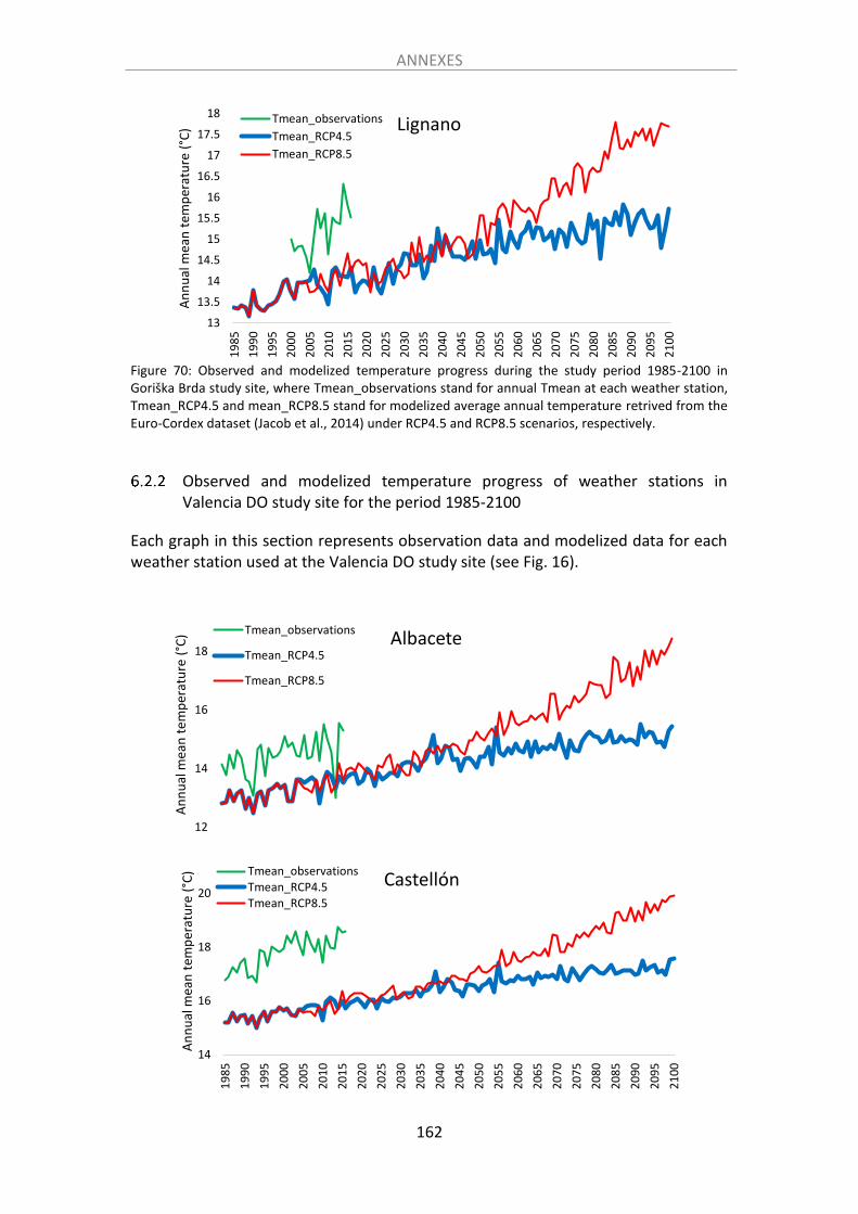
ANNEXES
162
Figure 70: Observed and modelized temperature progress during the study period 1985-2100 in Goriška Brda study site, where Tmean_observations stand for annual Tmean at each weather station, Tmean_RCP4.5 and mean_RCP8.5 stand for modelized average annual temperature retrived from the Euro-Cordex dataset (Jacob et al., 2014) under RCP4.5 and RCP8.5 scenarios, respectively.
Observed and modelized temperature progress of weather stations in Valencia DO study site for the period 1985-2100
Each graph in this section represents observation data and modelized data for each weather station used at the Valencia DO study site (see Fig. 16).
13
13.5
14
14.5
15
15.5
16
16.5
17
17.5
18
19
85
19
90
19
95
20
00
20
05
20
10
20
15
20
20
20
25
20
30
20
35
20
40
20
45
20
50
20
55
20
60
20
65
20
70
20
75
20
80
20
85
20
90
20
95
21
00
An
nu
al m
ean
tem
per
atu
re (
°C) LignanoTmean_observations
Tmean_RCP4.5
Tmean_RCP8.5
12
14
16
18
An
nu
al m
ean
tem
per
atu
re (
°C) Albacete
Tmean_observations
Tmean_RCP4.5
Tmean_RCP8.5
14
16
18
20
19
85
19
90
19
95
20
00
20
05
20
10
20
15
20
20
20
25
20
30
20
35
20
40
20
45
20
50
20
55
20
60
20
65
20
70
20
75
20
80
20
85
20
90
20
95
21
00
An
nu
al m
ean
tem
per
atu
re (
°C)
CastellónTmean_observationsTmean_RCP4.5Tmean_RCP8.5

ANNEXES
163
15
17
19
21
An
nu
al m
ean
tem
per
atu
re (
°C) ChesteTmean_observations
Tmean_RCP4.5
Tmean_RCP8.5
14
16
18
20
22
An
nu
al m
ean
tem
per
atu
re (
°C) LlíriaTmean_observations
Tmean_RCP4.5
Tmean_RCP8.5
11
13
15
17
19
19
85
19
89
19
93
19
97
20
01
20
05
20
09
20
13
20
17
20
21
20
25
20
29
20
33
20
37
20
41
20
45
20
49
20
53
20
57
20
61
20
65
20
69
20
73
20
77
20
81
20
85
20
89
20
93
20
97
An
nu
al m
ean
tem
per
atu
re (
°C) RequenaTmean_observations
Tmean_RCP4.5
Tmean_RCP8.5

ANNEXES
164
Figure 71: Observed and modelized temperature progress during the study period 1985-2100 at the Valencia DO study site, where Tmean_observations stand for annual Tmean at each weather station, Tmean_RCP4.5 and mean_RCP8.5 stand for modelized average annual temperature retrived from the Euro-Cordex dataset under RCP4.5 and RCP8.5 scenarios, respectively.
10
11
12
13
14
15
16
17
An
nu
al m
ean
tem
per
atu
re (
°C)
TeruelTmean_observations
Tmean_RCP4.5
Tmean_RCP8.5
16
17
18
19
20
21
22
19
85
19
90
19
95
20
00
20
05
20
10
20
15
20
20
20
25
20
30
20
35
20
40
20
45
20
50
20
55
20
60
20
65
20
70
20
75
20
80
20
85
20
90
20
95
21
00
An
nu
al m
ean
tem
per
atu
re (
°C)
Valenciaairport
Tmean_observations
Tmean_RCP4.5
Tmean_RCP8.5