Embed Size (px)
Citation preview
For Review O
nly
1
Spatially adapted total variation model to removemultiplicative noise
Dai-Qiang Chen, Li-Zhi Cheng
Abstract—Multiplicative noise removal based on total variation(TV) regularization has been widely researched in image science.This paper proposes a new variational model which combinesthe TV regularizer with local constraints. It is also related to aTV model with spatially adapted regularization parameters. Theautomated selection of the regularization parameters is based onthe local statistical characteristics of some random variable. Thecorresponding subproblem can be solved by the split Bregmanmethod efficiently. Numerical examples demonstrate that theproposed algorithm is able to preserve small image details whilethe noise in the homogeneous regions is removed sufficiently. Asa consequence, our method yields better denoised results thanthose of the recent state-of-the-art methods with respect to theSNR values.
Index Terms—total variation, Gamma noise, spatially adaptedregularization, split Bregman method.
I. INTRODUCTION
Image denoising is one of the widely researched problemsin image processing. For many special imaging systems suchas synthetic aperture radar (SAR), laser or ultrasound imaging,single particle emission computed tomography (SPECT) andpositron emission tomography (PET), image acquisition pro-cesses are different from the usual optical imaging technologyand the standard additive Gaussian noise model is not suitedin these situations. Instead, the multiplicative noise modelprovides an appropriate description of these special imagingsystems. For more details about the generation of multiplica-tive noise in above mentioned imaging acquisition processesrefer to [1, 2].
In this paper, we are interested in the problem of multiplica-tive noise removal. Assume Ω ⊂ R
2 is a rectangular domain.Let u(x) : Ω → R be the original image and f(x) ∈ L2(Ω)be the observed image corrupted with multiplicative noise; thedegradation model can be expressed as
f(x) = u(x)η(x), (1)
where the noise η is assumed to follow some distributionfor a special application, e.g., in synthetic aperture radar, ηfollows a Gamma distribution [2]; in ultrasound imaging, wemay also confront with Rayleigh distributed [3] or Riciandistributed noise [4]. Moreover, multiplicative Poisson noiseappears in various applications such as electronic microscopy,positron emission tomography and single photon emissioncomputerized tomography [5]. In this paper, we focus on
D.Q.Chen is with the Department of Mathematics, College of Science,National University of Defense and Technology, Changsha 410073, Hunan,People’s Republic of China e-mail: [email protected].
Gamma distributed noise and then η denotes Gamma noisewith density function:
Pη(z) =LL
Γ(L)zL−1e−Lz1{z≥0}. (2)
The mean of η is 1 and its standard deviation is 1√L
.Recently, various variational models and filter methods for
removing multiplicative noise were proposed. The first totalvariation (TV) approach to solve the multiplicative modelwas presented as Rudin-Lions-Osher model [6], which useda constrained optimization approach with two Lagrange mul-tipliers. However, their fitting term is not convex, whichleads to difficulties in using the iterative regularization orthe inverse scale space method. Later, Shi and Osher [7] uselogarithmic transformation on both side of (1) and convertthe multiplicative problem into the additive one. They thenextend the relaxed inverse scale space (RISS) flows to thetransformed additive problem. Numerical experiments showa good denoising effect and a significant improvement overearlier multiplicative models.
Derived from a MAP (maximum a posteriori) estimator,Aubert and Aujol [8] proposed a new total variation modelto remove multiplicative Gamma noise of images
minu∈BV (Ω)
∫Ω
|∇u|dx + μ
∫Ω
(log u +
f
u
)dx, (3)
where μ > 0 is a regularization parameter to control thetrade-off between the goodness-of-fit of f and a smoothnessrequirement due to the TV regularization. The TV regularizerTV(u) =
∫Ω|∇u|dx was first proposed by Rudin, Osher,
and Fatemi [9] for Gaussian noise removal. In the space offunctions of bounded variation (BV), the BV-seminorm isdefined by∫
Ω
|∇u| = sup{∫
Ω
u div�v dx : �v ∈ (C∞0 (Ω))2, ‖�v‖∞ ≤ 1
},
and u ∈ BV (Ω) iff
‖u‖BV (Ω) =∫
Ω
|∇u| + ‖u‖L1(Ω) < ∞.
The objective function in (3) is nonconvex, and hence thecomputed solution is sensitive to the initial value and is notnecessary to be a global optimal solution. Recently, in manyliteratures [7, 10, 11],
∫Ω|∇ log u| is used to replace the
regularizer∫Ω|∇u| in the problem (3). Note that∫
Ω
|∇ log u| = TV (log u) =∫
Ω
(|∇u|/u)
Page 29 of 54
123456789101112131415161718192021222324252627282930313233343536373839404142434445464748495051525354555657585960
For Review O
nly
2
is the well-known Weberized TV regularization term [12]. Theessential idea of it is the use of Weber’s law, which was firstdescribed in 1834 by German physiologist E.H.Weber [13].The law reveals the universal influence of the backgroundstimulus u > 0 on human sensitivity to the intensity incrementδu. Further, taking the rescaling w = log u, this results in aconvex minimization problem
minw∈BV (Ω)
∫Ω
|∇w|dx + μ
∫Ω
(w + fe−w
)dx, (4)
which overcomes the drawbacks of the AA model (3). Exper-iments show that this model outperforms the AA model [10,11].
Very recently, the equivalence of the problem (4) and I-divergence model
minu∈BV (Ω)
∫Ω
|∇u|dx + μ
∫Ω
(u − flogu) dx (5)
has been researched [14, 15]. Note that the problem (5) is theclassical model for Poisson noise removal. From [14, 15] weinfer that (5) is appropriate for multiplicative noise as well.
The TV regularizer appears in the above models is well-known for preserving sharp discontinuities, and hence becomeone of the standard techniques for image restoration. However,it may not generate good enough results for images withmany small structures and textures. The underlying causeof the problem is that only local features of the image areconsidered in the TV-based models. Recently, non-local (NL)filters [16-18] and variational models [19, 20] are developedfor deblurring and denoising of images. These methods areappropriate for capturing the fine structures within imagesand have been shown to be very efficient. However, thecomputational complexity is too high and they need muchmore time for execution.
In order to balance the quality and efficiency of imagerestoration, TV models with spatially adapted regularizationparameters were widely researched [21, 22]. We observe that,in the models (3)-(5), the value of μ controls the smoothness ofthe denoised image produced by the TV regularizer. Roughlyspeaking, small μ leads to over smoothing for small featuresin images so that fine details are removed; while large μleads to little smoothing and thus noise will remain almostunchanged in the homogeneous regions. Therefore, spatiallyadapted regularization parameters are more suitable for thedenoising problem. In [22], spatially varying constraints basedon local variance measures were proposed for Gaussian noiseremoval. The similar idea is also extended to deal withmultiplicative noise [23], where the proposed algorithm is toevolve the negative gradient flow based on the AA model andupdate the regularization parameters after each iteration. Sincethe proposed algorithm is an instance of the gradient descentmethod, it converges slowly and needs many iteration stepsfor good enough results. Moreover, since the AA model isnon-convex and the regularization parameter is varying alongthe iterative steps, there is no convergence results for thisalgorithm.
On the other hand, a new class of methods for automatedselection of the spatially adapted regularization parameters
depending on the local statistical characteristics of the noisewere developed for image denoising and deblurring [24-27].This results in a convex minimization problem which canbe solved efficiently by a superlinearly convergent algorithmbased on Fenchel-duality and inexact semismooth Newtontechniques. Moreover, the convergence properties of thesemethods are well established.
This paper discuss the local expected value estimator of arandom variable of the form
f
u− log
f
u, (6)
and deriving from this conclusion we propose a new TV modelwith local constraints for multiplicative noise removal. In thismodel, we use the Weberized TV regularizer instead of theTV regularizer, and by adopting the logarithm transform weobtain further a convex sub-minimization problem which canbe solved efficiently.
The rest of this paper is organized as follows. In sec-tion 2 we introduce the new locally constrained TV modelfor Gamma noise removal. In section 3 the existence anduniqueness of a solution to the proposed model are inves-tigated, and further we describe the relation between theconstrained problem and the corresponding TV model withspatially adapted regularization parameters. In section 4 weprovide a new spatially adapted algorithm which combinesan automated selection of the regularization parameters withthe split Bregman method for solving the corresponding sub-minimization problem. In section 4 we report the numericalresults comparing the proposed algorithm with those of therecent state-of-the-art methods.
II. CONSTRAINED TV MODEL FOR MULTIPLICATIVE NOISEREMOVAL
In this section, we first describe the statistical characteristicof some random variable with respect to Gamma noise η. Itplays an central role in developing our method in this section.
Proposition 1: Let η be a Gamma random variable (r.v)with mean 1 and standard deviation 1√
L. Consider the follow-
ing function of ηI(η) = η − log η. (7)
Then the following estimate of the expected value of I(η)holds true for large L:
E{I(η)} = 1 +1
2L+
112L2
− 52L3
+ O
(1L3
). (8)
Proof: We provide the proof in Appendix A.Next we study the property of the formula defined by (6).
Assume that a noise-free image is decomposed as follows:u = uc + ut, where uc > 0 and ut > 0 denote the cartoonpart and the texture part of the image, respectively. Thus f =(uc + ut) · η. Numerical Experiments demonstrate that TV-based model (3) and (4) can perform very well for cartoonimages (piecewise constant regions). Thus these models usingappropriate regularization parameter μ yield denoising resultssuch that u = uc. Under this assumption we have
f
u− log
f
u= η − log η +
{ut
ucη − log
(1 +
ut
uc
)}. (9)
Page 30 of 54
123456789101112131415161718192021222324252627282930313233343536373839404142434445464748495051525354555657585960
For Review O
nly
3
For the cartoon-like regions Ωc ⊂ Ω, we have ut ≈ 0, andthen according to (9) we obtain∫
Ωc
(f
u− log
f
u
)dx ≈
∫Ωc
(η − log η) dx ≈ E{I(η)} ≈ 1+ε
(10)where ε = 1
2L + 112L2 . For the image regions Ωt ⊂ Ω that
contain rich texture information, we have ut 0 and then by(9) we obtain∫
Ωt
(f
u− log
f
u
)dx >
∫Ωc
(η − log η) dx ≈ 1 + ε. (11)
Motivated by the above arguments, we can use the localexpected value estimator of f
u − log fu as a constrained con-
dition for the denoised image. Specifically, we define a localwindow centered at pixel x as follows:
Ωrx =
{y : ‖y − x‖∞ ≤ r
2
},
and assume that w(x, y) is the mean filter, i.e.
w(x, y) =
{1
|Ωrx| , if ‖y − x‖∞ ≤ r
2 ,
0, else.
Then the local expected value estimator can be defined asfollows:
F (u)(x) =∫
Ω
w(x, y)(
f
u− log
f
u
)(y)dy. (12)
Based on the formula (12) we obtain the following WeberizedTV minimization problem with local constraints
min∫
Ω
|∇ log u| over u ∈ BV (Ω)
s.t.F (u) ≤ 1 + ε a.e. in Ω,
(13)
where ’a.e.’ stands for ’almost everywhere’. Using the loga-rithm transform of the term z = log u, we get the equivalentTV minimization problem
min∫
Ω
|∇z| over z ∈ BV (Ω)
s.t.S(z) ≤ 1 + ε a.e. in Ω,
(14)
where
S(z)(x) = F (ez)(x) =∫
Ω
w(x, y)(fe−z + z − log f
)(y)dy.
(15)We observe that the function g(s) = s − log s ≥ 1 for anys > 0. Thus it is obvious that S(z)(x) ≥ 1 for any x ∈ Ω bychoosing s = fe−z .
For later use we define the feasible set of (14) as follows
C = {z ∈ BV (Ω) : S(z) ≤ 1 + ε a.e. in Ω}. (16)
Note that Ω is bounded and f ∈ L2(Ω), z ∈ BV (Ω). It issimple to show that fe−z + z − log f ∈ L1(Ω) and w ∈L∞(Ω×Ω). Thus we have S(z) ∈ L∞(Ω). Moreover, S(·) iscontinuous as a mapping from L2(Ω) to L∞(Ω). Therefore,it is straightforward to show that C is closed and convex.
III. SOME PROPERTIES OF THE PROPOSED TV MODEL
In this section, we address the problems of existence anduniqueness of a solution of the proposed model (14). Further,we observe that the constrained minimization problem (14) isrelated to a TV model with a spatially adapted regularizationparameter λ(x) ∈ L2(Ω) as follows:
minz∈BV (Ω)
∫Ω
|∇z|dx +∫
Ω
λ(z + fe−z
)dx. (17)
Based on this relationship, we propose a spatially adaptedTV algorithm for multiplicative noise removal, which will bedescribed in details next section.
In order to prove the existence of a solution to the problem(14), a technique similar to previous works [28] is adoptedhere. We first establish a BV-coercivity result for the function
L(z) = J(z) +∫
Ω
S(z)(x)dx
with J(z) =∫Ω|∇z|dx. Then the existence is a direct result.
Theorem 1: Assume fmin is a positive constant and f ≥fmin. Then ‖z‖BV → +∞ implies L(z) → +∞. Further, theproblem (14) admits a solution.
Proof: A sketch of the proof is given in Appendix B.Due to the convexity (only) of the problem, there is no
uniqueness result. However, if w(x, y) in (15) is replaced bya modified mean filter
w(x, y) =
{1
wr , if ‖y − x‖∞ ≤ r2 ,
ε0, else
where 0 < ε0 � min(1, 1
wr
)and wr satisfy∫
Ω
∫Ω
w(x, y)dxdy = 1. Then a uniqueness result can beestablished. For the proof refer to Appendix C.
Theorem 2: Let the assumptions of Theorem 1 hold true. Inaddition, we suppose that for any constant c, cχΩ ∈ C, whereχΩ(x) = 1 for x ∈ Ω. Then, the solution of the problem (14)is unique.
It is obvious that the condition cχΩ ∈ C is almost surelysatisfied when f is the product of some regular (non-constant)image and Gamma noise. Next we study the relation betweenthe problem (14) and (17). A technique based on the first-orderoptimality conditions is used in some previous works such asthe spatially adapted TV − Lτ (τ = 1, 2) models for impulseor Gaussian noise removal. This method can be extended tothe more general case and it is also suited for our problemhere. First, the following penalty problem is considered:
minLμ(z) = J(z) + μ
∫Ω
{max(S(z) − (1 + ε), 0)2
}dx
s.t. z ∈ BV (Ω),(18)
where μ > 0 denotes a penalty parameter. Then we have thefollowing result.
Theorem 3: Let the assumptions of Theorem 1 hold true.Then problem (18) admits a solution zμ ∈ BV (Ω) for everyμ > 0. Furthermore, for μ → +∞, {zμ} converges weakly
Page 31 of 54
123456789101112131415161718192021222324252627282930313233343536373839404142434445464748495051525354555657585960
For Review O
nly
4
along a subsequence in L2(Ω) to a solution of (14). Moreover,the formula
‖max(S(zμ) − 1 − ε, 0)‖L2(Ω) = o
(1√μ
)(19)
holds true, where limx→0 o(x)/x = 0 for any x ∈ R.Proof: Since similar proof appears in several papers [26,
27], we omit it here.Finally, we state the first-order optimality characterization
of a solution z of the problem (14), and this implies that z isalso a solution of the spatially adapted TV model (17) withcertain λ.
For subsequent results, we define
λ◦μ = μmax(S(zμ) − 1 − ε, 0), (20)
λμ =∫
Ω
w(x, y)λ◦μ(x)dx. (21)
Then we have
μ(‖max(S(zμ) − 1 − ε, 0)‖2L2(Ω)) =
∫Ω
λ◦μ(S(zμ) − 1 − ε)dx
=∫
Ω
λ◦μS(zμ)dx − Cμ =
∫Ω
λμqf (zμ)dx − Cμ,
(22)
where qf (s) = fe−s + s − log f and Cμ = (1 + ε)∫Ω
λ◦μdx.
Inspired by the formulas (18), (22) and the results inTheorem 3, we have the following result for the relation of(14) and (17).
Theorem 4: Let the assumptions of Theorem 1 hold true,and let z denote a weak limit point of {zμn
} as μn → +∞.Moreover, we assume that ‖zμn
‖L2(Ω) → ‖z‖L2(Ω) as μn →+∞, and that there exists C > 0 such that ‖λ◦
μn‖L1(Ω) ≤ C
for any n ∈ N. Then there exist λ ∈ L∞(Ω), a bounded Borelmeasure λ◦ and a subsequence {μnk
} such that the followingconclusions hold true:
(i)λμnkconverges weakly to λ in L∞(Ω), and λ ≥ 0 a.e.
in Ω.(ii)There exists j(z) ∈ ∂J(z) such that
〈j(z), q〉 +∫
Ω
λ(1 − fe−z
)qdx = 0, for all q ∈ BV (Ω).
(iii)∫Ω
ψλ◦μnk
→ ∫Ω
ψdλ◦ for all ψ ∈ C(Ω), and∫Ω
λ◦μn
(S(zμn) − 1 − ε)dx → 0.
Proof: The proof is similar to theorem 6 of [26], we omitit here.
Following Theorem 3 and Theorem 4(ii) we observe thatone solution of the constrained problem satisfies the first orderoptimality condition of (17) with λ = λ. Further, assume that(19) still holds with o(1/
√μ) replaced by o(1/μ). Then from
(20) we conclude that {λ◦μn
} is bounded in L2(Ω) and then λ◦
is the weak limit of a subsequence {λ◦μnk
}. If the last relationin Theorem 4(iii) holds as
∫Ω
λ◦(S(z) − 1 − ε)dx = 0, thenwe may equivalently write
λ◦ = λ◦ + δ max(S(z) − 1 − ε, 0), (23)
where δ > 0 is a fixed constant.Based on these results above an alternant iteration algorithm
is proposed in the next section.
IV. SPATIALLY ADAPTED ALGORITHM FORMULTIPLICATIVE NOISE REMOVAL
In this section, We focus on reconstructing an image suchthat the local constrained conditions in (14) hold in both thedetail regions and the homogeneous parts. From the discussionin section 3 we infer that it can be achieved by a suitableselection of the regularization parameter λ in the problem (17).
Inspired by [25-27], we adopt an adjustment strategy similarto the Lagrangian multiplier update for the parameter λ.Initially, we choose λ to be a small positive value, and thenobtain an over-smoothed restored image which keeps mostdetails in the residual. From section 2 we conclude thatS(z) > 1+ ε in the texture-rich image regions, which impliesthat λ needs to be increased there. Therefore, we propose theupdate rule of λ as follows: Assume λk denotes the currentestimate of λ◦ in Theorem 4. Then we set the update by
λk+1 = λk + δ max(S(zk) − 1 − ε, 0), (24)
λk+1 =∫
Ω
w(x, y)λk+1(x)dx, (25)
where δ > 0, and zk is the current estimate of the originallogarithmic image z. Note that (4.1)-(4.2) are motivated by(20)-(21) and (23).
Based on the update formulas in (24) and (25), we obtain thespatial adaptive TV algorithm for multiplicative noise removalshown as Algorithm 1. For the convenience of the discussionbelow, we present it in a discrete version.
Algorithm 1 Spatial adaptive TV algorithm for multiplicativenoise removal
Choose: noisy image f ; parameters λ0 and δ; localwindow size r;Initialization: k = 0, λk = λk = λ0;Iteration:
(1)Solve the discrete version of the problem
zk = arg minz∈BV (Ω)
{∫Ω
|∇z|dx +∫
Ω
λk(z + fe−z)dx
}by the method proposed in subsection 4.1.
(2)Based on zk, update λk as follows:
(λk+1)i,j = (λk)i,j + δ max(S(zk)i,j − 1 − ε, 0),
(λk+1)i,j =1r2
∑(s,t)∈Ωr
i,j
(λk+1)s,t.
(3)Stop, or set k = k + 1.
In the following, we make several remarks on the proposedalgorithm: (1)The initial value λ0 : the regularization param-eter λ in (17) controls the smoothness of the restored image.If λ is a scalar, it should satisfy the following relation:
λ ∝ 1/σ2 = L,
where σ2 is the variance of Gamma noise. Numerical examplesin section 5 demonstrate that the proportional relation aboveis also suitable for the setting of the initial value λ0.
Page 32 of 54
123456789101112131415161718192021222324252627282930313233343536373839404142434445464748495051525354555657585960
For Review O
nly
5
(2)The update step δ: it controls the change rate of λk andλk. Too small δ leads to a rather slow adjustment of λ; whiletoo large δ makes the algorithm unstable. We further study theinfluence of δ on the denoised results in the experiments nextsection, and observe that a proportional relation can also beestablished between δ and the variance of Gamma noise, i.eδ ∝ L. Moreover, for an appropriate value of δ, k = 3 or 4 isenough for Algorithm 1.
(3)The window size r: too small window size r should yieldobvious deviation between the local expected value estimatordefined by (12) and the theoretical value 1 + ε, which isa consequence of the small sample sizes; whereas too larger makes the regularization parameter choice becomes ratherglobal than local which compromises image details. In section5 we research the influence of different window sizes on therestoration quality.
(4)The algorithm for solving the spatially adapted TV modeldefined by (17): the augmented Lagrangian method [11, 29]can be used to solve (17) directly, but it will generate asub-minimization problem which needs to be solved by theNewton iteration method. Fortunately, based on the previousworks [14, 15] we could solve the I-divergence model (4) withμ = λ(x) ∈ L2(Ω) instead of it. For more details we refer tosection 4.1.
A. The augmented Lagrangian method for the spatiallyadapted TV model
First, we explain the relation of the spatially adapted TVmodel (17) and the I-divergence model
minu∈BV (Ω)
∫Ω
|∇u|dx +∫
Ω
λ (u − flogu) dx, (26)
which is given by the following result.Theorem 5: Assume 0 < λ0 ≤ λ(x) ≤ L for any x ∈ Ω,
where L is a positive constant. Let zλ and uλ denote thesolutions of (17) and (26) respectively. Then the followingrelation holds:
uλ = ezλ .
Proof: Let φ(x, s) .= λ(x)(s + f(x)e−s), ψ(x, s) .=λ(x)
(s + f(x) log f(x)
s + f(x))
and g(s) = es. Since 0 <
λ0 ≤ λ(x) ≤ L, it is obvious that the assumptions (B1)-(B2) [15] hold, and thus according to Theorem 8 of [15] weconclude that uλ = ezλ .
Next we describe the details of solving the I-divergencemodel (26) with the augmented Lagrangian method. Thediscrete version of the problem (26) is represented as
minu
TV (u) +n∑
i,j=1
λij (u − f log u)i,j . (27)
The isotropic discrete TV regularizer is defined by
TV (u) =n∑
i,j=1
√(Δh
iju)2 + (Δviju)2, (28)
where Δhiju and Δv
iju denote the horizontal and vertical firstorder differences at pixel (i, j); while the anisotropic discrete
TV regularizer is defined by the equation
TV (u) =n∑
i,j=1
|Δhiju| + |Δv
iju|. (29)
The proposed algorithm is based on the augmented La-grangian method. By introducing a new variable w we changethe problem (27) into a constrained minimization problem asfollows
minu,w
⎧⎨⎩TV (u) +
n∑i,j=1
λij (w − f log w)i,j |u = w
⎫⎬⎭ . (30)
The augmented Lagrangian function for (30) is defined by
Lηu,s = TV (u)+
n∑i,j=1
λij (w − f log w)i,j+〈s, u−w〉+η
2‖u−w‖2
2,
(31)where η is a positive penalty parameter and s is the Lagrangianmultiplier. We apply the so-called alternating direction methodof multipliers (ADMM) [29] to solve minLδ(u, s). Since thedetails are similar to related works such as those in [11, 30], weomit them and give the results shown as Algorithm 2 directly.
Algorithm 2 Augmented Lagrangian method for the spatiallyadapted TV model
Choose: image f ; regularization parameter λ; penaltyparameter η > 0; maximum iterative number K; toleranceerror ε > 0;Initialization: k = 0, uk = wk = f , bk=0;Iteration:
uk+1 = arg minu
{TV (u) + η
2‖u − (wk − bk)‖2}
;s = uk+1 + bk − λ
η ;
wk+1ij = 1
2 ×(sij +
√s2
ij + 4λijfij
η
);
bk+1 = bk + uk+1 − wk+1;k = k + 1;
until ‖uk+1−uk‖2‖uk‖2
< ε or k < K.
In each iteration of Algorithm 2, a ROF denoising problemis used to compute the value of uk. This problem can be solvedby Chambolles algorithm [31] or the split Bregman method[30]. Further, if we consider only one iteration of the splitBregman method for the ROF denoising problem in Algorithm2, then we obtain the corresponding augmented Lagrangianmethod for the following constrained minimization problem
minu,w,p
⎧⎨⎩‖p‖1 +
n∑i,j=1
λij (w − f log w)i,j |u = w, p = ∇u
⎫⎬⎭ ,
(32)where ‖p‖1 =
∑ni,j=1
√|p1
ij |2 + |p2ij |2 for isotropic total
variation and ‖p‖1 =∑n
i,j=1(|p1ij |+|p2
ij |) for anisotropic totalvariation. However, a reasonable amount of iterations for theROF denoising problem in Algorithm 2 is more efficient forobtaining a moderate accurate solution.
In the following experiments, we adopt the strategy of [11,section VI-A] for the running of Chambolles algorithm, i.e. ineach iteration of the proposed algorithm, the internal variables
Page 33 of 54
123456789101112131415161718192021222324252627282930313233343536373839404142434445464748495051525354555657585960
For Review O
nly
6
(a) (b)
(c) (d)
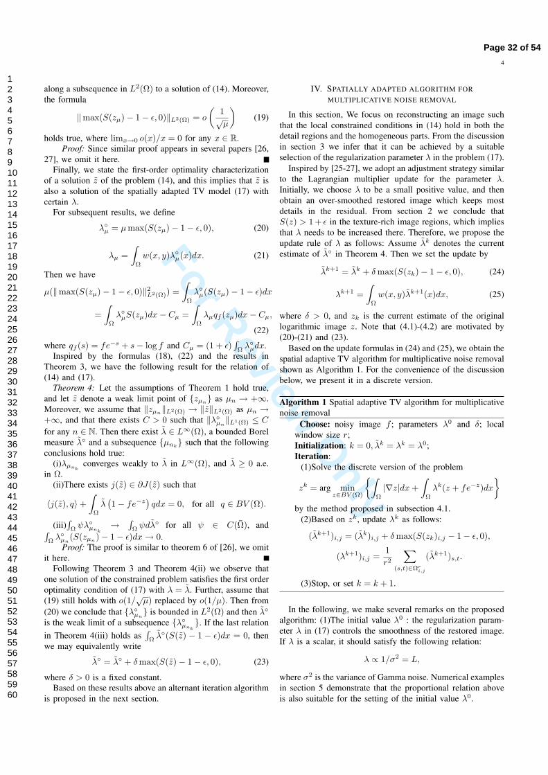
Fig. 1. Original images: (a)Lena, (b)Cameraman, (c)Barbara (d)Bars.
of Chambolles algorithm are initialized with those obtained inthe previous iteration. Thus a small number of iterations suchas K = 10 is needed for each call of Chambolles algorithm.
V. APPLICATION AND SIMULATED RESULTS
In this section, we make various experiments to evaluate theperformance of the proposed algorithm. First, the setting of theinitial regularization parameter λ0, window size r, and the stepparameter η in Algorithm 1 is researched; second, we comparethe performance of the proposed algorithm with those of therecent state-of-the-art methods introduced in [10, 11, 14],which solve the TV-based models with a scalar regularizationparameter; In the last part of experiments we compare our ap-proach with another recent state-of-the-art algorithm, proposedin [23], for which spatially varying regularization parametersare adopted and the solution is obtained by evolving thenegative gradient flow for the corresponding Euler-Lagrangeequation.
The code of Algorithm 1 are written entirely in Matlab, andall these algorithms are implemented under Windows XP andMATLAB 7.0 running on a Lenovo laptop with a Dual IntelPentium CPU 1.8G and 1 GB of memory. The four originalimages are shown in Fig. 1.
A. Parameters selection
In this subsection we focus on the study of the parametersselection in Algorithm 1. Two images called ’Lena’ and’Cameraman’ (see Figure 1) are used for our experiments. Foreach image, a noisy observation is generated by multiplyingthe original image by a realization of Gamma noise accordingto the formulas in (1)-(2) with L ∈ {8, 33}. The performanceof the proposed algorithm is measured quantitatively by means
1 2 3 4 5 69.5
10
10.5
11
11.5
12
12.5
iter num
PS
NR
(dB
) δ=5
δ=10
δ=20
δ=40
(a)
1 2 3 4 5 613.5
14
14.5
15
15.5
16
iter num
PS
NR
(dB
)
δ=5
δ=10
δ=20
δ=40
(b)
1 2 3 4 5 611
11.5
12
12.5
13
13.5
14
iter num
PS
NR
(dB
)
δ=2.5
δ=5
δ=10
δ=20
(c)
1 2 3 4 5 614.5
15
15.5
16
16.5
17
17.5
iter num
PS
NR
(dB
)
δ=5
δ=10
δ=20
δ=40
(d)
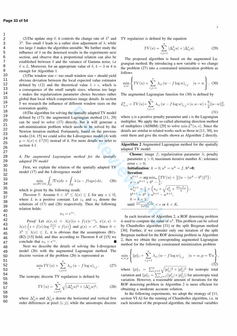
Fig. 2. Evolution of SNR along the iteration number of Algorithm 1 withdifferent δ: (a)Lena with L=8, (b)Lena with L=33, (c)Cameraman with L=8,(d)Cameraman with L=33.
of the signal-to-noise ratio (SNR), which is expressed as
SNR(u, g) = 10 lg{‖u − u‖2
‖g − u‖2
}, (33)
where u and g denote the original image and the restoredimage respectively, and u represents the mean of the originalimage. In each iteration of Algorithm 1, the sub-minimizationproblem (26) is solved by calling Algorithm 2. We chooseK = 15, ε = 10−3, and η = 0.15 for the running of Algorithm2.
In the following experiments, we study the influence ofvarious parameters in Algorithm 1 on the quality of thedenoised images.
Experiment 1 (the selection of the update step δ): ForAlgorithm 1, we observe that δ controls the change speed of λk
and hence has an important impact on the performance of thealgorithm. Specifically, large δ will lead to significant artifactsin image regions containing edges and details, especially forserious noise; while small δ makes the adjustment of λk
rather slow, which leads to an unacceptably large number ofiterations.
In this example, we fix λ0 = 0.1L and r = 17 for Algorithm1. Under these conditions, we plot the SNR values for thedenoised images with δ varying from 2.5 to 40 in Fig. 2.From the plots we observe that the values of SNR are ratherstable with respect to δ, unless δ is too large or too small. Wealso find that the optimum value of δ is inversely proportionalto the variance of Gamma noise, i.e.
δopt ≈ μ1L,
where μ1 is a positive constant. Moreover, we observe thatthe iteration number N = 3 or 4 is enough for the denoisedimages. Considering computational efficiency, we adopt N =3 in the experiments below.
Experiment 2 (the selection of the initial λ0): The reg-ularization parameter λk controls the trade-off between thegoodness-of-fit and the regularizer defined by the TV-norm. In
Page 34 of 54
123456789101112131415161718192021222324252627282930313233343536373839404142434445464748495051525354555657585960
For Review O
nly
7
0 0.1 0.2 0.3 0.412.5
13
13.5
14
14.5
15
15.5
16
16.5
μ2
PS
NR
(dB
)
L=8L=33
(a)
0 0.1 0.2 0.3 0.413.5
14
14.5
15
15.5
16
16.5
17
17.5
μ2
PS
NR
(dB
)
L=8L=33
(b)
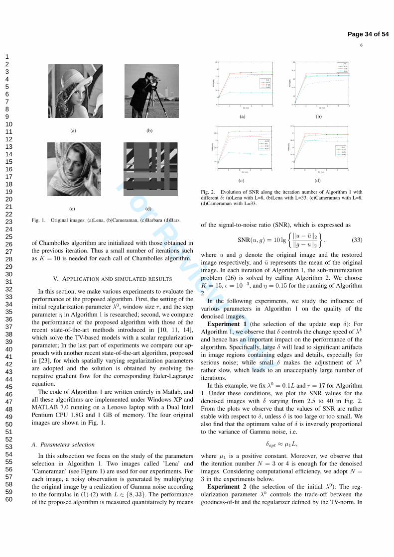
Fig. 3. SNR for images restored by Algorithm 1 with different initial μ2.(1.5dB is added to SNR values for image Lena and Cameraman with L=8respectively)
(a) (b)
(c) (d)
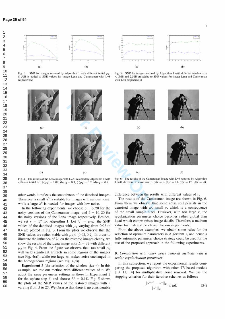
Fig. 4. The results of the Lena image with L=33 restored by Algorithm 1 withdifferent initial λ0. (a)μ2 = 0.02, (b)μ2 = 0.1, (c)μ2 = 0.2, (d)μ2 = 0.4.
other words, it reflects the smoothness of the denoised images.Therefore, a small λ0 is suitable for images with serious noise;while a large λ0 is needed for images with low noise.
In the following experiments, we choose δ = 5, 20 for thenoisy versions of the Cameraman image, and δ = 10, 20 forthe noisy versions of the Lena image respectively. Besides,we set r = 17 for Algorithm 1. Let λ0 = μ2L, the SNRvalues of the denoised images with μ2 varying from 0.02 to0.4 are plotted in Fig. 3. From the plots we observe that theSNR values are rather stable with μ2 ∈ [0.05, 0.2]. In order toillustrate the influence of λ0 on the restored images clearly, weshow the results of the Lena image with L = 33 with differentμ2 in Fig. 4. From the figure we observe that: too small μ2
will yield significant artifacts in some regions of the images(see Fig. 4(a)); while too large μ2 makes noise unchanged inthe homogeneous regions (see Fig. 4(d)).
Experiment 3 (the selection of the window size r): In thisexample, we test our method with different values of r. Weadopt the same parameter settings as those in Experiment 2for the update step δ, and choose λ0 = 0.1L. Fig. 5 showsthe plots of the SNR values of the restored images with rvarying from 5 to 25. We observe that there is no considerable
5 7 9 11 13 15 17 19 21 23 2514
14.2
14.4
14.6
14.8
15
15.2
15.4
15.6
15.8
16
r
PS
NR
(dB
)
L=8L=33
(a)
5 7 9 11 13 15 17 19 21 23 2515.5
16
16.5
17
17.5
r
PS
NR
(dB
)
L=8L=33
(b)
Fig. 5. SNR for images restored by Algorithm 1 with different window sizer. (3dB and 2.5dB are added to SNR values for image Lena and Cameramanwith L=8 respectively)
(a) (b)
(c) (d)
Fig. 6. The results of the Cameraman image with L=8 restored by Algorithm1 with different window size r. (a)r = 5, (b)r = 11, (c)r = 17, (d)r = 23.
difference between the results with different values of r.The results of the Cameraman image are shown in Fig. 6.
From them we observe that some noise still persists in thedenoised image with too small r, which is a consequenceof the small sample sizes. However, with too large r, theregularization parameter choice becomes rather global thanlocal which compromises image details. Therefore, a mediumvalue for r should be chosen for our experiments.
From the above examples, we obtain some rules for theselection of optimum parameters in Algorithm 1, and hence afully automatic parameter choice strategy could be used for thetest of the proposed approach in the following experiments.
B. Comparison with other noise removal methods with ascalar regularization parameter
In this subsection, we report the experimental results com-paring the proposed algorithm with other TV-based models[10, 11, 14] for multiplicative noise removal. We use thestopping criterion for their iterative schemes as follows
‖uk+1 − uk‖2
‖uk‖2< tol, (34)
Page 35 of 54
123456789101112131415161718192021222324252627282930313233343536373839404142434445464748495051525354555657585960
For Review O
nly
8
where uk denotes the iterate of the scheme. We set tol = 0.001for the following experiments.
In order to quantify the denoising performance, we list theSNR values of different denoised images by different methodsin Table 1. In this table, ”HNW”, ”MIDAL”, ”I-divergence”represent the Huang-Ng-Wen method in [10], multiplicativeimage denoising by the augmented Lagrangian method in [11],and the I-divergence-TV model in [14], respectively. Note thatthese methods are all manual parameter models. Among them,MIDAL and I-divergence require one regularization parameter;while HNW involves two input parameters: one parameteris for the regularization, and the other is for the closenessbetween the two denoised images. As in [10], we fix thecloseness parameter to be 19, and then we deal with onlyone parameter in the HNW method. In all these experiments,we adjust the regularization parameters of the three methodsto be optimal, in the sense that after many trials they yieldthe highest SNR denoising results. Meanwhile, we chooseδ ≈ 0.625L, λ0 = 0.1L, and r = 17 for Algorithm 1.From the table We observe that the proposed algorithm cangive better denoising results in terms of SNRs than othermethods. Quantitatively, we note that on average, 0.3 ∼ 0.6dBimprovement in SNR is obtained by our method.
TABLE ITHE VALUES OF SNR (DB) FOR DIFFERENT METHODS
Image L Noisy HNW MIDAL I-divergence Our method5 0.32 11.83 11.95 11.88 12.32
Cameraman 10 3.38 13.50 13.55 13.54 14.1325 7.33 15.74 15.67 15.58 16.395 -1.56 8.66 8.67 8.51 8.74
Barbara 10 1.42 9.66 9.65 9.73 10.1825 5.46 11.73 11.71 11.74 12.315 -0.22 11.79 11.82 11.78 12.25
Bars 10 2.69 13.68 13.70 13.83 14.2825 6.74 16.01 15.99 15.94 16.19
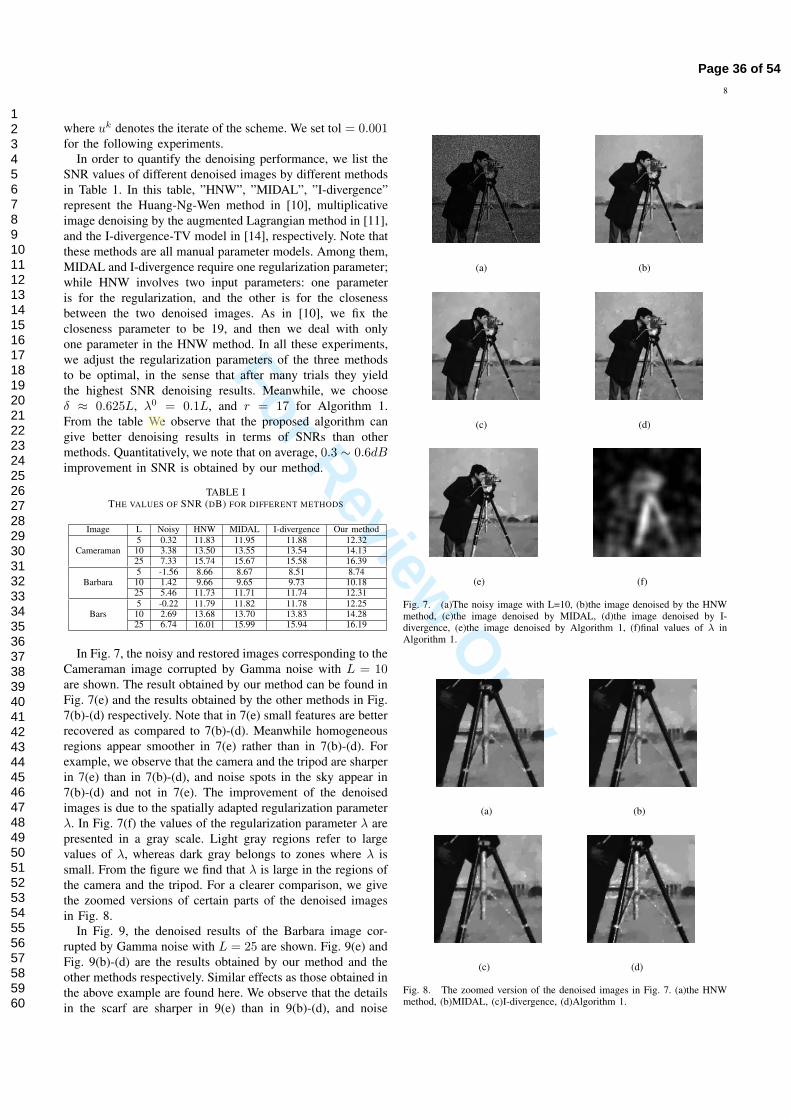
In Fig. 7, the noisy and restored images corresponding to theCameraman image corrupted by Gamma noise with L = 10are shown. The result obtained by our method can be found inFig. 7(e) and the results obtained by the other methods in Fig.7(b)-(d) respectively. Note that in 7(e) small features are betterrecovered as compared to 7(b)-(d). Meanwhile homogeneousregions appear smoother in 7(e) rather than in 7(b)-(d). Forexample, we observe that the camera and the tripod are sharperin 7(e) than in 7(b)-(d), and noise spots in the sky appear in7(b)-(d) and not in 7(e). The improvement of the denoisedimages is due to the spatially adapted regularization parameterλ. In Fig. 7(f) the values of the regularization parameter λ arepresented in a gray scale. Light gray regions refer to largevalues of λ, whereas dark gray belongs to zones where λ issmall. From the figure we find that λ is large in the regions ofthe camera and the tripod. For a clearer comparison, we givethe zoomed versions of certain parts of the denoised imagesin Fig. 8.
In Fig. 9, the denoised results of the Barbara image cor-rupted by Gamma noise with L = 25 are shown. Fig. 9(e) andFig. 9(b)-(d) are the results obtained by our method and theother methods respectively. Similar effects as those obtained inthe above example are found here. We observe that the detailsin the scarf are sharper in 9(e) than in 9(b)-(d), and noise
(a) (b)
(c) (d)
(e) (f)
Fig. 7. (a)The noisy image with L=10, (b)the image denoised by the HNWmethod, (c)the image denoised by MIDAL, (d)the image denoised by I-divergence, (e)the image denoised by Algorithm 1, (f)final values of λ inAlgorithm 1.
(a) (b)
(c) (d)
Fig. 8. The zoomed version of the denoised images in Fig. 7. (a)the HNWmethod, (b)MIDAL, (c)I-divergence, (d)Algorithm 1.
Page 36 of 54
123456789101112131415161718192021222324252627282930313233343536373839404142434445464748495051525354555657585960
For Review O
nly
9
(a) (b)
(c) (d)
(e) (f)
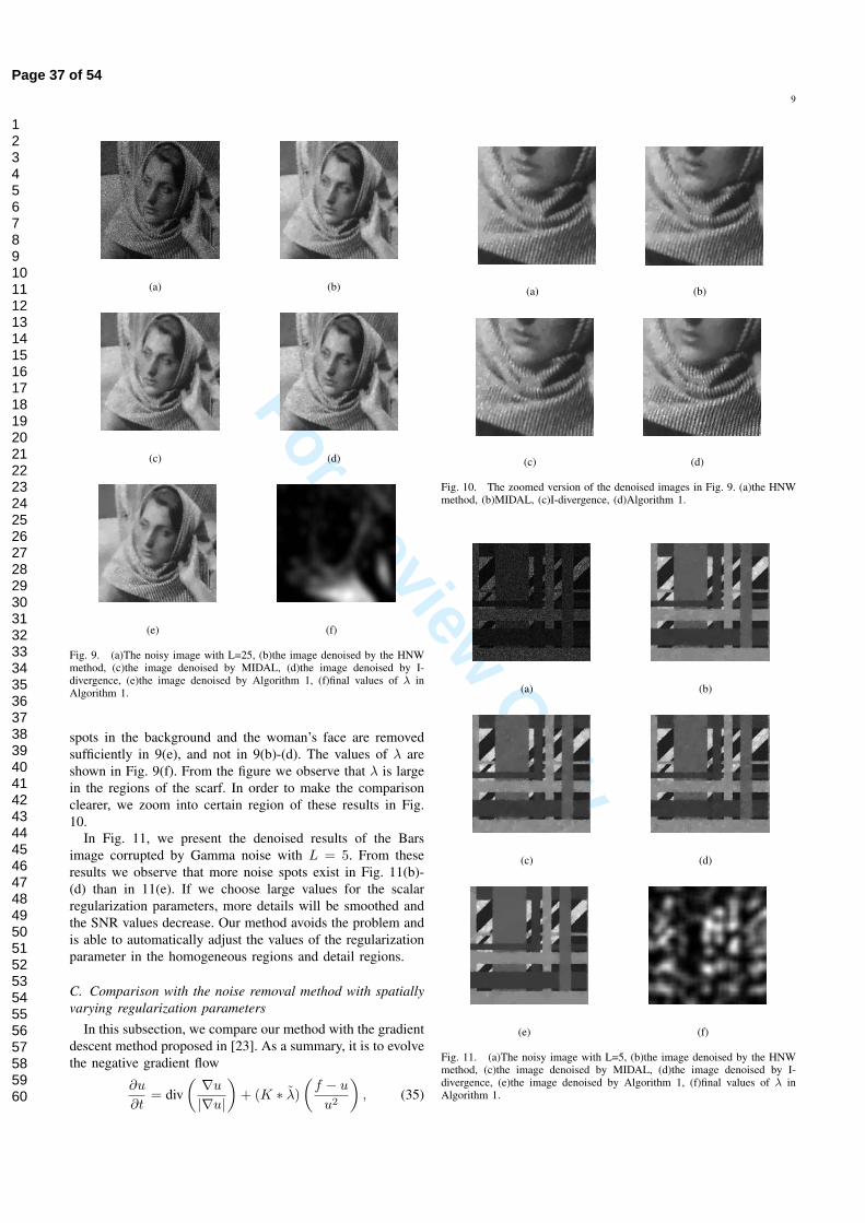
Fig. 9. (a)The noisy image with L=25, (b)the image denoised by the HNWmethod, (c)the image denoised by MIDAL, (d)the image denoised by I-divergence, (e)the image denoised by Algorithm 1, (f)final values of λ inAlgorithm 1.
spots in the background and the woman’s face are removedsufficiently in 9(e), and not in 9(b)-(d). The values of λ areshown in Fig. 9(f). From the figure we observe that λ is largein the regions of the scarf. In order to make the comparisonclearer, we zoom into certain region of these results in Fig.10.
In Fig. 11, we present the denoised results of the Barsimage corrupted by Gamma noise with L = 5. From theseresults we observe that more noise spots exist in Fig. 11(b)-(d) than in 11(e). If we choose large values for the scalarregularization parameters, more details will be smoothed andthe SNR values decrease. Our method avoids the problem andis able to automatically adjust the values of the regularizationparameter in the homogeneous regions and detail regions.
C. Comparison with the noise removal method with spatiallyvarying regularization parameters
In this subsection, we compare our method with the gradientdescent method proposed in [23]. As a summary, it is to evolvethe negative gradient flow
∂u
∂t= div
( ∇u
|∇u|)
+ (K ∗ λ)(
f − u
u2
), (35)
(a) (b)
(c) (d)
Fig. 10. The zoomed version of the denoised images in Fig. 9. (a)the HNWmethod, (b)MIDAL, (c)I-divergence, (d)Algorithm 1.
(a) (b)
(c) (d)
(e) (f)
Fig. 11. (a)The noisy image with L=5, (b)the image denoised by the HNWmethod, (c)the image denoised by MIDAL, (d)the image denoised by I-divergence, (e)the image denoised by Algorithm 1, (f)final values of λ inAlgorithm 1.
Page 37 of 54
123456789101112131415161718192021222324252627282930313233343536373839404142434445464748495051525354555657585960
For Review O
nly
10
where K is a two-dimensional Gaussian kernel, and λ isupdated by
λ(x) =D(x)V (x)
, x ∈ Ω. (36)
In the formula (36), D(x) = div(
∇u|∇u|
)(u− f), and V (x) ≈
σ4
K∗(r−r)2 , where r = fu − 1, r is the local mean of r, and u
is an approximation of the original image. This algorithm isinefficient for the noise removal especially when the noise isserious. In this case, we must choose a small iteration step toensure convergence of the algorithm, and hence thousands ofiteration steps are needed for good enough results. Therefore,we only consider the case of low noise here. For the gradientdescent method, we use the stopping criterion that the meanvalue of |uk−uk−1| should be less than 0.01, where uk denotesthe iterate of the scheme. Besides, the window size is set tobe 17, and the iteration step is set to be 0.2.
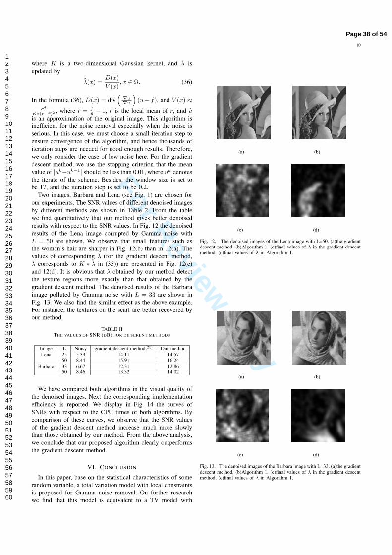
Two images, Barbara and Lena (see Fig. 1) are chosen forour experiments. The SNR values of different denoised imagesby different methods are shown in Table 2. From the tablewe find quantitatively that our method gives better denoisedresults with respect to the SNR values. In Fig. 12 the denoisedresults of the Lena image corrupted by Gamma noise withL = 50 are shown. We observe that small features such asthe woman’s hair are sharper in Fig. 12(b) than in 12(a). Thevalues of corresponding λ (for the gradient descent method,λ corresponds to K ∗ λ in (35)) are presented in Fig. 12(c)and 12(d). It is obvious that λ obtained by our method detectthe texture regions more exactly than that obtained by thegradient descent method. The denoised results of the Barbaraimage polluted by Gamma noise with L = 33 are shown inFig. 13. We also find the similar effect as the above example.For instance, the textures on the scarf are better recovered byour method.
TABLE IITHE VALUES OF SNR (DB) FOR DIFFERENT METHODS
Image L Noisy gradient descent method[23] Our methodLena 25 5.39 14.11 14.57
50 8.44 15.91 16.24Barbara 33 6.67 12.31 12.86
50 8.46 13.32 14.02
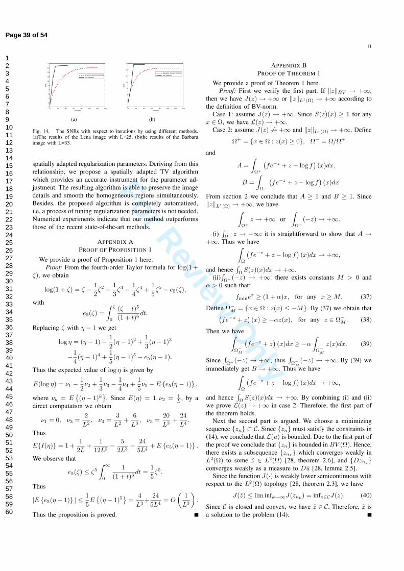
We have compared both algorithms in the visual quality ofthe denoised images. Next the corresponding implementationefficiency is reported. We display in Fig. 14 the curves ofSNRs with respect to the CPU times of both algorithms. Bycomparison of these curves, we observe that the SNR valuesof the gradient descent method increase much more slowlythan those obtained by our method. From the above analysis,we conclude that our proposed algorithm clearly outperformsthe gradient descent method.
VI. CONCLUSION
In this paper, base on the statistical characteristics of somerandom variable, a total variation model with local constraintsis proposed for Gamma noise removal. On further researchwe find that this model is equivalent to a TV model with
(a) (b)
(c) (d)
Fig. 12. The denoised images of the Lena image with L=50. (a)the gradientdescent method, (b)Algorithm 1, (c)final values of λ in the gradient descentmethod, (c)final values of λ in Algorithm 1.
(a) (b)
(c) (d)
Fig. 13. The denoised images of the Barbara image with L=33. (a)the gradientdescent method, (b)Algorithm 1, (c)final values of λ in the gradient descentmethod, (c)final values of λ in Algorithm 1.
Page 38 of 54
123456789101112131415161718192021222324252627282930313233343536373839404142434445464748495051525354555657585960
For Review O
nly
11
0 20 40 60 80 100 120 1405
6
7
8
9
10
11
12
13
14
15
seconds
SN
R
gradient descent method our method
(a)
0 20 40 60 80 100 120 1406
7
8
9
10
11
12
13
seconds
SN
R
gradient descent method our method
(b)
Fig. 14. The SNRs with respect to iterations by using different methods.(a)The results of the Lena image with L=25, (b)the results of the Barbaraimage with L=33.
spatially adapted regularization parameters. Deriving from thisrelationship, we propose a spatially adapted TV algorithmwhich provides an accurate instrument for the parameter ad-justment. The resulting algorithm is able to preserve the imagedetails and smooth the homogeneous regions simultaneously.Besides, the proposed algorithm is completely automatized,i.e. a process of tuning regularization parameters is not needed.Numerical experiments indicate that our method outperformsthose of the recent state-of-the-art methods.
APPENDIX APROOF OF PROPOSITION 1
We provide a proof of Proposition 1 here.Proof: From the fourth-order Taylor formula for log(1 +
ζ), we obtain
log(1 + ζ) = ζ − 12ζ2 +
13ζ3 − 1
4ζ4 +
15ζ5 − e5(ζ),
with
e5(ζ) =∫ ζ
0
(ζ − t)5
(1 + t)6dt.
Replacing ζ with η − 1 we get
log η = (η − 1) − 12(η − 1)2 +
13(η − 1)3
−14(η − 1)4 +
15(η − 1)5 − e5(η − 1).
Thus the expected value of log η is given by
E(log η) = ν1 − 12ν2 +
13ν3 − 1
4ν4 +
15ν5 − E {e5(η − 1)} ,
where νk = E{(η − 1)k
}. Since E(η) = 1, ν2 = 1
L , by adirect computation we obtain
ν1 = 0, ν3 =2L2
, ν4 =3L2
+6L3
, ν5 =20L3
+24L4
.
Thus
E{I(η)} = 1 +1
2L+
112L2
− 52L3
− 245L4
+ E {e5(η − 1)} .
We observe that
e5(ζ) ≤ ζ5
∫ ∞
0
1(1 + t)6
dt =15ζ5.
Thus
|E {e5(η − 1)} | ≤ 15E
{(η − 1)5
}=
4L3
+245L4
= O
(1L3
).
Thus the proposition is proved.
APPENDIX BPROOF OF THEOREM 1
We provide a proof of Theorem 1 here.Proof: First we verify the first part. If ‖z‖BV → +∞,
then we have J(z) → +∞ or ‖z‖L1(Ω) → +∞ according tothe definition of BV-norm.
Case 1: assume J(z) → +∞. Since S(z)(x) ≥ 1 for anyx ∈ Ω, we have L(z) → +∞.
Case 2: assume J(z) → +∞ and ‖z‖L1(Ω) → +∞. Define
Ω+ = {x ∈ Ω : z(x) ≥ 0}, Ω− = Ω/Ω+
and
A =∫
Ω+
(fe−z + z − log f
)(x)dx,
B =∫
Ω−
(fe−z + z − log f
)(x)dx.
From section 2 we conclude that A ≥ 1 and B ≥ 1. Since‖z‖L1(Ω) → +∞, we have∫
Ω+z → +∞ or
∫Ω−
(−z) → +∞.
(i)∫Ω+ z → +∞: it is straightforward to show that A →
+∞. Thus we have∫Ω
(fe−z + z − log f
)(x)dx → +∞,
and hence∫Ω
S(z)(x)dx → +∞.(ii)
∫Ω−(−z) → +∞: there exists constants M > 0 and
α > 0 such that:
fminex ≥ (1 + α)x, for any x ≥ M. (37)
Define Ω−M = {x ∈ Ω : z(x) ≤ −M}. By (37) we obtain that(
fe−z + z)(x) ≥ −αz(x), for any z ∈ Ω−
M . (38)
Then we have∫Ω−
M
(fe−z + z
)(x)dx ≥ −α
∫Ω−
M
z(x)dx. (39)
Since∫Ω−(−z) → +∞, thus
∫Ω−
M(−z) → +∞. By (39) we
immediately get B → +∞. Thus we have∫Ω
(fe−z + z − log f
)(x)dx → +∞,
and hence∫Ω
S(z)(x)dx → +∞. By combining (i) and (ii)we prove L(z) → +∞ in case 2. Therefore, the first part ofthe theorem holds.
Next the second part is argued. We choose a minimizingsequence {zn} ⊂ C. Since {zn} must satisfy the constraints in(14), we conclude that L(u) is bounded. Due to the first part ofthe proof we conclude that {zn} is bounded in BV (Ω). Hence,there exists a subsequence {znk
} which converges weakly inL2(Ω) to some z ∈ L2(Ω) [28, theorem 2.6], and {Dznk
}converges weakly as a measure to Du [28, lemma 2.5].
Since the function J(·) is weakly lower semicontinuous withrespect to the L2(Ω) topology [28, theorem 2.3], we have
J(z) ≤ lim infk→∞J(znk) = infz∈CJ(z). (40)
Since C is closed and convex, we have z ∈ C. Therefore, z isa solution to the problem (14).
Page 39 of 54
123456789101112131415161718192021222324252627282930313233343536373839404142434445464748495051525354555657585960
For Review O
nly
12
APPENDIX CPROOF OF THEOREM 2
We provide a proof of Theorem 2 here.Proof: Let qf (s) = fe−s + s − log f . Since f > 0, it
is obvious that qf (s) is strictly convex. Let z1, z2 ∈ BV (Ω)denote two solutions of (14) with z1 = z2. Define z = 1
2 (z1 +z2). By the convexity of qf (s) we have
qf (z) ≤ 12(qf (z1) + qf (z2)). (41)
If the inequality holds as an equality a.e. in Ω, then by thestrictly convexity of qf (s) we obtain that z1 = z2 a.e. in Ω;otherwise there exist δ > 0 and Ωδ ⊂ Ω with |Ωδ| > 0 suchthat
qf (z) ≤ 12(qf (z1) + qf (z2)) − δ a.e. in Ωδ. (42)
Define εδ = ε0δ|Ωδ|. According to the formula (15) withw(x, y) = w(x, y) we get
S(z)(x) ≤ 12(S(z1)(x)+S(z2)(x))−εδ ≤ 1+ε−εδ a.e. in Ω.
(43)Define zθ = θz for θ ∈ [0, 1]. Since S(·) is continuous, thenfor θ close to 1, we have zθ ∈ C. Moreover, J(zθ) = θJ(z) <J(z) for any θ ∈ [0, 1), except J(z) = 0. This implies z ≡cχΩ for some c ∈ R. However, this is impossible since cχΩ ∈C. Hence, z1 = z2 a.e. in Ω.
REFERENCES
[1] J. Goodman, Speckle Phenomena in Optics: Theory and Applications,Roberts and Company Publishers, 2007.
[2] C. Oliver and S. Quegan, Understanding Synthetic Aperture RadarImages, Artech House, 1998.
[3] R. F. Wagner, S. W. Smith, and J. M. Sandrik, Statistics of speckle inultrasound B-scans, IEEE Trans. on Sonics Ultrason., 30(3) (1983)156-163.
[4] M. F. Isana, R. F. Wagner, B. S. Garra, D. G. Brown, and T. H. Shawker,Analysis of ultrasound image texture via generalized rician statistics, Opt.Eng., 25(6) (1986) 743-748.
[5] G. T. Herman, Fundamentals of Computerized Tomography: Image Re-construction from Projections, 2nd ed., Springer, ISBN 978-1-85233-617-2, 2009.
[6] L. I. Rudin, P.-L. Lions, and S. Osher, Multiplicative denoising anddeblurring: theory and algorithms, Chapter 6 in: Geometric Level SetMethods in Imaging, Vision, and Graphics, S. Osher and N. Paragios,Eds. pp. 103-120, Springer-Verlag, New York 2003.
[7] J. Shi and S. Osher, A nonlinear inverse scale space method for a convexmultiplicative noise model, SIAM J. Imaging Sci., 1(3) (2008) 294-321.
[8] G. Aubert and J. Aujol, A variational approach to remove multiplicativenoise, SIAM J. Appl. Math., 68 (2008) 925-946.
[9] L. Rudin, S. Osher, and E. Fatemi, Nonlinear total variation based noiseremoval algorithms, Physica D, 60 (1992) 259-268.
[10] Y. Huang, M. Ng, and Y. Wen, A new toal variation method formultiplicative noise removal, SIAM J. Imaging Sci., 2(1) (2009) 20-40.
[11] J.M. Bioucas-Dias, M.A.T. Figueiredo, Multiplicative Noise RemovalUsing Variable Splitting and Constrained Optimization, IEEE Trans.Image Process., 19(7) (2010) 1720-1730.
[12] J.H.Shen, On the foundations of vision modeling: I. Weber’s law andWeberized TV restoration, Physica D: Nonlinear Phenomena, 175 (3/4)(2003) 241-251.
[13] E. H. Weber, De pulsu, resorptione, audita et tactu, in Annotationesanatomicae et physiologicae, Koehler, Leipzig, Germany, 1834.
[14] G. Steidl, T. Teuber, Removing multiplicative noise by Douglas-Rachford splitting methods, J. Math. Imaging Vis., 36(2)(2010) 168-184.
[15] M. Grasmair, A coarea formula for anisotropic total variation regulari-sation, Preprint to appear, University of Vienna (2009).
[16] A. Buades, B. Coll, and J. Morel, A Non-Local Algorithm for ImageDenoising, IEEE Computer Society Conference on Computer Vision andPattern Recognition, vol. 2, 2005.
[17] C. Kervrann, P. Perez, and J. Boulanger, Bayesian non-local means,image redundancy and adaptive estimation for image representation andapplications, in SIAM Conf. on Imaging Science, San Diego, CA, July2008.
[18] Charles-Alban Deledalle , Loıc Denis , Florence Tupin, Iterativeweighted maximum likelihood denoising with probabilistic patch-basedweights, IEEE Trans. Image Process., 18(12) (2009) 2661-2672.
[19] S. Kindermann, S. Osher, and P. W. Jones, Deblurring and denoisingof images by nonlocal functionals, SIAM Multiscale Model. Simul. 4(4)(2005) 1091-1115.
[20] D.Q.Chen, H.Zhang, L.Z.Cheng, Nonlocal variational model and filteralgorithm to remove multiplicative noise, Opt. Eng., 49(07) (2010)077002.
[21] M. Grasmair, Locally adaptive total variation regularization, In SSVM’09: Proceedings of the Second International Conference on Scale Spaceand Variational Methods in Computer Vision, pp. 331-342, Berlin, Hei-delberg, 2009. Springer-Verlag, ISBN 978-3-642-02255-5.
[22] G. Gilboa, N. Sochen, and Y. Y. Zeevi, Variational denoising of partlytextured images by spatially varying constraints, IEEE Trans. ImageProcess., 15 (2006) 2281-2289.
[23] F. Li, M. Ng and C.M. Shen, Multiplicative noise removal with spatial-varying regularization parameters, SIAM J. Imaging Sci. 3(1) (2010) 1-20.
[24] M. Bertalmio, V. Caselles, B. Rouge, and A. Sole, TV based imagerestoration with local constraints, J. Sci. Comput. 19 (2003) 95-122.
[25] A. Almansa, C. Ballester, V. Caselles, and G. Haro, A TV basedrestoration model with local constraints, J. Sci. Comput. 34(3) (2008)209-236.
[26] Y. Q. Dong, M. Hintermuller and M. M. Rincon-Camacho, AutomatedRegularization Parameter Selection in Multi-Scale Variation Models forImage Restoration, J. Math. Imaging Vis., 40(1) (2011) 82-104.
[27] M. Hintermuller and M. M. Rincon-Camacho, Expected Absolute ValueEstimators for a Spatially Adapted Regularization Parameter Choice Rulein L1-TV-Based Image Restoration, Inverse Problems 26 (2010) 085005.
[28] R.Acar and C. R. Vogel, Analysis of bounded variation penalty methodsfor ill-posed problems, Inverse Problems 10 (1994) 1217-29.
[29] J. Eckstein, D. Bertsekas, On the Douglas-Rachford splitting methodand the proximal point algorithm for maximal monotone operators,Mathematical Programming, 55(3) (1992) 293-318.
[30] M. Figueiredo, J. Bioucas-Dias, Restoration of Poissonian images usingalternating direction optimization, IEEE Trans. Image Process, 19(12)(2010) 3133 - 3145.
[31] A. Chambolle, An algorithm for total variation minimization and appli-cations, J. Math. Imaging Vis., 20 (2004) 89-97.
Page 40 of 54
123456789101112131415161718192021222324252627282930313233343536373839404142434445464748495051525354555657585960