Embed Size (px)
Citation preview

192 J. Opt. Soc. Am. A/Vol. 14, No. 1 /January 1997 D. A. Boas and A. G. Yodh
Spatially varying dynamical properties of turbidmedia probed with
diffusing temporal light correlation
D. A. Boas* and A. G. Yodh
Department of Physics, University of Pennsylvania, Philadelphia, Pennsylvania 19104
Received June 21, 1996; accepted August 26, 1996; revised September 16, 1996
The diffusion of correlation is used to detect, localize, and characterize dynamical and optical spatial inhomo-geneities in turbid media and is accurately modeled by a correlation diffusion equation. We demonstrate ex-perimentally and with Monte Carlo simulations that the transport of correlation can be viewed as a correlationwave $analogous to a diffuse photon-density wave [Phys. Today 48, 34 (1995)]% that propagates spherically out-ward from sources and scatters from macroscopic spatial variations in dynamical and/or optical properties.We demonstrate the utility of inverse scattering algorithms for reconstructing images of the spatially varyingdynamical properties of turbid media. The biomedical applicability of this diffuse correlation probe is illus-trated in studies of the depth of burned tissues. © 1997 Optical Society of America. [S0740-3232(97)02301-6]
1. INTRODUCTIONThe potential to acquire information about tissue opticaland dynamical properties noninvasively offers excitingpossibilities for medical imaging. For this reason, thediffusion of near-infrared photons in turbid media hasbeen the focus of substantial recent research.1–4 Appli-cations range from pulse oximetry5–10 to tissuecharacterization11,12 to imaging of breast and braintumors13–15 to probing blood flow.16–19
When a photon scatters from a moving particle its car-rier frequency is Doppler shifted by an amount propor-tional to the speed of the scattering particle and is depen-dent on the scattering angle relative to the velocity of thescatterer. Measurements of the small frequency shiftscaused by Doppler scattering events make possible thenoninvasive study of particle motions and density fluctua-tions in a wide range of systems, such as the Brownianmotion of suspended macromolecules,20–23 velocimetry offlow fields,24–27 and in vivo blood flow monitoring.28–30
The methods for using light to study motions by meansof speckle fluctuations have appeared with numerousnames over the years.22,23,31–35 In most of these intensityfluctuation or light-beating measurements the quantity ofinterest is the electric-field temporal autocorrelation func-tion G1(r, t) 5 ^E(r, t)E* (r, t 1 t)& or its Fouriertransform I(r, v). Here the angle brackets ^ & denote en-semble averages (or averages over time t for most systemsof practical interest), r represents the position of the de-tector, and t is the correlation time. Both methodologiesare sensitive and useful.36 In most practical situationsone measures a light-intensity temporal correlation func-tion or Fourier equivalent and then applies the Bloch–Siegert relation32,34,37 to deduce the field correlation func-tions or Fourier equivalent. The field correlationfunction is explicitly related to the motions within thesample under study. Since our theoretical formulationand measurements have generally focused on the time-
0740-3232/97/010192-24$10.00 ©
domain picture,38–40 we shall continue to adopt that pic-ture throughout this paper. We note, however, that aline-shape analysis of the light spectrum obtained by thefrequency-domain instruments will provide entirelyequivalent information.The photon correlation methods and Fourier equiva-
lents have been used with great success in optically thinsamples. More recently there has been a greater effort toquantify this class of signal from turbid samples. For ex-ample, the development and the application of diffusing-wave spectroscopy (DWS),32–35 whereby temporal correla-tions of highly scattered light probe dynamical motions inhomogeneous complex fluids such as colloids,41–47
foams,48,49 emulsions,50 and gels.51 In the medical com-munity application of the theory of Bonner and Nossal30
has led to a better accounting of the spectral broadeningof a light field as it travels through a highly scatteringmedia while experiencing some scattering events fromstationary scatterers and some from moving cells.Recently we have developed and applied a formalism
for the treatment of light fluctuation transport in hetero-geneous highly scattering media. We have introduced adiffusion equation for the migration of the electric-fieldtemporal autocorrelation function through turbidmedia.38 The so-called correlation diffusion equation is ageneralization of the photon diffusion equation that en-compasses the well-known propagation of diffuse photon-density waves1; however, it also provides a mathematicaldescription that accounts for the effects of motional fluc-tuations on the spectrum (or the temporal correlations) ofpropagating diffusive waves. The equation includes theeffects of absorption, scattering, and dynamical motions.Importantly, it provides a natural framework when one isconsidering turbid media with spatially varying proper-ties. The new approach is formally similar to much ofthe research being carried out in the photon migrationcommunity.1–4 Thus it will be possible to empower many
1997 Optical Society of America

D. A. Boas and A. G. Yodh Vol. 14, No. 1 /January 1997 /J. Opt. Soc. Am. A 193
of the technical advances already made toward functionalimaging and spectroscopy with diffusing light, and it willbe possible to integrate a qualitatively new technologyinto existing optical instrumentation.In this paper we have attempted to develop thoroughly
and to apply ideas that we have presented in earlierpapers.38,40 The paper is organized as follows. Section 2reviews the theory of photon correlation spectroscopyfrom the single-scattering regime to the multiple-scattering regime. Section 3 describes the setup for ourexperimental measurements and the approach for ourMonte Carlo simulations. The experimental and thesimulation results are discussed in Sections 4 and 5, re-spectively. Section 6 demonstrates, with an animalmodel, that tissue burns varying in depth by 100 mm canbe distinguished. A summary is given in Section 7,which is followed by a detailed derivation, given in Ap-pendix A, of the correlation diffusion equation from thecorrelation transport equation.
2. THEORYWhen a beam of laser light with uniform intensity mi-grates through a turbid sample, the emerging intensitypattern is not uniform but will instead be composed ofmany bright and dark spots called speckles. The varia-tions arise because the photons that emerge from thesample have traveled along different paths that interfereconstructively and destructively at different detector po-sitions. If the scattering particles in the turbid mediumare moving, the speckle pattern will fluctuate in time.For the turbid medium, the time scale of the speckle in-
tensity fluctuations depends on the number of interac-tions that detected photons have had with moving scat-tering particles. In this section we briefly review thetheory for temporal field autocorrelation functions of lightscattered from optically dilute systems, i.e., photons scat-
ter no more than once before being detected. We thendiscuss the extension of single-scattering theory to sys-tems that multiply scatter light. After a brief review ofDWS, we describe in detail a new and general descriptionbased on the transport of correlation in optically densesystems.
A. Single ScatteringConsider the system depicted in Fig. 1. A beam of coher-ent light is incident upon a dilute suspension of identicalscattering particles. The light scattered by an angle u isdetected by a photodetector. The electric field reachingthe detector is a superposition of all the scattered electricfields:
E 5 EoF~q !(n51
N
exp~ikin • rn!exp@ikout • ~Rd 2 rn!#
5 EoF~q !exp~ikout • Rd!(n51
N
exp~2iq • rn!. (1)
Here E is the electric field reaching the detector at posi-tion Rd , Eo is the amplitude of the incident field, andF(q) is the form factor for light to receive a momentumtransfer of q 5 kout 2 kin , where kout and kin are the out-put and the input wave vectors, respectively, and uqu5 2ko sin u/2, with ko 5 uk inu 5 ukoutu. For simplicitywe neglect polarization effects and assume randomly po-sitioned and oriented scatterers. Under these conditionsthe differential scattering cross section is dependent onlyon the magnitude of q. The summation is over the Nparticles in the scattering volume, and rn is the positionof each particle. We can see from Eq. (1) that the phaseof each scattered wave depends on the momentum trans-fer (i.e., scattering angle) and on the position of the par-ticle. In a disordered system the particles are randomlydistributed, resulting in random constructive and de-
Fig. 1. Schematic of system in which light is incident upon a dilute suspension of scatterers. The suspension is dilute enough thatphotons are scattered no more than once. Scattered light is measured at an angle u defined by two pinholes and is monitored with aphotodetector.

194 J. Opt. Soc. Am. A/Vol. 14, No. 1 /January 1997 D. A. Boas and A. G. Yodh
structive interference at the detector. Displacing asingle particle changes the interference and thus the in-tensity reaching the detector.For particles that are undergoing random relative mo-
tion, e.g., Brownian motion, the phases of the individualscattered waves are changing randomly and indepen-dently of the other scattered waves. The intensity at thedetector will thus fluctuate. The time scale of the inten-sity fluctuations is related to the rate at which the phaseof the scattered waves is changing and thus depends onthe motion of the scattering particles and on the momen-tum transfer q. The intensity fluctuations are morerapid at larger scattering angles and for faster movingparticles.By monitoring the intensity fluctuations it is possible to
derive information about the motion of the scattering par-ticles. There are two standard experimental approaches.One uses the unnormalized temporal intensity autocorre-lation function
G2~t! 5 ^I~t !I~t 1 t!&, (2)
where I(t) is the light intensity at time t and ^ & denotesan ensemble average. For an ergodic system, an en-semble average is equivalent to a time average, and thusG2(t) can be obtained by a temporal average of the corre-lation function. The other method probes the powerspectrum of the detected intensity, S(v), and is related tothe intensity temporal correlation function by30,36,52,53
S~v! 5^I&2
2p E2`
`
cos~vt!@ g2~t! 2 1#dt, (3)
where g2(t) 5 G2(t)/^I&2 is the normalized temporal in-
tensity correlation function and ^I& is the average inten-sity.In our discussion we focus on measurements of the
temporal correlation function. However, it should be re-membered that the information content of S(v) is entirelyequivalent. Most calculations of the effects of samplefluctuations on scattered light yield expressions for thetemporal electric-field correlation function, G1(t)5 ^E(0)E* (t)&. For Gaussian processes G2(t) and G1(t)are related by the Siegert relation32,34,37
G2~t! 5 ^I&2 1 buG1~t!u2, (4)
where ^I& is the ensemble-averaged intensity. b is a pa-rameter that depends on the number of speckles detectedand on the coherence length and stability of the laser. bthus depends on the experimental setup. For an idealexperimental setup b 5 1. See Refs. 54 and 55 for fur-ther discussion on b.The normalized temporal field correlation function is
g1~t! 5^E~0 !E* ~t!&
^uE~0 !u2&. (5)
Using Eq. (1) for the scattered electric field and assumingthat the particles move independently and are uniformlydistributed, one can show that22,23,31
g1~t! 5 exp@2 1/6 q2^Dr2~t!&#. (6)
Here ^Dr2(t)& is the mean-squared displacement of thescattering particles in time t, where DB is the Brownian
diffusion coefficient. The correlation function decays ex-ponentially with a decay time roughly of the order of theamount of time that it takes a scattering particle to moveq21.If the scatterers are undergoing Brownian motion, then
^Dr2(t)& 5 6DBt, where DB is the Brownian diffusion co-efficient. For the case of random flow in which the par-ticle velocity distribution is isotropic and has a Gaussiandistribution, ^Dr2(t)& 5 ^DV2&t 2, where ^DV2& is themean-square velocity. Shear flow and turbulence havealso been studied.24–27,56
B. Multiple Scattering: Diffusing-Wave SpectroscopyWhen the concentration of particles is increased, light isscattered many times before it emerges from the system(see Fig. 2). The photons reaching the detector typicallyfollow various trajectories of differing path lengthsthrough the medium. Under these conditions the corre-lation function can be calculated within the framework ofDWS.32–35
In the context of DWS, the normalized field correlationfunction of light that has migrated a path length sthrough a highly scattering system is
g1~s !~t ! 5 exp@ 2 1/3 ko2^Dr2~t!&~s/l* !#, (7)
where l* 5 1/ms8 is the photon random-walk step length,which is the reciprocal of the reduced scattering coeffi-cient, and ko is the light wave number in the medium.Once again it is necessary to assume that the particlesmove independently and are uniformly distributed.Equation (7) has a form similar to that of the single-
scattering result, Eq. (6), except its exponential decayrate is multiplied by the number of random-walk steps ex-perienced by the photon in the medium, s/l* , and the ap-pearance of ko instead of q reflects the fact that there isno longer a well-defined scattering angle in the problem.The correlation function for trajectories of longer lengthwill decay more quickly, permitting the motion of scatter-ing particles to be probed on ever shorter time scales.Generally, a continuous-wave (cw) laser is used to illu-
minate the sample, and the full distribution of pathlengths contributes to the decay of the correlation func-tion. Under these conditions, the field correlation func-tion is given by
Fig. 2. Schematic of system in which light is incident upon aconcentrated suspension of scatterers. Photons on average arescattered many times before emerging from the system. Asingle speckle of transmitted light is imaged with pinholes (or isgathered by a single-mode fiber) and is monitored with a photo-detector.

D. A. Boas and A. G. Yodh Vol. 14, No. 1 /January 1997 /J. Opt. Soc. Am. A 195
g1~t! 5 E0
`
P~s !expF21/3 ko2^Dr2~t!&sl* Gds, (8)
where P(s) is the normalized distribution of path lengths.This relation is valid given the assumption that the lasercoherence length is much longer than the width of thephoton path-length distribution.55 The path-length dis-tribution, P(s), is found from the photon diffusion equa-tion for the particular source–detector geometry usedhere. g1(t) has been calculated for various geometries,including semi-infinite and slab.57 The solution for aninfinite medium with a point source is
g1~t! 5 expH 2@3mal* 1 ko2^Dr2~t!/2
ur 2 rsul* J ,
(9)
where r is the position of the detector and rs is the posi-tion of the source. With no photon absorption, the corre-lation function still decays as a single exponential but asA^Dr2(t)& instead of ^Dr2(t)&, as in the case of single scat-tering. Photon absorption reduces the contribution oflong-path-length photons and thus suppresses the decayat early correlation times. g1(t) has been verified experi-mentally by many, including the authors of Refs. 57–59.Similar equations for the field correlation function aris-
ing from multiply scattering systems have been obtainedby means of field theory. For discussions on the deriva-tion with field theory, see Stephen,60 MacKintosh andJohn,33 Maret and Wolf,34 Val’kov and Romanov,35 andStark et al. in this feature.The derivation of Eq. (8) is based on the assumptions
that the successive scattering events and neighboringparticle motions are uncorrelated, that the photons havescattered many times, and that the correlation time ismuch smaller than the time that it takes a particle tomove a wavelength of light. DWS has proved to be ahighly successful model for uniform, highly concentratedsystems but presents difficulties when one is trying toquantify the signals from nonuniform systems.
C. Correlation Transport and Correlation DiffusionA different approach for finding g1(t) that does not rely onthe assumptions made in DWS has been proposed by Ack-erson et al.61,62 This new approach treats the transportof correlation through a scattering system much like theradiative transport equation63,64 treats the transport ofphotons. The difference between the correlation trans-port equation (CT) and the radiative transport equation(RT) is that the CT accumulates the decay of the correla-tion function for each scattering event. Since contribu-tions to the decay of the correlation function arise fromeach scattering event from a moving particle, one simplyconstructs the CT by adding the single-scattering correla-tion function to the term that accounts for photon scatter-ing in the RT. This term accounts for all the scatteringevents. The CT is thus61,62
¹ • G1T~r, V, t!V 1 m tG1
T~r, V, t!
5 msE G1T~r, V8, t!g1
s~V, V8, t!f~V, V8!dV8
1 S~r, V!. (10)
Here G 1T(r, V, t) is the unnormalized temporal field cor-
relation function, which is a function of position r, direc-tion V, and correlation time t. The scattering and theabsorption coefficients are ms and ma , respectively, andm t 5 ms 1 ma . g1
s(V, V8, t) is the normalized tempo-ral field correlation function for single scattering [see Eq.(6)]. f(V, V8) is the normalized differential scatteringcross section. S(r, V) is the light-source distribution.The scattering coefficient is the reciprocal of the scatter-ing length, ms 5 1/l, and the absorption coefficient is thereciprocal of the absorption length, ma 5 1/la . The timedependence (not to be confused with correlation time) hasbeen left out of the equation since we consider only mea-surements with cw sources and systems in equilibrium(i.e., steady state). We can include the time dependenceby adding a time derivative of G1
T(r, V, t) [i.e.,v21(]/]t)G1
T(r, V, t, t)] to the left- hand side of Eq. (10)and by letting G1
T(r, V, t) → G1T(r, V, t, t).
At zero correlation time, t 5 0, there has been no deco-rrelation of the speckle field and the CT reduces to theRT. This equivalence arises because the unnormalizedfield correlation function at t 5 0 is just the ensemble-averaged intensity, which is the quantity determined bythe RT.The CT provides a means for considering the interme-
diate regime between single-scattering systems and sys-tems through which light diffuses. Furthermore, in thelimit of single scattering, it reduces to the standardsingle-scattering correlation function discussed in Subsec-tion 2.A, and, as we discuss below, solutions in thephoton-diffusion regime are the same as obtained fromDWS (see Subsection 2.B). The CT is useful because itsvalidity ranges from single-scattering to multiple-scattering systems and because it affords a straightfor-ward approach to considering systems with spatiallyvarying optical and dynamical properties. A drawback tothe CT is the difficulty in obtaining analytical and nu-merical solutions. The RT is plagued by the same prob-lem. Because of the similarity between the CT and theRT we should be able to apply the same approximationmethods to the CT as we applied to the RT.Using the standard diffusion approximation, we may
reduce the CT to the correlation diffusion equation (seeAppendix A):
@Dg¹2 2 vma 2 1/3 vms8ko2^Dr2~t!&#G1~r, t! 5 2vS~r!.
(11)
Here Dg 5 v/(3ms8) is the photon-diffusion coefficient, vis the speed of light in the medium, and ms8 5 ms(12 ^cos u &) 5 1/l* is the reduced scattering coefficient,where ^cos u & is the average cosine of the scatteringangle. Recall that for Brownian motion ^Dr2(t)&5 6DBt and for random flow ^Dr2(t)& 5 ^DV2&t 2.To obtain the correlation diffusion equation it is neces-
sary to assume that the photons are diffusing, that thescattering phase function [ f(V, V8)] and the single-scattering correlation function [g1
s(V, V8, t)] dependonly on the scattering angle V • V8, and thatko
2^Dr2(t)& ! 1. The photon-diffusion assumption isvalid if the photon random-walk step length is smallerthan the dimensions of the sample and the photon absorp-tion length. The scattering angle assumption (i.e.,

196 J. Opt. Soc. Am. A/Vol. 14, No. 1 /January 1997 D. A. Boas and A. G. Yodh
V • V8) is valid for systems with randomly oriented scat-terers and isotropic dynamics (e.g., Brownian motion andrandom flow). The short-time assumption requires thecorrelation time t to be much smaller than the time thatit takes a scatterer to move a wavelength of light. Whenthe photon wavelength is 514 nm and the dynamics areBrownian motion with DB 5 1 3 1028 cm2 s21, then theshort-time assumption requires that t ! 1 3 1023 s.The breakdown of this approximation is explored in Sec-tion 5.Equation (11) can be recast as a Helmholtz equation for
the field correlation function, i.e.,
@¹2 1 K 2~t!#G1~r, t! 5 2vSDg
d3~r 2 rs!, (12)
where K2(t) 5 v@ma 1 1/3m38ko2^Dr2(t)&#/Dg . Here we
have taken the light source to be pointlike, i.e., cw, andlocated at position rs . Note that 1/3ms8ko
2^Dr2(t)& is aloss term similar to ma . Whereas ma represents lossesdue to photon absorption, 1/3ms8ko
2^Dr2(t)& represents theabsorption of correlation due to dynamic processes.When t 5 0 there is no dynamic absorption, and Eq. (12)reduces to the steady-state photon-diffusion equation.For an infinite, homogeneous system the solution to Eq.
(12) has the well-known form
G1~r, t!
5
vS expH 2@3mal* 1 ko2^Dr2~t!/2
ur 2 rsul* J
4pDgur 2 rsu.
(13)
This same solution has been derived within the context ofDWS32,34 [see Eq. (9)] and from the scalar wave equationfor the electric field propagating in a medium with a fluc-tuating dielectric constant.33,60 In contrast to these twoapproaches, the correlation diffusion equation provides asimple framework for considering turbid media withlarge-scale spatially varying dynamics and optical proper-ties.With some difficulty, such systems can be considered
with DWS. We have considered this possibility and havefound that DWS generally requires the computation ofcomplicated integrations of photon dwell times in local-ized volume elements (voxels) convolved with a volumeintegral. By contrast, the correlation diffusion equationrequires only the solution of a simple differential equa-tion. Because the correlation diffusion equation is analo-gous to the photon-diffusion equation, we can apply allthe techniques developed in the photon migrationcommunity1–4 and elsewhere65,66 to correlation diffusion.In the next few sections we demonstrate the scattering ofcorrelation from dynamical inhomogeneities as well as to-mographic reconstructions of the spatially varying dy-namical properties of turbid media.
D. ErgodicityThe samples that we study experimentally are not alwaysergodic; that is, the time-averaged measurements are notequivalent to the ensemble average computed by the vari-ous photon correlation spectroscopy theories. This situa-
tion arises whenever the sample has static and dynamicscattering components, and it presents a problem whenone is measuring the temporal intensity correlation func-tion g2(t). It is not a problem if one is directly measuringthe temporal field correlation function g1(t). To under-stand the origin of the problem, it is necessary to considerthe electric field emerging from a nonergodic system andto derive g1(t) and g2(t).
67–70 We briefly outline the im-portant experimental considerations.The following discussion assumes that the sample is
highly scattering and comprises two components: astatic, nonergodic component; and a dynamic, ergodiccomponent. The electric field reaching the detector is asuperposition of photons that have migrated through thestatic region without scattering from moving particlesand photons that have scattered at least once from a mov-ing (dynamic) particle. We refer to these two differenttypes of photons as constant and fluctuating. Thus
E~t ! 5 Ec~t ! 1 Ef ~t !. (14)
With these definitions the temporal intensity correla-tion function is found to be39,67–70
g2~t! 5 1 12AbIc^If&ug1, f ~t!u 1 b^If&
2ug1, f ~t!u2
~ Ic 1 ^If&!2.
(15)
Here ^ & denotes a time average. Ec does not fluctuate intime, and thus the intensity Ic 5 ^Ec(t)Ec* (t 1 t)& isconstant. Ef (t) does fluctuate in time, so that ^If&5 ^Ef (t)E f* (t)& is the time-averaged fluctuating inten-sity and g1, f (t) is the temporal field correlation functionof Ef (t) (this decays from 1 to 0). g2(t) presented in Eq.(15) has a heterodyne term, 2Ic^If&ug1, f (t)u, and a homo-dyne term, ^If &
2ug1, f (t)u2. We have included the coher-
ence factor b, which depends on the number of specklesaveraged and on the laser coherence length. When one ismeasuring a single speckle created by a stable, long-coherence-length laser, then b 5 1. Unfortunately, ex-perimentally, b usually varies between 0 and 1 and mustbe measured. It is safe to assume that b will remain con-stant for measurements made on different speckles, sinceb depends only on the laser and detection optics. How-ever, Ic will vary, changing the relative importance of thehomodyne and the heterodyne terms.There are a few methods for circumventing this
problem.67–70 To obtain the proper correlation functionwe ensemble average during the acquisition of the inten-sity correlation function. This method was described indetail by Xue et al.67 The technique for ensemble aver-aging that we used is explained in Section 3. Basically,the idea is to move the detector from speckle to speckleduring the course of the measurement. In this way,Ec(t) will fluctuate on a time scale given by the motion ofthe detector from speckle to speckle. The normalized in-tensity correlation function is thus
g2~t! 5 1 1 b@^Ic&ug1,c~t!u 1 ^If&ug1, f ~t!u#2
~^Ic& 1 ^If&!2. (16)
g1,c(t) is the field correlation function of the fluctuatingEc(t) and decays in a log-linear fashion on a time scalethat is proportional to the amount of time that it takes to

D. A. Boas and A. G. Yodh Vol. 14, No. 1 /January 1997 /J. Opt. Soc. Am. A 197
move the detector from one speckle to the next.68 If thedetector speed is sufficiently slow that the decay time ofg1,c(t) is much longer than that of g1, f (t), then the mea-sured correlation function will look like that shown in Fig.3, and the fluctuations due to sample dynamics are easilyseparated from ensemble-averaging fluctuations. Thecorrelation function at early times when g1,c(t) ' 1 isthen
g2~t! 5 1 1 b@^Ic& 1 ^If&ug1, f ~t!u#2
~Ic 1 ^If&!2, (17)
and from the Siegert relation32,34,37 we find that
g1~t! 5@^Ic& 1 ^If&ug1, f ~t!u#
~^Ic& 1 ^If&!. (18)
This is exactly the temporal field correlation function thatwe calculate with the correlation diffusion theory. Thereis no need to separate ^If&ug1, f (t)u from ^Ic&. From theplateau in the correlation function that occurs wheng1, f (t) ! 1 it is possible to determine ^Ic& and thus ^If&and u g1, f (t)u. However, for comparisons with solutions ofthe correlation diffusion equation it is not necessary tomake this separation; it is only necessary that g1,c(t)' 1 for the temporal region of interest.
Fig. 3. Ensemble-average correlation function from a noner-godic turbid medium. The medium is a solid, highly scatteringslab with a cylindrical vein through which a highly scatteringcolloid flows. The early t decay corresponds to the flow dynam-ics, whereas the long t decay results from the ensemble averag-ing. The three curves come from three different flow speeds,with the solid, the dotted, and the dashed curves correspondingto flow speeds of 0.08, 0.24, and 0.88 cm s21, respectively. Theearly t decay rate increases with the flow speed. The longer tdecay depends only on the rate of ensemble averaging, which isheld constant. The intermediate plateau reveals the relativemagnitudes of ^Ic& and ^If& and tells us what fraction of the de-tected photons have sampled the dynamic region. Here^Ic&/(^Ic& 1 ^Ic&) ' 0.8, which reveals that 80% of the photonshave not sampled the dynamic region. This is independent ofthe flow speed, as expected.
3. EXPERIMENTAL SETUPPhotons scattered by moving particles have their fre-quency Doppler shifted by an amount proportional to theparticle’s speed, the photon’s wave number, and the scat-tering angle. The frequency shifts are generally a verysmall fraction of the absolute frequency, typically rangingfrom 1029 to 10212. These relatively small shifts are dif-ficult to measure directly with, for example, spectral fil-ters such as a Fabry–Perot filter. Instead we usually de-termine them indirectly by measuring the beating ofdifferent frequencies as revealed in the fluctuating inten-sities of a single coherence area (i.e., speckle) of the scat-tered light. We analyze these fluctuations by looking atthe power spectrum or the temporal autocorrelation func-tion of the fluctuations. We measure the temporal inten-sity autocorrelation function of the fluctuating speckles.This method is sometimes preferred over measuring thepower spectrum, since digital correlators and photon-counting techniques make it possible to analyze smallersignals.There is one major advantage of direct measurements
of the spectrum. Indirect measurements of the Dopplerbroadening of the laser linewidth require that single (oronly a few) coherence areas of scattered light be detected.For systems that multiply scatter light, these coherenceareas are of the order of ;1 mm2. Small-aperture lightcollectors are thus necessary, resulting in the collection ofsmall numbers of photons. This is not the case for sys-tems that scatter light no more than once, since the co-herence area is then given by the laser-beam size and co-herence length. For direct measurements of Dopplerbroadening it is not necessary to collect light from a singlecoherence area, and thus the number of photons collectedcan be increased.
A. Experimental MethodsA schematic of the experimental apparatus for measuringthe temporal intensity autocorrelation function of aspeckle’s intensity fluctuations is presented in Fig. 4.For the initial experiments, the 514-nm line of an Ar-ionlaser (operating with an etalon) is used because of its longcoherence length and strong power. For the animal ex-periments, the 632-nm line of a He–Ne laser is used be-cause of its portability. In the future it will be desirableto utilize laser diodes with stable, single-longitudinal-mode operation.The laser beam is coupled into a multimode fiber. Fi-
bers with core diameters ranging from 50 to 200 mm andvarious numerical apertures (NA’s) are used. Generally,for large source–detector separations the diameter andthe NA are not critical, although coupling with the laserbeam is easier with large diameters and large NA’s. Forthe smaller source–detector separations used on the hu-man subject and animal trials, it is best to use a smallNA. This minimizes the divergence of the beam from theoutput of the fiber to the sample, thus reducing the pos-sibility of detecting light that has reflected at the surfaceof the sample. For these measurements we use 200-mmcore-diameter fiber with a NA of 0.16.Measurements are made on various samples with
many source–detector separations. The source–detector
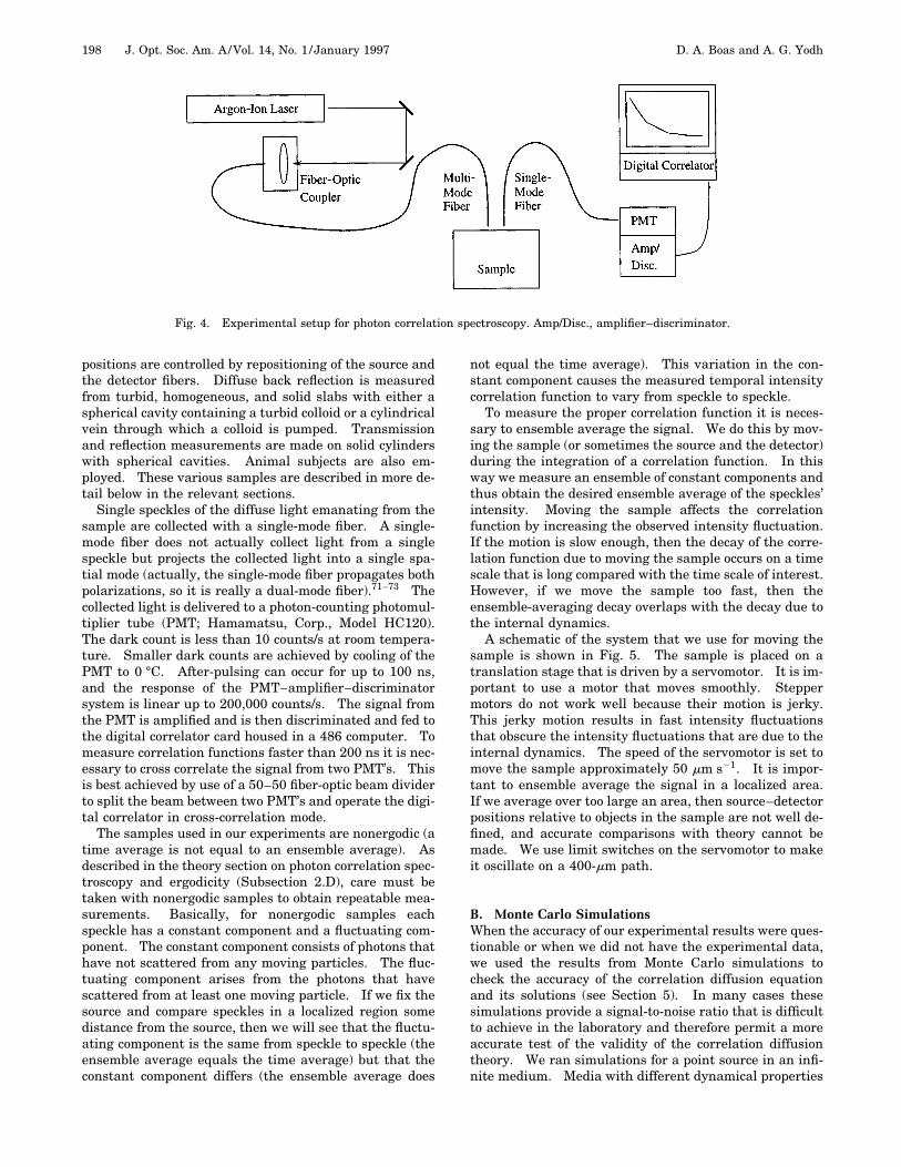
198 J. Opt. Soc. Am. A/Vol. 14, No. 1 /January 1997 D. A. Boas and A. G. Yodh
Fig. 4. Experimental setup for photon correlation spectroscopy. Amp/Disc., amplifier–discriminator.
positions are controlled by repositioning of the source andthe detector fibers. Diffuse back reflection is measuredfrom turbid, homogeneous, and solid slabs with either aspherical cavity containing a turbid colloid or a cylindricalvein through which a colloid is pumped. Transmissionand reflection measurements are made on solid cylinderswith spherical cavities. Animal subjects are also em-ployed. These various samples are described in more de-tail below in the relevant sections.Single speckles of the diffuse light emanating from the
sample are collected with a single-mode fiber. A single-mode fiber does not actually collect light from a singlespeckle but projects the collected light into a single spa-tial mode (actually, the single-mode fiber propagates bothpolarizations, so it is really a dual-mode fiber).71–73 Thecollected light is delivered to a photon-counting photomul-tiplier tube (PMT; Hamamatsu, Corp., Model HC120).The dark count is less than 10 counts/s at room tempera-ture. Smaller dark counts are achieved by cooling of thePMT to 0 °C. After-pulsing can occur for up to 100 ns,and the response of the PMT–amplifier–discriminatorsystem is linear up to 200,000 counts/s. The signal fromthe PMT is amplified and is then discriminated and fed tothe digital correlator card housed in a 486 computer. Tomeasure correlation functions faster than 200 ns it is nec-essary to cross correlate the signal from two PMT’s. Thisis best achieved by use of a 50–50 fiber-optic beam dividerto split the beam between two PMT’s and operate the digi-tal correlator in cross-correlation mode.The samples used in our experiments are nonergodic (a
time average is not equal to an ensemble average). Asdescribed in the theory section on photon correlation spec-troscopy and ergodicity (Subsection 2.D), care must betaken with nonergodic samples to obtain repeatable mea-surements. Basically, for nonergodic samples eachspeckle has a constant component and a fluctuating com-ponent. The constant component consists of photons thathave not scattered from any moving particles. The fluc-tuating component arises from the photons that havescattered from at least one moving particle. If we fix thesource and compare speckles in a localized region somedistance from the source, then we will see that the fluctu-ating component is the same from speckle to speckle (theensemble average equals the time average) but that theconstant component differs (the ensemble average does
not equal the time average). This variation in the con-stant component causes the measured temporal intensitycorrelation function to vary from speckle to speckle.To measure the proper correlation function it is neces-
sary to ensemble average the signal. We do this by mov-ing the sample (or sometimes the source and the detector)during the integration of a correlation function. In thisway we measure an ensemble of constant components andthus obtain the desired ensemble average of the speckles’intensity. Moving the sample affects the correlationfunction by increasing the observed intensity fluctuation.If the motion is slow enough, then the decay of the corre-lation function due to moving the sample occurs on a timescale that is long compared with the time scale of interest.However, if we move the sample too fast, then theensemble-averaging decay overlaps with the decay due tothe internal dynamics.A schematic of the system that we use for moving the
sample is shown in Fig. 5. The sample is placed on atranslation stage that is driven by a servomotor. It is im-portant to use a motor that moves smoothly. Steppermotors do not work well because their motion is jerky.This jerky motion results in fast intensity fluctuationsthat obscure the intensity fluctuations that are due to theinternal dynamics. The speed of the servomotor is set tomove the sample approximately 50 mm s21. It is impor-tant to ensemble average the signal in a localized area.If we average over too large an area, then source–detectorpositions relative to objects in the sample are not well de-fined, and accurate comparisons with theory cannot bemade. We use limit switches on the servomotor to makeit oscillate on a 400-mm path.
B. Monte Carlo SimulationsWhen the accuracy of our experimental results were ques-tionable or when we did not have the experimental data,we used the results from Monte Carlo simulations tocheck the accuracy of the correlation diffusion equationand its solutions (see Section 5). In many cases thesesimulations provide a signal-to-noise ratio that is difficultto achieve in the laboratory and therefore permit a moreaccurate test of the validity of the correlation diffusiontheory. We ran simulations for a point source in an infi-nite medium. Media with different dynamical properties

D. A. Boas and A. G. Yodh Vol. 14, No. 1 /January 1997 /J. Opt. Soc. Am. A 199
were considered. First, we gathered data for a systemwith spatially uniform Brownian motion. The correla-tion diffusion equation is known to be valid for this sys-tem at short correlation times. Therefore these firstsimulations worked as a test for the Monte Carlo code atearly correlation times and to demonstrate the break-down of the diffusion equation at long correlation times.Next, we ran simulations for a homogeneous solid sys-
tem containing a spherical region with scatterers under-going Brownian motion. These simulations are neces-sary to unravel systematic discrepancies betweenexperimental data and correlation diffusion theory.Finally, simulations were executed for a homogeneous
system with different volume fractions of random flow.This is a model of tissue blood flow. All the simulationswere performed assuming isotropic scattering (i.e.,g 5 0).The theoretical details pertinent to the Monte Carlo
simulation are reviewed here. A complete discussion ofderiving temporal electric-field correlation functions[g1(t)] was given in Section 2. The correlation function oflight that scatters once from a dilute suspension of non-interacting uncorrelated particles is
g1s~t! 5 exp@21/6q2^Dr2~t!&#, (19)
where q 5 kout 2 kin is the momentum transfer impartedby the scattering event (see Fig. 1) and ^Dr2(t)& is themean-square displacement of the scattering particles intime t. The magnitude of the momentum transfer isq 5 2ko sin(u/2). When photons are multiply scatteredby noninteracting uncorrelated particles, the correlationfunction is computed for a given photon path a with n un-correlated scattering events as
g1~a!~t! 5 expF2
1
6 (j51
n
qa, j2 ^Dr2~t!&G . (20)
qa, j is the momentum transfer experienced along path aat scattering site j.The general procedure for considering multiple paths is
to first relate the total dimensionless momentum transferY 5 ( j51
n qa, j2/2ko
2 5 ( j51n (1 2 cos ua, j) to the dimen-
sionless path length S 5 s/l* . Here s is the length of thephoton trajectory through the sample and l* is the photonrandom-walk step length. For large n,Y is accuratelyapproximated by the average over the scattering form fac-tor, and thus
Y ' n^1 2 cos u& 5nll*
5sl*
5 S. (21)
Fig. 5. Setup for performing the ensemble average.
Here ^ & denotes the average over the scattering form fac-tor and l is the photon scattering length that equals thephoton random-walk step length when the scattering isisotropic. Next the total correlation function is obtainedfrom the weighted average of Eq. (20) over the distribu-tion of path lengths, i.e.,
g1~t! 5 E0
`
P~S !exp@ko2^Dr2~t!&S/3#dS. (22)
Although P(S) can be determined by Monte Carlo simu-lations, it is usually found with the help of the photon-diffusion equation.This procedure has built into it two assumptions: the
relation between Y and S, and the assumption that P(S)is accurately given by the photon-diffusion equation. Forthe purposes of the Monte Carlo simulations it is desir-able to take a different approach that does not make thesetwo assumptions. As suggested by Middleton andFisher,74 and by Durian,75 the total correlation functioncan be obtained from a weighted average over the total di-mensionless momentum transfer experienced by all thephoton trajectories, i.e.,
g1~t! 5 E0
`
P~Y !expF13 Yko2^Dr2~t!&GdY. (23)
There are no assumptions in this formulation other thanthe standard noninteracting uncorrelated particles as-sumption. The drawback is that P(Y) cannot be calcu-lated analytically. However, Monte Carlo simulationsprovide a simple numerical approach to finding P(Y) fordifferent geometries. Such Monte Carlo simulations aredescribed by Middleton and Fisher,74 by Durian,75 and byKoelink et al.76
The Monte Carlo simulation follows the trajectory of aphoton, using the algorithm described below, with the ad-dition that the dimensionless momentum transfer Y is in-cremented in dynamic regions. When the photon reachesa detector, the Y associated with that photon is scored ina P(Y) histogram. After enough statistics have been ac-cumulated for P(Y) (typically 1 million to 10 million pho-tons), g1(t) can be calculated with Eq. (23).The basic idea of the Monte Carlo algorithm is to
launch N photons into the medium and to obtain a histo-gram of partial photon flux in radial and momentum-transfer channels. For our simulations N is typically 1million to 10 million, and the code takes ;2 h to run on aSun SPARC 10 Model 512 50-MHz processor or a 75-MHzPentium.There are many techniques for propagating and obtain-
ing histograms of photons within Monte Carlocalculations.77–79 To keep the code simple we mimic thephysical process as closely as possible instead of relyingon reduction techniques that purport to increase statisticswhile reducing computation (see Refs. 77–79 for discus-sions of different reduction techniques). To propagate aphoton from one interaction event to the next, the pro-gram calculates a scattering length and an absorptionlength based on the exponential distributions derivedfrom the scattering and the absorption coefficients, re-spectively. If the absorption length is shorter than thescattering length, then the photon is propagated the ab-

200 J. Opt. Soc. Am. A/Vol. 14, No. 1 /January 1997 D. A. Boas and A. G. Yodh
sorption length, scored if necessary, and terminated, anda new photon is launched from the source position. If thescattering length is shorter, then the photon is propa-gated the scattering length, scored if necessary, and thescattering angle is calculated based on the commonlyused Henyey–Greenstein phase function,78–80 and then anew scattering length and absorption length are calcu-lated. Photon propagation continues until the photon isabsorbed or escapes, or until the time exceeds a maximumset by Tgate (typically 10 ns).To exploit the spherical symmetry of the problem for in-
finite homogeneous media (the source is isotropic), spheri-cal shell detectors are centered on the point source, andthe crossing of photons across each shell is scored in theappropriate momentum-transfer and radial channels.Inward and outward crossings are scored separately sothat the Monte Carlo simulation can report the radialcomponents of the correlation flux. In this way we canobtain the correlation fluence, F(r), and the net correla-tion flux, 2D¹F(r), from the data. For our analyses weuse the correlation fluence.For problems with cylindrical symmetry, e.g., semi-
infinite media and a spherical inhomogeneity with thesource on the z axis, circular ring detectors were used.These ring detectors were contained in an xy plane andwere 2 mm wide. Photons were scored as they crossedthe rings in positive and negative z directions.
4. EXPERIMENTAL RESULTSIn this section we measure the correlation function onturbid media with spatially varying dynamics and opticalproperties. We compare these measurements with pre-dictions from correlation diffusion theory to demonstratethe accuracy of the correlation diffusion equation, and wedemonstrate that images of spatially varying dynamicscan be reconstructed. We first check the validity of themodel for systems with a spherical heterogeneity charac-terized by a different Brownian diffusion coefficient andoptical properties (Subsection 4.A). Subsection 4.B dem-onstrates an image reconstruction of a system with spa-tially varying Brownian motion. Subsection 4.C verifiesthe theory’s validity for systems with spatially varyingflow. In Subsection 4.D we show that the correlation dif-fusion equation can accurately quantify the thickness of alayered structure characterized by different dynamicalproperties. Burned tissue is essentially a layered struc-ture. This last result therefore suggests that correlationdiffusion spectroscopy can be used to quantify tissue burndepth, as is explored on a pig model in Section 6.
A. Validity of Diffusion Equation for Media withSpatially Varying Brownian MotionHere we compare experimental and theoretical results toverify the validity of the correlation diffusion equation forturbid media with spatially varying dynamical and opti-cal properties. The first experiments that we describeare performed on a turbid slab that is static and homoge-neous except for a spherical region, which is dynamic.Dynamic regions with different magnitudes of Brownianmotion and different scattering coefficients are consid-ered.
Before discussing the experiment, we briefly review thesolution to Eq. (11) for a medium that is homogeneous ex-cept for a spherical region (with radius a) characterizedby optical and dynamical properties different from thoseof the surrounding medium. The spherical region canalso be characterized by different optical properties. Theanalytic solution of the correlation diffusion equation forthis system reveals that the measured correlation func-tion outside the sphere can be interpreted as a superposi-tion of the incident correlation function plus a term thataccounts for the scattering of the correlation from thesphere, i.e.,
Fig. 6. Setup of an experiment in which a 514-nm line from anAr-ion laser (operated at 2.0 W with an etalon) is coupled into amultimode fiber-optic cable and is delivered to the surface of asolid slab of TiO2 suspended in resin. The slab has dimensionsof 15 3 15 3 8 cm. A spherical cavity with a diameter of 2.5 cmis located 1.8 cm below the center of the upper surface. The cav-ity is filled with a 0.2% suspension of 0.296-mm-diameter polysty-rene spheres at 25 °C, resulting in ms8 5 6.67 cm21, ma85 0.002 cm21, and DB 5 1.5 3 1028 cm2 s21. For the solid slab,ms8 5 4.55 cm21 and ma 5 0.002 cm21. A single-mode fiber col-lects light at a known position and delivers it to a PMT whoseoutput enters a digital autocorrelator to obtain the temporal in-tensity correlation function. The temporal intensity correlationfunction is related to the temporal field correlation function bythe Siegert relation.32,34,37 The fibers can be moved to any posi-tion on the sample surface.
Fig. 7. Experimental measurements of the temporal intensityautocorrelation function for three different source–detector pairswith a colloid present and one source–detector position withoutthe colloid. The dotted–dashed curve illustrates the correlationfunction decay that is due to ensemble averaging (i.e., no colloidis present in the spherical cavity). This decay is independent ofthe source–detector position. The dashed, dotted, and solidcurves correspond to g2(t) measured with a colloid in the cavityand the source–detector positions at 1, 2, and 3, respectively, asindicated in Fig. 8.

D. A. Boas and A. G. Yodh Vol. 14, No. 1 /January 1997 /J. Opt. Soc. Am. A 201
Fig. 8. Experimental measurements of the normalized temporal field autocorrelation function for three different source–detector pairsin comparison with theory. The geometry is illustrated in (a) and (b). With respect to an x–y coordinate system whose origin liesdirectly above the center of the spherical cavity, the source–detector axis was aligned parallel to the y axis with the source at y 5 1.0 cmand the detector at y 5 20.75 cm. Keeping the source–detector separation fixed at 1.75 cm, we made measurements at x 5 0.0, 1.0, 2.0cm, indicated by the symbols L, 1, and * , respectively. The uncertainty for these measurements is 3% and arises from uncertainty inthe position of the source and the detector. The curves were calculated with the known experimental parameters, with DB being a freeparameter (see Fig. 6). Note that larger and more rapid decays are observed when the source and the detector are nearest the dynamicsphere.
G1out~rs , rd , t! 5
S exp@iK out~t!urd 2 rsu#4pDgurd 2 rsu
1 (l50
`
Alhl~1 !
3 @Kout~t!rd#@K out~t!rd#Yl0~u, f!.
(24)
Here hl(1) are Hankel functions of the first kind and
Yl0(u, f) are spherical harmonics. The sphere is cen-
tered on the origin, and the source is placed on the z axisto exploit azimuthal symmetry. The coefficient Al is thescattering amplitude of the lth partial wave and is foundby application of the appropriate boundary conditions onthe surface of the sphere. The boundary conditions aresimilar to that for the photon-diffusion equation.81,82
Specifically, the diffuse correlation must be continuousacross the boundary, and the net flux must be normal tothe boundary, i.e., G1
out(a, t) 5 G1in(a, t) and 2Dg
outr• ¹G1
out(r, t)ur5a 5 2Dgin r • ¹G1
in(r, t)ur5a on thesurface of the sphere. G1
in(r, t) is the correlation func-tion inside the spherical object, and r is the normal vectorto the sphere. Applying these boundary conditions, wefind that
Al 52ivSK out
Dgout hl
~1 !~K outzs!Yl0* ~p, 0!
3 F Dgoutxjl8~x !jl~y ! 2 Dg
in yjl~x !jl8~y !
Dgoutxhl
~1 !8~x !jl~y ! 2 Dginyhl
~1 !~x ! jl8~y !G , (25)
where jl are the spherical Bessel functions of the firstkind, x 5 Kouta, y 5 K ina, a is the radius of the sphere,rs is the position of the source, and jl8 and hl
(1)8 are thefirst derivatives of the functions jl and h l
(1) with respectto the argument. This solution has been discussed in de-tail for diffuse photon-density waves.81,82
We demonstrate the scattering of temporal correlationby a dynamical inhomogeneity in an experiment shown inFig. 6. In this experiment the temporal intensity corre-lation function is measured in remission from a semi-infinite, highly scattering, solid slab of TiO2 suspended inresin (DB 5 0). The slab contains a spherical cavityfilled with a turbid, fluctuating suspension of 0.296-mmpolystyrene microspheres (DB 5 1.5 3 1028 cm2 s21).The measured temporal intensity correlation function,g2(t), for three different source–detector separations ispresented in Fig. 7. g2(t) is plotted for the system withno Brownian motion (i.e., no colloid is present) to illus-trate the time scale of the decay introduced by ensembleaveraging. From the raw data we can see that b ' 0.5,as expected, since we are using a single-mode fiber thatpropagates the two orthogonal polarizations. We also ob-serve the short-time decay of the correlation function,which is due to Brownian motion, and the long-time decaydue to ensemble averaging. The decay due to ensembleaveraging is significant for t . 300 ms and is not depen-dent on source–detector position or separation. We focuson the decay for t , 200 ms.

202 J. Opt. Soc. Am. A/Vol. 14, No. 1 /January 1997 D. A. Boas and A. G. Yodh
Figure 8 exhibits the decay of the normalized temporalfield correlation function, g1(t), obtained from g2(t) withthe Siegert relation [Eq. (4)], and compares these resultsto theoretical predictions based on Eq. (24). The ex-pected trend is observed. When the source and the de-tector are closer to the dynamical region there is more de-cay in the correlation function, and the rate of decay isgreater. Here the largest fraction of detected photonshas sampled the dynamical region and on average hashad more scattering events in the dynamical region. Thequantitative agreement between experiment and theoryis not good; to obtain good agreement one must reduce theBrownian diffusion coefficient in the spherical region by afactor ;4. For the theoretical results presented in Fig. 8,DB 5 3.77 3 1029 cm2 s21, which is a factor of ;4
Fig. 9. Experimental measurements of the normalized field cor-relation function for a dynamical region (a) with three differentms8 values plotted and (b) for three different DB values. Thesource and the detector were separated by 1.5 cm and were cen-tered over the position of the sphere. In (a) the symbols L, 1,and * correspond to ms8 5 3.5, 4.5, 9.0 cm21, respectively. Thecurves were calculated with the known experimental param-eters, with DB being a free parameter. In (b) the symbols, L,1, and * correspond to a 5 0.813, 0.300, 0.137 mm, respectively.
smaller than the expected DB 5 1.5 3 1028 cm2 s21.The cause of this discrepancy is discussed below.Correlation functions were measured for different re-
duced scattering coefficients and Brownian diffusion coef-ficients for the dynamical region. Figure 9(a) plots themeasured correlation functions for different ms8 comparedwith theory. Three different concentrations of 0.813-mm-diameter polystyrene microspheres were used to obtainreduced scattering coefficients of 3.5, 4.5, and 9.0 cm21for the dynamical region. The rest of the system is thesame as the previous experiment (see Fig. 6). With theBrownian diffusion coefficient as a free parameter to fitthe theory to experiment, good agreement was obtained.In all the cases the Brownian diffusion coefficient had tobe reduced by a factor of ;3. For 0.813-mm-diameterpolystyrene microspheres the expected DB value is 5.463 1029 cm2 s21. For ms8 5 3.5, 4.5, 9.0 cm21 the fitsfor DB were 2.21 3 1029, 2.14 3 1029, and 1.783 1029 cm2 s21, respectively.Correlation functions for different Brownian diffusion
coefficients are plotted in Fig. 9(b). Different DB valueswere obtained by use of monodisperse polystyrene micro-spheres with diameters of 0.137; 0.300; and 0.813 mm.The concentrations were varied to keep ms85 4.5 cm21. Once again, good agreement between ex-periment and theory was observed by use of a smallerDB value in the theory. The relative values for the fittedDB agree with those of the experimental DB . The ex-pected values of DB were 3.28 3 1028, 1.50 3 1028, and5.46 3 1029 cm2 s21, respectively, for the polystyrenemicrospheres with diameters of 0.137, 0.300, and 0.813mm. The fitted values for DB were 1.49 3 1028, 8.213 1029, and 2.713 1029 cm2 s21.We believe that the observed disagreement in the
Brownian diffusion coefficient results from mismatches inthe indices of refraction at the resin–air and resin–colloidinterfaces. In an early analysis38 the semi-infiniteboundary condition was solved incorrectly but fortu-itously resulted in better agreement. In that case38,40
the point source was not placed a distance of l* 5 1/ms8away from the collimated source along the source axis, asin the usual treatment of a collimated source,83 but ratherat the collimated source position. Furthermore, the im-age source (to satisfy the extrapolated boundary conditionfor index-mismatched media) was positioned as if the realsource had been extended into the medium. This treat-ment resulted in quantitative agreement between theoryand experiment.Discrepancies between experiment and theory also
arise because a significant fraction of the detected pho-tons scatter from the dynamical region only a few timesbefore detection, but these discrepancies are small com-pared with those that arise from mismatches in the indi-ces of refraction.39
The high sensitivity to the treatment of the semi-infinite boundary conditions and the mismatch in the in-dices of refraction renders this experimental setup inap-propriate for rigorously validating the correlationdiffusion equation for systems with spatially varying dy-namical and optical properties. In Subsection 4.B wecompare the theory with Monte Carlo results for infinitemedia with spherical inhomogeneities and obtain quanti-

D. A. Boas and A. G. Yodh Vol. 14, No. 1 /January 1997 /J. Opt. Soc. Am. A 203
tative agreement. The agreement supports the view thatcorrelation scatters from spatial variations of the particlediffusion coefficient [DB(r)], the absorption [ma(r)], andthe reduced scattering coefficient @ms8(r)#.
B. Image Reconstruction in Media with SpatiallyVarying Brownian MotionSince the perturbation of correlation by inhomogeneitiescan be viewed as a scattering process, one readily can en-vision the application of tomographic algorithms for thereconstruction of images of spatially varying dynamics.13
We have investigated this possibility. We use an inver-sion algorithm, one of several possible schemes,13,84 whichis based on a solution to the correlation diffusion equa-tion, Eq. (11), generalized to include spatially varying dy-namics, DB(r) 5 DB,o 1 dDB(r), absorption, ma(r)5 ma,o 1 dma(r), and scattering, ms8(r) 5 ms,o81 dms8(r) and Dg(r) 5 Dg,o 1 dDg(r). DB,o , ms,o8 , andma,o are the spatially uniform background characteristics.dma(r) is the spatial variation in the absorption coeffi-cient, dms8(r) is the spatial variation in the reduced scat-tering coefficient, dDg (r) is the spatial variation in thephoton-diffusion coefficient, and dDB(r) represents thespatial variation in the particle diffusion coefficient rela-tive to the background value.The steady-state correlation diffusion equation with
spatially varying optical and dynamical properties is
¹2G1~rs , r, t! 2vma,o
Dg,oG1~rs , r, t!
22vms8ko
2DB,ot
Dg,oG1~rs , r, t!
5 2v
Dg~r!Sod~rs 2 r! 1
1ms,o8
¹dms8~r!
• ¹G1~rs , r, t! 1vdma~r!
Dg,oG1~rs , r, t!
12vms8ko
2dDB~r!t
Dg,oG1~rs , r, t!
1 3ma,odms8G1~rs , r, t!. (26)
This equation can be solved with the first Born approxi-mation or the Rytov approximation.84 Within the Rytovapproximation we assume that G1(rs , rd , t)5 G1
o(rs , rd , t)exp@Fs(rs , rd , t)#. Following the pro-cedure described by Kak and Slaney,84 we obtain an inte-gral equation relating Fs(rs , rd , t) to the spatial varia-tion of the dynamical and optical properties, i.e.,
Fs~rs , rd , t! 5 21
G1o~rs , rd , t!
3 E d3r8F2vms8ko2tdDB~r8!
Dg,o
3 H~r8, rd , t!G1o~rs , r8, t!
1vdma~r8!
Dg,oH~r8, rd , t!G1
o~rs , r8, t!
1dDg~r8!
Dg,o¹G1
o~rs , r8! • ¹H~r8, rd!G .(27)
Here H(r8, rd , t) is the Green’s function for the homoge-neous correlation diffusion equation. The position of thesource (detector) is rs (rd).There are many techniques that can be employed to in-
vert Eq. (27).13,84 All the methods are based on discretiz-ing the integral equation and using measurements ofFs(rs , rd) with several different source–detector pairs tosolve the coupled set of linear equations. We use the si-multaneous iterative reconstruction technique84 to solvethe coupled equations.To demonstrate that the correlation diffusion equation
can be used as the basis for a tomographic reconstructionalgorithm, we took several measurements of the correla-tion function on a solid, highly scattering sample thatcontained a spherical, dynamical region. The systemwas a solid cylinder of TiO2 suspended in resin. The cyl-inder was homogeneous except for a 1.3-cm-diameterspherical cavity that was filled with an aqueous suspen-sion of 0.296-mm polystyrene microspheres (DB 5 1.53 1028 cm2 s21) and centered at z 5 0 (the z axis is theaxis of the cylinder). The optical properties (ms8 , ma) ofthe colloid matched that of the solid so that we imagedonly variations in the dynamical properties. Measure-ments were made every 30° at the surface of the cylinderfor z 5 0, 1, 2 cm, with source–detector angular separa-tions of 30° and 170° and correlation times of t5 15, 25, 35, 45, 55, 65, 75, 85 ms. Except wherethe measurements were made, a highly reflective coatingwas applied to the surface so that the cylindrical mediumcould be better approximated as infinite. This approxi-mation was discussed by Haskell et al.,83 and its validityallows us to obtain accurate reconstructions of the dy-namical properties.The image of DB(r) shown in Fig. 10 was reconstructed
from ;600 measurements of the scattered correlationfunction, Fs(rs , rd , t), with 400 iterations of the simulta-neous iterative reconstruction technique.84 The z 5 0slice of the image is shown in Fig. 10(a). From this im-age the center (in the x–y plane) of the dynamic regionand the magnitude of the particle diffusion coefficient aredetermined. The center of the object in the image iswithin 2 mm of the actual center of the dynamic sphere.This discrepancy scales with the uncertainty in the posi-tion of the source and the detector. The sphere diameter(;1.3 cm) and the particle diffusion coefficient (;1.83 1028 cm2 s21) obtained from the imaging procedurealso agree reasonably well with experimentally knownparameters (1.3 cm and 1.5 3 1028 cm2 s21).
C. Validity of Diffusion Equation for Media withSpatially Varying Flow PropertiesThe experiments described thus far demonstrate the dif-fusion and the scattering of correlation in turbid samplesin which the dynamics are governed by Brownian motion.The correlation diffusion equation can be modified to ac-count for other dynamical processes. In the cases of ran-dom flow and shear flow the correlation diffusion equationbecomes
~Dg¹2 2 vma 2 2vms8DBko2t 2 1/3 vms8^DV
2&ko2t2
2 1/15 vms821Geff
2ko2t2!G1~r, t! 5 2vS~r!. (28)

204 J. Opt. Soc. Am. A/Vol. 14, No. 1 /January 1997 D. A. Boas and A. G. Yodh
The fourth and the fifth terms on the left-hand side of Eq.(28) arise from random and shear flows, respectively.^DV2& is the second moment of the particle speed distribu-tion (assuming that the velocity distribution is isotropicand Gaussian),30,85 and Geff is the effective shear rate.56
Notice that the dynamical absorption for flow in Eq. (28)increases as t 2 (compared with the t increase for Brown-ian motion) because particles in flow fields travel ballisti-cally; also, DB , ^DV2&, and Geff appear separately becausethe different dynamical processes are uncorrelated. Theform of the dynamical absorption term for random flow isrelated to that for Brownian motion. Both are of theform 1
3 vms8^Dr2(t)&, where ^Dr2(t)& is the mean-square
displacement of a scattering particle. For Brownian mo-tion ^Dr2(t)& 5 6DBt, and for random flow ^Dr2(t)&5 ^DV2&t 2. The derivation of the dynamical absorptionterm for shear flow is more complex, and the reader is re-ferred to Wu et al.56 for a complete discussion.Flow in turbid media is an interesting problem that has
received some attention. In these measurements experi-menters typically determine a correlation function thatmay be a compound of many decays representing aweighted average of flow within the sample. For ex-ample, Bonner and Nossal developed an approach for
Fig. 10. (a) Image reconstructed from experimental measure-ments of the scattered correlation function. The system was a4.6-cm-diameter cylinder with l* 5 0.25 cm, ma 5 0.002 cm21,and DB 5 0 [see illustration in (b)]. A 1.3-cm-diameter spheri-cal cavity was centered at x 5 0.7 cm, y 5 0, and z 5 0 and wasfilled with a colloid with l* 5 0.25 cm, ma 5 0.002 cm21, andDB 5 1.5 3 1028 cm2 s21. A slice of the image at z 5 0 cm ispresented in (a). The values of the reconstructed particle diffu-sion coefficients are indicated by the legend in units of squarecentimeters per second.
measuring random blood flow in homogeneous tissue30;Wu et al. applied DWS to study uniform shear flow56; andBicout and co-workers applied DWS to study inhomoge-neous flow and turbulence.86–89 In all the cases, a prioriknowledge of the flow is used in the analyses. The appli-cation of correlation diffusion imaging will further clarifyinformation about heterogeneous flows in turbid media.We conducted experiments to examine the correlation
signal arising from a solid highly scattering medium witha single cylindrical vein containing a highly scattering liq-uid under Poiseuille flow. The experimental system isdepicted in Fig. 11. In this experiment the correlationfunction is measured in remission from a semi-infinite,highly scattering, solid slab of TiO2 suspended in resin(Geff 5 0). A 0.5% solution of Intralipid90 is pumpedthrough the cylindrical vein in the slab with pump speedsof 0.442 cm s21, 0.884 cm s21, and 1.77 cm s21. The ex-perimental results are shown by the symbols in Fig. 12.Measurements of the normalized temporal field corre-
lation function were compared with the exact solution ofcorrelation scattering from cylindrical inhomogeneities.The derivation of the analytic solution for a cylinder issimilar to that for a sphere. Once again, the correlationis a superposition of the incident and the scattered corre-lation, i.e., G1
out 5 G1o 1 G1
scatt . For a cylinder of infi-nite length, the solution for the scattered wave in cylin-drical coordinates is66
G1scatt~r, u, z !
5 2vS
2p2Dg(n51
` E0
`
dp cos~nu!cos~pz !
3 Kn@Ap2 2 ~Kout!2r#Kn@Ap2 2 ~Kout!2rs#
3 F DgoutxIn8~x !In~y ! 2 Dg
inyIn~x !In8~y !
DgoutxKn8~x !In~y ! 2 Dg
inyKn~x !In8~y !G ,
(29)where In and Kn are modified Bessel functions, x5 Ap2 2 (Kout)2a, y 5 Ap2 2 (K in)2a, and a is the ra-dius of the cylinder. We have simplified the solution bytaking the z axis as the axis of the cylinder and assumingthat the source is at z 5 0 and u 5 0°.The comparison between experiment (symbols) and
theory (curves) shown in Fig. 12 indicates a good agree-ment. The parameters used in the calculation, except forGeff , were the known parameters. We determined the ef-fective shear rate, Geff , by fitting the analytic solution tothe data with the constraint that Geff had to scale linearlywith the flow speed. The best fit to the data indicatesthat Geff is approximately 6.8 cm21 times the flow speed.Since the shear rate is given by the change in speed perunit length in the direction perpendicular to the flow, onemight expect that the effective shear rate would be theflow speed divided by the radius of the vein. This simplecalculation gives an effective shear rate that is a factor of2 smaller than the measured Geff . This difference is notyet understood, but it could result from the mismatches inoptical indices of refraction and sensitivity to the semi-infinite boundary condition.
D. A. Boas and A. G. Yodh Vol. 14, No. 1 /January 1997 /J. Opt. Soc. Am. A 205
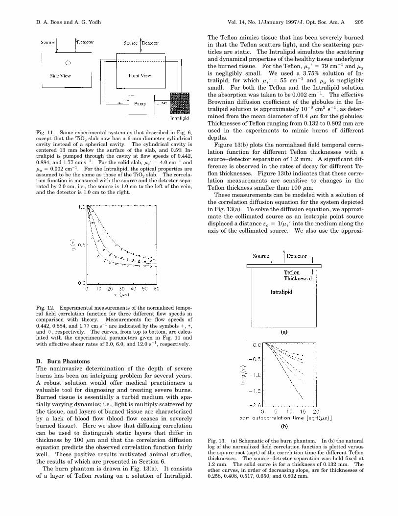
D. Burn PhantomsThe noninvasive determination of the depth of severeburns has been an intriguing problem for several years.A robust solution would offer medical practitioners avaluable tool for diagnosing and treating severe burns.Burned tissue is essentially a turbid medium with spa-tially varying dynamics; i.e., light is multiply scattered bythe tissue, and layers of burned tissue are characterizedby a lack of blood flow (blood flow ceases in severelyburned tissue). Here we show that diffusing correlationcan be used to distinguish static layers that differ inthickness by 100 mm and that the correlation diffusionequation predicts the observed correlation function fairlywell. These positive results motivated animal studies,the results of which are presented in Section 6.The burn phantom is drawn in Fig. 13(a). It consists
of a layer of Teflon resting on a solution of Intralipid.
Fig. 11. Same experimental system as that described in Fig. 6,except that the TiO2 slab now has a 6-mm-diameter cylindricalcavity instead of a spherical cavity. The cylindrical cavity iscentered 13 mm below the surface of the slab, and 0.5% In-tralipid is pumped through the cavity at flow speeds of 0.442,0.884, and 1.77 cm s21. For the solid slab, ms8 5 4.0 cm21 andma 5 0.002 cm21. For the Intralipid, the optical properties areassumed to be the same as those of the TiO2 slab. The correla-tion function is measured with the source and the detector sepa-rated by 2.0 cm, i.e., the source is 1.0 cm to the left of the vein,and the detector is 1.0 cm to the right.
Fig. 12. Experimental measurements of the normalized tempo-ral field correlation function for three different flow speeds incomparison with theory. Measurements for flow speeds of0.442, 0.884, and 1.77 cm s21 are indicated by the symbols 1, * ,and L, respectively. The curves, from top to bottom, are calcu-lated with the experimental parameters given in Fig. 11 andwith effective shear rates of 3.0, 6.0, and 12.0 s21, respectively.
The Teflon mimics tissue that has been severely burnedin that the Teflon scatters light, and the scattering par-ticles are static. The Intralipid simulates the scatteringand dynamical properties of the healthy tissue underlyingthe burned tissue. For the Teflon, ms8 5 79 cm21 and mais negligibly small. We used a 3.75% solution of In-tralipid, for which ms8 5 55 cm21 and ma is negligiblysmall. For both the Teflon and the Intralipid solutionthe absorption was taken to be 0.002 cm21. The effectiveBrownian diffusion coefficient of the globules in the In-tralipid solution is approximately 1028 cm2 s21, as deter-mined from the mean diameter of 0.4 mm for the globules.Thicknesses of Teflon ranging from 0.132 to 0.802 mm areused in the experiments to mimic burns of differentdepths.Figure 13(b) plots the normalized field temporal corre-
lation function for different Teflon thicknesses with asource–detector separation of 1.2 mm. A significant dif-ference is observed in the rates of decay for different Te-flon thicknesses. Figure 13(b) indicates that these corre-lation measurements are sensitive to changes in theTeflon thickness smaller than 100 mm.These measurements can be modeled with a solution of
the correlation diffusion equation for the system depictedin Fig. 13(a). To solve the diffusion equation, we approxi-mate the collimated source as an isotropic point sourcedisplaced a distance zo 5 1/ms8 into the medium along theaxis of the collimated source. We also use the approxi-
Fig. 13. (a) Schematic of the burn phantom. In (b) the naturallog of the normalized field correlation function is plotted versusthe square root (sqrt) of the correlation time for different Teflonthicknesses. The source–detector separation was held fixed at1.2 mm. The solid curve is for a thickness of 0.132 mm. Theother curves, in order of decreasing slope, are for thicknesses of0.258, 0.408, 0.517, 0.650, and 0.802 mm.

206 J. Opt. Soc. Am. A/Vol. 14, No. 1 /January 1997 D. A. Boas and A. G. Yodh
mate extrapolated-zero boundary condition instead of theexact zero-flux boundary condition (partial flux in thecase of an index mismatch). For the extrapolated-zeroboundary condition the field correlation is taken to bezero at z 5 zb 5 22/(3ms8), where the physical boundaryis at z 5 0. The diffusion equation must be solved fortwo cases: (1) when the point source is in the staticlayer, and (2) when the point source is displaced into thedynamic region [see Fig. 13(a)]. In the first case, G1(r, t)measured on the surface of the static layer a distance rfrom the source is given by
G1~r, t!
5
exp@2k1~t!Ar2 1 zo2#
4pAr2 1 zo2
2exp@2k1~t!Ar2 1 ~zo 1 2zb!2#
4pAr2 1 ~zo 1 2zb!2
1 E0
`
ldlA~l!J0~lr!
sin@Ak12~t! 2 l2~z 1 zb!#
Ak12~t! 2 l2
.
(30)
Here k12(t) 5 v (1)ma
(1)/Dg(1) is the correlation wave num-
ber in the static layer, J0(x) is a cylindrical Bessel func-tion, and A(l) is a constant that depends on the thicknessof the static layer and on the properties of the dynamicalmedium. This constant is
the small static layer. In this regime comparison with asolution of the correlation transport equation61,62 wouldbe more appropriate.
5. MONTE CARLO SIMULATIONS
This section presents the results of various Monte Carlosimulations of correlation diffusion. We used the resultsfrom Monte Carlo simulations to check the accuracy of thecorrelation diffusion equation when the accuracy of ourexperimental results was questionable or when we did nothave the experimental data. These simulations allow usto obtain data for systems with no variation in the indexof refraction. In many cases these simulations provide asignal-to-noise ratio that is difficult to achieve in the labo-ratory and therefore permit a more accurate test of thevalidity of the correlation diffusion theory.We first present simulation results for an infinite, ho-
mogeneous system compared with correlation diffusiontheory. This comparison illustrates the behavior of thecorrelation function as different parameters are varied.Good agreement with diffusion theory is observed. Wethen present results for a system that is infinite, static,and homogeneous, except for a spherical dynamic region.This system avoids the shortcomings of the experimentalsystem used in Section 4. Results are compiled for awide range of parameters and are compared with correla-tion diffusion theory. The agreement is good, indicatingthe robustness of the theory. We then present simula-tions for a two-component system with spatially uniformrandom flow in a spatially uniform static medium. This
A~l! 5 2$exp@iX~l!~d 2 zo!# 2 exp@iX~l!~d 1 2zb 1 zo!#%
3Dg
~2 !Y~l! 2 Dg~1 !X~l!
Dg~1 !X~l!cos@X~l!~d 1 zb!# 2 iDg
~2 !Y~l!sin@X~l!~d 1 zb!#, (31)
with X(l) 5 Ak12(t) 2 l2 and Y(l) 5 Ak22(t) 2 l2,where k2(t) 5 @v (2)ma
(2) 1 2vms8(2)DBko
2t#/Dg(2) is the cor-
relation wave number in the dynamical medium.The solution for the second case is
G1~r, t! 5 E0
`
ldlJ0~lr!22iDg
~2 ! exp@iY~l!~zo 2 d !#
Dg~1 !X~l!cos@X~l!~d 1 zb!# 2 iDg
~2 !Y sin@X~l!~d 1 zb!#sin@X~l!zb#. (32)
Comparisons between experiment and diffusion theoryare made in Fig. 14. The parameters used in the calcu-lation are given in the text’s discussion of Fig. 13(a). Theagreement between experiment and theory, although notperfect, is pretty good and certainly captures the trend asa function of source–detector separation and static-layerthickness. It is interesting that the agreement is betterat larger thicknesses, where the diffusion theory is ex-pected to be more valid in the static layer. The largerdisagreement at smaller thicknesses is most likely a re-sult of the breakdown of the diffusion approximation in
system models a capillary network in tissue. The com-parison with correlation diffusion theory demonstratesthat the homogeneous solution can be used as long as thedynamical term is weighted by
ms8~random flow component!ms8~random flow component! 1 ms8~static component!
.
(33)
The Monte Carlo simulations for obtaining electric-fieldtemporal autocorrelation functions are described in Sub-section 3.B. Briefly, the approach is to histogram the ac-cumulated momentum transfer of photons scattered frommoving particles as they propagate through a system withspatially varying dynamics. That is, scattering events ina static medium do not contribute to the accumulated mo-

D. A. Boas and A. G. Yodh Vol. 14, No. 1 /January 1997 /J. Opt. Soc. Am. A 207
mentum transfer, whereas scattering events in a dynamicmedium do contribute. The contribution is proportionalto the magnitude of the dynamics. In the simulation themomentum transfer is accumulated as a dimensionlessvariable that scales with ko
2. The histogram, when nor-malized, is the momentum-transfer probability distribu-tion P(Y). The correlation function can then be calcu-lated with74,75
g1~t! 5 E0
`
dYP~Y !expF213Yko
2^Dr2~t!&G . (34)
P(Y) is determined from the Monte Carlo simulation, ko2
is the wave number of light in the medium, and ^Dr2(t)& isdetermined by the dynamics of the system.
A. Homogeneous Media with Brownian MotionFigure 15 plots the Monte Carlo results and the predic-tions of theory [Eq. (13)] for different source–detectorseparations r in an infinite medium. The optical and thedynamical properties are held constant at ms8 5 10.0cm21, ma 5 0.05 cm21, and DB 5 1 3 1028 cm2 s21. Thedecay rate of g1(t) increases linearly with r, as expected.Next, we can see the plateau at early t and that the tran-sition time is independent of r. Finally, g1(t) calculatedwith correlation diffusion theory for the different source–detector separations is given by the curves. In all thecases good agreement is observed when ko
2^Dr2(t)& ! 1.As expected, the agreement is not good at longer correla-tion times because of the breakdown of the approximationthat ko
2^Dr2(t)& ! 1. The results indicate that the ap-proximation is not valid when ko
2^Dr2(t)& > 0.1, that is,when t > 225 ms.
Fig. 14. Comparisons between the experimental data and thosepredicted by theory for different thicknesses and separations.Each graph shows the results for a particular thickness of Teflon.The solid curves are the experimental data, and the dottedcurves are theoretical data. Results for separations of 0.4, 0.8,1.2, and 1.8 mm are given.
The behavior of the deviation is understood. At longercorrelation times the decay results from shorter photonpath lengths, since the longer path lengths have a fasterdecay rate and no longer provide a significant contribu-tion. For the shorter path lengths the photon-diffusionapproximation is not valid, inasmuch as the photons arenot diffusing. Furthermore, the q average is not appro-priate, since there have been only a few scattering events,and, for the photon to reach the detector, the scatteringangles must be smaller than average. The smaller-than-average scattering angles result in the observed slowerdecay rate of the Monte Carlo simulations relative to dif-fusion theory.
B. Media with Spatially Varying Brownian MotionHere we present Monte Carlo results to check the validityof the correlation diffusion equation for systems with spa-tially varying dynamical and optical properties. The sys-tem is infinite, static, and homogeneous, except for aspherical region that is dynamic and may have differentoptical properties than the background. The homoge-neous properties are ms8 5 10.0 cm21 and DB 5 0. Forthe sphere, ms8 5 10.0 cm21 and DB 5 1 3 1028
cm2 s21. The absorption coefficients are varied. Resultsare presented for the source–detector positions indicatedin Fig. 16(a).Comparison of Monte Carlo results and correlation dif-
fusion theory for a system with spatially varying dynami-cal properties but uniform optical properties is presentedin Figs. 16(b)–16(d). Three different absorption coeffi-cients are considered. In Figs. 16(b), 16(c), and 16(d) theabsorption coefficients are ma 5 0.02 cm21, ma
Fig. 15. Comparison between Monte Carlo simulations for cor-relation diffusion in a homogeneous medium and predictions oftheory for different source–detector separations. Monte Carloresults are given by the symbols. The solid curves are calcu-lated from diffusion theory. ms8 5 10.0 cm21, ma8 5 0.05 cm21,and DB 5 1.0 3 1028 cm2 s21.

208 J. Opt. Soc. Am. A/Vol. 14, No. 1 /January 1997 D. A. Boas and A. G. Yodh
Fig. 16. Comparison between Monte Carlo results for the g1(t) (symbols) and correlation diffusion theory (solid curves) for the systemdepicted in (a). An isotropic point source is positioned 1.0 cm from the center of a spherical inhomogeneity. The sphere has a diameterof 1 cm. Detectors are positioned 1.0 cm away along the z axis and are displaced off the z axis at r 5 1, 2, 3 cm. The optical propertiesare spatially uniform. In (b), (c), and (d) the absorption coefficient ma 5 0.02, 0.05, 0.10 cm21, respectively. The r position of the de-tector is indicated in the legend.
5 0.05 cm21, and ma 5 0.10 cm21, respectively. Foreach absorption coefficient, results are presented for thethree detector positions. The Monte Carlo results aregiven by the symbols, and the curves indicate the predic-tion of correlation diffusion theory. The agreement isfairly good. For other Brownian diffusion coefficients, tscales inversely with DB , as expected and as observed ex-perimentally (see Fig. 9).The small discrepancies are most likely due to the fact
that a significant fraction of the fluctuating photons havescattered from the dynamical region only a few times be-fore detection.39 By ‘‘fluctuating photons’’ we mean thosephotons that have sampled the dynamic region as op-posed to the static photons that have not seen the dy-namic region.
C. Media with Random FlowTissue blood flow is a good example of an optically turbidmedium with random flow. Capillary networks are gen-erally randomly oriented on length scales set by the pho-ton random-walk step length. When the capillary flow isoriented, as it is in muscle, the photon generally scatters101 times between interactions with blood such that thephoton’s direction is randomized between blood interac-tions. Thus the flow is effectively random. Tissue bloodflow can be modeled as a two-component system, the
Fig. 17. Comparison of Monte Carlo simulations and correlationdiffusion theory for random flow in a static tissuelike matrix.The probability of scattering from a flow particle (blood) is 0.1.

D. A. Boas and A. G. Yodh Vol. 14, No. 1 /January 1997 /J. Opt. Soc. Am. A 209
static tissue matrix and the randomly flowing blood.30,91
Monte Carlo results for this system are compared withcorrelation diffusion theory predictions.Because the system is composed of two uniformly dis-
tributed components, it is necessary to modify the corre-lation diffusion equation to account for the volume frac-tion of blood. One does this by simply weighting thedynamical absorption term by the probability of scatter-ing from a red blood cell, i.e.,
~Dg¹2 2 vma 2 1/3 Pbloodvms8ko2^DV2&t2!G1~r, t!
5 2vS~r!. (35)
Pblood is the probability of scattering from a red blood celland is given by
Pblood 5ms8~blood!
ms8~blood! 1 ms8~static component!. (36)
The other optical parameters in Eq. (35) account for thecombined contribution from the tissue matrix and theblood.A comparison of the Monte Carlo results and correla-
tion diffusion theory is presented in Fig. 17 for Pblood5 0.1 The optical properties are ms8 5 10.0 cm21 andma 5 0.05 cm21. The mean-square speed of the red bloodcells is ^DV2& 5 1.0 mm2 s22. The agreement is quitegood when ko
2^DV2&t 2 ! 1, indicating that the diffusiontheory can be used to quantify blood flow in particularand random flow in turbid media in general. The smalldiscrepancy observed for times greater than 25 ms arisesfrom the assumption that ko
2^DV2&t2 ! 1 [note that(ko
2^DV2&)21/2 5 61 ms]. Comparisons were made forother Pblood values, and in all the cases good agreementwas observed.
6. DIAGNOSING TISSUE BURN DEPTHAfter verifying with measurements on phantoms thatphoton correlation techniques are sensitive to differencesin thickness of 100 mm and that the correlation diffusionequation [Eq. (11)] can be used to model the correlationfunction (see Subsection 4.D), we applied diffuse correla-tion spectroscopy in a clinical environment. The clinicalwork was done with Norm Nishioka and KevinSchomacker at the Wellman Institute in Boston, Massa-chusetts. We used their pig burn model and protocol forthe clinical trials.92
To probe burn depth, we used the experimental systemdepicted in Fig. 18. The laser light is coupled into a mul-timode optical fiber (core diameter, 200 mm). This fiberdelivers the light to the pig. Several single-mode fibersare positioned with the source fiber to collect light at dis-tances ranging from 0.2 to 2.4 mm from the source. Thelight collected with the single-mode fibers is then deliv-ered to a photon-counting PMT and is analyzed with adigital temporal autocorrelator. In the experiments pre-sented here, approximately 4 mW of light is incident uponthe sample, and the signal is integrated for 1 min. Thepig was anesthetized and was stabilized on an operatingtable in an operating suite at the Wellman Institute.Burns were administered with 2-in.-square metal blocksbrought to 100 °C by means of boiling water. Burn thick-
ness was controlled by application of the metal block tothe skin for a duration of 1–20 s. For our study, five dif-ferent burns were examined. The duration and thedepth of each burn is provided in Table 1. The measure-ments were made 48 h after administration of the burn.Prior to burning the tissue, measurements were made
at various positions on the skin to determine a baseline.Also, baselines were periodically measured on healthy tis-sue between measurements of the burned tissue. For thehealthy tissue, we observed a single exponential decay inthe correlation function and saw that the decay rate in-creased linearly with the source–detector separation.Figure 19 plots the temporal field correlation functions
obtained from the 48-h-old burns for a source–detectorseparation of 800 mm. As expected, the decay rate of thecorrelation function decreases as the burn thickness in-creases. These data indicate that the 5-, 7-, 12-, and20-s, burns are easily distinguished. To summarize thedata for all the source–detector separations, we deter-mined the decay rate of the correlation function for0 , t , 100 ms by fitting a line to the data, and we plotthe decay rate as a function of source–detector separationfor different burns. These results are given in Fig. 20
Fig. 18. Experimental setup for the pig experiments. Theshaded areas on the pig indicate burns of various depths.
Table 1. Burn Depths Were Assessed from Biop-sied Tissue by Use of a Lactate Dehydrogenase
Staina
Duration of Burn (s) Burn Depth (mm)
3 60–100 (epidermal)5 400–5007 500–60012 1500–200020 2100–2200
aLactate dehydrogenase is a vital stain; therefore it will not stain cellsthat are deadened by the burn.

210 J. Opt. Soc. Am. A/Vol. 14, No. 1 /January 1997 D. A. Boas and A. G. Yodh
and indicate that it is possible to distinguish burns thatvary in thickness by only 100 mm. The behavior of thedecay rate is expected. For shallow burns, the decay rateincreases linearly with the source–detector separation, asobserved for healthy tissue and as expected for a homoge-neous system; i.e., the shallow burn does not perturb thecorrelation function. However, for deeper burns, the de-cay rate decreases and no longer increases linearly withthe source–detector separation.Our results from this clinical study are encouraging in
that they verify that correlation measurements can beused to distinguish burns with thicknesses that vary by100 mm. More research is needed to quantify the burnthickness from the raw data. The quantification will re-quire knowledge of the optical and the dynamical proper-ties of the burn. It should be possible to determine these
Fig. 19. Plot of temporal field correlation functions obtainedfrom the 48-h-old burns for a source–detector separation of 800mm. The correlation functions for the 3-s (solid curve), 5-s (dot-ted curve), 7-s (dashed curve), 12-s (dotted–dashed curve), andthe 20-s (top curve) burns are presented.
Fig. 20. Graph of decay rate of the correlation function versussource–detector separation for different burns. The burndepths are indicated in the legend.
quantities from the correlation measurements and fromdiffuse reflectance measurements in the time domainand/or the frequency domain. One may simplify thisquantification by comparing correlation functions be-tween burned and healthy tissue. A ratio of such mea-surements may be insensitive to blood flow, thus reducingthe number of unknowns in the determination of the burndepth. Finally, the behavior of the burns during the firstfew hours must be studied carefully to determine whethercorrelation techniques can be used to diagnose the sever-ity of fresh burns. To be a suitable diagnostic tool, ourtechnique must be able to characterize burns during thefirst day, preferably within the first 6 h. This research isin progress.
7. SUMMARYWe have shown that the transport of temporal electric-field correlation through turbid media can be modeledwith a diffusion equation and is thus completely analo-gous to photon diffusion. The properties of diffusing cor-relation are thus expected to be similar to the propertiesof photon diffusion. We demonstrated this experimen-tally by showing that the migration of correlation in a tur-bid medium with spatially varying dynamical and opticalproperties can be viewed as a macroscopic scattering ofcorrelation waves. This concept was shown in the con-text of both forward and inverse problems. The inverseproblem, otherwise known as image reconstruction meth-ods, offers exciting possibilities for studying dynamicalvariations in heterogeneous turbid media. In biomedicaloptics, for example, this approach offers a simple frame-work for analyzing the complex signals obtained fromfluid flow in the body.
APPENDIX A: DIFFUSIONAPPROXIMATION TO THE CORRELATIONTRANSPORT EQUATIONThe PN approximation as described for the photon trans-port equation93–96 can be applied to the correlation trans-port equation with only a few modifications. The corre-lation transport equation is
¹ • G1T~r, V, t!V 1 m tG1
T~r, V, t!
5 msE G1T~r, V8, t!g1
s~V, V8, t!f~V, V8!dV8
1 S~r, V!. (A1)
Here G1T(r, V, t) is the unnormalized temporal field cor-
relation function, which is a function of position r, direc-tion V, and correlation time t. The scattering and theabsorption coefficients are ms and ma , respectively, andm t 5 ms 1 ma is the transport coefficient. Furthermore,g1
s(V, V8, t) is the normalized temporal field correlationfunction for single scattering; f(V, V8) is the normalizeddifferential cross section; and S(r, V) is the source distri-bution. The scattering coefficient is the reciprocal of thescattering length, ms 5 1/l, and the absorption coefficientis the reciprocal of the absorption length, ma 5 1/la . Thetime dependence (not to be confused with correlation

D. A. Boas and A. G. Yodh Vol. 14, No. 1 /January 1997 /J. Opt. Soc. Am. A 211
time) has been left out of the equation since we are con-sidering only measurements with cw sources. We can in-clude the time dependence by adding a time derivative ofG1
T(r, V, t) $i.e., v21@]/(]t)#G1T(r, V, t)% to the left-
hand side of Eq. (A1).In analogy to photon transport, the correlation fluence
is
G1~r, t ! 5 E dVG1T~r, V, t!, (A2)
whereas the correlation flux is given by
Jg~r, t ! 5 E dVG1T~r, V, t!V. (A3)
The main difference between the correlation transportequation and the photon transport equation is the ap-pearance of g1
s(V, V8, t) in the integral. The appear-ance of this angular dependent quantity will result in in-tegrals of three spherical harmonics, which are handledin a fashion similar to the handling of V • ¹f l,m(r, t) inthe photon transport equation.93–96
Within the PN approximation, G1T(r, V, t) and the
source distribution are expanded as
G1T~r, V, t! 5 (
l50
N
(m52l
l
G l,m~r, t!Yl,m~V!, (A4)
S~r, V! 5 (l50
N
(m52l
l
ql,m~r!Yl,m~V!. (A5)
For the phase function, we make the reasonable as-sumption that the amplitude is dependent only on thechange in direction of the photon, and thus
f~V • V8! 5 (l50
`2l 1 14p
gl Pl~V • V8!
5 (l50
`
(m52l
l
glYl,m* ~V8!Yl,m~V!, (A6)
where Pl is a Legendre polynomial and the second line isobtained with the angular addition rule.97 The phasefunction is normalized, and therefore g0 5 1.The single-scattering temporal field correlation func-
tion is
g1s~V, V8, t! 5 exp@21/6q2^Dr2~t!&#
5 exp@21/3ko2^Dr2~t!&~1 2 V • V8!#,
(A7)
where ^Dr2(t)& is the mean-square displacement of thescattering particles and q 5 2ko sin(u/2) is the momen-tum transfer for the scattered photon, where u is theangle between V and V8. For particles undergoingBrownian motion, ^Dr2(t)& 5 6DBt, where DB is theBrownian diffusion coefficient. When t ! (2DB ko
2)21,then Eq. (A7) is Taylor expanded to
g1s~V, V8, t! 5 1 2 2DB ko
2t 1 2DBko2t~V • V8!
5 1 2 2DB ko2t 1 2DB ko
2t4p
3
3 (m521
1
Y1,m* ~V8!Y1,m~V!. (A8)
The second line is obtained with the angular additionrule.97 Note that (2DBko
2)21 ' 1023 s when DB 5 13 1028 cm2 s21 and the wavelength of light is 514 nm.Substituting these expansions into the correlation
transport equation, Eq. (A1), we obtain
(l50
N
(m52l
l H ~V • ¹ 1 m t!G l, m~r, t!Yl, m~V!
2 ql,mYl,m~V! 2 msE dV8G l, m~r, t!Yl, m~V8!
3 (l850
N
(m852l
l
gl8Yl8, m8* ~V8!Yl8, m8~V!F1 2 2DBko2t
1 2DBko2t
4p
3 (m9521
1
Yl,m9* ~V8!Y1,m9~V!G J 5 0.
(A9)The integral over V8 can be calculated for the first twoterms between the brackets on the third and fourth linesby use of the spherical harmonic orthogonality relation.Integrating gives
(l50
N
(m52l
l
@V • ¹ 1 m t~l ! 1 glkc#G l,m~r, t!Yl,m~V!
2 ql, mYl, m~V! 2 kcE dV8G l, m~r, t!Yl, m~V8!
3 (l850
N
(m852l
l
gl8Yl8, m8* ~V8!Yl8,m8~V!
3 F4p
3 (m9521
1
Y1,m9* ~V8!Y1,m9~V!G 5 0. (A10)
New notation is introduced to simplify Eq. (A10): m t(l)
5 ms(1 2 gl) 1 ma is the reduced transport coefficient[note that m t
(0) 5 ma], and kc 5 2msDBko2t is a dynamic
absorption coefficient.Y1,m9* (V8)Yl8, m8* (V8) and Y1,m9(V)Yl8, m8(V) can be
rewritten in terms of single spherical harmonics, given(see Arfken,98 Section 12.9) as
Yl,m~V!Y1,21~V! 5 A 38p
Bl11m21Yl11,m21~V!
2 A 38p
Bl2mYl21,m21~V!, (A11)
Yl,m~V!Y1,0~V! 5 A 34p
Al11mYl11,m~V!
1 A 34p
AlmYl21,m~V!, (A12)

212 J. Opt. Soc. Am. A/Vol. 14, No. 1 /January 1997 D. A. Boas and A. G. Yodh
Yl,m~V!Y1,1~V! 5 A 38p
Bl112m21Yl11,m11~V!
2 A 38p
BlmYl21,m11~V!. (A13)
The product of spherical harmonics in the integral ofEq. (A10) can be rewritten as
4p
3 (l8m8
gl8Yl8m8* ~V8!Yl8
m8~V! (m9521
1
Y1m9* ~V8!Y1
m9~V!
54p
3 (l8m8
gl8H 38p
@Bl811m821Yl811
m821* ~V8!
2 Bl82m8Yl821
m821* ~V8!#@Bl811m821Yl811
m821~V!
2 Bl82m8Yl821
m821~V!#
134p
@Al811m8Yl811
m8* ~V8!
1 Al8m8Yl821
m8* ~V8!#@Al811m8Yl811
m8~V!
1 Al8m8Yl821
m8~V!# 238p
3 @Bl8112m821Yl811
m811* ~V8!
2 Bl8m8Yl821
m811* ~V8!#@Bl8112m821Yl811
m811~V!
2 Bl8m8Yl821
m811~V!#J . (A14)
Performing the final integral over V8, we obtain
(l50
N
(m52l
l
@V • ¹ 1 m t~l ! 1 glkc#G l,m~r, t!Yl,m~V!
2 ql,mYl,m~V! 2 kcG l,m4p
3
3 H 38p
gl21Blm@Bl
mYlm~V! 2 Bl21
2m21Yl22m~V!#
238p
gl11Bl112m21@Bl12
mYl12m~V!
2 Bl112m21Yl
m~V!# 134p
gl21Alm@Al
mYlm~V!
1 Al21mYl22
m~V!# 134p
gl11Al11m@Al12
mYl12m~V!
1 Al11mYl
m~V!# 238p
gl21Bl2m@2Bl
2mYlm~V!
1 Bl21m21Yl22
m~V!# 138p
gl11Bl11m21
3 @2Bl122mYl12
m~V! 1 Bl11m21Yl
m~V!#J 5 0.
(A15)
Next we multiply Eq. (A15) by Ya,b* (V) and integrateover V. Using the orthogonality relations for the spheri-cal harmonics, we arrive at
m t~a!Ga,b 1 gakcGa,b 2 kcF12 ~ga21Ba
bBabGa,b
2 ga11Ba12bBa11
2b21Ga12,b!
212
~ga 2 1Ba212b21Ba
bGa22,b
2 ga11Ba112b21Ba11
2b21Ga,b! 1 ~ga21AabAa
bGa,b
1 ga11Aa12bAa11
bGa12,b! 1 ~ga21Aa21bAa
bGa22,b
1 ga11Aa11bAa11
bGa,b! 212
~2ga21BBa2bBa
2b
3 Ga,b 1 ga11Ba122bBa11
b21Ga12,b!
112
~2ga21Ba21b21Ba
2bGa22,b
1 ga11Ba11b21Ba11
b21Ga,b!G 112Ba11
b21
3 S ]
]x2 i
]
]y DGa11,b21 212Ba
2bS ]
]x2 i
]
]y D3 Ga 2 1,b21 2
12Ba11
2b21S ]
]x1 i
]
]y D3 Ga11,b11 1
12Ba
bS ]
]x1 i
]
]y DGa21,b11
1 Aa11b
]
]zGa11,b 1 Aa
b]
]zGa21,b 5 qa,b . (A16)
This is a coupled set of linear differential equations forGa,b .To obtain the correlation diffusion equation, we neglect
all the Ga,b and ga values for a . 1. The a 5 0 equationis
maG0,0 1 kc~1 2 g1!G0,0 112A2
3 S ]
]x2 i
]
]y DG1,21
212A2
3 S ]
]x1 i
]
]y DG1,1 1 A13
]
]zG1,0 5 q0,0 ,
(A17)
and the a 5 1 equations are
m t~1 !G1,21 1 ~g1 2 1/3!kcG1,21 1
12A2
3 S ]
]x1 i
]
]y DG0,0
5 q1,21 , (A18)
m t~1 !G1,0 1 ~g1 2 1/3!kcG1,0 1 A1
3]
]zG0,0 5 q1,0 , (A19)
m t~1 !G1,1 1 ~g1 2 1/3!kcG1,1 2
12A2
3 S ]
]x2 i
]
]y DG0,0
5 q1,1 . (A20)

D. A. Boas and A. G. Yodh Vol. 14, No. 1 /January 1997 /J. Opt. Soc. Am. A 213
Using the definition for the correlation fluence G1(r, t)[Eq. (A2)] and the correlation flux Jg(r, t) [Eq. (A3)], wecan rewrite the a 5 0 and a 5 1 equations as
maG1~r, t! 1 1/3 ms8ko2^Dr2~t!&G1~r, t! 1 ¹ • Jg~r, t!
5 S0~r!, (A21)
m t~1 !Jg~r, t! 1 1/3 ms~g1 2 1/3!ko2^Dr2~t!&Jg~r, t!
1 1/3¹G1~r, t! 5 S1~r!. (A22)
Recall that we have assumed that correlation G1T(r, V, t)
is nearly isotropic and that the scattering particles havemoved a distance that is much smaller than a wavelengthof light. The first assumption is satisfied when ma ! msand when the scattering is not too anisotropic. The sec-ond assumption is satisfied when ko
2^Dr2(t)& ! 1. Tokeep our equations consistent with these approximationsit is necessary to drop terms from Eq. (A22); in particular,
ms8Jg~r, t! 1 1/3¹G1~r, t! 5 S1~r!. (A23)
Decoupling Eqs. (A21) and (A23) for G1(r, t), we arrive atthe correlation diffusion equation
F2¹ • S 1v Dg¹ D 1 ma 113
ms8ko2^Dr2~t!&GG1~r, t!
5 S0~r! 2 ¹ • F3v Dg S1~r!G , (A24)
where Dg 5 v/(3ms8) is the photon-diffusion coefficient.
ACKNOWLEDGMENTSThe authors thank Britton Chance for his support anddiscussions. The authors also thank Norm Nishioka andKevin Schomacker for their assistance with the animalexperiments, which were supported by the U.S. Depart-ment of the Army (grant DAMD17-94-C-4009). Theviews, opinions, and/or findings contained in this paperare those of the authors and should not be construed asan official position, policy, or decision of the U.S. Depart-ment of the Army unless so designated by other docu-ments. The authors are indebted to Maureen O’Leary forassistance with the image reconstructions and for insight-ful comments, and to Larry Campbell, Igor Meglinsky,and Laura Zemany for their technical assistance. A. G.Yodh acknowledges partial support from the National Sci-ence Foundation through the Presidential Young Investi-gator program and grant DMR93-06814 and partial sup-port from the Alfred P. Sloan Foundation.
*Present address, Electro-Optic Technology Center,Tufts University, Medford, Massachusetts 02155.
REFERENCES1. A. Yodh and B. Chance, ‘‘Spectroscopy and imaging with
diffusing light,’’ Phys. Today 48, 34–40 (1995).2. B. Chance, ed., Photon Migration in Tissues (Plenum, New
York, 1989).3. B. J. Tromberg, L. O. Svaasand, T. Tsay, and R. C. Haskell,
‘‘Properties of photon density waves in multiple-scatteringmedia,’’ Appl. Opt. 32, 607–616 (1993).
4. M. S. Patterson, B. Chance, and B. C. Wilson, ‘‘Time re-solved reflectance and transmittance for the non-invasivemeasurement of tissue optical properties,’’ Appl. Opt. 28,2331–2336 (1989).
5. G. A. Millikan, ‘‘Experiments on muscle haemoglobin in vi-vo: the instantaneous measurement of muscle metabo-lism,’’ Proc. R. Soc. London, Sect. B 129, 218–241 (1937).
6. G. A. Millikan, ‘‘The oximeter, an instrument for measuringcontinuously the oxygen saturation of arterial blood inman,’’ Rev. Sci. Instrum. 13, 434–444 (1942).
7. F. F. Jobsis, ‘‘Noninvasive, infrared monitoring of cerebraland myocardial oxygen sufficiency and circulatory param-eters,’’ Science 198, 1264–1267 (1977).
8. J. M. Schmitt, ‘‘Simple photon diffusion analysis of the ef-fects of multiple scattering on pulse oximetry,’’ IEEE Trans.Biomed. Eng. 38, 1194–1203 (1991).
9. M. R. Neuman, ‘‘Pulse oximetry: physical principles tech-nical realization and present limitations,’’ Adv. Exp. Med.Biol. 220, 135–144 (1987).
10. J. W. Severinghaus, ‘‘History and recent developments inpulse oximetry,’’ Scand. J. Clin. Lab. Invest. 53, 105–111(1993).
11. W. F. Cheong, S. A. Prahl, and A. J. Welch, ‘‘A review of theoptical properties of biological tissues,’’ IEEE J. QuantumElectron. 26, 2166–2185 (1990).
12. B. C. Wilson, E. M. Sevick, M. S. Patterson, and B. Chance,‘‘Time-dependent optical spectroscopy and imaging for bio-medical applications,’’ Proc. IEEE 80, 918–930 (1992).
13. See related studies by S. R. Arridge et al., J. P. Kaltenbachet al., and R. L. Barbour et al., in Medical Optical Tomog-raphy: Functional Imaging and Monitoring, G. Muller, B.Chance, R. Alfano, S. Arridge, J. Beuthan, E. Gratton, M.Kaschke, B. Masters, S. Svanberg, and P. van der Zee, eds.,Institute Series of SPIE Optical Engineering (Society ofPhoto-Optical Instrumentation Engineers, Bellingham,Wash., 1993), pp. 31–143.
14. S. R. Arridge, P. van der Zee, M. Cope, and D. T. Delpy, ‘‘Re-construction methods for infra-red absorption imaging,’’ inTime-Resolved Spectroscopy and Imaging of Tissues, B.Chance, ed., Proc. SPIE 1431, 204–215 (1991).
15. S. P. Gopinath, C. S. Robertson, R. G. Grossman, and B.Chance, ‘‘Near-infrared spectroscopic localization of intrac-ranial hematomas,’’ J. Neurosurg. 79, 43–47 (1993).
16. A. P. Shepherd and P. A. Oberg, eds., Laser-Doppler BloodFlowmetry (Kluwer Academic, Boston, Mass., 1990).
17. L. E. Drain, The Laser Doppler Technique (Wiley, NewYork, 1980).
18. G. V. Belcaro, U. Hoffmann, A. Bollinger, and A. N. Nico-laides, eds., Laser Doppler (Med-Orion, London, 1994).
19. A. D. Edwards, C. Richardson, P. van der Zee, M. Cope, andD. T. Delpy, ‘‘Measurement of hemoglobin flow and bloodflow by near-infrared spectroscopy,’’ J. Appl. Physiol. 75,1884–1889 (1993).
20. N. A. Clark, J. H. Lunacek, and G. B. Benedek, ‘‘A study ofBrownian motion using light scattering,’’ Am. J. Phys. 38,575–585 (1970).
21. P. J. Berne and R. Pecora, Dynamic Light Scattering(Wiley, New York, 1976).
22. B. J. Berne and R. Pecora, in Dynamic Light Scatteringwith Applications to Chemistry, Biology, and Physics(Krieger, Malabar, Fla., 1990).
23. W. Brown, ed., Dynamic Light Scattering: The Methodand Some Applications (Clarendon, New York, 1993).
24. G. G. Fuller, J. M. Rallison, R. L. Schmidt, and L. G. Leal,‘‘The measurement of velocity gradients in laminar flow byhomodyne light-scattering spectroscopy,’’ J. Fluid Mech.100, 555–575 (1980).
25. P. Tong, W. I. Goldburg, C. K. Chan, and A. Sirivat, ‘‘Tur-bulent transition by photon-correlation spectroscopy,’’Phys. Rev. A 37, 2125–2133 (1988).
26. M. Bertolotti, B. Crosignani, P. Di, Porto, and D. Sette,‘‘Light scattering by particles suspended in a turbulentfluid, ’’ J. Phys. A 2, 126–128 (1969).
27. P. J. Bourke, J. Butterworth, L. E. Drain, P. A. Egelstaff, E.

214 J. Opt. Soc. Am. A/Vol. 14, No. 1 /January 1997 D. A. Boas and A. G. Yodh
Jakeman, and E. R. Pike, ‘‘A study of the spatial structureof turbulent flow by intensity-fluctuation spectroscopy,’’ J.Phys. A 3, 216–228 (1970).
28. T. Tanaka, C. Riva, and I. Ben-Sira, ‘‘Blood velocity mea-surements in human retinal vessels,’’ Science 186, 830–831(1974).
29. M. Stern, ‘‘In vivo evaluation of microcirculation by coher-ent light scattering,’’ Nature (London) 254, 56–58 (1975).
30. R. Bonner and R. Nossal, ‘‘Model for laser Doppler mea-surements of blood flow in tissue,’’ Appl. Opt. 20, 2097–2107 (1981).
31. H. Z. Cummings and E. R. Pike, eds., Photon Correlationand Light-Beating Spectroscopy, Vol. 3 of NATO AdvancedStudy Institute Series B: Physics (Plenum, New York,1974).
32. D. J. Pine, D. A. Weitz, P. M. Chaikin, and E. Herbolz-heimer, ‘‘Diffusing-wave spectroscopy,’’ Phys. Rev. Lett. 60,1134–1137 (1988).
33. F. C. MacKintosh and S. John, ‘‘Diffusing-wave spectros-copy and multiple scattering of light in correlated randommedia,’’ Phys. Rev. B 40, 2382–2406 (1989).
34. G. Maret and P. E. Wolf, ‘‘Multiple light scattering fromdisordered media. The effect of Brownian motion of scat-terers,’’ Z. Phys. B 65, 409–413 (1987).
35. A. Y. Val’kov and V. P. Romanov, ‘‘Characteristics of propa-gation and scattering of light in nematic liquid crystals,’’Sov. Phys. JETP 63, 737–743 (1986) [Zh. Eksp. Teor. Fiz.90, 1264–1274 (1986)].
36. P. N. Pusey and J. M. Vaughan, ‘‘Light scattering and in-tensity fluctuation spectroscopy,’’ in Specialist PeriodicalReport, Vol. 2 of Dielectric and Related Molecular Processes.M. Davies, ed. (The Chemical Society, London, 1975).
37. S. O. Rice, ‘‘Mathematical analysis of random noise,’’ inNoise and Stochastic Processes, N. Wax, ed. (Dover, NewYork, 1954), p. 133.
38. D. A. Boas, L. E. Campbell, and A. G. Yodh, ‘‘Scattering andimaging with diffusing temporal field correlations,’’ Phys.Rev. Lett. 75, 1855–1858 (1995).
39. D. A. Boas, ‘‘Diffuse photon probes of structural and dy-namical properties of turbid media: theory and biomedicalapplications,’’ Ph.D. dissertation (Department of Physicsand Astronomy, University of Pennsylvania, Philadelphia,Pa., 1996).
40. D. A. Boas, I. V. Meglinsky, L. Zemany, L. E. Campbell, B.Chance, and A. G. Yodh, ‘‘Diffusion of temporal field corre-lation with selected applications,’’ in Coherence-DomainMethods in Biomedical Optics, V. V. Tuchin, ed., Proc. SPIE2732, 34–46 (1996).
41. D. A. Weitz, D. J. Pine, P. N. Pusey, and R. J. A. Tough,‘‘Nondiffusive Brownian motion studied by diffusing-wavespectroscopy,’’ Phys. Rev. Lett. 63, 1747–1750 (1989).
42. X. Qiu, X. L. Wu, J. Z. Xue, D. J. Pine, D. A. Weitz, and P.M. Chaikin, ‘‘Hydrodynamic interactions in concentratedsuspensions,’’ Phys. Rev. Lett. 65, 516–518 (1990).
43. P. D. Kaplan, A. G. Yodh, and D. J. Pine, ‘‘Diffusion andstructure in dense binary suspensions.’’ Phys. Rev. Lett. 68,393–396 (1992).
44. J. X. Zhu, D. J. Durian, J. Muller, D. A. Weitz, and D. J.Pine, ‘‘Scaling of transient hydrodynamic interactions inconcentrated suspensions,’’ Phys. Rev. Lett. 68, 2559–2562(1992).
45. M. H. Kao, A. G. Yodh, and D. J. Pine, ‘‘Observation ofBrownian motion on the time scale of hydrodynamic inter-actions,’’ Phys. Rev. Lett. 70, 242–245 (1993).
46. S. J. Nilsen and A. P. Gast, ‘‘The influence of structure ondiffusion in screened Coulombic suspensions,’’ J. Chem.Phys. 101, 4975–4985 (1994).
47. A. J. C. Ladd, H. Gang, J. X. Zhu, and D. A. Weitz, ‘‘Time-dependent collective diffusion of colloidal particles,’’ Phys.Rev. Lett. 74, 318–321 (1995).
48. D. J. Durian, D. A. Weitz, and D. J. Pine, ‘‘Multiple lightscattering probes of foam structure and dynamics,’’ Science252, 686–688 (1991).
49. A. D. Gopal and D. J. Durian, ‘‘Nonlinear bubble dynamicsin a slowly driven foam,’’ Phys. Rev. Lett. 75, 2610–2613(1995).
50. H. Gang, A. H. Krall, and D. A. Weitz, ‘‘Shape fluctuationsof interacting fluid droplets,’’ Phys. Rev. Lett. 73, 3435–3438 (1994).
51. P. D. Kaplan, A. G. Yodh, and D. F. Townsend, ‘‘Noninva-sive study of gel formation in polymer-stabilized dense col-loids using multiply scattered light,’’ J. Colloid InterfaceSci. 155, 319–324 (1993).
52. J. D. Briers, ‘‘Laser Doppler and time-varying speckle: areconciliation,’’ J. Opt. Soc. Am. A 13, 345–350 (1996).
53. H. Z. Cummings and H. L. Swinney, ‘‘Light beating spec-troscopy,’’ Prog. Opt. 8, 133–200 (1970).
54. P. N. Pusey, J. M. Vaughan, and D. V. Willets, ‘‘Effect ofspatial incoherence of the laser in photon-counting spec-troscopy,’’ J. Opt. Soc. Am. 73, 1012–1017 (1983).
55. T. Bellini, M. A. Glaser, N. A. Clark, and V. Degiorgio, ‘‘Ef-fects of finite laser coherence in quasielastic multiple scat-tering,’’ Phys. Rev. A 44, 5215–5223 (1991).
56. X. L. Wu, D. J. Pine, P. M. Chaikin, J. S. Huang, and D. A.Weitz, ‘‘Diffusing-wave spectroscopy in a shear flow,’’ J.Opt. Soc. Am. B 7, 15–20 (1990).
57. D. J. Pine, D. A. Weitz, J. X. Zhu, and E. Herbolzheimer,‘‘Diffusing-wave spectroscopy: dynamic light scattering inthe multiple scattering limit,’’ J. Phys. (Paris) 51, 2101–2127 (1990).
58. K. Katayama, G. Nishimura, M. Kinjo, and M. Tamura,‘‘Absorbance measurements in turbid media by the photoncorrelation method,’’ Appl. Opt. 34, 7419–7427 (1995).
59. G. Nishimura, K. Katayama, M. Kinjo, and M. Tamura,‘‘Diffusing-wave absorption spectroscopy in the homoge-neous turbid media,’’ Opt. Commun. 128, 99–107 (1996).
60. M. J. Stephen, ‘‘Temporal fluctuations in wave propagationin random media,’’ Phys. Rev. B 37, 1–5 (1988).
61. B. J. Ackerson, R. L. Dougherty, N. M. Reguigui, and U.Nobbman, ‘‘Correlation transfer: application of radiativetransfer solution methods to photon correlation problems,’’J. Thermophys. Heat Transfer 6, 577–588 (1992).
62. R. L. Dougherty, B. J. Ackerson, N. M. Reguigui, F. Dorri-Nowkoorani, and U. Nobbmann, ‘‘Correlation transfer: de-velopment and application,’’ J. Quant. Spectrosc. Radiat.Transfer. 52, 713–727 (1994).
63. S. Chandrasekhar, Radiative Transfer (Dover, New York,1960).
64. A. Ishimaru, Wave Propagation and Scattering in RandomMedia (Academic, New York, 1978).
65. H. S. Carslaw and J. Jaeger, Conduction of Heat in Solids(Oxford U. Press, New York, 1986).
66. H. C. van de Hulst, Light Scattering by Small Particles (Do-ver, New York, 1981).
67. J. Z. Xue, D. J. Pine, S. T. Milner, X. L. Wu, and P. M.Chaikin, ‘‘Nonergodicity and light scattering from polymergels,’’ Phys. Rev. A 46, 6550–6563 (1992).
68. K. Schatzel, ‘‘Accuracy of photon correlation measurementson nonergodic samples,’’ Appl. Opt. 32, 3880–3885 (1993).
69. J. G. H. Joosten, E. T. F. Gelade, and P. N. Pusey, ‘‘Dy-namic light scattering by nonergodic media: Brownianparticles trapped in polyacrylamide gels,’’ Phys. Rev. A 42,2161–2175 (1990).
70. P. N. Pusey and W. Van Megen, ‘‘Dynamic light scatteringby non-ergodic media,’’ Physica A 157, 705–742 (1989).
71. E. R. Van Keuren, H. Wiese, and D. Horn, ‘‘Diffusing-wavespectroscopy in concentrated latex dispersions: an investi-gation using single-mode fibers,’’ Colloids Surf. A 77, 29–37(1993).
72. J. Ricka, ‘‘Dynamic light scattering with single-mode andmultimode fibers,’’ Appl. Opt. 32, 2860–2875 (1993).
73. R. G. Brown, ‘‘Dynamic light scattering using monomodeoptical fibers,’’ Appl. Opt. 26, 4846–4851 (1987).
74. A. A. Middleton and D. S. Fisher, ‘‘Discrete scatterers andautocorrelations of multiply scattered light,’’ Phys. Rev. B43, 5934–5938 (1991).
75. D. J. Durian, ‘‘Accuracy of diffusing-wave spectroscopytheories,’’ Phys. Rev. E 51, 3350–3358 (1995).
76. M. H. Koelink, F. F. M. de Mul, J. Greve, R. Graaff, A. C. M.Dassel, and J. G. Aarnoudse, ‘‘Laser Doppler blood flow-metry using two wavelengths: Monte Carlo simulationsand measurements,’’ Appl. Opt. 33, 3549–3558 (1994).
D. A. Boas and A. G. Yodh Vol. 14, No. 1 /January 1997 /J. Opt. Soc. Am. A 215
77. R. Graaff, M. H. Koelink, F. F. M. de Mul, W. G. Zijlstra, A.C. M. Dassel, and J. G. Aarnoudse, ‘‘Condensed MonteCarlo simulations for the description of light transport,’’Appl. Opt. 32, 426–434 (1993).
78. S. L. Jacques and L. Wang, ‘‘Monte Carlo modeling of lighttransport in tissues,’’ in Optical-Thermal Response of Laser-Irradiated Tissue, A. J. Welch and M. J. C. van Gemert,eds. (Plenum, New York, 1995), pp. 73–100.
79. L. Wang, S. L. Jacques, and L. Zheng, ‘‘MCML-Monte Carlomodeling of light transport in multi-layered tissues,’’ Com-put. Methods Prog. Biomed. 47, 131–146 (1995).
80. L. G. Henyey and J. L. Greenstein, ‘‘Diffuse radiation in thegalaxy,’’ Astrophys. J. 93, 70–83 (1941).
81. D. A. Boas, M. A. O’Leary, B. Chance, and A. G. Yodh,‘‘Scattering of diffuse photon density waves by spherical in-homogeneties within turbid media: analytic solution andapplications,’’ Proc. Natl. Acad. Sci. USA 91, 4887–4891(1994).
82. P. N. den Outer, T. M. Nieuwenhuizen, and A. Lagendijk,‘‘Location of objects in multiple-scattering media,’’ J. Opt.Soc. Am. A 10, 1209–1218 (1993).
83. R. C. Haskell, L. O. Svaasand, T. Tsay, T. Feng, M. S.McAdams, and B. J. Tromberg, ‘‘Boundary conditions forthe diffusion equation in radiative transfer,’’ J. Opt. Soc.Am. A 11, 2727–2741 (1994).
84. A. C. Kak and M. Slaney, in Principles of Computerized To-mographic Imaging (Institute of Electrical and ElectronicsEngineers, New York, 1988).
85. R. Nossal, S. H. Chen, and C. C. Lai, ‘‘Use of laser scatter-ing for quantitative determinations of bacterial motility,’’Opt. Commun. 4, 35–39 (1971).
86. D. Bicout and R. Maynard, ‘‘Diffusing wave spectroscopy ininhomogeneous flows,’’ Physica A 199, 387–411 (1993).
87. D. Bicout and G. Maret, ‘‘Multiple light scattering inTaylor–Couette flow,’’ Physica A 210, 87–112 (1994).
88. D. J. Bicout and R. Maynard, ‘‘Multiple light scattering inturbulent flow,’’ Physica B 204, 20–26 (1995).
89. D. Bicout, ‘‘Non-Newtonian behavior of colloidal suspen-sions from multiple light scattering,’’ Phys. Lett. A 180,375–378 (1993).
90. The Intralipid used here can be obtained from Kabi Phar-macia, Clayton, North Carolina.
91. R. Nossal, R. F. Bonner, and G. H. Weiss, ‘‘Influence of pathlength on remote optical sensing of properties of biologicaltissue,’’ Appl. Opt. 28, 2238–2244 (1989).
92. H. A. Green, E. E. Burd, N. S. Nishioka, and C. C. Compton,‘‘Skin-graft take and healing following 193-nm excimer,continuous-wave carbon dioxide (CO2), pulsed CO2, orpulsed holmium-YAG laser-ablation of the graft bed,’’ Arch.Dermatol. 129, 979–988 (1993).
93. K. M. Case and P. F. Zweifel, Linear Transport Theory(Addison-Wesley, Reading, Mass., 1967).
94. B. Davison and J. B. Sykes, Neutron Transport Theory (Ox-ford U. Press, London, 1957).
95. S. Glasstone and M. C. Edlund, The Elements of NuclearReactor Theory (Van Nostrand, Princeton, N.J., 1952).
96. J. M. Kaltenbach and M. Kaschke, ‘‘Frequency and time do-main modelling of light transport in random media,’’ inMedical Optical Imaging: Functional Imaging and Moni-toring, Institute Series of SPIE Optical Engineering (Soci-ety of Photo-Optical Instrumentation Engineers, Belling-ham, Wash., 1993), pp. 65–86.
97. J. D. Jackson, Classical Electrodynamics (Wiley, New York,1975), Chap. 3.6.
98. G. B. Arfken, in Mathematical Methods for Physicists (Aca-demic, Orlando, Fla., 1985), Chap. 12.9.