Spatio-temporal deep learning models of 3D turbulence with

Full Terms & Conditions of access and use can be found athttps://www.tandfonline.com/action/journalInformation?journalCode=tjot20

Journal of Turbulence

ISSN: (Print) (Online) Journal homepage: https://www.tandfonline.com/loi/tjot20

Spatio-temporal deep learning models of 3Dturbulence with physics informed diagnostics

Arvind T. Mohan , Dima Tretiak , Misha Chertkov & Daniel Livescu

To cite this article: Arvind T. Mohan , Dima Tretiak , Misha Chertkov & Daniel Livescu (2020)Spatio-temporal deep learning models of 3D turbulence with physics informed diagnostics, Journalof Turbulence, 21:9-10, 484-524, DOI: 10.1080/14685248.2020.1832230

To link to this article: https://doi.org/10.1080/14685248.2020.1832230

Published online: 15 Oct 2020.

Submit your article to this journal

Article views: 75

View related articles

View Crossmark data

https://www.tandfonline.com/action/journalInformation?journalCode=tjot20

https://www.tandfonline.com/loi/tjot20

https://www.tandfonline.com/action/showCitFormats?doi=10.1080/14685248.2020.1832230

https://doi.org/10.1080/14685248.2020.1832230

https://www.tandfonline.com/action/authorSubmission?journalCode=tjot20&show=instructions

https://www.tandfonline.com/action/authorSubmission?journalCode=tjot20&show=instructions

https://www.tandfonline.com/doi/mlt/10.1080/14685248.2020.1832230

https://www.tandfonline.com/doi/mlt/10.1080/14685248.2020.1832230

http://crossmark.crossref.org/dialog/?doi=10.1080/14685248.2020.1832230&domain=pdf&date_stamp=2020-10-15

http://crossmark.crossref.org/dialog/?doi=10.1080/14685248.2020.1832230&domain=pdf&date_stamp=2020-10-15

JOURNAL OF TURBULENCE2020, VOL. 21, NOS. 9–10, 484–524https://doi.org/10.1080/14685248.2020.1832230

Spatio-temporal deep learning models of 3D turbulence withphysics informed diagnostics

Arvind T. Mohan a,d, Dima Tretiakb,d, Misha Chertkovc and Daniel Livescud

aCenter for Nonlinear Studies, Los Alamos National Laboratory, Los Alamos, NM, USA; bDepartment ofMechanical Engineering, Georgia Institute of Technology, Atlanta, GA, USA; cProgram in AppliedMathematics, University of Arizona, Tucson, AZ, USA; dComputational Physics and Methods Group, LosAlamos National Laboratory, Los Alamos, NM, USA

ABSTRACTDirect Numerical Simulations (DNSs) of high Reynolds number tur-bulent flows, encountered in engineering, earth sciences, and astro-physics, arenot tractablebecauseof the curseof dimensionality asso-ciated with the number of degrees of freedom required to resolveall the dynamically significant spatio-temporal scales. Designing effi-cient and accurate Machine Learning (ML)-based reduced modelsof fluid turbulence has emerged recently as a promising approachto overcoming the curse of dimensionality challenge. However, tomake the ML approaches reliable one needs to test their efficiencyand accuracy, which is recognised as important but so far incom-plete task. Aiming to improve thismissing component of the promis-ing approach, we design and evaluate two reduced models of 3Dhomogeneous isotropic turbulence and scalar turbulence based onstate-of-the-art ML algorithms of the Deep Learning (DL) type: Con-volutional Generative Adversarial Network (C-GAN) and CompressedConvolutional Long-Short-Term-Memory (CC-LSTM) Network. Qual-ity and computational efficiency of the emulated velocity and scalardistributions is juxtaposed to the ground-truth DNS via physics-rich statistical tests. The reported results allow to uncover and clas-sify weak and strong aspects of C-GAN and CC-LSTM. The reportedresults, as well as the physics-informed methodology developed totest the ML-based solutions, are expected to play a significant rolein the future for making the DL schemes trustworthy through inject-ing and controlling missing physical information in computationallytractable ways.

ARTICLE HISTORYReceived 2 March 2020Accepted 15 September 2020

KEYWORDS3D turbulence; deeplearning; neural networks;convolutional LSTM;autoencoders; generativeadversarial networks

1. Introduction

Several research problems in seemingly disparate fields such as socio-economics, infras-tructure networks, physical and natural sciences etc., have a common thread. The datafrom these systems consist of multiple features varying in both space and time exhibiting

CONTACT Arvind T. Mohan [email protected]

© 2020 Informa UK Limited, trading as Taylor & Francis Group

http://www.tandfonline.com

https://crossmark.crossref.org/dialog/?doi=10.1080/14685248.2020.1832230&domain=pdf&date_stamp=2020-10-22

http://orcid.org/0000-0002-9434-7691

mailto:[email protected]

JOURNAL OF TURBULENCE 485

strong spatio-temporal dynamics. In addition, many of these systems are high dimensionalwith millions or billions of degrees of freedom, making them exceptionally complex tostudy theoretically by means of mathematical and statistical analysis. Such systems areoften modelled through numerical computations producing vast amounts of data. How-ever, many practical high dimensional cases arising in engineering, earth sciences andclimate modelling, make reliable numerical computations virtually impossible because ofthe sheer amount of the spatio-temporal resolution required to simulate the governingfluid mechanics equations with high fidelity. One naturally asks if data science approaches,improved dramatically in recent years, can help to resolve the challenge.

Deep Learning (DL), and specifically Deep Neural Networks (NNs), have establishedthemselves as the state-of-the art for data driven models, with successes in myriad appli-cations. Not surprisingly, there has also been a surge of interest in DL applications tofluid mechanics, specifically to computational fluid dynamics (CFD) of turbulent flows.Several recent advancements in applications of DL and classical machine learning tech-niques to CFD have focused on improving Reynolds Averaged Navier–Stokes (RANS) andLarge Eddy Simulation (LES) techniques. In these approaches, the turbulent scales areintelligently parameterised for a class of flows through learning from the ground truthprovided by Direct Numerical Simulations (DNS). Some of these approaches have aug-mented existing turbulence models with traditional ML approaches [1–4] while othershave utilised NNs to learn Reynolds-stress closures [5,6], thereby reducing computationalcosts of RANS/LES and increasing accuracy.

While we acknowledge that physics parameterisation of turbulence is a valuable bodyof work in itself, we also remark that there are many applications of interest sensitiveto accurate resolution of boundary/initial conditions as in [7,8] and/or generating com-plex synthetic flows [9,10], that require much deeper insight into modelling underlyingspatio-temporal phenomena. Efforts in these areas are focused on constructing physics-trustworthy and implementation efficient ROMs. The challenge then boils down to learn-ing the behaviour of the underlying dynamical system (turbulence) in an ROM whichcan then be used to generate spatio-temporal samples which are consistent with spatio-temporal correlations expected in turbulence. Traditional approaches to resolving thechallenges rely on computationally efficient projection methods of the Galerkin type – see,e.g. [11–14]. Other methods, such as based on sparse coding [15,16], cluster expansion[17] and also networks of vortices [18], were also utilised to construct ROMs.

Simultaneously, several advances in the recent decade have occurred in usingDL, whichhavemade spectacular progress in extracting valuable patterns from large datasets.Most ofthese successes have been in areas of image classification (i.e. spatial complexity) and lan-guage modelling (sequential complexity), which are associated with the focused problemsof high-priority in the information industry. As a result, DL for modelling spatio-temporalcomplexity in high dimensions has not yet progressed at the same rate. However, ubiq-uity of the complex spatio-temporal structures in advanced technological applicationshas caught attention of the DL community in recent years, and significant advances havebeen made in developing generative models [19,20] for image generation and video clas-sification/generation. Much of this interest had originated from the computer graphicsand animation community, with several recent works focusing on realistic fluid anima-tions [21], splash animation [22], and droplet dynamics [23]. These recent efforts havedemonstrated that DL methods, such as Generative Adversarial Networks (GANs), have

486 A. T. MOHAN ET AL.

a tremendous potential to handle large and spatio-temporally complex datasets. However,these impressive recent results – primarily from the animation and graphics communities– remain rudimentary in exploring and understanding the underlyingmulti-scale physicalphenomena. In a parallel development, driven largely by the dynamical-systems orientedphysics community, interesting advances were made in reservoir computing [24–26],allowing, in particular, an advanced modelling of relatively simple but chaotic systems,such as governed by one-dimensional Kuramoto–Sivashinsky equation [27]. However, thisline of work has not yet progressed sufficiently far to describe truly multi-scale complexsystems. In particular, we are yet to properly understand capability of DL methods to rep-resent complex turbulence phenomena, and specifically for the methods based on GANSarchitectures [28–31].

This manuscript advances the cause and focuses on exploring capability of various DLalgorithms to model the dynamics of turbulence. Specifically, we focus on analysis of algo-rithms/methods which are split into the following two categories – Dynamic-map andStatic-map.Dynamic-mapmethodsmodel the dynamics of the flow in time, whereas Static-map methods model samples of the flow dynamics, without accounting for any temporaldynamics that might be present. Essentially, Dynamic-map methods are formulated asan input-output (supervised) learning problem, such that given a sequence of flow real-isations, NN is tasked to predict realisations at the subsequent time instants. We adaptalgorithms from the DL literature which include both dynamic and static maps, for theaforementioned turbulence application. The core focus of this work is on physically soundanalysis of predictions provided by the NNs. We hope that the insights provided by thisanalysis will help to demystify reported successes of these black boxes and pave a roadfor their further use as ‘gray’ (if not completely transparent) boxes for multi-scale andphysics-rich applications, in particular by incorporating more physics into the NN design.

The remainder of themanuscript is organised as follows. Section 2 outlines the static anddynamic map neural network architectures studied in this work. In Section 3, we presentthe DNS dataset which is utilised as ground truth throughout this work. Section 4 outlinesthe turbulence diagnostic metrics we employ to assess the validity of the machine learn-ing models. The results for the static-map architecture are presented in Section 5. Ourapproach for the dynamic-map architecture via dimensionality reduction is presented inSection 2.2, followed by results in Section 7. Finally, we discuss our findings and scope forfuture efforts in Section 8.

2. Deep learning algorithms

In this section, we describe two DL approaches discussed in the manuscript: Static-mapand Dynamic-map.

2.1. Static-map: generative adversarial networks (GANs)

Generative Adversarial Networks (GANs), proposed by Goodfellow [19,32], are built fromtwo NNs, called generator and discriminator, respectively. In this architecture, the lay-ers within the generator typically consist of transpose convolution, batch normalisation,and ReLU activation, respectively. The discriminator mirrors the generator’s architectureby using standard convolutional layers, and notably, contains no fully connected layers.


The discriminator’s final activation function is sigmoid; therefore, its output is a prob-ability of the sample being real or fake. In summary, the generator up-samples a latentvector z to generate snapshots while the discriminator down-samples to classify. Batchnormalisation modules are present in both networks and address the issue of changingdata distributions between layers in the models. Ioffe and Szegedy [33] named this issueinternal covariate shift and addressed it in detail in their paper. Our architecture differsfrom this vanilla GANs, by employing convolutional layers in GANs (CGANs) to accountfor the high dimensional data, and several modifications to improve training stability andperformance, as detailed below.

Figure 1 illustrates the CGAN architecture, including the input and output sizes. Thereare two phases to a training cycle, one for each network. First, the discriminator is trainedto differentiate between real samples and generated samples. The real images are labelledas a 0 and the generated images as a 1. Predicted labels are compared to the target labels,and then the loss gradients are propagated through the network. The generator is trainedusing the following dynamic loss function.

LossG = BCE(D(G(z)), 0)

We take the Binary Cross Entropy between the discriminator’s label of the generatedsnapshots, notated asD(G(z)), and the target label. The target for the generator’s loss func-tion is 0, i.e. it tries to produce samples indistinguishable from the real samples, fromthe perspective of the discriminator. While one network trains, the other’s weights arefrozen and are not updated. As the two networks train together, the gradients from thediscriminator allows the generator to learn the distribution of the training data as it triesto replicate it. Another key consideration when training CGANs is the balance betweenthe discriminator and the generator. In general, the discriminator should perform betterthan the generator and correctly identify whether the samples it receives are fake or real.If the discriminator is too weak, it will not be able to process the details of each sampleand differentiate between DNS and generated data. However, if the discriminator is farstronger than the generator, it no longer provides meaningful gradients to the generator,

Figure 1. Schematic of generative adversarial networks (GANs) with convolutional generators anddiscriminators for 3D turbulence.


preventing further training. We combat this through a combination of label smoothing,architecture changes, variable learning rates, and variable optimisers over the vanilla GANsarchitecture.

The CGANs employed in this work consist of an eight layer discriminator and a fivelayer generator. The generator takes a uniform vector z as an input and produces a cubicsnapshot (of the same dimensions as the input) as an output. For a discussion of samplingz, please see Appendix A.4. The discriminator and generator do not have the mirroredstructure typically found in vanilla GANs literature. Instead, we found that adding fur-ther depth to the discriminator allows it to better discern between the generated data andthe real data. Essentially, our deeper discriminator serves as a thorough accuracy check.A larger kernel size (73) was found to perform well, and we observe that the kernel sizeis especially important in the generator’s transpose convolutional layers and is less impor-tant in the discriminator, for the accuracy of the predictions. Intuitively, we can see thatthe generator performs regression compared to the discriminator, which has a possiblyless challenging objective of binary classification. For this reason, we decided to breakconvention in designing the CGAN architecture, with non-symmetrical generator anddiscriminator networks. We did not use the loss functions for either network as a met-ric to determine training progress. Instead, we used the physical diagnostics detailed inSection 4.We determined that themodel convergedwhen our diagnostics stopped improv-ing. Furthermore, we noticed that the trained discriminator became a useful tool to sortthe generated snapshots by those which the discriminator labelled real, and therefore faredbetter on our diagnostic tests.

An important issue observed during training was the tendency of the network to ‘ mem-orise’ a subset of samples rather than learning the entire data distribution. This is knownas mode collapse [34,35]. An analogous, illustrative example of the same problem with thepopular MNIST [36] dataset would be if the CGANs were only able to reproduce the num-ber 4 and nothing else. This occurs when the generator reproduces a sample which ‘fools’the discriminator. After doing so, it learns to continue reproducing similar samples until itconverges on what it presumes is an optimal output which – in reality – is a collapsed out-put containing only a small set of classes. This subset of classes is generally determined bythe initialisedweights of both networks. Since the outputminimises the loss function, thereis nothing to push the generator into creating any other sample. As this happens, chang-ing the latent vector z no longer induces a change in the output image y. In the case of ourCGANs,mode collapsewas readily apparent every time it occurred: the discriminator’s lossquickly approached 0while the generator’s loss exploded. Furthermore, different snapshotswere visually indistinguishable when cut into slices and shown as an image (accomplishedthrough amethod similar to Figure A4). To rectify this issue, we includedmultiple dropoutlayers in both networks. By using random dropout to nullify some of the networks’ nodes,we force the generator into creating different types of samples by introducing extra noiseinto the network [35]. Hence, even after training, the same input z will still produce a dif-ferent outputs y due to the dropout layers present in the generator network. This preventsit from converging to a single sample subset. While mode collapse happens to be one ofthe more important aspects of training CGANs, there are other practical considerationscrucial to training CGANs for complex datasets such as turbulence, and these are outlinedin Appendix A.2.


2.2. Dimensionality reduction of large datasets with convolutional autoencoderneural networks

The major challenge of data-driven modelling of large complex systems is that time vary-ing dynamics are fundamentally high dimensional in nature. Over the years, several strongarguments have been made that in spite of its high dimensional nature, the practically rel-evant large scale dynamics of many systems of interest are typically low dimensional [37].Thereby, it is argued that one can study the system reliably bymodelling its lowdimensionalrepresentation (LDR), while ignoring other features.

Another important idea in dynamical systems theory is that the spatio-temporal reali-sations of the system state contain information about the LDR, in form of its observables[38–40]. Therefore, several studies have focused on estimating/approximating the LDR,directly from observations of the actual system. This is a popular strategy since thereare several cases where it is difficult to analytically derive a model for the LDR fromthe governing equations. Common examples are turbulence (due to the complexity ofthe Navier–Stokes operator) and various earth sciences problems where a theoreticaldescription of the system is itself an area of active research.

The LDR is often only the first step in building ROMs for system modelling, with thenext step being to model the temporal evolution of the LDR dynamics. For turbulent flows,a popular strategy is to compute the LDR with Proper Orthogonal Decomposition (POD)of the flow, whose modes contain dominant dynamics in a smaller, low-dimensional sub-space compared to that of the entire flow. These dominant modes are then evolved viaGalerkin projection [12], which projects the modal dynamics on the Navier–Stokes equa-tions, with the goal of approximating the evolution of the flow’s intrinsic low dimensionalattractor. Amore recent innovation has been to utilise Koopman operator theory to modelthe LDR by directly learning the eigenpairs of the system [41,42]. However, Galerkin pro-jection based approaches require that the projected dynamics be analytically representedand maintaining temporal stability is a topic of research [43]. Deep learning approachesdemonstrated in Ref. [44] use POD modes that were evolved with LSTM neural networksinstead ofGalerkin projection. The results showed promise in the ability of LSTMnetworksto capture non-linear, non-stationary dynamics in temporal evolution. However,much likethe POD-Galerkin approach, the efforts in [44] did not account for variations in the spa-tial POD modes of the LDR, and hence were limited in application. The CC-LSTM deeplearning architecture proposed in the present work significantly extends that capability toinclude 3D spatio-temporal dynamics in a compute efficient manner, thereby opening upthe idea to larger datasets.

As mentioned previously, we construct an LDR with a Convolutional Autoencoder NNthat has been increasingly popular in the deep learning community [45]. A ConvolutionalAutoencoder (CAE) consists of multi-layered deep CNNs, which utilise the convolutionaloperators to successively reduce the dimensionality of the data. The CAE learns com-pressed, low dimensional ‘latent space’ representations for each snapshot of the flow. TheCAE has two main components – the encoder and the decoder. The representational infor-mation to transform the snapshot from its original high-dimensional state to the latentspace is stored in the encoder. Similarly, the reconstruction from the latent to original stateis learned by the decoder. Both the encoder and decoder are tensors which are learned bystandard neural network backpropagation and optimisation techniques. It is important to


note that this is a convolutional autoencoder, such that the spatial information is learnedby translating filters throughout the domain, as in a convolutional neural network. Theseconvolving filters capture various spatial correlations and drastically reduce the numberof weights we need to learn due to parameter-sharing [46]. This makes the training con-siderably cost effective and faster than using a standard fully-connected autoencoder. Thereader is referred to Ref. [46] for more details.

2.3. Dynamic-map: compressed convolutional LSTM (CC-LSTM)

2.3.1. Convolutional LSTM: potential and challengesSince turbulence datasets exhibit strong spatio-temporal dynamics, dynamic-map net-works can be a viable choice to learn these variations. The Convolutional Neural Network(CNN) architecture is ideal for learning patterns in spatial datasets, like images or vol-umetric datasets [47]. More details on the CNN architecture can be found in AppendixA.1. On the other hand, Long Short Term Memory (LSTM) NNs have been foundto be powerful for sequence modelling, in applications ranging from language transla-tion [48] to financial forecasting applications [49]. The details of the LSTM architectureare presented in Appendix A.2. In a complementary fashion, vanilla LSTMs are gener-ally restricted to one-dimensional datasets and not cases where the data also exhibitsspatial dynamics in addition to temporal. In this architecture, an LSTM cell consists ofinput and hidden states that are one-dimensional vectors. Therefore a two- or three-dimensional input (such as an image or a volumetric data field) has to be resized to a singledimension. The ‘removal’ of this dimensional information fails to capture spatial corre-lations that may exist in such data, leading to increased prediction errors, as reported byXinjian [20].

While deep learning literature on addressing this dual spatial/temporal modellingchallenge is scarce, a notable algorithm by Xinjian [20] is the Convolutional LSTM (Con-vLSTM). ConvLSTM consists of a simple but powerful idea – to embed Convolutionalkernels (used in CNNs) in a LSTM to learn both spatial and sequential dynamics simulta-neously. As a direct consequence of this embedding, the LSTM cell can now process hiddenand input states in higher dimensions, as opposed to strictly one-dimensional sequencesin traditional LSTM. With this abstraction, the same equations for LSTM in in AppendixA.2 can be used for ConvLSTM cell, with the only difference being that the input vectorand the cell gates have the same dimensionality. This enables us to provide a 2D/3D inputand obtain 2D/3D vectors Ct and ht as outputs from the ConvLSTM cell, thereby retainingspatial information in the data. ConvLSTM has been successfully demonstrated for severalsequential image prediction/classification tasks [50–52].

In spite of its strengths, a major limitation of using ConvLSTM for large 2D and 3Ddatasets has been its huge memory cost. The primary reason is the complexity of embed-ding a convolutional kernel in an LSTM and unrolling the network, which drasticallyincreases the number of trainable parameters for even moderate sized datasets. Conse-quently, existing literature on ConvLSTM has primarily focused on 2D datasets, insteadof 3D and higher dimensional datasets, which are ubiquitous in scientific problems. As aresult, there is a clear need to adapt and rigorously evaluate ConvLSTMs for high dimen-sional datasets like those encountered in turbulent flows and compare the results withpopular methods like GANs. This is the focus of this paper.


Figure 2. Schematic of the compressed ConvLSTM (CC-LSTM) architecture with pre-trained convolu-tional autoencoder layers for dimensionality reduction of spatio-temporal 3D flow dataset.

2.3.2. Compressed convolutional LSTMsIn order to reduce the computational/memory costs while also leveraging the strengths ofConvLSTM, we propose a modified architecture where the high dimensional flow snap-shot (i.e. at any given time instant) is first ‘compressed’ to a low dimensional latent space,which is then used as a training data for the ConvLSTM. The trained ConvLSTM pre-dicts future instances of the flow also in latent space, which is subsequently ‘decompressed’to recover the original dimensions of the flow. This compression and decompression areaccomplished using a Convolutional Autoencoder neural network (CAE), and we call thecombined architecture of CAE + ConvLSTM as Compressed Convolutional LSTM (CC-LSTM). This approach makes the ConvLSTM approach more computationally tractable.A schematic detailing this architecture is shown in Figure 2. Further information aboutCAE is presented in Section 2.2.

3. Dataset

The dataset consists of a 3D Direct Numerical Simulation (DNS) of homogeneous,isotropic turbulence with passive scalars advected with the flow, in a box of size 1283. Twopassive scalars with different Probability Density Functions (PDF) are considered here inorder to provide more complexity to the test cases, as explained below. We denote thisdataset as ScalarHIT for the remainder of this work. We provide a brief overview of thesimulation and its physics in this section. See [53] for details. The ScalarHIT dataset isobtained using the pseudo-spectral version of the CFDNS code, as described in [53]. Wesolve the incompressible Navier–Stokes equations:

∂xivi = 0, ∂tvi + vj∂xjvi = − 1ρ

∂xip + ν�vi + f vi , (1)

where f v is a low band forcing, restricted to small wavenumbers k<1.5. The 1283 pseudo-spectral simulations are dealiased using a combination of phase-shifting and truncationto achieve a maximum resolved wave-number of kmax = √

2/3 × 128 ∼ 60. Spectralresolution used is ηkmax ∼ 1.5 (Figure 3).

The scalar field φ evolves according to

∂tφ + vj∂xjφ = D�φ + f φ , (2)

where the form of f φ is designed such that the scalar PDF at stationarity can be con-trolled. ν and D in Equations (1)–(2) are viscosity and diffusion coefficients respectively.


Figure 3. Instantaneous turbulent kinetic energy from the homogeneous isotropic turbulence withpassive scalars (ScalarHIT) dataset: (a) 3D view and (b) cross-sectional views.

Figure 4. 3D snapshots of the two passive scalar fields, with quasi-Gaussian (left) and flat (right) PDFs[53].

Two relevant parameters of the flow are the Schmidt number (ν/D) and Reynolds number(Re). Simulations considered here are performed for a constant Sc = 1. In homogeneousisotropic turbulence, it is standard to associate Re with the Taylor microscale, as

Reλ =√203TKE2

νε, (3)

where TKE is the turbulent kinetic energy (Figure 4).In this work, we use the novel scalar forcing approach based on a chemical reaction

analogy (RA), proposed in [53]. This method can produce more general scalar PDFs, forinstance quasi-double-δ PDF, compared to forcing methods that are limited to produc-ing Gaussian or near-Gaussian scalar PDFs. It also ensures the boundedness of the scalarfield, in contrast to previous methods that can violate naturally existing bounds. For com-pleteness, here we briefly describe the method and refer the reader to Ref. [53] for details.The RA method uses a hypothetical chemical reaction to convert the mixed fluid backinto unmixed pure states. Reactants are identified based on a RA similar to that proposedin [54] to quantify the width of the Rayleigh–Taylor mixing layer and further generalisedin [55]. Thus any partially mixed fluid state can be considered as being composed of fullymixed fluid, M, where the scalar has the value of its average, and excess pure fluid, E, i.e.


fluid where the scalar has the value of one of its bounds. Using standard reaction kinet-ics formulas between M and E, Ref. [53] arrived at a formula for the forcing term, f φ inEquation (2). If the scalar bounds are φl = −1 and φu = +1, then f φ can be written in acompact form as

f φ = sign(φ)fc|φ|n (1 − |φ|)m (4)

where m, n are the stoichiometric coefficients and fc, which is related to the reaction rateconstant, defines the strength of the forcing (Figure 4). All three parameters influence theshape of the scalar PDF at stationarity.

The forcing terms ensure that velocity and scalar fields attain stationary states. Thelevel of turbulence attained in the simulation translates to Reλ ∼ 91 in the statisticallysteady regime. The scalar forcing parameters are chosen such that scalar φ1 exhibits quasi-Gaussian characteristics with kurtosis value of approximately 3, while scalar φ2 has amuchlower kurtosis value of 2.2. In both cases,m = n = 1, but fc has different values.We expectthat the two NNs considered here would be able to capture the quasi-Gaussian scalar PDF.The ability to capture the scalar bounds is a novel test for both the static and dynamicsmaps.

Both networks studied in this work are trained on the ScalarHIT dataset. A static-mapnetwork is agnostic to the sequential order in the snapshots and only seeks to learn thestatistics of the flow in individual snapshots.We use DNS training snapshots from τ = 0 −3. Here, τ is the normalised large eddy turnover time, corresponding to a single cycle in thestatistically stationary flow. The test data to validate the trained model predictions consistsof snapshots from τ = 3 − 4.5. Dynamic-map networks can also use the same train/testdata split as above. However, since the model aims to capture the temporal dynamics ofthe flow, the sequential information in the train/test data is retained throughout training.

4. Diagnostic tests for turbulence

In this section, we review basic statistical concepts commonly used in themodern literatureto analyse results of theoretical, computational and experimental studies of homogeneousisotropic incompressible turbulence in three dimensions. Combination of these conceptsare used in the main part of the manuscript as a metric to juxtapose results of the two(static-map and dynamic-map) DL methods.

We assume that a 3d snapshot, or its 2d slice, or a temporal sequence of snapshots ofthe velocity field, v = (v(i)(r)|i = 1, 2, 3), is investigated. Here, we focus on analyses ofstatic correlations within the snapshots. The remainder of this section contains classicalmaterial described in many books on the theory of turbulence (see, e.g. [56]). We describethe main turbulence concepts mentioned in the results section one by one, starting fromsimpler ones and advancing towards more complex concepts. A key expectation from anygenerativemachine learningmodels would be the ability to predict non-Gaussian statistics.

4.1. 4/5 Kolmogorov law and the energy spectra

A main statement of the Kolmogorov theory of turbulence is that asymptotically in theinertial range, i.e. at L � r � η, where L is the largest (so-called energy-containing) scaleof turbulence and η is the smallest (so-called Kolmogorov or viscous) scale of turbulence,


the statistics of motion have a universal form that is uniquely dependent on the kineticenergy dissipation, ε = ν〈(∇(i)v(j))(∇(i)v(j))〉/2, and does not depend on viscosity, ν. Aconsequence of the existence of the inertial range is that, within this range, the transferterm,

F(r) .= 〈v(j)(0)v(i)(r)∇(i)v(j)(r)〉,does not depend on r. Moreover, (in fact, the only formally proven statement of the theory)the so-called 4/5-law states that for the third-order moment of the longitudinal velocityincrement, S(i,j,k)

3 (r) .= 〈(v(i)(r) − v(i)(0))(v(j)(r) − v(j)(0))(v(k)(r) − v(k)(0))〉:

L � r � η : S(i,j,k)3

rirjrk

r3= −4

5εr. (5)

The Kolmogorov self-similarity hypothesis applied to the second moment velocityincrement results in the expectation that within the inertial range, this scales as S2(r) ∼C2(εr)2/3. This feature is typically tested by plotting the energy spectrum of turbulencein the wave vector domain, where it is restated as a −5/3 power law dependence of theenergy spectrumwith respect to thewavenumber, andwill be addressed in the forthcomingsections.

4.2. PDF of longitudinal velocity gradient

Consistently with Equation (5), the estimation of the moments of order n of the longitudi-nal velocity gradient results in

Dn.=

⟨∣∣∣(∇(i)v(j)) (

∇(i)v(j))∣∣∣n/2⟩ ∼ Sn(η)

ηn, (6)

where Sn(r).= 〈∏n

i=1(v(i)(r) − v(i)(0))r(i)/|r(i)|〉. Intermittency (extreme non-

Gaussianity) of turbulence is stronger expressed at larger n in Equation (6).

4.3. Statistics of coarse-grained velocity gradients: Q−R plane.

The properties of the velocity gradient tensor are related to a wide variety of turbulencecharacteristics, such as the flow topology, deformation of material volume, energy cas-cade, and intermittency.One of the hallmarks of 3D turbulence is the tear-drop shape of thejoint-PDF of the second (usually denoted byQ) and third (usually denoted by R) invariantsof the velocity gradient tensor. This form can be related to the vortex stretchingmechanismand shows that certain local flow configurations are preferred in 3D turbulence. A usefulextension of this analysis was proposed in [57] to velocity gradient coarse-grained overan inertial-range scale. Following the notations from [57], the coarse-grained velocity gra-dient tensor M is constructed by interpolating the velocity at Lagrangian points, i, at thecentre of mass of the associated tetrahedron of volume as

Mab = (ρ−1)a

i vbi − δab

3tr

(ρ−1i vi

), (7)

where a and b are spatial coordinates andρai is the vector resulting from the vertex positions

after the elimination of the centre ofmass. The invariantsQ andR are thendefined such that


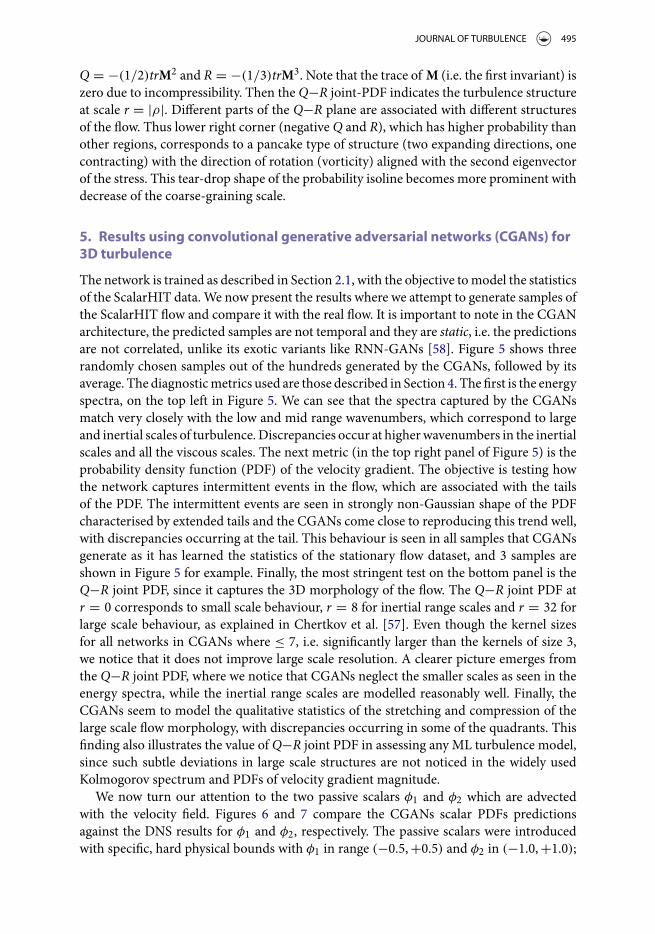
Q = −(1/2)trM2 and R = −(1/3)trM3. Note that the trace of M (i.e. the first invariant) iszero due to incompressibility. Then theQ−R joint-PDF indicates the turbulence structureat scale r = |ρ|. Different parts of the Q−R plane are associated with different structuresof the flow. Thus lower right corner (negative Q and R), which has higher probability thanother regions, corresponds to a pancake type of structure (two expanding directions, onecontracting) with the direction of rotation (vorticity) aligned with the second eigenvectorof the stress. This tear-drop shape of the probability isoline becomes more prominent withdecrease of the coarse-graining scale.

5. Results using convolutional generative adversarial networks (CGANs) for3D turbulence

The network is trained as described in Section 2.1, with the objective tomodel the statisticsof the ScalarHIT data. We now present the results where we attempt to generate samples ofthe ScalarHIT flow and compare it with the real flow. It is important to note in the CGANarchitecture, the predicted samples are not temporal and they are static, i.e. the predictionsare not correlated, unlike its exotic variants like RNN-GANs [58]. Figure 5 shows threerandomly chosen samples out of the hundreds generated by the CGANs, followed by itsaverage. The diagnosticmetrics used are those described in Section 4. The first is the energyspectra, on the top left in Figure 5. We can see that the spectra captured by the CGANsmatch very closely with the low and mid range wavenumbers, which correspond to largeand inertial scales of turbulence. Discrepancies occur at higherwavenumbers in the inertialscales and all the viscous scales. The next metric (in the top right panel of Figure 5) is theprobability density function (PDF) of the velocity gradient. The objective is testing howthe network captures intermittent events in the flow, which are associated with the tailsof the PDF. The intermittent events are seen in strongly non-Gaussian shape of the PDFcharacterised by extended tails and the CGANs come close to reproducing this trend well,with discrepancies occurring at the tail. This behaviour is seen in all samples that CGANsgenerate as it has learned the statistics of the stationary flow dataset, and 3 samples areshown in Figure 5 for example. Finally, the most stringent test on the bottom panel is theQ−R joint PDF, since it captures the 3D morphology of the flow. The Q−R joint PDF atr = 0 corresponds to small scale behaviour, r = 8 for inertial range scales and r = 32 forlarge scale behaviour, as explained in Chertkov et al. [57]. Even though the kernel sizesfor all networks in CGANs where ≤ 7, i.e. significantly larger than the kernels of size 3,we notice that it does not improve large scale resolution. A clearer picture emerges fromthe Q−R joint PDF, where we notice that CGANs neglect the smaller scales as seen in theenergy spectra, while the inertial range scales are modelled reasonably well. Finally, theCGANs seem to model the qualitative statistics of the stretching and compression of thelarge scale flow morphology, with discrepancies occurring in some of the quadrants. Thisfinding also illustrates the value of Q−R joint PDF in assessing any ML turbulence model,since such subtle deviations in large scale structures are not noticed in the widely usedKolmogorov spectrum and PDFs of velocity gradient magnitude.

We now turn our attention to the two passive scalars φ1 and φ2 which are advectedwith the velocity field. Figures 6 and 7 compare the CGANs scalar PDFs predictionsagainst the DNS results for φ1 and φ2, respectively. The passive scalars were introducedwith specific, hard physical bounds with φ1 in range (−0.5,+0.5) and φ2 in (−1.0,+1.0);


Figure 5. Energy spectra (top left), PDF of the longitudinal velocity gradient magnitude (top right), andjoint PDFs of the Q and R invariants of the coarse-grained velocity gradient tensor (bottom) for randomlychosen static snapshot predictions produced by CGANs


Figure 6. Normalised PDFs of passive scalars φ1 predicted by CGANs and comparison with DNS, whereCGANs fail to capture accurate scalar PDF bounds.

which is encountered in many physical scalars (e.g. mass fractions). We see that whileCGANs predictions for both scalars appear to capture the PDF profile, they severely over-shoot the scalar bounds, with the predicted φ1 and φ2 bounded between (−1.0,+1.0) and(−2.0,+2.0) respectively. Therefore, even though the convolutional generator can suffi-ciently learn trends of large-scale behaviour in the velocity fields, it appears that it hassevere difficulties learning the advected quantities by the same velocity fields, especially forhighly non-gaussian PDFs (as seen in Figure 7). This points to a topic worthy of furtherresearch due to the popularity of GANs in modelling turbulent velocity fields, with passivescalars having not been previously explored.

6. Analysis of 3D turbulence dimensionality reduction with convolutionalautoencoders

The schematic of the CAE architecture used for the ScalarHIT dataset is shown in Figure 9.The CAE greatly reduces the memory utilisation since the same n weights in a convolu-tional kernel are translated throughout the domain of size m × m, where m � n. Thesen weights are global, hence learned for all regions of the domain. In contrast, the stan-dard, fully-connected autoencoder architecture would need m2 weights which are local,leading to prohibitive memory consumption and extremely high training cost. In addi-tion to computational benefits, the design of the convolutional kernel offers flexibility in


Figure 7. Normalised PDFs of passive scalar φ2 predicted by CGANs and comparison with DNS, whereCGANs fail to capture accurate scalar PDF bounds.

tuning the number of shared weights and mode of translation through the domain, as willbe explained in this section.

Another important aspect is the number of features, i.e. trainable parameters in theCAE. In the case of ScalarHIT dataset, there are five features corresponding to the threecomponents of velocity and two passive scalars. Increasing the number of features in thelatent space allows it to encode more information at a minimal increase in computing cost,while also compressing the high dimensional dataset.We thus define the compression ratioz as

z = (original dimensions × number of input features)(latent dimensions × number of latent features)

(8)

From Equation (8), it follows that for input dimensions of size 1283 with 5 features; anda latent space of dimensions 153 with 25 features, there is considerably lesser impact onz with increase in latent space features. As such, the most significant impact comes fromthe latent space dimensions, giving us the liberty to increase the feature space. In fact, theCAE in this work uses 25 features to obtain a compression ratio of ≈ 125, i.e. a 125-folddecrease in size for every snapshot of the flow. This leads to tremendous gains in efficiencyandmakes aROMcomputationally efficient, since the original dimensionswere prohibitivefrom a memory standpoint. Mathematically, we can say that the subspace spanned by theinput features is mapped by a neural network onto a latent subspace spanned by a differentset of learned features. Typically, an increased number of features in the latent space hasa direct effect on accuracy of compression, but with a decrease in the compression ratio


Figure 8. Variable striding in convolutional kernels with kernel size α and stride length β : β = 1 cor-responds to cell by cell striding, while β = 3 skips over 2 cells for every stride, thereby producing aconvolved domain of lower dimension.

Figure 9. Schematic of a convolutional autoencoderNNArchitecturewith kernel sizeα and kernel strideβ for dimensionality reduction of input data to latent space, and reconstruction from reduced latentspace to original dimensions.

and increase in the computational cost. The optimal number of features is therefore a userchoice, based on compute resources and level of compression required. In any CAE, twokey design choices have to be made: the kernel size, α and kernel stride, β . The kernel sizeindicates the spatial extent of a single kernel. For instance, a kernel size of 3 × 3 × 3 con-tains 27 shared, trainable weights. The next choice is to decide how the shared weights (i.e.the kernel) translate across the domain. An illustration is shown in Figure 8, where a ker-nel α = 3 can be translated by a distance β of our choosing, known as stride. The figureshows kernel positions after β = 1 and β = 3 strides on the domain, and the strides arerepeated until the entire domain has been traversed by the kernel. By increasing the stride,the kernel needs fewer convolutions to cover the entire domain and results inmuch smallerdomain, as will be explained in the following section.

At the core of any CNN (and therefore a CAE) is the convolution operation. In theCAE encoder network (i.e. layers to the left of the latent space in the schematics), thekernel convolves with the data to reduce its dimensionality for every time instant ti. Asa result, a α = 3 kernel had dimensions (3 × 3 × 3) and therefore downsamples a spa-tial field of size 33 – known as the receptive field (Ref. [46]) – to a single point. Thedecoder network kernel (i.e. layers to the right of the latent space in the schematics) then


upsamples each point in the latent space back to the size of the receptive field througha deconvolution operation. Downsampling in the case of NNs can be explained as aweighted averaging operation, where the averaging weights are learned. Similarly, theupsampling kernel weights are also learned to perform the inverse operation. By stack-ing multiple CNN layers in the encoder, the input is downsampled in every layer andthe resulting domain – the latent space – can be extremely low dimensional. Likewise,upsampling can be performed by suitable number of decoding layers to recover the originaldimension.

It is important to note that dimensionality reduction to obtain an LDR is accompaniedby loss of some information. For instance, popular approaches like POD can representdominant energetic dynamics in the first few eigenpairs. These eigenpairs can be used forfurther analysis or modelling tasks, such as Galerkin projection, while the eigenpairs hav-ing very low energy contribution to the overall dataset are truncated, thereby leading toinformation loss. While the CAE is no exception, it distinguishes itself from the POD intwomajor ways: first, the POD bases compress the dataset as a linearmap, whereas autoen-coders with multiple layers and non-linear activation functions are inherently non-linearmaps [59]. Consequently, autoencoders can provide very high compression ratios for thesame dataset. Second, POD computation results in several global modes with the samedimensionality of the datasets, with ROMs primarily emulating only the temporal coeffi-cients of the modes, i.e. the spatial structures captured by the POD modes are still highdimensional. In contrast, CAE can directly learn local LDRs for each snapshot that havedegrees of freedom several orders of magnitude lower than the training dataset. From acomputing standpoint, this leads to significant reduction in memory resources and ROMscan now emulate both spatial and temporal dynamics with the low dimensional latentspace.

Since it is derived from a CNN, the information content learned by a CAE is dominatedby α and β . For a fixed kernel size α, the striding of the convolutional kernel has a directeffect on the dimensionality of the convolved output after each layer. From Figure 8, it isclear that increasing the stride diminishes the coverage of kernel over the domain, makingthe convolved output sparser. For a fixed α = 3, β = 3 leads to an overlap with receptivefield at the previous stride, while β = 3 removes any overlap. Higher values of β create gapsin the domain which are not seen by the kernel, and hence can traverse the entire domainin fewer steps than using β = 1. These choices significantly influence the accuracy, degreeof compression and computational cost of the ROM.We now present some physical insightabout α and β in the next section.

6.1. Physical interpretation of α and β

It is now worthwhile to discuss implications of the these choices in dimensionality reduc-tion of complex, spatio-temporal and multiscale datasets like turbulence. From the dis-cussion above, it is apparent that there are two competing strategies for dimensionalityreduction in a CAE. The first strategy relies on a large α to increase the receptive field.A larger receptive field would decompose several adjacent data-points into a single data-point. Therefore, for a desired dimension of the latent space, a suitable value of α can becomputed. The second strategy is to retain a constant, small α, but increase β to traversethe domain in as few steps as possible. The optimum β can be estimated from the desired


latent space dimension and the number of stacked layers we are willing to allow, due tocomputational cost involved in training deep networks.

There are caveats to both these strategies: A larger receptive field; in the limit of α → ∞(where ∞ refers to the dimensionality of the dataset) increases the number of trainableweights, with their number approaching the number of data-points in the domain. Asmen-tioned before, this is computationally prohibitive for 3D datasets of even small sizes and ishence not feasible. This leads to the second strategy of increasing β , while retaining a rel-atively small α. This also has pitfalls due to large discontinuities created between adjacentreceptive fields. A β = 1 leads to smooth transitions in convolution operations betweensubsequent layers, but requires large number of layers to achieve any meaningful dimen-sionality reduction. In contrast, β > 1 skips over some features in the domain, leading tosome information loss in the smaller scales. However, it also leads to significant dimension-ality reduction with fewer layers, which reduces computational costs. Figure 8 illustratesthe effect of these parameters on the convolution kernel. A β = 3 for α = 3 can quicklytraverse the domain in fewer steps, while a β = 1 for α = 3 ensures maximum overlapbetween adjacent receptive fields, at the cost of more traversal steps.

At this juncture, it is useful to develop some intuition on α and β in terms of numer-ical solution of partial differential equations in CFD. The convolutional kernel used inCAE has direct connections to the numerical stencils used in finite difference/finite vol-ume approaches [60,61]. Consider the standard second-order central difference scheme in1D for a quantity φ

φi−1 − 2φi + φi+1

δ2(9)

This can be represented as a 1D convolutional kernel of α = 3 with three constant weights1δ2, −2

δ2and 1

δ2. In the CAE, the kernel has the same structure, but all the constant weights

in the convolutional kernels are replaced with learnable weights. Therefore, the output oftrained kernel is analogous to aweighted combination of adjacent points, akin to numericalsolution of PDEs. In fact, there are deeper connections between convolutional kernels andstencils of numerical schemes that have been uncovered recently for developing efficientneural network based PDE solvers, and the reader is directed to the Long et al. [61] andDong et al. [60].

In numerical solutions of PDEs, the kernel size corresponds to the order of numericalscheme, which is typically constant and computed at every point in the domain. By anal-ogy, larger stencils may represent higher order numerical schemes, as seen by an increasednumber of trainable weights in networks. Extending the CNN terminology to PDE solversfor comparison, a PDE solver has a constant α and β = 1 which completes its operation ina single ‘layer’. In contrast, the CAE hasmultiple layers with flexibility to have differentα,βin each layer. Thus each layer of theCAE encoder consists of a customised numerical stencilspecific to the dataset. In lieu of these close connections, the practical differences betweenPDE solvers andCAEs boil down to the treatment of boundaries, stride and themapping ofinput features into a different subspace. In CAE, only the first layer in the deep neural net-work encoder treats the boundaries, while the increasing β at successive layers decreasesdimensionality of the data. In summary, CAE encoders map the high dimensional inputfeatures into a low dimensional latent space with an intelligent choice of kernel weights,kernel sizes and stride lengths. The CAE decoder is essentially an inverse operation of


the encoder, but not in an explicit, mathematically exact fashion [62]. Instead the decoderweights and strides are trained with the encoder to estimate the inverse map from latentspace to original data. These connections can be exploited to build CNNswith hard physicsconstraints based on numerical methods, and the reader is referred to Mohan et al. [63]for details.

6.2. Convolutional autoencoders: influence of kernel size and sequence length

The discussion thus far has emphasised the role of kernel size α, in a CNN (and there-fore, a CAE) as a hyper-parameter with important consequences on the accuracy of ourlearned model. In this work, each batch trained consists of snapshots that retain their tem-poral order and are not shuffled. This means the CAE has to extract a low dimensionallatent space from the dynamics of a temporal sequence, as opposed to learning from eachsnapshot as an independent sample. Consequently, the temporal gap between subsequentsnapshots, i.e. sampling-rate ω becomes a factor building a DL-based ROM.

We now seek to study if the accuracy of the learned latent space is sensitive to this rela-tionship. To understand the sensitivity of our model toω, we increase the sampling rate fora constant batch size, to account formany real-world applicationswhere data collection fre-quency is not ideal. Since the kernel performs a convolution operation over a numericalgrid, its receptive field is intimately connected to the turbulence scales it captures. Intu-itively, we would expect larger kernel sizes to capture spatial correlations of larger scales.Likewise, it follows that these kernels would also capture dynamics over longer time scales,due to the relationship between length and time scales in turbulence. By decreasing thesampling rate of the snapshots, we can account for these longer temporal scales, while keep-ing the batch size same. This ensures that all the differences we observe in model accuracyis not from the batch size, but rather its sampling frequency.

We intend to experimentally quantify the influence of α on the accuracy of the compres-sion, for future applications in 3D turbulence. The goal is to observe if turbulent featuresover a range of scales orders of magnitudes apart, show any preferential dependence tolearning by various kernel sizes and sampling rates. We choose ω to be 3, 6 and 9 samplesapart, which corresponds to ω = 0.09τ , 0.18τ and 0.27τ , where τ is the eddy turnovertime for this flow. Finally, such a hyper-parameter sweep would seek to establish that theresults are consistent, and not due to chance numerical artefacts that may have occurredduring optimisation. To this end, several experiments are performed with two families ofparameters:

(1) With a small kernel size α = 3, vary sampling rate as ω = 0.09τ , 0.18τ , 0.27τ .(2) With large kernel size α = 9, vary sampling rate as ω = 0.09τ , 0.18τ , 0.27τ .

For consistency, we ensure that the number of layers and the striding β in the encoderand decoder are constant for all experiments. The α = 9 kernel creates a higher compres-sion ratio than α = 3, for the same number of layers in encoder and decoder. As a result,the only variables in the experiments are α and ω. All experiments above are also trainedwith three commonly used optimisers – Adam [64], Adadelta [65] and RMSProp [66] andthe best model is used for analysis, to ensure the final trends are not a consequence ofan arbitrary choice of optimiser, but instead an outcome of the α and ω choices. We now


present the results, and the trained model is assessed using the same diagnostic metricsmentioned in Section 4. All the diagnostics compare the statistics generated from (a) DNSsnapshots and (b) CAE reconstructedmodels of their corresponding latent states. The pre-vious discussion in Section 6.1 points to information loss in small scale behaviour due toβ > 1. Quantifying the accuracy of the latent space with these physics based diagnosticswill shed light if this indeed holds true.

6.2.1. Convolutional autoencoder: α = 3The statistical diagnostics for the small kernel α = 3 withω = 0.09τ is shown in Figure 10.To indicate the quality of the model, we show diagnostics at three randomly chosen sam-ples, followed by the averaged diagnostics for several samples. We adopt this style for allCAE results in this work. From the energy spectra, it is clear that large and inertial rangefrequencies are retained accurately, while there is a marked discrepancy in the small scalefrequencies. This behaviour is also observed in the velocity gradient PDFs, where the largescale events around Z = 0 are well resolved, while discrepancies corresponding to smallscales exist at the tails. Finally, the most stringent test is the Q−R plane PDF, since it cap-tures the 3Dmorphology of the flow. TheQ−R spectra at r = 0 corresponds to small scalebehaviour, r = 8 for inertial range scales and r = 32 for large scale behaviour. The spec-tra shows excellent agreement at large scales, thereby corroborating the results from theenergy spectra. The structure of the inertial range is also accurately captured, with veryminor discrepancies in stretching behaviour. Finally, we see that the small scale behaviouris almost entirely neglected by the kernel. The symmetric nature of PDFs indicates thatthe network may be generating some random noise to compensate for information lossin the small scales. Interestingly, the discussion about β and its relationship to turbulencescales in the previous section indicates this outcome, which we have now verified. We nowdiscuss the sensitivity of training with ω. The sampling rate is progressively decreased toω = 0.09τ , 0.18τ and the diagnostics are shown in Figures 11 and 12 respectively. Thediagnostics show that the quality of results are extremely robust despite a decrease in tem-poral sampling rate of the data. We caution that this may likely be true only for cases likestationary, homogeneous turbulence, whereas accuracy for flowswith strong transients andnon-stationarity can be affected by ω.

6.2.2. Convolutional autoencoder: α = 9We now turn our attention to the large kernel α = 9 with ω = 0.09τ . The diagnostics inFigure 13 paint a somewhat different picture in comparison with the small kernel. Theenergy spectra shows good agreement in the low wavenumbers, but gets progressivelyworse with increasing wavenumber. Finally, the high wavenumbers show major discrep-ancies with oscillatory behaviour not present in the DNS dataset. On the other hand, thevelocity gradient PDFs show a much better agreement with the DNS than the small ker-nel. This seemingly counter-intuitive behaviour likely happens due to the random highwavenumber oscillations (seen in the energy spectra) fortuitously replicating averagedsmall scale intermittent fluctuations in DNS. Finally, we get a clear understanding of thelarge kernel performance looking at theQ−R PDF statistics. The statistics show good largescale reconstruction, but significant discrepancies in the inertial range, with the somewhatsymmetric stretching in theR axis implying addition of randomnoise to the lower quadrantof the Q−R plane. The noise effect is further accentuated in the small scale statistics, with


Figure 10. Energy spectra (top left), PDFof the longitudinal velocity gradientmagnitude (top right), andjoint PDFs of the Q and R invariants of the coarse-grained velocity gradient tensor (bottom) for randomlychosen samples from CAE-NN dimensionality reduction with α = 3 andω = 0.09τ .












appreciable deviations from the DNS statistics. Similar to the small kernel, experiments arealso performed for ω = 0.09τ , 0.18τ and the diagnostics are shown in Figures 14 and 15respectively. For ω = 0.18τ we see similar behaviour as ω = 0.09τ , except for minor dis-crepancies in the large scales. These trends are repeated in ω = 0.27τ . Overall, the qualityof reconstruction does not seem to change with decreasing sampling frequency, as seenfor α = 3. Furthermore, all the results show consistent addition of random noise to highwavenumbers and several inertial-range wavenumbers. The presence of noise in the largekernel happens to be the most significant difference from the small kernel, which conse-quently leads to deterioration in reconstruction. It bears mentioning that the large kernelcontains more parameters than the small kernel, and as such needs significantly longertraining time to obtain convergence. In this work, the training time for α = 9 was twicethat of α = 3, and the memory requirements were considerably higher.

From these experiments we can conclude that, at least for the case of isotropic turbu-lence, the kernel size appears to be a more important parameter affecting model accuracythan the sampling rate of the data. We note that while a large kernel is capable of highercompression ratios than a small kernel for the same layers, it comes at the price of accuracy,computational time and memory. While both large and small kernels capture large scalebehaviour well, the small kernel also reconstructs the inertial scales reasonably well.

7. Results using compressed convolutional LSTM (CC-LSTM)

As discussed previously, the ConvLSTMnetwork (Figure 2) necessitates some form of datacompression to efficiently learn the spatio-temporal dynamics of the flow with tractablecomputational effort. The CAEs described above are seen to learn efficient latent spacerepresentations of the flow with excellent compression in data size, and we denote thecombined approach as CC-LSTM. As mentioned in Section 3, we use as training datathe time-varying latent space for τ = 3 snapshots. After the parametric study with dif-ferent α and ω, it is observed that α = 3 and ω = 0.09τ learn sufficiently accurate modelswith the lowest computational cost. Therefore, we use the latent space models from thisconfiguration as the ConvLSTM training data.

Since a ConvLSTM network can model spatio-temporal dynamics, we evaluate it bymaking continuous predictions in time. We give a batch of temporal flow snapshots com-pressed into CAE latent spaces as input and the network predicts the next batch of latentspaces evolved in time. These predicted latent spaces are then used to recover the truedimensions of the flow thru the CAE decoder. The model is autoregressive, since the pre-dictions are fed back into the network as a new input.We repeat this autoregressive processfor several time instants, to study both the accuracy of the predicted snapshots, and how farin time the network is able to generate stable snapshots without significant deterioration inaccuracy. The diagnostic tests outlined in Section 4 are used to evaluate CC-LSTM gener-ated snapshots. The velocity diagnostics are shown in Figure 16 for predicted snapshots at1.5 eddy times from τ = 3 − 4.5 in the DNS dataset. We make autoregressive predictionsin τ ∗ = τ − 3 = 0 → 1.5, and the diagnostics are shown for τ ∗ = 0.1, 1.0, 1.5 such that weare evaluating temporally correlated snapshots across the predicted range. The ConvLSTMnetwork has 3 layers with constant kernel size α = 3, with each hidden cell having 40 fea-tures and RMSProp optimiser used to train the network. The approach was implementedusing the Pytorch [67] framework and trained in a distributed multi-GPU batch-parallelfashion.


Figure 16. Energy spectra (top left), PDF of the longitudinal velocity gradient magnitude (top right),and joint PDFs of the Q and R invariants of the coarse-grained velocity gradient tensor (bottom). CC-LSTM predictions are more accurate than CGANs and temporally stable, with errors concentrated in thesmall scales.


Figure 17. Instantaneous φ1 scalar PDFs bounded [−0.5,+0.5] from DNS and NN at different timeinstances: τ ∗ = 0.1 (top), τ ∗ = 1.0 (middle), τ ∗ = 1.5 (bottom). CC-LSTM predictions are bounded andmore accurate than CGANs with minor discrepancies at tails.


Figure 18. Instantaneous φ2 scalar PDFs bounded [−1.0,+1.0] from DNS and NN at different timeinstances: τ ∗ = 0.1 (top), τ ∗ = 1.0 (middle), τ ∗ = 1.5 (bottom). CC-LSTM predictions are bounded andmore accurate than CGANs with minor discrepancies at tails.


We see from the energy spectra that the large scale and inertial range spectra are pre-dicted extremely well, with discrepancies only in the small scale range. Interestingly, thevelocity gradient PDFs show near-perfect resolution across all the scales, including thesmall scale behaviour at the tails. This likely indicates the ConvLSTM network is addingsome artefacts to the predictions which accurately mimics the tail behaviour of the PDF,since this was not a condition we enforced on the network. A more rigorous evaluation isperformed with the Q−R PDFs, where we see that the statistical trends of the small scalesare neglected by the network as expected. Furthermore, we see that the large scale trends arepredicted quite well, followed by inertial range scales with some discrepancies. Typically,most temporal modelling techniques are accompanied by a significant loss in accuracy asthe prediction horizon τ ∗ increases. In this case, we see onlymarginal deterioration in largescale statistics at τ ∗ > 1. The loss of accuracy is somewhat more significant in the inertialscales, while the small scales do not seemuch change. From these diagnostics, it is apparentthat the CC-LSTM is able to consistently model large scale velocity dynamics of ScalarHITover extended time ranges, even while the accuracy in other scales might suffer. This isquite promising, since modelling large scale dynamics at high fidelity is a requirement forseveral practical applications.

We now turn our attention to the passive scalars. Figure 17 compares PDFs of theDNS and CC-LSTM predictions at τ ∗ = 0.1, 1.0, 1.5 for the scalar φ1. We observe that thepredicted scalar is generally accurate and well bounded in (−0.5, 0.5) with only a minorovershoot. This is also observed in the predictions of scalar φ2 in Figure 18, where the net-work not only captures the PDF, but also tries to retain boundedness. These results showthat the CC-LSTM are able to outperform CGANs in predicting both velocity vectors andpassive scalars despite loss of information arising from the autoencoders.

Finally, a key factor to evaluate these architectures is the computational resourcesrequired to train an ROM. Since the CC-LSTM primarily learns dynamics on latent spacerather than the high dimensional raw data, it requires orders of magnitude fewer parame-ters than CGANs, which has generally been the more popular approach in the turbulencecommunity. The details of the computational costs are outlined in Appendix A.5, andshow significant advantages of CC-LSTM over CGANs when scaling these approaches tolarge, realistic flows. Furthermore, we note that training GANs/CGANs in a stable man-ner involves several modifications over hyper-parameters in both the network design andoptimisation, and has been well documented elsewhere in the broader machine learningliterature [32,68–70]. In this work, the authors had to implement several strategies out-lined in Appendix A.2 to obtain reliable predictions using CGANs. In contrast, CC-LSTMtraining was markedly more stable and resilient to variations in hyper-parameter choicesacross different kernel sizes and sequence lengths, further reducing compute cost.

8. Conclusion

In this work, we report a first systematic study of deep learning strategies for the generationof fully developed three-dimensional turbulence.We evaluate neural network architecturesrepresenting two different approaches to high-dimensional data modelling. The quality ofthe deep learning predictivemodels is tested with physics-basedmetrics which identify thestatistical characteristics of 3D turbulence. The first architecture is a 3D convolutional vari-ant of popular approach known as Generative Adversarial Networks (GANs). In this work,


ConvolutionalGANs (CGANs) are demonstrated to have acceptable accuracy inmodellinglarge and inertial scale velocity features of individual snapshots of the flow, albeit withoutcapability for temporal predictions. However, we also notice CGANs difficulties in mod-elling the probability density functions (PDFs) of the passive scalars advected with thevelocity, with the predictions being frequently unbounded. Since CGANs lack temporaldynamics, we propose an alternative neural network approach to perform spatio-temporalprediction. This novel strategy utilises a convolutional autoencoder (CAE) neural networkfollowed by a Convolutional LSTM (ConvLSTM) network. The CAE learns a projectionof the high-dimensional spatial data to a low dimensional latent space, such that the latentspace can be used as an input for temporal predictions. We then employ the ConvLSTMnetwork to predict the latent space at future time instants. This two-tier prediction model,coined Compressed Convolutional LSTM (CC-LSTM), is able to predict dynamics of theflow. Furthermore, the CC-LSTM allows accurate reproduction of the large and inertialscale statisticsmaking it very attractive formany practical/engineering applications. In caseof the passive scalars, the CC-LSTM is able to capture the PDFs accurately, while bound-ing the scalar PDFs within its theoretical limits with only minor overshoot, as opposed toCGANs. From a practical standpoint, one of the major observations of this investigationis significant disparity between computational efficiency of CC-LSTM, when comparedwith popular, state-of-the art approaches like CGANs, in the context of 3D turbulence.Due to large number of parameters that ConvLSTM networks need even for modestlysized datasets, we show that performing model reduction with CAEs is a valuable first stepin computationally efficient learning models of 3D turbulence. This modified CC-LSTMapproach needs orders ofmagnitude fewer trainable parameters than CGANs, while show-ing superior spatio-temporal predictive accuracy. While the networks shown in this workdo not have explicit physics constraints, versions of autoencoders with hard constraintsdemonstrated by the authors in [63] can be easily adapted to the CC-LSTM framework,providing considerable flexibility in learning.

Acknowledgements

The authors thank Don Daniel (LANL) for the dataset and valuable discussions. This workhas been authored by employees of Triad National Security, LLC, which operates Los AlamosNational Laboratory (LANL) underContractNo. 89233218CNA000001with theU.S.Department ofEnergy/National Nuclear Security Administration. A.T.M. and D.L. have been supported by LANL’sLDRD program, project number 20190058DR. A.T.M. also thanks the Center for Nonlinear Stud-ies at LANL for support and acknowledges the ASC/LANL Darwin cluster for GPU computinginfrastructure.

Disclosure statement

No potential conflict of interest was reported by the author(s).

Funding

This work was supported by U.S. Department of Energy [LDRD Los Alamos National Laboratory].

ORCID

Arvind T. Mohan http://orcid.org/0000-0002-9434-7691

http://orcid.org/0000-0002-9434-7691


References

[1] Wu JL, Xiao H, Paterson E. Physics-informed machine learning approach for augmentingturbulence models: a comprehensive framework. Phys Rev Fluids. 2018;3(7):074602.

[2] Wang JX, Wu J, Ling J, et al. A comprehensive physics-informed machine learning frameworkfor predictive turbulence modeling. Preprint arXiv:170107102. 2017.

[3] Tracey BD, Duraisamy K, Alonso JJ. A machine learning strategy to assist turbulence modeldevelopment. In: Proceedings of the 53rd AIAA Aerospace Sciences Meeting; Kissimmee,Florida, Publisher: AIAA (American Institute of Aeronautics and Astronautics), 2015. p. 1287.

[4] Singh AP, Medida S, Duraisamy K. Machine-learning-augmented predictive modeling ofturbulent separated flows over airfoils. AIAA J. 2017;55(7):2215–2227.

[5] Maulik R, San O, Rasheed A, et al. Subgrid modelling for two-dimensional turbulence usingneural networks. J Fluid Mech. 2019;858:122–144.

[6] Ling J, Kurzawski A, Templeton J. Reynolds averaged turbulence modelling using deep neuralnetworks with embedded invariance. J Fluid Mech. 2016;807:155–166.

[7] Klein M, Sadiki A, Janicka J. A digital filter based generation of inflow data for spatiallydeveloping direct numerical or large eddy simulations. J Comput Phys. 2003;186(2):652–665.

[8] Di Mare L, Klein M, Jones W, et al. Synthetic turbulence inflow conditions for large-eddysimulation. Phys Fluids. 2006;18(2):025107.

[9] Juneja A, Lathrop D, Sreenivasan K, et al. Synthetic turbulence. Phys Rev E. 1994;49(6):5179.[10] Jarrin N, Benhamadouche S, Laurence D, et al. A synthetic-eddy-method for generating inflow

conditions for large-eddy simulations. Int J Heat Fluid Flow. 2006;27(4):585–593.[11] RempferD.On low-dimensional galerkinmodels for fluid flow. Theoret Comput FluidDynam.

2000;14(2):75–88.[12] Noack BR, Papas P, Monkewitz PA. The need for a pressure-term representation in empirical

Galerkin models of incompressible shear flows. J Fluid Mech. 2005;523:339–365.[13] Carlberg K, Bou-Mosleh C, Farhat C. Efficient non-linear model reduction via a least-squares

Petrov–Galerkin projection and compressive tensor approximations. Int J Numer MethodsEng. 2011;86(2):155–181.

[14] Qian E, Kramer B, Peherstorfer B, et al. Lift & learn: physics-informed machine learning forlarge-scale nonlinear dynamical systems. Phys D Nonlinear Phenomena. 2020;406:132401.

[15] Deshmukh R, McNamara JJ, Liang Z, et al. Model order reduction using sparse codingexemplified for the lid-driven cavity. J Fluid Mech. 2016;808:189–223.

[16] Sargsyan S, Brunton SL, Kutz JN. Nonlinear model reduction for dynamical systems usingsparse sensor locations from learned libraries. Phys Rev E. 2015;92(3):033304.

[17] Kaiser E, Noack BR, Cordier L, et al. Cluster-based reduced-order modelling of a mixing layer.J Fluid Mech. 2014;754:365–414.

[18] Nair AG, Taira K. Network-theoretic approach to sparsified discrete vortex dynamics. J FluidMech. 2015;768:549–571.

[19] Goodfellow I, Pouget-Abadie J, Mirza M. Generative adversarial nets. In: Proceedings ofthe Advances in Neural Information Processing Systems; 2014, Montreal, Canada. Publisher:Neural Information Processing Systems, p. 2672–2680.

[20] Xingjian S, Chen Z, Wang H. Convolutional lstm network: a machine learning approach forprecipitation nowcasting. In: Proceedings of the Advances in Neural Information Process-ing Systems; Montreal, Canada. Publisher: Neural Information Processing Systems, 2015. p.802–810.

[21] Chu M, Thuerey N. Data-driven synthesis of smoke flows with cnn-based feature descriptors.ACM Trans Graphics (TOG). 2017;36(4):69.

[22] UmK,HuX, ThuereyN. Liquid splashmodelingwith neural networks. In: ComputerGraphicsForum, Vol. 37. Wiley Online Library; 2018. p. 171–182.

[23] Mukherjee R, Li Q, Chen Z, et al. NeuraldropDnn-based simulation of small-scale liquid flowson solids. Preprint arXiv:181102517. 2018.

[24] Zimmermann RS, Parlitz U. Observing spatio-temporal dynamics of excitable media usingreservoir computing. Chaos: An Interdisciplinary J Nonlinear Sci. 2018;28(4):043118.


[25] LuZ, Pathak J,Hunt B, et al. Reservoir observers:model-free inference of unmeasured variablesin chaotic systems. Chaos Interdisc J Nonlinear Sci. 2017;27(4):041102.

[26] Pathak J, Wikner A, Fussell R, et al. Hybrid forecasting of chaotic processes: using machinelearning in conjunction with a knowledge-based model. Chaos Interdisc J Nonlinear Sci.2018;28(4):041101.

[27] Pathak J, Hunt B, Girvan M, et al. Model-free prediction of large spatiotemporally chaoticsystems from data: a reservoir computing approach. Phys Rev Lett. 2018;120(2):024102.

[28] Wu JL, Kashinath K, Albert A, et al. Enforcing statistical constraints in generative adversarialnetworks for modeling chaotic dynamical systems. Preprint arXiv:190506841. 2019.

[29] King R, Hennigh O, Mohan A, et al. From deep to physics-informed learning of turbulence:diagnostics. Preprint arXiv:181007785. 2018.

[30] Yang Z,Wu JL, XiaoH. Enforcing deterministic constraints on generative adversarial networksfor emulating physical systems. Preprint arXiv:191106671. 2019.

[31] Chen W, Chiu K, Fuge M. Aerodynamic design optimization and shape exploration usinggenerative adversarial networks. In: Proceedings of the AIAA Scitech 2019 Forum. 2019, SanDiego, California. Publisher: AIAA (American Institute of Aeronautics and Astronautics), p.2351.

[32] Radford A, Metz L, Chintala S. Unsupervised representation learning with deep convolutionalgenerative adversarial networks. Preprint arXiv:151106434. 2015.

[33] Ioffe S, Szegedy C. Batch normalization: accelerating deep network training by reducinginternal covariate shift. e-prints. arXiv:1502.03167. 2015 Feb.

[34] Che T, Li Y, Jacob AP, et al. Mode regularized generative adversarial networks. PreprintarXiv:161202136. 2016.

[35] Salimans T, Goodfellow IJ, Zaremba W, et al. Improved techniques for training gans. CoRR.2016. abs/1606.03498. http://arxiv.org/abs/1606.03498.

[36] Deng L. The mnist database of handwritten digit images for machine learning research [bestof the web]. IEEE Signal Process Mag. 2012;29(6):141–142.

[37] Holmes PJ, Lumley JL, Berkooz G, et al. Low-dimensional models of coherent structures inturbulence. Phys Rep. 1997;287(4):337–384.

[38] Mezić I. Analysis of fluid flows via spectral properties of the Koopman operator. Annu RevFluid Mech. 2013;45:357–378.

[39] Bagheri S. Koopman-mode decomposition of the cylinder wake. J Fluid Mech. 2013;726:596–623.

[40] Rowley CW, Mezić I, Bagheri S, et al. Spectral analysis of nonlinear flows. J Fluid Mech.2009;641:115–127.

[41] Lusch B, Kutz JN, Brunton SL. Deep learning for universal linear embeddings of nonlineardynamics. Nat Commun. 2018;9(1):4950.

[42] Yeung E, Kundu S, Hodas N. Learning deep neural network representations for koopmanoperators of nonlinear dynamical systems. Preprint arXiv:170806850. 2017.

[43] Sirisup S, Karniadakis GE. A spectral viscosity method for correcting the long-term behaviorof pod models. J Comput Phys. 2004;194(1):92–116.

[44] Mohan AT, Gaitonde DV. A deep learning based approach to reduced order modeling forturbulent flow control using LSTM neural networks. Preprint arXiv:180409269. 2018.

[45] Theis L, ShiW,CunninghamA, et al. Lossy image compressionwith compressive autoencoders.Preprint arXiv:170300395. 2017.

[46] Goodfellow I, Bengio Y, Courville A. Deep learning. MIT Press; 2016.[47] Qi CR, Su H, Nießner M. Volumetric and multi-view cnns for object classification on 3d data.

In: Proceedings of the IEEE Conference on Computer Vision and Pattern Recognition; LasVegas, Nevada. Publisher: IEEE 2016. p. 5648–5656.

[48] Luong MT, Manning CD. Stanford neural machine translation systems for spoken languagedomains. In: Proceedings of the International Workshop on Spoken Language Translation;2015, DaNang, Vietnam. Publisher: InternationalWorkshop on Spoken Language Translation.p. 76–79.

http://arxiv.org/abs/1606.03498


[49] Nelson DM, Pereira AC, de Oliveira RA. Stock market’s price movement prediction withlstm neural networks. In: Proceedings of the 2017 International Joint Conference on NeuralNetworks (IJCNN). IEEE; 2017.Anchorage, Alaska p. 1419–1426.

[50] WuH, Prasad S. Convolutional recurrent neural networks forhyperspectral data classification.Remote Sens (Basel). 2017;9(3):298.

[51] Zhu G, Zhang L, Shen P, et al. Multimodal gesture recognition using 3-d convolution andconvolutional lstm. IEEE Access. 2017;5:4517–4524.

[52] Zhao R, Yan R, Wang J, et al. Learning to monitor machine health with convolutionalbi-directional lstm networks. Sensors. 2017;17(2):273.

[53] Daniel D, Livescu D, Ryu J. Reaction analogy based forcing for incompressible scalar turbu-lence. Phys Rev Fluids. 2018;3(9):094602.

[54] Cook AW, Dimotakis PE. Transition stages of Rayleigh–Taylor instability between misciblefluids. J Fluid Mech. 2001;443:69–99.

[55] Livescu D, Ristorcelli J. Variable-density mixing in buoyancy-driven turbulence. J Fluid Mech.2008;605:145–180.

[56] Frisch U. Turbulence: the legacy of a. n. kolmogorov. Cambridge University Press; 1995.[57] Chertkov M, Pumir A, Shraiman BI. Lagrangian tetrad dynamics and the phenomenology of

turbulence. Phys Fluids. 1999;11(8):2394–2410.[58] Mogren O. C-rnn-gan: continuous recurrent neural networks with adversarial training.

Preprint arXiv:161109904. 2016.[59] Gonzalez FJ, Balajewicz M. Deep convolutional recurrent autoencoders for learning low-

dimensional feature dynamics of fluid systems. Preprint arXiv:180801346. 2018.[60] Dong B, Jiang Q, Shen Z. Image restoration wavelet frame shrinkage, nonlinear evolution

PDES, and beyond. Multiscale Model Simul. 2017;15(1):606–660.[61] Long Z, Lu Y, Ma X, et al. Pde-net: learning pdes from data. Preprint arXiv:171009668. 2017.[62] Ardizzone L, Kruse J, Wirkert S, et al. Analyzing inverse problems with invertible neural

networks. Preprint arXiv:180804730. 2018.[63] MohanAT, LubbersN, LivescuD, et al. Embedding hard physical constraints in neural network

coarse-graining of 3d turbulence. Preprint arXiv:200200021. 2020.[64] Kingma DP, Ba J. Adam: a method for stochastic optimization. Preprint arXiv:14126980. 2014.[65] Zeiler MD. Adadelta: an adaptive learning rate method. Preprint arXiv:12125701. 2012.[66] Tieleman T, Hinton G. Lecture 6.5-rmsprop divide the gradient by a running average of its

recent magnitude. COURSERA: Neural Networks for Machine Learning. 2012;4(2):26–31.[67] Paszke A, Gross S, Massa F. Pytorch: an imperative style, high-performance deep learning

library. In: Advances in Neural Information Processing Systems; 2019.Vancouver, Canada,Publisher: Neural Information Processing Systems p. 8024–8035.

[68] Thanh-Tung H, Tran T, Venkatesh S. Improving generalization and stability of generativeadversarial networks. Preprint arXiv:190203984. 2019.

[69] Arora S, Ge R, Liang Y. Generalization and equilibrium in generative adversarial nets (gans).In: Proceedings of the 34th International Conference on Machine Learning, Vol 70; JMLR.org; Sydney, Australia. Publisher: International Machine Learning Society 2017. p. 224–232.

[70] Arora S, Risteski A, Zhang Y. Do gans learn the distribution? some theory and empirics. ICLR;2018 Vancouver, Canada. Publisher: International Conference on Representation Learning.

[71] Hochreiter S. The vanishing gradient problem during learning recurrent neural nets and prob-lem solutions. Internat J Uncertain Fuzziness and Knowledge-Based Syst. 1998;6(02):107–116.

[72] Hochreiter S, Schmidhuber J. Long short-term memory. Neural Comput. 1997;9(8):1735–1780.

[73] Odena A, Dumoulin V, Olah C. Deconvolution and checkerboard artifacts. Distill; 2016.Available from: http://distill.pub/2016/deconv-checkerboard.

[74] Goodfellow I. Nips 2016 tutorial: generative adversarial networks. 2016. Available from:http://arxiv.org/abs/1701.00160.

[75] Smith LN. Cyclical learning rates for training neural networks. In: Proceedings of the 2017IEEE Winter Conference on Applications of Computer Vision (WACV); IEEE; 2017. p.464–472.

http://distill.pub/2016/deconv-checkerboard

http://arxiv.org/abs/1701.00160


Appendices

Appendix 1. Overview of neural network architectures

Artificial Neural networks (ANNs) can be broadly defined as a class of biologically inspired statis-tical representations which capture patterns and connections in a dataset. The elementary unit ofan ANN is the artificial neuron, and a layer of an ANN consists of multiple neurons. Subsequently,‘Deep’ ANNs are built by stacking multiple such layers one after the other. Mathematically, stackingnumerous neurons in a connectedmanner (often ranging fromhundreds tomillions) is able to repre-sent complex nonlinear functions, i.e. ANNs can universally approximate any function; which is theparadigmbehind the rise of themodern ‘deep learning’ revolution. Themathematical representationof a neuron is shown in Equation (A1)

y = φ

⎛⎝ m∑

j=0wkjxj

⎞⎠ (A1)

where x is the vector of inputs, withw being the series of ‘weights’ that produce the output y. The rightside of the equation is operated upon by an activation function φ, which can be nonlinear. The keyidea behind ANNs is that the weights w can be learned or estimated, given x and y. This is typicallyaccomplished by the backpropagation algorithm which iteratively computes w for any x−y pair viaoptimisation (usually gradient descent)-based methods. This process is broadly termed as trainingan ANN. While the core strategy of having learnable weights estimated with backpropagation andoptimisation methods have been the mainstay of deep learning, the actual architecture of the ANNhas greatly evolved. Specifically, these variations have focused on the structure and layout ofw, suchthat they are tailor-made for specific applications. Most applications can be broadly grouped intotwo classes of prediction problems: (a) classification and (b) regression. Classification problems areoften found in large image datasets; arising from satellite imagery, consumer devices and even sci-entific observations. Likewise, regression problems are ubiquitous in financial markets, consumerdemand forecasting, weather forecasting, and numerous scientific applications. Thus most of themodern architectures in deep learning have adapted the standard ANN layout of w to account forthese classes, which we will now outline.

A.1. Convolutional neural networks

Classification problems for image and other spatially varying datasets are difficult due to the largenumber of degrees of freedom. For instance, a 256 × 256 image has 65, 536 datapoints. The ANNhas all neurons connected to every other neuron, known as a fully connected NN or FCNN. It isimmediately apparent that training an FCNN for 65, 536 points requires atleast as many parame-ters, if not more. Therefore, FCNNs for images can be computationally prohibitive. However, weknow that images often have spatial correlations, so treating each datapoint in isolation may not bevery accurate (or efficient). As such, Convolutional Neural Networks (CNNs) are a class of ANNsdeveloped which exploits the fact that each point in an image is likely related to its neighbouringpoints. The w are structured as a kernel which translates throughout the image. The kernel is essen-tially a function that performs a convolution operation over the image data, and the result is trainedusing backpropagation. Therefore, instead of learning w for each individual point in the image, welearn w in a kernel with a predetermined size. This kernel can be used to extract patterns in otherimages. CNNs are often the driving force behind several state of the art image and pattern recogni-tion problems, and the idea of training a single kernel instead of an FCNN leads to drastic reductionsin computational cost.

A.2. Recurrent neural networks

Sequence prediction is different from other types of learning problems, since it imposes an order onthe observations that must be preserved when training models and making predictions. Recurrent


Neural Networks (RNNs) are a class of neural networks specially designed for such problems, whichpreserve this sequential information in the function being learned. A key assertion behind Recur-rent networks is that sequential processes have ‘memory’, i.e. the value of the process is a functionof the value at previous instants. Recurrent networks attempt to capture this sequential relationshipand learn the memory effects. The Long Short-Term Memory (LSTM) neural network is a specialvariant of RNN, which overcomes stability bottlenecks encountered in traditional RNNs (like theVanishing Gradient problem [71]), enabling its practical application. LSTMs can also learn and har-ness sequential dependence from the data, such that the predictions are conditional on the recentcontext in the input sequence. For instance, to predict the realisation at time ti, LSTMs can learnfrom the data at ti−1 and also at times ti−k, where k can be any number signifying the length ofthe prior sequence. In effect, k represents the ‘memory’ in the system, i.e. the extent to which theoutcome of the system depends on its previous realisations.

The basic architecture of the LSTM NN is now outlined. The LSTM networks are different fromother deep learning architectures like convolutional neural networks (CNNs), in that the typicalLSTM cell contains three gates: The input gate, output gate, and the forget gate. The LSTM regulatesthe flow of training information through these gates by selectively adding information (input gate),removing (forget gate) or letting it through to the next cell (output gate). A schematic of the cellsconnected in a recurrent form is shown in Figure A1.

The input gate is represented by i, output gate by o and forget gate by f. The cell state is representedas C and the cell output is given by h, while the cell input is denoted as x. Consider the equationsof an LSTM cell to compute its gates and states in Equation (A2) and a schematic of its structure inFigure A2.

ft = σ(Wf · [ht−1, xt] + bf

)it = σ (Wi · [ht−1, xt] + bi)

C̃t = tanh (WC · [ht−1, xt] + bC)

Ct = ft ∗ Ct−1 + it ∗ C̃t

ot = σ (Wo · [ht−1, xt] + bo)

ht = ot ∗ tanh (Ct)

(A2)

W are the weights for each of the gates and C̃ is the updated cell state. These states are propagatedahead through the network, as shown in Figure A1 and weights are updated by backpropagationthrough time. The forget gate plays a crucial role in reducing over-fitting by not retaining all infor-mation from the previous time steps. This arrangement of gates and selective information control isalso the key reason why LSTMs do not suffer from the vanishing gradient problem which plaguedtraditional RNNs [71]. As a result, LSTMs are a powerful tool to model sequential datasets. A moredetailed and introduction to LSTM can be found in Ref. [72].

Figure A1. LSTM layout with cell connections.


Figure A2. Architecture of an LSTM cell with various gates.

Appendix 2. CGANs: training and implementational details

The CGANs were trained with 96 feature maps each in both the generator and discriminator, with abatch size of 12. The noise vector to initialise the training was of size 100 × 1. A binary cross entropyloss with ADAM optimiser was used for training both the networks in GAN. The learning rate wasset at 2 × 10−5, with β1 = 0.5 and β2 = 0.999 being the optimisation parameters for ADAM.

A.3. Transpose convolution and resize convolution

Transpose convolutions are the traditional approach to upsampling used in CNN-based GANs. Thisoperation can be thought of as the reverse of a standard convolution: Instead of sliding a kernelacross a group of pixels to learn a mapping to fewer pixels, the kernel is trained to extrapolate indi-vidual pixels to a larger pixel group. The distance that the kernel slides each time is known as thestride. Deconvolution is sometimes mentioned as the same operation even though the two opera-tions are not the same (deconvolution is, technically, the inverse of convolution). Sincewe are dealingwith volumetric data, we utilise 3D transpose convolutions which use a cubic kernel. Furthermore,the stride defines how far the kernel translates each step, while the padding determines how manyzero-value pixels are added to the input. See Figure A3 for a comparison of 3D and 2D transposeconvolution. The use of transpose convolutions in the generator results in a common issue of GANs

Figure A3. Representation of transpose convolution. In this case, an input size of 2 is up sampled toan output size of 3 with a kernel size of 2 (square kernel for 2D and cubic for 3D) and a stride of 1. 2Dtranspose convolution is shown on the left and volumetric transpose convolution is shown on the right.


Figure A4. An illustration of using only transpose convolution (left), only resize convolution (middle),and the transpose-RC hybrid (right) on a 2D slice of the flow.

called checkerboard artefacting [73]. The artefacts are the result of overlapping transpose convolu-tions when upsampling the data. This typically occurs when the stride is less than the kernel size,especially when the kernel size is not divisible by the stride.

Odena et al. [73] provide an interesting solution to the checkerboard artefact problem, knownas resize convolution (RC). RC involves interpolation followed by standard convolution. We foundthat trilinear interpolation worked best for our application whereas nearest-neighbour interpolationcontinued to result in some line artefacts. Trilinear interpolation consists of inserting zero paddingin between values in the input tensor (to resize the sample to the desired dimensions) followed byaveraging the values close to the padding to determine the new value of those indices.We also foundthat the generator does not learn when solely using RC. To determine if the generator network waslearning, we suspend updates to the discriminator, and continue training the generator.With the dis-criminator no longer learning, the generator would have no competition and therefore should beginto learn to output samples that the discriminator will classify as ‘real’. However, if the discriminatorstill continued to identify the generated images as ‘fake’, then we can concur that the generator wasnot learning. This was indeed the case with the RC-only generator above.

Instead of choosing between the two approaches, we employ a hybrid strategy with transposeconvolution in the first few layers of the generator and RC in the rest of the layers. This schemeproved successful as the transpose convolutional layers learned the underlying distribution of thedata, while the RC layers learned to smooth out and eliminate the checkerboard artefacts. Figure A4illustrates the results of using only onemethod of upsampling followed by combining bothmethods.The exact details of our implementation are described in the appendix.

A.4. Sampling from randomdistributions in GANS

GANs learn a probability distribution from a random noise vector that is provided as input. Thereare two instances where random sampling is important to consider in GANs. First, the input to thegenerator is a noise vector z of length 100. Traditionally, z would be sampled from the Gaussiandistribution N(1, 0). However Goodfellow’s GANs tutorial [74] mentions that if z(2) is Gaussian,prediction x is also conditionally Gaussian given z(1). Given that the training data is non-Gaussian, zis sampled from a uniform distribution in order to avoid Gaussian behaviour in the generated data.A uniform distribution has constant probability given by P(x) = 1/(b − a)) (the bounds, a and bwere 0 and 1, respectively). Figure A5 graphically shows the differences in all three distributions.

InGANs, the discriminator has a tendency to become overconfident and outputs labels very closeto 1 or 0 (as opposed to labels of 0.9 or 0.1). When this happens, the generator’s gradients begin tovanish and it can no longer meaningfully update its weights. One solution to this is to attempt tobalance the networks by making the generator stronger or the discriminator weaker. Although thissolution can be effective, we found it ultimately limited the potential of the GAN. Therefore, weimplement a solution first mentioned by Salimans [35]: one sided label smoothing. Instead of using


Figure A5. CGANs velocity gradient magnitude PDF comparison for different random vector initialisa-tions.

1 and 0 as target labels, we added noise to the labels so that the real label would fall in the range[0.875, 1] and the fake label would fall in the range [0, 0.125]. This effectively decreased the discrim-inator’s overconfidence so that it could still accurately classify the samples without compromisingon the gradients it provides to the generator.

A.5. Cyclic learning rates

In order to improve training efficiency, we employed the technique of cyclic learning rates bySmith [75]. Varying the learning rate as the models train, allows them to converge faster and reach alower loss value. Figure A6 shows how our learning rate varied as themodels trained.We employed atriangular update policy, changing the learning rate in a piece-wise linear fashion. Hence, the learn-ing rate fluctuates between minimum and maximum values at a rate determined by the number of

Figure A6. Cyclic learning rate: triangular update policy.


steps it takes to complete one full cycle. In this work, the min and max rates were set as 2 × 10−7

and 2 × 10−5 respectively. Changing the learning rate every iteration allowed us to forsake find-ing a perfect value for a constant learning rate. Although Ref. [75] detailed an excellent way to findthe minimum and maximum values for a given classification model, GANs converge in a differentmanner that is not entirely clear from losses alone. Therefore, to select these values we found theminimum and maximum values at which the losses did not diverge, but also learned at an accept-able speed. Furthermore, the discriminator’s learning rate is an order of magnitude less than thegenerator, in order to balance the networks’ relative strength.

Appendix 3. Computational costs: CCLSTM vs. GANs

An import metric of comparison between the two approaches is their computational requirementsof training the 3D turbulence models. The computational cost andmemory requirements for neuralnetworks are typically governed by the total number of trainable parameters required to ‘learn’ thedynamics. For GANs, the Generator network needed 130, 002, 821 parameters and Discriminator108, 372, 769 parameters, i.e. a total of≈ 238million parameters. In contrast, the CCLSTMapproachproposed in this work of two networks trained separately – the convolutional autoencoder (CAE)and the convolutional LSTM (CLSTM). The CAE needs a total of only 74,380 parameters to learnthe compressed latent space for the flow, and the CLSTM network that trains on the latent spaceneeds 307, 985 parameters, for a kernel size α = 3 and sequence length ω = 3. Therefore, the CC-LSTM approach only needs a combined 382, 365 parameters for spatial and temporal predictions,compared to GANs which does not account for temporal dynamics. We like to emphasise that theCC-LSTMneeds≈ 600 times fewer parameters than GANs for the same flow, while predicting largescale dynamics better. This superior increase in efficiency opens upCC-LSTM to larger datasets thanGANs.

Documents

Spatio-temporal deep learning models of 3D turbulence with