Embed Size (px)
Citation preview
Spatio-Temporal Model Reduction of Inverter-BasedIslanded Microgrids
A THESIS
SUBMITTED TO THE FACULTY OF THE GRADUATE SCHOOL
OF THE UNIVERSITY OF MINNESOTA
BY
Ling Luo
IN PARTIAL FULFILLMENT OF THE REQUIREMENTS
FOR THE DEGREE OF
MASTER OF SCIENCE
Advisor: Sairaj V. Dhople
January, 2014

c© Ling Luo 2014
ALL RIGHTS RESERVED

Acknowledgements
There are many people that have earned my gratitude for their contribution to my time
in graduate school.
First, I owe my deepest gratitude to my advisor, Prof. Sairaj V. Dhople for his significant
helps in my course studies and academic research. His broad knowledge, outstanding
thoughts and passions to research impressed me deeply.
I am also grateful to the committee members of my master’s thesis and instructors of
the courses I have taken, Prof. Ned Mohan, Prof. Bruce Wollenberg and Prof. Peter
Seiler Jr. Their valuable suggestions contributed significantly to this work.
Furthermore, I would like to thank my lab-mates Vivek Bhandari, Hyungjin Choi,
Mohit Sinha, Ruben Otero-De-Leon and David Orser, my classmates Ahmed Ahmed,
Andrew Stewart, Seema Deshpande, Nandini Ganesan, Yinan Wang, Xinyao Cheng and
Mengying Ding. Thank you for all the helps and discussions.
Finally, I would like to thank all my friends at the University of Minnesota for the joyful
days we spent together.
i

Dedication
To my beloved husband, Guangyue Xu, my son Leonardo L. Xu, my father Manren
Luo, mother Donglian Luo, father-in-law Yingxi Xu and mother-in-law Meiying Zhang,
for their endless and unconditional love and support.
ii
Abstract
Microgrids, are small foot-print power systems that balance critical loads against avail-
able energy supply, and are capable of operating in both grid-connected and islanded
operation modes. Numerous factors such as energy assurance, reliability, renewable
integration and economics are driving increased research and development in the mod-
eling, analysis and control of microgrids.
In intentionally islanded operation, well-established droop control techniques are em-
ployed to keep inverters synchronized and regulate frequency and voltage within stabil-
ity limits in microgrids. Computationally efficient and accurate models that describe
droop-controlled inverter dynamics are key to controller design, stability assessment,
and performance evaluation of islanded microgrids. Typical models for droop-controlled
inverters are very detailed, and include myriad states from internal control loops and fil-
ters. Conceivably, control design, numerical simulations, and stability assessment with
such models in islanded microgrids comprising tens of or even hundreds of inverters is
computationally expensive and do not offer any analytical insights. This calls for the
development of reduced-order models of inverter-based microgrids. Model reduction
methods can isolate relevant spatio-temporal dynamics and mutual interactions of in-
terest. While model reduction methods have been widely applied in bulk power systems,
a systematic model-reduction procedure for droop-controlled islanded inverters has thus
far been lacking. The objective of this thesis is to reduce large-signal dynamic models
of inverter-based islanded microgrids in both spatial and temporal aspects. Singular
perturbation methods are applied for temporal model reduction, and Kron reduction
is employed for the spatial model reduction. The ensuing reduced-order models accu-
rately describe the original dynamics with reduced computational burden. In addition,
spatial model reduction isolates the mutual inverter interactions and clearly illustrates
the equivalent loads that the inverters have to support in the microgrid - this aspect is
leveraged in controller design to minimize power losses and voltage deviations.
iii
Contents
Acknowledgements i
Dedication ii
Abstract iii
List of Tables vi
List of Figures vii
1 Introduction 1
2 System Model 4
2.1 Single Inverter Model . . . . . . . . . . . . . . . . . . . . . . . . . . . . 4
2.2 Multiple-Inverter Model . . . . . . . . . . . . . . . . . . . . . . . . . . . 7
2.3 Network Model . . . . . . . . . . . . . . . . . . . . . . . . . . . . . . . . 8
3 Temporal Model Reduction 10
3.1 Temporal Model Reduction Based on Singular Perturbation Methods . . 11
3.2 Reduced Fifth-Order Model . . . . . . . . . . . . . . . . . . . . . . . . . 12
3.3 Reduced Third-Order Model . . . . . . . . . . . . . . . . . . . . . . . . . 14
3.4 Reduced Single-Order Model . . . . . . . . . . . . . . . . . . . . . . . . 15
4 Spatial Model Reduction 17
4.1 Kron Reduction . . . . . . . . . . . . . . . . . . . . . . . . . . . . . . . . 17
4.2 Input of Inverter Dynamical Models . . . . . . . . . . . . . . . . . . . . 18
iv
4.3 Software Package Developed in MATLAB . . . . . . . . . . . . . . . . . 19
5 Numerical Studies 21
5.1 Case 1: Six-Bus Microgrid . . . . . . . . . . . . . . . . . . . . . . . . . . 21
5.1.1 Responses of Fast and Slow Dynamic Variables . . . . . . . . . . 22
5.1.2 Original Model Compared to Reduced Models . . . . . . . . . . . 24
5.2 Case 2: IEEE 37-Bus Microgrid . . . . . . . . . . . . . . . . . . . . . . . 33
5.2.1 Original Model Compared to Reduced Models . . . . . . . . . . . 34
5.2.2 Systematic Design of Droop Coefficients . . . . . . . . . . . . . . 41
5.3 Comparison of Simulation Speed Between the Full-order and the Reduced-
Order Models . . . . . . . . . . . . . . . . . . . . . . . . . . . . . . . . . 46
6 Conclusions and Future Work 48
6.1 Conclusions . . . . . . . . . . . . . . . . . . . . . . . . . . . . . . . . . . 48
6.2 Future Work . . . . . . . . . . . . . . . . . . . . . . . . . . . . . . . . . 49
References 50
Appendix A. Detailed Models 54
A.1 Single-Order Model . . . . . . . . . . . . . . . . . . . . . . . . . . . . . . 54
A.2 Third-Order Model . . . . . . . . . . . . . . . . . . . . . . . . . . . . . . 55
A.3 Fifth-Order Model . . . . . . . . . . . . . . . . . . . . . . . . . . . . . . 55
A.4 Ninth-Order Model . . . . . . . . . . . . . . . . . . . . . . . . . . . . . . 56
Appendix B. Simulation Parameters 57
B.1 Six-Bus System . . . . . . . . . . . . . . . . . . . . . . . . . . . . . . . . 57
B.2 IEEE 37-Bus System . . . . . . . . . . . . . . . . . . . . . . . . . . . . . 57
v
List of Tables
5.1 Network parameters of Case 1 . . . . . . . . . . . . . . . . . . . . . . . . 22
5.2 Maximum capacity of the inverters . . . . . . . . . . . . . . . . . . . . . 43
5.3 Droop coefficients . . . . . . . . . . . . . . . . . . . . . . . . . . . . . . . 43
5.4 Power losses and voltage deviations . . . . . . . . . . . . . . . . . . . . . 43
5.5 Test of computational time in six-bus system . . . . . . . . . . . . . . . 46
5.6 Test of computational time in IEEE 37-bus system . . . . . . . . . . . . 46
B.1 Single inverter parameters . . . . . . . . . . . . . . . . . . . . . . . . . . 57
B.2 IEEE 37-bus system branch parameters . . . . . . . . . . . . . . . . . . 58
B.3 IEEE 37-bus system branch parameters (continued) . . . . . . . . . . . 59
B.4 IEEE 37-bus system load parameters . . . . . . . . . . . . . . . . . . . . 60
vi
List of Figures
2.1 The principle of droop control: (a)voltage droop; (b)frequency droop. . 4
2.2 Block diagram of the controller for a single inverter . . . . . . . . . . . . 5
2.3 Multiple inverters integrated to microgrid: (a) block diagram; (b) angle
reference frames. . . . . . . . . . . . . . . . . . . . . . . . . . . . . . . . 7
2.4 Oneline diagram of a sample microgrid with three inverters (inverters are de-
noted by solid blue dots). . . . . . . . . . . . . . . . . . . . . . . . . . . . 9
4.1 Flow chart of dynamic simulations in MATLAB . . . . . . . . . . . . . . 20
5.1 Oneline diagram of microgrid with three inverters: (a) Original network; (b)
Kron-reduced network (inverters are depicted with blue dots). . . . . . . . . . 21
5.2 Comparison of slow and fast dynamic variables. (a) Responses of the
slow variables δ, P,Q; (b) Responses of the fast variables φd, φq, γd, γq . 23
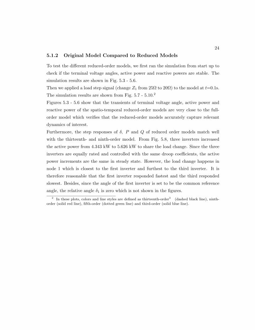
5.3 Terminal voltage angle transients from startup comparing the original
13th-order and the spatio-temporal reduced models: (a)δ2; (b)δ3. . . . . 25
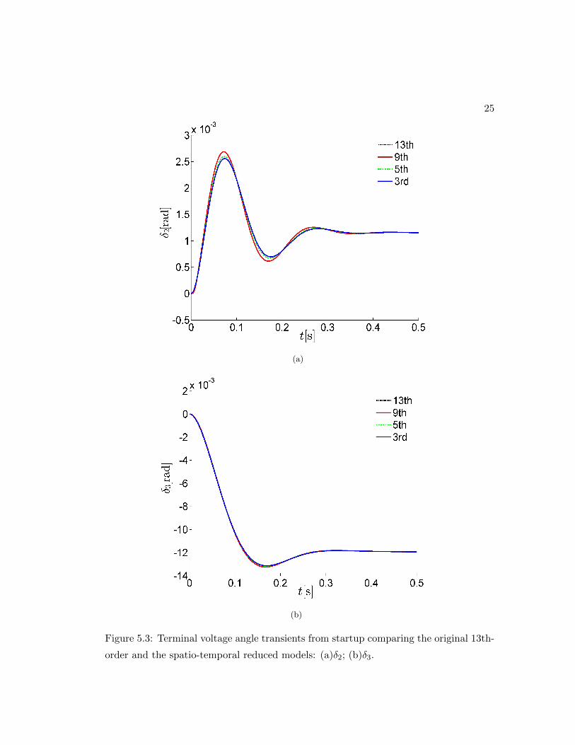
5.4 Active power transients from startup comparing the original 13th-order
and the spatio-temporal reduced models: (a)P1; (b)P2. . . . . . . . . . . 26
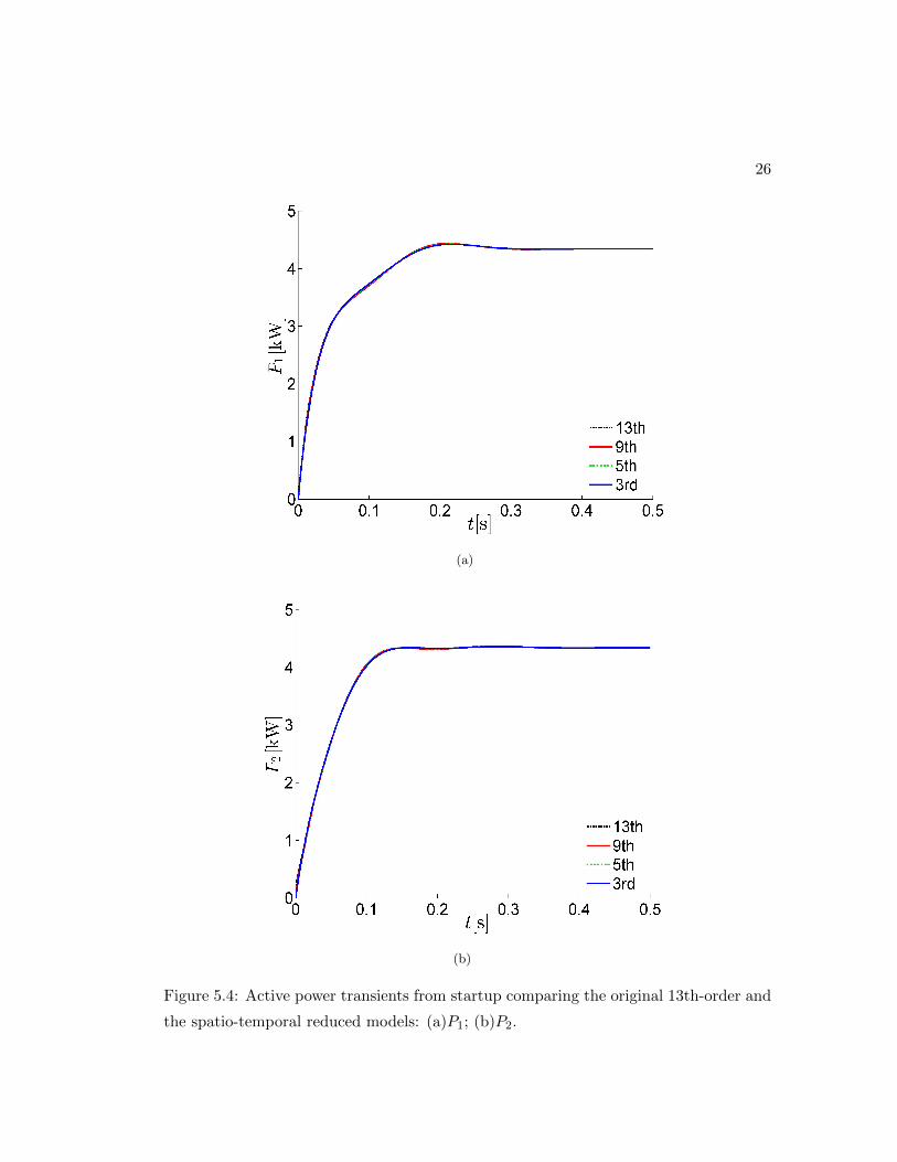
5.5 Active and Reactive power transients from startup comparing the original
13th-order and the spatio-temporal reduced models: (a)P3; (b)Q1. . . . 27
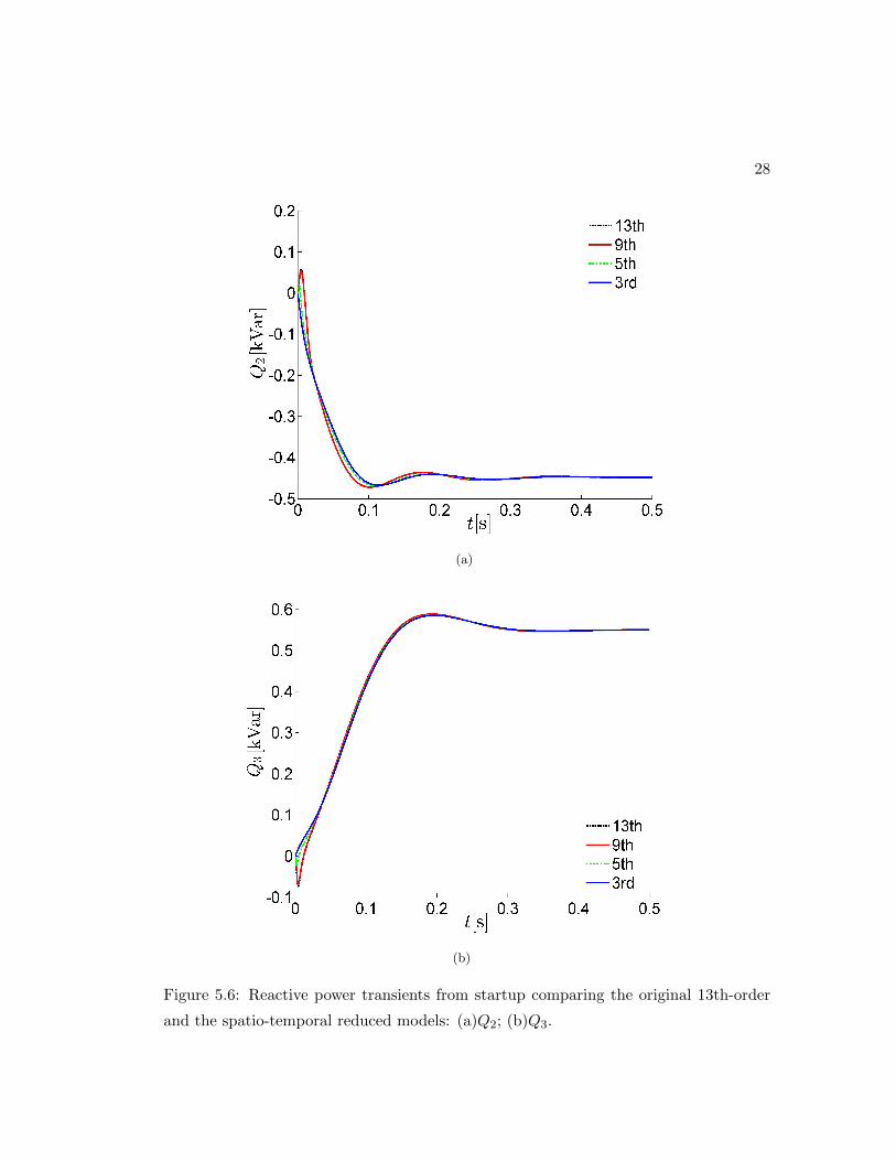
5.6 Reactive power transients from startup comparing the original 13th-order
and the spatio-temporal reduced models: (a)Q2; (b)Q3. . . . . . . . . . 28
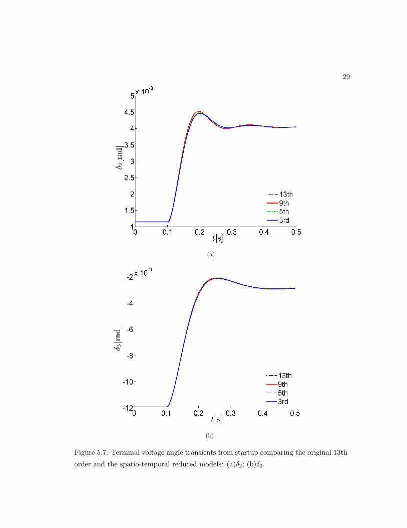
5.7 Terminal voltage angle transients from startup comparing the original
13th-order and the spatio-temporal reduced models: (a)δ2; (b)δ3. . . . . 29
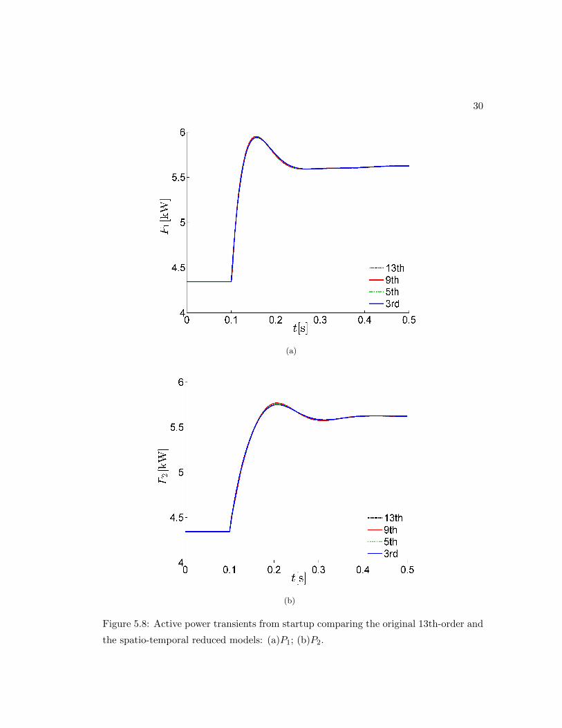
5.8 Active power transients from startup comparing the original 13th-order
and the spatio-temporal reduced models: (a)P1; (b)P2. . . . . . . . . . . 30
vii
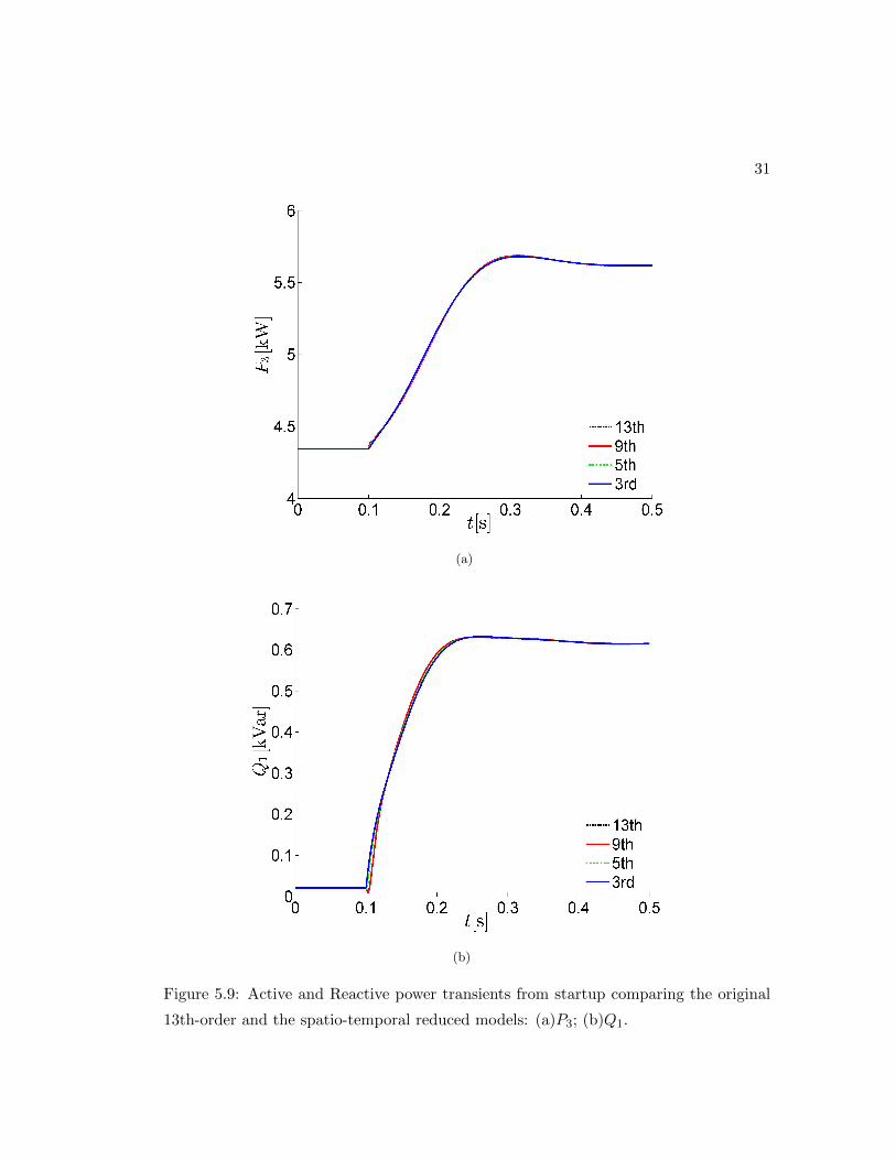
5.9 Active and Reactive power transients from startup comparing the original
13th-order and the spatio-temporal reduced models: (a)P3; (b)Q1. . . . 31
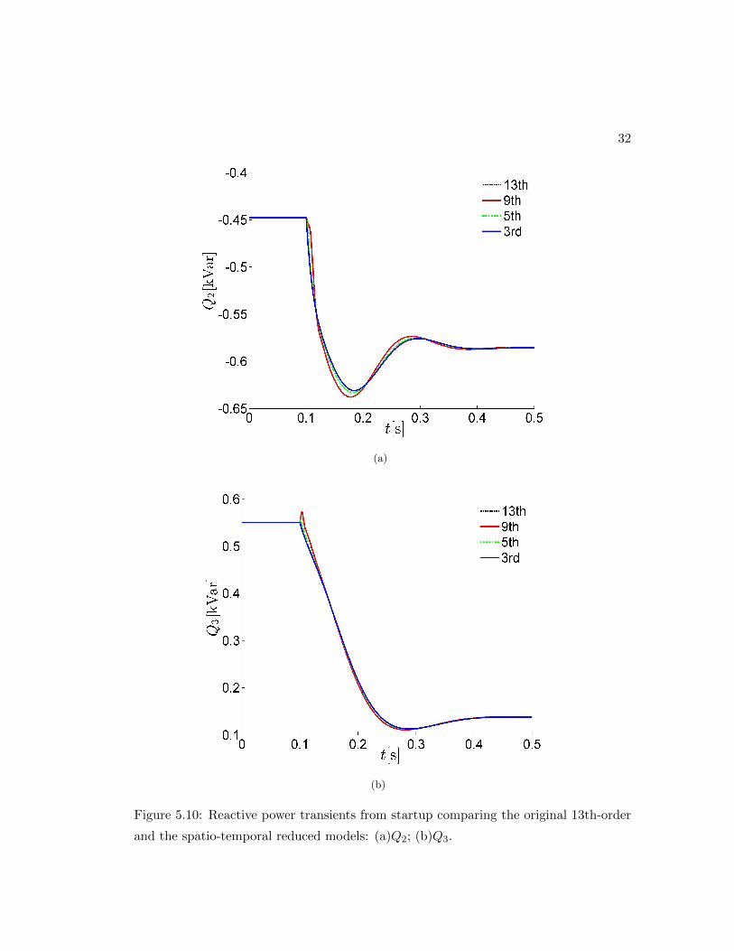
5.10 Reactive power transients from startup comparing the original 13th-order
and the spatio-temporal reduced models: (a)Q2; (b)Q3. . . . . . . . . . 32
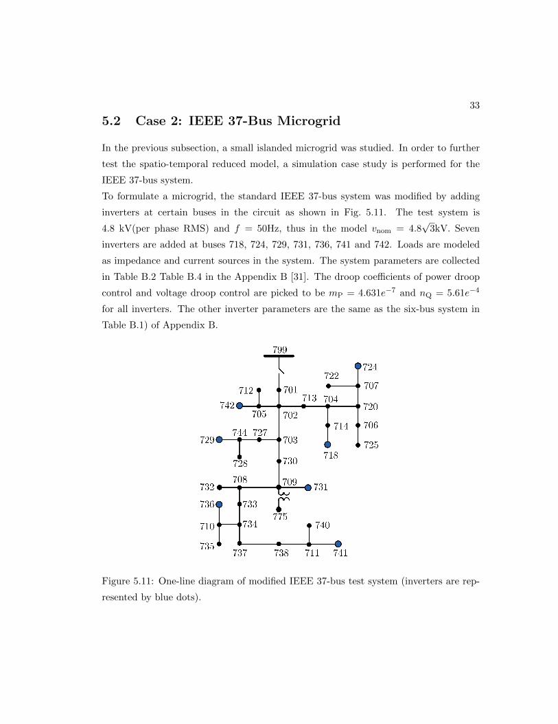
5.11 One-line diagram of modified IEEE 37-bus test system (inverters are
represented by blue dots). . . . . . . . . . . . . . . . . . . . . . . . . . . 33
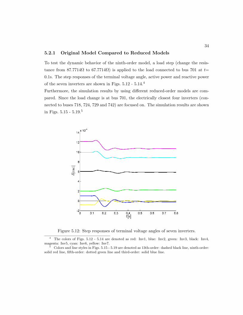
5.12 Step responses of terminal voltage angles of seven inverters. . . . . . . . 34
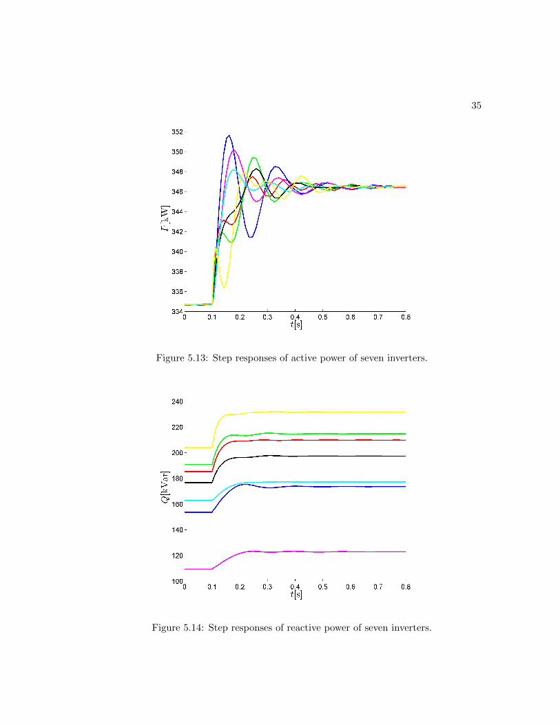
5.13 Step responses of active power of seven inverters. . . . . . . . . . . . . . 35
5.14 Step responses of reactive power of seven inverters. . . . . . . . . . . . . 35
5.15 Step responses of terminal voltage angle comparing the original 13th-order and
the spatio-temporal reduced models: (a)δ2; (b)δ3; (c)δ7 . . . . . . . . . . . . . 36
5.16 Step responses of active power comparing the original 13th-order and the
spatio-temporal reduced models: (a)P1; (b)P2 . . . . . . . . . . . . . . . 37
5.17 Step responses of active power comparing the original 13th-order and the
spatio-temporal reduced models: (a)P3; (b)P7 . . . . . . . . . . . . . . . 38
5.18 Step responses of reactive power comparing the original 13th-order and
the spatio-temporal reduced models: (a)Q1; (b)Q2 . . . . . . . . . . . . 39
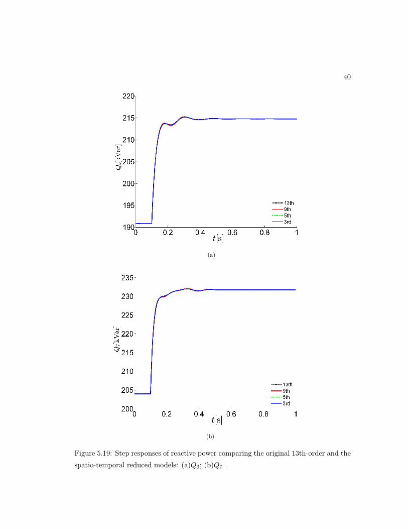
5.19 Step responses of reactive power comparing the original 13th-order and
the spatio-temporal reduced models: (a)Q3; (b)Q7 . . . . . . . . . . . . 40
5.20 Oneline diagram of IEEE 37-bus system after Kron reduction . . . . . . 41
5.21 Scenario 2: step responses of terminal voltage angles of seven inverters. 44
5.22 Scenario 2: step responses of active power of seven inverters. . . . . . . 45
5.23 Scenario 2: step responses of reactive power of seven inverters. . . . . . 45
viii
Chapter 1
Introduction
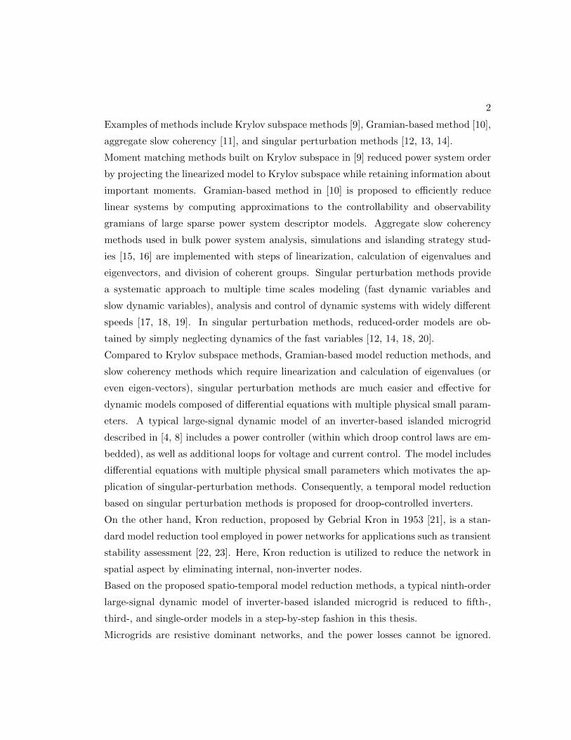
Numerous factors such as energy assurance, reliability, renewable integration, and eco-
nomics are driving increased research and development in the modeling, analysis, and
control of microgrids [1, 2, 3, 4]. To assure the stability and reliability of the micro-
grids, it is important to build dynamical models for microgrids that clearly capture the
interaction of the loads, sources, and power converter circuits.
A microgrid can be operated either in grid-connected mode or islanded mode. In is-
landed operation mode, the microgrid can balance critical loads against available en-
ergy supply while maintaining frequency and voltage within allowed limits by droop
controllers. Droop controllers are designed to mimic the synchronous machines in con-
ventional power system. Typical models for droop-controlled inverters are very detailed,
and include myriad states from internal control loops and filters [4, 5, 6, 7, 8]. Conceiv-
ably, control design, numerical simulations, and stability assessment with such models
in islanded microgrids comprising tens of or even hundreds of inverters is computation-
ally expensive and do not offer any analytical insights. This calls for the development of
model-reduction methods to isolate relevant spatio-temporal dynamics and mutual in-
teractions of interest. While model reduction methods have been widely applied in bulk
power systems, a systematic model-reduction procedure for droop-controlled islanded
inverters has thus far been lacking. To fill the blank, a systematic model reduction
method is proposed in this thesis to reduce large-signal dynamic models of inverter-
based islanded microgrids in both spatial and temporal aspects.
Model reduction techniques for dynamic models of bulk power system are well developed.
1
2
Examples of methods include Krylov subspace methods [9], Gramian-based method [10],
aggregate slow coherency [11], and singular perturbation methods [12, 13, 14].
Moment matching methods built on Krylov subspace in [9] reduced power system order
by projecting the linearized model to Krylov subspace while retaining information about
important moments. Gramian-based method in [10] is proposed to efficiently reduce
linear systems by computing approximations to the controllability and observability
gramians of large sparse power system descriptor models. Aggregate slow coherency
methods used in bulk power system analysis, simulations and islanding strategy stud-
ies [15, 16] are implemented with steps of linearization, calculation of eigenvalues and
eigenvectors, and division of coherent groups. Singular perturbation methods provide
a systematic approach to multiple time scales modeling (fast dynamic variables and
slow dynamic variables), analysis and control of dynamic systems with widely different
speeds [17, 18, 19]. In singular perturbation methods, reduced-order models are ob-
tained by simply neglecting dynamics of the fast variables [12, 14, 18, 20].
Compared to Krylov subspace methods, Gramian-based model reduction methods, and
slow coherency methods which require linearization and calculation of eigenvalues (or
even eigen-vectors), singular perturbation methods are much easier and effective for
dynamic models composed of differential equations with multiple physical small param-
eters. A typical large-signal dynamic model of an inverter-based islanded microgrid
described in [4, 8] includes a power controller (within which droop control laws are em-
bedded), as well as additional loops for voltage and current control. The model includes
differential equations with multiple physical small parameters which motivates the ap-
plication of singular-perturbation methods. Consequently, a temporal model reduction
based on singular perturbation methods is proposed for droop-controlled inverters.
On the other hand, Kron reduction, proposed by Gebrial Kron in 1953 [21], is a stan-
dard model reduction tool employed in power networks for applications such as transient
stability assessment [22, 23]. Here, Kron reduction is utilized to reduce the network in
spatial aspect by eliminating internal, non-inverter nodes.
Based on the proposed spatio-temporal model reduction methods, a typical ninth-order
large-signal dynamic model of inverter-based islanded microgrid is reduced to fifth-,
third-, and single-order models in a step-by-step fashion in this thesis.
Microgrids are resistive dominant networks, and the power losses cannot be ignored.
3
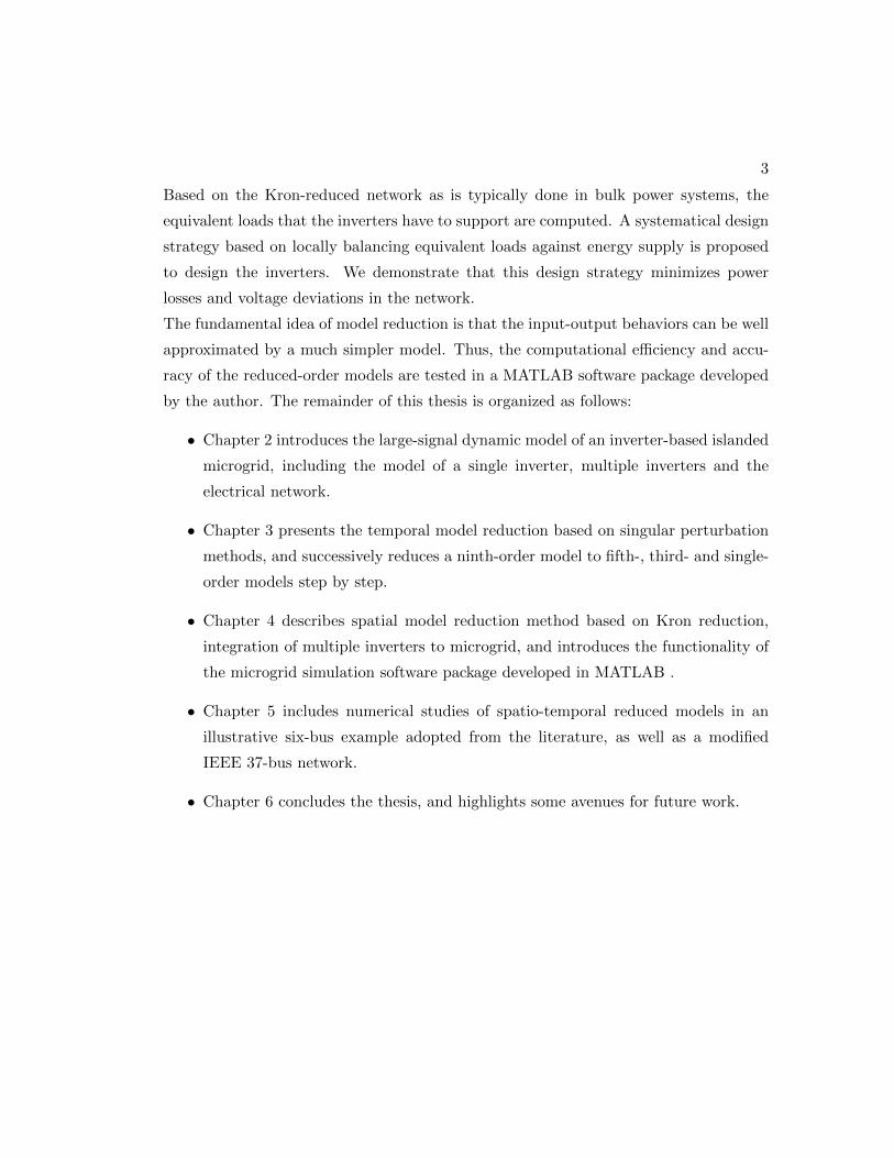
Based on the Kron-reduced network as is typically done in bulk power systems, the
equivalent loads that the inverters have to support are computed. A systematical design
strategy based on locally balancing equivalent loads against energy supply is proposed
to design the inverters. We demonstrate that this design strategy minimizes power
losses and voltage deviations in the network.
The fundamental idea of model reduction is that the input-output behaviors can be well
approximated by a much simpler model. Thus, the computational efficiency and accu-
racy of the reduced-order models are tested in a MATLAB software package developed
by the author. The remainder of this thesis is organized as follows:
• Chapter 2 introduces the large-signal dynamic model of an inverter-based islanded
microgrid, including the model of a single inverter, multiple inverters and the
electrical network.
• Chapter 3 presents the temporal model reduction based on singular perturbation
methods, and successively reduces a ninth-order model to fifth-, third- and single-
order models step by step.
• Chapter 4 describes spatial model reduction method based on Kron reduction,
integration of multiple inverters to microgrid, and introduces the functionality of
the microgrid simulation software package developed in MATLAB .
• Chapter 5 includes numerical studies of spatio-temporal reduced models in an
illustrative six-bus example adopted from the literature, as well as a modified
IEEE 37-bus network.
• Chapter 6 concludes the thesis, and highlights some avenues for future work.
Chapter 2
System Model
In this chapter, the system model of inverter-based islanded microgrids is described.
We start from the model of single droop-controlled inverter, then move on to the model
of microgrids composed of multiple inverters, and finally the network model.
2.1 Single Inverter Model
A microgrid can operate in both grid-connected mode and islanded mode. In case is-
landed operation mode, frequency and voltage are maintained by a primary control strat-
egy based on active power and reactive power droop control [4, 7, 8, 24, 25, 26](usually
embedded in the power controller). In particular, the voltage and frequency of inverters
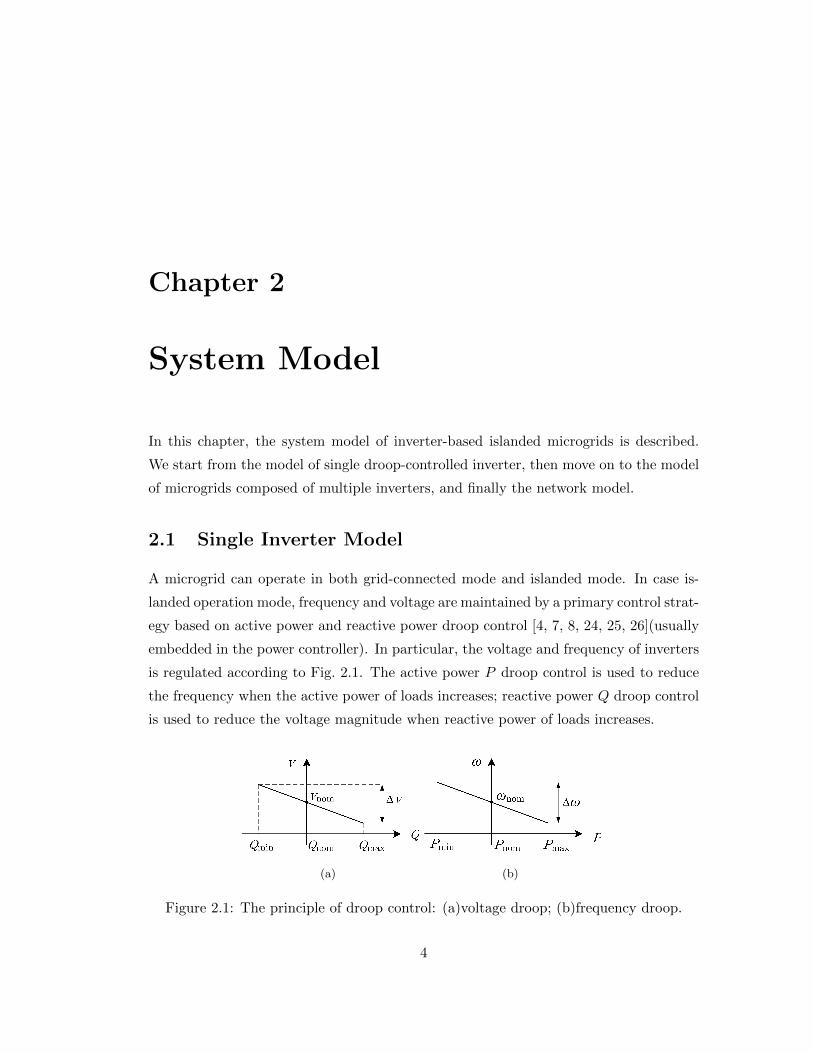
is regulated according to Fig. 2.1. The active power P droop control is used to reduce
the frequency when the active power of loads increases; reactive power Q droop control
is used to reduce the voltage magnitude when reactive power of loads increases.
(a) (b)
Figure 2.1: The principle of droop control: (a)voltage droop; (b)frequency droop.
4
5
In Fig. 2.1, Vnom (ωnom) is the nominal magnitude of the terminal voltage (nominal
inverter frequency) that the controllers try to regulate to, Qnom (Pnom) is the reactive
power (active power) the inverter should output to support nominal terminal voltage
(nominal frequency). ∆V (∆ω) is the limit of voltage deviation (frequency deviation)
controlled by the slope of the droop control. The slopes of the voltage-reactive power
(frequency-active power) are defined as droop coefficients nQ (mP) which are given by
mP =∆ω
Pmax − Pmin, nQ =
∆V
Qmax −Qmin. (2.1)
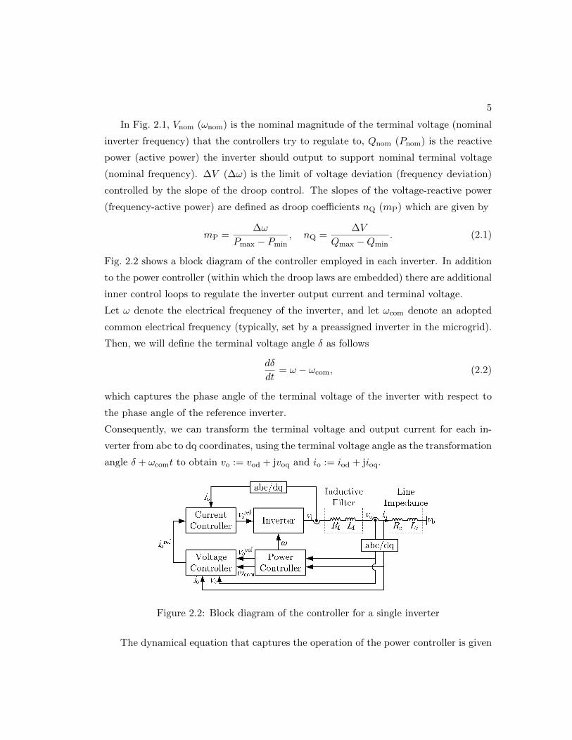
Fig. 2.2 shows a block diagram of the controller employed in each inverter. In addition
to the power controller (within which the droop laws are embedded) there are additional
inner control loops to regulate the inverter output current and terminal voltage.
Let ω denote the electrical frequency of the inverter, and let ωcom denote an adopted
common electrical frequency (typically, set by a preassigned inverter in the microgrid).
Then, we will define the terminal voltage angle δ as follows
dδ
dt= ω − ωcom, (2.2)
which captures the phase angle of the terminal voltage of the inverter with respect to
the phase angle of the reference inverter.
Consequently, we can transform the terminal voltage and output current for each in-
verter from abc to dq coordinates, using the terminal voltage angle as the transformation
angle δ + ωcomt to obtain vo := vod + jvoq and io := iod + jioq.
Figure 2.2: Block diagram of the controller for a single inverter
The dynamical equation that captures the operation of the power controller is given
6
by:1
ωc
dS
dt= −S + voi
∗o, (2.3)
where ωc is the cut-off frequency, and S = P + jQ is the apparent (low-pass filtered)
power delivered by the inverter.1 One output of the power controller is the terminal-
voltage reference
vrefo = vnom − nQS − S∗
2= vnom − nQQ, (2.4)
which captures the voltage-reactive power droop law [4, 27, 24]. The other output, the
inverter frequency, given by
ω = ωnom −mPS + S∗
2= ωnom −mPP, (2.5)
which is governed by the frequency-active power droop law [4, 27, 24].
The voltage- and current-controller state variables are denoted by φ = φd + jφq and
γ = γd + jγq, respectively. Following [4, 5, 8, 28], a conventional PI controller is utilized
to regulate the terminal voltage and output currents to their reference values, denoted
by vrefo and irefo . The voltage- and current-controllers generate the references
irefo = Fio + jω +Kφp
dφ
dt+Kφ
i φ, (2.6)
vrefi = jωnomLf io +Kγp
dγ
dt+Kγ
i γ, (2.7)
where Kφp (Kγ
p ) and Kφi (Kγ
i ) are the proportional (integral) parameters of the voltage
(current) PI control blocks. The controller dynamics are governed by
dφ
dt= vrefo − vo, (2.8)
dγ
dt= irefo − io. (2.9)
Finally, the dynamics of the output current are captured by
Lc
Rc
diodt
= −(
1 + jωLc
Rc
)io +
vo − vbRc
, (2.10)
where vb := vbd + jvbq is the bus voltage at the point of common coupling (PCC).
1 (·)∗ denotes complex conjugation.
7
2.2 Multiple-Inverter Model
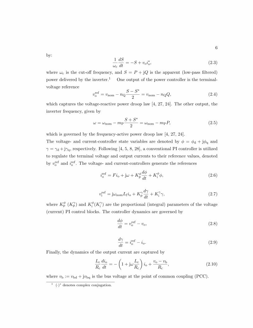
The large-signal dynamic model discussed above is based on individual dq reference
frames for the inverters. In practical microgrids, there are usually more than one in-
verters integrated to the network shown in Fig. 2.3 (a). A common reference frame is
adopted for the whole system, e.g. the reference frame of the first inverter. Letting the
quadrature component of terminal voltage to zero for control purpose, and putting vo
on the direct axis of the corresponding reference frame as shown Fig. 2.3 (b). Denote
the common reference frame as DQ reference frame and the angle of the ith inverter
with respect to the DQ-axis is denoted by δi. Then according to the definition of the
terminal voltage angle in equation (2.2), we get
dδidt
= ωi − ωcom. (2.11)
When integrated to the microgrid through PCC, the voltage and current of the PCC
should be transformed to the common reference frame DQ-axis. Denote vio as the
terminal voltage, and vib as the PCC voltage of the ith inverter. According to Fig. 2.3
(b), the angle of vio with respect to DQ-axis is δi, and the angle of vib is θi + δi.
(a) (b)
Figure 2.3: Multiple inverters integrated to microgrid: (a) block diagram; (b) angle
reference frames.
Consequently, a microgrid which contains N inverters, the coordinate transformation
between the common DQ-axis and the dq-axis for the individual inverters is given by
vDQo = Tvo, (2.12)
8
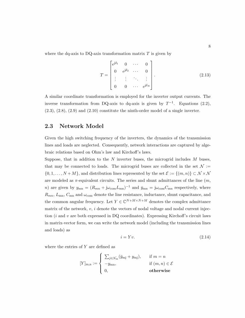
where the dq-axis to DQ-axis transformation matrix T is given by
T =
ejδ1 0 · · · 0
0 ejδ2 · · · 0...
.... . .
...
0 0 · · · ejδN
. (2.13)
A similar coordinate transformation is employed for the inverter output currents. The
inverse transformation from DQ-axis to dq-axis is given by T−1. Equations (2.2),
(2.3), (2.8), (2.9) and (2.10) constitute the ninth-order model of a single inverter.
2.3 Network Model
Given the high switching frequency of the inverters, the dynamics of the transmission
lines and loads are neglected. Consequently, network interactions are captured by alge-
braic relations based on Ohm’s law and Kirchoff’s laws.
Suppose, that in addition to the N inverter buses, the microgrid includes M buses,
that may be connected to loads. The microgrid buses are collected in the set N :=
0, 1, . . . , N +M, and distribution lines represented by the set E := (m,n) ⊂ N ×Nare modeled as π-equivalent circuits. The series and shunt admittances of the line (m,
n) are given by ymn = (Rmn + jωcomLmn)−1 and ymn = jωcomCmn respectively, where
Rmn, Lmn, Cmn and ωcom denote the line resistance, inductance, shunt capacitance, and
the common angular frequency. Let Y ∈ CN+M×N+M denotes the complex admittance
matrix of the network, v, i denote the vectors of nodal voltage and nodal current injec-
tion (i and v are both expressed in DQ coordinates). Expressing Kirchoff’s circuit laws
in matrix-vector form, we can write the network model (including the transmission lines
and loads) as
i = Y v. (2.14)
where the entries of Y are defined as
[Y ]m,n :=
∑
j∈Nm(ymj + ymj), if m = n
−ymn, if (m,n) ∈ E0, otherwise
9
and Nm := j ∈ N : (m, j) ∈ E denotes the set of buses connected to the mth bus
through a distribution line.
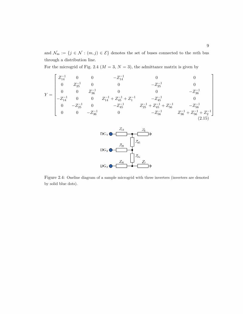
For the microgrid of Fig. 2.4 (M = 3, N = 3), the admittance matrix is given by
Y =
Z−114 0 0 −Z−114 0 0
0 Z−125 0 0 −Z−125 0
0 0 Z−136 0 0 −Z−136
−Z−114 0 0 Z−114 + Z−145 + Z−11 −Z−145 0
0 −Z−125 0 −Z−145 Z−125 + Z−145 + Z−156 −Z−156
0 0 −Z−136 0 −Z−156 Z−136 + Z−156 + Z−12
(2.15)
Figure 2.4: Oneline diagram of a sample microgrid with three inverters (inverters are denoted
by solid blue dots).
Chapter 3
Temporal Model Reduction
In Chapter 2, we discussed a ninth-order large-signal dynamic model of droop-controlled
inverters, which include myriad states from internal control loops and filters [4, 8, 5].
Conceivably, control design, numerical simulations, and stability assessment with such
models in islanded microgrids comprising tens of or even hundreds of inverters is com-
putationally expensive and do not offer any analytical insights.
In this Chapter, we propose a model-reduction method based on singular perturbation
to obtain reduced-order models for individual inverters. Based on the proposed method,
the original ninth-order model includes states of power controller, voltage and current
controllers, and inductive filter (x = [δ, S, φ, γ, io]T), which is suitable for detailed
studies that capture controller dynamics, is reduced to fifth-, third-, and single-order
models.
The reduced order large-signal dynamic models are useful in different contexts. The
fifth-order model only considers the angle, power and current dynamics (x = [δ, S, io]T),
which can be used to analyze output current and power dynamics; the reduced third-
order model (x = [δ, S]T) is sufficiently accurate for dynamic simulation and reliability
assessment of large microgrids, and the single-order model which has a unique state
variable (x = δ) is suitable for design of secondary-level controllers.
10
11
3.1 Temporal Model Reduction Based on Singular Pertur-
bation Methods
For dynamical systems which exhibit different dynamic response speeds, fast dynamic
variables represent the states which respond faster, and slow dynamic variables repre-
sent states that respond slower. The main idea of singular perturbation methods is to
reduce model order by eliminating the fast dynamic state variables. Thus, fast dynamic
variables are assumed to instantaneously reach its quasi-steady-state solution, which
governed by algebraic equations [12, 14, 18, 20, 29].
The dynamic model of a system with multiple time scales can be written in the standard
singular perturbation form [12, 13, 30]
dx
dt= f(x, z, u, t, ε), (3.1)
εdz
dt= g(x, z, u, t, ε), (3.2)
where x ∈ Cn×1, is the vector that collects the slow dynamic variables, z ∈ Cm×1, is the
vector that collects the fast dynamic variables, and u is the input, ε = diag ε1, ε2, · · · , εmdenotes a diagonal matrix with non-zero entries comprised of the small-perturbation pa-
rameters.
From [13, Theorem 11.1], we can reduce the system above to a nth-order model by
setting ε = 0 and obtaining the the quasi-steady-state solution
z = h(x, u, t), (3.3)
Substitute h(x, u, t) in (3.2), we get the reduced-order model
dx
dt= f(x, h(x, u, t), u, t, 0), (3.4)
To accomplish the above steps, we require the Jacobian of g(·), given by
∂g(x, z, u, t, ε)
∂z
∣∣∣∣ε=0
(3.5)
to be nonsingular and have eigenvalues with negative real parts [13, 30].
To apply the temporal model reduction method proposed in Section 3.1, we need to
analyze the different time scales of the droop-controlled inverters. To this end, we will
12
use parameters from [4] as a reference.
First, denote τS, τφ, τγ and τf as the time constants of the power controller, voltage
controller, currrent controller and the inductive filter, respectively. The values of the
time constants are given by
τS =1
ωc=
1
31.41= 3.18× 10⁻²s
τφ =1
Kφi
=1
390= 2.3× 10⁻³s
τγ =1
Kγi
=1
16000= 6.25× 10⁻⁵s
τf =Lf
Rf=
1.35× 10⁻³
0.1= 1.35× 10⁻²s
Notice that the time constants of state variables are quite different from each other,
which indicate that droop-controlled inverters have explicit multiple time scales. The
current controller responds fastest (with time constant of 6.25× 10⁻⁵s) and the voltage
controller dynamics are the second fastest (with time constant of 2.3 × 10⁻³s). The
inductive filter and the power controller react relatively slower (with time constant
about 10−2s).
We pick ε = diag ε1, ε2, ε3, ε4 = diag
1
Kφi
, 1Kγ
i, 1ωc, LfRf
. In the following sections, we
will successively reduce the ninth-order model described in Section 2.1 to a fifth-order
model, a third-order model, and finally a single-order model.
3.2 Reduced Fifth-Order Model
First, we will reduce the ninth-order model to a fifth-order model by eliminating the
dynamical equations for the voltage and current controllers. Notice that the full dynam-
ical model for each inverter, as described by (2.2), (2.3), (2.8), (2.9) and (2.10), includes
nine state variables, δ, P,Q, φd, φq, γd, γq, iod and ioq. For the purpose of analysis, we
will find it useful to write (2.6) and (2.7) in the following form
1
Kφi
dφ
dt= − 1
Kφp
φ− irefo − FioKφ
pKφi
, (3.6)
1
Kγi
dγ
dt= − 1
Kγpγ − vrefi − jωnomLfio
KγpK
γi
, (3.7)
13
We can rewrite the ninth-order model (as described in equations (2.2), (2.3), (2.10),
(3.6) and (3.7)) of a single inverter in the standard singular perturbation form [12, 13,
30].dx
dt= f(x, z, u, t, ε), (3.8)
εdz
dt= g(x, z, u, t, ε). (3.9)
In (3.8) and (3.9), x = [δ, S, io]T ∈ C3×1, is the vector that collects the slow dynamic
variables, z = [φ, γ]T ∈ C2×1, is the vector that collects the fast dynamic variables,
and u = vb is the input (the PCC bus voltage is adopted as the input). In addition,
ε = diag ε1, ε2 = diag
1
Kφi
, 1Kγ
i
denotes a diagonal matrix with non-zero entries
comprised of the small-perturbation parameters. It is easy to show that the vector
fields f(·) and g(·) are given by
f =
ωnom −mP
S+S∗
2 − ωcom
−ωcS + ωcvoi∗o
−(RcLc
+ jω)io + vo−vb
Lc
, (3.10)
g =
− 1
Kφpφ− ε1 i
refo −FioKφ
p
− 1Kγ
pγ − ε2
vrefi −jωnomLf ioKγ
p
, (3.11)
The Jacobian of g(·)
∂g
∂z
∣∣∣∣ε=0
=
− 1
Kφp
0
0 − 1Kγ
p
. (3.12)
Notice that the Jacobian is nonsingular, and has two eigenvalues − 1
Kφp
and − 1Kγ
p, which
have negative real parts. Setting ε = 0 in (3.8) and (3.9) we obtain
dx
dt= f(x, z, u, t, 0), (3.13)
0 = g(x, z, u, t, 0) =
− 1
Kφpφ
− 1Kγ
pγ
. (3.14)
14
Solving (3.14), we obtain the quasi-steady-state solution for z which is given by
z = h(x, u, t) =
[0
0
]. (3.15)
This implies dφdt = 0 and dγ
dt = 0. From (2.8) and (2.9), we conclude
vrefo = vo, irefo = io. (3.16)
Substituting the solution of z in (3.13), we can obtain the following reduced fifth-order
model of a single droop-controlled inverter:
dx
dt= f(x, h(x, u, t), u, t, 0) =
ωnom −mP
S+S∗
2 − ωcom
−ωcS + ωcvrefo i∗o
−(RcLc
+ jω)io + vrefo −u
Lc
, (3.17)
where x = [δ, S, io]T ∈ C3×1 is the vector that collects the slow dynamic variables and
u = vb. Notice that we have neglected the dynamic of the fast dynamic variables in the
description above.
It is easy to interpret the reduced model of inverter by reviewing the block diagram
of a single inverter as shown in Fig. 2.2. From a high-level view, the model reduction
procedure eliminated the dynamics of the voltage controller and current controller.
In conclusion, (3.17) describes the fifth-order model where only the angle, power and
filter current dynamics are retained. The complete model of the fifth-order model is
described in Appendix A Section A.3.
3.3 Reduced Third-Order Model
We can further reduce the fifth-order model concluded in Section 3.2 to a third-order
and a single-order model step by step. The reduced fifth-order model of (3.17) can be
rewritten in the standard singular perturbation form as
dx
dt= f(x, z, u, t, ε), (3.18)
εdz
dt= g(x, z, u, t, ε), (3.19)
15
In (3.18) and (3.19), x = [δ, S]T ∈ C2×1, is the vector that collects the slow dynamic
variables, z = io ∈ C1×1, is the complex variable which captures the dynamics of the
output current (fast dynamic variable), and u = vb is the input (the PCC bus voltage
is adopted as the input). In addition, ε = ε3 = LcRc
. It is easy to show that the vector
fields f(·) and g(·) are given by
f =
[ωnom −mP
S+S∗
2 − ωcom
−ωcS + ωcvrefo i∗o
], (3.20)
g = − (1 + jωε3) io +vrefo − uRc
, (3.21)
Similarly to the previous section, first, we calculate the gradient of g(·) which is −1 in
this case. It is easy to verify that the gradient satisfies the requirements of singular
perturbation model reduction. Then, we set ε3 = 0 in (3.19) to obtain
z = h(x, u, t) = io =vrefo − uRc
. (3.22)
Substituting io in (3.18), and we can obtain the reduced third-order model of a single
inverter as follows
dx
dt= f(x, h(x, u, t), u, t, 0) =
[ωnom −mP
S+S∗
2 − ωcom
−ωcS + ωcvrefo (v
refo −uRc
)∗
], (3.23)
Notice that the quasi-steady-state solution of the fast dynamic variable io = vrefo −uRc
can
be derived by applying Ohm’s law to the physical output R-L filter circuit and neglecting
the line inductance. The complete set of equations that describe the third-order model
are given in Appendix A Section A.2.
3.4 Reduced Single-Order Model
Finally, we reduce the third-order model to a single-order model. At this point, the
reduced third-order model of Equation (3.23) can be rewritten in the usual standard
singular perturbation form as
dx
dt= f(x, z, u, t, ε), (3.24)
16
εdz
dt= g(x, z, u, t, ε), (3.25)
In (3.24) and (3.25), x = δ is the variable that collects the slow dynamic variable
(terminal voltage angle), z = S is the complex variable which captures the fast dynamic
variables (low-pass filtered apparent power), and u = vb is the input. In addition,
ε = ε4 = 1ωc
. It is easy to show that f(·) and g(·) are given by
f = ωnom −mPS + S∗
2− ωcom, (3.26)
g = −S + vrefo i∗o, (3.27)
As before, first we calculate the gradient of g(·) which is −1 in this case. It is easy
to verify that the gradient satisfies the requirements of singular perturbation model
reduction. Then, we set ε4 = 0 in (3.25) and obtain
S = vrefo i∗o = vrefo (vrefo − uRc
)∗. (3.28)
Substituting S in (3.24), we can conclude that the reduced single-order model of a single
inverter is given by
dδ
dt= ωnom −mP
S + S∗
2− ωcom, (3.29)
S = vrefo i∗o = vrefo
(vrefo − uRc
)∗. (3.30)
It follows that the quasi-steady-state solution of the fast dynamic variable in the reduced
third-order model S = vrefo i∗o is the definition of the apparent power when neglecting
the dynamics of the power controller.
In this Chapter, we reduced the large-signal dynamic model of a single inverter from
the ninth-order to a single-order model step by step based on singular perturbation
methods. In the next Chapter, the spatial model reduction of the network based on
Kron reduction will be presented. The complete models of the different order models
are given in Appendix A.
Chapter 4
Spatial Model Reduction
Kron reduction is a standard tool employed in power networks for applications such
as transient stability assessment [21, 22]. Here, Kron reduction is utilized to eliminate
internal, non-inverter nodes, and isolate the mutual inverter interactions. This allows
us to significantly increase simulation efficiency, and provides more insight into the mi-
crogrid dynamics [22].
4.1 Kron Reduction
Suppose, that in addition to the N inverter nodes, the microgrid includes M nodes,
that may be connected to loads. Let Y ∈ CN+M×N+M denotes the complex admittance
matrix of the network, i denote the vector of nodal current injections, and let v denote
the vector of nodal voltages (i and v are both expressed inDQ coordinates corresponding
to the reference inverter). Expressing Kirchoff’s circuit laws in matrix-vector form, we
can write
i = Y v. (4.1)
Let vα ∈ CN×1 (vβ ∈ CM×1) denote the vector of voltages of the nodes connected
(not connected, respectively) to inverters, and let iα ∈ CN×1 (iβ ∈ CM×1) denote the
vector of current injections at the nodes connected (not connected, respectively) to the
17
18
inverters. Then (4.1) can be expressed as[iα
iβ
]=
[Yαα Yαβ
Y Tαβ Yββ
][vα
vβ
]. (4.2)
Since the loads in the microgrid are constant impedances or currents, Kron reduction
allows us to eliminate vβ, to obtain
iα = (Yαα − YαβY −1ββ YTαβ)vα + YαβY
−1ββ iβ = YKronvα + YαβY
−1ββ iβ. (4.3)
Basically, (4.3) means the inverter current injections are related to terminal voltages
through the admittance matrix of Kron-reduced network (YKron = Yαα − YαβY −1ββ YTαβ),
and the current loads are mapped to individual inverters through YαβY−1ββ . Furthermore,
the absence of vβ implies that only the mutual inverter interactions between inverters
are retained. And, YKron captures equivalent local loads and equivalent series impedance
that link inverters.
4.2 Input of Inverter Dynamical Models
Assume there are N inverter nodes and M non-inverter nodes in the microgrid. Without
loss of generality, assume the first N nodes are connected with inverters while others
may be connected to loads. For simplicity of discussion, here we assume there are only
impedance loads in the network, then equation (4.1) will be
iα = Ykrvα = (Yαα − YαβY −1ββ YTαβ)vα. (4.4)
In the dynamic simulation of microgrids, we need to solve two parts (the differential-
algebraic model for the inverters, and the algebraic equations of the network) separately
within one iteration. First we solve for bus voltage 1
vα = Y −1Kroniα (4.5)
where
iα = Tio, vα = Tvb. (4.6)
1 Generally, the equivalent loads of shunt impedance connected to inverter buses are non-zero, YKron
is invertible.
19
Then, we transform the PCC bus voltage from DQ-axis to the dq-axis for individual
inverters by vib = e−jδiviα. Written in matrix form, the input of the inverter differential
equations is given by
u = vb = T−1Y −1kr Tio. (4.7)
where the dq-axis to DQ-axis transformation matrix T is defined in equation (2.13).
Then, set vb as the input of the differential equations of the inverters and solve the state
variables (shown in Chapter 3).
4.3 Software Package Developed in MATLAB
In Chapters 3 and 4, we obtained reduced-order models of droop-controlled islanded in-
verters. To test the spatio-temporal reduced order models, a software package including
the original thirteenth-order model from [4, 8], the ninth-order and the reduced fifth-
and third-order models are implemented in MATLAB.2
The developed software package can create selected order of large-signal dynamic model
of inverter-based islanded microgrid with any number of inverters. To make the numer-
ical study results comparable, the same MATLAB functions are used to solve the DAE
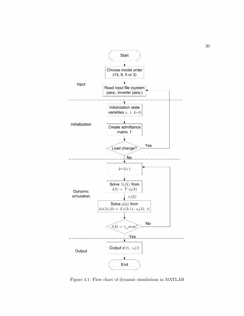
equations. The flow chart of coding the dynamical system model of different orders (13,
9, 5, 3) in MATLAB is shown in Figure 4.1. The software package in MATLAB consists
four functionality blocks:
(1) Input block: read in inverter data, network parameters and load steps information.
(2) Admittance matrix block: which creates Y matrix, and implements Kron reduction
(obtains YKron) for impedance loads and current loads.
(3) Inverter model block: create selected order large-signal dynamic model of microgrids
based on input data and calculated admittance matrix.
(4) Output block: output the chosen simulation results, including state variables, power
losses, maximum voltage deviations, dq components and abc components of output cur-
rents and terminal voltages.
2 A coupling capacitor paralleled to the inductive filter in thirteenth-order model is neglected inthe ninth-order model, because the capacitor is really small and it has high natural frequency which ismuch faster than the dynamics of other electrical variables, such as inductor current, terminal voltageand apparent power.
20
Figure 4.1: Flow chart of dynamic simulations in MATLAB
Chapter 5
Numerical Studies
Based on the MATLAB software package discussed in Section 4.3, two numerical cases
are studied in this Chapter. Case 1 is a six-bus microgrid with three inverters and
designed at 220V (per-phase RMS); Case 2 is a modified IEEE 37-bus system with seven
inverters and designed at 4.8kV (per-phase RMS). Simulation results and analysis are
as follows.
5.1 Case 1: Six-Bus Microgrid
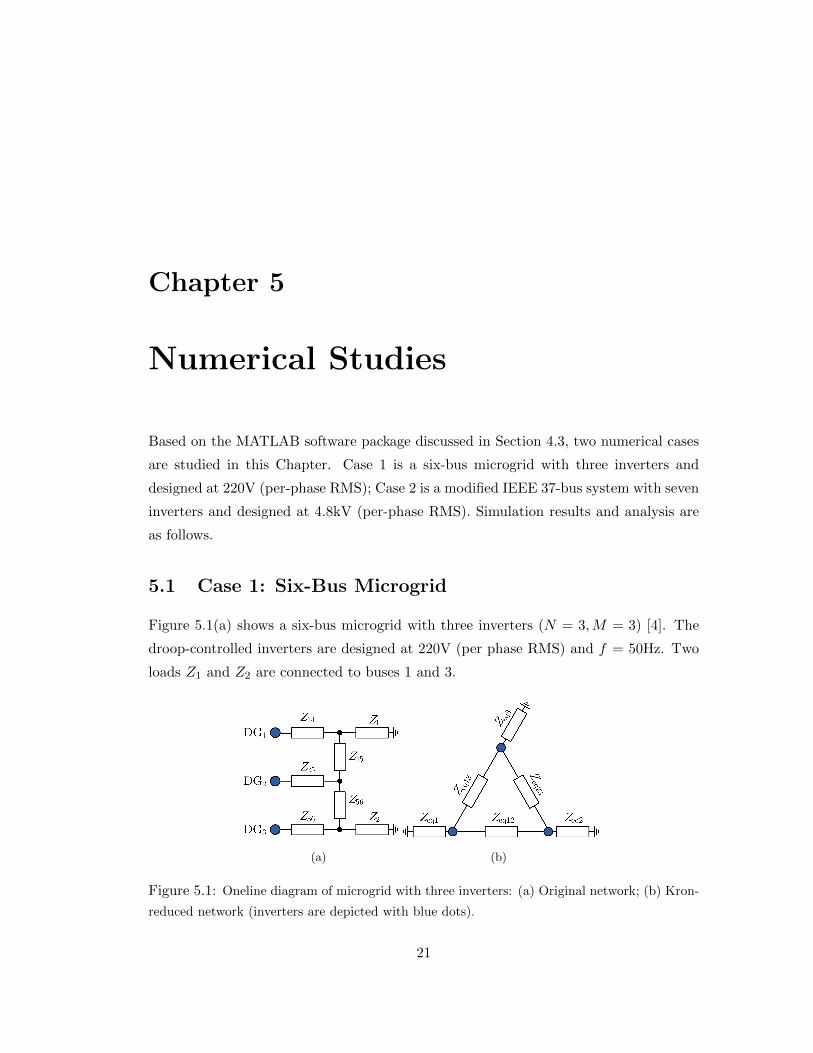
Figure 5.1(a) shows a six-bus microgrid with three inverters (N = 3,M = 3) [4]. The
droop-controlled inverters are designed at 220V (per phase RMS) and f = 50Hz. Two
loads Z1 and Z2 are connected to buses 1 and 3.
(a) (b)
Figure 5.1: Oneline diagram of microgrid with three inverters: (a) Original network; (b) Kron-
reduced network (inverters are depicted with blue dots).
21
22
Assume that the three inverters are equally rated. Thus, we use the same droop
coefficients for the frequency and voltage controllers. Furthermore, for the initial stud-
ies, we assume the loads are resistive with per-phase parameters listed in Table 5.1,
and current loads are disregarded (iβ = 0). The Kron-reduced network is shown in
Figure 5.1(b).
Table 5.1: Network parameters of Case 1
Parameter Value(Ω) Parameter Value(Ω)
Z14 0.03 +j0.11 Z25 0.03 +j0.11
Z36 0.03 +j0.11 Z45 0.23 +j0.1
Z56 0.35+j0.58 Z1 25
Z2 20
For this Kron-reduced network, we will compare the different reduced-order models
described next.
5.1.1 Responses of Fast and Slow Dynamic Variables
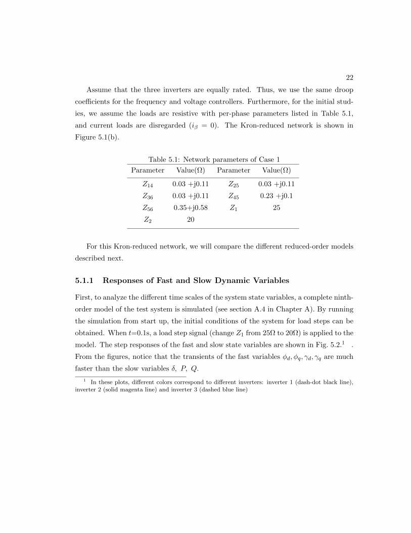
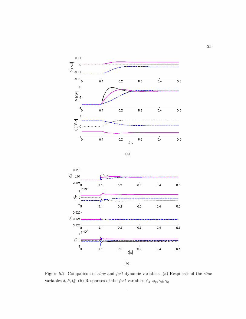
First, to analyze the different time scales of the system state variables, a complete ninth-
order model of the test system is simulated (see section A.4 in Chapter A). By running
the simulation from start up, the initial conditions of the system for load steps can be
obtained. When t=0.1s, a load step signal (change Z1 from 25Ω to 20Ω) is applied to the
model. The step responses of the fast and slow state variables are shown in Fig. 5.2.1 .
From the figures, notice that the transients of the fast variables φd, φq, γd, γq are much
faster than the slow variables δ, P, Q.
1 In these plots, different colors correspond to different inverters: inverter 1 (dash-dot black line),inverter 2 (solid magenta line) and inverter 3 (dashed blue line)
23
(a)
(b)
Figure 5.2: Comparison of slow and fast dynamic variables. (a) Responses of the slow
variables δ, P,Q; (b) Responses of the fast variables φd, φq, γd, γq
.
24
5.1.2 Original Model Compared to Reduced Models
To test the different reduced-order models, we first ran the simulation from start up to
check if the terminal voltage angles, active power and reactive powers are stable. The
simulation results are shown in Fig. 5.3 - 5.6.
Then we applied a load step signal (change Z1 from 25Ω to 20Ω) to the model at t=0.1s.
The simulation results are shown from Fig. 5.7 - 5.10.2
Figures 5.3 - 5.6 show that the transients of terminal voltage angle, active power and
reactive power of the spatio-temporal reduced-order models are very close to the full-
order model which verifies that the reduced-order models accurately capture relevant
dynamics of interest.
Furthermore, the step responses of δ, P and Q of reduced order models match well
with the thirteenth- and ninth-order model. From Fig. 5.8, three inverters increased
the active power from 4.343 kW to 5.626 kW to share the load change. Since the three
inverters are equally rated and controlled with the same droop coefficients, the active
power increments are the same in steady state. However, the load change happens in
node 1 which is closest to the first inverter and furthest to the third inverter. It is
therefore reasonable that the first inverter responded fastest and the third responded
slowest. Besides, since the angle of the first inverter is set to be the common reference
angle, the relative angle δ1 is zero which is not shown in the figures.
2 In these plots, colors and line styles are defined as thirteenth-order3 (dashed black line), ninth-order (solid red line), fifth-order (dotted green line) and third-order (solid blue line).
25
(a)
(b)
Figure 5.3: Terminal voltage angle transients from startup comparing the original 13th-
order and the spatio-temporal reduced models: (a)δ2; (b)δ3.
26
(a)
(b)
Figure 5.4: Active power transients from startup comparing the original 13th-order and
the spatio-temporal reduced models: (a)P1; (b)P2.
27
(a)
(b)
Figure 5.5: Active and Reactive power transients from startup comparing the original
13th-order and the spatio-temporal reduced models: (a)P3; (b)Q1.
28
(a)
(b)
Figure 5.6: Reactive power transients from startup comparing the original 13th-order
and the spatio-temporal reduced models: (a)Q2; (b)Q3.
29
(a)
(b)
Figure 5.7: Terminal voltage angle transients from startup comparing the original 13th-
order and the spatio-temporal reduced models: (a)δ2; (b)δ3.
30
(a)
(b)
Figure 5.8: Active power transients from startup comparing the original 13th-order and
the spatio-temporal reduced models: (a)P1; (b)P2.
31
(a)
(b)
Figure 5.9: Active and Reactive power transients from startup comparing the original
13th-order and the spatio-temporal reduced models: (a)P3; (b)Q1.
32
(a)
(b)
Figure 5.10: Reactive power transients from startup comparing the original 13th-order
and the spatio-temporal reduced models: (a)Q2; (b)Q3.
33
5.2 Case 2: IEEE 37-Bus Microgrid
In the previous subsection, a small islanded microgrid was studied. In order to further
test the spatio-temporal reduced model, a simulation case study is performed for the
IEEE 37-bus system.
To formulate a microgrid, the standard IEEE 37-bus system was modified by adding
inverters at certain buses in the circuit as shown in Fig. 5.11. The test system is
4.8 kV(per phase RMS) and f = 50Hz, thus in the model vnom = 4.8√
3kV. Seven
inverters are added at buses 718, 724, 729, 731, 736, 741 and 742. Loads are modeled
as impedance and current sources in the system. The system parameters are collected
in Table B.2 Table B.4 in the Appendix B [31]. The droop coefficients of power droop
control and voltage droop control are picked to be mP = 4.631e−7 and nQ = 5.61e−4
for all inverters. The other inverter parameters are the same as the six-bus system in
Table B.1) of Appendix B.
Figure 5.11: One-line diagram of modified IEEE 37-bus test system (inverters are rep-
resented by blue dots).
34
5.2.1 Original Model Compared to Reduced Models
To test the dynamic behavior of the ninth-order model, a load step (change the resis-
tance from 87.7714Ω to 67.7714Ω) is applied to the load connected to bus 701 at t=
0.1s. The step responses of the terminal voltage angle, active power and reactive power
of the seven inverters are shown in Figs. 5.12 - 5.14.4
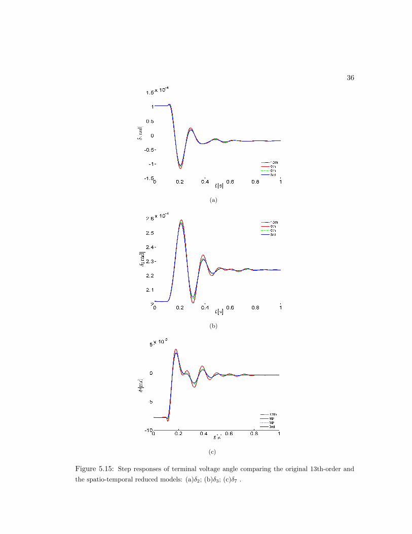
Furthermore, the simulation results by using different reduced-order models are com-
pared. Since the load change is at bus 701, the electrically closest four inverters (con-
nected to buses 718, 724, 729 and 742) are focused on. The simulation results are shown
in Figs. 5.15 - 5.19.5
Figure 5.12: Step responses of terminal voltage angles of seven inverters.
4 The colors of Figs. 5.12 - 5.14 are denoted as red: Inv1, blue: Inv2, green: Inv3, black: Inv4,magenta: Inv5, cyan: Inv6, yellow: Inv7.
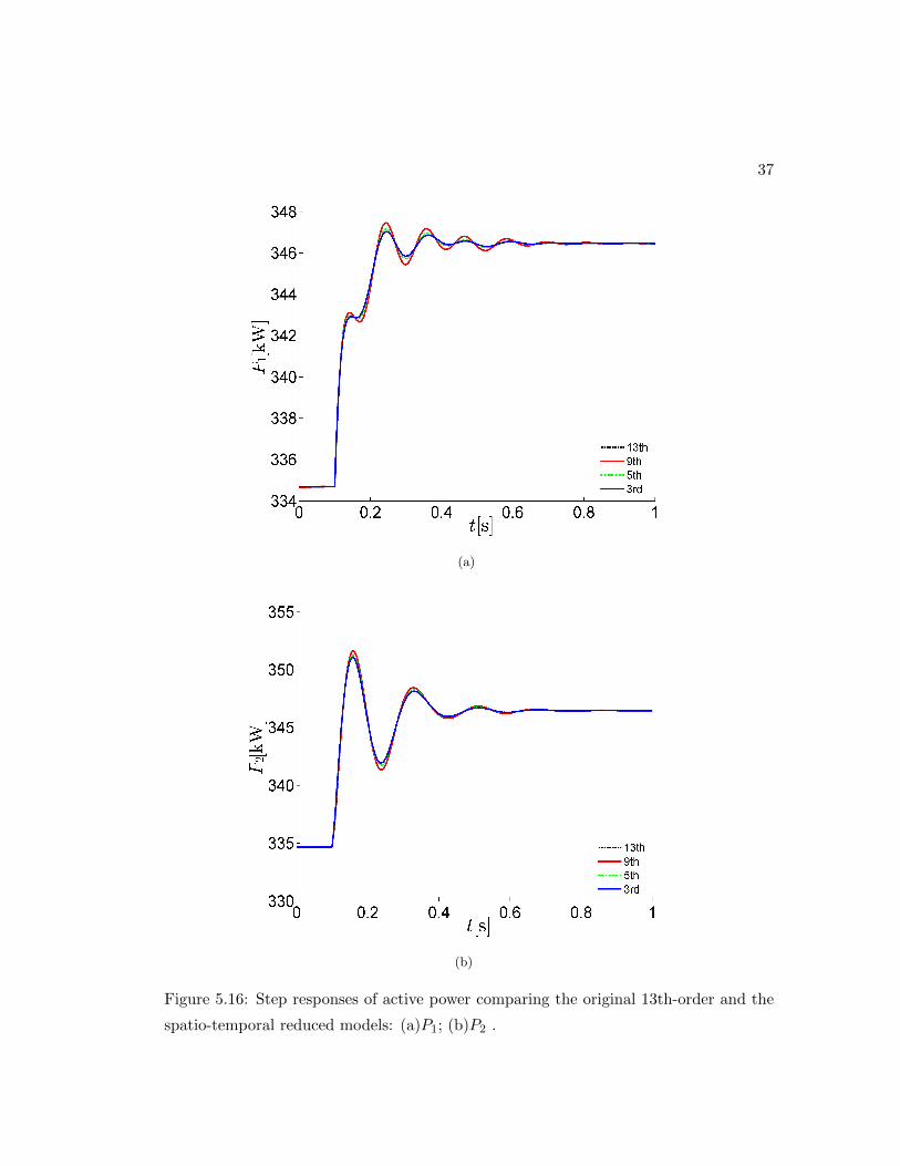
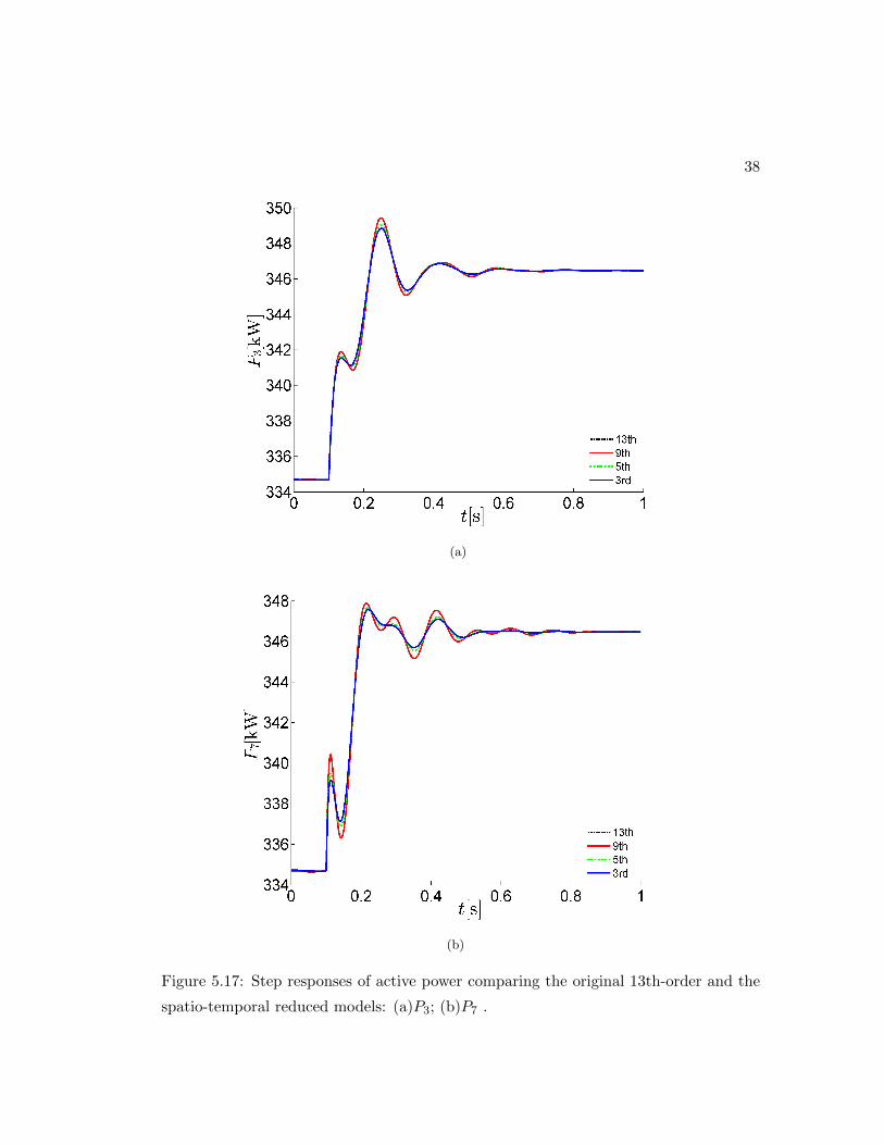
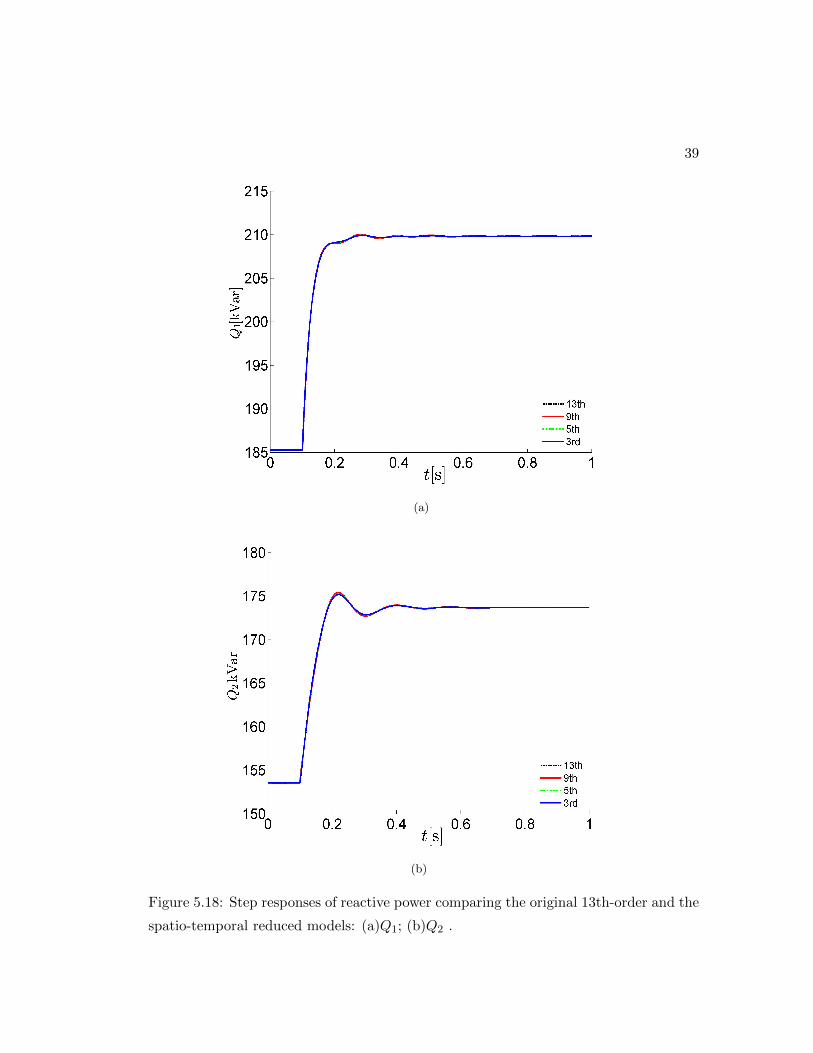
5 Colors and line styles in Figs. 5.15 - 5.19 are denoted as 13th-order: dashed black line, ninth-order:solid red line, fifth-order: dotted green line and third-order: solid blue line.
35
Figure 5.13: Step responses of active power of seven inverters.
Figure 5.14: Step responses of reactive power of seven inverters.
36
(a)
(b)
(c)
Figure 5.15: Step responses of terminal voltage angle comparing the original 13th-order and
the spatio-temporal reduced models: (a)δ2; (b)δ3; (c)δ7 .
37
(a)
(b)
Figure 5.16: Step responses of active power comparing the original 13th-order and the
spatio-temporal reduced models: (a)P1; (b)P2 .
38
(a)
(b)
Figure 5.17: Step responses of active power comparing the original 13th-order and the
spatio-temporal reduced models: (a)P3; (b)P7 .
39
(a)
(b)
Figure 5.18: Step responses of reactive power comparing the original 13th-order and the
spatio-temporal reduced models: (a)Q1; (b)Q2 .
40
(a)
(b)
Figure 5.19: Step responses of reactive power comparing the original 13th-order and the
spatio-temporal reduced models: (a)Q3; (b)Q7 .
41
5.2.2 Systematic Design of Droop Coefficients
In most of the studied droop-controlled inverters, equally rated inverters with the same
droop coefficients were employed [4, 7]. However, loads are practically distributed un-
equally. In this case, equivalent loads cannot be balanced by the electrical closest sources
which means power flows through between inverters. And this causes power losses and
voltage deviations. When locally balanced loads against supplies, the power flow be-
tween inverters will be minimized which reducing the power losses and voltage deviations
significantly. Thus, we propose an systematical droop coefficients design method based
on Kron-reduced network to minimize power losses and voltage deviations.
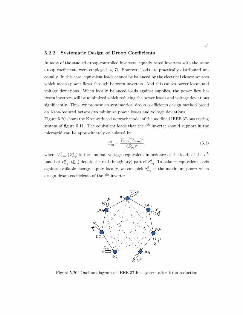
Figure 5.20 shows the Kron-reduced network model of the modified IEEE 37-bus testing
system of figure 5.11. The equivalent loads that the ith inverter should support in the
microgrid can be approximately calculated by
Sieq =Vnom(Vnom)∗
(Zieq)∗, (5.1)
where V inom (Zieq) is the nominal voltage (equivalent impedance of the load) of the ith
bus. Let P ieq (Qieq) denote the real (imaginary) part of Sieq. To balance equivalent loads
against available energy supply locally, we can pick Sieq as the maximum power when
design droop coefficients of the ith inverter.
Figure 5.20: Oneline diagram of IEEE 37-bus system after Kron reduction
42
Furthermore, to mimic the dynamic behavior of synchronous machines, all units in
service should adjust their active power outputs to achieve the same frequency incre-
ments (or decrements) when loads decrease (or increase). Assuming: (1) the nominal
frequency and magnitude of terminal voltage of all inverters are the same; (2) minimum
active (reactive) power Pmin (Qmin) are zeros, and picking 0.05% (2%) as frequency
(voltage) deviation limits in droop controls, then from (2.1) we have
miP =
0.05%ωnom
P imax
, niQ =2%VnomQimax
. (5.2)
When load changes, we denote ∆Pi (∆ωi) as active power (frequency) variation of the
ith inverter. From (2.5), we have
ωi + ∆ωi = ωnom −miP(P i + ∆P i), (5.3)
In (5.2), (5.3) and notice that ωi = ωnom −miPP
i, we obtain
∆ωi = −miP∆P i = −0.05%ωnom
P imax
∆P i. (5.4)
From (5.4), ∆P i is proportional to its maximum capacity P imax in steady state when
frequency deviation of all inverters are the same. A similar analysis can be employed
for voltage deviation and maximum reactive power.
Based on the equivalent loads obtained from Kron reduction in (5.1) and the conclusion
that ∆P i is proportional to P imax in steady state, we let
P imax = P ieq, (5.5)
Qimax = Qieq. (5.6)
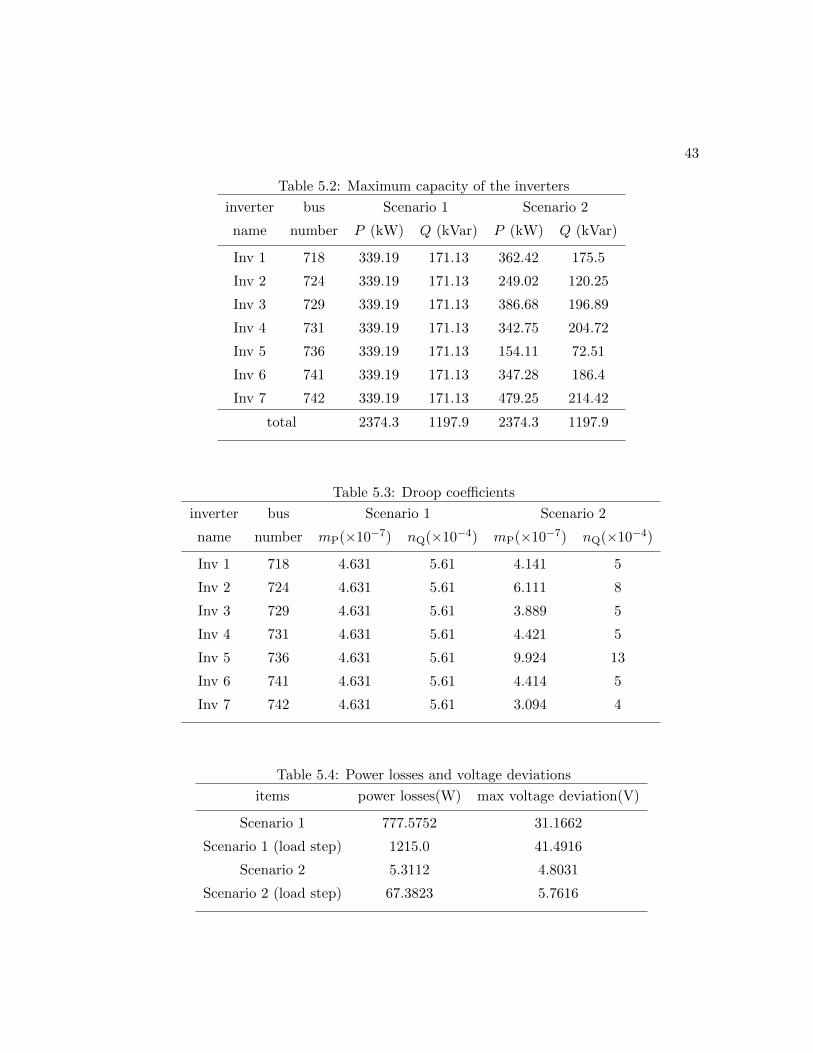
and design droop coefficients by (5.2). To verify the systematically designed droop
coefficients, we build two scenarios for microgrid shown in Fig. 5.11. The equivalent
loads and droop coefficients of the two scenarios are listed in Table 5.2 and 5.3. Notice
that scenario 1 has been discussed in Subsection 5.2.1.
43
Table 5.2: Maximum capacity of the inverters
inverter bus Scenario 1 Scenario 2
name number P (kW) Q (kVar) P (kW) Q (kVar)
Inv 1 718 339.19 171.13 362.42 175.5
Inv 2 724 339.19 171.13 249.02 120.25
Inv 3 729 339.19 171.13 386.68 196.89
Inv 4 731 339.19 171.13 342.75 204.72
Inv 5 736 339.19 171.13 154.11 72.51
Inv 6 741 339.19 171.13 347.28 186.4
Inv 7 742 339.19 171.13 479.25 214.42
total 2374.3 1197.9 2374.3 1197.9
Table 5.3: Droop coefficients
inverter bus Scenario 1 Scenario 2
name number mP(×10−7) nQ(×10−4) mP(×10−7) nQ(×10−4)
Inv 1 718 4.631 5.61 4.141 5
Inv 2 724 4.631 5.61 6.111 8
Inv 3 729 4.631 5.61 3.889 5
Inv 4 731 4.631 5.61 4.421 5
Inv 5 736 4.631 5.61 9.924 13
Inv 6 741 4.631 5.61 4.414 5
Inv 7 742 4.631 5.61 3.094 4
Table 5.4: Power losses and voltage deviations
items power losses(W) max voltage deviation(V)
Scenario 1 777.5752 31.1662
Scenario 1 (load step) 1215.0 41.4916
Scenario 2 5.3112 4.8031
Scenario 2 (load step) 67.3823 5.7616
44
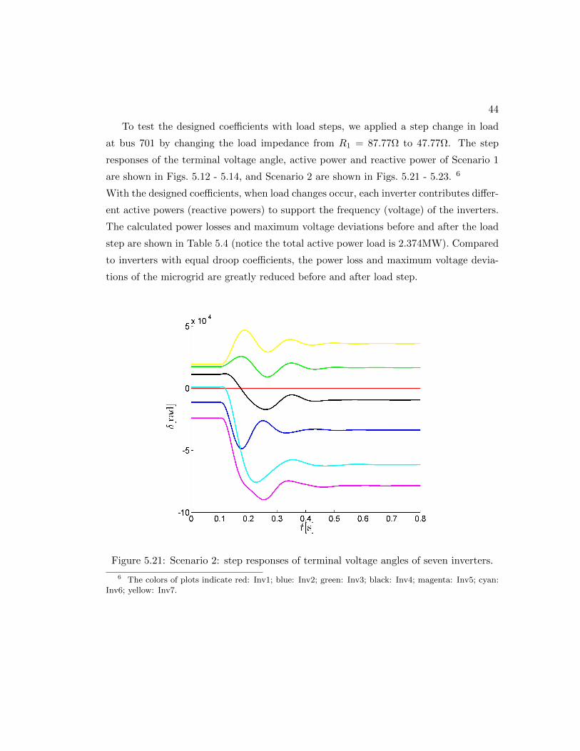
To test the designed coefficients with load steps, we applied a step change in load
at bus 701 by changing the load impedance from R1 = 87.77Ω to 47.77Ω. The step
responses of the terminal voltage angle, active power and reactive power of Scenario 1
are shown in Figs. 5.12 - 5.14, and Scenario 2 are shown in Figs. 5.21 - 5.23. 6
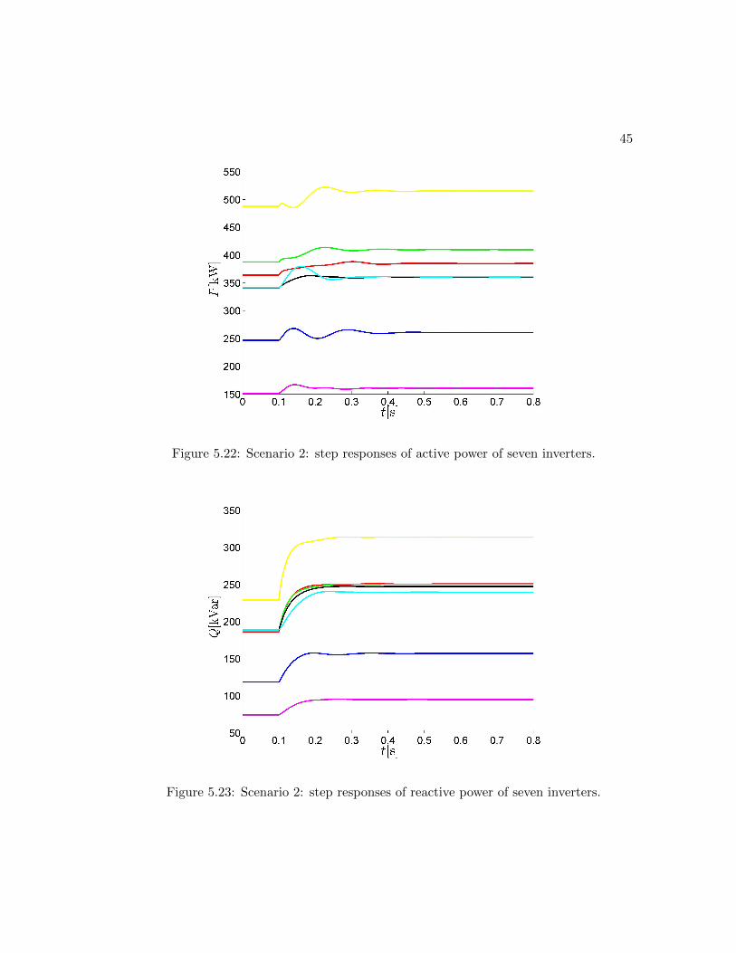
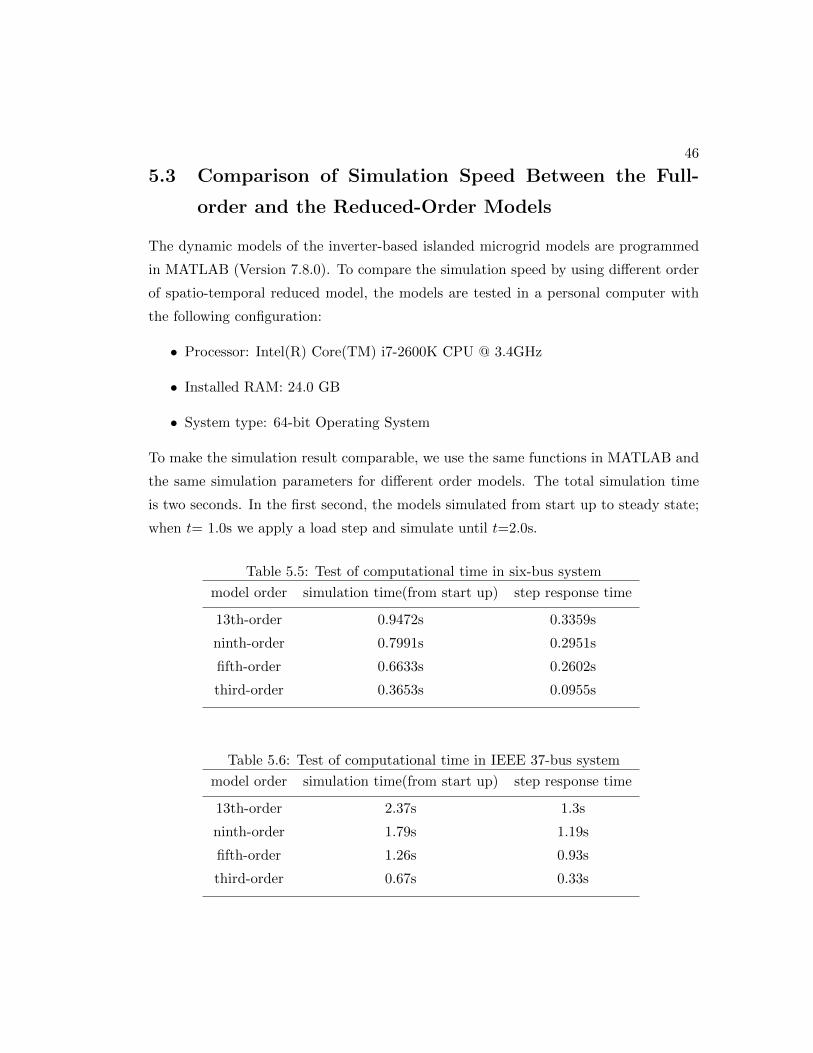
With the designed coefficients, when load changes occur, each inverter contributes differ-
ent active powers (reactive powers) to support the frequency (voltage) of the inverters.
The calculated power losses and maximum voltage deviations before and after the load
step are shown in Table 5.4 (notice the total active power load is 2.374MW). Compared
to inverters with equal droop coefficients, the power loss and maximum voltage devia-
tions of the microgrid are greatly reduced before and after load step.
Figure 5.21: Scenario 2: step responses of terminal voltage angles of seven inverters.
6 The colors of plots indicate red: Inv1; blue: Inv2; green: Inv3; black: Inv4; magenta: Inv5; cyan:Inv6; yellow: Inv7.
45
Figure 5.22: Scenario 2: step responses of active power of seven inverters.
Figure 5.23: Scenario 2: step responses of reactive power of seven inverters.
46
5.3 Comparison of Simulation Speed Between the Full-
order and the Reduced-Order Models
The dynamic models of the inverter-based islanded microgrid models are programmed
in MATLAB (Version 7.8.0). To compare the simulation speed by using different order
of spatio-temporal reduced model, the models are tested in a personal computer with
the following configuration:
• Processor: Intel(R) Core(TM) i7-2600K CPU @ 3.4GHz
• Installed RAM: 24.0 GB
• System type: 64-bit Operating System
To make the simulation result comparable, we use the same functions in MATLAB and
the same simulation parameters for different order models. The total simulation time
is two seconds. In the first second, the models simulated from start up to steady state;
when t= 1.0s we apply a load step and simulate until t=2.0s.
Table 5.5: Test of computational time in six-bus system
model order simulation time(from start up) step response time
13th-order 0.9472s 0.3359s
ninth-order 0.7991s 0.2951s
fifth-order 0.6633s 0.2602s
third-order 0.3653s 0.0955s
Table 5.6: Test of computational time in IEEE 37-bus system
model order simulation time(from start up) step response time
13th-order 2.37s 1.3s
ninth-order 1.79s 1.19s
fifth-order 1.26s 0.93s
third-order 0.67s 0.33s
47
Tables 5.5 and 5.6 show that compared to the thirteenth-order model [4], the spatio-
temporal reduced third-order model can reduce the simulation time to approximately
one fourth for the modified IEEE 37-bus system, and reduced to approximately one third
compared to the ninth-order reduced model. In conclusion, the spatio-temporal reduced-
order models of the inverter-based islanded microgrids derived in previous chapters are
verified by the simulations to be
• accurately capture relevant dynamic behaviors of the original full-order model;
• can significantly reduce the computational time in the six-bus microgrid and IEEE
37-bus system;
• provide a systematical droop coefficients design strategy that minimizes power
losses and voltage deviations in steady state.
Chapter 6
Conclusions and Future Work
6.1 Conclusions
In this thesis, model reduction methods are proposed for systematically reducing large-
signal dynamic models of inverter-based islanded microgrids in both spatial and tem-
poral aspects. The reduced-order models are verified by numerical simulations to accu-
rately describe the original dynamics of the system with significantly reduced computa-
tional burden. In addition, spatial model reduction method based on Kron reduction is
employed to isolate the mutual inverter interactions and clearly illustrate the equivalent
loads that the inverters have to support in the microgrid. Based on the Kron-reduced
network model, a systematical droop coefficients design strategy is proposed to mini-
mize the power losses and voltage deviations.
One contribution of the thesis is the derivation of the spatio-temporal reduced fifth-
, third- and single-order models from the original large-signal dynamic model of the
inverter-based islanded microgrid, and the development of software package in MAT-
LAB for dynamic simulation of microgrids with different order of inverter models and
any number of buses. The other contribution is the proposed control design strategy
which provides a reference for choosing droop coefficients to minimize power losses and
voltage deviations in steady state.
48

49
6.2 Future Work
The models proposed in this work are expected to aid future efforts in modeling, analysis,
and control of microgrids. In particular, the following awareness of future work are
envisioned:
• In this thesis, only impedance loads and current loads were studied. Constant
power loads could be modeled in this framework.
• We mainly focus on modeling islanded microgrids. Grid connected operation
should be investigated as well.
• Design of sparse control architectures for secondary-level control.
References
[1] Michael Burr, Michael Zimmer, Brian Meloy, James Bertrand, Walter Levesque,
Guy Warner, and John McDonald. Minnesota microgrids: barriers, opportunities,
and pathways toward energy assurance. Technical report, Minnesota Department
of Commerce, 09 2013.
[2] P. Basak, A. K. Saha, S. Chowdhury, and S. P. Chowdhury. Microgrid: Control
techniques and modeling. In Universities Power Engineering Conference (UPEC),
2009 Proceedings of the 44th International, pages 1–5, 2009.
[3] M. Strelec, K. Macek, and A. Abate. Modeling and simulation of a microgrid as a
stochastic hybrid system. In Innovative Smart Grid Technologies (ISGT Europe),
2012 3rd IEEE PES International Conference and Exhibition on, pages 1–9, 2012.
[4] N. Pogaku, M. Prodanovic, and T.C. Green. Modeling, analysis and testing of
autonomous operation of an inverter-based microgrid. Power Electronics, IEEE
Transactions on, 22(2):613 –625, march 2007.
[5] G. S. Ladde, D.D.Ladde D. D. Siljak, G.S., and D D DLadde. Multiparameter
singular perturbations of linear systems with multiple time scales. Automatica,
19(4):385–394, 1983.
[6] Sungwoo Bae and A. Kwasinski. Dynamic modeling and operation strategy for a
microgrid with wind and photovoltaic resources. Smart Grid, IEEE Transactions
on, 3(4):1867 –1876, dec. 2012.
[7] A. Bidram and A. Davoudi. Hierarchical structure of microgrids control system.
Smart Grid, IEEE Transactions on, 3(4):1963–1976, 2012.
50
51
[8] A. Bidram, A. Davoudi, F.L. Lewis, and J.M. Guerrero. Distributed cooperative
secondary control of microgrids using feedback linearization. Power Systems, IEEE
Transactions on, PP(99):1–9, 2013.
[9] D. Chaniotis and M. A. Pai. Model reduction in power systems using krylov sub-
space methods. Power Systems, IEEE Transactions on, 20(2):888–894, 2005.
[10] F.D. Freitas, J. Rommes, and N. Martins. Gramian-based reduction method applied
to large sparse power system descriptor models. Power Systems, IEEE Transactions
on, 23(3):1258–1270, 2008.
[11] J.H. Chow, R. Galarza, P. Accari, and W.W. Price. Inertial and slow coherency
aggregation algorithms for power system dynamic model reduction. Power Systems,
IEEE Transactions on, 10(2):680–685, 1995.
[12] E.H. Abed and R. Silva-Madriz. Stability of systems with multiple very small and
very large parasitics. Circuits and Systems, IEEE Transactions on, 34(9):1107–
1110, 1987.
[13] H. Khalil. Nonlinear Systems. Prentice Hall, Upper Saddle River, NJ, 2002.
[14] H. Khalil. Stability analysis of nonlinear multiparameter singularly perturbed sys-
tems. Automatic Control, IEEE Transactions on, 32(3):260–263, 1987.
[15] Guangyue Xu and V. Vittal. Slow coherency based cutset determination algorithm
for large power systems. Power Systems, IEEE Transactions on, 25(2):877–884,
2010.
[16] Guangyue Xu, V. Vittal, A. Meklin, and J.E. Thalman. Controlled islanding
demonstrations on the wecc system. Power Systems, IEEE Transactions on,
26(1):334–343, 2011.
[17] Jr. P. V. Kokotovic, R. E. O’Malley and P. Sannuti. Singular perturbations and
order reduction in control theory–an overview. Automatica, 12:123–132, 1976.
[18] H. K. Khalil. Asymptotic stability of nonlinear multiparameter singularly per-
turbed systems. Automatica, 17(1):797–804, 1978.
52
[19] X. Xu, R. M. Mathur, J. Jiang, G.J. Rogers, and P. Kundur. Modeling of generators
and their controls in power system simulations using singular perturbations. Power
Systems, IEEE Transactions on, 13(1):109–114, 1998.
[20] J. H. Chow. Asymptotic stability of a class of nonlinear singularity perturbed
systems. J. Franklin Inst., 305:123–132, 1978.
[21] Gabriel Kron. A method to solve very large physical systems in easy stages. Circuit
Theory, Transactions of the IRE Professional Group on, PGCT-2:71–90, 1953.
[22] F. Dorfler and F. Bullo. Kron reduction of graphs with applications to electri-
cal networks. Circuits and Systems I: Regular Papers, IEEE Transactions on,
60(1):150–163, 2013.
[23] R.M. Ciric, Antonio Padilha Feltrin, and L.F. Ochoa. Power flow in four-wire
distribution networks-general approach. Power Systems, IEEE Transactions on,
18(4):1283–1290, 2003.
[24] J.M. Guerrero, J.C. Vasquez, J. Matas, L.G. de Vicuna, and M. Castilla. Hi-
erarchical control of droop-controlled ac and dc microgrids - a general approach
toward standardization. Industrial Electronics, IEEE Transactions on, 58(1):158–
172, 2011.
[25] R. Majumder, B. Chaudhuri, A. Ghosh, R. Majumder, G. Ledwich, and F. Zare.
Improvement of stability and load sharing in an autonomous microgrid using sup-
plementary droop control loop. Power Systems, IEEE Transactions on, 25(2):796–
808, 2010.
[26] T.L. Vandoorn, B. Meersman, J.D.M. De Kooning, and L. Vandevelde. Transi-
tion from islanded to grid-connected mode of microgrids with voltage-based droop
control. Power Systems, IEEE Transactions on, 28(3):2545–2553, 2013.
[27] Qing-Chang Zhong. Robust droop controller for accurate proportional load sharing
among inverters operated in parallel. Industrial Electronics, IEEE Transactions on,
60(4):1281–1290, 2013.
53
[28] Y.A. Mohamed and A.A. Radwan. Hierarchical control system for robust microgrid
operation and seamless mode transfer in active distribution systems. Smart Grid,
IEEE Transactions on, 2(2):352 –362, june 2011.
[29] H. Khalil. Stability analysis of nonlinear multiparameter singularly perturbed sys-
tems. In American Control Conference, 1987, pages 1219–1223, 1987.
[30] D. Peponides, P. V. Kokotovic, and J. H. Chow. Singular perturbations and time
scales in nonlinear models of power system. Circuits and Systems, IEEE Transac-
tions on, 29(11):758–767, 1982.
[31] Shengyi Su. Integrated feeder switching and voltage control for increasing dis-
tributed generation penetration. Master’s thesis, National Sun Yat-Sen University,
2009.
Appendix A
Detailed Models
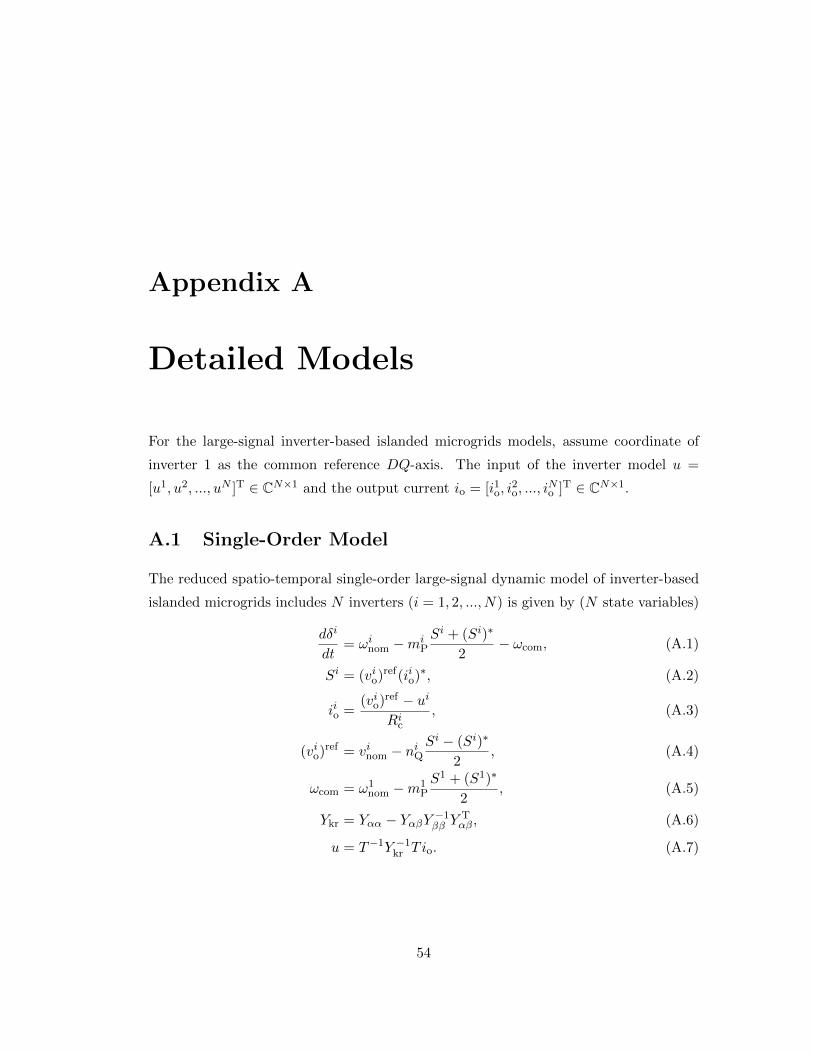
For the large-signal inverter-based islanded microgrids models, assume coordinate of
inverter 1 as the common reference DQ-axis. The input of the inverter model u =
[u1, u2, ..., uN ]T ∈ CN×1 and the output current io = [i1o, i2o, ..., i
No ]T ∈ CN×1.
A.1 Single-Order Model
The reduced spatio-temporal single-order large-signal dynamic model of inverter-based
islanded microgrids includes N inverters (i = 1, 2, ..., N) is given by (N state variables)
dδi
dt= ωinom −mi
P
Si + (Si)∗
2− ωcom, (A.1)
Si = (vio)ref(iio)
∗, (A.2)
iio =(vio)
ref − ui
Ric, (A.3)
(vio)ref = vinom − niQ
Si − (Si)∗
2, (A.4)
ωcom = ω1nom −m1
P
S1 + (S1)∗
2, (A.5)
Ykr = Yαα − YαβY −1ββ YTαβ, (A.6)
u = T−1Y −1kr Tio. (A.7)
54
55
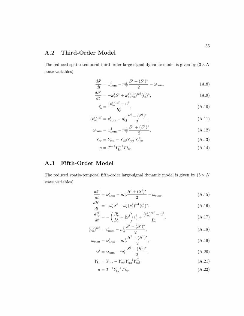
A.2 Third-Order Model
The reduced spatio-temporal third-order large-signal dynamic model is given by (3×Nstate variables)
dδi
dt= ωinom −mi
P
Si + (Si)∗
2− ωcom, (A.8)
dSi
dt= −ωicSi + ωic(v
io)
ref(iio)∗, (A.9)
iio =(vio)
ref − ui
Ric, (A.10)
(vio)ref = vinom − niQ
Si − (Si)∗
2, (A.11)
ωcom = ω1nom −m1
P
S1 + (S1)∗
2, (A.12)
Ykr = Yαα − YαβY −1ββ YTαβ, (A.13)
u = T−1Y −1kr Tio. (A.14)
A.3 Fifth-Order Model
The reduced spatio-temporal fifth-order large-signal dynamic model is given by (5×Nstate variables)
dδi
dt= ωinom −mi
P
Si + (Si)∗
2− ωcom, (A.15)
dSi
dt= −ωicSi + ωic(v
io)
ref(iio)∗, (A.16)
diiodt
= −(RicLic
+ jωi)iio +
(vio)ref − ui
Lic, (A.17)
(vio)ref = vinom − niQ
Si − (Si)∗
2, (A.18)
ωcom = ω1nom −m1
P
S1 + (S1)∗
2, (A.19)
ωi = ωcom −miP
Si + (S1)∗
2, (A.20)
Ykr = Yαα − YαβY −1ββ YTαβ, (A.21)
u = T−1Y −1kr Tio. (A.22)
56
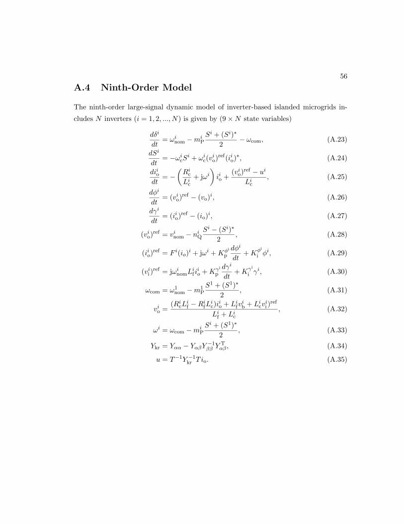
A.4 Ninth-Order Model
The ninth-order large-signal dynamic model of inverter-based islanded microgrids in-
cludes N inverters (i = 1, 2, ..., N) is given by (9×N state variables)
dδi
dt= ωinom −mi
P
Si + (Si)∗
2− ωcom, (A.23)
dSi
dt= −ωicSi + ωic(v
io)
ref(iio)∗, (A.24)
diiodt
= −(RicLic
+ jωi)iio +
(vio)ref − ui
Lic, (A.25)
dφi
dt= (vio)
ref − (vo)i, (A.26)
dγi
dt= (iio)
ref − (io)i, (A.27)
(vio)ref = vinom − niQ
Si − (Si)∗
2, (A.28)
(iio)ref = F i(io)
i + jωi +Kφi
p
dφi
dt+Kφi
i φi, (A.29)
(vii )ref = jωinomL
ifiio +Kγi
p
dγi
dt+Kγi
i γi, (A.30)
ωcom = ω1nom −m1
P
S1 + (S1)∗
2, (A.31)
vio =(RicL
if −RifLic)iio + Lifv
ib + Licv
ii )
ref
Lif + Lic, (A.32)
ωi = ωcom −miP
Si + (S1)∗
2, (A.33)
Ykr = Yαα − YαβY −1ββ YTαβ, (A.34)
u = T−1Y −1kr Tio. (A.35)
Appendix B
Simulation Parameters
B.1 Six-Bus System
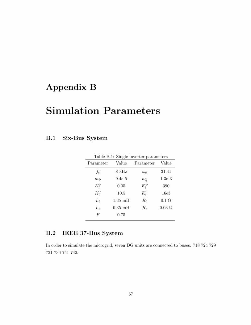
Table B.1: Single inverter parameters
Parameter Value Parameter Value
fs 8 kHz ωc 31.41
mP 9.4e-5 nQ 1.3e-3
Kφp 0.05 Kφ
i 390
Kγp 10.5 Kγ
i 16e3
Lf 1.35 mH Rf 0.1 Ω
Lc 0.35 mH Rc 0.03 Ω
F 0.75
B.2 IEEE 37-Bus System
In order to simulate the microgrid, seven DG units are connected to buses: 718 724 729
731 736 741 742.
57
58
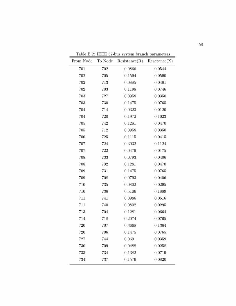
Table B.2: IEEE 37-bus system branch parameters
From Node To Node Resistance(R) Reactance(X)
701 702 0.0866 0.0544
702 705 0.1594 0.0590
702 713 0.0885 0.0461
702 703 0.1198 0.0746
703 727 0.0958 0.0350
703 730 0.1475 0.0765
704 714 0.0323 0.0120
704 720 0.1972 0.1023
705 742 0.1281 0.0470
705 712 0.0958 0.0350
706 725 0.1115 0.0415
707 724 0.3032 0.1124
707 722 0.0479 0.0175
708 733 0.0793 0.0406
708 732 0.1281 0.0470
709 731 0.1475 0.0765
709 708 0.0793 0.0406
710 735 0.0802 0.0295
710 736 0.5106 0.1889
711 741 0.0986 0.0516
711 740 0.0802 0.0295
713 704 0.1281 0.0664
714 718 0.2074 0.0765
720 707 0.3668 0.1364
720 706 0.1475 0.0765
727 744 0.0691 0.0359
730 709 0.0488 0.0258
733 734 0.1382 0.0719
734 737 0.1576 0.0820
59
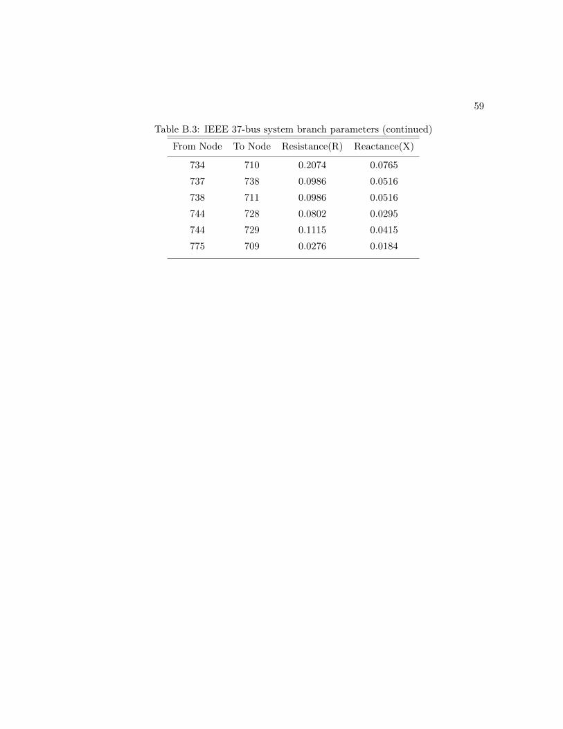
Table B.3: IEEE 37-bus system branch parameters (continued)
From Node To Node Resistance(R) Reactance(X)
734 710 0.2074 0.0765
737 738 0.0986 0.0516
738 711 0.0986 0.0516
744 728 0.0802 0.0295
744 729 0.1115 0.0415
775 709 0.0276 0.0184
60
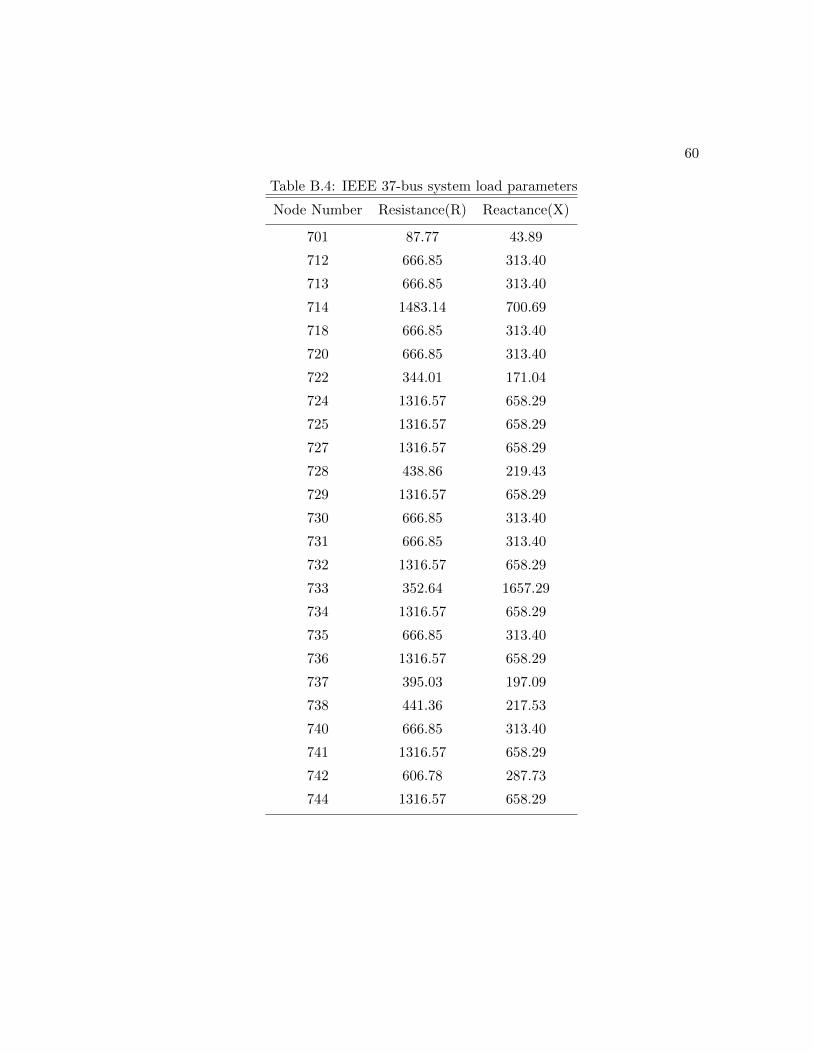
Table B.4: IEEE 37-bus system load parameters
Node Number Resistance(R) Reactance(X)
701 87.77 43.89
712 666.85 313.40
713 666.85 313.40
714 1483.14 700.69
718 666.85 313.40
720 666.85 313.40
722 344.01 171.04
724 1316.57 658.29
725 1316.57 658.29
727 1316.57 658.29
728 438.86 219.43
729 1316.57 658.29
730 666.85 313.40
731 666.85 313.40
732 1316.57 658.29
733 352.64 1657.29
734 1316.57 658.29
735 666.85 313.40
736 1316.57 658.29
737 395.03 197.09
738 441.36 217.53
740 666.85 313.40
741 1316.57 658.29
742 606.78 287.73
744 1316.57 658.29