Embed Size (px)
Citation preview
Thesis for doctoral degree (Ph.D.)
YAMINA SEAMARI
UNIVERSIDAD DE MÁLAGA
FACULTAD DE MEDICINA
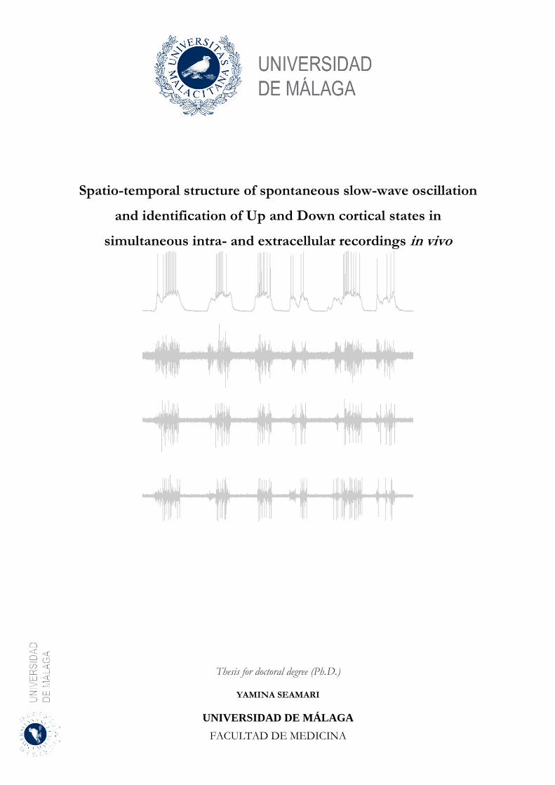
Spatio-temporal structure of spontaneous slow-wave oscillation
and identification of Up and Down cortical states in
simultaneous intra- and extracellular recordings in vivo
Universidad de Málaga Facultad de Medicina Departamento de Fisiología Humana y de Educación Física y Deportiva Curso de Doctorado: Neurociencia y sus aplicaciones clínicas 2015
Spatio-temporal structure of spontaneous slow-wave oscillation
and identification of Up and Down cortical states in
simultaneous intra- and extracellular recordings in vivo
Thesis for doctoral degree (Ph.D.)
by
YAMINA SEAMARI
Supervisors
María Victoria Sánchez-Vives Universidad de Barcelona
José Ángel Narváez Bueno Universidad de Málaga
AUTOR: Yamina Seamari
http://orcid.org/0000-0002-6411-6120
EDITA: Publicaciones y Divulgación Científica. Universidad de Málaga
Esta obra está bajo una licencia de Creative Commons Reconocimiento-NoComercial-SinObraDerivada 4.0 Internacional: http://creativecommons.org/licenses/by-nc-nd/4.0/legalcodeCualquier parte de esta obra se puede reproducir sin autorización pero con el reconocimiento y atribución de los autores.No se puede hacer uso comercial de la obra y no se puede alterar, transformar o hacer obras derivadas.
Esta Tesis Doctoral está depositada en el Repositorio Institucional de la Universidad de Málaga (RIUMA): riuma.uma.es
iii
Dña. María Victoria Sánchez Vives, profesora de investigación ICREA y profesora asociada de la Universidad
de Barcelona y D. José Ángel Narváez Bueno, catedrático de la Universidad de Málaga,
certifican,
Que la Tesis Doctoral, realizada en el Departamento de Fisiología Humana, y de Educación Física y Deportiva,
por Dña. Yamina Seamari, con el título “Spatio-temporal structure of spontaneous slow-wave oscillation and identification
of Up and Down cortical states in simultaneous intra- and extracellular recordings in vivo”, bajo nuestra Dirección dentro
del programa de doctorado, “Neurociencia y sus aplicaciones clínicas” de la Universidad de Málaga, reúne los
requisitos necesarios de calidad científica para optar al grado de Doctor, y está en condiciones de ser sometida
a valoración de la Comisión encargada de juzgarla.
Y para que conste a los efectos oportunos, firmamos la presente, a 13 de noviembre de 2015.
La doctoranda Los directores
Fdo. Yamina Seamari Fdo. Dña. M. V. Sánchez Vives
Fdo. D. J. A. Narváez Bueno

iv
A mi familia.
Para y por ti.

v
Acknowledgements
I would like to express my sincere gratitude to Mavi Sánchez-Vives and José Ángel Narváez Bueno, my
PhD supervisors, for leading and supporting me through this path. Very special thanks to you, Mavi; for
all the valuable input, for guiding and pushing me through the finish line. Mavi and José Ángel, thanks to
you both for your patience.
I would also like to express thanks to my fellows and friends during my research stays in Instituto de
Alicante and to the Brainworks group in Freiburg.
My gratitude goes to all my colleagues, collaborators and friends who influenced and supported me along
this long path. No list of acknowledgement, no matter how long, could ever claim completeness.
My deepest and endless gratitude goes to those who are the first and the last; without them this could not
have come true. It’s thanks to them that all this makes sense. I cannot find the right words to thank you.
Alba. Laila. Francisco.
vi
Resumen de la tesis doctoral
Si bien durante el siglo XIX la mayoría de los avances relativos a la organización de la corteza cerebral se
centraban en cuestiones anatómicas, durante el siglo pasado las investigaciones se centraron en los aspectos
funcionales. La morfología cortical ha sido objeto de intenso estudio desde los extraordinarios trabajos de
Ramón y Cajal, pero la corteza cerebral también es en efecto la región responsable de la mayoría de las
funciones cognitivas y de procesamiento de orden superior (no en vano, constituye la mayor parte del
volumen total del cerebro humano). De ahí que, desde el comienzo de la electroencefalografía en 1930,
una gran parte de los esfuerzos e investigaciones se han centrado en la corteza cerebral y del estudio de la
actividad generada.
Gracias a estos avances de la investigación en fisiología, se sabe que la corteza cerebral exhibe una actividad
espontánea continua, presente aun estando en estado de reposo y hasta en los períodos de sueño. A esta
actividad espontánea de baja frecuencia se la conoce como fluctuaciones cerebrales espontáneas y, hasta
no hace mucho tiempo, incluso se consideraba “ruido neuronal”, i.e. actividad que no representaba
información relevante o que sea proveniente de los registros, derivado de procesos fisiológicos de la
respiración o actividad cardíaca. Sin embargo, durante las últimas décadas se ha podido confirmar que
estas fluctuaciones espontáneas de la actividad de baja frecuencia son relevantes para las funciones
computacionales que van desde la exploración de experiencias sensoriales previas hasta la formación de
nuevas memorias.
Se ha mostrado que estas actividades rítmicas lentas son generadas en la corteza cerebral y existen estudios
que apuntan que se originan como resultado de la conectividad recurrente de la red cortical neuronal
(Timofeev & Steriade, 1996). Entre estas actividades rítmicas se encuentran las oscilaciones lentas que se
observan durante el llamado sueño de onda lenta, durante el estado de anestesia inducido por determinadas
sustancias, y también en registros electrofisiológicos realizados en cortes de corteza in vitro. Las tres
situaciones tienen en común que la red cortical se halla desconectada de las entradas de estímulos externos.
Aunque se ha mostrado que las ondas lentas son generadas por la red cortical, se da una activación de la
red tálamo-cortical reclutando a muchas áreas cerebrales tanto durante el sueño de onda lenta como bajo
los efectos de la anestesia (Steriade et al., 1993d; McCormick et al., 2003; Sakata and Harris, 2009; Ruiz-
Mejias et al., 2011; Stroh et al., 2013). Estudios recientes postulan que las ondas lentas constituyen la
actividad por defecto (default) de la red cortical (Sanchez-Vives & Mattia, 2014) y que al estudiar la
generación y propagación de las oscilaciones lentas en detalle, se puede extraer información relevante,
sobre cómo funciona la red cortical bajo condiciones controladas o también conocer mejor sus alteraciones
que se dan en diferentes patologías.
En este sentido, por ejemplo los resultados en rodajas (slices) corticales in vitro han aportado importantes
avances sobre las propiedades intrínsecas y sinápticas de varios tipos neuronales y diferentes áreas
corticales. En concreto, el registro en slices permite el control de la composición iónica de la solución del
líquido cerebroespinal artificial que las contiene y una buena visualización de los electrodos dentro del
tejido. Se hizo hincapié en (Chagnac-Amitai y Connors, 1989) que las pequeñas regiones del neocórtex
podrían mantener la actividad espontánea, pero no se comprobó hasta que Sánchez-Vives y McCormick
(2000) demostraron en registros in vitro la presencia de oscilaciones lentas estables en cortes corticales
mantenidos en una solución de líquido cerebroespinal artificial con concentraciones iónicas similares a las
existentes en el cerebro in situ.
vii
La oscilación lenta, registrada durante la etapa de ondas lentas del sueño y bajo anestesia, se presenta en
forma de un evento estable y sincrónico de la red cortical neuronal tal como se ha podido determinar
mediante estudios de registro intra- y extracelular tanto in vivo como in vitro. Constituye un acontecimiento
espontáneo durante el cual las neuronas de la corteza cerebral alternan de manera coherente entre
intervalos de ausencia de actividad (estados hiperpolarizados o Down states) e intervalos donde suelen
producirse descargas de potenciales de acción (estados despolarizados o Up states). La actividad generada
por las redes corticales durante los estados despolarizados o Up states muestra una similitud aparente con
aquella que se observa en el sujeto despierto, y por lo tanto sugiere que durante estos estados se llevan a
cabo procesamientos de información similares a aquellos que tienen lugar durante el estado de vigilia.
Durante el intervalo de hiperpolarización o Down state prácticamente todas las neuronas corticales están
profundamente hiperpolarizadas y permanecen inactivas por unos pocos cientos de milisegundos hasta
cambiar al Up state, momento en el que el potencial de membrana sobrepasa los niveles de umbral, todo el
sistema tálamo-cortical muestra una intensa actividad sináptica, y las neuronas disparan con una frecuencia
incluso más alta que en el estado de vigilia (Steriade et al., 2001).
La propagación de las ondas de actividad dentro de las redes corticales es un fenómeno que se puede
observar bajo muchas condiciones diferentes, desde la fuerte estimulación sensorial en diversas áreas
sensoriales primarias tales como la corteza barril (Ferezou et al 2006; Petersen et al 2003), la corteza visual
(Xu et al 2007), y la corteza motora (Rubino et al 2006), así como durante el sueño de ondas lentas
(Chauvette et al 2010) y la anestesia inducida con actividad de onda lenta (Steriade et al 1993a; 1993b;
1993c; Takagaki et al 2008).
Aunque este fenómeno sea tan extendido y exista un fuerte interés en la comprensión de los mecanismos
subyacentes a la propagación de ondas en la corteza cerebral, el papel fisiológico de las ondas lentas sigue
siendo poco claro. Tampoco se conocen bien los mecanismos que las generan, ni tampoco el impacto que
tiene esta lenta alternancia de periodos activos y silentes sobre los mismos circuitos neuronales. Para hallar
esta información, con frecuencia es necesario emplear herramientas complejas como por ejemplo los
estudios realizados en la rata anestesiada que se basaron en imágenes de colorantes sensibles al voltaje
(voltage sensitive dye - VSD) y que lograron demostrar que las ondas de actividad tienden a propagarse en
direcciones específicas, mostrando incluso la activación modal cruzada (Takagaki et. Al 2008). En relación
a estos resultados, los estudios de electroencefalografía realizados con sujetos humanos revelaron un origen
y una dirección preferente de propagación de la onda. Este resultado se repetía en los distintos sujetos
(Massimini et al 2004; Riedner et al., 2007). En cambio, las imágenes VSD realizados en la corteza barril de
ratones despiertos mostraron unas direcciones de propagación de las ondas espontáneas variables de un
ensayo a otro (Ferezou et al. 2006).
La presente Tesis Doctoral está motivada por el interés de estudiar la estructura espacio-temporal de la
onda lenta espontánea presente en la corteza somato-sensorial de la rata anestesiada y también en el cómo
y en qué medida se propaga la actividad por la red cortical.
Para ello, con el fin de tratar de comprender mejor los patrones de propagación que muestran las ondas
lentas, es necesario estudiar
(1) cómo se propagan las oscilaciones lentas (presentes bajo el efecto de ciertos anestésicos) a lo largo de
una zona cortical pequeña, y

viii
(2) cómo correlacionan las oscilaciones de los registros extra- e intracelulares.
Frente a los registros in vitro, los experimentos in vivo tienen la ventaja de contar con una red cortical
completa con todas las conexiones aferentes intactas y con la actividad espontánea de fondo. Por lo
general, estos experimentos se centran en las respuestas celulares a diferentes estímulos sensoriales y con
animales despiertos, pero éstos últimos muestran una actividad desincronizada en vez de la oscilación lenta
de la actividad eléctrica del cerebro. Por ello, para estudiar las oscilaciones lentas in vivo se realizan registros
durante la etapa de sueño o se emplean ciertos anestésicos como son la ketamina, el uretano, fentanil-
isoflurano o halotano.
Para el trabajo de esta tesis se ha utilizado una matriz con siete electrodos extracelulares para los registros
extracelulares y los he combinado con un registro intracelular simultáneo. Esta matriz de siete electrodos
extracelulares se ha posicionado en la corteza somato-sensorial de ratas anestesiadas con uretano y
ketamina/xilazina. La elección de este tipo de anestesia se debe a que se ha establecido como un modelo
para el sueño de ondas lentas (Fontanini et al 2003; Sharma et al 2010), ya que conduce a oscilaciones de
baja frecuencia estables y regulares de la actividad neuronal cortical. Con el fin de obtener datos
correlacionados y para abarcar una porción muy pequeña (microscópica) de tejido cortical, el electrodo
intracelular y la matriz multi-electrodo fueron colocados muy cerca el uno del otro (> 1 mm).
De la principal motivación de esta tesis, que es estudiar la dinámica de la red cortical a través de su actividad
oscilatoria lenta emergente, se derivan otros objetivos específicos, los cuales son:
(1) estudiar el comportamiento estereotípico de las transiciones espontáneas entre los intervalos de Up y
Down presentes en la corteza somato-sensorial de ratas anestesiadas;
(2) desarrollar herramientas analíticas adecuadas que faciliten el estudio de la propagación espacio-temporal
de las ondas de actividad, tanto a escala micro como mesoscópica, durante la etapa de ondas lentas.
El trabajo de tesis realizado comprende en gran parte el desarrollo de estas herramientas analíticas
complejas y que sirven para estudiar las transiciones espontáneas entre los estados Up y Down, y, además,
del patrón de propagación de estas oscilaciones lentas.
En concreto, se presenta en esta tesis
a) la definición y la implementación de una metodología que permite detectar las oscilaciones lentas en
registros intracelulares, y
b) un segundo procedimiento analítico para analizar registros extracelulares múltiples y para medir su
correlación, y, finalmente para analizar las propiedades de propagación de esta actividad cortical.
Dichas metodologías analíticas se desarrollaron empleando los datos procedentes de registros intra- y
extracelulares obtenidos en experimentos realizados in vivo, y también analizando los datos facilitados por
los colaboradores de esta tesis. Los datos registrados presentan estados de activación neuronal (Up states)
que se alternan con estados silentes (Down states). Es frecuente que, con el fin de estudiar las propiedades
sinápticas y de integración de las células corticales que se dan durante las oscilaciones lentas del potencial
de membrana, se requiera separar y cuantificar los Up y Down States que se observen en datos de registros
intracelulares procedentes de diferentes áreas corticales in vivo (animales anestesiados) y también en
preparaciones in vitro (rodajas). Se requiere habitualmente de un procesamiento cuantitativo detallado
ix
mediante la caracterización computerizada de los Up y Down states para analizar más específicamente los
datos registrados.
De acuerdo a los objetivos previamente descritos, el trabajo de tesis se ha dividido en dos partes, donde la
primera parte se ha centrado en la definición, la formalización, la ejecución y finalmente en el análisis de
un método que permite la detección y separación de los estados Up y Down de los registros intracelulares.
En la segunda parte de la tesis, se describe la metodología experimental para realizar registros intra- y
extracelulares in vivo y simultáneos utilizando una matriz multi-electrodo, y el tratamiento analítico al que
se ha sometido los datos electrofisiológicos obtenidos para estudiar la estructura espacio-temporal de la
oscilación lenta dentro de una pequeña porción de tejido cortical.
Detección y separación de los estados Up y Down
En los registros intracelulares se requiere con frecuencia detectar, separar y cuantificar los estados Up y
Down, a fin de responder a las preguntas sobre las propiedades integradoras o sinápticas de las células
corticales que muestran fluctuaciones lentas de potencial de membrana. Para realizar el procesamiento de
registros intracelulares donde los potenciales de membrana muestran la oscilación lenta con Up y Down
states, algunos métodos analizan los datos de una manera manual, mientras que otros implementan
procedimientos automatizados básicos.
Uno de los métodos más ampliamente utilizados se basa en el análisis de la distribución bimodal del
potencial de membrana. En este histograma, la proporción de superficie bajo cada uno de los picos
representa la proporción de tiempo transcurrido en cada estado, y por consiguiente la moda de cada pico
es el potencial de membrana preferente en cada estado. Si bien esto es cierto para los registros muy estables
y por tanto la identificación y agrupación de los estados Up y Down es relativamente sencilla, los datos
suelen verse muy afectados por las fluctuaciones debidas a las condiciones eléctricas y fisiológicas.
De acuerdo a esta propiedad, esta metodología permite la realización de determinadas medidas con el
histograma bifásico. Una de las operaciones básicas es aquella que permite detectar las transiciones de un
estado a otro al determinar el potencial de umbral que delimita ambos estados. Para ello se calculan las
modas de las distribuciones y ya sea el potencial asociado con la barra más baja entre ellos, o el punto
medio entre los picos si los separa un amplio valle (Wilson y Kawaguchi, 1996). Las transiciones se pueden
detectar con más fiabilidad mediante el establecimiento de dos umbrales, por ejemplo, a un cuarto y a tres
cuartos de la distancia entre los picos (Anderson et al., 2000).
A pesar de la simplicidad y la popularidad de los métodos basados en histograma, a la hora de aplicarlos
presentan algunas desventajas que son:
1. Los registros intracelulares del potencial de membrana deben ser estables durante la ventana de tiempo
utilizada para calcular el histograma. Sin embargo, este escenario ideal se complica frecuentemente por el
desvío del potencial de membrana de los valores basales debido a los cambios en el sellado del electrodo,
artefactos de movimiento (por ejemplo, los movimientos respiratorios, latidos del corazón) o de otros
factores, en particular cuando deben considerarse grandes períodos de tiempo. Estos cambios tienden a
desdibujar la distribución bimodal de los estados Up y Down, por lo que es difícil separar los dos estados
mediante un simple método de umbralización.
x
2. A pesar de que el umbral se puede determinar de forma automática, hay una cierta tendencia a realizar
los ajustes manualmente, es decir se hace de acuerdo a la evaluación por un experto, incluso cuando se
trata de registros muy estables y el comportamiento bimodal sea bien diferenciado. No obstante, un
método informatizado fiable, que sirva para identificar los picos en el histograma de potenciales de
membrana procedentes de registros que no se hayan obtenido en condiciones ideales, puede ser difícil de
encontrar.
Son una cantidad cada vez mayor los datos electrofisiológicos "no estándares", es decir procedentes de
animales anestesiados, registros en cortes corticales, o de registros de larga duración que requieren métodos
automatizados fiables para la identificación y caracterización de los estados Up y Down. El método
desarrollado y descrito en esta tesis, denominado MAUDS (de acuerdo a las iniciales del inglés Moving
Averages Up and Down Separation) es automático y sencillo de usar, capaz de identificar y separar de forma
fiable los dos estados de potencial de membrana alternantes, característicos del sueño de ondas lentas y
bajo determinada anestesia incluso en situaciones en las que otros métodos fallan debido a artefactos o
interferencias. Además, el método ha sido diseñado para que pueda ser usado tanto off- como online, es
decir en tiempo real durante la sesión de registro, de modo que los estados Up y Down se pueden visualizar
superpuestos con la señal original, y permite que el diseño del experimento pueda incluir eventos
desencadenantes (trigger) en función de la inicialización o finalización de los estados Up. También permite
obtener información inmediata sobre las estadísticas de las transiciones Up a Down frente a los períodos
en los que se evalúa el comportamiento de toda la red.
Para identificar los estados Up y Down en registros intracelulares realizados en preparaciones tanto in vitro
como in vivo de diferentes áreas de la corteza cerebral (corteza visual de gato anestesiado y de hurón, corteza
cerebral prefrontal de hurón y corteza somatosensorial de rata) se dividieron en fragmentos de segundos.
Con el fin de identificar los estados alternantes se requiere i) determinar con fiabilidad los intervalos de
potencial de membrana despolarizados o hiperpolarizados, y ii) identificar con precisión los tiempos en
los que comienza y finaliza cada intervalo.
La separación de los Up y Down states se basa en el cruzamiento de dos medias móviles, una metodología
que es usada con frecuencia en la detección de tendencias en el procesamiento de datos financieros. Las
transiciones entre los estados alternantes del potencial de membrana durante las oscilaciones lentas pueden
ser anticipadas mediante el estudio de las dinámicas instantáneas. Cuando se invierte la tendencia del estado
hiperpolarizado al despolarizado o viceversa en la señal electrofisiológica, esta transición se detecta
mediante el cruzamiento de medias móviles exponenciales (EMA exponential moving average) con tamaños
de ventana diferentes cada una. El modelo MAUDS ha sido definido y analizado usando EMA, que se
basa en los valores previos del potencial de membrana para el cálculo de las medias móviles. Se realiza un
procesamiento adicional alrededor de los puntos de cruzamiento de las medias móviles que determina con
más precisión el inicio y la finalización de cada estado. Las dos implementaciones de las medias móviles
para la separación de estados Up y Down fueron integradas en el software Spike2 usando el lenguaje script
integrado en Spike2 en forma de un programa ensamblador que se puede ejecutar en el secuenciador
incluido en el sistema. Estos programas y las implementaciones en MATLAB están disponibles como
código abierto, y se pueden descargar desde un sitio web (http://www.geb.uma.es/mauds) junto a un
tutorial, ejemplos, y un foro para los usuarios MAUDS.
En registros estándares, la comparación de MAUDS frente al método habitual basado en histogramas que
determinan la distribución bimodal del potencial de membrana determinando el índice de coincidencia ha
mostrado que MAUDS es capaz de identificar las transiciones entre los estados Up y Down.
xi
Se ha comparado también la robustez del método MAUDS frente a los métodos de representación en
histogramas de la distribución de los potenciales de membrana en registros que presentaban desviaciones
de la base de los potenciales de membrana, husos de sueño y otros tipos de interferencias, como son el
ruido eléctrico y artefactos debido a los movimientos del propio animal en los datos electrofisiológicos
procedentes de registros de animales anestesiados (pulso cardíaco superpuesto en los datos de potencial
de membrana registrados, movimientos respiratorios etc.). Aunque el objetivo del que registra datos
intracelulares sea tomar las medidas experimentales necesarias para evitar todos estos artefactos, con
frecuencia resulta difícil lograrlo del todo.
En la separación offline de los estados Up y Down en registros en los que se produce una desviación del
potencial de membrana y en los que aparecen ciertos artefactos particulares, los resultados obtenidos han
demostrado que, MAUDS logra detectar intervalos despolarizados o Up states, incluso en los intervalos
dónde los histogramas de potencial de membrana fallan.
En el caso de la detección online de los estados alternantes de Up y Down durante los registros intracelulares,
se ha integrado el método MAUDS en el software de adquisición de datos Spike2 en una versión
ensamblador. La señal registrada se ha utilizado para disparar diferentes eventos de estímulo en un
momento dado con una latencia de 1 ms después de detectar la transición para así determinar la robustez
del método. Así, la versión ensamblador se ha usado para realizar una caracterización y para disparar pulsos
de estímulos en tiempo real en más de 40 registros intracelulares con oscilaciones lentas de la corteza de
animales anestesiados in vivo (visual, somatosensorial) y en in vitro (visual y prefrontal). MAUDS ha logrado
identificar las transiciones entre los estados Up y Down in vivo, incluso en aquellos intervalos de Up states
que se quedaron por debajo del umbral. En los registros in vitro en corteza, identificados los Up states, se
ha podido estimular con pulsos hiperpolarizantes, y se ha promediado sobre el Up state para conocer el
tiempo de ascenso del mismo estado.
La definición del método de identificación de los estados Up y Down basado en medias móviles así como
los resultados de su implementación y validación han sido publicados con el título Robust off- and online
separation of intracellularly recorded Up and Down cortical states en la revista digital PLoS ONE por Seamari et. al
en 2007. Actualmente, este artículo ha sido referenciado en 16 artículos científicos relacionados con el área
temática.
Estudio de la estructura espacio-temporal de la oscilación lenta
El segundo bloque de esta tesis trata de la realización de registros simultáneos de señales intra- y
extracelulares utilizando una matriz multi-electrodo y del tratamiento analítico de estos datos. En concreto,
se definen y se describen los métodos analíticos empleados para estudiar la estructura espacio-temporal de
la oscilación lenta que se produce dentro de una pequeña porción de tejido cortical detectada por la matriz
extracelular y usando la señal intracelular como referencia.
Los registros de datos electrofisiológicos in vivo se han realizado bajo los efectos de una combinación de
fármacos anestésicos y analgésicos, en concreto una mezcla de uretano, con efecto de larga duración, y
ketamina-xilazina, que además de mantener el nivel de la anestesia y la analgesia, induce oscilaciones lentas.
Toda la metodología experimental, es decir la preparación, la cirugía y los registros in vivo, se adecuaron a
las normativas vigentes y todos los animales utilizados en los registros electrofisiológicos se mantuvieron
anestesiados durante toda la duración de los experimentos.
xii
La matriz multi-electrodo se realizó con siete micro-electrodos de fibra de platino-tungsteno individuales
y recubiertos de vidrio. Se colocó esta matriz multi-electrodo sobre la superficie del cerebro y se tuvo
especial cuidado en disponer las puntas de los electrodos en el mismo plano horizontal para así tratar de
obtener los registros en la medida de lo posible desde una única capa cortical. Los registros intracelulares
se realizaron con pipetas de vidrio de borosilicato. Durante cada sesión de registro se ha registrado y
guardado la actividad espontánea de la señal intracelular junto con la actividad multi-unidad, además de
los potenciales de campo locales usando filtros de paso bajo.
La matriz de siete electrodos ha permitido el registro extracelular de la actividad de múltiples unidades y
se puede asumir que dentro de la misma capa cortical. Los electrodos de la matriz estaban dispuestos en
un mismo plano y colocados con una distancia de 400 µm una de la otra, de forma que se hallaban tres en
la primera fila, una en el centro, y otras tres en la tercera fila. Además, la matriz se ha posicionado muy
cerca del electrodo intracelular, lo cual ha permitido asumir que la red cortical que “ve” la matriz
extracelular sea la misma que la que afecta a la neurona registrada intracelularmente en el mismo instante,
e incluso sea probable que forme parte de ella. La actividad neuronal registrada con el electrodo
intracelular, es decir, los tiempos en los que se produce la alternancia entre los estados Up y Down,
correlacionan en una amplia ventana de tiempo con los intervalos silentes y activos de los registros multi-
unidad y de los potenciales de campo locales.
Con el fin de ampliar la metodología, en este bloque del trabajo de tesis, en vez del procesamiento con el
método MAUDS, la identificación y posterior separación de los estados Up y Down se ha realizado
siguiendo el método basado en la determinación de histogramas del potencial de membrana bimodal. Se
ha realizado un extenso análisis describiendo la metodología que se ha seguido. Se han podido detectar las
transiciones entre los estados Up y Down, que fueron aislados para así poder alinear los trenes de disparo
empleando una función de densidad y métodos no paramétricos reduciendo la variabilidad del tiempo de
latencia de las transiciones entre los estados Up y Down.
El alineamiento de los trenes de disparo ha facilitado el análisis de la estructura espacio-temporal de las
transiciones entre los estados Up y Down. Para ello, se han representado los histogramas de los periodos
de tiempo de las transiciones del estado Up a Down y Down a Up. Estos mismos intervalos de tiempo se
localizaron en la actividad multi-unidad registrada con la matriz multi-electrodo. A su vez, se ha
determinado que las transiciones de estado de la actividad multi-unidad registrada por la matriz extracelular
sucedían en el mismo instante de tiempo identificado previamente. Se ha observado una gran variabilidad
en el tiempo de inicio de las transiciones de estado permitiendo inferir que la actividad multi-unidad
registrada por un electrodo concreto se iniciaba antes que en los electrodos adyacentes. Se representaron
gráficamente estos desfases del tiempo de inicio de la transición al estado despolarizado en función de la
posición relativa de los electrodos, se logra inferir una propagación de la actividad que sigue el patrón de
una onda por la matriz.
Esta onda de propagación de la actividad muestra una variabilidad considerable respecto a su patrón
espacio-temporal y aunque se haya podido inferir un único punto de origen y dirección para cada onda,
no se ha podido confirmar que esto sea cierto para cada sesión de registro, ya que esto podría haberse
debido por ejemplo a la longitud de cada una de las sesiones de registro extraídas para el análisis.
En las investigaciones realizadas por Sanchez-Vives y McCormick en 2000, se posicionaron electrodos
perpendicularmente a la pía, mostrando que la actividad tendía a comenzar en la capa 5 de la corteza
cerebral, seguido de una breve latencia por la actividad en la capa 6 para llegar finalmente a la capa 2/3,
xiii
sustentando con ello la observación de que las oscilaciones lentas tengan su origen en las capas corticales
infragranulares. En la presente tesis se ha querido responder a la pregunta de cómo viajan las oscilaciones
a lo largo de la corteza. Los estudios realizados por Massimini et al. (2004) demostraron mediante la
combinación de registros electroencefalográficos y de resonancia magnética durante la etapa de sueño de
los sujetos que la gran mayoría de los ciclos de oscilación lenta podría caracterizarse por un origen y un
trayecto continuo de propagación, como sería el caso de una onda que se propague a lo largo de la corteza
cerebral. De acuerdo con esto, cada oscilación lenta tiene un sitio de origen y dirección de propagación
definidos, que varían de un ciclo al siguiente. Además, demostraron que la oscilación lenta podría originarse
en casi cualquier área del cráneo y se propaga en todas las direcciones, aunque prevalecieron más
frecuentemente ciertos orígenes y direcciones de propagación que otros. Los resultados de mediciones
más recientes basadas en imágenes de calcio provenientes de roedores mostraron una propagación
predominante de ventral hacía dorsal (Stroh et al 2013). No obstante, sigue faltando una descripción
detallada a nivel de micro- y mesoescala.
Los resultados de esta tesis mostraron que hubo una considerable variabilidad en la mayoría de los registros
con respecto a la estructura espacio-temporal de las ondas de actividad, tanto en cuanto a origen como en
cuanto a dirección para todas las muestras de animales incluidos en el estudio.
No obstante, aunque se ha observado esta variabilidad, en muchos casos, se ha podido determinar una
dirección preferente de propagación de la actividad durante los períodos de registro. Así, en una sesión de
registro, con una duración de hasta 12 minutos, el frente de onda ha permanecido relativamente constante,
lo que sugiere que las ondas de actividad observadas durante el sueño de ondas lentas podrían propagarse
de manera estereotípica a través de la capa cortical. Esto sería también válido para las ondas de actividad
registradas bajo los efectos de la anestesia de ketamina / xilazina, es decir que las ondas de oscilaciones
lentas podrían viajar de una manera estereotípica a lo largo del tejido cortical. Tales patrones estereotípicos
de actividad podrían estar relacionados con los procesos que conducen a fortalecer las sinapsis activas de
forma selectiva, lo cual enlaza la actividad de ondas lentas a fenómenos relacionados con el aprendizaje
como es la consolidación de la memoria durante el sueño de ondas lentas (Marshall et al., 2006).
Estos últimos experimentos y resultados han formado parte de la publicación en la revista Journal of
Neurophysiology con el el título Stereotypical spatiotemporal activity patterns during slow-wave activity in the neocortex
por Fucke et al. en 2011, siendo la doctoranda co-autora. Este artículo en la actualidad ha sido citado en
seis otras publicaciones científicas.
Además, los experimentos y resultados obtenidos han sido publicados y difundidos en seis conferencias
nacionales e internacionales.

xiv
xv
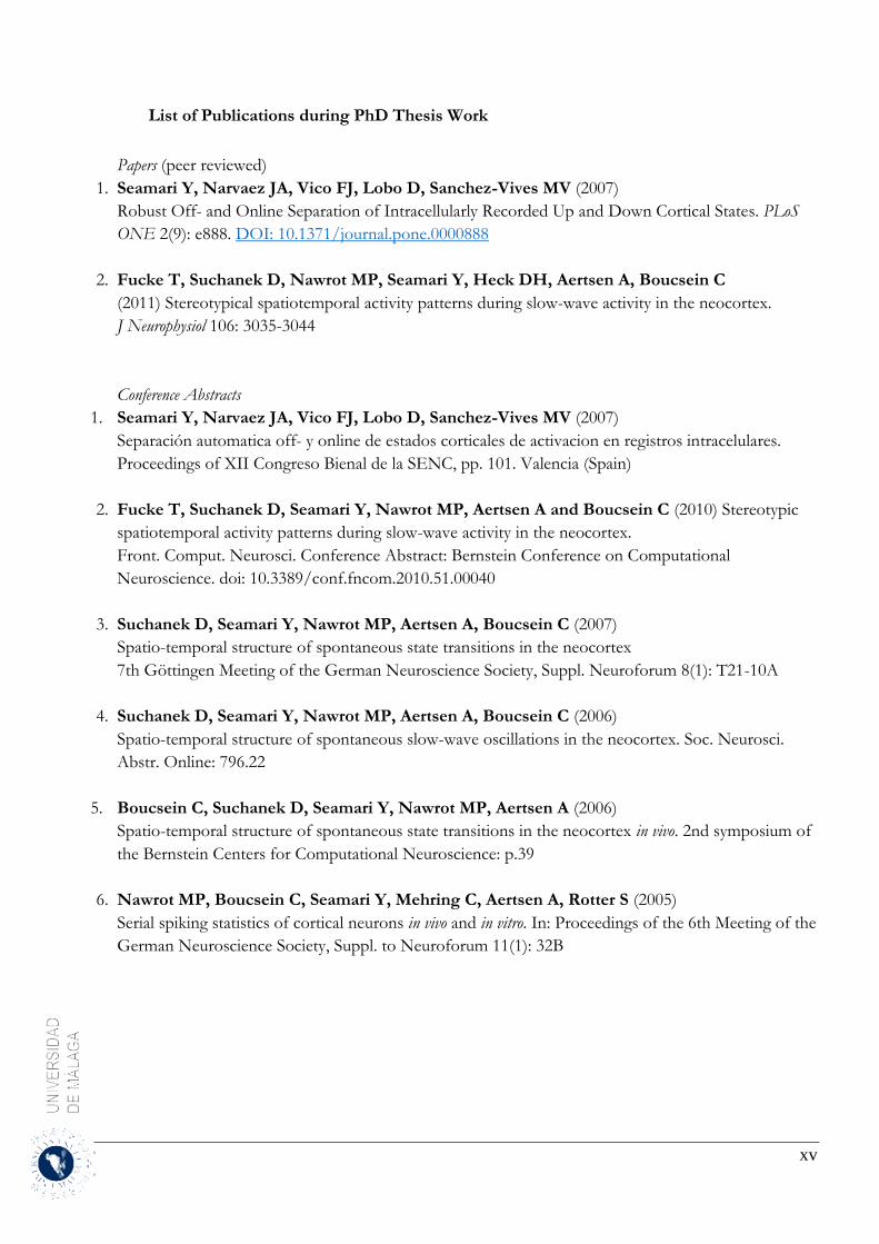
List of Publications during PhD Thesis Work
Papers (peer reviewed)
1. Seamari Y, Narvaez JA, Vico FJ, Lobo D, Sanchez-Vives MV (2007)
Robust Off- and Online Separation of Intracellularly Recorded Up and Down Cortical States. PLoS
ONE 2(9): e888. DOI: 10.1371/journal.pone.0000888
2. Fucke T, Suchanek D, Nawrot MP, Seamari Y, Heck DH, Aertsen A, Boucsein C
(2011) Stereotypical spatiotemporal activity patterns during slow-wave activity in the neocortex.
J Neurophysiol 106: 3035-3044
Conference Abstracts
1. Seamari Y, Narvaez JA, Vico FJ, Lobo D, Sanchez-Vives MV (2007)
Separación automatica off- y online de estados corticales de activacion en registros intracelulares.
Proceedings of XII Congreso Bienal de la SENC, pp. 101. Valencia (Spain)
2. Fucke T, Suchanek D, Seamari Y, Nawrot MP, Aertsen A and Boucsein C (2010) Stereotypic
spatiotemporal activity patterns during slow-wave activity in the neocortex.
Front. Comput. Neurosci. Conference Abstract: Bernstein Conference on Computational
Neuroscience. doi: 10.3389/conf.fncom.2010.51.00040
3. Suchanek D, Seamari Y, Nawrot MP, Aertsen A, Boucsein C (2007)
Spatio-temporal structure of spontaneous state transitions in the neocortex
7th Göttingen Meeting of the German Neuroscience Society, Suppl. Neuroforum 8(1): T21-10A
4. Suchanek D, Seamari Y, Nawrot MP, Aertsen A, Boucsein C (2006)
Spatio-temporal structure of spontaneous slow-wave oscillations in the neocortex. Soc. Neurosci.
Abstr. Online: 796.22
5. Boucsein C, Suchanek D, Seamari Y, Nawrot MP, Aertsen A (2006)
Spatio-temporal structure of spontaneous state transitions in the neocortex in vivo. 2nd symposium of
the Bernstein Centers for Computational Neuroscience: p.39
6. Nawrot MP, Boucsein C, Seamari Y, Mehring C, Aertsen A, Rotter S (2005)
Serial spiking statistics of cortical neurons in vivo and in vitro. In: Proceedings of the 6th Meeting of the
German Neuroscience Society, Suppl. to Neuroforum 11(1): 32B

xvi
Research Stays
I have spent a research period from 01/07/2003 to 30/06/2004 at Prof. Ad Aertsen’s Brainworks Lab,
Albert-Ludwigs-Universität Freiburg, Institut für Biologie III, Neurobiologie & Biophysik. During this
research period, I carried out a variety of research and learning activities directly related to this doctoral
thesis, including part of experiments described and data used in this thesis.
I also spent a shorter research period at the Laboratory of Prof. M.V. Sanchez-Vives, where I performed
some in vivo recordings in rat barrel cortex, at the Institute of Neuroscience of Alicante, University Miguel-
Hernández-CSIC, Spain. Part of the recordings included in this thesis were obtained in this laboratory.
xvii
Index of contents
1 Introduction .................................................................................................................................... 1
1.1 Organization of the cerebral cortex ......................................................................................... 1
1.1.1 Horizontal layers of the cerebral cortex ........................................................................... 2
1.1.2 Predominant neuron types in the neocortex ..................................................................... 3
1.1.3 Cortical columns .............................................................................................................. 4
1.2 Dynamics of the brain activity................................................................................................. 5
1.2.1 Cortical oscillations .......................................................................................................... 5
1.2.2 Nomenclature of the cortical oscillations ......................................................................... 5
1.2.3 Neural activity pattern during sleep ................................................................................. 6
1.2.4 Slow oscillations during slow wave sleep ........................................................................ 7
1.2.5 Functional role of slow oscillations ............................................................................... 11
1.2.6 The effect of anesthesia on the neuronal activity and the slow oscillation pattern ........ 12
1.2.7 Effect of ketamine anesthesia ......................................................................................... 13
1.2.8 Effect of xylazine anesthesia .......................................................................................... 14
1.2.9 Effect of urethane anesthesia .......................................................................................... 14
2 Objectives ..................................................................................................................................... 15
2.1 Aims and organization of this thesis...................................................................................... 16
2.1.1 Identification of Up and Down states ............................................................................. 16
2.1.2 Spatiotemporal structure of the slow-wave oscillation by simultaneous intra- and
extracellular recordings in vivo using a horizontal multi-electrode-array ................................... 18
3 Methods ........................................................................................................................................ 19
3.1 Detection and separation of Up and Down states .................................................................. 19
3.1.1 Experimental methods .................................................................................................... 19
3.1.2 Analytical methods ......................................................................................................... 20
3.1.3 Spatiotemporal structure of the slow-wave oscillation by simultaneous intra- and
xviii
extracellular recording in vivo using a horizontal multi-electrode-array ..................................... 26
4 Results .......................................................................................................................................... 31
4.1 Up and Down states separation using moving averages ....................................................... 31
4.1.1 Properties of MAUDS analyzing the Up and Down states ............................................ 31
4.2 Spatiotemporal structure of spontaneous slow-wave oscillations in the neocortex .............. 40
4.2.1 Down-to-Up transition ................................................................................................... 40
4.2.2 Detection of extracellular spikes .................................................................................... 44
4.2.3 Estimation of the neuronal firing rates ........................................................................... 46
4.2.4 Up-to-Down transition ................................................................................................... 60
5 Discussion .................................................................................................................................... 65
5.1 Robust off- and online separation of intracellularly recorded Up and Down cortical states. 65
5.2 Spatio-temporal structure of spontaneous slow-wave oscillations in the neocortex ............. 68
5.2.1 Constraints in experimental methodology...................................................................... 72
6 Conclusions .................................................................................................................................. 75
7 References .................................................................................................................................... 76
8 Appendix ...................................................................................................................................... 83
8.1 Protocol for in vivo experiments ............................................................................................ 83
8.2 MAUDS Programming Scripts .............................................................................................. 89

xix
List of Acronyms and Symbols
s.c. subcutaneously
i.p. intraperitonealy
ml millilitre
mg milligram
g gram
BOE Boletín oficial de estado
Fig. Figure
ECG Electrocardiogram
HEPES 4-(2-hydroxyethyl)-1-piperazineethanesulfonic acid
LFP Local field potential
PFA Paraformaldehyde
REM Rapid eye movement
SWS Slow wave sleep
CNS Central nervous system
IPSP Inhibitory post-synaptic potential
EPSP Excitatory post-synaptic potential
AP Action potential
KC K-complex
CS Cortico-striatal
MUA Multi-Unit-Activity
EU European Union
ACSF Artificial cerebrospinal fluid
CSF Cerebrospinal fluid
MAUDS
EMA
Vm
Moving average Up/Down separation
Exponential moving average
Membrane potential

xx
Introduction
1
1 Introduction
While during the 19th century most advances concerning the organization of the cerebral cortex were on
the anatomical level, during the 20th the functional aspects were investigated. Thanks to these advances, it
has been found out that the cerebral cortex is constantly active. The human brain has about 100 billion
(1011) neurons and 100 trillion (1014) connections (synapses) between them, forming a complex network
able to process in a parallel and in an organized manner inputs from all the different senses. It also sends
information to the body, thereby controlling its reactions. The neocortex, the phylogenetically more recent
part of the brain, is involved in detailed sensory perception, in performing rapid sequences of fine
movements, and in learning and intelligent behavior.
In the rat, a single pyramidal cell, the most characteristic cell type of the neocortex, receives synaptic inputs
from about 10,000 neurons (Larkman, 1991), each of which fires action potentials at an average rate
between 1 and 10 per second in vivo (Abeles et al., 1990). As a result, there is a considerable amount of
ongoing activity in the network, which is known to influence the response characteristics of individual
neurons (Arieli et al., 1996; Azouz and Gray, 1999; Tsodyks et al., 1999). Understanding the organization
of the cerebral cortex and how each neuron integrates its synaptic input, and what are the time constants
involved is crucial for the comprehension of the functioning of the network (Abeles, 1982; König et al.,
1996; Diesmann et al., 1999).
This introduction tries to give a very brief insight into the organization of the cerebral cortex and
introduces a part of the dynamics of brain activity known as cortical oscillations and revises the slow
oscillations.
1.1 Organization of the cerebral cortex
The cerebral cortex of mammals is a laminated sheet of grey matter covering the entire outer surface of
the telencephalic brain vesicles. The discovery of the highly organized structure of the cerebral cortex took
its origin from observation by Francesco Gennari in 1782, an Italian student of medicine, of a delicate pale
line (lineola albidior) running in a surface-parallel direction in the middle of the grey cortex in the medial
surface of the occipital lobe of the brain. This line was observed and illustrated by other authors of the
period (Vicq d’Azyr 1786; Sommering 1788). Indeed, the characteristic white band in the fourth layer of
the primary visual cortex is easily observable with the naked eye and still is referred to as the band of Gennari.
The basic feature of the cortical structure has been described thanks to the introduction of cell-staining
methods, first by the natural dye, carmine (Berlin, 1858), when the general arrangement of the cortical cells
in six layers (as opposed to a nuclear collection of cells) was recognized. Although the observation of
distinct cell types (pyramidal, stellate, fusiform, and granular) was already made, it was not before the
introduction of Golgi’s (1873) reazione nera (silver chromate precipitation) that the real shape of the cortical
nerve cells was fully appreciated (Golgi, 1883).
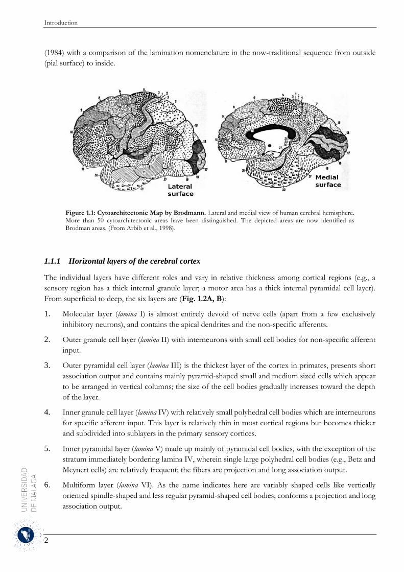
As published for the first time by Brodmann (1908, 1912, and 1914) the cerebral cortex has multiple
distinguishable areas. The cytoarchitectonic map elaborated by Brodmann (Fig. 1.1) distinguished more
than 50 areas and the basic six-layered structure of the neocortex gradually was accepted. The general
structure of the neocortex is demonstrated most elegantly and clearly in a synthetic diagram by Braak
Introduction
2
(1984) with a comparison of the lamination nomenclature in the now-traditional sequence from outside
(pial surface) to inside.
Figure 1.1: Cytoarchitectonic Map by Brodmann. Lateral and medial view of human cerebral hemisphere. More than 50 cytoarchitectonic areas have been distinguished. The depicted areas are now identified as Brodman areas. (From Arbib et al., 1998).
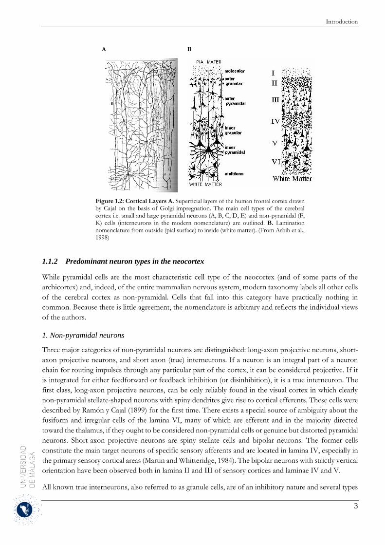
1.1.1 Horizontal layers of the cerebral cortex
The individual layers have different roles and vary in relative thickness among cortical regions (e.g., a
sensory region has a thick internal granule layer; a motor area has a thick internal pyramidal cell layer).
From superficial to deep, the six layers are (Fig. 1.2A, B):
1. Molecular layer (lamina I) is almost entirely devoid of nerve cells (apart from a few exclusively
inhibitory neurons), and contains the apical dendrites and the non-specific afferents.
2. Outer granule cell layer (lamina II) with interneurons with small cell bodies for non-specific afferent
input.
3. Outer pyramidal cell layer (lamina III) is the thickest layer of the cortex in primates, presents short
association output and contains mainly pyramid-shaped small and medium sized cells which appear
to be arranged in vertical columns; the size of the cell bodies gradually increases toward the depth
of the layer.
4. Inner granule cell layer (lamina IV) with relatively small polyhedral cell bodies which are interneurons
for specific afferent input. This layer is relatively thin in most cortical regions but becomes thicker
and subdivided into sublayers in the primary sensory cortices.
5. Inner pyramidal layer (lamina V) made up mainly of pyramidal cell bodies, with the exception of the
stratum immediately bordering lamina IV, wherein single large polyhedral cell bodies (e.g., Betz and
Meynert cells) are relatively frequent; the fibers are projection and long association output.
6. Multiform layer (lamina VI). As the name indicates here are variably shaped cells like vertically
oriented spindle-shaped and less regular pyramid-shaped cell bodies; conforms a projection and long
association output.
Introduction
3
A
B
Figure 1.2: Cortical Layers A. Superficial layers of the human frontal cortex drawn by Cajal on the basis of Golgi impregnation. The main cell types of the cerebral cortex i.e. small and large pyramidal neurons (A, B, C, D, E) and non-pyramidal (F, K) cells (interneurons in the modern nomenclature) are outlined. B. Lamination nomenclature from outside (pial surface) to inside (white matter). (From Arbib et al., 1998)
1.1.2 Predominant neuron types in the neocortex
While pyramidal cells are the most characteristic cell type of the neocortex (and of some parts of the
archicortex) and, indeed, of the entire mammalian nervous system, modern taxonomy labels all other cells
of the cerebral cortex as non-pyramidal. Cells that fall into this category have practically nothing in
common. Because there is little agreement, the nomenclature is arbitrary and reflects the individual views
of the authors.
1. Non-pyramidal neurons
Three major categories of non-pyramidal neurons are distinguished: long-axon projective neurons, short-
axon projective neurons, and short axon (true) interneurons. If a neuron is an integral part of a neuron
chain for routing impulses through any particular part of the cortex, it can be considered projective. If it
is integrated for either feedforward or feedback inhibition (or disinhibition), it is a true interneuron. The
first class, long-axon projective neurons, can be only reliably found in the visual cortex in which clearly
non-pyramidal stellate-shaped neurons with spiny dendrites give rise to cortical efferents. These cells were
described by Ramón y Cajal (1899) for the first time. There exists a special source of ambiguity about the
fusiform and irregular cells of the lamina VI, many of which are efferent and in the majority directed
toward the thalamus, if they ought to be considered non-pyramidal cells or genuine but distorted pyramidal
neurons. Short-axon projective neurons are spiny stellate cells and bipolar neurons. The former cells
constitute the main target neurons of specific sensory afferents and are located in lamina IV, especially in
the primary sensory cortical areas (Martin and Whitteridge, 1984). The bipolar neurons with strictly vertical
orientation have been observed both in lamina II and III of sensory cortices and laminae IV and V.
All known true interneurons, also referred to as granule cells, are of an inhibitory nature and several types

Introduction
4
of these inhibitory interneurons were recognized and described on the basis of their characteristic
arborisation patterns (mainly of the axons) by the classical authors, mainly Ramón y Cajal (1899) (Fig.
1.2A). Other true interneurons, like the basket cells were studied and defined more recently. The
interneurons receive input from cortical afferent fibers and form synapses on output neurons (pyramidal
cells) of the cortex. A recent classification of these complex and heterogeneous cells which includes both
anatomical and physiological types, as well as molecular features can be found in Ascoli et al. (2008).
2. Pyramidal neurons
Pyramidal neurons show a conical cell body (>30 µm in diameter) with apical and basal dendrites and an
axon that leaves the base of the cell to enter white matter. Pyramidal cells constitute the output cells of the
cerebral cortex. There is a high variation in size among pyramidal cells and they are found in virtually all
laminae, with the exception of lamina I of the cortex. The cortical pyramidal cells are arranged in an
organized way within the cortex, parallel to each other, with their apical dendrites situated perpendicularly
to the surface of the cortex, which in most cases reaches the border of the two superficial cortical layers,
I and II, wherein it breaks up into a terminal dendritic tuft. The axon of the pyramidal neuron originates
at the base of the cell body and pursues a vertically descending course. The vast majority of pyramidal cell
axons leave the cortex toward the white matter. The arborisations of the pyramidal axon collaterals are
very specific and arborize profusely in well-defined patches of the neighboring cortical tissue (Kisvárday
et al., 1986). Most dendrites of the pyramidal neurons are studded with delicate drumstick-shaped
appendages known as dendritic spines which were already described by Golgi (1883) and Ramón y Cajal
(1899) using the Golgi procedure (Fig. 1.2A). The density (number per unit length of dendrite) of the
spines, which are the receptive sites of synapses given by the terminal arborisations of terminal axon
branches, varies considerably according to species, cortical region, and type of dendrite.
Pyramidal neurons can express different electrophysiological types. The most frequent ones are regular
spiking (RS), fast spiking (FS), intrinsically bursting and chattering (or repetitive bursting) neurons (Nowak
et al. (2003) according to their electrophysiological features.
1.1.3 Cortical columns
Scheibel & Scheibel (1958) reported certain spatial regularities in the arborisation both of dendrites and of
axonal ramification in the lower brainstem, and a vertical columnar organization of the somatosensory
cortex was identified by Vernon Mountcastle (1957). Nevertheless, the observation by Hubel and Wiesel
(1959) of the so-called orientation columns in the visual cortex was even more convincing that the entire
cerebral cortex is organized into functional units. Each unit being a column (about 0.4 mm diameter)
extending the entire thickness of the cortex (including all six layers). Each vertical column is considered as
a functional unit because all cells within an individual column are activated by the same particular feature
of a stimulus. The vertical organization is the result of neuronal connections within a cortical column: Two
types of afferent projection fibers from the thalamus enter the neocortex. These are the specific afferents
which drive the modality of specific input and terminate in internal granule cell layer, exciting interneurons
which excite other neurons of the column. While the non-specific afferents, which terminate in molecular
layer on distal dendrites of pyramidal cells, are responsible to provide the background excitation to the
column. Small pyramidal cells send their axons into the white matter to excite nearby cell columns; while
large pyramidal cells (and multiform cells) send their axons into the white matter to excite distant sites via
long association fibers, commissural fibers, and corticofugal projection fibers.
Introduction
5
1.2 Dynamics of the brain activity
The brain, as a physical device, may be interpreted in terms of a dynamical system and should be considered
as a system of hierarchically arranged self-organizing structures. Self-organization is a mechanism for
generating emergent neural structures. There are different qualitative dynamic phenomena, including
oscillation, which play an important role in implementing different neural functions. The oscillations
provide a basic dynamical mode of activity in many brain regions. Oscillations may occur at the single-cell
level due to intrinsic membrane properties or may be emergent network properties resulting from the
pattern of connections between cells that are not themselves oscillators. Here, we will focus on cortical
oscillations and more specifically on the slow-wave oscillations.
1.2.1 Cortical oscillations
Since Hans Berger in 1923 placed electrodes on the skull of his son and recorded rhythmic 10 Hz frequency
waves (Berger, 1929), neurophysiological methods have advanced such that cortical oscillations of
different frequency ranges have been identified. The synchronic neuronal activity of the cerebral cortex,
which is constantly active and constituted by a huge number of neurons and synaptic connections, is
directly related to the amplitudes of the EEG waves (Contreras & Steriade, 1997).
The electroencephalography (EEG), developed by Caton at the end of the 18th century, consists in the
recording of the electrical potentials which are generated within the extracellular space by the flow of
electrical current between the interior and the exterior of the cell during neuronal activity. The EEG
displays the electrical activity originated by a current flow which is generated by the synaptic potentials of
the cortical pyramidal cells, as the action potentials are filtered by the own filter properties of the cerebral
tissue, because of their short duration. The organization of the cortical pyramidal cells, which are placed
parallel to each other and with their apical dendrites perpendicular to the cortical surface, allows the
summation of the synaptic pulses, and therefore they can be detected by the EEG electrodes placed on
the skull.
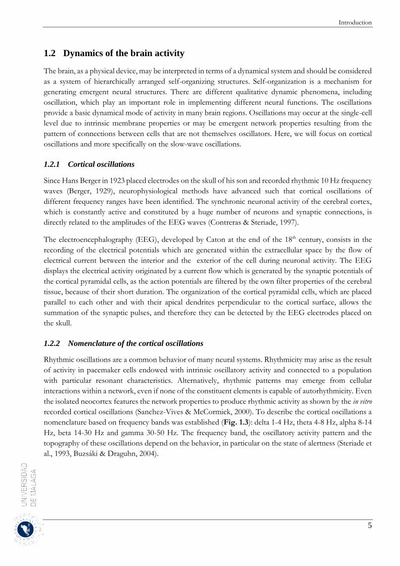
1.2.2 Nomenclature of the cortical oscillations
Rhythmic oscillations are a common behavior of many neural systems. Rhythmicity may arise as the result
of activity in pacemaker cells endowed with intrinsic oscillatory activity and connected to a population
with particular resonant characteristics. Alternatively, rhythmic patterns may emerge from cellular
interactions within a network, even if none of the constituent elements is capable of autorhythmicity. Even
the isolated neocortex features the network properties to produce rhythmic activity as shown by the in vitro
recorded cortical oscillations (Sanchez-Vives & McCormick, 2000). To describe the cortical oscillations a
nomenclature based on frequency bands was established (Fig. 1.3): delta 1-4 Hz, theta 4-8 Hz, alpha 8-14
Hz, beta 14-30 Hz and gamma 30-50 Hz. The frequency band, the oscillatory activity pattern and the
topography of these oscillations depend on the behavior, in particular on the state of alertness (Steriade et
al., 1993, Buzsáki & Draguhn, 2004).
Introduction
6
Figure 1.3: Brain Waves: EEG tracings. The
nomenclature of the different cortical oscillations
is based on the frequency bands as observed in the
EEG tracings. The frequency band, the oscillatory
activity pattern and the topography of these
oscillations depend on the behavior, in particular
on the state of alertness (Steriade et al., 1993).
(After Malvivuo and Plonsky, 1995).
1.2.3 Neural activity pattern during sleep
Three states of alertness are distinguished: slow wave sleep (SWS), REM-sleep (“paradoxical sleep” in
animals who do not move eyes) and awake state. The EEG reflects the changes of the neuronal activity
which take place during the waking state and the sleep cycle. The slow ~1 Hz EEG oscillation and the
desynchronized EEG have been related to slow wave sleep and alertness respectively (Steriade, 2000;
Steriade et al. 2001). During the waking and REM-sleep state the neuronal activity oscillates in the beta
and gamma frequency band (>15 Hz). This kind of oscillation is considered to contribute to the
information processing of the cerebral cortex.
The two stages associated with an alert brain are waking and REM. During wakefulness, brain activity is
characterized by low-voltage EEG activity and alpha waves with membrane potentials ranging between
20-40 μV occurring at a frequency of approximately 10 Hz. Due to the similar, or even greater discharge
pattern exhibited by neurons during REM sleep, both REM as well as wakefulness are active forms of
sleep. REM sleep is not only characterized by the rapid eye movements but also by a complete inhibition
of muscle tone. In contrast, non-REM sleep consists of four different stages, named stages 1-4, where
stage 1 is the transition from wakefulness to the onset of sleep, lasting only several minutes.
During both the REM-sleep and the natural waking state, rapid oscillations with small amplitudes are
generated in the beta- and gamma frequency band (40 Hz), while high amplitude oscillations appear during
the SWS showing a synchronous pattern along extent cortical areas. The activation of certain oscillatory
activity is triggered from the nuclei structures of the brainstem and the basal forebrain directly or through
the thalamus to the cortex (Steriade, 1996; Barth & MacDonald, 1996). During non-REM (NREM) sleep,
which constitutes the vast majority of sleep, neural activity is reflected in the EEG as a succession of K-
complexes, sleep spindles, and slow waves (Steriade, 2000).
Hence, the state of sleep is dominated by three major types of brain rhythms: spindles (7-14 Hz) occurring
prevalently during early stages, δ waves (1-4 Hz) appearing during later stages of sleep and slow (<1 Hz)
oscillations that are present throughout resting sleep (Steriade, 1993). The stages 2 and 3-4 of the slow-
wave-sleep (SWS) (Rechtschaffen and Kales, 1968) are characterized by oscillations in the delta frequency
band (<4 Hz), sleep spindles and K-complexes (KC) which interact leading to the characteristic EEG
pattern of the SWS. The spike rate during SWS descends representing a change of how the information is
processed. The activity of the thalamocortical system filters the flow of information to the cerebral cortex
and neuronal groups synchronize. Nevertheless, the central nervous system (CNS) continues to be alert to
Introduction
7
external sensory stimuli.
The δ rhythm consists of at least two components. The cortical one is present after thalamectomy
(Villablanca, 1974; Steriade et al., 1993). The second component is due to the capacity of thalamocortical
cells, recorded from distantly located and functionally different thalamic nuclei, to generate an intrinsic
oscillation within the δ frequency range through the interplay between two of their voltage-gated currents
and was described both in vitro (McCormick & Pape, 1990; Leresche et al., 1991) and in vivo (Steriade et al.,
1991; Curro Dossi et al., 1992). The clocklike, stereotyped δ oscillation of single thalamic cells is dissimilar
from the irregular, polymorphous EEG δ waves (the slow cortical rhythm) during natural sleep or
anesthesia which was described in intracellular recordings from a variety of sensory, motor, and
associational areas, even after extensive thalamic lesions (Steriade et al., 1993) providing evidence that the
slow oscillation is generalized at the level of the neocortex.
It was postulated that the cortical slow rhythm groups the thalamically generated (spindle and δ)
oscillations within slowly recurring wave sequences (Steriade et al., 1993). Furthermore, it was
demonstrated that thalamic spindles survive in decorticated and brainstem-transected animals (Morison
and Bassett, 1945, von Krosigk et al., 1993) and that the reticular thalamic (RE) nucleus plays a pivotal
role in their genesis and synchronization (Steriade et al., 1985, 1987).
During sleep stage 2 of spontaneous sleep and also during anesthesia with barbiturates appear the spindles
of sleep which are represented as oscillating activity at 7-14 Hz lasting for 1-2 s. The pacemaker of the
oscillating sleep spindles is situated in the reticular thalamic nucleus. The neurotransmitter released by the
neurons of the reticular thalamic nucleus is GABA, hence they are inhibitory neurons, generating
rhythmical IPSP’s in the thalamic projection neurons. The repolarization of the IPSP’s leads the thalamic
projection neurons to generate low threshold Ca2+ action potentials. The rhythmic low threshold Ca2+
action potentials in the rebound of the repolarization of the membrane potential during the IPSP event
transmit the rhythm to the cerebral cortex by generating rhythmic EPSP’s and AP’s with the same
frequency as seen in the sleep spindles and which finally can be detected by the EEG recording.
1.2.4 Slow oscillations during slow wave sleep
The slow (< 1 Hz) oscillation, as described in cortical neurons of naturally sleeping (Steriade et al., 1993;
1996) and anesthetized (Steriade et al., 1993; Cowan & Wilson, 1994; Lampl et al., 1999; Stern et al., 1997)
cats, as well as in the sleep EEG and magnetoencephalograms of humans (Achermann & Borbely, 1997;
Amzica & Steriade, 1997; Simon et al., 2000) comprises a periodic fluctuation between a hyperpolarized
membrane potential or Down state, characterized by the absence of network activity, and a depolarized
membrane potential, or Up state where action potentials use to occur.
During the hyperpolarization phase or Down state virtually all cortical neurons are deeply hyperpolarized
and remain silent for a few hundred milliseconds. Whereas during the Up state, the membrane potential
surges back to firing threshold, the entire thalamocortical system is seized by intense synaptic activity, and
neurons fire at rates that are even higher than in quiet wakefulness (Steriade et al., 2001).
The Up state is hence associated with the arrival of a barrage of excitatory and inhibitory postsynaptic
potentials leading to the discharge of both excitatory and inhibitory neurons. The Down state periodically
interrupts the Up state with membrane potentials ~10.4 ± 4.94 mV more hyperpolarized compared to the
active Up state.
Introduction
8
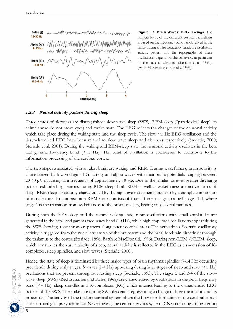
Because of the absence of any network activity during this Down state, it is also known as the quiescent
period and is associated with a disfacillitation of the network (Sanchez-Vives & McCormick, 2000;
Massimini & Amzica, 2001). The changes in membrane potential as well as firing pattern during
wakefulness, SWS and REM are nicely depicted in Fig. 1.4.
Figure 1.4 Changes in membrane potential during different stages of alertness. Awake, SWS, and REM sleep for a regular-spiking neuron located within the suprasylvain gyrus (area 21) of the cat. Simultaneous EEG and EMG recordings from area 5 are also shown. The horizontal bars below the intracellular trace indicate the time intervals expanded underneath. Noticeable are the tonic firing rates during both the waking state and REM sleep, whereas during SWS, characteristic cyclic hyperpolarizations associated with depth-positive field potentials in the EEG, make this phase unique. (From Steriade et al. 2001)
The mechanisms ruling the switch between these two states are still poorly understood but has been
described in virtually all cortical neurons (Massimini & Amzica, 2001; Volgushev et al., 2006) and shows a
frequency between 0.5 and 0.8 Hz (Sanchez-Vives & McCormick, 2000). Both phases of the slow
oscillation are synchronous over large cortical territories (Amzica & Steriade, 1995). The persistent
depolarization’s reflecting synchronous excitations within large neuronal populations are reflected
extracellularly as negative field potentials (Contreras & Steriade, 1995). The vertical disposition of apical
dendrites belonging to pyramidal neurons makes these deep currents revert at the cortical surface. Thus,
the depolarizing phase of the slow oscillation is associated with a superficial positive wave of the EEG,
which is the first component of the KC, i.e. it is associated with the arrival of a barrage of excitatory and
inhibitory postsynaptic potentials leading to the discharge of both excitatory and inhibitory neurons. The
second component of the slow oscillation during which the membrane potential of cortical neurons is
hyperpolarized, is due to the progressive decrease of extracellular Ca2+ concentration (Massimini &
Amzica, 2001) inducing diminished synaptic efficacy and general disfacilitation in the cortical network
(Contreras et al., 1996). The synchronous hyperpolarization of the neurons is reflected in the depth field
potential as a positive wave and at the cortical surface as a negative wave (Contreras & Steriade, 1995).
Hence, the KC’s appear rhythmically with a frequency of >1Hz (mainly 0.6-0.9 Hz).
The slow oscillation is cortically generated (Steriade et al., 1993b) and takes place as a stable synchronous
network event as demonstrated by multiple intra- and extracellular recordings in the intact brain (Amzica
& Steriade, 1995; Massimini et al., 2004; Volgushev et al., 2006). Its generation by the cortical network is
Introduction
9
supported by the fact that it is also generated in deafferented cortical slabs (Timofeev et al., 2000) and in
cortical slices maintained in vitro (Sanchez-Vives & McCormick, 2000). Thus, the low oscillation is initiated,
maintained and terminated through the interplay of intrinsic currents and network interactions, as shown
by studies in vivo (Timofeev et al., 2000; Ruiz-Mejias et al., 2011), in vitro (Sanchez-Vives & McCormick,
2000), and in computo (Bazhenov et al., 2002; Compte et al., 2003; Mattia & Sanchez-Vives, 2012). It can be
generated and sustained by the cerebral cortex alone (Steriade et al., 1993b; Timofeev & Steriade, 1996;
Timofeev et al., 2000; Shu et al., 2003) and is disrupted by disconnection of intracortical pathways (Amzica
& Steriade, 1995). A large number of studies have been published in recent years dealing with the cellular
and network mechanisms underlying this slow rhythm and other related aspects, such as the effect of Up
and Down states on synaptic transmission and excitability (Azouz & Gray, 1999; Crochet et al., 2005;
Haider et al., 2006; McCormick et al., 2003; Petersen et al., 2003; Sachdev et al., 2004; Timofeev et al.,
1996; Reig et al., 2015; Reig & Sanchez-Vives, 2007).
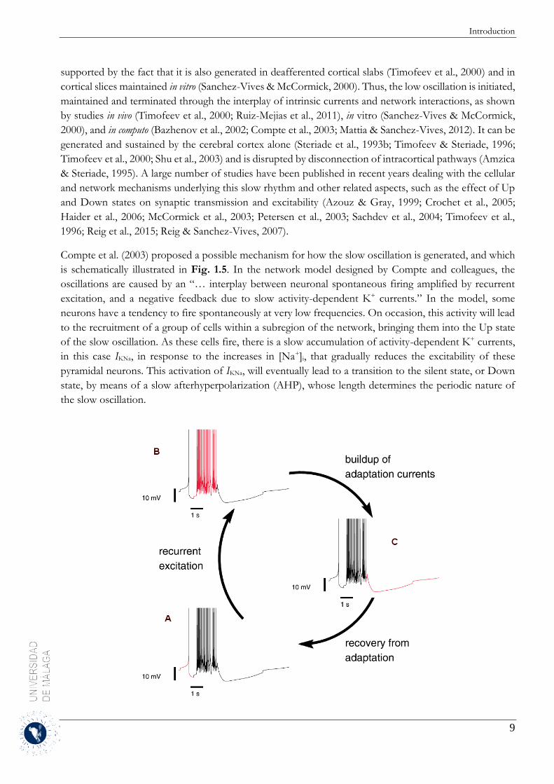
Compte et al. (2003) proposed a possible mechanism for how the slow oscillation is generated, and which
is schematically illustrated in Fig. 1.5. In the network model designed by Compte and colleagues, the
oscillations are caused by an “… interplay between neuronal spontaneous firing amplified by recurrent
excitation, and a negative feedback due to slow activity-dependent K+ currents.” In the model, some
neurons have a tendency to fire spontaneously at very low frequencies. On occasion, this activity will lead
to the recruitment of a group of cells within a subregion of the network, bringing them into the Up state
of the slow oscillation. As these cells fire, there is a slow accumulation of activity-dependent K+ currents,
in this case IKNa, in response to the increases in [Na+]i, that gradually reduces the excitability of these
pyramidal neurons. This activation of IKNa, will eventually lead to a transition to the silent state, or Down
state, by means of a slow afterhyperpolarization (AHP), whose length determines the periodic nature of
the slow oscillation.

Introduction
10
Figure 1.5: Possible mechanism for the slow oscillation. Possible mechanism for the slow oscillation. Starting at A in the depicted schematic, due to a lower firing threshold, some neurons will fire spontaneously. This spontaneous activity can lead to the recruitment of additional neurons and thus a transition into the Up state as seen in B. During the Up state, the IKNa current gradually builds-up until neuronal excitability has decreased to such an extent that the Up state cannot be maintained and a switch to the Down state is made, C. The length of the AHP, determines the periodicity of the slow oscillation. (From Compte et al. 2003)
Hence, the authors assumed that the activity dependent slow IKNa current is actually the agent responsible
for the switching between the Up and the Down states. They tested their prediction by blocking the time-
varying Na+-dependent K+ channels and substituting their activity by injecting constant hyperpolarizing
current pulses. Indeed, the network was found to exhibit two stable states. During the Up state, IKNa slowly
accumulates leading the pyramidal neurons to experience a hyperpolarization that will cause a sudden
transition to the Down state due to the loss of network stability. As IKNa gradually recovers, this enables
the network to transition to the Up state once again and driven by the kinetics of the activity-dependent
K+ currents, the so-called bi-stability loop emerges.
In summary, it has been shown that in the emergent oscillatory activity of the cerebral cortex excitation
and inhibition (Shu et al., 2003; Compte et al., 2009) and activity-dependent adaptation mechanisms
(Compte et al., 2003; Sanchez-Vives et al., 2010; Mattia & Sanchez-Vives, 2012) determine that levels of
activity are maintained during cortical function. Precisely, Mattia & Sanchez-Vives showed that three
critical elements in a model network characterized by mean-field approximation characterizes this
emergent property. These key elements are i) synaptic reverberation in neuronal networks together with
nonlinear amplification, ii) two attractor states of low and high firing rate that embody intrinsic fluctuations
and iii) additional activity-dependent mechanism of self-inhibition. The balanced interplay of these three
key elements eventually yield to a so-called “relaxation oscillator” capable to fit experimental evidence and
representing the slow oscillation as a dynamical regime of the cortical tissue in which episodes of stable
network states (Up and Down states), emerge for short time periods, as shown in Fig. 1.6.
Figure 1.6: Slow oscillations between stable network states as a relaxation oscillator. Black curve depicts the firing rates at the fixed points (circles) of the attractor dynamics. The solid and dotted branches correspond to stable or unstable fixed points. Recurrent stable (solid branches) and unstable (dotted branch) asymptotic states of firing rate (v) at different fatigue levels are represented as effective changes in the input current ΔI to the neurons in the network. The gray line is the nullcline where the fatigue level is expected to be fixed in time and provides the amount of self-inhibition. (Figure adapted from Mattia & Sanchez-Vives, 2012)
It is well known that several neuromodulators are involved in the regulation of the brain’s state of vigilance
and that the transition from sleep to wakefulness depends critically on the activation of ascendent
activating systems, including acetylcholine (ACh), norepinephrine, and serotonin (McCormick 1992;
Introduction
11
Steriade et al., 1997). The activation of certain neuromodulatory systems, such as increasing the level of
ACh can reduce the K+ conductances, including the Na+-dependent K+ conductance, reverting the
oscillating network activity with less marked periodicity, longer Up states and shorter Down states until
the state of tonic firing resembling the voltage traces of the waking state. In the model depicted in Fig.
1.6 the characteristic neurophysiological differences between the SWS and the waking states could only be
resembled closely by changing different parameters of excitation and inhibition (Shu et al., 2003; Compte
et al., 2009) and activity-dependent adaptation mechanisms (Compte et al., 2003; Sanchez-Vives et al.,
2010; Mattia & Sanchez-Vives, 2012). Nevertheless, the enhancement of the neuromodulatory effect
enters the network eventually into a tonic firing state with no large-scale spatio-temporal coherence,
reminiscent of typical cortical activity in the awake state (Destexhe et al., 1999; Steriade et al. 1996), recently
observed also in a thalamocortical network model of slow oscillations (Bazhenov et al., 2002).
An additional point of interest is that the periodic fluctuations in membrane potential occurring during
SWS do also conduct to fluctuating changes in the ionic composition both within the extracellular as well
as the intracellular medium. Intracellular calcium concentrations are usually kept very low (1-1.3 mM), thus
even small changes in its concentration can lead to large effects. Extracellular measurements using an ion-
sensitive microelectrode showed phasic fluctuations in [Ca2+]out (Massimini & Amzica, 2001). The
minimum concentration (~0.9 mM) coincided with the end of the depolarizing phase followed by an
almost linear increase after onset of the hyperpolarizing phase, reaching values of about 1.2 mM. The
authors in this study believe, that because of the periodic depletions of [Ca2+]out, synaptic depression is
caused and a concomitant transition to the Down state, while during the silent phase the resting levels of
calcium are restored and with it the synaptic efficacy.
It remains still to be determined, whether the calcium balance or the kinetics of Na+-dependent K+
conductance are responsible for the switching between active and silent states but evidence points toward
a combination of the two as the most likely scenario (Volgushev et al., 2005).
During the Up state, external calcium levels are depleted (by almost 20%) due to the possible inflow of
the divalent cation via N-type Ca2+ channels located near the active zones (Kandel et al., 2000). This
contributes to the gradual decrease in conductance, thus a simultaneous increase in the input resistance
(Rin) during the Up state. While the overall conductance is decreasing, IKNa currents start building Up with
only minimal effects on the overall conductance. Due to a loss of network stability, neurons will not be
excitable enough to maintain the Up state and thus a sharp transition to the Down state is made. Whereas
during this hyperpolarized state, [Ca2+]out can be restored and recurrent excitation is able to drive the
network into the Up state once again (Compte et al., 2003).
1.2.5 Functional role of slow oscillations
Another interesting question that remains to be answered is, what is the functional significance of the
persistent slow oscillating activity in the cortical network? Most authors propose that the high rates of
firing during the active states of slow wave sleep, which lead to a bombardment of target neurons by both
rhythmic spike trains as well as spike bursts, may lead to spike-dependent synaptic plasticity processes
(Steriade et al., 2001; Massimini et al., 2004). Slow oscillation could thus be essential for memory
consolidation whereby memory traces acquired during wakefulness are preferentially processed (Mukovski
et al., 2007; Steriade et al., 2001).
Memory is classified into two fundamental forms: explicit (also termed declarative) and implicit (also
Introduction
12
termed non-declarative), respectively (Stickgold & Walker, 2005). The first involves consciously accessible
memories of fact-based information, i.e. knowing “what”, and contains several subcategories, including
episodic memory (memory for events in one’s past) and semantic memory (memory for general
knowledge). By contrast, non-declarative memory includes all non-conscious memories, and has
subcategories such as conditioning, implicit memory and procedural memory (i.e. knowing “how”). Or
said shortly; it’s the memory of how a certain task or skill is performed, such as hitting a tennis ball. Thus,
during different phases of sleep, traces of these different memory types, declarative as well as non-
declarative are differentially processed leading to synaptic consolidation or downscaling (Mukovski et al.,
2007; Steriade et al., 2001). Evidence of sleep-dependent plasticity at both local and system levels suggests
that sleep has a crucial role in consolidation processes leading to memory enhancement (Stickgold &
Walker, 2005).
Another approach for the functional role of slow oscillations determined using computational models, has
been that they might be responsible for the persistent activity of neurons in the prefrontal cortex of
primates while they are performing delayed-response memory tasks. In the primary visual cortex, where
this spontaneous activity has been investigated in detail in cortical slices of the ferret, it might be that this
activity; at least in some cell types, is important for the generation of receptive field properties (Sanchez-
Vives & McCormick, 2000).
The precise function role of these alternating states still remains an enigma and the approaches mentioned
above still need to be investigated further. This gives rise to the question, how can we elicit these rhythmic
alternations in membrane potential artificially so that it can be studied more easily?
1.2.6 The effect of anesthesia on the neuronal activity and the slow oscillation pattern
Due to the wide interest in the function; both on a cellular as well as a mechanistic level, of slow oscillations
in humans as well as animals, two methods enable us to artificially induce this rhythm (<1 Hz) both under
in vitro as well as in vivo conditions. Traditional slice bathing mediums (2 mM Ca2+, 2 mM Mg2+ and 2.5 mM
K+) used to maintain cortical slices under in vitro conditions do not show spontaneous rhythmic
oscillations. However, when changing the ionic concentrations of the ACSF such that they resemble more
closely the composition of the brain interstitial fluid (1-1.2 mM Ca2+, 1 mM Mg2+ and 3.5 mM K+), these
spontaneous slow oscillations appear. The membrane potential distribution again showed the characteristic
bimodality, with Up states exhibiting spiking frequencies of 2-10 Hz and Down states occurring
approximately every 3.4 s (Compte et al., 2003; Sanchez-Vives & McCormick, 2000).
It has been shown that activity in cortical cells is critically dependent on the type of anesthesia, i.e. different
anesthetics inducing distinctive cortical rhythms mimicking different sleep stages (Steriade, 1997). Hence,
concerning anesthesia during electrophysiological experiments there is often the need to find a
compromise between a sufficient depth of anesthesia and the alteration of the neuronal activity. The depth
of anesthesia is controlled by monitoring different parameters like: the breath and pulse frequency, the
EEG, the involuntary responses of the muscles to stimulations like pain and the opening of the pupil.
Under certain anesthetics, the neuronal activity shows slow oscillations similar to that observed during
slow wave sleep. These anesthetics are ketamine, urethane and halothane.
As discussed in the former section, slow oscillation consists of long-lasting depolarizations with
superimposed action potentials, separated by long periods of neuronal silence which is closely related with
a similar rhythm of EEG waves. These slow cortical potentials are similar to the slow oscillations present
throughout resting sleep in mammals and in urethane or ketamine-xylazine-anesthetized cats (Steriade,
Introduction
13
1993; Steriade et al., 1993a, 1993b; Contreras & Steriade, 1995) and could be observed under all (but deep
barbiturate) anesthetic conditions, as well as in high brainstem-transected undrugged preparations. Mahon
et al. (2001) performed a study in vivo where the three different anesthetics used induced EEG waves that
were associated with dissimilar patterns of activity in cortico-striatal (CS) neurons. The different patterns
of cortical activity described by Mahon et al., 2001 did not result from an anesthetic dependent alteration
in intrinsic membrane properties of cortical neurons and no significant difference in the basic electrical
features of CS cells recorded under the different anesthetics could be observed.
The basic difference between neuronal oscillations recorded under urethane and those under ketamine
was the frequency of the rhythm. Thus, under urethane anesthesia mainly slow oscillations with a
frequencies in the range of 0.3 to 0.4Hz with overwhelming pattern of spindling activity were presented
while ketamine showed mostly 0.6-1 Hz, i.e. a pronounced shift toward higher frequencies.
1.2.7 Effect of ketamine anesthesia
Ketamine (Ketanest®) belongs to the dissociative anesthetics producing hypnotic, analgesic and amnesic
effects, i.e. it is sleep producing, pain relieving and causes a short term memory loss. These effects are
conducted without the actual loss of consciousness but leading to a state of cataleptic immobility.
Ketamine and other dissociative anesthetics selectively block the NMDA subtype of excitatory aminoacid
receptor (MacDonald et al., 1991), thus, selectively decreasing synaptic transmission at terminals of
excitatory neurons. The mechanism of action is the blocking of ion channels of non-competitive N-
methyl-D-aspartate (NMDA) (Anis et al., 1983) receptors without substantial alteration of the function of
γ-aminobutyric acid type A (GABAA), glycine, and α-amino-3-hydroxy-5-methyl-4-isoxazole propionic
acid receptors (AMPA). Ketamine increases the monoaminergic transmission and induces the inhibition
of voltage-gated sodium channels by agonistic effects on the opiate receptors. EEG records exhibit a slow
rhythm at ~ 1Hz.
Dissociative anesthesia is a stage whereby somatic analgesia is combined with a light plane of
unconsciousness, but the animal seems dissociated from its environment. During the dissociative
anesthesia, the respiratory function remains stable and the animal maintains its pharyngeal, laryngeal,
corneal, palpebral and swallowing reflexes. The eyes remain open. Dissociative anesthetic agents increase
muscle tone and spontaneous involuntary muscle movements (occasionally seizure) are common due to
its poor muscle relaxant properties and variable analgesia. Salivation and lacrimation are also increased.
Ketamine has potent sympathomimetic effects like hypertension, increase of the heart pulse frequency and
myocardial consumption of oxygen as well as bronchodilatation. At recommended dosages, ketamine
causes minimal depression of the respiratory and cardiovascular systems, but is a poor muscle relaxant in
most species. When used in guinea pigs (at a dosage of 55 mg/kg i.p.), however, ketamine alone may
provide muscle relaxation sufficient for restraint and manipulation for procedures which impart minimal
pain to the animal. This is one of the few situations in which ketamine, alone, is a suitable anesthetic in
rodents. The onset of action when applied via intravenous (i.v.) occurs after seconds, while it takes about
5 minutes when applied via injection into the muscle. Due to its poor muscle relaxant properties in other
species of rodents, ketamine is often combined with tranquillizers, such as xylazine, acetylpromazine,
diazepam, and butorphenol to facilitate muscle relaxation. The ketamine-xylazine combination provides
better analgesia than does ketamine-diazepam or ketamine-acetylpromazine. Ketamine-xylazine should be
used with caution at high dosages, however, because it produces respiratory and cardiovascular depression,
Introduction
14
hypothermia, and can produce muscle necrosis when injected by the i.m. route.
1.2.8 Effect of xylazine anesthesia
Xylazine is an alpha-2 adrenergic agonist (Nicoll et al., 1990) acting at alpha-2 adrenoreceptors to inhibit
neurotransmitter release at sympathetic and parasympathetic nerve endings. It is used as a sedative,
analgesic, and muscle relaxantin veterinary medicine. Its sedative and analgesic properties are related to
nervous system depression, acting on presynaptic and postsynaptic receptors of the central and peripheral
nervous systems. Its effects include bradycardia, hypotension due to activation of alpha-2 adrenoreceptors
in medullary pressor centers and resulting depression of sympathetic outflow from these centers, and
inhibition of the effects of postganglionic nerve stimulation. Overall it produces respiratory and
cardiovascular depression and hypothermia. In veterinary anesthesia, xylazine and ketamine are often used
in combination. Ketamine, unlike xylazine, is used in both humans and other animals. When xylazine is
used in combination with ketamine it may cause muscle necrosis at the i.m. injection site, therefore, i.p.
injection is recommended.
1.2.9 Effect of urethane anesthesia
Urethane (ethyl carbamate) is a water-soluble compound widely used as an anesthetic in animal
experiments. It is also a carcinogen, which precludes its use as a human anesthetic. The advantages of
urethane in animal anesthesia are that it can be administrated by several parenteral routes, produces a long-
lasting steady level of surgical anesthesia, and has minimal effects on autonomic and cardiovascular
systems. Recent studies in rodents have shown that it has a rapid onset after i.p. administration, which is
followed by hypotension, hypothermia, bradycardia and metabolic acidosis with partial respiratory
compensation. Advantages of urethane anesthesia are that it produces good muscle relaxation and
analgesia sufficient for surgical manipulations. Urethane has also been shown to produce sedation and
ataxia following topical administration to rodents. The primary disadvantages of urethane are that it is a
proven carcinogen and mutagen in rodents, therefore, its use is strongly discouraged unless strict
precautions are taken (e.g. gloves, face masks, mixing under a fume hood) to protect personnel. Due to its
mutagenic and carcinogenic potential, use of urethane should be limited to non-survival procedures.
Urethane has been reported to affect both inhibitory and excitatory neurotransmission systems and the
magnitude of the change is less than that seen with anesthetics that are more selective for one system (e.g.,
ketamine and NMDA receptor). The functions of GABAA and glycine receptors are enhanced while the
NMDA and AMPA receptors are inhibited by the action of urethane (Hara & Harris, 2002). Furthermore,
urethane interestingly enhances the function of the nACh receptor.

Objectives
15
2 Objectives
The general objective of this thesis is to learn about the dynamics of the cortical network through its
slow oscillatory emergent activity.
In order to achieve this objective, I have devoted a large part of the efforts in this thesis to the development
of methodological tools that allow myself and others to identify and explore the properties of oscillations.
In an approach to this objective, three more specific objectives can be resumed as follows:
- To develop a method that allows the detection and idenfication of cortical Up and Down states in
intracellular recordings.
- To investigate the spatiotemporal properties of wave propagation during slow wave activity on a
micro- to mesoscopic scale by developing adequate analytical tools.
- To examine the stereotypical behavior of spontaneous transitions between Up and Down states in
the somatosensory cortex of anesthetized rats.

Objectives
16
2.1 Aims and organization of this thesis
In order to tackle these specific objectives this thesis is divided into two blocks:
1. The first block refers to the definition, formalization, implementation and analysis of an easy to use
method for Up and Down states detection and identification in intracellular recordings.
2. The second block describes the information obtained from simultaneously recorded intra- and
extracellular signals using a multi-electrode array and analyzes the spatiotemporal structure of the
slow oscillation within a small portion of cortical tissue covered by the extracellular matrix and
triggering on the intracellular signal. In particular, the analytical tools developed and applied for this
study are emphasized and described in detail.
2.1.1 Detection and Identification of Up and Down states
Once the simultaneous intra- and extracellular data have been recorded, we proceeded to correctly and
reliably detect and identify the Up and Down states of the slow cortical oscillations. For further detailed
data analysis, it is often required to detect, identify and quantify the Up and Down states, in order to
respond to questions regarding the integrative or synaptic properties of cortical cells during slow
membrane potential fluctuations. To achieve this processing of intracellularly recorded membrane
potential fluctuations some methods deal with the data in a manual fashion, while others implement basic
automated procedures.
Metherate and Ashe (1993) first carried out the quantification of the two-state behavior based on the
membrane potential distribution. That graphical tool operates on the characteristic bimodal distribution
of the membrane potential, best fitted to a dual Gaussian function, and has been extensively used since
then (Sanchez-Vives & McCormick, 2000; Petersen et al., 2003; Anderson et al., 2000; Benucci et al., 2004;
Crochet et al., 2004; Fuentealba & Steriade, 2005; Holcman & Tsodyks, 2006; Kasanetz et al., 2002; Lewis
and O’Donnell, 2000; Mahon et el., 2003; Peters et al., 2004; Timofeev et al., 2001; Tseng et al., 2001). A
peak at the hyperpolarized membrane potential values identifies the Down state, separated from the
depolarized Up state by a well-defined central valley, indicative of fast transitions between the two states.
Recently, a moving average of the membrane potential and its standard deviation (StD) has been presented
(Volgushev et al., 2006) to separate the two states. In this case the Down state presents a sharp peak at
hyperpolarized potentials with low StD values, while the Up state shows a broader hill at more depolarized
potentials and higher StD values. A different approach based on the spectral difference of the local field
potential (LFP) signal has been recently proposed to distinguish between Up and Down states (Mukovski
et el., 2007). This method also relies on the bimodal distribution of the membrane potential.
The basic assumption underlying the approaches based on the bimodal distribution of the membrane
potential is that the proportion of the area of the histogram under each of the peaks represents the
proportion of time spent in each state, and consequently the mode of each peak is the preferred membrane
potential in each state. While this is true for very stable recordings, data is typically affected by fluctuating
electrical and physiological conditions.
According to this property, these approaches proceed by performing certain measurements on the biphasic
histogram. A basic operation is to determine the threshold potential that delimits both states. This is
obtained by computing the modes of the distributions (or, alternatively, visually identifying the peaks) and

Objectives
17
finding either the potential associated with the lowest bar between them, or the midpoint between the
peaks if a broad valley separates them (Wilson & Kawaguchi, 1996). More reliable transitions can be
performed by setting two thresholds, e.g., at one fourth and three fourths of the distance between the
peaks (Anderson et al., 2000). The areas separated by these delimiting values are a good estimation of the
time spent in each mode.
Despite the simplicity and popularity of the histogram-based methods, there are some disadvantages
related to its use:
1. The intracellular membrane potential recordings must be stable over the time window used to
compute the histogram. However, this ideal scenario is frequently complicated by membrane
potential drift, changes in the electrode seal, movement artifacts (e.g. respiratory movements,
heartbeat) or other factors, particularly when large time spans are to be considered. These changes
will tend to blur the standard bimodal distribution of Up and Down states, making it hard to
separate the two states based simply on threshold.
2. Although the threshold can be automatically determined, there is a certain tendency to establish
the settings manually according to the expert assessment, even when dealing with very stable
recordings and well-differentiated bimodal behavior. A reliable computerized method for peak
identification in the histogram of membrane potentials from recordings that are not obtained in
ideal conditions could be hard to find.
An increasing amount of “non-standard” electrophysiological data (from anesthetized animals and slice
recordings) and in addition long duration recordings demand automated and reliable methods for Up and
Down states identification and characterization. We present an automatic and easy-to-use method that is
able to identify and to reliably separate the two states of membrane potential, characteristic of slow wave
sleep and under certain anesthesia: MAUDS (for Moving Averages for Up and Down Separation).
Furthermore, the method has been engineered to be used online, in such a way that the Up and Down
states can be visualized in real-time superimposed to the original signal, and the experiment design can
include triggering events. It also provides immediate information on the statistics of the Up versus Down
periods to evaluate the behavior of the network.
Objectives
18
2.1.2 Spatiotemporal structure of the slow-wave oscillation by simultaneous intra- and
extracellular recordings in vivo using a horizontal multi-electrode-array
Propagating waves of activity within neocortical networks are a phenomenon that can be observed under
many different conditions, from strong sensory stimulation in various primary sensory areas such as barrel
cortex (Ferezou et al. 2006; Petersen et al. 2003), visual cortex (Xu et al. 2007), and motor cortices (Rubino
et al. 2006), as well as during the slow-wave sleep (Chauvette et al. 2010) and anesthesia-induced slow-
wave activity (Steriade et al. 1993a; 1993b; 1993c; Takagaki et al. 2008). Although this phenomena is so
widespread, there is a strong interest in understanding the mechanisms underlying wave propagation in
the neocortex while the functional role of the traveling waves still remains unclear.
The results from in vitro cortical slices have achieved important insights in the intrinsic and synaptic
properties of various neuronal types and different cortical areas. Slice preparations permit a complete
control of the ionic composition of the bath solution and a good visualization of the electrodes within the
tissue. It was emphasized (Chagnac-Amitai & Connors, 1989) that small regions of neocortex could sustain
synchronous activity, but it was not proven until Sanchez-Vives & McCormick (2000) demonstrated that
maintaining the ionic concentration of the ACSF bath solution for the slices in situ-like sustained slow
oscillation can be observed. However, inevitably many dendrites are lopped when the slice is prepared and
in vitro preparations lack a complete cortical network.
Experiments in vivo assure a complete cortical network with all inputs and background activity. Usually
they are focused on cellular responses to different sensory modalities and during alert preparations, thus
requiring alert preparations, which does not show slow oscillation of the brain electrical activity. Thus, to
get slow oscillations in vivo it is required to record either during sleep of the subject or using certain
anesthetics like ketamine, urethane, fentanyl or halothane. The slow oscillation, recorded under slow wave
sleep and under anesthesia, represents a spontaneous event during which cortical neurons are alternately
silent and active for a fraction of a second.
Because traveling waves generate spatiotemporal patterns during slow-wave activity, we were interested
on the spatiotemporal structure of the spontaneous slow-wave in the rat’s somatosensorial neocortex
under ketamine/xylazine anesthesia and on how and to what extent the activity spread through the
neocortical network. Studies performed in the anesthetized rat implementing voltage-sensitive dye (VSD)
imaging have shown that activity waves have a tendency to propagate along specific paths, even showing
cross-modal activation (Takagaki et al. 2008). EEG studies in humans also revealed an origin and
preferable direction of wave propagation that was consistent across subjects (Massimini et al. 2004; Riedner
et al. 2007). On the other hand, VSD imaging performed in the barrel cortex of awake mice indicated that
spontaneous waves varied their direction from one trial to the next (Ferezou et al. 2006).
In order to shed light to this matter, we first need to investigate how slow oscillations, present during
certain anesthetics, propagate along a small cortical area. Subsequently, we need to answer the question of
how the extra- and intracellular signals of these oscillations correlate with each other. With that purpose,
we carried out extracellular recordings using a spatially defined array of seven extracellular electrodes in
combination with one intracellular electrode and recorded from the somatosensory cortex of rats
anesthetized with urethane and ketamine/xylazine. This kind of anesthesia has been established as a model
for slow-wave sleep (Fontanini et al. 2003; Sharma et al. 2010) and leads to stable and regular low-frequency
oscillations in the neocortex. In order to get correlated data and to cover a very small (microscopic) portion
of cortical tissue, the intracellular electrode and the multi-electrode array were positioned close to each

Objectives
20
other.
Methods
19
3 Methods
We used intra- and extracellular data obtained by recordings in different cortical areas and preparations. A
part of the data used for implementation and analysis of the developed method MAUDS were kindly
provided by the Laboratory of Prof. M.V. Sanchez-Vives (slice preparations and the majority of the in vivo
recordings in rat barrel cortex) at the Institute of Neuroscience of Alicante, University Miguel-Hernández-
CSIC, Spain. The methods followed to record this data are described briefly in the following section and
were published in PLOS One (2007) which is attached in the appendix section of this thesis (Seamari et al.,
2007).
The experimental procedure followed by the author of the present thesis at Albrecht-Ludwigs-University of
Freiburg, Germany, in order to obtain combined extra-intracellular recordings at the rat’s somatosensorial
cortex is described below in detail and was carried out by the author of this thesis. The legends of all
figures indicate the origin of data. The experimental setup, implementation and part of the results described
in this thesis were published in Journal of Neurophysiology (2011), paper which is attached to this document
(Fucke et al., 2011).
3.1 Detection and Identification of Up and Down states
3.1.1 Experimental methods
For the detection and identification of Up/Down states, data from three different preparations were used:
brain slices, cat visual cortex and rat barrel cortex.
Animals were cared for and used in accordance with the Spanish regulatory laws (BOE 256; 25-10-1990)
which comply with the EU guidelines on protection of vertebrates used for experimentation (Strasbourg
3/18/1986).
Slices preparation
The cortical slices were prepared from 2- to 6-month-old ferrets of either sex that were deeply anesthetized
with sodium pentobarbital (40 mg/kg) and decapitated. Four hundred-micrometer-thick coronal slices of
the visual cortex were cut on a vibratome. After preparation, slices were placed in an interface-style
recording chamber and bathed in ACSF containing (in mM): NaCl, 124; KCl, 2.5; MgSO4, 2; NaHPO4,
1.25; CaCl2, 2; NaHCO3, 26; and dextrose, 10, and was aerated with 95% O2, 5%CO2 to a final pH of 7.4.
Bath temperature was maintained at 34–35ºC. Intracellular recordings were initiated after 2 hour of
recovery. In order to induce spontaneous rhythmic activity, the solution was switched to ACSF containing
(in mM): NaCl, 124; KCl, 3.5; MgSO4, 1; NaHPO4, 1.25; CaCl2, 1–1.2; NaHCO3, 26; and dextrose, 10
(Sanchez-Vives & McCormick, 2000).
Intra- and extracellular recordings were obtained from the slices as described below:
Animal preparation for in vivo recording
For the intracellular recordings in vivo from the primary visual cortex, adult cats were anesthetized
with ketamine (12–15 mg/kg, i.m.) and xylazine (1 mg/kg, i.m.) and then mounted in a stereotaxic frame.

Methods
20
A craniotomy (3–4 mm wide) was made overlying the representation of the area centralis of area 17. To
minimize pulsation arising from the heartbeat and respiration a cisternal drainage and a bilateral
pneumothorax were performed, and the animal was suspended by the rib cage to the stereotaxic frame.
During recording, anesthesia was maintained with i.m. injections of both ketamine (7 mg/kg) and xylazine
(0.5 mg/kg) every 20–30 min. The heart rate, expiratory CO2 concentration, rectal temperature, and blood
O2 concentration were monitored throughout the experiment and maintained at 140–180 bpm, 3–4%, 37–
38ºC, and >95%, respectively. The EEG and the absence of reaction to noxious stimuli were regularly
checked to insure an adequate depth of anesthesia. After the recording session, the animal was given a
lethal injection of sodium pentobarbital.
Rat barrel cortex
Adult Wistar rats (250–300 g) were used for recordings in somatosensory cortex S1. Anesthesia was
induced by intraperitoneal injection of ketamine (100 mg/kg) and xylazine (8–10 mg/kg). The animals
were not paralyzed. Maintenance dose of ketamine was 75 mg/kg/h. Anesthesia levels were monitored
by the recording of low-frequency electroencephalogram (EEG) and the absence of reflexes. Rectal
temperature was maintained at 37ºC. Once in the stereotaxic apparatus, a craniotomy (262 mm) was made
at coordinates AP –1 to 23 mm from bregma, L 4.5–6.5 mm. After opening the dura, extracellular
recordings were obtained with a tungsten electrode (FHC, Bowdoinham, ME, USA). Extracellular
recordings were used to adjust whisker stimulation (not shown) and to monitor the occurrence of slow
oscillations. Intracellular recordings were obtained within 1 mm from the extracellular recording electrode.
Recordings and stimulation
Sharp intracellular recording electrodes were formed on a Sutter Instruments (Novato, CA) P-97
micropipette puller from medium-walled glass and beveled to final resistances of 50–100 MΩ.
Micropipettes were filled with 2 potassium acetate. Recordings were digitized, acquired and analyzed using
a data acquisition system (Power 1401; Cambridge Electronic Design, Cambridge, UK) and its software
(Spike 2). Two different implementations of MAUDS where integrated in Spike 2: (1) using its built-in
script language, and (2) as an assembler program that can be run on the sequencer included in the system.
The functioning of these implementations has been tested and is further discussed in the results section.
These programs, as well as MATLAB (The MathWorks, Inc.) implementations, are distributed as open
source, and can be fetched from a web site (http://www.geb.uma.es/mauds), where a tutorial, examples,
and a forum for MAUDS users are also available.
Whisker stimulation
A puff of air given through a 1 mm tube placed in front of the whiskers (10–15 mm) was used for
stimulation. The air puff (10 ms) was controlled by a stimulator and delivered by a Picopump (WPI,
Sarasota, FL). Its pressure was adjusted such that it would evoke a response that was of 50–100 mV in the
extracellular recordings and between 5 and 10 mV in the intracellular recordings.
3.1.2 Analytical methods
Data cropping procedure
Data cropping is the task that follows a recording session. Cropping is done on the temporal domain (what
periods of time show stable data) as well as on the set of electrodes (what signals meet the previously
Methods
21
mentioned prerequisites to be analyzed). Once data cropping has been performed, data is sampled and the
resulting files are available for data processing. Sampling and loading of data is done with the specific
MATLAB® programs.
The result of this task is a text file for every session (samples file) with pointers to the useful data, arranged
in a number of records with the following format: name start end electrode1 channel1 … electrodeN channelN,
where name is the name of the sample (blanks are not allowed), start and end are indexes to relative time
since the beginning of the session (in ms), and the electrode is an index from 0 (intracellular) to the number
of extracellular electrodes used in the recording, and the channel addresses the type of channel to be
retrieved (MPT for membrane potential, LFP for local field potentials, and ALL for both). Every line in
this text file represents a sample, and will be extracted and stored in a separate file when the MakeSample
command is executed for that session (Illustration 1). The samples obtained can overlap, although the data
is sorted in different samples for convenience.
The following is an example of samples file:
% SAMPLE STAR END ELECTRODES
UpDownStates 10 300 0 MPT 2 ALL 5 LFP
Clusters 250 500 5 ALL 6 LFP 7 MPT 8 ALL
The MakeSample command extracts (in real units) the intervals, and stores every electrode in a single Matlab
file, as a record with the following structure:
Experiment (date in YYMMDD format)
Session (number)
Interval (vector with the beginning and end time of the session)
Sampling rate (in Hz)
Electrode (index)
Channel (MPT, LFP, ALL)
Signal (vector of data, in mV).
This file is named with the sample name, the electrode number and the channel name. Examples of files
for the above sample file are: UpDownStates_0_MPT.mat, UpDownStates_2_ALL.mat.

Methods
22
% CONFIGURATION % -------------------------------------------------------------------------------------- % % GENERAL COMMENTS % % % % EXTRACELLULAR % % Sampling frequency: 25 KHz % Depth level: % Lesion: % Photo: % % % INTRACELLULAR % % Filter cut-off frequencies % % LOW HIGH % I ___ ___ % V ___ ___ % % Membrane resistance: % Electrode offset potential: % Staining: % % LAYOUT % -------------------------------------------------------------------------------------- % INTRACELLULAR | EXTRACELLULAR 01 02 03 04 % ELECTRODE | ARRAY 05 06 07 08 % | 09 10 11 12 % | 13 14 15 16
% Preamplification factor % % A1 A2 A3 01 02 03 04 05 06 07 08 09 10 11 12 13 14 15 16 % -------------------------------------------------------------------------------------- 1.0 1.0 1.0 1.0 1.0 1.0 1.0 1.0 1.0 1.0 1.0 1.0 1.0 1.0 1.0 1.0 1.0 1.0 1.0 % High-pass filter 1.0 1.0 1.0 1.0 1.0 1.0 1.0 1.0 1.0 1.0 1.0 1.0 1.0 1.0 1.0 1.0 1.0 1.0 1.0 % Low-pass filter % Hardware channels % % MUA MUA REF MUA MUA MUA MUA MUA ECG % MPT CUR 50H LFP LFP REF LFP LFP LFP LFP LFP ECG % A1 A2 A3 01 02 03 04 05 06 07 08 09 10 11 12 13 14 15 16 % -------------------------------------------------------------------------------------- 1 1 0 39 0 38 40 37 36 35 0 34 0 33 42 0 0 0 0 % High-pass filter 0 0 0 07 0 06 08 05 04 03 0 02 0 01 10 0 0 0 0 % Low-pass filter
% SAMPLES % -------------------------------------------------------------------------------------- % A 01 02 03 04 05 06 07 08 09 10 11 12 13 14 15 16 % Start End 123 HL HL HL HL HL HL HL HL HL HL HL HL HL HL HL HL
% Description % -------------------------------------------------------------------------------------- 1 100 110 00 00 01 00 10 00 00 00 00 00 00 00 00 00 00 00 %01 UDS before waking up 1 100 000 00 00 00 00 11 00 00 00 00 00 00 00 00 00 00 00 %02 Highly correlated LFP 200 300 100 10 00 00 00 00 11 00 00 00 00 00 00 00 00 00 00 %03 Channels for MUA
Illustration 1: Example of all the data included in a cropping procedure and how this data is organized for
posterior easier handling during analysis.
Methods
23
Up And Down States Characterization
The proposed strategy for characterizing Up and Down states in electrophysiological data is based on a
method widely used in financial data analysis: crossover of moving averages.
Methods for financial time series forecasting often involve the linear transformation (averaging) of past
data in order to track trends and predict trend reversals (Ellinger, 1971). Transitions between Up and
Down membrane regimes can be anticipated in a similar way: current and previous dynamics can predict
a forthcoming change to a depolarized or hyperpolarized membrane. In the field of signal processing such
systems are referred to as real-time smoothers, and its implementation is equivalent to a low-pass filtering
with two cut-off frequencies.
We consider a time series of intracellular membrane potential samples. xi represents a sample in mV of
membrane potential values. This signal is smoothed by computing for each sample a value that averages
the membrane potential through a given time window.
In forecasting systems, the standard form of a moving average over the last n values is given at time t by
the following expression:
(
1)
A family of implementations can be obtained when the terms in the summation are scaled according to
some weighting function. One of such functions weights each value with a constant that decreases
exponentially with the distance to the current value. The main property of this exponential weighting is
that it gives a greater importance to recent values, while integrating over a wide temporal window. The
price is a higher computational cost. This shortcoming must be taken into account when filtering
physiological data recorded for a large period of time at a high sample rate. In such cases, the window size
could extend along more than one hundred thousand values (2-3 s depending on the acquisition
frequency). However, the implementation of exponential weighting with a first-order difference equation
solves this computational problem. Equation (2) computes the exponential moving average of the last n
values. It proceeds by combining the contribution from the previously averaged value, and the current
value of the signal.
(
2)
where , and then (note that α ∈ [0,1), i.e. 1 is excluded).
The recursion reduces the complexity of the original loop to an order of magnitude (two products and
one addition). This expression allows the smoothing of large data vectors in real time on a conventional
computer.
Higher values of n will expand the range of past values that influence the current value, strengthening the
smoothing effect of the average. Parameter n is adjusted according to the dynamics of the signal. For
example, in trading applications, trend tracking indicators use wide and narrow averaging windows for
highly volatile and non-volatile prices, respectively.
Methods
24
Periods where a signal keeps its tendency to increase or decrease (trending periods) can be tracked with
fitted exponential moving averages (EMAs), while changes in this trending behavior (trend reversal) is
detected by crossing over two EMAs with different window sizes. In the financial world these two curves
that follow the signal are generally termed short-term (or fast) and long-term (or slow) averages. For
example, a short-term EMA integrates something like the last two weeks of the signal (say a commodity’s
price), while the long-term EMA averages the last three months. Crossings of the short-term EMA from
values above the long-term curve to values below it indicate a possible change from the current trend to
increase (a positive slope characteristic of buying periods) to a new decreasing period (negative slope, or
selling cycle), while changes from below to above the long-term EMA indicates a change from the
decreasing trend to an increasing one (negative to positive slope).
The dynamics of the electrophysiological signal that we intend to characterize depends on several factors:
cortical region, level of anesthesia, depolarizing or hyperpolarizing currents, etc. While the expected
frequency is about 1 Hz, in practice (including in vitro and in vivo recordings) this variable ranges between
0.2 and 1 Hz. This variability makes it necessary to adjust the method to the dynamics of each particular
signal. A broad estimation of the frequency of the recorded signal suffices to compute suitable values for
the window sizes of both EMAs. Expressed in seconds, the size of the windows for the slow average (Ws)
and the fast average (Wf) are given by the following equations:
(
3)
(3)
(4)
Where p is the estimated period (the inverse of the frequency) of the wave to be characterized. Here,
equation (3) is defined such that the period of the wave is expected to fall below four seconds (or
frequencies higher than 0.25 Hz). In a standard situation (frequency around 1 Hz) the slow EMA will be
six times faster than the original signal.
The crossing points of the two EMAs are good approximations of the transitions between Up and Down
states (i.e. of both, Up and Down initiation). However, some extra processing around these points can
determine more precisely the onsets and offsets. The results clearly improve by analyzing the slope of the
signal with a simple momentum operation. The momentum is another indicator widely used in the financial
world to measure market’s sentiment. It is defined as the difference between the current value of the signal
and a previous value, with respect to the time difference between them. It operates, therefore, as an
estimate of the slope. More precisely, equation (5) shows this relation.
(5)
Where k is the time difference, and f is the sampling frequency. For example, if the membrane potential
recorded at time t is –70 mV, and the value that was sampled 125,000 steps before was –60 mV, a frequency
of 25 kHz would give a momentum of –20 mV/s, which means that around time t the membrane tends
to hyperpolarize at a rate of some –20 mV every second.
Methods
25
This estimation of the slope is an indicator of the shape of the curve where the transition takes place.
When the tendency to become hyperpolarized slows down at the end of an Up state, we enter the flat
hyperpolarized region of the Down state. In terms of potential’s slope, this is like moving from low
(negative) values to a zero slope. The reverse is true for entering the Up state: the slope increases as the
membrane depolarizes. Transitions are therefore computed as the precise moments around the crossing
points where the momentum raises over a certain threshold. This limit value is negative when transition
is made from Up to Down, and positive for Down to Up transitions.
Finally, those excursions of the membrane potential (identified by the method as Up or Down states) with
duration shorter than 40ms were filtered out, as in (Volgushev et al., 2006; Mukovski et al., 2007).
The combination of these two methods (EMAs overcrossing, and a fine analysis of membrane potential
around the crossing points) reliably characterizes data in ideal and noisy conditions, even in situations
where the histogram-based approach might fail. In the rest of this thesis the proposed method will be
referred as MAUDS and its performance will be tested against the traditional method in differently shaped
intracellular bi-state data. Blue boxes have been used in the figures to highlight the detected Up states.
Methods
26
3.1.3 Spatiotemporal structure of the slow-wave oscillation by simultaneous intra- and
extracellular recording in vivo using a horizontal multi-electrode-array
The electrophysiological data we present here, were recorded using a combination of anesthetic and
analgesic drugs combining the long-lasting urethane with ketamine-xylazine to maintain the level of
anesthesia and analgesia and to induce slow oscillations. The animals were kept anesthetized during the
preparation, surgery and in vivo electrophysiological recordings.
Experimental methods
All animal experiments were carried out with accordance to the Freiburg University’s and German national
guidelines as well as with the Spanish regulatory laws (BOE 256; 25-10-1990) which comply with the EU
guidelines on protection of vertebrates used for experimentation (Strasbourg 3/18/1986). The rats were
housed in groups of three to four and maintained under standard laboratory conditions, i.e. 12 hour light-
dark cycle; room temperature; ad libitum access to food pellets and tap water.
Animal preparation for in vivo recordings
The acute experiments were conducted on adult male Sprague-Dawley rats (400 – 600 g body weight).
Animals were initially anesthetized with a 20% urethane solution (0.6 ml per 100g body weight, i.p.).
Urethane is a long-acting (8-10h) anesthetic drug used for long procedures in rodents, which implies
minimal cardiopulmonary depression and, therefore, no artificial respiration is required. However, it is
carcinogenic and is only allowed to be used for acute (non-survival) procedures. Furthermore, in order to
reach a balanced state of anesthesia and analgesia, supplemental doses of ketamine-xylazine hydrochloride
(10% Ketamine®, 1% Rompun®) were used (20 mg per kg and 2 mg per kg body weight, respectively, i.p.)
to maintain a surgical level of anesthesia during preparation and subsequent recordings. The depth of
anesthesia was controlled constantly during surgery and recordings and confirmed by the absence of
corneal reflex, vibrissal movements and responses to pain stimuli (no hind limb pinch withdrawal reflex).
To further eliminate painful stimuli, all incised and pressure points were infiltered s.c. with lidocaine
hydrochloride (Xylocaine®) before surgery initiation.
After shaving the head and both anterior extremities and the left posterior extremity, the rat was placed
on a water circulating heating pad and covered with a towel to reduce heat loss, such that along the whole
experiment the body temperature was maintained within the range of 37ºC to 39ºC and monitored via a
rectal thermometer. The animal was fixed in a common stereotaxic holder for rodents. For these surgeries,
the rat’s head is fixed using a tooth bar, nose clamp and ear bar. The head are brought into stereotaxic
plane by moving the tooth bar assembly and by centering the ear bars.
With the aid of a homemade three-lead ECG which was connected to the shaved extremities the heart rate
was controlled all over the experiment. Because under ketamine anesthesia the eyes of the animal remain
open, these were saved for drying using a fatty ointment (Bepanthen®). In order to compensate the fluid
loss and to avoid dehydration due to surgery and physiological need during the long term experiment, the
rat was injected with saline 0.9% s.c. regularly (roughly 2 ml every 2 hours).
All rats continued to breathe without artificial respiration, and their body were suspended by a clamp at
the tail to minimize artefacts during the electrophysiological recordings due to respiration movements
which are transmitted to the brain and, hence, to stabilize the recordings. In some cases, when the
recordings showed persistent heartbeat or breathing artefacts, resulting in compromised intracellular
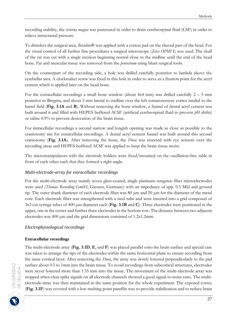
Methods
27
recording stability, the cisterna magna was punctured in order to drain cerebrospinal fluid (CSF) in order to
relieve intracranial pressure.
To disinfect the surgical area, Betadine® was applied with a cotton pad on the shaved part of the head. For
the visual control of all further fine procedures a surgical microscope (Zeiss OPMI I) was used. The skull
of the rat was cut with a single incision beginning nostral close to the midline until the end of the head
bone. Fat and muscular tissue was removed from the periosteum using blunt surgical tools.
On the counterpart of the recording side, a hole was drilled carefully posterior to lambda above the
cerebellar area. A clockmaker screw was fixed in this hole in order to serve as a fixation point for the acryl
cement which is applied later on the head bone.
For the extracellular recordings a small bone window (about 4x4 mm) was drilled carefully 2 – 3 mm
posterior to Bregma, and about 5 mm lateral to midline over the left somatosensory cortex medial to the
barrel field (Fig. 3.1A and B). Without removing the bone window, a funnel of dental acryl cement was
built around it and filled with HEPES buffered ACSF (artificial cerebrospinal fluid to prevent pH shifts)
or saline 0.9% to prevent desiccation of the brain tissue.
For intracellular recordings a second narrow and longish opening was made as close as possible to the
craniotomy site for extracellular recordings. A dental acryl cement funnel was built around this second
craniotomy (Fig. 3.1A). After removing the bone, the Dura was resected with eye scissors over the
recording areas and HEPES buffered ACSF was applied to keep the brain tissue moist.
The micromanipulators with the electrode holders were fixed/mounted on the oscillation-free table in
front of each other such that they formed a right angle.
Multi-electrode-array for extracellular recordings
For the multi-electrode array mainly seven glass-coated, single platinum–tungsten fiber microelectrodes
were used (Thomas Recording GmbH, Giessen, Germany) with an impedance of app. 0.5 MΩ and ground
tip. The outer shank diameter of each electrode fiber was 80 μm and 20 μm for the diameter of the metal
core. Each electrode fiber was strengthened with a steel tube and were inserted into a grid composed of
3x3 cut syringe tubes of 400 μm diameter each (Fig. 3.1B and C). Three electrodes were positioned in the
upper, one in the center and further three electrodes in the bottom row. The distance between two adjacent
electrodes was 400 μm and the grid dimensions consisted of 1.2x1.2mm.
Electrophysiological recordings
Extracellular recordings
The multi-electrode array (Fig. 3.1D, E, and F) was placed parallel onto the brain surface and special care
was taken to arrange the tips of the electrodes within the same horizontal plane to ensure recording from
the same cortical layer. After removing the Dura, the array was slowly lowered perpendicularly to the pial
surface about 0.5 to 1mm into the brain tissue. To avoid recordings from subcortical structures, electrodes
were never lowered more than 1.55 mm into the tissue. The movement of the multi-electrode array was
stopped when clear spike signals on all electrode channels showed a good signal-to-noise ratio. The multi-
electrode-array was then maintained in the same position for the whole experiment. The exposed cortex
(Fig. 3.1F) was covered with a low-melting-point paraffin wax to provide stabilization and to reduce brain
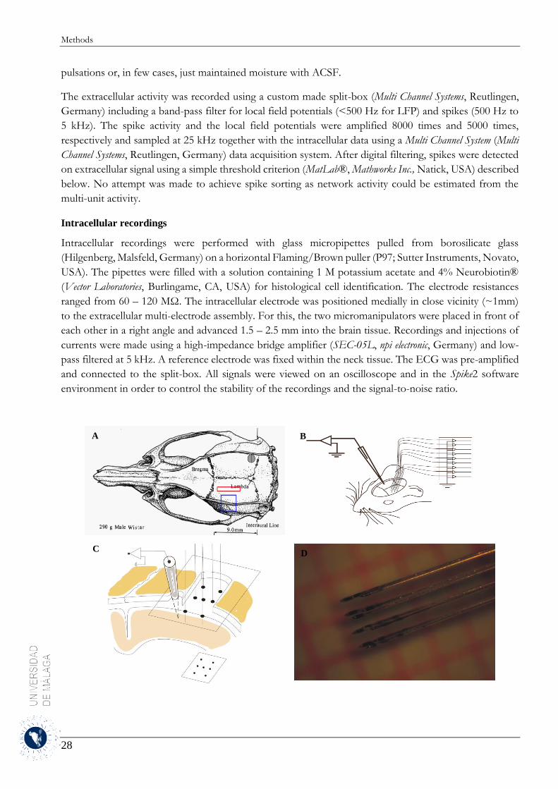
Methods
28
pulsations or, in few cases, just maintained moisture with ACSF.
The extracellular activity was recorded using a custom made split-box (Multi Channel Systems, Reutlingen,
Germany) including a band-pass filter for local field potentials (<500 Hz for LFP) and spikes (500 Hz to
5 kHz). The spike activity and the local field potentials were amplified 8000 times and 5000 times,
respectively and sampled at 25 kHz together with the intracellular data using a Multi Channel System (Multi
Channel Systems, Reutlingen, Germany) data acquisition system. After digital filtering, spikes were detected
on extracellular signal using a simple threshold criterion (MatLab®, Mathworks Inc., Natick, USA) described
below. No attempt was made to achieve spike sorting as network activity could be estimated from the
multi-unit activity.
Intracellular recordings
Intracellular recordings were performed with glass micropipettes pulled from borosilicate glass
(Hilgenberg, Malsfeld, Germany) on a horizontal Flaming/Brown puller (P97; Sutter Instruments, Novato,
USA). The pipettes were filled with a solution containing 1 M potassium acetate and 4% Neurobiotin®
(Vector Laboratories, Burlingame, CA, USA) for histological cell identification. The electrode resistances
ranged from 60 – 120 MΩ. The intracellular electrode was positioned medially in close vicinity (~1mm)
to the extracellular multi-electrode assembly. For this, the two micromanipulators were placed in front of
each other in a right angle and advanced 1.5 – 2.5 mm into the brain tissue. Recordings and injections of
currents were made using a high-impedance bridge amplifier (SEC-05L, npi electronic, Germany) and low-
pass filtered at 5 kHz. A reference electrode was fixed within the neck tissue. The ECG was pre-amplified
and connected to the split-box. All signals were viewed on an oscilloscope and in the Spike2 software
environment in order to control the stability of the recordings and the signal-to-noise ratio.
A
C D
B
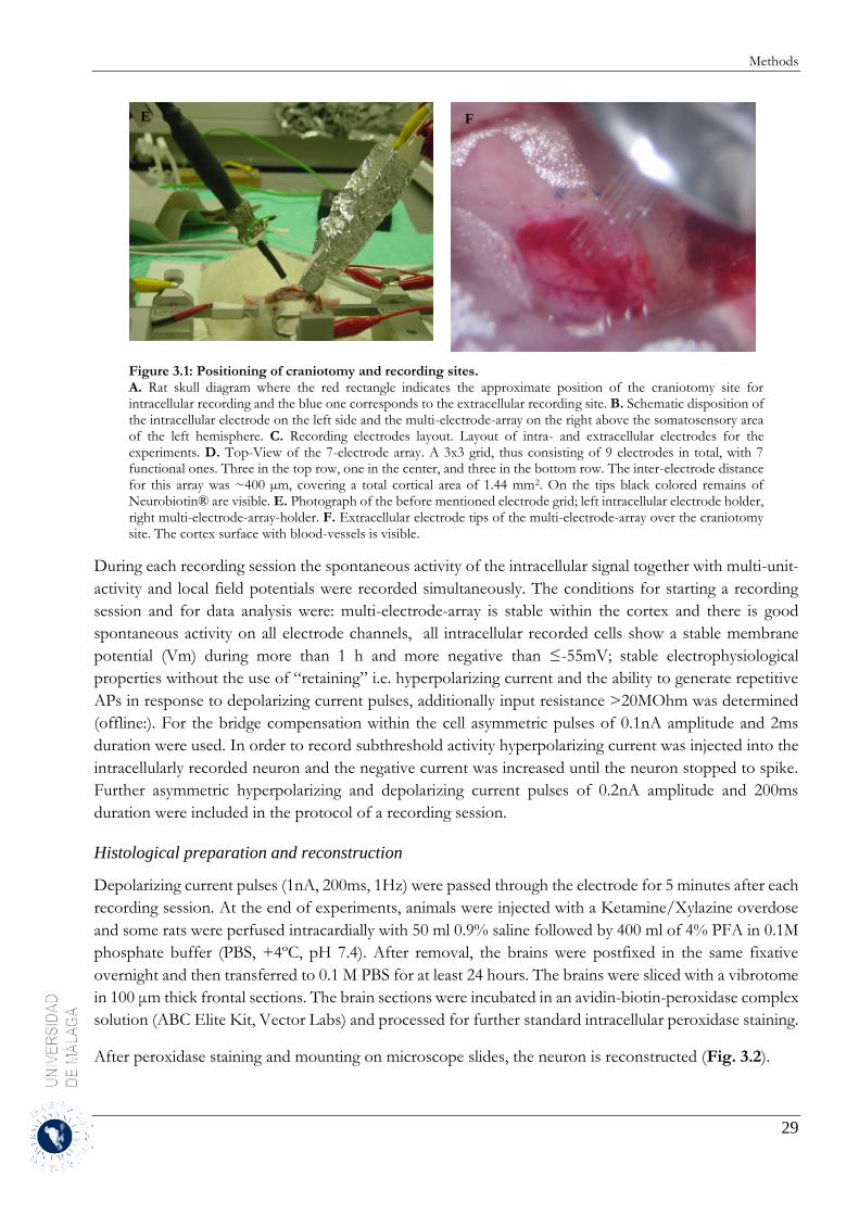
Methods
29
Figure 3.1: Positioning of craniotomy and recording sites. A. Rat skull diagram where the red rectangle indicates the approximate position of the craniotomy site for intracellular recording and the blue one corresponds to the extracellular recording site. B. Schematic disposition of the intracellular electrode on the left side and the multi-electrode-array on the right above the somatosensory area of the left hemisphere. C. Recording electrodes layout. Layout of intra- and extracellular electrodes for the experiments. D. Top-View of the 7-electrode array. A 3x3 grid, thus consisting of 9 electrodes in total, with 7 functional ones. Three in the top row, one in the center, and three in the bottom row. The inter-electrode distance for this array was ~400 µm, covering a total cortical area of 1.44 mm2. On the tips black colored remains of Neurobiotin® are visible. E. Photograph of the before mentioned electrode grid; left intracellular electrode holder, right multi-electrode-array-holder. F. Extracellular electrode tips of the multi-electrode-array over the craniotomy site. The cortex surface with blood-vessels is visible.
During each recording session the spontaneous activity of the intracellular signal together with multi-unit-
activity and local field potentials were recorded simultaneously. The conditions for starting a recording
session and for data analysis were: multi-electrode-array is stable within the cortex and there is good
spontaneous activity on all electrode channels, all intracellular recorded cells show a stable membrane
potential (Vm) during more than 1 h and more negative than ≤-55mV; stable electrophysiological
properties without the use of “retaining” i.e. hyperpolarizing current and the ability to generate repetitive
APs in response to depolarizing current pulses, additionally input resistance >20MOhm was determined
(offline:). For the bridge compensation within the cell asymmetric pulses of 0.1nA amplitude and 2ms
duration were used. In order to record subthreshold activity hyperpolarizing current was injected into the
intracellularly recorded neuron and the negative current was increased until the neuron stopped to spike.
Further asymmetric hyperpolarizing and depolarizing current pulses of 0.2nA amplitude and 200ms
duration were included in the protocol of a recording session.
Histological preparation and reconstruction
Depolarizing current pulses (1nA, 200ms, 1Hz) were passed through the electrode for 5 minutes after each
recording session. At the end of experiments, animals were injected with a Ketamine/Xylazine overdose
and some rats were perfused intracardially with 50 ml 0.9% saline followed by 400 ml of 4% PFA in 0.1M
phosphate buffer (PBS, +4ºC, pH 7.4). After removal, the brains were postfixed in the same fixative
overnight and then transferred to 0.1 M PBS for at least 24 hours. The brains were sliced with a vibrotome
in 100 μm thick frontal sections. The brain sections were incubated in an avidin-biotin-peroxidase complex
solution (ABC Elite Kit, Vector Labs) and processed for further standard intracellular peroxidase staining.
After peroxidase staining and mounting on microscope slides, the neuron is reconstructed (Fig. 3.2).
E F
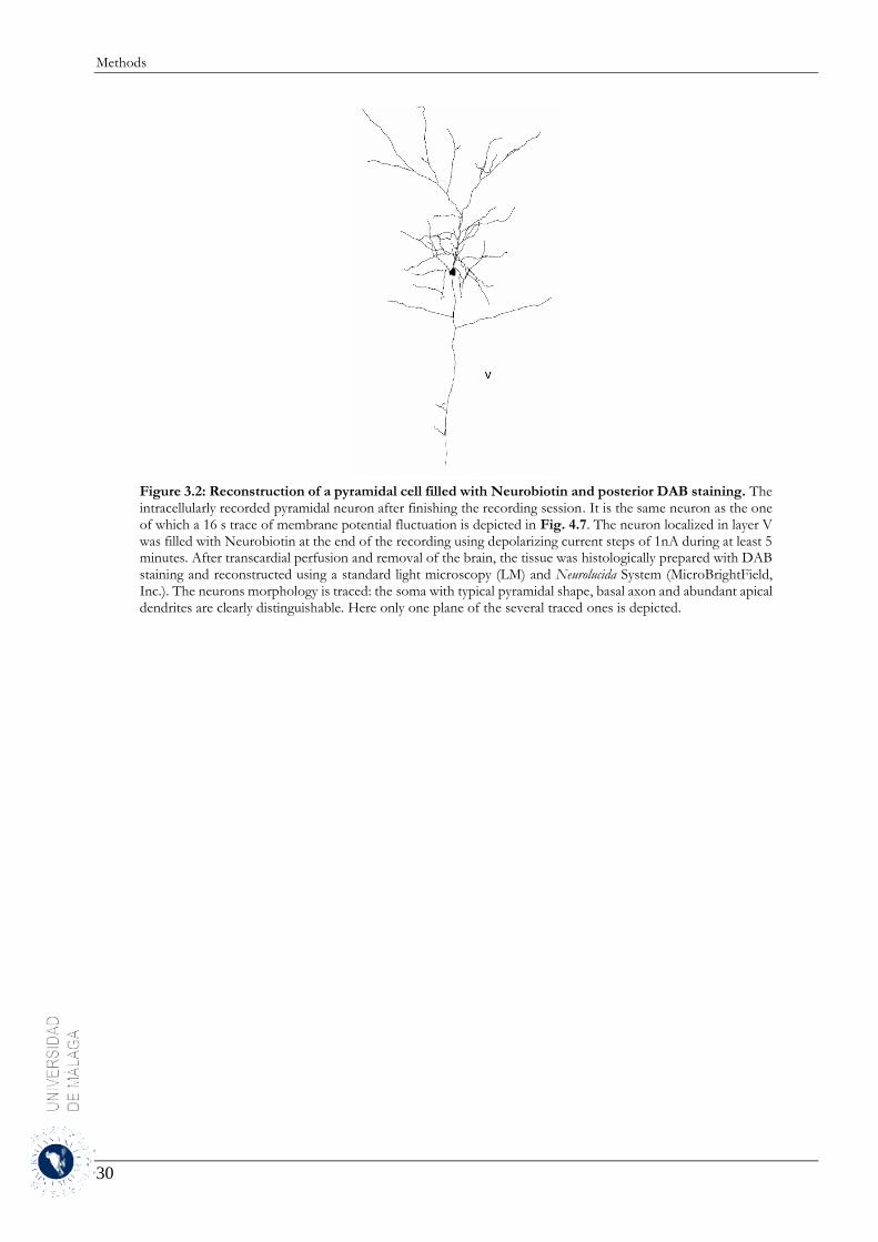
Methods
30
Figure 3.2: Reconstruction of a pyramidal cell filled with Neurobiotin and posterior DAB staining. The intracellularly recorded pyramidal neuron after finishing the recording session. It is the same neuron as the one of which a 16 s trace of membrane potential fluctuation is depicted in Fig. 4.7. The neuron localized in layer V was filled with Neurobiotin at the end of the recording using depolarizing current steps of 1nA during at least 5 minutes. After transcardial perfusion and removal of the brain, the tissue was histologically prepared with DAB staining and reconstructed using a standard light microscopy (LM) and Neurolucida System (MicroBrightField, Inc.). The neurons morphology is traced: the soma with typical pyramidal shape, basal axon and abundant apical dendrites are clearly distinguishable. Here only one plane of the several traced ones is depicted.
Results
31
4 Results
4.1 Up and Down states identification using moving averages
Up and Down states were identified in intracellular recordings obtained from the cerebral
cortex of both in vitro and in vivo preparations from different areas of the cortex (visual,
prefrontal and somatosensory). In the first part of the results we describe the properties of
MAUDS analyzing the recordings with the MATLAB® scripts in an offline fashion. In the
second part of the results we demonstrate how this method can also be used online, thus
being useful to exploit the signals that it generates to trigger other events or to obtain
immediate statistics of time distribution of Up versus Down states under different conditions.
4.1.1 Properties of MAUDS analyzing the Up and Down states
The characteristic shape of neuronal membrane potential during slow oscillations shows two
clearly differentiated states of membrane potential: a depolarized membrane (Up states) and
a hyperpolarized one (Down states), with relatively fast transitions between them. As said
before, in short recordings, Up and Down states are often identified by thresholding the
membrane potential. However, this method frequently fails in long recordings due to
membrane potential drifting, presence of spindles, and other types of interferences like
electronic noise or movement artefacts while in vivo (heartbeat pulsation, respiratory
movements, etc). Even when the aim of the experimentalists should be to eliminate all these
artefacts, we will exploit them here in order to test the robustness of the described method
against others commonly used.
Two problems have to be solved for a good characterization of the states: (1) determining
the periods where depolarized (Up state) or hyperpolarized (Down state) membrane
potential take place, and (2) identifying the precise points in time where these states actually
start and end. As explained in the methods section, MAUDS tackles these problems with
an initial broad identification of the Down states by over-crossing two moving averages, and
a later refinement of the initiation and termination points by a discrete processing of the
membrane potential evolution in the transition interval. In general, we have observed that
MAUDS performs well for any value of the long-term EMA in a wide range. On the other
hand, the characterization is slightly more sensitive to the fast EMA. An optimum window
size would smooth efficiently the high frequency changes of the membrane potential
(isolated spikes and artefacts), being also quick enough to detect fast excursions of the signal
to highly hyperpolarized regions.
We studied periods of 900 seconds of intracellular fluctuations in recordings from neurons
in the visual cortex of the anesthetized cat, from neurons in the somatosensorial cortex in
the anesthetized rat, and from neurons recorded in oscillating ferret cortical slices obtained
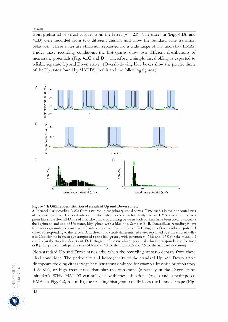
Results
32
from prefrontal or visual cortices from the ferret (n = 20). The traces in (Fig. 4.1A, and
4.1B) were recorded from two different animals and show the standard state transition
behavior. These states are efficiently separated for a wide range of fast and slow EMAs.
Under these recording conditions, the histograms show two different distributions of
membrane potentials (Fig. 4.1C and D). Therefore, a simple thresholding is expected to
reliably separate Up and Down states. (Overshadowing blue boxes show the precise limits
of the Up states found by MAUDS, in this and the following figures.)
Figure 4.1: Offline identification of standard Up and Down states. A. Intracellular recording in vivo from a neuron in cat primary visual cortex. Time marks in the horizontal axes of the traces indicate 1 second interval (relative labels not shown for clarity). A fast EMA is represented as a green line and a slow EMA in red line. The points of crossing between both of them have been used to calculate the beginning and end of Up states, highlighted with a blue box. Same in B. B. Intracellular recording in vitro from a supragranular neuron in a prefrontal cortex slice from the ferret. C. Histogram of the membrane potential values corresponding to the trace in A. It shows two clearly differentiated states separated by a transitional valley (see Gaussian fit in green superimposed to the histograms, with parameters -76.6 and -67.0 for the mean, 0.8 and 5.3 for the standard deviation). D. Histogram of the membrane potential values corresponding to the trace in B (fitting curves with parameters -64.6 and -57.0 for the mean, 0.5 and 7.6 for the standard deviation).
Non-standard Up and Down states arise when the recording scenario departs from these
ideal conditions. The periodicity and homogeneity of the standard Up and Down states
disappears, yielding either irregular fluctuations (induced for example by noise or respiratory
if in vivo), or high frequencies that blur the transitions (especially in the Down states
initiation). While MAUDS can still deal with these situations (traces and superimposed
EMAs in Fig. 4.2, A and B), the resulting histogram rapidly loses the bimodal shape (Fig.

Results
33
4.2C and D), making it harder to decide where the right threshold should be located. Since
the duration of Up and Down states presents a large variability, it is also difficult to filter
false transitions according to this feature. The histograms performed over longer recording
sessions simply showed a smoothed shape, but failed to better define the two-peaks picture.
Another undesired artefact is signal drifting, caused by changes in the junction potential. In
principle this effect can be prevented (chloriding silver electrodes, using an agar bridge, etc.)
and compensated by commercial amplifiers, but it is usual to obtain long sequences of data
where slow shifts (e.g. Fig, 4.2A) or fast excursions of the membrane potentials can be
observed. These variations in the apparent membrane potential do not necessarily reflect
any change in the current flowing through the membrane but an offset of the membrane
potential value. Therefore, the bistable fluctuation of the membrane potential during
rhythmic activity remains, allowing it to be studied in spite of the unstable wave it is resting
on (Fig. 4.2).
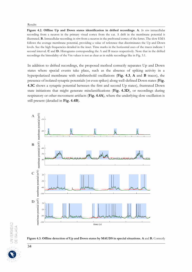
Results
34
Figure 4.2. Offline Up and Down states identification in drifted recordings. A. In vivo intracellular
recording from a neuron in the primary visual cortex from the cat. A drift in the membrane potential is
illustrated. B. Intracellular recording in vitro from a neuron in the prefrontal cortex of the ferret. The slow EMA
follows the average membrane potential, providing a value of reference that discriminates the Up and Down
levels. See the high frequencies detailed in the inset. Time marks in the horizontal axes of the traces indicate 1
second interval. C and D. Histograms corresponding the A and B traces respectively. Note that in the drifted
recordings the bimodality of the Vm values is not as clear as in stable recordings like in Fig. 3.1.
In addition to drifted recordings, the proposed method correctly separates Up and Down
states where special events take place, such as the absence of spiking activity in a
hyperpolarized membrane with subthreshold oscillations (Fig. 4.3, A and B traces), the
presence of isolated synaptic potentials (or even spikes) along well-defined Down states (Fig.
4.3C shows a synaptic potential between the first and second Up states), frustrated Down
state initiations that might generate misclassifications (Fig. 4.3D), or recordings during
respiratory or other movement artifacts (Fig. 4.4A), where the underlying slow oscillation is
still present (detailed in Fig. 4.4B).
Figure 4.3. Offline detection of Up and Down states by MAUDS in special situations. A and B. Correctly

Results
35
identifying Up states where no action potentials occur in highly hyperpolarized neurons recorded in vitro in prefrontal cortex from the ferret. Note that in B there is correct detection of Down states in spite of the repetitive occurrence of short lasting sharp events. C. Filtering isolated synaptic events occurring in the middle of a Down state. D. Sorting suspicious Down states intermingled into long-lasting Up states (third Up state). C and D correspond to intracellular recordings obtained in vivo from cat’s primary visual cortex. In all panels time marks in the horizontal axes of the traces indicate 1 second interval.
The histograms of membrane potential show that some bimodal distribution remains (Fig.
4.4D) over stable intervals, but it vanishes when applied to a few seconds interval (Fig. 4.4C
shows the histogram for the trace on Fig. 4.4A).
Figure 4.4. Offline identification of Up and Down states in intracellular recordings with artifacts. A. Intracellular recording from primary visual cortex of the cat in vivo. There is a respiratory movement artifact that generates rhythmic drifts of the membrane potential. B. Detail of a portion of the membrane potential shown in A (second 15, 16, 17). Time marks in the horizontal axes of the traces indicate 1 second interval. C and D. The distributions of membrane potentials in panels A and B, respectively.
In order to compare the performance of MAUDS with that of the histogram method, 5
recordings containing standard slow oscillation were selected (for an overall time of 145 s)
and the corresponding transitions were obtained based on the histogram (best manual fitting)
and with MAUDS, where a broad estimation of the oscillation frequency parameterized the
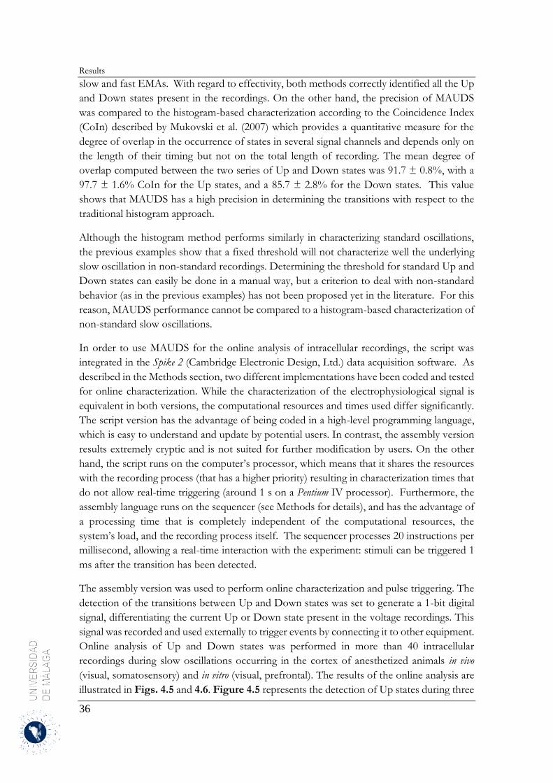
Results
36
slow and fast EMAs. With regard to effectivity, both methods correctly identified all the Up
and Down states present in the recordings. On the other hand, the precision of MAUDS
was compared to the histogram-based characterization according to the Coincidence Index
(CoIn) described by Mukovski et al. (2007) which provides a quantitative measure for the
degree of overlap in the occurrence of states in several signal channels and depends only on
the length of their timing but not on the total length of recording. The mean degree of
overlap computed between the two series of Up and Down states was 91.7 ± 0.8%, with a
97.7 ± 1.6% CoIn for the Up states, and a 85.7 ± 2.8% for the Down states. This value
shows that MAUDS has a high precision in determining the transitions with respect to the
traditional histogram approach.
Although the histogram method performs similarly in characterizing standard oscillations,
the previous examples show that a fixed threshold will not characterize well the underlying
slow oscillation in non-standard recordings. Determining the threshold for standard Up and
Down states can easily be done in a manual way, but a criterion to deal with non-standard
behavior (as in the previous examples) has not been proposed yet in the literature. For this
reason, MAUDS performance cannot be compared to a histogram-based characterization of
non-standard slow oscillations.
In order to use MAUDS for the online analysis of intracellular recordings, the script was
integrated in the Spike 2 (Cambridge Electronic Design, Ltd.) data acquisition software. As
described in the Methods section, two different implementations have been coded and tested
for online characterization. While the characterization of the electrophysiological signal is
equivalent in both versions, the computational resources and times used differ significantly.
The script version has the advantage of being coded in a high-level programming language,
which is easy to understand and update by potential users. In contrast, the assembly version
results extremely cryptic and is not suited for further modification by users. On the other
hand, the script runs on the computer’s processor, which means that it shares the resources
with the recording process (that has a higher priority) resulting in characterization times that
do not allow real-time triggering (around 1 s on a Pentium IV processor). Furthermore, the
assembly language runs on the sequencer (see Methods for details), and has the advantage of
a processing time that is completely independent of the computational resources, the
system’s load, and the recording process itself. The sequencer processes 20 instructions per
millisecond, allowing a real-time interaction with the experiment: stimuli can be triggered 1
ms after the transition has been detected.
The assembly version was used to perform online characterization and pulse triggering. The
detection of the transitions between Up and Down states was set to generate a 1-bit digital
signal, differentiating the current Up or Down state present in the voltage recordings. This
signal was recorded and used externally to trigger events by connecting it to other equipment.
Online analysis of Up and Down states was performed in more than 40 intracellular
recordings during slow oscillations occurring in the cortex of anesthetized animals in vivo
(visual, somatosensory) and in vitro (visual, prefrontal). The results of the online analysis are
illustrated in Figs. 4.5 and 4.6. Figure 4.5 represents the detection of Up states during three
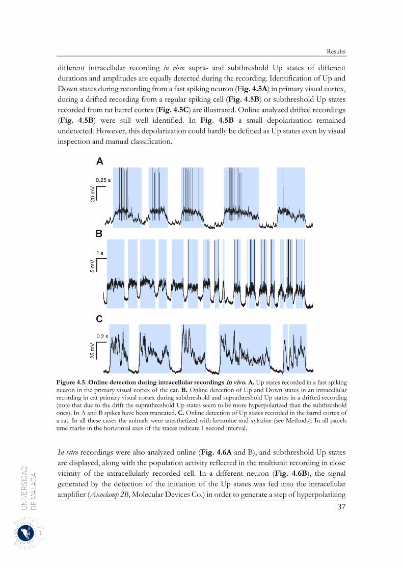
Results
37
different intracellular recording in vivo: supra- and subthreshold Up states of different
durations and amplitudes are equally detected during the recording. Identification of Up and
Down states during recording from a fast spiking neuron (Fig. 4.5A) in primary visual cortex,
during a drifted recording from a regular spiking cell (Fig. 4.5B) or subthreshold Up states
recorded from rat barrel cortex (Fig. 4.5C) are illustrated. Online analyzed drifted recordings
(Fig. 4.5B) were still well identified. In Fig. 4.5B a small depolarization remained
undetected. However, this depolarization could hardly be defined as Up states even by visual
inspection and manual classification.
Figure 4.5. Online detection during intracellular recordings in vivo. A. Up states recorded in a fast spiking neuron in the primary visual cortex of the cat. B. Online detection of Up and Down states in an intracellular recording in cat primary visual cortex during subthreshold and suprathreshold Up states in a drifted recording (note that due to the drift the suprathreshold Up states seem to be more hyperpolarized than the subthreshold ones). In A and B spikes have been truncated. C. Online detection of Up states recorded in the barrel cortex of a rat. In all these cases the animals were anesthetized with ketamine and xylazine (see Methods). In all panels time marks in the horizontal axes of the traces indicate 1 second interval.
In vitro recordings were also analyzed online (Fig. 4.6A and B), and subthreshold Up states
are displayed, along with the population activity reflected in the multiunit recording in close
vicinity of the intracellularly recorded cell. In a different neuron (Fig. 4.6B), the signal
generated by the detection of the initiation of the Up states was fed into the intracellular
amplifier (Axoclamp 2B, Molecular Devices Co.) in order to generate a step of hyperpolarizing
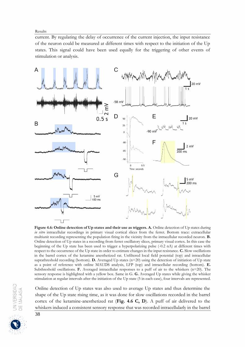
Results
38
current. By regulating the delay of occurrence of the current injection, the input resistance
of the neuron could be measured at different times with respect to the initiation of the Up
states. This signal could have been used equally for the triggering of other events of
stimulation or analysis.
Figure 4.6: Online detection of Up states and their use as triggers. A. Online detection of Up states during in vitro intracellular recordings in primary visual cortical slices from the ferret. Bottom trace: extracellular multiunit recording representing the population firing in the vicinity from the intracellular recorded neuron. B. Online detection of Up states in a recording from ferret oscillatory slices, primary visual cortex. In this case the beginning of the Up state has been used to trigger a hyperpolarizing pulse (-0.2 nA) at different times with respect to the occurrence of the Up state in order to estimate changes in the input resistance. C. Slow oscillations in the barrel cortex of the ketamine anesthetized rat. Unfiltered local field potential (top) and intracellular suprathreshold recording (bottom). D. Averaged Up states (n=20) using the detection of initiation of Up state as a point of reference with online MAUDS analysis, LFP (top) and intracellular recording (bottom). E. Subthreshold oscillations. F. Averaged intracellular responses to a puff of air to the whiskers (n=20). The sensory response is highlighted with a yellow box. Same in G. G. Averaged Up states while giving the whisker stimulation at regular intervals after the initiation of the Up state (5 in each case), four intervals are represented.
Online detection of Up states was also used to average Up states and thus determine the
shape of the Up state rising time, as it was done for slow oscillations recorded in the barrel
cortex of the ketamine-anesthetized rat (Fig. 4.6 C, D). A puff of air delivered to the
whiskers induced a consistent sensory response that was recorded intracellularly in the barrel

Results
39
cortex (Fig. 4.6F). The signal generated by the online detection of the Up states’ initiation
was also used to trigger the sensory responses at particular intervals after the initiation of the
Up states, thus allowing systematic average of different trials (Fig. 3.6G).
Results
40
4.2 Spatiotemporal structure of spontaneous slow-wave oscillations in
the neocortex
By combining seven extracellular recordings with one simultaneous intracellular recording,
we investigated the spatio-temporal structure of slow-wave activity in vivo in the rat
somatosensorial neocortex under ketamine/xylazine anesthesia.
To monitor the spatio-temporal pattern of cortical state-transitions in a tangential plane, a
planar array of 7 extracellular electrodes distributed on a 3x3 grid, as shown in Fig. 3.2A and
Fig. 3.2C, was used including differential filtering for multi-unit-activity (MUA) and local
field potential (LFP) signals (Fig. 4.7). All electrodes were protruded together into the
somatosensory cortex medial to the barrel field (Fig. 3.2A, B and C). Recording depth was
less than 1.5 mm. After successful positioning of the extracellular electrode array, a stable
intracellular recording in the vicinity of the array (distance of <1 mm) was established. The
intracellular recording was used as a point of reference to detect the state transitions of the
slow-wave oscillations based on synaptic activity. Triggered on these state transitions,
multiple episodes of spike activity were extracted from the extracellular electrodes and the
state transition was determined for each of the individual electrodes from the averaged
episodes. The emerging spatiotemporal pattern was then tested for pattern consistency and
variability across repeated activity waves employing single trial rate estimates.
While in the previous section (section 4.1) the MAUDS method was described and discussed,
in this section the common histogram based analysis was performed in order to study the
spatio-temporal structure of spontaneous slow-wave oscillation. Furthermore, the data
analysis of the recordings involving the 7-electrode array (3 x 3 grid), positioned parallel to
the pial surface, is detailed.
4.2.1 Down-to-Up transition
During a recording session, as described previously in the Methods section data was recorded
only when several conditions were met. First, at least 5 out of the 7 electrodes in the array
had to show some type of multi-unit activity. Second, the membrane potential of the
intracellular electrode had to be stable and hyperpolarized to at least - 65 mV. Recording
times ranged between 90-620 seconds depending on the stability of the intracellular
membrane potential. Prior to starting the actual data analysis, the raw data was carefully
looked over to pre-select which data had the desired characteristics. These included clear Up
and Down states in the intracellular data, increased multi-unit activity in the extracellular data
approximately coinciding with the Up state in the intracellular recording, good signal to noise
ratio and no artifacts such as 50 Hz noise. See Fig. 4.1 for examples of raw data that full-
filled these requirements. Five intracellular recordings from 4 rats were included in the
analysis.
Results
41
As previously mentioned, the anesthetics urethane in combination with ketamine/xylazine
leads to fluctuations in membrane potential, namely Up and Down states. The first part of
the analysis involved the detection of both the onset and offset of these two states, which
can be carried out using different techniques as previously mentioned. One proposed
technique uses the spectral differences in recorded local field potentials (LFPs) during active
and silent states for their detection method (Mukovski et al., 2007). Given that LFPs are
lowpass filtered extracellular recordings, this would justify the use of extracellular MUA for
the extraction of state transitions, a principle we made use of in our later analysis. Other
techniques for the identification of active and silent states required the use of simultaneously
recorded electroencephalogram (EEG) or electrocorticogram (ECoG) (Waters and
Helmchen, 2006).
Two additional methods, based on the simultaneous intracellular recording, can be
performed in two slightly different ways. In the first method, a three-dimensional plot was
constructed consisting of the mean and standard deviation determined for a 50 ms running
window. As seen in Fig. 4.8, the Down states are represented by a sharp peak at
hyperpolarized membrane potentials (~-69 mV) and very small standard deviations (~0.6).
The Up state on the other hand is not as clearly discernable, only a broader peak centered at
a membrane potential of about -58 mV and a standard deviation of about 6.3 give hints on
the position of the Up state. The pseudocolor plot underneath the histogram is a slightly
better depiction of the two states. Here, the Up state region is outlined in red and the Down
state region in orange.
A second method for the identification of the two states is to plot the membrane potential
distributions and by the resulting bimodality of the plot, which is due to the presence of the
membrane fluctuations, the two states can be separated. The Fig. 4.9B shows the bimodal
distribution of a 20 s intracellular data recording. The peak located at more hyperpolarized
levels represents the Down states, whereas the somewhat broader, smaller amplitude peak
represents the Up states. Not in all cases were the peaks this clearly separable. Occasionally
the smaller peak was absent and an approximation had to be made regarding its location.
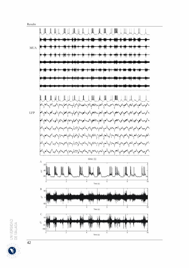
Results
42
MUA
LFP
time (s)
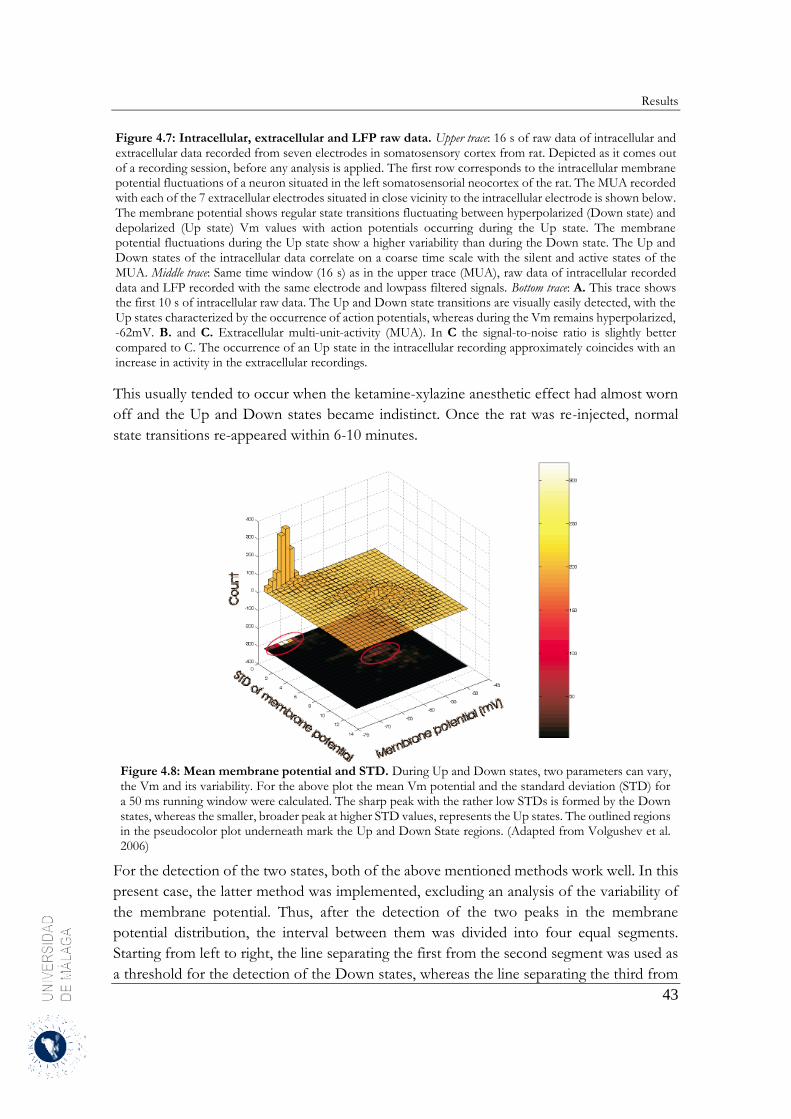
Results
43
Figure 4.7: Intracellular, extracellular and LFP raw data. Upper trace: 16 s of raw data of intracellular and extracellular data recorded from seven electrodes in somatosensory cortex from rat. Depicted as it comes out of a recording session, before any analysis is applied. The first row corresponds to the intracellular membrane potential fluctuations of a neuron situated in the left somatosensorial neocortex of the rat. The MUA recorded with each of the 7 extracellular electrodes situated in close vicinity to the intracellular electrode is shown below. The membrane potential shows regular state transitions fluctuating between hyperpolarized (Down state) and depolarized (Up state) Vm values with action potentials occurring during the Up state. The membrane potential fluctuations during the Up state show a higher variability than during the Down state. The Up and Down states of the intracellular data correlate on a coarse time scale with the silent and active states of the MUA. Middle trace: Same time window (16 s) as in the upper trace (MUA), raw data of intracellular recorded data and LFP recorded with the same electrode and lowpass filtered signals. Bottom trace: A. This trace shows the first 10 s of intracellular raw data. The Up and Down state transitions are visually easily detected, with the Up states characterized by the occurrence of action potentials, whereas during the Vm remains hyperpolarized, -62mV. B. and C. Extracellular multi-unit-activity (MUA). In C the signal-to-noise ratio is slightly better compared to C. The occurrence of an Up state in the intracellular recording approximately coincides with an increase in activity in the extracellular recordings.
This usually tended to occur when the ketamine-xylazine anesthetic effect had almost worn
off and the Up and Down states became indistinct. Once the rat was re-injected, normal
state transitions re-appeared within 6-10 minutes.
Figure 4.8: Mean membrane potential and STD. During Up and Down states, two parameters can vary, the Vm and its variability. For the above plot the mean Vm potential and the standard deviation (STD) for a 50 ms running window were calculated. The sharp peak with the rather low STDs is formed by the Down states, whereas the smaller, broader peak at higher STD values, represents the Up states. The outlined regions in the pseudocolor plot underneath mark the Up and Down State regions. (Adapted from Volgushev et al. 2006)
For the detection of the two states, both of the above mentioned methods work well. In this
present case, the latter method was implemented, excluding an analysis of the variability of
the membrane potential. Thus, after the detection of the two peaks in the membrane
potential distribution, the interval between them was divided into four equal segments.
Starting from left to right, the line separating the first from the second segment was used as
a threshold for the detection of the Down states, whereas the line separating the third from
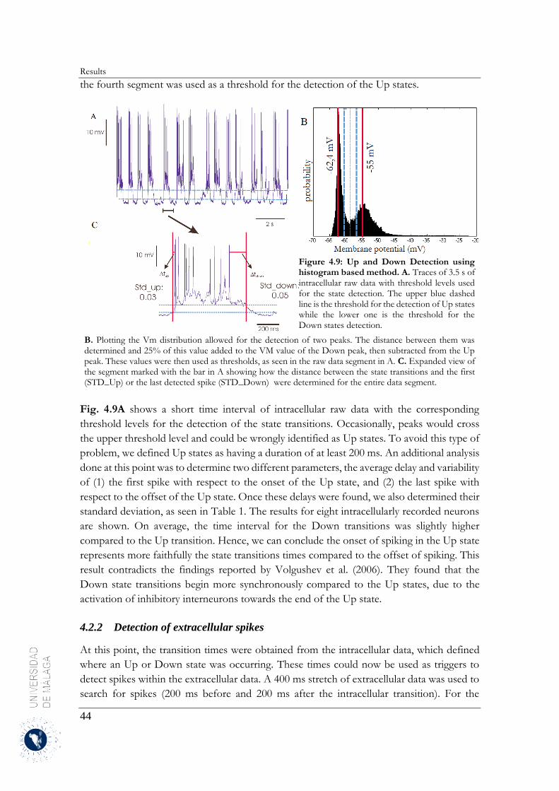
Results
44
the fourth segment was used as a threshold for the detection of the Up states.
Figure 4.9: Up and Down Detection using histogram based method. A. Traces of 3.5 s of intracellular raw data with threshold levels used for the state detection. The upper blue dashed line is the threshold for the detection of Up states while the lower one is the threshold for the Down states detection.
B. Plotting the Vm distribution allowed for the detection of two peaks. The distance between them was determined and 25% of this value added to the VM value of the Down peak, then subtracted from the Up peak. These values were then used as thresholds, as seen in the raw data segment in A. C. Expanded view of the segment marked with the bar in A showing how the distance between the state transitions and the first (STD_Up) or the last detected spike (STD_Down) were determined for the entire data segment.
Fig. 4.9A shows a short time interval of intracellular raw data with the corresponding
threshold levels for the detection of the state transitions. Occasionally, peaks would cross
the upper threshold level and could be wrongly identified as Up states. To avoid this type of
problem, we defined Up states as having a duration of at least 200 ms. An additional analysis
done at this point was to determine two different parameters, the average delay and variability
of (1) the first spike with respect to the onset of the Up state, and (2) the last spike with
respect to the offset of the Up state. Once these delays were found, we also determined their
standard deviation, as seen in Table 1. The results for eight intracellularly recorded neurons
are shown. On average, the time interval for the Down transitions was slightly higher
compared to the Up transition. Hence, we can conclude the onset of spiking in the Up state
represents more faithfully the state transitions times compared to the offset of spiking. This
result contradicts the findings reported by Volgushev et al. (2006). They found that the
Down state transitions begin more synchronously compared to the Up states, due to the
activation of inhibitory interneurons towards the end of the Up state.
4.2.2 Detection of extracellular spikes
At this point, the transition times were obtained from the intracellular data, which defined
where an Up or Down state was occurring. These times could now be used as triggers to
detect spikes within the extracellular data. A 400 ms stretch of extracellular data was used to
search for spikes (200 ms before and 200 ms after the intracellular transition). For the
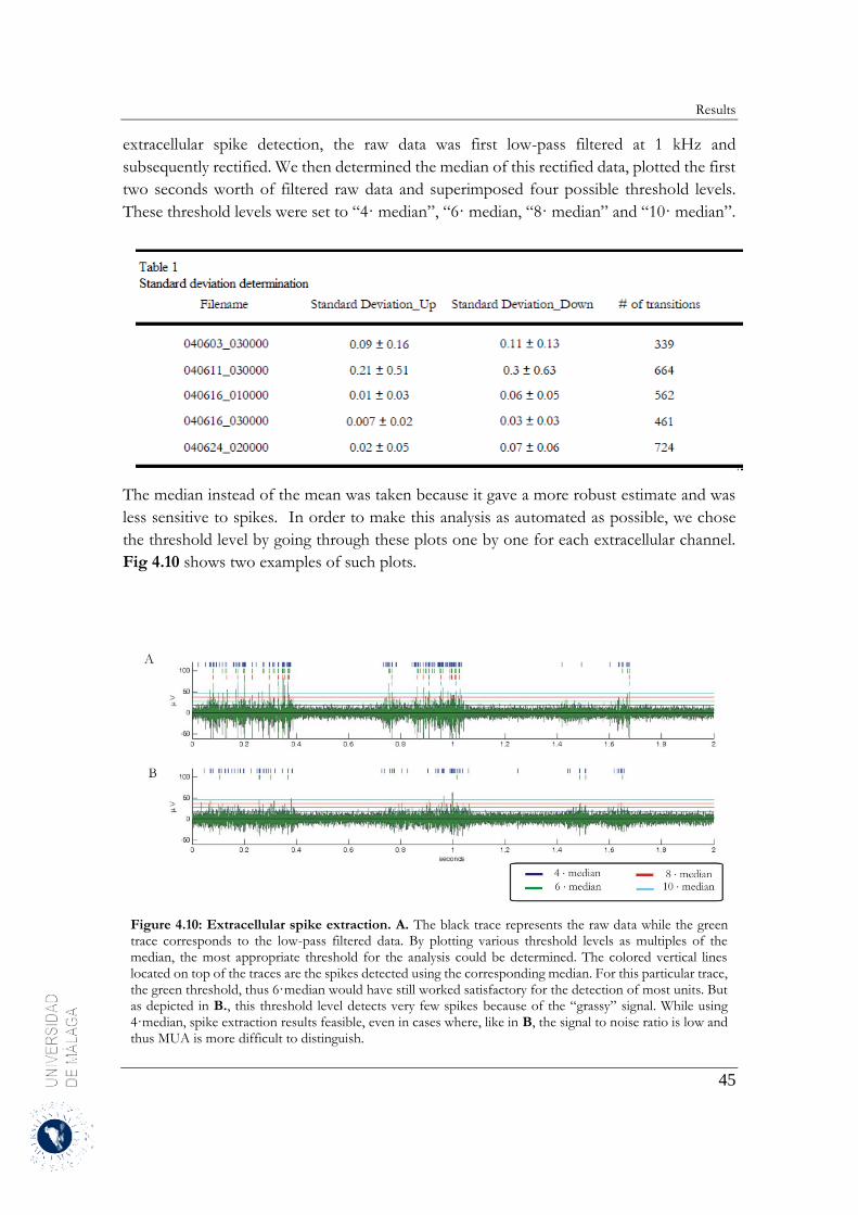
Results
45
extracellular spike detection, the raw data was first low-pass filtered at 1 kHz and
subsequently rectified. We then determined the median of this rectified data, plotted the first
two seconds worth of filtered raw data and superimposed four possible threshold levels.
These threshold levels were set to “4· median”, “6· median, “8· median” and “10· median”.
The median instead of the mean was taken because it gave a more robust estimate and was
less sensitive to spikes. In order to make this analysis as automated as possible, we chose
the threshold level by going through these plots one by one for each extracellular channel.
Fig 4.10 shows two examples of such plots.
Figure 4.10: Extracellular spike extraction. A. The black trace represents the raw data while the green trace corresponds to the low-pass filtered data. By plotting various threshold levels as multiples of the median, the most appropriate threshold for the analysis could be determined. The colored vertical lines located on top of the traces are the spikes detected using the corresponding median. For this particular trace, the green threshold, thus 6·median would have still worked satisfactory for the detection of most units. But as depicted in B., this threshold level detects very few spikes because of the “grassy” signal. While using 4·median, spike extraction results feasible, even in cases where, like in B, the signal to noise ratio is low and thus MUA is more difficult to distinguish.
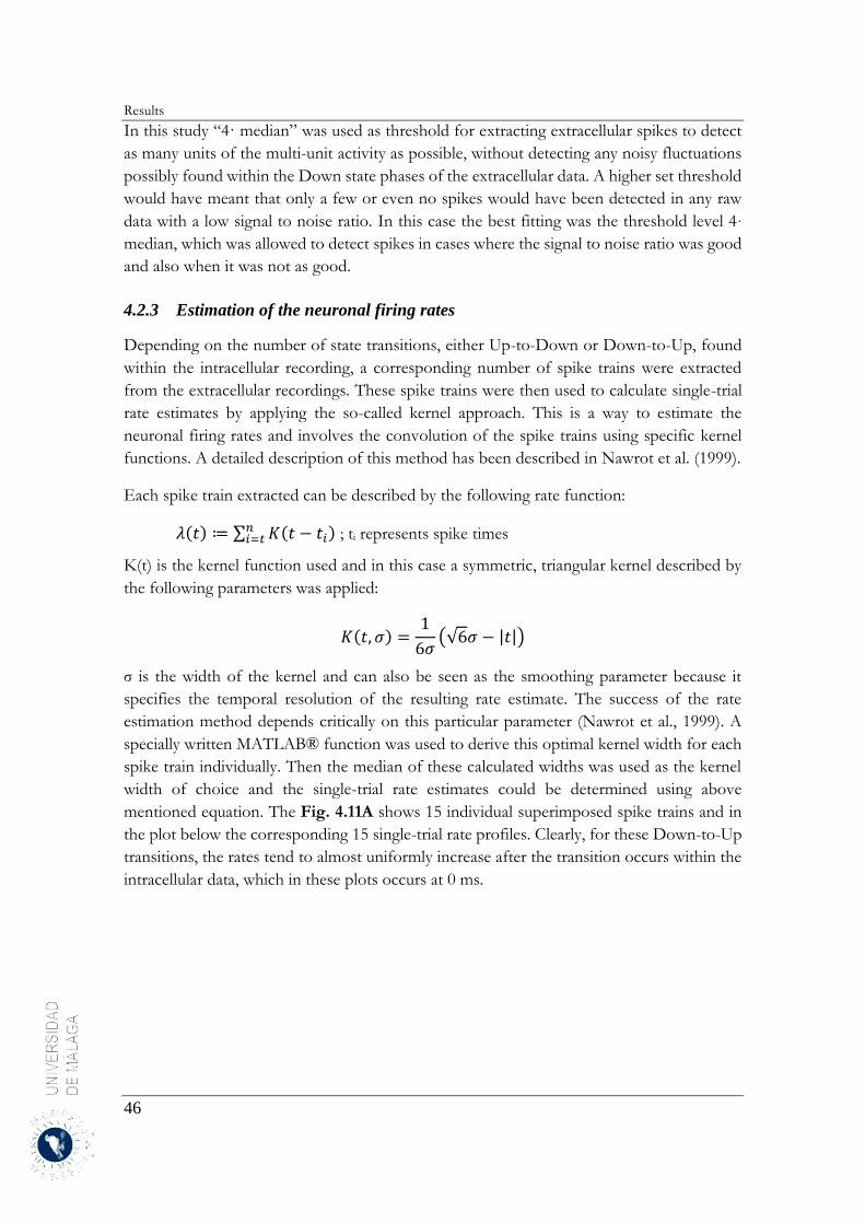
Results
46
In this study “4· median” was used as threshold for extracting extracellular spikes to detect
as many units of the multi-unit activity as possible, without detecting any noisy fluctuations
possibly found within the Down state phases of the extracellular data. A higher set threshold
would have meant that only a few or even no spikes would have been detected in any raw
data with a low signal to noise ratio. In this case the best fitting was the threshold level 4·
median, which was allowed to detect spikes in cases where the signal to noise ratio was good
and also when it was not as good.
4.2.3 Estimation of the neuronal firing rates
Depending on the number of state transitions, either Up-to-Down or Down-to-Up, found
within the intracellular recording, a corresponding number of spike trains were extracted
from the extracellular recordings. These spike trains were then used to calculate single-trial
rate estimates by applying the so-called kernel approach. This is a way to estimate the
neuronal firing rates and involves the convolution of the spike trains using specific kernel
functions. A detailed description of this method has been described in Nawrot et al. (1999).
Each spike train extracted can be described by the following rate function:
𝜆(𝑡) ≔ ∑ 𝐾(𝑡 − 𝑡𝑖)𝑛𝑖=𝑡 ; ti represents spike times
K(t) is the kernel function used and in this case a symmetric, triangular kernel described by
the following parameters was applied:
𝐾(𝑡, 𝜎) =1
6𝜎(√6𝜎 − |𝑡|)
σ is the width of the kernel and can also be seen as the smoothing parameter because it
specifies the temporal resolution of the resulting rate estimate. The success of the rate
estimation method depends critically on this particular parameter (Nawrot et al., 1999). A
specially written MATLAB® function was used to derive this optimal kernel width for each
spike train individually. Then the median of these calculated widths was used as the kernel
width of choice and the single-trial rate estimates could be determined using above
mentioned equation. The Fig. 4.11A shows 15 individual superimposed spike trains and in
the plot below the corresponding 15 single-trial rate profiles. Clearly, for these Down-to-Up
transitions, the rates tend to almost uniformly increase after the transition occurs within the
intracellular data, which in these plots occurs at 0 ms.
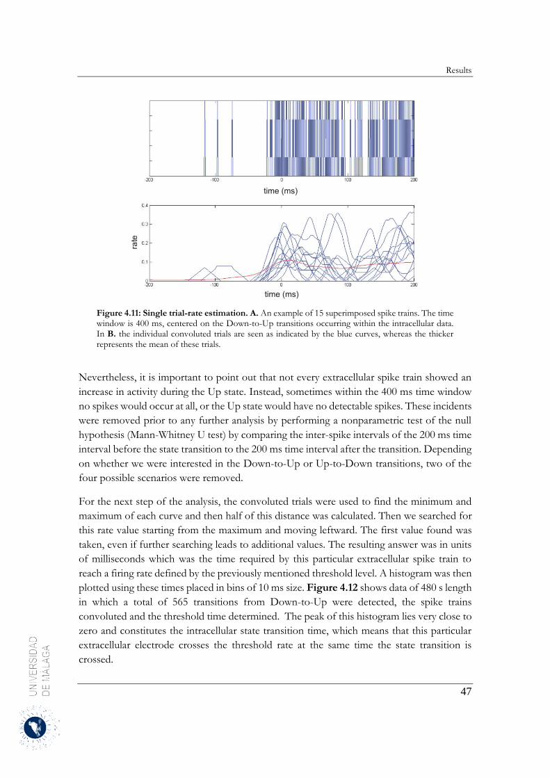
Results
47
Figure 4.11: Single trial-rate estimation. A. An example of 15 superimposed spike trains. The time window is 400 ms, centered on the Down-to-Up transitions occurring within the intracellular data. In B. the individual convoluted trials are seen as indicated by the blue curves, whereas the thicker represents the mean of these trials.
Nevertheless, it is important to point out that not every extracellular spike train showed an
increase in activity during the Up state. Instead, sometimes within the 400 ms time window
no spikes would occur at all, or the Up state would have no detectable spikes. These incidents
were removed prior to any further analysis by performing a nonparametric test of the null
hypothesis (Mann-Whitney U test) by comparing the inter-spike intervals of the 200 ms time
interval before the state transition to the 200 ms time interval after the transition. Depending
on whether we were interested in the Down-to-Up or Up-to-Down transitions, two of the
four possible scenarios were removed.
For the next step of the analysis, the convoluted trials were used to find the minimum and
maximum of each curve and then half of this distance was calculated. Then we searched for
this rate value starting from the maximum and moving leftward. The first value found was
taken, even if further searching leads to additional values. The resulting answer was in units
of milliseconds which was the time required by this particular extracellular spike train to
reach a firing rate defined by the previously mentioned threshold level. A histogram was then
plotted using these times placed in bins of 10 ms size. Figure 4.12 shows data of 480 s length
in which a total of 565 transitions from Down-to-Up were detected, the spike trains
convoluted and the threshold time determined. The peak of this histogram lies very close to
zero and constitutes the intracellular state transition time, which means that this particular
extracellular electrode crosses the threshold rate at the same time the state transition is
crossed.
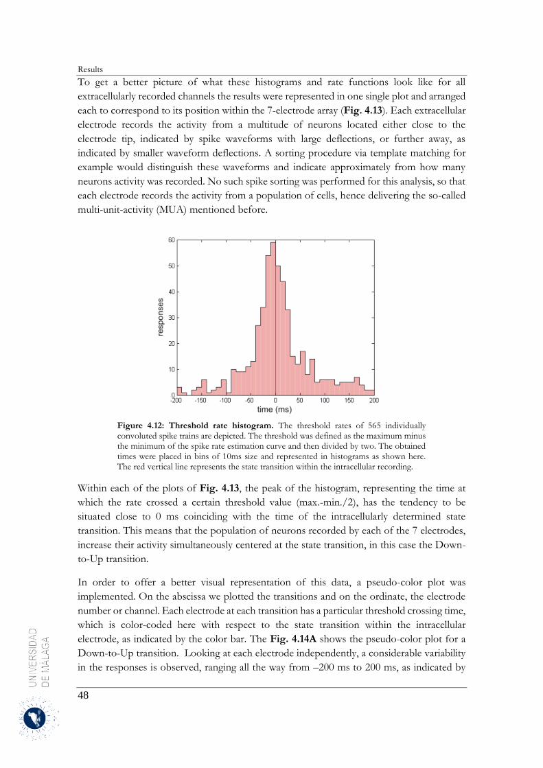
Results
48
To get a better picture of what these histograms and rate functions look like for all
extracellularly recorded channels the results were represented in one single plot and arranged
each to correspond to its position within the 7-electrode array (Fig. 4.13). Each extracellular
electrode records the activity from a multitude of neurons located either close to the
electrode tip, indicated by spike waveforms with large deflections, or further away, as
indicated by smaller waveform deflections. A sorting procedure via template matching for
example would distinguish these waveforms and indicate approximately from how many
neurons activity was recorded. No such spike sorting was performed for this analysis, so that
each electrode records the activity from a population of cells, hence delivering the so-called
multi-unit-activity (MUA) mentioned before.
Figure 4.12: Threshold rate histogram. The threshold rates of 565 individually convoluted spike trains are depicted. The threshold was defined as the maximum minus the minimum of the spike rate estimation curve and then divided by two. The obtained times were placed in bins of 10ms size and represented in histograms as shown here. The red vertical line represents the state transition within the intracellular recording.
Within each of the plots of Fig. 4.13, the peak of the histogram, representing the time at
which the rate crossed a certain threshold value (max.-min./2), has the tendency to be
situated close to 0 ms coinciding with the time of the intracellularly determined state
transition. This means that the population of neurons recorded by each of the 7 electrodes,
increase their activity simultaneously centered at the state transition, in this case the Down-
to-Up transition.
In order to offer a better visual representation of this data, a pseudo-color plot was
implemented. On the abscissa we plotted the transitions and on the ordinate, the electrode
number or channel. Each electrode at each transition has a particular threshold crossing time,
which is color-coded here with respect to the state transition within the intracellular
electrode, as indicated by the color bar. The Fig. 4.14A shows the pseudo-color plot for a
Down-to-Up transition. Looking at each electrode independently, a considerable variability
in the responses is observed, ranging all the way from –200 ms to 200 ms, as indicated by

Results
49
the different colors. Any transition left blank, or white, corresponded to trials removed via
the Mann-Whitney U test. Comparing the threshold crossing times between electrodes, in
this representation of the data, the variability is such that there is no unique pattern in the
activity spreading across the electrodes.
Figure 4.13: Spike train alignments to the Down-to-Up transitions. The single trial rate estimations for 565 Down-to-Up transitions are depicted in light gray curves. The threshold crossing of each of these rate estimations are represented by the histograms (bin size 10ms). The average of the 565 individual rate estimation profiles (mean) is depicted by the blue curve. These seven plots (Ch1-7 according to seven recording channels) correspond to the recordings of each of the seven extracellular microelectrodes as located in the 7-electrode array. The arrangement thus is equivalent to the position of the electrodes in this particular array. In all recording channels, the histogram peak is located around 0 ms, indicating that all electrodes tend to cross the threshold simultaneous to the state transition occurring in the intracellular recoding (red vertical line). Hence, the recorded MUA from a total of seven electrodes positioned within a cortical area of size 400x400 µm increases at the same time coinciding with the state transitions detected in the intracellular recorded neuron.
For a further analysis of this data and determine if there is a pattern in the spreading activity,
the average (mean) threshold crossing time and its corresponding standard deviation was
calculated (Fig. 4.14B) observing that electrode 3, in this example, has the smallest average
value, meaning that, in comparison to the other electrodes, its MUA increases the earliest.
Based on the hypothesis that the discharge caused in this electrode is due to a propagating
wave front, an approximation regarding its direction can be made: The propagating wave
front has its origin at electrode 3, travels onward to electrodes 4 and 7, then passing electrode
2 and 1.

Results
50
Figure 4.14: Down-to-Up state transition times of MUA. A. Pseudo-colored plot depicts the threshold crossing times of all seven electrodes in the array, where each color represents a specific time (ranging from -200 to 200ms) being 0 ms the state transition as determined by the intracellularly recorded neuron. All values are thus compared to this state transition. In this representation of data, within a single electrode, the threshold crossing times show a high variability not allowing to elucidate any pattern. Nevertheless, additional analysis depicted in B, where the mean threshold crossing times for each electrode and the standard deviation (StD) were determined, show that electrode 3 tends to cross threshold first followed by electrodes 4, and 7, passing to electrode 2 and then electrodes 1 and 6, being electrode 5 the last to cross state transition threshold.
Finally, the activity reaches electrodes 6 and 5. This rather unusual direction of propagation
can be pointed out by averaging not only the individual threshold crossing time values but
also their corresponding color (Fig. 4.15).
Figure 4.15: Spreading activity in the Down-to-Up transition. Wave propagation analysis for the Down-to-Up transitions. Each square represents the average color of the threshold crossing times and its location, the position of the electrodes in the array. Upon visual inspection, the direction of activity propagation starts in the lower electrode row and moves diagonally, ending in the upper right corner of the array as indicated by the arrow.
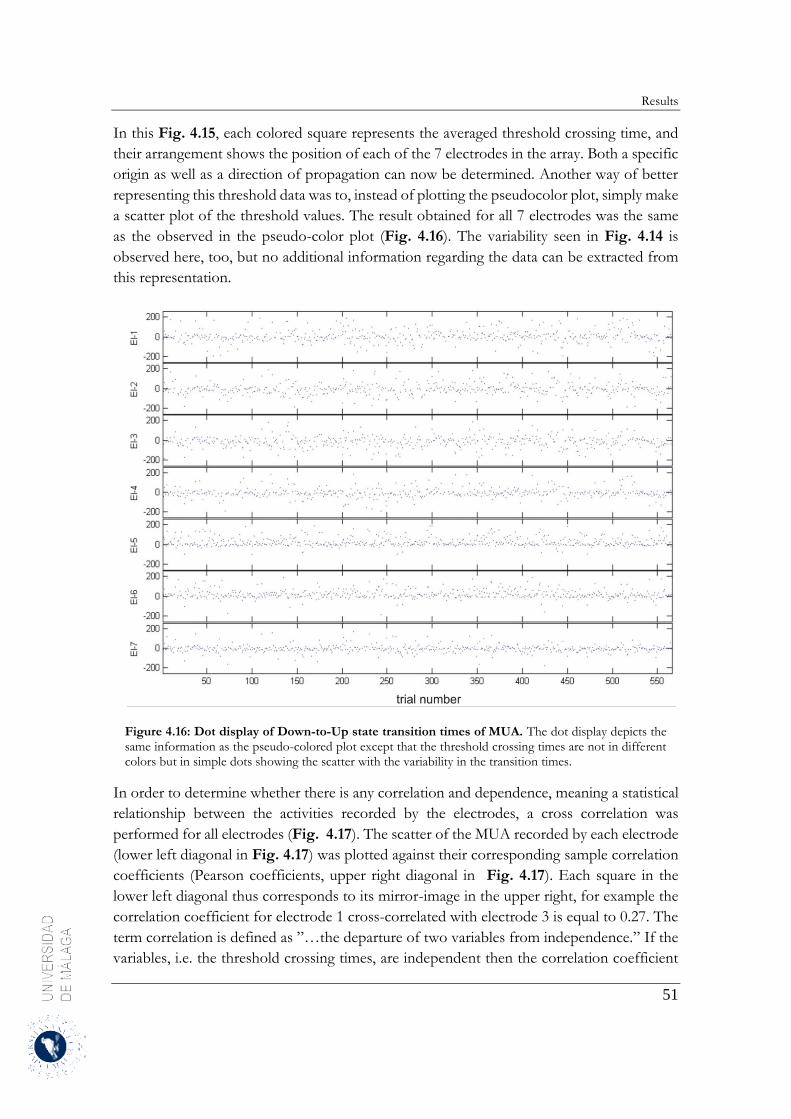
Results
51
In this Fig. 4.15, each colored square represents the averaged threshold crossing time, and
their arrangement shows the position of each of the 7 electrodes in the array. Both a specific
origin as well as a direction of propagation can now be determined. Another way of better
representing this threshold data was to, instead of plotting the pseudocolor plot, simply make
a scatter plot of the threshold values. The result obtained for all 7 electrodes was the same
as the observed in the pseudo-color plot (Fig. 4.16). The variability seen in Fig. 4.14 is
observed here, too, but no additional information regarding the data can be extracted from
this representation.
Figure 4.16: Dot display of Down-to-Up state transition times of MUA. The dot display depicts the same information as the pseudo-colored plot except that the threshold crossing times are not in different colors but in simple dots showing the scatter with the variability in the transition times.
In order to determine whether there is any correlation and dependence, meaning a statistical
relationship between the activities recorded by the electrodes, a cross correlation was
performed for all electrodes (Fig. 4.17). The scatter of the MUA recorded by each electrode
(lower left diagonal in Fig. 4.17) was plotted against their corresponding sample correlation
coefficients (Pearson coefficients, upper right diagonal in Fig. 4.17). Each square in the
lower left diagonal thus corresponds to its mirror-image in the upper right, for example the
correlation coefficient for electrode 1 cross-correlated with electrode 3 is equal to 0.27. The
term correlation is defined as ”…the departure of two variables from independence.” If the
variables, i.e. the threshold crossing times, are independent then the correlation coefficient
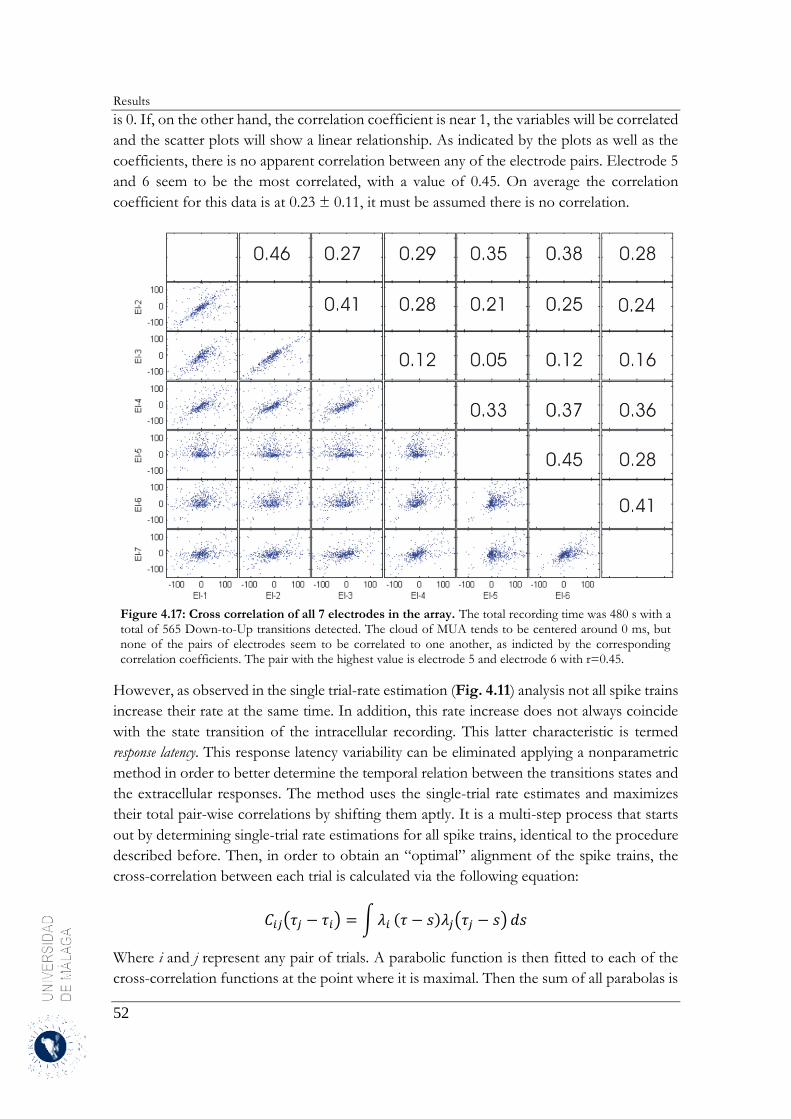
Results
52
is 0. If, on the other hand, the correlation coefficient is near 1, the variables will be correlated
and the scatter plots will show a linear relationship. As indicated by the plots as well as the
coefficients, there is no apparent correlation between any of the electrode pairs. Electrode 5
and 6 seem to be the most correlated, with a value of 0.45. On average the correlation
coefficient for this data is at 0.23 ± 0.11, it must be assumed there is no correlation.
Figure 4.17: Cross correlation of all 7 electrodes in the array. The total recording time was 480 s with a total of 565 Down-to-Up transitions detected. The cloud of MUA tends to be centered around 0 ms, but none of the pairs of electrodes seem to be correlated to one another, as indicted by the corresponding correlation coefficients. The pair with the highest value is electrode 5 and electrode 6 with r=0.45.
However, as observed in the single trial-rate estimation (Fig. 4.11) analysis not all spike trains
increase their rate at the same time. In addition, this rate increase does not always coincide
with the state transition of the intracellular recording. This latter characteristic is termed
response latency. This response latency variability can be eliminated applying a nonparametric
method in order to better determine the temporal relation between the transitions states and
the extracellular responses. The method uses the single-trial rate estimates and maximizes
their total pair-wise correlations by shifting them aptly. It is a multi-step process that starts
out by determining single-trial rate estimations for all spike trains, identical to the procedure
described before. Then, in order to obtain an “optimal” alignment of the spike trains, the
cross-correlation between each trial is calculated via the following equation:
𝐶𝑖𝑗(𝜏𝑗 − 𝜏𝑖) = ∫𝜆𝑖 (𝜏 − 𝑠)𝜆𝑗(𝜏𝑗 − 𝑠) 𝑑𝑠
Where i and j represent any pair of trials. A parabolic function is then fitted to each of the
cross-correlation functions at the point where it is maximal. Then the sum of all parabolas is
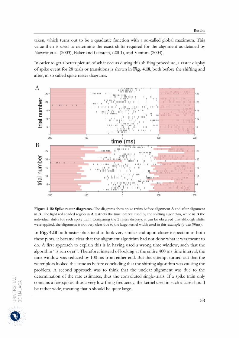
Results
53
taken, which turns out to be a quadratic function with a so-called global maximum. This
value then is used to determine the exact shifts required for the alignment as detailed by
Nawrot et al. (2003), Baker and Gerstein, (2001), and Ventura (2004).
In order to get a better picture of what occurs during this shifting procedure, a raster display
of spike event for 28 trials or transitions is shown in Fig. 4.18, both before the shifting and
after, in so called spike raster diagrams.
Figure 4.18: Spike raster diagrams. The diagrams show spike trains before alignment A and after alignment
in B. The light red shaded region in A restricts the time interval used by the shifting algorithm, while in B the
individual shifts for each spike train. Comparing the 2 raster displays, it can be observed that although shifts
were applied, the alignment is not very clear due to the large kernel width used in this example (σ was 90ms).
In Fig. 4.18 both raster plots tend to look very similar and upon closer inspection of both
these plots, it became clear that the alignment algorithm had not done what it was meant to
do. A first approach to explain this is in having used a wrong time window, such that the
algorithm “is run over”. Therefore, instead of looking at the entire 400 ms time interval, the
time window was reduced by 100 ms from either end. But this attempt turned out that the
raster plots looked the same as before concluding that the shifting algorithm was causing the
problem. A second approach was to think that the unclear alignment was due to the
determination of the rate estimates, thus the convoluted single-trials. If a spike train only
contains a few spikes, thus a very low firing frequency, the kernel used in such a case should
be rather wide, meaning that σ should be quite large.
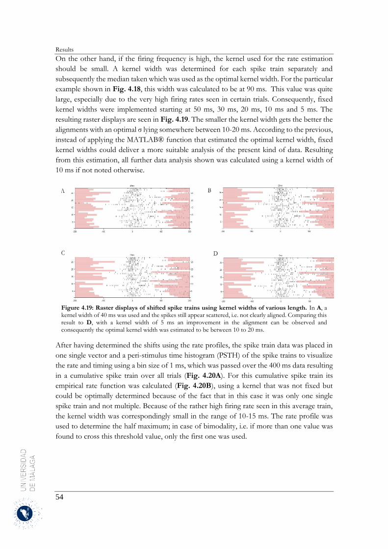
Results
54
On the other hand, if the firing frequency is high, the kernel used for the rate estimation
should be small. A kernel width was determined for each spike train separately and
subsequently the median taken which was used as the optimal kernel width. For the particular
example shown in Fig. 4.18, this width was calculated to be at 90 ms. This value was quite
large, especially due to the very high firing rates seen in certain trials. Consequently, fixed
kernel widths were implemented starting at 50 ms, 30 ms, 20 ms, 10 ms and 5 ms. The
resulting raster displays are seen in Fig. 4.19. The smaller the kernel width gets the better the
alignments with an optimal σ lying somewhere between 10-20 ms. According to the previous,
instead of applying the MATLAB® function that estimated the optimal kernel width, fixed
kernel widths could deliver a more suitable analysis of the present kind of data. Resulting
from this estimation, all further data analysis shown was calculated using a kernel width of
10 ms if not noted otherwise.
Figure 4.19: Raster displays of shifted spike trains using kernel widths of various length. In A, a kernel width of 40 ms was used and the spikes still appear scattered, i.e. not clearly aligned. Comparing this result to D, with a kernel width of 5 ms an improvement in the alignment can be observed and consequently the optimal kernel width was estimated to be between 10 to 20 ms.
After having determined the shifts using the rate profiles, the spike train data was placed in
one single vector and a peri-stimulus time histogram (PSTH) of the spike trains to visualize
the rate and timing using a bin size of 1 ms, which was passed over the 400 ms data resulting
in a cumulative spike train over all trials (Fig. 4.20A). For this cumulative spike train its
empirical rate function was calculated (Fig. 4.20B), using a kernel that was not fixed but
could be optimally determined because of the fact that in this case it was only one single
spike train and not multiple. Because of the rather high firing rate seen in this average train,
the kernel width was correspondingly small in the range of 10-15 ms. The rate profile was
used to determine the half maximum; in case of bimodality, i.e. if more than one value was
found to cross this threshold value, only the first one was used.
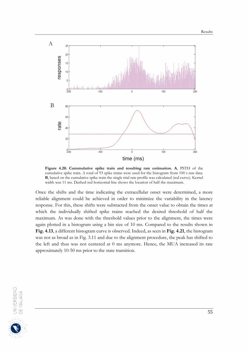
Results
55
Figure 4.20: Cummulative spike train and resulting rate estimation. A, PSTH of the cumulative spike train. A total of 93 spike trains were used for the histogram from 100 s raw data. B, based on the cumulative spike train the single trial rate profile was calculated (red curve). Kernel width was 11 ms. Dashed red horizontal line shows the location of half the maximum.
Once the shifts and the time indicating the extracellular onset were determined, a more
reliable alignment could be achieved in order to minimize the variability in the latency
response. For this, these shifts were subtracted from the onset value to obtain the times at
which the individually shifted spike trains reached the desired threshold of half the
maximum. As was done with the threshold values prior to the alignment, the times were
again plotted in a histogram using a bin size of 10 ms. Compared to the results shown in
Fig. 4.13, a different histogram curve is observed. Indeed, as seen in Fig. 4.21, the histogram
was not as broad as in Fig. 3.11 and due to the alignment procedure, the peak has shifted to
the left and thus was not centered at 0 ms anymore. Hence, the MUA increased its rate
approximately 10-50 ms prior to the state transition.
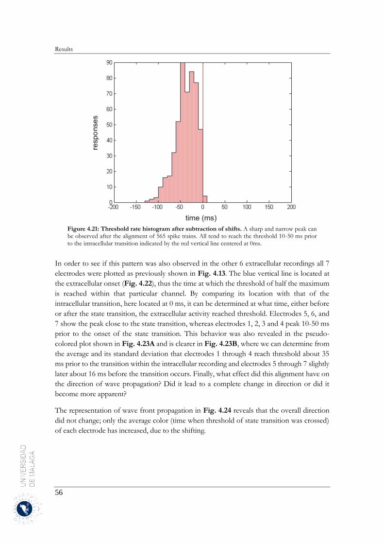
Results
56
Figure 4.21: Threshold rate histogram after subtraction of shifts. A sharp and narrow peak can be observed after the alignment of 565 spike trains. All tend to reach the threshold 10-50 ms prior to the intracellular transition indicated by the red vertical line centered at 0ms.
In order to see if this pattern was also observed in the other 6 extracellular recordings all 7
electrodes were plotted as previously shown in Fig. 4.13. The blue vertical line is located at
the extracellular onset (Fig. 4.22), thus the time at which the threshold of half the maximum
is reached within that particular channel. By comparing its location with that of the
intracellular transition, here located at 0 ms, it can be determined at what time, either before
or after the state transition, the extracellular activity reached threshold. Electrodes 5, 6, and
7 show the peak close to the state transition, whereas electrodes 1, 2, 3 and 4 peak 10-50 ms
prior to the onset of the state transition. This behavior was also revealed in the pseudo-
colored plot shown in Fig. 4.23A and is clearer in Fig. 4.23B, where we can determine from
the average and its standard deviation that electrodes 1 through 4 reach threshold about 35
ms prior to the transition within the intracellular recording and electrodes 5 through 7 slightly
later about 16 ms before the transition occurs. Finally, what effect did this alignment have on
the direction of wave propagation? Did it lead to a complete change in direction or did it
become more apparent?
The representation of wave front propagation in Fig. 4.24 reveals that the overall direction
did not change; only the average color (time when threshold of state transition was crossed)
of each electrode has increased, due to the shifting.
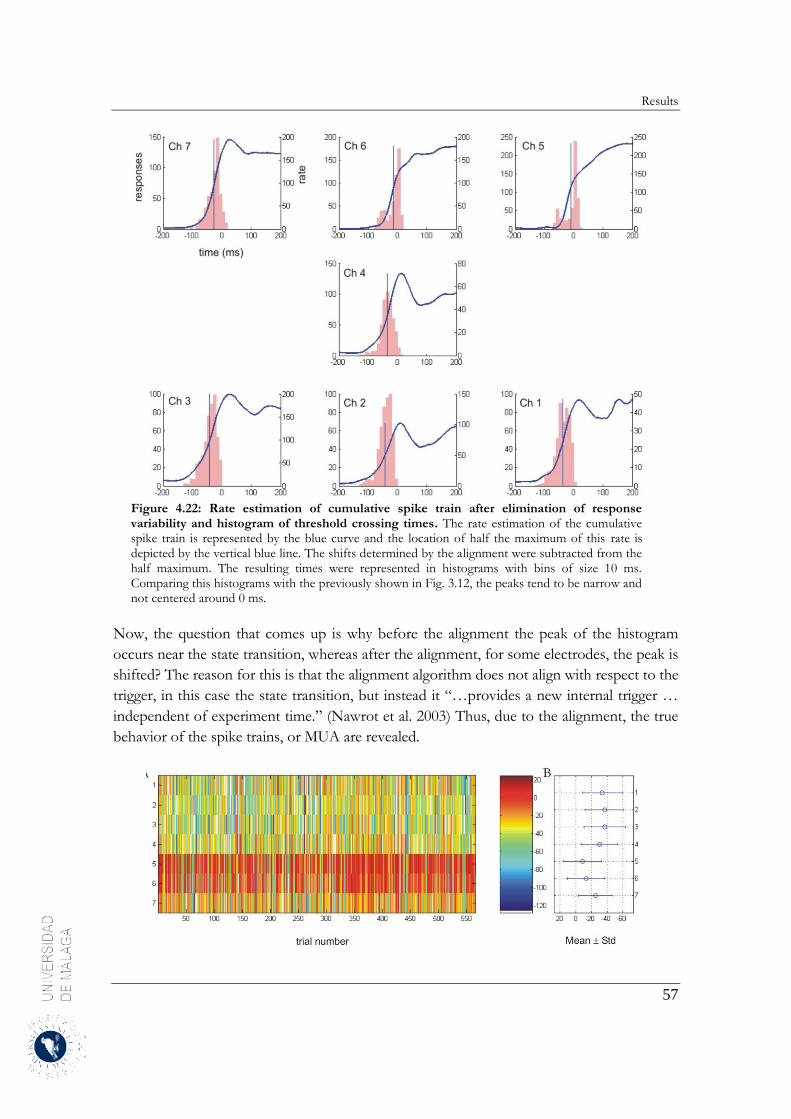
Results
57
Figure 4.22: Rate estimation of cumulative spike train after elimination of response variability and histogram of threshold crossing times. The rate estimation of the cumulative spike train is represented by the blue curve and the location of half the maximum of this rate is depicted by the vertical blue line. The shifts determined by the alignment were subtracted from the half maximum. The resulting times were represented in histograms with bins of size 10 ms. Comparing this histograms with the previously shown in Fig. 3.12, the peaks tend to be narrow and not centered around 0 ms.
Now, the question that comes up is why before the alignment the peak of the histogram
occurs near the state transition, whereas after the alignment, for some electrodes, the peak is
shifted? The reason for this is that the alignment algorithm does not align with respect to the
trigger, in this case the state transition, but instead it “…provides a new internal trigger …
independent of experiment time.” (Nawrot et al. 2003) Thus, due to the alignment, the true
behavior of the spike trains, or MUA are revealed.
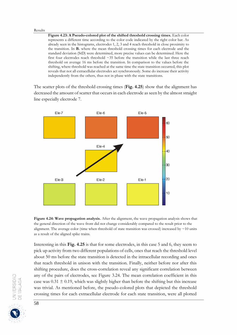
Results
58
Figure 4.23: A Pseudo-colored plot of the shifted threshold crossing times. Each color represents a different time according to the color code indicated by the right color bar. As already seen in the histograms, electrodes 1, 2, 3 and 4 reach threshold in close proximity to the transition. In B. where the mean threshold crossing times for each electrode and the standard deviation (StD) were determined, more precise values can be determined. Here the first four electrodes reach threshold ~35 before the transition while the last three reach threshold on average 16 ms before the transition. In comparison to the values before the shifting, where threshold was reached at the same time the state transition occurred, this plot reveals that not all extracellular electrodes act synchronously. Some do increase their activity independently from the others, thus not in phase with the state transitions.
The scatter plots of the threshold crossing times (Fig. 4.25) show that the alignment has
decreased the amount of scatter that occurs in each electrode as seen by the almost straight
line especially electrode 7.
Figure 4.24: Wave propagation analysis. After the alignment, the wave propagation analysis shows that
the general direction of the wave front did not change considerably compared to the result prior to the
alignment. The average color (time when threshold of state transition was crossed) increased by ~10 units
as a result of the aligned spike trains.
Interesting in this Fig. 4.25 is that for some electrodes, in this case 5 and 6, they seem to
pick up activity from two different populations of cells, ones that reach the threshold level
about 50 ms before the state transition is detected in the intracellular recording and ones
that reach threshold in unison with the transition. Finally, neither before nor after this
shifting procedure, does the cross-correlation reveal any significant correlation between
any of the pairs of electrodes, see Figure 3.24. The mean correlation coefficient in this
case was 0.31 ± 0.19, which was slightly higher than before the shifting but this increase
was trivial. As mentioned before, the pseudo-colored plots that depicted the threshold
crossing times for each extracellular electrode for each state transition, were all plotted

Results
59
relative to the intracellular recording, meaning relative to 0 ms.
Figure 4.25: Scatter plot (left) showing the threshold crossing times after the alignment procedure and crosscorrelation (right). In the scatter plot after the alignment procedure the amount of scatter decreased compared to Fig. 4.15. Electrodes 5 and 6 seem to record activity from two different populations of cells, ones that reach threshold at ~50 ms before the state transition, the other reach threshold simultaneous to the state transition. In the crosscorrelogram the lower left depicts the scatter plots of each electrode pair and the upper right their corresponding correlation coefficient. Electrode pair with the highest correlation: electrode 2 and 3, r=0.74. Mean correlation coefficient is 0.31±0.19, slightly higher than before shifting, i.e. no significant correlation between any of the pairs of electrodes in this seven electrode array.
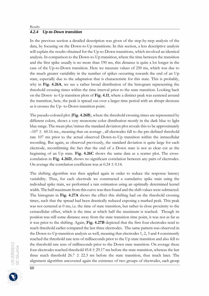
Results
60
4.2.4 Up-to-Down transition
In the previous section a detailed description was given of the step-by-step analysis of the
data, by focusing on the Down-to-Up transitions. In this section, a less descriptive analysis
will explain the results obtained for the Up-to-Down transitions, which involved an identical
analysis. In comparison to the Down-to-Up transition, where the time between the transition
and the first spike usually is no more than 190 ms, this distance is quite a lot longer in the
case of the Up-to-Down transition. Here we measure values of 250 ms, which was due to
the much greater variability in the number of spikes occurring towards the end of an Up
state, especially due to the adaptation that is characteristic for this state. This is probably,
why in Fig. 4.26A, we see a rather broad distribution of the histogram representing the
threshold crossing times within the time interval prior to the state transition. Looking back
on the Down- to-Up transition plots of Fig. 4.11, where a distinct peak was centered around
the transition, here, the peak is spread out over a larger time period with an abrupt decrease
as it crosses the Up- to-Down transition point.
The pseudo-colored plot (Fig. 4.26B), where the threshold crossing times are represented by
different colors, shows a very monotone color distribution mostly in the dark blue to light
blue range. The mean plus/minus the standard deviation plot reveals this to be approximately
–107 ± 60.16 ms., meaning that on average , all electrodes fall to the pre-defined threshold
rate 107 ms prior to the actual observed Down-to-Up transition within the intracellular
recording. But again, as observed previously, the standard deviation is quite large for each
electrode, reconfirming the fact that the end of a Down state is not as clear cut as the
beginning of an Up state. Fig. 4.26C shows the same data as a scatter plot. The cross-
correlation in Fig. 4.26D, shows no significant correlation between any pairs of electrodes.
On average the correlation coefficient was at 0.24 ± 0.14.
The shifting algorithm was then applied again in order to reduce the response latency
variability. Thus, for each electrode we constructed a cumulative spike train using the
individual spike train, we performed a rate estimation using an optimally determined kernel
width. The half maximum from this curve was then found and the shift values were subtracted.
The histogram in Fig. 4.27A shows the effect this shifting had on the threshold crossing
times, such that the spread had been drastically reduced exposing a marked peak. This peak
was not centered at 0 ms, i.e. the time of state transition, but rather in close proximity to the
extracellular offset, which is the time at which half the maximum is reached. Though its
position was still some distance away from the state transition time point, it was not as far as
it was prior to the shifting. Again, Fig. 4.27B depicted that the first four electrodes tend to
reach threshold earlier compared the last three electrodes. The same pattern was observed in
the Down-to-Up transition analysis as well, meaning that electrodes 1, 2, 3 and 4 consistently
reached the threshold rate tens of milliseconds prior to the Up state transition and also fell to
the threshold rate tens of milliseconds prior to the Down state transition. On average these
four electrodes reached threshold 45.8 ± 29.17 ms before the state transition, whereas the last
three reach threshold 26.7 ± 22.3 ms before the state transition, thus much later. The
alignment algorithm uncovered again the existence of two groups of electrodes, each group
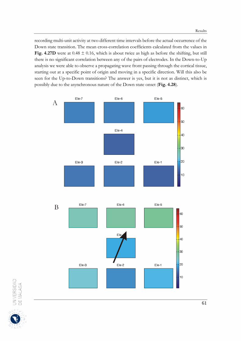
Results
61
recording multi-unit activity at two different time intervals before the actual occurrence of the
Down state transition. The mean cross-correlation coefficients calculated from the values in
Fig. 4.27D were at 0.48 ± 0.16, which is about twice as high as before the shifting, but still
there is no significant correlation between any of the pairs of electrodes. In the Down-to-Up
analysis we were able to observe a propagating wave front passing through the cortical tissue,
starting out at a specific point of origin and moving in a specific direction. Will this also be
seen for the Up-to-Down transitions? The answer is yes, but it is not as distinct, which is
possibly due to the asynchronous nature of the Down state onset (Fig. 4.28).

Results
62
Figure 4.28: Wave propagation analysis before – A and after - B alignment for Up-to-Down
transitions. In both cases the direction of the wave front is difficult to decipher, possible caused by the
asynchronous nature of the onset of the Down state. In B according to the color code the most likely
direction is the one indicated by the arrow.

Conclusions
63
Figure 4.26: Up-to-Down transition analysis. A As previously explained, each plot depicts the rate estimates for each state transition, here Up to Down drawn as gray curves. The histograms
shows the threshold crossing times with respect to the intracellularly detected transition (red vertical line). The blue curve line is the mean of the convoluted single trial rate estimates.
Comparing this to the Down to Up analysis before, the histogram in this case does not have a sharp peak, but a rather broad distribution spread all along the Up state time interval (-200-0 ms).
The arrangement of the seven plots illustrates the position of the 7 electrodes in the extracellular array. B The pseudo-colored plot “color-codes” the threshold crossing times depicting the
variability in the spike firing at the end of an Up state, the electrodes tend to decrease their firing rate 90-125 ms prior to the actual state transition
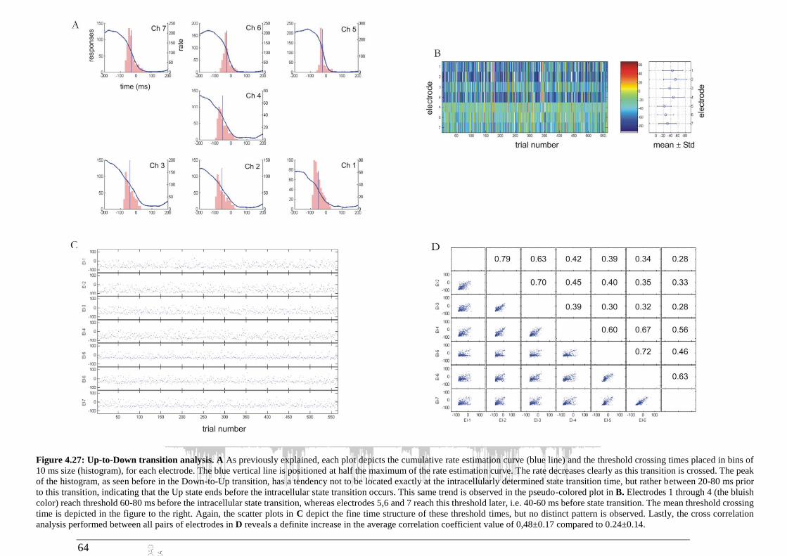
64
Figure 4.27: Up-to-Down transition analysis. A As previously explained, each plot depicts the cumulative rate estimation curve (blue line) and the threshold crossing times placed in bins of
10 ms size (histogram), for each electrode. The blue vertical line is positioned at half the maximum of the rate estimation curve. The rate decreases clearly as this transition is crossed. The peak
of the histogram, as seen before in the Down-to-Up transition, has a tendency not to be located exactly at the intracellularly determined state transition time, but rather between 20-80 ms prior
to this transition, indicating that the Up state ends before the intracellular state transition occurs. This same trend is observed in the pseudo-colored plot in B. Electrodes 1 through 4 (the bluish
color) reach threshold 60-80 ms before the intracellular state transition, whereas electrodes 5,6 and 7 reach this threshold later, i.e. 40-60 ms before state transition. The mean threshold crossing
time is depicted in the figure to the right. Again, the scatter plots in C depict the fine time structure of these threshold times, but no distinct pattern is observed. Lastly, the cross correlation
analysis performed between all pairs of electrodes in D reveals a definite increase in the average correlation coefficient value of 0,48±0.17 compared to 0.24±0.14.
Discussion
65
5 Discussion
Slow waves are generated by the cortical network and they recruit the thalamo-cortical loop,
engaging many brain areas during both slow wave sleep and anesthesia (Steriade et al., 1993d;
McCormick et al., 2003; Sakata and Harris, 2009; Ruiz-Mejias et al., 2011; Stroh et al., 2013).
Slow waves can be considered the default activity of the cortical network (Sanchez-Vives &
Mattia, 2014) and by exploring in detail the generation and propagation properties of the
slow oscillations, we can extract information about how the cortical network functions under
control conditions or in models of disease. The process of extracting information from the
physiology requires sophisticated analytical tools. This Thesis consisted in a large part in the
development of such analytical tools: one to detect slow oscillations in intracellular
recordings and the other one to analyze an array of multiple recordings and measure
correlation and propagation properties of the activity. In order to test the methods I made
use of data collected by collaborators and data obtained from my own in vivo experiments.
5.1 Robust off- and online identification of intracellularly recorded
Up and Down cortical states
Identifying the transitions between Up and Down cortical states is sometimes difficult and
has to rely on the subjective opinion of the researcher. For example, it is not clear when a
short depolarization should be wide enough to be considered an Up state or when the
absence of spikes is a necessary condition to determine the presence of a Down state.
Understanding the cellular and network mechanisms that generate the two-state behavior
generated by the cortical network demands a robust and reliable method for Up and Down
states identification. Here we have demonstrated that the traditional histogram-based
approach originally described by Metherate and Ashe (1993) and extensively used afterwards
(e.g. Sanchez-Vives et al., 2000; Petersen et al., 2003; Anderson et al., 2000; Benucci et al,
2004; Crochet et al., 2004; Fuentealba & Steriade, 2005; Kasanetz et al., 2002; Lewis &
O’Donnell, 2000; Mahon et al., 2003; Peters et al., 2004; Timofeev et al., 2001; Tseng et al.,
2001) while being an efficient graphical tool for manual threshold determination under ideal
conditions, lacks the adaptive computational properties to deal with fuzzy transitions,
occurring during recordings that are not stable, or drifting, that develops quite often over
long recordings.
Trend-following techniques of financial trading applications combined with problem-
specific knowledge yields a method that robustly separates Up and Down states, in both ideal
and fuzzy situations. This thesis formalizes such a method and analyses its performance in
different situations characteristic of ill-defined biphasic behavior: (1) irregular shape of Up
and Down states –variations in amplitude, frequency– (Fig. 4.3) (2) imprecise Down state
initiation, (3) signal drifting (caused by changes in the liquid junction potential at the
Discussion
66
electrode tip), or (4) artifacts due to movements during in vivo recordings, such as respiratory
movements or heartbeat (Fig. 2).
The experiments carried out for Up and Down state identification show that histogram-
based methods will perform well in ideal situations (as widely reported in the literature), but
will fail if the signal differs from this harmonic, well-defined and non-trended behavior. On
the other hand, MAUDS efficiently separates Up and Down states in ideal (closely fitting the
best histogram-based characterization) as well as in irregular oscillation. The cases studied
in this work are common in most intracellular recordings, and can be analyzed with an
adaptive method of the sort of MAUDS.
Well-defined Up and Down states have been widely studied in the past, but how this bi-
stable behavior departs from ideal conditions has not been reported in the literature, perhaps
because of the lack of objective methods to characterize irregular situations. Such a method
will allow formal quantification of these excursions, and must be based on an extended
definition of the Up and Down states that meets conflicting experimenters’ criteria. An
algorithmic approach similar to the one presented here would definitely be a good starting
point in this direction.
In order to integrate the online and offline versions, the model has been defined and tested
with EMAs that compute only previous values. This is at the cost of a delay in the turning
points obtained, which affects the overall performance. An offline version based on EMAs
that average past and future intervals of time for each value would improve the results shown
here. In spite of this delay, the predictive character of the online version has been used
experimentally to trigger stimuli and to manipulate cell membrane voltage at specific times
along the oscillation. This is of great interest for experimentalists studying the responses to
sensory stimulation during Up or Down states. Exponential weighting has proved to
perform well, since it reacts faster, minimizing the lag between the predictive moving average
and the actual data. The method is also expected to perform well in this type of interactive
experiments, since the presence of sensory stimuli, current injection, or other manipulations
interspersed with the oscillation will not interfere with the turning points. Only the presence
of short Down states might be problematic, since the artifacts might cut them. The general
approach exposed here would be easily fitted to the conditions of particular experimental
settings.
The method formalized in this paper has been coded as a Spike2 script, an assembly program,
and also embedded in a MATLAB® toolbox. All these programs are available online as an
open-source code. The MATLAB® implementation exploits fast matrix operations and the
powerful graphical capabilities of this programming language, and can analyze
electrophysiological raw data formatted as ASCII or MATLAB® binary files. The code has
been optimized and computes more than a million membrane potential samples per second
on a PIV 2.8GHz with 0.5GB memory (this computer processes a file containing 10 minutes
of intracellular membrane potential sampled at 25 kHz in some 13 seconds). On the other
hand, the Spike 2 implementations are designed for online data processing, allowing real-
Discussion
67
time characterization and visualization (script version), and triggering of stimuli (sequencer
version).
Further work has to be done in order to improve two different aspects of MAUDS: (1) the
adaptive capabilities of the proposed method, by automatically setting the window size of
the fast EMA, that can be done based on local membrane potential variability, or exploring
ranges of values where the identification remains stable; and (2) a complete validation of
MAUDS over an extensive set of intracellular data recorded in different cortical areas. While
a good general performance is expected, even with minor changes in the parameter set, the
forum set up in the MAUDS website is expected to feedback about this question, as more
experimenters report on the application of MAUDS to recorded datasets.
Discussion
68
5.2 Spatio-temporal structure of spontaneous slow-wave oscillations
in the neocortex
As said above, the slow oscillation recorded during slow wave sleep or during certain
anesthetics represents a spontaneous event during which cortical neurons are alternately
silent and active for a fraction of a second. These spontaneous state transitions of neocortical
activity are characterized by fast changes between epochs of intense network activity (Up
states), and quiescent periods, where spiking activity is virtually absent (Down states). In
single cells, Up states are characterized by massive synaptic input, leading to a strongly
fluctuating, depolarizing membrane potential, while in Down states, the membrane potential
shows only few fluctuations at a hyperpolarized level.
The final objective of my research was to unveil the spatio-temporal structure of
spontaneous slow-wave oscillations in the rat somatosensory cortex. With that purpose, we
firstly tried to determine whether the characteristic slow oscillations observed during slow-
wave sleep (SWS) lead to the induction of propagating wave fronts that start out at a specific
origin and travel in a given direction through the cortical tissue. The velocity of this traveling
wave depends on the complexity of the network circuitry. For this study, we implemented a
spatially defined array of seven extracellular electrodes in combination with one intracellular
electrode and recorded from the somatosensory cortex of rats anesthetized with a
combination of urethane and ketamine/xylazine. This kind of anesthesia has been
established as a model for slow-wave sleep (Fontanini et al. 2003; Sharma et al. 2010) and
leads to stable and regular low-frequency oscillations in the neocortex. Although the state
transitions also occur under urethane anesthesia alone, the use of ketamine enhances and
stabilizes the appearance of Up and Down states.
The extracellular recordings using arrays consisting of 7 electrodes, made it possible to
measure multi-unit activity ideally within a cortical layer. It was found that these propagating
waves of activity show considerable variability with regard to their spatiotemporal pattern.
However, a unique point of origin and direction could be identified for at least each wave.
Whether this is true for each recording session cannot be asserted as this might at least
depend on the length of each of these recording sessions.
Regarding the laminar distribution, both in vitro and in vivo recordings position the origin of
oscillations in deep (layers 5 and 6) layers. Sanchez-Vives & McCormick (2000), positioning
their electrodes perpendicular to the pia, observed that activity tended to start in layer 5,
followed within a short delay (~32 ms) by activity in layer 6, and finally reaching layer 2/3.
In vivo recordings agree in the observation of an initiation of slow oscillations in the
infragranular or deep cortical layers (Sakata & Harris, 2009; Chauvette et al., 2010). But, how
do oscillations travel across the cortex?
Massimini et al. (2004) demonstrated by combining sleep-EEG recordings and MRI that the

Discussion
69
vast majority of the slow oscillation cycles could be characterized by an origin and a
continuous pathway of propagation, as it is the case for a travelling wave all over the cortex.
According to this, each slow oscillation has a definite site of origin and direction of
propagation, which vary from one cycle to the next. Furthermore, it was shown that the slow
oscillation could originate from almost any area of the scalp and propagates in every
direction, although certain origins and directions of propagation occurred more frequently
than others. More recent measurements by means of calcium imaging in rodents also find a
predominant front to back propagation (Stroh et al 2013). Still, a detailed description bridging
micro and mesoscales was missing.
The results of this Thesis showed that in most recordings there was considerable variability
with respect to the precise spatio-temporal structure of activity waves (Fig. 5.1A). These
plots illustrate the variability of the wave front, both in origin and direction for different
animals.
However, in many cases a preferred direction of activity spread could be identified during
limited recording periods. Within a single recording session though, lasting up to 12 minutes,
the wave front tended to remain quite constant, which suggests that the waves of activity
seen during SWS travel in a stereotypic manner through the cortical layer. This also indicates
that under ketamine/xylazine anesthesia, activity waves may travel in a stereotypic manner
over the neocortical tissue. Such stereotypic patterns of activity might lead to selective
strengthening of active synapses, linking slow-wave activity to learning-related phenomena
like memory consolidation during slow-wave sleep (Marshall et al., 2006)
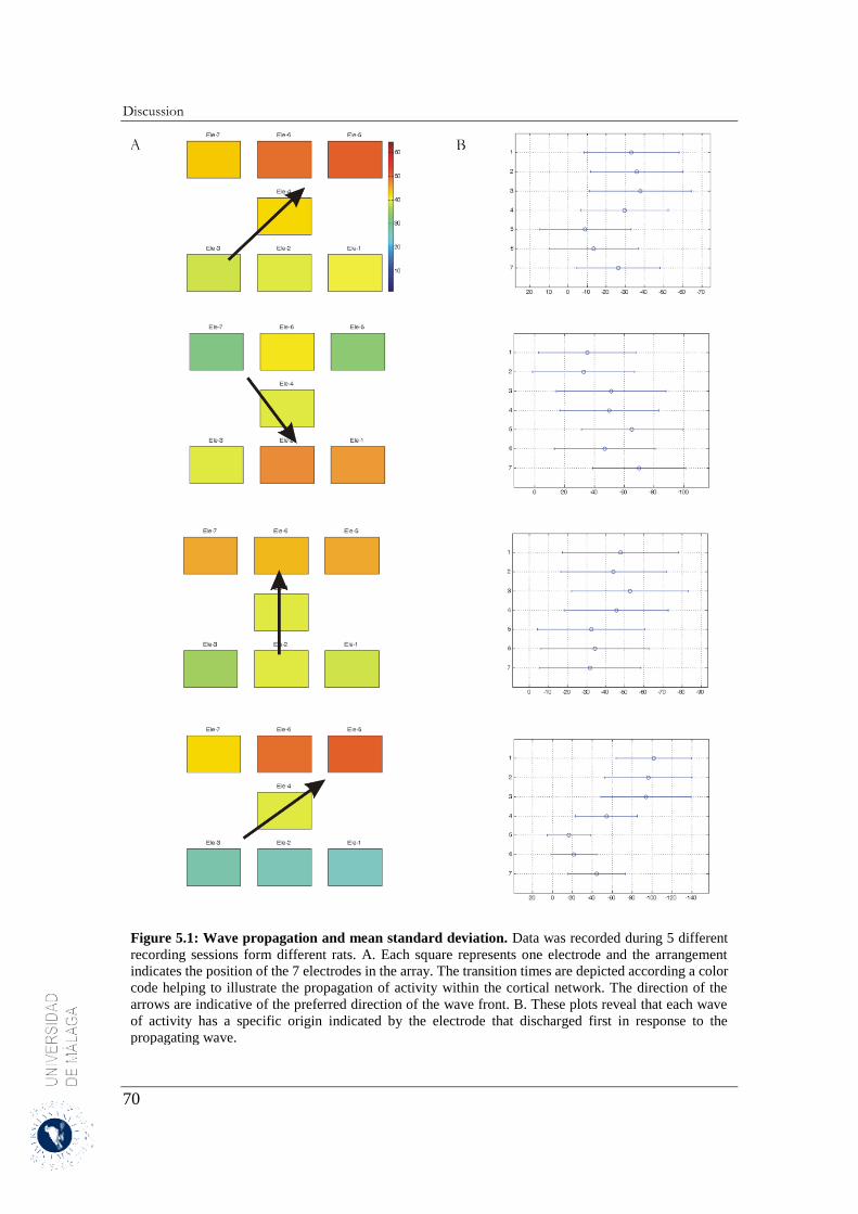
Discussion
70
Figure 5.1: Wave propagation and mean standard deviation. Data was recorded during 5 different
recording sessions form different rats. A. Each square represents one electrode and the arrangement
indicates the position of the 7 electrodes in the array. The transition times are depicted according a color
code helping to illustrate the propagation of activity within the cortical network. The direction of the
arrows are indicative of the preferred direction of the wave front. B. These plots reveal that each wave
of activity has a specific origin indicated by the electrode that discharged first in response to the
propagating wave.
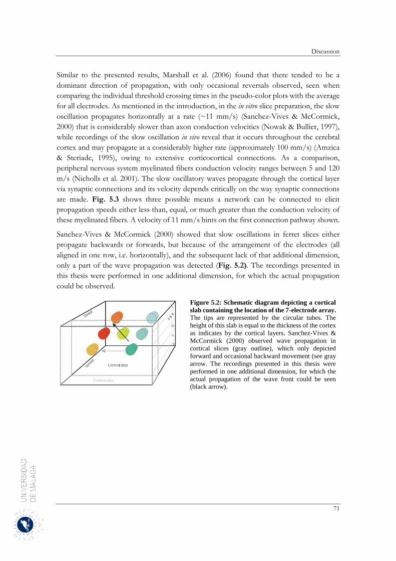
Discussion
71
Similar to the presented results, Marshall et al. (2006) found that there tended to be a
dominant direction of propagation, with only occasional reversals observed, seen when
comparing the individual threshold crossing times in the pseudo-color plots with the average
for all electrodes. As mentioned in the introduction, in the in vitro slice preparation, the slow
oscillation propagates horizontally at a rate (~11 mm/s) (Sanchez-Vives & McCormick,
2000) that is considerably slower than axon conduction velocities (Nowak & Bullier, 1997),
while recordings of the slow oscillation in vivo reveal that it occurs throughout the cerebral
cortex and may propagate at a considerably higher rate (approximately 100 mm/s) (Amzica
& Steriade, 1995), owing to extensive corticocortical connections. As a comparison,
peripheral nervous system myelinated fibers conduction velocity ranges between 5 and 120
m/s (Nicholls et al. 2001). The slow oscillatory waves propagate through the cortical layer
via synaptic connections and its velocity depends critically on the way synaptic connections
are made. Fig. 5.3 shows three possible means a network can be connected to elicit
propagation speeds either less than, equal, or much greater than the conduction velocity of
these myelinated fibers. A velocity of 11 mm/s hints on the first connection pathway shown.
Sanchez-Vives & McCormick (2000) showed that slow oscillations in ferret slices either
propagate backwards or forwards, but because of the arrangement of the electrodes (all
aligned in one row, i.e. horizontally), and the subsequent lack of that additional dimension,
only a part of the wave propagation was detected (Fig. 5.2). The recordings presented in
this thesis were performed in one additional dimension, for which the actual propagation
could be observed.
Figure 5.2: Schematic diagram depicting a cortical
slab containing the location of the 7-electrode array.
The tips are represented by the circular tubes. The
height of this slab is equal to the thickness of the cortex
as indicates by the cortical layers. Sanchez-Vives &
McCormick (2000) observed wave propagation in
cortical slices (gray outline), which only depicted
forward and occasional backward movement (see gray
arrow. The recordings presented in this thesis were
performed in one additional dimension, for which the
actual propagation of the wave front could be seen
(black arrow).
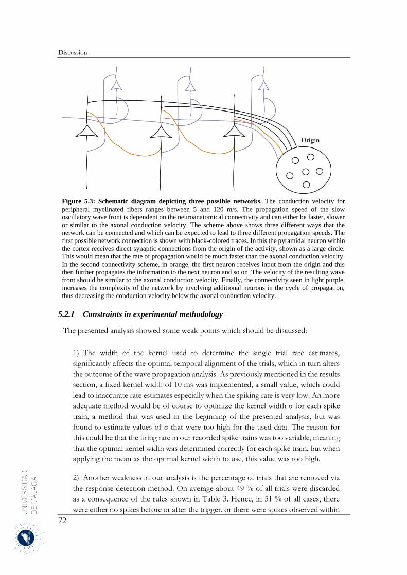
Discussion
72
Figure 5.3: Schematic diagram depicting three possible networks. The conduction velocity for
peripheral myelinated fibers ranges between 5 and 120 m/s. The propagation speed of the slow
oscillatory wave front is dependent on the neuroanatomical connectivity and can either be faster, slower
or similar to the axonal conduction velocity. The scheme above shows three different ways that the
network can be connected and which can be expected to lead to three different propagation speeds. The
first possible network connection is shown with black-colored traces. In this the pyramidal neuron within
the cortex receives direct synaptic connections from the origin of the activity, shown as a large circle.
This would mean that the rate of propagation would be much faster than the axonal conduction velocity.
In the second connectivity scheme, in orange, the first neuron receives input from the origin and this
then further propagates the information to the next neuron and so on. The velocity of the resulting wave
front should be similar to the axonal conduction velocity. Finally, the connectivity seen in light purple,
increases the complexity of the network by involving additional neurons in the cycle of propagation,
thus decreasing the conduction velocity below the axonal conduction velocity.
5.2.1 Constraints in experimental methodology
The presented analysis showed some weak points which should be discussed:
1) The width of the kernel used to determine the single trial rate estimates,
significantly affects the optimal temporal alignment of the trials, which in turn alters
the outcome of the wave propagation analysis. As previously mentioned in the results
section, a fixed kernel width of 10 ms was implemented, a small value, which could
lead to inaccurate rate estimates especially when the spiking rate is very low. An more
adequate method would be of course to optimize the kernel width σ for each spike
train, a method that was used in the beginning of the presented analysis, but was
found to estimate values of σ that were too high for the used data. The reason for
this could be that the firing rate in our recorded spike trains was too variable, meaning
that the optimal kernel width was determined correctly for each spike train, but when
applying the mean as the optimal kernel width to use, this value was too high.
2) Another weakness in our analysis is the percentage of trials that are removed via
the response detection method. On average about 49 % of all trials were discarded
as a consequence of the rules shown in Table 3. Hence, in 51 % of all cases, there
were either no spikes before or after the trigger, or there were spikes observed within
Discussion
73
the Down state. One way to possibly circumvent this problem could be to increase
the time interval used as a cut-out, so instead of 200 ms before and after the trigger,
300 ms might have been be a better value. But in the latter case, might create another
problem, i.e. detecting spikes belonging to the previous Up state, or even the
subsequent one. This is rather unlikely because our estimates of both the durations
of the Up and Down states show that both have a dwell time ranging between 360
and 480 ms.
3) The somatosensory cortex of the rat is located at 1.25 mm - 7.2 mm medial to
lateral and rostral to caudal from bregma 2.7 mm - bregma -4.52 mm. To consistently
record from the same location, these stereotactic coordinates should have been used.
In these experiments we made an estimated guess on the location. This inconsistency
means that there might have been differences in the location of the recording for
each session. If the variability in the spatio-temporal pattern observed in our 7-
electrode array recordings were only unique for that particular location of the
somatosensory cortex, it could mean that there are numerous focal points where this
activity is initiated; it then travels a certain distance (maybe up to 2 mm) and direction,
then tapers off. Thus, instead of there being one large activity wave spreading over
the cortex, there would be many different wave fronts, with their own characteristic
focal point and direction. It is very doubtful that the locations we recorded from were
that different, but if these smaller wave fronts overlapped, the overall vector
describing the activity wave would also change and result in findings similar to ours.
4) Furthermore, the intensity of the state transitions depended on the depth of the
anesthesia. We monitored this depth by checking sporadically for the pinch
withdrawal reflex as well as vibrissal movements. If required an additional dose of
ketamine-xylazine was administered. The timing between the injection and the start
of a recording session fluctuated, meaning that on some occasions it had been an
hour since the last injection, while on other occasions it had only been a few minutes.
The number of individual units detected by the extracellular array increased
dramatically in response to the administration of the ketamine-xylazine. This effect
wore off after some time and so some of our recordings may show more multi-unit
activity then others, again due to a lack of consistency in our experimental
procedures.
5) Due to the dimension and rigidity of the 7-electrode extracellular array, the slow
oscillatory activity might have been caused or altered because of tissue damage caused
by the array. Its insertion into the brain tissue required the initial removal of the dura.
This procedure did not entirely prevent the problem of dimpling, which occurred
because of the large surface area (~1.12 mm2) of the array pushing against the very
thin, but quite stabile pia. This dimpling effect gradually disappeared as the tissue
gave way to the continual pressure put on it by the array. Both the outer quartz mantle
and the metal core of the electrode fibers are tapering down to very small dimensions.
The passage between the glass isolation and the core of these electrode fibers is very
Discussion
74
smooth. The result is that there will be not so much tissue damage during electrode
penetration. Due to their smooth shape and their small dimensions, the used
microelectrodes cause only minimal tissue damage. In fact, tissue damage is so small
that electrode tracks could not be verified with standard histological techniques. With
this 7-electrode array, due to the alignment of the tips, it was only possible to position
it in one specific layer of the somatosensory cortex, thus parallel to the layering of
the cortex.
Discussion
75
6 Conclusions
1. In the somatosensory cortex of anesthetized rats and the visual cortex of anesthetized cats the
emergent slow oscillations were analyzed by means of intracellular and/or multiple extracellular
recordings.
2. A new algorithm for detection of slow waves, MAUDS (Moving Averages for Up and Down
Separation), a simple but robust method to detect cortical waves is described. MAUDS can be
applied in real time during the recording and also for offline processing of large amounts of
recorded data on conventional computers.
3. We tested and demonstrated that MAUDS efficiently separates Up and Down states in ideal as
well as in irregular oscillations for further analysis of cortical dynamics.
4. The stereotypical behavior of spontaneous transitions between the detected Up and Down states
in the somatosensory cortex of anesthetized rats is examined.
5. Waves of cortical activity under ketamine/xylazine anesthesia show considerable variability with
respect to their spatio-temporal pattern.
6. However, the results indicate that activity propagation in most animals showed a preferred
direction travelling in wave fronts across the cortex.
7. This suggests, that during slow wave sleep, activity waves may travel in a stereotypic manner over
the cortical tissues thereby sequentially activating neighboring cortical columns.
References
76
7 References
Abeles M, Bergman H, Margalit E, Vaadia E (1993) Spatiotemporal firing patterns in the frontal cortex of behaving monkeys. J Neurophysiol 70:1629–1638.
Achermann P, Borbely AA (1997) Low-frequency (< 1 Hz) oscillations in the human sleep electroencephalogram. Neuroscience 81: 213-222.
Amzica F, Steriade M (1995) Short- and long-range neuronal synchronization of the slow (< 1 Hz) cortical oscillation. J Neurophysiol 73: 20-38.
Amzica F, Steriade M (1997) The K-complex: its slow (<1-Hz) rhythmicity and relation to delta waves. Neurology 49: 952-959.
Anderson J, Lampl I, Reichova I, Carandini M, Ferster D (2000) Stimulus dependence of two-state fluctuations of membrane potential in cat visual cortex. Nat Neurosci 3: 617-621.
Arieli A, Sterkin A, Grinvald A, Aertsen A (1996) Dynamics of ongoing activity: Explanation of the large variability in evoked cortical responses. Science 273 (5283): 1868-1871.
Ascoli GA, Alonso-Nanclares L, Anderson SA, Barrionuevo G, Benavides-Piccione R, Burkhalter A, …& Yuste R (2008) Petilla terminology: nomenclature of features of GABAergic interneurons of the cerebral cortex. Nat Rev Neurosci 9:557–68.
Azouz R, Gray CM (1999) Cellular mechanisms contributing to response variability of cortical neurons in vivo. J Neurosci 19: 2209-2223.
Bal T, von Krosigk M, McCormick DA (1995) Synaptic and membrane
mechanisms underlying synchronized oscillations in the ferret lateral geniculate nucleus
in vitro. J Physiol 483:641-663
Barth DS, MacDonald KD (1996) Thalamic modulation of high-frequency oscillating potentials in auditory cortex. Nature 383:78-81.
Bazhenov M, Timofeev I, Steriade M, Sejnowski TJ (2002) Model of thalamocor- tical slow-wave sleep oscillations and transitions to activated states. J Neurosci 22: 8691–8704.
Braak H, Braak E (1984) Neuronal types in the neocortex-dependent lateral territory of the human thalamus. A Golgi-pigment study. Anat Embryol (Berl) 169(1):61-72.
Blethyn KL, Hughes SW, Tóth TI, Cope DW, Crunelli V (2006) Neuronal basis of the slow (1 Hz) oscillation in neurons of the nucleus reticularis thalami in vitro. J Neurosci 26: 2474–2486.
Benucci A, Verschure PF, Konig P (2004) Two-state membrane potential fluctuations driven by weak pairwise correlations. Neural Comput 16: 2351-2378.
Berger H (1929) On the electroencephalogramm of man. Archiv.Psychiatrische Nervenkrankheiten 87:527-520.
Berlin R (1858) Beiträge zur Struktur der Grosshirnwindungen. Erlangen.
Brodmann K (1908) Beiträge zur histologischen Lokalisation der Grosshirnrinde, die Cortexgliederung des Menschen. J Pychol Neurol 231
Brodmann K (1912) Neue Ergebnisse über die vergleichende histologische
References
77
Lokalisation der Grosshirnrinde mit besonderer Berücksichtigung des Stirnhirns. Anat Anz Suppl 41:157-216.
Brodmann K (1914) Physiologie des Gehirns. In Neue Deutsche Chirurgie. Vol IX, ed. P.v. Brun, 85-462. Stuttgart.
Buzsáki G, Draguhn A (2004) Neuronal oscillations in cortical networks. Science 304: 1926-1929
Chagnac-Amitai Y, Connors BW (1989) Horizontal spread of synchronized activity in neocortex and its control by GABA-mediated inhibition. J Neurophysiol 61: 747-758
Chauvette S, Volgushev M, Timofeev I (2010) Origin of active states in local neocortical networks during slow sleep oscillation. Cereb Cortex 20: 2660– 2674, 2010.
Compte A, Sanchez-Vives MV, McCormick DA, Wang XJ (2003) Cellular and network mechanisms of slow oscillatory activity (<1Hz) and wave propagations in a cortical network model. J Neurophysiol 89:2707-2725.
Contreras D, Steriade M. (1997) State-dependent fluctuations of low-frequency rhythms in corticothalamic networks. Neuroscience 76:25-38.
Contreras D, Steriade M. (1995) Cellular basis of EEG slow rhythms: a study of
dynamic corticothalamic relationships. J Neurosci 15: 604–622.
Cowan RL, Wilson CJ (1994) Spontaneous firing patterns and axonal projections of single corticostriatal neurons in the rat medial agranular cortex. J Neurophysiol 71: 17-32.
Crochet S, Chauvette S, Boucetta S, Timofeev I (2005) Modulation of synaptic transmission in neocortex by network activities. Eur J Neurosci 21: 1030-1044.
Crochet S, Fuentealba P, Timofeev I, Steriade M (2004) Selective amplification of neocortical neuronal output by fast prepotentials in vivo. Cereb Cortex 14: 1110-1121.
Curro-Dossi R, Nuñez A, Steriade M (1992) Electrophysiology of a slow (0.5-4Hz) intrinsic oscillation of cat thalamocortical neurons in vivo. J Physiol 447:215-34.
Danneman, P.J. (1995) Preoperative, Intra-operative, and Post-operative Care of Rabbits and Rats with Emphasis on Anesthesia and Analgesia. Oral Presentation and Proceedings of the 1995 Michigan Veterinary Conference, pp 107-114
Diesmann M, Gewaltig MO, and Aertsen A (1999) Conditions for Stable Propagation of Synchronous Spiking in Cortical Neural Networks. Nature 402:529-533.
Ellinger AG (1971) The art of investment. London: Bowes and Bowes.
Ferezou I, Bolea S, Petersen CC. (2006) Visualizing the cortical representation of
whisker touch: voltage-sensitive dye imaging in freely moving mice. Neuron 50: 617–629.
Fontanini A, Spano PF, Bower JM (2003) Ketamine-xylazine-induced slow (~1.5 Hz) oscillations in the rat piriform (olfactory) cortex are functionally correlated with respiration. J Neurosci 23: 7993–8001.
Fucke T, Suchanek D, Nawrot MP, Seamari Y, Heck DH, Aertsen A, Boucsein C (2011) Stereotypical spatiotemporal activity patterns during slow-wave activity in the neocortex, J Neurophysiol 106: 3035-3044.
Fuentealba P, Steriade M (2005) Thalamic oscillations modulate membrane properties of cat thalamic reticular neurons. Thal Rel Syst 3: 53-62.

References
78
Gennari F (1782) De peculiari structura cerebri nonnulisque eius morbis. Parma.
Golgi C (1873) Sulla struttura della sostanza grigia del cervello. Gazz Med Lombarda 33:244-246.
Golgi C (1883) Recherches sur l’histologie des centres nerveux. Arch Italiennes de Biol 3:285-317.
Haider B, Duque A, Hasenstaub AR, McCormick DA (2006) Neocortical network activity in vivo is generated through a dynamic balance of excitation and inhibition. J Neurosci 26: 4535-4545.
Hara K, Harris RA (2002) The anesthetic mechanism of urethane: the effects on neurotransmitter-gated ion channels. Anesth Analg 94: 313-8
Holcman D, Tsodyks M (2006) The emergence of up and down states in cortical networks. PLoS Comput Biol 2: e23.
Hubel DH, Wiesel TN (1959) Receptive fields of single neurons in the cats striate cortex. J Physiol 148(3):574-591.
Kandel ER, Schwartz JH, Jessell TM (2000) Principles of Neural Science 4th ed. McGraw-Hill, New York. ISBN 0-8385-7701-6
Kasanetz F, Riquelme LA, Murer MG (2002) Disruption of the two-state membrane potential of striatal neurones during cortical desynchronisation in anesthetised rats. J Physiol 543: 577-589.
Kisvarday ZF, Martin KAC, Freund TF, Magloczky ZS, Whitteridge D and Somogyi P (1986) Synaptic targets of HRP-filled layer III pyramid cells in the striate cortex. Exp Brain Res 44:541-552.
König P, Engel AK, Singer W (1996) Integrator or coincidence detector? The role of the cortical neuron revisited. Trends in Neurosciences 19:130–137.
Krosigk von M., Bal T., McCormick DA (1993) Cellular mechanisms of a synchronized oscillation in the thalamus. Science 261 (5119): 361-364.
Lampl I, Reichova I, Ferster D (1999) Synchronous membrane potential fluctuations in neurons of the cat visual cortex. Neuron 22: 361-374.
Larkman AU (1991) Dendritic morphology of pyramidal neurones of the visual cortex of the rat: III. Spine distributions. J Comparative Neurology, 306 (2): 332-343.
Leresche N, Lightowler S, Soltesz I, Jassik-Gerschenfeld D, Crunelli V (1991) J Physiol 441:155-174.
Lewis BL, O'Donnell P (2000) Ventral tegmental area afferents to the prefrontal cortex maintain membrane potential 'up' states in pyramidal neurons via D(1) dopamine receptors. Cereb Cortex 10: 1168-1175.
MacDonald JF, Bartlett MC, Mody I, Pahapill P, Reynolds JN, Salter MW, Schneiderman JH, Pennefather PS. (1991) Actions of Ketamine, phencyclidine and MK-801 on NMDA receptor currents in cultured mouse hippocampal neurones. J Physiol (London) 432:483-508.
Mahon S, Deniau JM, Charpier S (2003) Various synaptic activities and firing patterns in cortico-striatal and striatal neurons in vivo. J Physiol Paris 97: 557-566.
Mahon S, Deniau JM, Charpier S (2001) Relationship between EEG potentials and intracellular activity of striatal and cortico-striatal neurons: An in vivo study under

References
79
different anesthetics. Cereb Cortex 11: 360-373.
Martin KAC & Whitteridge D (1984) Form, function and intracortical projections of spiny neurones in the striate visual cotex of the cat. J Physiol 353:463-504.
Marshall L, Helgadóttir H, Mölle M, & Born J (2006) Boosting slow oscillations during sleep potentiates memory. Nature 444: 610-613
Massimini M, Huber R, Ferrarelli F, Hill S, Tononi G (2004) The sleep slow oscillation as a traveling wave. J Neurosci 24: 6862-6870.
Massimini M, Amzica F. (2001) Extracellular calcium fluctuations and intracellular potentials in the cortex during the slow sleep oscillation. J Neurophysiol 85: 1346 –1350.
Mattia M. & Sanchez-Vives MV (2012) Exploring the spectrum of dynamical regimes and timescales in spontaneous cortical activity. Cogn Neurodyn 6(3): 239-250.
MacDonald JF, Bartlett MC, Mody I, Pahapill P, Reynolds JN, Salter MW, Schneiderman JH, Pennefather PS. (1991) Actions of ketamine, phencyclidine and MK-801 on NMDA receptor currents in cultured mouse hippocampal neurones. J Physiol 432: 483–508.
McCormick DA, Pape HC (1990) Properties of a hyperpolarization-activated cation current and its role in rhythmic oscillation in thalamic relay neurones. J Physiol 431:291-318.
McCormick DA, Shu Y, Hasenstaub A, Sanchez-Vives M, Badoual M, Bal T (2003) Persistent cortical activity: mechanisms of generation and effects on neuronal excitability. Cereb Cortex 13: 1219-1231.
Metherate R, Ashe JH (1993) Ionic flux contributions to neocortical slow waves and nucleus basalis mediated activation - whole-cell recordings in-vivo. J Neurosci 13: 5312-5323.
Mukovski M, Chauvette S, Timofeev I, Volgushev M (2007) Detection of active and silent states in neocortical neurons from the field potential signal during slow-wave sleep. Cereb Cortex 17: 400-414.
Nawrot MP, Aertsen A, Rotter S. (2003) Elimination of response latency variability in neuronal spike trains. Biol Cybern 88:321-334.
Nicholls J, Martin AR, Fuchs PA, Brown DA, Diamond M, Weisblat DA (2001) From Neuron to Brain. ISBN: 978-0-87893-609-0
Nicoll RA, Malenka RC, Kauer JA (1990) Functional comparison of neurotransmitter receptor subtypes in mammalian central nervous system. Phys Rev 70: 513-565.
Nowak LG, Bullier J (1997) in Cerebral Cortex: Extrastriate Cortex in Primates Vol.12 (eds. Rockland K, Kaas JH, Peters A) 205-241 (Plenum, New York).
Nowak LG., Azouz R, Sanchez-Vives MV, Gray CM, McCormick DA (2003) Electrophysiological classes of cat primary visual cortical neurons in vivo as revealed by quantitative analyses. J Neurophysiol 89:1541–1566, 10.1152/jn.00580.2002
Peters Y, Barnhardt NE, O'Donnell P (2004) Prefrontal cortical up states are synchronized with ventral tegmental area activity. Synapse 52: 143-152.
Petersen C, Hahn T, Mehta M, Grinvald A, Sakmann B (2003) Interaction of sensory responses with spontaneous depolarization in layer 2/3 barrel cortex. Proc Natl Acad

References
80
Sci U S A 100: 13638-13643.
Ramón y Cajal S (1899) Estudio sobre la corteza cerebral humana. Rev Trimest Microscopia 4:1-63.
Rechtschaffen A, Kales A (1968) A manual of standardized terminology, techniques and scoring system for sleep stages of human subjects. Washington, DC: National Institutes of Health.
Reig R, Zerlaut Y, Vergara R, Destexhe A, Sanchez-Vives MV (2015). Gain modulation of synaptic inputs by network state in auditory cortex in vivo. J Neurosc 35: 2689-2702.
Reig R & Sanchez-Vives, MV (2007) Synaptic transmission and plasticity in an active cortical network. PLoS One 2:e670-e670.
Riedner BA, Vyazovskiy VV, Huber R, Massimini M, Esser S, Murphy M, Tononi G (2007) Sleep homeostasis and cortical synchronization: III. A high-density EEG study of sleep slow waves in humans. Sleep 30:1643-1657.
Rubino D, Robbins KA, Hatsopoulos NG (2006) Propagating waves mediate information transfer in the motor cortex. Nat Neurosci 9:1549-1557.
Ruiz-Mejias M, Ciria-Suarez L, Mattia M, Sanchez-Vives M. V (2011) Slow and fast rhythms generated in the cerebral cortex of the anesthetized mouse. J Neurophysiol 106: 2910-2921
Sachdev RN, Ebner FF, Wilson CJ (2004) Effect of subthreshold up and down states on the whisker-evoked response in somatosensory cortex. J Neurophysiol 92: 3511-3521.
Sakata S, Harris KD (2009) Laminar structure of spontaneous and sensory-evoked
population activity in auditory cortex. Neuron 64:404-418.
Sanchez-Vives MV, McCormick DA (2000) Cellular and network mechanisms of rhythmic recurrent activity in neocortex. Nat Neurosci 3: 1027-1034.
Scheibel ME, Scheibel AB (1958) Structural substrates for integrative patterns in the brain stm reticular core. Little Brown, Boston 33-55.
Seamari Y, Narvaez JA, Vico FJ, Lobo D, Sanchez-Vives MV (2007) Robust off- and online separation of intracellularly recorded Up and Down cortical states. PLoS ONE 2(9): e888
Sharma AV, Wolansky T, Dickson CT (2010) A comparison of sleeplike slow oscillations in the hippocampus under ketamine and urethane anesthesia. J Neurophysiol 104: 932–939.
Shu Y, Hasenstaub A, Badoual M, Bal T, McCormick DA. (2003) Barrages of synaptic activity control the gain and sensitivity of cortical neurons. (J Neurosci) 23:10388–10401.
Simon NR, Manshanden I, Lopes da Silva FH (2000) A MEG study of sleep. Brain Res 860: 64-76.
Soemmering ST (1788). Vom Hirn und Rückenmark. Mainz.
Steriade M (1996) Awakening the brain. Nature 383:24-25.
Steriade M (1997) Slow sleep oscillation, rhythmic K-complexes, and their paroxysmal developments. J Sleep Res 7:30-35.
References
81
Steriade M, Dossi RC, Nunez A (1991) Network modulation of a slow intrinsic oscillation of cat thalamocortical neurons implicated in sleep delta waves: Cortically induced synchronization and brainstem cholinergic suppression. J Neurosci 11: 3200-3217.
Steriade M, Amzica F, Contreras D (1996) Synchronization of fast (30-40 Hz) spontaneous cortical rhythms during brain activation. J Neurosci 16: 392-417.
Steriade M, McCormick DA, Sejnowski TJ (1993) Thalamocortical oscillations in the sleeping and aroused brain. Science 262:679-685.
Steriade M, Nunez A, Amzica F (1993a) A novel slow (< 1 Hz) oscillation of neocortical neurons in vivo: depolarizing and hyperpolarizing components. J Neurosci 13: 3252-3265.
Steriade M, Nunez A, Amzica F (1993b) Intracellular analysis of relations between the slow (< 1 Hz) neocortical oscillation and other sleep rhythms of the electroencephalogram. J Neurosci 13: 3266-3283.
Steriade M (2000) Corticothalamic resonance, states of vigilance and mentation. Neurosci 101(2): 243-276.
Steriade M, Timofeev I, Grenier F (2001) Natural waking and sleep states: a view from inside neorcortical neurons. J Neurophysiol 85:1969-1985.
Stern EA, Kincaid AE, Wilson CJ (1997) Spontaneous subthreshold membrane potential fluctuations and action potential variability of rat corticostriatal and striatal neurons in vivo. J Neurophysiol 77: 1697-1715.
Stickgold R, Walker MP (2005) Memory consolidation and reconsolidation: what is the role of sleep? Trends Neurosc 28:408-415
Stroh A, Adelsberger H, Groh A, Rühlmann C, Fischer S, Schierloh A, ... & Konnerth A (2013) Making waves: initiation and propagation of corticothalamic Ca 2+ waves in vivo. Neuron 77: 1136-1150.
Takagaki K, Zhang C, Wu JY, Lippert MT (2008) Crossmodal propagation of
sensory-evoked and spontaneous activity in the rat neocortex. Neurosci Lett 431: 191–196.
Timofeev I, Contreras D, Steriade M (1996) Synaptic responsiveness of cortical and thalamic neurones during various phases of slow sleep oscillation in cat. Journal of Physiology-London 494: 265-278.
Timofeev I, Grenier F, Bazhenov M, Sejnowski TJ, Steriade M (2000) Origin of slow cortical oscillations in deafferented cortical slabs. Cereb Cortex 10: 1185-1199.
Timofeev I, Grenier F, Steriade M (2001) Disfacilitation and active inhibition in the neocortex during the natural sleep-wake cycle: an intracellular study. Proc Natl Acad Sci U S A 98: 1924-1929.
Tseng KY, Kasanetz F, Kargieman L, Riquelme LA, Murer MG (2001) Cortical slow oscillatory activity is reflected in the membrane potential and spike trains of striatal neurons in rats with chronic nigrostriatal lesions. J Neurosci 21: 6430-6439.
Tsodyks M, Kenet T, Grinvald A, Arieli A (1999) Linking spontaneous activity of single cortical neurons and the underlying functional architecture. Science 286 (5446): 1943-1946.
Vicq d’Azyr F (1786) Traité d’anatomie et de physiologie. Paris.
References
82
Villablanca J (1974) Role of the thalamus in sep control: Sleep-wakefullness studies in chronic diencephalic and athalamic cats. In Petre-Quadens O, Schlag JD, eds. Basic sleep mechanisms. New York: Academic Press, p. 51-78
Volgushev M, Chauvette S, Mukovski M, Timofeev I (2006) Precise long-range synchronization of activity and silence in neocortical neurons during slow-wave oscillations [corrected]. J Neurosci 26: 5665-5672.
Waters J, Helmchen F (2006) Background synaptic activity is sparse in neocortex. J Neurosci 26: 8267–8277, 2006.
Wilson C, Kawaguchi Y (1996) The origins of two-state spontaneous membrane potential fluctuations of neostriatal spiny neurons. J Neurosci 16: 2397-2410.
Xu W, Huang X, Takagaki K, Wu JY (2007) Compression and reflection of visually evoked cortical waves. Neuron 55: 119–129.

Appendix
83
8 Appendix
8.1 Protocol for in vivo experiments
- Switch on the heating pad, prepare surgery place and tools which were all previously sterilized.
- Prepare fresh Urethane 20% (2 mg Urethane in 8ml NaCl 0.9%). Urethane is highly carcinogenic, therefore handle with care and wear the impermeable nitrile gloves.
- Pick up the rat from the animal facilities.
- Weight the rat in order to determine the injection amount of Urethane.
- Inject the rat with Urethane 20% i.p (0.5 ml/100 g body weight) helping yourself with the slipper to fix the rat, cover the rat cage, dim the lights, wait at least ½ hour till the rat is anesthetized.
- During that standby time: preparation of Ketamine/Xylazine mixture, Lidocaine, potassium acetate 1M, filter it. Get prepared the razor.
- Check status of anesthesia: Rat is moving when trying to touch it? Whiskering? Blinking? Rat’s hindlimb withdrawal reflex is still present?
- If yes: Reinject with 10% initial Urethane dose and wait circa further 15 minutes, check again the status.
- If no: Reinject with 0.1 ml Ket/Xyl.
- Shave the head fur for the surgery. Shave also the left hindlimb and both forelimbs to assure contact between ECG electrodes and rat skin. Place the rat on the heating pad to avoid hypothermia.
- Place the earbars correctly and fix the rat into the stereotaxic apparatus. Check if you got the right position: when you insert the earbar into the ear, you may be able to observe a blink reflex of the eye of the same side. You may also hear cracking the Membrana tympani. The head should be in a straight position and the ears should form a line. You must be able to move the head of the rat in the vertical direction, but when you stop moving the head should stay in the same position. There should be no movement in the horizontal direction at all.
- Get stuck the incisors of the rat into the incisors bar of the stereotaxic device and fixate the nose holder attaching closely, but take care not to injure the rat.
- Lubricate the thermometer with a fatty ointment (Vaseline ) and insert it carefully into the rectum. Note down the temperature which should be around 37ºC without exceeding 39ºC.
- Connect the ECG electrodes to the limbs and view it on the screen (there will be noise until you place the reference electrode in the neck).
- Cover the rat with a towel in order to prevent hypothermia.
- Apply eye ointment to protect the cornea (Bepanthen ) against drying and apply Betadine on the shaved area of the head with a generously soaked pad.
- Inject Lidocaine s.c. where you will make the incision of the skin. Disperse it evenly juddering the skin softly with your finger.
- Place the scalpel onto the skull, frontal, close to the beginning of the midline and applying a certain pressure separate the skin with a single incision until the end of head bone.
- Lay open the bone by separating the skull with the hooks. Clean away fatty tissue and musculature. Scratch off carefully the periosteum using the most appropriate tool for it (with the aid of the binocular Zeiss OPMI 1). Clean the bone every once a while with a cotton swab, saline soaked if needed.
Appendix
84
- Open a way to the Cisterna magna by twitching off carefully the muscles and the connective tissue with a blunt tool. Separate with the same blunt tool or with the blunt tweezers the skin from the underlying connective tissue in order to have enough space to insert the reference electrode into the neck.
- Find bregma and mark with a waterproof pencil on the bone where to drill the hole for the fixation screw and where to drill the window for recording. intracellular window is missing
- Inject 2ml NaCl s.c. into the back of the rat (“give it to drink”) in order to avoid dehydration.
- Check once in a while the deepness of anesthesia of the rat. If the rat whiskers (or even blinks) then it’s time to inject 0.1 ml to 0.2 ml Ket/Xyl. i.p.
- Drill carefully the hole for the fixation screw under binocular. Use the drill head size 10 and the the highest magnification – it is very easy to pop into the Dura. Fixate the screw using as a holder the bent tweezers and the clockmaker screw driver.
- Start drilling carefully into the skull bone the window for recording. First mark the opening by drilling a groove following the pencil mark. Continue drilling deeper and deeper but uniformly until you can appreciate the tissue and vessels below the bone. Clean off the bone splits for a better sight by blowing with for instance with an empty Pasteur pipette. The bone window should be loose, such that it should be removable applying soft forces upwards with the tweezers (but don’t remove it yet!).
- As there are also vessels within the bone, bleeding during drilling is frequent. These might make difficult visibility and therefore slow down the whole drilling process. In such cases: clean off the blood applying NaCl 0.9% with a syringe and wiping softly with a Q-tip, or when you’re sure to be still far away from the brain tissue, then, since sometimes it just stops, continue drilling even of the bleeding (the drilling cauterizes the bleeding). If this does not help you can use the soldering gun (temperature 250°C) and tip carefully on the bleeding side to cauterize the vessel. Note that drilling quickly and efficiently the hole is better than a slow hole since it minimizes edema.
- Build up the funnel with the dental acryl cement taking care that no liquid acryl cement flows into the hole. Check that the funnel does not leak saline. Let it dry.
- Mount both micromanipulators, and check their positioning: must be perpendicular one to the other. Check the range of the vertical arm of the micromanipulator.
- Remove the bone flap with fine forceps. Very carefully nick the Dura mater with the keenest (finest?) hypodermic needle (at least 30 Gauge or smaller). Always take a new needle. If the incision is complete, liquor will flow. Use the eye scissors to lift the dura and cut carefully to extend the hole. Use maximum precaution not to damage blood vessels nor the cortical surface. Note that the dura is laminar and often one thin sheet of the dura remains, even though it looks as if the dura is completely removed. In older animals, the dura is fat and whitish, therefore easy to distinguish. Quickly add saline (HEPES-buffered ACSF to prevent pH shifts) to keep surface moist.
- Fix the Multielectrode-Array into the micromanipulator and advance into the tissue. Try to avoid the blood vessels because electrodes cannot pass through them and this produces a higher dimpling.
Conditions to start a recording session:
- The multielectrode-array is placed within the cortex and there is good spontaneous activity on all electrodes
- The intracellular recorded neuron exhibits a stable Vm ≤ -55mV, stable electrophysiological properties without the use of “retaining” i.e. hyperpolarizing current and the ability to generate repetitive APs in response to depolarizing current pulses (additionally to determine “off line”: input resistance >20MOhm).
- Spontaneous activity: Simultaneous extra- and intracellular recordings

Appendix
85
- Bridge compensation within the cell: asymmetric pulses of 0.1nA amplitude an 2ms duration.
- Subthreshold activity: Injection of hyperpolarizing current into the intracellularly recorded neuron. Increase negative I until the neuron stops to spike.
- Asymmetric hyperpolarizing current pulses, 0.2nA amplitude and 200ms duration.
- Asymmetric depolarizing current pulses, 0.2nA amplitude and 200ms duration.
- Filling of the neuron with Neurobiotin® Dye applying I = +1nA, 200ms pulses during min. 10 minutes.
- Check the offset after pulling the electrode out of the tissue, but still within the solution.
- Draw or take a photo from the brain surface to determine roughly the position of the recorded neuron during the staining. Urethane Injection:
- 2g Urethane + 8ml of NaCl (20%)-
- Place in plastic tube with blue cap and shake to dissolve.- Inject 0.5ml per 100 g body weight i.p. Use 26 gage needle and 10ml syringe. Needs approximately 30 min to take effect, whiskers can still be present, but animal should be anesthetic for pain stimulus. Saline solution: NaCl 0.9% solution.
- 100ml use 0.90g of NaCl.Place in small bottle, label and fill a syringe with this. Ketamine / Xylazine: 10% Ketamine ® 1ml using syringe
- 1% Xylocain (Rompun®) 0.5ml using syringe
- Add together and mix in Eppendorf® tube. Inject 0.1 ml i.p. in each time interval until the complete anesthesia. Potassium acetate (KC2H3O3) 1M:
- For 10 ml of distilled water use 0.98 g of potassium acetate.
- Place in plastic test tube with blue cap and label.
- Neurobiotin: Disolve 8mg of Neurobiotin® in 400ml filtered potassium acetate 1M solution and place in a 1ml syringe with filter (0.2um)
- Local anesthetic: Fill 0.5 ml Lidocain® in syringe and label Paraformaldehyde (PFA) 4%
- The whole preparation has to be done under the extraction hood, and use reserved and marked tools only, because of the high toxicity of PFA.
- For 1 l PB 0.1 M, +4ºC, pH 7.4
- Add 10 mg PFA to 950 ml Aqua dest. and stir with the aid of a magnetic stirrer
- Heat till 60ºC controlling the temperature with a thermometer
- Continue stirring and dissolve completely of PFA within the PB
- The dissolution can be stored in 500 ml after turning cold plastic bottles in the freezer. Phosphate Buffer 0.1M, pH 7.4
- For 1l add NaH2PO4 2,62 g to 950ml Aqua dest.
- Stir to dissolve and add Aqua dest. to complete 1 l
- Calibrate pH to 7.4 or
- Add Na2H PO4 14,42 g to 950 ml Aqua dest.
- Stir to dissolve and complete 1 l adding Aqua dest.
- Calibrate pH 7.4

Appendix
86
Chrome/Alum-Gelatin-coated slides
- For 500 ml Chrome/Alum Gelatin solution 0.5%
- Add 2.5 g Gelatin powder to 500 ml Millipore filtered distilled water
- Heat the water to 60 ºC and completely dissolve the gelatin with the aid of a magnetic stirrer. Do not exceed this temperature.
- Stir in 0.25 g chromium potassium sulfate (The solution should turn a pale blue). Add a few crystals of thymol as a preservative.
- Filter the Chrome/Alum-Gelatin dissolution twice
- Procedure:
- Dip racks of clean slides in the warm gelatin solution (40-50 ºC), drain the slides onto paper tissue, and then stand the slides (covered with foil to keep off dust) on end to air dry or 37 ºC incubator overnight.
- Store in dust-free container at room temperature. Throw out the gelatin mixture after use. DAB Reaction for free-floating sections
- Prerequisite: 6 slices / each 100 µm thick, been in 0.1M PB at least 24 hours.
- Chemicals/Materials: PBS 0.1M, pH 7.4
- Incubation chamber (flexible PVC, wells with slanted side walls, covered with plastic
- Triton X-100
- H2O2 30% (fresh)
- A and B solutions (Vectastain ABC-kit) Procedure - Day 1
- Quenching endogenous peroxidase
- Wash free floating slices in 0.1M PB about 2 times
- Prepare peroxidase 2% (2ml H2O2 + 28ml 0.1M PB) in 50 ml graduate cylinder and cover top with parafilm and carefully shake.
- Remove PB from each of the wells and add about 4 ml of the H2O2 2% to each well.
- Incubate during 60 minutes.
- Rinsing
- Remove the H2O2 and rinse with 0.1M PB 6-8 times 10 minutes, so that no more air bubbles appear on the slices.
- Biotin-avidin-complex
- During last 2-3 rinsing steps prepare the ABC reaction solution (2.5 ml per well):
- Use a 25 ml graduate cylinder and add 15 ml 0.1M PB.
- Using micropipette measure 150 µl A solution, 150 µl B solution, and 150 µl l of 10% Triton X (preparation of 100 ml 10% Triton X loading solution: 10 ml Triton X-100100% + 90 ml 0.1 M PB; loading solution storage in the fridge only for short time periods).
- Add parafilm to top and shake really well, may start to foam.
- Place in fridge for 30 minutes.
- Remove the PB from the last rinsing step.
- Add 2.5 ml ABC solution in each well
- Place the well plate onto the shaker and allow gentle agitation overnight. Day 2
- Before starting anything, check and prepare all the materials needed.
- Prepare everything that is needed under the extraction hood, this is very important because DAB is highly toxic (cancerigenic) and precautions need to be taken for its appropriate disposal:
Appendix
87
- Wear impermeable nitril gloves.
- Place heater/stirrer under the hood
- Use a separate and labeled beaker, into this the DAB rests and any substances that have come in contact with it will be disposed of. Add a small amount of sodium hypochlorite (stored in freezer) to neutralize the wrappers the DAB tablet were in.
- Prepare a small bottle and wrap in aluminium foil or similar which will later be used to filter the DAB solution into.
- Get funnel and filter paper ready.
- Set up a bottle to hold the brushes and the Pasteur pipette. Prepare the DAB solution
- Measure 30ml of Tris buffer pH 8.2 and place in small beaker.
- Stir with the aid of a magnetic stirrer.
- Get prepared the beaker with the aluminium foil around it, because the dissolving of the DAB tablets needs to be done in the dark.
- Open carefully the wrapper of 2 DAB tablets and place into beaker with Tris buffer.
- Place the beaker covered with aluminium foil over this and turn on the sitrrer.
- Remove the ABC solution from the (6) wells and subsequently rinse 6x3minutes the slices using 0.1M PB.
- Prior to the last rinsing step, filter the DAB solution with the aid of the funnel and allow to drip for a few minutes.
- Place the funnel into the labeled beaker and neutralize the funnel and the filter paper using sodium hypochlorite.
- Remove the PB form the slices as good as possible.
- Under hood, place first 1 ml of DAB into each well and then add 3ml more. Cover and place into the fridge for 25 minutes.
In the mean time:
- Calculate the amount of DAB needed:
- Considering 4ml of DAB per well: 4*3.3 µl 0.3% H2O2 per ml of DAB = 13.2µl in Eppendorf (990µl 0.1M PB + 10 µl 30% H2O2) 4*20 µl 10% NiCl per ml of DAB = 80 µl in Eppendorf
- Place these tubes under hood and prepare pipettes and pipette tips.
- Take the well plate out of fridge and place under the hood.
- Repeat the following steps for each of the (6) wells:
- Place 8 µl of NiCl into the well using micropipette (always dispose of the used tip into the labeled garbage beaker)
- Add 13.2 µl of H2O2 well.
- Mix the solution within the well carefully with the aid of a Pasteur pipette.
- Using the Pasteur pipette place a small amount into indentation of microscope slide.
- Help with a brush to place one slice and view under the microscope to check if the neuronal tissue is adequately stained.
- If not, place the slice back into the well to continue the DAB reaction.
- If it’s so, then stop the DAB reaction placing the slice with the aid of a brush into a new well plate with 0.1 M PB.
- Repeat for all slices.

Appendix
88
Dehydration
- Rinse the slices with 0.1MPB 3-4x10 minutes. Transfer the slice gently with the aid of a small brush from the well to the Gelatin coated slide and help to place the slice flat on it. With a paper tissue dry as far as possible without injuring the slice.
- Dehydrate the slices moving through series of increasing ethanol concentration starting with 60%, 70%, 80%, 90%, 100% during 2 minutes each.
- Transfer all slides into methyl benzoate overnight.
- Take out all the slides and let them laid under the hood until they loose the strong exhalation of the methyl benzoate.
- Covering the slides
- Put just one small drop of Mowiol onto the tissue on the slide and cover. Let them dry. Mowiol is not for permanent preparations, the tissue starts to bleach out after a few couple of months. Therefore, it’s important to reconstruct the stained neuron with the aid of a Camera Translucida.

Appendix
89
8.2 MAUDS Programming Scripts
Spike2 Script Version: In this version, the algorithm is written totally in the script language
of spike2. The advantage is the legibility of the code. The algorithm is executed in the pc,
sharing its resources with the task of recording the signals. So the delay of the characterization
and real-time triggering depends on the pc used.
http://geb.uma.es/images/projects/MAUDS/maudsScript.s2s
Spike2 Sequencer Version: In this version, the algorithm is implemented and executed into
the sequencer of the data acquisition unit. The response time of this solution is very high and
independent of the pc used. However, the code is much more illegible because it is written in
the assembler language of the sequencer.
http://geb.uma.es/images/projects/MAUDS/maudsSequencer.s2s
MATLAB® Version: Mauds implementation in MATLAB®. It can process mat data files
and Spike2 txt exported files. It does include plotting utilities.
http://geb.uma.es/images/projects/MAUDS/mauds4matlab.zip

Appendix
90
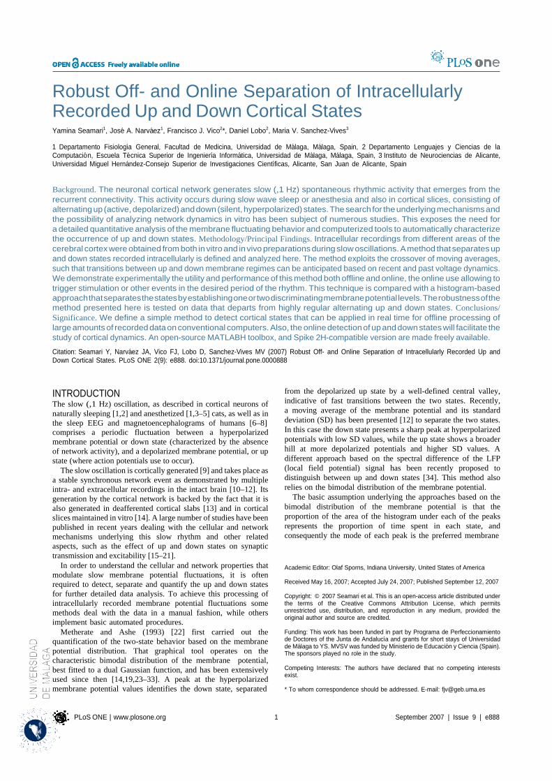
PLoS ONE | www.plosone.org 1 September 2007 | Issue 9 | e888
Robust Off- and Online Separation of Intracellularly Recorded Up and Down Cortical States
Yamina Seamari1, Jose A. Narva ez1, Francisco J. Vico2*, Daniel Lobo2, Maria V. Sanchez-Vives3
1 Departamento Fisiologıa General, Facultad de Medicina, Universidad de Malaga, Malaga, Spain, 2 Departamento Lenguajes y Ciencias de la Computacio n, Escuela Te cnica Superior de Ingenierıa Informatica, Universidad de Malaga, Malaga, Spain, 3 Instituto de Neurociencias de Alicante, Universidad Miguel Hernandez-Consejo Superior de Investigaciones Cientıficas, Alicante, San Juan de Alicante, Spain
Background. The neuronal cortical network generates slow (,1 Hz) spontaneous rhythmic activity that emerges from the recurrent connectivity. This activity occurs during slow wave sleep or anesthesia and also in cortical slices, consisting of alternating up (active, depolarized) and down (silent, hyperpolarized) states. The search for the underlying mechanisms and the possibility of analyzing network dynamics in vitro has been subject of numerous studies. This exposes the need for a detailed quantitative analysis of the membrane fluctuating behavior and computerized tools to automatically characterize the occurrence of up and down states. Methodology/Principal Findings. Intracellular recordings from different areas of the cerebral cortex were obtained from both in vitro and in vivo preparations during slow oscillations. A method that separates up and down states recorded intracellularly is defined and analyzed here. The method exploits the crossover of moving averages, such that transitions between up and down membrane regimes can be anticipated based on recent and past voltage dynamics. We demonstrate experimentally the utility and performance of this method both offline and online, the online use allowing to trigger stimulation or other events in the desired period of the rhythm. This technique is compared with a histogram-based approach that separates the states by establishing one or two discriminating membrane potential levels. The robustness of the method presented here is tested on data that departs from highly regular alternating up and down states. Conclusions/ Significance. We define a simple method to detect cortical states that can be applied in real time for offline processing of large amounts of recorded data on conventional computers. Also, the online detection of up and down states will facilitate the study of cortical dynamics. An open-source MATLABH toolbox, and Spike 2H-compatible version are made freely available.
Citation: Seamari Y, Narvaez JA, Vico FJ, Lobo D, Sanchez-Vives MV (2007) Robust Off- and Online Separation of Intracellularly Recorded Up and Down Cortical States. PLoS ONE 2(9): e888. doi:10.1371/journal.pone.0000888
INTRODUCTION The slow (,1 Hz) oscillation, as described in cortical neurons of naturally sleeping [1,2] and anesthetized [1,3–5] cats, as well as in the sleep EEG and magnetoencephalograms of humans [6–8] comprises a periodic fluctuation between a hyperpolarized membrane potential or down state (characterized by the absence of network activity), and a depolarized membrane potential, or up state (where action potentials use to occur).
The slow oscillation is cortically generated [9] and takes place as a stable synchronous network event as demonstrated by multiple intra- and extracellular recordings in the intact brain [10–12]. Its generation by the cortical network is backed by the fact that it is also generated in deafferented cortical slabs [13] and in cortical slices maintained in vitro [14]. A large number of studies have been published in recent years dealing with the cellular and network mechanisms underlying this slow rhythm and other related aspects, such as the effect of up and down states on synaptic transmission and excitability [15–21].
In order to understand the cellular and network properties that modulate slow membrane potential fluctuations, it is often required to detect, separate and quantify the up and down states for further detailed data analysis. To achieve this processing of intracellularly recorded membrane potential fluctuations some methods deal with the data in a manual fashion, while others implement basic automated procedures.
Metherate and Ashe (1993) [22] first carried out the quantification of the two-state behavior based on the membrane potential distribution. That graphical tool operates on the characteristic bimodal distribution of the membrane potential, best fitted to a dual Gaussian function, and has been extensively used since then [14,19,23–33]. A peak at the hyperpolarized membrane potential values identifies the down state, separated
from the depolarized up state by a well-defined central valley, indicative of fast transitions between the two states. Recently, a moving average of the membrane potential and its standard deviation (SD) has been presented [12] to separate the two states. In this case the down state presents a sharp peak at hyperpolarized potentials with low SD values, while the up state shows a broader hill at more depolarized potentials and higher SD values. A different approach based on the spectral difference of the LFP (local field potential) signal has been recently proposed to distinguish between up and down states [34]. This method also relies on the bimodal distribution of the membrane potential.
The basic assumption underlying the approaches based on the bimodal distribution of the membrane potential is that the proportion of the area of the histogram under each of the peaks represents the proportion of time spent in each state, and consequently the mode of each peak is the preferred membrane
Academic Editor: Olaf Sporns, Indiana University, United States of America
Received May 16, 2007; Accepted July 24, 2007; Published September 12, 2007
Copyright: © 2007 Seamari et al. This is an open-access article distributed under the terms of the Creative Commons Attribution License, which permits unrestricted use, distribution, and reproduction in any medium, provided the original author and source are credited.
Funding: This work has been funded in part by Programa de Perfeccionamiento de Doctores of the Junta de Andalucıa and grants for short stays of Universidad de Malaga to YS. MVSV was funded by Ministerio de Educacio n y Ciencia (Spain). The sponsors played no role in the study.
Competing Interests: The authors have declared that no competing interests exist.
* To whom correspondence should be addressed. E-mail: [email protected]

PLoS ONE | www.plosone.org 2 September 2007 | Issue 9 | e888
Separating Up and Down States
potential in each state. While this is true for very stable recordings, data is typically affected by fluctuating electrical and physiological conditions.
According to this property, these approaches proceed by performing certain measurements on the biphasic histogram. A basic operation is to determine the threshold potential that delimits both states. This is obtained by computing the modes of the distributions (or, alternatively, visually identifying the peaks) and finding either the potential associated with the lowest bar between them, or the midpoint between the peaks if a broad valley separates them [35]. More reliable transitions can be performed by setting two thresholds, e.g., at one fourth and three fourths of the distance between the peaks [23]. The areas separated by these delimiting values are a good estimation of the time spent in each mode.
Despite the simplicity and popularity of the histogram-based methods, there are some disadvantages related to its use:
1. The intracellular membrane potential recordings must be
stable over the time window used to compute the histogram. However, this ideal scenario is frequently complicated by membrane potential drift, changes in the electrode seal, movement artifacts (e.g. respiratory movements, heartbeat) or other factors, particularly when large time spans are to be considered. These changes will tend to blur the standard bimodal distribution of up and down states, making it hard to separate the two states based simply on threshold.
2. Although the threshold can be automatically determined, there is a certain tendency to establish the settings manually according to the expert assessment, even when dealing with very stable recordings and well-differentiated bimodal behav- ior. A reliable computerized method for peak identification in the histogram of membrane potentials from recordings that are not obtained in ideal conditions could be hard to find.
An increasing amount of ‘‘non-standard’’ electrophysiological
data (from anesthetized animals and slice recordings) and in addition long duration recordings demand automated and reliable methods for up and down states identification and characteriza- tion. We present an automatic and easy-to-use method that is able to identify and to reliably separate the two states of membrane potential, characteristic of slow wave sleep and under certain anesthesia: MAUDS (for Moving Averages for Up and Down Separation). Furthermore, the method has been engineered to be used online, in such a way that the up and down states can be visualized in real-time superimposed to the original signal, and the experiment design can include triggering events. It also provides immediate information on the statistics of the up versus down periods to evaluate the behavior of the network. METHODS Experimental Methods Slices preparation The methods for preparing cortical slices were similar to those described previously [14]. Briefly, cortical slices were prepared from 2- to 6-month-old ferrets of either sex that were deeply anesthetized with sodium pentobarbital (40 mg/ kg) and decapitated. Four hundred-micrometer-thick coronal slices of the visual cortex were cut on a vibratome. A modification of the technique developed by [36] was used to increase tissue viability. After preparation, slices were placed in an interface-style recording chamber and bathed in ACSF containing (in mM): NaCl, 124; KCl, 2.5; MgSO4, 2; NaHPO4, 1.25; CaCl2, 2; NaHCO3, 26; and dextrose, 10, and was aerated with 95% O2, 5% CO2 to a final pH of 7.4. Bath temperature was maintained at 34–35uC. Intracellular
recordings were initiated after 2 hr of recovery. In order to induce spontaneous rhythmic activity, the solution was switched to ACSF containing (in mM): NaCl, 124; KCl, 3.5; MgSO4, 1; NaHPO4, 1.25; CaCl2, 1–1.2; NaHCO3, 26; and dextrose, 10.
Animal preparation for in vivo recording Intracellular recordings in vivo from the primary visual cortex of cats were obtained following the methodology that we have previously described [37]. In short, adult cats were anesthetized with ketamine (12–15 mg/kg, i.m.) and xylazine (1 mg/kg, i.m.) and then mounted in a stereotaxic frame. A craniotomy (3–4 mm wide) was made overlying the representation of the area centralis of area 17. To minimize pulsation arising from the heartbeat and respiration a cisternal drainage and a bilateral pneumothorax were performed, and the animal was suspended by the rib cage to the stereotaxic frame. During recording, anesthesia was maintained with i.m. injections of both ketamine (7 mg/kg) and xylazine (0.5 mg/kg) every 20–30 min. The heart rate, expiratory CO2
concentration, rectal temperature, and blood O2 concentration were monitored throughout the experiment and maintained at 140–180 bpm, 3–4%, 37–38uC, and .95%, respectively. The EEG and the absence of reaction to noxious stimuli were regularly checked to insure an adequate depth of anesthesia. After the recording session, the animal was given a lethal injection of sodium pentobarbital. Animals were cared for and used in accordance with the Spanish regulatory laws (BOE 256; 25-10-1990) which comply with the EU guidelines on protection of vertebrates used for experimentation (Strasbourg 3/18/1986).
Rat barrel cortex Adult Wistar rats (250–300 g) were used for recordings in S1 cortex. Anesthesia was induced by intraperitoneal injection of ketamine (100 mg/kg) and xylazine (8–10 mg/kg). The animals were not paralyzed. Maintenance dose of ketamine was 75 mg/kg/h. Anesthesia levels were monitored by the recording of low-frequency electroencephalogram (EEG) and the absence of reflexes. Rectal temperature was maintained at 37uC. Once in the stereotaxic apparatus, a craniotomy (262 mm) was made at coordinates AP –1 to 23 mm from bregma, L 4.5–6.5 mm. After opening the dura, extracellular recordings were obtained with a tungsten electrode (FHC, Bowdoinham, ME, USA). Extracellular recordings were used to adjust whisker stimulation (not shown) and to monitor the occurrence of slow oscillations. Intracellular recordings were obtained within 1 mm from the extracellular recording electrode. Whisker stimulation. A puff of air given through a 1 mm tube placed in front of the whiskers (10–15 mm) was used for stimulation. The air puff (10 ms) was controlled by a stimulator and delivered by a Picopump (WPI, Sarasota, FL). Its pressure was adjusted such that it would evoke a response that was of 50–100 mV in the extracellular recordings and between 5 and 10 mV in the intracellular recordings.
Recordings and stimulation Sharp intracellular recording electrodes were formed on a Sutter Instruments (Novato, CA) P-97 micropipette puller from medium-walled glass and beveled to final resistances of 50–100 MV. Micropipettes were filled with 2 M potassium acetate. Recordings were digitized, acquired and analyzed using a data acquisition system (Power 1401; Cambridge Electronic Design, Cambridge, UK) and its software (Spike 2). Two different implementations of MAUDS where integrated in Spike 2: (1) using its built-in script language, and (2) as an assembler program that can be run on the sequencer included in the system. The functioning of these implementations has been tested and is further discussed in the results section. These programs, as well as MATLAB (The MathWorks, Inc.) implementations, are distributed as open source, and can be fetched from a web site (http://www.geb. uma.es/mauds), where a tutorial, examples, and a forum for MAUDS users are also available.
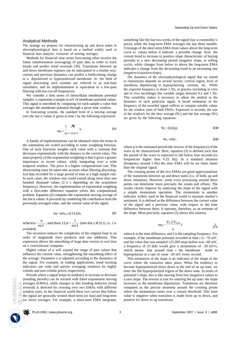
PLoS ONE | www.plosone.org 3 September 2007 | Issue 9 | e888
Separating Up and Down States
f 5
Analytical Methods The strategy we propose for characterizing up and down states in electrophysiological data is based on a method widely used in financial data analysis: crossover of moving averages.
Methods for financial time series forecasting often involve the linear transformation (averaging) of past data in order to track trends and predict trend reversals [38]. Transitions between up and down membrane regimes can be anticipated in a similar way: current and previous dynamics can predict a forthcoming change to a depolarized or hyperpolarized membrane. In the field of signal processing such systems are referred to as real-time smoothers, and its implementation is equivalent to a low-pass filtering with two cut-off frequencies.
We consider a time series of intracellular membrane potential samples. xi represents a sample in mV of membrane potential values. This signal is smoothed by computing for each sample a value that averages the membrane potential through a given time window.
In forecasting systems, the standard form of a moving average over the last n values is given at time t by the following expression:
something like the last two weeks of the signal (say a commodity’s price), while the long-term EMA averages the last three months. Crossings of the short-term EMA from values above the long-term curve to values below it indicate a possible change from the current trend to increase (a positive slope characteristic of buying periods) to a new decreasing period (negative slope, or selling cycle), while changes from below to above the long-term EMA indicates a change from the decreasing trend to an increasing one (negative to positive slope).
The dynamics of the electrophysiological signal that we intend to characterize depends on several factors: cortical region, level of anesthesia, depolarizing or hyperpolarizing currents, etc. While the expected frequency is about 1 Hz, in practice (including in vitro and in vivo recordings) this variable ranges between 0.2 and 1 Hz. This variability makes it necessary to adjust the method to the dynamics of each particular signal. A broad estimation of the frequency of the recorded signal suffices to compute suitable values for the window sizes of both EMAs. Expressed in seconds, the size of the windows for the slow average (Ws) and the fast average (Wf) are given by the following equations:
1
mt~ n
t X i~t{nz1
xi ð1Þ
Ws~2(4{p) ð3Þ
A family of implementations can be obtained when the terms in
the summation are scaled according to some weighting function. One of such functions weights each value with a constant that decreases exponentially with the distance to the current value. The main property of this exponential weighting is that it gives a greater importance to recent values, while integrating over a wide temporal window. The price is a higher computational cost. This shortcoming must be taken into account when filtering physiolog- ical data recorded for a large period of time at a high sample rate. In such cases, the window size could extend along more than one hundred thousand values (2–3 s depending on the acquisition frequency). However, the implementation of exponential weighting with a first-order difference equation solves this computational problem. Equation (2) computes the exponential moving average of the last n values. It proceeds by combining the contribution from the previously averaged value, and the current value of the signal.
mt~amt{1z(1{a)xt ð2Þ
Wf ~6Ws ð4Þ
where p is the estimated period (the inverse of the frequency) of the wave to be characterized. Here, equation (3) is defined such that the period of the wave is expected to fall below four seconds (or frequencies higher than 0.25 Hz). In a standard situation (frequency around 1 Hz) the slow EMA will be six times faster than the original signal.
The crossing points of the two EMAs are good approximations of the transitions between up and down states (i.e. of both, up and down initiation). However, some extra processing around these points can determine more precisely the onsets and offsets. The results clearly improve by analyzing the slope of the signal with a simple momentum operation. The momentum is another indicator widely used in the financial world to measure market’s sentiment. It is defined as the difference between the current value of the signal and a previous value, with respect to the time difference between them. It operates, therefore, as an estimate of the slope. More precisely, equation (5) shows this relation.
wherea~
excluded).
n
nz1
, and then 1{a~
1
nz1
(note that a M [0,1), i.e. 1 is
mt~
Vt {Vt{k
k ð Þ
The recursion reduces the complexity of the original loop to an order of magnitude (two products and one addition). This expression allows the smoothing of large data vectors in real time on a conventional computer.
Higher values of n will expand the range of past values that influence the current value, strengthening the smoothing effect of the average. Parameter n is adjusted according to the dynamics of the signal. For example, in trading applications, trend tracking indicators use wide and narrow averaging windows for highly volatile and non-volatile prices, respectively.
Periods where a signal keeps its tendency to increase or decrease (trending periods) can be tracked with fitted exponential moving averages (EMAs), while changes in this trending behavior (trend reversal) is detected by crossing over two EMAs with different window sizes. In the financial world these two curves that follow the signal are generally termed short-term (or fast) and long-term (or slow) averages. For example, a short-term EMA integrates
where k is the time difference, and f is the sampling frequency. For example, if the membrane potential recorded at time t is –70 mV, and the value that was sampled 125,000 steps before was –60 mV, a frequency of 25 kHz would give a momentum of –20 mV/s, which means that around time t the membrane tends to hyperpolarize at a rate of some –20 mV every second.
This estimation of the slope is an indicator of the shape of the curve where the transition takes place. When the tendency to become hyperpolarized slows down at the end of an up state, we enter the flat hyperpolarized region of the down state. In terms of potential’s slope, this is like moving from low (negative) values to a zero slope. The reverse is true for entering the up state: the slope increases as the membrane depolarizes. Transitions are therefore computed as the precise moments around the crossing points where the momentum raises over a certain threshold. This limit value is negative when transition is made from up to down, and positive for down to up transitions.
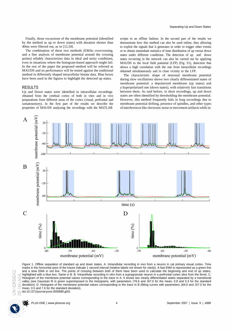
PLoS ONE | www.plosone.org 4 September 2007 | Issue 9 | e888
Separating Up and Down States
Finally, those excursions of the membrane potential (identified by the method as up or down states) with duration shorter than 40ms were filtered out, as in [12,34].
The combination of these two methods (EMAs overcrossing, and a fine analysis of membrane potential around the crossing points) reliably characterizes data in ideal and noisy conditions, even in situations where the histogram-based approach might fail. In the rest of the paper the proposed method will be referred as MAUDS and its performance will be tested against the traditional method in differently shaped intracellular bistate data. Blue boxes have been used in the figures to highlight the detected up states. RESULTS Up and Down states were identified in intracellular recordings obtained from the cerebral cortex of both in vitro and in vivo preparations from different areas of the cortex (visual, prefrontal and somatosensory). In the first part of the results we describe the properties of MAUDS analyzing the recordings with the MATLAB
scripts in an offline fashion. In the second part of the results we demonstrate how this method can also be used online, thus allowing to exploit the signals that it generates in order to trigger other events or to obtain immediate statistics of time distribution of up versus down states under different conditions. The detection of up and down states occurring in the network can also be carried out by applying MAUDS to the local field potential (LFP) (Fig. S1), detection that shows a high correlation with the one from intracellular recordings obtained simultaneously and in close vicinity to the LFP.
The characteristic shape of neuronal membrane potential during slow oscillations shows two clearly differentiated states of membrane potential: a depolarized membrane (up states) and a hyperpolarized one (down states), with relatively fast transitions between them. As said before, in short recordings, up and down states are often identified by thresholding the membrane potential. However, this method frequently fails in long recordings due to membrane potential drifting, presence of spindles, and other types of interferences like electronic noise or movement artifacts while in
Figure 1. Offline separation of standard up and down states. A. Intracellular recording in vivo from a neuron in cat primary visual cortex. Time marks in the horizontal axes of the traces indicate 1 second interval (relative labels not shown for clarity). A fast EMA is represented as a green line and a slow EMA in red line. The points of crossing between both of them have been used to calculate the beginning and end of up states, highlighted with a blue box. Same in B. B. Intracellular recording in vitro from a supragranular neuron in a prefrontal cortex slice from the ferret. C. Histogram of the membrane potential values corresponding to the trace in A. It shows two clearly differentiated states separated by a transitional valley (see Gaussian fit in green superimposed to the histograms, with parameters 276.6 and 267.0 for the mean, 0.8 and 5.3 for the standard deviation). D. Histogram of the membrane potential values corresponding to the trace in B (fitting curves with parameters 264.6 and 257.0 for the mean, 0.5 and 7.6 for the standard deviation). doi:10.1371/journal.pone.0000888.g001

PLoS ONE | www.plosone.org 5 September 2007 | Issue 9 | e888
Separating Up and Down States
vivo (heartbeat pulsation, respiratory movements, etc). Even when the aim of the experimentalists should be to eliminate all these artifacts, we will exploit them here in order to test the robustness of the described method against other commonly used ones. Two problems have to be solved for a good characterization of the states: (1) determining the periods where depolarized (up) or hyperpolarized (down) membrane potential take place, and (2) identifying the precise points in time where these states actually start and end. As explained in the previous section, MAUDS tackles these problems with an initial broad identification of the
down states by overcrossing two moving averages, and a later refinement of the initiation and termination points by a discrete processing of the membrane potential evolution in the transition interval. In general, we have observed that MAUDS performs well for any value of the long-term EMA in a wide range. On the other hand, the characterization is slightly more sensitive to the fast EMA. An optimum window size would smooth efficiently the high frequency changes of the membrane potential (isolated spikes and artifacts), being also quick enough to detect fast excursions of the signal to highly hyperpolarized regions.
Figure 2. Offline up and down states separation in drifted recordings. A. In vivo intracellular recording from a neuron in the primary visual cortex from the cat. A drift in the membrane potential is illustrated. B. Intracellular recording in vitro from a neuron in the prefrontal cortex of the ferret. The slow EMA follows the average membrane potential, providing a value of reference that discriminates the up and down levels. See the high frequencies detailed in the inset. Time marks in the horizontal axes of the traces indicate 1 second interval. C and D. Histograms corresponding the A and B traces respectively. Note that in the drifted recordings the bimodality of the Vm values is not as clear as in stable recordings like in Fig. 1. doi:10.1371/journal.pone.0000888.g002

PLoS ONE | www.plosone.org 6 September 2007 | Issue 9 | e888
Separating Up and Down States
We studied periods of $ 900 seconds of intracellular fluctuations in recordings from neurons in the visual cortex of the anesthetized cat, from neurons in the somatosensorial cortex in the anesthetized rat, and from neurons recorded in oscillating ferret cortical slices obtained from prefrontal or visual cortices from the ferret (n = 20). The traces in (Fig. 1A, 1B) were recorded from two different animals and show the standard up-down behavior. These states are efficiently separated for a wide range of fast and slow EMAs. Under these recording conditions, the histograms show two different distributions
of membrane potentials (Fig. 1C and D). Therefore, a simple thresholding is expected to reliably separate up and down states. (Overshadowing blue boxes show the precise limits of the up states found by MAUDS, in this and the following figures.)
Non-standard up and down states arise when the recording scenario departs from these ideal conditions. The periodicity and homogeneity of the standard up and down states disappears, yielding either irregular fluctuations (induced for example by noise or respiration if in vivo), or high frequencies that blur the transitions
Figure 3. Offline detection of up and down states by MAUDS in special situations. A and B. Correctly identifying up states where no action potentials occur in highly hyperpolarized neurons recorded in vitro in prefrontal cortex from the ferret. Note that in B there is correct detection of down states in spite of the repetitive occurrence of short lasting sharp events. C. Filtering isolated synaptic events occurring in the middle of a down state. D. Sorting suspicious down states intermingled into long-lasting up states (third up state). C and D correspond to intracellular recordings obtained in vivo from cat’s primary visual cortex. In all panels time marks in the horizontal axes of the traces indicate 1 second interval. doi:10.1371/journal.pone.0000888.g003
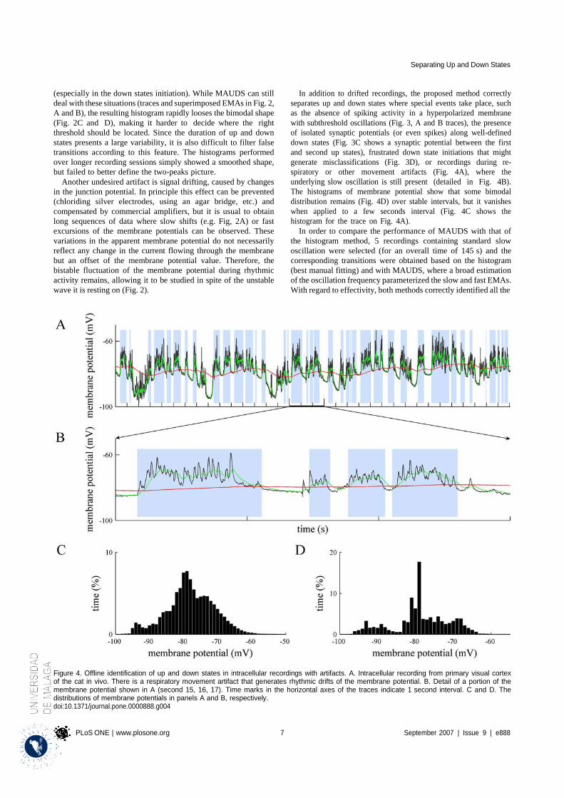
PLoS ONE | www.plosone.org 7 September 2007 | Issue 9 | e888
Separating Up and Down States
(especially in the down states initiation). While MAUDS can still deal with these situations (traces and superimposed EMAs in Fig. 2, A and B), the resulting histogram rapidly looses the bimodal shape (Fig. 2C and D), making it harder to decide where the right threshold should be located. Since the duration of up and down states presents a large variability, it is also difficult to filter false transitions according to this feature. The histograms performed over longer recording sessions simply showed a smoothed shape, but failed to better define the two-peaks picture.
Another undesired artifact is signal drifting, caused by changes in the junction potential. In principle this effect can be prevented (chloriding silver electrodes, using an agar bridge, etc.) and compensated by commercial amplifiers, but it is usual to obtain long sequences of data where slow shifts (e.g. Fig, 2A) or fast excursions of the membrane potentials can be observed. These variations in the apparent membrane potential do not necessarily reflect any change in the current flowing through the membrane but an offset of the membrane potential value. Therefore, the bistable fluctuation of the membrane potential during rhythmic activity remains, allowing it to be studied in spite of the unstable wave it is resting on (Fig. 2).
In addition to drifted recordings, the proposed method correctly separates up and down states where special events take place, such as the absence of spiking activity in a hyperpolarized membrane with subthreshold oscillations (Fig. 3, A and B traces), the presence of isolated synaptic potentials (or even spikes) along well-defined down states (Fig. 3C shows a synaptic potential between the first and second up states), frustrated down state initiations that might generate misclassifications (Fig. 3D), or recordings during re- spiratory or other movement artifacts (Fig. 4A), where the underlying slow oscillation is still present (detailed in Fig. 4B). The histograms of membrane potential show that some bimodal distribution remains (Fig. 4D) over stable intervals, but it vanishes when applied to a few seconds interval (Fig. 4C shows the histogram for the trace on Fig. 4A).
In order to compare the performance of MAUDS with that of the histogram method, 5 recordings containing standard slow oscillation were selected (for an overall time of 145 s) and the corresponding transitions were obtained based on the histogram (best manual fitting) and with MAUDS, where a broad estimation of the oscillation frequency parameterized the slow and fast EMAs. With regard to effectivity, both methods correctly identified all the
Figure 4. Offline identification of up and down states in intracellular recordings with artifacts. A. Intracellular recording from primary visual cortex of the cat in vivo. There is a respiratory movement artifact that generates rhythmic drifts of the membrane potential. B. Detail of a portion of the membrane potential shown in A (second 15, 16, 17). Time marks in the horizontal axes of the traces indicate 1 second interval. C and D. The distributions of membrane potentials in panels A and B, respectively. doi:10.1371/journal.pone.0000888.g004
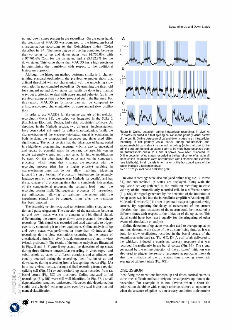
PLoS ONE | www.plosone.org 8 September 2007 | Issue 9 | e888
Separating Up and Down States
up and down states present in the recordings. On the other hand, the precision of MAUDS was compared to the histogram-based characterization according to the Coincidence Index (CoIn) described in [34]. The mean degree of overlap computed between the two series of up and down states was 91.760.8%, with a 97.761.6% CoIn for the up states, and a 85.762.8% for the down states. This value shows that MAUDS has a high precision in determining the transitions with respect to the traditional histogram approach.
Although the histogram method performs similarly in charac- terizing standard oscillations, the previous examples show that a fixed threshold will not characterize well the underlying slow oscillation in non-standard recordings. Determining the threshold for standard up and down states can easily be done in a manual way, but a criterion to deal with non-standard behavior (as in the previous examples) has not been proposed yet in the literature. For this reason, MAUDS performance can not be compared to a histogram-based characterization of non-standard slow oscilla- tions.
In order to use MAUDS for the online analysis of intracellular recordings (Movie S1), the script was integrated in the Spike 2 (Cambridge Electronic Design, Ltd.) data acquisition software. As described in the Methods section, two different implementations have been coded and tested for online characterization. While the characterization of the electrophysiological signal is equivalent in both versions, the computational resources and times used differ significantly. The script version has the advantage of being coded in a high-level programming language, which is easy to understand and update by potential users. In contrast, the assembly version results extremely cryptic and is not suited for further modification by users. On the other hand, the script runs on the computer’s processor, which means that it shares the resources with the recording process (that has a higher priority) resulting in characterization times that do not allow real-time triggering (around 1 s on a Pentium IV processor). Furthermore, the assembly language runs on the sequencer (see Methods for details), and has the advantage of a processing time that is completely independent of the computational resources, the system’s load, and the recording process itself. The sequencer processes 20 instructions per millisecond, allowing a real-time interaction with the experiment: stimuli can be triggered 1 ms after the transition has been detected.
The assembly version was used to perform online characteriza- tion and pulse triggering. The detection of the transitions between up and down states was set to generate a 1-bit digital signal, differentiating the current up or down state present in the voltage recordings. This signal was recorded and used externally to trigger events by connecting it to other equipment. Online analysis of up and down states was performed in more than 40 intracellular recordings during slow oscillations occurring in the cortex of anesthetized animals in vivo (visual, somatosensory) and in vitro (visual, prefrontal). The results of the online analysis are illustrated in Figs. 5 and 6. Figure 5 represents the detection of up states during three different intracellular recording in vivo: supra- and subthreshold up states of different durations and amplitudes are equally detected during the recording. Identification of up and down states during recording from a fast spiking neuron (Fig. 5A) in primary visual cortex, during a drifted recording from a regular spiking cell (Fig. 5B) or subthreshold up states recorded from rat barrel cortex (Fig. 5C) are illustrated. Online analyzed drifted recordings (Fig. 5B) were still well identified. In Fig. 5B a small depolarization remained undetected. However this depolarization could hardly be defined as up states even by visual inspection and manual classification.
Figure 5. Online detection during intracellular recordings in vivo. A. Up states recorded in a fast spiking neuron in the primary visual cortex of the cat. B. Online detection of up and down states in an intracellular recording in cat primary visual cortex during subthreshold and suprathreshold up states in a drifted recording (note that due to the drift the suprathreshold up states seem to be more hyperpolarized than the subthreshold ones). In A and B spikes have been truncated. C. Online detection of up states recorded in the barrel cortex of a rat. In all these cases the animals were anesthetized with ketamine and xylazine (see Methods). In all panels time marks in the horizontal axes of the traces indicate 1 second interval. doi:10.1371/journal.pone.0000888.g005
In vitro recordings were also analyzed online (Fig. 6A,B; Movie
S1), and subthreshold up states are displayed, along with the population activity reflected in the multiunit recording in close vicinity of the intracellularly recorded cell. In a different neuron (Fig. 6B), the signal generated by the detection of the initiation of the up states was fed into the intracellular amplifier (Axoclamp 2B, Molecular Devices Co.) in order to generate a step of hyperpolarizing current. By regulating the delay of occurrence of the current injection, the input resistance of the neuron could be measured at different times with respect to the initiation of the up states. This signal could have been used equally for the triggering of other events of stimulation or analysis.
Online detection of up states was also used to average up states and thus determine the shape of the up state rising time, as it was done for slow oscillations recorded in the barrel cortex of the ketamine-anesthetized rat (Fig. 6 C, D). A puff of air delivered to the whiskers induced a consistent sensory response that was recorded intracellularly in the barrel cortex (Fig. 6F). The signal generated by the online detection of the up states’ initiation was also used to trigger the sensory responses at particular intervals after the initiation of the up states, thus allowing systematic average of different trials (Fig. 6G). DISCUSSION Identifying the transitions between up and down cortical states is sometimes difficult and has to rely on the subjective opinion of the researcher. For example, it is not obvious when a short de- polarization should be wide enough to be considered an up state or when the absence of spikes is a necessary condition to determine
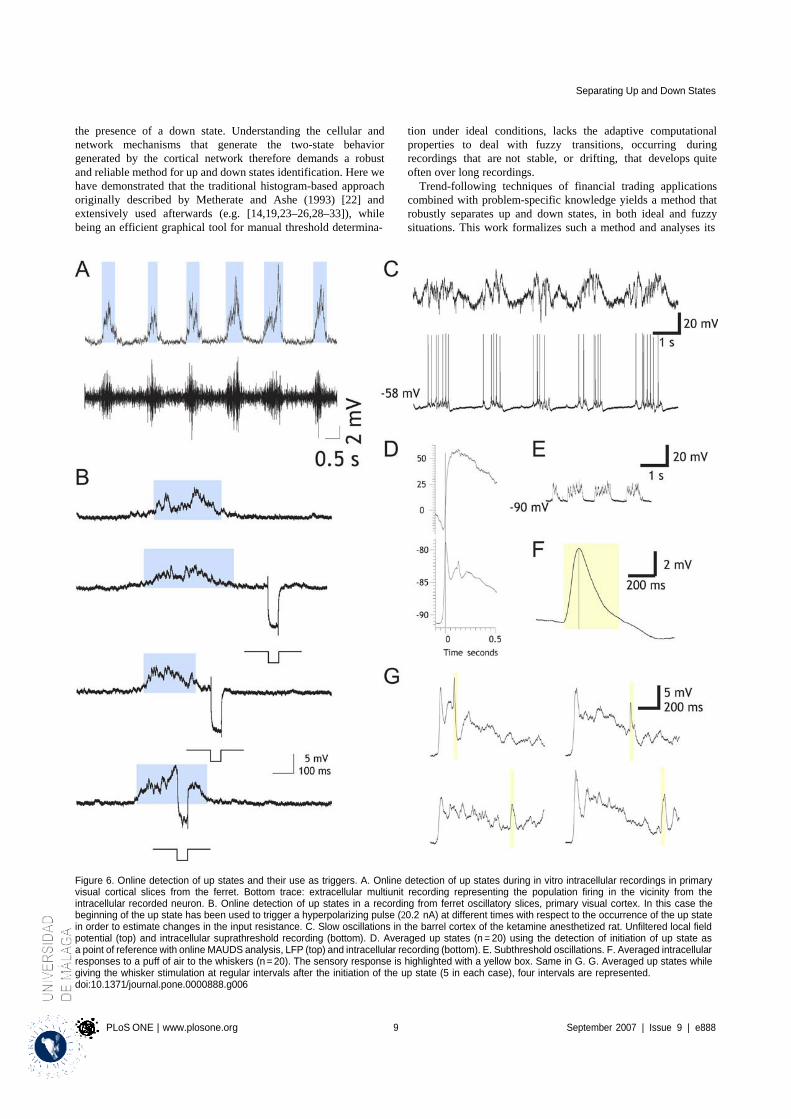
PLoS ONE | www.plosone.org 9 September 2007 | Issue 9 | e888
Separating Up and Down States
the presence of a down state. Understanding the cellular and network mechanisms that generate the two-state behavior generated by the cortical network therefore demands a robust and reliable method for up and down states identification. Here we have demonstrated that the traditional histogram-based approach originally described by Metherate and Ashe (1993) [22] and extensively used afterwards (e.g. [14,19,23–26,28–33]), while being an efficient graphical tool for manual threshold determina-
tion under ideal conditions, lacks the adaptive computational properties to deal with fuzzy transitions, occurring during recordings that are not stable, or drifting, that develops quite often over long recordings.
Trend-following techniques of financial trading applications combined with problem-specific knowledge yields a method that robustly separates up and down states, in both ideal and fuzzy situations. This work formalizes such a method and analyses its
Figure 6. Online detection of up states and their use as triggers. A. Online detection of up states during in vitro intracellular recordings in primary visual cortical slices from the ferret. Bottom trace: extracellular multiunit recording representing the population firing in the vicinity from the intracellular recorded neuron. B. Online detection of up states in a recording from ferret oscillatory slices, primary visual cortex. In this case the beginning of the up state has been used to trigger a hyperpolarizing pulse (20.2 nA) at different times with respect to the occurrence of the up state in order to estimate changes in the input resistance. C. Slow oscillations in the barrel cortex of the ketamine anesthetized rat. Unfiltered local field potential (top) and intracellular suprathreshold recording (bottom). D. Averaged up states (n = 20) using the detection of initiation of up state as a point of reference with online MAUDS analysis, LFP (top) and intracellular recording (bottom). E. Subthreshold oscillations. F. Averaged intracellular responses to a puff of air to the whiskers (n = 20). The sensory response is highlighted with a yellow box. Same in G. G. Averaged up states while giving the whisker stimulation at regular intervals after the initiation of the up state (5 in each case), four intervals are represented. doi:10.1371/journal.pone.0000888.g006

Separating Up and Down States
PLoS ONE | www.plosone.org 10 September 2007 | Issue 9 | e888
performance in different situations characteristic of ill-defined biphasic behavior: (1) irregular shape of up and down states – variations in amplitude, frequency– (Fig. 3) (2) imprecise down state initiation, (3) signal drifting (caused by changes in the liquid junction potential at the electrode tip), or (4) artifacts due to movements during in vivo recordings, such as respiratory move- ments or heartbeat (Fig. 2).
The experiments carried out for up and down state separation show that histogram-based methods will perform well in ideal situations (as widely reported in the literature), but will fail if the signal differs from this harmonic, well-defined and non-trended behavior. On the other hand, MAUDS efficiently separates up and down states in ideal (closely fitting the best histogram-based characterization) as well as in irregular oscillation. The cases studied in this work are common in most intracellular recordings, and can be analyzed with an adaptive method of the sort of MAUDS.
Well-defined up and down states have been widely studied in the past, but how this bistate behavior departs from ideal conditions has not been reported in the literature, perhaps because of the lack of objective methods to characterize irregular situations. Such a method will allow formal quantification of these excursions, and must be based on an extended definition of the up and down states that meets conflicting experimenters’ criteria. The authors believe that an algorithmic approach similar to the one presented here would definitely be a good starting point in this direction.
In order to integrate the online and offline versions, the model has been defined and tested with EMAs that compute only previous values. This is at the cost of a delay in the turning points obtained, which affects the overall performance. An offline version based on EMAs that average past and future intervals of time for each value would improve the results shown here. In spite of this delay, the predictive character of the online version has been used experimentally to trigger stimuli and to manipulate cell membrane voltage at specific times along the oscillation. This is of great interest for experimentalists to study the impact of up and down states on signal processing (e.g. changes in conductance or in synaptic transmission and plasticity). Exponential weighting has proved to perform well, since it reacts faster, minimizing the lag between the predictive moving average and the actual data. The method is also expected to perform well in this type of interactive experiments, since the presence of sensory stimuli, current injection, or other manipulations interspersed with the oscillation will not interfere with the turning points. Only the presence of short down states might be problematic, since the artifacts might cut them. The general approach exposed here would be easily fitted to the conditions of particular experimental settings.
The method formalized in this paper has been coded as a Spike 2 script, an assembly program, and also embedded in a MATLAB toolbox. All these programs are available online as an open-source code. The MATLAB implementation exploits fast matrix opera- tions and the powerful graphical capabilities of this programming language, and can analyze electrophysiological raw data formatted as ASCII or MATLAB binary files. The code has been optimized
and computes more than a million membrane potential samples per second on a PIV 2.8GHz with 0.5GB memory (this computer processes a file containing 10 minutes of intracellular membrane potential sampled at 25 kHz in some 13 seconds). On the other hand, the Spike 2 implementations are designed for online data processing, allowing real-time characterization and visualization (script version), and triggering of stimuli (sequencer version).
Further work has to be done in order to improve two different aspects of MAUDS: (1) the adaptive capabilities of the proposed method, by automatically setting the window size of the fast EMA, that can be done based on local membrane potential variability, or exploring ranges of values where the separation remains stable; and (2) a complete validation of MAUDS over an extensive set of intracellular and extracellular data (Fig. S1) recorded in different cortical areas. While the authors expect a good general performance, even with minor changes in the parameter set, the forum set up in the MAUDS website is expected to feedback about this question, as more experimenters report on the application of MAUDS to recorded datasets. SUPPORTING INFORMATION Figure S1 MAUDS detection of up and down states on the Local Field Potential recording and comparison with detection in the intracellular recording. Intracellular (A) and LFP (B) simultaneous recording in the rat barrel cortex. LFP was recorded unfiltered. MAUDS analysis has been applied off-line to both channels independently. Blue boxes highlight the detected up states in each of the recordings. Applying the concept of Coincidence Index (CoIn) described in (Mukovski et al. Cerebral Cortex 17:400, 2007), computed CoIn between both channels was 85.7%, with a 89.3% CoIn for the up states and a 82.1% for the down states. Found at: doi:10.1371/journal.pone.0000888.s001 (0.55 MB TIF)
Movie S1 Online detection of up and down states applying MAUDS to the intracellular recordings. Slow rhythm recorded in the barrel cortex of an anesthetized rat. Top panel: Online up states detection (trace going up), Middle panel: Unfiltered LFP. Bottom panel: Intracellular recording. Found at: doi:10.1371/journal.pone.0000888.s002 (2.23 MB SWF) ACKNOWLEDGMENTS We thank R. Reig and M. Winograd for their participation in the experiments, and J.-M. Alonso and L.-M. Martınez for their critical comments on a preliminary version of the manuscript.
Author Contributions Conceived and designed the experiments: MS YS FV. Performed the experiments: MS DL YS FV. Analyzed the data: MS DL YS FV. Contributed reagents/materials/analysis tools: MS DL YS FV JN. Wrote the paper: MS DL YS FV.
REFERENCES
1. Steriade M, Nunez A, Amzica F (1993) A novel slow (,1 Hz) oscillation of neocortical neurons in vivo: depolarizing and hyperpolarizing components. J Neurosci 13: 3252–3265.
2. Steriade M, Amzica F, Contreras D (1996) Synchronization of fast (30–40 Hz) spontaneous cortical rhythms during brain activation. J Neurosci 16: 392–417.
3. Cowan RL, Wilson CJ (1994) Spontaneous firing patterns and axonal projections of single corticostriatal neurons in the rat medial agranular cortex. J Neurophysiol 71: 17–32.
4. Lampl I, Reichova I, Ferster D (1999) Synchronous membrane potential fluctuations in neurons of the cat visual cortex. Neuron 22: 361–374.
5. Stern EA, Kincaid AE, Wilson CJ (1997) Spontaneous subthreshold membrane potential fluctuations and action potential variability of rat corticostriatal and striatal neurons in vivo. J Neurophysiol 77: 1697–1715.
6. Achermann P, Borbely AA (1997) Low-frequency (,1 Hz) oscillations in the human sleep electroencephalogram. Neuroscience 81: 213–222.
7. Amzica F, Steriade M (1997) The K-complex: its slow (,1-Hz) rhythmicity and relation to delta waves. Neurology 49: 952–959.
Separating Up and Down States
PLoS ONE | www.plosone.org 11 September 2007 | Issue 9 | e888
8. Simon NR, Manshanden I, Lopes da Silva FH (2000) A MEG study of sleep.
Brain Res 860: 64–76. 9. Steriade M, Nunez A, Amzica F (1993) Intracellular analysis of relations
between the slow (,1 Hz) neocortical oscillation and other sleep rhythms of the electroencephalogram. J Neurosci 13: 3266–3283.
10. Amzica F, Steriade M (1995) Short- and long-range neuronal synchronization of the slow (,1 Hz) cortical oscillation. J Neurophysiol 73: 20–38.
11. Massimini M, Huber R, Ferrarelli F, Hill S, Tononi G (2004) The sleep slow oscillation as a traveling wave. J Neurosci 24: 6862–6870.
12. Volgushev M, Chauvette S, Mukovski M, Timofeev I (2006) Precise long-range synchronization of activity and silence in neocortical neurons during slow-wave oscillations [corrected]. J Neurosci 26: 5665–5672.
13. Timofeev I, Grenier F, Bazhenov M, Sejnowski TJ, Steriade M (2000) Origin of slow cortical oscillations in deafferented cortical slabs. Cereb Cortex 10: 1185–1199.
14. Sanchez-Vives MV, McCormick DA (2000) Cellular and network mechanisms of rhythmic recurrent activity in neocortex. Nat Neurosci 3: 1027–1034.
15. Azouz R, Gray CM (1999) Cellular mechanisms contributing to response variability of cortical neurons in vivo. J Neurosci 19: 2209–2223.
16. Crochet S, Chauvette S, Boucetta S, Timofeev I (2005) Modulation of synaptic transmission in neocortex by network activities. Eur J Neurosci 21: 1030–1044.
17. Haider B, Duque A, Hasenstaub AR, McCormick DA (2006) Neocortical network activity in vivo is generated through a dynamic balance of excitation and inhibition. J Neurosci 26: 4535–4545.
18. McCormick DA, Shu Y, Hasenstaub A, Sanchez-Vives M, Badoual M, Bal T (2003) Persistent cortical activity: mechanisms of generation and effects on neuronal excitability. Cereb Cortex 13: 1219–1231.
19. Petersen C, Hahn T, Mehta M, Grinvald A, Sakmann B (2003) Interaction of sensory responses with spontaneous depolarization in layer 2/3 barrel cortex. Proc Natl Acad Sci U S A 100: 13638–13643.
20. Sachdev RN, Ebner FF, Wilson CJ (2004) Effect of subthreshold up and down states on the whisker-evoked response in somatosensory cortex. J Neurophysiol 92: 3511–3521.
21. Timofeev I, Contreras D, Steriade M (1996) Synaptic responsiveness of cortical and thalamic neurones during various phases of slow sleep oscillation in cat. Journal of Physiology-London 494: 265–278.
22. Metherate R, Ashe JH (1993) Ionic flux contributions to neocortical slow waves and nucleus basalis mediated activation - whole-cell recordings in-vivo. J Neurosci 13: 5312–5323.
23. Anderson J, Lampl I, Reichova I, Carandini M, Ferster D (2000) Stimulus dependence of two-state fluctuations of membrane potential in cat visual cortex. Nat Neurosci 3: 617–621.
24. Benucci A, Verschure PF, Konig P (2004) Two-state membrane potential fluctuations driven by weak pairwise correlations. Neural Comput 16: 2351–2378.
25. Crochet S, Fuentealba P, Timofeev I, Steriade M (2004) Selective amplification of neocortical neuronal output by fast prepotentials in vivo. Cereb Cortex 14: 1110–1121.
26. Fuentealba P, Steriade M (2005) Thalamic oscillations modulate membrane properties of cat thalamic reticular neurons. Thal Rel Syst in press.
27. Holcman D, Tsodyks M (2006) The emergence of up and down states in cortical networks. PLoS Comput Biol 2: e23.
28. Kasanetz F, Riquelme LA, Murer MG (2002) Disruption of the two-state membrane potential of striatal neurones during cortical desynchronisation in anaesthetised rats. J Physiol 543: 577–589.
29. Lewis BL, O’Donnell P (2000) Ventral tegmental area afferents to the prefrontal cortex maintain membrane potential ‘up’ states in pyramidal neurons via D(1) dopamine receptors. Cereb Cortex 10: 1168–1175.
30. Mahon S, Deniau JM, Charpier S (2003) Various synaptic activities and firing patterns in cortico-striatal and striatal neurons in vivo. J Physiol Paris 97: 557–566.
31. Peters Y, Barnhardt NE, O’Donnell P (2004) Prefrontal cortical up states are synchronized with ventral tegmental area activity. Synapse 52: 143–152.
32. Timofeev I, Grenier F, Steriade M (2001) Disfacilitation and active inhibition in the neocortex during the natural sleep-wake cycle: an intracellular study. Proc Natl Acad Sci U S A 98: 1924–1929.
33. Tseng KY, Kasanetz F, Kargieman L, Riquelme LA, Murer MG (2001) Cortical slow oscillatory activity is reflected in the membrane potential and spike trains of striatal neurons in rats with chronic nigrostriatal lesions. J Neurosci 21: 6430–6439.
34. Mukovski M, Chauvette S, Timofeev I, Volgushev M (2007) Detection of active and silent states in neocortical neurons from the field potential signal during slow-wave sleep. Cereb Cortex 17: 400–414.
35. Wilson C, Kawaguchi Y (1996) The origins of two-state spontaneous membrane potential fluctuations of neostriatal spiny neurons. J Neurosci 16: 2397–2410.
36. Aghajanian GK, Rasmussen K (1989) Intracellular studies in the facial nucleus illustrating a simple new method for obtaining viable motoneurons in adult rat brain slices. Synapse 3: 331–338.
37. Reig R, Gallego R, Nowak LG, Sanchez-Vives MV (2006) Impact of cortical network activity on short-term synaptic depression. Cereb Cortex 16: 688–695.
38. Ellinger AG (1971) The art of investment. London: Bowes and Bowes.
J Neurophysiol 106: 3035–3044, 2011. First published August 17, 2011; doi:10.1152/jn.00811.2010.
Stereotypical spatiotemporal activity patterns during slow-wave activity in the neocortex
Thomas Fucke,1 Dymphie Suchanek,1 Martin P. Nawrot,2 Yamina Seamari,3 Detlef H. Heck,4
Ad Aertsen,1,5 and Clemens Boucsein1,5
1Neurobiology and Biophysics, Faculty of Biology, and 5Bernstein Center Freiburg, University of Freiburg, Freiburg, Germany; 2Institute of Biology, Freie Universität Berlin, Berlin, Germany; 3Department of Physiology, University of Malaga, Malaga, Spain; 4Department of Anatomy and Neurobiology, University of Tennessee Health Science Center, Memphis, Tennessee
Submitted 22 September 2010; accepted in final form 11 August 2011
Fucke T, Suchanek D, Nawrot MP, Seamari Y, Heck DH, Aertsen A, Boucsein C. Stereotypical spatiotemporal activity patterns during slow-wave activity in the neocortex. J Neuro- physiol 106: 3035–3044, 2011. First published August 17, 2011; doi:10.1152/jn.00811.2010.—Alternating epochs of activity and si- lence are a characteristic feature of neocortical networks during certain sleep cycles and deep states of anesthesia. The mechanism and functional role of these slow oscillations (<1 Hz) have not yet been fully characterized. Experimental and theoretical studies show that slow-wave oscillations can be generated autonomously by neocortical tissue but become more regular through a thalamo-cortical feedback loop. Evidence for a functional role of slow-wave activity comes from EEG recordings in humans during sleep, which show that activity travels as stereotypical waves over the entire brain, thought to play a role in memory consolidation. We used an animal model to investigate activity wave propagation on a smaller scale, namely within the rat somatosensory cortex. Signals from multiple extracellular microelec- trodes in combination with one intracellular recording in the anesthe- tized animal in vivo were utilized to monitor the spreading of activity. We found that activity propagation in most animals showed a clear preferred direction, suggesting that it often originated from a similar location in the cortex. In addition, the breakdown of active states followed a similar pattern with slightly weaker direction preference but a clear correlation to the direction of activity spreading, supporting the notion of a wave-like phenomenon similar to that observed after strong sensory stimulation in sensory areas. Taken together, our findings support the idea that activity waves during slow-wave sleep do not occur spontaneously at random locations within the network, as was suggested previously, but follow preferred synaptic pathways on a small spatial scale.
slow-wave sleep; extracellular electrode array; up/down state; ket- amine/xylazine; traveling waves
SPREADING WAVES OF ACTIVITY within neocortical networks are a phenomenon that can be observed under many different con- ditions. This includes early developmental phases (Katz and Shatz 1996; Wong 1999; Momose-Sato et al. 2007), strong sensory stimulation in various primary sensory areas such as barrel cortex (Ferezou et al. 2006; Petersen et al. 2003), visual cortex (Xu et al. 2007), and motor cortices (Rubino et al. 2006) (for a detailed review see Wu et al. 2008), as well as during slow-wave sleep (Chauvette et al. 2010) and anesthesia-in- duced slow-wave activity (Steriade et al. 1993a; 1993b; 1993c;
Address for reprint requests and other correspondence: C. Boucsein, Neu-
robiology and Biophysics, Faculty of Biology, Univ. of Freiburg, Schänz- lestrasse 1, D-79104 Freiburg, Germany (e-mail: clemens.boucsein@biologie. uni-freiburg.de).
Takagaki et al. 2008). This widespread occurrence has led to a strong interest in the mechanisms underlying wave propagation in the neocortex although a functional role of the traveling waves remains unclear. To gain a better understanding of the functional nature of these reoccurring waves during slow-wave sleep, many studies have elucidated important details on the features of the so-called up- and down-states, which are a characteristic of slow-wave activity in single cells and cell populations. In a neocortical network undergoing slow-wave activity, only a certain fraction of the cells within a local volume takes part in action potential firing during the up-state (at least in the superficial layers), as was revealed by calcium imaging studies (Kerr et al. 2005), with a slow drift of the active subpopulation. Multiple parallel intracellular recordings have demonstrated, however, that even the silent cells receive nearly no synaptic input during the down-states, whereas their membrane potential shows strong depolarization and fluctua- tions during the up-states (Volgushev et al. 2006), demonstrat- ing that the entire network seems to partake in the oscillatory activity (see also Léger et al. 2005). The questions regarding which cells within the network start a new active state and the mechanisms behind its spreading are discussed somewhat con- troversially: some evidence points toward a thalamic origin (Blethyn et al. 2006; Hughes et al. 2002; Crunelli and Hughes 2010), but, because spontaneous slow-wave activity can also be observed within deafferentiated cortical slabs (Timofeev et al. 2000), it seems that the cortico-thalamic feedback loop might primarily serve to stabilize the oscillations and make them more regular (Steriade et al. 1993b; Timofeev et al. 2000). Recent in vivo studies in cats suggest that, during slow-wave sleep, layer V pyramidal neurons, generally con- sidered the output cells of the local cortical network, seem to activate before those in layer IV, which receive most of the thalamic input (Chauvette et al. 2010). Along these lines, up-state initiation in human subjects seems to be mediated by synaptic input to dendrites located in the supragranular layers, as shown by current source density analysis of layer-specific, local-field-potential recordings. However, in human cortex no leading layer in terms of onset of action potential firing could be identified (Csercsa et al. 2010). Data from acute slice experiments have supported these findings (Sanchez-Vives and McCormick 2000), and the observation that extracellular Ca2+
concentrations rapidly increase toward the end of the down- states and gradually decrease during the depolarized up-states (Massimini and Amzica 2001) has also argued in favor of the
www.jn.org
0022-3077/11 Copyright © 2011 the American Physiological Society
3035
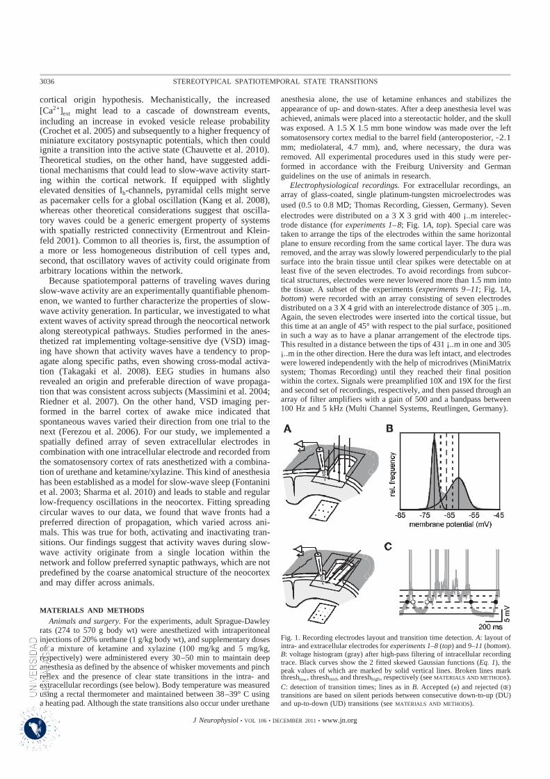
3036 STEREOTYPICAL SPATIOTEMPORAL STATE TRANSITIONS
J Neurophysiol • VOL 106 • DECEMBER 2011 • www.jn.org
cortical origin hypothesis. Mechanistically, the increased [Ca2+]ext might lead to a cascade of downstream events, including an increase in evoked vesicle release probability (Crochet et al. 2005) and subsequently to a higher frequency of miniature excitatory postsynaptic potentials, which then could ignite a transition into the active state (Chauvette et al. 2010). Theoretical studies, on the other hand, have suggested addi- tional mechanisms that could lead to slow-wave activity start- ing within the cortical network. If equipped with slightly elevated densities of Ih-channels, pyramidal cells might serve as pacemaker cells for a global oscillation (Kang et al. 2008), whereas other theoretical considerations suggest that oscilla- tory waves could be a generic emergent property of systems with spatially restricted connectivity (Ermentrout and Klein- feld 2001). Common to all theories is, first, the assumption of a more or less homogeneous distribution of cell types and, second, that oscillatory waves of activity could originate from arbitrary locations within the network.
Because spatiotemporal patterns of traveling waves during slow-wave activity are an experimentally quantifiable phenom- enon, we wanted to further characterize the properties of slow- wave activity generation. In particular, we investigated to what extent waves of activity spread through the neocortical network along stereotypical pathways. Studies performed in the anes- thetized rat implementing voltage-sensitive dye (VSD) imag- ing have shown that activity waves have a tendency to prop- agate along specific paths, even showing cross-modal activa- tion (Takagaki et al. 2008). EEG studies in humans also revealed an origin and preferable direction of wave propaga- tion that was consistent across subjects (Massimini et al. 2004; Riedner et al. 2007). On the other hand, VSD imaging per- formed in the barrel cortex of awake mice indicated that spontaneous waves varied their direction from one trial to the next (Ferezou et al. 2006). For our study, we implemented a spatially defined array of seven extracellular electrodes in combination with one intracellular electrode and recorded from the somatosensory cortex of rats anesthetized with a combina- tion of urethane and ketamine/xylazine. This kind of anesthesia has been established as a model for slow-wave sleep (Fontanini et al. 2003; Sharma et al. 2010) and leads to stable and regular low-frequency oscillations in the neocortex. Fitting spreading circular waves to our data, we found that wave fronts had a preferred direction of propagation, which varied across ani- mals. This was true for both, activating and inactivating tran- sitions. Our findings suggest that activity waves during slow- wave activity originate from a single location within the network and follow preferred synaptic pathways, which are not predefined by the coarse anatomical structure of the neocortex and may differ across animals.
MATERIALS AND METHODS
Animals and surgery. For the experiments, adult Sprague-Dawley rats (274 to 570 g body wt) were anesthetized with intraperitoneal injections of 20% urethane (1 g/kg body wt), and supplementary doses of a mixture of ketamine and xylazine (100 mg/kg and 5 mg/kg, respectively) were administered every 30 –50 min to maintain deep anesthesia as defined by the absence of whisker movements and pinch
anesthesia alone, the use of ketamine enhances and stabilizes the appearance of up- and down-states. After a deep anesthesia level was achieved, animals were placed into a stereotactic holder, and the skull was exposed. A 1.5 X 1.5 mm bone window was made over the left somatosensory cortex medial to the barrel field (anteroposterior, -2.1 mm; mediolateral, 4.7 mm), and, where necessary, the dura was removed. All experimental procedures used in this study were per- formed in accordance with the Freiburg University and German guidelines on the use of animals in research.
Electrophysiological recordings. For extracellular recordings, an array of glass-coated, single platinum-tungsten microelectrodes was used (0.5 to 0.8 MD; Thomas Recording, Giessen, Germany). Seven electrodes were distributed on a 3 X 3 grid with 400 ¡..m interelec- trode distance (for experiments 1– 8; Fig. 1A, top). Special care was taken to arrange the tips of the electrodes within the same horizontal plane to ensure recording from the same cortical layer. The dura was removed, and the array was slowly lowered perpendicularly to the pial surface into the brain tissue until clear spikes were detectable on at least five of the seven electrodes. To avoid recordings from subcor- tical structures, electrodes were never lowered more than 1.5 mm into the tissue. A subset of the experiments (experiments 9 –11; Fig. 1A, bottom) were recorded with an array consisting of seven electrodes distributed on a 3 X 4 grid with an interelectrode distance of 305 ¡..m. Again, the seven electrodes were inserted into the cortical tissue, but this time at an angle of 45° with respect to the pial surface, positioned in such a way as to have a planar arrangement of the electrode tips. This resulted in a distance between the tips of 431 ¡..m in one and 305 ¡..m in the other direction. Here the dura was left intact, and electrodes were lowered independently with the help of microdrives (MiniMatrix system; Thomas Recording) until they reached their final position within the cortex. Signals were preamplified 10X and 19X for the first and second set of recordings, respectively, and then passed through an array of filter amplifiers with a gain of 500 and a bandpass between 100 Hz and 5 kHz (Multi Channel Systems, Reutlingen, Germany).
Fig. 1. Recording electrodes layout and transition time detection. A: layout of intra- and extracellular electrodes for experiments 1–8 (top) and 9–11 (bottom). B: voltage histogram (gray) after high-pass filtering of intracellular recording trace. Black curves show the 2 fitted skewed Gaussian functions (Eq. 1), the peak values of which are marked by solid vertical lines. Broken lines mark
reflex and the presence of clear state transitions in the intra- and threshlow , threshmid , and threshhigh , respectively (see MATERIALS AND METHODS). extracellular recordings (see below). Body temperature was measured using a rectal thermometer and maintained between 38 –39° C using a heating pad. Although the state transitions also occur under urethane
C: detection of transition times; lines as in B. Accepted (e) and rejected (Œ) transitions are based on silent periods between consecutive down-to-up (DU) and up-to-down (UD) transitions (see MATERIALS AND METHODS).
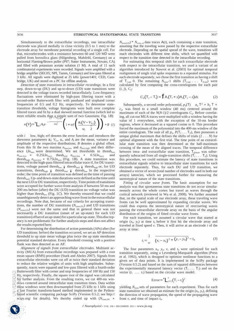
3036 STEREOTYPICAL SPATIOTEMPORAL STATE TRANSITIONS
J Neurophysiol • VOL 106 • DECEMBER 2011 • www.jn.org
2
2
7
2 +
STEREOTYPICAL SPATIOTEMPORAL STATE TRANSITIONS 3037
Simultaneously to the extracellular recordings, one intracellular electrode was placed medially in close vicinity (0.5 to 1 mm) to the electrode array for membrane potential recording of a single cell. For that, microelectrodes with a resistance between 60 and 120 MD were pulled from borosilica glass (Hilgenberg, Malsfeld, Germany) on a horizontal Flaming/Brown puller (P97; Sutter Instruments, Novato, CA) and filled with potassium acetate solution (1 M). A total of 11 such combinatorial experiments were recorded. Signals were amplified with a bridge amplifier (SEC05; NPI, Tamm, Germany) and low-pass filtered at 3 kHz. All signals were digitized at 25 kHz (power1401; CED, Cam- bridge, UK) and stored on a PC for offline analysis.
Detection of state transitions in intracellular recordings. In a first step, down-to-up (DU) and up-to-down (UD) state transitions were detected in the voltage traces recorded intracellularly. Low-frequency fluctuations were eliminated by high-pass filtering traces with a second-order Butterworth filter with passband and stopband corner
Ntrans,UD) * Nextra_el data traces A(t), each containing a state transition, assuming that the traveling wave passed by the respective extracellular electrode. Depending on the spatial spread of the wave, transitions will reach electrodes with different time shifts, which we quantified with respect to the transition time detected in the intracellular recording.
For estimating this temporal shift for each extracellular electrode with respect to the intracellular transition, we used a variant of an algorithm introduced by Nawrot et al. (2003) for optimal temporal realignment of single trial spike responses to a repeated stimulus. For each electrode separately, we chose the first transition as having a shift of T1,opt 0. The remaining Ntrans-1 shifts (T2,opt . . . TN,opt) were calculated by first computing the cross-correlograms for each pair (i, j), Cij:
Cij(T j - Ti) = f Ai(Ti + s)A j(T j - s)ds (2)
frequencies of 0.5 and 0.2 Hz, respectively. To determine state- Subsequently, a second order polynomial, pij(T) aij T + bij T + transition thresholds, voltage histograms were built over complete filtered traces and fit by a dual skewed normal function (which led to more reliable results than a simple sum of two Gaussians; Fig. 1B):
(V - V0,i)2
cij, was fitted to a small window (40 ms) centered around the maximum of each of the N(N-1)/2 correlograms Cij. Before correlat- ing, all cut-out MUA traces were multiplied with a window having the value of 1 everywhere, with the exception of the 10-ms border -
n(V) = 'Li Aie 2ui (1 + erf ( ai(V - V0,i) )) + B (1) regions, where it decreased as a squared cosine to 0. This procedure ui 2 forced the maximum of the polynomial into the 400-ms window of the
entire correlogram. The sum of all pij, P(T2 . . . TN), then possesses a with i low, high; erf denotes the error function and introduces the skewness parameters ai; V0,i, ui, and Ai are the mean, variance and amplitude of the respective distributions; B denotes a global offset. From this fit the two maxima nmax,low and nmax,high and their differ- ence Llnmax were determined. We set thresholds to threshlow nmax,low + 0.25Llnmax, theshmid nmax,low + 0.5Llnmax, and threshhigh nmax,low + 0.75Llnmax (Fig. 1B). A state transition was detected in the high-pass filtered intracellular trace if, for DU transi- tions, voltage passed threshlow ¡ threshmid ¡ threshhigh or, for UD transitions, threshhigh ¡ threshmid ¡ threshlow in the respective order; the time point of transition was defined as the time of passing threshmid. Up- and down-state durations were defined as the time until the next UD or DU transition, respectively. Time points of transitions were accepted for further wave-front analysis if between 50 ms and 200 ms before (after) the DU (UD) transition no voltage value was higher than threshlow (Fig. 1C). We thereby ensured that we could unambiguously detect an approaching wave front in the extracellular recordings. Note that, because of our criteria for accepting transi- tions, the number of DU transitions (Ntrans,DU) and UD transitions (Ntrans,UD) were not the same and that in general there was not necessarily a DU transition (onset of an up-state) for each UD transition (offset of an up-state) for a particular up-state. This discrep- ancy is not problematic for further analysis steps and does not affect the results reported here.
For determining the distribution of action potentials (APs) after (for UD transitions: before) the transition occurred, we set an AP detection
unique global maximum that defines the shifts of trials (2 . . . N) for optimal alignment with the first trial. The time point of an extracel- lular state transition was then determined as the half-maximum crossing of the mean of the aligned traces. The temporal difference between intra- and extracellular state transition, Tglobal, was subse- quently subtracted from all single-transition shifts (T1 . . . TN). Using this procedure, we could estimate the latency of state transitions in extracellular signals relative to intracellular state transitions for each electrode separately. Thus, for each DU and UD transition, we obtained a vector of seven (total number of electrodes used in both our arrays) latencies, which we processed further for measuring the stereotypical nature of the state transitions.
Fitting of circular wave fronts. The basic assumption for our analysis was that spontaneous state transitions do not occur simulta- neously across the whole cortex but travel as waves through the cortical network (reviewed in Wu et al. 2008). We further assumed that, on the spatial scale of our electrode array, these traveling wave fronts can be well approximated by expanding circular waves. We could thus express the stereotypical nature of reoccurring waves passing the extracellular electrode array on the basis of the angular distribution of the origins of fitted circular wave fronts.
For each transition, we assumed a circular wave that started at origin (x0, y0) at time t0 before it first hit the electrode array and traveled at fixed speed v. Then, it will arrive at an electrode i of the array at time:
threshold to up state mean voltage plus twice the up state membrane potential standard deviation. Every threshold crossing with a positive flank was then detected as an AP.
1
ti = v
(xi - x0) (yi - y 0)2 - t0
(3)
Alignment of signals from extracellular electrodes. Multiunit ac- tivity (MUA) from extracellular recordings was prepared with a root mean square (RMS) procedure (Stark and Abeles 2007). Signals from extracellular electrodes were cut off at twice their standard deviation to reduce the relative weights of units with high amplitudes. Subse- quently, traces were squared and low-pass filtered with a fourth-order Butterworth filter with corner and stop frequencies of 100 Hz and 150 Hz, respectively. Finally, the square root of the signal was calculated
The four parameters x0, y0, v, and t0 were optimized for each transition separately, using a Levenberg-Marquardt algorithm (Press et al. 1992), which is designed to optimize nonlinear functions to a given set of data points. It is implemented in the SciPy package (Version 0.5.2) and based on the sum of squared differences between the experimentally measured latency vector (T1 . . . T7) and on the vector (t1 . . . t7) based on the circular wave model:
for further analysis. From the resulting traces, we cut 400-ms win- dows centered around intracellular state transition times. Data within
Error = 'Li=1 (Ti - ti)2 (4)
these windows were then downsampled from 25 kHz to 1 kHz using a fast Fourier transform-based method implemented in the Python- based scientific computing package SciPy (Version 0.5.2; see http:// scipy.org/ for details). We thereby ended up with (Ntrans,DU +
yielding Ntrans sets of parameters for each experiment. Thus for each state transition we obtained an estimate for the origin (x0, y0), defining the direction of wave propagation, the speed of the propagating wave front v, and time of impact t0.
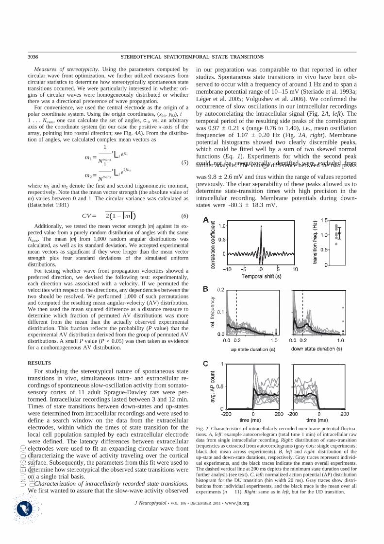
3036 STEREOTYPICAL SPATIOTEMPORAL STATE TRANSITIONS
J Neurophysiol • VOL 106 • DECEMBER 2011 • www.jn.org
3038 STEREOTYPICAL SPATIOTEMPORAL STATE TRANSITIONS
Measures of stereotypicity. Using the parameters computed by circular wave front optimization, we further utilized measures from circular statistics to determine how stereotypically spontaneous state transitions occurred. We were particularly interested in whether ori- gins of circular waves were homogeneously distributed or whether there was a directional preference of wave propagation.
For convenience, we used the central electrode as the origin of a polar coordinate system. Using the origin coordinates, (x0,i, y0,i), i 1 . . . Ntrans, one can calculate the set of angles, c.i, vs. an arbitrary axis of the coordinate system (in our case the positive x-axis of the array, pointing into rostral direction; see Fig. 4A). From the distribu- tion of angles, we calculated complex mean vectors as
1
in our preparation was comparable to that reported in other studies. Spontaneous state transitions in vivo have been ob- served to occur with a frequency of around 1 Hz and to span a membrane potential range of 10 –15 mV (Steriade et al. 1993a; Léger et al. 2005; Volgushev et al. 2006). We confirmed the occurrence of slow oscillations in our intracellular recordings by autocorrelating the intracellular signal (Fig. 2A, left). The temporal period of the resulting side peaks of the correlogram was 0.97 ± 0.21 s (range 0.76 to 1.40), i.e., mean oscillation frequencies of 1.07 ± 0.20 Hz (Fig. 2A, right). Membrane potential histograms showed two clearly discernible peaks, which could be fitted well by a sum of two skewed normal
m1 = N
trans
1
'Li e jc.i (5)
functions (Eq. 1). Experiments for which the second peak could not be unequivocally identified were excluded from
2 jc.i further analysis. The voltage difference between the two peaks
m2 = N
trans 'Li e was 9.8 ± 2.6 mV and thus within the range of values reported
where m1 and m2 denote the first and second trigonometric moment, respectively. Note that the mean vector strength (the absolute value of m) varies between 0 and 1. The circular variance was calculated as (Batschelet 1981)
CV = 2(1 - lml) (6)
Additionally, we tested the mean vector strength |m| against its ex- pected value from a purely random distribution of angles with the same Ntrans. The mean |m| from 1,000 random angular distributions was calculated, as well as its standard deviation. We accepted experimental mean vectors as significant if they were longer than the mean vector strength plus four standard deviations of the simulated uniform distributions.
For testing whether wave front propagation velocities showed a preferred direction, we devised the following test: experimentally, each direction was associated with a velocity. If we permuted the velocities with respect to the directions, any dependencies between the two should be resolved. We performed 1,000 of such permutations and computed the resulting mean angular-velocity (AV) distribution. We then used the mean squared difference as a distance measure to determine which fraction of permuted AV distributions was more different from the mean than the actually observed experimental distribution. This fraction reflects the probability (P value) that the experimental AV distribution derived from the group of permuted AV distributions. A small P value (P < 0.05) was then taken as evidence for a nonhomogeneous AV distribution.
RESULTS
For studying the stereotypical nature of spontaneous state transitions in vivo, simultaneous intra- and extracellular re- cordings of spontaneous slow-oscillation activity from somato- sensory cortex of 11 adult Sprague-Dawley rats were per- formed. Intracellular recordings lasted between 3 and 12 min. Times of state transitions between down-states and up-states were determined from intracellular recordings and were used to define a search window on the data from the extracellular electrodes, within which the times of state transition for the local cell population sampled by each extracellular electrode were defined. The latency differences between extracellular electrodes were used to fit an expanding circular wave front characterizing the wave of activity traveling over the cortical surface. Subsequently, the parameters from this fit were used to determine how stereotypical the observed state transitions were on a single trial basis.
Characterization of intracellularly recorded state transitions. We first wanted to assure that the slow-wave activity observed
previously. The clear separability of these peaks allowed us to determine state-transition times with high precision in the intracellular recording. Membrane potentials during down- states were -80.3 ± 18.3 mV.
Fig. 2. Characteristics of intracellularly recorded membrane potential fluctua- tions. A, left: example autocorrelogram (total time 1 min) of intracellular raw data from single intracellular recording. Right: distribution of state-transition frequencies as extracted from autocorrelograms (gray dots: single experiments; black dot: mean across experiments). B, left and right: distribution of the up-state and down-state durations, respectively. Gray traces represent individ- ual experiments, and the black traces indicate the mean overall experiments. The dashed vertical line at 200 ms depicts the minimum state duration used for further analysis (see text). C, left: normalized action potential (AP) distribution histogram for the DU transition (bin width 20 ms). Gray traces show distri- butions from individual experiments, and the black trace is the mean over all experiments (n 11). Right: same as in left, but for the UD transition.
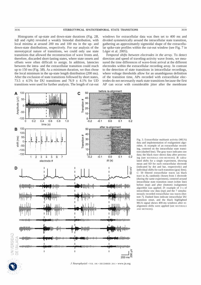
3036 STEREOTYPICAL SPATIOTEMPORAL STATE TRANSITIONS
J Neurophysiol • VOL 106 • DECEMBER 2011 • www.jn.org
STEREOTYPICAL SPATIOTEMPORAL STATE TRANSITIONS 3039
Histograms of up-state and down-state durations (Fig. 2B, left and right) revealed a weakly bimodal distribution, with local minima at around 200 ms and 100 ms in the up- and down-state distributions, respectively. For our analysis of the stereotypical nature of transitions, we could only use state transitions that allowed the reconstruction of wave fronts and, therefore, discarded short-lasting states, where state onsets and offsets were often difficult to assign. In addition, latencies between the intra- and the extracellular transition could reach up to 150 ms (Fig. 3B). As a minimum duration, we thus chose the local minimum in the up-state length distribution (200 ms). After the exclusion of state transitions followed by short states, 73.5 ± 4.5% for DU transitions and 76.9 ± 4.1% for UD transitions were used for further analysis. The length of cut-out
windows for extracellular data was then set to 400 ms and divided symmetrically around the intracellular state transition, gathering an approximately sigmoidal shape of the extracellu- lar spike-rate profiles within the cut-out window (see Fig. 7 in Léger et al. 2005).
Temporal shifts between electrodes in the array. To detect direction and speed of traveling-activity wave fronts, we mea- sured the time differences of wave-front arrival at the different electrodes within the extracellular recording array. In contrast to the detection of state transitions in intracellular recordings, where voltage thresholds allow for an unambiguous definition of the transition time, APs recorded with extracellular elec- trodes do not necessarily mark state transitions because the first AP can occur with considerable jitter after the membrane
Fig. 3. Extracellular multiunit activity (MUA) data and implementation of realignment algo- rithm. A: example of an extracellular record- ing, centered on the intracellular state transi- tion (dashed line). The gray trace indicates raw data; the black trace shows data after process- ing (see MATERIALS AND METHODS). B: calcu- lated shifts for a single experiment, showing mean and SD for each extracellular electrode (indicated by dot and bar, respectively) and individual shifts for each transition (gray dots). C: 50 filtered extracellular traces (as black trace in A), randomly chosen from 1 electrode (during the same experiment), centered around intracellular state transition onset (white line) before (top) and after (bottom) realignment algorithm was applied. D: example of 3 s of intracellular raw data (top) and the 7 simulta- neously recorded extracellular raw traces (bot- tom 7). Dashed lines indicate intracellular DU transition onset, and the black highlighted MUA signal shows 400-ms windows after re- alignment shifts were applied (see MATERIALS
AND METHODS).
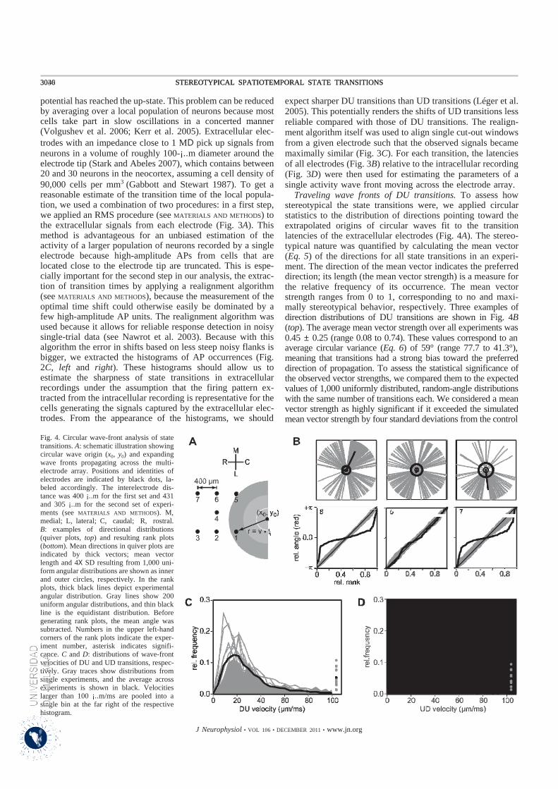
3036 STEREOTYPICAL SPATIOTEMPORAL STATE TRANSITIONS
J Neurophysiol • VOL 106 • DECEMBER 2011 • www.jn.org
3040 STEREOTYPICAL SPATIOTEMPORAL STATE TRANSITIONS
potential has reached the up-state. This problem can be reduced by averaging over a local population of neurons because most cells take part in slow oscillations in a concerted manner (Volgushev et al. 2006; Kerr et al. 2005). Extracellular elec- trodes with an impedance close to 1 MD pick up signals from neurons in a volume of roughly 100-¡..m diameter around the electrode tip (Stark and Abeles 2007), which contains between 20 and 30 neurons in the neocortex, assuming a cell density of 90,000 cells per mm3 (Gabbott and Stewart 1987). To get a reasonable estimate of the transition time of the local popula- tion, we used a combination of two procedures: in a first step, we applied an RMS procedure (see MATERIALS AND METHODS) to the extracellular signals from each electrode (Fig. 3A). This method is advantageous for an unbiased estimation of the activity of a larger population of neurons recorded by a single electrode because high-amplitude APs from cells that are located close to the electrode tip are truncated. This is espe- cially important for the second step in our analysis, the extrac- tion of transition times by applying a realignment algorithm (see MATERIALS AND METHODS), because the measurement of the optimal time shift could otherwise easily be dominated by a few high-amplitude AP units. The realignment algorithm was used because it allows for reliable response detection in noisy single-trial data (see Nawrot et al. 2003). Because with this algorithm the error in shifts based on less steep noisy flanks is bigger, we extracted the histograms of AP occurrences (Fig. 2C, left and right). These histograms should allow us to estimate the sharpness of state transitions in extracellular recordings under the assumption that the firing pattern ex- tracted from the intracellular recording is representative for the cells generating the signals captured by the extracellular elec- trodes. From the appearance of the histograms, we should
expect sharper DU transitions than UD transitions (Léger et al. 2005). This potentially renders the shifts of UD transitions less reliable compared with those of DU transitions. The realign- ment algorithm itself was used to align single cut-out windows from a given electrode such that the observed signals became maximally similar (Fig. 3C). For each transition, the latencies of all electrodes (Fig. 3B) relative to the intracellular recording (Fig. 3D) were then used for estimating the parameters of a single activity wave front moving across the electrode array.
Traveling wave fronts of DU transitions. To assess how stereotypical the state transitions were, we applied circular statistics to the distribution of directions pointing toward the extrapolated origins of circular waves fit to the transition latencies of the extracellular electrodes (Fig. 4A). The stereo- typical nature was quantified by calculating the mean vector (Eq. 5) of the directions for all state transitions in an experi- ment. The direction of the mean vector indicates the preferred direction; its length (the mean vector strength) is a measure for the relative frequency of its occurrence. The mean vector strength ranges from 0 to 1, corresponding to no and maxi- mally stereotypical behavior, respectively. Three examples of direction distributions of DU transitions are shown in Fig. 4B (top). The average mean vector strength over all experiments was 0.45 ± 0.25 (range 0.08 to 0.74). These values correspond to an average circular variance (Eq. 6) of 59° (range 77.7 to 41.3°), meaning that transitions had a strong bias toward the preferred direction of propagation. To assess the statistical significance of the observed vector strengths, we compared them to the expected values of 1,000 uniformly distributed, random-angle distributions with the same number of transitions each. We considered a mean vector strength as highly significant if it exceeded the simulated mean vector strength by four standard deviations from the control
Fig. 4. Circular wave-front analysis of state transitions. A: schematic illustration showing circular wave origin (x0, y0) and expanding wave fronts propagating across the multi- electrode array. Positions and identities of electrodes are indicated by black dots, la- beled accordingly. The interelectrode dis- tance was 400 ¡..m for the first set and 431 and 305 ¡..m for the second set of experi- ments (see MATERIALS AND METHODS). M, medial; L, lateral; C, caudal; R, rostral. B: examples of directional distributions (quiver plots, top) and resulting rank plots (bottom). Mean directions in quiver plots are indicated by thick vectors; mean vector length and 4X SD resulting from 1,000 uni- form angular distributions are shown as inner and outer circles, respectively. In the rank plots, thick black lines depict experimental angular distribution. Gray lines show 200 uniform angular distributions, and thin black line is the equidistant distribution. Before generating rank plots, the mean angle was subtracted. Numbers in the upper left-hand corners of the rank plots indicate the exper- iment number, asterisk indicates signifi- cance. C and D: distributions of wave-front velocities of DU and UD transitions, respec- tively. Gray traces show distributions from single experiments, and the average across experiments is shown in black. Velocities larger than 100 ¡..m/ms are pooled into a single bin at the far right of the respective histogram.
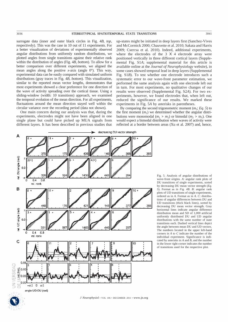
3036 STEREOTYPICAL SPATIOTEMPORAL STATE TRANSITIONS
J Neurophysiol • VOL 106 • DECEMBER 2011 • www.jn.org
STEREOTYPICAL SPATIOTEMPORAL STATE TRANSITIONS 3041
surrogate data (inner and outer black circles in Fig. 4B, top, respectively). This was the case in 10 out of 11 experiments. For a better visualization of deviations of experimentally observed angular distributions from uniformly random distributions, we plotted angles from single transitions against their relative rank within the distribution of angles (Fig. 4B, bottom). To allow for a better comparison over different experiments, we aligned the mean angles along the positive x-axis (angle 0°). This way, experimental data can be easily compared with simulated uniform distributions (gray traces in Fig. 4B, bottom). This visualization, similar to the reported mean vector lengths, demonstrates that most experiments showed a clear preference for one direction of the wave of activity spreading over the cortical tissue. Using a sliding-window (width: 10 transitions) approach, we examined the temporal evolution of the mean direction. For all experiments, fluctuations around the mean direction stayed well within the circular variance over the recording period (data not shown).
One main concern during our analysis was that, during the experiments, electrodes might not have been aligned in one single plane but could have picked up MUA signals from different layers. It has been described in previous studies that
up-states might be initiated in deep layers first (Sanchez-Vives and McCormick 2000; Chauvette et al. 2010; Sakata and Harris 2009; Csercsa et al. 2010). Indeed, additional experiments, where the electrodes of the 3 X 4 electrode array were positioned vertically in three different cortical layers (Supple- mental Fig. S1A; supplemental material for this article is available online at the Journal of Neurophysiology website), in some cases showed temporal lead in deep layers (Supplemental Fig. S1B). To test whether one electrode introduces such a systematic error to our wave-front parameter estimation, we performed the same analysis again with one electrode left out in turn. For most experiments, no qualitative changes of our results were observed (Supplemental Fig. S2A). For two ex- periments, however, we found electrodes that, when left out, reduced the significance of our results. We marked these experiments in Fig. 5A by asterisks in parentheses.
By comparing the second trigonometric moment (m2; Eq. 5) to the first moment (m1) we determined whether the angular distri- butions were monomodal (m1 > m2) or bimodal (m2 > m1). One would expect a bimodal distribution when waves of activity were reflected at a border between areas (Xu et al. 2007) and, hence,
Fig. 5. Analysis of angular distributions of wave-front origins. A: angular rank plots of DU transitions of single experiments, sorted by decreasing DU mean vector strength (Eq. 5). Format as in Fig. 4B. B: angular rank plots of UD transitions of single experiments, ordered as in A. Format as in A. C: distribu- tions of angular differences between DU and UD transitions (thick black lines), sorted by decreasing DU mean vector strength. Gray horizontal lines indicate angular difference distribution mean and SD of 1,000 artificial uniformly distributed DU and UD angular distributions with the same number of state transitions each. Dashed vertical lines depict the angle between mean DU and UD vectors. The numbers located in the upper left-hand corners in A to C indicate the number of the individual experiment. Significance is indi- cated by asterisks in A and B, and the number in the lower right corner indicates the number of transitions used for the respective plot.
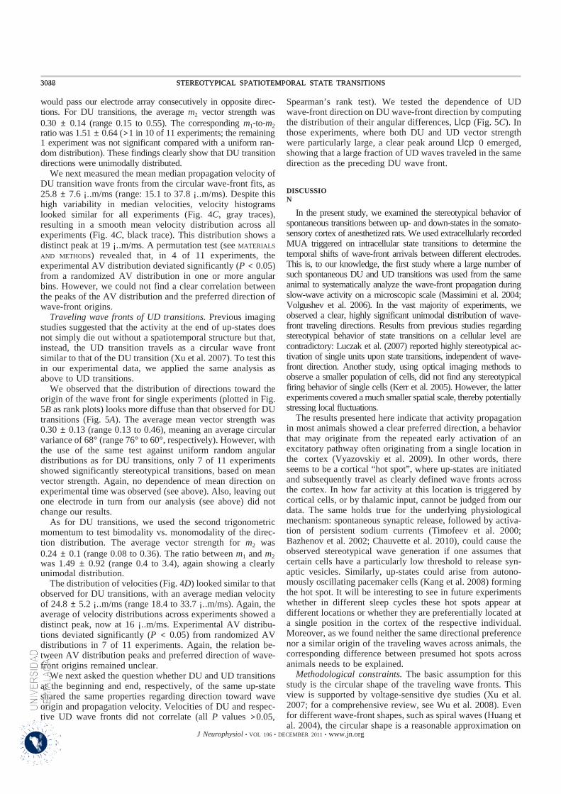
3036 STEREOTYPICAL SPATIOTEMPORAL STATE TRANSITIONS
J Neurophysiol • VOL 106 • DECEMBER 2011 • www.jn.org
3042 STEREOTYPICAL SPATIOTEMPORAL STATE TRANSITIONS
would pass our electrode array consecutively in opposite direc- tions. For DU transitions, the average m2 vector strength was 0.30 ± 0.14 (range 0.15 to 0.55). The corresponding m1-to-m2
ratio was 1.51 ± 0.64 (>1 in 10 of 11 experiments; the remaining 1 experiment was not significant compared with a uniform ran- dom distribution). These findings clearly show that DU transition directions were unimodally distributed.
We next measured the mean median propagation velocity of DU transition wave fronts from the circular wave-front fits, as 25.8 ± 7.6 ¡..m/ms (range: 15.1 to 37.8 ¡..m/ms). Despite this high variability in median velocities, velocity histograms looked similar for all experiments (Fig. 4C, gray traces), resulting in a smooth mean velocity distribution across all experiments (Fig. 4C, black trace). This distribution shows a distinct peak at 19 ¡..m/ms. A permutation test (see MATERIALS
AND METHODS) revealed that, in 4 of 11 experiments, the experimental AV distribution deviated significantly (P < 0.05) from a randomized AV distribution in one or more angular bins. However, we could not find a clear correlation between the peaks of the AV distribution and the preferred direction of wave-front origins.
Traveling wave fronts of UD transitions. Previous imaging studies suggested that the activity at the end of up-states does not simply die out without a spatiotemporal structure but that, instead, the UD transition travels as a circular wave front similar to that of the DU transition (Xu et al. 2007). To test this in our experimental data, we applied the same analysis as above to UD transitions.
We observed that the distribution of directions toward the origin of the wave front for single experiments (plotted in Fig. 5B as rank plots) looks more diffuse than that observed for DU transitions (Fig. 5A). The average mean vector strength was 0.30 ± 0.13 (range 0.13 to 0.46), meaning an average circular variance of 68° (range 76° to 60°, respectively). However, with the use of the same test against uniform random angular distributions as for DU transitions, only 7 of 11 experiments showed significantly stereotypical transitions, based on mean vector strength. Again, no dependence of mean direction on experimental time was observed (see above). Also, leaving out one electrode in turn from our analysis (see above) did not change our results.
As for DU transitions, we used the second trigonometric momentum to test bimodality vs. monomodality of the direc- tion distribution. The average vector strength for m2 was 0.24 ± 0.1 (range 0.08 to 0.36). The ratio between m1 and m2
was 1.49 ± 0.92 (range 0.4 to 3.4), again showing a clearly unimodal distribution.
The distribution of velocities (Fig. 4D) looked similar to that observed for DU transitions, with an average median velocity of 24.8 ± 5.2 ¡..m/ms (range 18.4 to 33.7 ¡..m/ms). Again, the average of velocity distributions across experiments showed a distinct peak, now at 16 ¡..m/ms. Experimental AV distribu- tions deviated significantly (P < 0.05) from randomized AV distributions in 7 of 11 experiments. Again, the relation be- tween AV distribution peaks and preferred direction of wave- front origins remained unclear.
We next asked the question whether DU and UD transitions at the beginning and end, respectively, of the same up-state shared the same properties regarding direction toward wave origin and propagation velocity. Velocities of DU and respec- tive UD wave fronts did not correlate (all P values >0.05,
Spearman’s rank test). We tested the dependence of UD wave-front direction on DU wave-front direction by computing the distribution of their angular differences, Llcp (Fig. 5C). In those experiments, where both DU and UD vector strength were particularly large, a clear peak around Llcp 0 emerged, showing that a large fraction of UD waves traveled in the same direction as the preceding DU wave front.
DISCUSSION
In the present study, we examined the stereotypical behavior of spontaneous transitions between up- and down-states in the somato- sensory cortex of anesthetized rats. We used extracellularly recorded MUA triggered on intracellular state transitions to determine the temporal shifts of wave-front arrivals between different electrodes. This is, to our knowledge, the first study where a large number of such spontaneous DU and UD transitions was used from the same animal to systematically analyze the wave-front propagation during slow-wave activity on a microscopic scale (Massimini et al. 2004; Volgushev et al. 2006). In the vast majority of experiments, we observed a clear, highly significant unimodal distribution of wave- front traveling directions. Results from previous studies regarding stereotypical behavior of state transitions on a cellular level are contradictory: Luczak et al. (2007) reported highly stereotypical ac- tivation of single units upon state transitions, independent of wave- front direction. Another study, using optical imaging methods to observe a smaller population of cells, did not find any stereotypical firing behavior of single cells (Kerr et al. 2005). However, the latter experiments covered a much smaller spatial scale, thereby potentially stressing local fluctuations.
The results presented here indicate that activity propagation in most animals showed a clear preferred direction, a behavior that may originate from the repeated early activation of an excitatory pathway often originating from a single location in the cortex (Vyazovskiy et al. 2009). In other words, there seems to be a cortical “hot spot”, where up-states are initiated and subsequently travel as clearly defined wave fronts across the cortex. In how far activity at this location is triggered by cortical cells, or by thalamic input, cannot be judged from our data. The same holds true for the underlying physiological mechanism: spontaneous synaptic release, followed by activa- tion of persistent sodium currents (Timofeev et al. 2000; Bazhenov et al. 2002; Chauvette et al. 2010), could cause the observed stereotypical wave generation if one assumes that certain cells have a particularly low threshold to release syn- aptic vesicles. Similarly, up-states could arise from autono- mously oscillating pacemaker cells (Kang et al. 2008) forming the hot spot. It will be interesting to see in future experiments whether in different sleep cycles these hot spots appear at different locations or whether they are preferentially located at a single position in the cortex of the respective individual. Moreover, as we found neither the same directional preference nor a similar origin of the traveling waves across animals, the corresponding difference between presumed hot spots across animals needs to be explained.
Methodological constraints. The basic assumption for this study is the circular shape of the traveling wave fronts. This view is supported by voltage-sensitive dye studies (Xu et al. 2007; for a comprehensive review, see Wu et al. 2008). Even for different wave-front shapes, such as spiral waves (Huang et al. 2004), the circular shape is a reasonable approximation on
3036 STEREOTYPICAL SPATIOTEMPORAL STATE TRANSITIONS
J Neurophysiol • VOL 106 • DECEMBER 2011 • www.jn.org
STEREOTYPICAL SPATIOTEMPORAL STATE TRANSITIONS 3043
the small spatial scale covered by our electrode array (�800 ¡..m). Distortions of the circular shape could arise from differ- ent sources: 1) small areas within the cortex might be activated slightly earlier or later compared with the gross traveling wave front, thereby introducing an “effective” temporal jitter; and 2) the realignment algorithm used in our study might introduce a temporal shift error, when signals superimposed by noise are presented. However, wave-front fitting (Eq. 3) performed well on jittered surrogate latencies, retrieving the direction reliably for normally distributed temporal jitters up to a standard deviation of �20 ms, which is clearly more than we expect to be possibly introduced by the noise sensitivity of the realign- ment algorithm (Nawrot et al. 2003). In a certain fraction (�5% on average) of all transitions, we observed an unrealis- tically high velocity (>100 ¡..m/ms), which might either be attributable to effective temporal jitter (e.g., the cortex activat- ing quasisynchronously) or be introduced by a combination of temporal shift errors. Removal of these transitions did not change the results presented here. One additional concern during exper- iments was that the intracellular electrode itself, or tissue damage incurred by it, might be the source of state transitions. However, as in most experiments, the preferred direction did not point toward the intracellular electrode (and nor to any of the extracel- lular electrodes), we are confident that the observed propagating waves originated in the neuronal network itself and not at a location of an electrode or tissue injured by it. It would, however, be interesting to see whether wave propagation changes in a chronic recording with implanted electrodes.
The use of an intracellular electrode might not be feasible in other experimental preparations, particularly if the number of extracellular electrodes is increased. We therefore repeated our analysis of temporal shifts of activity within windows centered around state transitions in one extracellular electrode. This modified approach yielded the same results (data not shown), showing that our analysis is feasible also with multielectrode arrays without intracellular measurement.
An additional parameter that allows validation of our results with respect to previous findings from other groups is the wave-propagation velocity. Experimental observations re- vealed velocities over a range of 2–30 ¡..m/ms (Reig et al. 2010; Ferezou et al. 2006); our findings are in the upper half of this range. Propagation velocities predicted by computational models are somewhat lower (3– 8 ¡..m/ms; Compte et al. 2003) but markedly increased when inhibition in the model was blocked (20 –50 ¡..m/ms; Compte et al. 2003). The contribu- tions of excitatory and inhibitory neurons could not be identi- fied in our study, as we did not sort single units from the extracellularly recorded MUA.
Waves have been reported to transcend functional borders within the cortex (Takagaki et al. 2008). However, a recent study (Xu et al. 2007) showed a more complex behavior at area borders between primary and secondary visual cortices, including compression and reflection of waves. Reflection at a nearby area border would, in our experiments, have resulted in a bimodal direction distribution, which we never observed. However, be- cause of methodological constraints, we excluded DU transitions following very short down-states and thus might have systemat- ically ignored reflections at area borders close to our electrode array. In any case, it remains to be demonstrated in how far our results are transferable to other brain areas as, for instance, the visual cortex described in Xu et al. (2007), and whether reflected
waves could be detected if we place our electrode array over the border between two areas. A serious limitation with respect to such analysis is, however, the low number and density of elec- trodes that have been available for the reconstruction of the traveling waves. Obviously, it is impossible to differentiate be- tween circular waves and more complex patterns, which might impose the same latency distributions, with only seven electrodes.
Functional implications. The occurrence of spontaneous slow oscillations has been demonstrated in a large variety of preparations, ranging from organotypical (Johnson and Buono- mano 2007) and acute slice preparations (Sanchez-Vives and McCormick 2000; Reig et al. 2010) over deafferented cortical slabs (Timofeev et al. 2000) to experiments in the intact cortex (Steriade et al. 1993a; 1993b; 1993c; Contreras and Steriade 1995; Léger et al. 2005; Kerr et al. 2005; Waters and Helmchen 2006; Saleem et al. 2010). Additionally, in vivo experiments have been performed under a variety of conditions, particularly with respect to anesthesia. Here, the usage of ketamine/xyla- zine was shown to generate oscillating behavior similar to slow-wave sleep observed in sleeping animals (Sharma et al. 2010; Fontanini et al. 2003).
The function of slow oscillations and associated traveling waves has thus far remained elusive. It has been proposed that these effects play a key role in memory consolidation (Wilson and McNaughton 1994; Sejnowski and Destexhe 2000; Hoffman et al. 2007; Landsness et al. 2009), with specific activity patterns being replayed during up-states (Luczak et al. 2007; but see also Kerr et al. 2005) and a stronger activation in cortical regions that have been extensively used during wake periods (e.g., Huber et al. 2008). This view might be consistent with our finding that cortical subregions were activated in the same spatiotemporal order over many consecutive state transitions, thereby potentially introducing a high number of pattern repetitions. It is, however, difficult to judge in how far the patterns characterized in our study are stereotypical down to the level of synapses. For a validation of this issue, experiments with paired recordings in the intact animal would be the ultimate test, an experimental technique that is not available to date. Another, more tractable issue concerns the question in how far our results may be biased by the anesthetic we used. Future experi- ments in unanesthetized, sleeping animals could show, whether trav- eling waves during slow-wave sleep exhibit the same stereotypical behavior as observed here under ketamine/xylazine anesthesia. We expect a similar behavior under these two conditions, as a certain degree of stereotypical behavior has been shown in humans (Massi- mini et al. 2004). However, an interesting extension to the experi- ments we performed for this study would be 1) to track changes in wave-propagation parameters over several sleep cycles within the same animal and 2) to compare these results to those from animals having spent time in an enriched environment, as this might enforce consolidation during sleep of newly learned patterns, particularly in motor and sensory areas.
GRANTS
This project received funding from the German Federal Ministry of Edu- cation and Research (BMBF grants 01GQ0413 to BCCN Berlin and 01GQ0420 to BCCN Freiburg), from the European Union (EU Grant 15879, FACETS), and from the German Research Council (DFG-SFB 780).
DISCLOSURES
No conflicts of interest, financial or otherwise, are declared by the authors.
3036 STEREOTYPICAL SPATIOTEMPORAL STATE TRANSITIONS
J Neurophysiol • VOL 106 • DECEMBER 2011 • www.jn.org
3044 STEREOTYPICAL SPATIOTEMPORAL STATE TRANSITIONS
REFERENCES
Batschelet E. Circular Statistics in Biology (Mathematics in Biology). Lon- don, UK: Academic Press, 1981.
Bazhenov M, Timofeev I, Steriade M, Sejnowski TJ. Model of thalamocor- tical slow-wave sleep oscillations and transitions to activated states. J Neurosci 22: 8691– 8704, 2002.
Blethyn KL, Hughes SW, Tóth TI, Cope DW, Crunelli V. Neuronal basis of the slow (<1 Hz) oscillation in neurons of the nucleus reticularis thalami in vitro. J Neurosci 26: 2474 –2486, 2006.
Chauvette S, Volgushev M, Timofeev I. Origin of active states in local neocortical networks during slow sleep oscillation. Cereb Cortex 20: 2660 – 2674, 2010.
Compte A, Sanchez-Vives MV, McCormick DA, Wang XJ. Cellular and network mechanisms of slow oscillatory activity (<1 Hz) and wave prop- agations in a cortical network model. J Neurophysiol 89: 2707–2725, 2003.
Contreras D, Steriade M. Cellular basis of EEG slow rhythms: a study of dynamic corticothalamic relationships. J Neurosci 15: 604 – 622, 1995.
Crochet S, Chauvette S, Boucetta S, Timofeev I. Modulation of synaptic transmission in neocortex by network activities. Eur J Neurosci 21: 1030 – 1044, 2005.
Crunelli V, Hughes SW. The slow (<1 Hz) rhythm of non-REM sleep: a dialogue between three cardinal oscillators. Nat Neurosci 13: 9 –17, 2010.
Csercsa R, Dombovári B, Fabó D, Wittner L, Eross L, Entz L, Sólyom A, Rásonyi G, Szucs A, Kelemen A, Jakus R, Juhos V, Grand L, Magony A, Halász P, Freund TF, Maglóczky Z, Cash SS, Papp L, Karmos G, Halgren E, Ulbert I. Laminar analysis of slow wave activity in humans. Brain 133: 2814 –2829, 2010.
Ermentrout GB, Kleinfeld D. Traveling electrical waves in cortex: Insights from phase dynamics and speculation on a computational role. Neuron 29: 33– 44, 2001.
Ferezou I, Bolea S, Petersen CC. Visualizing the cortical representation of whisker touch: voltage-sensitive dye imaging in freely moving mice. Neuron 50: 617– 629, 2006.
Fontanini A, Spano PF, Bower JM. Ketamine-xylazine-induced slow (<1.5 Hz) oscillations in the rat piriform (olfactory) cortex are functionally correlated with respiration. J Neurosci 23: 7993– 8001, 2003.
Gabbott PL, Stewart MG. Distribution of neurons and glia in the visual cortex (area 17) of the adult albino rat: a quantitative description. Neuro- science 21: 833– 845, 1987.
Hoffman KL, Battaglia FP, Harris K, MacLean JN, Marshall L, Mehta MR. The upshot of up states in the neocortex: from slow oscillations to memory formation. J Neurosci 27: 11838 –11841, 2007.
Huber R, Määttä S, Esser SK, Sarasso S, Ferrarelli F, Watson A, Ferreri F, Peterson MJ, Tononi G. Measures of cortical plasticity after transcranial paired associative stimulation predict changes in electroencephalogram slow-wave activity during subsequent sleep. J Neurosci 28: 7911–7918, 2008.
Huang X, Troy WC, Yang Q, Ma H, Laing CR, Schiff SJ, Wu JY. Spiral waves in disinhibited mammalian neocortex. J Neurosci 24: 9897–9902, 2004.
Hughes SW, Cope DW, Blethyn KL, Crunelli V. Cellular mechanism of the slow (<1 Hz) oscillation in thalamocortical neurons in vitro. Neuron 33: 947–958, 2002.
Johnson HA, Buonomano DV. Development and plasticity of spontaneous activity and up states in cortical organotypical slices. J Neurosci 27: 5915–5925, 2007.
Kang S, Kitano K, Fukai T. Structure of spontaneous UP and DOWN transitions self-organizing in a cortical network model. PLoS Comput Biol 4: e1000022, 2008.
Katz LC, Shatz CJ. Synaptic activity and the construction of cortical circuits. Science 274: 1133–1138, 1996.
Kerr JN, Greenberg D, Helmchen F. Imaging input and output of neocortical networks in vivo. Proc Natl Acad Sci USA 102: 14063–14068, 2005.
Landsness EC, Crupi D, Hulse BK, Peterson MJ, Huber R, Ansari H, Coen M, Cirelli C, Benca RM, Ghilardi MF, Tononi G. Sleep-dependent improvement in visuomotor learning: a causal role for slow waves. Sleep 32: 1273–1284, 2009.
Léger JF, Stern EA, Aertsen A, Heck D. Synaptic integration in rat frontal cortex shaped by network activity. J Neurophysiol 93: 281–293, 2005.
Luczak A, Barthó P, Marguet SL, Buzsáki G, Harris KD. Sequential structure of neocortical spontaneous activity in vivo. Proc Natl Acad Sci USA 104: 347–352, 2007.
Massimini M, Amzica F. Extracellular calcium fluctuations and intracellular potentials in the cortex during the slow sleep oscillation. J Neurophysiol 85: 1346 –1350, 2001.
Massimini M, Huber R, Ferrarelli F, Hill S, Tononi G. The sleep slow oscillation as a traveling wave. J Neurosci 24: 6862– 6870, 2004.
Momose-Sato Y, Sato K, Kinoshita M. Spontaneous depolarization waves of multiple origins in the embryonic rat CNS. Eur J Neurosci 25: 929 –944, 2007.
Nawrot MP, Aertsen A, Rotter S. Elimination of response latency variability in neuronal spike trains. Biol Cybern 88: 321–334, 2003.
Petersen CC, Grinvald A, Sakmann B. Spatiotemporal dynamics of sensory responses in layer 2/3 of rat barrel cortex measured in vivo by voltage- sensitive dye imaging combined with whole-cell voltage recordings and neuron reconstructions. J Neurosci 23: 1298 –1309, 2003.
Press WH, Teukolsky SA, Vetterling WT, Flannary BP. Numerical Recipes in C: the Art of Scientific Computing, 2nd ed. New York: Cambridge University, 1992.
Reig R, Mattia M, Compte A, Belmonte C, Sanchez-Vives MV. Tempera- ture modulation of slow and fast cortical rhythms. J Neurophysiol 103: 1253–1261, 2010.
Riedner BA, Vyazovskiy VV, Huber R, Massimini M, Esser S, Murphy M, Tononi G. Sleep homeostasis and cortical synchronization: III. A high- density EEG study of sleep slow waves in humans. Sleep 30: 1643–1657, 2007.
Rubino D, Robbins KA, Hatsopoulos NG. Propagating waves mediate information transfer in the motor cortex. Nat Neurosci 9: 1549 –1557, 2006.
Sakata S, Harris KD. Laminar structure of spontaneous and sensory-evoked population activity in auditory cortex. Neuron 64: 404 – 418, 2009.
Saleem AB, Chadderton P, Apergis-Schoute J, Harris KD, Schultz SR. Methods for predicting cortical UP and DOWN states from the phase of deep layer local field potentials. J Comput Neurosci 29: 49 – 62, 2010.
Sanchez-Vives MV, McCormick DA. Cellular and network mechanisms of rhythmic recurrent activity in neocortex. Nat Neurosci 3: 1027–1034, 2000.
Sejnowski TJ, Destexhe A. Why do we sleep? Brain Res 886: 208 –223, 2000. Sharma AV, Wolansky T, Dickson CT. A comparison of sleeplike slow
oscillations in the hippocampus under ketamine and urethane anesthesia. J Neurophysiol 104: 932–939, 2010.
Stark E, Abeles M. Predicting movement from multiunit activity. J Neurosci 27: 8387– 8394, 2007.
Steriade M, Contreras D, Curro Dossi R, Nunez A. The slow (<1 Hz) oscillation in reticular thalamic and thalamocortical neurons: scenario of sleep rhythm generation in interacting thalamic and neocortical networks. J Neurosci 13: 3284 –3299, 1993a.
Steriade M, Nunez A, Amzica F. A novel slow (<1 Hz) oscillation of neocortical neurons in vivo: depolarizing and hyperpolarizing components. J Neurosci 13: 3252–3265, 1993b.
Steriade M, Nunez A, Amzica F. Intracellular analysis of relations between the slow (<1 Hz) neocortical oscillation and other sleep rhythms of the electroencephalogram. J Neurosci 13: 3266 –3283, 1993c.
Takagaki K, Zhang C, Wu JY, Lippert MT. Crossmodal propagation of sensory-evoked and spontaneous activity in the rat neocortex. Neurosci Lett 431: 191–196, 2008.
Timofeev I, Grenier F, Bazhenov M, Sejnowski T, Steriade M. Origin of slow cortical oscillations in deafferented cortical slabs. Cereb Cortex 10: 1185–1199, 2000.
Volgushev M, Chauvette S, Mukovski M, Timofeev I. Precise long-range synchronization of activity and silence in neocortical neurons during slow- wave sleep. J Neurosci 26: 5665–5672, 2006.
Vyazovskiy VV, Faraguna U, Cirelli C, Tononi G. Triggering slow waves during NREM sleep in the rat by intracortical electrical stimulation: Effects of sleep/wake history and background activity. J Neurophysiol 101: 1921– 1931, 2009.
Waters J, Helmchen F. Background synaptic activity is sparse in neocortex. J Neurosci 26: 8267– 8277, 2006.
Wilson MA, McNaughton BL. Reactivation of hippocampal ensemble mem- ories during sleep. Science 265: 676 – 679, 1994.
Wong RO. Retinal waves and visual system development. Annu Rev Neurosci 22: 29 – 47, 1999.
Wu JY, Huang X, Zhang C. Propagating waves of activity in the neocortex: What they are, what they do. Neuroscientist 14: 487–502, 2008.
Xu W, Huang X, Takagaki K, Wu JY. Compression and reflection of visually evoked cortical waves. Neuron 55: 119 –129, 2007.