Spatio-temporal variation in phytoplankton communities .... Majewska et al.pdf · Spatio-temporal variation in phytoplankton communities along a ... Potchefstroom 2520, ... nitric

Tropical Ecology 58(2): 251–269, 2017 ISSN 0564-3295 © International Society for Tropical Ecology www.tropecol.com

Spatio-temporal variation in phytoplankton communities along a salinity and pH gradient in a tropical estuary (Brunei, Borneo, South

East Asia)

ROKSANA MAJEWSKA1,2,3*

, AIMIMULIANI ADAM4,5

, NORMAWATY MOHAMMAD-NOOR5,

PETER CONVEY6, MARIO DE STEFANO

3, DAVID J. MARSHALL

4

1Unit for Environmental Sciences and Management, School of Biological Sciences, North-West

University, Private Bag X6001, Potchefstroom 2520, South Africa 2South African Institute for Aquatic Biodiversity (SAIAB), Private Bag 1015, Grahamstown

6140, South Africa 3Department of Environmental, Biological and Pharmaceutical Sciences and Technologies,

University of Campania "Luigi Vanvitelli", via Vivaldi 43, 81188 Caserta, Italy 4Biology Department, Faculty of Science, Universiti Brunei Darussalam, Jalan Tungku Link,

BE1410 Gadong, Brunei Darussalam 5Department of Marine Science, Kulliyyah of Science, International Islamic University Malasia,

25200 Kuantan, Pahang, Malaysia 6British Antarctic Survey, Natural Environment Research Council, High Cross, Madingley Road,

Cambridge CB3 0ET United Kingdom

Abstract: Tropical estuaries often have a low buffering capacity and may experience

acidification, both naturally through microbial degradation and run-off from acid sulphate soils

(ASS), or from various anthropogenic sources. Here, we describe phytoplankton communities

from the turbid, acidified, and eutrophic Sungai Brunei and Brunei Bay estuarine system. Four

sampling stations were selected, representing the full spectrum of the salinity (0.4–28.5 PSU)

and pH (5.87–8.06) gradients associated with this system. A total of 25 microalgal families of

phytoplankton (including 22 diatom and seven dinoflagellate genera) and one of ciliates were

recorded in the survey, which was carried out between August 2011 and June 2012.

Phytoplankton density ranged from 7 to 9107 cells ml-1. Diatoms were a dominant component of

the communities, with Nitzschia spp., Rhizosolenia spp., and Leptocylindrus sp. reaching the

highest abundances. Phytoplankton communities present at the four sampling stations differed

significantly in terms of both algal abundance and composition and were strongly influenced by

the effect of season (30% of the total variance). The interactive effects of pH and salinity, and of

pH and temperature, explained 16.7% and 17.5% of the total observed variation, respectively. A

positive correlation between pH and the number of taxa found was detected. The functional

diversity observed in phytoplankton from the Brunei River estuary was generally low with few

taxa adapted well to the chronically low pH conditions. This study provides baseline data about

structural and compositional changes in a tropical estuarine phytoplankton community

associated with various levels of acidification of both natural and anthropogenic origins.

*Corresponding Author; e-mail: [email protected]

252 PHYTOPLANKTON ALONG SALINITY AND PH GRADIENTS

Key words: Acidification, diatom, eutrophic, monsoon, plankton, Sungai Brunei, turbid.

Handling Editor: Donna Marie Bilkovic

Introduction

Marine phytoplankton contribute to up to half of global primary production, providing organic matter for the great majority of marine life and being crucial to the global carbon cycle (Cassar et al. 2003; Falkowski 2012; Longhurst et al. 1995). Estuarine phytoplankton production amounts to 256 g C m–2 per year, which places estuarine systems among the most productive globally (Boynton et al. 1982; Costanza et al. 1997). Productivity and biodiversity are not necessarily connected, and high biodiversity does not seem to be an a priori condition required for successful functioning of estuarine ecosystems (Elliot & Quintino 2007). As with other transitional waters, and transitional zones in general, estuaries provide highly variable, naturally stressed habitats that are also commonly exposed to anthropogenic disturbance (de Jonge et al. 2002; Hu & Cai 2013; Nirmal Kumar et al. 2013; Pradhan et al. 2009). Indeed, estuaries are considered to be amongst the most threatened biological systems, and it is also expected that negative impacts of the many anthropogenic perturbations will be more severe in tropical than temperate regions due to such factors as the generally weak nitrogen retention by tropical forests and its extensive leaching by tropical rains (Downing et al. 1999; Su et al. 2004).

Although estuaries have long been considered living “macro-laboratories” for studying the effects of various stressors (e.g. highly variable salinity, temperature, turbidity, high organic matter and nutrient concentrations, heavy metals), the majority of studies to date have focused on benthic organisms (Alfaro 2006; Green & Barnes 2010; Hopkinson et al. 1999; Hossain & Marshall 2014; Majewska et al. 2012; Miller et al. 2009; Morrisey et al. 2003; Widdicombe & Spicer 2008). Given heightened concerns about the ecological conse-quences of increase in global atmospheric CO2 concentration, it is remarkable that to date little consideration has been given to estuarine acidi-fication and ecological responses thereto. Various hydrographic surveys, time series data and models for open seas indicate clearly that absorption of anthropogenic CO2 across the ocean surface is, and

will be, followed by decrease of seawater pH (Caldeira & Wickett 2003; Duarte et al. 2013; Fabry et al. 2008; Martin et al. 2008; Orr et al. 2005; Widdicombe & Spicer 2008). In contrast, the carbonate system of many estuaries is charac-terized by supersaturated water pCO2 levels at their highest reaches, derived from natural heterotrophic microbial decomposition, such that these estuaries are sources rather than sinks for atmospheric CO2 (Raymond et al. 2000; Sarma et al. 2001; Thottathil et al. 2008). Additionally, in many regions across the globe, particular geological formations result in acid (iron) sulphate soils, and consequently in highly acidic freshwater runoff from these soils (Cook et al. 2000; Grealish & Fitzpatrick 2013; Marshall et al. 2008). Dissociation products of strong acids (HNO3 and H2SO4) are also derived from industry and agriculture, and further contribute to acidification. Although, on a global scale, the contribution of such acids to anthropogenic ocean acidification may be minor, they can be far more significant in coastal waters and estuaries, where they impact local fisheries, industries, coastal centres and communities (Doney et al. 2009; Feely et al. 2010; Hu & Cai 2013). Acidification in estuaries is further aggravated by low salinity and, hence, poor buffering capabilities (Miller et al. 2009). Further-more, recent studies have linked acidification to natural and artificial eutrophication through raising primary production (Sunda & Cai 2012; Wallace et al. 2014).

Although some important aspects of the responses of marine biota to lowered pH have been addressed, studies have largely focused on shell-forming calcifying organisms, as such organisms are considered likely to experience increased shell dissolution (Dove & Sammut 2007; Gazeau et al. 2013; Green & Barnes 2010; Hossain & Marshall 2014; Marshall et al. 2008; Miller et al. 2009; Waldbusser et al. 2011). A number of studies have attempted to assess acidification effects on phytoplankton under controlled laboratory con-ditions (e.g. Berge et al. 2010, Brading et al. 2011; Hansen 2002; Hinga 2002; Lohbeck et al. 2012; Low-Décarie et al. 2011), but data on in situ microalgal responses to lowered pH are scarce (e.g. Geelen & Leuven 1986). Acidification gradients in

MAJEWSKA et al. 253

open waters are uncommon, and studies on naturally occurring CO2-driven pH gradients, such as those associated with the volcanic vents, almost exclusively describe benthic communities (Hall-Spencer et al. 2008; Johnson et al. 2012; Porzio et al. 2013; Turnicliffe et al. 2009). The most comprehensive recent work on acid sulphate estuaries has been carried out in the temperate region of Sydney, Australia (Amaral et al. 2011a,b; 2012a,b)

The Brunei River estuary, an eutrophic, acidified, highly turbid aquatic system, offers an opportunity to investigate tropical phytoplankton communities along a relatively steep gradient of salinity and pH. By investigating this estuarine system, we aimed to characterize the spatial and temporal patterns for microalgal communities, and assess potential effects of variable environmental conditions on their densities and composition.

Materials and methods

Sampling area

The Brunei River estuary system occupies an area of ca. 1380 km2 of Brunei Bay, including the Inner Brunei Bay. Three main rivers (Sungai Limbang, Sungai Temburong, and Sungai Brunei) have a major freshwater input into the estuary. The area is divided into Brunei Channel and Temburong Channel (Currie 1979). Along most of the banks, the system is fringed with extensive Rhizophora mangrove stands (Chua et al. 1987). Due to the equatorial tropical climate the region is characterized by seasonal heavy rainfalls and high temperatures throughout the year. The local tides are diurnal or semi-diurnal, with maximum daily amplitudes of around 2 m in the vicinity of the estuary’s mouths (Hossain & Marshall 2014; Hossain et al. 2014). Brunei’s capital and largest city, Bandar Seri Begawan (BSB; population = 200,000) is located on the banks of the Sungai Brunei estuary. A large fraction of the city’s domestic waste as well as treated and untreated sewage effluent is discharged into the estuary (Marshall et al. 2008; Yau 1991). Furthermore, a large traditional water village (Kampong Ayer, current population c. 15,000) is located on the estuarine water near BSB. The Sungai Brunei estuary is distinctly brown and highly turbid, and receives a significant organic load from both mangroves and urban centres. In addition, the system is affected by eutrophication, acidic sul-phate groundwater inflows, and heterotrophic

metabolism. As a result, steep pH and salinity gradients extend along the estuary. Due to local dynamics, both pH and salinity are highly variable and range between 4.0–8.0 and 0–34 PSU, respectively (Bolhuis et al. 2014).

Phytoplankton sampling

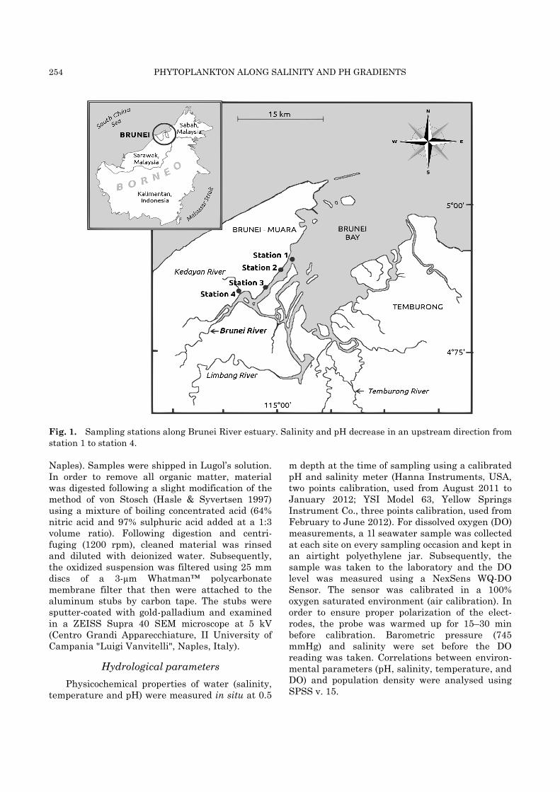
Phytoplankton samples were collected at four stations located along the Brunei River estuary, Chermin Island (S1; 4.927650°N, 115.020406°E), Sungai Bunga (S2; 4.900956°N, 114.998353°E), Pintu Malim (S3; 4.888897°N, 114.979133°E), and Kedayan River-Kiulap (S4; 4.886733°N, 114.936767°E). These were selected to represent a strong gradient of pH and salinity, both decreasing in an upstream direction from S1 to S4 (Fig. 1). Samples were taken at 1- to 3-week intervals between August 2011 and June 2012. Heavy rainfall associated with the Asian monsoons (north-eastern monsoon, NEM, from November to March; south-western monsoon, SWM, from May to September), as well as the dry inter-monsoon periods (April and October), significantly affect the local conditions, bringing droughts and flooding alternately (Adam A., personal observations).

Phytoplankton samples were collected by towing a plankton net (20 µm mesh) behind a small boat ca. 0.5 m under the water surface. On each sampling occasion (18 in total), the same procedure was carried out for 3 min at a constant speed (2 ms–1). Subsequently, collected material was concentrated, transferred into 100 ml containers, and preserved with Lugol’s iodine solution. All sampling took place during the daytime, at the same tidal level (just after high tide). Tidal levels were estimated using TideComp v.7.04 (Pangolin, Bristol, UK) software.

Sedgewick-Rafter counting slides were used for phytoplankton identification and quantification. Prior to observation the samples were homo-genised by gently agitating the sample bottle. From a well-mixed sample, 1 ml was dispensed into the counting cell and viewed under a compound microscope at 40x and 100x magni-fications. This procedure was repeated three times and the final result was expressed as the mean value of the three counts. Collected phytoplankton were identified to the lowest taxonomic level possible using relevant references (e.g. Ehrenberg 1844; Lauder 1864; Schmidt 1874, 1878, 1888, 1890, 1892, 1893; Shirota 1966; Tomas 1997). Scanning electron microscopy of phytoplankton samples was undertaken in Italy (II University of


Fig. 1. Sampling stations along Brunei River estuary. Salinity and pH decrease in an upstream direction from

station 1 to station 4.

Naples). Samples were shipped in Lugol’s solution. In order to remove all organic matter, material was digested following a slight modification of the method of von Stosch (Hasle & Syvertsen 1997) using a mixture of boiling concentrated acid (64% nitric acid and 97% sulphuric acid added at a 1:3 volume ratio). Following digestion and centri-fuging (1200 rpm), cleaned material was rinsed and diluted with deionized water. Subsequently, the oxidized suspension was filtered using 25 mm discs of a 3-µm Whatman™ polycarbonate membrane filter that then were attached to the aluminum stubs by carbon tape. The stubs were sputter-coated with gold-palladium and examined in a ZEISS Supra 40 SEM microscope at 5 kV (Centro Grandi Apparecchiature, II University of Campania "Luigi Vanvitelli", Naples, Italy).

Hydrological parameters

Physicochemical properties of water (salinity, temperature and pH) were measured in situ at 0.5

m depth at the time of sampling using a calibrated pH and salinity meter (Hanna Instruments, USA, two points calibration, used from August 2011 to January 2012; YSI Model 63, Yellow Springs Instrument Co., three points calibration, used from February to June 2012). For dissolved oxygen (DO) measurements, a 1l seawater sample was collected at each site on every sampling occasion and kept in an airtight polyethylene jar. Subsequently, the sample was taken to the laboratory and the DO level was measured using a NexSens WQ-DO Sensor. The sensor was calibrated in a 100% oxygen saturated environment (air calibration). In order to ensure proper polarization of the elect-rodes, the probe was warmed up for 15–30 min before calibration. Barometric pressure (745 mmHg) and salinity were set before the DO reading was taken. Correlations between environ-mental parameters (pH, salinity, temperature, and DO) and population density were analysed using SPSS v. 15.

MAJEWSKA et al. 255

Table 1. Plankton taxa found in the Brunei River Estuary.

Class Family Genera and Species

Bacillariophyceae Achanthaceae Achnanthes sp

Amphipleuraceae Amphiprora sp.

Bacillariaceae Nitzschia longissima (Brébisson) Ralfs

Nitzschia spp.

Pseudo-nitzschia sp.

Biddulphiaceae Biddulphia mobiliensis (J.W. Bailey) Grunow

Biddulphia sinensis Greville

Chaetocerotaceae Bacteriastrum varians Lauder

Bacteriastrum spp.

Chaetoceros danicus Cleve

Chaetoceros peruvianus Brightwell

Chaetoceros rostratus Ralfs

Chaetoceros spp.

Coscinodiscaceae Coscinodiscus jonesianus (Greville) Ostenfeld

Coscinodiscus obscurus A. Schmidt

Coscinodiscus radiatus Ehrenberg

Coscinodiscus wailesii Gran & Angst

Coscinodiscus spp.

Hemiaulaceae Hemiaulus sp.

Leptocylindraceae Corethron sp.

Leptocylindrus sp.

Lithodesmiaceae Ditylum sol Cleve

Melosiraceae Melosira spp.

Naviculaceae Navicula spp.

Pleurosigmataceae Pleurosigma spp.

Rhizosoleniaceae Guinardia striata (Stolterfoth) Hasle

Rhizosolenia alata Brightwell

Rhizosolenia acuminate (H. Peragallo) Gran

Rhizosolenia arafurensis Castracane

Rhizosolenia bergonii H. Peragallo

Rhizosolenia clevei Ostenfeld

Rhizosolenia delicatula Cleve

Rhizosolenia pungens Cleve-Euler

Rhizosolenia stolterfothii H.Peragallo

Stephanodiscaceae Cyclotella litoralis Lange & Syvertsen

Cyclotella meneghiniana Kützing

Surirellaceae Surirella fastuosa Ehrenberg

Thalassionemaceae Thalassionema frauenfeldii (Grunow) Tempère & Peragallo

Thalassionema nitzchioides (Grunow) Mereschkowsky

Thalassiosiraceae Thalassionema sp.

Thalassiosira nanolineata (A.Mann) Fryxell & Hasle

Thalassiosira spp.

Triceratiaceae Triceratium sp.

Contd...


Table 1. Continued.

Class Family Genera and Species

Dinophyceae Ceritiaceae Ceratium furca (Ehrenberg) Claparède & Lachmann

Ceratium fusus (Ehrenberg) Dujardin

Ceratium trichoceros (Ehrenberg) Kofoid

Ceratium tripos (O.F. Müller) Nitzsch

Ceratium massiliense (Gourret) Karsten

Dinophysiaceae Dinophysis acuta Ehrenberg

Diplopsaliaceae Dinophysis caudata Saville-Kent

Preperidinium meunieri (Pavillard) Elbrächter

Gonyaulacaceae Pyrodinium bahamense var. compressum (Böhm)

Steidinger, Tester & F.J.R. Taylor

Peridiniaceae Peridinium spp.

Prorocentraceae Prorocentrum micans Ehrenberg

Prorocentrum granile Schütt

Protoperidiniaceae Protoperidinium pellucidum Bergh

Protoperidinium crassipes (Kofoid) Balech

Spirotrichea Codonellidae Protoperidinium sp.

Codonella spp.

Statistical analyses

Statistical analyses were performed using PAST 2.17b (Hammer et al. 2001), PRIMER Ver. 5 (Clark & Warwick 2001), and Canoco 5 (ter Braak & Šmilauer 2012) software. Although taxa were identified to the lowest taxonomic level possible, further analyses were performed on generic-level data to avoid detection of false patterns due to potential misidentification. A similarity percen-tage analysis (SIMPER) was run to identify phytoplankton taxa responsible for the similarity within groups. To evaluate the relationships between the phytoplankton communities and measured environmental variables, a constrained ordination method was used. Prior to this analysis, an unconstrained unimodal ordination (detrended correspondence analysis, DCA) was performed and the lengths of its ordination axes were measured. On this basis (the longest axis = 2.4 turnover units) the linear method was selected as the most appropriate for the analysed dataset (Šmilauer & Lepš 2014). Subsequently, redundancy analysis (RDA) and partial RDA were performed on log-transformed abundance data. A Monte Carlo permutation test was used to test the significance of the axes (4999 permutations, P < 0.05). In order to select the best subset of the chosen environ-mental variables to summarize the variation in phytoplankton composition, interactive forward

selection was performed. The conditional and simple effects of individual explanatory variables upon the compositional data were assessed using a variation partitioning procedure (Legendre 2007). To visualize the relation of number of taxa found to different pH levels measured at the sampling sites, a Generalized Additive Model (GAM) was used (Šmilauer & Lepš 2014). GAM is a flexible statistical method able to relatively precisely characterize nonlinear contributions of the selected predictor and thus help to better under-stand the interactive behaviour of different variables (Hastie & Tibshirani 1990).

Results

Phytoplankton community

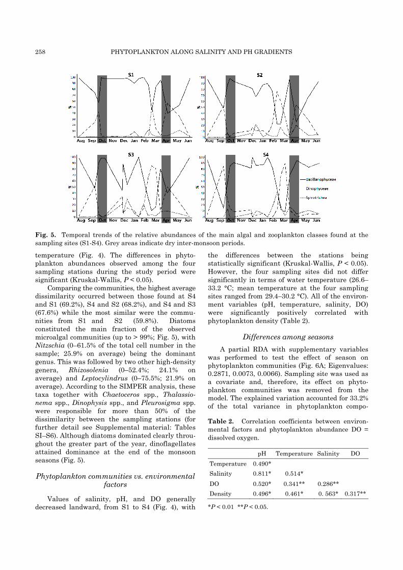
A total of 25 microalgal families were found in the Sungai Brunei estuary area during the period of study, with 22 genera of diatoms, seven of dinoflagellates and one family of ciliates (Table 1, Figs. 2–3). In terms of phytoplankton abundance, the highest density was recorded at S3 (time-averaged mean: 1251 cells ml–1 ± 2544), followed by S2 (1119 cells ml–1 ± 2197), S1 (437 cells ml–1 ± 744) and lastly S4 (118 cells ml–1 ± 265). Generally, the highest phytoplankton densities (up to 9107 cells ml–1, S3) were observed in August and October, which coincided with increases in pH, salinity, and

MAJEWSKA et al. 257

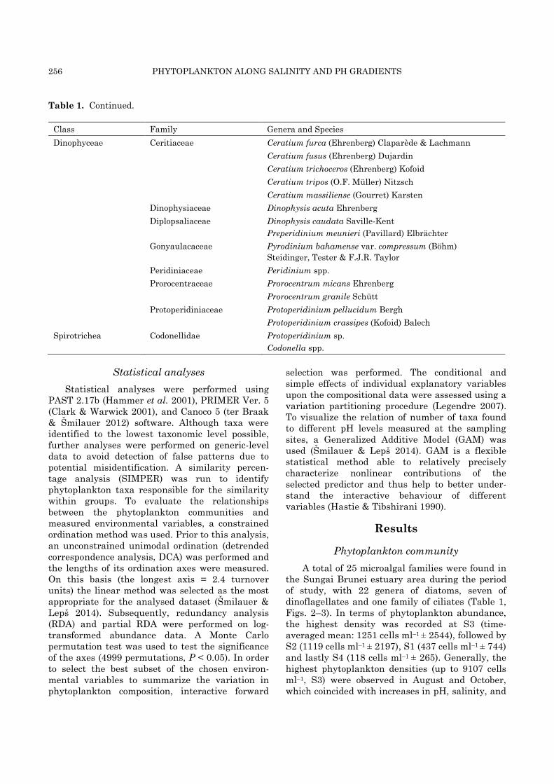
Fig. 2. LM and SEM images of selected diatoms

found in Brunei River estuary. a, b Bacteriastrum sp.

c, d. Coscinodiscus sp. e, f. Pleurosigma sp. g, h.

Cyclotella litoralis. Scale bars: a, b, g, h = 20 µm, c–f

= 10 µm.

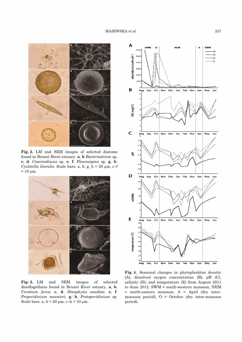
Fig. 3. LM and SEM images of selected

dinoflagellates found in Brunei River estuary. a, b.

Ceratium furca. c, d. Dinophysis caudata. e, f.

Preperidinium meunieri, g, h. Protoperidinium sp.

Scale bars: a, b = 20 µm, c–h = 10 µm.

Fig. 4. Seasonal changes in phytoplankton density

(A), dissolved oxygen concentration (B), pH (C),

salinity (D), and temperature (E) from August 2011

to June 2012. SWM = south-western monsoon, NEM

= north-eastern monsoon, A = April (dry inter-

monsoon period), O = October (dry inter-monsoon

period).


Fig. 5. Temporal trends of the relative abundances of the main algal and zooplankton classes found at the

sampling sites (S1-S4). Grey areas indicate dry inter-monsoon periods.

temperature (Fig. 4). The differences in phyto-plankton abundances observed among the four sampling stations during the study period were significant (Kruskal-Wallis, P < 0.05).

Comparing the communities, the highest average dissimilarity occurred between those found at S4 and S1 (69.2%), S4 and S2 (68.2%), and S4 and S3 (67.6%) while the most similar were the commu-nities from S1 and S2 (59.8%). Diatoms constituted the main fraction of the observed microalgal communities (up to > 99%; Fig. 5), with Nitzschia (0–61.5% of the total cell number in the sample; 25.9% on average) being the dominant genus. This was followed by two other high-density genera, Rhizosolenia (0–52.4%; 24.1% on average) and Leptocylindrus (0–75.5%; 21.9% on average). According to the SIMPER analysis, these taxa together with Chaetoceros spp., Thalassio-nema spp., Dinophysis spp., and Pleurosigma spp. were responsible for more than 50% of the dissimilarity between the sampling stations (for further detail see Supplemental material: Tables SI–S6). Although diatoms dominated clearly throu-ghout the greater part of the year, dinoflagellates attained dominance at the end of the monsoon seasons (Fig. 5).

Phytoplankton communities vs. environmental factors

Values of salinity, pH, and DO generally decreased landward, from S1 to S4 (Fig. 4), with

the differences between the stations being statistically significant (Kruskal-Wallis, P < 0.05). However, the four sampling sites did not differ significantly in terms of water temperature (26.6–33.2 °C; mean temperature at the four sampling sites ranged from 29.4–30.2 °C). All of the environ-ment variables (pH, temperature, salinity, DO) were significantly positively correlated with phytoplankton density (Table 2).

Differences among seasons

A partial RDA with supplementary variables was performed to test the effect of season on phytoplankton communities (Fig. 6A; Eigenvalues: 0.2871, 0.0073, 0.0066). Sampling site was used as a covariate and, therefore, its effect on phyto-plankton communities was removed from the model. The explained variation accounted for 33.2% of the total variance in phytoplankton compo-

Table 2. Correlation coefficients between environ-

mental factors and phytoplankton abundance DO =

dissolved oxygen.

pH Temperature Salinity DO

Temperature 0.490*

Salinity 0.811* 0.514*

DO 0.520* 0.341** 0.286**

Density 0.496* 0.461* 0. 563* 0.317**

*P < 0.01 **P < 0.05.

MAJEWSKA et al. 259

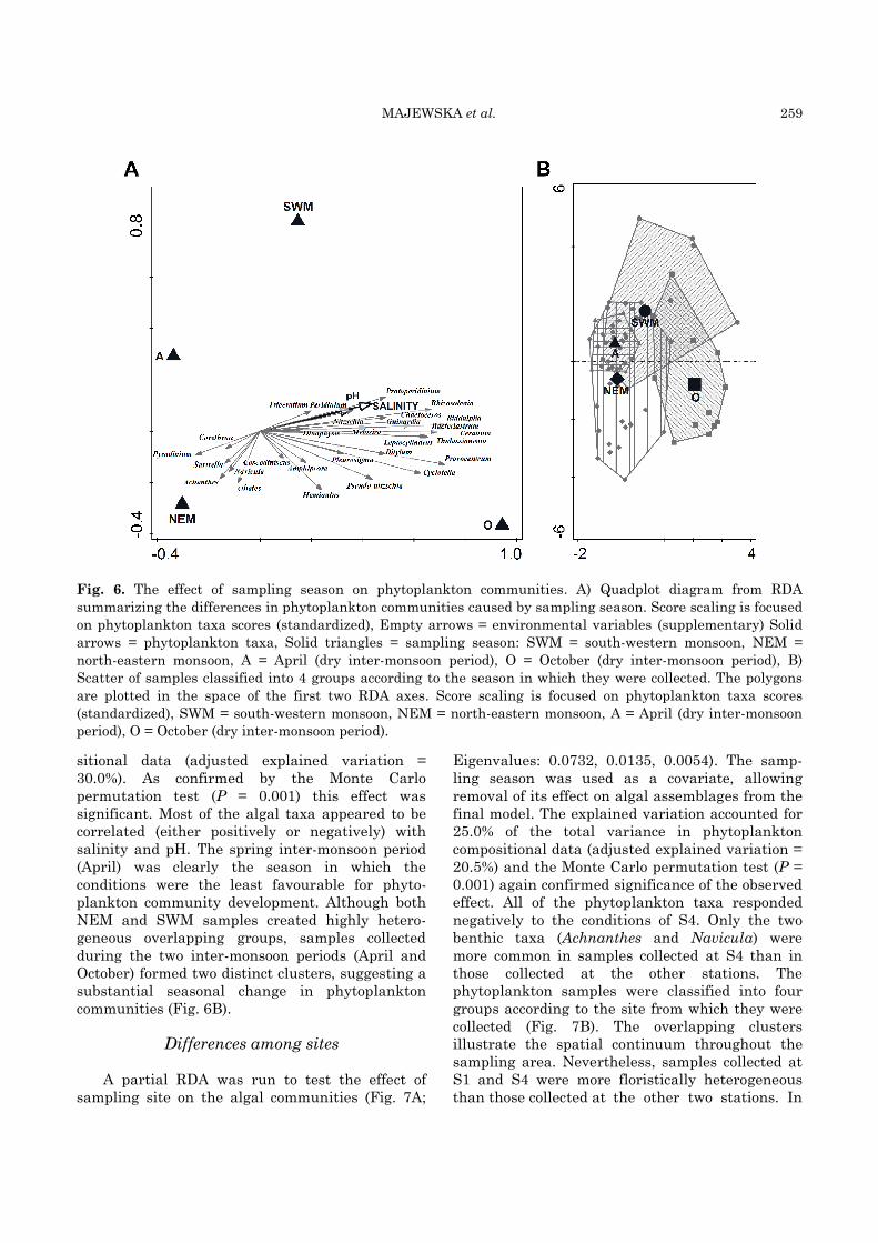
Fig. 6. The effect of sampling season on phytoplankton communities. A) Quadplot diagram from RDA

summarizing the differences in phytoplankton communities caused by sampling season. Score scaling is focused

on phytoplankton taxa scores (standardized), Empty arrows = environmental variables (supplementary) Solid

arrows = phytoplankton taxa, Solid triangles = sampling season: SWM = south-western monsoon, NEM =

north-eastern monsoon, A = April (dry inter-monsoon period), O = October (dry inter-monsoon period), B)

Scatter of samples classified into 4 groups according to the season in which they were collected. The polygons

are plotted in the space of the first two RDA axes. Score scaling is focused on phytoplankton taxa scores

(standardized), SWM = south-western monsoon, NEM = north-eastern monsoon, A = April (dry inter-monsoon

period), O = October (dry inter-monsoon period).

sitional data (adjusted explained variation = 30.0%). As confirmed by the Monte Carlo permutation test (P = 0.001) this effect was significant. Most of the algal taxa appeared to be correlated (either positively or negatively) with salinity and pH. The spring inter-monsoon period (April) was clearly the season in which the conditions were the least favourable for phyto-plankton community development. Although both NEM and SWM samples created highly hetero-geneous overlapping groups, samples collected during the two inter-monsoon periods (April and October) formed two distinct clusters, suggesting a substantial seasonal change in phytoplankton communities (Fig. 6B).

Differences among sites

A partial RDA was run to test the effect of sampling site on the algal communities (Fig. 7A;

Eigenvalues: 0.0732, 0.0135, 0.0054). The samp-ling season was used as a covariate, allowing removal of its effect on algal assemblages from the final model. The explained variation accounted for 25.0% of the total variance in phytoplankton compositional data (adjusted explained variation = 20.5%) and the Monte Carlo permutation test (P = 0.001) again confirmed significance of the observed effect. All of the phytoplankton taxa responded negatively to the conditions of S4. Only the two benthic taxa (Achnanthes and Navicula) were more common in samples collected at S4 than in those collected at the other stations. The phytoplankton samples were classified into four groups according to the site from which they were collected (Fig. 7B). The overlapping clusters illustrate the spatial continuum throughout the sampling area. Nevertheless, samples collected at S1 and S4 were more floristically heterogeneous than those collected at the other two stations. In


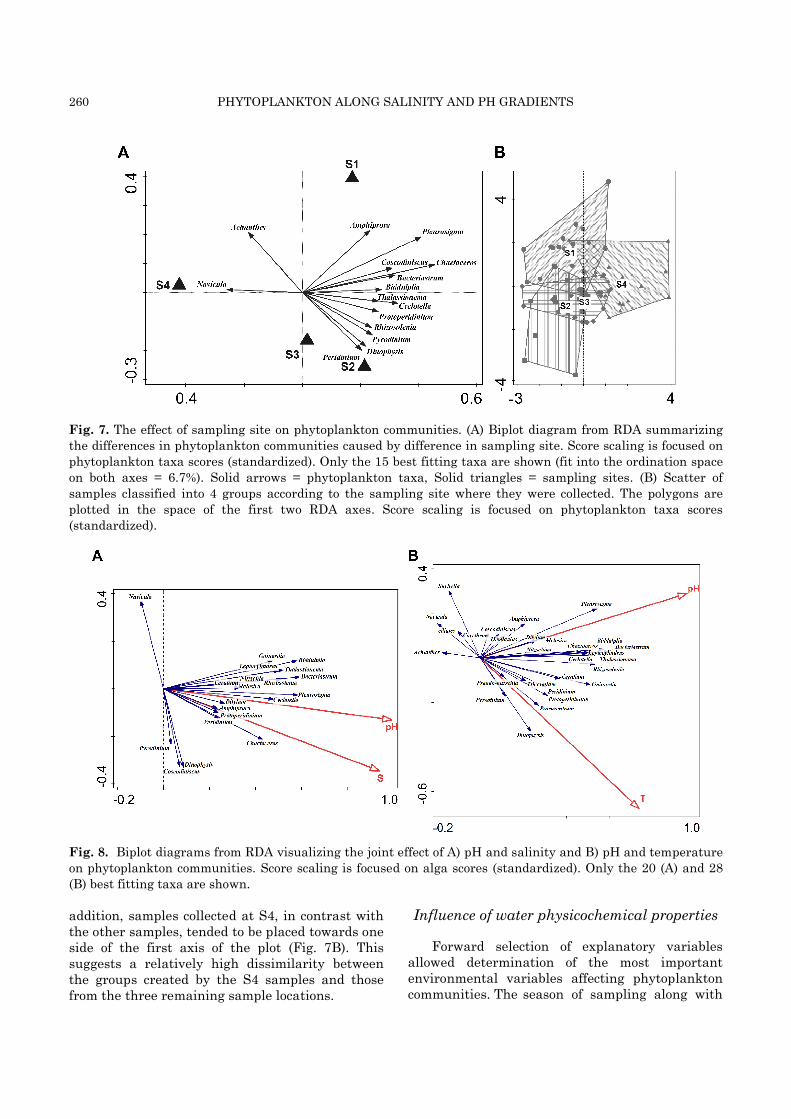
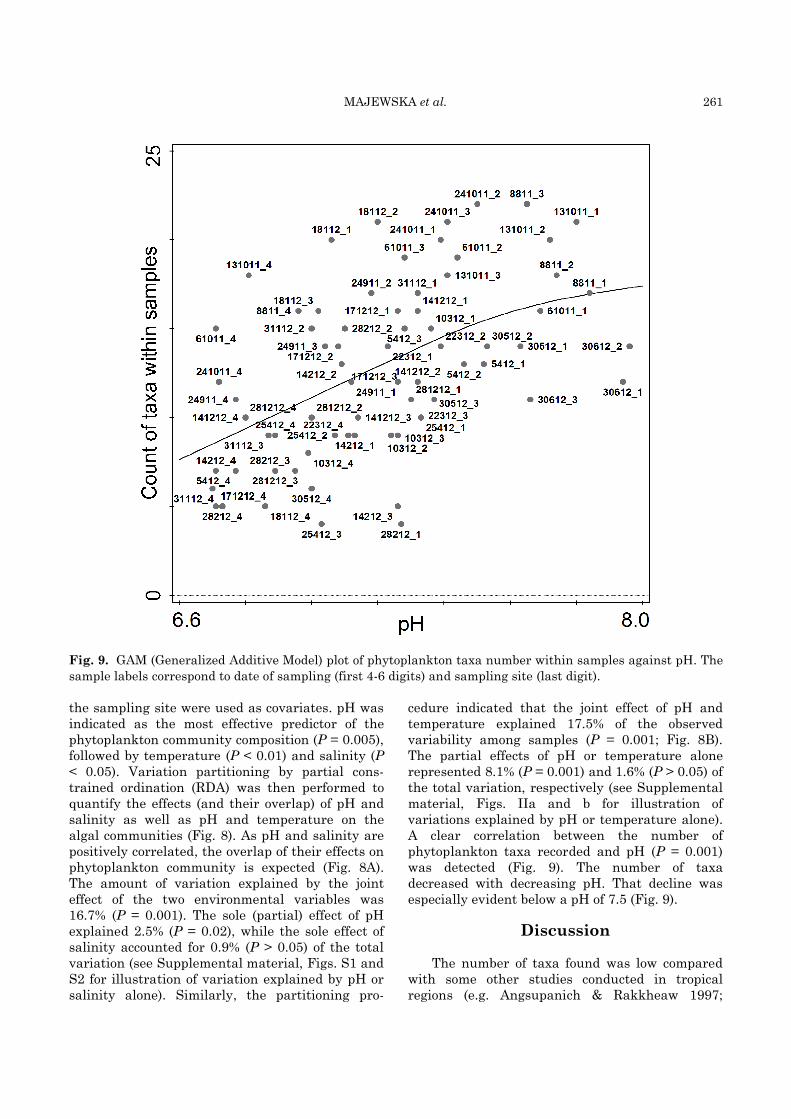
Fig. 7. The effect of sampling site on phytoplankton communities. (A) Biplot diagram from RDA summarizing

the differences in phytoplankton communities caused by difference in sampling site. Score scaling is focused on

phytoplankton taxa scores (standardized). Only the 15 best fitting taxa are shown (fit into the ordination space

on both axes = 6.7%). Solid arrows = phytoplankton taxa, Solid triangles = sampling sites. (B) Scatter of

samples classified into 4 groups according to the sampling site where they were collected. The polygons are

plotted in the space of the first two RDA axes. Score scaling is focused on phytoplankton taxa scores

(standardized).

Fig. 8. Biplot diagrams from RDA visualizing the joint effect of A) pH and salinity and B) pH and temperature

on phytoplankton communities. Score scaling is focused on alga scores (standardized). Only the 20 (A) and 28

(B) best fitting taxa are shown.

addition, samples collected at S4, in contrast with the other samples, tended to be placed towards one side of the first axis of the plot (Fig. 7B). This suggests a relatively high dissimilarity between the groups created by the S4 samples and those from the three remaining sample locations.

Influence of water physicochemical properties

Forward selection of explanatory variables allowed determination of the most important environmental variables affecting phytoplankton communities. The season of sampling along with

MAJEWSKA et al. 261

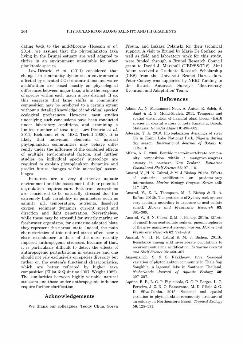
Fig. 9. GAM (Generalized Additive Model) plot of phytoplankton taxa number within samples against pH. The

sample labels correspond to date of sampling (first 4-6 digits) and sampling site (last digit).

the sampling site were used as covariates. pH was indicated as the most effective predictor of the phytoplankton community composition (P = 0.005), followed by temperature (P < 0.01) and salinity (P < 0.05). Variation partitioning by partial cons-trained ordination (RDA) was then performed to quantify the effects (and their overlap) of pH and salinity as well as pH and temperature on the algal communities (Fig. 8). As pH and salinity are positively correlated, the overlap of their effects on phytoplankton community is expected (Fig. 8A). The amount of variation explained by the joint effect of the two environmental variables was 16.7% (P = 0.001). The sole (partial) effect of pH explained 2.5% (P = 0.02), while the sole effect of salinity accounted for 0.9% (P > 0.05) of the total variation (see Supplemental material, Figs. S1 and S2 for illustration of variation explained by pH or salinity alone). Similarly, the partitioning pro-

cedure indicated that the joint effect of pH and temperature explained 17.5% of the observed variability among samples (P = 0.001; Fig. 8B). The partial effects of pH or temperature alone represented 8.1% (P = 0.001) and 1.6% (P > 0.05) of the total variation, respectively (see Supplemental material, Figs. IIa and b for illustration of variations explained by pH or temperature alone). A clear correlation between the number of phytoplankton taxa recorded and pH (P = 0.001) was detected (Fig. 9). The number of taxa decreased with decreasing pH. That decline was especially evident below a pH of 7.5 (Fig. 9).

Discussion

The number of taxa found was low compared with some other studies conducted in tropical regions (e.g. Angsupanich & Rakkheaw 1997;


Lueangthuwapranit et al. 2011; Su et al. 2004). Su et al. (2004) reported 64 phytoplankton species (including diatoms, dinoflagellates, chlorophytes, and cyanobacteria) in their study of Tapong Bay (Taiwan) and Lueangthuwapranit et al. (2011) observed 74 genera from 6 divisions in samples taken from the Na Thap River estuary (Thailand). Although we cannot exclude these differences being influenced by methodology, we do not consider this is sufficient to explain the generally low functional diversity observed in phytoplankton from the Brunei River estuary. Whereas the phytoplankton communities present at the four sampling stations differed significantly in terms of both algal abundance and composition, the main differences were not caused by presence or absence of strictly stenohaline taxa, but rather by the dominance of the main common diatom and dinoflagellate taxa changing along the pH and salinity gradients.

As noted in several studies (Jacobsen & Andersen 1994; Loverde-Oliveira et al. 2009; Muylaert & Sabbe 1999), many dinoflagellate species may have mixo- or heterotrophic nutrition, which favours their survival in highly turbid conditions. Furthermore, it has been suggested that a higher carbon: chlorophyll ratio in dinofla-gellates compared with diatoms may be responsible for their faster growth in conditions of lower pH and elevated CO2 concentration (Low-Décarie et al. 2011; Tortell et al. 2008). Many diatom species are known to be relatively resistant to a moderate decrease in water pH (up to 0.3 pH units), but their numbers reduce drastically with any further decrease of pH (Geelen & Leuven 1986, and references therein; Majewska, personal observations). Also, species within some diatom genera (e.g. Cyclotella) are known to have clear heterotrophic capabilities, which enable them to survive in low-light conditions (Lylis & Trainer 1973).

The outcomes of several statistical models indicated that the communities investigated were strongly influenced by season (explaining ca. 30% of the total variance in phytoplankton compo-sitional data) and by the set of factors specifically related to each sampling station (ca. 20% of the total variance). pH appeared to have a stronger influence on phytoplankton assemblages than salinity, temperature, or dissolved oxygen. Although pH is strongly correlated with salinity (Hansen 2002; Zhou & Rowland 1997), in many cases its effect when considered alone was opposite to that of salinity, i.e. taxa associated with lower

salinity levels appeared to prefer higher pH conditions, and vice versa, when the shared effect of pH and salinity was excluded from the model. A large majority of the taxa had their local optima in stations characterized by relatively high pH values, while the GAM plot illustrates the positive correlation of pH and the number of taxa found in the samples. Other studies on tropical estuarine phytoplankton have reported similar trends. Madhu et al. (2007) observed that diversity of phytoplankton in Cochin backwaters (southwest India) decreased during the monsoon season when heavy rainfalls caused decrease in both salinity and pH, whereas Costa et al. (2001), who examined phytoplankton in the Paraiba do Sul River estuary (Brazil), observed that the highest biodiversity was associated with the highest pH and high water residence, and concluded that freshwater discharges controlled both species composition and their biomass.

Minima in phytoplankton diversity and abundance were found at the most landward station, S4, indicating the least favourable conditions for microalgal growth. Although most of the genera were present in different seasons and in various numbers at all four stations, genera such as Corethron, Cyclotella, Guinardia, and Triceratium were never present in samples from S4. A combination of extreme turbidity, resulting in severe light limitation, distinctly lower salinity, pH, and DO values in the proximity of large urban areas (e.g. Kiulap, Gadong, water villages along the estuary) could have affected local phyto-plankton markedly more than at the more seaward locations. A relatively high contribution of typically benthic taxa (Achnanthes spp., Navicula spp.) to the phytoplankton found in S4 samples indicated significant exchange with the benthic communities and a high level of physical disturbance (turbidity, river runoff; Aquino et al. 2015), which might also limit the development of phytoplankton assemblages (Adesalu 2010; Cloern 1987; Muylaert & Sabbe 1999; Palleyi et al. 2008).

Sampling season proved to have a pronounced effect on the estuarine phytoplankton. The RDA models clearly indicated that the dry inter-monsoon period following NEM heavy rainfalls was the least suitable for the phytoplankton development. The two monsoon seasons resulted in changes in microalgal communities in qualitatively and quantitatively distinct ways. The highest abundances (up to 9107 cells ml–1) were associated with the SWM season and not with NEM, in which a series of the heaviest rainfalls occurred.

MAJEWSKA et al. 263

Fluctuations in water parameters observed during the NEM season were an effect of turbulent events and high water mixing caused by both heavy rainfalls and north-eastern winds favouring marine water intrusions into the estuary. Wet season and other rainfall events may promote phytoplankton blooms through the leaching of biogenic substances from the adjacent land and the large influx of riverine water highly enriched in organic matter and nutrients (Angsupanich & Rakkheaw 1997; Gameiro et al. 2004; Jackson et al. 1987; Lueangthuwapranit et al. 2011; Mallin et al. 1993). In addition, algal growth is enhanced by lower tidal variation associated with the monsoon seasons (Palleyi et al. 2008), with tides being recognised as possibly one of the most important factors for local phytoplankton development (Lueangthuwapranit et al. 2011; Su et al. 2004; Wan Maznah et al. 2016). In some cases, however, extremely intense rainfall events may negatively affect phytoplankton communities by increasing turbidity (Mallin et al. 1993) and by introducing into the aquatic systems an excessive amount of acid drainage water and heavy metals that are easily leached from the soil in the low pH environment (Green & Barnes 2010; Macdonald et al. 2007; Russel & Helmke 2002). Strongly geologically originated ASS are found in the vicinity of the Sungai Brunei estuary (Bolhuis et al. 2014; Grealish & Fitzpatrick 2013) and the risk of these becoming increasingly damaging to the environment depends greatly on local management and land use practices. Appropriate management practices are not always well understood and it is highly probable that intense leaching during the wet seasons causes a serious threat to water quality and aquatic life (e.g. Dent & Pons 1995; Sammut et al. 1995). Adam et al. (2011) working in eastern Malaysia and Tan et al. (2006) in the eastern Malacca Straits reported that intense phytoplankton blooms were observed mainly during the NEM. The monsoon influence was associated with strong north-east winds respon-sible for extensive mixing of the water column. These studies, however, were focused on marine habitats that are only minimally influenced by freshwater and it is unclear how applicable their findings are to the estuarine environment.

A smaller peak in algal abundance was also observed during the dry period in October. The phenomenon was associated with an increase in DO, salinity, and pH and a decrease in temperature suggesting a higher inflow of saline water into the river. Similar changes in hydro-

logical conditions were less pronounced in April when the heavy winter rains subsided, and this was not followed by an increase in plankton abundance. Costa et al. (2009) observed that a strong influence of marine waters on the Paraiba do Sul River estuary (Brazil) caused increase in both phytoplankton biomass and species richness and that a high river flow and turbidity supported mainly fast growing nanoplankton (< 20 µm) or some large diatom cells able to remain suspended even in shallow and turbulent waters. In our studies phytoplankton samples were collected with a 20 µm mesh and it is likely that any peak in nanoplankton abundance would not have been detected with the sampling methodology used.

Sampling season, site, and water pH explained ca. 60% of the observed variation in the phyto-plankton data obtained. However, we recognise that variables not included in these analyses might also significantly affect the communities. This may be inferred from the low eigenvalue of the second axis of the RDA, which was weakly correlated with the selected environmental variables. For instance, high nutrient concen-trations often found in the upper part of the estuary (Pintu Malim - Sungai Kedayan), might counter the negative effect of low pH (Jalal et al. 2011). In this region, nutrient levels are likely to be elevated through sewage treatment activities at Pintu Malim, release of organic materials from Kampong Ayer, small-scale aquaculture facilities, and the effect of Sungai Kedayan inflow, which carries water from a large urbanized area. According to Biswas et al. (2011) diatoms may benefit from elevated CO2 concentrations in the estuarine water, but only if the nutrient levels are not a limiting factor. Amongst other potentially important influences, grazing and other biological factors (e.g. parasitism) have been suggested to play an important role in phytoplankton dynamics (Canter & Lund 1953; Muylaert & Sabbe 1999).

Although the acute temporal variability in acidification that coincides with seasonal flooding is assumed to relate largely to ASS inflows, finer temporal scale tidal fluctuations in pH during inter-monsoons are more likely to be associated with the combination of a lowered buffering capacity, microbial decomposition, and pCO2 saturation in the upper estuarine reaches (Bolhuis et al. 2014; Hossain et al. 2014; Proum S. un-published). As many of the processes involved in this complex acidification are natural, with potentially acid-generating geological formations and biological communities (mangroves) probably


dating back to the mid-Miocene (Hossain et al. 2014), we assume that the phytoplankton taxa living in the Brunei estuary are well adapted to thrive in an environment unsuitable for other planktonic species.

Low-Décarie et al. (2011) considered that changes in community dynamics in environments affected by elevated CO2 concentrations and water acidification are based mostly on physiological differences between major taxa, while the response of species within each taxon is less distinct. If so, this suggests that large shifts in community composition may be predicted to a certain extent without a detailed knowledge of individual species’ ecological preferences. However, most studies underlying such conclusions have been conducted under laboratory conditions, and examining a limited number of taxa (e.g. Low-Décarie et al. 2011; Richmond et al. 1982; Tortell 2000). It is likely that individual elements of natural phytoplankton communities may behave diffe-rently under the influence of the combined effects of multiple environmental factors, and further studies on individual species’ autecology are required to explain phytoplankton dynamics and predict future changes within microalgal assem-blages.

Estuaries are a very distinctive aquatic environment and the assessment of their potential degradation requires care. Estuarine ecosystems are considered to be naturally stressed due the extremely high variability in parameters such as salinity, pH, temperature, nutrients, dissolved oxygen, sediment dynamics, current speed and direction and light penetration. Nevertheless, while these may be stressful for strictly marine or freshwater organisms, for estuarine-adapted biota they represent the normal state. Indeed, the main characteristics of this natural stress often bear a close resemblance to those of the more recently imposed anthropogenic stressors. Because of that, it is particularly difficult to detect the effects of anthropogenic perturbations in estuaries and one should not rely exclusively on species diversity but rather on the system’s functional characteristics, which are better reflected by higher taxa composition (Elliot & Quintino 2007; Wright 1982). The similarities between highly variable natural stressors and those under anthropogenic influence require further clarification.

Acknowledgements

We thank our colleagues: Teddy Chua, Sorya

Proum, and Lukasz Polanski for their technical support. A visit to Brunei by Mario De Stefano, as well as field and laboratory work for this study, were funded through a Brunei Research Council grant to David J. Marshall (UBD/S&T/16). Aimi Adam received a Graduate Research Scholarship (GRS) from the Universiti Brunei Darussalam. Peter Convey was supported by NERC funding to the British Antarctic Survey’s ‘Biodiversity Evolution and Adaptation’ Team.

References

Adam, A., N. Mohammad-Noor, A. Anton, E. Saleh, S.

Saad & R. S. Muhd-Shaleh. 2011. Temporal and

spatial distribution of harmful algal bloom (HAB)

species in coastal waters of Kota Kinabalu, Sabah,

Malaysia. Harmful Algae 10: 495–502.

Adesalu, T. A. 2010. Phytoplankton dynamics of river

Oli in Kainji Lake National Park, Nigeria during

dry season. International Journal of Botany 6:

112–116.

Alfaro, A. C. 2006. Benthic macro-invertebrate commu-

nity composition within a mangrove/seagrass

estuary in northern New Zealand. Estuarine

Coastal and Shelf Science 66: 97–110.

Amaral, V., H. N. Cabral, & M. J. Bishop. 2012a. Effects

of estuarine acidification on predator-prey

interactions. Marine Ecology Progress Series 445:

117–127.

Amaral, V., E. L. Thompson, M. J. Bishop & D. A.

Raftos. 2012b. The proteomes of Sydney rock oysters

vary spatially according to exposure to acid sulfate

runoff. Marine and Freshwater Research 63:

361–369.

Amaral, V., H. N. Cabral & M. J. Bishop. 2011a. Effects

of runoff from acid-sulfate soils on pneumatophores

of the grey mangrove Avicennia marina. Marine and

Freshwater Research 62: 974–979.

Amaral, V., H. N. Cabral & M. J. Bishop. 2011b.

Resistance among wild invertebrate populations to

recurrent estuarine acidification. Estuarine Coastal

and Shelf Science 93: 460–467.

Angsupanich, S. & S. Rakkheaw. 1997. Seasonal

variation of phytoplankton community in Thale Sap

Songkhla, a lagoonal lake in Southern Thailand.

Netherlands Journal of Aquatic Ecology 30:

297–307.

Aquino, E. P., L. G. P. Figueiredo, G. C. P. Borges, L. C.

Ferreira, J. Z. D. O. Passavante, M. D. Glόria & G.

D. Silva-Cunha. 2015. Seasonal and spatial

variation in phytoplankton community structure of

an estuary in Northeastern Brazil. Tropical Ecology

56: 125–131.

MAJEWSKA et al. 265

Berge, T., N. Daugbjerg, B. B. Andersen & P. J. Hansen.

2010. Effect of lowered pH on marine phytoplankton

growth rates. Marine Ecology Progress Series 416:

79–91.

Biswas H., A. Cros, K. Yadav, V. V. Ramana, V. R.

Prasad, T. Acharyya & P. V. R. Babu. 2011. The

response of a natural phytoplankton community

from the Godavari River Estuary to increasing CO2

concentration during the pre-monsoon period.

Journal of Experimental Marine Biology and

Ecology 407: 284–293.

Bolhuis, H., H. Schluepmann, J. Kristalijn, Z. Sulaiman

& D. J. Marshall. 2014. Molecular analysis of

bacterial diversity in mudflats along the salinity

gradient of an acidified tropical Bornean estuary

(South East Asia). Aquatic Biosystems 10: 10.

doi:10.1186/2046-9063-10-10.

Boynton, W. R., W. M. Kemp & C. W. Keefe. 1982. A

comparative analysis of nutrients and other factors

influencing estuarine phytoplankton production.

pp. 69–90 In: V. S. Kennedy (ed.) Estuarine Com-

parisons. Academic Press, New York.

Brading, P., M. E. Warner, P. Davey, D. J. Smith, E. P.

Achterberg & D. J. Suggett. 2011. Differential

effects of ocean acidification on growth and photo-

synthesis among phylotypes of Symbiodinium

(Dinophyceae). Limnology and Oceanography 56:

927–938.

Canter, H. M. & J. W. G. Lund. 1953. Studies on

plankton parasites: II. The parasitism of diatoms

with special reference to lakes in the English Lake

District. Transactions of the British Mycological

Society 27: 6–93.

Cai, W. J., X. Hu, W. J. Huang, M. C. Murrell, J. C.

Lehrter, S. E. Lohrenz, W.-C. Chou, Z. Weidong, T.

H. James, W. Yongchen et al. 2011. Acidification of

subsurface coastal waters enhanced by eutro-

phication. Nature Geoscience 4: 766–770.

Caldeira, K. & M. E. Wickett. 2003. Oceanography:

anthropogenic carbon and ocean pH. Nature 425:

365.

Cassar, N., E. A. Laws & R. R. Bidigare. 2003.

Bicarbonate uptake by Southern Ocean

phytoplankton. Global Biogeochemical Cycles 18 doi:

10.1029/2003GB002116

Chua, T.-E., L. M. Chou & M. S. M. Sadorra. 1987. The

coastal environmental profile of Brunei Darusslam:

resource assessment and management issues.

ICLARM Technical Report 18. Fisheries Depart-

ment, Ministry of Development, Brunei Darus-

salam.

Cloern, J. E. 1987. Turbidity as a control on

phytoplankton biomass and productivity in

estuaries. Continental Shelf Research 7: 1367–1381.

Cook, F. J., W. Hicks, E. A. Gardner, G. D. Carlin & D.

W. Froggatt. 2000. Export of acidity in drainage

water from acid sulphate soils. Marine Pollution

Bulletin 41: 319–326.

Costa, L. S., V. L. M. Huszar & A. R. Ovalle. 2009.

Phytoplankton functional groups in a tropical

estuary: hydrological control and nutrient limi-

tation. Estuaries and Coasts 32: 508–521.

Costanza, R., R. d’Arge, R. de Groot, S. Farber, M. Grasso,

B. Hannon, K. Limburg, S. Naeem, R. V. Oneill, J.

Paruelo et al. 1997. The value of the world's

ecosystem services and natural capital. Nature 387:

253–260.

Currie, D. 1979. Some aspects of the hydrology of the

Brunei Estuary. Brunei Museum Journal 6:

199–239.

de Jonge, V. N., M. Elliott & E. Orive. 2002. Causes,

historical development, effects and future chal-

lenges of a common environmental problem:

eutrophication. Hydrobiologia 475: 1–19.

Dent, D. L. & L. J. Pons. 1995. A world perspective on

acid sulfate soils. Geoderma 67: 263–276.

Doney, S. C., V. J. Fabry, R. A. Feely & J. A. Kleypas.

2009. Ocean acidification: The other CO2 problem.

Annual Review of Marine Science 1: 169–192.

Dove, M. C. & J. Sammut. 2007. Impacts of estuarine

acidification on survival and growth of Sydney rock

oysters Saccostrea glomerata (Gould 1850). Journal

of Shellfish Research 26: 519–527.

Downing, J. A., M. McClain, R. J. Twilley, M. Melack, J.

Elser, N. N. Rabalais, W. M. Lewis,, R. E. Turner

Jr., J. Corredor, D. Soto et al. 1999. The impact of

accelerating land-use change on the N-cycle of

tropical aquatic ecosystems: current conditions and

projected changes. Biogeochemistry 46: 109–148.

Duarte, C. M., I. E. Hendriks, T. M. Moore, Y. S. Olsen,

A. Steckbauer, L. Ramajo, J. Carstensen, J. A.

Trotter & M. McCulloch. 2013. Is Ocean acidi-

fication an open-ocean syndrome? Understanding

anthropogenic impacts on seawater pH. Estuaries

and Coasts 36: 221–236.

Ehrenberg, C. G. 1844. Mittheilung über 2 neue lager

von Gebirgsmassen aus infusorien als Meeres-

Absatz in Nord Amerika und eine vergleichung

derselben mit den organischen Kreide-Ge-bilden in

Europa und Afrika. Bericht über die zur Bekannt-

machung Geeigneten Verhandlungen der Königl.

Preuss. Akademie Der Wissenschaften zu Berlin

1844: 57–97.

Elliot, M. & V. Quintino. 2007. The Estuarine quality


paradox, environmental homeostasis and the

difficulty of detecting anthropogenic stress in

naturally stressed areas. Marine Pollution Bulletin

54: 640–645.

Fabry, V. J., B. A. Seibel, R. A. Feely & J. C. Orr. 2008.

Impacts of ocean acidification on marine fauna and

ecosystem processes. ICES Journal of Marine

Science: Journal du Conseil 65: 414–432.

Falkowski, P. 2012. Ocean science: The power of

plankton. Nature 483: 17–20.

Feely, R. A., S. R. Alin, J. Newton, C. L. Sabine, M.

Warner, A. Devol, C. Krembs & C. Maloy. 2010. The

combined effects of ocean acidification, mixing, and

respiration on pH and carbonate saturation in an

urbanized estuary. Estuarine Coastal and Shelf

Science 88: 442–449.

Gameiro, C., P. Cartaxana, M. T. Cabrita & V. Brotas.

2004. Variability in chlorophyll and phytoplankton

composition in an estuarine system. Hydrobiologia

525: 113–124.

Gazeau, F., S. Alliouane, C. Bock, L. Bramanti, M. López

Correa, M. Gentile, T. Hirse, H.-O. Pörtner & P.

Ziveri. 2014. Impact of ocean acidification and

warming on the Mediterranean mussel (Mytilus

galloprovincialis). Frontiers in Marine Science 1,

doi: 10.3389/fmars.2014.00062.

Gazeau, F., L. M. Parker, S. Comeau, J.-P. Gattuso, W.

A. O’Connor, S. Martin, H.-O. Pörtner & P. M. Ross.

2013. Impacts of ocean acidification on marine

shelled molluscs. Marine Biology 160: 2207–2245.

Geelen, J. F. M. & R. S. E. W. Leuven. 1986. Impact of

acidification on phytoplankton and zooplankton

communities. Cellular and Molecular Life Sciences

42: 486–494.

Grealish, G. J. & R. W. Fitzpatrick. 2013. Acid sulphate

soil characterization in Negara Brunei Darussalam:

a case study to inform management decisions. Soil

Use Management 29: 432–444.

Green, T. J. & A. C. Barnes. 2010. Reduced salinity, but

not estuarine acidification, is a cause of immune-

suppression in the Sydney rock oyster Saccostrea

glomerata. Marine Ecology Progress Series 402:

161–170.

Hall-Spencer, J. M, R. Rodolfo-Metalpa, S. Martin, E.

Ransome, M. Fine, S. M. Turner, S. J. Rowley, D.

Tedesco & M. C. Buia. 2008. Volcanic carbon dioxide

vents show ecosystem effects of ocean acidification.

Nature 454: 96–99.

Hammer, Ø., D. A. T. Harper & P. D. Ryan. 2001. PAST:

Palaeontology statistical software package for

education and data analysis. Palaeontologia

Electronica 4: 1–9.

Hansen, P. J., 2002. Effect of high pH on the growth and

survival of marine phytoplankton: implications for

species succession. Aquatic Microbial Ecology 28:

279–288.

Hasle, G. R. & E. E. Syvertsen. 1997. Marine diatoms.

In: C. R. Tomas (ed.) Identifying Marine Phyto-

plankton. Academic Press, San Diego, pp. 5–385.

Hasties, T. J. & R. J. Tibshirani. 1990. Generalized

Additive Models. Chapman and Hall, New York.

Hinga, K. R. 2002. Effects of pH on coastal marine

phytoplankton. Marine Ecology Progress Series 238:

281–300.

Hopkinson, C. S., A. E. Giblin, J. Tucker & R. H. Garrit.

1999. Benthic metabolism and nutrient cycling

along an estuarine salinity gradient. Estuaries 22:

863–881.

Hossain, M. B. & D. J. Marshall. 2014. Benthic infaunal

community structuring in an acidified tropical

estuarine system. Aquatic Biosystems 10: 11, doi:

10.1186/2046-9063-10-11.

Hossain, M. B., D. J. Marshall, & V. Senapathi. 2014.

Sediment granulometry and organic matter content

in the intertidal zone of the Sungai Brunei

estuarine system, northwest coast of Borneo.

Carpathian Journal of Earth and Environmental

Sciences 9: 231–239.

Hu, X. & W.-J. Cai. 2013. Estuarine acidification and

minimum buffer zone - A conceptual study. Geo-

physical Research Letters 40: 5176–5181.

Jalal, K. C. A., B. M. Ahmad Azfar, B. Akhbar John & Y.

B. Kamaruzzaman. 2011. Spatial variation and

community composition of phytoplankton along the

Pahang estuary, Malaysia. Asian Journal of Bio-

logical Sciences 4: 468–476.

Jackson, R., P. L. Williams & I. Joint. 1987. Freshwater

phytoplankton in the low salinity region of the River

Tamar Estuary. Estuarine Coastal and Shelf Science

25: 299–311.

Jacobson, D. M. & R. A. Andersen. 1994. The discovery

of mixotrophy in photosynthetic species of Dino-

physis (Dinophyceae): ligh and electron micro-

scopical observations of food vacuoles in Dynophysis

acuminata, D. norvegica and two heterotrophic

dinophysoid dinoflagellates. Phycologia 33: 97–110.

Johnson, V. R., B. D. Russell, K. E. Fabricius, C.

Brownlee & J. M. Hall-Spencer. 2012. Temperate

and tropical brown macroalgae thrive, despite

decalcification, along natural CO2 gradients. Global

Change Biology 18: 2792–2803.

Lauder, H. S. 1864. Remarks on the marine Diato-

maceae found at Hong Kong, with descriptions of

new species. Transactions of the Microscopical

MAJEWSKA et al. 267

Society of London 12: 75–79.

Legendre, P. 2007. Studying beta diversity: ecological

variation partitioning by multiple regression and

canonical analysis. Journal of Plant Ecology 1: 3–8.

Lohbeck, K. T., U. Riebesell & T. B. Reusch. 2012.

Adaptive evolution of a key phytoplankton species to

ocean acidification. Nature Geosciences 5: 346–351.

Longhurst, A., S. Sathyendranath, T. Platt & C.

Caverhill. 1995. An estimate of global primary

production in the ocean from satellite radiometer

data. Journal of Plankton Research 17: 1245–1271.

Loverde-Oliveira, S.M., V. L. Moraes Huszar, N. Mazzeo

& M. Scheffer. 2009. Hydrology-driven regime shifts

in a shallow tropical lake. Ecosystems 12: 807–819.

Low‐Décarie, E., G. F. Fussmann & G. Bell. 2011. The

effect of elevated CO2 on growth and competition in

experimental phytoplankton communities. Global

Change Biology 17: 2525–2535.

Lueangthuwapranit, C., U. Sampantarak & S. Wongsai.

2011. Distribution and abundance of phytoplankton:

Influence of salinity and turbidity gradient in the

Na Thap River, Songkhla Province, Thailand.

Journal of Coastal Research 27: 585–594.

Lylis, J. C. & F. R. Trainor. 1973. The heterotrophic

capabilities of Cyclotella meneghiniana. Journal of

Phycology 9: 365–369.

Macdonald, B. C. T., I. White, M. E. Astrom, A. F.

Keene, M. D. Melville & J. K. Reynolds. 2007.

Discharge of weathering products from acid sulfate

soils after a rainfall event, Tweed River, eastern

Australia. Applied Geochemistry 22: 2695–2705.

Madhu, N. V., R. Jyothibabu, K. K. Balachandran, U. K.

Honey, G. D. Martin, J. G. Vijay, C. A. Shiyas, G. V.

M. Gupta & C. T. Achuthankutty. 2007. Monsoonal

impact on planktonic standing stock and abundance

in a tropical estuary (Cochin backwaters-India).

Estuarine Coastal and Shelf Science 73: 54–64.

Majewska, R., P. Lemke, P., A. Zgrundo & M. De

Stefano. 2012. Benthic diatoms of the Vistula River

estuary (Northern Poland) - seasonality, substrata

preferences, and the influence of water chemistry.

Phycological Research 60: 1–19.

Mallin, M. A., H. W. Paerl, J. Rudek & P. W. Bates.

1993. Regulation of estuarine primary production by

watershed rainfall and river flow. Marine Ecology

Progress Series 93: 199–203.

Marshall, D. J., J. H. Santos, K. M. Y. Leung & W. H.

Chak. 2008. Correlations between gastropod shell

dissolution and water chemical properties in a

tropical estuary. Marine Environmental Research

66: 422–429.

Martin, S., R. Rodolfo-Metalpa, E. Ransome, S. Rowley,

M. C. Buia, J. P. Gattuso & J. Hall-Spencer. 2008.

Effects of naturally acidified seawater on seagrass

calcareous epibionts. Biology Letters 4: 689–692.

Miller, A. W., A. C. Reynolds, C. Sobrino & G. F. Riedel.

2009. Shellfish face uncertain future in high CO2

world: influence of acidification on oyster larvae

calcification and growth in estuaries. PLoS ONE 4:

e5661, doi:10.1371/journal.pone.0005661.

Morrisey, D. J., S. J. Turner, G. N. Mills, R. B.

Williamson & B. E. Wise. 2003. Factors affecting

the distribution of benthic macrofauna in estuaries

contaminated by urban runoff. Marine Environ-

mental Research 55: 113–136.

Muylaert, K. & K. Sabbe. 1999. Spring phytoplankton

assemblages in and around the maximum turbidity

zone of the estuaries of the Elbe (Germany), the

Schelde (Belgium/The Netherlands) and the Gironde

(France). Journal of Marine Systems 22: 133–149.

Nirmal Kumar, J. I., S. R. Khan, R. N. Kumar & P. R.

Sajish. 2013. Assessment of hydrochemical

characters variations in relation to phytoplankton

during pre-monsoon at J-point of Mahi Estuary,

Gujarat, India. Our Nature 11: 85–95.

Orr, J. C., V. J. Fabry, O. Aumont, L. Bopp, S. C. Doney,

R. A. Feely, A. Gnanadesikan, N. Gruber, A. Ishida,

F. Joos et al. 2005. Anthropogenic ocean acidi-

fication over the twenty-first century and its impact

on calcifying organisms. Nature 437: 681–686.

Pelleyi, S., R. N. Kar & C. R. P. Panda. 2008. Seasonal

variability of phytoplankton population in the

Brahmani estuary of Orissa, India. Journal of

Applied Sciences and Environmental Management

12: 19–23.

Porzio, L., S. L. Garrard & M. C. Buia. 2013. The effect

of ocean acidification on early algal colonization

stages at natural CO2 vents. Marine Biology 160:

2247–2259.

Pradhan, U. K, P. V. Shirodkar & B. K. Sahu. 2009.

Physicochemical characteristics of the coastal water

of Devi Estuary, Orissa and evaluation of its

seasonal changes using chemometric techniques.

Current Science 96: 1203–1204.

Raymond, P. A., J. E. Bauer, & J. J. Cole. 2000.

Atmospheric CO2 evasion, dissolved inorganic

carbon production, and net heterotrophy in the York

River estuary. Limnology and Oceanography 45:

1707–1717.

Richmond, A., S. Karg & S. Boussiba. 1982. Effects of

bicarbonate and carbon dioxide on the competition

between Chlorella vulgaris and Spirulina platensis.

Plant Cell Physiology 23: 1411–1417.

Russell, D. J. & S. A. Helmke. 2002. Impacts of acid


leachate on water quality and fisheries resources of

a coastal creek in northern Australia. Marine and

Freshwater Research 53: 19–33.

Sarma, V. V. S. S., M. Dileep Kumar & M. Manerikar.

2001. Emission of carbon dioxide from a tropical

estuarine system, Goa, India. Geophysical Research

Letters 28: 1239–1242.

Sammut, J., M. D. Melville, R. B. Callinan & G. C.

Fraser. 1995. Estuarine acidification: Impacts on

aquatic biota of draining acid sulphate soils.

Australian Geographical Studies 33: 89–100.

Schmidt, A. 1874, 1878, 1888, 1890, 1892, 1893. In: A.

Schmidt et al. Atlas der Diatomaceenkunde: Leipzig

(O.R. Reisland).

Shirota, A. 1966. The Plankton of South VietNam: Fresh

water and marine plankton. Overseas Technical

Cooperation Agency, Japan.

Su, H.-M., H.-J. Lin & J.-J. Hung. 2004. Effects of tidal

flushing on phytoplankton in a eutrophic tropical

lagoon in Taiwan. Estuarine Coastal and Shelf

Science 61: 739–750.

Sunda, W. G. & W.-J. Cai. 2012. Eutrophication induced

CO2-acidification of subsurface coastal waters:

Interactive effects of temperature, salinity, and

atmospheric pCO2. Environmental Science and

Technology 46: 10651–10659.

Šmilauer, P. & J. Lepš. 2014. Multivariate Analysis of

Ecological Data using Canono 5. 2nd edition.

Cambridge University Press, Cambridge.

Tan, C. K., J. Ishizaka, S. Matsumura, F. M. Yusoff &

M. I. H. Mohamed. 2006. Seasonal variability of

SeaWiFS chlorophyll a in the Malacca Straits in

relation to Asian monsoon. Continental Shelf

Research 26: 168–178.

ter Braak, C. J. F. & P. Šmilauer. 2012. Canoco Reference

Manual and User’s Guide: Software for Ordination

(Version 5.0). Microcomputer Power, Ithaca.

Thottathil, S. D, K. K. Balachandran, G. V. M. Gupta, N.

V. Madhu & S. Nair. 2008. Influence of alloch-

thonous input on autotrophic-heterotrophic switch-

over in shallow waters of a tropical estuary (Cochin

Estuary), India. Estuarine Coastal and Shelf

Science 78: 551–562.

Tomas, C. R. 1997. Identifying Marine Phytoplankton.

Academic Press.

Tortell, P. D. 2000. Evolutionary and ecological pers-

pectives on carbon acquisition in phytoplankton.

Limnology and Oceanography 45: 744–750.

Tortell, P., C. Payne, Y. Li, S. Trimborn, B. Rost, W. O.

Smith, C. Rieselman, R. D. Dunbar, P. Sedwick & G.

R. DiTullio. 2008. CO2 sensitivity of Southern Ocean

phytoplankton. Geophysical Research Letters 35:

L04605, doi: 10.1029/2007GL032583.

Tunnicliffe, V., K. T. Davies, D. A. Butterfield, R. W.

Embley, J. M. Rose & W. W. Chadwick Jr. 2009.

Survival of mussels in extremely acidic waters on a

submarine volcano. Nature Geoscience 2: 344–348.

Waldbusser, G. G., E. P. Voight, H. Bergschneider, M. A.

Green & R. I. E. Newell. 2011. Estuaries and Coasts

34: 221–223.

Wallace, R. B., H. Baumann, J. S. Grear, R. C. Aller &

C. J. Gobler. 2014. Coastal ocean acidification: The

other eutrophication problem. Estuarine Coastal

and Shelf Science 148: 1–13.

Wan Maznah, W. O., S. Rahmah, C. C. Lim, W. P. Lee,

K. Fatema & M. I. Mansor. 2016. Effects of tidal

events on the composition and distribution of

phytoplankton in Merbok river estuary Kedah,

Malaysia. Tropical Ecology 57: 213–229.

Widdicombe, S. & J. I. Spicer. 2008. Predicting the

impact of ocean acidification on benthic biodiversity:

what can animal physiology tell us? Journal of

Experimental Marine Biology and Ecology 366:

187–197.

Wright, S. 1982. Character change, speciation, and the

higher taxa. Evolution 36: 427–443.

Yau, K. H. 1991. Water quality of Brunei Bay and

estuary. ICLARM Conference Proceedings 22:

189–l93.

Zhou, J. L. & S. J. Rowland. 1997. Evaluation of the

interactions between hydrophobic organic pollutants

and suspended particles in estuarine waters. Water

Research 31: 1708–1718.

(Received on 11.02.2015 and accepted after revisions, on 19.03.2016)

MAJEWSKA et al. 269

Supporting Information

Additional Supporting information may be found in the online version of this article.

Table S1. Average of square-rooted abundances (cells ml-1) of phytoplankton taxa found at station 1 and 4,

and their contribution to the dissimilarity observed between the groups (SIMPER).











Fig. S1. Biplot diagrams from RDA visualizing the partial effect of a) pH (after subtraction of the shared

effect of pH and salinity) and b) salinity (after subtraction of the shared effect of pH and salinity) on

phytoplankton taxa.

Fig. S2. Biplot diagrams from RDA visualizing the partial effect of a) pH (after subtraction of the shared

effect of pH and temperature) and b) temperature (after subtraction of the shared effect of pH and

temperature) on phytoplankton taxa.

Documents

Spatio-temporal variation in phytoplankton communities .... Majewska et al.pdf · Spatio-temporal variation in phytoplankton communities along a ... Potchefstroom 2520, ... nitric