Spatiotemporal Dynamics of the Di usive Mussel-Algae Model

Copyright © by SIAM. Unauthorized reproduction of this article is prohibited.

SIAM J. APPLIED DYNAMICAL SYSTEMS c© 2017 Society for Industrial and Applied MathematicsVol. 16, No. 4, pp. 2030–2062

Spatiotemporal Dynamics of the Diffusive Mussel-AlgaeModel Near Turing-Hopf Bifurcation∗

Yongli Song† , Heping Jiang‡ , Quan-Xing Liu§ , and Yuan Yuan¶

Abstract. Intertidal mussels can self-organize into periodic spot, stripe, labyrinth, and gap patterns rang-ing from centimeter to meter scales. The leading mathematical explanations for these phenomenaare the reaction-diffusion-advection model and the phase separation model. This paper continuesthe series studies on analytically understanding the existence of pattern solutions in the reaction-diffusion mussel-algae model. The stability of the positive constant steady state and the existence ofHopf and steady-state bifurcations are studied by analyzing the corresponding characteristic equa-tion. Furthermore, we focus on the Turing-Hopf (TH) bifurcation and obtain the explicit dynamicalclassification in its neighborhood by calculating and investigating the normal form on the centermanifold. Using theoretical and numerical simulations, we demonstrates that this TH interactionwould significantly enhance the diversity of spatial patterns and trigger the alternative paths for thepattern development.

Key words. mussel-algae model, Turing-Hopf bifurcation, normal form, spatiotemporal dynamics

AMS subject classifications. 35B32, 35B35, 35B57, 92D40

DOI. 10.1137/16M1097560

1. Introduction. Since the seminal work by Turing [48], where a system of chemicalsreacting with each other and diffusing across space could account for the main phenomenaof morphogenesis in biology, the dynamics of spatial pattern formation has attracted manyscholars, ranging from biologists [23, 25], physicists [5, 27], and ecologists [14, 26]. Over thepast few decades, field survey and satellite images have revealed the spatial patterns in awide variety of ecosystems where the underlying mechanism is ascribed to scale-dependentfeedbacks [32]. Going beyond the application of spatial patterns in various ecosystems, pat-tern solutions also get a significant theoretical advance about their stability and dispersionbehaviors [35–38]. Especially, the stability of positive steady state, the Hopf bifurcation ofthe steady state, and the Turing bifurcation have been extensively investigated in different

∗Received by the editors October 6, 2016; accepted for publication (in revised form) by Y. Nishivra May 19,2017; published electronically November 2, 2017.

http://www.siam.org/journals/siads/16-4/M109756.htmlFunding: This research is supported by the National Natural Science Foundations of China (Nos. 11571257,

11701208, and 41676084).†Department of Mathematics, Hangzhou Normal University, Hangzhou 311121, China ([email protected]).‡Department of Mathematics, Tongji University, Shanghai, 200092, China ([email protected]).§State Key Laboratory of Estuarine and Coastal Research, East China Normal University, Shanghai 200062, China

([email protected]).¶Department of Mathematics and Statistics, Memorial University of Newfoundland, St. John’s, Newfoundland,

A1C 5S7, Canada ([email protected]).

2030Dow

nloa

ded

11/0

3/17

to 2

22.2

04.2

48.1

39. R

edis

trib

utio

n su

bjec

t to

SIA

M li

cens

e or

cop

yrig

ht; s

ee h

ttp://

ww

w.s

iam

.org

/jour

nals

/ojs

a.ph

p

http://www.siam.org/journals/siads/16-4/M109756.html

mailto:[email protected]





SPATIOTEMPORAL DYNAMICS OF THE MUSSEL-ALGAE MODEL 2031

reaction-diffusion systems [1–4, 10–12, 16, 22, 24, 28–30, 33, 34, 43–47, 51, 53–61]. Althoughthere are plenty of models existing the Turing-Hopf bifurcation region but their dynamicalproperties are rarely understood in theory.

As well as implication of the mussel bed patterns, van de Koppel et al. [50] present asimple mathematical model that unravels their patterning formation process. For mussel bedecosystems, the algae are the main food source for mussels, and the advection of algae isassumed to be constant, directed from the open sea toward the shore. In the intertidal flat,mussel beds are subject to disruption by predation, wave action, and ice scouring [7]. Van deKoppel’s [50] model includes a positive feedback to describe these facilitated effects at highermussel densities. Hitherto, many ecologists and mathematicians have focused on mussel beddevelopment with mussel-algae models [3, 12, 17–21, 52], in which the theoretical studiessuggest that self-organized patterns would affect the emergent properties of ecosystems inlarge-scale space [50]. Based on nonlinear numerical continue approaches, Wang et al. [52]have found that spatial patterns would exist at a remarkably lower food concentration com-pared with the classic linear stability, which explores the validity of predicting the patternexistence near the tipping point. Ghazaryan and Manukian [12] have applied geometric sin-gular perturbation theory to analyze the nonlinear mechanisms of pattern wave formation onmussel-algae interaction with the tidal flow.

For the Turing-Hopf (TH) bifurcation, which is codimension-two bifurcation, periodicoscillations occur both spatially and temporally. Much previous work has focused on THbifurcations of predator-prey-type reaction-diffusion systems and displaying the rich dynamicsnear the bifurcation point (see [2, 24, 33, 34] and references therein), most of which are basedon the numerical results but lack rigorous theoretical analysis for the rich dynamics near theTH bifurcation point. However, Song et al. [46, 47] have verified the rigorous mathematicalanalysis and simulated the rich dynamics near the bifurcation point. The classification ofthe spatiotemporal dynamics in a neighborhood of the bifurcation point can be figured outin the framework of the normal forms. Motivated by the work of [46, 47], we study the THbifurcation for the diffusive mussel-algae model with the Neumann boundary condition inone-dimensional spatial domain. Compared with the work done in [46, 47], this article hasthree innovations: first, we calculate the quadratic approximation of parameters of normalform such that the dynamical domain of the TH bifurcation can be divided more accurately;second, we take the diffusion coefficient as one of bifurcation parameters of TH bifurcation,which reflect the effect of the diffusion coefficient on the dynamical behavior of the originalsystem; third, we apply the theoretical results to a real mussel-algae model and provide someinteresting pattern formations.

The rest of this article is organized as follows. In section 2, after investigating the stabilityof the positive steady state and occurrence of Hopf bifurcation of the local system, we studythe existence of the Hopf bifurcation and steady-state bifurcation for the diffusive mussel-algaemodel, then the TH bifurcation point is followed. In section 3, we derive the normal formof TH bifurcation for a general partial differential equation with two bifurcation parameters,one of them relating to the diffusion parameter, and discuss the dynamical behavior near theTH bifurcation point. In section 4, some numerical simulations are presented to illustrateand expand our theoretical results. Finally, we end this paper with some discussions on itsecological implications in section 5.

Dow

nloa

ded

11/0

3/17

to 2

22.2

04.2

48.1

39. R

edis

trib

utio

n su

bjec

t to

SIA

M li

cens

e or

cop

yrig

ht; s

ee h

ttp://

ww

w.s

iam

.org

/jour

nals

/ojs

a.ph

p


2032 YONGLI SONG, HEPING JIANG, QUAN-XING LIU, AND YUAN YUAN

2. Dynamics in a diffusive mussel-algae model. Cangelosi et al. [3] have modified theunidirectional advection formulation of algal concentration into a random Brownian dispersionthat obtained similar Turing patterns for the original mussel-algae model by employing weaklynonlinear diffusive instability analysis:{

∂M∂s = ecAM − dM kM

kM+MM +DM∆M,

∂A∂s = (AUP −A)ρ− c

HAM − V∂A∂X +DA∆A,

(2.1)

where M is the density of mussel, A is the density of algae, ∆ = ∂2

∂X2 + ∂2

∂Y 2 , e is a conversionconstant relating ingested algae to mussel biomass production, c is the consumption constant,dM is the maximal per capita mussel mortality rate, kM is the saturation rate of mussel,AUP describes the uniform concentration of algae in the upper reservoir water layer, ρ is theexchanging rate between the lower and upper water layers, H is the height of the lower waterlayer, V is the speed of the tidal current assumed to be acting in the positive X-direction,and DM and DA are the motility and lateral diffusion coefficients of the mussel and algae,respectively.

Following [3] and introducing the dimensionless variables and parameters by

(x, y) = (X,Y )√

ω

DA, t = dMs,m =

M

kM, a =

A

AUP,

with ω = ckMH , and

r =ecAUPdM

, α =ρ

ω, γ =

dMω, ν =

V√ωDA

, µ =DM

γDA,

system (2.1) can be transformed into{∂mdt = rma− m

1+m + µ∆m,

γ ∂adt = α(1− a)−ma− ν ∂a∂x + ∆a.(2.2)

Note that although algae are thought of as advection with tidal flow at large scale, theyactually disperse as Brownian particles in the fluid at small-scale space. The lab experimentrevealed that mussels can actively move both within and between clusters [17, 49], whichmeans that the influence of the advection with tidal flow at small-scale space on the musselbed is very small. When ν = 0 and γ is sufficiently small, Cangelosi et al. [3] investigated thespatial patterns of system (2.2) on an unbounded planar spatial domain by employing weaklynonlinear diffusive instability analysis, and the main result is that several kinds of periodicmussel bed patterns are predicted, such as rhombic, hexagonal arrays, and isolated clustersof clumps or gaps.

Although advection and diffusion are two different ecological processes, in real mussel bedecosystems, these processes normally coexist and share the same activator–inhibitor mech-anism [21]. For the emergent properties of spatial self-organization patterns, the advectionand diffusion are equivalent. Therefore, we revisit (2.2) in the case of no advection and withone-dimensional spatial variable x subject to Neumann boundary condition. We are interested

Dow

nloa

ded

11/0

3/17

to 2

22.2

04.2

48.1

39. R

edis

trib

utio

n su

bjec

t to

SIA

M li

cens

e or

cop

yrig

ht; s

ee h

ttp://

ww

w.s

iam

.org

/jour

nals

/ojs

a.ph

p



in the spatiotemporal dynamics near the TH bifurcation point. More specifically, we consider(2.2) with Neumann boundary condition in the domain [0, lπ] and certain initial conditionsas the following reaction-diffusion system:

∂m∂t = rma− m

1+m + µmxx,

γ ∂a∂t = α(1− a)−ma+ axx,

mx(0, t) = mx(lπ, t) = ax(0, t) = ax(lπ, t) = 0, t ≥ 0,

m(x, t) = φ(x, t), a(x, t) = ψ(x, t) ≥ 0, x ∈ [0, lπ].

(2.3)

It is easy to check that system (2.3) has a boundary steady state E0(0, 1) and a positivesteady state E∗(α(r−1)

1−αr ,1−αrr(1−α)) provided that

(H1) 0 < α−1 < r < 1, or (H2) 0 < α < r−1 < 1.

2.1. Stability and bifurcation analysis for the nonspatial system. We first discuss thedynamics of the following nonspatial system:{

dmdt = rma− m

1+m ,

γ dadt = α(1− a)−ma.(2.4)

The linearization of (2.4) is(dm(t)dt

da(t)dt

)=

(b11 b12

b21 b22

)(m(t)a(t)

).

The characteristic equation is

λ2 + T0λ+ J0 = 0,(2.5)

where

T0 = −(b11 + b22), J0 = b11b22 − b12b21.

For the boundary steady state E0, we have

b11 = r − 1, b12 = 0, b21 = −1γ, b22 = −α

γ,

and then

T0 = 1− r +α

γ, J0 = −α(r − 1)

γ,

which means that the boundary steady state E0 is stable for r < 1 and unstable for r > 1.For the positive steady state E∗, we have

b11 =(1− αr)α(r − 1)

(1− α)2, b12 =

αr(r − 1)1− αr

, b21 = −1γ

1− αrr(1− α)

, b22 = −1γ

αr(1− α)(1− αr)

,(2.6)

Dow

nloa

ded

11/0

3/17

to 2

22.2

04.2

48.1

39. R

edis

trib

utio

n su

bjec

t to

SIA

M li

cens

e or

cop

yrig

ht; s

ee h

ttp://

ww

w.s

iam

.org

/jour

nals

/ojs

a.ph

p



and

T0 = −(1− αr)α(r − 1)(1− α)2

+1γ

αr(1− α)1− αr

, J0 =1γ

α(r − 1)(1− αr)1− α

.(2.7)

It follows that the positive steady state E∗ is unstable when the condition (H1) holdsbecause J0 < 0 under this condition. If (H2) holds, then J0 > 0. Thus, the positive steadystate E∗ is asymptotically stable when T0 > 0 and unstable when T0 < 0. Obviously, γ doesnot affect the existence of the positive steady state E∗ but does affect its stability. In whatfollows, we investigate the effect of γ on the stability of positive steady state E∗. SolvingT0 = 0 for γ, we have

γ = γ(r, α) ,r(1− α)3

(1− αr)2(r − 1),(2.8)

and we have the following results on the stability and Hopf bifurcation of the positive steadystate E∗ of system (2.4).

Theorem 2.1. Assume that the condition (H2) holds and γ(r, α) is determined by (2.8).(i) The positive steady state E∗ of system (2.4) is stable for γ < γ(r, α) and unstable for

γ > γ(r, α)(ii) For fixed α and γ > γ∗min, system (2.4) undergoes Hopf bifurcations at r = rj , j = 1, 2,

where γ∗min is determined by (2.9) and r1 and r2 are two roots of equation (2.8) withrespect to α and γ.

Proof.(i) From the condition (H2), it is easy to verify that J0 > 0 and T0 > 0 for γ < γ(r, α)

and T0 < 0 for γ > γ(r, α). Thus, two roots of the characteristic equation (2.5) with (2.6) and(2.7) has negative real parts if and only if γ < γ(r, α). This completes the proof of (i).

(ii) It follows from (2.8) that

γr =(1− α)3(2αr2 − αr − 1)

(1− αr)3(r − 1)2,

which implies that when (H2) holds, γr < 0 for r < r∗ and γr > 0 for r > r∗, where

r∗ =α+√α2 + 8α4α

.

Thus, for fixed α, the function γ = γ(r, α) is decreasing for r < r∗ and increasing r > r∗ withrespect to the variable r, and when r = r∗, the function γ = γ(r, α) reaches its minimal value

γ∗min , γ(α, r∗) =16(α+√α2 + 8α

)(1− α)3(

4− α−√α2 + 8α

)(√α2 + 8α− 3α

) .(2.9)

Therefore, for fixed α and γ > γ∗min, equation (2.8) has two roots r= r1 and r= r2 withr1<r∗<r2, at which the characteristic equation (2.5) has a pair of purely imaginary roots±i√J01 and ±i

√J02, respectively, where

J0j =1γ

α(rj − 1)(1− αrj)1− α

, j = 1, 2.

Dow

nloa

ded

11/0

3/17

to 2

22.2

04.2

48.1

39. R

edis

trib

utio

n su

bjec

t to

SIA

M li

cens

e or

cop

yrig

ht; s

ee h

ttp://

ww

w.s

iam

.org

/jour

nals

/ojs

a.ph

p



Taking r as a parameter, considering T0 and J0 as functions of r, and letting λ(r) = β(r)+iω(r)be the root of (2.5) satisfying β(rj) = 0, ω(rj) =

√J0j , then, by (2.5), (2.6), and (2.7), we

have

β′ (rj) = −12T ′0(rj) = −1

2α(2αr2j − αrj − 1)

rj(1− α)2,

where we have used T0(rj) = 0. In addition, noticing that r1 < r∗ < r2 and 2αr2∗−αr∗−1 = 0,we obtain

β′ (r1) > 0, β′ (r2) < 0,

which, together with the fact that the characteristic equation (2.5) has a pair of purelyimaginary roots ±i

√J0j at rj , implies that system (2.4) undergoes Hopf bifurcations at

r = rj , j = 1, 2.

The existence of the positive steady state E∗ of system (2.4) is shown in the regions of R1and R2 in Figure 1(A), which are independent of the value of γ, whereas the positive steadystate E∗ is unstable in R1 for any γ and might be stable in R2 depending on the choice of γ.By fixing the value of α, the stability and instability regions related to the parameters r andγ are given in Figure 1(B).

2.2. Stability, Turing instability, and TH bifurcation for the diffusive system. In thissubsection, we proceed to consider the diffusive mussel-algae model (2.3). The positive equi-librium E∗ for the local model (2.4) is a spatially homogeneous steady state for the reaction-diffusion model (2.3). We investigate the diffusion-driven instability and the spatio-temporaldynamics for this steady state E∗ under the condition (H2). The linearization of (2.3) atE∗ is (

∂m(t)∂t

∂a(t)∂t

)= D∆

(m(t)a(t)

)+A

(m(t)a(t)

),(2.10)

where

D∆ =

(µ ∂2

∂x2 0

0 1γ∂2

∂x2

), A =

(b11 b12

b21 b22

),

and bij is the same as in (2.6).The characteristic equation of (2.10) subject to the Neumann boundary condition is

∆k = λ2 + Tkλ+ Jk = 0, k ∈ N0,(2.11)

where N0 is the set of nonnegative integers, k is identified as the wave number, and

Tk =(µ+

1γ

)k2

l2+ T0, Jk =

µ

γ

k4

l4−(µb22 +

1γb11

)k2

l2+ J0,(2.12)

with T0 and J0 being defined by (2.7).It is well known that the positive steady state E∗ of (2.3) is locally asymptotically stable if

and only if all roots of the characteristic equation (2.11) have negative real parts, i.e., Tk > 0and Jk > 0 for all k ∈ N0, and the bifurcation may occur when it is not satisfied. Specifically,around the positive steady state E∗, we have the following results.

Dow

nloa

ded

11/0

3/17

to 2

22.2

04.2

48.1

39. R

edis

trib

utio

n su

bjec

t to

SIA

M li

cens

e or

cop

yrig

ht; s

ee h

ttp://

ww

w.s

iam

.org

/jour

nals

/ojs

a.ph

p



r

α(A)

0 0.5 1 1.5 2 2.5 3 3.5 40

0.2

0.4

0.6

0.8

1

1.2

1.4

1.6

1.8

2

R1

R2

r=1

r=1/α

r

γ

(B)

1 1.05 1.1 1.15 1.2 1.25 1.3 1.35 1.4 1.45 1.50

5

10

15

γ=6

Stability region

r2=1.2250

Instability region

r1=1.0901

L

(C)

r1 1.05 1.1 1.15 1.2 1.25 1.3 1.35 1.4 1.45 1.5

µ

0

0.01

0.02

0.03

0.04

0.05

0.06

0.07

D1

H1

T

H2

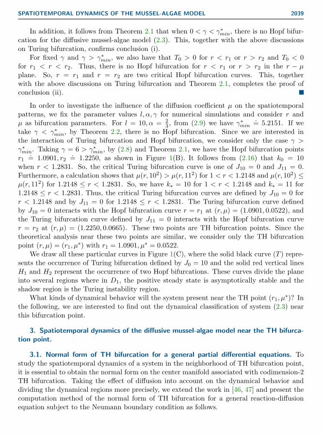
Figure 1. (A): The positive steady state E∗ in (2.4) exists in the regions R1 and R2 but is unstable in R1

and is possible stable in R2 which depends on the choice of γ. (B): Stability/instability regions for the positivesteady state E∗ with α = 2

3 in the r − γ plane. The curve marked by L is the Hopf bifurcation curve. (C):Bifurcation diagram for the diffusive mussel-algae model (2.3) with α = 2

3 , γ = 6 in the r−µ plane. The curvesmarked by H1 and H2 are Hopf bifurcation curves, and the curve marked by T is the Turing bifurcation curve.The shadow region between two curves T and H1 is the Turing instability region.

Theorem 2.2. If the condition (H2) holds, then when 0 < γ < γ∗min, there is no Hopfbifurcation for the diffusive mussel-algae model (2.3).

Proof. From Theorem 2.1 and the definition γ∗min in (2.9), it follows that if the condition(H2) holds and 0 < γ < γ∗min, then T0 > 0. This, together with (2.12), leads to Tk > 0 for anyµ > 0 and k ∈ N0. So, the Hopf bifurcation cannot occur for the diffusive mussel-algae model(2.3) in this case.

Dow

nloa

ded

11/0

3/17

to 2

22.2

04.2

48.1

39. R

edis

trib

utio

n su

bjec

t to

SIA

M li

cens

e or

cop

yrig

ht; s

ee h

ttp://

ww

w.s

iam

.org

/jour

nals

/ojs

a.ph

p



If in the absence of diffusion the positive steady state E∗ is stable under certain conditionbut becomes unstable because of the existence of diffusion, we call this instability the diffusion-driven Turing instability. Thus, diffusion-driven Turing instability occurs only when thereexists at least one positive integer k such that Jk < 0.

Theorem 2.3. If the condition (H2) holds and γ < γ(r, α), then when µ ≥ µ∗, there is nodiffusion-driven Turing instability, where

µ∗ =(r − 1)(1− αr)2

r(1− α)3.

Proof. It is easy from (2.12) to verify that µb22 + 1γ b11 ≤ 0 if and only if µ ≥ µ∗. In

addition, notice that J0 > 0. Thus, if µ ≥ µ∗, then Jk > 0 for any k ∈ N0.

Theorem 2.4. If the condition (H2) holds, then for the diffusive mussel-algae model (2.3),we have the following:

(i) when 0 < γ < γ∗min, the boundary of stability region in the r − µ plane consists of thecritical Turing bifurcation curve µ = µ(r, k2

∗), and there is no TH bifurcation;(ii) when γ > γ∗min, the boundary of stability region in the r − µ plane consists of Hopf

bifurcation curves Hj determined by r = rj , j = 1, 2, and the critical Turing bifurcationcurve µ = µ(r, k2

∗), and TH bifurcation can occur at the interaction points (rj , µ∗) withµ∗ = µ(rj , k2

∗), where µ(rj , k2∗) is determined by (2.13) and k∗ is determined by (2.15)

and (2.16).

Proof. First, we analyze the existence of Turing bifurcation. Solving Jk = 0 determinedby (2.12) for µ, we obtain

µ = µ(r, k2) , A1

k2 −A2

k2 (k2 +A3),(2.13)

where for 0 < α < 1 and 1 < r < 1α ,

A1 =l2(1− αr)α(r − 1)

(1− α)2> 0, A2 = l2(1− α) > 0, A3 =

l2αr(1− α)1− αr

> 0.

It follows from (2.13) that µ(r, k2) > 0 if and only if k > l√

1− α. Further, we have

µ(1, k2) = µ

(1α, k2)

= 0

and

µr(r, k2

)= l2α(k2−A2)

k2(1−α)2(k2+A3)(k2(1−αr)+l2αr(1−α))

(k2(1−αr)(1+α−2αr) + l2α(1−α)

(αr−2αr2+1

))= l2α(k2−A2)

k2(1−α)2(k2+A3)(k2(1−αr)+l2αr(1−α))

(Q1r

2 +Q2r +Q3),

where

Q1 = 2α2 (k2 − l2(1− α)), Q2 = l2α2(1− α)− k2α(3 + α), Q3 = k2(1 + α) + l2α(1− α).

Dow

nloa

ded

11/0

3/17

to 2

22.2

04.2

48.1

39. R

edis

trib

utio

n su

bjec

t to

SIA

M li

cens

e or

cop

yrig

ht; s

ee h

ttp://

ww

w.s

iam

.org

/jour

nals

/ojs

a.ph

p



Noticing that Q1 > 0 for k > l√

1− α, Q3 > 0, and for 1 < r < 1α

µr(1, k2) =

l2α(k2 − l2(1− α))k2(k2 + l2α)

(1− α) > 0, µr

(1α, k2)

=2l2α(k2 −A2)(1− r)k2r(1− α)2(k2 +A3)

< 0,

we have

µr(r, k2){ > 0, 1 < r < r∗,

< 0, r∗ < r < 1α ,

(2.14)

where

r∗ =−Q2 −

√Q2

2 − 4Q1Q3

2Q1

due to µr(r, k2) > 0 for sufficiently large r. It follows from (2.14) that for fixed k, the functionµ = µ(r, k2) is increasing for 1 < r < r∗ and decreasing for r∗ < r < 1

α and obtain itsmaximum at r = r∗.

Assume that z = k2; then µ(r, z) = A1z−A2z(z+A3) . Differentiating µ(r, z) with respect to z

yields

µz(r, z) =−A1

((z −A2)2 −A2

2 −A2A3)

z2(z +A3)2

> 0, 0 < z < z∗,

< 0, z > z∗,

where

z∗ = A2 +√A2 (A2 +A3) = l2 (1− α)

(1 +

1√1− αr

).

The function µ(r, z) reaches its maximum at z = z∗ for z > 0 and fixed r. Therefore, thefunction µ(r, k2) reaches its maximum at k = k∗ for fixed r and k ∈ N = {1, 2, . . .} with

k∗ =

k0, if µ(r, k2

0) ≥ µ(r, (k0 + 1)2

),

k0 + 1, if µ(r, k20) < µ

(r, (k0 + 1)2

),

(2.15)

where

k0 =

[l

√(1− α)

(1 +

1√1− αr

)],(2.16)

where [·] is the integer part function.

Dow

nloa

ded

11/0

3/17

to 2

22.2

04.2

48.1

39. R

edis

trib

utio

n su

bjec

t to

SIA

M li

cens

e or

cop

yrig

ht; s

ee h

ttp://

ww

w.s

iam

.org

/jour

nals

/ojs

a.ph

p



In addition, it follows from Theorem 2.1 that when 0 < γ < γ∗min, there is no Hopf bifur-cation for the diffusive mussel-algae model (2.3). This, together with the above discussionson Turing bifurcation, confirms conclusion (i).

For fixed γ and γ > γ∗min, we also have that T0 > 0 for r < r1 or r > r2 and T0 < 0for r1 < r < r2. Thus, there is no Hopf bifurcation for r < r1 or r > r2 in the r − µplane. So, r = r1 and r = r2 are two critical Hopf bifurcation curves. This, togetherwith the above discussions on Turing bifurcation and Theorem 2.1, completes the proof ofconclusion (ii).

In order to investigate the influence of the diffusion coefficient µ on the spatiotemporalpatterns, we fix the parameter values l, α, γ for numerical simulations and consider r andµ as bifurcation parameters. For l = 10, α = 2

3 , from (2.9) we have γ∗min.= 5.2151. If we

take γ < γ∗min, by Theorem 2.2, there is no Hopf bifurcation. Since we are interested inthe interaction of Turing bifurcation and Hopf bifurcation, we consider only the case γ >γ∗min. Taking γ = 6 > γ∗min, by (2.8) and Theorem 2.1, we have the Hopf bifurcation pointsr1

.= 1.0901, r2.= 1.2250, as shown in Figure 1(B). It follows from (2.16) that k0 = 10

when r < 1.2831. So, the critical Turing bifurcation curve is one of J10 = 0 and J11 = 0.Furthermore, a calculation shows that µ(r, 102) > µ(r, 112) for 1 < r < 1.2148 and µ(r, 102) ≤µ(r, 112) for 1.2148 ≤ r < 1.2831. So, we have k∗ = 10 for 1 < r < 1.2148 and k∗ = 11 for1.2148 ≤ r < 1.2831. Thus, the critical Turing bifurcation curves are defined by J10 = 0 forr < 1.2148 and by J11 = 0 for 1.2148 ≤ r < 1.2831. The Turing bifurcation curve definedby J10 = 0 interacts with the Hopf bifurcation curve r = r1 at (r, µ) = (1.0901, 0.0522), andthe Turing bifurcation curve defined by J11 = 0 interacts with the Hopf bifurcation curver = r2 at (r, µ) = (1.2250, 0.0665). These two points are TH bifurcation points. Since thetheoretical analysis near these two points are similar, we consider only the TH bifurcationpoint (r, µ) = (r1, µ∗) with r1 = 1.0901, µ∗ = 0.0522.

We draw all these particular curves in Figure 1(C), where the solid black curve (T ) repre-sents the occurrence of Turing bifurcation defined by J0 = 10 and the solid red vertical linesH1 and H2 represent the occurrence of two Hopf bifurcations. These curves divide the planeinto several regions where in D1, the positive steady state is asymptotically stable and theshadow region is the Turing instability region.

What kinds of dynamical behavior will the system present near the TH point (r1, µ∗)? Inthe following, we are interested to find out the dynamical classification of system (2.3) nearthis bifurcation point.

3. Spatiotemporal dynamics of the diffusive mussel-algae model near the TH bifurca-tion point.

3.1. Normal form of TH bifurcation for a general partial differential equations. Tostudy the spatiotemporal dynamics of a system in the neighborhood of TH bifurcation point,it is essential to obtain the normal form on the center manifold associated with codimension-2TH bifurcation. Taking the effect of diffusion into account on the dynamical behavior anddividing the dynamical regions more precisely, we extend the work in [46, 47] and present thecomputation method of the normal form of TH bifurcation for a general reaction-diffusionequation subject to the Neumann boundary condition as follows.

Dow

nloa

ded

11/0

3/17

to 2

22.2

04.2

48.1

39. R

edis

trib

utio

n su

bjec

t to

SIA

M li

cens

e or

cop

yrig

ht; s

ee h

ttp://

ww

w.s

iam

.org

/jour

nals

/ojs

a.ph

p



Define the real-valued Sobolev space

X ={u ∈

(W 2,2(0, lπ)

)2,∂ui∂x

= 0, x = 0, lπ, i = 1, 2}

with the inner product

[u, v] =2∑i=1

∫ lπ

0uividx, for u = (u1, u2)T , v = (v1, v2)T ∈ X.

To investigate codimension-2 bifurcation in a system, we introduce two bifurcation pa-rameters, ε1 and ε2, and assume that Turing bifurcation occurs when ε1 = 0, Hopf bifurcationoccurs when ε2 = 0, and consequently TH bifurcation occurs when ε1 = ε2 = 0. To explore theeffect of diffusion coefficient, without loss of generality, we study the general reaction-diffusionsystem

ut = d(ε2)∆u+ L(ε1)u+ F (u, ε1), x ∈ (0, lπ), t > 0,(3.1)

with

u(t) =

(u1(t)u2(t)

), d(ε2)∆ =

((d1 + ε2) ∂2

∂x2 0

0 d2∂2

∂x2

),

L(ε1) = (lij(ε1))2×2 , F (u, ε1) =

(f (1)(u, ε1)

f (2)(u, ε1)

),

and di > 0, i = 1, 2, dom(∆) ⊂ X, ε = (ε1, ε2) ∈ R2, and F : R2 ×R→ R2 are Ck(k ≥ 3) withF (0, ε1) = 0, D1F (0, ε1) = 0.

In the following, we suppose that ε = 0 is the bifurcation value and let L0 = L(0). System(3.1) can be transformed into the following system:

ut = Lu+ F (u, ε)(3.2)

with

Lu =

(d1

∂2

∂x2 0

0 d2∂2

∂x2

)u+ L0u

and

F (u, ε) =

(ε2u1xx

0

)+ L(ε1)u− L0u+ F (u, ε1)

=

(ε2∂2u1∂x2

0

)+

∑j1+j2+j3≥2

1j1!j2!j3!

fj1j2j3uj11 u

j22 ε

j31 , fj1j2j3 =

f(1)j1j2j3

f(2)j1j2j3

.

Dow

nloa

ded

11/0

3/17

to 2

22.2

04.2

48.1

39. R

edis

trib

utio

n su

bjec

t to

SIA

M li

cens

e or

cop

yrig

ht; s

ee h

ttp://

ww

w.s

iam

.org

/jour

nals

/ojs

a.ph

p



The eigenvalues of d∆ are δ(j)k = −dj(kl )2, k ∈ N0, j = 1, 2, and the corresponding normal-

ized eigenfunctions is β(j)k , where

β(j)k (x) = γk(x)ej , γk(x) =

cos(kxl

)‖cos

(kxl

)‖2,2

=

1√lπ, for k = 0,√

2lπ cos

(kxl

), for k 6= 0,

(3.3)

where ej is the unit coordinate vector of R2 and k is usually called wave number.The characteristic equation associated with the linearized system of (3.2) is

∏k∈N0

Γk(λ) =

0, where Γk(λ) = det(Mk(λ)) with Mk(λ) = diag{λ − δ(1)k , λ − δ(2)

k } − L0. Assume that theequation Γ0(λ) = 0 has a pair of simple purely imaginary roots ±iω and there exists an integerk∗ ∈ N such that the equation Γk∗(λ) = 0 has a simple zero root λ = 0. Moreover, all theother roots of

∏k∈N0

Γk(λ) = 0 have negative real parts.For two vectors ϕ,ψ ∈ R2, denote their scalar product 〈ψT , ϕ〉 = ψTϕ. Let

Φ0 = (p0, p0),Φk∗ = pk∗ ,Ψ0 = col(qT0 , q0

T),Ψk∗ = qTk∗ ,

where p0 = (p01, p02)T ∈ C2 and pk∗ = (pk∗1, pk∗2)T ∈ R2 are the eigenvectors associated withthe eigenvalues iω and 0, respectively; q0 = (q01, q02)T ∈ C2 and qk∗ = (qk∗1, qk∗2)T ∈ R2 arethe corresponding adjoint eigenvectors; and 〈Ψ0,Φ0〉 = I2, 〈Ψk∗ ,Φk∗〉 = 1. Then u ∈ C can bedecomposed as

u =

(Φ0

(z1

z2

))T (β

(1)0

β(2)0

)+ (Φk∗z3)

(β

(1)k∗

β(2)k∗

)+ w

= (z1p0 + z2p0)γ0(x) + z3pk∗γk∗(x) +

(w1

w2

),(3.4)

where z1, z2, z3 ∈ R, w ∈ Xs.Let Φ=diag{Φ0,Φk∗} and zx=(z1γ0, z2γ0, z3γk∗)

T . Then u = Φzx+w. B=diag{iω,−iω, 0}is a diagonal matrix, the operator M1

j , j ≥ 2 defined in V 5j (R3), and we have a diagonal

representation relative to the canonical basis {zq11 zq22 z

q33 ε

p11 ε

p22 ek, q1, q2, q3, p1, p2 ∈ N0, q1 +

q2 + q3 + p1 + p2 = j}, where ek(k = 1, 2, 3) are unit vectors. It is easy to verify that

M1j (εpzqeς)Bz −Bεpzqeς = iω (q1 − q2 + (−1)ς) εpzqeς ,

M1j (εpzqe3)Bz −Bεpzqe3 = iω (q1 − q2) εpzqe3,(3.5)

where ς = 1, 2. Then, from (3.5), we get

Ker(M1

2)

= span{z1z3e1, z1ε1e1, z1ε2e1, z2z3e2, z2ε1e2, z2ε2e2, z1z2e3, z

23e3, z3ε1e3, z3ε2e3,

ε1ε2e3, ε21e3, ε

22e3}

(3.6)

and

Ker(M1

3)

= span{z21z2e1, z1z

23e1, z1z3ε1e1, z1z3ε2e1, z1ε

21e1, z1ε

22e1, z1ε1ε2e1, z1z

22e2, z2z

23e2,

z2z3ε1e2, z2z3ε2e2, z2ε21e2, z2ε

22e2, z2ε1ε2e2, z1z2z3e3, z

33e3, z1z2ε1e3,

z1z2ε2e3, z3ε21e3, z3ε

22e3, z3ε1ε2e3

}.(3.7)D

ownl

oade

d 11

/03/

17 to

222

.204

.248

.139

. Red

istr

ibut

ion

subj

ect t

o SI

AM

lice

nse

or c

opyr

ight

; see

http

://w

ww

.sia

m.o

rg/jo

urna

ls/o

jsa.

php



Following the results in [46, 47], we have the normal form for TH bifurcation as follows:

z = Bz +

(B

(1)1 ε1 +B

(2)1 ε2

)z1(

B(1)2 ε1 +B

(2)2 ε2

)z2(

B(1)3 ε1 +B

(2)3 ε2

)z3

+

B11z21z2 +B12z1z

23

B21z1z22 +B22z2z

23

B31z1z2z3 +B32z33

+

B13z1ε21 +B14z1ε

22 +B15z1ε1ε2

B23z2ε21 +B24z2ε

22 +B25z2ε1ε2

B33z3ε21 +B34z3ε

22 +B35z3ε1ε2

+ h.o.t.,(3.8)

where

B1j = C1j +32

(D1j + E1j) = B2j , B3j = C3j +32

(D3j + E3j), j = 1, 2, 3, 4, 5,

with the expression of B1j , B2j , B3j , j = 1, 2 being the same as in [47] (see Appendix A). In thispaper, we focus on finding the expression of B(1)

i , B(2)i , i = 1, 2, 3 and B1j , B2j , B3j , j = 3, 4, 5

(see Appendix B).As for autonomous ODEs in the finite dimension space, by a recursive transformation of

variables

(z, w) = (z, w) +1j!(U1j (z, ε), U2

j (z, ε)), j ≥ 2,

where U1j and U2

j are homogeneous polynomials of degree j in z and ε. The normal form onthe center manifold becomes

z = Bz +12!g12(z, 0, ε) +

13!g13(z, 0, ε) +O

(|ε||z|2

),(3.9)

where g12 and g1

3 are the second and third terms in (z, ε), respectively, by dropping the tildeafter each transformation of variable for simplification of notation.

The normal form (3.8) can be written in real coordinates ω through the change of variablesz1 = v1 − v2i, z2 = v1 + v2i, z3 = v3, and then in cylindrical coordinates by v1 = ρ cos Θ, v2 =ρ sin Θ, v3 = s. Truncating at third-order terms and removing the azimuthal term, finally,(3.8) is equivalent to the following:{

ρ = ν1(ε)ρ+ κ11ρ3 + κ12ρs

2,

s = ν2(ε)s+ κ21ρ2s+ κ22s

3,(3.10)

where

ν1(ε) = Re(B

(1)1 ε1 +B

(2)1 ε2 +B13ε

21 +B14ε

22 +B15ε1ε2

),

ν2(ε) = Re(B

(1)3 ε1 +B

(2)3 ε2 +B33ε

21 +B34ε

22 +B35ε1ε2

),

κ11 = Re (B11) , κ12 = Re (B12) , κ21 = Re (B31) , κ22 = Re (B32) .

Dow

nloa

ded

11/0

3/17

to 2

22.2

04.2

48.1

39. R

edis

trib

utio

n su

bjec

t to

SIA

M li

cens

e or

cop

yrig

ht; s

ee h

ttp://

ww

w.s

iam

.org

/jour

nals

/ojs

a.ph

p



3.2. Dynamical classification of the diffusive mussel-algae model near the TH bifur-cation point. In this subsection, we apply the theoretical results developed previously to thediffusive mussel-algae model to obtain the normal form of TH bifurcation; then we can classifythe dynamics near the TH bifurcation point explicitly.

From Theorem 2.4 (ii) and Figure 1(C), when α = 2/3, γ = 6, the point TH(r1, µ∗) withr1 = 1.0901, µ∗ = 0.0522 in the r − µ plane is the TH bifurcation point of system (2.3). Toapply the results in section 3.1, we set ε1 = r − r1, ε2 = µ− µ∗ , l = 10, k∗ = 10, and rewritethe positive steady state as a parameter-dependent form E∗(m∗(ε1), a∗(ε1)) with

m∗ (ε1) =α (r1 + ε1 − 1)1− α (r1 + ε1)

, a∗ (ε1) =1− α (r1 + ε1)

(r1 + ε1) (1− α).

Setting m(x, t) = m(x, t) −m∗(ε1), a(x, t) = a(x, t) − a∗(ε1), u(x, t) = (m(x, t), a(x, t))T andthen dropping the tides for simplification of notation, the system (2.3) can be written as(3.2) with

u=

(m(x, t)a(x, t)

), Lu=

(µ∗mxx

1γaxx

)+L0u, F (u, ε)=

(ε2mxx

0

)+F (u, ε1),

where

L(ε1) =

(b11 (ε1) b12 (ε1)b21 (ε1) b22 (ε1)

), L0 = L(0), F (u, ε1) =

(f (1)(u, ε1)

f (2)(u, ε1)

),

and bij(ε1) is defined by (2.6) with r = r1 + ε1,

f (1) (m, a, ε1) = (r1 + ε1) (m+m∗(ε1)) (a+ a∗ (ε1))− m+m∗ (ε1)1 +m+m∗(ε1)

,

f (2) (m, a, ε1) =α

γ(1− (a+ a∗ (ε1)))− 1

γ(m+m∗ (ε1)) (a+ a∗(ε1)) .

Let

Mk =

(−µ∗ k2

l2+ b11 (0) b12 (0)

b21 (0) − 1γk2

l2+ b22 (0)

).

It is easy to verify that Φ0 = (p0, p0),Φk∗ = pk∗ ,Ψ0 = (q0, q0)T ,Ψk∗ = qk∗ , where

p0 =

(p01

p02

)=

1(iω0(1−α)2−(1−αr1)α(r1−1))(1−αr1)

αr1(r1−1)(1−α)2

,

qT0 =(q01, q02

)=(

iω0γ(1−αr1)+αr1(1−α)2iω0γ(1−αr1) , αr1(r1−1)

2iω0(1−αr1)

),

pk∗ =

(pk∗1

pk∗2

)=

1(µ∗ k∗2

l2(1−α)2−(1−αr1)α(r1−1)

)(1−αr1)

αr1(r1−1)(1−α)2

,

qTk∗ =(qk∗1, qk∗2

)=(

k∗2l2

+αr1(1−α)γ(1−αr1)Tk∗

, αr1(r1−1)(1−αr1)Tk∗

),

with ω0 =√

1γα(r1−1)(1−αr1)

1−α .

Dow

nloa

ded

11/0

3/17

to 2

22.2

04.2

48.1

39. R

edis

trib

utio

n su

bjec

t to

SIA

M li

cens

e or

cop

yrig

ht; s

ee h

ttp://

ww

w.s

iam

.org

/jour

nals

/ojs

a.ph

p



By a direct computation, we obtain f020 = f210 = f120 = f030 = 0. Then, according to theprocedure in section 3.1, the normal form truncated to the third-order terms is

ρ =(0.3917ε1 − 2.6035ε21

)ρ− 0.0125624ρ3 + 0.0045ρs2,

s =(0.5309ε1 − 1.4364ε2 − 1.7079ε21 − 2.8640ε22 − 2.8627ε1ε2

)s

− 0.0236ρ2s− 0.0340s3.

(3.11)

Notice that ρ ≥ 0 and s is arbitrarily real number. System (3.11) has a zero equilibriumA0(0, 0) for all ε1, ε2, three possible boundary equilibria

A1

(√0.3917ε1 − 2.6035ε21

0.0125, 0

),

A±2

(0,±

√0.5309ε1 − 1.4364ε2 − 1.7079ε21 − 2.8640ε22 − 2.8627ε1ε2

0.0340

),

and two possible positive equilibria A±3 (ρ∗,±s∗), where

ρ∗ =

√0.1571ε1 − 0.0646ε2 − 0.9621ε21 − 0.1289ε22 − 0.1288ε1ε2

0.0054

and

s∗ =

√−(0.0260ε1 + 0.1795ε2 − 0.4009ε21 + 0.3580ε22 + 0.3578ε1ε2)

0.0054.

From the existence and their stability of these five equilibria, we obtain the critical bifurcationlines as follows:

H : ε1 = 0;

T : 0.5309ε1 − 1.4364ε2 − 1.7079ε21 − 2.8640ε22 − 2.8627ε1ε2 = 0;

T1 : 0.1571ε1 − 0.0646ε2 − 0.9621ε21 − 0.1289ε22 − 0.1288ε1ε2 = 0, ε1 < 0;

T2 : 0.0260ε1 + 0.1795ε2 − 0.4009ε21 + 0.3580ε22 + 0.3578ε1ε2 = 0, ε1 > 0.

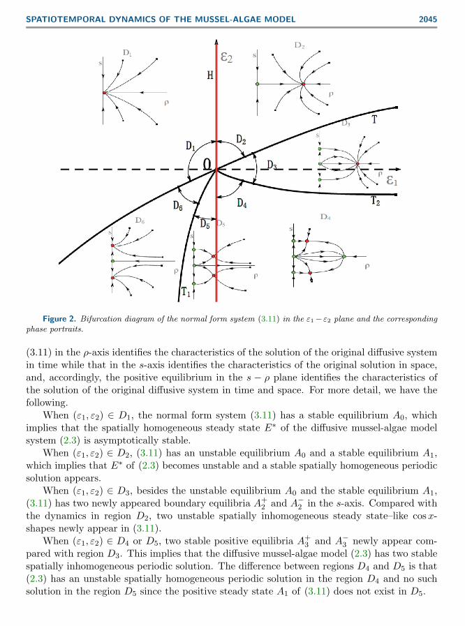
Notice that the normal form (3.11) belongs to the so-called simple case described in [15].Therefore, the bifurcation diagrams in the (ε1, ε2) parameter space and the correspondingphase portraits of the normal form system (3.11) plane can be shown in Figure 2. These foursolid lines H,T, T1, and T2 divide the (ε1, ε2) parameter plane into six regions with differentdynamics.

According to the normal form theory of reaction-diffusion equations [9, 47], the dynamicsof the normal form system (3.11) is topologically equivalent to the dynamics of the originaldiffusive system near the bifurcation point. In addition, notice that ε1 and ε2 are perturba-tion variables, respectively, of the original parameters r and µ in the diffusive mussel-algaemodel system (2.3) at r = r1, µ = µ∗. Thus, the dynamical classification of (2.3) nearthe TH bifurcation point TH(r1, µ∗) can be determined by the normal form system (3.11).By the procedure of the calculation of the normal form, it is easy to see that the equilibrium of

Dow

nloa

ded

11/0

3/17

to 2

22.2

04.2

48.1

39. R

edis

trib

utio

n su

bjec

t to

SIA

M li

cens

e or

cop

yrig

ht; s

ee h

ttp://

ww

w.s

iam

.org

/jour

nals

/ojs

a.ph

p



Figure 2. Bifurcation diagram of the normal form system (3.11) in the ε1−ε2 plane and the correspondingphase portraits.

(3.11) in the ρ-axis identifies the characteristics of the solution of the original diffusive systemin time while that in the s-axis identifies the characteristics of the original solution in space,and, accordingly, the positive equilibrium in the s − ρ plane identifies the characteristics ofthe solution of the original diffusive system in time and space. For more detail, we have thefollowing.

When (ε1, ε2) ∈ D1, the normal form system (3.11) has a stable equilibrium A0, whichimplies that the spatially homogeneous steady state E∗ of the diffusive mussel-algae modelsystem (2.3) is asymptotically stable.

When (ε1, ε2) ∈ D2, (3.11) has an unstable equilibrium A0 and a stable equilibrium A1,which implies that E∗ of (2.3) becomes unstable and a stable spatially homogeneous periodicsolution appears.

When (ε1, ε2) ∈ D3, besides the unstable equilibrium A0 and the stable equilibrium A1,(3.11) has two newly appeared boundary equilibria A+

2 and A−2 in the s-axis. Compared withthe dynamics in region D2, two unstable spatially inhomogeneous steady state–like cosx-shapes newly appear in (3.11).

When (ε1, ε2) ∈ D4 or D5, two stable positive equilibria A+3 and A−3 newly appear com-

pared with region D3. This implies that the diffusive mussel-algae model (2.3) has two stablespatially inhomogeneous periodic solution. The difference between regions D4 and D5 is that(2.3) has an unstable spatially homogeneous periodic solution in the region D4 and no suchsolution in the region D5 since the positive steady state A1 of (3.11) does not exist in D5.D

ownl

oade

d 11

/03/

17 to

222

.204

.248

.139

. Red

istr

ibut

ion

subj

ect t

o SI

AM

lice

nse

or c

opyr

ight

; see

http

://w

ww

.sia

m.o

rg/jo

urna

ls/o

jsa.

php



When (ε1, ε2) ∈ D6, (3.11) has only one unstable zero equilibrium and two stable boundaryequilibria A+

2 and A−2 in the s-axis. This implies that the diffusive mussel-algae model (2.3)has three steady states: one is unstable and spatially homogeneous, and the other two arestable and spatially inhomogeneous.

We should address that the theory and method developed in this section is targeted atthe dynamical behavior near a TH bifurcation point by obtaining the normal forms throughthe coordinate transformations and analyzing the dynamical information from the truncatednormal forms. Once the conditions are determined for occurring TH bifurcation at the steadystate, this method is valid, although only the local dynamical properties can be investigated.

3.3. Numerical simulations.

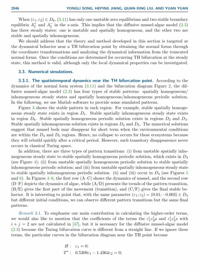
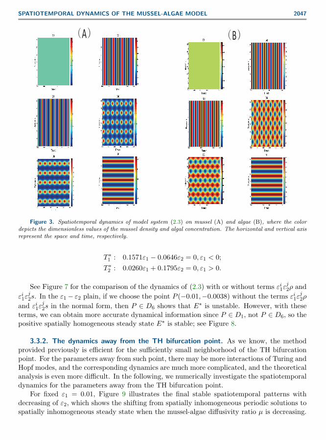
3.3.1. The spatiotemporal dynamics near the TH bifurcation point. According to thedynamics of the normal form system (3.11) and the bifurcation diagram Figure 2, the dif-fusive mussel-algae model (2.3) has four types of stable patterns: spatially homogeneous/inhomogeneous steady states and spatially homogeneous/inhomogeneous periodic solution.In the following, we use Matlab software to provide some simulated patterns.

Figure 3 shows the stable pattern in each region. For example, stable spatially homoge-neous steady state exists in region D1. Stable spatially inhomogeneous steady state existsin region D6. Stable spatially homogeneous periodic solution exists in regions D2 and D3.Stable spatially inhomogeneous solution exists in regions D4 and D5. The numerical solutionssuggest that mussel beds may disappear for short term when the environmental conditionsare within the D4 and D5 regions. Hence, no collapse to occurs for these ecosystems becausethey will rebuild quickly after a critical period. However, such transitory disappearence neveroccurs in classical Turing space.

In addition, there are three types of pattern transitions: (i) from unstable spatially inho-mogeneous steady state to stable spatially homogeneous periodic solution, which exists in D3(see Figure 4); (ii) from unstable spatially homogeneous periodic solution to stable spatiallyinhomogeneous periodic solution; and (iii) from unstable spatially inhomogeneous steady stateto stable spatially inhomogeneous periodic solution. (ii) and (iii) occur in D4 (see Figures 5and 6). In Figures 4–6, the first row (A–C) shows the dynamics of mussel, and the second row(D–F) depicts the dynamics of algae, while (A/D) presents the trends of the pattern transition,(B/E) gives the first part of the movement (transition), and (C/F) gives the final stable be-havior. It is interesting to point that, with the same parameter (ε1; ε2) = (0.01;−0.003) ∈ D4but different initial conditions, we can observe different pattern transitions but the same finalpatterns.

Remark 3.1. To emphasize our main contribution in calculating the higher-order terms,we would also like to mention that the coefficients of the terms the εi1ε

j2ρ and εi1ε

j2s with

i + j = 2 are not calculated in [47], but it is necessary for the diffusive mussel-algae model(2.3) because the Turing bifurcation curve is different from a straight line. If we ignore theseterms, the particular curves in the bifurcation diagram near the TH point become

H : ε1 = 0;T ∗ : 0.5309ε1 − 1.4364ε2 = 0;

Dow

nloa

ded

11/0

3/17

to 2

22.2

04.2

48.1

39. R

edis

trib

utio

n su

bjec

t to

SIA

M li

cens

e or

cop

yrig

ht; s

ee h

ttp://

ww

w.s

iam

.org

/jour

nals

/ojs

a.ph

p



Figure 3. Spatiotemporal dynamics of model system (2.3) on mussel (A) and algae (B), where the colordepicts the dimensionless values of the mussel density and algal concentration. The horizontal and vertical axisrepresent the space and time, respectively.

T ∗1 : 0.1571ε1 − 0.0646ε2 = 0, ε1 < 0;T ∗2 : 0.0260ε1 + 0.1795ε2 = 0, ε1 > 0.

See Figure 7 for the comparison of the dynamics of (2.3) with or without terms εi1εj2ρ and

εi1εj2s. In the ε1− ε2 plain, if we choose the point P (−0.01,−0.0038) without the terms εi1ε

j2ρ

and εi1εj2s in the normal form, then P ∈ D6 shows that E∗ is unstable. However, with these

terms, we can obtain more accurate dynamical information since P ∈ D1, not P ∈ D6, so thepositive spatially homogeneous steady state E∗ is stable; see Figure 8.

3.3.2. The dynamics away from the TH bifurcation point. As we know, the methodprovided previously is efficient for the sufficiently small neighborhood of the TH bifurcationpoint. For the parameters away from such point, there may be more interactions of Turing andHopf modes, and the corresponding dynamics are much more complicated, and the theoreticalanalysis is even more difficult. In the following, we numerically investigate the spatiotemporaldynamics for the parameters away from the TH bifurcation point.

For fixed ε1 = 0.01, Figure 9 illustrates the final stable spatiotemporal patterns withdecreasing of ε2, which shows the shifting from spatially inhomogeneous periodic solutions tospatially inhomogeneous steady state when the mussel-algae diffusivity ratio µ is decreasing.

Dow

nloa

ded

11/0

3/17

to 2

22.2

04.2

48.1

39. R

edis

trib

utio

n su

bjec

t to

SIA

M li

cens

e or

cop

yrig

ht; s

ee h

ttp://

ww

w.s

iam

.org

/jour

nals

/ojs

a.ph

p



Figure 4. When (ε1, ε2) = (0.02, 0.001) ∈ D3 and the initial values are (m0, a0) = (0.2824 −0.05 cosx, 0.7025 + 0.03 cosx), the positive constant steady state E∗ of system (2.3) is unstable. (A)–(C):The dynamics of mussel; (D)–(F): The dynamics of algae. There are unstable spatially inhomogeneous steadystates and stable homogeneous periodic solutions, so there exists an orbit connecting these two states.

Figure 5. When (ε1, ε2) = (0.01,−0.003) ∈ D4 and the initial values are (m0, a0) = (0.15 − 0.005 cosx,0.5− 0.005 cosx), the positive constant steady state E∗ of system (2.3) is unstable. (A)–(C): The dynamics ofmussel; (D)–(F): The dynamics of algae. There are unstable spatially homogeneous periodic solution and stablespatially inhomogeneous periodic solutions, so there exists an orbit connecting these two states.

Dow

nloa

ded

11/0

3/17

to 2

22.2

04.2

48.1

39. R

edis

trib

utio

n su

bjec

t to

SIA

M li

cens

e or

cop

yrig

ht; s

ee h

ttp://

ww

w.s

iam

.org

/jour

nals

/ojs

a.ph

p



Figure 6. When (ε1, ε2) = (0.01,−0.003) ∈ D4 and the initial values are (m0, a0) = (0.2503 −0.06 cosx, 0.7270 + 0.02 cosx), the positive constant steady state E∗ of system (2.3) is unstable. (A)–(C):The dynamics of mussel; (D)–(F): The dynamics of algae. There are unstable spatially inhomogeneous steadystates and stable spatially inhomogeneous periodic solutions, so there exists an orbit connecting these two states.

Figure 7. Comparison of bifurcation diagram of the normal form system (3.11) with (solid curves) orwithout (dashed lines) the terms εi

1εj2ρ and εi

1εj2s with i+ j = 2.

Dow

nloa

ded

11/0

3/17

to 2

22.2

04.2

48.1

39. R

edis

trib

utio

n su

bjec

t to

SIA

M li

cens

e or

cop

yrig

ht; s

ee h

ttp://

ww

w.s

iam

.org

/jour

nals

/ojs

a.ph

p



Figure 8. When (ε1, ε2) = (−0.01,−0.0038) and the initial values are (m0, a0) = (0.15− 0.005 cosx, 0.6−0.005 cosx), the positive constant steady state E∗ of system (2.3) is asymptotically stable.

Figure 9. For fixed ε1 = 0.01, the dynamics is changed with the decreasing of ε2. (A) and (D): ε2 = −0.013and spatially inhomogeneous periodic solutions; (B) and (E): ε2 = −0.015 and spatially inhomogeneous steadystate with wide strips; (C) and (F): ε2 = −0.052 and spatially inhomogeneous steady state with narrow strips.(A)–(C): The dynamics of mussel; (D)–(F): The dynamics of algae.

Comparing with Figure 6(C,F), where ε2 = −0.003, we can see that when ε2 = −0.013, thespatially inhomogeneous periodic solution remains, and it disappears as ε2 ≤ −0.015 with theoccurrence of the spatially inhomogeneous steady state with strips.

3.3.3. The influence of the advection on the dynamics. To the best of our knowledge,in the literature there is no theoretical work done yet about the normal form computationin the model with the advection term, which is not trivial. Here we discuss the influence ofadvection on the system (2.2) by using the numerical method. Comparing with Figure 3, wherethere is no advection involved in the system, we can observe the motion change due to theintroduction of the advection, such as the loss of the stability of the steady state and the break

Dow

nloa

ded

11/0

3/17

to 2

22.2

04.2

48.1

39. R

edis

trib

utio

n su

bjec

t to

SIA

M li

cens

e or

cop

yrig

ht; s

ee h

ttp://

ww

w.s

iam

.org

/jour

nals

/ojs

a.ph

p



Figure 10. When (ε1, ε2) = (−0.01, 0.001) ∈ D1, the dynamics is changed with the increasing of the valueof advection ν. ν = 0.4 for (A) and (D), ν = 0.42 for (B) and (E), and ν = 0.8 for (C) and (F). (A)–(C): Thedynamics of mussel; (D)–(F): The dynamics of algae.

of the spatially homogeneous oscillations. For instance, when (ε1, ε2) = (−0.01, 0.001) ∈ D1,the steady state of (2.3) is stable (see Figure 3(A(D1),B(D1))). Such stability stays forsmall advection and loses the stability when the advection value reaches a critical value (seeFigure 10). When (ε1, ε2) = (0.02, 0.001) ∈ D2 or (ε1, ε2) = (0.01,−0.003) ∈ D4, by thecomparison of the figures, i.e., Figure 11 vs. Figure 3 (A(D2),B(D2)) and Figure 12 vs.Figure 3(A(D4),B(D4)), respectively, we can view the connecting dynamics showing the lossof stable spatially homogeneous steady state or oscillation.

4. Discussion and conclusion. In this paper, we have derived the normal form compu-tation for a general reaction-diffusion equation by taking the effect of diffusion into account,then applying the results to study TH bifurcation for the diffusive mussel-algae model underthe homogeneous Neumann boundary condition.

The stability and Hopf bifurcation of the positive equilibrium of the corresponding ODEsystem (2.4) is determined according to the parameters r (a measure of the growth rate ofmussel) and γ (a parameter indicates the mortality of mussels). When γ is less than thecritical value γ∗min, the positive equilibrium is always stable independent of r. However, whenγ is larger than γ∗min, r plays an important role in determining the stability of the positiveequilibrium and the existence of Hopf bifurcation, and it can lead to periodic oscillation.

For the diffusive mussel-algae model, we discuss the mussel-algae diffusivity ratio µ andthe growth rate r of mussel on the stability and TH bifurcation of the positive steady stateof systems (2.3). More precisely, if we fixed γ less than γ∗min, there is no TH bifurcation, andonly diffusion-driven Turing instability occurs. When γ is sufficiently small, the authors haveinvestigated in detail the Turing patterns for two-dimensional spatial variables and found

Dow

nloa

ded

11/0

3/17

to 2

22.2

04.2

48.1

39. R

edis

trib

utio

n su

bjec

t to

SIA

M li

cens

e or

cop

yrig

ht; s

ee h

ttp://

ww

w.s

iam

.org

/jour

nals

/ojs

a.ph

p



Figure 11. When (ε1, ε2) = (0.02, 0.001) ∈ D2, the dynamics is changed with the increasing of the value ofadvection ν. ν = 0.38 for (A) and (D), ν = 0.46 for (B) and (E), and ν = 0.8 for (C) and (F). (A)–(C): Thedynamics of mussel; (D)–(F): The dynamics of algae.

Figure 12. When (ε1, ε2) = (0.01,−0.003) ∈ D4, the dynamics is changed with the increasing of the valueof advection ν. ν = 0.2 for (A) and (D), ν = 0.4 for (B) and (E), and ν = 0.8 for (C) and (F). (A)–(C): Thedynamics of mussel; (D)–(F): The dynamics of algae.

Dow

nloa

ded

11/0

3/17

to 2

22.2

04.2

48.1

39. R

edis

trib

utio

n su

bjec

t to

SIA

M li

cens

e or

cop

yrig

ht; s

ee h

ttp://

ww

w.s

iam

.org

/jour

nals

/ojs

a.ph

p



different patterns, such as rhombic or hexagonal arrays and isolated clusters of clumps orgaps, an intermediate labyrinthine state by employing weakly nonlinear diffusive instabilityanalyses in [3]. However, we show that the critical value γ∗min is analytically determined.

If we fixed γ larger than γ∗min , which is not considered in [3], the stability, Turing insta-bility, and TH bifurcation of the positive steady state of system (2.3) is investigated accordingto the potential growth rate r of mussel and the mussel-algae diffusivity ratio µ. When µis fixed and larger than the critical value, the system (2.3) first undergoes Hopf bifurcationand then Turing bifurcation as r is increasing, while when µ is fixed and smaller than thecritical value, the story is reverse; i.e., the system (2.3) first undergoes Turing bifurcation andthen Hopf bifurcation. Furthermore, the spatiotemporal dynamical classification near the THbifurcation point is investigated in detail by using normal form theory. The parameter re-gions for occurrence of stable spatial homogeneous/homogeneous periodic solutions and stablehomogeneous/homogeneous steady states are explicitly determined. We also found three typesof pattern transitions, which are also called oscillatory Turing patterns and previously foundusing numerical method in [62, 63]. Stable spatial homogeneous periodic solutions make upanother new foundation, which is the result of interaction of Turing bifurcation and Hopfbifurcation and cannot occur for only Hopf bifurcation or Turing bifurcation.

From numerical simulations, it is easy to observe that the diffusion µ and the growthrate r of mussel could result in complex dynamics of system (2.3). It is well known that theresulting spatial complexity is characteristic of many natural ecosystems. The mussel bedsare spatial homogeneously distribution and spatial inhomogeneously distribution by varyingthe diffusion µ of mussel, which imply that the diffusive instabilities might explain instancesof spatial irregularities for natural communities. The growth rate r of mussel also reflectsthe interaction relationship between mussel and algae. So, the spatial distribution of algae iseffected by the quantitative changes of mussel.

A very conspicuous features of patterned mussel beds is that they can develop from twodifferent paths caused by the TH bifurcation (see Figures 5 and 6). These patterns display acoherent spatiotemporal oscillation behavior. Recently, it is reported in [20] that the patternformation displays contrary ecosystem functioning arising from different ecological processesin spite of similar spatial patterns emergence. Hence, it is interesting to further explore thepatterns stability and their ecological functions underlying the TH bifurcation in future work.One of the most relative functions is to clarify their differences of the ecological resiliencefollowing disturbance near the TH bifurcation. In the model of van de Koppel et al. [50] forpattern formation in mussel beds, a constant inshore advection of algae for the tidal flow isassumed. There are two aspects that should be extended and further improved in this model.First, in reality, the direction of advection oscillates with the tide. This periodic oscillationremarkably affects the development of spatial patterns on mussel beds [42]. Going beyond thisadvection, algal cells always disperse with Brownian motion in the water [8]. Particularly, thisrandom Brownian movement behavior dominates the algae behavior in the boundary layer.Toward our objective to investigate the way in which these dispersion processes affect thepotential for pattern formation, we have shown the four different spatial patterns underlyingthe assumption of dispersion processes, which were not identified in previous studies [3] ofthis models. Understanding the dynamics of mussel beds is an important topic due to its

Dow

nloa

ded

11/0

3/17

to 2

22.2

04.2

48.1

39. R

edis

trib

utio

n su

bjec

t to

SIA

M li

cens

e or

cop

yrig

ht; s

ee h

ttp://

ww

w.s

iam

.org

/jour

nals

/ojs

a.ph

p



economical benefit in many parts of the world. Predicting their spatiotemporal behaviors isan important step for restoration programs and mussel fisheries.

In ecosystems, one of the most intriguing functions of the spatial patterning is acting asthe indicator for impending regime shift [31, 40] and ecological degradations [13]. Currently,such a significant ecological role is understood only by the pure Turing instability scenarioswith linear stability predictions [6, 20]. There is a lack of a full comprehension of the spatialnonlinear dynamical behaviors, such as local patterns and hysteresis phenomena, in manyecosystems [39, 41, 42]. Our bifurcation analysis reveals that the indicator function maydisappear when the relevant parameters lie in the TH bifurcation region, for example, inFigure 3(D2,D5), where the alternative emergencies of spatial patterns (or biomass) ascribe thetime-series oscillations rather than the environmental degradation. Hence, analyzing the THinteractions could help us understand the ecosystems functioning—resilience and catastrophicshift—on spatial self-organization patterning.

In modeling the mussel bed ecosystems, the advection term is usually used to depict thetidal fluid direction where the water come from the sea to coast, and the diffusion term depictsthe isotropic dispersion on horizontal planes. Although they are involved in two differentecological processes, advection and diffusion terms have the same mechanism—an active-inhibitor principle [21]. For the emergent properties of spatial self-organization patterns,the advection and diffusion are equivalent. With both advection and diffusion in the algalequation based on the van de Koppel model, one could use a dimensionless peclet number—aratio related to these two processes to describe the influence of the joint effects that is beyondthe scope of this paper. It is shown in [42, 52] that the qualitative properties are similar,although there is a slight difference in the quantitative prediction of onset of spatial patterns.How do we predict the dynamical behavior theoretically for the system with both advectionand diffusion terms explicitly? We leave this as a potential topic for future research.

Appendix A. Calculation of the B1j, B2j, B3j, j = 1, 2.

B11 = C11 +32

(D11 + E11) = B21, B31 = C31 +32

(D31 + E31) ,

B12 = C12 +32

(D12 + E12) = B2j , B32 = C32 +32

(D32 + E32) ,

where

C11 =1

2lπqT0 A210 = C21, C12 =

12lπ

qT0 A102 = C22, C31 =1lπqTk∗A111, C32 =

14lπ

qTk∗A003,

and

D11 =1

3liπω0

[−(qT0 A200

) (qT0 A110

)+

13(qT0 A020

) (qT0 A200

)+ 2

(qT0 A110

)2]= D21,

D12 =1

3liπω0

[−(qT0 A200

) (qT0 A002

)+(qT0 A110

) (q0TA002

)+ 2

(qT0 A002

) (qT0 A101

)]= D22,

D31 = − 13lπω0

Im{(qT0 A110

) (qTk∗A101

)}, D32 = − 2

3lπω0Im{(qT0 A002

) (qTk∗A101

)},

Dow

nloa

ded

11/0

3/17

to 2

22.2

04.2

48.1

39. R

edis

trib

utio

n su

bjec

t to

SIA

M li

cens

e or

cop

yrig

ht; s

ee h

ttp://

ww

w.s

iam

.org

/jour

nals

/ojs

a.ph

p



and

E11 =1

3√lπqT0[H2(0, p0, h0110) +H2(0, p0, h0200)

]= E21,

E12 =1

3√lπqT0 [H2(0, p0, h0002) +H2(0, pk∗ , hk∗101)] = E22,

E31 =1

3√lπqTk∗[H2(0, p0, hk∗011) +H2(0, p0, hk∗101)

+ H2(0, pk∗ , h0110)] +1

3√

2lπqTk∗H2

(0, pk∗ , h(2k∗)110

),

E32 =1

3√lπqTk∗H2(0, pk∗ , h0002) +

13√

2lπqTk∗H2

(0, pk∗ , h(2k∗)002

),

with

h0200 =1√lπ

(2iω0I −M0)−1 (A200 − qT0 A200p0 − q0TA200p0),

h0020 =1√lπ

(−2iω0I −M0)−1 (A020 − qT0 A020p0 − q0TA020p0),

h0002 = − 1√lπM−1

0(A002 − qT0 A002p0 − q0TA002p0

),

h0110 = − 2√lπM−1

0(A110 − qT0 A110p0 − q0TA110p0

),

hk∗101 =2√lπ

(iω0I −Mk∗)−1 (A101 − qTk∗A101pk∗

),

hk∗011 =2√lπ

(−iω0I −Mk∗)−1 (A011 − qTk∗A011pk∗

),

h(2k∗)002 = − 1√2lπM−1

2k∗A002, h(2k∗)110 = (0, 0)T .

Appendix B. Calculation of B(1)i , B

(2)i , i = 1, 2, 3, and B1j, B2j, B3j, j = 3, 4, 5.

By the previous results of [46, 47] and (3.4), we obtain f12 (z, 0, ε) as follows:

f12 (z, 0, ε) = Ψ(0)

[

2

((ε2

∂2

∂x2

0

)+ L1 (ε1)

)(Φzx) + F2 (Φzx, ε1) , β(1)

ν

][

2

((ε2

∂2

∂x2

0

)+ L1 (ε1)

)(Φzx) + F2 (Φzx, ε1) , β(2)

ν

]ν=k∗

ν=0

,

(B.1)

where Ψ(0) = diag{Ψ0,Ψk∗}, and((ε2

∂2

∂x2

0

)+ L1(ε1)

)(Φzx)

= P10010z1ε1γ0(x) + P01010z2ε1γ0(x) + P00110z3ε1γk∗(x) + P00101z3ε2γk∗(x),

Dow

nloa

ded

11/0

3/17

to 2

22.2

04.2

48.1

39. R

edis

trib

utio

n su

bjec

t to

SIA

M li

cens

e or

cop

yrig

ht; s

ee h

ttp://

ww

w.s

iam

.org

/jour

nals

/ojs

a.ph

p



where P10010, P01010, P00110, P00101 are the coefficient of the second-order items z1ε1, z2ε1, z3ε1,z3ε2, respectively.

Since F (0, ε1) = 0 and DF (0, ε1) = 0, F (Φzx + w, ε1) can be written as follows:

F (Φzx + w, ε1) = F (Φzx + w, 0)

=∑

q1+q2+q3=2

Aq1q2q3γq1+q20 (x)γq3k∗(x)zq11 z

q22 z

q33 +H2(Φzx, w) +O(|w|2),

where H2 includes the product terms of Φzx and w, q1, q2, q3 ∈ N0, Aq1q2q3 = (A(1)q1q2q3 , A

(2)q1q2q3),

and A(j)q1q2q3 = A

(j)q2q1q3 , j = 1, 2. Then, from (3.3) and (B.1), we have

f12 (z, 0, ε)

(B.2)

=1√lπ

Ψ(0)

(A200z

21 +A020z

22 +A002z

23 + 2A110z1z2 + 2

√lπP10010z1ε1 + 2

√lπP01010z2ε1

2A101z1z3 + 2A011z2z3 + 2√lπP00110z3ε1 + 2

√lπP00101z3ε2

).

Therefore, by (3.6) and (B.2), we get

g12(z, 0, ε) = ProjKer(M1

2 )f12 (z, 0, ε) =

(B

(1)1 ε1 +B

(2)1 ε2

)z1 +B

(3)1 z1z3(

B(1)2 ε1 +B

(2)2 ε2

)z2 +B

(3)2 z2z3(

B(1)3 ε1 +B

(2)3 ε2

)z3 +B

(3)3 z1z2 +B

(4)3 z2

3

,

(B.3)

where

B(1)1 = qT0 P10010 = B

(1)2 , B

(2)1 = B

(2)2 = 0, B(3)

1 = B(3)2 = 0,

B(1)3 = qTk∗P00110, B

(2)3 = qTk∗P00101, B

(3)3 = 0, B(4)

3 = 0.

Following the results of [46, 47] and (3.7), we have g13(z, 0, ε) as follows:

g13(z, 0, ε) = ProjKer(M1

3 )f13 (z, 0, ε) = ProjS1∪S2 f

13 (z, 0, ε) +O

(|z|2|ε|

),

where

S1 = span{z21z2e1, z1z

23e1, z1z

22e2, z2z

23e2, z1z2z3e3, z

33e3},

and

S2 = span{z1ε

21e1, z1ε

22e1, z1ε1ε2e1, z2ε

21e2, z2ε

22e2, z2ε1ε2e2, z3ε

21e3, z3ε

22e3, z3ε1ε2e3

},

and 13! f

13 is term of order 3 obtained after the changes of variables in the previous step given

by

f13 (z, 0, ε) = f1

3 (z, 0, ε) +32[(Dzf

12)

(z, 0, ε)U12 (z, ε)

+(Dwf

12)

(z, 0, ε)U22 (z, ε)−

(DzU

12 (z, ε)

)g12(z, 0, ε)

],

Dow

nloa

ded

11/0

3/17

to 2

22.2

04.2

48.1

39. R

edis

trib

utio

n su

bjec

t to

SIA

M li

cens

e or

cop

yrig

ht; s

ee h

ttp://

ww

w.s

iam

.org

/jour

nals

/ojs

a.ph

p



with

U12 (z, 0) =

(M1

2)−1

ProjIm(M12 )f

12 (z, 0, ε)

and (M1

2U22)

(z, ε) = f22 (z, 0, ε).

Song et al. [46, 47] have computed the third-order term normal form in the subspace S1;we provide mainly the third-order term normal form in the subspace S2. Hence, we need tocalculate the B1j , B2j , B3j , j = 3, 4, 5 step by step.

Step 1. The calculation of C1j , C2j , C3j , j = 3, 4, 5.From [46, 47] and (3.4), we obtain f1

3 (z, 0, ε) as follows:

f13 (z, 0, ε) = Ψ(0)

[3L2 (ε1) (Φzx) + F3 (Φzx, ε1) , β(1)

ν

][3L2 (ε1) (Φzx) + F3 (Φzx, ε1) , β(2)

ν

]ν=k∗

ν=0

,(B.4)

where L2 (ε1) = P10020z1ε21 + P01020z2ε

21 + P00120z3ε

21 and

F3 (Φzx, 0) =∑

q1+q2+q3=3

Aq1q2q3γq1+q20 (x)γq3k∗(x)zq11 z

q22 z

q33 , Aq1q2q3 = Aq2q1q3 .

Then, from (3.3) and (B.4), we have

f13 (z, 0, ε)

(B.5)

=1lπ

Ψ(0)

(A300z

31 +A210z

21z2 +A102z1z

23 +A012z2z

23 + lπP10020z1ε

21 + lπP01020z1ε

21

A201z21z3 +A021z

22z3 +A111z1z2z3 +A003z

33 + lπP00120z3ε

21

).

Therefore, by (B.5), we get

13!ProjS2f

13 (z, 0, ε) =

C13z1ε21 + C14z1ε

22 + C15z1ε1ε2

C23z2ε21 + C24z2ε

22 + C25z2ε1ε2

C33z3ε21 + C34z3ε

22 + C35z3ε1ε2

,(B.6)

where

C13 =12qT0 P10020 = C23, C14 = C24 = 0, C15 = C25 = 0, C33 =

12qTk∗P00120, C34 = C35 = 0.

Step 2. The calculation of D1j , D2j , D3j , j = 3, 4, 5.From (B.2), we have

U12 (z, ε) =

(M1

2)−1

Proj(ImM12 )f

12 (z, 0, ε)

=1

iω0√lπ

qT0

(A200z

21 − 1

3A020z22 −A002z

23 − 2A110z1z2 −

√lπP01010z2ε1

)q0T(

13A200z

21 −A020z

22 +A002z

23 + 2A110z1z2 +

√lπP10010z1ε1

)qTk∗ (2A101z1z3 − 2A011z2z3)

.(B.7)

Dow

nloa

ded

11/0

3/17

to 2

22.2

04.2

48.1

39. R

edis

trib

utio

n su

bjec

t to

SIA

M li

cens

e or

cop

yrig

ht; s

ee h

ttp://

ww

w.s

iam

.org

/jour

nals

/ojs

a.ph

p



Then, by (B.2) and (B.7), we get

13!ProjS2

(Dzf

12)

(z, 0, ε)U12 (z, ε) =

D13z1ε21 +D14z1ε

22 +D15z1ε1ε2

D23z2ε21 +D24z2ε

22 +D25z2ε1ε2

D33z3ε21 +D34z3ε

22 +D35z3ε1ε2

,(B.8)

where

D13 =1

3liω0

[−(qT0 P01010

) (q0TP10010

)]= D23,

D14 = D24 = 0, D15 = D25 = 0, D33 = D34 = D35 = 0.

Step 3. The calculation of E1j , E2j , E3j , j = 3, 4, 5.Let

U22 (z, ε) .= h(z, ε) =

∑k≥0

hk(z, ε)βk

with

hk(z, ε) =

(h

(1)k (z, ε)

h(2)k (z, ε)

)

=∑

q1+q2+q3=2

h(1)kq1q2q3

h(2)kq1q2q3

zq11 zq22 z

q33 +

3∑s=1

((h

(1)ks1

h(2)ks1

)zsε1 +

(h

(1)ks2

h(2)ks2

)zsε2

).(B.9)

Then, by (3.7), (B.2), and (B.9), we obtain

13!ProjS2

(Dwf

12)

(z, 0, ε)U22 (z, ε) =

E13z1ε21 + E14z1ε

22 + E15z1ε1ε2

E23z2ε21 + E24z2ε

22 + E25z2ε1ε2

E33z3ε21 + E34z3ε

22 + E35z3ε1ε2

,(B.10)

where

E13 =13qT0 H2 (ε1, 0, h011) = E23, E14 = E24 = 0, E15 = E25 = 0,

E33 =13qTk∗H2 (ε1, 0, hk∗31) , E34 =

13qTk∗H2 (ε2, 0, hk∗32) ,

E35 =13qTk∗ (H2 (ε2, 0, hk∗31) +H2 (ε1, 0, hk∗32)) ,

with the computation of h011(z, ε), h021(z, ε), hk∗31(z, ε), hk∗32(z, ε); see Appendix C.

Appendix C. Computation of h011(z, ε), h021(z, ε), hk∗31(z, ε), hk∗32(z, ε), respec-tively. (1). Computation of h011(z, ε) and h021(z, ε) from

(iω0I −M0)h011 = 2(P10010 − qT0 P10010p0 − q0TP10010p0

),

(iω0I −M0)h021 = 2(P01010 − qT0 P01010p0 − q0TP01010p0

).

Dow

nloa

ded

11/0

3/17

to 2

22.2

04.2

48.1

39. R

edis

trib

utio

n su

bjec

t to

SIA

M li

cens

e or

cop

yrig

ht; s

ee h

ttp://

ww

w.s

iam

.org

/jour

nals

/ojs

a.ph

p



Since iω0 is an eigenvalue ofM0, the matrix iω0I−M0 is not invertible, and the linear systemDw = a may not have solutions. According to [15], h0j1 can be determined by solving thefollowing bordered system:(

(iω0I −M0) p0

qT0 0

)(h0j1

h

)=

(Ej

0

), j = 1, 2,

where h ∈ R is an additional variable,

E1 = 2(P10010 − qT0 P10010p0 − q0TP10010p0

), E2 = 2

(P01010 − qT0 P01010p0 − q0TP01010p0

).

(2). Computation of hk∗31(z, ε) and hk∗32(z, ε) from

Mk∗hk∗31 = 2(P00110 − qTk∗P00110pk∗

),

Mk∗hk∗32 = 2(P00101 − qTk∗P00101pk∗

).

Since 0 is an eigenvalue of Mk∗ , the matrix Mk∗ is not invertible, and the linear systemDw = a may not have solutions. According to [15], hk∗3j can be overcome by solving thefollowing bordered system:(

Mk∗ pk∗

qTk∗ 0

)(hk∗3j

h

)=

(Fj

0

), j = 1, 2,

where h ∈ R is an additional variable,

F1 = 2(P00110 − qTk∗P00110pk∗

), F2 = 2

(P00101 − qTk∗P00101pk∗

).

Acknowledgments. We would like to thank the editor and reviewers for their valuablecomments and suggestions, which significantly improved the quality of our paper indeed.

REFERENCES

[1] F. Borgogno, P. D’Odorico, F. Laio, and L. Ridolfi, Mathematical models of vegetation patternformation in ecohydrology, Rev. Geophys., 47 (2009), https://doi.org/10.1029/2007RG000256.

[2] M. Baurmann, T. Gross, and U. Feudel, Instabilities in spatially extended predator-prey systems:spatio-temporal patterns in the neighborhood of Turing-Hopf bifurcations, J. Theoret. Biol., 245 (2007),pp. 220–229.

[3] R. A. Cangelosi, D. J. Wollkind, B. J. Kealy-Dichone, and I. Chaiya, Nonlinear stability analysesof Turing patterns for a mussel-algae model, J. Math. Biol., 70 (2015), pp. 1249–1294.

[4] S. S. Chen and J. P. Shi, Global attractivity of equilibrium in Gierer-Meinhardt system with ac-tivator production saturation and gene expression time delays, Nonlinear Anal. RWA, 14 (2013),pp. 1871–1886.

[5] M. C. Cross and P. C. Hohenberg, Pattern formation outside of equilibrium, Rev. Mod. Phys., 65(1993), pp. 835–844.

[6] V. Dakos, S. Kefi, M. Rietkerk, E. H. van Nes, and M. Scheffer, Slowing down in spa-tially patterned ecosystems at the brink of collapse vasilis, Amer. Naturalist, 177 (6) (2011),pp. E153–E166.

[7] J. J. A. Donker, M. van der Vegt, and P. Hoekstra, Erosion of an intertidal mussel bed by ice-and wave-action, Continental Shelf Res., 106 (2015), pp. 60–69.

Dow

nloa

ded

11/0

3/17

to 2

22.2

04.2

48.1

39. R

edis

trib

utio

n su

bjec

t to

SIA

M li

cens

e or

cop

yrig

ht; s

ee h

ttp://

ww

w.s

iam

.org

/jour

nals

/ojs

a.ph

p

https://doi.org/10.1029/2007RG000256



[8] W. M. Durham, E. Climent, M. Barry, F. De Lillo, G. Boffetta, M. Cencini, and R. Stocker,Turbulence drives microscale patches of motile phytoplankton, Nat. Comm., 4 (2013), 2148.

[9] T. Faria, Normal forms and Hopf bifurcation for partial differential equations with delay, Trans. Amer.Math. Soc., 352 (2000), pp. 2217–2238.

[10] T. Faria, Stability and bifurcation for a delayed predator-prey model and the effect of diffusion, J. Math.Anal. Appl., 254 (2001), pp. 433–463.

[11] G. H. Guo, B. F. Li, and X. L. Lin, Hopf bifurcation in spatially homogeneous and inhomogeneousautocatalysis models, Comput. Math. Appl., 67 (2014), pp. 151–163.

[12] A. Ghazaryan and V. Manukian, Coherent structures in a population model for mussel-algae interac-tion, SIAM J. Appl. Dyn. Syst., 14 (2015), pp. 893–913.

[13] S. Kefi, M. Rietkerk., C. L. Alados, Y. Pueyo, V. P. Papanastasis, A. ElAich, and P. C. deRuiter, Spatial vegetation patterns and imminent desertification in Mediterranean arid ecosystems,Nature, 449 (2007), pp. 213–217.

[14] C. A. Klausmeier, Regular and irregular patterns in semiarid vegetation, Science, 285 (1999), pp.838–838.

[15] Y. A. Kuznetsov, Elements of Applied Bifurcation Theory, 2nd ed., Springer-Verlag, New York, 1998.[16] X. Li and W. H. Jiang, Hopf bifurcation and Turing instability in the reaction-diffusion Holling-Tanner

predator-prey model, IMA J. Appl. Math., 78 (2013), pp. 287–306.[17] Q.-X. Liu, A. Doelman, V. Rottschafer, M. D. Jager, P. M. J. Herman, M. Rietkerk, and

J. van de Koppel, Phase separation explains a new class of self-organized spatial patterns in ecologicalsystems, Proc. Natl. Acad. Sci., 110 (2013), pp. 11905–11910.

[18] Q.-X. Liu, P. M. J. Herman, W. M. Mooij, J. Huisman, M. Scheffer, H. Olff, and J. van deKoppel, Pattern formation at multiple spatial scales drives the resilience of mussel bed ecosystems,Nat. Comm., 5 (2014), https://doi.org/10.1038/ncomms6234.

[19] Q.-X. Liu, E. J. Weerman, R. Gupta, P. M. J. Herman, H. Olff, and J. van de Koppel, Biogenicgradients in algal density affect the emergent properties of spatially self-organized mussel beds, J. R.Soc. Interface, 6 (2014), pp. 2014–0089.

[20] Q.-X. Liu, E. J. Weerman, P. M. J. Herman, H. Olff, and J. van de Koppel, Alternative mecha-nisms alter the emergent properties of self-organization in mussel beds, Proc. R. Soc. B, 279 (2012),pp. 2744–2753.

[21] Q.-X. Liu, M. Rietkerk, P. M. Herman, T. Piersma, J. M. Fryxell, and J. van de Koppel,Phase separation driven by density-dependent movement: a novel mechanism for ecological patterns,Phys. Life Rev., (19) 2016, pp. 107–121.

[22] M. J. Ma and J. J. Hu, Bifurcation and stability analysis of steady states to a Brusselator model, Appl.Math. Comput., 236 (2014), pp. 580–592.

[23] H. Meinhardt, Models of biological pattern formation. Academic Press, London, 1982.[24] M. Meixner, A. De Wit, S. Bose, and E. Scholl, Generic spatiotemporal dynamics near codimension-

two Turing-Hopf bifurcations, Phys. Rev. E, 55 (1997), pp. 6690–6697.[25] H. Meinhardt, P. Prusinkiewicz, and D. R. Fowler, The algorithmic beauty of sea shells, 3rd ed.,

Springer, Berlin, 2003.[26] J. D. Murray, Mathematical Biology II, Springer-Verlag, Heidelberg, 2002.[27] Q. Ouyang and H. L. Swinney, Transition from a uniform state to hexagonal and striped Turing

patterns, Nature, 352 (1991), pp. 610–612.[28] R. Peng, Asymptotic profiles of the positive steady state for an SIS epidemic reaction-diffusion model,

part I, J. Differential Equations, 247 (2009), pp. 1096–1119.[29] R. Peng and F. Q. Yi, Asymptotic profile of the positive steady state for an SIS epidemic reaction-

diffusion model: Effects of epidemic risk and population movement, Phy. D, 259 (2013), pp. 8–25.[30] R. Peng, F. Q. Yi, and X. Q. Zhao, Spatiotemporal patterns in a reaction-diffusion model with the

Degn-Harrison reaction scheme, J. Differential Equations, 254 (2013), pp. 2465–2498.[31] M. Rietkerk, S. C. Dekker, P. C. de Ruiter, and J. van de Koppel, Self-organized patchiness and

catastrophic shifts in ecosystems, Science 305 (2004), pp. 1926–1929.[32] M. Rietkerk and J. van de Koppel, Regular pattern formation in real ecosystems, Trends Ecol. Evolu.,

23 (2008), pp. 169–175.

Dow

nloa

ded

11/0

3/17

to 2

22.2

04.2

48.1

39. R

edis

trib

utio

n su

bjec

t to

SIA

M li

cens

e or

cop

yrig

ht; s

ee h

ttp://

ww

w.s

iam

.org

/jour

nals

/ojs

a.ph

p

https://doi.org/10.1038/ncomms6234



[33] L. A. D. Rodrigues, D. C. Mistro, and S. Petrovskii, Pattern formation, long-term transients, andthe Turing-Hopf bifurcation in a space- and time-discrete predator-prey system, Bull. Math. Biol., 73(2011), pp. 1812–1840.

[34] A. Rovinsky and M. Menzinger, Interaction of Turing and Hopf bifurcations in chemical systems,Phys. Rev. A, 46 (1992), pp. 6315–6322.

[35] J. A. Sherratt, Pattern solutions of the Klausmeier model for banded vegetation in semi-arid environ-ments I, Nonlinearity, 23 (2010), pp. 2657–2675.

[36] J. A. Sherratt, Pattern solutions of the Klausmeier model for banded vegetation in semi-arid environ-ments II: patterns with the largest possible propagation speeds, Proc. R. Soc. Lond. A, 467 (2011),pp. 3272–3294.

[37] J. A. Sherratt, Pattern solutions of the Klausmeier model for banded vegetation in semi-arid environ-ments V, the transition from patterns to desert, SIAM J. Appl. Math., 73 (2013), pp. 1347–1367.

[38] J. A. Sherratt, Periodic travelling waves in integrodifferential equations for nonlocal dispersa, SIAM J.Appl. Dyn. Syst., 13 (2014), pp. 1517–1541.

[39] J. A. Sherratt, Using wavelength and slope to infer the historical origin of semi-arid vegetation bands,Proc. Natl. Acad. Sci. USA 112 (2015), pp. 4202–4207.

[40] M. Scheffer, S. R. Carpenter, T. M. Lenton, J. Bascompte, W. Brock, V. Dakos, J. vande Koppel, I. van de Leemput, S. Levin, E. H. Van Nes, M. Pascual, and J. Vandermeer,Anticipating critical transitions, Science 338 (2012), pp. 344–348.

[41] J. A. Sherratt and G. J. Lord, Nonlinear dynamics and pattern bifurcations in a model for vegetationstripes in semi-arid environments, Theor. Popn. Biol., 71 (2007), pp. 1–11.

[42] J. A. Sherratt and J. J. Mackenzie, How does tidal flow affect pattern formation in mussel beds? J.Theor. Biol. 406 (2016), pp. 83–92.

[43] H. B. Shi and S. G. Ruan, Spatial, temporal and spatiotemporal patterns of diffusive predator-prey modelswith mutual interference, IMA J. Appl. Math., (2015), https://doi.org/10.1093/imamat/hxv006.

[44] Y. L. Song and X. S. Tang, Stability, steady-state bifurcations, and Turing patterns in a predatorpreymodel with herd behavior and preytaxis, Stud. Appl. Math. (2017), https://doi.org/10.1111/sapm.12165.

[45] Y. L. Song and X. F. Zou, Bifurcation analysis of a diffusive ratio-dependent predator-prey model,Nonlinear Dyn., 78 (2014), pp. 49–70.

[46] Y. L. Song and X. F. Zou, Spatiotemporal dynamics in a diffusive ratio-dependent predator-prey modelnear a Hopf-Turing bifurcation point, Comput. Math. Appl., 67 (2014), pp. 1978–1997.

[47] Y. L. Song, T. H. Zhang, and Y. H. Peng, Turing-Hopf bifurcation in the reaction-diffusion equationsand applications, Commun. Nonlinear Sci. Numer. Simul., 33 (2016), pp. 229–258.

[48] A. M. Turing, The chemical basis of morphogenesis, Phil. Trans. R. Soc. Lond., B237 (1952), pp. 37–72.[49] J. van de Koppel, J. C. Gascoigne, G. Theraulaz, M. Rietkerk, W. M. Mooij, and P. M. J.

Herman, Experimental evidence for spatial self-organization in mussel bed ecosystems, Science, 322(2008), pp. 739–742.

[50] J. van de Koppel, M. Rietkerk, N. Dankers, and P. M. J. Herman, Scale-dependent feedback andregular spatial Patterns in Young Mussel Beds, Amer. Naturalist, 165 (2005), pp. 66–77.

[51] W. M. Wang, Y. L. Cai, M. J. Wu, K. F. Wang, and Z. Q. Li, Complex dynamics of a reaction-diffusion epidemic model, Nonlinear Anal. RWA, 13 (2012), pp. 2240–2258.

[52] R. H. Wang, Q. X. Liu, G. Q. Sun, Z. Jin, and J. van de Koppel, Nonlinear dynamic and patternbifurcations in a model for spatial patterns in young mussel beds, J. R. Soc. Interface, 6 (2009),pp. 705–718.

[53] J. F. Wang, J. P. Shi, and J. J. Wei, Dyanmics and pattern formation in a diffusive predator-preysystem with strong Allee effect in prey, J. Differential Equations, 251 (2011), pp. 1276–1304.

[54] R. Z. Yang and J. J. Wei, Stability and bifurcation analysis of a diffusive prey-predator system inHolling type III with a prey refuge, Nonlinear Dyn., 79 (2015), pp. 631–646.

[55] F. Q. Yi, J. J. Wei, and J. P. Shi, Diffusion-driven instability and bifurcation in the Lengyel-Epsteinsystem, Nonlinear Anal. RWA., 9 (2008), pp. 1038–1051.

[56] F. Q. Yi, J. J. Wei, and J. P. Shi, Bifurcation and spatio-temporal patterns in a homogeneous diffusivepredator-prey system, J. Differential Equations, 246 (2009), pp. 1944–1977.

Dow

nloa

ded

11/0

3/17

to 2

22.2

04.2

48.1

39. R

edis

trib

utio

n su

bjec

t to

SIA

M li

cens

e or

cop

yrig

ht; s

ee h

ttp://

ww

w.s

iam

.org

/jour

nals

/ojs

a.ph

p

https://doi.org/10.1093/imamat/hxv006

https://doi.org/10.1111/sapm.12165

https://doi.org/10.1111/sapm.12165



[57] S. L. Yuan, C. Q. Xu, and T. H. Zhang, Spatial dynamics in a predator-prey model with herd behavior,Chaos, 23 (2013), 0331023.

[58] J. F. Zhang, W. T. Li, and X. P. Yan, Hopf bifurcation and Turing instability in spatial homogeneousand inhomogeneous predator-prey models, Appl. Math. Comput., 218 (2011), pp. 1883–1893.

[59] T. H. Zhang, Y. P. Xing, H. Zang, and M. A. Han, Spatio-temporal dynamics of a reaction-diffusionsystem for a predator-prey model with hyperbolic mortality, Nonlinear Dyn., 78 (2014), pp. 265–277.

[60] H. Y. Zhao, X. X. Huang, and X. B. Zhang, Turing instability and pattern formation of neuralnetworks with reaction-diffusion terms, Nonlinear Dyn., 76 (2014), pp. 115–124.

[61] W. J. Zuo and J. J. Wei, Multiple bifurcations and spatiotemporal patterns for a coupled two-cellBrusselator model, Dyn. Partial Differential Equations, 8 (2011), pp. 363–384.

[62] L. F. Yang and I. R. Epstein, Ocillatory Turing patterns in reaction-diffusion systems with two coupledlayers, Phys. Rev. Lett., 90 (2003), pp. 178–303.

[63] L. F. Yang, A. M. Zhabotinsky, and I. R. Epstein, Stable squares and other ocillatory Turing patternsin a reaction-diffusion model, Phys. Rev. Lett., 92 (2004), pp. 198–303.

Dow

nloa

ded

11/0

3/17

to 2

22.2

04.2

48.1

39. R

edis

trib

utio

n su

bjec

t to

SIA

M li

cens

e or

cop

yrig

ht; s

ee h

ttp://

ww

w.s

iam

.org

/jour

nals

/ojs

a.ph

p

Documents

Spatiotemporal Dynamics of the Di usive Mussel-Algae Model