SPE 106250 A Method to Improve the Mass Balance in ...folk.ntnu.no/andreas/papers/SPE106250.pdfA Method to Improve the Mass Balance in Streamline Methods Vegard Kippe, ... (permeability,

SPE 106250

A Method to Improve the Mass Balance in Streamline Methods

Vegard Kippe, SINTEF, Hakon Hægland, University of Bergen, and Knut–Andreas Lie, SINTEF

Copyright 2007, Society of Petroleum Engineers

This paper was prepared for presentation at the 2007 SPE Reservoir SimulationSymposium held in Houston, Texas, U.S.A., 26–28 February 2007.

This paper was selected for presentation by an SPE Program Committee follow-ing review of information contained in an abstract submitted by the author(s).Contents of the paper, as presented, have not been reviewed by the Society ofPetroleum Engineers and are subject to correction by the author(s). The material,as presented, does not necessarily reflect any position of the Society of PetroleumEngineers, its officers, or members. Papers presented at SPE meetings are subjectto publication review by Editorial Committees of the Society of Petroleum Engi-neers. Electronic reproduction, distribution, or storage of any part of this paperfor commercial purposes without the written consent of the Society of PetroleumEngineers is prohibited. Permission to reproduce in print is restricted to an ab-stract of not more than 300 words; illustrations may not be copied. The abstractmust contain conspicuous acknowledgment of where and by whom the paper waspresented. Write Librarian, SPE, P.O. Box 833836, Richardson, Texas 75083-3836U.S.A., fax 01-972-952-9435.

AbstractDuring the last decades, streamline methods have emergedas highly efficient simulation tools that are well-suited fore.g., history matching and simulation of large and com-plex reservoir models. Streamline methods are based on asequential solution procedure in which pressure and fluidvelocities are computed by solving a pressure equation on agrid in physical space and the fluid transport is computedby solving 1-D transport problems along streamlines. Thesequential Eulerian-Lagrangian procedure is the key to thehigh computational efficiency of streamline methods. Onthe other hand, it necessitates mapping of saturations (orfluid compositions) back and forth between the Eulerianpressure grid and the Lagrangian streamlines. Unfortu-nately, this introduces mass-balance errors that may ac-cumulate in time and in turn yield significant errors inproduction curves.

Mass-balance errors might be reduced by consideringhigher-order mapping algorithms, or by increasing thenumber of streamlines. Since the computational speedscales linearly with the number of streamlines, it is clearlydesirable to use as few streamlines as possible. Here wepropose a modification of the standard mapping algorithmthat: (i) improves the mass-conservation properties of themethod and (ii) provides high-accuracy production curvesusing few streamlines.

Mass conservation is improved by changing quantitiesin the transport equation locally, and we show that these

modifications do not significantly affect the global satura-tion errors as long as a sufficient number of streamlines isused. Moreover, we propose an adaptive strategy for ensur-ing adequate streamline coverage. The efficiency and ac-curacy of the modified streamline method is demonstratedfor Model 2 from the Tenth SPE Comparative SolutionProject. Highly accurate production curves (compared toreference solutions) are obtained in less than ten minutesusing one processor on a standard (Intel Core 2 Duo) desk-top computer.

IntroductionStreamline simulation has experienced increasing indus-try interest and rapid technology development in recentyears and is now a very efficient alternative to traditionalflow modelling by numerical methods such as finite differ-ences or finite volumes. Modern streamline methods can beused to compute complex flow physics such as compress-ible three-phase models with full PVT, multicomponentmodels or dual-porosity models (Thiele et al., 1997; Craneet al., 2000; Di Donato and Blunt, 2004). Still, streamlinesimulation is most efficient for simplified physical mod-els and engineering queries based on the 80-20 principle:80% of the answer in 20% of the time available (Thiele,2005). In particular, due to its low memory requirementsand high computational efficiency, streamline simulationtoday offers the opportunity to solve outstanding engineer-ing queries that might otherwise be difficult or impossibleto address using other approaches.

Streamline simulators are particularly suitable for solv-ing large and geologically complex models, where the fluidflow is dictated primarily by heterogeneities in rock proper-ties (permeability, porosity and faults/fractures), well po-sitions, and phase mobilities. The typical application isfor production regimes involving fluid displacement, e.g.,water flood or gas injection. Other mechanisms, like capil-lary effects and expansion-driven flows, may be modelled,but not with the same degree of accuracy and efficiency.Primary examples of application are flow simulations onmultimillion geocellular models of complex heterogeneity,and repeated simulations on equiprobable geological re-alisations to quantify sensitivity of model parameters anduncertainties in prediction forecasts. Generally, streamline

2 V. Kippe, H. Hægland and K.–A. Lie SPE 106250

simulators are progressively being used more by operatingcompanies as an alternative to traditional reservoir simu-lators in several reservoir engineering workflows, including:screening of enhanced recovery projects, rapid sensitivitystudies, history matching, uncertainty assessment, upscal-ing, flood optimization, or simulation studies of sector orfull-field models.

The computational setup within a streamline simulatorcan be briefly described as follows. First, the pressuredistribution over a conventional 3-D grid is computed inorder to determine the trajectories of 1-D streamlines thatrepresent flow-paths. Next, the material balance equationscan be transformed in terms of the so-called time-of-flightalong a streamline and split into two parts, namely thepart along the streamline and the part in the directionof gravity. These 1-D equations are then solved by anappropriate numerical method and the resulting saturationor concentration values are mapped back onto the 3-D grid.In each time-step, the velocity field is recomputed, whichimplies that streamline trajectories will change in time fordynamic flow conditions. For a more in-depth descriptionof streamline simulation and an overview of the literaturein this field, we refer the reader to the upcoming textbookby Datta-Gupta and King (to appear) or to the surveypapers by Thiele (2005) and King and Datta-Gupta (1998).

The underlying mathematical formulation is both thestrength and the weakness of streamline simulation. Theoperator splitting and the Lagrangian spatial discretiza-tion, which are fundamental assumptions of streamlinemethods, are the keys to obtaining high efficiency:

• The operator splitting used to decouple the computa-tion of the velocity field (i.e., pressure) and the fluidtransport has the effect that the size of the pressuresteps is dictated by the flow dynamics, and not by thespatial (finite-difference) discretization. For e.g., wa-ter flood problems, this usually means that velocityfields and streamlines only need to be updated infre-quently.

• The 1-D transport problems along streamlines andgravity lines can be solved very efficiently such thatthe computational complexity of the transport stepscales linearly with the number of streamlines and thenumber of cells traversed by each streamline.

• The number of streamlines typically required to ob-tain an acceptable accuracy increases linearly with thenumber of active cells.

These three points, together with the existence of near-linear complexity linear solvers for the pressure equation(Stuben, 2000), imply that streamline simulation scales(almost) linearly with model size, may be very memoryefficient, and offers a natural potential for parallel imple-mentation. However, it is also evident that streamline sim-ulation will loose its high efficiency for flows with a verystrong coupling between the pressure and the mass trans-port equation.

Similarly, it is clearly desirable to use as few stream-lines as possible to ensure efficient flow simulation. On theother hand, the set of streamlines should be representa-tive and sufficiently dense to ensure accurate prediction of

flow patterns and production responses, and to limit er-rors in the mass balance. Lack of mass conservation is aproblem of particular concern to reservoir engineers, andin this paper we will try to analyse the lack of mass con-servation and suggest methodological improvements thatwill strongly improve the mass balance. This will in turnallow a significant reduction in the number of streamlinesrequired to ensure highly accurate production curves.

The rest of the paper is organized as follows: In thenext two sections we define our model problem and de-scribe what we shall refer to as our “standard” or “original”streamline method. The mass-balance problems are thenillustrated with an example, and we utilize a descriptionof the streamline spatial discretization given by Jimenezet al. (2005) to explain the problem. We propose a changeof the original streamline method, and demonstrate thatthe modified approach improves the mass balance and givesaccurate production curves using very few streamlines fora large and complex reservoir model. We then study theperformance for various flow conditions on a very sim-ple model and propose a strategy for ensuring adequatestreamline coverage, before demonstrating applicability toa history-matching problem with more than a million gridblocks and 69 producers. Some final remarks then con-cludes the paper.

Model ProblemSince our focus in this paper is on the mass-balance prop-erties of streamline methods, we will consider a simplifiedmodel for water flooding. That is, we assume immiscible,incompressible two-phase flow and disregard gravity andcapillary forces. Our flow model then consists of an ellip-tic pressure equation

∇ · u = qt, u = −λt(S)K∇p, (1)

and quasilinear hyperbolic transport equation

φ∂S

∂t+ ∇ · (fw(S)u) = qw. (2)

The primary unknowns in the coupled system (1)–(2) arethe pressure p, the total (Darcy) velocity u, and the watersaturation S. The underlying porous rock formation ismodelled in terms of the absolute permeability K and theporosity φ, which henceforth are assumed to depend onthe spatial variable only. Finally, λt = λw + λo denotesthe total mobility, where the mobility of each phase, λj isgiven as the relative permeability krj of phase j divided bythe phase viscosity µj (j = o, w), and fw = λw/λt is thefractional flow of water.

The Streamline MethodThe streamline method is based on a sequential solutionprocedure. First the known initial saturation distributionis used to compute the mobilities λt(S) in (1), after whichthe pressure equation can be solved to give total velocityu and pressure distribution p. Next, the total velocity u iskept fixed in (2), while the saturation is advanced a giventime step. The new saturation values are used to updatethe mobilities in (1), the pressure equation is solved again,and so on.

SPE 106250 A Method to Improve the Mass Balance in Streamline Methods 3

Instead of discretizing and solving (2) directly on agrid, a streamline method decouples the three-dimensionalequation into multiple one-dimensional equations alongstreamlines by introducing the time-of-flight variable,

τ(s) =

∫ s

0

φ(ζ)

|u(ζ)|dζ, (3)

which is the time it takes a passive particle to travel adistance s along a streamline. In differential form (3) be-comes,

∂τ

∂s=

φ

|u|⇐⇒ u · ∇τ = φ. (4)

Moreover, we have that ∂/∂τ ≡ u · ∇, which combinedwith (4) can be used to rewrite the saturation equation(2) as a one-dimensional equation to be solved along eachstreamline,

∂S

∂t+∂fw

∂τ= 0. (5)

The solution to the full three-dimensional problem (2) isobtained by tracing numerous streamlines in the domain,mapping the initial saturation distribution from the 3-Dpressure grid to the one-dimensional streamlines, and thensolving (5) along each streamline. Afterwards, the newsaturation values along streamlines must be mapped (oraveraged) back to the underlying 3-D grid to allow updat-ing of the mobilities before the pressure equation can besolved to recompute the velocity field.

A Specific Implementation. An implementation of thestreamline method can be characterized by (i) the pro-cedure for tracing streamlines, (ii) the choice of one-dimensional solver, (iii) the strategy for spatial distribu-tion of streamlines, and (iv) the algorithms for mappingsolution values back and forth between streamlines andthe underlying (pressure) grid. We now describe what weshall refer to as our “standard” or “original” streamlinemethod.

In this work we only consider models with Cartesiangeometry, and we therefore use a simple semi-analyticaltracing procedure due to Pollock (1988). Given the entrypoint and constant normal velocities on faces of a grid-block, Pollock’s algorithm computes the exit point andthe incremental time-of-flight associated with traversingthe grid-block by assuming linear velocity variation in eachdirection. This way, each streamline can be traced numer-ically on a block-by-block basis from injector to produceror vice versa, or alternatively from an arbitrary point inthe reservoir and forward to the producer and backwardto the injector. After the tracing, each streamline is givenas the indices of the blocks the streamline traverses, theentry and exit points, and the incremental time-of-flightsfor each block. These increments form the blocks in thestreamline grid {∆τsl,i} on which (5) will be solved.

To solve the one-dimensional problems we employ front-tracking (see, e.g., Holden and Risebro, 2002), which is alsoapplied in a commercial streamline simulator (Bratvedtet al., 1993; Bradtvedt et al., 1994). The front-trackingmethod is unconditionally stable and can directly utilizethe time-of-flight grid resulting from the streamline trace,

which makes the method very efficient and devoid of nu-merical diffusion. In contrast, solvers based on a finite-volume formulation typically need to map the initial datato a more regular grid (Batycky, 1997; Thiele, 2005).

The initial values for the one-dimensional problems areobtained by picking up the piecewise constant values fromthe underlying (pressure) grid, i.e., the grid-to-streamlinemapping is the simplest possible,

Ssl,i = Si. (6)

To map values from the streamlines back to the grid, we usevolumetric averaging. Volumes are associated with stream-lines by considering each streamline as the centreline, ormore precisely, as a representation of the cross-section, ofa streamtube with an associated constant volumetric fluxqsl = |u(ζ)|A(ζ). This gives the volume of the streamlineas,

Vsl ≡ Vst =

∫ s

0

φ(ζ)A(ζ)dζ

=

∫ s

0

qsl

φ(ζ)

|u(ζ)|dζ = qslτsl.

(7)

The volume of a streamline in grid-block i is then Vsl,i =qsl∆τsl,i, and the precise definition of the streamline-to-grid volumetric averaging is,

Si =

∑

sl Ssl,iVsl,i∑

sl Vsl,i

. (8)

We note that considering streamlines as fluid carriers alsomakes it natural to define production characteristics sim-ply by summing the contributions from all streamlines con-nected to each well. For long time-steps, the fractional flowof water at a producer may vary significantly; hence wemeasure the accumulated production along each streamlineand define the total water production during a time-stepof size ∆t by,

PRD∆t =∑

sl

qsl

∫

∆t

fw,sl(t) dt. (9)

The values of (8) and (9), and the accuracy with whichthese values approximate the true saturation values andproduction increments, depend on how fluxes are assignedto the streamlines/streamtubes, and this may again be re-lated to the procedure for distributing streamlines in thereservoir. Here we generate equally spaced starting pointson the faces of grid-blocks containing injection wells. Thenumber of starting points on each face is proportional tothe volumetric flux across the face, which enables us toconsider the streamlines as carrying approximately equalamounts of fluids, i.e., qsl ≈ C for some constant C. Anadvantage of this approach is that the sums in (8) and (9)can be computed incrementally as streamlines are traced(Batycky, 1997) without knowing the associated volumet-ric flux, thus allowing completely independent processingof streamlines.

For the volumetric mapping (8) to make sense, eachgrid-block should in principle be traversed by at least onestreamline. In general, there will be a number of grid-blocks that are not traversed by any of the streamlines


0 500 1000 1500 2000Time (days)

0.0

0.2

0.4

0.6

0.8

1.0

Wate

r-C

ut

SPE10 referenceFinite volume (simplified)Streamlines (simplified)

Fig. 1— Water-cuts for Producer 1 computed by a commercialstreamline simulator on the original SPE10 model, along withour finite-volume and streamline solutions for the simplifiedproblem (no compressibility and gravity).

traced from the faces of injector-blocks. To make thestreamlines cover all grid blocks, one can perform an addi-tional tracing process where one picks a point inside one ofthe untraced blocks and traces a streamline from this pointforward to a producer and backward to an injector, or onecan follow Batycky (1997) and only trace streamlines backto a block which is already traversed by streamlines. Theprocess is continued until there are no untraced blocks.Alternatively, one may simply ignore the untraced blocks,as these often are in regions that have a very small con-tribution to the production characteristics. To keep theamount of streamline tracing at a minimum we here em-ploy the latter approach.

Mass-Balance Problems

For the particular streamline implementation describedabove, the overall accuracy will primarily depend on thenumber of streamlines used in the simulation. To illus-trate the typical behaviour as the number of streamlines isreduced, we consider Model 2 from the 10th SPE Compar-ative Solution Project (Christie and Blunt, 2001), whichis a large 3-D reservoir model consisting of 60 × 220 × 85grid-blocks, each of size 20ft × 10ft × 2ft. The model is ageostatistical realisation of a Brent sequence. The top 35layers represent the Tarbert formation, which is a prograd-ing near-shore environment. The lower 50 layers representthe Upper Ness formation, which is fluvial.

The model is produced using a five-spot pattern of ver-tical wells, where the central injector has an injectionrate of 5 000 bbl/day (reservoir conditions), and the pro-ducers in each of the four corners of the model produceat 4 000 psi bottom hole pressure. As in the originalmodel, we use quadratic relative permeability curves withSwc = Sor = 0.2. The initial saturation is S0 ≡ Swc, andoil and water viscosities are µo = 3.0 cP and µw = 0.3cP, respectively. For simplicity, we have neglected gravityand compressibility, since these have smaller impact on theproduction curves than the numerical diffusion inherent in

0 500 1000 1500 2000Time (days)

0.0

0.2

0.4

0.6

0.8

1.0

Wate

r-C

ut

ReferenceNSL=100KNSL=50KNSL=25KNSL=10KNSL=5K

Fig. 2— Water-cuts for Producer 1 for various number ofstreamlines. (In the legend, 1K = 1 000.)

any numerical scheme. This can be seen in Fig. 1, whichcompares a fine-grid reference solution from the SPE10website (http://www.spe.org/csp/) with two fine-gridsolutions for the simplified physical model; one computedby a first-order upstream finite-volume method, and theother computed by the “standard” streamline method in-troduced above with 600 000 streamlines. The simplifiedstreamline solution will therefore be used as a referencesolution in the rest of the paper. We note that we usethe same time-steps as the reference solver: 25 steps withsmaller step-sizes in the beginning of the simulation.

Figure 2 displays the water-cut in Producer 1 for sim-ulations with various number of streamlines. The figureshows that the water production is underestimated whenthe number of streamlines is too small. Since the cor-rect total amount of injected water is distributed amongstreamlines at the injecting end of each streamline, theremust effectively be a loss of mass in the method. We canquantify this loss by, e.g., computing the relative mass-balance error for water in each time-step,

ε∆t =INJ∆t − PRD∆t + FIPt − FIPt+∆t

INJ∆t

, (10)

which is equivalent to the volume-balance error, since wehave assumed incompressibility. Figure 3 shows that theerrors increase rapidly in the beginning of the simulationand decay slowly as the corresponding water-cut curvesincrease.

Spatial Errors in Streamline Discretizations. To ex-plain the origin of the observed mass-balance errors wefollow Jimenez et al. (2005): Using the bi-streamfunctions(Bear, 1972) for which,

u = ∇ψ ×∇χ, (11)

we can define an alternative curvlinear coordinate system(τ, ψ, χ) for three-dimensional space where the velocityu, and hence the τ coordinate curves, i.e., the streamlines,will be orthogonal to the ψ and χ coordinate curves. Itis this orthogonality relation (11) that is responsible for


0 500 1000 1500 2000Time (days)

-40

-35

-30

-25

-20

-15

-10

-5

0

5

Rela

tive M

ass

Bala

nce

Err

or

(%)


Fig. 3— Relative mass-balance errors in the streamline methodfor various number of streamlines.

the particularly simple form of the saturation equation (5)along streamlines. The discretization along streamlines isdefined by the streamline grids obtained from the trac-ing algorithm, while the transversal discretization is deter-mined by the partition of the volume into streamtubes, orin our case, the distribution of streamlines and the associ-ation of fluxes to streamlines.

The pore volume of this discretization will generally notmatch the pore volume of the original grid, which will leadto mass-balance errors when mapping saturation betweenthe streamlines and the pressure grid. From (7) we havethat the streamline pore volume is given by,

Vsl =∑

sl

qslτsl, (12)

but both qsl and τsl are subject to approximation errors.As noted by Matringe and Gerritsen (2004), the simplesemi-analytical streamline tracing approach gives errors,even if given analytical fluxes on the grid-block faces ofCartesian grids, since the velocity field is approximatedby a piecewise bilinear function. Assigning equal fluxes toall streamlines is also slightly inaccurate since the fluxesactually represent the velocity integral across the cross-section of the associated streamtube. Even if the velocityis considered to be constant on injector-block faces, errorsare introduced because the initial cross-section areas of thestreamtubes will not be equal unless the number of start-ing points on each face is a perfect square. However, asthe number of streamlines is reduced, the primary sourceof errors may be the assumption that the time-of-flightalong a streamline is a good approximation to the averagetime-of-flight over cross-sections of the associated stream-tube. To illustrate, Fig. 4 shows the time-of-flight valuesfor numerous points on the cross-section of two grid-blocksfrom the fluvial formation of the SPE10 model discussedabove. Here, the variation in τ is actually of the same mag-nitude as the values themselves, hence the aforementionedassumption may yield very inaccurate streamline volumes.

Fig. 4— Time-of-flight in two different grid blocks of Layer 76in the SPE10 model sampled in 200 × 200 evenly distributedpoints inside each block.

Improving the Mass Balance

The presence of mass-balance errors in the streamline solu-tions is a well-known problem, and improving the accuracyand mass-balance properties of streamline methods is anactive area of research. However, much of this researchseems to be geared toward problems with complicated ge-ometry and/or complicated physics. For instance, stream-line tracing on corner-point geometry has been investigatedby Jimenez et al. (2005) and Hægland et al. (2006), whileGerritsen et al. (2005; and related works) studied issuessuch as streamline distribution and more accurate mappingalgorithms in the context of gas injection simulations. Thelatter works represent a fundamental change of the stan-dard streamline approach, where streamlines are no longerviewed as fluid carriers, and saturations are mapped tothe underlying grid using a statistical regression technique(kriging). This gives a large degree of freedom in distribut-ing streamlines in the reservoir, but involves the solution oflinear systems for the kriging weights, which may dominatethe computation time for problems such as water-flooding,where the computation of the one-dimensional solutions isextremely efficient. Also, the natural way of estimatingwell production (9) is no longer applicable unless a volu-metric flux is associated with each streamline.

Within the framework of regarding streamlines as fluidcarriers, (12) shows that there are really only two parame-ters we can play with to improve the mass-balance proper-ties of streamline methods, namely the streamline fluxes,qsl, and the streamline time-of-flights, τsl. The exact prop-erties of these are functions of the particular choices madein the streamline method implementation, and as noted inthe previous section, both parameters may contain largeerrors for the specific implementation considered here. Theclose match between the reference streamline simulationand the finite-volume solver (Fig. 1) implies that thestreamline tracing is sufficiently accurate for this problem,although we note that more accurate tracing on Cartesiangrids is possible, for instance by utilizing velocity fieldscomputed with higher-order mixed finite-element methods(Matringe et al., 2006).

The association of fluxes with streamlines is within thepresent framework related to the distribution of stream-lines, since we assume equal flux for all streamlines. Tobring the streamline fluxes closer to the actual velocity in-tegral over the streamtube cross-section, we may considerscaling qsl according to the interpolated velocity at thestarting point and the cross-section area of the associated


0 500 1000 1500 2000Time (days)

0.0

0.2

0.4

0.6

0.8

1.0

Wate

r-C

ut


Fig. 5— Producer 1 water-cut for various number of stream-lines when starting streamlines from both injectors and pro-ducers, and scaling the streamline fluxes according to the per-pendicular bisection areas.

streamtube (Ponting, 1998; Pallister and Ponting, 2000).Lifting the restriction of equal streamline fluxes also makesit possible to apply other streamline distribution schemes.For instance, in situations where there is a large variationin total fluid rates between different producers, it may bebeneficial to start streamlines also on the faces of well-blocks containing producers to ensure that sufficient accu-racy is achieved even for wells with small rates.

To study the influence of these factors, we perform sim-ulations where the starting points of streamlines are gen-erated on the block-faces of both injectors and producers.For each face of grid-blocks containing an injector, the totalvolumetric flux is divided among the streamlines penetrat-ing the face, with weights given by the areas of a perpendic-ular bisection of the block face. We have chosen to ignorethe velocity variation over the faces since Ponting (1998)found that this only had a minor effect. Figure 5 showsthat this alternative approach to streamline distributionand flux computation is not significantly better than theoriginal approach for the SPE10 case, although a slightimprovement is detectable.

The results above indicate that the primary source of er-ror, as the number of streamlines is reduced, is indeed thatthe time-of-flight along streamlines is not an accurate rep-resentation of the average time-of-flight over cross-sectionsof the associated streamtubes. Increasing the number ofstreamlines decreases the streamtube cross-sections andhence reduces these errors. However, considering the verylarge time-of-flight variation shown in Fig. 4, it appearsthat a large number of streamlines is necessary to obtainaccurate streamline volumes and thereby low mass-balanceerrors. On the other hand, if we insist on keeping thenumber of streamlines low, we can use the fact that massshould be conserved, and correct the computed time-of-flight values to enforce the mass-balance constraint. Wewill have exact conservation of mass if the streamline vol-ume matches the true pore volume, i.e.,

∑

sl Vsl,i = Vi, inevery grid-block touched by streamlines. In this case themappings between streamlines and the pressure grid pre-

serve mass. Indeed, for the grid-to-streamline mapping (6)we have,

Vw,grid =∑

i

ViSi =∑

i

(

∑

sl

Vsl,i

)

Si

=∑

sl

∑

i

Vsl,iSsl,i = Vw,sl,(13)

and similarly for the streamline-to-grid mapping (8),

Vw,sl =∑

sl

∑

i

Vsl,iSsl,i =∑

i

∑

sl

Vi∑

sl Vsl,i

Vsl,iSsl,i

=∑

i

ViSi = Vw,grid,(14)

where Vw,grid and Vw,sl are the total volumes of water onthe the pressure and streamline grids, respectively. Sincethe streamline flux is constant along the streamline path,our only option for ensuring

∑

sl Vsl,i = Vi is to modifythe local time-of-flight values, ∆τsl,i. Specifically, prior tosolving the one-dimensional saturation equation (5) alongstreamlines, we propose to scale the time-of-flight valuesin block i by a factor αi = Vi/

∑

sl Vsl,i. This means thatstreamlines can no longer be processed independently ofeach other, and we need to store streamlines in memory,or alternatively perform the complete tracing proceduretwice; once to compute the values of αi, and then a sec-ond time for the solution of the one-dimensional problems.The memory requirement for storing streamlines is usuallylower than what is necessary for the solution of the pres-sure equation (1), hence the former approach is preferablesince tracing is an expensive process.

Scaling the time-of-flight values amounts to locallystretching or shrinking the grid on which the one-dimensional saturation equation (5) is solved. Unless theerrors in the streamline tracing are large, the grid obtainedby the tracing is the correct one, and the modifications willresult in less accurate one-dimensional solutions. In otherwords, by choosing to enforce mass conservation, we locallyintroduce errors, but as we demonstrate below, the globalproperties of the resulting solutions are better. However,we must take special care not to ruin important character-istics of the correct one-dimensional solutions. A quantityof particular interest is the breakthrough-time for produc-ers, and to make sure this is estimated correctly, we onlyapply the time-of-flight scaling along streamlines wherebreakthrough has occurred.

Figures 6 and 7 show water-cuts for Producer 1 andand relative mass-balance errors for various number ofstreamlines when using the modified streamline approach.Mass-balance errors are still large initially since the time-of-flight scaling is only applied after breakthrough, but theerrors decrease rapidly. The improvement on the water-cutcurves is significant, to say the least, with as few as 5 000streamlines giving acceptable results. We can quantify theerror in a water-cut curve w(t) by,

δ(w) = ‖w − wref‖2/‖wref‖2, (15)

and Table 1 shows that the results are similar also forthe other three producers. For completeness, Table 1 also


0 500 1000 1500 2000Time (days)

0.0

0.2

0.4

0.6

0.8

1.0

Wate

r-C

ut


Fig. 6— Water-cuts for Producer 1 for various number ofstreamlines when using the modified streamline method.

0 500 1000 1500 2000Time (days)

-30

-25

-20

-15

-10

-5

0

5

Rela

tive M

ass

Bala

nce

Err

or

(%)


Fig. 7— Relative mass-balance errors in the streamline methodfor various number of streamlines when using the modifiedstreamline method.

shows the corresponding results for the standard stream-line approach, where we have started streamlines in bothinjectors and producers and used the perpendicular bisec-tion approach above to assign fluxes to streamlines, as wepreviously showed that this gives slightly better results.

Since the time-of-flight scaling introduces local errors inthe one-dimensional saturation solutions, we may ask if theglobal saturation solutions now are less accurate than forthe original approach. We therefore compute saturationerrors in the porosity-weighted L1-norm,

δ(S) = ‖φ(S − Sref)‖1/‖φSref‖1, (16)

for each time-step, and the average through the simula-tion is displayed in Table 1. The results show that themodified streamline method gives slightly more accuratesaturation fields than the original method for the samenumber of streamlines, but generally does not allow a sig-nificant reduction in the number of streamlines if one is toretain a certain accuracy.

0 500 1000 1500 2000Time (days)

0.0

0.2

0.4

0.6

0.8

1.0

Wate

r-C

ut

ReferenceSLMsMFEM/SL

Fig. 8— Producer 1 water-cuts for the modified streamlinewith 5 000 streamlines, when using the fine-scale and multi-scale (MsMFEM) pressure solution techniques.

If one, on the other hand, is mainly interested in accu-rate production curves, Table 1 shows that the numberof streamlines can be significantly reduced. For instance,if we allow a 5% water-cut error as measured by (15), wesee that we may need 50 000 streamlines in the original ap-proach, whereas 5 000 streamlines is sufficient when usingthe modified method. This yields a significant speedup forthe transport part of the simulation, since the computa-tion time associated with transport in theory scales linearlywith the number of streamlines. The timing results in Ta-

ble 1 show that the actual scaling is not truly linear asthe number of streamlines becomes very small. However,this is to be expected since our simulator is optimized forrelatively large numbers of streamlines and otherwise negli-gible overhead associated with streamline distribution, fluxcomputations, and saturation mappings may become sig-nificant when using a small number of streamlines. Still,we see that going from 50 000 to 5 000 streamlines gives atleast five times speedup for the transport step.

Finally, we note that as the number of streamlines isreduced, the total simulation time is dominated by thesolution of the pressure equation (1). To obtain a moresubstantial speedup for the overall simulation, the modi-fied streamline method should be considered in combina-tion with fast approximate pressure solution techniques.One such technique is the Mixed Multiscale Finite Ele-ment Method (MsMFEM) (Aarnes and Lie, 2004), whichhas also previously been used in combination with stream-lines (Aarnes et al., 2005). The water-cut curves shownin Fig. 8 demonstrate for the case with 5 000 streamlinesthat utilizing MsMFEM for the pressure equation does notyield significantly reduced production curve accuracy, butthe overall simulation time is reduced from 8 minutes and36 seconds to 2 minutes and 22 seconds.

A Simpler ExampleSince our proposed modification to the streamline methodintroduces local errors along streamlines, we might sus-pect that the approach only represents an improvementfor difficult models where the original streamline method


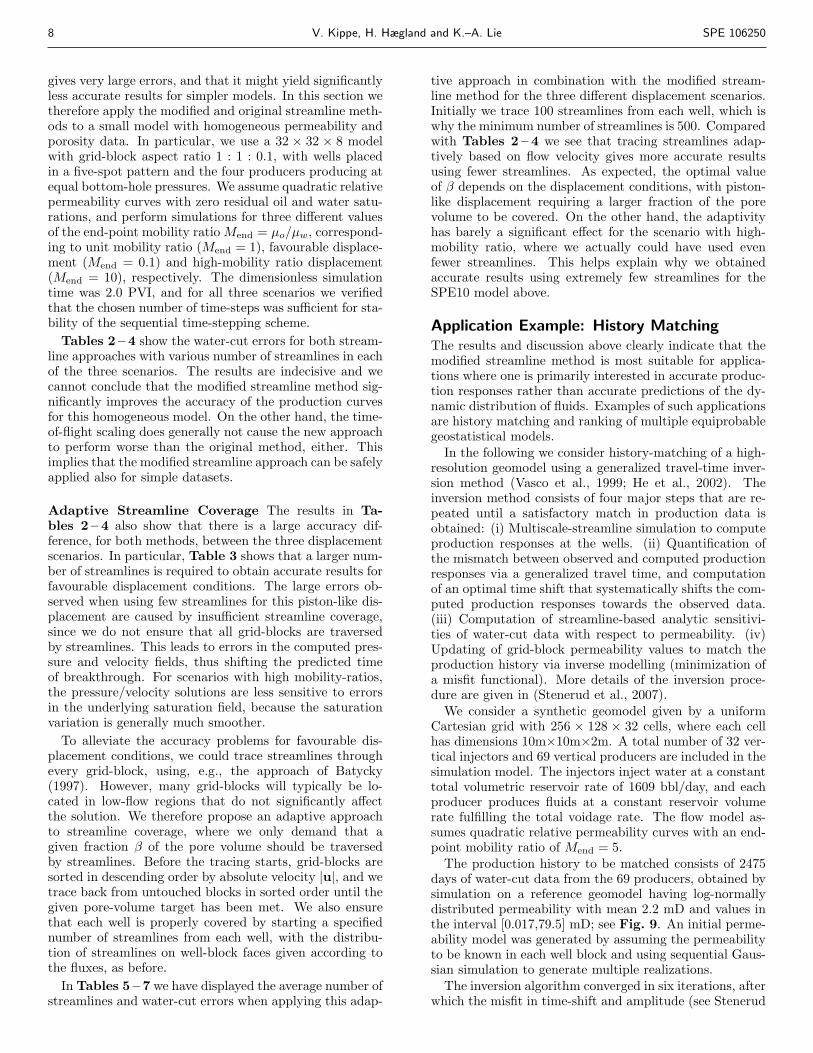
gives very large errors, and that it might yield significantlyless accurate results for simpler models. In this section wetherefore apply the modified and original streamline meth-ods to a small model with homogeneous permeability andporosity data. In particular, we use a 32 × 32 × 8 modelwith grid-block aspect ratio 1 : 1 : 0.1, with wells placedin a five-spot pattern and the four producers producing atequal bottom-hole pressures. We assume quadratic relativepermeability curves with zero residual oil and water satu-rations, and perform simulations for three different valuesof the end-point mobility ratio Mend = µo/µw, correspond-ing to unit mobility ratio (Mend = 1), favourable displace-ment (Mend = 0.1) and high-mobility ratio displacement(Mend = 10), respectively. The dimensionless simulationtime was 2.0 PVI, and for all three scenarios we verifiedthat the chosen number of time-steps was sufficient for sta-bility of the sequential time-stepping scheme.

Tables 2 – 4 show the water-cut errors for both stream-line approaches with various number of streamlines in eachof the three scenarios. The results are indecisive and wecannot conclude that the modified streamline method sig-nificantly improves the accuracy of the production curvesfor this homogeneous model. On the other hand, the time-of-flight scaling does generally not cause the new approachto perform worse than the original method, either. Thisimplies that the modified streamline approach can be safelyapplied also for simple datasets.

Adaptive Streamline Coverage The results in Ta-

bles 2 – 4 also show that there is a large accuracy dif-ference, for both methods, between the three displacementscenarios. In particular, Table 3 shows that a larger num-ber of streamlines is required to obtain accurate results forfavourable displacement conditions. The large errors ob-served when using few streamlines for this piston-like dis-placement are caused by insufficient streamline coverage,since we do not ensure that all grid-blocks are traversedby streamlines. This leads to errors in the computed pres-sure and velocity fields, thus shifting the predicted timeof breakthrough. For scenarios with high mobility-ratios,the pressure/velocity solutions are less sensitive to errorsin the underlying saturation field, because the saturationvariation is generally much smoother.

To alleviate the accuracy problems for favourable dis-placement conditions, we could trace streamlines throughevery grid-block, using, e.g., the approach of Batycky(1997). However, many grid-blocks will typically be lo-cated in low-flow regions that do not significantly affectthe solution. We therefore propose an adaptive approachto streamline coverage, where we only demand that agiven fraction β of the pore volume should be traversedby streamlines. Before the tracing starts, grid-blocks aresorted in descending order by absolute velocity |u|, and wetrace back from untouched blocks in sorted order until thegiven pore-volume target has been met. We also ensurethat each well is properly covered by starting a specifiednumber of streamlines from each well, with the distribu-tion of streamlines on well-block faces given according tothe fluxes, as before.

In Tables 5 – 7 we have displayed the average number ofstreamlines and water-cut errors when applying this adap-

tive approach in combination with the modified stream-line method for the three different displacement scenarios.Initially we trace 100 streamlines from each well, which iswhy the minimum number of streamlines is 500. Comparedwith Tables 2 – 4 we see that tracing streamlines adap-tively based on flow velocity gives more accurate resultsusing fewer streamlines. As expected, the optimal valueof β depends on the displacement conditions, with piston-like displacement requiring a larger fraction of the porevolume to be covered. On the other hand, the adaptivityhas barely a significant effect for the scenario with high-mobility ratio, where we actually could have used evenfewer streamlines. This helps explain why we obtainedaccurate results using extremely few streamlines for theSPE10 model above.

Application Example: History MatchingThe results and discussion above clearly indicate that themodified streamline method is most suitable for applica-tions where one is primarily interested in accurate produc-tion responses rather than accurate predictions of the dy-namic distribution of fluids. Examples of such applicationsare history matching and ranking of multiple equiprobablegeostatistical models.

In the following we consider history-matching of a high-resolution geomodel using a generalized travel-time inver-sion method (Vasco et al., 1999; He et al., 2002). Theinversion method consists of four major steps that are re-peated until a satisfactory match in production data isobtained: (i) Multiscale-streamline simulation to computeproduction responses at the wells. (ii) Quantification ofthe mismatch between observed and computed productionresponses via a generalized travel time, and computationof an optimal time shift that systematically shifts the com-puted production responses towards the observed data.(iii) Computation of streamline-based analytic sensitivi-ties of water-cut data with respect to permeability. (iv)Updating of grid-block permeability values to match theproduction history via inverse modelling (minimization ofa misfit functional). More details of the inversion proce-dure are given in (Stenerud et al., 2007).

We consider a synthetic geomodel given by a uniformCartesian grid with 256 × 128 × 32 cells, where each cellhas dimensions 10m×10m×2m. A total number of 32 ver-tical injectors and 69 vertical producers are included in thesimulation model. The injectors inject water at a constanttotal volumetric reservoir rate of 1609 bbl/day, and eachproducer produces fluids at a constant reservoir volumerate fulfilling the total voidage rate. The flow model as-sumes quadratic relative permeability curves with an end-point mobility ratio of Mend = 5.

The production history to be matched consists of 2475days of water-cut data from the 69 producers, obtained bysimulation on a reference geomodel having log-normallydistributed permeability with mean 2.2 mD and values inthe interval [0.017,79.5] mD; see Fig. 9. An initial perme-ability model was generated by assuming the permeabilityto be known in each well block and using sequential Gaus-sian simulation to generate multiple realizations.

The inversion algorithm converged in six iterations, afterwhich the misfit in time-shift and amplitude (see Stenerud


Fig. 9— Geomodels for the 3D history-matching case: ref-erence model (top) initial model (middle), and final match(bottom).

et al., 2007) were reduced to 7.8% and 53.7% of their initialvalues, respectively. In the inversion, we use the originalstreamline method with 500 000 streamlines and 15 uni-form pressure steps of 165 days for each forward simula-tion. To solve the pressure equation we use the multiscalemethod (MsMFEM) mentioned above. The total time forthe whole inversion was 43 minutes on a Linux worksta-tion with a 2.4 GHz Intel Core 2 Duo processor with 4Mbcache and 3 Gb memory. Using the modified streamlinemethod we were able to reduce the number of streamlinesto 50 000, and thereby reduce the total time for inversionto 17 minutes without reducing significantly the quality ofthe obtained history match. In fact, the time-shift and am-plitude residuals were reduced to 7.6% and 48.7% of theiroriginal values, respectively.

Concluding RemarksIn this paper we have introduced a modified streamlinemethod which greatly reduces the mass-balance errorswhen simulating large and complex reservoir models usingfew streamlines. Improved mass-conservation propertiesare achieved by locally scaling the time-of-flight grids, onwhich the one-dimensional transport equations are solved,to enforce mass conservation in the mappings between theEulerian pressure grid and the Lagrangian streamlines. Asa consequence, we are able to obtain accurate productioncurves on a million grid-block reservoir model with five

wells using only 5 000 streamlines, and the total simulationtime is less than ten minutes using a standard desktop com-puter. When coupling the modified streamline approachwith an efficient approximate pressure solution techniquethe simulation time was further reduced to less than twoand a half minutes.

We verified that the modified approach is applicable alsoto simple models by showing that its performance wassimilar to that of the original method on a homogeneousdataset. We also demonstrated that favourable, piston-like displacement might be challenging to simulate usingfew streamlines, and proposed an adaptive approach tostreamline coverage based on tracing streamlines from un-touched cells in high-flow regions until a given fraction ofthe pore volume has been traversed.

We have not considered improvements in the algorithmsfor mapping saturations between streamlines and the pres-sure grid, and the modified approach does therefore notgive significantly better saturation solutions than the orig-inal method. This implies that the modified streamlinemethod is best suited for applications that depend heavilyon rapid estimation of production responses. As an ex-ample we demonstrated significant speed-up for a history-match of a million grid-block model with 32 injectors and69 producers.

Finally, we remark that our modified method probablyhas an even larger potential for non-Cartesian grids, wherePollock’s method for analytical tracing of streamlines in-troduces large errors, both in the time-of-flights and inthe actual streamline paths; see Hægland et al. (2006) forfurther details.

NomenclatureRoman letters

A AreaC Constantf Fractional flowFIP Volume of fluid (water) in placeK Permeability tensorINJ Injected volume (water)kr Relative permeabilityMend End-point mobility ratiop PressurePRD Produced volume (water)s Distance along streamlineS SaturationSwc Connate water saturationSor Residual oil saturationt Timeu Total Darcy velocityV Volumew Water-cut curveq Volumetric rate

Greek letters

δ(·) Relative errorε Relative mass balance errorλ Mobilityµ Viscosityφ Porosityψ,χ Bi-streamfunctions


τ Time-of-flightζ Space coordinate along streamline

Subscripts

i Block numberj Phase numbersl Streamline numberst Streamtube numbero, w Oil and water phasest, tot Total∆t Time-step

AcknowledgementsThe authors are grateful to V. R. Stenerud for provid-ing the history-matching example, and to J. R. Natvig forproviding the plot of time-of-flight within a grid cell. Theauthors gratefully acknowledge financial support from theResearch Council of Norway; Kippe and Lie under grantsnumber 152732/S30 and 158908/I30, and Hægland undergrant number 173875/I30.

ReferencesJ. E. Aarnes and K.-A. Lie. Toward reservoir simulation on geo-

logical grid models. In Proceedings of the 9th European Con-ference on the Mathematics of Oil Recovery, Cannes, France,2004. EAGE.

J. E. Aarnes, V. Kippe, and K.-A. Lie. Mixed multiscale finiteelements and streamline methods for reservoir simulation oflarge geomodels. Adv. Water Resour., 28(3):257–271, 2005.

R.P. Batycky. A Three-Dimensional Two-Phase Field-ScaleStreamline Simulator. PhD thesis, Stanford University, Dept.of Petroleum Engineering, 1997.

J. Bear. Dynamics of Fluids in Porous Media. American Else-vier, New York, 1972.

F. Bradtvedt, K. Bratvedt, C.F. Buchholz, T. Gimse,H. Holden, L. Holden, R. Olufsen, and N.H. Risebro. Three-dimensional reservoir simulation based on front tracking.North Sea Oil and Gas Reservoirs, III:247–257, 1994.

F. Bratvedt, K. Bratvedt, C.F. Buchholz, T. Gimse, H. Holden,L. Holden, and N.H. Risebro. Frontline and frontsim: twofull-scale, two-phase, black oil reservoir simulators based onfront tracking. Surv. Math. Ind., (3):185–215, 1993.

M.A. Christie and M.J. Blunt. Tenth SPE comparative solutionproject: A comparison of upscaling techniques. SPE Reser-voir Eval. Eng., 4(4):308–317, 2001. url: www.spe.org/csp.

M. Crane, F. Bratvedt, K. Bratvedt, P. Childs, and R. Olufsen.A fully compositional streamline simulator. In SPE AnnualTechnical Conference and Exhibition, Dallas, TX, October 1- 4, 2000, SPE 63156, 2000.

A. Datta-Gupta and M. J. King. Streamline Simulation: Theoryand Practice. SPE Textbook Series. to appear.

G. Di Donato and M.J. Blunt. Streamline-based dual-porosity simulation of reactive transport and flow in frac-tured reservoirs. Water Resour. Res., 40(W04203), 2004.doi:10.1029/2003WR002772.

M.G. Gerritsen, K. Jessen, B.T. Mallison, and J. Lambers. Afully adaptive streamline framework for the challenging sim-ulation of gas-injection processes. In SPE Annual Technical

Conference and Exhibition, Houston, TX, October 9 - 12,2005, SPE 97270, 2005.

H. Hægland, H.K. Dahle, G.T. Eigestad, K.-A. Lie, andI. Aavatsmark. Improved streamlines and time-of-flight forstreamline simulation on irregular grids. Advances in WaterResources, 2006. doi:10.1016/j.advwatres.2006.09.002.

Z. He, A. Datta-Gupta, and S. Yoon. Streamline-based produc-toin data integration with gravity and changing field condi-tions. SPE J., 7(4):423–436, 2002.

H. Holden and N.H. Risebro. Front Tracking for HyperbolicConservation Laws, volume 152 of Applied Mathematical Sci-ences. Springer, New York, 2002.

E. Jimenez, K. Sabir, A. Datta-Gupta, and M.J. King. Spa-tial error and convergence in streamline simulation. In SPEReservoir Simulation Symposium, Houston, TX, January 31-February 2, 2005, SPE 92873, 2005.

M. J. King and A. Datta-Gupta. Streamline simulation: Acurrent perspective. In Situ, 22(1):91–140, 1998.

S.F. Matringe and M.G. Gerritsen. On accurate tracing ofstreamlines. In SPE Annual Technical Conference and Exhi-bition, Houston, TX, September 26 - 29, 2004, SPE 89920,2004.

S.F. Matringe, R. Juanes, and H.A. Tchelepi. Robust stream-line tracing for the simulation of porous media flow ongeneral triangular and quadrilateral grids. JCP, 2006.doi:10.1016/j.jcp.2006.07.004.

I.C. Pallister and D.K. Ponting. Asset optimization using mul-tiple realizations and streamline simulation. In SPE AsiaPacific Conference on Integrated Modelling for Asset Man-agement, Yokohama, Japan, 25 - 26 April 2000, SPE 59460,2000.

D.W. Pollock. Semi-analytical computation of path lines forfinite-difference models. Ground Water, 26(6):743–750, 1988.

D.K. Ponting. Hybrid streamline methods. In SPE Asia PacificConference on Integrated Modelling for Asset Management,Kuala Lumpur, Malaysia, 23 - 24 March 1998, SPE 39756,1998.

V.R. Stenerud, V. Kippe, A. Datta-Gupta, and K.-A. Lie.Adaptive multiscale streamline simulation and inversionfor high-resolution geomodels. In SPE Reservoir Simula-tion Symposium, Houston, TX, February 26–28, 2007, SPE106228, 2007.

K. Stuben. Algebraic Multigrid (AMG): An Introduction withApplications. Academinc Press, 2000. Guest appendix in thebook Multigrid by U. Trottenberg and C.W. Oosterlee andA. Schuller.

M.R. Thiele. Streamline simulation. In 8th International Forumon Reservoir Simulation, Stresa / Lago Maggiore, Italy, 20-24 June 2005.

M.R. Thiele, R.P. Batycky, and M.J. Blunt. A streamline-basedfield-scale compositional reservoir simulator. In SPE AnnualTechnical Conference and Exhibition, San Antonio, TX, Oc-tober 5 - 8, 1997, SPE 38889, 1997.

D.W. Vasco, S. Yoon, and A. Datta-Gupta. Integrating dy-namic data into high-resolution models using streamline-based analytic sensitivity coefficients. SPE J., pages 389–399,1999.


NSL Method P1 P2 P3 P4 δ(S) Tsl (s) Ttot (s)

100 000Original 8.91e-03 6.24e-03 2.44e-03 2.99e-03 2.75e-02 508.92 974.94Modified 9.86e-03 4.61e-03 1.97e-03 3.67e-03 2.83e-02 508.20 979.03





Table 1— Errors in water-cuts δ(w) for producers P1 to P4, saturation error δ(S), computational time for the streamline part of thesimulation Tsl, and total computation time Ttot for the original and modified streamline methods on the SPE10 model for variousnumber of streamlines (NSL).

NSL O/M P1 P2 P3 P4

2000O 5.07e-02 2.33e-02 3.11e-02 2.90e-02M 3.93e-02 2.52e-02 2.69e-02 2.89e-02

1750O 4.31e-02 2.86e-02 3.30e-02 2.86e-02M 3.64e-02 2.18e-02 2.37e-02 2.23e-02

1500O 5.08e-02 2.91e-02 4.59e-02 3.21e-02M 5.11e-02 3.92e-02 3.15e-02 3.82e-02

1250O 6.66e-02 5.21e-02 6.25e-02 5.49e-02M 6.30e-02 3.51e-02 4.55e-02 3.92e-02

1000O 5.56e-02 4.33e-02 5.78e-02 3.97e-02M 4.73e-02 3.76e-02 5.00e-02 4.09e-02

750O 9.25e-02 8.73e-02 9.09e-02 9.17e-02M 7.37e-02 7.03e-02 5.47e-02 7.30e-02

500O 1.44e-01 1.12e-01 1.06e-01 1.15e-01M 1.19e-01 9.82e-02 9.64e-02 1.10e-01

250O 1.68e-01 2.15e-01 2.43e-01 2.19e-01M 1.49e-01 1.61e-01 1.77e-01 1.59e-01

Table 2— Water-cut errors, δ(w), on the homogeneous modelfor the original (O) and modified (M) versions of the stream-line method, when the end-point mobility ratio Mend = 1.

NSL O/M P1 P2 P3 P4

2000O 4.56e-02 9.18e-02 8.97e-02 9.46e-02M 4.43e-02 9.30e-02 8.97e-02 9.47e-02

1750O 3.29e-02 6.53e-02 6.78e-02 5.17e-02M 3.07e-02 6.44e-02 7.09e-02 5.08e-02

1500O 7.01e-02 1.20e-01 8.98e-02 1.05e-01M 5.27e-02 1.13e-01 8.96e-02 1.04e-01

1250O 6.76e-02 1.13e-01 1.42e-01 8.19e-02M 4.60e-02 1.09e-01 1.42e-01 6.32e-02

1000O 1.40e-01 1.62e-01 1.76e-01 1.67e-01M 1.39e-01 1.62e-01 1.76e-01 1.67e-01

750O 3.40e-01 3.14e-01 3.39e-01 3.57e-01M 3.39e-01 3.15e-01 3.40e-01 3.57e-01

500O 4.26e-01 4.50e-01 4.65e-01 4.69e-01M 4.25e-01 4.34e-01 4.64e-01 4.61e-01

250O 7.79e-01 8.20e-01 8.44e-01 7.99e-01M 7.86e-01 8.17e-01 8.42e-01 8.00e-01

Table 3— Water-cut errors, δ(w), on the homogeneous modelfor the original (O) and modified (M) versions of the stream-line method, when the end-point mobility ratio Mend = 0.1.

NSL O/M P1 P2 P3 P4

2000O 2.55e-02 1.33e-02 5.36e-02 1.35e-02M 2.58e-02 2.45e-02 2.33e-02 8.44e-03

1750O 2.89e-02 1.36e-02 6.15e-02 1.04e-02M 2.78e-02 1.94e-02 2.63e-02 8.13e-03

1500O 3.37e-02 1.79e-02 4.43e-02 1.92e-02M 3.14e-02 1.00e-02 3.88e-02 9.23e-03

1250O 3.93e-02 2.42e-02 4.93e-02 2.60e-02M 2.63e-02 2.61e-02 5.36e-02 2.72e-02

1000O 5.33e-02 6.55e-02 3.33e-02 3.19e-02M 6.68e-02 2.29e-02 5.79e-02 4.14e-02

750O 5.05e-02 3.52e-02 4.68e-02 4.27e-02M 5.84e-02 2.73e-02 5.09e-02 4.79e-02

500O 6.97e-02 3.53e-02 5.19e-02 4.42e-02M 3.49e-02 4.35e-02 5.22e-02 3.14e-02

250O 7.07e-02 9.37e-02 1.04e-01 1.01e-01M 7.42e-02 9.58e-02 1.20e-01 8.96e-02

Table 4— Water-cut errors, δ(w), on the homogeneous modelfor the original (O) and modified (M) versions of the stream-line method, when the end-point mobility ratio Mend = 10.

β NSL P1 P2 P3 P41.0 875 3.54e-02 3.08e-02 2.50e-02 3.92e-020.9 714 3.86e-02 3.35e-02 3.14e-02 3.89e-020.8 576 4.74e-02 3.11e-02 2.28e-02 3.07e-020.7 500 6.88e-02 5.88e-02 7.22e-02 4.83e-020.6 500 6.83e-02 6.37e-02 7.03e-02 5.09e-02

Table 5— Average number of streamlines and water-cut er-rors, δ(w), on the homogeneous model for various values of β,when the end-point mobility ratio Mend = 1.


Table 6— Average number of streamlines and water-cut er-rors, δ(w), on the homogeneous model for various values of β,when the end-point mobility ratio Mend = 0.1.



Table 7— Average number of streamlines and water-cut er-rors, δ(w), on the homogeneous model for various values of β,when the end-point mobility ratio Mend = 10.

Documents

SPE 106250 A Method to Improve the Mass Balance in ...folk.ntnu.no/andreas/papers/SPE106250.pdfA Method to Improve the Mass Balance in Streamline Methods Vegard Kippe, ... (permeability,