SPE-169479-MS

Evaluation of Strategies for Enhancing Production of Low-ViscosityLiquids From Tight/Shale Reservoirs

George J. Moridis, Lawrence Berkeley National Laboratory; Thomas A. Blasingame, Texas A&M University

Copyright 2014, Society of Petroleum Engineers

This paper was selected for presentation by an SPE program committee following review of information contained in an abstract submitted by the author(s). Contentsof the paper have not been reviewed by the Society of Petroleum Engineers and are subject to correction by the author(s). The material does not necessarily reflectany position of the Society of Petroleum Engineers, its officers, or members. Electronic reproduction, distribution, or storage of any part of this paper without the writtenconsent of the Society of Petroleum Engineers is prohibited. Permission to reproduce in print is restricted to an abstract of not more than 300 words; illustrations maynot be copied. The abstract must contain conspicuous acknowledgment of SPE copyright.

Abstract

Production of low-viscosity liquids (including condensates) from tight reservoirs (such as shales) isseverely restricted by the ultra low-permeability of such formations, limiting production to a very smallfraction (usually less than 5 percent) of the liquids-in-place. In this study, which is part of a widerinvestigation, we evaluate by means of numerical simulation several possible strategies to enhancelow-viscosity liquids production from such reservoirs. These strategies include (a) physical displacementprocesses, (b) non-thermal processes to reduce the viscosity and the critical saturation of the liquids, (c)thermal processes, (d) enhanced reservoir stimulation, (e) novel well configurations and (f) combinationsthereof. The objectives of this effort are to (1) to remove from further consideration potential productionstrategies that hold limited (if any) promise, and (2) to identify production strategies that appear to havepotential for further study and development.

We first determine the baseline production performance of such reservoirs corresponding to severalreference production regimes that involve minimal or no reservoir stimulation, standard displacementfluids (H2O or CH4), standard well configurations and no thermal treatment. We then evaluate theefficiency of several production strategies: (a) traditional continuous gas flooding using parallel horizontalwells and using the currently abundant shale gas, (b) water-alternating-gas (WAG) flooding, (c) huff-and-puff injection/production strategies using lean gas/rich gas in a traditional (single) horizontal wellwith multiple fractures, (d) flooding using appropriate gases (e.g., CO2, N2, CH4) using appropriate wellconfigurations (mainly horizontal), with the viscosity reduction resulting from the gas dissolution into theliquids, and (e) thermal processes, in which the viscosity reduction is achieved by heating, possibly to thepoint of liquid vaporization and transport through the matrix to the production wells as a gas. Our studyincludes an analysis of the sensitivity of the liquids production to the main parameters defining each ofthe strategies listed above in an effort to determine the critically important parameters and factors thatcontrol the production performance and efficiency.

IntroductionBackgroundGas production from tight gas/shale gas reservoirs over the last decade has met with spectacular successwith the advent of advanced reservoir stimulation techniques (mainly hydraulic fracturing), to the extent

This paper was prepared for presentation at the SPE Latin American and Caribbean Petroleum Engineering Conference held in Maracaibo, Venezuela, 21–23 May2014.

that shale gas is now among the main contributors to US hydrocarbon production. This remarkable successhas not been matched by similar progress in the production of (relatively) low-viscosity liquid hydrocar-bons (including condensates) because of the significant challenges to liquid flow posed by the ultra-lowpermeability (and the correspondingly high capillary pressures and irreducible liquids saturations) of suchreservoirs. These difficulties have limited liquids production to a very low fraction (usually �5%) of theresources-in-place.

Increasing the recovery of liquids from these ultra-low permeability systems even by 50-100 percentover its current very low levels (to a level that is still low in absolute terms, but very significant in relative(hence, economic) terms) not only will increase production and earnings, but will have considerable widereconomic implications, as the enhanced recovery will affect reserves and the valuation of companies. Oureffort aims to address this issue by using numerical simulation to investigate a wide range of possiblestrategies for improved liquids production from tight/shale reservoirs. In essence, this is an attempt toprovide a baseline “mechanistic” study that deploys some state-of-the-art tools in reservoir modeling. Ifsuccessful in identifying interactions, processes and methods that can increase production by as little as50-100 percent over the current low recovery rates (usually 5% or less), the impact in the industry can besignificant and potentially dramatic (despite a recovery that may remain low in absolute terms) not onlybecause of an increase in hydrocarbon recovery, but also because this can allow an increase in reserveestimation and company valuation, with considerable economic consequences. In short, the extremely lowoil recovery of these systems warrants the identification of key processes and interactions, and thedevelopment of strategies to achieve maximum recovery. The current effort aims to address these issues.

ObjectivesThe main problem that this study addresses is the extremely low liquid hydrocarbon production from“light/tight oil” systems. The overall objective of the effort (of which the study reported in this part is apart) is to to identify, analyze and quantify by means of numerical simulation the dominant interactions(fluid-fluid, fluid-media, fluid-fractures, etc.) that underlie and control the processes involved in theproduction (by various methods) of low-viscosity hydrocarbons from tight (shale) media, and to use thegained insights to increase/optimize production. The specific objectives are:

● To identify and quantitatively describe mechanisms that control fluid flow and the various systeminteractions in tight media, and to quantitatively describe the behavior of the several fluidsinvolved in the production process through the extremely small pore space of tight media, leadingto promising strategies for enhanced recovery.

● To identify production strategies that hold limited (if any) promise, and remove them from furtherconsideration potential.

● To identify and focus on strategies that appear to have potential for significant enhancement ofhydrocarbon production (in terms of maximization of both production and recovery), to numeri-cally evaluate their large-scale and long-term performance, to identify the dominant mechanismand processes, and evaluate the relative importance of the properties, conditions and parametersthat control them.

● Based on insights provided by the various analyses, to propose (if possible) novel approaches asnew methods for enhanced production of low-viscosity fluids from tight/shale oil reservoirs.

The studies in this paper focus on scoping calculations that aim to determine the baseline performanceof various key production methods that are considered “standard” in the attempt to produce low-viscosityliquids from tight- and shale-oil reservoirs. These include recovery using displacement methods, viscosityreduction methods (thermal processes and those caused by the dissolution of appropriate substances, suchas CO2), enhanced reservoir stimulation, and combinations thereof.

2 SPE-169479-MS

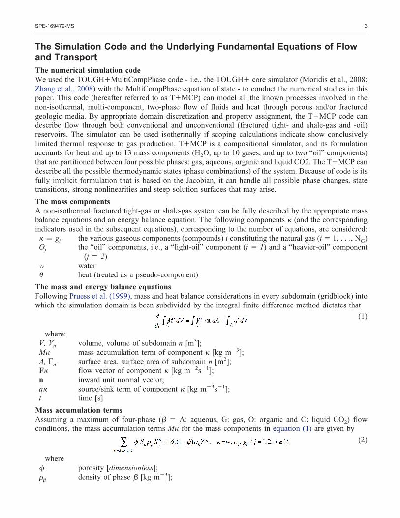
The Simulation Code and the Underlying Fundamental Equations of Flowand TransportThe numerical simulation codeWe used the TOUGH�MultiCompPhase code - i.e., the TOUGH� core simulator (Moridis et al., 2008;Zhang et al., 2008) with the MultiCompPhase equation of state - to conduct the numerical studies in thispaper. This code (hereafter referred to as T�MCP) can model all the known processes involved in thenon-isothermal, multi-component, two-phase flow of fluids and heat through porous and/or fracturedgeologic media. By appropriate domain discretization and property assignment, the T�MCP code candescribe flow through both conventional and unconventional (fractured tight- and shale-gas and -oil)reservoirs. The simulator can be used isothermally if scoping calculations indicate show conclusivelylimited thermal response to gas production. T�MCP is a compositional simulator, and its formulationaccounts for heat and up to 13 mass components (H2O, up to 10 gases, and up to two “oil” components)that are partitioned between four possible phases: gas, aqueous, organic and liquid CO2. The T�MCP candescribe all the possible thermodynamic states (phase combinations) of the system. Because of code is itsfully implicit formulation that is based on the Jacobian, it can handle all possible phase changes, statetransitions, strong nonlinearities and steep solution surfaces that may arise.

The mass componentsA non-isothermal fractured tight-gas or shale-gas system can be fully described by the appropriate massbalance equations and an energy balance equation. The following components � (and the correspondingindicators used in the subsequent equations), corresponding to the number of equations, are considered:� � gi the various gaseous components (compounds) i constituting the natural gas (i � 1, . . ., NG)Oj the “oil” components, i.e., a “light-oil” component (j � 1) and a “heavier-oil” component

(j � 2)w water� heat (treated as a pseudo-component)

The mass and energy balance equationsFollowing Pruess et al. (1999), mass and heat balance considerations in every subdomain (gridblock) intowhich the simulation domain is been subdivided by the integral finite difference method dictates that

(1)

where:V, Vn volume, volume of subdomain n [m3];M� mass accumulation term of component � [kg m�3];A, �n surface area, surface area of subdomain n [m2];F� flow vector of component � [kg m�2s�1];n inward unit normal vector;q� source/sink term of component � [kg m�3s�1];t time [s].

Mass accumulation termsAssuming a maximum of four-phase (� � A: aqueous, G: gas, O: organic and C: liquid CO2) flowconditions, the mass accumulation terms M� for the mass components in equation (1) are given by

(2)

where� porosity [dimensionless];�� density of phase � [kg m�3];

SPE-169479-MS 3

S� saturation of phase � [dimensionless];mass fraction of component � � w, gi, oj in phase � [kg/kg]

�R rock density [kg m�3];Ygi mass of sorbed gaseous component gi per unit mass of rock [kg/kg]�S � 1 for shales and 0 for non-sorbing tight-gas system (usually devoid of substantial organic

carbon)The first term in equation (2) describes fluid mass stored in the pores, and the second the mass of

gaseous components sorbed onto the organic carbon (mainly kerogen) content of the matrix of the porousmedium. Although gas desorption from kerogenic media has been studied extensively in coalbed methanereservoirs, and several analytic/semi-analytic models have been developed for such reservoirs (Clarksonand Bustin, 1999), the sorptive properties of shale are not necessarily analogous to coal (Schettler andParmely, 1991). The most commonly used empirical model describing sorption onto organic carbon inshales is analogous to that used in coalbed methane and follows the Langmuir isotherm that, for asingle-component gas, is described by

(3)

The mL term equation (3) describes the total mass storage of component gi at infinite pressure (kg ofgas/kg of matrix material), pL is the pressure at which half of this mass is stored (Pa), and kL is a kineticconstant of the Langmuir sorption (1/s). In most studies applications, an instantaneous equilibrium isassumed to exist between the sorbed and the free gas, i.e., there is no transient lag between pressurechanges and the corresponding sorption/desorption responses and the equilibrium model of Langmuirsorption is assumed to be valid (Figure 6). Although this appears to be a good approximation in shales(Gao et al., 1994) because of the very low permeability of the matrix (onto which the various gascomponents are sorbed), the subject has not been fully investigated. For multi-component gas, equation(3) becomes

(4)

where Bgi is the Langmuir constant of component gi in 1/Pa (Pan et al., 2008), and ygi is thedimensionless mole fraction of the gas component.

Heat accumulation termsThe heat accumulation term includes contributions from the rock matrix and all the phases, and is givenby the equation

(5)

where:CR heat capacity of the dry rock [J kg�1 K�1];U� specific internal energy of phase � [J kg�1];ugi specific internal energy of sorbed component gi [J kg�1];T temperature [K]

4 SPE-169479-MS

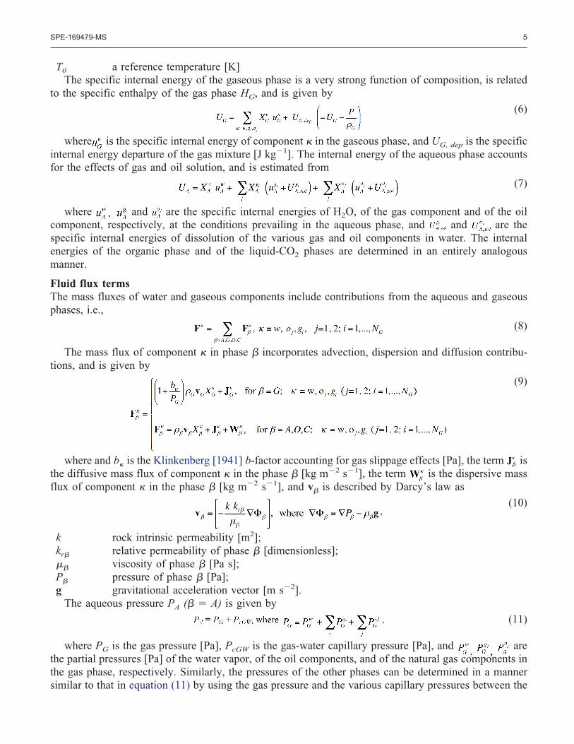
T0 a reference temperature [K]The specific internal energy of the gaseous phase is a very strong function of composition, is related

to the specific enthalpy of the gas phase HG, and is given by

(6)

where is the specific internal energy of component � in the gaseous phase, and UG, dep is the specificinternal energy departure of the gas mixture [J kg�1]. The internal energy of the aqueous phase accountsfor the effects of gas and oil solution, and is estimated from

(7)

where and are the specific internal energies of H2O, of the gas component and of the oilcomponent, respectively, at the conditions prevailing in the aqueous phase, and and are thespecific internal energies of dissolution of the various gas and oil components in water. The internalenergies of the organic phase and of the liquid-CO2 phases are determined in an entirely analogousmanner.

Fluid flux termsThe mass fluxes of water and gaseous components include contributions from the aqueous and gaseousphases, i.e.,

(8)

The mass flux of component � in phase � incorporates advection, dispersion and diffusion contribu-tions, and is given by

(9)

where and b� is the Klinkenberg [1941] b-factor accounting for gas slippage effects [Pa], the term isthe diffusive mass flux of component � in the phase � [kg m�2 s�1], the term is the dispersive massflux of component � in the phase � [kg m�2 s�1], and v� is described by Darcy’s law as

(10)

k rock intrinsic permeability [m2];kr� relative permeability of phase � [dimensionless];�� viscosity of phase � [Pa s];P� pressure of phase � [Pa];g gravitational acceleration vector [m s�2].

The aqueous pressure PA (� � A) is given by

(11)

where PG is the gas pressure [Pa], PcGW is the gas-water capillary pressure [Pa], and arethe partial pressures [Pa] of the water vapor, of the oil components, and of the natural gas components inthe gas phase, respectively. Similarly, the pressures of the other phases can be determined in a mannersimilar to that in equation (11) by using the gas pressure and the various capillary pressures between the

SPE-169479-MS 5

gas and the phase in question. The gas solubility in the aqueous phase is related to through Henry’slaw,

(12)

where Hgi � Hgi (T) [Pa] is a temperature-dependent factor akin to Henry’s constant. Note that it ispossible to determine the from the equality of fugacities in the aqueous and the gas phase. Althoughthis approach provides a more accurate solution, the difference provides a small increase in accuracy thatcannot justify the significantly larger execution time. The dissolution of the oil components in water, andof water in the oil components is described by the parametric relationships discussed by Falta et al. (1995)and found in Poling et al. (2001). The solubility of gases in oil components of the organic phase, as wellas all thermophysical properties of the oil components and of the organic phase above, at and below thebubble point, are described using the relationships recommended by McCain et al. (2011). The solubilityof gases in the liquid CO2-phase and the corresponding thermophysical properties are computed usingsimple parametric equations, but there is very little information on the subject.

The term is the diffusive mass flux of component � in the phase � [kg m�2 s�1] that is describedby

(13)

where is the multicomponent molecular diffusion coefficient of component � in the gas phase in theabsence of a porous medium [m2 s�1], and � is the tortuosity of phase � [dimensionless] computed fromthe Millington and Quirk [1961] model. The diffusive mass fluxes of the water vapor, the oil vapors, andthe gases in the gas phase are related through the relationship of Bird et al. [1960]

(14)

which ensures that the total diffusive mass flux of the gas phase is zero with respect to the mass averagevelocity when summed over the components. Then the total gas phase mass flux is the product of thevelocity and density of the gas phase.

The term is the dispersive mass flux [kg m�2 s�1] of component � in phase � (�A,O,C) that isdescribed by

(15a)

where is the dispersion tensor of component � in phase �,

(15b)

and are the transverse and longitudinal dispersivities of component � in phase � [m], is thelength of the velocity vector, and all other terms are as previously defined.

In media with nano-scale pores (such as shales), the Klinkenberg b-factor is computed using themethod of Florence et al. (2007) and Freeman et al. (2009) from the equation

(16)

where Kn is the Knudsen diffusion number (dimensionless), which accounts for the effects of the meanfree path of gas molecules being on the same order as the pore dimensions of the porous media andcharacterizes the deviation from continuum flow. Knudsen diffusion can be very important in porous

6 SPE-169479-MS

media with very small pores (on the order of a few micrometers or smaller) and at low pressures. It iscomputed from (Freeman et al., 2009b) as

(17)

with M being the molecular weight and T the temperature (°K). The term � is determined fromKarniadakis and Beskok (2001) as

(18)

from Karniadakis and Beskok (2001).

Non-Darcy flowIf the flow is non-Darcian (e.g., in the case of fast gas flow in fractures), then equation (9) still applies,but v� is now computed from the solution of the quadratic equation

(19)

in which ��T is the “turbulence correction factor” (Katz et al., 1959). The quadratic equation in (19)is the general momentum-balance Forchheimer equation (Forchheimer, 1901; Wattenbarger and Ramey,1968), and incorporates laminar, inertial and turbulent effects. Its solution is

(20)

and v� from equation (20) is then used in the equations (9) of flow.

Heat fluxThe heat flux accounts for conduction, advection and radiative heat transfer, and is given by

(21)

Wherea representative thermal conductivity of the fluid-impregnated rock [W m�1 K�1];

h� specific enthalpy of phase � [J kg�1];f� radiance emittance factor [dimensionless];�0 Stefan-Boltzmann constant [5.6687 � 10�8 J m�2 K�4].

The specific enthalpy of the gas phase is computed as

(22)

where is the specific enthalpy of component � in the gaseous phase, and Hdep is the specific enthalpydeparture of the gas mixture [J kg�1]. The specific enthalpy of the aqueous phase is estimated from

(23)

where and are the specific enthalpies [J/kg] of H2O, of the gas component and of the oilcomponent, respectively, at the conditions prevailing in the aqueous phase, and and are thespecific enthalpies of dissolution of the various gas and oil components in water. The enhalpies of theorganic and of the liquid-CO2 phases are computed in a manner that entirely analogous to that of equation(23).

SPE-169479-MS 7

Source and sink terms In sinks with specified mass production rate, withdrawal of the mass component� is described by

(23)

where q� is the production rate of the phase � [kg m�3]. For a prescribed production rate, the phaseflow rate q� is determined from the phase mobility at the location of the sink. For source terms (wellinjection), the addition of a mass component � occurs at desired rates q �. The contribution of the injectedor produced fluids to the heat balance of the system are described by

(24)

where q� is the rate of heat addition or withdrawal in the course of injection or production, respectively(W/kg).

P- and T-dependence of � and kThe effect of pressure change on the porosity of the matrix is described by two options. The first involvesthe standard exponential equation

(25)

where �T is the thermal expansivity of the porous medium (1/K) and �p is the pore compressibility(1/Pa), which can be either a fixed number or a function of pressure (Moridis et al., 2008). A second optiondescribes the p-dependence of � as a polynomial function of p. The � - k relationship in the matrixisdescribed by the general expression of Rutqvist and Tsang (2003) as:

(26)

where is an empirical permeability reduction factor that ranges between 5 (for soft unconsolidatedmedia) and 29 (for lithified, highly consolidated media). Note that the equations described here are rathersimple and apply to matrix � and k changes when the changes in p and T are relatively small. Theseequations are not applicable when large pressure and temperature changes occur in the matrix, cannotdescribe the creation of new (secondary) fractures and cannot describe the evolution of the characteristicsof primary and secondary fractures (e.g., aperture, permeability, extent, surface area) over time as the fluidpressures, the temperatures, the fluid saturations and the stresses change. For such problems, it isnecessary to use the T�M model (Kim and Moridis, 2013) that couples the flow-and-thermal-processT�RW simulator discussed here with the ROCMECH geomechanical code. This coupled model accountsfor the effect of changing fluid pressures, saturations, stresses, and temperatures on the geomechanicalregime and provides an accurate description of the evolution of � and k over the entire spectrum of p andT covered during the simulation.

Fractured System Description and Subdomain Representation

Subdomains and fracturesThe fractured system in producing tight- and shale-gas reservoirs can be described as a set of interactingsubdomains (Moridis et al. 2010). These include the following:

● Subdomain 1 (S1): The original (i.e., in its undisturbed state prior to the initiation of productionoperations) reservoir rock, which may be naturally fractured and may be characterized by distinctsets of fractures, each one with its own properties (aperture, length, orientation, density, etc.). Theoriginal fractures in S1 are hereafter referred to as native fractures (NF).

8 SPE-169479-MS

● Subdomain 2 (S2): The fractures or fractured network created during the reservoir stimulation(e.g., by hydro-fracturing the reservoir rock). These artificial fractures penetrate Subdomain 1,increase the surface area from which can be produced, and may intercept the natural fractures ofSubdomain 1, thus providing access of gas in these fractures to the well. The fractures ofSubdomain 1 are expected to be the dominant pathways of flow to the well and are referred to asprimary fractures (PF).

● Subdomain 3 (S3): This is the subdomain defined by the stress-release fractures that are inducedby changes in the geomechanical status of the rock in the vicinity of the PF following the reservoirstimulation process. Their orientation is a function of the stress distribution and geomechanicalpropeties of the rock, but tend to occur on planes that are roughly perpendicular (ar at an angle)to the PF. Such fractures are referred to as secondary fractures (SF): they penetrate Subdomain 1mainly adjacent PFs (i.e., they occur within the fracture spacing, and, in their upper limit, they cancover it entirely), and intercepts native and primary fractures, thus increasing the flow area and,consequently, production.

● Subdomain 4 (S4): This is the subdomain defined by the stress-release fractures that are inducedby changes in the geomechanical status of the rock in the immediate vicinity of the wellborebecause of drilling. S4 is expected to have a roughly cylindrical shape centered around thewellbore axis, and to be characterized by a limited radius (i.e., short fracture length), high fracturedensity and small aperture. Thus, S4 is expected to represent a small fraction of the overall systemvolume, but may be important to flow as they can increase significantly the flow area, in additionto being directly connected to S1 and S2, and possibly intersecting fractures in S3. The fracturesin S4 are hereafter referred to as radial fractures (RF).

Thus, S1 is that natural (at discovery) state of the system. Drilling and well installations may inevitablycause S4 to form. S2 is the result of reservoir stimulation activities (and the only one over which theoperator can exert control), while S3 is a direct byproduct of them. S1 cannot provide sufficiently highproduction rates without stimulation in tight- and shale-gas reservoirs because of very low permeability.For the same fracture characteristics (except fracture length), production is maximized when the cumu-lative size of S2, S3 and S4 is maximized.

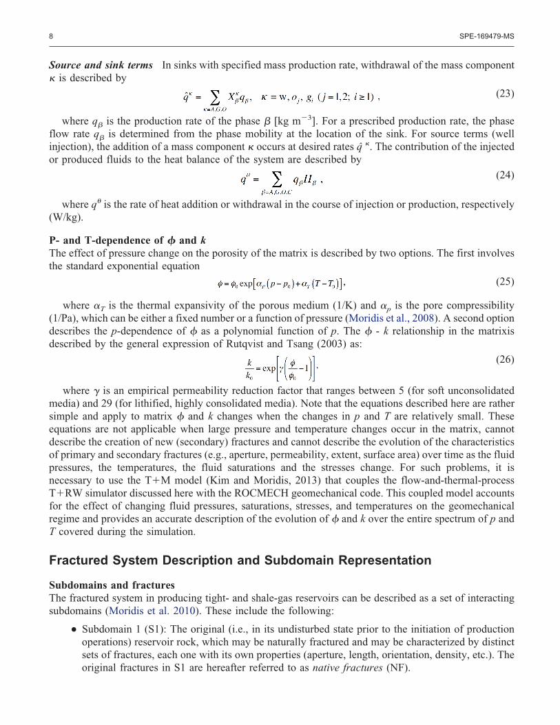
Types of fractured systemsBased on the properties and characteristics of S1 and the occurrence (or absence) of S3, there are fourpossible types of producing tight- or shale-gas reservoir systems. These are depicted in Figures 1 to 4 (allof which involve a horizontal well configuration), and are listed below in order of increasing complexity(in terms of description, simulation and analysis):

1. Type I (Figure 1): This is characterized by (a) the absence of NF fractures in S1, which nowinvolves the unfractured matrix, and (b) the absence of the S3 subdomain. This is the simplest andleast productive system, as it is characterized by the minimum surface area and flow pathways forpath production. It is possible to further simplify it by assuming absence of the S4 subdomain andof the RF.

2. Type II (Figure 2): Unlike Type I, Type II systems feature the S3 subdomain and SF. This isexpected to yield higher gas production because of increased surface area and more pathways toflow. SF can extend along the entire length of the fracture spacing (i.e., dsf�df, in which caseproduction is expected to be maximized).

3. Type III (Figure 3): The difference between Type I and Type III systems is the occurrence of thenative fractures (NF) in S1. Such a system is expected to have higher gas production than TypeI systems. Comparison of its productivity to Type II is not straightforward, because production is

SPE-169479-MS 9

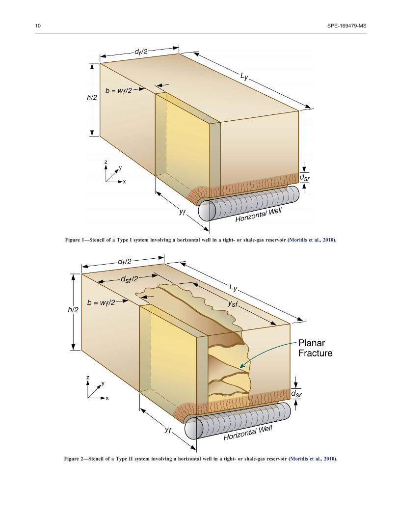
Figure 1—Stencil of a Type I system involving a horizontal well in a tight- or shale-gas reservoir (Moridis et al., 2010).

Figure 2—Stencil of a Type II system involving a horizontal well in a tight- or shale-gas reservoir (Moridis et al., 2010).

10 SPE-169479-MS

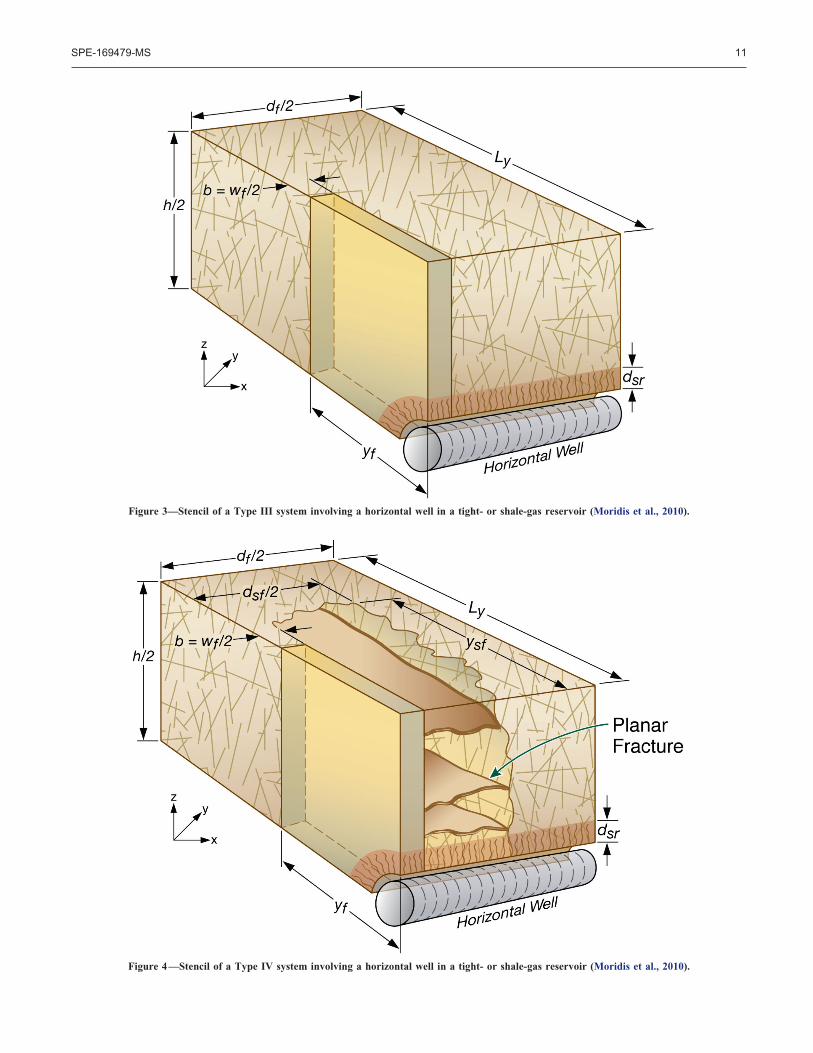
Figure 3—Stencil of a Type III system involving a horizontal well in a tight- or shale-gas reservoir (Moridis et al., 2010).

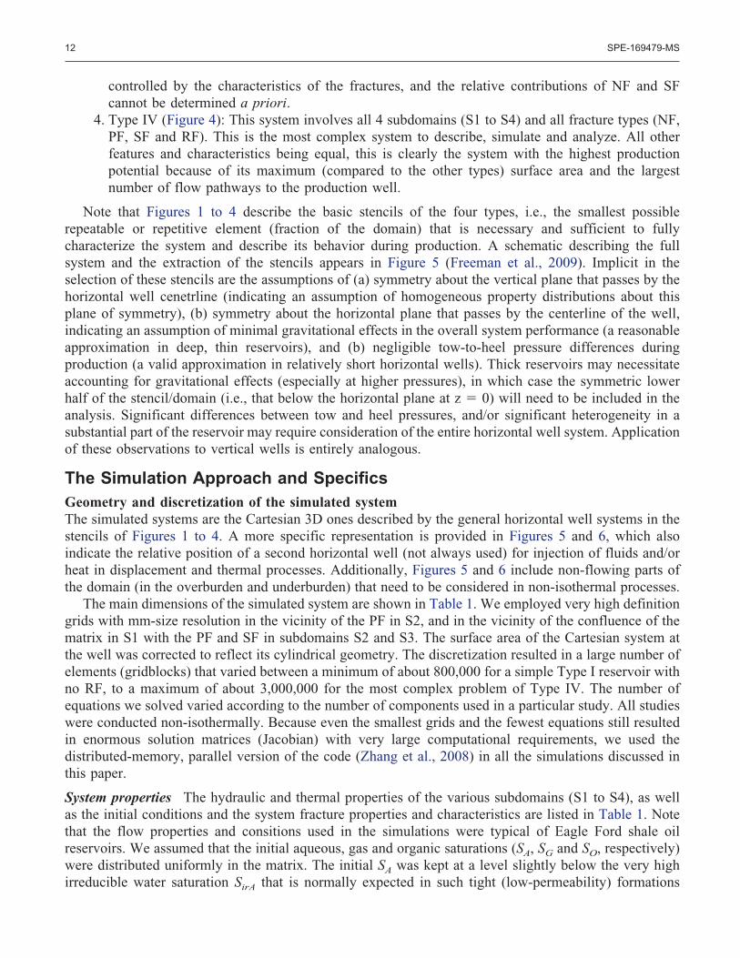
Figure 4—Stencil of a Type IV system involving a horizontal well in a tight- or shale-gas reservoir (Moridis et al., 2010).

SPE-169479-MS 11

controlled by the characteristics of the fractures, and the relative contributions of NF and SFcannot be determined a priori.

4. Type IV (Figure 4): This system involves all 4 subdomains (S1 to S4) and all fracture types (NF,PF, SF and RF). This is the most complex system to describe, simulate and analyze. All otherfeatures and characteristics being equal, this is clearly the system with the highest productionpotential because of its maximum (compared to the other types) surface area and the largestnumber of flow pathways to the production well.

Note that Figures 1 to 4 describe the basic stencils of the four types, i.e., the smallest possiblerepeatable or repetitive element (fraction of the domain) that is necessary and sufficient to fullycharacterize the system and describe its behavior during production. A schematic describing the fullsystem and the extraction of the stencils appears in Figure 5 (Freeman et al., 2009). Implicit in theselection of these stencils are the assumptions of (a) symmetry about the vertical plane that passes by thehorizontal well cenetrline (indicating an assumption of homogeneous property distributions about thisplane of symmetry), (b) symmetry about the horizontal plane that passes by the centerline of the well,indicating an assumption of minimal gravitational effects in the overall system performance (a reasonableapproximation in deep, thin reservoirs), and (b) negligible tow-to-heel pressure differences duringproduction (a valid approximation in relatively short horizontal wells). Thick reservoirs may necessitateaccounting for gravitational effects (especially at higher pressures), in which case the symmetric lowerhalf of the stencil/domain (i.e., that below the horizontal plane at z � 0) will need to be included in theanalysis. Significant differences between tow and heel pressures, and/or significant heterogeneity in asubstantial part of the reservoir may require consideration of the entire horizontal well system. Applicationof these observations to vertical wells is entirely analogous.

The Simulation Approach and SpecificsGeometry and discretization of the simulated systemThe simulated systems are the Cartesian 3D ones described by the general horizontal well systems in thestencils of Figures 1 to 4. A more specific representation is provided in Figures 5 and 6, which alsoindicate the relative position of a second horizontal well (not always used) for injection of fluids and/orheat in displacement and thermal processes. Additionally, Figures 5 and 6 include non-flowing parts ofthe domain (in the overburden and underburden) that need to be considered in non-isothermal processes.

The main dimensions of the simulated system are shown in Table 1. We employed very high definitiongrids with mm-size resolution in the vicinity of the PF in S2, and in the vicinity of the confluence of thematrix in S1 with the PF and SF in subdomains S2 and S3. The surface area of the Cartesian system atthe well was corrected to reflect its cylindrical geometry. The discretization resulted in a large number ofelements (gridblocks) that varied between a minimum of about 800,000 for a simple Type I reservoir withno RF, to a maximum of about 3,000,000 for the most complex problem of Type IV. The number ofequations we solved varied according to the number of components used in a particular study. All studieswere conducted non-isothermally. Because even the smallest grids and the fewest equations still resultedin enormous solution matrices (Jacobian) with very large computational requirements, we used thedistributed-memory, parallel version of the code (Zhang et al., 2008) in all the simulations discussed inthis paper.

System properties The hydraulic and thermal properties of the various subdomains (S1 to S4), as wellas the initial conditions and the system fracture properties and characteristics are listed in Table 1. Notethat the flow properties and consitions used in the simulations were typical of Eagle Ford shale oilreservoirs. We assumed that the initial aqueous, gas and organic saturations (SA, SG and SO, respectively)were distributed uniformly in the matrix. The initial SA was kept at a level slightly below the very highirreducible water saturation SirA that is normally expected in such tight (low-permeability) formations

12 SPE-169479-MS

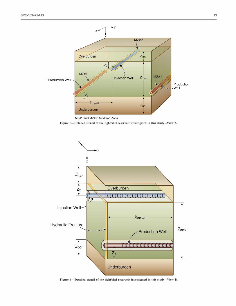
Figure 6—Detailed stencil of the tight/shel reservoir investigated in this study –View B.

Figure 5—Detailed stencil of the tight/shel reservoir investigated in this study –View A.

SPE-169479-MS 13

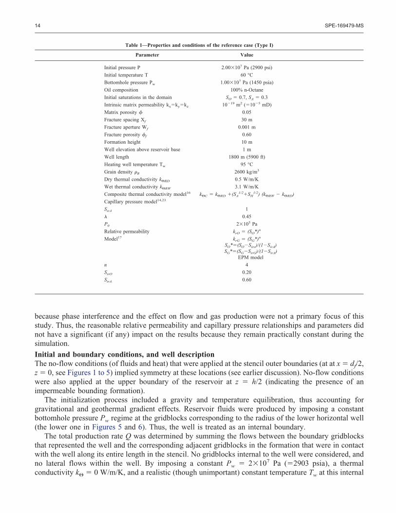
because phase interference and the effect on flow and gas production were not a primary focus of thisstudy. Thus, the reasonable relative permeability and capillary pressure relationships and parameters didnot have a significant (if any) impact on the results because they remain practically constant during thesimulation.

Initial and boundary conditions, and well descriptionThe no-flow conditions (of fluids and heat) that were applied at the stencil outer boundaries (at at x � df/2,z � 0, see Figures 1 to 5) implied symmetry at these locations (see earlier discussion). No-flow conditionswere also applied at the upper boundary of the reservoir at z � h/2 (indicating the presence of animpermeable bounding formation).

The initialization process included a gravity and temperature equilibration, thus accounting forgravitational and geothermal gradient effects. Reservoir fluids were produced by imposing a constantbottomhole pressure Pw regime at the gridblocks corresponding to the radius of the lower horizontal well(the lower one in Figures 5 and 6). Thus, the well is treated as an internal boundary.

The total production rate Q was determined by summing the flows between the boundary gridblocksthat represented the well and the corresponding adjacent gridblocks in the formation that were in contactwith the well along its entire length in the stencil. No gridblocks internal to the well were considered, andno lateral flows within the well. By imposing a constant Pw � 2�107 Pa (�2903 psia), a thermalconductivity k � 0 W/m/K, and a realistic (though unimportant) constant temperature Tw at this internal

Table 1—Properties and conditions of the reference case (Type I)

Parameter Value

Initial pressure P 2.00�107 Pa (2900 psi)

Initial temperature T 60 °C

Bottomhole pressure Pw 1.00�107 Pa (1450 psia)

Oil composition 100% n-Octane

Initial saturations in the domain SO � 0.7, SA � 0.3

Intrinsic matrix permeability kx�ky�kz 10�19 m2 (�10�5 mD)

Matrix porosity � 0.05

Fracture spacing Xf 30 m

Fracture aperture Wf 0.001 m

Fracture porosity �f 0.60

Formation height 10 m

Well elevation above reservoir base 1 m

Well length 1800 m (5900 ft)

Heating well temperature Tw 95 °C

Grain density �R 2600 kg/m3

Dry thermal conductivity kRD 0.5 W/m/K

Wet thermal conductivity kRW 3.1 W/m/K

Composite thermal conductivity model16 kC � kRD �(SA1/2�SH

1/2) (kRW � kRD)

Capillary pressure model14,23

SirA 1

� 0.45

P0 2�105 Pa

Relative permeability krO � (SO*)n

Model17 krG � (SG*)n

SO*�(SO�Siro)/(1�SirA)SG*�(SG�SirG)/(1�SirA)

EPM model

n 4

SirO 0.20

SirA 0.60

14 SPE-169479-MS

boundary, a realistic constant-P condition regime was implemented, while avoiding any non-physicaltemperature distribution in the well vicinity when the simulations were conducted non-isothermally (thelarge advective flows into the gridblocks representing the well from its immediate neighbors eliminatedany unrealistic heat transfer effects that could have resulted from an incorrect k and/or Tw).

Numerical treatment of the fractured subdomainsThe primary (hydraulically-induced) fractures in subdomain S2 as treated as discrete fractures, i.e., theyare described as a porous medium with its own distinct flow properties. This approach allows seamlessinteraction with other fractures and the matrix in the remaining subdomains of the system.

The flow bewteen fractures and matrix in the remaining subdomains is more complex, and is describedby the method of Multiple INteracting Continua (MINC) proposed by Pruess and Narasimhan (1982;1985). In MINC, resolution of these gradients is achieved by appropriate subgridding of the matrix blocks,as shown in Figure 7. The MINC concept is based on the notion that changes in fluid pressures,temperatures, phase compositions, etc., due to the presence of sinks and sources (production and injectionwells) will propagate rapidly through the fracture system, while invading the tight matrix blocks onlyslowly. Therefore, changes in matrix conditions will (locally) be controlled by the distance from thefractures. Fluid and heat flow from the fractures into the matrix blocks, or from the matrix blocks into thefractures, can then be modeled by means of one-dimensional strings of nested grid blocks, as shown inFigure 7.

In general it is not necessary to explicitly consider subgrids in all of the matrix blocks separately.Within a certain reservoir grid block, all fractures will be lumped into continuum # 1, all matrix materialwithin a certain distance from the fractures will be lumped into continuum # 2, matrix material at largerdistance becomes continuum # 3, and so on. Quantitatively, the subgridding defines nested shells that arespecified by means of a set of volume fractions VFj into which the primary porous medium grid blocksare partitioned. The information on fracturing (spacing, number of sets, shape of matrix blocks) requiredfor this is provided by a proximity function which expresses, for a given reservoir domain Vo, the totalfraction of matrix material within a distance l from the fractures. If only two continua are specified (onefor fractures, one for matrix), the MINC approach reduces to the conventional double-porosity method.Full details can be found in Pruess (1983).

Figure 7—Subgridding in the method of “Multiple INteracting Continua” (MINC) (from Pruess et al., 1999).

SPE-169479-MS 15

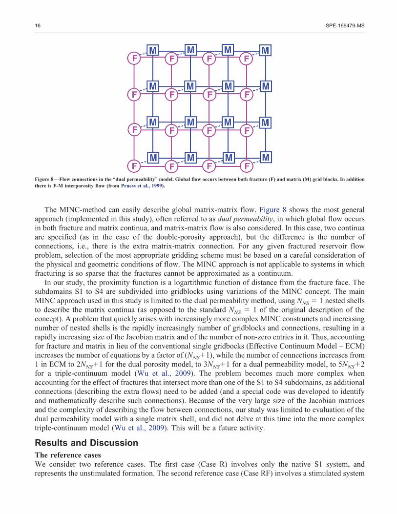
The MINC-method can easily describe global matrix-matrix flow. Figure 8 shows the most generalapproach (implemented in this study), often referred to as dual permeability, in which global flow occursin both fracture and matrix continua, and matrix-matrix flow is also considered. In this case, two continuaare specified (as in the case of the double-porosity approach), but the difference is the number ofconnections, i.e., there is the extra matrix-matrix connection. For any given fractured reservoir flowproblem, selection of the most appropriate gridding scheme must be based on a careful consideration ofthe physical and geometric conditions of flow. The MINC approach is not applicable to systems in whichfracturing is so sparse that the fractures cannot be approximated as a continuum.

In our study, the proximity function is a logartithmic function of distance from the fracture face. Thesubdomains S1 to S4 are subdivided into gridblocks using variations of the MINC concept. The mainMINC approach used in this study is limited to the dual permeability method, using NNS � 1 nested shellsto describe the matrix continua (as opposed to the standard NNS � 1 of the original description of theconcept). A problem that quickly arises with increasingly more complex MINC construncts and increasingnumber of nested shells is the rapidly increasingly number of gridblocks and connections, resulting in arapidly increasing size of the Jacobian matrix and of the number of non-zero entries in it. Thus, accountingfor fracture and matrix in lieu of the conventional single gridbocks (Effective Continuum Model – ECM)increases the number of equations by a factor of (NNS�1), while the number of connections increases from1 in ECM to 2NNS�1 for the dual porosity model, to 3NNS�1 for a dual permeability model, to 5NNS�2for a triple-continuum model (Wu et al., 2009). The problem becomes much more complex whenaccounting for the effect of fractures that intersect more than one of the S1 to S4 subdomains, as additionalconnections (describing the extra flows) need to be added (and a special code was developed to identifyand mathematically describe such connections). Because of the very large size of the Jacobian matricesand the complexity of describing the flow between connections, our study was limited to evaluation of thedual permeability model with a single matrix shell, and did not delve at this time into the more complextriple-continuum model (Wu et al., 2009). This will be a future activity.

Results and DiscussionThe reference casesWe consider two reference cases. The first case (Case R) involves only the native S1 system, andrepresents the unstimulated formation. The second reference case (Case RF) involves a stimulated system

Figure 8—Flow connections in the “dual permeability” model. Global flow occurs between both fracture (F) and matrix (M) grid blocks. In additionthere is F-M interporosity flow (from Pruess et al., 1999).

16 SPE-169479-MS

with hydraulically-induced fractures, i.e., it comprises both S1 and S2 subdomains. The dimensions ofthese two systems are listed in Table 1.

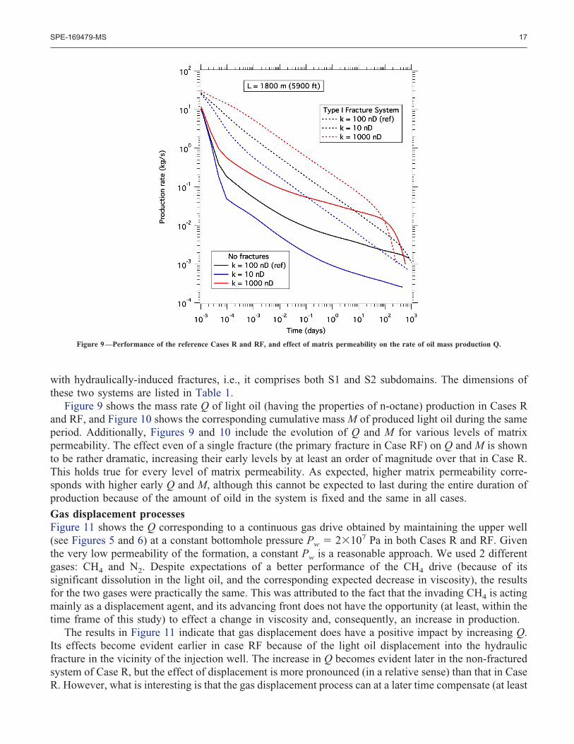
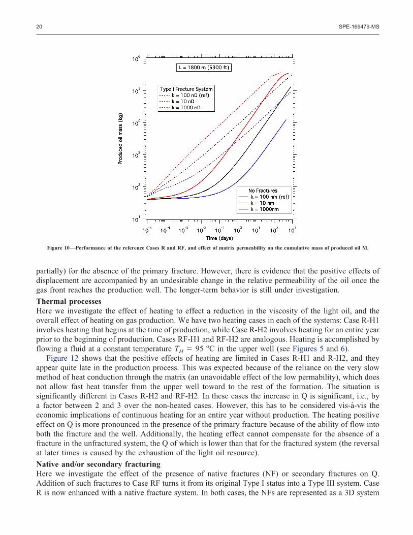
Figure 9 shows the mass rate Q of light oil (having the properties of n-octane) production in Cases Rand RF, and Figure 10 shows the corresponding cumulative mass M of produced light oil during the sameperiod. Additionally, Figures 9 and 10 include the evolution of Q and M for various levels of matrixpermeability. The effect even of a single fracture (the primary fracture in Case RF) on Q and M is shownto be rather dramatic, increasing their early levels by at least an order of magnitude over that in Case R.This holds true for every level of matrix permeability. As expected, higher matrix permeability corre-sponds with higher early Q and M, although this cannot be expected to last during the entire duration ofproduction because of the amount of oild in the system is fixed and the same in all cases.

Gas displacement processesFigure 11 shows the Q corresponding to a continuous gas drive obtained by maintaining the upper well(see Figures 5 and 6) at a constant bottomhole pressure Pw � 2�107 Pa in both Cases R and RF. Giventhe very low permeability of the formation, a constant Pw is a reasonable approach. We used 2 differentgases: CH4 and N2. Despite expectations of a better performance of the CH4 drive (because of itssignificant dissolution in the light oil, and the corresponding expected decrease in viscosity), the resultsfor the two gases were practically the same. This was attributed to the fact that the invading CH4 is actingmainly as a displacement agent, and its advancing front does not have the opportunity (at least, within thetime frame of this study) to effect a change in viscosity and, consequently, an increase in production.

The results in Figure 11 indicate that gas displacement does have a positive impact by increasing Q.Its effects become evident earlier in case RF because of the light oil displacement into the hydraulicfracture in the vicinity of the injection well. The increase in Q becomes evident later in the non-fracturedsystem of Case R, but the effect of displacement is more pronounced (in a relative sense) than that in CaseR. However, what is interesting is that the gas displacement process can at a later time compensate (at least

Figure 9—Performance of the reference Cases R and RF, and effect of matrix permeability on the rate of oil mass production Q.

SPE-169479-MS 17

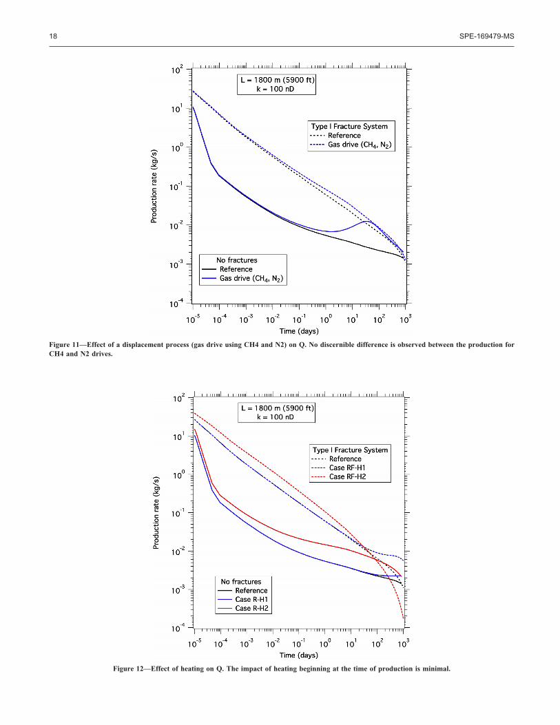
Figure 11—Effect of a displacement process (gas drive using CH4 and N2) on Q. No discernible difference is observed between the production forCH4 and N2 drives.

Figure 12—Effect of heating on Q. The impact of heating beginning at the time of production is minimal.

18 SPE-169479-MS

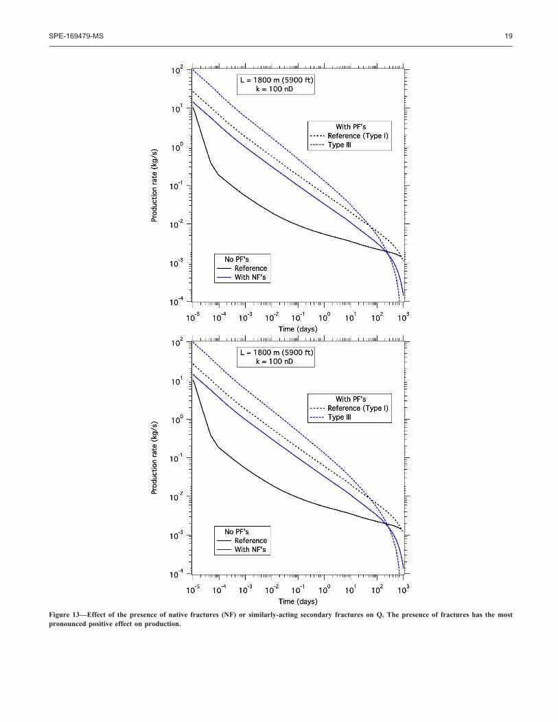
Figure 13—Effect of the presence of native fractures (NF) or similarly-acting secondary fractures on Q. The presence of fractures has the mostpronounced positive effect on production.

SPE-169479-MS 19

partially) for the absence of the primary fracture. However, there is evidence that the positive effects ofdisplacement are accompanied by an undesirable change in the relative permeability of the oil once thegas front reaches the production well. The longer-term behavior is still under investigation.

Thermal processesHere we investigate the effect of heating to effect a reduction in the viscosity of the light oil, and theoverall effect of heating on gas production. We have two heating cases in each of the systems: Case R-H1involves heating that begins at the time of production, while Case R-H2 involves heating for an entire yearprior to the beginning of production. Cases RF-H1 and RF-H2 are analogous. Heating is accomplished byflowing a fluid at a constant temperature TH � 95 oC in the upper well (see Figures 5 and 6).

Figure 12 shows that the positive effects of heating are limited in Cases R-H1 and R-H2, and theyappear quite late in the production process. This was expected because of the reliance on the very slowmethod of heat conduction through the matrix (an unavoidable effect of the low permability), which doesnot allow fast heat transfer from the upper well toward to the rest of the formation. The situation issignificantly different in Cases R-H2 and RF-H2. In these cases the increase in Q is significant, i.e., bya factor between 2 and 3 over the non-heated cases. However, this has to be considered vis-a-vis theeconomic implications of continuous heating for an entire year without production. The heating positiveeffect on Q is more pronounced in the presence of the primary fracture because of the ability of flow intoboth the fracture and the well. Additionally, the heating effect cannot compensate for the absence of afracture in the unfractured system, the Q of which is lower than that for the fractured system (the reversalat later times is caused by the exhaustion of the light oil resource).

Native and/or secondary fracturingHere we investigate the effect of the presence of native fractures (NF) or secondary fractures on Q.Addition of such fractures to Case RF turns it from its original Type I status into a Type III system. CaseR is now enhanced with a native fracture system. In both cases, the NFs are represented as a 3D system

Figure 10—Performance of the reference Cases R and RF, and effect of matrix permeability on the cumulative mass of produced oil M.

20 SPE-169479-MS

with a fracture density of 1 per m, and an aperture of 0.1 mm, and the domain is simulated using the MICconcept. The results in Figure 13 indicate that the addition of the NFs has a dramatic effect on production,which incrases (initially, before the onset of exhaustion of the resource) by several times over thereference Cases R and RF. The impact is more pronounced in Case R.

ConclusionsThe following conclusions can be drawn from this study:

X The presence of fractures (hydraulically-induced or native) is by far the most important factor inincreasing the production of light oil from tight- and shale reservoirs. The importance of thesefractures easily outstrips every other method we investigated (at least within the limited time frameof this study).

X Heating that begins at the time of production appears to have a very limited positive effect onproduction of light oil from tight- and shale reservoirs. Early heating before the onset of productionis quite beneficial, but the economics of heating for a prolonged period (on the order of a year) haveto be considered.

X Gas drives have a positive impact, but this is not very pronounced and appears later in theproduction process. The benefits of viscosity reduction through CH4 dissolution in the light oil (vs.N2-drive) are not evident during the time frame of this study, possibly because the advancing CH4

front acts only as a displacement agent without sufficient penetration into the light oil.

AcknowledgmentsThe authors wish to thank the Crisman Institute for Petroleum Research at Texas A&M University forpartial support of this work.

Nomenclature

A � surface area, surface area of subdomain n, m2

b � Klinkenberg parameter, PaBgi � Langmuir constant of natural gas component gi, 1/Pact � Total compressibility, 1/Pa

� Multicomponent molecular diffusion coefficient of component � in the gas phase, m2 s�1

� Dispersion tensor of component � in phase �f� � Radiance emittance factor, dimensionlessF� � Flux vector of component �, kg m�2s�1,g � Gravitational acceleration vector, m s�2

h � Specific enthalpy (component), J/kgH � Specific enthalpy (phase), J/kgHgi � Temperature-dependent Henry’s factor describing the solution of gas gi (i � 1, . . ., NG)

in H2O, Pa� Diffusive mass flux of component � in the phase �, kg m�2 s�1

k � Intrinsic permeability, m2

kr� � Relative permeability of phase �, dimensionlessKn � Knudsen diffusion number, dimensionlessmL � Langmuir mass, kg/Pa (equation (3))M � Cumulative mass of produced oil, kgMW � Molecular weight of a component �, kg/moln � Inward unit normal vectorNG � Number of components of natural gas

SPE-169479-MS 21

p � Pressure, PapL � Langmuir pressure, Pa (equation (3))Y � Langmuir storage, kg/kgq � Mass or heat rate of a source or sink, kg/s or Wsf � Fracture spacing, mS � phase saturationk � Matrix permeability, m2

pi � Initial reservoir pressure, PaPw � Well bottomhole pressure, Pat � Time, daysT � Temperature, K or °Cu � Specific internal energy (component), J/kgU � Specific internal energy (phase), J/kgv� � Darcy velocity vector of phase �v� � Length of vector v�, m/sV, Vn � volume, volume of subdomain n, m3

� Dispersive mass flux of component � in phase � (�A,O,C), kg m�2 s�1

� Mass fraction of component � in phase �

Greek Symbols

� � From equation (18)� Transverse and longitudinal dispersivities of component � in phase �, m

�T � Thermal expansivity of the porous medium, 1/K�P � Medium pore compressibility, 1/Pa��T � Turbulence correction factor, dimensionless (equation (20)) � Permeability reduction factor, dimensionless (equation (26))�n � Surface area, surface area of subdomain n, m2

� � Mean free path of a gas, m� � Porosity� � Viscosity, Pa.s� � density, kg m�3

�0 � Stefan-Boltzmann constant � 5.6687 � 10�8 J m�2 K�4

� � Tortuosity of phase �, dimensionless

Subscripts and Superscripts

� � Denotes a phase (� � G, A, O, C)� � Heat (treated as a pseudo-component)�RD � Denotes “dry” (gas-saturated) thermal consuctivity�RW � Denotes “wet” (liquid-saturated) thermal consuctivity� � Indicates a component � � gi (i � 1, . . ., NG), oj (j � 1,2), w0 � Denotes initial stateA � Denotes aqueous phasecGW � Gas-water capillary pressureC � Denotes liquid CO2 phasegi � Denotes a component of the natural gas (i � 1, . . ., NG)G � Gas phaseoj � Denotes an oil component of the organic phase (i � 1, . . ., NG)

22 SPE-169479-MS

O � Organic phaser� � Denotes an oil component of the organic phase (i � 1, . . ., NG)R � Rockw � Denotes water component (e.g., � � w) or well (e.g., Pw)

ReferencesAnderson, D.M., Nobakht, M., Moghadam, S. and Mattar, L. 2010. Analysis of Production Data from

Fractured Shale Gas Well. Paper SPE 131787 presented at the SPE Unconventional Gas Conference heldin Pittsburgh, Pennsylvania, 23-25 February 2010.

Aguilera, R. 2010. Flow Units: From Conventional to Tight Gas to Shale Gas Reservoirs. Paper SPEpresented at the Trinidad and Tobago Energy Resources Converence held in Port of Spain, Trinidad,27-30 June 2010.

Amini, S., Ilk, D., and Blasingame, T.A. 2007. Evaluation of the Elliptical Flow Period for Hydrau-lically-Fractured Wells in Tight Gas Sands — Theoretical Aspects and Practical Considerations. PaperSPE 106308 presented at the SPE Hydraulic Fracturing Technology Conference, College Station, Texas,29-31 January.

Brown, M., Ozkan, E., Raghavan, R., Kazemi, H. Practical Solutions for Pressure Transient Responsesof Fractured Horizontal Wells in Unconventional Reservoirs. Paper SPE 125043 presented at the 2009SPE Annual Technical Conference and Exhibition held in New Orleans, Louisiana, USA, 4-7 October2009.

Bowker, K.A. 2007. Barnett Shale Gas Production, Fort Worth Basin: Issues and Discussion. AAPGBulletin 91 (4): 523–533.

Bumb, A.C. and McKee, C.R. 1988. Gas–Well Testing in the Presence of Desorption for CoalbedMethane and Devonian Shale. SPE Formation Evaluation (March 1988): 179–185. SPE-15227-PA.

Carlson, E.S. and Mercer, J.C. 1991. Devonian Shale Gas Production: Mechanisms and SimpleModels. JPT (April 1991): 476–482. SPE-19311-PA.

Cinco-Ley, H. and Samaniego, F. 1982. Pressure Transient Analysis for Naturally Fractured Reser-voirs. Paper SPE 11026 presented at the SPE Annual Technical Conference and Exhibition, New Orleans,Louisiana, 26–29 September.

Crafton, J.W. 2010. Flowback Performance in Intensely Naturally Fractured Shale Gas Reservoirs.Paper SPE 131785 presented at the SPE Unconventional Gas Conference held in Pittsburgh, Pennsylva-nia, USA, 23-25 February 2010.

Currie, S.M., Ilk, D. and Blasingame, T.A. 2010. Continuous Estimation of Ultimate Recovery. PaperSPE presented at the SPE Unconventional Gas Conference held in Pittsburgh, Pennsylvania, USA, 23-25February 2010.

Curtis, J.B. 2002. Fractured Shale-Gas Systems. AAPG Bulletin 86 (11): 1921–1938.Cox, D.O., Kuuskraa, V.A., and Hansen, J.T. 1996. Advanced Type Curve Analysis for Low

Permeability Gas Reservoirs. Paper SPE 35595 presented at the Gas Technology Conference, Calgary,Alberta, 28 April–1 May.

De Swaan, A.O. 1976. Analytic Solutions for Determining Naturally Fractured Reservoir Propertiesby Well Testing. Society of Petroleum Engineers Journal (June 1976): 117–122. SPE-5346-PA.

Dougherty, E.L. and Chang, J. 2010. A Methodology to Quickly Estimate the Probably Value of ShaleGas Well. Paper SPE 134005 presented at the SPE Western Regional Metting held in Anaheim,California, USA, 27-29 May 2010.

Du, C.M., Zhang, X., Lang, Z., Gu, H., Hay, B., Tushingham, K. and Ma, Y.Z. 2010. ModelingHydraulic Fracturing Induced Fracture Networks in Shale Gas Reservoirs as a Dual Porosity System.Paper SPE 132180 presented at the CPS/SPE International Oil & Gas Conference and Exhibition in Chinaheld in Beijing, China, 8-10 June 2010.

SPE-169479-MS 23

Falta, R., Pruess, K., Finsterle, S., and Battistelli, A., 1995. T2VOC User’s Guide, Lawrence BerkeleyLaboratory Report LBL-36400, Berkeley, CA.

Florence, F.A., Rushing, J.A., Newsham, K.E., and Blasingame, T.A. 2007. Improved PermeabilityPrediction Relations for Low- Permeability Sands. SPE paper 107594, SPE Rocky Mountain Oil & GasTechnology Symposium, Denver, Colorado, 16-18 April.

Frantz, Jr., J.H., Williamson, J.R., Sawyer, W.K., Johnston, D., Waters, G., Moore, L.P., MacDonald,R.J., Pearcy, M., Ganpule, S.V., and March, K.S. 2005. Evaluating Barnett Shale Production PerformanceUsing an Integrated Approach. Paper SPE 96917 presented at the SPE Annual Technical Conference andExhibition, Dallas, Texas, 9–12 October.

Freeman, C.M., Moridis, G.J., and Blasingame, T.A. 2009a. A numerical study of microscale flowbehavior in tight gas and shale gas reservoir systems. Proceedings, 2010 TOUGH Symposium, Berkeley,CA, 14-16 September.

Freeman, C.M., Moridis, G.J., Ilk, D., and Blasingame, T.A. 2009b. A numerical study of tight gas andshale gas reservoir systems. SPE paper 124961, SPE Annual Technical Conference and Exhibition, NewOrleans, Louisiana, 4-9 October.

Freeman, C.M., Moridis, G., Ilk, D. and Blasingame, T.A. 2010. A Numerical Study of Transport andStorage Effects for Tight Gas and Shale Gas Reservoir Systems. Paper SPE 131583 presented at the SPEInternational Oil & Gas Conference and Exhibition held in Beijing, China, 8-10 June 2010.

Gao, C., Lee, J.W., Spivey, J.P., and Semmelbeck, M.E. 1994. Modeling Multilayer Gas ReservoirsIncluding Sorption Effects. SPE paper 29173 presented at the SPE Eastern Regional Conference &Exhibition, Charleston, West Virginia, 8-10 November.

Hale, B.W. 1986. Analysis of Tight Gas Well Production Histories in the Rocky Mountains. SPEProduction Engineering (July 1986): 310–322. SPE-11639-PA.

Hazlett, W.G., Lee, W.J., Narahara, G.M., and Gatens, III, J.M. 1986. Production Data Analysis TypeCurves for Devonian Shales. Paper SPE 15934 presented at the SPE Eastern Regional Meeting, Colum-bus, Ohio, 12–14 November.

Ilk, D., Rushing, J.A., Perego, A.D., and Blasingame, T.A. 2008. Exponential vs. Hyperbolic Declinein Tight Gas Sands — Understanding the Origin and Implications for Reserve Estimates Using Arps’Decline Curves. Paper SPE 116731 presented at the SPE Annual Technical Conference and Exhibition,Denver, Colorado, 21-24 September.

Ilk, D., Anderson, D.M., Stotts, G.W.J., Mattar, L., Blasingame, T.A. 2010. Production-Data Analysis– Challenges, Pitfalls, Diagnostics. SPE Reservoir Evaluation & Engineering (Jun. 2010): 534–552.SPE-102084-PA.

Javadpour, F., Fisher, D., and Unsworth, M. 2007. Nanoscale Gas Flow in Shale Gas Sediments. JCPT46 (10): 55–61.

Karniadakis, G.E., and Beskok, A. 2001: “Microflows: Fundamentals and Simulation”, Springer.Klinkenberg, L.J. 1941. “The Permeability of Porous Media to Liquid and Gases,” API Drilling and

Production Practice, 200–213.Kucuk, F. and Sawyer, K. 1980. Transient Flow in Naturally Fractured Reservoirs and its Application

to Devonian Gas Shales. Paper SPE 9397 presented at the SPE Annual Technical Conference andExhibition, Dallas, Texas, 21–24 September.

Lewis, A.M. and Hughes, R.G. 2008. Production Data Analysis of Shale Gas Reservoirs. Paper SPE116688 presented at the SPE Annual Technical Conference and Exhibition, Denver, Colorado, 21–24September.

Maley, S. 1985. The Use of Conventional Decline Curve Analysis in Tight Gas Well Applications.Paper SPE 13898 presented at the SPE/DOE Low Permeability Gas Reservoirs, Denver, Colorado, 19–22May.

Mattar, L., Gault, B., Morad, K., Clarkson, C.R., Freeman, C.M., Ilk, D., and Blasingame, T.A. 2008.

24 SPE-169479-MS

Production Analysis and Forecasting of Shale Gas Reservoirs: Case History-Based Approach. Paper SPE119897 presented at the SPE Shale Gas Production Conference, Fort Worth, Texas, 16–18 November.

McCain, W.D., Spivey, J.P., and Lenn, C.P. 2011: “Microflows: Fundamentals and Simulation”,PennWell, Tulsa, Oklahoma.

Medeiros, F., Ozkan, E., and Beskok, A. 2001: “Petroleum Reservoir Fluid Property Correlations”,Springer.

Medeiros, F., Kurtoglu, B., Ozkan, E., and Kazemi, H. 2007. Analysis of Production Data fromHydraulically Fractured Horizontal Wells in Tight, Heterogeneous Formations. Paper SPE 110848presented at the SPE Annual Technical Conference and Exhibition, Anaheim, California, 11-14 Novem-ber.

Millington, R.J., and Quirk, J.P. 1961. Permeability of porous solids. Trans. Faraday Soc. 57:1200–1207.

Moridis, G.J., Kowalsky, M.B., Pruess, K., 2008c. TOUGH�HYDRATE v1.0 User’s Manual: A Codefor the Simulation of System Behavior in Hydrate-Bearing Geologic Media, Report LBNL-00149E,Lawrence Berkeley National Laboratory, Berkeley, CA.

Moridis, G.J., T.A. Blasingame, and C.M. Freeman. Analysis of Mechanisms of Flow in FracturedTight-Gas and Shale-Gas Reservoirs, Paper SPE 139250, SPE Latin American & Caribbean PetroleumEngineering Conference, Lima, Peru, 1–3 December 2010.

Najurieta, H.L. 1980. A Theory for Pressure Transient Analysis in Naturally Fractured Reservoirs.JPT (June 1980): 1241–1250. SPE-6017-PA

Neal, D.B. and Mian, M.A. 1989. Early-Time Gas Production Forecasting Technique ImprovesReserves and Reservoir Description. SPE Formation Evaluation (March 1989): 25–32. SPE-15432-PA.

Nobakht, M., Mattar, L., Moghadam, S. and Anderson, D.M. 2010. Simplified Yet Rigorous Fore-casting of Tight/Shale Gas Production in Linear Flow. Paper SPE 133615 presented at the SPE WesternRegional Meeting held in Anaheim, California, USA, 27-29 May 2010.

Passey, Q.R., Bohacs, K.M., Esch, W.L., Klimentidis, R. and Sinha, S. 2010. From Oil-Prone SourceRock to Gas-Producing Shale Reservoir - Geological and Petrophysical Characterization of Unconven-tional Shale-Gas Reservoirs. Paper SPE 131350 presented at the CPS/SPE International Oil & GasConference and Exhibition in China held in Beijing, China, 8-10 June 2010.

Poling, B.E., Prausnitz, J.M., and O’Connel, J.P. 2001: “The Properties of Gases and Liquids”, 5thEdition, McGraw-Hill, New York, New York.

Pollastro, R.M. 2007. Total Petroleum System Assessment of Undiscovered Resources in the GiantBarnett Shale Continuous (Unconventional) Gas Accumulation, Fort Worth Basin, Texas. AAPG Bulletin91 (4): 551–578.

Pruess, K., 1983. GMINC - A Mesh Generator for Flow Simulations in Fractured Reservoirs,Lawrence Berkeley Laboratory Report LBL-15227, Berkeley, CA.

Pruess, K., Narasimhan, T.N., 1982. On Fluid Reserves and the Production of Superheated Steam fromFractured, Vapor-Dominated Geothermal Reservoirs, J. Geophys. Res., 87(B11), 9329–9339.

Pruess, K., Narasimhan, T.N., 1985. A Practical Method for Modeling Fluid and Heat Flow inFractured Porous Media, Soc. Pet. Eng. J., 25(1), 14–26.

Pruess, K., C. Oldenburg, and G. Moridis, 1999, TOUGH2 User’s Guide – Version 2.0, LawrenceBerkeley Laboratory Report LBL-43134, Berkeley, CA.

Serra, K., Reynolds, A.C., and Raghavan, R. 1983. New Pressure Transient Analysis Methods forNaturally Fractured Reservoirs. JPT (Dec. 1983): 2271–2283. SPE-10780-PA.

Sinha, M.K. and Furlong, K.D. 1979. Gas Well Deliverability Prediction — For HydraulicallyFractured (Vertical) Wells in Tight Reservoirs. Paper SPE 7948 presented at the SPE Symposium onLow-Permeability Gas Reservoirs, Denver, Colorado, 20–22 May.

Thompson, J.K. 1981. Use of Constant Pressure, Finite Capacity Type Curves for Performance

SPE-169479-MS 25

Prediction of Fractured Wells in Low– Permeability Reservoirs. Paper SPE 9839 presented at theSPE/DOE Low Permeability Symposium, Denver, Colorado, 27–29 May.

van Kruysdijk, C.P.J.W. and Dullaert, G.M. 1989. A Boundary Element Solution of the TransientPressure Response of Multiple Fractured Horizontal Wells. Paper presented at the 2nd EuropeanConference on the Mathematics of Oil Recovery, Cambridge, England.

Warren, J.E, Root, P.J., 1963. The Behavior of Naturally Fractured Reservoirs, Soc. Pet. Eng. J.,Transactions, AIME, 228, 245–255.

Wu, Y.-S., Moridis, G., Bai B., Zhang, K., 2009, A multi-continuum model for gas production in tightfractured reservoirs, SPE paper 118944, SPE Hydraulic Fracturing Technology Conference, 19-21January 2009, The Woodlands, Texas.

Zhang, K., Moridis, G.J., 2008. A Domain Decomposition Approach for Large-Scale Simulations ofCoupled Processes in Hydrate-Bearing Geologic Media, Proceedings, 6th International Conference onGas Hydrates, Vancouver, British Columbia, Canada, July 6-10.

Zhang, X., Du, C., Deimbacher, F., Crick, M. and Harikesavanallur, A. 2009. Sensitivity Studies ofHorizontal Wells with Hydraulic Fractures in Shale Gas Reservoirs. Paper SPE IPTC 13338 presented atthe International Petroleum Technology Conference held in Doha, Qater, 7-9 December.

Zuber, M.D., Frantz, Jr., J.H., and Gattens, III, J.M. 1994. Reservoir Characterization and ProductionForecasting for Antrim Shale Wells: An Integrated Reservoir Analysis Methodology. Paper SPE 28606presented at the SPE Annual Technical Conference and Exhibition, New Orleans, Louisiana, 25–28September.

26 SPE-169479-MS