Embed Size (px)
Citation preview

Speaker Clustering in Speech Recognition
Olga Grebenskaya 04.03.2005 University of Joensuu Department of Computer Science Master’s Thesis
ii
TABLE OF CONTENTS
1 INTRODUCTION.......................................................................................................................1
1.1 Automatic speech recognition system (ASR) .........................................................................1
1.2 ASR classification.....................................................................................................................1
1.3 General ASR structure..............................................................................................................2
1.4 Structure of the theses...............................................................................................................3
2 SPEECH RECOGNITION BASICS........................................................................................4
2.1 Speech........................................................................................................................................4
2.2 Phonology basics.......................................................................................................................6
2.3 Probabilistic speech model.......................................................................................................8
3 FEATURE EXTRACTION.....................................................................................................11
3.1 Pre-emphasis ...........................................................................................................................11
3.2 Windowing ..............................................................................................................................12
3.3 Linear predictive coding (LPC) .............................................................................................13
3.4 Mel-frequency cepstrum (MFCC) .........................................................................................14
3.5 Dynamic characteristics..........................................................................................................15
4 HIDDEN MARKOV MODELS..............................................................................................17
4.1 Fundamentals of HMMs.........................................................................................................17
4.2 Recognition with HMM..........................................................................................................19
4.3 Viterbi decoding......................................................................................................................22
4.4 HMM training .........................................................................................................................24
4.5 Context dependent modeling..................................................................................................29
5 USING SPEAKER INFORMATION IN SPEECH RECOGNITION.............................32
5.1 Speaker adaptation..................................................................................................................32
iii
5.2 Speaker clustering...................................................................................................................35
6 SPEECH RECOGNITION SYSTEM BUILDING .............................................................42
6.1 HTK description......................................................................................................................42
6.2 Training ...................................................................................................................................42
6.3 Testing .....................................................................................................................................47
7 EXPERIMENTS .......................................................................................................................50
7.1 Test setup.................................................................................................................................50
7.2 Results......................................................................................................................................51
7.3 Discussion................................................................................................................................52
8 CONCLUSIONS .......................................................................................................................54
REFERENCES ..................................................................................................................................55
APPENDIX A.....................................................................................................................................59
APPENDIX B.....................................................................................................................................61
APPENDIX C.....................................................................................................................................62

iv
List of Figures
Figure 1.1: Classification of ASR systems. ....................................................................................1 Figure 1.2: Basic ASR blocks..........................................................................................................2 Figure 2.1: Human speech production apparatus. ..........................................................................4 Figure 2.2: Glottis oscillation. .........................................................................................................5 Figure 2.3: Source-filter model of speech production. Examples are given for two case of F0: 100 Hz (upper picture) and 200 Hz. ................................................................................................6 Figure 2.4: Spectrogram (left) and a waveform for phoneme /ih/.................................................7 Figure 2.5: English consonants classification based of the manner of articulation. [±V] denotes voced/unvoised characteristics. .......................................................................................................8 Figure 2.6: Probabilistic speech recognition model. ....................................................................10 Figure 3.1: Unprocessed (left) and pre-emphasized (right) signals. ...........................................11 Figure 3.2: Short-time speech analysis. ........................................................................................12 Figure 3.3: LPC and LPCC computation flowchart. ....................................................................14 Figure 3.4: Critical band filters used in MFCC computation and their outputs (s1 s2…sM). .....14 Figure 4.1: “HMM in action”. .......................................................................................................17 Figure 4.2: Isolated word recognition with HMMs λ2, λ2… λK...................................................19 Figure 4.3: An example of 3-state HMM for modeling. ..............................................................20 Figure 4.4: Forward algorithm proceeding. ..................................................................................21 Figure 4.5: Backward algorithm proceeding. ...............................................................................22 Figure 4.6: Viterbi algorithm proceeding. The resulting state sequence is 1-2-3. .....................24 Figure 4.7: Segmental k-means algorithm example. ....................................................................26 Figure 4.8: The tree-based state clustering algorithm flowchart. ................................................30 Figure 4.9: Tree-based state clustering example for the central state of ‘ao’ triphones. ...........31 Figure 5.1: MLLR adaptation for means. .....................................................................................34 Figure 5.2: Regression class tree for MLLR. Wi denotes the transformation matrix shared by the specific class. ............................................................................................................................34 Figure 5.3: Speaker clustering utilized in speech recognition.....................................................35 Figure 5.4: Flowchart of the proposed metaclustering algorithm. ..............................................39 Figure 5.5: Steps involved in metaclustering. Step 3 and 4 represent one iteration of the algorithm while the first two steps are initialization. ...................................................................39 Figure 5.6: Pseudocode for calculations of the distance between two codebooks.....................40 Figure 5.7: Involving metaclustering in training process. ...........................................................40 Figure 6.1: The main parts of HTK: training and recognition tools............................................42 Figure 6.2: Steps of ASR building using HTK.............................................................................43 Figure 6.3: HMM with three emitting states used for monophones............................................44 Figure 6.4: Creating a composite HMM for embedded training. ................................................44 Figure 6.5: Silence (‘sil’) and short-pause (‘sp’) models with tied states and added transitions..........................................................................................................................................................45 Figure 6.6: The main steps in triphones-based speech recognition system training. .................47 Figure 6.7: The testing process outline. ........................................................................................47 Figure 6.8: Word network example for words ‘yes’ and ‘no’. ....................................................48 Figure 6.9: Expanded network where each word is substituted by the corresponding phone sequence. Word-end node is denoted as WE................................................................................48 Figure 6.10: The last step in network compilation. Each node is replaced by corresponding HMM...............................................................................................................................................49 Figure 6.11: An example of possible errors during recognition. ‘S’ denotes substitution, ‘D’ deletion and ‘I’ insertion................................................................................................................49

v
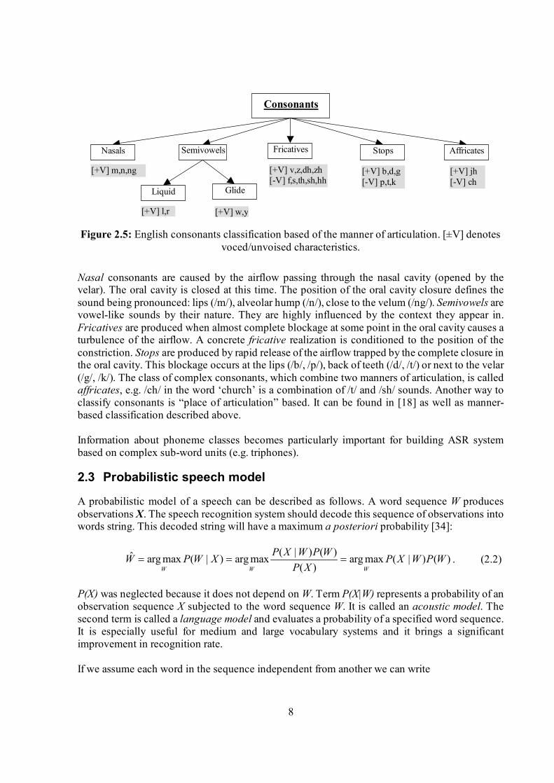
Figure 7.1: Recognition accuracy for varying number of speaker clusters (speaker codebook size = 64).........................................................................................................................................51 Figure 7.2: Recognition accuracy for varying codebook size (number of speaker clusters = 4)..........................................................................................................................................................52 Figure 7.3: Metaclustering tested on 2D artificial data for the case of two clusters..................53 Figure 7.4: Male/female division in a case of 4 clusters and codebook size of 8. .....................53 Figure C.1: Speaker recognition system schema..........................................................................62 Figure C.2: VQ-based speaker identification process..................................................................63

vi
List of Tables
Table 4.1: Within- and cross-word expansion example for the first two words in the sentence “The emperor had a mean temper”................................................................................................29 Table 7.1: Speakers and sentences of the testing and training sets. ............................................50 Table 7.2: Recognition accuracy for varying number of speaker clusters..................................51 Table 7.3: Recognition accuracy for varying codebook size (number of speaker clusters = 4)..........................................................................................................................................................52 Table B.1: Phone mapping from 45 to 39-phone set....................................................................61

vii
Abstract
Automatic speech recognition along with speaker recognition and text to speech conversion is a fundamental task in speech processing. Natural speech recognition is a difficult and challenging research area. Since the latest 1970s, the performance of speech recognition engines has significantly increased due to involving stochastic approaches for acoustic modeling. However, there is still a wide gap to fill in for building high performance speech recognition systems. For example, the task of spontaneous speech recognition is still far from to be solved. One of the latest tendencies in improving accuracy is incorporation of speaker information in speech recognition. This includes speaker adaptation, normalization and clustering techniques as well as their combinations. Achievements in speaker recognition research show another way of incorporating information of speaker individuality in speech recognition. Speaker recognition techniques are computational effective and make a reliable decision based on a limited data (just few seconds of speech). This fact can be used for fast speaker adaptation. This thesis presents clustering algorithm based on speaker models obtained using vector quantization (VQ) method. Such speaker representation is simple and provides fast algorithms for speaker recognition. The idea of the method is to group all speakers into clusters based on their models. Finding clusters of similar speakers on the training stage and treating clusters’ speech material as coming from the same speaker we can create separated sets of models for speech recognition. During recognition, speech from an unknown speaker is used to determine the closest cluster and speech recognition is done on the model set obtained for this cluster. There is a number of different ways to perform speaker grouping. Some of them are outlined in the current work. The topic studied in this thesis explores knowledge from different parts of digital signal processing, statistics and phonetics. First, we discuss speech recognition basics, then consider possible ways of taking advantages of speaker information and finally present the results of the speech recognition with involved speaker clustering. The experiments of speaker clustering were performed on TIMIT database. The best improvement obtained was 6.8% relative word error reduction compared to the baseline results. Key Words: speech recognition, speaker recognition, clustering, speaker adaptation, Hidden Markov Models.

viii
Acknowledgments
I would like to thank my supervisor Pasi Fränti for his guidance and comments during my work on the thesis. I wish to express gratitude to Tomi Kinnunen for his help, knowledge, ideas he shared with me, for his deep interest to speech technology. I would also like acknowledge Juhani Saastamoinen for his HTK advices. My friends, my special thanks for understanding and moral support go to you! Finally, I appreciate my parents for their love, patience and support in all aspects.

1
1 INTRODUCTION
1.1 Automatic speech recognition system (ASR)
Automatic speech recognition (ASR) is a process of interpreting a human’s speech by a computer. It is a wide term and it involves a number of technologies and research areas like signal processing and statistics. A closer related area is speaker recognition, in which the task is to recognize/verify a person’s identity. A wide range of possible applications of ASR includes:
• Dictation applications. • Interactive voice response systems. Such applications allow to free people from a routine
job of talking to the clients answering to simple and often arisen questions. It provides an interactive customer self-service.
• Command and control systems. Provides a natural way of interacting to computer or other device (i.e. mobile phone). Saying something like “File”, “Save” lets the users to use their voices as a “third hand”. This idea can be extended to domestic applications like “intelligent flat”. One just utters commands such as “turn on/off the light/music”. Such applications require some action after the command is recognized.
• Wearables. It is natural to use speech because of limited input possibilities. • Applications for people with typing or hearing difficulties. Speech recognition solutions
can help them to write texts or convert a caller’s speech to text. • Combination of speech and speaker recognition applications for security needs.
1.2 ASR classification
Depending on the chosen criterion ASR systems can be classified as it is shown in Figure 1.1.
Figure 1.1: Classification of ASR systems.
ASR
Speaker mode Vocabulary size Speaking style Speech mode
Isolated utterances
Continuous speech
Speaker independent
Speaker dependent
Speaker adaptive
Small
Medium
Large
Dictation
Spontaneous

2
Speech mode An isolated utterances recognition task requires marking beginning and end of every utterance. User is supposed to make pauses to denote a word (or phrase) to be recognized. On the other hand, continuous speech recognition allows uttering normal phrases used in everyday life. This is very difficult task for recognizers since there are no clear word boundaries available. But such systems are on the target of ASR market because of their possible wide applications. Speaker mode Speaker independent (SI) systems are meant to recognize speech regardless who is actually speaking. They are supposed to be good enough for any possible speaker. In the opposite to them speaker dependent (SD) systems aim to fit an individual speaker better than others and hence perform for him/her better in comparison to SI case. But SI systems meet industrial requirements much more often. Speaker adaptive (SA) case can be thought as a “bridge” between these two ASR types. Adaptation is an approach to bring SI performance close to SD one based on acoustic information from the user who is currently using the system. Vocabulary size Every ASR system uses vocabulary (or lexicon). The vocabulary is considered small if it contains tens of words, medium if it contains hundreds, and large if it consists of thousands of words. The vocabulary content and size are highly dependent on the task it is meant for. For example, a simple digit recognizer requires ten words only while a dictation task cannot work without large dictionary. Speaking style Dictation is a read speech and it is the most common task for nowadays speech recognition systems. Spontaneous speech recognition systems should handle different features of a common speech like stumbling, “em”- and “ah”-like words.
1.3 General ASR structure
The main building blocks of a typical ASR are depicted in Figure 1.2.
Figure 1.2: Basic ASR blocks.
The signal processing module aims to represent a speech signal as a set of vectors called feature vectors. It provides all signal processing steps necessary to obtain those features like digitizing
Signal processing
Speech
Recognition engine Acoustic models
Language models
Adaptation

3
the speech signal, pre-emphasizing, framing etc. The recognition engine decodes these features using acoustic and language models. The former represents knowledge about acoustic realization of a single recognition unit. The latter represents knowledge of what word sequences are likely to appear in the speech. Acoustic models are trained using a big amount of data came from different speakers and probably from different environments. These models are supposed to be well enough for any speaker. Adaptation module adjusts acoustic models so that they represent current testing conditions and speaker better. Although Figure 1.2 does not show the connections between language models and adaptation blocks, it is possible to adapt them as well. However, language model adaptation is out of the scope of this thesis.
1.4 Structure of the theses
The thesis is organized as follows. In the Section 2 the speech recognition basics are given containing phonetics and speech production issues. Section 3 gives an overview of speech processing techniques. Acoustic modeling with Hidden Markov Models is discussed in Section 4. Ways of incorporating speaker information into speech recognition process are discussed in Section 5. Section 6 is devoted to issues of speech recognition system building and Section 7 discusses recognition results of applying speaker clustering to speech recognition. Final conclusions are given in Section 8.

4
2 SPEECH RECOGNITION BASICS
2.1 Speech
Speech can be defined as a process of creating vocal sounds, which form words to express ideas, thoughts etc. These vocal sounds are produced by the human’s speech production apparatus. All the apparatus parts (see Figure 2.1) contribute to the speech production process by changing their shapes, lengths and interacting with each other. The main voice characteristics such as pitch, loudness, and timbre are the result of it. Different sounds can be classified according to the articulators’ positions and analyzed using their spectrograms.
2.1.1 Speech production
Figure 2.1: Human speech production apparatus.
The speech production process proceeds as follows. Air, expelled from the lungs reaches the larynx (or vocal cords). They form a V-like opening, which is called the glottis. Larynx separates the trachea from the vocal tract and plays an important role in speech production. It is responsible for the type of the sound produced (voiced/unvoiced) and can be in different stages:
• Vibration: the vocal cords are held close to each other and open/close periodically producing series of puffs (voiced consonants like /z/, /v/ and vowels)
• Completely open: no vibration, the cords are apart from each other forming a "V" shaped opening (unvoiced sounds like /s/, /f/)

5
• An intermediate position between closed and opened (whisper). In the oscillation mode, the frequency of vibrations is called the fundamental frequency (or pitch) and commonly denoted as F0. Its average value is about 120 Hz, 220 Hz and 330 Hz for males, females and children respectively [21]. The vibration process is shown in Figure 2.2. Periods of completely closed vocal cords (zero amplitude) alternate with opened ones.
Figure 2.2: Glottis oscillation.
Next, the air flow passes through the vocal tract. It consists of the pharynx (the throat cavity), the velum (or soft palate), and the oral and nasal cavities. The shape of the nasal cavity is fixed while the oral cavity’s characteristics can vary depending on sounds being pronounced. The vocal tract is composed of different articulators that change the length and a shape of the vocal tract. These articulators are:
• Pharynx: connects the larynx and the oral cavity • Velum: closes or opens the nasal cavity for pronunciation of such sounds as /m/ and /n/ • Tongue: the most flexible articulator. Its movements in different direction allow to change
the oral cavity shape. For example, pronouncing a sound /s/ a tongue moves forward creating a narrow area with a hard palate while /a/ sound requires an open oral cavity exit so the tongue moves down
• Teeth: used for pronunciation of many sounds while contacting with a tongue • Lips: for some consonants (/p/, /m/ etc.) lips are completely closed while for vowels they
can be rounded (/o/) or spread (/i/) • Hard palate: a bony roof of the mouth. It separates the mouth from the nasal cavity and
allows producing some consonants • Alveolar ridge: is placed between top teeth and hard palate. With a tongue contributes in
producing such sounds as /d/ and /t/. The vocal tract can be thought as a tube (or a concatenation of tubes) of varying cross-sectional area. One end is closed (larynx) and the other one is opened (lips). Acoustic theory predicts that the transfer function of such tube can be described in terms of the natural frequencies (resonances). These frequencies are called the formants and they pass the most part of the acoustic energy. The first three formants (<3500 Hz) play the most significant role in vowel recognition. It will be explained further in the section 2.2 while considering consonants and vowels features.
2.1.2 Source-filter model
A useful for speech analysis way of describing a vocal tract is a source-filter model [18]. The speech production process is thought as a sound source (glottal air flow) passing through the

6
filter (vocal tract). The filter shapes the source spectra as it is illustrated by the Figure 2.3. This example is given for the neutral vowel /ə/ (“bird”) [15]:
Figure 2.3: Source-filter model of speech production. Examples are given for two case of F0:
100 Hz (upper picture) and 200 Hz (bottom picture). It follows from the filter transfer function (pictures in the middle) that the vocal tract has first three formants equal to 500 Hz, 1500 Hz and 2500 Hz. Actually these values can be calculated analytically using the following formula [14]:
L
cnFn 4)12( −= , (2.1)
where L is a vocal tract length, n is a formant number and c is a velocity of sound. As it is seen in the Figure 2.3 the final spectrum is formed by two components: source, or fast-varying part, and filter, or slow-varying component. A filter transfer function changes when other vowels are pronounced. This is because articulators modify their positions changing vocal tract length as well. The main assumption of the source-filter model is an independence of its two parts from each other. It gives good approximation but is not true in general. Moreover, the popular feature extraction methods based on cepstral analysis (discussed in the following chapter) exploit this assumption trying to separate excitation (i.e. source) and filter characteristics.
2.2 Phonology basics
The central notations of phonetics are phoneme and phone. According to the definition in the linguistic dictionary [38], a phoneme is “the smallest contrastive unit in the sound system of a language”. A phone can be thought as a realization of a phoneme. For example in words “come” and “milk” phoneme /m/ has slightly different pronunciation and can be seen as two different phones. The principal feature of a phoneme is its property to differentiate between words, i.e. if we change even single phoneme in a word the meaning will change as well, e.g. “milk” and “silk”. The ways of phonemes production, their features, and influence on each other play an important role in speech recognition.

7
The classification of phonemes to consonants and vowels is intuitive and they will be considered further in accordance with such division.
2.2.1 Vowels
Vowels are caused by the periodical air puffs generated by larynx and passed through the vocal tract. Figure 2.4 gives an example of the waveform and spectrogram of the vowel /ih/ in the word “fill” pronounced by the author. On the spectrogram vowels have well seen dark regions corresponding to formant frequencies while waveform demonstrates their periodic nature.
Figure 2.4: Spectrogram (left) and a waveform for phoneme /ih/.
The articulators are responsible for vowels individuality by changing the oral cavity shape. The most important organ in this process is tongue. Depending on its position vowels are classified as low (/aa/, /ae/ etc.), high (/iy/, /uw/ etc.), front (/eh/, /iy/ etc.) and back (/ao/, /uw/ etc). Another important articulator are lips. Such vowels, like /ao/, /ow/, are called rounded because of lips shape. If tongue and other articulators are tense the vowel is classified as tense (/iy/, /uw/ etc) otherwise lax (/uh/, /eh/).
2.2.2 Consonants
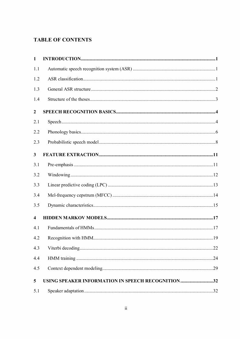
Consonants differ from vowels by a constriction or an obstruction that occurs in the pharyngeal or oral parts of the vocal tract. If vocal cords vibrate while producing consonant the sound is called voiced, otherwise unvoiced. Figure 2.5 illustrates a possible consonant classification if we consider the manner of articulation as a criterion.
8
Figure 2.5: English consonants classification based of the manner of articulation. [±V] denotes
voced/unvoised characteristics. Nasal consonants are caused by the airflow passing through the nasal cavity (opened by the velar). The oral cavity is closed at this time. The position of the oral cavity closure defines the sound being pronounced: lips (/m/), alveolar hump (/n/), close to the velum (/ng/). Semivowels are vowel-like sounds by their nature. They are highly influenced by the context they appear in. Fricatives are produced when almost complete blockage at some point in the oral cavity causes a turbulence of the airflow. A concrete fricative realization is conditioned to the position of the constriction. Stops are produced by rapid release of the airflow trapped by the complete closure in the oral cavity. This blockage occurs at the lips (/b/, /p/), back of teeth (/d/, /t/) or next to the velar (/g/, /k/). The class of complex consonants, which combine two manners of articulation, is called affricates, e.g. /ch/ in the word ‘church’ is a combination of /t/ and /sh/ sounds. Another way to classify consonants is “place of articulation” based. It can be found in [18] as well as manner-based classification described above. Information about phoneme classes becomes particularly important for building ASR system based on complex sub-word units (e.g. triphones).
2.3 Probabilistic speech model
A probabilistic model of a speech can be described as follows. A word sequence W produces observations X. The speech recognition system should decode this sequence of observations into words string. This decoded string will have a maximum a posteriori probability [34]:
)()|(maxarg)(
)()|(maxarg)|(maxargˆ WPWXPXP
WPWXPXWPWWWW
=== . (2.2)
P(X) was neglected because it does not depend on W. Term P(X|W) represents a probability of an observation sequence X subjected to the word sequence W. It is called an acoustic model. The second term is called a language model and evaluates a probability of a specified word sequence. It is especially useful for medium and large vocabulary systems and it brings a significant improvement in recognition rate. If we assume each word in the sequence independent from another we can write
Consonants
Nasals Semivowels
Fricatives Stops Affricates
Liquid Glide
[+V] v,z,dh,zh [-V] f,s,th,sh,hh
[+V] b,d,g [-V] p,t,k
[+V] jh [-V] ch
[+V] m,n,ng
[+V] l,r
[+V] w,y

9
∏=
=K
ii
i wXPWXP1
)|()|( , (2.3)
where wi is the i-th word in the sequence and X={X1, X2,…, XK}. Equation (2.3) is a whole-word modeling. Assuming further independence of phonemes, term P(X i|wi) can be written as
∏=
=M
jij
iji
i phXPwXP1
,)( )|()|( , (2.4)
where phj,i is a j-th phoneme in the i-th word and M is a number of phonemes in the i-th word. Equation (2.4) represents phoneme-based word models. Acoustic model P(X|W) estimates a sequence of observations conditioned to the word string [34]. It should take into account speaker and pronunciation variations, phonetic context-dependency, as well as to be able to be adapted to new environment or speaker. Hidden Markov Models discussed in the chapter 4 is a popular approach for acoustic modeling. Statistical Language Model (SLM) represents a probability of a word string W. In other words it shows how frequently W is met as a sentence. It is written in the form
∏=
−−=M
iiii wwwwpwpWP
21211 ),...,,|()()( , (2.5)
where sequence of the words wi-1, wi-2,… ,w1 is called the history and M is its length. Since it is impossible to estimate all word sequences given by equation (2.5), short histories are considered only. So the equation (2.5) can be approximated by N-grams language model:
∏=
+−−−≈M
iNiiii wwwwpwpWP
21211 ),...,,|()()( . (2.6)
History length defines the class of the SLM. Some examples are:
• Unigrams
∏=
≈M
iiwpwpWP
21 )()()( (2.7)
• Bigrams
∏=
−≈M
iii wwpwpWP
211 )|()()( (2.8)
• Trigrams
∏=
−−≈M
iiii wwwpwpWP
2211 ),|()()( (2.9)
The speech recognition scheme can be now summarized as illustrated in Figure 2.6.

10
Figure 2.6: Probabilistic speech recognition model.
The language P(W) and acoustic P(X|W) models are estimated from the training material. The former is out of the scope of this thesis while training techniques for the later will be considered further.
Acoustic model
Language model
FE Decoding Result
P(X|W)
P(W)
Training speech

11
3 FEATURE EXTRACTION The goal of feature extraction is to give a good representation of a speech signal capturing an important information about sounds pronounced. The modern feature extraction approaches are divided into production-based and perception-based methods. Linear predictive coding (LPC) belongs to the first group while Mel-frequency cepstral coefficients (MFCC) and Perceptual Linear Prediction (PLP) are the representatives of the perception-based approaches family. The LPC and MFCC techniques are considered in this section.
3.1 Pre-emphasis
Pre-emphasis is a process of passing the signal through a filter, which emphasizes higher frequencies. In speech signal, the most part of the energy is carried by the low frequencies. When the frequency increases pre-emphasis also increases the energy of the signal. It also serves to emphasis the formant peaks, to make them more “visible” in the spectrum. Figure 3.1 shows an example of pre-emphasis. On the left side of the figure, an unprocessed signal is plotted along with its short-time magnitude spectrum and spectrogram. The right side illustrates the same characteristics for the emphasized signal.
Figure 3.1: Unprocessed (left) and pre-emphasized (right) signals. As can be seen from the picture pre-emphasis makes the spectrum more flat by rising the energy in high frequency region. This effect is also well seen on the spectrogram where darker parts correspond to higher energy.

12
Pre-emphasis filter designed to compensate the effect of the glottal-source and energy radiation from the lips [21] when the spectrum of the recorded speech signal is 6 dB/octave lower than the original, i.e. vocal tract, spectrum. Such filter is implemented by the formula: ]1[][][ −−= naxnxny , (3.1) and its transfer function is given by: 11)( −−= azzH , (3.2) where a≈ 1.0 (e.g. 0,97).
3.2 Windowing
For extracting the spectral features of a speech signal a short-time analysis is applied [18]. The signal is assumed to be stationary within a short time interval, i.e. characteristics of the signal remain uniform and vocal tract parameters can be estimated. These regions are often referred to as frames and their length is around 20-25 ms. The frame length should be short enough to answer the assumption of the stationary signal and at the same time quite long to capture enough samples to calculate the parameters. The frames are also overlapped by approximately 10ms. To every frame a windowing function is applied to suppress the effect of discontinuities at frames edges. All the feature extraction techniques will analyze these windowed frames further. The most popular window is the Hamming window given by [18]:
≤≤−
=otherwise
NnN
nnw
,0
0,2cos46.054.0][
π. (3.3)
The process of framing and windowing is shown in Figure 3.2.
Figure 3.2: Short-time speech analysis.
Windowing
Feature vectors

13
3.3 Linear predictive coding (LPC)
LPC analysis is a popular technique in speech recognition. It provides a representation of a signal by a small number of parameters obtained by simple calculations [11]. The idea of LPC method is that a speech sample at time n can be represented as a linear combination of p previous samples weighted with some coefficients ak, where coefficients are constant over a single speech frame: ][...]2[]1[][ 21 pnxanxanxanx p −++−+−≈ . (3.4) A reasonable way to obtain ak is to minimize the squared error function
∑ ∑
−−=
=n
p
kkm jnxanxE
2
1
][][ . (3.5)
It can be done by taking the derivatives of Equation (3.5) with respect to ak and equating them to zero:
0=∂∂
k
maE
, pk ≤≤1 . (3.6)
The equation (3.6) becomes
]0,[],[1
iRkiRap
kk =∑
=
pi ≤≤1 , (3.7)
where ∑ −−=
nknxinxkiR ][][],[ . (3.8)
The equation (3.7) can be solved using autocorrelation method and Durbin’s recursion [18] obtaining the resulting algorithm for ak calculation:
1. Initialization E0=R[0]
2. Iteration For i=1,…,p do recursion:
11
1
1
][][ −−
−
−−= ∑
=
ii
k
iki EkiRaiRk (3.9)
iii ka = (3.10)
11 −−
− −= ikii
ik
ik akaa , pk ≤≤1 (3.11)
1)1( 2 −−= ii
i EkE (3.12)
3. Termination p
kk aa = , pk ≤≤1 (3.13)

14
LPC represents the spectral envelope by low-dimension feature vectors. For speech sampled by 8kHz the common choice is 10 LPC coefficients. A serious problem with the LPCs is that they are highly correlated. However, it is desirable to obtain less correlated features for acoustic modeling. In order to decorrelate LPC coefficients, LPC cepstral coefficients (LPCC) are used [2]: 1]1[ ac = , (3.14)
inin
in ca
nianc −
−
=∑ −+=
1
1)1(][ for 1<n<p, (3.15)
inin
ica
ninc −
−
=∑ −=
1
1)1(][ for n>p. (3.16)
Figure 3.3 summarizes the steps required for LPC and LPCC computations.
Figure 3.3: LPC and LPCC computation flowchart.
3.4 Mel-frequency cepstrum (MFCC)
There is an experimental evidence that the human perception of the frequency spectrum of sound does not have a linear characteristic. Taking auditory characteristics into account, the mel-scale frequency axis is often used. The relation between mel- and frequency in KHz is given by [11]: )1(log1000 2 fMel += . (3.17) Mel-frequency cepstral coefficients are defined as a discrete cosine transform of the log filterbank amplitudes. Each filter computes the average spectrum around each central frequency. An example of a filterbank used in MFCC calculations is shown in Figure 3.4.
Figure 3.4: Critical band filters used in MFCC computation and their outputs (s1 s2…sM).
Speech Preprocessing Autocorrelation Durbin’s
recursion LPC cepstrum computation
LPC coefficients
LPCC coefficients
1
Frequency
Magnitude
s1 s2 sM …

15
The MFCC computation involves the following steps:
1. Computing of the FFT-based spectrum
∑−
=
−
=1
0
2][][
NN
n
nkjenxkX
π, Nk <≤0 . (3.18)
2. Passing the magnitude spectrum X[k] through the mel filterbank. It is equal to multiply
each DFT magnitude coefficient by the corresponding filter value. The result of this step is the set of M values representing the energy in each band, where M is a number of filters in the filterbank.
3. Log-energy computation at the output of each filter
= ∑
−
=
1
0
2 ][]][[ln][N
km kHkXms , Mm <≤0 . (3.19)
4. Convert log-energies to the cepstral coefficients using discrete cosine transform (DCT)
∑−
=
−=
1
0))5.0(cos(][][
M
m Mmnmsnc π . (3.20)
It is seen from the formula (3.20) that c[0] can be considered as a total spectral energy. For speech recognition, the first 13 cepstrum coefficients are usually used. MFFC feature extraction approach gives a good discrimination and a small correlation between components. The basic idea of the cepstral analysis is to separate source and a filter in the signal and represent them as a linear combination [6]. It is important since the main interest of feature extraction in speech recognition is to estimate filter, i.e. vocal tract, parameters (see section 2.1.2). The cepstrum involves logarithm of the magnitude which results in summation of logarithms of source and filter magnitudes. After applying inverse discrete Fourier transform (or DCT in MFCC case) we get the characteristics of the slow-varying part (i.e. filter) concentrated in the low cepstral coefficients.
3.5 Dynamic characteristics
The vocal tract is characterized not by “static” parameters only (like LPCC or MFCC). During speech production, different articulators change their positions continuously. Measuring the character of these movements might be beneficial for speech recognition. The dynamic information of the speech spectrum is estimated by so-called delta-features. These characteristics can be computed as [18]: 22 +− −=∆ kkk ccc , (3.21) where ci is cepstral coefficient.

16
Replacing ck by Δck we get second-order derivatives which are called delta-delta or acceleration coefficients. Acceleration parameters are appended to each feature vector resulting in 3*N dimensional vector, where N is the number of LPCC or MFCC coefficients: FV=[ c1, c2,…, cK,, Δc1, Δc2… ΔcK, Δ2c1,, Δ2c2,…, Δ2cK]T.

17
4 HIDDEN MARKOV MODELS This chapter discusses the most popular approach in speech recognition - Hidden Markov Models (HMM). The following sections outline HMM basics and explain the main problems need to be solved in order to use HMMs for speech recognition tasks.
4.1 Fundamentals of HMMs
Hidden Markov Model is a stochastic state machine with a finite number of states [37]. It can be thought as a pair of stochastic processes: a hidden Markov chain and an observable process – a probabilistic function of the chain states [40]. At every time moment, HMM changes its state according to the state transition probabilities and omits an observation based on the probability density function (pdf) attached to the current state. The illustration of this process is given in Figure 4.1, where aij refers to the transition probability from state i to j, and oi is an output observation in the state i.
Figure 4.1: “HMM in action”.
HMM can be also thought as a “black box” generating some sequence of observations after some number of steps. The state sequence is “hidden” as we do not know which state has produced which observation. Applying HMMs for speech recognition causes an agreement with two main assumptions. First, it is assumed that the transition from one state to another depends on the current state and the state of destination only. This is known as a first-order Markov assumption. The second main assumption is an output-independent assumption: all observations are considered to be independent from each other and dependent on state they were generated by. Both of them are not valid for speech. However, in practice, involving second-order HMMs and taking into account correlations between speech frames did not show significant accuracy improvement. It also demands increase in computational complexity [18]. Formally, HMM is defined by the following parameters [33]: § The number of states in the model N § The set of all possible states in the model S = {s1, s2…sN} § The number of different observation objects M § Set of all possible objects observed V= {v1, v2… vM} § State transition probability distribution A= {aij}, where aij = P (qt+1 = sj | qt = si) (i,j ≤ N) § Observation probability distribution in state j, B= {bj(k)}, where
o1
4 3 2 a12 a23 a34 a45
a22 a33 a44
2 3 4
o2
a12 a23 a34 a45
a22 a33 a44
2 3 4
o3
a12 a23 a34 a45
a22 a33 a44
t=1 t=2 t=3

18
bj(k) = P(ot=vk |qt=sj) § The initial state distribution π = {πi}, where πi = P (q1=si).
In a compact form, HMM is defined as a triplet λ={A,B,π}. The parameter B will be also referred to as “state output function”, and it plays an important role in HMM theory as it defines the type of the HMM. Modeling of output spectral distributions is done using one of the following approaches:
• Discrete modeling • Continuous modeling • Semi-continuous modeling.
In the discrete case, the VQ approach (see Appendix A) is used for reducing the number of observations into a limited set of classes. In this case, every observation vector gets a label to show which class it belongs to. Therefore, a HMM state output function is just a histogram where each symbol has a probability emitted by a state. Applying VQ method, we always get a quantization error: some information in speech signal is lost. If we leave the data, i.e. feature vectors, as they are, without any changes, we can apply a continuous density HMMs. In this case, the output function is modeled using a pdf such as the Gaussian distribution [18]:
))()((
21
||)2(
1),;(μxUμx 1-
UUμx
−−−=
T
eNnπ
, (4.1)
where n is a dimensionality of vector x, µ is a mean vector and U is a covariance matrix. Since Gaussian is the unimodal distribution, i.e. it has only one “peak”, its modeling power is limited. The solution is to use mixture of Gaussians or Gaussian Mixture Model (GMM). Most of the modern continuous speech recognition systems are based on GMMs. The GMM output function for state j is given by:
∑=
=M
kjkjkjkj Ncb
1tt ),;()( Uoo µ , (4.2)
where cjk, μjk and Ujk are the weight, mean vector and covariance matrix of the k-th Gaussian component of the mixture in the j-th state and M is a number of Gaussians in the mixture. The coefficient cjk can be thought as a probability to choose k-th component in the mixture. Therefore, they have to satisfy the stochastic constraints:
11
=∑=
M
kjkc and 0≥jkc Nj ≤≤1 , Mk ≤≤1 . (4.3)
The semi-continuous (tied mixture) modeling case is a compromise between VQ and GMM. All output functions share the same set of mixture components, i.e. mean vectors and covariance matrixes stored in a codebook.

19
HMM in speech recognition is a template for recognition units. If, for example, the basic modeling unit for ASR is a word, then each HMM will be a template for single word, and recognition process converges to one illustrated in Figure 4.2, where an isolated word recognition case is assumed.
Figure 4.2: Isolated word recognition with HMMs λ2, λ2… λK.
Given a sequence of observations and set of HMMs, we can calculate which of the models has most likely produced this sequence. This is actually a speech recognition case: given models for units, we would like to know which HMM (or HMM string) matches the observation sequence better. Two main answers arise:
1. How to obtain a proper HMM for every modeling unit 2. Given HMM set, how to find the “best matcher” for a given observation sequence.
These questions actually correspond to the three basic problems of HMMs [34]:
1. Given a model λ and observation sequence O how to efficiently compute P(O|λ) (recognition problem)
2. Given a model λ and sequence of observations O, how to find a state sequence that has most likely produced O (decoding problem)
3. How to obtain HMM parameters λ= {A, B, π} to maximize P(O|λ) (training problem). The following sections discuss ways to answer these questions.
4.2 Recognition with HMM
The likelihood P(O|λ) can be calculated as follows. Let Q= {q1, q2…qT} be a fixed state sequence. Than the probability of the observations O and the state sequence Q given the model λ is [ ] [ ])()...()()...(),|()|()|,( 21 21132211 Tqqqqqqqqqq TTT
bbbaaaQPQPQP oooOO ⋅==−
πλλλ . (4.4) The probability of O given the λ is obtained by summation P(O,Q|λ) over all state sequences: ∑ ∑ −
==Q qqq
TqqqqqqqqqqT
TTTbaababQPP
...,21
2113222111
)(...)()()|,()|( oooOO πλλ . (4.5)
Using formula (4.5) we need to perform order of 2TNT calculations and therefore the equation (4.5) can hardly be used. There are more efficient algorithms for calculating the P(O|λ) value, namely forward and backward approaches [33]. Both of them are based on calculating auxiliary variables called forward and backward variables correspondingly.
Feature extraction
λ1 (word w1)
λ2 (word w2)
λK (word wK)
… Select
maximum
P(O| λ1) )
P(O| λ2) )
P(O| λK) )
w*=argmax(P(O| λK)) k
Speech

20
4.2.1 Forward algorithm
The forward approach iteratively computes the forward variable αt(i) which represents the probability of being in the state i at the time t and observe a partial sequence o1o2…ot given the model λ: )|,...()( 21 λα ittt sqPi == ooo . (4.6) The steps of the algorithm are summarized as follows:
1. Initialization )()( 11 oiibi πα = Ni ≤≤1 (4.7)
2. Iteration
)()()( 11
1 +=
+
= ∑ ti
N
jjitt baji oαα Ni ≤≤1 , 11 −≤≤ Tt (4.8)
3. Termination
∑=
=N
iT iP
1)()|( αλO (4.9)
The first step initializes forward variable α1(i) as a joint probability of two events: being in state si and observing the first element, o1, from the observation sequence. During the induction the variable αt(i) is calculated at each time moment t for every state i. The last step calculates the final result, P(O|λ), as a sum of αT(i) variables. Let us consider an example of 3-state HMM with continuous probability densities and one-dimensional feature vectors as illustrated in Figure 4.3. We will find the probability P(O|λ) using forward algorithm.
Figure 4.3: An example of 3-state HMM for modeling.
Let us assume that the observation sequence is O={o1, o2, o3}={‘y’ ‘eh’ ‘s’}. The Figure 4.4 shows the computation involved in the forward algorithm.
1 3
2
0.3 0.2 0.4
0.6 0.7
b1(‘s’)=0.2 b1(‘eh’)=0.3 b1(‘y’)=0.5
b2(‘s’)=0.2 b2(‘eh’)=0.7 b2(‘y’)=0.1
b3(‘s’)=0.8 b3(‘eh’)=0.1 b3(‘y’)=0.1
0.8

21
Figure 4.4: Forward algorithm proceeding.
So the total probability of the sequence O passed through the HMM given in the Figure 4.3 is P(O|λ)= 0.1422. In the next section, the same result will be obtained by another method called backward algorithm.
4.2.2 Backward algorithm
The idea of the backward algorithm is the same as that one of the forward algorithm. Instead of forward variable αt(i) it uses a backward one, βt(i). This variable is defined as the probability of the partial sequence started at (t+1), ot+1, ot+2…oT, given the state si at time t and model λ: ),|...()( 21 λβ itTttt sqPi == ++ ooo (4.10) This algorithm consists of three steps [33]:
1. Initialization
1)( =iTβ Ni ≤≤1 (4.11)
2. Iteration
)()()( 11
1 +=
+∑= t
N
jjijtt baji oββ Ni ≤≤1 , 11 ≥≥− tT (4.12)
3. Termination
∑=
=N
iii ibP
111 )()()|( βπλ oO Ni ≤≤1 (4.13)
Unlike in the forward algorithm the recursion works backward in time. We consider the result obtained for the moment of time (t+1) for all states, accounting for the transitions between them
0.5
0
0
0.06
0.21
0
Σ
Σ
0.0048
0.0198
0.1176
t=1 t=2
State 1
State 2
State 3
Σ
0.1422
P(O|λ)
α1(1)
α1(2)
α1(3)
α2(1)
α2(2)
α2(3)
α3(1)
α3(2)
α3(3)
*0.3 *0.4 Σ
*0.6
*0.3 *0.7
*0.7
*0.2 *0.1
*0.2 *0.4 Σ
*0.2
*0.6
*0.3 Σ
Σ *0.7
*0.2 *0.8
b1(‘eh’)
b2(‘eh’)
b3(‘eh’)
t=3
b1(‘s’)
b2(‘s’)
b3(‘s’)
Direction of computations

22
to the current state si (aij), observation ot+1 omitted in each of that state (bt+1(i)) and the remaining partial observation sequence ot+1, ot+2… oT from each state (βt+1(i)). The termination occurs when the recursion reaches the first state. As an example of this method we will consider the task presented in the previous section and illustrated in Figure 4.3. In the beginning the backward variable is initialized by the value of ‘1’: β3(2)=1, β3(3)=1 and β3(4)=1. Figure 4.5 illustrates the process of P(O|λ) calculating with backward algorithm.
Figure 4.5: Backward algorithm proceeding.
So, the result is the same as one obtained by the forward algorithm. The principal difference between these two approaches is that the backward case requires the information about the whole sequence of observations before starting its calculations For both forward and backward algorithms order of calculations is N2T. That is much better compare to “brute force” calculation given by equation (4.5). A forward variable, as well as a backward one, are involved in training Baum-Welch procedure. Since both algorithms obtain an exact value of P(O|λ) they can also be used for recognition.
4.3 Viterbi decoding
Since a set of states represents a hidden data in HMM, we can never know the exact sequence, which produced an observation sequence. However, the sequence, which has most likely produced the given observations, can be obtained via Viterbi algorithm. It goes like follows. First, we need to define the quantity [33]:
t=1 t=2
State 1
State 2
State 3
t=3
Direction of computations
1
1
1
β3(1)
β 3(2)
β 3(3)
0,2
*0.6
Σ *0.4 *0.2
*0.2
0,62 *0.3
*0.7 Σ *0.2
*0.8
0,16 *0.2 Σ *0.8
0,2844
*0.6
Σ *0.4 *0.3
*0.7
0,1414 *0.3
*0.7 Σ *0.7
*0.1
0,0032 *0.2 Σ *0.1
β2(1)
β 2(2)
β 2(3)
β 1(1)
β 1(2)
β 1(3)
*0.1
*0.1
*0.5 *1.0
*0
*0
Σ
0,1422
P(O|λ) bj(‘s’) bj(‘eh’)
bj(‘y’)

23
)|...,...(max)( 2121..., 121
λδ titqqq
t sqqqPit
ooo==−
. (4.14)
It is the highest probability along a single path, at time t, which accounts for the first t observations and ends in state si. In order to find the best state sequence we need to keep the argument which maximizes the δt(t). An array ψt(i) will be used for it. The steps of the Viterbi algorithm are given as follows:
1. Initialization )()( 11 oiibi πδ = , 0i =)(1ψ Ni ≤≤1 (4.15)
2. Iteration
)()(max)( 11
tijitNj
t baji o
= −
≤≤δδ , Ni ≤≤1 , Tt ≤≤2 (4.16)
])([maxarg)( 1
1jit
Njt aji −
≤≤= δψ , Ni ≤≤1 , Tt ≤≤2 (4.17)
3. Termination
)(max)|(
1* jP T
Njδλ
≤≤=O (4.18)
)(maxarg
1
* jq TNj
T δ≤≤
= (4.19)
4. Path backtracking
)( 1
*1
*++= ttt qq ψ , 11 ≥≥− tT (4.20)
The Viterbi procedure is similar to the forward algorithm. The only difference is the substitution of the summation with maximization operation over previous states. The Viterbi algorithm is a form of the dynamic programming method [11]. An example of Viterbi best state sequence searching for the example given above is shown in Figure 4.6.

24
Figure 4.6: Viterbi algorithm proceeding. The resulting state sequence is 1-2-3.
Using the formulas given above leads to extremely small probability values during calculations and therefore underflow problem occurs. In order to avoid it the observation probability at each step is usually represented in a logarithmic form [43]: [ ] ( ))(log)log()(max)( 1
1tijit
Njt baji o++= −
≤≤δδ . (4.21)
Although the value of P*(O|λ) is a likelihood of O through one path only, it can be also used for recognition purposes as it can be considered instead of the total likelihood obtained by forward or backward methods for recognition purposes.
4.4 HMM training
The goal of the training step is to find the parameters of the model λ={π, A, B} such that the likelihood of training data P(O|λ) is maximized. Before starting the training process we need to define the following:
• HMM’s topology (type) • Method for observation modeling, i.e. the type of output function • Initialization.
The choice of the topology is rather straightforward: left-to-right model with self-loops is commonly used [18]. Such structure reflects the speech as a continuous process in time and self-loops model quasi-stationary segments is speech when parameters do not vary much. The number of states in the model is chosen taking into account the modeling unit. For instance, if the goal is to model full words, the number of states can be chosen depending on the word length, while for phoneme modeling three state models is commonly a good choice [43].
0.5
0
0
0.06
0.21
0
max
max
0.0048
0.0126
0.1176
t=1 t=2
State 1
State 2
State 3
max
0.1176
P*(O|λ) q3
*=3
δ1(1) ψ1(1)=0
δ 1(2) ψ1(2)=0
δ 1(3) ψ1(3)=0
δ2(1) ψ2(1)=1
δ 2(2) ψ2(2)=1
δ 2(3) ψ2(3)=2
δ 3(1) ψ3(1)=1
δ 3(2) ψ3(2)=2
δ 3(3) ψ3(3)=2
*0.3 *0.4 max
*0.6
*0.3 *0.7
*0.7
*0.2 *0.1
*0.2 *0.4 max
*0.2
*0.6
*0.3 max
max *0.7
*0.2 *0.8
bj(o2)
t=3
bj(o3) aij aij

25
The choice of the type of output pdf is less obvious. Discrete HMM quantizes observations that can lead to degradation in recognition. On the other hand, discrete HMMs can outperform continuous HMMs in decoding speed as demonstrated in [7]1. Therefore, there is probably no clear answer, which HMM type should be preferred, and this choice depends on the actual requirements for ASR system. The HMM parameters are initialized before the actual training procedure started. In general, the initialization can go by one of the following ways:
• So called “flat start”, i.e. all models are identical. For example, the global mean and variance can be computed and assigned as initial estimates for each model [43]. Initial values for state transitions are assigned by hand, randomly or uniformly subjecting to certain constraints.
• Segmental k-means algorithm. It uses Viterbi algorithm to strictly assign each feature vector to some state, i.e. it creates a state-frame alignment. Having such alignment we can calculate initial values for transitions and Gaussian parameters.
• Another way is to use an existing HMM set, which is already trained for some task.
When the issues mentioned above are decided and feature vectors obtained we can start training acoustic models. There are at least two methods available for HMM training [33]:
1. Segmental k-means algorithm 2. Baum-Welch algorithm
Both the Baum-Welch and the segmental k-means approaches are examples of the maximum likelihood estimation (MLE) [18]. MLE assumes that the training data is large enough and can be used to find robust estimates of the model parameters.
4.4.1 Segmental k-means algorithm
This algorithm is often used for initializing the parameters of HMM. At the same time, it can be used as a training method itself. The steps of algorithm are summarized as follows:
1. Divide each of the training utterances arbitrarily into N segments, where N is the number of states in the HMM. Flat start, manual alignment or force alignment approaches are available.
2. Given vectors corresponding to one segment split this state into M regions Vjk (j=1…N, k=1…M) using VQ, where M is a number of mixtures being used for modeling the states output functions.
3. For each mixture component in each segment (Vjk) compute new values for means and covariance matrices:
j
jkjk N
Nc = , (4.22)
jkjk xμ = , (4.23)
1 Actually, in [7] authors invented a discrete-mixture HMM which can be thought as an extension of conventional discrete HMM.

26
∑∈
−−=jkt V
jktT
jktjk
jk NU
ooo )()(1 xx , (4.24)
where Njk is the number of vectors in Vjk segment, Nj is the number of vectors in the whole segment j and xjk is a centroid of Vjk.
4. Given the new parameter estimates, re-segment each training utterance into states using Viterbi algorithm. If the distance, which represents the statistical similarity between new and old models, exceeds some threshold the algorithm is repeated from the 2nd step.
Updated values for aij are obtained by dividing the number of transitions from state i to j by the number of transitions from state i to any state (including itself). Let us consider an example of k-means segmentation shown in Figure 4.7. We will construct 3-state HMM, in which the output density function is represented as a mixture of 2 Gaussians. In the first step, we divide the training utterance into N=3 equal parts. This is an example of the “flat start” approach. The second step performs splitting of every state into M=2 regions using VQ. Our next goal is to calculate new values for mixture coefficients cjk, mean vectors μjk and covariance matrices Ujk for every state. This is done on the third step. After that, the Viterbi algorithm is applied. It re-segments the data and if the new model differs from the previous one, i.e. if a distance score that reflects the statistical similarity of the HMMs is larger than the threshold, the algorithm proceeds from the second step.
Figure 4.7: Segmental k-means algorithm example.
1st step. Select initial states 2nd step. Each state is clustered into 2 regions using VQ
3rd step. New values for cjk, μjk and Ujk are calculated.
4th step. An example of a probable data re-segmentation with VQ and the parameter recalculations applied. Some of the feature
vectors have changed the states they belonged to.

27
4.4.2 Baum-Welch algorithm
The task of maximizing P(O|λ) does not have a closed-form analytical solution. An iterative Baum-Welch algorithm is used instead. It locally maximizes P(O|λ) applying ideas of the expectation maximization (EM) algorithm [3] to HMMs parameter estimation. To describe the re-estimation process, we need to define two auxiliary variables [34]. The first one represents the probability of being in i-th state at time t and in j-th state at time (t+1), given the model and the observation sequence: ),|,(),( 1t λξ OjsisPji tt === + . (4.25) The second variable, often referred to as a state occupation, defines the probability of being in state i at time t given the model and the observation sequence: ),|()( λγ OisPi tt == . (4.26) In terms of forward and the backward variables, ξt(i,j) and γt(i) can be expressed as:
∑∑= =
++
++++ ==N
i
N
jttjijt
ttjijtttjijtt
jbai
jbaiP
jbaiji
1 111
1111
)()()(
)()()()|(
)()()(),(
βα
βα
λ
βαξ
o
oOo
, (4.27)
∑=
==N
itt
ttttt
ii
iiP
iii
1)()(
)()()|()()(
)(βα
βαλ
βαγ
O, (4.28)
where P(O|λ) is a normalization factor. There is a relation between these two variables:
∑=
=N
jtt jii
1),()( ξγ . (4.29)
Now, if we sum up γt(i) over T, the quantity we will get is an expected number of times the state si was visited. Similarly, sum of ξt(i,j) represents an expected number of transitions from state si to sj. In a case of GMM, the quantity
=
∑∑==
M
mjmjmtjm
jkjktjkN
ntt
ttt
Nc
Nc
nn
jjkj
11),,(
),,(
)()(
)()(),(
Uμo
Uμo
βα
βαγ (4.30)
is an estimated number of times the k-th mixture of the j-th state was occupied at time t.

28
Using the expressions (4.25) and (4.26), the following formulas for the HMM parameters can be obtained. Transition probabilities
∑
∑
∑
∑−
=
−
=−
=
−
−
=
−+
=
=
==
= 1
1
1
11
1
)1(
1
1
)1(1
)(
),(
)|,(
)|,,(
T
tt
T
tt
T
t
it
T
t
itt
ij
i
ji
iqp
jqiqpa
γ
ξ
λ
λ
O
O. (4.31)
For continuous HMMs the formula for aij is identical to those in a discrete case. State output function
• Discrete case
∑
∑
∑
∑
=
==
=
−
==
−
=
=
=
=T
tt
T
vtst
t
T
t
it
T
vtst
it
j
j
j
jqp
jqp
kb ktkt
1
..1
1
)1(
..1
)1(
)(
)(
)|,(
)|,(
)(γ
γ
λ
λ
oo
O
O
. (4.32)
• Continuous case
∑∑
∑
= =
== T
t
M
kt
T
tt
jk
kj
kjc
1 1
1
),(
),(
γ
γ, (4.33)
∑
∑
=
=⋅
= T
tt
T
kttt
jk
kj
kj
1),(
),(
γ
γ oμ , (4.34)
∑
∑
=
=−−⋅
= T
tt
T
t
Tjktjktt
jk
kj
kj
1
1
),(
))((),(
γ
µµγ ooU , (4.35)
where state is denoted by j and k refers to the mixture component.

29
Every step of re-estimation of the model λ using formulas (4.31)-(4.35) results in a new model λ’ such that P(O|λ’)≥ P(O| λ). It means that the new model is guaranteed to represents the same or a better fit to training data. Comparing two training strategies, we can notice that k-means segmental algorithm makes hard decision about observations and state alignment, while Baum-Welch involves states occupations taking thus soft decision. The observations in the last case are assigned to the state proportionally to the probability the HMM was in that state when this observation occurred.
4.5 Context dependent modeling
Before training HMMs we need to decide what kind of acoustic units they represent. One possible choice is whole word modeling. In this case each HMM corresponds to one word and hence the number of models increases with the vocabulary size. For small vocabulary tasks like digit recognition whole-word modeling can be used, but for large vocabularies such models are not convenient anymore and sub-word units are used instead. Phone is a common choice. Using phones also reduces the size of ASR and allows recognizing the words, which do not appear in the training data. The amount of phonemes is limited but the number of their variations is huge because of different surrounding phones. So called context-dependent modeling tries to catch a context the phone occurs in. Taking into account left and right phones, we get a triphone system. The phone will be also referred to as monophone denoting context independent unit. There are two strategies of expanding phones to triphones: within-word and cross-word (see Table 4.1). In the former case, monophones are not expanded through words boundaries, while in the latter case word boundaries are ignored.
Table 4.1: Within- and cross-word expansion example for the first two words in the sentence “The emperor had a mean temper”.
Word Phoneme transcription
Within-word expansion
Cross-word expansion
dh dh+ah dh+ah The ah dh-ah dh-ah+eh pause sp sp sp
eh eh+m ah-eh+m m eh-m+p eh-m+p p m-p+er m-p+er er p-er+er p-er+er
Emperor
er er-er er-er+hh pause sp sp sp
… Simple calculations show that for a 39 phone set, the theoretical number of possible triphones is 59319. Getting a sufficient training data for all contexts is not possible in practice. To solve this problem one can use tree-based clustering. Its idea is to pool similar states into one cluster and consider it as one state. The algorithm block scheme is shown in Figure 4.8 [32].

30
Figure 4.8: The tree-based state clustering algorithm flowchart.
The phonetic decision tree is a binary tree with questions attached to each node [43]. These questions have two answers only: yes and no. The goal is to find a question that maximizes an increase in data likelihood. An example set of questions is: Q1: Is the left context stop consonant? Q2: Is the left context central consonant? Q3: Is the right context fricative? Q4: Is the left context vowel? etc. After every splitting step, the data likelihood in the two created children nodes will be larger than in the parent node since the same data is modeled by twice larger number of parameters. The question should maximize this difference. It should be mentioned here that in order to calculate an increase in the log likelihood we do not need actual observations. Means, covariance matrices and occupancies of states in a cluster can be used instead. A minimal occupancy threshold ensures that no outlier cluster is created and all clusters with occupancy below this threshold are merged with their nearest neighbors. In summary, for the tree-based clustering one needs to specify the following:
Pool all states in the root node
Re-estimate HMMsparameters
N
N
Y
Y
Find a node and a question, which maximizes the increase of log likelihood after splitting
Increase exceeds
threshold?
Split the node found
Choose two leafs, which give minimum decrease in likelihood if merged
Decrease is less than
threshold?
Merge nodes found

31
• Set of phonetic-based questions for splitting • Threshold for log likelihood increase • Threshold for minimum state occupancy • The likelihood of the data given pooled set of tied states.
Figure 4.9 illustrates tree-based state clustering example for the central state of all triphones of the ‘ao’ phone. Questions Q1, Q2 … are assumed to be the “best” ones within corresponding node. The set of questions applied was given above.
Figure 4.9: Tree-based state clustering example for the central state of ‘ao’ triphones.
Q1: L=stop consonant?
Q3: R=fricative?
Q4: L=vowel?
t-ao+s f-ao+l n-ao+z
f-ao+l n-ao+z t-ao+s
Y N
t-ao+s
Y N Y N
f-ao+l n-ao+z
t-ao+s
f-ao+l
n-ao+z ...
…
… …
…

32
5 USING SPEAKER INFORMATION IN SPEECH RECOGNITION All speech recognition systems can be divided into three classes based on speaker constraint introduced to them. These classes are speaker independent (SI), speaker adaptive (SA) and speaker dependent (SD) systems. If the training material relates to one speaker only, the models built are considered speaker dependent. Usually thousands of training utterances are needed to build well trained acoustic models, and they hardly can be taken from a single person. So training data from many different speakers is used to obtain speaker independent HMMs. These HMMs have larger variances than speaker dependent ones, and hence, we can say they are “averaged” among all speakers. Since an error rate for such systems is significantly higher than for ones trained to one speaker (a WER reduction can reach 50% [16]), adaptation techniques were developed to fill this gap. Adaptation methods are aimed to adjust the parameters of “averaged” models to better fit a current testing speaker based on small speech material from him only. In other words, speaker adaptive systems are obtained by “moving” speaker independent models towards dependent ones. Another way to involve speaker constraints in speech recognition is clustering [24], [36], [31]. The main idea is to create clusters of similar speakers, and train separate HMMs for every cluster or use data from the cluster as an adaptation material. In both cases, speaker clustering and matching are needed. In the case of clustering, an adaptation for a speaker is done by selecting the most “close” cluster or a group of clusters.
5.1 Speaker adaptation
Depending on the conditions an adaptation can be: • Supervised or unsupervised. If we are given an exact transcription of the adaptation data,
adaptation is done in a supervised mode, otherwise in an unsupervised one. • Static or dynamic. If the adaptation data is available as one block, adaptation is said to be
static. Otherwise, it can be done incrementally. According to [19] there are three groups of adaptation techniques in state-of-the-art speaker adaptation:
• Linear transformation family • Bayesian learning family • Speaker space family.
The first group is represented by the maximum likelihood linear regression (MLLR) method [27] and its extensions. MLLR aims to find the “best” transformation of parameters which brings speaker independent model closer to speaker dependent one. The main representative of the Bayesian learning family is maximum a posteriori estimation (MAP) technique [13]. An adaptation process here is driven by prior information about existing models. Speaker space family is represented by eigenvoices approach [25]. The idea behind this method is to use a “speaker basis” (eigenvoices), derived from the training data, and to represent any test speaker as a weighted combination of them.

33
5.1.1 Maximum a posteriori estimation (MAP)
The MAP approach incorporates an idea of combining prior knowledge of model parameters and some limited adaptation data. Suppose that we have observed a sequence of random samples {x1, x2… xN} which are distributed with a pdf p(x|λ), where λ is a parameter vector. The posterior distribution for λ is defined as [18]:
)(
)|()()|(xpxppxp λλ
λ = . (5.1)
For maximization of (5.1) we can drop the denominator because it does not depend on parameters λ. While the maximum likelihood estimation deals with the likelihood of training data p(x|λ), the MAP approach considers a posterior distribution p(λ)p(x|λ). The prior distribution p(λ) is considered as a knowledge of λ before the observations are available. The MAP estimation incorporates prior information in the learning process. The presence of prior distribution p(λ) means that less data is needed for robust parameter estimation and therefore MAP is useful for speaker adaptation. The mathematical derivation of MAP formulas can be found in [13]. For instance, the result for mean value of one Gaussian is:
∑
∑
=
=
+
+= T
t
T
t
t
t
1
1t0
)(
)(ˆ
γτ
γτ oμμ , (5.2)
where μ0 is a mean of the prior Gaussian, γ(t) is an occupation count of this Gaussian at time t, ot is observation vector and τ is a parameter measuring the “faith” in prior model. Equation (5.2) represents a weighted sum of the prior mean μ0 and ML mean estimate and can be interpreted as a balance between prior and new data. Parameter τ is a balancing factor between the prior mean and ML estimate [18], and if it is set to zero we get the pure ML estimation as a special case. When the amount of training data approaches to infinity, the MAP converges to ML estimation and the estimated model converges to the speaker dependent one. The main disadvantage of this method is that it is a local approach, i.e. it modifies those parameters only, which are observed in the adaptation data. In order to overcome this problem some extensions of MAP are proposed. For example, the regression-based model prediction (RMP) approach [1] calculates intra-Gaussian correlations on the training stage. During adaptation, it updates observed Gaussians with MAP and the rest using estimated correlations.
5.1.2 Maximum likelihood linear regression (MLLR)
In the MLLR approach, the idea is to transform linearly the model parameters to obtain an adapted model. The adaptation of mean vector of each Gaussian component is performed via linear regression-based transform [42]: WξbAμμ =+=ˆ , (5.3)

34
where W is a transformation matrix dimension n × (n+1) and ξ is an extended mean vector ξT=[1,μ1… μn], where μi is the i-th component of the mean vector μ. The matrix W is estimated to maximize the likelihood of the adaptation data. The mathematical derivations and the resulting formulas can be found e.g. in [27]. The computation of the matrix W is expensive. In order to make it more efficient, we can use a diagonal transformation matrix. However, as mentioned in [28] the full matrix gives better results. Applying MLLR to means results in changing the location of mixture components in the acoustic space preserving their shapes as it is depicted in Figure 5.1.
Figure 5.1: MLLR adaptation for means.
The main advantage of MLLR compared to MAP is its ability adapt to “unseen” Gaussians. This is done by tying mixture components to regression classes based on their acoustic similarity. The idea behind this is that acoustically similar components are supposed to share the same transformation so that they move in the same direction. In Figure 5.1 there are two regression classes and mixtures belonging to each of them transformed similarly. This allows using a small amount of adaptation data effectively. Gaussians can be grouped e.g. at the phone level and arranged in hierarchical structure. Example of such a regression class tree is shown in Figure 5.2.
Figure 5.2: Regression class tree for MLLR. Wi denotes the transformation matrix shared by the
specific class. The special case is a global MLLR adaptation when one transformation is applied to all Gaussians. Another way to construct the tree is a centroid splitting algorithm [43]. According to the MAP and MLLR comparison given in [18], the transformation-based approach outperforms MAP for smaller number of adaptation utterances (<400). However, when the amount of the adaptation data increases, MAP gives better results, since it converges to ML
Regression class 1
Regression class 2
New locations of mixtures after linear
transformations
All speech
Consonants Vowels
Voiced Unvoiced Front Back
W
Wc Wv
Wcv Wcu Wvf Wvb

35
estimates. These two methods can be combined by using first a global MLLR estimation, followed by MAP [43].
5.2 Speaker clustering
Different factors influence speaker’s acoustic characteristics. It includes gender, speaking rate and dialect differences. Speaker clustering aims to group similar speakers together in order to reduce speaker variability within each cluster. In the recognition phase, the cluster, which is the closest one to the target speaker is selected and utilized in recognition. The general schema of using speaker clustering in speech recognition is shown in Figure 5.3.
Figure 5.3: Speaker clustering utilized in speech recognition.
The steps of developing system outlined in Figure 5.3 can be summarized as follows:
1. Using training material from a large number of speakers, create speaker clusters. 2. Estimate acoustic models for each cluster. There are two commonly used approaches:
a) Training HMMs for every cluster to get “cluster-dependent” set of models b) Using cluster’s data, perform adaptation (MLLR, MAP) of the speaker
independent HMMs. 3. During recognition, the cluster that matches the current speaker better is determined, and
its HMMs are used for actual recognition. The first and second are done during development phase and the last one is a recognition itself. A fundamental issue is the selection of clustering approach to be used. Dividing the speakers into groups can be done either manually or by automatic clustering algorithms. The most straightforward, and an efficient clustering is a gender-based one. The fundamental frequency as well as formant frequencies varies a lot among genders and numerous algorithms for gender identification utilize this fact [41]. Gender-based clustering approaches give an improvement to the performance, but the number of clusters is restricted to two. In order to create an arbitrary number of groups, automatic clustering methods are used.
Cluster N representative
Cluster 1 representative
…
Cluster dependent
HMMs …
Cluster dependent
HMMs
FE Cluster identification
Speech recognizer
…
Cluster 1 Cluster N
Transcription
Cluster index
Speech

36
For speaker clustering we need to fix the following: • Cluster representative • Distance measure, i.e. how to measure the closeness between speakers and clustering
units representatives In our case, the cluster representative should be a characteristic of a speaker that represents the cluster. Speaker representations can be divided into two groups: model-based representations via GMMs, HMMs or Hidden Markov Nets (HMNets) [36], [24], and non-parametric ones, such as estimated vocal tract (VT) parameters [31]. Choice of the distance or similarity measure depends on the chosen speaker representation. For the model-based representation, this is usually likelihood measure. For the non parametric case, the Euclidean distance is popular. Training cluster-dependent HMMs requires a large amount of data for each cluster. It is not always possible to get enough data for training. One of the ways to overcome this problem is clustering in combination with adaptation techniques, e.g. instead of training cluster-dependent acoustic models they can be obtained by adapting speaker independent ones.
5.2.1 Related work
Both [24] and [36] represent tree-based speaker clustering. In [24], speaker-dependent HMNets and Bhattacharyya distance measure between them are involved in building a top-down tree. The clustering procedure divides nodes with the maximum sum of distances at each step until the average distance between centroid and each HMNet in the cluster is less than predefined threshold. A centroid HMNet is chosen as one with the minimum sum of distances. Adaptation proceeds as follows: at every depth (tree level), the best HMNet is found using an adaptation utterance and used for recognition. This can be considered as an adaptation method in which no parameter transformation is done. The authors reported that this method reduces the error rate by 8.5%. In the method proposed in [36], a speaker tree is created based on GMMs trained for each speaker. Relative entropy is used as a distance measure. The building process starts from the leaves and the two closest nodes are merged at each step (i.e. bottom-up approach). Thus, each node represents a speaker cluster. Cluster-based HMMs are either trained, or obtained via adaptation of a SI system based on the data assigned to the cluster. During evaluation, the closest cluster (i.e. tree node) is determined, and the corresponding HMMs are used in recognition. As an alternative approach the authors considered “leave” clusters only, i.e. ones representing individual speakers from the training set. A predefined number of these clusters which are the closest ones for target speaker are picked up and models for recognition are built by averaging means and variances of ones corresponding to chosen clusters. 5% improvement over speaker independent baseline system was achieved in this case. A nonparametric approach was proposed in [31]. This method uses 2-dimensional vocal tract (VT) parameters: lengths of the oral and pharyngeal sections. First, these parameters are estimated for every training speaker using a mapping procedure. The next step is to create clusters based on estimated VT parameters by the LBG algorithm. Adaptation process is performed by selecting the best cluster and using its acoustic models for testing. Authors

37
suggested two ways of making a decision about what cluster the target speaker belongs to. First one is based on the Euclidean distance between speaker’s VT parameters and ones averaged among all speakers belonging to the cluster. The second one is the maximum likelihood criterion based approach when the recognition starts with not one but several cluster dependent HMMs and during testing models with the highest likelihood are chosen. The method was tested for phoneme recognition task and 11% of error reduction compared to baseline was obtained for the first recognition approach. At the same time, the likelihood-based cluster selection method was shown to provide no sufficient improvement. Clustering approaches mentioned above use hard clustering when new speaker is assigned to one cluster. As an extension of this approach soft clustering techniques were proposed. Examples of soft clustering techniques are cluster adaptive training (CAT) [12] and eigenvoices mentioned above. Eigenvoices have got an intensive interest recently due to their particular effectiveness for rapid speaker adaptation [26]. The steps involved in finding eigenvoices are (training set consists of N speakers) [25]:
• For N speakers in the training set obtain N speaker dependent HMM sets • For each speaker a supervector is composed. Each HMM contributes in this vector by
mean vector from every mixture component of every HMM state • For all N supervectors mean and covariance matrix are computed • Apply the principle component analysis (PCA) to get N eigenvoices • Select first K eigenvoices.
Now a new speaker is represented as a weighted sum of K eigenvoices. The weights are obtained via maximum likelihood eigen-decomposition (MLED) [25]. Another way to exploit the eigenvoice ideas is presented in [8]. The speaker clustering based on speaker specific weight vectors, estimated by MLED, is done using bottom-up approach and simple distance measure: dij=|wi - wj|, (5.4) where wj and wi are the weights obtained for i-th and j-th speakers. The distance between two clusters is defined as a maximum dij between all speakers from these clusters. Bottom-up clustering approach assumes merging two clusters with the minimal distances. It stops when the desired number of clusters achieved. As reported in [8], for K=2 eigenvoice case this method leads to clear male/female separation. The best result was obtained for 8 clusters and showed 29.1% WER compare to 31.2% baseline result (i.e. 6.7% relative error reduction). An interesting way of incorporating speaker information into speech recognition is a combination of speaker and speech recognition [17], [9]. In [17], this combination is considered as a joint maximization of a posteriori probability of a speaker and word sequence, given the observed speech. A possible application for this framework is spoken identity claims. In [9], a framework for adaptive speech recognition integrated with speaker identification is presented. Authors propose to use GMMs for speaker recognition. If it is known a priori which speakers can appear during testing, then GMM and adapted acoustic models are created for them. On the recognition phase the system checks if the target speaker’s GMM is already created. If it

38
is, the system performs decoding on “speaker-adapted” acoustic models. Otherwise, (an unknown speaker) the system creates a new GMM for him/her and adapts speaker independent models using a short part of the utterance. The main advantage of speaker recognition involvement into speech recognition task is the fact that short utterance, e.g. 3 seconds, is still too short for good speaker adaptation while speaker recognition has achieved reliable results even for such limited test material [23]. In combination with speaker clustering it can lead to fast speaker cluster detection and thus fast speaker adaptation.
5.2.2 Proposed codebooks clustering
Model-based speaker clustering approaches proposed in [36], [24] and outlined above, describe speakers models by HMMs or GMMs. We propose to use a simple approach based on speaker models generated using VQ (see Appendix C). The advantages of much simpler distance measures and computation effectiveness of VQ approach for real-time speaker identification can be exploited. The method proposed here is a combination of VQ-based speaker recognition and clustering techniques. The method of VQ model grouping will be referred to as metaclustering. The choice of this name follows from the fact that the objects for clustering, i.e. speakers codebooks, are results of clustering by themselves. Metaclustering exploits ideas from the k-means clustering algorithm (see Appendix A) extended to codebooks. Input parameters for this method are:
• X[N] is an array of N codebooks. Each codebook contains K vectors of the same dimension
• M is a number of clusters required • T is a number of k-means iterations
A block scheme for this method is shown in Figure 5.4. Initial steps and one iteration are illustrated in Figure 5.5 for the case of N=5 and M=2. Theoretically, metaclustering can perform on full feature vector set but it would strongly slow down the clustering procedure.

39
Figure 5.4: Flowchart of the proposed metaclustering algorithm.
The metaclustering algorithm utilizes all steps from the conventional k-means. The key differences are the procedures of finding cluster representatives and partitions. The idea in the former one is to find a “centroid codebook” and treat it as a representative of the cluster. This is done by pooling all codebook vectors from one cluster together and performing any clustering procedure on this merged vector set. We use the Randomized local search algorithm [10] for obtaining the centroid codebook from the pool of vectors.
Figure 5.5: Steps involved in metaclustering. Step 3 and 4 represent one iteration of the
algorithm while the first two steps are initialization.
Begin
Select randomly M representative codebooks into meta-codebook C
Generate partition P for C
i=0
i<T
Find representatives C’ for the current partition P
Generate partition P’ for the new representatives C’
P=P’
End
yes
no
i=i+1
Step 1. Select randomly N codebooks
Step 2. Generate partition P
Step 3. Find representatives C’ for
every cluster
Step 4. Generate new partition P’ for C’
* ** **
* ** **
*** ** *** **

40
The procedure of finding the optimal partition assigns every data codebook to the closest centroid codebook. The “closeness” of two codebooks X and Y is measured using the following symmetric distance measure: ),(),(),( XYYXYX distdistD += , (5.5) where dist(X,Y) is calculated as a sum of minimum distances between every vector in X and every vector in Y. The measure (5.5) is shown to be a distance function since it is nonnegative, symmetric and zero if and only if X=Y [20]. A pseudocode for computing the sum of minimum distances dist(X,Y) is given below.
Figure 5.6: Calculation of the distance between two codebooks.
The whole scheme of the training/recognition process with VQ codebooks clustering is shown in Figure 5.7.
Figure 5.7: Involving metaclustering in training process.
Training material
(N speakers)
Feature extraction
FV set 1
FV set 2
FV set 3
FV set N
Create codebook for every FV set
CB 1
CB 2
CB 3
CB N
Meta-clustering
Number of clusters (M) Centroid
CB 1
M centroid codebooks
Centroid CB 2
Centroid CB M
function dist(X,Y) {
sum := 0; FOR every vector xi in X DO {
d := EuclideanDist(xi, y1);
FOR every vector yj in Y DO {
IF (d > EuclideanDist(xi, yj)) {
d := EuclideanDist(xi, yj); }
}
sum := sum + d; }
return sum; }

41
First, feature vector sets (FV sets) are extracted from the speech material of every speaker. Based on these feature vectors, VQ-based speaker modeling is used for producing the speaker codebooks (see Appendix C). After that, metaclustering is performed on these codebooks as it was described above. The results of the metaclustering are the M cluster-dependent centroid codebooks and the partitioning, i.e. information about which clusters each speaker belongs to. After this, HMM training/adaptation is performed for every cluster based of the data assigned to it. The recognition process is going as it was illustrated in the Figure 5.3. Cluster identification is simply a speaker identification procedure as explained in Appendix C, which treats the centroid codebooks as cluster representatives. It should be noted here, that for recognition purposes we do not need to create test speaker model, just feature vectors are in use.

42
6 SPEECH RECOGNITION SYSTEM BUILDING
6.1 HTK description
Hidden Markov Toolkit (HTK) [43] is a software toolkit developed at Cambridge University. It provides a wide set of functions and programs for working with both continuous and discrete HMMs. This toolkit is meant for speech recognition tasks mostly. Hand-written text and speaker recognition systems can be implemented using HTK as well. The toolkit consists of four major groups of tools: data preparation, training, testing and analyzing tools. Figure 6.1 gives and overview of the HTK structure.
Figure 6.1: The main parts of HTK: training and recognition tools.
6.2 Training
The philosophy of the HTK is to build a recognition system incrementally, step by step. Sound files and their transcriptions are necessary for the training phase. If phone level transcriptions are not available, they can be obtained from the word level transcriptions and a lexicon using HTK tool HDMan. The sequence of steps used for ASR building is illustrated in Figure 6.2.
Transcriptions test1.wav bye test2.wav hello …
Training tools (HErest, HCompv etc.)
Training speech hello.wav bye.wav …
Transcriptions hello.wav hh ah l ow bye.wav b ay …
Recognition tools (HVite) Unknown speech test1.wav test2.wav …

43
Figure 6.2: Steps of ASR building using HTK.
Feature extraction HCopy
Training speech
Transcriptions
Flat start HCompv
HMM reestimation 3xHErest
Fixing silence model
HVite
HMM reestimation 2xHErest
Data realignment HVite
HMM reestimation 2xHErest
Triphone set generation HLEd, HHEd HMM reestimation 2xHErest
Tree-based clustering HHEd HMM reestimation 2xHErest
Triphone-based models, one mixture per state
Monophone-based models, one mixture per state
Mixture incrementing HHEd HMM reestimation 2xHErest Triphone-based models,
N mixtures per state

44
Feature extraction (HCopy) The first step for any ASR building is a feature extraction from the training speech. This is accomplished by HTK tool HCopy. We need to specify parameters for speech processing (like what kind of features we would like to obtain, window size, window shift, number of mel filters etc.) and list of sound files the features will be extracted from. Flat start (HCompV) First, a monophone-based system was built using 5-state left-to-right HMMs with three emitting states and one mixture per state (see Figure 6.3).
Figure 6.3: HMM with three emitting states used for monophones. Feature extraction and determination of HMM structure are followed by the training phase. First, we need to obtain initial parameter values. This can be done by HTK tool HCompV. It calculates a global covariance and mean, and assigns these values to all states in the model. When such “prototype” model has been initialized, it is duplicated for every monophone used in the system. Parameter estimation (HErest) HMM training in HTK is carried out by the HErest tool. It does not require any information about phone boundaries in the word and performs so called embedded training, which means that all models are updated simultaneously. First, every sentence is represented as a word string. Then each word is composed of the corresponding phonemes according to its pronunciation. Next, this phoneme-level chain is transformed into model-level chain. It is done by substituting every phoneme by corresponding HMM. Figure 6.4 illustrates this process. A forward-backward training is then applied to this composite HMM.
Figure 6.4: Creating a composite HMM for embedded training.
2 3 4
d ih d y uw iy t y eh t
DID YOU EAT YET?
DID YOU EAT YET

45
Silence fixing Two kinds of pauses are treated differently while building the speech recognition system: short pause (‘sp’) and silence (‘sil’). Silence represents a long pause, which usually occurs in the beginning or in the end of a sentence. On the other hand, short pause is invented to capture short periods of silence between words. HMM structure for it is shown in Figure 6.5.
Figure 6.5: Silence (‘sil’) and short-pause (‘sp’) models with tied states and added transitions.
HMM with three states, including the only emitting state, and transition from the first to the last state is used to represent short pause. This structure is called the “tee model” because of its shape. This model is added to the end of every word in the lexicon to model an optional silence between words in an utterance. Data realignment (HVite) Until now, no information about multiple word pronunciation has been involved. For example, any occurrence of word “aware” in the training material was assumed to be spoken in the same way. However, the lexicon contains e.g. two possible transcriptions for this word: it is caused by slight difference in speaking between different people (e.g. dialects):
aware ah w ae r aware ah w eh r
All training speakers may pronounce the same word more or less differently. Since we have already obtained trained monophone HMMs, we can find which transcription better matches the actual pronunciation. If a word in a training speech file is labeled as “aware”, HVite tool finds which pronunciation is the nearest one to it. It is done by composing a network with all possible pronunciations and finding the best path through it. Actually, a set of monophone-based HMMs can be already used for testing, but recognition rate will be quite poor (in our case it is around 50%). One of the reasons of poor monophone-based
2 sp:
2 3 4 sil:
Tied states (share the same parameters)

46
HMMs performance is their ignorance of the context, i.e. monophone HMM averages all possible variations in phoneme pronunciation. The recognition rate can be improved by involving context dependency and using Gaussian mixtures instead of monogaussian output function. Triphone set generation (HLEd, HHEd) In order to capture the context information, we decided to use triphone-based models. As was explained in the section 4.5, they model left and right context of a phone. A within-word context expansion was used in this thesis. Fist of all, list of all triphones encountered in the training data was created by the tool HLEd. After this, monophone HMMs were cloned according to the following rule: for each triphone of the form L-p+R, a HMM corresponding to phoneme ‘p’ is cloned. After this step, all HMMs for different contexts of ‘p’ will be identical. Certainly, training material is not large enough to provide sufficient data for estimating huge number of models. A tree-based state clustering was used to overcome this problem (see section 4.5). Mixture incrementing (HHEd) Until now, we have been working with HMMs with one Gaussian per state. To represent the data more accurately we can increase the number of Gaussian components used to model one state. In HTK framework, this process is called mixture splitting. Tool HHed allows incrementing mixture components step by step, controlling performance of the system after each stage. The component with the largest weight is considered, and its parameters are changed as follows:
• The weight is divided by two and copied as a weight of a new component • The means of both components are calculated according to the formula:
v*2.0±= μμmix , (6.1) where μmix is a new mean, μ is a mean and ν is a standard deviation of the current component. Mixture splitting is continued until desired performance of the system is achieved or overtraining occurred. Since multiple mixtures try to fit the training data it can happen that mixture will start to fit the data “too much” after some steps. Therefore, the system will not be able to match variations occurring in a testing speech, which certainly decreases the performance. Thus, a compromise for the number of mixtures should be found. Finally, two more re-estimation steps accomplish the speech recognition building process. Figure 6.6 sums up the whole training process [44].

47
Figure 6.6: The main steps in triphones-based speech recognition system training.
6.3 Testing
The testing stage falls into two steps: recognition and evaluation. It is illustrated in Figure 6.7 and explained in details in the following subsections.
Figure 6.7: The testing process outline.
Mohophone HMMs training
Mohophone HMMs cloning to create triphone HMMs.
Tree clustering and state tying.
Mixture incrementing.
‘s’
‘ao-s+t’ ‘iy-s+k’ ‘eh-s+k’
… …
‘ao-s+t’ ‘iy-s+k’ ‘eh-s+k’
‘ao-s+t’ ‘iy-s+k’ ‘eh-s+k’
Recognition
HVite Testing speech
Word network
Recognized transcriptions
Evaluation HResults
Statistics
Correct transcriptions

48
Recognition The aim of this stage is to generate a recognized speech transcription. First, HTK decoder compiles a word network defined by user and creates one big HMM necessary for recognition. This network defines a task grammar (in our case it is just a word loop). The language model likelihoods are attached to the links of the network, if any language modeling is used. Task grammar defines possible word sequences, which can be met during recognition. Word loop arises when there is no way to invent any kind of task grammar and any word from the dictionary can appear in any position during recognition. Figure 6.8 gives an example of a word network consisting of two words ‘yes’ and ‘no’ with bigram language model incorporated.
Figure 6.8: Word network example for words ‘yes’ and ‘no’.
On the next step, every word in the network is substituted by its pronunciation from the lexicon. The number of substitutions per word is equal to the number of its pronunciations available. A word-end node (WE) is added after the end of each word (see Figure 6.9).
Figure 6.9: Expanded network where each word is substituted by the corresponding phone
sequence. Word-end node is denoted as WE. Next, all but end-word nodes are replaced by the corresponding HMMs. Ultimately, the compiled network is composed of the individual HMM states [43]. Figure 6.10 illustrates an example of the final stage of word network compilation. Each node is replaced by the corresponding HMM. Now the task is to obtain the best path through this HMM. A token passing algorithm [45] is used for decoding. The word-end nodes are used for recording information about transitions between words.
n
y
sil sil
ow sp
eh s sp
WE
WE
no
yes
sil sil

49
Figure 6.10: The last step in network compilation. Each node is replaced by corresponding
HMM. Evaluation When testing speech has been recognized and its transcription obtained, the last stage of the testing is an evaluation of the result. There are three kinds of errors: insertion, deletion and substitution (see Figure 6.11).
Figure 6.11: An example of possible errors during recognition. ‘S’ denotes substitution, ‘D’
deletion and ‘I’ insertion. HTK evaluation tool HResults is meant for comparing the recognized and the correct transcriptions. It performs an optimal string matching using dynamic programming. Each error type has its own score and HResults uses the dynamic programming to obtain the best label string, i.e. the string with the lowest score. We will use the recognition accuracy as a performance measure:
%100*N
IDSNAcc −−−= , (6.2)
where N is a total number of words in a reference transcription, S is a number of substitution errors, D is a number of deletion errors and I is a number of wrongly inserted words.
n ow sp
y eh sp s
WE
WE
THE EMPEROR HAD A MEAN TEMPER
THE EMPEROR ADD _ MEAN TEMP ERROR S D I S

50
7 EXPERIMENTS
7.1 Test setup
The TIMIT database [30] was used for all experiments presented here. This corpus contains an American English read speech and is dedicated for speech research. It provides speech material for eight dialect regions from both males and females. There are three sentence types in TIMIT corpus, labeled as SA (dialect sentences), SX (phonetically-compact) and SI (phonetically-diverse). The first type consists of two sentences shared by all speakers. It is used to study accent variations mostly and should be removed from the test and train sets. SX sentences represent good phonetic coverage and are spoken by seven speakers each. According to TIMIT documentation, SI sentences were selected to provide a diversity to phonetic contexts. Every SI sentence is spoken once by each speaker and every speaker speaks two SA, five SX and three SI sentences. For testing purposes, we used the TIMIT core set, which consists of 192 sentences (1569 words) spoken by 24 speakers (see Table 7.1). The core and development sets are disjoint, i.e. 24 test speakers are not included in the training set.
Table 7.1: Speakers and sentences of the testing and training sets. Development set Evaluation set Number of sentences 3696 192 Number of speakers 462 24 Number of males 326 16 Number of females 136 8 Dialect coverage 8 8
In order to start creating a speech recognition system a phone set must be fixed. TIMIT uses 45 phones set for its lexicon, and this lexicon does not provide a multiple words pronunciation. On the other hand, CMU pronunciation dictionary [39] makes use of 39 phones set and consists of multiple transcriptions for its words. In order to provide the system with more than one possible pronunciation per word we decided to use the CMU phone set and map 45 TIMIT phonemes into it. Furthermore, a smaller phone set is supposed to increase robustness of training since more data per phone are available in this case [5]. The mapping was done according to the rules given in Appendix B. After that, TIMIT and CMU lexicons were merged, and phone-level transcriptions were generated based on the new dictionary. For feature extraction, 39-dimention feature vectors with 12 MFCC coefficients plus energy, delta and acceleration coefficients1 were used. The window size of 25 msec and frame increment of 10 msec was chosen to extract those vectors. The bigram language model trained from all TIMIT sentences was also involved. The baseline system without speaker clustering/adaptation results in 6.63% word error rate.
1in HTK terms it is MFCC_E_D_A
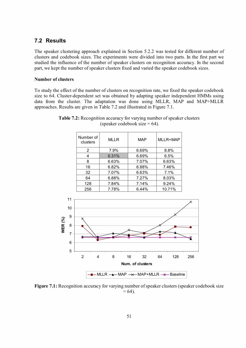
51
7.2 Results
The speaker clustering approach explained in Section 5.2.2 was tested for different number of clusters and codebook sizes. The experiments were divided into two parts. In the first part we studied the influence of the number of speaker clusters on recognition accuracy. In the second part, we kept the number of speaker clusters fixed and varied the speaker codebook sizes. Number of clusters To study the effect of the number of clusters on recognition rate, we fixed the speaker codebook size to 64. Cluster-dependent set was obtained by adapting speaker independent HMMs using data from the cluster. The adaptation was done using MLLR, MAP and MAP+MLLR approaches. Results are given in Table 7.2 and illustrated in Figure 7.1.
Table 7.2: Recognition accuracy for varying number of speaker clusters (speaker codebook size = 64).
Number of clusters MLLR MAP MLLR+MAP
2 7.9% 6.69% 8.8% 4 6.31% 6.69% 6.5% 8 6.63% 7.07% 6.63%
16 6.82% 6.88% 7.46% 32 7.07% 6.63% 7.1% 64 6.88% 7.27% 8.03% 128 7.84% 7.14% 9.24% 256 7.78% 6.44% 10.71%
5
6
7
8
9
10
11
2 4 8 16 32 64 128 256
Num. of clusters
WER
(%)
MLLR MAP MAP+MLLR Baseline
Figure 7.1: Recognition accuracy for varying number of speaker clusters (speaker codebook size = 64).

52
For 4 - 32 clusters, the accuracy is close to the baseline results and for 2, 128 and 256 clusters, MLLR and MAP+MLLR are inferior to baseline. For 4 clusters, MAP reduced WER from 6.63% to 6.31%. Codebook size Next, we varied the speaker codebook size from 4 to 256 and kept the number of speaker clusters fixed to 4. Methods for obtaining cluster dependent HMM sets were kept the same as in the previous test. The results are shown in Table 7.3 and illustrated in Figure 7.2
Table 7.3: Recognition accuracy for varying codebook size (number of speaker clusters = 4).
Speaker codebook
size MLLR MAP MLLR+MAP
4 7.01% 6.82% 6.82% 8 6.44% 6.18% 6.63% 16 6.69% 6.69% 6.76% 32 6.44% 6.63% 6.37% 64 6.31% 6.69% 6.5%
128 6.76% 6.44% 6.37% 256 6.37% 6.5% 6.37%
6
6,2
6,4
6,6
6,8
7
7,2
4 8 16 32 64 128 256
Codebook size
WER
(%)
MLLR MAP MLLR+MAP Baseline
Figure 7.2: Recognition accuracy for varying codebook size (number of speaker clusters = 4).
The best result of 6.18% WER was obtained in the case of MAP adaptation and codebook size equal to 8, i.e. it gave 6.8% relative WER reduction compare to the baseline.
7.3 Discussion
From the first experimental part we can see that in general clustering does not improve accuracy. The best result obtained was about 5% relative WER reduction. For the case of 2 clusters, we repeated the metaclustering algorithm ten times. We found out that in six cases it assigned almost all speakers in a single cluster. The smallest mean squared error was obtained in one of those six

53
cases. The clustering approach is based on suboptimal k-means algorithm, which strongly depends on initial solution. This explains why partitions differ from each other between repetitions. Clustering was tested on an artificial data composed of 2-dimensional vectors and it showed reasonable cluster distribution (see Figure 7.3). It allows concluding that there are no two clear speaker groups in the test set. This effect disappeared when number of clusters was increased.
Figure 7.3: Metaclustering tested on 2D artificial data for the case of two clusters.
We can conclude from Figure 7.2 that the codebook size does not have much effect on recognition results. The only exception is codebook with the size of 4, for which the WER obtained is 7.01%. This can be explained by poor speaker representation. It is quite interesting to analyze the data assigned to each cluster. The division into 4 clusters in a case of codebook size 8 is shown in Figure 7.4.
020406080
100120140160180
1 2 3 4
Cluster num ber
male female
Figure 7.4: Male/female division in a case of 4 clusters and codebook size of 8. In this case the metaclustering algorithm divides speakers into male/female groups with almost 100% probability. This is even more interesting when we compare the results obtained for 2 clusters mentioned above.

54
8 CONCLUSIONS In this thesis, we first studied the theoretical background of speech recognition, considering feature extraction steps along with acoustic modeling issues. After that, we discussed two ways of involving speaker information into speech recognition task: adaptation and clustering. Two classical adaptation approaches, MAP and MLLR, were outlined. Speaker grouping was attacked from different directions. First, we discussed tree-based and plain hard clustering as well as eigenvoices and vocal tract based grouping. The next step of considering speaker in speech recognition was to examine how speaker identification techniques can contribute to our task. Two methods of combining speech and speaker recognition were studied, which approached us to the proposed clustering algorithm. The proposed speaker grouping method clusters speaker codebooks obtained via VQ based speaker modeling. We first trained speaker models with size of 64 using TIMIT training data. After that we applied clustering algorithm to them and obtained different number of clusters. The cluster dependent HMM sets were created by adapting speaker independent models, using the data assigned to each cluster. After that, using speaker identification techniques, we mapped each sentence from the test set to some cluster and used models from that cluster for evaluation. We obtained 5% WER reduction for 4 clusters. Next, we addressed the effect of codebook size. The best result of 6.8% WER reduction compared to the baseline was obtained for the codebook size of 8. We also examined the clusters’ content in the best case and found out that gender separation among clusters was almost 100%. We did not observe dependency between number of clusters and recognition performance. However, for more than 64 clusters, MLLR showed performance degradation. Small codebooks with the size of 4 also turned out to give high error rate due to poor speaker representation. Speaker clustering itself can be also considered as a kind of speaker adaptation where HMM parameters are not changed, but “the best” model set is found. VQ speaker representation provides us with the fast speaker identification process and hence allows adapting speaker recognition system rapidly. Combining speech and speaker recognition can be extended further. First, shifting from hard clustering to the soft one. It requires some weighting function to measure the contribution of every cluster-dependent model set in recognition. An interesting testing would be a comparison of different cluster selection approaches. I.e. it is interesting to find out how different results likelihood-based and matching-based selection strategies would show. In this work we considered speech recognition improvement using speaker recognition. A particularly interesting would be to do the other way round, i.e. to improve speaker identification/verification involving speech recognition.

55
REFERENCES
[1] S. M. Ahadi and P.C Woodland, “Combined Bayesian and Predictive Techniques for Rapid Speaker Adaptation of Continuous Density Hidden Markov Models”. Computer Speech and Language, vol. 11, no. 3, pp. 187-206, 1997.
[2] B. S. Atal, “Effectiveness of Linear Prediction Characteristics of the Speech Wave for Automatic Speaker Identification and Verification”. Journal of the Acoustic Society of America vol. 55, no. 6, pp. 1304-1312, 1974.
[3] J.A. Bilmes, “A Gentle Tutorial of the EM Algorithm and its Applications to Parameter Estimation for Gaussian Mixture and Hidden Markov Models”. Technical report, International Computer Science Institute, Berkeley CA, 1998.
[4] J. P. Campbell, “Speaker Recognition: a Tutorial”. In Proc. of the IEEE, vol. 85, no. 9, pp. 1437- 1462, 1997.
[5] J.-C. Chen, J.-L. Lo and J.-S. Roger Jang, “Computer Assisted Spoken English Learning for Chinese in Taiwan”. International Symposium on Chinese Spoken Language Processing (ISCSLP), Hong Kong, 2004.
[6] J.R Deller, J.H.L. Hansen and J.G. Proakis, ”Discrete–Time Processing of Speech Signals”. IEEE Press, 2nd edition, New York, 2000.
[7] V. Digalakis, S. Tsakalidis, C. Harizakis and L. Neumeyer, “Efficient Speech Recognition Using Subvector Quantization and Discrete-Mixture HMMs”. Computer Speech and Language, no. 14, pp. 33-46, 2000.
[8] P. Faltlhauser and G. Ruske, “Robust Speaker Clustering in Eigenspace”. In Proc. ASRU2001, pp. 57-60, 2001.
[9] G.A. Fink and T. Plötz, “Integrating Speaker Identification and Learning With Adaptive Speech Recognition”. In ODYS, pp. 185-192, 2004.
[10] P. Fränti and J. Kivijärvi, “Randomized Local Search Algorithm for the Clustering Problem”. Pattern analysis and Applications, vol. 3, no. 4, pp. 358-369, 2000.
[11] S. Furui, “Digital Speech Processing, Synthesis, and Recognition”. Marcel Dekker, 2nd edition, New York, 2001.
[12] M. J. F. Gales, “Cluster Adaptive Training of Hidden Markov Models”. IEEE Transactions on Speech and Audio Processing, vol. 8, no. 4, pp. 417-428, 2000.
[13] J.-L. Gauvain and C.-H. Lee, “Maximum a Posteriori Estimation for Multivariate Gaussian Mixture Observations of Markov Chains”. IEEE Transactions on speech and audio processing, vol. 2, pp. 291-298, 1994.
[14] J. Harrington and S. Cassidy. “Techniques in Speech Acoustics”. Kluwer Academic Publishers, Dordrecht, 1999.

56
[15] Haskins Laboratories, WWW page. http://www.haskins.yale.eduhaskins/ EADS/MMSP/ acoustic.html (last visit 03.03.2005).
[16] T. J. Hazen, ”A Comparison of Novel Techniques for Rapid Speaker Adaptation”. Speech Communication, vol. 31, no. 1, pp. 15-33, 2000.
[17] L.P. Heck and D. Genoud, “Combining Speaker and Speech Recognition Systems”. In Proc. International Conference on Spoken Language Processing, pp. 1369-1372, 2002.
[18] X. Huang, A. Acero and H.-W. Hon, “Spoken Language Processing”. Prentice-Hall, Upper Saddle River, New Jersey, USA, 2001.
[19] C. Huang, T. Chen and E. Chang, "Adaptive Model Combination For Dynamic Speaker Selection Training". In Proc. International Conference on Spoken Language Processing, pp. 65-68, 2002.
[20] E. Karpov, T. Kinnunen and P. Fränti, "Symmetric Distortion Measure for Speaker Recognition". In Proc. 9th International Conference Speech and Computer (SPECOM'2004), pp. 366-370, 2004.
[21] T. Kinnunen, “Spectral Features for Automatic Text-Independent Speaker Recognition”. Licentiate’s thesis, University of Joensuu, 2003.
[22] T. Kinnunen, T. Kilpeläinen and P. Fränti, “Comparison of Clustering Algorithms in Speaker Identification”. In Proc. IASTED International Conference Signal Processing and Communications, pp. 222-227, 2000.
[23] T. Kinnunen and Ismo Kärkkäinen, “Class-Discriminative Weighted Distortion Measure for VQ-based Speaker Identification”. International Workshop on Structural and Syntactic Pattern Recognition (SSPR), pp. 681-688, 2002.
[24] T. Kosaka, S. Matsunaga and S. Sagayama, “Speaker-Independent Speech Recognition Based on Tree-Structured Speaker Clustering”. Computer Speech and Language, vol. 10, no. 1, pp. 55-74, 1996.
[25] R. Kuhn, J.-C. Junqua, P. Ngyuen and N. Niedzielski, “Rapid Speaker Adaptation in Eigenvoice Space”. IEEE Transactions on Speech and Audio Processing, vol. 8, no. 6, pp. 695-707, November 2000.
[26] R. Kuhn, F. Perronnin and J.-C. Junqua, “Time is Money: Why Very Rapid Adaptation Matters”. In Adaptation-2001, pp. 33-36, 2001.
[27] C.J. Leggeter and P.C. Woodland, “Speaker Adaptation of HMMs Using Linear Regression”. Technical report, Cambridge University Engineering Department, 1994.
[28] C. J. Leggetter and P. C. Woodland, “Flexible Speaker Adaptation Using Maximum Likelihood Linear Regression”. In Proc. ARPA Spoken Language Technology Workshop, pp. 104-109, February 1995.
[29] Y. Linde, A. Buzo and R. M. Gray, “An Algorithm for Vector Quantizer Design”. IEEE Transactions on Communications, vol. 28, no. 1, 1980.

57
[30] Linguistic data consortium, WWW page. http://www.ldc.upenn.edu/ (last visit 01.03.2005).
[31] M. Naito, L. Deng and Y. Sagisaka, “Speaker Clustering for Speech Recognition Using Vocal-Tract Parameters”. Speech Communication, vol. 36, no. 3, pp. 305-315, 2002.
[32] J. J. Odell, “The Use of Context in Large Vocabulary Speech Recognition”. PhD thesis, Queens’ College, Cambridge, 1995.
[33] L.R. Rabiner, “A Tutorial on Hidden Markov Model and Selected Applications in Speech Recognition”. In Proc. of the IEEE, vol. 77, no. 2, pp. 257-286, 1989.
[34] L.R. Rabiner and B.W. Juang, “Fundamentals of Speech Recognition”. Prentice-Hall, Englewood Cliffs, NJ, USA, 1993.
[35] D. Reynolds and R. Rose, “Robust Text-Independent Speaker Identification Using Gaussian Mixture Speaker Models”. IEEE Transactions on Speech and Audio Processing, vol. 3, no. 1, pp. 72-83, 1995.
[36] A. Sankar, F. Beaufays and V. Digalakis, “Training Data Clustering for Improved Speech Recognition”. In Proc. of the European Conference on Speech Communication and Technology, vol. 1, no. 2, pp. 503-506, 1995.
[37] M. N. Stuttle, “A Gaussian Mixture Model Spectral Representation for Speech Recognition”, Ph.D thesis, Department of Engineering, University of Cambridge, 2003.
[38] Summer Institute of Linguistics, glossary of linguistic terms, WWW page. http://www.sil. org/linguistics/glossaryoflinguisticterms/ (last visit 01.03.2005).
[39] The CMU Pronouncing Dictionary, WWW page. http://www.speech.cs.cmu.edu/cgi-bin/cmudict?in=C+M+U+Dictionary (last visit 01.03.2005).
[40] E. Trentin and M. Gori, “A Survey of Hybrid ANN/HMM Models for Automatic Speech Recognition”. Neurocomputing, vol. 37, pp. 91-126, 2001.
[41] R. Vergin, A. Farhat and D. O’Shaughnessy, “Robust Gender-Dependent Acoustic-Phonetic Modeling in Continuous Speech Recognition Based on a New Automatic Male/Female Classification”. In Proc. International Conference on Spoken Language, vol. 2, pp. 1081-1084, 1996.
[42] P. C. Woodland, “Speaker Adaptation: Techniques and Challenges”. In Proc. IEEE International Workshop on Automatic Speech Recognition and Understanding, pp. 85-90, 1999.
[43] S. Young, J. Jansen, D. Ollason and P. Woodland, “The HTK Book (for HTK version 3.2)”. Cambridge University Engineering Department, 2001.
[44] S. J. Young, J. J. Odell and P.C. Woodland, ”Tying for High Accuracy Acoustic Modeling”. In Proc. ARPA Human Language Technology Conference, Plainsboro, 1994.

58
[45] S. J. Young, N. H. Russell and J. H. S. Thornton, “Token Passing: a Simple Conceptual Model for Connected Speech Recognition Systems”. Technical report, Cambridge University Engineering Department, 1989.

59
Appendix A
Vector quantization (VQ)
Vector quantization (VQ) [29] is a popular source coding technique. It aims to represent a continuous space by a discrete symbols. Let x be a k-dimensional vector whose components are real-valued random values. A vector quantizer maps (quantizes) vector x to another k-dimensional vector y so: )q( xy = , (B.1) where q(⋅) is a quantization operator. A finite set of vectors Y={yi, 1<i<M} is referred to as a codebook and each vector yi is a codevector. The size of the codebook, M, is called the number of partitions or levels in the codebook. VQ requires two main things to be defined:
• Distance measure • Codebook.
While performing quantization an input vector is mapped against each codevector, and the closest one is chosen. In order to measure such closeness, we need to define a distortion (or distance) measure d(x, yi). Using this notation, we can write that vector x is mapped to codevector yi if and only if i=argmin(d(x, yj)). Usually a sum of squared errors is used [18]:
∑=
−=K
iii yx
1
2)(),d( yx , (B.2)
where K is a vector dimension. Another distance measure is Mahalanobis distance and it is defined as follows: )()(),d( 1 yxΣyxyx −−= − , (B.3) where Σ-1 denotes inverse covariance matrix of y. The design of codebook is a NP-hard problem, i.e. there is no way to find an optimal solution in polynomial time. Thus, all algorithms suggest suboptimal solution only. A popular algorithm is the k-means algorithm. K-means clustering
K-means is an iterative clustering algorithm for codebook design. Its goal is to minimize an objective function, given by the equation B.4:
j

60
∑ ∑= ∈
=M
j jjf
1
2)Cx
y-(x , (B.4)
where M is a codebook size, Cj is a j-th partition and yj is a centroid of this partition. Suppose we are given a vector set X and a required number of clusters N. The k-means algorithm consists of the following four steps [11]: 1. Initialization
Randomly select N initial codevectors y1, y2… yN. An initial codebook can be also given as an algorithm input. Set m=0, where m is an iteration variable.
2. Classification Classify every vector x from X into the nearest cluster according to the rule: x ∈ Ci(m) iff d(x,yi(m))< d(x,yj(m)) for all j≠ i, 1≤j,i≤N.
3. Codebook updating Update every codevector computing the centroid of every cluster Ci(m). yi=centroid(Ci(m)), 1≤ i≤N. Set m=m+1.
4. Termination If an objective function value falls below a predefined threshold or codebook does not change, terminate algorithm, otherwise go to the step 2.

61
Appendix B
Phoneme mapping
The mapping from the 45-phone set of the TIMIT to the 39-phone set of the CMU dictionary is shown in Table B.1. In [5] the mapping was applied to 60-phone set used in TIMIT transcriptions. However, these transcriptions (i.e. phone-boundary information) were not used in this work and Table B.1 represents the mapping of those phonemes only which are used in TIMIT lexicon.
Table B.1: Phone mapping from 45 to 39-phone set.
Original phone New phone ax ah axr er ix ih el ah l
em ah m en ah n
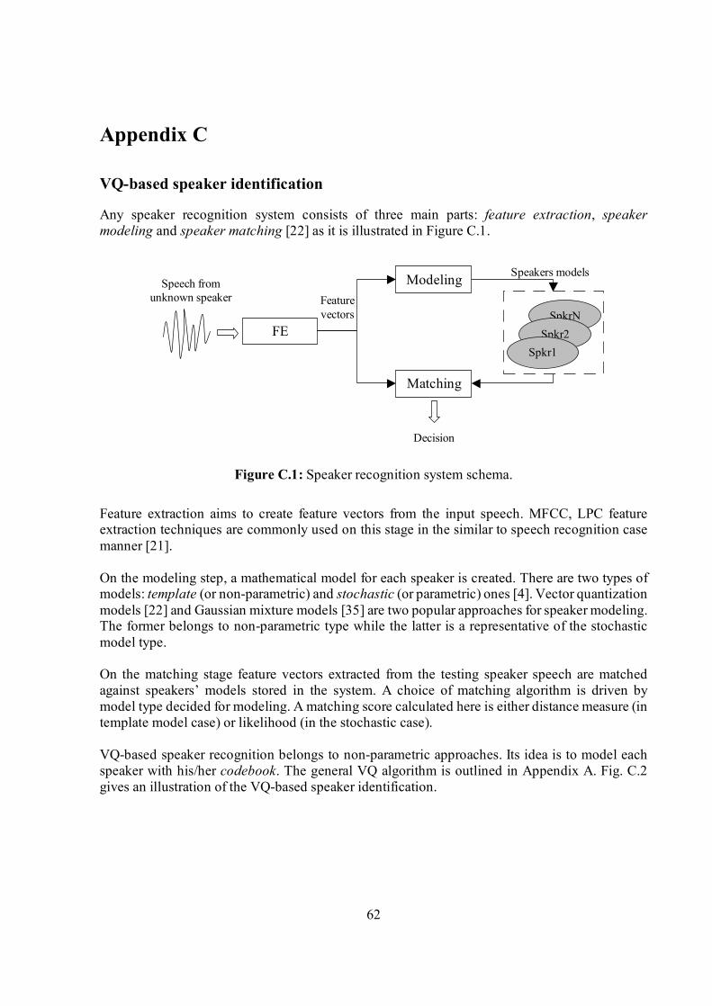
62
Appendix C
VQ-based speaker identification
Any speaker recognition system consists of three main parts: feature extraction, speaker modeling and speaker matching [22] as it is illustrated in Figure C.1.
Figure C.1: Speaker recognition system schema.
Feature extraction aims to create feature vectors from the input speech. MFCC, LPC feature extraction techniques are commonly used on this stage in the similar to speech recognition case manner [21]. On the modeling step, a mathematical model for each speaker is created. There are two types of models: template (or non-parametric) and stochastic (or parametric) ones [4]. Vector quantization models [22] and Gaussian mixture models [35] are two popular approaches for speaker modeling. The former belongs to non-parametric type while the latter is a representative of the stochastic model type. On the matching stage feature vectors extracted from the testing speaker speech are matched against speakers’ models stored in the system. A choice of matching algorithm is driven by model type decided for modeling. A matching score calculated here is either distance measure (in template model case) or likelihood (in the stochastic case). VQ-based speaker recognition belongs to non-parametric approaches. Its idea is to model each speaker with his/her codebook. The general VQ algorithm is outlined in Appendix A. Fig. C.2 gives an illustration of the VQ-based speaker identification.
Speakers models
FE
Modeling
Matching
SpkrN Spkr2
Spkr1
Decision
Speech from unknown speaker Feature
vectors
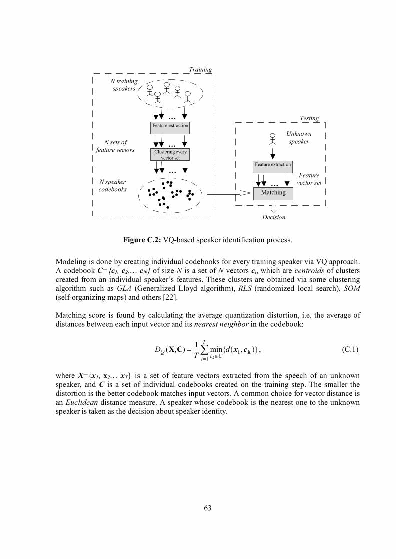
63
Figure C.2: VQ-based speaker identification process.
Modeling is done by creating individual codebooks for every training speaker via VQ approach. A codebook C={c1, c2,… cN} of size N is a set of N vectors ci, which are centroids of clusters created from an individual speaker’s features. These clusters are obtained via some clustering algorithm such as GLA (Generalized Lloyd algorithm), RLS (randomized local search), SOM (self-organizing maps) and others [22]. Matching score is found by calculating the average quantization distortion, i.e. the average of distances between each input vector and its nearest neighbor in the codebook:
∑= ∈
=T
i CcQ d
TD
k1)},({min1),( kiCX cx , (C.1)
where X={x1, x2… xT} is a set of feature vectors extracted from the speech of an unknown speaker, and C is a set of individual codebooks created on the training step. The smaller the distortion is the better codebook matches input vectors. A common choice for vector distance is an Euclidean distance measure. A speaker whose codebook is the nearest one to the unknown speaker is taken as the decision about speaker identity.
Testing
N speaker codebooks
Decision Begin
Feature extraction
Training
Clustering every vector set
…
Unknown speaker
Feature extraction
Matching …
Feature vector set
N sets of feature vectors
N training speakers
…
…