Embed Size (px)
Citation preview

dfgdfg
Special Function Aspects of Macdonald Polynomial Theory
Wendy Catherine Baratta
Submitted in total fulfilment of the requirements
of the degree of Doctor of Philosophy
April, 2011
Department of Mathematics and Statistics
The University of Melbourne

sdsdf

Dedicated to my Grandpa
stuff
stuff
stuff
stuff
stuff
stuff
stuff
stuff
i

ii

Abstract
The nonsymmetric Macdonald polynomials generalise the symmetric Macdonald polyno-
mials and the nonsymmetric Jack polynomials. Consequently results obtained in nonsym-
metric Macdonald polynomial theory specialise to analogous results in the theory of these
other polynomials. The converse, however, does not always apply. Thus some properties
of symmetric Macdonald, and nonsymmetric Jack, polynomials have no known nonsym-
metric Macdonald polynomial analogues in the existing literature. Such examples are
contained in the theory of Jack polynomials with prescribed symmetry and the study of
the Pieri-type formulas for the symmetric Macdonald polynomials. The study of Jack
polynomials with prescribed symmetry considers a special class of Jack polynomials that
are symmetric with respect to some variables and antisymmetric with respect to others.
The Pieri-type formulas provide the branching coefficients for the expansion of the prod-
uct of an elementary symmetric function and a symmetric Macdonald polynomial. In this
thesis we generalise both studies to the theory of nonsymmetric Macdonald polynomials.
In relation to the Macdonald polynomials with prescribed symmetry, we use our new
results to prove a special case of a constant term conjecture posed in the late 1990s. A
highlight of our study of Pieri-type formulas is the development of an alternative viewpoint
to the existing literature on nonsymmetric interpolation Macdonald polynomials. This
allows for greater extensions, and more simplified derivations, than otherwise would be
possible. As a consequence of obtaining the Pieri-type formulas we are able to deduce
explicit formulas for the related generalised binomial coefficients.
A feature of the various polynomials studied within this thesis is that they allow for
explicit computation. Having this knowledge provides an opportunity to experimentally
seek new properties, and to check our working in some of the analytic work. In the last
chapter a computer software program that was developed for these purposes is detailed.
iii

iv

Declaration
This is to certify that
1. The thesis comprises only my original work towards the PhD except where indicated
in the Preface.
2. Due acknowledgement has been made in the text to all other material used.
3. The thesis is less than 100, 000 words in length, exclusive of tables, maps, bibliogra-
phies and appendices.
Wendy Catherine Baratta
v

vi

Acknowldgements
This thesis is the result of constant support and encouragement from my family, friends and
teachers. I thank my grandpa John McInneny for planting the seed from which this thesis
grew. I thank my parents Ross and Linda for providing me with so many opportunities
to enhance and further my education. I thank my high school maths teacher Mary Oswell
for five years of hard, but extremely beneficial work. I thank my university maths lecturer
Maria Athanassenas for sharing her love and enthusiasm for maths, and inspiring me to
do the same. I thank my friend Sam Blake for teaching me Mathematica and consequently
adding a new dimension to my research. I thank my mathematical colleagues Jan De Gier,
Alain Lascoux and Ole Warnaar for interesting discussion and helpful comments. I thank
my career counsellor Ian Wanless for many years of thoughtful advice. I thank my close
family friend Eileen Hannagan for enhancing my PhD experience by making it possible
for me to live closer to the University of Melbourne. I thank my financiers the Australian
Government, the ARC and The University of Melbourne.
To my supervisor Professor Peter Forrester I extend my most earnest thanks. For
three years Peter provided me with fruitful research projects, enthusiastic encouragement
(the always uplifting “wacko”), prompt and regular feedback, much appreciated teaching
experiences, beneficial and enjoyable discussions, skill building tasks and the most valuable
commodity of all, his time. Thank you Peter.
vii

viii

Contents
1 Introduction . . . . . . . . . . . . . . . . . . . . . . . . . . . . . . . . . . . . 1
1.1 A Brief History . . . . . . . . . . . . . . . . . . . . . . . . . . . . . . . . . . 1
1.2 Symmetric Polynomials . . . . . . . . . . . . . . . . . . . . . . . . . . . . . 3
1.2.1 Preliminaries . . . . . . . . . . . . . . . . . . . . . . . . . . . . . . . 3
1.2.2 Some special symmetric polynomials . . . . . . . . . . . . . . . . . . 10
1.3 Nonsymmetric Polynomials . . . . . . . . . . . . . . . . . . . . . . . . . . . 16
1.3.1 Preliminaries . . . . . . . . . . . . . . . . . . . . . . . . . . . . . . . 16
1.3.2 Some special nonsymmetric polynomials . . . . . . . . . . . . . . . . 22
1.4 Interpolation Polynomials . . . . . . . . . . . . . . . . . . . . . . . . . . . . 24
1.4.1 Preliminaries . . . . . . . . . . . . . . . . . . . . . . . . . . . . . . . 24
1.4.2 Some special nonsymmetric interpolation polynomials . . . . . . . . 27
2 Foundational Theory . . . . . . . . . . . . . . . . . . . . . . . . . . . . . . . 31
2.1 Nonsymmetric Macdonald Polynomials . . . . . . . . . . . . . . . . . . . . . 31
2.1.1 Introduction . . . . . . . . . . . . . . . . . . . . . . . . . . . . . . . 31
2.1.2 The eigenopertors . . . . . . . . . . . . . . . . . . . . . . . . . . . . 32
2.1.3 Recursive generation . . . . . . . . . . . . . . . . . . . . . . . . . . . 36
2.1.4 Rodrigues formula . . . . . . . . . . . . . . . . . . . . . . . . . . . . 37
2.1.5 Orthogonality . . . . . . . . . . . . . . . . . . . . . . . . . . . . . . 39
2.1.6 Evaluation formula . . . . . . . . . . . . . . . . . . . . . . . . . . . . 40
2.1.7 A Cauchy formula . . . . . . . . . . . . . . . . . . . . . . . . . . . . 41
2.2 Nonsymmetric Interpolation Macdonald Polynomials . . . . . . . . . . . . . 42
2.2.1 Introduction . . . . . . . . . . . . . . . . . . . . . . . . . . . . . . . 42
2.2.2 The vanishing condition . . . . . . . . . . . . . . . . . . . . . . . . . 43
2.2.3 The eigenoperators . . . . . . . . . . . . . . . . . . . . . . . . . . . . 44
2.2.4 Recursive generation . . . . . . . . . . . . . . . . . . . . . . . . . . . 47
2.2.5 Rodrigues formula . . . . . . . . . . . . . . . . . . . . . . . . . . . . 50
ix

2.2.6 Evaluation formula . . . . . . . . . . . . . . . . . . . . . . . . . . . . 50
2.2.7 The extra vanishing theorem . . . . . . . . . . . . . . . . . . . . . . 52
2.2.8 Binomial coefficients . . . . . . . . . . . . . . . . . . . . . . . . . . . 53
3 Macdonald Polynomials with Prescribed Symmetry . . . . . . . . . . . 55
3.1 A Brief History . . . . . . . . . . . . . . . . . . . . . . . . . . . . . . . . . . 56
3.2 Preliminaries . . . . . . . . . . . . . . . . . . . . . . . . . . . . . . . . . . . 56
3.2.1 Symmetrisation . . . . . . . . . . . . . . . . . . . . . . . . . . . . . . 56
3.2.2 Prescribed symmetry operator . . . . . . . . . . . . . . . . . . . . . 57
3.2.3 The polynomial S(I,J)η∗ (z) . . . . . . . . . . . . . . . . . . . . . . . . 58
3.3 Antisymmetric Macdonald Polynomials . . . . . . . . . . . . . . . . . . . . 63
3.4 Prescribed Symmetry Macdonald Polynomials
with Staircase Components . . . . . . . . . . . . . . . . . . . . . . . . . . . 67
3.4.1 Special form with η∗ = η(n0;Np) . . . . . . . . . . . . . . . . . . . . . 69
3.4.2 Special form with η∗ = η(Np;n0) . . . . . . . . . . . . . . . . . . . . . 70
3.5 The Inner Product of Prescribed Symmetry Polynomials and Constant
Term Identities . . . . . . . . . . . . . . . . . . . . . . . . . . . . . . . . . . 73
3.5.1 The inner product of prescribed symmetry polynomials . . . . . . . 73
3.5.2 Special cases of the prescribed symmetry inner product . . . . . . . 75
3.5.3 The constant term identities . . . . . . . . . . . . . . . . . . . . . . 77
3.6 Further Work . . . . . . . . . . . . . . . . . . . . . . . . . . . . . . . . . . . 83
4 Pieri-Type Formulas for Nonsymmetric Macdonald Polynomials . . . 85
4.1 A Brief History . . . . . . . . . . . . . . . . . . . . . . . . . . . . . . . . . . 86
4.2 Preliminaries . . . . . . . . . . . . . . . . . . . . . . . . . . . . . . . . . . . 87
4.2.1 General Pieri-type formulas . . . . . . . . . . . . . . . . . . . . . . . 87
4.2.2 Structure of Pieri-type expansions . . . . . . . . . . . . . . . . . . . 88
4.3 Pieri-type Formulas for r = 1 . . . . . . . . . . . . . . . . . . . . . . . . . . 90
4.3.1 Non-zero coefficients . . . . . . . . . . . . . . . . . . . . . . . . . . . 91
4.3.2 The intertwining formula . . . . . . . . . . . . . . . . . . . . . . . . 92
4.3.3 The product ziEη . . . . . . . . . . . . . . . . . . . . . . . . . . . . 93
4.3.4 The main result . . . . . . . . . . . . . . . . . . . . . . . . . . . . . 98
4.3.5 The classical limit . . . . . . . . . . . . . . . . . . . . . . . . . . . . 98
4.3.6 Pieri-type formula for r = 1 and the generalised binomial coefficient 100
4.3.7 The Pieri-type formula for r = n− 1 . . . . . . . . . . . . . . . . . . 102
x

4.3.8 Lascoux’s derivation of the Pieri-type formula for r = 1 . . . . . . . 105
4.4 The General Pieri-Type Formulas . . . . . . . . . . . . . . . . . . . . . . . . 107
4.4.1 An alternative derivation of the Pieri-type formulas for r = 1 . . . . 107
4.4.2 The general Pieri-type formula coefficients . . . . . . . . . . . . . . . 111
4.4.3 Simplifying the Pieri coefficients . . . . . . . . . . . . . . . . . . . . 114
4.4.4 Reclaiming the symmetric Macdonald Pieri formulas . . . . . . . . . 115
4.5 Further Work . . . . . . . . . . . . . . . . . . . . . . . . . . . . . . . . . . . 116
5 Computer Programming . . . . . . . . . . . . . . . . . . . . . . . . . . . . . 117
5.1 A Brief History . . . . . . . . . . . . . . . . . . . . . . . . . . . . . . . . . . 117
5.2 Preliminaries . . . . . . . . . . . . . . . . . . . . . . . . . . . . . . . . . . . 118
5.2.1 Recursively generating compositions . . . . . . . . . . . . . . . . . . 118
5.3 Recursively generating polynomials . . . . . . . . . . . . . . . . . . . . . . . 121
5.4 Runtimes and Software . . . . . . . . . . . . . . . . . . . . . . . . . . . . . . 123
5.4.1 Algorithm runtimes . . . . . . . . . . . . . . . . . . . . . . . . . . . 123
5.4.2 Mathematica notebook . . . . . . . . . . . . . . . . . . . . . . . . . 124
5.5 Further Work . . . . . . . . . . . . . . . . . . . . . . . . . . . . . . . . . . . 127
Appendix A Some basic q-functions . . . . . . . . . . . . . . . . . . . . . . . 139
Appendix B Symmetric polynomials . . . . . . . . . . . . . . . . . . . . . . . 141
B.1 Triangular structure . . . . . . . . . . . . . . . . . . . . . . . . . . . . . . . 141
B.2 Orthogonality . . . . . . . . . . . . . . . . . . . . . . . . . . . . . . . . . . . 142
B.3 Eigenfunctions . . . . . . . . . . . . . . . . . . . . . . . . . . . . . . . . . . 143
B.4 Examples . . . . . . . . . . . . . . . . . . . . . . . . . . . . . . . . . . . . . 143
Appendix C Nonsymmetric Jack polynomials . . . . . . . . . . . . . . . . . 145
C.1 Special function properties . . . . . . . . . . . . . . . . . . . . . . . . . . . . 145
C.2 Recursive generation formulas . . . . . . . . . . . . . . . . . . . . . . . . . . 145
C.3 Examples . . . . . . . . . . . . . . . . . . . . . . . . . . . . . . . . . . . . . 146
Appendix D Nonsymmetric Interpolation Jack polynomials . . . . . . . . 147
D.1 Special function properties . . . . . . . . . . . . . . . . . . . . . . . . . . . . 147
D.2 Recursive generation formulas . . . . . . . . . . . . . . . . . . . . . . . . . . 147
D.3 Examples . . . . . . . . . . . . . . . . . . . . . . . . . . . . . . . . . . . . . 148
xi

xii

Chapter 1
Introduction
It is the main aim of this chapter to provide motivation and background for the theory
of the nonsymmetric Macdonald polynomials and nonsymmetric interpolation Macdonald
polynomials required for the main studies of the thesis. The nonsymmetric Macdonald
polynomials and nonsymmetric interpolation Macdonald polynomials are generalisations
of older and more established classes of polynomials. We begin with a brief history of the
relevant polynomial theory to motivate the mathematics in the following sections. We use
the historic development to order our remaining sections, first considering the symmetric
polynomials, secondly the nonsymmetric polynomials and lastly the nonsymmetric inter-
polation polynomials. Each section begins with the required preliminary material and
then moves onto specific families highlighting their special function properties. The key
references for each polynomial class are also provided.
1.1 A Brief History
Symmetric functions originated due to their connection with the representation theory
of the symmetric group. However in the last thirty years they have found applications
in combinatorics, mathematical physics and classical analysis. The history of the subject
dates back to the mid-nineteenth century when Jacobi [38] singled out a family of symmet-
ric functions, now called the Schur functions. The functions are named after Issai Schur as
it was he who found the connection between the functions and the representation theory
of the symmetric and general linear groups [70].
A major development occured in the early 1960’s with the work of Hall [33] and Lit-
tlewood [51] who independently found a one-parameter extension of the Schur function,
referred to naturally as the Hall-Littlewood polynomials. It was the work of Green [29]
1

2 1.1
and Macdonald [52] that identified a connection between these polynomials and the rep-
resentation theory of GLn over finite and p-adic fields.
Around the same time the zonal polynomials were introduced independently by James
[39] and Hua [35]. Although like the Schur and Hall-Littlewood polynomials the zonal
polynomials arose from studies in representation theory, the literature is predominantly
focussed on their applications in statistics [20, 75, 62].
Later that decade Henry Jack [36, 37] discovered another one-parameter generalisation
of the Schur functions that was, besides its limiting properties, very different from the Hall-
Littlewood polynomials. The now called Jack polynomial limits to both the Schur and
zonal polynomials, unifying theories that were originally perceived to be disconnected.
Like the zonal polynomials the Jack polynomials have applications in both representation
theory and statistics [39].
It was not until the 1980’s that all polynomial classes were unified. Macdonald identi-
fied a two parameter family of symmetric polynomials, now named Macdonald polynomials
[53], that generalised both the Hall-Littlewood and Jack polynomials. The Hall-Littlewood
polynomials were obtained by setting one of the parameters to zero and the Jack poly-
nomials by limiting both parameters to one. The Macdonald polynomials generalise the
symmetric characters of compact groups. Credit also goes to Kadell who independently
discovered the polynomials through a connection with his studies on the Selberg integral
[41]. More recently another application to pure mathematics of Macdonald polynomials
was found in the studies of the geometry of the Hilbert scheme of points in the plane [31].
Due to their relation with symmetric characters it was quite unexpected when the poly-
nomials naturally gave rise to a family of nonsymmetric polynomials. The nonsymmetric
Macdonald polynomials were first introduced by Cherednik [15], six years after their sym-
metric counterpart. This came about because of the identification of an algebraic structure
referred to as the double affine Hecke algebra. The symmetric Macdonald polynomials
could be obtained from the nonsymmetric Macdonald polynomials via symmetrisation.
Consequently, it was possible to develop the theory of the symmetric polynomials from
that of their nonsymmetric analogues. This approach was found to be simpler and more
accessible than the previous derivations. Furthermore, due to the limiting properties of
the Macdonald polynomials nonsymmetric analogues of the other symmetric polynomial
classes were automatically obtained. Nonsymmetric Macdonald polynomials, although
rather natural in the Macdonald theory, are still somewhat mysterious, as unless some
parameters are specified they do not have a clear representation-theoretic meaning. The

1.2 3
nonsymmetric polynomials have found application in physics in the study of an ideal gas
[32, 72, 7].
The nonsymmetric polynomials were found themselves to be generalisable to the so-
called interpolation polynomials. These were first found independently by Knop [44] and
Sahi [67] in the field of Capelli identities. They were observed to be the inhomogeneous
generalisation of the symmetric and nonsymmetric polynomial classes and were defined by
rather simple vanishing properties. The interpolation polynomials were able to simplify
the derivation of many polynomial properties more significantly than what was done by
the nonsymmetric polynomials.
The definitive reference on symmetric functions and their applications is Macdonald’s
book “Symmetric functions and Hall polynomials” [54]. For further details on the history
of symmetric polynomials, bibliographical notes on the key contributers and reprints of
[51] and [36] we refer the reader to the proceedings of the 2003 workshop on Jack, Hall-
Littlewood and Macdonald polynomials [47].
1.2 Symmetric Polynomials
1.2.1 Preliminaries
In this section we provide the basic properties of permutations and partitions required for
the introduction of the symmetric polynomial classes and their special function properties.
Unless otherwise stated we are following [54].
Permutations and their Decompositions
A permutation of Nn := 1, . . . , n is a bijection σ : Nn → Nn. Commonly we write σ as
the n-tuple σ := (σ(1), . . . , σ(n)). An inversion of a permutation σ is a pair (i, j) where
i < j and σ(i) > σ(j). With Kj(σ) given by
Kj(σ) := # i : (i, j) is an inversion of σ (1.1)
the length of a permutation σ is defined to be
l(σ) :=
n∑
j=1
Kj(σ)
= (i, j) : i < j, σ(i) > σ(j) .

4 1.2
The set of permutations, with multiplication defined by composition, form a group Sn of
size n! called the symmetric group of order n. For example when n = 3 we have
S3 = (1, 2, 3), (2, 1, 3), (1, 3, 2), (2, 3, 1), (3, 1, 2), (3, 2, 1). (1.2)
The transposition sij is a permutation that interchanges the ith and jth components,
defined by
sij(k) :=
j, k = i
i, k = j
k, k 6= i, j.
From this we can introduce the simple transpositions si, i = 1, . . . , n− 1,
si := si,i+1,
which interchanges the positions i and i + 1 in the n-tuple. The simple transpositions
satisfy the algebraic relations
sisi+1si = si+1sisi+1, 1 ≤ i ≤ n− 2
sisj = sjsi, |i− j| > 1 (1.3)
s2i = 1,
the first two of which are referred to as the braid relations. These algebraic relations
generate the symmetric group [59] and therefore any permutation σ ∈ Sn can be written
as a product of simple transpositions. The products of smallest length are referred to as
reduced decompositions and are of length l(σ). A reduced decomposition is denoted by
sσ and given explicitly by
sσ := s1 . . . s2−K2(σ) . . . sn−2 . . . sn−1−Kn−1(σ)sn−1 . . . sn−Kn(σ),
where Kj(σ) is given by (1.1). To avoid unnecessary ambiguity in the interpretation
of the reduced decomposition we state that the product is read from left to right, that
is sσ = si1si2 . . . sil . For example with σ = (3, 2, 4, 1) we have a reduced decomposition
sσ = s1s3s2s1.We note that a reduced decomposition is generally not unique, for example,
another reduced decomposition for σ = (3, 2, 4, 1) is sσ = s3s2s1s2.

1.2 5
The simple transpositions act on functions by interchanging the variables zi and zi+1
(sif)(z1, . . . , zi, zi+1, . . . , zn) := f(z1, . . . , zi+1, zi, . . . , zn).
For example
s2s1f(z1, z2, z3) = s2f(z2, z1, z3) = f(z3, z1, z2).
More generally the action of permutations on polynomials is specified by
sσf(z1, . . . , zn) = sil . . . si2si1f(z1, . . . , zn) = σf(z1, z2, . . . , zn) = f(zσ(1), . . . , zσ(n)).
(1.4)
Throughout this thesis we introduce many operators that are labelled by the integers
1, . . . , n− 1. It is regularly required that these operators act on polynomials in a sequence
specified by a permutation. For example if we have the operators F1, . . . , Fn−1 and a
permutation represented by the reduced decomposition sσ = si1 . . . sil we define
Fσ := Fi1 . . . Fil (1.5)
and specify the action of Fσ on polynomials according to
Fσf(x) = Fil . . . Fi1f(x).
Partitions, diagrams and orderings
The polynomials in this section are labelled by partitions. A partition is defined to be any
(finite or infinite) sequence of non-negative and weakly decreasing integers
κ = (κ1, κ2, . . .), κ1 ≥ κ2 ≥ . . .
containing only finitely many non-zero terms. In this thesis we consider only partitions
containing finitely many integers. Each κi is referred to as a component of κ and the length
of a partition, denoted by n, is defined to be the number of components of κ. We denote
the number of non-zero components of a partition by ℓ(κ). The modulus of a partition is
denoted by |κ| and is equal to the sum of its components. That is, if we take κ = (4, 2, 0)
we have n = 3, ℓ(κ) = 2 and |κ| = 6.
The first ordering we define on partitions is the lexicographic ordering ⋖. The lexi-
cographic ordering compares partitions of the same modulus and is defined by µ ⋖ κ if

6 1.2
the first non-vanishing difference κi − µi is positive. The lexicographic ordering is a total
ordering, meaning all partitions of a particular modulus are comparable. For example, the
partitions of modulus 4 are ordered as
(4, 0, 0, 0), (3, 1, 0, 0), (2, 2, 0, 0), (2, 1, 1, 0), (1, 1, 1, 1).
The second ordering is the dominance ordering. The dominance ordering is an ordering
on partitions of the same modulus and defined by
µ ≤ κ iff Σpi=1(κi − µi) ≥ 0 for all 1 ≤ p ≤ n.
This is only a partial ordering, as for example the partitions (4, 1, 1) and (3, 3, 0) are
incomparable under ≤ .
Each partition κ has a corresponding diagram defined to be the set of points (i, j) ∈ Z2
such that 1 ≤ j ≤ κi, ordered as for a matrix (row 1 along the top). For convenience we
draw the diagram by replacing the elements of Z2 with boxes, the box in the ith row and
jth column is labelled by (i, j). We denote the diagram of a composition κ by diag(κ). For
example, with κ = (11, 8, 8, 7, 5, 4, 2, 2, 1, 1) we have
diag(κ) =
For each box s = (i, j) in a partition κ, the number of boxes to the right, left, below and
above s are the arm length aκ(s), arm colength a′κ(s), leg length lκ(s) and leg colength
l′κ(s), respectively. These are formally defined by
aκ(s) := κi − j, a′κ(s) := a′κ(j) := j − 1, (1.6)
lκ(s) := # k : k > i, j ≤ κk , l′κ(s) := l′κ(i) := i− 1.
For example, if we have the κ defined as above and take the box s = (2, 3) we have

1.2 7
sa′κ(s) = 2 aκ(s) = 5
l′κ(s) = 1
lκ(s) = 4
For two partitions such that µ ⊂ κ we have a skew diagram κ/µ which consists of
those boxes of κ which are not in µ. A skew diagram is said to be a vertical m-strip if κ/µ
consists of m boxes, all of which are in distinct rows. For example, with κ = (4, 3, 1, 1)
and µ = (3, 2, 1), κ/µ is a vertical 3-strip. Pictorially we have
κ/µ =
Symmetric polynomials
We consider the set of polynomials in n independent variables z := (z1, . . . , zn) with
rational integer coefficients, denoted Q[z1, . . . , zn]. Equation (1.4) shows that permutations
act on polynomials by permuting variables. We classify a polynomial as symmetric if it is
invariant under the action of any permutation, that is
sif(z) = f(z), for all i = 1, . . . , n− 1.
For example, the polynomial z1+z2 is considered symmetric if n = 2 but is not symmetric
if n = 3.
As a consequence of this property any symmetric polynomial can be expressed as a
linear combination of eκ(z) := eκ1(z) . . . eκn(z) where eκi(z) are the elementary symmetric
functions defined by
er(z) :=∑
1≤i1<...<ir≤n
zi1 . . . zir .

8 1.2
Other classes of polynomials that are considered to be building blocks of all symmetric
functions are the complete symmetric functions hr(z)
hr(z) :=∑
1≤i1≤...≤ir≤n
zi1 . . . zir , (1.7)
the symmetric monomial functions mκ(z)
mκ(z) :=∑
σ
zσκ, (1.8)
and the power sums pκ(z)
pκ(z) := pκ1(z) . . . pκn(z),
where
pr(z) :=
n∑
i=1
zri = m(r,0,...,0)(z).
We note that the power sums are not linearly independent unless the number of variables
is large enough. In (1.8) the sum is over all distinct permutations σ of κ and zκ denotes
the monomial corresponding to the partition κ and is defined by
zκ := zκ11 . . . zκn
n . (1.9)
The symmetrisation operator
Sym :=∑
σ∈Sn
sσ
can transform any polynomial to a symmetric polynomial. For example, with n = 3
Sym(z1 + z2) =(z1 + z2) + s1(z1 + z2) + s2(z1 + z2)
+ s2s1(z1 + z2) + s1s2(z1 + z2) + s1s2s1(z1 + z2)
=4(z1 + z2 + z3),
a symmetric polynomial in z1, z2 and z3.
Related to the symmetric polynomials are the antisymmetric polynomials. These poly-
nomials change sign upon the interchange of any two variables and hence are defined by
sif(z) = −f(z), for all i = 1, . . . , n− 1.

1.2 9
The antisymmetrisation operator is defined to be
Asym :=∑
σ∈Sn
(−1)l(σ)sσ,
and works in an analogous way to the Sym operator. Furthermore,
Asym f(z) = ∆(z)g(z) (1.10)
where
∆(z) :=∏
i<j
(zi − zj) (1.11)
is the Vandermonde product and g(z) is symmetric.
t-symmetric polynomials
For reasons to be made clear in Chapter 2, t-analogues of Sym and Asym are required.
To construct such operators we first require the t-analogue of si and the definitions of
t-symmetric and t-antisymmetric.
The operators Ti, referred to as the Demazure-Lustig operators, that generalise si are
realisations of the type-A Hecke algebra. The type-A Hecke algebra is an associative unital
algebra over Q(t) generated by elements h1, . . . , hn−1 and subject to the relations
hihi+1hi = hi+1hihi+1, for 1 ≤ i ≤ n− 2
hihj = hjhi, |i− j| > 1 (1.12)
(hi + 1)(hi − t) = 0.
The operators Ti are defined by
Ti := t+tzi − zi+1
zi − zi+1(si − 1). (1.13)
We note that in the limit t→ 1 (1.12) reduces to (1.3) and Ti reduces to si.
From this operator we define a polynomial to be t-symmetric if
Tif (z) = tf (z) , for all i = 1, . . . , n− 1,

10 1.2
and t-antisymmetric if
Tif (z) = −f (z) , for all i = 1, . . . , n− 1.
We note that by the definition of Ti being t-symmetric is an equivalent condition to being
symmetric, consequently when we speak of a symmetric polynomial we are not required
to specify the nature of the symmetry.
The t-analogues of Sym and Asym are given respectively by
U+ :=∑
σ∈Sn
Tσ, (1.14)
and
U− :=∑
σ∈Sn
(−1
t
)l(σ)
Tσ, (1.15)
where the operator Tσ is as in (1.5).
For example, with n = 3
U+(z1 + z2) =(z1 + z2) + T1(z1 + z2) + T2(z1 + z2)
+ T2T1(z1 + z2) + T1T2(z1 + z2) + T1T2T1(z1 + z2)
=(1 + t)2(z1 + z2 + z3),
a t-symmetric polynomial in the variables z1, z2 and z3.
The t-analogue of (1.10) is
U−f(z) = ∆t(z)g(z) (1.16)
where
∆t(z) :=∏
i<j
(zi − t−1zj), (1.17)
is the t-Vandermonde product and g(z) is a symmetric polynomial.
1.2.2 Some special symmetric polynomials
Over the years, various applied and theoretical advances have isolated some special classes
of symmetric polynomials beyond the simple building blocks introduced in the previous
section. These are the Schur polynomials sκ(z), zonal polynomials Zκ(z), Hall-Littlewood
polynomials Pκ(z; t), symmetric Jack polynomials Pκ(z;α) and symmetric Macdonald

1.2 11
polynomials Pκ(z; q, t). As detailed in the following diagram, it turns out that by tak-
ing different limits of the two parameters in the symmetric Macdonald polynomials, we
can obtain all the other special symmetric polynomials just listed.
Pκ(z; q, t)
Pκ(z; t) Pκ(z;α)
sκ(z) Zκ(z)
t = q1/α, q → 1
q = 0
t = 0
α = 1
α = 2
Here we discuss some fundamental properties of the symmetric Macdonald polynomial
Pκ(z; q, t). The corresponding properties of the other special symmetric polynomials follow
by the limits of the diagram. For convenience, the latter are listed in Appendix B along
with the relevant references.
Triangular structure
The symmetric Macdonald polynomials are labelled by a partition κ and have the trian-
gular structure
Pκ(z; q, t) = mκ(z) +∑
µ<κ
Kκµmµ(z), (1.18)
for some coefficients Kκµ ∈ Q(q, t). Since all µ < κ satisfies |µ| = |κ| we also have that
Pκ(z; q, t) is a homogeneous polynomial, meaning each term in the polynomial is of the
same degree.
The following examples highlight the triangular structure of the symmetric Macdonald
polynomials,
P(3,0,0)(z; q, t) = m(3,0,0)(z) +(q2+q+1)(t−1)
q2t−1 m(2,1,0)(z) +(q+1)(q2+q+1)(t−1)2
(qt−1)(q2t−1) m(1,1,1)(z)
P(2,1,0)(z; q, t) = m(2,1,0)(z) +(t−1)(2qt+q+t+2)
qt2−1m(1,1,1)(z) (1.19)
P(1,1,1)(z; q, t) = m(1,1,1)(z).
Eigenfunctions
The symmetric Macdonald polynomials are eigenfunctions of the operator
D1n :=
n∑
i=1
∏
i 6=j
tzi − zjzi − zj
τi, (1.20)

12 1.2
where τi is a q-shift operator and defined by
(τif)(z1, . . . , zi, . . . , zn) := f(z1, . . . , qzi, . . . , zn). (1.21)
Explicitly
D1nPκ(z; q, t) =MκPκ(z; q, t), (1.22)
where Mκ :=∑n
i=1 qκitn−i and is an eigenvalue.
The symmetric Macdonald polynomials can be defined solely by their triangular struc-
ture and eigenfunction properties. This is a consequence of the triangular action of D1n on
the symmetric monomial functions, specified by
D1nmκ(z) =Mκmκ(z) +
∑
µ<κ
Nκµmµ(z), (1.23)
whereMκ is defined above andNκµ ∈ Q(q, t). The eigenfunction property, triangular struc-
ture and the triangular action of the eigenoperator on the monomial functions provides
a user-friendly method for constructing the polynomials. Before providing the details of
this construction we consider one last property of the symmetric Macdonald polynomials.
Orthogonality
A family of polynomials, Fκ say, is said to be orthogonal if there exists an inner product
〈·, ·〉 such that
〈Fκ, Fµ〉 = Lκδκ,µ (1.24)
for some positive constant Lκ. As an inner product 〈·, ·〉 is symmetric, bilinear and positive
definite. In (1.24) δκ,µ is the Kronecker delta and is defined to be 1 if κ = µ and zero
otherwise. Macdonald [54] defines an inner product, of which the symmetric Macdonald
polynomials are orthogonal with respect to, by the power sum orthogonality
〈pκ(z), pµ(z)〉pq,t = δκ,µcκ
ℓ(κ)∏
i=1
1− qκi
1− tκi, (1.25)
where cκ :=∏
i imimi!, with mi := mi(κ) being the number of components in κ equal to
i. The number of variables in the power sums in (1.25) is equal to the maximum of |κ|
and |µ|.

1.2 13
The symmetric Macdonald polynomials are also orthogonal with respect to another
inner product. With zi = e2πixi we introduce the general inner product [14]
〈f, g〉Intq,t =
∫ 1
0dx1 . . .
∫ 1
0dxnf(z; q, t)g(z
−1; q−1, t−1)W (z), (1.26)
whereW (z) is some weight function (defined explicitly in (2.20)). Alternatively, this inner
product can be expressed as
〈f, g〉(CT)q,t = CT(f(z; q, t)g(z−1; q−1, t−1)W (z)), (1.27)
where CT(f) denotes the constant term with respect to z of any Laurent polynomial f(z)
where z ∈ [z1, z−11 , . . . , zn, z
−1n ]. The formula (1.27) is particularly useful when W (z) itself
is a Laurent polynomial.
A concept naturally arising within inner product theory is the notion of an adjoint
operator. We say H∗ is the adjoint operator of H with respect to the inner product 〈·, ·〉 if
〈f,Hg〉 = 〈H∗f, g〉. (1.28)
It is fundamental that D1n is self adjoint with respect to both the inner products (1.26)
and (1.27).
These results lead us to our first theorem.
Theorem 1.2.1. We have
〈Pκ(z; q, t), Pµ(z; q, t)〉pq,t = Lκδκ,µ, (1.29)
for normalisations Lκ ∈ Q(q, t).
Proof. By the eigenfunction properties of the symmetric Macdonald polynomials and the
bilinearity of 〈·, ·〉pq,t we can use the fact that
〈D1nPκ(z; q, t), Pµ(z; q, t)〉
pq,t = 〈Pκ(z; q, t),D
1nPµ(z; q, t)〉
pq,t
to show
(Mκ −Mµ)〈Pκ(z; q, t), Pµ(z; q, t)〉pq,t = 0.

14 1.2
When κ 6= µ, Mκ 6= Mµ and therefore 〈Pκ(z; q, t), Pµ(z; q, t)〉pq,t = 0. Furthermore, it
follows from the definition of 〈·, ·〉pq,t that 〈Pκ(z; q, t), Pκ(z; q, t)〉pq,t 6= 0. These results
together show (1.29) holds true.
The triangular structure and the orthogonality of the symmetric Macdonald polynomi-
als allows the coefficients Kκµ in (1.18) to be constructed recursively by the Gram-Schmidt
process. We provide a detailed description of the construction of P(2,1,0)(z; q, t) in the fol-
lowing section.
Generation
We first show how to generate the general symmetric Macdonald polynomial Pκ(z; q, t)
using the eigenfunction properties.
Suppose we wish to generate the symmetric Macdonald polynomial Pκ(z; q, t) for which
there are k partitions µ, denoted µ1, µ2, . . . , µk, such that µ < κ. From (1.18) we have
Pκ(z; q, t) = mκ(z) +K1mµ1(z) +K2mµ2(z) + . . .+Kkmµk(z), (1.30)
for some coefficients K1, . . . ,Kk ∈ Q(q, t). Acting upon Pκ(z; q, t) with D1n according to
(1.22) gives
D1nPκ(z; q, t) =Mκ(mκ(z) +K1mµ1(z) +K2mµ2(z) + . . . +Kkmµk(z)). (1.31)
Alternatively, using (1.23) we obtain
D1nPκ(z; q, t) =Mκmκ(z) +Nκµ1mµ1(z) +Nκµ2mµ2(z) + . . .+Nκµkmµk(z)
Mκmκ( +K1(Mµ1mµ1(z) +Nµ1µ2mµ2(z) + . . .+Nµ1µkmµk(z))
Mκmκ(z) +Mµ1mµ1(z)+ +K2(Mµ2mµ2(z) + . . .+Nµ2µkmµk(z)) (1.32)
...Mκmκ(+
Mκmκ(z) +Mµ1mµ1(z) +Mµ2mµ2(z) + . . .++Kn(Mµkmµk(z)).

1.2 15
We can represent the sets of equations given in (1.31) and (1.32) as the matrix equation
Mκ Nκµ1 Nκµ2 · · · Nκµk
0 Mµ1 Nµ1µ2 · · · Nµ1µk
0 0 Mµ2 · · · Nµ2µk
......
0 0 0 · · · Mµk
1
K1
K2
...
Kn
=Mκ
1
K1
K2
...
Kn
. (1.33)
It therefore follows that the eigenvector corresponding to eigenvalue Mκ will provide the
coefficients K1, . . . ,Kn in (1.30) giving an explicit formula for Pκ(z; q, t). Moreover, if κ
is chosen to be the highest partition with respect to the partial ordering < the system
(1.33) will have k + 1 eigenvectors, one for each eigenvalue Mκ,Mµ1 , . . . ,Mµk , giving the
coefficients of each of Pκ(z; q, t), Pµ1 (z; q, t), . . . , Pµk(z; q, t).
An alternate method for generating the symmetric Macdonald polynomials is using
their orthogonality properties with respect to 〈·, ·〉pq,t and the Gram-Schmidt procedure. We
first show how one would construct P(2,1,0)(z; q, t) and then describe the general approach.
By the triangular structure of the symmetric Macdonald polynomials we have
P(1,1,1)(z; q, t) = m(1,1,1)(z) and P(2,1,0)(z; q, t) = m(2,1,0)(z) +K(2,1,0),(1,1,1)m(1,1,1)(z).
We can determine the coefficient K(2,1,0),(1,1,1) = K(1,1,1) by solving
〈P(1,1,1)(z; q, t), P(2,1,0)(z; q, t)〉pq,t = 0. (1.34)
To solve the equation we first need to express the symmetric Maconald polynomials in
terms of the power sums. To do this we require the expansions,
m(1,1,1)(z) = (p(1,1,1)(z)− 3p(2,1,0)(z) + 2p(3,0,0)(z))/6
m(2,1,0)(z) = p(2,1,0)(z)− p(3,0,0)(z).
Rewriting P(1,1,1)(z; q, t) and P(2,1,0)(z; q, t) in terms of the power sums allows us to use
the definition of 〈·, ·〉pq,t to simplify (1.34) to
K(1,1,1)(1− q)3
6(1− t)3+
(2−K(1,1,1))(1− q)(1− q2
)
2(1 − t) (1− t2)+
(K(1,1,1) − 3)(1− q3
)
3(1 − t3)= 0.

16 1.3
The solution to this equation is
K(1,1,1) =(t− 1)(2qt+ q + t+ 2)
qt2 − 1,
which is consistent with (1.19).
In the general case one can construct the set of symmetric Macdonald polynomials of
modulus k using the Gram-Schmidt method by first taking P(1k)(z; q, t) and sequentially
generating the polynomials according to the lexicographic order, completing the process
at P(k,0...,0)(z; q, t).
Notes: Further families of symmetric polynomials are the Hermite, Laguerre and Jacobi
polynomials. These families are related to the Jack polynomials but are not directly con-
nected to the Macdonald polynomials. Consequently we do not provide the details of these
polynomials in this thesis. Interested readers can find the details in [23, Chap. 13]. Two
families directly relating to the Macdonald polynomials are the symmetric Al-Salam and
Carlitz polynomials [8]. Both polynomials are defined in terms of the Macdonald polyno-
mials, have eigenfunction properties and form an orthogonal set with respect to an inner
product. Additional applications of the symmetric Jack polynomials are in random matrix
theory and we refer the reader to [17] for an overview of studies in the area.
We also mention that the Schur and Hall-Littlewood polynomials can simply be obtained
using the explicit formulas
sκ(z) :=Asym(zκ+δ)
Asym(zδ)and Pκ(z; t) :=
∏i
1− t
1− tm(i)Sym
(zκ∏
i<j
xi − txjxi − xj
),
where m(i) is defined just below (1.25).
1.3 Nonsymmetric Polynomials
1.3.1 Preliminaries
Here we present the preliminary material on compositions required for the theory of non-
symmetric polynomials. Unless otherwise stated a reference containing the material in
this section is [57].
Compositions, diagrams and orderings
Each nonsymmetric polynomial is labelled by a composition. We define a composition to
be an n-tuple η := (η1, . . . , ηn) of non-negative integers. As with partitions each ηi is called

1.3 17
a component, the length of a composition is the number of components it contains and the
sum of the components is called the modulus and denoted |η|. We define permutations to
act on compositions by
sσ(η1, . . . , ηn) = sil . . . si2si1(η1, . . . , ηn) = σ(η1, . . . , ηn) := (ησ−1(1), . . . , ησ−1(n)). (1.35)
According to this
siση = (ησ−1si(1), . . . , ησ−1si(i), ησ−1si(i+1), . . . , ησ−1si(n))
= (ησ−1(1), . . . , ησ−1(i+1), ησ−1(i), . . . , ησ−1(n))
and thus si acts on compositions by always interchanging the ith and (i+1)th components
regardless of their value. For example
s2s1(η1, η2, η3) = s2(η2, η1, η3) = (η2, η3, η1).
We note that it is the difference between how si acts on polynomials and compositions
that accounts for the variation between (1.4) and (1.35). A further important operator
that acts on compositions is the raising operator Φ which has the action
Φη := (η2, . . . , ηn, η1 + 1).
It is clear that all compositions can be recursively generated from η = (0, . . . , 0) using
the two operators si and Φ. An explanation of a computational approach to generating
any composition most efficiently is given in Chapter 5.
Each composition η corresponds to a unique partition η+ obtained by suitably rear-
ranging the components of η. We define ωη to be the shortest permutation such that
ω−1η (η) = η+. (1.36)
We denote the reverse composition by ηR and the composition where each component is
increased by k by η + (kn), explicitly
ηR := (ηn, ηn−1, . . . , η1) (1.37)
and
η + (kn) := (η1 + k, . . . , ηn + k). (1.38)

18 1.3
There are two important partial orderings on compositions. The dominance ordering
≤ from the previous section and a further ordering . The partial order is defined on
compositions of the same modulus so that
λ η iff λ+ < η+ or in the case λ+ = η+, λ ≤ η. (1.39)
For example two compositions that lie below (0, 1, 2, 1) according to are (0, 1, 1, 2) and
(1, 1, 1, 1).
The diagrams of compositions are defined the same as diagrams for partitions. For
example, with η = (2, 6, 1, 3, 5, 4, 7, 6, 1) we have
diag(η) =
In the previous section we gave formulas for the arm length, arm colegth, leg length and
leg colength of a box in a partition. Sahi [68] generalised these quantities to apply to
compositions. For compositions the definition of arm length and arm colength remain the
same while leg length and leg colength are defined by
lη(s) := # k < i : j ≤ ηk + 1 ≤ ηi+# k > i : j ≤ ηk ≤ ηi
l′η(s) := l′η(i) := # k < i : ηk ≥ ηi+# k > i : ηk > ηi.
(1.40)
For example, for the composition η = (2, 6, 1, 3, 5, 4, 7, 6, 1, 3, 5, 6, 7, 4, 2) and the box s =
(8, 3) we have the diagram

1.3 19
s
showing lη(s) = 8 and l′η(s) = 3.
The concept of a skew diagram is identical for compositions. For example, with η =
(3, 4, 1, 1) and λ = (3, 3, 1), η/λ is a vertical 2-strip. Pictorially we have
η/λ =
Diagram dependent constants
The following quantities
dη := dη(q, t) =∏
s∈diag(η)
(1− qaη(s)+1tlη(s)+1),
d′η := d′η(q, t) =∏
s∈diag(η)
(1− qaη(s)+1tlη(s)), (1.41)
eη := eη(q, t) =∏
s∈diag(η)
(1− qa′η(s)+1tn−l′η(s)) , (1.42)
e′η := e′η(q, t) =∏
s∈diag(η)
(1− qa′η(s)+1tn−1−l′η(s)),
which are constants independent of the polynomial variable z, appear regularly in Mac-
donald polynomial theory. Most important for our studies is knowing how these constants
transform under the action of si and Φ on η. We will first consider the action of si. For
this we require the quantity
δi,η := δi,η(q, t) = ηi/ηi+1. (1.43)

20 1.3
The symbol ηi denotes the eigenvalue of the nonsymmetric Macdonald polynomial and is
defined by ηi := qηit−l′η(i). This quantity plays a crucial role throughout our studies and
will be given a more thorough introduction in Chapter 2.
Lemma 1.3.1. [68] We have
esiη(q, t) = eη(q, t) (1.44)
dsiη(q, t)
dη(q, t)=
1−tδi,η(q,t)1−δi,η(q,t)
, ηi > ηi+1
1−δi,η(q,t)t−δi,η(q,t)
, ηi < ηi+1,
(1.45)
where δi,η(q, t) is given by (1.43).
Proof. Consider first eη(q, t). Taking s = (i, j) we have qa′η(s)+1 = qj and l′η(s) = l′η(i)
allowing (1.42) to be rewritten as
eη(q, t) =n∏
i=1
ηi∏
j=1
(1− qjtn−l′η(i)).
Since siη is a permutation of η, it follows that esiη(q, t) corresponds to a reordering of
terms in (1.3.1) only and thus eη(q, t) = esiη(q, t). In relation to dη(q, t), when ηi > ηi+1,
we must first recognise that switching rows i and i + 1 increases the leg of the point
(i, ηi+1 + 1) by one while all other arms and legs stay the same. Hence,
dsiη(q, t)
dη(q, t)=
1− qaη(s)+1tlη(s)+2
1− qaη(s)+1tlη(s)+1, (1.46)
where s = (i, ηi+1 + 1). We simplify this by observing that for s = (i, ηi+1 + 1) we have
ηi−ηi+1 = aη(s)+1 and l′η(i+1)− l′η(i) = lη(s)+1. The latter is true since with ηi > ηi+1
we have
# k < i+ 1 : ηk ≥ ηi+1 −# k < i : ηk ≥ ηi = # k < i : ηi > ηk ≥ ηi+1+ 1
= #k < i, ηi+1 + 1 ≤ ηk + 1 ≤ ηi+ 1
and
# k > i+ 1 : ηk > ηi+1 −# k > i : ηk > ηi = # k > i : ηi+1 + 1 ≤ ηk ≤ ηi .
Consequently, qaη(s)+1tlη(s)+1 = ηi/ηi+1 = δi,η(q, t). Substituting this into (1.46) gives the
required result. The case where ηi < ηi+1 can be derived immediately from the previous

1.3 21
result by considering the ratio dη(q, t)/dsiη(q, t) where (siη)i > (siη)i+1 and recalling that
δi,siη(q, t) = δ−1i,η (q, t).
The quantities e′η(q, t) and d′η(q, t) have a similar dependence on aη(s) and lη(s) to
eη(q, t) and dη(q, t). Consequently the relations equivalent to (1.44) and (1.45) can be
deduced in an analogous way.
Lemma 1.3.2. [68] We have
e′siη(q, t) =e′η(q, t),
d′siη(q, t)
d′η(q, t)=
1−δi,η(q,t)1−t−1δi,η(q,t)
, ηi > ηi+1
t−1−δi,η(q,t)1−δi,η(q,t)
, ηi < ηi+1.
(1.47)
Consider now the action of Φ.
Lemma 1.3.3. [68] We have
dΦη(q, t)
dη(q, t)= 1− qη1+1tn−l′η(1) =
eΦη(q, t)
eη(q, t). (1.48)
Proof. The diagram of Φη is obtained from η by removing the top row, fixing an additional
box to it, moving it to the bottom row and shifting the entire diagram up one unit. To
show the first equality we consider the new point to be prefixed to the beginning of the
row and so at s = (n, 1). From their definitions (1.6) and (1.40) one sees that the arms
and legs of all other points are unchanged. The new point s has a(s) = η1 and l(s) =
# k < n : 1 ≤ (Φη)k + 1 ≤ η1 + 1 . By observing that (Φη)k = ηk+1 for k = 1, . . . , n− 1
we can rewrite l(s) as l(s) = # k > 1 : ηk ≤ η1 = n− 1− l′(s) which gives the required
result. For the second equality we consider the new point to be appended to the end of
the row and so at s = (n, η1 +1). This time the coarms and the colegs of the other points
are unchanged and for the new point s we have a′(s) = η1 and l′(s) = # k > 1 : ηk > η1
and the result follows.
As before we state the results equivalent to (1.48) for e′η(q, t) and d′η(q, t) seperately.
Lemma 1.3.4. [68]
d′Φη(q, t)
d′η(q, t)= 1− qη1+1tn−1−l′η(1) =
e′Φη(q, t)
e′η(q, t). (1.49)

22 1.3
Two ratios that regularly appear in Macdonald polynomial theory are
dη(q, t)
dη(q−1, t−1)= (−1)|η|qΣsaη(s)+|η|tl(η)+|η| and
d′η(q, t)
d′η(q−1, t−1)
= (−1)|η|qΣs∈ηaη(s)+|η|tl(η),
(1.50)
where l(η) is defined by
l(η) :=∑
s∈η
lη(s).
The ratios in (1.50) follow immediately from the definitions of dη(q, t) and d′η(q, t) and the
identity1− x
1− x−1= −x. (1.51)
1.3.2 Some special nonsymmetric polynomials
The nonsymmetric Macdonald polynomials Eη(z; q, t) are the nonsymmetric generalisa-
tions of the symmetric Macdonald polynomials Pκ(z; q, t). The nonsymmetric Macdonald
polynomials are considered as building blocks of the symmetric Macdonald polynomials as
t-symmetrisation of Eη(z; q, t) by U+ (1.14) gives Pη+(z; q, t). Consequently many of the
fundamental properties of the symmetric Macdonald polynomials have nonsymmetric ana-
logues. In this section we highlight the similarities between the special function properties
of the nonsymmetric Macdonald polynomials and the symmetric Macdonald polynomials.
The full details of the theory are not presented until the following chapter. As in the sym-
metric theory taking limits of the parameters in the nonsymmetric Macdonald polynomials
gives more specialised families of polynomials. A polynomial that regularly appears in the
theory due to its applications in quantum many body systems is the nonsymmetric Jack
polynomial Eη(z;α) [22]. Due to their importance in the literature we provide the details
of the nonsymmetric Jack polynomial theory in Appendix C. Inter-relations between the
various nonsymmetric and symmetric polynomials are given by the following diagram.
Eη(z; q, t)
Pη+(z; q, t) Eη(z;α)
Pη+(z; t) Pη+(z;α)
sη+(z) Zη+(z)
Symmetrise
Symmetrise
t = q1/α, q → 1
t = q1/α, q → 1
q = 0
t = 0
α = 1
α = 2

1.3 23
Triangular structure
As their name suggests the nonsymmetric Macdonald polynomials are not symmetric and
thus cannot be expressed as a linear combination of monomial symmetric functions. Rather
they are presented as a linear combination of monomials (1.9). Although the nonsymmetric
Macdonald polynomials are summed over a different basis to the symmetric Macdonald
polynomials they still display a triangular structure.
The nonsymmetric polynomials are labelled by compositions η and have the triangular
structure
Eη(z; q, t) = zη +∑
λ≺η
Kηλzλ,
for some coefficients Kηλ ∈ Q(q, t). Once again since all λ ≺ η satisfy |λ| = |η| we also
have that Eη(z; q, t) is a homogeneous polynomial.
These properties of the nonsymmetric Macdonald polynomials can be seen in the fol-
lowing examples
E(0,3)(z; q, t) = z(0,3) + t−1q2t−1z
(2,1) + (q+1)(t−1)q2t−1 z(1,2)
E(2,1)(z; q, t) = z(2,1) + q(t−1)qt−1 z
(1,2)
E(1,2)(z; q, t) = z(1,2).
Eigenfunctions
Unlike the symmetric Macdonald polynomials, which only require the single eigenoperator
D1n to be uniquely determined, the nonsymmetric Macdonald polynomials require a set of
n commuting eigenoperators,
YiEη(z; q, t) = ηiEη(z; q, t), for all i = 1, . . . , n,
where ηi ∈ Q(q, t) is referred to as an eigenvalue, given explicitly by (2.10), and the eigen-
operator Yi is specified by (2.2). Furthermore, the nonsymmetric Macdonald polynomials
are referred to as simultaneous eigenfunctions of the Yi.
Like D1n, the eigenoperator Yi has a triangular action on monomials (refer to (2.6)).
Consequently the eigenfunction properties joined with the triangular structure once again
provides a method of constructing the polynomials.

24 1.4
Orthogonality
The orthogonality of the nonsymmetric Macdonald polynomials is identical to their sym-
metric counterparts with respect to the power sums and as such is regarded as a defining
property. The nonsymmetric Macdonald polynomials are orthogonal with respect to the
integral inner product (1.27), however the normalisation is different.
Generation
The methods used to construct the symmetric Macdonald polynomials specified in the
previous section can be generalised to the nonsymmetric case. An alternate approach is
via recursive generation. It was stated earlier in this section that each composition η can
be recursively generated from (0, . . . , 0) using two elementary operators, namely Φ and si.
In the same way the nonsymmetric Macdonald polynomials labelled by η can be recursively
generated from E(0,...,0)(z; q, t) := 1 using two elementary operators; a switching operator
that can be used to obtain Esiη(z; q, t) from Eη(z; q, t) and a raising operator that relates
EΦη(z; q, t) to Eη(z; q, t).
Notes: The generalised symmetric Hermite, Laguerre and Jacobi polynomials have non-
symmetric counterparts, for details on their theory please refer to [23, Chap. 13]. Similarly,
nonsymmetric analogues exist for the symmetric Al-Salam and Carlitz polynomials (see e.g.
[7]).
1.4 Interpolation Polynomials
1.4.1 Preliminaries
We now introduce two further partial orderings on compositions and present the theory
required to state the extra vanishing conditions of the interpolation polynomials. The
original references for the interpolation polynomials are [44] and [67].
Further partial orderings and successors
The nonsymmetric interpolation Macdonald polynomials are inhomogeneous polynomials
and hence to express their triangular structure we require a partial ordering that is defined
on compositions of different modulus. We define the partial ordering ⊳ to be between any

1.4 25
two compositions by
λ ⊳ η iff λ+ < η+ or in the case λ+ = η+, λ ≤ η. (1.52)
Here we extend the meaning of λ+ < η+ to compositions of different modulus. We observe
that the definition of ⊳ is identical to but without the requirement that |λ| = |η|. For
example (1, 2, 0) lies below (1, 1, 2) with respect to ⊳ but are incomparable with respect
to ≤.
We now introduce a further partial ordering that plays a fundamental role in the
theory of interpolation polynomials and also the study of the Pieri-type formulas. We
write η ′ λ, and say λ is a successor of η, if there exists a permutation σ such that
ηi < λσ(i) if i < σ(i) and ηi ≤ λσ(i) if i ≥ σ(i).
We call σ a defining permutation of η ′ λ and write η ′ λ;σ. It is important to note
that defining permutations are not unique. For example (1, 2, 1) ≺′ (1, 2, 2) has defining
permutations (1, 2, 3) and (3, 2, 1). However, there is only one defining permutation such
that for all i satisfying ηi = λi we have σ(i) = i; this defining permutation is to be denoted
σ.
Important to our studies are the minimal elements lying above η, the λ such that
η ′ λ and |λ| = |η| + 1. Knop [44] denoted these compositions as λ = cI(η) and defined
them by
(cI(η))j =
ηtk+1, j = tk, if k = 1, . . . , s− 1
ηt1 + 1, j = ts
ηj , j /∈ I,
(1.53)
where I = t1, . . . , ts is a non-empty subset of 1, . . . , n with 1 ≤ t1 < . . . < ts ≤ n.
More explicitly
cI(η) =(η1, . . . , ηt1−1, ηt2 , ηt1+1, . . . , ηt2−1, ηt3 , ηt2+1, . . . ,
ηts−1−1, ηts , ηts−1+1, . . . , ηts−1, ηt1+1, ηts+1, . . . , ηn),
(the 1 added to ηt1 has been set in bold to highlight its location). Each successor cI(η)
can be recursively generated from η using the switching and raising operators. We show
how this can be done in the following proposition.

26 1.4
Proposition 1.4.1. With cI(η) defined as above we have
cI(η) = σt1+1 . . . σnΦs1 . . . st1−1η,
where
σi =
1, i ∈ I
si−1, i 6∈ I.
Proof. The operators to the right of Φ move ηt1 to the first position, thus enabling Φ to
increase its value by 1. Each si−1 on the left hand side moves each ηi, for i 6∈ I, back to
its original position, automatically placing the ηi with i ∈ I into the correct position.
Example 1.4.1. Take η = (1, 3, 5, 7, 9, 11, 13, 15) and I = 3, 4, 7, 8 . We then have
s2η = (1,5,3, 7, 9, 11, 13, 15)
s1s2η = (5,1, 3, 7, 9, 11, 13, 15)
Φs1s2η = (1, 3, 7, 9, 11, 13, 15,6)
s5Φs1s2η = (1, 3, 7, 9,13,11, 15, 6)
s4s5Φs1s2η = (1, 3, 7,13,9, 11, 15, 6)
= cI(η).
By the definition of cI(η) it is clear that η ≺′ cI(η). The following lemma considers the
other direction.
Lemma 1.4.2. [44] If |λ| = |η| + 1 and η ≺′ λ then there exists a non-empty set I =
t1, . . . , ts ⊆ 1, . . . , n with 1 ≤ t1 < . . . < ts ≤ n such that cI(η) = λ.
Proof. Since |λ| = |η| + 1 and η ≺′ λ the defining permutation σ must satisfy λσ(i) = ηi
for all but one i, say i = k, in which case λσ(k) = ηk + 1. By the definition of ≺′ we must
have i ≥ σ(i) for i 6= k. It follows that with I = i; σ(i) 6= i = t1, . . . , ts we must have
σ specified by
σ(i) =
i, i 6∈ I
tj−1, i = tj ∈ I, if j = 2, . . . , s
ts, i = t1 ∈ I.
(1.54)
Combining (1.54) with (1.53) shows λ = cI(η).

1.4 27
We can use this lemma to show that one does not need to check all permutations to
establish that η ′ λ. This result is originally due to Knop [44], however here it is derived
using alternative methods.
Lemma 1.4.3. For λ such that |λ| = |η| + 1 the defining permutation σ of η ′ λ is
σ = ωλω−1η , where ω−1
η is defined by (1.36).
Proof. From the previous lemma we can replace λ by cI(η) and specify the defining per-
mutation σ by (1.54). From the definition of cI(η) it is clear that
(η+)i ≤ (cI(η)+)i, for all i ∈ 1, . . . , n.
Manipulating this using (1.36) and (1.35) shows
ηi ≤ cI(η)ωcI (η)ω−1η (i), for all i ∈ 1, . . . , n.
By (1.36) it can be deduced that tj−1 = ωcI(η)ω−1η (tj) for j = 2, . . . , s, ts = ωcI(η)ω
−1η (t1)
and ωcI(η)ω−1η (i) = i if ηi = (cI(η))i. These properties of ωcI(η)ω
−1η show it to be identically
equal to (1.54), thus concluding the proof.
From Lemma 1.4.3 we have the following corollaries.
Corollary 1.4.4. We have η ′ cI1(η);σ and cI1(η) ′ cI2cI1(η); ρ if and only if η ′
cI2cI1(η); ρ σ.
Corollary 1.4.5. [44] For λ such that |λ| = |η| + r the defining permutation of η ′ λ
where σ(i) = i if ηi = λi is σ = ωλω−1η .
Corollary 1.4.6. If |λ| = |η| + r and η ≺′ λ then there exists sets I1, . . . , Ir, Ik =
kt1, . . . ,kts ⊆ 1, . . . , n with 1 ≤ kt1 < . . . < kts ≤ n such that cIr . . . cI1(η) = λ.
This concludes the preliminary material and we continue with the special function
properties of the interpolation polynomials.
1.4.2 Some special nonsymmetric interpolation polynomials
The nonsymmetric interpolation Macdonald polynomials, denoted by E∗η(z; q, t), are the
most general of all the polynomial classes to be considered. Once again, as a generalisation
of the previous classes of polynomials many of the special function properties introduced so
far have interpolation analogues. We introduce the main properties of the nonsymmetric

28 1.4
interpolation Macdonald polynomials in this section and provide the full details in the
following chapter. Although not as prominent in the literature as the nonsymmetric Jack
polynomials, the theory of the nonsymmetric interpolation Jack polynomials E∗η(z;α) are
of some interest (e.g. [58]) and we present the details in Appendix D.
The nonsymmetric polynomials relate to the nonsymmetric interpolation polynomials
via a process of homogenisation, that is taking only the terms of top degree from the in-
terpolation polynomial extracts the nonsymmetric polynomial. This, and further limiting
properties are indicated in the following diagram.
E∗η(z; q
−1, t−1)
Eη(z; q, t) E∗η(z;α)
Pη+(z; q, t) Eη(z;α)
Pη+(z; t) Pη+(z;α)
sη+(z) Zη+(z)
homogenise
homogenisesymmetrise
symmetrise
t = q1/α, q → 1
t = q1/α, q → 1
t = q1/α, q → 1
q = 0
t = 0
α = 1
α = 2
Triangular structure
Like the nonsymmetric Macdonald polynomials the nonsymmetric interpolation Macdon-
ald polynomials E∗η(z; q, t) are a linear combination of monomials and have the triangular
structure
E∗η(z; q, t) = zη +
∑
λ⊳η
Kηλzλ, (1.55)
for some coefficients Kηλ ∈ Q(q, t). Since the partial ordering ⊳ is over compositions of
modulus ≤ |η| the monomials in E∗η(z; q, t) are not all of the same degree making the
polynomial E∗η(z; q, t) inhomogeneous.
For example we have
E∗(1,1)(z; q, t) = z(1,1) − 1
t z(1,0) − 1
t z(0,1) + 1
t2
E∗(1,0)(z; q, t) = z(1,0) + t−1
qt−1z(0,1) − qt2−1
t(qt−1)
E∗(0,1)(z; q, t) = z(0,1) − 1
t .

1.4 29
Vanishing
Unlike the symmetric and nonsymmetric Macdonald polynomials the nonsymmetric in-
terpolation Macdonald polynomials can be defined by certain vanishing properties. It
was observed independently in [44] and [67] that the interpolation Macdonald polyno-
mials could be defined to be polynomials with triangular structure (1.55) satisfying the
properties
E∗η(η; q, t) 6= 0 and E∗
η(λ; q, t) = 0, for all |λ| ≤ |η|, λ 6= η. (1.56)
In (1.56) η := (η1, . . . , ηn), where ηi is the ith eigenvalue of the nonsymmetric Macdonald
polynomial Eη(z; q, t).
Furthermore, it was found that E∗η(λ; q, t) 6= 0 for |λ| > |η| if and only if λ is a successor
of η, that is η ′ λ. It is this property of the nonsymmetric interpolation Macdonald
polynomial that plays the most crucial role in our study of the Pieri-type formulas.
Eigenfunctions
As in the case of the nonsymmetric Macdonald polynomials, the nonsymmetric interpola-
tion Macdonald polynomials are simultaneous eigenfunctions of a family of n commuting
eigenoperators. Together with the triangular structure the eigenfunction property provides
a second definition for the interpolation Macdonald polynomials.
Generation
The nonsymmetric interpolation Macdonald polynomials further mirror the nonsymmetric
Macdonald polynomials in the way they can be recursively generated from E∗(0,...,0)(z; q, t) :=
1 using two elementary operators.
Notes: Interpolation polynomial theory exists for symmetric polynomials also; details of
such theory can be found in [44].

30 1.4

Chapter 2
Foundational Theory
This chapter follows on from the previous by adding in the details to the theory of the spe-
cial function properties of the main classes of polynomials to be studied: the nonsymmetric
Macdonald polynomials and the nonsymmetric interpolation Macdonald polynomials. We
begin with the details of the theory leading to the definitions and constructions of these
polynomials. Properties are then derived to the extent needed in the later chapters, when
we develop the theory of Macdonald polynomials with prescribed symmetry, and study
Pieri-type formulas for nonsymmetric Macdonald polynomials.
2.1 Nonsymmetric Macdonald Polynomials
2.1.1 Introduction
The original reference on nonsymmetric Macdonald polynomials is Cherednik [15] and
there is a further early work by Macdonald [55]. Two more accessible references are
Kirillov [43] and Marshall [57]. Marshall gave an even more detailed account in his MSc
thesis [56]. Here we will outline the development of the theory in many cases referring to
[56] for the full proofs.
The nonsymmetric Macdonald polynomials Eη(z) := Eη(z; q, t) are polynomials of n
variables z = (z1, . . . , zn), having coefficients in the field Q(q, t) of rational functions of
the indeterminants q and t and labelled by compositions η. We proceed to define the
polynomials by their eigenfunction properties.
31

32 2.1
2.1.2 The eigenopertors
We wish to construct from the Ti (1.13) a family of commuting operators which permit
polynomial eigenfunctions. This requires the q-shift operator τi (1.21), and more particu-
larly the operator ω := sn−1 . . . s1τ1. The operator ω intertwines Ti and Ti+1,
ωTi+1 = Tiω. (2.1)
Combining (1.12) with (2.1) gives the algebraic relations which specify the type-A affine
Hecke algebra. With this notation a commutative subalgebra is constructed from a family
of commuting operators, referred to as the Cherednik operators, defined by
Yi := t−n+iTi . . . Tn−1ωT−11 . . . T−1
i−1, 1 ≤ i ≤ n. (2.2)
Note that T−1i is derived from the quadratic relation of (1.12) and given explicitly by
T−1i := t−1 − 1 + t−1Ti.
To show that the Yi commute we require one further operator, defined by
T0 := t+qtzn − z1qzn − z1
(s0 − 1),
where s0 := sinτ1τ−1n . We note that the indices 0, 1, . . . , n− 1 are understood as elements
of Zn and so we may write T0 = Tn.
Lemma 2.1.1. [12, 13] We have
YiYj − YjYi = 0. (2.3)
Proof. Without loss of generality assume i < j. We use (2.1) to write
YiYj = t−2n+i+jTi . . . Tn−1T−10 . . . T−1
i−2Tj−1 . . . Tn−2T−1n−1T
−10 . . . T−1
j−3ω2 (2.4)
and
YjYi = t−2n+i+jTj . . . Tn−1T−10 . . .T−1
i−1 . . .T−1j−2Ti−1 . . .Tj−2 . . . Tn−2T
−1n−1T
−10 . . . T−1
i−3ω2,
(2.5)

2.1 33
where T−1i−1 . . . T
−1j−2Ti−1 . . . Tj−2 has been set in bold in (2.5) to highlight the repeated
sequence of subscripts. We transform (2.4) into (2.5) beginning from the centre by al-
ternatively moving Tj−1, Tj , . . . to the left and moving T−1i−2, T
−1i−3 to the right using the
first two relations of (1.12). At one point in the procedure the subscripts of the most
central T−1 and T will equal. We note that cancelling these terms reduces the number of
operators by two. The overall process concludes when
YiYj = t−2n+i+jTj . . . Tn−1T−10 . . . T−1
i−2TiT−1i−1Ti+1T
−1i
. . . Tj−3T−1j−4Tj−2T
−1j−3Tj−1 . . . Tn−2T
−1n−1T
−10 . . . T−1
i−3ω2.
To transform the central operators TiT−1i−1Ti+1T
−1i . . . Tj−3T
−1j−4Tj−2T
−1j−3 to match those of
(2.5), and thus establish (2.3), we append T−1i−1Ti−1 to the left of Ti and again use the first
two relations of (1.12). We remark that the two additional operators T−1i−1Ti−1 replace
those that were cancelled earlier.
The Yi relate with the Ti according to the algebraic relations
TiYi =Yi+1Ti + (t− 1)Yi
TiYi+1 =tYiT−1i = YiTi − (t− 1)Yi
TiYj =YjTi, if j 6= i, i + 1,
which give rise to the notion of the double affine Hecke algebra.
The fact that the Yi commute suggests we seek simultaneous eigenfunctions. By first
showing that the Cherednik operators have a triangular action on the monomials zη (1.9)
we show that the simultaneous eigenfunctions of the Yi are the nonsymmetric Macdonald
polynomials.
Proposition 2.1.2. [55] For 1 ≤ i ≤ n,
Yizη = qηit−l′η(i)zη +
∑
λ≺η
N iηλz
λ, N iηλ ∈ Q(q, t). (2.6)
Proof. (outline) The result is most simply observed by introducing
T(i)k−1 := si,k−1Tk−1si,k−1sik
and
T−1(i)k := siksi,k+1T
−1k si,k+1.

34 2.1
The Cherednik operator decomposes in terms of these operators and τi according to
Yi = t−n+iT(i)i . . . T
(i)n−1τiT
−1(i)1 . . . T
−1(i)i−1 .
By computing the action of these operators on the monomials zakzbi one can determine the
explicit formula for Yizη.
The following proposition is considered to be a definition for the nonsymmetric Mac-
donald polynomials.
Proposition 2.1.3. [55] For each composition η there exists a unique polynomial Eη(z)
which is a simultaneous eigenfunction of each Yi, 1 ≤ i ≤ n, and has the form
Eη(z) = zη +∑
λ≺η
Kηλzλ, Kηλ ∈ Q(q, t). (2.7)
For 1 ≤ i ≤ n, the respective eigenfunction equations satisfied by the polynomial Eη(z)
are
YiEη(z) = qηit−l′η(i)Eη(z), (2.8)
where l′η(i) is given by (1.40). The polynomials Eη(z) are called the nonsymmetric Mac-
donald polynomials.
Proof. Let ui be independent indeterminants. From (2.6) it follows that
n∏
i=1
(1 + uiYi)zη =
n∏
i=1
(1 + uiqηit−l′η(i))zη +
∑
λ≺η
N iηλ(q, t, ui)z
λ.
If λ 6= η then Πni=1(1 + uiq
λitl′λ(i)) 6= Πn
i=1(1 + uiqηitl
′η(i)). It follows that there exists a
unique eigenfunction of Πni=1(1 + uiYi) satisfying
Eη(z; ui) = zη +∑
λ≺η
Kηλ(q, t, ui)zλ. (2.9)
Since being an eigenfunction of Πni=1(1+uiYi) is equivalent to being a simultaneous eigen-
function of each Yi it only remains to show that (2.9) is independent of ui . Since the
Cherednik operators commute, Πni=1(1 + uiYi) and Πn
i=1(1 + viYi) must also commute,
where vi are independent from ui . It follows that Πni=1(1 + viYi)Eη(z; ui) is an
eigenfunction of Πni=1(1 + uiYi) and hence is a scalar multiple of Eη(z; ui). It follows
that Eη(z; ui) = Eη(z; vi). Hence Eη(z) does not depend on ui .

2.1 35
We note that it is the presence of the operator Ti in the defining eigenoperator and the
underlying algebra of the nonsymmetric Macdonald polynomials that indicates the latter
are compatible with t-symmetrisations.
In relation to the eigenvalue and its related n-tuple, define
ηi := qηit−l′η(i) (2.10)
η := (η1, . . . , ηn). (2.11)
The n-tuple η is most simply obtained by first superscripting the components of η by l′η(i)
as specified by (1.40). To avoid individually computing the leg colength of each component
one could superscript the components by the numbers 0, 1, . . . , n−1, reading by decreasing
values, beginning from the largest value, from left to right. For example the superscripted
form of η = (3, 6, 4, 4, 6, 9, 2, 4) is
(36, 61, 43, 44, 62, 90, 27, 45),
and from this we read off η to be
η = (q3t−6, q6t−1, q4t−3, q4t−4, q6t−2, q9, q2t−7, q4t−5).
The following two lemmas give useful properties of the nonsymmetric Macdonald poly-
nomials.
Lemma 2.1.4. [56] We have
zkEη(z) = Eη+(kn)(z), (2.12)
where η + (kn) is given by (1.38) and zk = (z1 . . . zn)k.
Proof. From the definition of Yi we can show Yizk = qkzkYi. Then using (2.8) we see that
YizkEη(z) = qηi+kt−l′η(i)zkEη(z).
Since l′η+(kn)(i) = l′η(i) the result follows from Proposition 2.1.3.
Note that Lemma 2.1.4 allows meaning to be given to Eβ(z) where β is an array of
integers not necessarily a composition. This is useful in stating our next result.

36 2.1
Lemma 2.1.5. [56] We have
Eη(z−1) = E−ηR(z) (2.13)
where ηR is given by (1.37) and z := (zn, . . . , z1).
The derivation of the above result requires the notion of the dual nonsymmetric Mac-
donald polynomials, related to the nonsymmetric Macdonald polynomials through the
involutions xi → xn−i+1, q → q−1, t→ t−1, refer to [56] for the proof.
2.1.3 Recursive generation
The nonsymmetric Macdonald polynomials are most commonly defined as the simultane-
ous eigenfunctions of the commuting operators Yi. Here we present an alternative definition
by showing how each Eη(z) can be recursively generated using two elementary operators.
In Section 1.2.1 we noted that every composition η can be recursively generated from
(0, . . . , 0) using the operators si and Φ. In a similar way each polynomial Eη(z) can be
recursively generated from E(0,...,0)(z) = 1 using Ti (1.13) and Φq, (2.15) below. We begin
by showing how Ti relates Esiη(z) and Eη(z). We again refer the reader to [56] for the
proof of the following proposition.
Proposition 2.1.6. [60] For 1 ≤ i ≤ n− 1 we have
TiEη(z) =
t−11−δ−1
i,η (q,t)Eη(z) + tEsiη(z), ηi < ηi+1
tEη(z), ηi = ηi+1
t−11−δ−1
i,η (q,t)Eη(z) +
(1−tδi,η(q,t))(1−t−1δi,η(q,t))(1−δi,η(q,t))2
Esiη(z), ηi > ηi+1,
(2.14)
where δi,η(q, t) = ηi/ηi+1.
The second operator Φq, a raising-type operator, relates Eη(z) and EΦη(z). The oper-
ator Φq is defined by [5]
Φq := znT−1n−1 . . . T
−11 = ti−nTn−1 . . . TiziT
−1i−1 . . . T
−1i , (2.15)
and has the following explicit action on the Eη(z). Please refer to [5] for the proof.
Proposition 2.1.7. [5] The operator Φq acts on nonsymmetric Macdonald polynomials
according to
ΦqEη(z) = t−#i>1:ηi≤η1EΦη(z). (2.16)

2.1 37
To use these formulas one would first consider how η is constructed from (0, . . . , 0) and
then apply the same sequence of operators to generate Eη(z) from E(0,...,0)(z) = 1. The
details of such a procedure is given in Section 5. In the following section we provide an
algorithm that can be used, in theory at least, to compute any Eη(z). The method exploits
the eigenfunction and recursive generation properties of the nonsymmetric Macdonald
polynomials.
Table 2.1.3 shows the recursive generation of some nonsymmetric Macdonald polyno-
mials.
η Eη(z; q, t)
0 1
0n−11 zn
0n−210 zn−1 +qtn−2(t− 1)
qtn−1 − 1zn
0n−3102 zn−2 +qtn−3(t− 1)
qtn−2 − 1(zn−1 + zn)
......
10n−1 z1 +q(t− 1)
qt− 1(z2 + . . . + zn)
0n−212 znzn−1
0n−3101 zn
(zn−2 +
qtn−2(t− 1)
qtn−1 − 1zn−1
)
0n−41021 zn
(zn−3 +
qtn−3(t− 1)
qtn−2 − 1(zn−2 + zn−1)
)
......
10n−21 zn
(z1 +
qt(t− 1)
qt2 − 1(z2 + . . . + zn−1)
)
0n−12 zn
(zn +
t− 1
qt− 1(z1 + . . . + zn−1)
)
Table 2.1: Recursive generation of some nonsymmetric Macdonald polynomials
2.1.4 Rodrigues formula
The Rodrigues formulas algebraically compute polynomials. Examples of families for
which Rodrigues formulas exist are the symmetric Macdonald polynomials [48], nonsym-
metric Jack polynomials [74] and other classes of orthogonal polynomials like the non-
symmetric Hermite [76] and nonsymmetric Laguerre polynomials [65]. In this section

38 2.1
we provide the Rodrigues formulas for the nonsymmetric Macdonald polynomials [64].
These formulas are not the most efficient way to compute the nonsymmetric Macdonald
polynomials but their structure is neat.
To present the Rodrigues formulas we require some new operators, the braid exclusion
operators [74, 76, 63]
Xi := YiTi − TiYi, (2.17)
and constituent operators [64]
Bi := Xi . . . Xn−1Φq, i = 1, . . . , n− 1
Bn := Φq. (2.18)
From these we define a new raising operator for the nonsymmetric Macdonald polynomial
as
Ai := (Bi)i.
We show how these operators can be used to construct the nonsymmetric Macdonald
polynomials in the following theorem. The result is originally due to [64] however here an
alternative method is used.
Theorem 2.1.8. With κ = η+, |0〉 := 1 and Xσ as in (1.5) we have
Eη(z) = aηXωη(A1)κ1−κ2(A2)
κ2−κ3 . . . (An)κn |0〉, aη ∈ Q(q, t).
Proof. We first prove
Eκ(z) = a†η(A1)κ1−κ2(A2)
κ2−κ3 . . . (An)κn |0〉, a†η ∈ Q(q, t) (2.19)
inductively. By Proposition 2.1.7 we have that
(An)κn |0〉 = a′ηE(κn,...,κn)(z),
for some computable a′η ∈ Q(q, t), which we consider to be our base case. Suppose we
have
(Ai−1)κi−1−κi−2 . . . (An)
κn |0〉 = a′′ηE(κi−1,...,κi−1,κi−2,...,κn)(z),
with a′′η ∈ Q(q, t), once again computable. Proposition 2.1.7 shows ΦqEη(z) to be a mul-
tiple of EΦη(z) and together Propositions 2.1.3 and 2.1.6 imply XiEη(z) is a multiple of

2.1 39
Esiη(z). It is therefore straightforward to see that (Ai)κi−κi−1 is able to transform the non-
symmetric Macdonald polynomial labelled by (κi−1, . . . , κi−1, κi−2, . . . , κn) to some multi-
ple of the nonsymmetric Macdonald polynomial labelled by (κi, . . . , κi, κi−1, κi−2, . . . , κn),
thus proving (2.19) by induction. The final operator Xωη transforms Eκ(z) to Eη(z) and
the aη provides the normalisation to ensure that the coefficient of the leading term is
unity.
2.1.5 Orthogonality
The final alternative characterisation of the nonsymmetric Macdonald polynomials is as
multivariate orthogonal polynomials with respect to the inner product 〈·, ·〉q,t := 〈·, ·〉(CT)q,t ,
defined previously in (1.27). The weight function W (z) in (1.27) is defined by
W (z) :=W (z; q, t) =∏
1≤i<j≤n
( zizj ; q)∞(qzjzi; q)∞
(t zizj ; q)∞(qtzjzi; q)∞
, (2.20)
where the Pochhammer symbol (a; q)∞ is given by (A.3).
Lemma 2.1.9. [55] Y −1i is the adjoint operator of Yi with respect to 〈·, ·〉q,t for each
i ∈ 1, . . . , n. That is
〈f, Yig〉q,t =⟨Y −1i f, g
⟩q,t.
Proof. Direct calculations show that T−1i and ω−1 are the adjoint operators of Ti and ωi
respectively. The result follows immediately from this.
Proposition 2.1.10. [55] The nonsymmetric Macdonald polynomials Eη(z) form an
orthogonal set with respect to 〈·, ·〉q,t . That is
〈Eη(z), Eλ(z)〉q,t = δη,λNη(q, t), (2.21)
where Nη(q, t) ∈ Q(q, t), (explicitly given in (2.22)).
Proof. It follows from Proposition 2.1.3 and Lemma 2.1.9 that Πni=1(1 + uiY
−1i ) is the
adjoint operator of Πni=1(1 + uiYi) with respect to 〈·, ·〉q,t . Therefore
n∏
i=1
(1 + uiq−λitl
′λ(i)) 〈Eη(z), Eλ(z)〉q,t =
⟨Eη(z),
n∏
i=1
(1 + uiYi)Eλ(z)
⟩
q,t
=
⟨n∏
i=1
(1 + uiY−1i )Eη(z), Eλ(z)
⟩
q,t
,

40 2.1
and consequently
n∏
i=1
(1 + uiq−λitl
′λ(i)) 〈Eη(z), Eλ(z)〉q,t =
n∏
i=1
(1 + uiq−ηitl
′η(i)) 〈Eη(z), Eλ(z)〉q,t .
Hence if λ 6= η then 〈Eη(z), Eλ(z)〉q,t = 0.
We will have future use for the explicit value of Nη(q, t) in (2.21). The quantity Nη(q, t)
was initially derived by Macdonald [55] and Cherednik [15]. The form used in our study
is due to Marshall [56] and given by
Nη(q, t) := 〈Eη(z), Eη(z)〉q,t =d′η(q, t)eη(q, t)
dη(q, t)e′η(q, t)〈1, 1〉q,t . (2.22)
By the definition of 〈·, ·〉q,t it is clear the Nη(q, t) = Nη+(1n)(q, t). Also, by (1.51) we
have Nη(q, t) = Nη(q−1, t−1). It is due to the infinite nature of W (z) in 〈·, ·〉q,t that we
require the multiplication of 〈1, 1〉q,t to provide an explicit formula for 〈Eη(z), Eη(z)〉q,t .
In some applications it is useful to set t = qk for some positive integer k. In such cases
W (z; q, qk) =∏
1≤i<j≤n
( zizj; q)k
(qzjzi; q)k
and [78]
〈1, 1〉q,qk =[nk]q!
[k]q!n, (2.23)
where the q-factorial is given by (A.1).
2.1.6 Evaluation formula
We present here the evaluation formula for the Macdonald polynomials.
Proposition 2.1.11. [15] Let tδ := (1, t, . . . , tn−1). We have
Eη(tδ) = tl(η)
eη(q, t)
dη(q, t), (2.24)
where l(η) is given by (1.3.1).
Proof. As stated, the operators si and Φ can generate all compositions recursively, start-
ing with (0, . . . , 0), and hence allow (2.24) to be proved inductively. Clearly, when
η = (0, . . . , 0) (2.24) holds, which establishes the base case. Assume for η general that
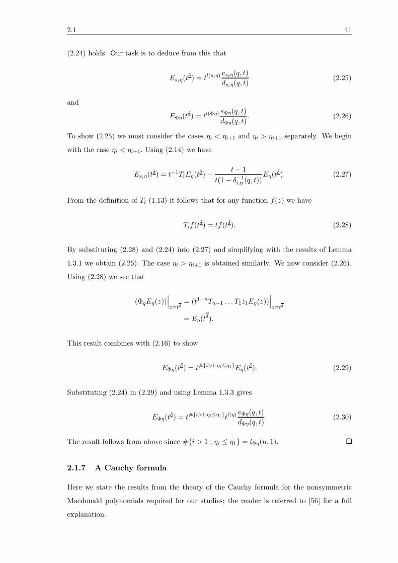
2.1 41
(2.24) holds. Our task is to deduce from this that
Esiη(tδ) = tl(siη)
esiη(q, t)
dsiη(q, t)(2.25)
and
EΦη(tδ) = tl(Φη) eΦη(q, t)
dΦη(q, t). (2.26)
To show (2.25) we must consider the cases ηi < ηi+1 and ηi > ηi+1 separately. We begin
with the case ηi < ηi+1. Using (2.14) we have
Esiη(tδ) = t−1TiEη(t
δ)−t− 1
t(1− δ−1i,η (q, t))
Eη(tδ). (2.27)
From the definition of Ti (1.13) it follows that for any function f(z) we have
Tif(tδ) = tf(tδ). (2.28)
By substituting (2.28) and (2.24) into (2.27) and simplifying with the results of Lemma
1.3.1 we obtain (2.25). The case ηi > ηi+1 is obtained similarly. We now consider (2.26).
Using (2.28) we see that
(ΦqEη(z))∣∣∣z=tδ
= (t1−nTn−1 . . . T1z1Eη(z))∣∣∣z=tδ
= Eη(tδ).
This result combines with (2.16) to show
EΦη(tδ) = t#i>1:ηi≤η1Eη(t
δ). (2.29)
Substituting (2.24) in (2.29) and using Lemma 1.3.3 gives
EΦη(tδ) = t#i>1:ηi≤η1tl(η)
eΦη(q, t)
dΦη(q, t). (2.30)
The result follows from above since #i > 1 : ηi ≤ η1 = lΦη(n, 1).
2.1.7 A Cauchy formula
Here we state the results from the theory of the Cauchy formula for the nonsymmetric
Macdonald polynomials required for our studies; the reader is referred to [56] for a full
explanation.

42 2.2
Lemma 2.1.12. [60] Let
Ω(x, y; q, t) :=∑
η
dηd′ηEη(x; q, t)Eη(y; q
−1, t−1). (2.31)
We have
T(x)i Ω(x, y−1; q, t) = T
(y)i Ω(x, y−1; q, t),
where the superscripts denote which variables the respective operators act upon.
Using Lemma 2.1.12 and (2.14) we are able to deduce an explicit formula for
TiEη(z−1; q−1.t−1).
Proposition 2.1.13. For 1 ≤ i ≤ n− 1 and Eη(z−1) := Eη(z
−1; q−1, t−1) we have
TiEη(z−1) =
t−11−δ−1
i,η (q,t)Eη(z
−1) +dsiηd
′η
d′siηdη
(1−tδi,η(q,t))(1−t−1δi,η(q,t))(1−δi,η(q,t))2
Esiη(z−1), ηi < ηi+1
tEη(z−1), ηi = ηi+1
t−11−δ−1
i,η (q,t)Eη(z
−1) + tdsiηd
′η
d′siηdηEsiη(z
−1), ηi > ηi+1.
(2.32)
Proof. By Lemma 2.1.12
T(x)i
(dηd′ηEη(x)Eη(y
−1) +dsiηd′siη
Esiη(x)Esiη(y−1))
= T(y)i
(dηd′ηEη(x)Eη(y
−1) +dsiηd′siη
Esiη(x)Esiη(y−1)).
Using (2.14) and equating coefficients of like terms gives (2.32) .
2.2 Nonsymmetric Interpolation Macdonald Polynomials
2.2.1 Introduction
The nonsymmetric interpolation Macdonald polynomials E∗η(z) := E∗
η(z; q, t) are the in-
homogeneous analogues of the nonsymmetric Macdonald polynomials Eη(z) and were in-
troduced by Knop and Sahi in [44] and [67], respectively. Although the interpolation
Macdonald polynomials are not homogeneous, like the Macdonald polynomials they per-
mit a number of distinct characterisations which can be taken as their definition. Here we
present the details of such definitions, important to our subsequent workings. The first
definition characterises the polynomials according to their vanishing properties.

2.2 43
2.2.2 The vanishing condition
The interpolation Macdonald polynomials in one variable generalise the monomial zp to
the polynomial
fp(z) := z(z − 1) . . . (z − p+ 1).
This is the unique polynomial, up to normalisation, of degree at most p that vanishes at
z = 0, 1, . . . , p−1 and is non-zero at z = p.We now show how the interpolation Macdonald
polynomials in n variables can also be defined by vanishing conditions.
Lemma 2.2.1. [44] With ηn 6= 0 we have Φ−1η = (ηn/q, η1, . . . , ηn−1).
Proof. Follows from the definition of η, (2.11).
Theorem 2.2.2. [44, 67] Let d ∈ N and S(n, d) be the set of all η where |η| ≤ d. Let
the values of f(η) be prescribed. Then there exists a unique polynomial f(z) of degree at
most d such that f(z) = f(z) for all z ∈ S(n, d).
Proof. Due to the bijection between compositions η and monomials zη the size of S(n, d)
equals the dimension of the space of polynomials of degree at most d. Hence showing f(z)
exists will imply its uniqueness. To show existence, we proceed by induction on n and d.
It is true that every polynomial can be uniquely written as
f(z1, . . . , zn) = g(z1, . . . , zn−1) + (zn − t−n+1)h(zn/q, z1, . . . , zn−1). (2.33)
Let S0 be the set of η ∈ S(n, d) with ηn = 0, or equivalently, η such that ηn = t−n+1.
As z runs through S0, z′ := (z1, . . . , zn−1) will run through S(n − 1, d). By induction,
one can choose g(z) such that f(z) takes the required values at S0. Consider now the
set S1 of remaining points η with ηn 6= 0. By Lemma 2.2.1, as z runs through S1, z′′ :=
(zn/q, z1, . . . , zn−1) will run through S(n, d−1). By appropriately choosing q and t we can
ensure the factor zn − t−n+1 = ηn − t−n+1 is non-zero. By induction, we can find h(z) of
degree at most d − 1 with arbitrary values at S(n, d − 1). Consequently f(z) exists and
the theorem holds.
Theorem 2.2.3. [44, 67] For every composition η there is a unique polynomial E∗η(z)
with triangular structure
E∗η(z) = zη +
∑
λ:|λ|≤|η|,λ6=η
Kηλzλ, Kηλ ∈ Q(q, t) (2.34)

44 2.2
that satisfies (1.56).
With the normalisation specified by (2.34), the polynomial E∗η(z) is referred to as the
nonsymmetric interpolation Macdonald polynomial.
Proof. By Theorem 2.2.2, there is a unique polynomial E∗η(z) satisfying the vanishing
condition with E∗η(η) 6= 0. We have to show that it contains zη with a non-zero coefficient.
Consider (2.33) with f(z) = E∗η(z). If ηn = 0, then g = E∗
η′(z) with η′ := (η1, . . . , ηn−1). By
induction, g(z), and therefore E∗η(z), contain z
η. If ηn 6= 0 then g(z) = 0 and h(z) = E∗η(z).
We conclude again by induction.
2.2.3 The eigenoperators
The second definition of the interpolation polynomials classifies them as the unique simul-
taneous eigenfunctions of the operators Ξi defined by
Ξi := z−1i + z−1
i Hi . . . Hn−1Φ∗qH1 . . . Hi−1. (2.35)
Here
Hi :=(t− 1)zizi − zi+1
+zi − tzi+1
zi − zi+1si (2.36)
= t+zi − tzi+1
zi − zi+1(si − 1) (2.37)
(cf. (1.13)) is the Hecke operator and Φ∗q is the interpolation analogue of Φq (2.15) defined
Φ∗q := (zn − t−n+1)∆, (2.38)
where ∆f(z1, . . . , zn) = f(zn/q, z1, . . . , zn−1). We note that the Hecke operator is another
realisation of the type-A Hecke algebra (1.12).
To show the eigenoperator properties of the interpolation Macdonald polynomials we
must first give explicit formulas to show how the Hecke operator Hi and the raising
operator Φ∗q act on a general function f(z) evaluated at η.
Lemma 2.2.4. [44] Let f(z) be a Laurent polynomial. Then Hif(η) is a linear combina-
tion of f(η) and f(siη) where the coefficients are independent of f(z).
Proof. By (2.36) we have
Hif(η) =(t− 1)ηiηi − ηi+1
f(η) +ηi − tηi+1
ηi − ηi+1
f(siη).

2.2 45
The result follows since either ηi 6= ηi+1 and siη = siη, or, ηi = ηi+1 and ηi−tηi+1 = 0.
Lemma 2.2.5. [44] Let f(z) be a Laurent polynomial. We have
Φ∗qf(Φη) = (qη1 − t−n+1)f(η).
Proof. Follows from the definition of Φ∗q.
After showing that the interpolation Macdonald polynomials are eigenfunctions of Ξi
we use the operators Ξi to determine the relationship between the nonsymmetric Macdon-
ald polynomials and the interpolation Macdonald polynomials.
Theorem 2.2.6. [44] For all i = 1, . . . , n we have
ΞiE∗η(z) = η−1
i E∗η(z). (2.39)
Proof. We begin by rewriting the left hand side of (2.39) as
z−1i (E∗
η(z) +Hi . . . Hn−1Φ∗qH1 . . . Hi−1E
∗η(z)). (2.40)
By Lemmas 2.2.4 and 2.2.5 and the vanishing properties of E∗η(z) (2.40) will vanish at
λ such that |λ| ≤ |η| , λ 6= η. This implies that ΞiE∗η(z) = cE∗
η(z) for some c ∈ Q(q, t).
Evaluation at z = η implies c = η−1i .
Corollary 2.2.7. [44] The operators Ξ1, . . . ,Ξn commute pairwise.
In [44] Knop showed the top homogeneous component of E∗η(z; q, t) to beEη(z; q
−1, t−1).
To define the eigenoperator of Eη(z; q−1, t−1) we require a further realisation of the type-A
Hecke algebra, Hi, given by
H i :=(t− 1)zi+1
zi − zi+1+zi − tzi+1
zi − zi+1si
=Hi + 1− t
The operator H i is seen to be a realisation of the type-A Hecke algebra by observing that
(1.12) is invariant under the mapping hi 7→ hi+1− t. The H i appear in the eigenoperator
of Eη(z; q−1, t−1) according to [44]
ξ−1i := H i . . . Hn−1∆H1 . . . Hi−1.

46 2.2
Theorem 2.2.8. [44] The top homogeneous component of E∗η(z; q, t) is Eη(z; q
−1, t−1).
Proof. Straight forward manipulations show that
Ξn = ξ−1n + z−1
n (1− t−n+1ξ−1n ),
that is Ξn = ξ−1n + degree lowering operators. It follows from this that Ξi = ξ−1
i + degree
lowering operators and therefore E∗η(z; q, t) = Eη(z; q
−1, t−1) + lower order terms.
Theorem 2.2.8 allows us to introduce an isomorphism Ψ mapping each nonsymmetric
Macdonald polynomial to its corresponding interpolation polynomial,
ΨEη(z; q−1, t−1) = E∗
η(z; q, t). (2.41)
This relationship is fundamental to our study of the Pieri-type formulas, allowing us to
use interpolation Macdonald polynomial theory to derive explicit formulas for coefficients
in expansions involving nonsymmetric Macdonald polynomials.
We conclude this section by showing how the eigenoperator Ξi can be used to give
a more precise structure to (2.34). The result is due to Knop [44], however below an
alternative derivation is given.
Lemma 2.2.9. We have
Ξizη = η−1
i zη +∑
λ⊳η
Nηλzλ, Nηλ ∈ Q(q, t), (2.42)
where ⊳ is specified by (1.52)
Proof. The left hand side of (2.42) is written explicitly as
Ξizη = z−1
i zη + z−1i Hi . . . Hn−1(zn − tn+1)∆H1 . . . Hi−1z
η. (2.43)
The composition labelling the first component of (2.43) is λ = (η1, . . . , ηi− 1, . . . , ηn), and
clearly λ ⊳ η. As for the second component of (2.43) we reduce the problem further by
only considering the expansion of
z−1i Hi . . . Hn−1zn∆H1 . . . Hi−1z
η. (2.44)

2.2 47
This is possible since any zλ in the expansion of (2.44) will correspond to a zλ′in the
expansion of z−1i Hi . . . Hn−1t
−n+1∆H1 . . . Hi−1zη and the substitution of zn for t−n+1
forces λ′ ⊳ λ.
With zn∆zη = zΦη and the Hecke operator Hi acting on monomials according to
Hi(zη) =
zsiη, ηi < ηi+1
tzη, ηi = ηi+1
tzsiη + (t− 1)zη , ηi > ηi+1,
(2.45)
it can be seen with some work that the monomials zλ appearing in the the expansion of
(2.44) will be such that
λj ≤ ηj for j 6= i. (2.46)
To show λ ⊳ η we consider the following two cases. Let ηk be the component of η that is
raised by the action of zn∆. If ηk + 1 ≥ maxηi+1, . . . ηn then λi = ηk, λ+ = η+ and by
(2.46) we have λ ⊳ η. Alternatively if ηk + 1 < maxηi+1, . . . ηn some of the monomials
zλ appearing in the the expansion of (2.44) will have λ = σ(η1, . . . , ηk +1, . . . , ηi, . . . , ηj −
1, . . . ηn), for some permutation σ, where ηj > ηk. In this case λ+ 6= η+ and λ+ ≤ η+. It
follows from (2.45) and the action of ∆ that the coefficient of zη is η−1i .
Theorem 2.2.10. [44] The interpolation nonsymmetric Macdonald polynomials are of
the form
E∗η(z) = zη +
∑
λ⊳η
Kηλzλ, Kηλ ∈ Q(q, t). (2.47)
Proof. By the triangularity of Ξi there must be an eigenfunction of the form (2.47) with
eigenvalue η−1i . Thus, it is equal to E∗
η(z).
2.2.4 Recursive generation
Another defining characteristic of the interpolation Macdonald polynomials relates to the
recursive generation (cf (2.14), (2.15)). The interpolation Macdonald polynomials can be
recursively generated by two types of elementary operators, the Hecke operator given by
(2.36) and the raising operator Φ∗q specified by (2.38).
We first consider how the Hecke operator relates E∗η(z)to E
∗siη(z).
Lemma 2.2.11. [44] If ηi = ηi+1 then HiE∗η(z) = tE∗
η(z).

48 2.2
Proof. With E := HiE∗η(z) and λ such that |λ| ≤ |η|, λ 6= η we have E∗
η(λ) = E∗η(siλ) = 0.
By Lemma 2.2.4 E(λ) = 0 and hence E is a multiple of Eη(z). Evaluation at z = η implies
that the factor is t.
Lemma 2.2.12. [67] When ηi 6= ηi+1, we have
(Hi +
1− t
1− δ−1i,η
)E∗
η(z) = kE∗siη(z), k ∈ Q(q, t) (2.48)
where δi,η is given by (1.43).
Proof. Evaluating the right hand side of (2.48) at λ and using Lemma 2.2.4 gives
(Hi +
1− t
1− δ−1i,η
)E∗
η(λ) =(t− 1)λi
λi − λi+1
E∗η(λ) +
λi − tλi+1
λi − λi+1
E∗η(siλ) +
1− t
1− ηi+1/ηiE∗
η(λ).
(2.49)
By the vanishing properties of E∗η(z) (2.49) will vanish for all λ where |λ| ≤ |η| and
λ 6= η, siη. In the case where λ = η the inner term vanishes and the outer terms are equal,
consequently (2.49) vanishes. On the other hand if λ = siη, evaluation of (2.49) gives
E∗siη(siη) =
(siη)i − t(siη)i+1
(siη)i − (siη)i+1E∗
η(η),
since ηi 6= ηi+1 and (siη)i − t(siη)i+1 6= 0 it follows that E∗siη(siη) 6= 0. These vanishing
conditions imply (2.48).
The following results - due to Sahi [67] and Knop [44], respectively, but to be derived
differently below - determine the value of k in Lemma 2.2.12.
Theorem 2.2.13. When ηi < ηi + 1, we have
(Hi +
1− t
1− δ−1i,η
)E∗
η(z) = E∗siη(z). (2.50)
Proof. Due to Lemma 2.2.12 we are only required to show that the coefficient of zsiη in
the left hand side of (2.50) is unity. The triangular structure of E∗η(z) (2.47) implies that
the monomial zsiη does not appear in the expansion of E∗η(z) and the coefficient of zη is
1. Therefore, we only need to consider the action of Hi + (1 − t)/(1 − δ−1i,η ) on z
η. Using
the identityzmi − zmjzi − zj
= zm−1i + zm−2
i zj + . . .+ zm−1j , (2.51)
the coefficient of zsiη is found to be 1, from which the theorem follows.

2.2 49
Theorem 2.2.14. When ηi > ηi+1, we have
(Hi +
1− t
1− δ−1i,η
)E∗
η(z) =(1− tδi,η(q, t))(t− δi,η(q, t))
(1− δi,η(q, t))2E∗
siη(z). (2.52)
Proof. As in the previous theorem we seek the coefficient of zsiη in the left hand side
of (2.52). By viewing η with ηi > ηi+1 as siη′ with η′ such that η′i < η′i+1 we can use
the previous theorem to show that the coefficient of zsiη in E∗η(z) is (1 − t)/(1 − δ−1
i,η ).
Consequently the coefficient of zsiη in the left hand side of (2.52) is found by computing
the action of Hi + (1− t)/(1 − δ−1i,η ) on z
η + (1− t)/(1− δi,η)zsiη. Using straight forward
calculations and the identity (2.51) the desired result is obtained.
We now consider the relationship between E∗η(z) and E
∗Φη(z).
Proposition 2.2.15. [44] We have Φ∗qE
∗η(z) = q−η1E∗
Φη(z).
Proof. By Lemma 2.2.5 we have Φ∗qE
∗η(z)(Φλ) = (qλ1 − t−n+1)E∗
η (z)(λ). The vanishing
properties of E∗η(z) imply Φ∗
qE∗η(z) vanishes for all υ = Φλ such that |υ| ≤ |η| + 1 and
υ 6= Φη. Thus Φ∗qE
∗η(z) = cE∗
Φη(z) for some constant c. Since zΦη = zη21 . . . zηnn−1zη1+1n is
the leading term of E∗Φη(z) and the leading term of Φ∗
qE∗η(z) is
(zn − t−n+1)q−η1zη1n zη21 . . . zηn1 = q−η1zΦη,
we have that c = q−η1 .
With E∗(0,...,0)(z) := 1 the results of this section provide us with a third definition for
the interpolation Madconald polynomials, namely the recursive generation according to
the formulas
HiE∗η(z) =
t−11−δ−1
i,η (q,t)E∗
η(z) + E∗siη(z), ηi < ηi+1
tE∗η(z) , ηi = ηi+1
t−11−δ−1
i,η (q,t)E∗
η(z) +(1−tδi,η(q,t))(t−δi,η (q,t))
(1−δi,η(q,t))2E∗
siη(z), ηi > ηi+1,
(2.53)
Φ∗qE
∗η(z) =q
−η1E∗Φη(z). (2.54)

50 2.2
2.2.5 Rodrigues formula
Since the interpolation Macdonald polynomials have similar recursive generation formulas
to the nonsymmetric Macdonald polynomials it follows naturally that there exists Ro-
drigues formulas that can also be used to compute them. The Rodrigues formulas for
the interpolation polynomials can be found in the literature as they are a limit of the
Rodrigues formulas for the Al-Salam Carlitz polynomials [7]. Here we provide an alterna-
tive derivation of the Rodrigues formulas for the interpolation polynomials using only the
theory contained in this section.
Following the methods in Section 2.1.4 we begin by defining some new operators. We
have the braid exclusion operator
X∗i := ΞiHi −HiΞi,
and the raising-type operator
B∗i := X∗
i . . . X∗n−1Φ
∗q, i = 1, . . . , n − 1
B∗n := Φ∗
q ,
(cf. (2.17) and (2.18)). The final operator is the raising-type operator A∗i , and is defined
to be
A∗i := (B∗
i )i.
Corollary 2.2.16. With κ = η+, |0〉 := 1 and X∗σ as in (1.5) we have
E∗η(z; q, t) = bηX
∗ωη(A∗
1)κ1−κ2(A∗
2)κ2−κ3 . . . (A∗
n)κn |0〉, bη ∈ Q(q, t).
Proof. Since the algebraic relations of Ξi,Hi and Φ∗q mirror those of Yi, Ti and Φq, respec-
tively the proof follows using the same arguments as Theorem 2.1.8.
2.2.6 Evaluation formula
The following proposition uses the discussed properties of the interpolation Macdonald
polynomials to give an evaluation formula for E∗η(η). This evaluation is quite valuable in
the Pieri formula study. An inductive approach is used in a similar way to Proposition
2.1.11.
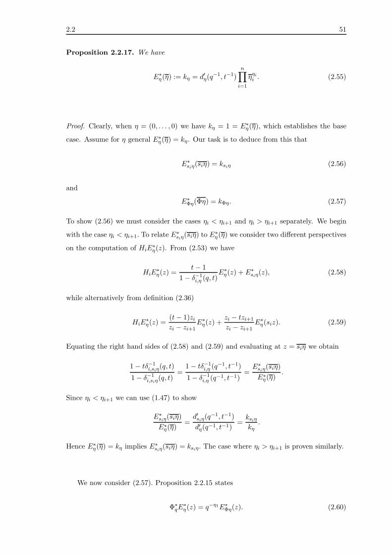
2.2 51
Proposition 2.2.17. We have
E∗η(η) := kη = d′η(q
−1, t−1)
n∏
i=1
ηηii . (2.55)
Proof. Clearly, when η = (0, . . . , 0) we have kη = 1 = E∗η(η), which establishes the base
case. Assume for η general E∗η(η) = kη. Our task is to deduce from this that
E∗siη(siη) = ksiη (2.56)
and
E∗Φη(Φη) = kΦη. (2.57)
To show (2.56) we must consider the cases ηi < ηi+1 and ηi > ηi+1 separately. We begin
with the case ηi < ηi+1. To relate E∗siη(siη) to E
∗η(η) we consider two different perspectives
on the computation of HiE∗η(z). From (2.53) we have
HiE∗η(z) =
t− 1
1− δ−1i,η (q, t)
E∗η(z) + E∗
siη(z), (2.58)
while alternatively from definition (2.36)
HiE∗η(z) =
(t− 1)zizi − zi+1
E∗η(z) +
zi − tzi+1
zi − zi+1E∗
η(siz). (2.59)
Equating the right hand sides of (2.58) and (2.59) and evaluating at z = siη we obtain
1− tδ−1i,siη
(q, t)
1− δ−1i,siη
(q, t)=
1− tδ−1i,η (q
−1, t−1)
1− δ−1i,η (q
−1, t−1)=E∗
siη(siη)
E∗η(η)
.
Since ηi < ηi+1 we can use (1.47) to show
E∗siη(siη)
E∗η(η)
=d′siη(q
−1, t−1)
d′η(q−1, t−1)
=ksiηkη
.
Hence E∗η(η) = kη implies E∗
siη(siη) = ksiη. The case where ηi > ηi+1 is proven similarly.
We now consider (2.57). Proposition 2.2.15 states
Φ∗qE
∗η(z) = q−η1E∗
Φη(z). (2.60)

52 2.2
By evaluating (2.60) at z = Φη, using Lemma 2.2.4 and rearranging we obtain
E∗Φη(Φη)
E∗η(η)
= qη1(qη1 − t−n+1). (2.61)
By using (1.49) and the definition of η we can simplify (2.61) to
E∗Φη(Φη)
E∗η(η)
= q2η1+1t−l′η(1)d′Φη(q
−1, t−1)
d′η(q−1, t−1)
=kΦη
kη. (2.62)
Where the final equality follows from
∏ni=1Φη
(Φη)ii∏n
i=1 ηηii
=Φη
(Φη)nn
ηη11=
(qη1)η1+1
η2η11
= qη1+1t−lη(1).
This completes the proof by induction.
2.2.7 The extra vanishing theorem
It was found by Knop [44] that the interpolation polynomials E∗η(z) vanish on a larger
domain than λ such that |λ| ≤ |η|, λ 6= η. To state this domain we use the partial ordering
′ defined in Section 1.4.2.
In [44] Knop shows that if η 6′ λ then E∗η(λ) = 0 using eigenoperator and the defining
vanishing properties of the interpolation polynomials. Here we prove his result employing
an alternative method that uses the polynomials recursive generation properties as well.
Furthermore it is the main result of this section that E∗η(λ) = 0 if and only if η 6′ λ.
We now work towards showing the main result by first considering λ such that |λ| =
|η| + 1. The results in this section depend heavily on the theory of successors contained
in Section 1.4.2.
Proposition 2.2.18. For λ such that |λ| = |η| + 1 we have E∗η(λ) = 0 if and only if
η 6′ λ.
Proof. Rewriting the eigenoperator Ξi as
ziΞi − 1 = Hi . . . Hn−1Φ∗qH1 . . . Hi−1

2.2 53
and making note of the recursive generation formulas (2.54) and (2.53) shows us that
(ziΞi − 1)E∗η (z) =Hi . . . Hn−1Φ
∗qH1 . . . Hi−1E
∗η(z)
(ziη−1i − 1)E∗
η (z) =∑
ν:ν=cI(η)
CηνE∗ν(z), Cην ∈ Q(q, t), (2.63)
where the summation restriction in (2.63) to ν = cI(η) is a consequence of Proposition
1.4.1. By evaluating (2.63) at λ and using the vanishing conditions of the interpolation
polynomials we see that E∗η(λ) = 0 if and only if λ 6= cI(η), that is, if and only if η 6′ λ.
Proposition 2.2.19. We have E∗η(λ) = 0 if and only if η 6′ λ.
Proof. Here we prove the equivalent statement E∗η(λ) 6= 0 if and only if η ′ λ. We begin
with λ such that |λ| = |η| + 2. By Corollary 1.4.6 we know that λ = cI2cI1(η) for some
sets I1, I2, Ik = kt1, . . . ,kts ⊆ 1, . . . , n with 1 ≤ kt1 < . . . < kts ≤ n.
Taking i = 1t1 in (2.63) gives
(z1t1η−11t1
− 1)E∗η(z) =
∑
ν:ν=cI(η)
CηνE∗ν(z), Cην ∈ Q(q, t).
Proposition 1.4.1 can be used to show E∗cI1 (η)
(z) is in the summation and by Proposition
2.2.18 we know E∗cI1 (η)
(λ) 6= 0. We can be sure that (λ1t1η−11t1
− 1) 6= 0 since even if
λ1t1 = η1t1 we would still have either λ = η/t or λ = η/t2 due to the increased value
of l′η(1t1). These results together show E∗
η(λ) 6= 0 if η ′ λ. For the converse we use an
evaluated form of (2.63) and let i be the position of the leftmost component of η that does
not occur with the same frequency in λ,
(λiη−1i − 1)E∗
η(λ) =∑
ν:ν=cI(η)
CηνE∗ν(λ), Cην ∈ Q(q, t). (2.64)
By the assumption E∗η(λ) 6= 0 and as before (λiη
−1i − 1) 6= 0, consequently there exists a
Eν(λ) on the right hand side of (2.64) that does not vanish and by Proposition 2.2.18 we
have ν ′ λ. Since ν = cI(η) implies η ′ ν we can use Corollary 1.4.4 to show η ′ λ,
which completes the proof for the case |λ| = |η| + 2. Applying this procedure iteratively
shows the result holds for general λ.
2.2.8 Binomial coefficients
In Section 2.2.1, equation (2.2.2), we introduced the one variable interpolation polynomials
fp(z). These polynomials evaluated at l and p such that l > p can be used to define the
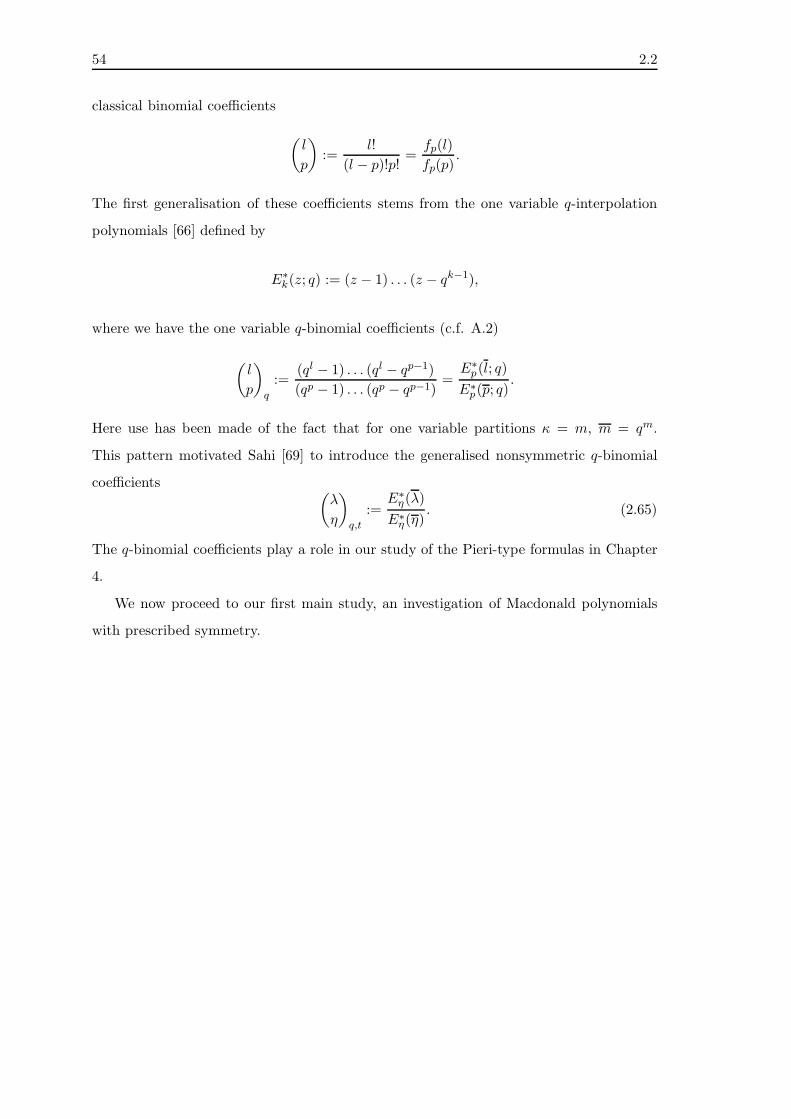
54 2.2
classical binomial coefficients
(l
p
):=
l!
(l − p)!p!=fp(l)
fp(p).
The first generalisation of these coefficients stems from the one variable q-interpolation
polynomials [66] defined by
E∗k(z; q) := (z − 1) . . . (z − qk−1),
where we have the one variable q-binomial coefficients (c.f. A.2)
(l
p
)
q
:=(ql − 1) . . . (ql − qp−1)
(qp − 1) . . . (qp − qp−1)=E∗
p(l; q)
E∗p(p; q)
.
Here use has been made of the fact that for one variable partitions κ = m, m = qm.
This pattern motivated Sahi [69] to introduce the generalised nonsymmetric q-binomial
coefficients (λ
η
)
q,t
:=E∗
η(λ)
E∗η(η)
. (2.65)
The q-binomial coefficients play a role in our study of the Pieri-type formulas in Chapter
4.
We now proceed to our first main study, an investigation of Macdonald polynomials
with prescribed symmetry.

Chapter 3
Macdonald Polynomials with
Prescribed Symmetry
The Macdonald polynomials with prescribed symmetry are obtained from the nonsymmet-
ric Macdonald polynomials via the operations of t-symmetrisation, t-antisymmetrisation
and normalisation. The study of Macdonald polynomials with prescribed symmetry began
in 1999 [2, 56] and was initially motivated by the analogous results in Jack polynomial
theory [4]. Jack polynomials are eigenfunctions of an operator that stems from the type-A
Calogero-Sutherland quantum many body system (see e.g. [23, Chap. 11]). There are
cases where the system is multicomponent, containing both bosons and fermions. In such
cases the system requires eigenfunctions that are symmetric or antisymmetric, with re-
spect to certain sets of variables. This requirement lead naturally to the introduction of
Jack polynomials with prescribed symmetry [4, 42].
We seek a more comprehensive theory of Macdonald polynomials with prescribed sym-
metry, in keeping with the more extensively studied Jack analogues. Our first result is an
expansion formula for the prescribed symmetry Macdonald polynomials in terms of the
nonsymmetric Macdonald polynomials (Proposition 3.2.1). Following this we determine
the normalisation required to obtain the prescribed symmetry Macdonald polynomial from
the symmetrisation of the nonsymmetric polynomial (Proposition 3.2.2). In Section 3.4.1
eigenoperator methods are used to relate the symmetric and antisymmetric Macdonald
polynomials (Proposition 3.3.1), thus providing an alternate proof for a result of Marshall
[57]. We also give an explicit formula for prescribed symmetry polynomials with antisym-
metric components in specific decreasing block form in terms of Vandermonde products
and symmetric Macdonald polynomials (Theorem 3.4.4). Our final investigation is of
the inner product of prescribed symmetry Macdonald polynomials, giving general explicit
55

56 3.2
formulas (Theorem 3.5.2) and then again considering the cases where the antisymmetric
components are in decreasing block form (Theorem 3.5.3). It turns out that these results
have applications in q-constant terms identities, which are discussed in the second half
of Section 3.5. We complete the chapter with a discussion of possible extensions of the
theory.
3.1 A Brief History
Multivariable polynomials with prescribed symmetry have a short history only dating
back to the late 1990’s. There exists prescribed symmetry theory on Jack polynomials,
the generalised Hermite, Laguerre and Jacobi polynomials [4] and Macdonald polynomials
[2]. For each class it is known how to construct the polynomials and also which operator
they are eigenfunctions of. The prescribed symmetry theory of Jack polynomials is the
most well developed and we refer the reader to [25] for many key results. The Macdonald
polynomials with prescribed symmetry were first introduced by Marshall [56] two years
after the introduction of Jack polynomials with prescribed symmetry. Marshall determined
the operator required to transform nonsymmetric Macdonald polynomials to Macdonald
polynomials with prescribed symmetry and the polynomial’s eigenfunction properties.
3.2 Preliminaries
3.2.1 Symmetrisation
We have stated that symmetric Macdonald polynomials Pκ(z) can be obtained from the
nonsymmetric polynomials using U+ (1.14). Similarly, the antisymmetric Macdonald poly-
nomials, denoted Sκ+δ(z) where δ := (n−1, . . . , 1, 0), are obtained from the nonsymmetric
Macdonald polynomials using U− (1.15). In this chapter we generalise these actions by
applying a combination of t-symmetrising and t-antisymmetrising operators to Eη(z) to
generate the Macdonald polynomials with prescribed symmetry.
To do this the notions of symmetric and antisymmetric polynomials from Section 1.2
need to be made more specific by considering the symmetry of particular variables. We
say a polynomial f(z) is symmetric with respect to zi if
sif (z) = f (z)

3.2 57
and antisymmetric with respect to zj if
sjf (z) = −f (z) .
These symmetries naturally generalise to t-symmetries as follows. A polynomial f(z) is
t-symmetric with respect to zi if
Tif (z) = tf (z)
and t-antisymmetric with respect to zj if
Tjf (z) = −f (z) .
3.2.2 Prescribed symmetry operator
We begin our investigation into the Macdonald polynomials with prescribed symmetry
by defining the required symmetrising operator OI,J , first introduced in [56]. In OI,J
the subscripts I, J represent the sets of variables which the operator symmetrises and
antisymmetrises, respectively. Explicitly
Ti[OI,Jf (z)] = tOI,Jf (z) for i ∈ I (3.1)
and
Tj [OI,Jf (z)] = −OI,Jf (z) for j ∈ J. (3.2)
For OI,J to be well defined I and J must be disjoint subsets of 1, . . . , n− 1 satisfying
i− 1, i+ 1 6∈ J for i ∈ I and j − 1, j + 1 6∈ I for j ∈ J.
In many cases we require the set J to be decomposed into disjoint sets of consecutive
integers, to be denoted J1, J2, . . . , Js. For example, with J = 1, 2, 5, 6, 7, J1 = 1, 2 and
J2 = 5, 6, 7. Related to this we also require sets Jj := Jj ∪max (Jj) + 1 and J := ∪Jj.
For the previous example we have J1 = 1, 2, 3, J2 = 5, 6, 7, 8 and J = 1, 2, 3, 5, 6, 7, 8.
Since we are symmetrising with respect to a subset of variables, in contrast to the
construction of U+ and U−, we do not want to sum over all σ ∈ Sn. To define the
restricted set of permutations we use the notation
〈si : i ∈ i1, . . . , ik〉,

58 3.2
which is read to be the set of all permutations that can be constructed using 1, si1 , . . . , sik.
For example 〈si : i ∈ 1, 2〉 = S3 (cf. (1.2)). We introduce WI∪J := 〈sk : k ∈ I ∪ J〉 , a
subset of Sn such that each ω ∈WI∪J ,
ω = ωIωJ , with ωI ∈WI and ωJ ∈WJ , (3.3)
has the property that ω (i) = i if i 6∈ I ∪ J .
The operator OI,J is then specified by
OI,J :=∑
ω∈WI∪J
(−1
t
)l(ωJ )
Tω,
where Tω is as in (1.5).
3.2.3 The polynomial S(I,J)η∗ (z)
To motivate the introduction of the Macdonald polynomials with prescribed symmetry
we first consider the symmetric and antisymmetric Macdonald polynomials, denoted by
Pκ(z) and Sµ+δ(z), respectively, where κ and µ are partitions. To generate Pκ(z) one
would t-symmetrise any Eη(z) for which there exists a permutation σ ∈ Sn such that
ση = κ. Similarly, to generate Sµ+δ(z) one would t-antisymmetrise any Eλ(z) such that
there exists a permutation ρ ∈ Sn where ρλ = µ+ δ. Explicitly
U+Eη(z) = b′ηPκ(z) and U−Eλ(z) = b′′µSµ+δ(z),
for some non-zero b′η, b′′λ ∈ Q (q, t). The importance of µ + δ in the antisymmetric case
is that U−Eµ(z) = 0 if µi = µj for some i 6= j. From the definitions of Pκ(z) and
Sµ+δ(z) it follows that the Macdonald polynomial with prescribed symmetry, denoted
by S(I,J)η∗ (z; q, t) := S
(I,J)η∗ (z), a polynomial t-symmetric with respect to the set I and
t-antisymmetric with respect to the set J , will be labelled by a composition η∗ such that
η∗i ≥ η∗i+1 for all i ∈ I and η∗j > η∗j+1 for all j ∈ J. (3.4)
The polynomial can be generated by applying our prescribed symmetry operator OI,J to
any Eη(z) such that there exists a σ ∈WI∪J with ση = η∗. That is
OI,JEη (z) = a(I,J)η S(I,J)η∗ (z) , (3.5)

3.2 59
for some non-zero a(I,J)η ∈ Q(q, t). This uniquely specifies S
(I,J)η∗ (z) up to normalisation;
for the latter we require that the coefficient of zη∗in the monomial expansion equals unity
as in (2.7).
Our first task is to find the explicit formula for the proportionality a(I,J)η in (3.5). We
do this by first computing the expansion formula of S(I,J)η∗ (z−1; q−1, t−1) := S
(I,J)η∗ (z−1) in
terms of Eη(z−1), a result which is of independent interest.
Proposition 3.2.1. Let ω ∈WI∪J be decomposed as in (3.3). Let ωη∗ = λ and ωIη∗ = λI .
The coefficients in
S(I,J)η∗ (z−1) =
∑
λ∈WI∪J(η∗)
Lη∗λEλ(z−1), Lη∗η∗ = 1, (3.6)
are specified by
Lη∗λ = (−1)l(ωJ ) tl(ωI)d′η∗dλ
d′λIdλI
.
Similarly, the coefficients in
S(I,J)η∗ (z) =
∑
λ∈WI∪J (η∗)
Lη∗λEλ (z) , Lη∗η∗ = 1, (3.7)
are specified by
Lη∗λ =
(−1
t
)l(ωJ ) d′η∗dλ
d′λIdλI
. (3.8)
Proof. We first consider (3.6) and begin by writitng
∑
λ∈WI∪J(η∗)
Lη∗λEλ(z−1)
=∑
λ∈WI∪J(η∗)
λi≤λi+1
χi,i+1
(Lη∗λEλ(z
−1) + Lη∗siλEsiλ(z−1))
where χi,i+1 = 1/2 if λ = siλ and 1 otherwise. For i ∈ I we require
TiS(I,J)η∗ (z−1) = tS
(I,J)η∗ (z−1). (3.9)
If λi = λi+1 (3.9) holds due to the relation in (2.32) . Hence we consider the case where
λi < λi+1. Expanding the left hand side of (3.9) using (2.32) gives simultaneous equations
and solving these show
Lη∗λ
Lη∗siλ
= t(δi,λ − 1)dλd
′siλ
(δi,λ − t)d′λdsiλfor all i ∈ I. (3.10)

60 3.2
Since λi < λi+1 (1.45) can be used to rewrite (3.10) as
Lη∗λ
Lη∗siλ
= td′siλd′λ
. (3.11)
By noting η∗ = ω−1I λI = si1 . . . sil(ω−1
I)λI where each si interchanges increasing components
we can apply (3.11) repeatedly to obtain
Lη∗λI
Lη∗η∗= Lη∗λI
= tl(ωI)d′η∗
d′λI
, (3.12)
where the first equality follows from the normalisation Lη∗η∗ = 1.
To complete the derivation we require a formula for the ratio Lη∗λ/Lη∗λI. Since for all
j ∈ J we have
TjS(I,J)η∗ (z−1) = −S
(I,J)η∗ (z−1),
applying the above methods, with (1.47) in place of (1.45) gives Lη∗λ/Lη∗sjλ = −dλ/dsjλ,
and consequentlyLη∗λ
Lη∗λI
= (−1)l(ωJ) dλdλI
. (3.13)
Combining (3.13) with (3.12) we obtain (3.2.1) .
The derivation of (3.8) is as above, only replacing (2.32) with (2.14).
We now use Proposition 3.2.1 to determine a(I,J)η . To present the result requires some
notation. Write η(ǫI ,ǫJ), where ǫI , ǫJ ∈ +, 0,− , to denote the element of WI∪J (η) with
the properties that η(+,·)(η(·,+)
)has η
(+,·)i ≥ η
(+,·)i+1 for all i ∈ I (η
(·,+)j > η
(·,+)j+1 for all
j ∈ J), η(−,·)(η(·,−)
)has η
(−,·)i ≤ η
(−,·)i+1 for all i ∈ I (η
(·,−)j < η
(·,−)j+1 for all j ∈ J), and η(0,·)
has η(0,·)i = η
(0,·)i+1 for all i ∈ I. For example with λ = ωIωJη
∗ we have ωIη∗ = λ(0,+) and
ωJη∗ = λ(+,0). Also introduce
MI,η :=∑
σ′∈WI
σ′(η)=η(+,0)
tl(σ′).
Proposition 3.2.2. The proportionality constant a(I,J)η in (3.5) is specified by
a(I,J)η = (−1)l(ωJ )MI,η
d′ηd′η(−,+)dη(−,+)
d′η(0,+)dη(0,+)d′
η(−,−)
(3.14)
where ωJ is such that ωJη(+,+) = η(+,0).

3.2 61
Proof. Let G (x, y) be defined by
G (x, y) =∑
η∈WI∪J (η∗)
dηd′ηEη (x)Eη
(y−1). (3.15)
It follows from (2.14) and (2.32) that T(x)i G (x, y) = T
(y)i G (x, y) for i ∈ I ∪ J, and hence
O(x)I,JG (x, y) = O
(y)I,JG (x, y) . (3.16)
By (3.1) and (3.2) we have O(y)I,JEη
(y−1)= b
(I,J)η S
(I,J)η∗
(y−1)for some b
(I,J)η ∈ Q (q, t) .
Hence substituting (3.15) into (3.16) and recalling (3.5) shows
S(I,J)η∗ (x)
∑
η∈WI∪J (η∗)
dηd′ηa(I,J)η Eη
(y−1)= S
(I,J)η∗
(y−1) ∑
η∈WI∪J (η∗)
dηd′ηb(I,J)η Eη (x) .
Using separation of variables it follows that
S(I,J)η∗
(y−1)= aη∗
∑
η∈WI∪J (η∗)
dηd′ηa(I,J)η Eη
(y−1)
(3.17)
for some constant aη∗ ∈ Q(q, t). Equating coefficients for η = ωIωJη∗ in (3.17) and (3.6)
shows
aη∗dηd′ηa(I,J)η = (−1)l(ωJ) tl(ωI)
d′η∗dη
d′η(0,+)dη(0,+)
. (3.18)
The identity (3.18) must hold for all η ∈WI∪J (η∗) , and in particular for η = η(−,−). For
such a composition we can use (2.14) to show
OI,JEη(−,−) (x) = (−1)l(ωJ′ )MI,ηS(I,J)η∗ (x) ,
where ω−1J ′ η(−,−) = η(−,+). Consequently
a(I,J)
η(−,−) = (−1)l(ωJ′)MI,η. (3.19)
Substituting (3.19) into (3.18) with η = η(−,−) implies
aη∗ =tl(ωI)
MI,η
d′η∗d′η(−,−)
d′η(−,+)dη(−,+)
. (3.20)
Substituting (3.20) in (3.18) gives the desired result.

62 3.2
As a corollary of this result we are able to provide an evaluation formula for S(I,∅)η∗ (tδ).
To state the evaluation we require knowledge of how the q-factorial relates to the length
of permutations.
Theorem 3.2.3. [73] For all positive integers n ≥ 2, we have
Ln(q) :=∑
σ∈Sn
ql(σ) = [n]q! (3.21)
where [n]q! denotes the q-factorial (A.1).
Proof. To prove (3.21) we go one further and show that each of the n! terms in the
expansion of Ln(q) corresponds to exactly one permutation in Sn, that is the ith term
corresponding to the permutation σi will be of the form qK1(σi) . . . qKn(σi), where Kj is
given by (1.1). Starting with n = 2 we prove (3.21) inductively. For n = 2 there are 2
permutations, one of length zero and one of length one and hence L2(q) = 1+q as required.
We now assume that the statement is true for n− 1. Let ω = (ω(1), . . . , ω(n− 1)) ∈ Sn−1.
By inserting n somewhere in ω we form a new permutation ω′ ∈ Sn. If n is inserted in the
kth position then for j = k, . . . , n− 1, Kj+1(ω′) = Kj(ω) + 1, hence increasing the length
of the permutation by n− k. Therefore Ln(q) = Ln−1(q)(1 + q+ . . .+ qn−1), which proves
(3.21).
We now present the corollary.
Corollary 3.2.4. We have the evaluation formula
S(I,∅)η∗ (tδ) =
nI
a(I,∅)η∗
Eη∗(tδ) =
nIMI,η∗
tl(η)eη∗
dη∗(−,0)
, (3.22)
where nI := Σσ∈WItl(σ) = Πs[|Is|]t!.
Proof. Using (2.28) the first equality of (3.22) can be derived immediately from (3.5) .
With J = ∅ and η = η∗ Proposition 3.2.2 gives
a(I,∅)η∗ =MI,η∗
dη∗(−,0)
dη∗.
Substituting this and (2.24) intonI
a(I,∅)η∗
Eη∗(tδ)
gives the final equality.

3.3 63
We now move on to our first related result, deducing the form of Macdonald polyno-
mials with prescribed symmetry in specific cases.
3.3 Antisymmetric Macdonald Polynomials
In this section we show how one can express an antisymmetric Macdonald polynomial in
terms of a symmetric Macdonald polynomial and the t-Vandermonde product. This result
is originally due to Marshall [57] and was proven using the polynomials orthogonality
properties and Kadell’s Lemma [40]. Kadell’s Lemma states that for any antisymmetric
function h(z)
CT(∏
i<j
(zi − azj)h(z))=
[n]a!
n!CT(∏
i<j
(zi − zj)h(z)). (3.23)
We first present Marshall’s derivation and then proceed, in the second proof, to use an
eigenoperator method to reclaim the result. It appears that the eigenoperator method
can be adapted to a more general form of prescribed symmetry polynomial; we give the
details of this in the following section.
Proposition 3.3.1. [57] We have
Sκ+δ(z; q, t) = ∆t (z)Pκ (z; q, qt) . (3.24)
Proof 1. To employ Kadell’s Lemma (3.23) we begin by writing the inner product
〈∆t(z)Pκ(z; q, qt),∆t(z)Pµ(z; q, qt)〉q,t as
〈∆t(z)Pκ(z; q, qt),∆t(z)Pµ(z; q, qt)〉q,t = CT(∏
i<j
(zi − t−1zj)h(z)), (3.25)
where
h(z) =∏
i<j
(z−1i − tz−1
j )(ziz
−1j ; q)∞(qzjz
−1i ; q)∞
(tziz−1j ; q)∞(qtzjz
−1i ; q)∞
Pκ(z; q, qt)Pµ(z−1; q−1, (qt)−1)
=∏
i<j
(z−1i − z−1
j )(qziz
−1j ; q)∞(qzjz
−1i ; q)∞
(qtziz−1j ; q)∞(qtzjz
−1i ; q)∞
Pκ(z; q, qt)Pµ(z−1; q−1, (qt)−1)

64 3.3
and is an antisymmetric polynomial. Note that the second equality in the above equation
is due to the simplification
(z−1i − tz−1
j )(1− ziz
−1j )
(1− ziz−1j )
= z−1i − z−1
j .
Applying Kadell’s lemma twice to the right hand side (3.25) we obtain
〈∆t(z)Pκ(z; q, qt),∆t(z)Pµ(z; q, qt)〉q,t =[n]t−1!
[n]qt!
(∏
i<j
(zi − qtzj)h(z))
=[n]t−1!
[n]qt!〈Pκ(z; q, qt), Pµ(z; q, qt)〉q,qt
=[n]t−1!
[n]qt!〈Pκ(z; q, qt), Pκ(z; q, qt)〉q,qtδκµ, (3.26)
here, the second equality is a consequence of
(zi − qtzj)(z−1i − tz−1
j )
(1− tziz−1j )(1− qtziz
−1j )
= 1.
It follows from (3.26) that the polynomials ∆t(z)Pκ(z; q, qt) form an orthogonal set with
respect to 〈·, ·〉q,t. Since the polynomials are also of the form
Sκ+δ(z; q, t) = m′κ+δ(z) +
∑
µ<κ+δ
Kκµm′µ(z), Kκµ ∈ Q(q, t),
where m′κ+δ := U−(zκ+δ), we must have (3.24).
Proof 2. Since the unique symmetric eigenfunction of D1n (q, qt) (1.20) with leading term
mκ(z) (1.8) is Pκ (z; q, qt), we can show (3.24) holds by proving the more general statement
D1n (q, t)∆t (z) f (z) = ∆t (z)D
1n (q, qt) f (z) , (3.27)
where f(z) is any symmetric function. We begin by rewriting D1n(q, t) as [43]
D1n (q, t) := tn−1
n∑
i=1
Yi
and deriving a more explicit form for the left hand side of (3.27). Since ∆t (z) f (z) is
t-antisymmetric the left hand side can be rewritten as
(T1 . . . Tn−1ω − tT2 . . . Tn−1ω + . . .+ (−t)n−1 ω
)∆t (z) f (z)

3.3 65
which, by the definition of ω is equal to
(T1 . . . Tn−1 − tT2 . . . Tn−1 + . . .+ (−t)n−1
)∆t (qzn, z1, . . . , zn−1) f (qzn, z1, . . . , zn−1) .
For simplicity we let Θm := Tm . . . Tn−1, gk(z) := ∆t (qzk, z1, . . . , zn) f (qzk, z1, . . . , zn) and
Ti =(1− t) zi+1
zi − zi+1+tzi − zi+1
zi − zi+1si. (3.28)
We begin by deducing the coefficient, c[k,m] say, of each gk(z) after being operated on by
Θm. Note that by the definition of Θm we have c[k,m] = 0 if m > k. The structure of Ti
in (3.28) indicates that there will be 2n−m terms in the expansion of Θmgn(z). We begin
by focusing on the coefficient of c[k, k]. To obtain gk(z) from gn(z) we must take the term
corresponding to the action oftzi − zi+1
zi − zi+1si
for each i = n− 1, . . . , k + 1, therefore
c[k, k] =
n∏
i=k+1
tzk − zizk − zi
.
It can be shown by (backward) induction on m that for m < k
c[k,m] = (−1)k−m (t− 1) zkzm − zk
k−1∏
i=m+1
tzi − zkzi − zk
n∏
i=k+1
tzk − zizk − zi
.
We note that an important part of the inductive proof is to keep ∆t(z)f(z) expressible in
terms of gk(z). This is done by observing that sif (z) = f (z) and
si∆t (z) =tzi+1 − zitzi − zi+1
∆t (z) .
To derive the coefficient of gk(z) in the overall operator we must evaluate
k∑
m=1
(−t)m−1 c [k,m].
To do this we prove
k∑
m=j
(−t)m−1 c[k,m] = (−t)j−1k−1∏
i=j
zk − tzizi − zk
n∏
i=k+1
tzk − zizk − zi

66 3.3
inductively with a base case of j = k−1. It follows that the coefficient of f (qzk, z1, . . . , zn)
in D1n (q, t)∆t (z) f (z) is
k−1∏
i=1
zk − tzizi − zk
n∏
i=k+1
tzk − zizk − zi
∆t (qzk, z1, . . . , zn) . (3.29)
By noting
∆t (qzk, z1, . . . , zn) =
k−1∏
i=1
qzk − t−1zizi − t−1zk
n∏
i=k+1
qzk − t−1zizk − t−1zi
∆t (z)
we simpify (3.29) to
∆t (z)
n∏
i=1i 6=k
qtzk − zizk − zi
,
and hence
D1n (q, t)∆t (z) f (z) = ∆t (z)
n∑
k=1
n∏
i=1i 6=k
qtzk − zizk − zi
f (qzk, z1, . . . , zn) .
We now simplify the right hand side of (3.27). We have
D1n (q, qt) f (z) = (qt)n−1
n∑
i=1
Y(q,qt)i f (z)
= (qt)n−1((qt)1−n T
(q,qt)1 . . . T
(q,qt)n−1 ω + . . .+ ωT
−1(q,qt)1 . . . T
−1(q,qt)n−1
)f (z)
(3.30)
where Y(q,qt)i , T
(q,qt)i , T
−1(q,qt)i are the operators Yi, Ti, T
−1i with t replaced by qt. Since
f (z) is symmetric we have T−1(q,qt)i f (z) = (qt)−1 f (z) . Using this and the action of ω
(3.30) simplifies to
(T(q,qt)1 . . . T
(q,qt)n−1 + . . .+ T
(q,qt)n−1 + 1)f (qzn, z1, . . . , zn−1) .
We define Θ(q,qt)m := T
(q,qt)m . . . T
(q,qt)n−1 and denote the coefficient of each f (qzk, z1, . . . , zn)
by cq[k,m] for each m ≤ k. Similarly to before
cq[k, k] =n∏
i=k+1
qtzk − zizk − zi

3.4 67
and, by induction,
cq[k,m] = (−1)k−m (qt− 1) zkzm − zk
k−1∏
i=m+1
qtzk − zizi − zk
n∏
i=k+1
qtzk − zizk − zi
.
For use in (3.30) we require∑k
m=1 cq[k,m]. This is found by induction on
k∑
m=j
cq[k,m] =
n∏
i=ji 6=k
qtzk − zizk − zi
.
Therefore
∆t (z)D1n (q, qt) f (z) = ∆t (z)
n∑
k=1
n∏
i=1i 6=k
qtzk − zizk − zi
f (qzk, z1, . . . , zn) ,
which shows (3.27), and consequently (3.24), to be true.
3.4 Prescribed Symmetry Macdonald Polynomials
with Staircase Components
In this section we consider prescribed symmetry Macdonald polynomials labelled by a
composition comprising of a partition κ and p blocks of staircase partitions, denoted δNp
below. These polynomials are symmetric with respect to variables corresponding to κ and
antisymmetric for those corresponding to the staircase components.
In the literature such polynomials appear in two different forms. One with the sym-
metric variables preceding the antisymmetric where η∗, I and J are given explicitly by
η∗ = η(n0;Np) := (κ, δNp) = (κ1, . . . , κn0 , δn1 , . . . , δnp) (3.31)
= (κ1, . . . , κn0 , n1 − 1, n1 − 2, . . . , 1, 0, . . . , np − 1, . . . , 1, 0),
J = Jn0,Np :=
p⋃
α=1
( α∑
k=1
nk−1
)+ 1, . . . ,
( α+1∑
j=1
nk−1
)− 1
(3.32)
and
I = In0,Np := 1, . . . , n0 − 1,

68 3.4
and the other having the opposite ordering with the antisymmetric variables first, for
which we have
η∗ = η(Np;n0) := (δNp , κ) = (δn1 , . . . , δnp , κ1, . . . , κn0) (3.33)
= (n1 − 1, n1 − 2, . . . , 1, 0, . . . , np − 1, . . . , 1, 0, κ1, . . . , κn0),
J := JNp,n0 =
p⋃
α=1
( α−1∑
k=1
nk−1
)+ 1, . . . ,
( α∑
k=1
nk−1
)− 1
and
I = INp,n0 := n− n0 + 1, . . . , n,
where in each case
Np := n1, . . . , np. (3.34)
For example with κ = (4, 4, 2) and Np = 4, 2 we have η(n0;Np) = (4, 4, 2, 3, 2, 1, 0, 1, 0),
In0,Np = 1, 2 and Jn0,Np = 4, 5, 6, 8 and; η(Np;n0) = (3, 2, 1, 0, 1, 0, 4, 4, 2), INp,n0 =
7, 8 and JNp,n0 = 1, 2, 3, 5.
Before stating our major goal for the section we introduce the final ingredients; the
generalised Vandermonde product
∆J (z) :=
p∏
α=1
∏
min(Jα)≤i
<j≤max(Jα)
(zi − zj) ,
(cf. (1.11)), and the generalised t-Vandermonde product ∆Jt (z)
∆Jt (z) :=
p∏
α=1
∏
min(Jα)≤i
<j≤max(Jα)
(zi − t−1zj
),
(cf. (1.17)).
In this section we aim to express S(I,J)η∗ (z; q, t), where η∗, I and J are specified by
either of the above forms, in terms of the generalised Vandermonde product ∆Jt (z) and a
symmetric Macdonald polynomial. Such an expression was motivated by results in both
[4] and [2] and is a generalisation of (1.16).
In [4] Baker and Forrester show that with κ1 < minn1, . . . , np the prescribed sym-
metry Jack polynomial, denoted S(I,J)η∗ (z;α), can be expressed
S(In0,Np ,Jn0,Np)η(n0;Np)
(z;α) := S(I,J)η(n0;Np)
(z;α) = ∆Jn0,Np(z)Pκ(z1, . . . , zn0 ;α+ p). (3.35)

3.4 69
In (3.35) Pκ(z;α) is the symmetric Jack polynomial (refer Appendix B). We note that in
[4] the composition labelling the prescribed symmetry polynomial in (3.35) is incorrectly
documented as
(κ1, . . . , κn0 , n1 − 1, . . . , 2, 1, . . . , np − 1, . . . , 2, 1).
A prescribed symmetry polynomial labelled by such a composition does not satisfy (3.35)
and a close inspection of their proof indicates the composition is required to be of the form
specified by (3.31).
The structure of the prescribed symmetry Jack polynomial S(I,J)η(n0;Np)
(z;α) was obtained
using properties of the eigenoperator in the Jack theory. Due to the different structure of
the Macdonald eigenoperator the methods used in the Jack case can not be generalized.
However, within [4] a brief note is made on how one may show that
Sκ+δ(z;α) = ∆(z)Pκ(z;α/(1 + α)),
(cf. (3.24)), where Sκ+δ(z;α) is the antisymmetric Jack polynomial, using the fact that
H(C,Ex)α ∆(z)f(z) = ∆(z)H
(C,Ex)(α/(1+α))f(z),
(cf. (3.27)). We refer the reader to [4] for the definition of the Jack polynomial eigenop-
erator H(C,Ex)α and further details of the suggested method.
Low order cases indicate that this method can be generalised to prove (3.35). Here
we explain how the eigenoperator proof of Proposition 3.3.1 could be suitably generalised
to prove the Macdonald case of (3.35). Following this we consider the other form of the
special prescribed symmetry polynomials where the antisymmetric components precede
the symmetric. Our motivation is the formula for Macdonald polynomials in the case
p = 1 from [2] that states if κ1 < n1 then
S(I,J)η(n1;n0)
(z; q, t) = ∆Jn1,n0
t (z)Pκ(zn1+1, . . . , zn; qt, t). (3.36)
We generalise the methods used in [2] to show how this result can be extended beyond
the case p = 1.
3.4.1 Special form with η∗ = η(n0;Np)
Computational evidence suggests the following conjecture.

70 3.4
Conjecture 3.4.1. With κ1 < minn1, . . . , np, (I, J) = (In0,Np , Jn0,Np) and η∗ =
η(n0;Np) we have
S(I,J)η∗ (z; q, t) = ∆J
t (z)Pκ(z1, . . . , zn0 ; qtp, t). (3.37)
The proof is yet to be found. It appears to be related to the following conjecture.
Conjecture 3.4.2. Let f (z1, .., zn0) be a symmetric function with leading term mκ(z) and
κ1 < min (n1, . . . , np). We have
D1n (q, t)∆
Jn0,Np
t (z) f (z1, . . . , zn0) = ∆Jn0,Np
t (z)D1n (qt
p, t) f (z1, . . . , zn0) . (3.38)
We believe it to be possible to prove (3.37) by first proving (3.38). At this stage
however it is not clear how one would keep track of the blocks of variables within the anti-
symmetrising set, making the strategy used in the proof of Proposition 3.3.1 problematic
to generalise.
3.4.2 Special form with η∗ = η(Np;n0)
In this section we generalise (3.36) to η∗ specified by (3.33) and show that the condition
κ1 < n1 can be weakened in general to κ1 ≤ minn1, . . . , np. We begin with the specific
case where κ = (0, . . . , 0) and then consider the more general setting.
Theorem 3.4.3. With η∗ = (δNp , 0n0) and (I, J) = (∅, JNp ,n0) we have
S(I,J)η∗ (z; q, t) = ∆J
t (z) .
Proof. The result follows from S(I,J)η∗ (z; q, t) having leading term z(δNp ,0
n0 ) and the require-
ment that S(I,J)η∗ (z; q, t) be t-antisymmetric with respect to J .
To prove the general result we follow the methods of [2, Sect. 3] and hence require
explicit formulas for the action of T−1i on the monomial zai z
bi+1. After this has been
presented we proceed with the theorem.
We have [2]
T−1i zai z
bi+1 =
(t−1 − 1)zai zbi+1 + (t−1 − 1)za−1
i zb+1i+1
+ . . .+ (t−1 − 1)zb+1i za−1
i+1 + t−1zbi zai+1, a > b
t−1zai zai+1, a = b
(1− t−1)za+1i zb−1
i+1 + . . .+ (1− t−1)zb−1i za+1
i+1
+zbi zai+1, a < b.
(3.39)

3.4 71
Theorem 3.4.4. With κ1 ≤ min(n1, . . . , np), (I, J) = (INp,n0 , JNp,n0) and η∗ = η(Np;n0)
we have
S(I,J)η∗ (z; q, t) = ∆J
t (z)Pκ(zn−n0+1, . . . , zn; qtp, t). (3.40)
Proof. Using (3.5) we construct S(I,J)η∗ (z; q, t) with η∗ = η(Np;n0) by
1
a(I,J)η
OI,JEη(z; q, t),
where η = (δRn1, . . . , δRnp
, κR). Such a polynomial is an eigenfunction of the operators
H1 =
n1∑
i=1
Yi, . . . ,Hp =
n−n0∑
i=n1+...+np−1+1
Yi, H0 =
n∑
i=n−n0+1
Yi,
where each Yi acts on all variables z1, . . . , zn. By the definition of the partial order ≺
given in (1.39), the Macdonald polynomial E(δRn1,...,δRnp
,κR)(z; q, t) is of the form
E(δRn1,...,δRnp
,κR)(z; q, t) = z(δRn1
,...,δRnp,κR) +
∑
(δRn1,...,δRnp ,η)≺(δRn1
,...,δRnp ,κR)
K(δRn1,...,δRnp
,η)z(δRn1
,...,δRnp,η)
+∑
γ≺(δRn1,...,δRnp
,η)
Kγzγ (3.41)
for coefficients Kη ∈ Q(q, t), where any γ ≺ (δRn1, . . . , δRnp
, η) contains a pair i, j ∈
Jnk, for some k = 1, . . . , p, such that γi = γj . Consequently when we apply OI,J to
E(δRn1,...,δRnp ,κ
R)(z; q, t) the terms in the latter sum of (3.41) vanish, that is
OI,JE(δRn1,...,δRnp
,κR)(z; q, t) =OI(OJ z(δRn1
,...,δRnp,0n0 ))
×(z(0,...,0,κ
R) +∑
η≺κR
K(δRn1,...,δRnp
,η)z(0,...,0,η)
)
=∆Jt (z)g(zn−n0+1, . . . , zn), cδNp
∈ Q(q, t)
where g is a symmetric polynomial with leading term mκ(zn−n0+1, . . . , zn). To complete
the proof we must show that g(zn−n0+1, . . . , zn) is an eigenfunction of
H′0 =
n∑
i=n−n0+1
Y(qtp,t)i ,
where each Yi acts only on the variables zn−n0+1, . . . , zn. This statement is equivalent to
H0∆Jt (z)g(zn−n0+1, . . . , zn) ∝ ∆J
t (z)H′0g(zn−n0+1, . . . , zn)

72 3.4
which is further simplified by
Y(q,t)i ∆J
t (z)g(zn−n0+1, . . . , zn) ∝ ∆Jt (z)Y
(qtp,t)i g(zn−n0+1, . . . , zn),
where i = n − n0 + 1, . . . , n. Since T−1i does not depend on q and g is symmetric with
respect to the variables zn−n0+1, . . . , zn we are only required to show
ωT−11 . . . T−1
n−n0∆J
t (z)g(zn−n0+1, . . . , zn) ∝ ∆Jt (z)ω
n0qtpg(zn−n0+1, . . . , zn), (3.42)
where ωn0qtp := sn−1 . . . sn−n0+1τ
qtp
n−n0+1, that is ω restricted to act on the variables
zn−n0+1, . . . , zn,
with q replaced by qtp. Since for 1 ≤ i ≤ n− n0 − 1,
T−11 . . . T−1
n−n0Ti = Ti+1T
−11 . . . T−1
n−n0
it follows that
T−11 . . . T−1
n−n0OJ = OJ ′T−1
1 . . . T−1n−n0
,
where J ′ = 2, . . . , n1 ∪pi=2 ni−1 + 2, . . . , ni, and so
T−11 . . . T−1
n−n0∆J
t (z)zκ1n−n0+1 = T−1
1 . . . T−1n−n0
z(δn1 ,...,δnp)zκ1n−n0+1 (3.43)
= OJ ′T−11 . . . T−1
n−n0z(δn1 ,...,δnp)zκ1
n−n0+1. (3.44)
Due to the action of T−1i on monomials zai z
bi+1 specified by (3.39) we have
T−11 . . . T−1
n−n0z(δn1 ,...,δnp)zκ1
n−n0+1 = t−(n−n0+1)+pκ1(z2 . . . zn−n0zn−n0+1)(δn1 ,...,δnp )zκ1
1 + . . . .
(3.45)
Also by the action of T−1i we observe that the additional terms in (3.45) will have terms
containing (z2 . . . zn−n0zn−n0+1)γ where γi = γj for some i, j ∈ Jnk
for some i 6= j and
k = 1, . . . , p. Since such terms will vanish under the action of OJ ′ we can rewrite (3.44) as
OJ ′T−11 . . . T−1
n−n0z(δn1 ,...,δnp)zκ1
n−n0+1 = t−(n−n0+1)∆J ′(z2, . . . , zn−n0 , zn−n0+1)(t
pz1)κ1 .
(3.46)
Since g is a symmetric function it follows from (3.46) and (3.43) that (3.42), and conse-
quently (3.40) holds.

3.5 73
A major result in the theory of Jack polynomials with prescribed symmetry is the
evaluation U(I,J)η∗ (1n;α) [18], where U
(I,J)η∗ (z;α) is defined by
U(I,J)η∗ (z;α) :=
S(I,J)η∗ (z;α)
∆J (z).
The method contained in [18] does not naturally extend to Macdonald theory and the
explicit evaluation of U(I,J)η∗ (tδ; q, t), where
U(I,J)η∗ (z; q, t) :=
S(I,J)η∗ (z; q, t)
∆Jt (z)
remains an open problem. However, for the cases where the prescribed symmetry Mac-
donald polynomials are of the form specified by (3.40) use of the evaluation formula for
the symmetric Macdonald polynomials [54]
Pκ(tδ; q, t) = tl(κ)
∏
s∈diag(κ)
1− qa′η(s)tn−l′η(s)
1− qaη(s)tlη(s)+1(3.47)
gives the following as a corollary to Theorem 3.4.4
U(I,J)η(Np;n0)
(tδ; q, t) = tl(κ)∏
s∈diag(η(Np ,n0))
1− (qtp)a′η(s)tn−l′η(s)
1− (qtp)aη(s)tlη(s)+1. (3.48)
bla
3.5 The Inner Product of Prescribed Symmetry Polynomi-
als and Constant Term Identities
3.5.1 The inner product of prescribed symmetry polynomials
We begin this section by finding the explicit formulas for the inner product of the pre-
scribed symmetry polynomials S(I,J)η∗ (z) := S
(I,J)η∗ (z; q, t)
〈S(I,J)η∗ (z) , S
(I,J)η∗ (z)〉q,t, (3.49)
in terms of the inner product of nonsymmetric Macdonald polynomials. We then proceed
to show how these formulas can be used to prove specialisations of certain constant term
conjectures. We first consider the inner product of OI,JEη(z).

74 3.5
Lemma 3.5.1. Let Ii and Jj denote the decomposition of I and J as a union of sets of
consecutive integers, then with KI,J(t) := Πsi=1[|Jj |]t!Π
ri=1[|Ii|]t−1 ! we have
〈OI,JEη (z) , OI,JEη (z)〉q,t = KI,J(t) 〈OI,JEη (z) , Eη (z)〉q,t . (3.50)
Proof. We begin by rewriting the left hand side of (3.50) as
⟨OI,JEη (z) ,
∑
ω∈WI∪J
(−t)−l(ωJ )TωEη (z)⟩q,t
=∑
ω∈WI∪J
⟨OI,JEη (z) , (−t)
−l(ωJ )TωEη (z)⟩q,t. (3.51)
Since T−1i is the adjoint operator of Ti (1.28), it follows that (3.51) is equal to
∑
ω∈WI∪J
⟨T−1ω OI,JEη (z) , (−t)
−l(ωJ )Eη (z)⟩q,t. (3.52)
Using (3.1) and (3.2) we rewrite (3.52) as
∑
ω∈WI∪J
⟨(−1)l(ωJ ) t−l(ωI)OI,JEη (z) , (−t)
−l(ωJ )Eη (z)⟩q,t.
By definition of the inner product⟨·, t−1
⟩q,t
= 〈t, ·〉q,t and therefore we have
∑
ω∈WI∪J
⟨tl(ωJ )t−l(ωI)OI,JEη (z) , Eη (z)
⟩q,t
=∑
ω∈WI∪J
tl(ωJ)
tl(ωI)〈OI,JEη (z) , Eη (z)〉q,t .
The final result is obtained by employing (3.21).
We can now show how 〈S(I,J)η∗ (z) , S
(I,J)η∗ (z)〉q,t relates to 〈Eη (z) , Eη (z)〉q,t.
Theorem 3.5.2. We have
⟨S(I,J)η∗ (z) , S
(I,J)η∗ (z)
⟩q,t
= KI,J (t)Lη∗η
aη (q−1, t−1)〈Eη (z) , Eη (z)〉q,t , (3.53)
where Lη∗η and aη(q−1, t−1
)are given by (3.8) and (3.14) respectively.
Proof. Using (3.5) we are able to rewrite (3.49) as
⟨a(I,J)η (q, t)−1OI,JEη (z) , a
(I,J)η (q, t)−1OI,JEη (z)
⟩q,t

3.5 75
by the definition of the inner product and Lemma 3.5.1 we write this as
KI,J (t)
a(I,J)η (q, t) a
(I,J)η (q−1, t−1)
〈OI,JEη (z) , Eη (z)〉q,t . (3.54)
Again using (3.5) we rewrite (3.54) as
KI,J (t)
a(I,J)η (q−1, t−1)
⟨S(I,J)η∗ (z) , Eη (z)
⟩q,t.
By (3.7) and the orthogonality of the Macdonald polynomials we get the desired result.
3.5.2 Special cases of the prescribed symmetry inner product
Following the theory of Jack polynomials [2] we were lead to finding explicit formulas for
(3.49) in the special case where
η∗ = η∗(0n0 ;n1):= (0n0 , δn1) = (0, . . . , 0, n1 − 1, . . . , 1, 0),
I = ∅ and J = Jn0,n1 (cf. (3.31)). Upon further inspection of this formula it was observed
that in the limit t → qk the result could be used to provide an alternative derivation of
a specialisation of a constant term conjecture from [3]. Whilst working with the constant
term identities it became apparent that a further conjecture in [3] was related to the more
general inner product formula where
η∗ = η∗(0n0 ;Np):= (0n0 , δNp) = (0, . . . , 0, n1−1, . . . , 1, 0, n2−1, . . . , 1, 0, . . . , np−1, . . . , 1, 0),
(3.55)
I = ∅ and J = Jn0,Np . Note that these compositions and sets are like those in Section
3.4.1 where the symmetric components precede the antisymmetric components.
Using the theory developed in the previous section we give an explicit formula for
⟨S(I,J)η∗(0n0 ;Np)
(z) , S(I,J)η∗(0n0 ;Np)
(z)⟩q,qk
,
deriving the more specific formula with η∗ = η∗(0n0 ;n1)as a corollary.
Theorem 3.5.3. With η∗ = η∗(0n0 ;Np)as defined by (3.55), I = ∅ and J = Jn0,Np we have
⟨S(I,J)η∗ (z), S
(I,J)η∗ (z)
⟩q,qk
=
p∏
i=1
[ni]qk !q−kΣp
i=1
ni(ni−1)2
[kn+max (NP )]q! (1− q)max(NP )
[k]q!nΠmax(Np)j=1
(1− qjqk(n−m(j))
) .
(3.56)

76 3.5
In (3.56) m(j) :=∑p
k=ij(n+k − j), where ij := #n+k ∈ N+
p : n+k < j + 1, with N+p :=
n+1 , . . . , n+p = σ (Np) and n
+1 ≥ . . . ≥ n+p .
Proof. Using (3.53) we see that the task is to simplify
K∅,J(qk)
Lη∗η
aη (q−1, q−k)〈Eη (z) , Eη (z)〉q,qk .
For simplicity we take η = η∗, and hence cη∗η∗ = 1. Since I = ∅ and ω such that ωη∗ = η
is ω = 1 we have
aη∗(q−1, q−k) =
d′η∗(q−1, q−k
)
d′η∗(−,−) (q
−1, q−k).
The p disjoint sets in J indicate that
KI,J(qk) =
p∏
i=1
[ni]qk !
and lastly, by (2.22) and (2.23), we have
⟨Eη∗(z; q, q
k), Eη∗(z; q, qk)⟩q,qk
=d′η∗(q, qk
)eη∗(q, qk
)
dη∗ (q, qk) e′η∗ (q, qk)
[nk]q!
[k]q!n.
Putting this all together allows us to rewrite (3.56) as
p∏
i=1
[ni]qk !d′η∗(−,−)
(q−1, q−k
)d′η∗(q, qk
)eη∗(q, qk
)
d′η∗ (q−1, q−k) dη∗ (q, qk) e
′η∗ (q, q
k)
[nk]q!
[k]q!n.
We begin by simplifyingd′η∗(−,−)
(q−1, q−k
)d′η∗(q, qk
)
d′η∗ (q−1, q−k) dη∗ (q, qk)
. (3.57)
In comparison with diag(η∗), diag(η∗(−,−)) has one additional empty box above each row.
Hence the leg length of each s ∈diag(η∗(−,−)) is one greater than its corresponding box in
diag(η∗) . It follows from this and the definition of dη and d′η that d′η∗(−,−) = dη∗ . Using
this and the identity (1.51) we can write (3.57) as
dη∗(q−1, q−k
)d′η∗(q, qk
)
d′η∗ (q−1, q−k) dη∗ (q, qk)
= qkΣpi=1
ni(ni−1)
2 .
We now consider the simplification of the ratio of eη and e′η. Explicitly we have
eη∗(q, qk
)
e′η∗ (q, qk)
=
∏
s
(1− q
a′η∗
(s)+1qk(n−l′
η∗(s)))
∏
r
(1− q
a′η∗
(r)+1qk(n−1−l′
η∗(r))) . (3.58)

3.5 77
By Lemma 1.3.1 and Lemma 1.3.2 we observe that the products in (3.58) are independent
of the row order. For simplicity we take η∗ = η∗+. For this composition we have
n− l′η∗+((i+ 1, j)) = n− 1− l′η∗+((i, j))
and consequently most terms in (3.58) cancel. The terms unique to the numerator cor-
respond to the boxes in the top row of η∗+, and therefore the terms remaining in the
denominator will correspond to the bottom box of each column. The leg colengths of the
latter set are given by m(j)− 1, (for j = 1 . . .max(Np)− 1) . Hence the ratio of eη and e′η
in our expansion is given by
eη∗(q, qk
)
e′η∗ (q, qk)
=
(1− qkn+1
) (1− qkn+2
). . .(1− qkn+max(Np)−1
)
Πmax(Np)−1j=1
(1− qjqk(n−m(j))
)
=(1− q)max(Np) [kn+max(Np)]q!
Πmax(Np)−1j=1
(1− qjqk(n−m(j))
) (1− qmax(Np)qkn
)[kn]q!
=(1− q)max(Np) [kn +max(Np)]q!
Πmax(Np)j=1
(1− qjqk(n−m(j))
)[kn]q!
.
The second equality follows from (A.5) and the final expression is arrived at by noting
m(max(Np)) = 0. Substituting each simplification into (3.5.2) gives the required result.
We now give the analogous result for η∗ = η∗(0n0 ;n1).
Corollary 3.5.4. With η∗(0n0 ;n1), I = ∅ and Jn0,n1 we have
⟨S(I,J)η∗(0n0 ;n1)
(z) , S(I,J)η∗(0n0 ;n1)
(z)
⟩
q,qk= [n1]qk !q
−k(n1−1)n1
2[n1 + nk]q! (1− q)n1
[k]q!n(qn1(k+1)+n0k; q−(k+1)
)n1
.
(3.59)
Proof. The result follows immediately from Theorem 3.5.3 by substituting p = 1 into the
right hand side of (3.56) and simplifying using (A.3).
3.5.3 The constant term identities
We now show how the formulas for the inner product of prescribed symmetry Macdonald
polynomials derived in the previous section can be used to prove special cases of two q-
constant term identities. The two q-constant term identities were introduced by Baker
and Forrester in the mid-1990s [3] and are generalisations of older constant term identities

78 3.5
dating back to the 1960s. We will state Baker and Forresters q-constant term identity
after providing the historic details of the constant terms identities preceding it.
The most specialised form of Baker and Forrester’s q-constant term identity is the
Dyson identity [19] which states
CT
( ∏
1≤i<j≤n
(1−
zizj
)k(1−
zjzi
)k)=
(kn)!
k!n.
This identity was first q-generalised by Andrews [1] to
CT
( ∏
1≤i<j≤n
( zizj; q)k
(qzjzi; q)k
)=
[kn]q!
[k]q!n,
(cf. (2.23)). These constant terms were extended to [61]
CT
( n∏
l=1
(1− zl)a(1−
1
zl
)b ∏
1≤i<j≤n
(1−
zizj
)k(1−
zjzi
)k)
=Γ(a+ b+ 1 + kl)Γ(1 + k(l + 1))
Γ(a+ 1 + kl)Γ(b+ 1 + kl)Γ(1 + k),
referred to as the Morris constant term identity and
CT
( n∏
l=1
(zl; q)a
( qzl; q)b
∏
1≤i<j≤n
( zizj; q)k
(qzjzi; q)k
)
=Γq(a+ b+ 1 + kl)Γq(1 + k(l + 1))
Γq(a+ 1 + kl)Γq(b+ 1 + kl)Γq(1 + k),
where Γq is the q-gamma function (A.4), which was independently obtained by Habsieger,
Kadell and Zeilberger [30, 40, 78]. We note that many of these identities were proved
using the theory of Selberg integrals (see, e.g., [27]).
Baker and Forrester extended the Morris and q-Morris identity given in [3] to contain
a Vandermonde-type product. Unlike the earlier constant term identities, this identity is
yet to be proved in its full generality and thus remains a conjecture. We now state Baker
and Forrester’s constant terms conjectures related to our work on the inner product of
Macdonald polynomials with prescribed symmetry.
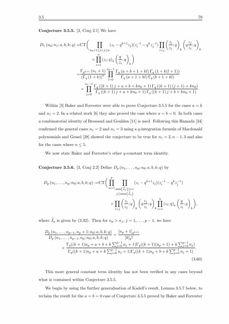
3.5 79
Conjecture 3.5.5. [3, Conj 2.1] We have
D1 (n0;n1; a, b, k; q) =CT
( ∏
n0+1≤i<j≤n
(zi − qk+1zj)(z−1i − qkz−1
j )∏
i<j
(zizj; q
)
k
(qzjzi; q
)
k
×n∏
i=1
(zi; q)a
(q
zi; q
)
b
)
=Γqk+1 (n1 + 1)
(Γq (1 + k))n
n0−1∏
l=0
Γq (a+ b+ 1 + kl) Γq (1 + k(l + 1))
Γq (a+ 1 + kl) Γq (b+ 1 + kl)
×n1−1∏
j=0
Γq ((k + 1) j + a+ b+ kn0 + 1) Γq ((k + 1) (j + 1) + kn0)
Γq ((k + 1) j + a+ kn0 + 1) Γq ((k + 1) j + b+ kn0 + 1).
Within [3] Baker and Forrester were able to prove Conjecture 3.5.5 for the cases a = k
and n1 = 2. In a related work [6] they also proved the case where a = b = 0. In both cases
a combinatorial identity of Bressaud and Goulden [11] is used. Following this Hamada [34]
confirmed the general cases n1 = 2 and n1 = 3 using a q-integration formula of Macdonald
polynomials and Gessel [28] showed the conjecture to be true for n1 = 2, n− 1, 3 and also
for the cases where n ≤ 5.
We now state Baker and Forrester’s other q-constant term identity.
Conjecture 3.5.6. [3, Conj 2.2] Define Dp (n1, . . . , np;n0; a, b, k; q) by
Dp (n1, . . . , np;n0; a, b, k; q) :=CT
( p∏
α=1
∏
min(Jα)≤i<
j≤max(Jα)
(zi − qk+1zj)(z−1i − qkz−1
j )
×∏
i<j
(zizj; q
)
k
(qzjzi; q
)
k
n∏
i=1
(zi; q)a
(q
zi; q
)
b
),
where Jα is given by (3.32). Then for np > nj, j = 1, . . . , p− 1, we have
Dp (n1, . . . , np−1, np + 1;n0; a, b, k; q)
Dp (n1, . . . , np−1, np;n0; a, b, k; q)=
[np + 1]qk+1
[k]q!
×Γq((k + 1)np + a+ b+ k
∑p−1j=0 nj + 1)Γq((k + 1)(np + 1) + k
∑p−1j=0 nj)
Γq((k + 1)np + a+ k∑p−1
j=0 nj + 1)Γq((k + 1)np + b+ k∑p−1
j=0 nj + 1).
(3.60)
This more general constant term identity has not been verified in any cases beyond
what is contained within Conjecture 3.5.5.
We begin by using the further generalisation of Kadell’s result, Lemma 3.5.7 below, to
reclaim the result for the a = b = 0 case of Conjecture 3.5.5 proved by Baker and Forrester

80 3.5
in [6]. Unlike the methods in [6] we are able to extend ours to prove the more general case
of Conjecture 3.5.6 with a = b = 0.
Lemma 3.5.7. Let J = r, . . . , r + s ⊆ 1, . . . , n and h (z) be antisymmetric with
respect to zj , j ∈ J then
CT
( ∏
r≤i<j≤r+s
(zi − azj)h (z)
)=
[s]a!
s!CT
( ∏
r≤i<j≤r+s
(zi − zj) h (z)
), (3.61)
(cf. (3.23)).
Proof. Let SJ = 〈sj : j ∈ r, . . . , r + s− 1〉 . For any permutation σ ∈ SJ , the operation
z → σz leaves the constant term on the left hand side of (3.61) unchanged. Hence
CT
( ∏
r≤i<j≤r+s
(zi − azj) h (z)
)= CT
( ∏
r≤i<j≤r+s
(zσ(i) − azσ(j)
)h (σz)
).
Since h (z) is antisymmetric h (σz) = (−1)l(σ) h (z) , summing over all permutations gives
CT
( ∏
r≤i<j≤r+s
(zi − azj)h (z)
)
=1
s!CT
(( ∑
σ∈SJ
(−1)l(σ)∏
r≤i<j≤r+s
(zσ(i) − azσ(j)
))h (z)
).
Since∏
1≤i<j≤n
(zi − azj) =∑
ω∈Sn
(−a)l(ω) zωδ
we can write
∑
σ∈SJ
(−1)l(σ)∏
r≤i<j≤r+s
(zσ(i) − azσ(j)
)=∑
σ∈SJ
(−1)l(σ) σ∑
ω∈SJ
(−a)l(ω) zωδ . (3.62)
Letting ω = σ−1 we see that the coefficient of zδ in (3.62) is∑
σ∈SJal(σ). The result
follows from the identity (3.21)
As previously stated the following result is due to Baker and Forrester [6], however
here an alternative method is used.

3.5 81
Theorem 3.5.8. We have
D1 (n1;n0; 0, 0, k; q) =Γqk+1 (n1 + 1)
(Γq (1 + k))n
n1−1∏
j=0
Γq ((k + 1) (j + 1) + kn0)
Γq ((k + 1) j + kn0 + 1)
×n0−1∏
l=0
Γq (1 + k(l + 1))
Γq (1 + kl). (3.63)
Proof. Let (I, J) = (∅, Jn0,n1) and η∗ = η∗(0n0 ;n1). By Theorem 3.4.3 we have
S(I,J)η∗ (z) = ∆Jn0,n1
t (z),
and hence
⟨S(I,J)η∗ (z), S
(I,J)η∗ (z)
⟩q,qt
= CT
( ∏
n0+1≤i<j≤n
(zi − q−kzj)(z−1i − qkz−1
j )
×∏
1≤i<j≤n
(zizj; q
)
k
(qzjzi; q
)
k
). (3.64)
To apply Lemma 3.5.7 we view (3.64) as
CT
( ∏
n0+1≤i<j≤n
(zi − q−kzj)h (z)
)
where h (z) is antisymmetric with respect to zn0+1, . . . , zn. Using Lemma 3.5.7 twice we
see that
D1 (n1;n0; 0, 0, k; q) =[n1]qk+1 !
[n1]q−k !
⟨S(I,J)η∗ (z), S
(I,J)η∗ (z)
⟩q,qt
.
From (1.51) we have[x]qk !
[x]q−k != q
k(x−1)x2 . (3.65)
Using this and (3.59) it follows that
D1 (n1;n0; 0, 0, k; q) =[n1]qk+1 ![n1 + nk]q! (1− q)n1
[k]q!n(qn1(k+1)+n0k; q−(k+1)
)n1
. (3.66)
To show (3.66) is equivalent to (3.63) we firstly use the identity [46] Γq (1 + n) = [n]q! to
show[n1]qk+1 !
[k]q!n=
Γqk+1 (n1 + 1)
(Γq (1 + k))n
andn0−1∏
l=0
Γq (1 + k(l + 1))
Γq (1 + kl)= [n0k]q!.

82 3.5
Lastly,
[n1 + nk]q! (1− q)n1
(qn1(k+1)+n0k; q−(k+1)
)n1
= [n0k]q!
n1−1∏
j=0
[(k + 1) j + kn0 + k]q!
[(k + 1) j + kn0]q!,
is seen to be true by expanding both sides and comparing terms.
Our final result in this section is proving the specialisation a = b = 0 of Conjecture
3.5.6, which until now has not been done. We do this by finding the analogue of Theorem
3.5.8 for η∗(n0,Np)and stating the result as a corollary. We begin with a generalisation of
Lemma 3.5.7.
Lemma 3.5.9. Let J ⊆ 1, . . . n = J1 ∪ . . . ∪ Js and h (z) be antisymmetric with respect
to zj, j ∈ J then
CT
( s∏
α=1
∏
min(Jα)≤i
<j≤max(Jα)
(zi − azj)h (z)
)=
s∏
α=1
[|Jα|]a!
|Jα|!CT
( s∏
α=1
∏
min(Jα)≤i
<j≤max(Jα)
(zi − zj) h (z)
).
Theorem 3.5.10. With Np as defined by (3.34) we have
Dp (Np;n0; 0, 0, k; q) =
p∏
α=1
([nα]qk+1 !
) [kn+max (NP )]q!
[k]q!n
×(1− q)max(NP )
Πmax(Np)j=1
(1− qjqk(n−m(j))
) , (3.67)
where m(j) is specified just below (3.56).
Proof. With (I, J) = (∅, Jn0,Np) and η∗ = η∗(0n0 ;Np), Theorem 3.4.3 implies
S(I,J)η∗ (z) = ∆Jn0,Np
t (z)
and hence the inner product⟨S(I,J)η∗ (z), S
(I,J)η∗ (z)
⟩q,qk
can be written as
⟨S(I,J)η∗ (z), S
(I,J)η∗ (z)
⟩q,qk
= CT
( p∏
α=1
∏
min(Jα)≤i<
j≤max(Jα)
(zi − q−kzj)(z−1i − qkz−1
j )
×∏
1≤i<j≤n
(zizj; q
)
k
(qzjzi; q
)
k
).
Applying Lemma 3.5.9 twice to (3.56) and again using (3.65) the result is obtained as in
Theorem 3.5.8.

3.6 83
The a = b = 0 case of Conjecture 3.5.6 is verified by substituting (3.67) into the left
hand side of (3.60) and making the obvious simplifications.
3.6 Further Work
The theory in this section leads most naturally to an investigation of interpolation polyno-
mials with prescribed symmetry. Since the operator Hi (2.36) satisfies the Hecke algebra
(1.12) and plays the same role in interpolation theory as Ti does in nonsymmetric Macdon-
ald polynomial theory, it seems natural to define the symmetrising and antisymmetrising
operators for the interpolation polynomials as
U+∗ :=
∑
σ∈Sn
Hσ, U−∗ :=
∑
σ∈Sn
(−1
t
)l(σ)
Hσ,
where Hσ is as in (1.5). Mirroring the work in Section 3.2 we use these operators to build
the prescribed symmetry operator O∗I,J . Explicitly we have
O∗I,J :=
∑
ω∈WI∪J
(−1
t
)l(ωJ )
Hω.
From this set up one is able derive the interpolation polynomial analogues of Proposi-
tion 3.2.1 and Proposition 3.2.2. Trial computations also suggest that it may be possible
to extend Proposition 3.3.1, Conjecture 3.4.1 and Theorem 3.4.3 to interpolation polyno-
mial theory. Trial computations suggest that the antisymmetric interpolation polynomial
S∗κ+δ(z; q, t) and the symmetric interpolation polynomial P ∗
κ (z; q, t) are closely related by
a Vandermonde-type product, however it is not immediately obvious how to transform the
parameters in each polynomial. In Section 5 we give further details of these formulas. Such
relationships are also evident between the prescribed symmetry interpolation polynomials
labelled by η∗ = η(n0;Np) or η∗ = η(Np,n0) and the corresponding symmetric interpolation
polynomial P ∗κ (z1, . . . , zn0) or P
∗κ (zn−n0−1, . . . , zn).

84 3.6

Chapter 4
Pieri-Type Formulas for
Nonsymmetric Macdonald
Polynomials
The Pieri formulas give the branching coefficients for the product of the rth elementary
symmetric function er(z) and a symmetric polynomial. The original Pieri formula con-
sidered the product between er(z) and sκ(z); more recently the Pieri formulas for the
symmetric Macdonald polynomials were obtained. Until now little work has been done on
the nonsymmetric analogues of the Pieri formulas. In this chapter we consider the product
of er(z) and Eη(z; q−1, t−1) and the closely related generalised binomial coefficients
(λη
)q,t
(2.65).
The chapter begins with a brief history on the Pieri formulas, stating the known results
and applications of the theory. The Mathematical study commences with determining
which coefficients in the expansion will be non-zero. The evaluation of the Pieri-type
coefficients for the nonsymmetric Macdonald polynomials is separated into two studies.
The first considers the expansion of e1(z)Eη(z; q−1, t−1) and the second the general Pieri-
type formulas for er(z)Eη(z; q−1, t−1). Although both studies depend heavily on the theory
of interpolation polynomials the overall approaches are quite different.
The first study is carried out by first determining the coefficients in the expansion
of ziEη(z; q−1, t−1) (Proposition 4.3.7). This result is used to compute the branching
coefficients for e1(z)Eη(z; q−1, t−1) (Proposition 4.3.8). Upon obtaining the Pieri-type
coefficients in the case r = 1 we are able to provide an evaluation of the geneneralised
binomial coefficients(λη
)q,t
in the case |λ| = |η|+1 (Proposition 4.3.13) and the Pieri-type
coefficients in the expansion of en−1(z)Eη(z; q−1, t−1) (Propositions 4.3.17 and 4.3.15). We
85

86 4.1
conclude the study with a discussion of an alternative derivation of the coefficients in the
expansion of e1(z)Eη(z; q−1, t−1).
The second study begins with another alternative derivation of the Pieri-type coef-
ficients for the case r = 1 (Proposition 4.4.1 and Corollary 4.4.2). The significance of
this alternative method is its ability to be generalised to any value of r. We provide the
structure of the general Pieri-type formulas (Theorem 4.4.4) and explicit formulas for the
coefficients (Proposition 4.4.6). As in the previous study we use the formulas for the Pieri-
type coefficients to evaluate the generalised binomial coefficients(λη
)q,t
where |λ| = |η|+ r
(Corollary 4.4.5). The study concludes with a discussion of the considered simplifications
of the formulas.
4.1 A Brief History
The Pieri formulas were first considered by Italian geometer Mario Pieri around the early
1900’s and provided a formula for expressing the product of a Schur polynomial and a
complete symmetric function hr(z) (1.7) in terms of Schur polynomials of higher degree.
Over time the Pieri formulas have evolved to consider the product of polynomials with
the elementary symmetric function er(z). The Pieri formula for Schur functions, see for
example [54], states
er(z)sκ(z) =∑
µ:µ/κ is a vertical r strip
sµ(z).
This was later generalised to the Pieri formula for symmetric Macdonald polynomials,
which can be expressed as [54, Section VI. 6]
er(z)Pκ(z; q, t) =∑
µ:µ/κ is a vertical r strip
ψµ/κ(q, t)Pµ(z; q, t) (4.1)
where ψµ/κ(q, t) is given by
ψµ/κ(q, t) := tl(µ)−l(κ)Pκ(tδ)
Pµ(tδ)
∏
1≤i<j≤n
1− qκi−κj tj−i+θi−θj
1− qκi−κj tj−i, (4.2)
and θ = µ− κ. The evaluation Pκ(tδ) is given explicitly by (3.47).
The Pieri formulas found application in studies of certain vanishing properties of Mac-
donald polynomials at tk+1qr−1 = 1 [21]. The dual of (4.1) has also found application in
the study of certain probabilistic models related to the Robinson-Schensted-Knuth corre-
sponence [26]. In 2002 Marshall [58] derived the Pieri-type coefficients in the expansion

4.2 87
of e1(z)Eη(z;α) finding the nonsymmetric Jack analogue of (4.1) in the case r = 1. Mar-
shall’s result was reclaimed by Schutzer [71] in 2004 using combinatorial methods. A
further alternate derivation of Marshall’s result and the Pieri-type coefficients in the ex-
pansion of en−1(z)Eη(z;α) can found in [24]. Most recently Pieri type formulas have been
obtained for the generalised Hall-Littlewood function [77].
4.2 Preliminaries
4.2.1 General Pieri-type formulas
We set up our study of Pieri-type formulas for the nonsymmetric Macdonald polynomials
by considering a more general situation.
If we take a linear basis of polynomials Gη(z) of degree |η|, satisfying
Gη(λ) = 0, for all |λ| ≤ |η|, λ 6= η (4.3)
and a polynomial fr(z) of degree r such that fr(η) = 0 we have
fr(z)Gη(z) =∑
|η|+1≤|λ|≤|η|+r
AηλGλ(z),
for some coefficients Aηλ. Examples of polynomials satisfying (4.3) are the interpolation
Macdonald polynomials (Section 2.2), the Schubert polynomials [50] and the interpolation
Jack polynomials (Appendix D), with the appropriate meaning of λ.
We seek the most simplified expressions for the coefficients in the expansion for the
case where fr(z) = (er(z)− er(λ)) and Gη(z) = E∗η(z; q, t). Following the strategies of [58]
we then use the fact that the top homogeneous component of E∗η(z; q, t) is Eη(z; q
−1, t−1)
to conclude that the coefficients A(r)η,λ(q, t) in
(er(z)− er(η))E∗η(z; q, t) =
∑
|η|+1≤|λ|≤|η|+r
A(r)ηλ (q, t)E
∗λ(z; q, t) (4.4)
are the same as those in
er (z)Eη
(z; q−1, t−1
)=
∑
λ:|λ|=|η|+r
A(r)ηλ (q, t)Eλ(z; q
−1, t−1). (4.5)

88 4.2
It is the relationship between (4.4) and (4.5) that allows us to use the theories of both
the nonsymmetric Macdonald polynomials and the interpolation Macdonald polynomials
to derive and simplify the coefficients A(r)ηλ (q, t).
4.2.2 Structure of Pieri-type expansions
We commence the derivation of the Pieri-type formulas for the nonsymmetric Macdonald
polynomials by determining the necessary conditions for the coefficients (4.5) to be non-
zero.
We begin using the interpolation polynomials to restrict the summation in both (4.4)
and (4.5). The extra vanishing conditions of the interpolation polynomials (Proposition
2.2.19) states that E∗η(λ; q, t) = 0 if η 6′ λ allowing us to write
(er(z)− er(η))E∗η(z; q, t) =
∑
|η|+1≤|λ|≤|η|+rη′λ
A(r)ηλ (q, t)E
∗λ(z; q, t) (4.6)
and
er(z)Eη(z; q−1, t−1) =
∑
|λ|=|η|+rη′λ
A(r)ηλ (q, t)Eλ(z; q
−1, t−1)
respectively. Following the methods of Forrester and McAnally [24] we exploit the orthog-
onality of the nonsymmetric Macdonald polynomials to identify further zero coefficients
in the expansions.
Proposition 4.2.1. We have
A(r)ηλ (q, t) = A
(n−r)λ,η+(1n)
(q−1, t−1)Nη(q, t)
Nλ(q, t), (4.7)
where Nη(q, t) and η + (kn) are given by (2.22) and (1.38) respectively.
Proof. With λ such that |λ| = |η| + r and η ′ λ by (4.5) and the orthogonality and
linearity properties of 〈·, ·〉q,t we have
⟨er(z)Eη(z; q
−1, t−1), Eλ(z; q−1, t−1)
⟩q,t
= A(r)ηλ (q, t)
⟨Eλ(z; q
−1, t−1), Eλ(z; q−1, t−1)
⟩q,t. (4.8)
Using (1.26) we can write the left hand side of (4.8) as
CT(er(z)Eη(z; q−1, t−1)Eλ(z
−1; q, t)W (z)). (4.9)

4.2 89
Replacing z with z−1 and then multiplying er(z−1) by (z1 . . . zn) and Eη(z
−1; q−1, t−1) by
(z1 . . . zn)−1 allows us to write (4.9) as
CT(en−r(z)Eη+(1n)(z−1; q−1, t−1)Eλ(z; q, t)W (z−1)),
where (2.12) has been used to simplify Eη(z−1; q−1, t−1). By again interchanging z and
z−1 we recognise this as
⟨Eη+(1n)(z; q
−1, t−1), en−r(z)Eλ(z; q−1, t−1)
⟩q,t.
After further minor manipulation, (4.8) shows this reduces to
A(n−r)λ,η+(1n)(q
−1, t−1)⟨Eη+(1n)(z; q
−1, t−1), Eη+(1n)(z; q−1, t−1)
⟩q,t.
Since Nη(q, t) = Nη(q−1, t−1) and Nη(q, t) = Nη+(1n)(q, t) it follows that (4.7) is true.
Corollary 4.2.2. We have
A(r)ηλ (q, t) = 0 if η 6′ λ or λ 6′ η + (1n),
and therefore
er(z)Eη(z; q−1, t−1) =
∑
|λ|=|η|+rη′λ′η+(1n)
A(r)ηλ (q, t)Eλ(z; q
−1, t−1). (4.10)
In [24] Forrester and McAnally gave further structure to the λ in (4.10), showing that
compositions λ satisfying η ′ λ ′ η + (1n) and |λ| = |η| + r are characterised by the
properties that there are sets i1, . . . , ir ⊂ 1, . . . , n and j1, . . . , jn−r = 1, . . . , n \
i1, . . . , ir such that
λσ(ip) = ηip + 1, for ip ≤ σ(ip), p = 1, . . . , r,
λσ(jp) = ηjp , for jp ≥ σ(jp), j = 1, . . . , n − r, (4.11)
for some defining permutation σ. By Corollary 1.4.5 a defining permutation of η ′ λ
is the inverse of a defining permutation of λ ′ η + (1n). Therefore if σ is a defining
permutation of η ′ λ we have
ηi < λσ(i), if i < σ(i), and ηi ≤ λσ(i), if i ≥ σ(i),

90 4.3
and
λσ(i) < ηi + 1, if σ(i) < i, and λσ(i) ≤ ηi + 1, if σ(i) ≥ i.
Combining these together and implementing the requirement |λ| = |η|+ r gives (4.11).
We now work towards finding the explicit formulas for the coefficients A(r)ηλ (q, t) in the
case r = 1.
4.3 Pieri-type Formulas for r = 1
In this section we provide the explicit branching coefficients for the Pieri-type formulas
for the nonsymmetric Macdonald polynomials in the case r = 1. We do this by first
considering the branching coefficients for the product ziEη(z; q−1, t−1) in terms of higher
order nonsymmetric Macdonald polynomials.
That such branching formulas can be derived is suggested by Jack polynomial the-
ory. Marshall [58] derived the branching coefficients for the products ziEη(z;α) and
e1(z)Eη(z;α) following a strategy of Knop and Sahi [45], which proceeds by exploiting
the theory of interpolation Jack polynomials.
Similarly to the Jack case, the interpolation polynomials, introduced in Section 2.2,
play a key role in deriving the branching coefficients for the product ziEη(z; q−1, t−1).
The overall strategy for finding the branching coefficients is to use the mapping Ψ
(2.41) between Eη(z; q−1, t−1) and E∗
η(z; q, t) to intertwine the actions of multiplication by
zi on Eη(z; q−1, t−1) and a certain operator Zi on E
∗η(z; q, t). Hence, by first determining
an explicit form for the coefficients Aiηλ (q, t) in the expansion
ZiE∗η(z; q, t) =
∑
λ
Aiηλ (q, t)E
∗λ(z; q
−1, t−1)
we can apply the mapping Ψ to obtain an explicit form of the coefficients of ziEη(z; q−1, t−1)
in terms of the Eλ(z; q−1, t−1) (Section 4.3.3). Using this result we can derive the explicit
formula for the expansion of e1(z)Eη(z; q−1, t−1) (Section 4.3.4). As a check on our result
we prove that the classical limit reclaims Marshall’s analogous result for nonsymmetric
Jack polynomials (Section 4.3.5). As a corollary of obtaining the Pieri-type coefficients
for the case r = 1 we evaluate the generalised binomial coefficients(λη
)q,t
in the case
|λ| = |η| + 1 (Section 4.3.6) and provide two methods for finding the Pieri-type formulas
for the case r = n − 1 (Section 4.3.7); one using the identity (2.13) and the other using
orthogonality properties.

4.3 91
A recent manuscript of Lascoux [49], available only on his website, contains results
equivalent to our propositions 4.3.7 and 4.3.8. The polynomials used in his study differ
from ours by a change of indeterminate. We conclude our study on Pieri-type formulas
for r = 1 by presenting Lascoux’s derivation (Section 4.3.8).
Before deriving the explicit formulas for the Pieri-type formulas for r = 1 we give more
structure to the sets restricting the summation in (4.10).
4.3.1 Non-zero coefficients
We denote the set of λ in the summation from (4.10), in the case r = 1, by Jλη,1, that is
Jλη,1 := λ : |λ| = |η|+ 1, η ′ λ η + (1n). (4.12)
The following proposition shows how we can write Jλη,1 in terms of λ = cI(η) by introducing
a restriction on the sets I ⊆ 1, . . . , n that ensures we never have cI(η) = cJ(η) for I 6= J .
Proposition 4.3.1. [44] Let I = t1, . . . , ts with 1 ≤ t1 < . . . < ts ≤ n and I 6= ∅. We
call I maximal with respect to η iff
(1) ηj 6= ηtu , j = tu−1 + 1, . . . , tu − 1 (u = 1, . . . , s; t0 := 0);
(2) ηj 6= ηt1 + 1, j = ts + 1, . . . , n.
We have
Jλη,1 = λ : λ = cI(η), I maximal with respect to η.
Proof. By Lemma 1.4.2 we know that any λ such that η ′ λ can be expressed as cI(η)
for some set I. It is straight forward to show that cI(η) ′ η+(1n) by taking the defining
permutation to be the inverse of that of η ′ λ; σ. It follows from (1.53) that restricting
the sets to those maximal with respect to η ensures cI(η) 6= cJ(η) for I 6= J.
For example with η = (1, 1, 1) the sets 1, 1, 2 and 1, 2, 3 are maximal and all
other subsets of 1, 2, 3 are not.
We denote the maximal sets by
JIη,1 := I : I maximal with respect to η.

92 4.3
4.3.2 The intertwining formula
In order to use the theory of the interpolation polynomials to assist in our derivation of
the branching coefficients in the product of ziEη(z; q−1, t−1) we must first introduce the
intertwining formula equation (4.14) below. This is due to Knop [44], however in the
following an alternative proof is given. The corollary after this proposition leads us nicely
to the beginnings of the derivation of the first Pieri-type formula.
Proposition 4.3.2. [44, Theorem 5.1] Define
Zi := t(n2)(ziΞi − 1)Ξ1 . . . Ξi . . .Ξn, (4.13)
where the hat superscript on Ξi denotes the absence of Ξi in the product of operators
Πnj=1Ξj. With Ψ as defined in (2.41) and M an operator which acts on the subspace of
homogeneous polynomials of degree d by multiplication with q−(d2) we have
ZiΨM = ΨMzi. (4.14)
Proof. First consider the action of Zi on E∗η(z; q, t). By the commutativity of the Ξi we
have
ZiE∗η(z; q, t) = (zi − Ξ−1
i )t−(n2)Ξ1 . . .ΞnE
∗η(z; q, t). (4.15)
Using (2.39), (2.10), then the identity Σil′η(i) =
(n2
)we can simplify (4.15) to
q−|η|(zi − ηi)E∗η(z; q, t). (4.16)
Since (4.16) vanishes for all z = λ, |λ| ≤ |η| and has degree |η|+ 1 we must have
ZiE∗η(z; q, t) = q−|η|
∑
λ:|λ|=|η|+1
Aiηλ (q, t)E
∗λ(z; q, t), (4.17)
for some coefficients Aiηλ (q, t) ∈ Q(q, t). Equating the leading terms of (4.16) and the right
hand side of (4.17) using Theorem 2.2.8 gives
ziEη(z; q−1, t−1) =
∑
λ:|λ|=|η|+1
Aiηλ (q, t)Eλ(z; q
−1, t−1). (4.18)

4.3 93
Applying the action of ΨM to both sides of (4.18) and using (2.41) shows
ΨMziEη(z; q−1, t−1) = q−
(|η|+12
) ∑
λ:|λ|=|η|+1
Aiηλ (q, t)E
∗λ(z; q, t). (4.19)
Using (4.17) and the identity (x+ 1
2
)− x =
(x
2
)
the right hand side of (4.19) can be simplified to
q−(|η|2
)ZiE
∗η(z; q, t). (4.20)
By recalling the action of M and again using (2.41) we obtain
ΨMziEη(z; q−1, t−1) = ZiΨMEη(z; q
−1, t−1).
Finally, since the Eη(z; q−1, t−1) form a basis for analytic functions in zη it follows
that the intertwining property (4.14) holds generally.
Corollary 4.3.3. We have
ziEη(z; q−1, t−1) = q|η|Ψ−1ZiE
∗η(z; q, t).
Proof. Follows from (4.19) and (4.20).
4.3.3 The product ziEη
The previous corollary indicates that the next step towards finding the decomposition of
ziEη(z; q−1, t−1) is to determine an explicit formula for ZiE
∗η(z; q, t). The latter can be
deduced as a corollary of the following lemma, specifying the expansion of (ziΞi − 1)f(z),
where according to (2.35) ziΞi − 1 := Hi . . . Hn−1Φ∗qH1 . . . Hi−1.
Lemma 4.3.4. Let Zi = Hi . . . Hn−1Φ∗qH1 . . . Hi−1. The action of Zi on f(z) is given by
Zif(z) =∑
I⊆1,...,ni∈I
riI (z)f(Iz).
Here the rational function riI (z) can be expressed as
riI (z) = χ
iI (z)AI(z)BI(z), (4.21)

94 4.3
where
I =t1, . . . , ts, 1 ≤ t1 < . . . ts ≤ n, (4.22)
AI(z) = a(ztsq, zt1
) s−1∏
u=1
a(ztu , ztu+1), (4.23)
BI(z) =(zts − t−n+1)
t1−1∏
j=1
b(ztsq, zj
)
×s∏
u=1
tu+1−1∏
j=tu+1
b(ztu , zj), ts+1 := n+ 1, (4.24)
χiI (z) =
1a(ztk−1
,zi), i = tk, k = 2, . . . , s
1a(
ztsq
,zi), i = t1,
(4.25)
and Iz is defined as
(Iz)i =
ztu−1 , i = tu, if u = 2, . . . , s
zts/q, i = t1
zi , i /∈ I.
(4.26)
The quantities a(x, y) and b(x, y) are defined in (4.27) below.
Proof. Using (2.36) the action of Hi on f(z) can be expressed as
Hif(z) = a(zi, zi+1)f(z) + b(zi, zi+1)sif(z),
where
a(x, y) :=(t− 1)x
x− y, b(x, y) :=
x− ty
x− y. (4.27)
Hence Zi can be written as
(a(zi, zi+1) + b(zi, zi+1)si) . . . (a(zn−1, zn) + b(zn−1, zn)sn−1)
× Φ∗q(a(z1, z2) + b(z1, z2)s1) . . . (a(zi−1, zi) + b(zi−1, zi)si−1). (4.28)
Let
KiI := si . . . str+1−1 . . . sts−1 . . . sn−1∆s1 . . . st1 . . . str−1 . . . si−1, for i ∈ I,

4.3 95
where 1 ≤ t1 < . . . < tr = i < tr+1 < . . . < ts ≤ n, the hat superscript denotes the absence
of the corresponding operators and I as defined in the statement of the result. It is clear
that the expansion of Zi will be of the form
Zi =∑
I⊆1,...,ni∈I
riI (z)K
iI
for coefficients riI (z) involving a(x, y) and b(x, y). Further, it is easily verified that
KiI f(z) = f(Iz). The coefficients r
iI (z) are found by considering the individual terms in
the expansion of (4.28). Due to the need to commute the transposition operators si through
to the right the final formula is more simply obtained by expanding (4.28) termwise from
the right. Inevitably, the exercise is rather tedious, however it can be structured somewhat
by considering four disjoint classes of sets I
I1 = i,
I2 = . . . , i,
I3 = i, . . .,
I4 = . . . , i, . . .,
which exhaust all possibilities. This cataloguing allows the coefficients of the corresponding
four forms of KiI to be considered separately and the result is more easily observed.
Explicitly, the four forms of KiI are
KiI1
= si . . . sn−1∆s1 . . . si−1,
KiI2
= si . . . sn−1∆s1 . . . st1 . . . str−1 . . . si−1,
KiI3
= si . . . str+1−1 . . . sts−1 . . . sn−1∆s1 . . . si−1,
KiI4
= si . . . str+1−1 . . . sts−1 . . . sn−1∆s1 . . . st1 . . . str−1 . . . si−1.
In relation to KI2 , KI4 the coefficient of s1 . . . st1 . . . str−1 . . . si−1 in the partial expansion,
that is terms to the right of Φ∗q, in (4.28) is
a(z1, zt1+1)
r−2∏
u=1
a(ztu+1, ztu+1+1)
t1−1∏
j=1
b(z1, zj+1)
r−1∏
u=1
tu+1−1∏
j=tu+1
b(ztu+1, zj+1).

96 4.3
Hence the coefficient of ∆s1 . . . st1 . . . str−1 . . . si−1 will be
(zn − t−n+1)a(znq, zt1
) r−2∏
u=1
a(ztu , ztu+1)×t1−1∏
j=1
b(znq, zj
) r−1∏
u=1
tu+1−1∏
j=tu+1
b(ztu , zj).
Similarly, for KI1 , KI3 , the coefficient of s1 . . . si−1 and ∆s1 . . . si−1 are respectively
i−1∏
j=1
b(z1, zj+1)
and
(zn − t−n+1)i−1∏
j=1
b(znq, zj
).
The final coefficients rIj(z) are found by continuing the expansion of (4.28) from the right
and considering the four forms of KI separately. Thus we find that
riI1
(z) =AI(z)BI(z)
a(ziq , zi)
riI2
(z) =AI(z)BI(z)
a(ztr−1 , ztr )
riI3
(z) =AI(z)BI(z)
a(ztsq , zt1)
riI4
(z) =AI(z)BI(z)
a(ztr−1 , ztr ),
where AI(z) and BI(z) are defined by (4.23) and (4.24), respectively. After recalling the
definition of χiI (z) given above, the sought explicit formula (4.21) follows.
Corollary 4.3.5. We have
ZiE∗η(z; q, t) = q−|η|ηi
∑
I⊆1,...,ni∈I
riI (z)E∗
η (Iz; q, t). (4.29)
Proof. Follows after recalling (4.13).
Together Proposition 4.3.2 and Corollary 4.3.5 allow us to derive an initial expansion
of ziEη(z; q−1, t−1) in terms of the Macdonald polynomials of degree |η|+ 1.
Proposition 4.3.6. We have
ziEη(z; q−1, t−1) = ηiq
−|η|∑
|λ|=|η|+1
∑
I⊆1,...,ni∈I
riI (λ)E∗
η(Iλ; q, t)
E∗λ(λ; q, t)
Eλ(z; q−1, t−1). (4.30)

4.3 97
Proof. By the vanishing properties of the interpolation polynomials, when the right hand
sides of (4.17) and (4.29) are equated and evaluated at z = λ we obtain
Aiλη (q, t) = ηi
∑
I⊆1,...,ni∈I
riI (λ)E∗
η(Iλ; q, t)
E∗λ(λ; q, t)
.
Substituting this back into (4.17) and applying Corollary 4.3.3 gives (4.30).
The formula (4.30) can be improved as follows.
Proposition 4.3.7. Let
BI(z) := (qzt1 − t−n+1)
n∏
j=ts+1
b(qzt1 , zj)
s∏
u=1
tu−1∏
j=tu−1+1
b(ztu , zj), (4.31)
t0 := 0 and
χiI (z) :=
zia(zi,ztk+1
) , i = tk, k = 1, . . . , s − 1
zia(zi,qzt1)
, i = ts,
where I = t1, . . . , ts ⊆ 1, . . . , n, with 1 ≤ t1 < . . . < ts ≤ n and I 6= ∅. We have
ziEη(z; q−1, t−1) =
∑
I∈JIη , i∈I
cI(η)=λ
χiI (η)AI(η)BI(η)kη
kcI(η)EcI(η)(z; q
−1, t−1). (4.32)
Proof. By the definition of Iz (4.26) we have E∗(Iλ) 6= 0 if and only if cI(η) = λ. Therefore
by Proposition 4.3.1 we can restrict the summation in (4.30) to I ∈ JIη , giving
ziEη
(z; q−1, t−1
)= ηi
∑
I∈JIη , i∈I
cI(η)=λ
riI
(cI (η)
)E∗
η (η)
E∗cI(η)
(cI (η)
) EcI(η)
(z; q−1, t−1
). (4.33)
It can be seen that for I maximal with respect to η we have χiI (η) = ηiχ
iI (cI(η)) and
BI(cI(η)) = BI(η). Since AI(cI(η)) = AI(η), it follows that
ηiriI (cI(η)) = χ
iI (η)AI(η)BI(η). (4.34)
By substituting (4.34) into (4.33) and making use of the evaluation formula (2.55) we
arrive at our final decomposition (4.32).

98 4.3
4.3.4 The main result
Using Proposition 4.3.7 we now provide an explicit formula for the coefficients A(1)ηλ (q, t)
in (4.5).
Proposition 4.3.8. We have
e1(z)Eη(z; q−1, t−1) =
∑
I∈JIη
A(1)η,cI(η)
(q, t)EcI (η)(z; q−1, t−1), (4.35)
where A(1)η,cI (η)
(q, t) is defined by
A(1)η,cI (η)
(q, t) :=(1− q)d′η(q
−1, t−1)AI(η)BI(η)
qηt1+1(t− 1)d′cI (η)(q−1, t−1)
. (4.36)
Proof. Summing (4.32) over all i and then reversing the order of summation gives
e1(z)Eη(z; q−1, t−1) =
∑
I∈JIη
∑
i∈I
χiI (η)AI(η)BI(η)kη
kcI(η)EcI(η)(z; q
−1, t−1). (4.37)
We have∑
i∈I
χiI (η) =
ηt1(1− q)
(t− 1)(4.38)
and analogous to (2.62) we have
kηkcI(η)
=d′η(q
−1, t−1)
q2ηt1+1t−l′η(t1)d′cI (η)(q−1, t−1)
. (4.39)
Substituting (4.38) and (4.39) into (4.37) gives the required result.
4.3.5 The classical limit
We provide a check on our formula by showing how the classical limit of Proposition 4.3.8
reclaims the Pieri-type formula for the nonsymmetric Jack polynomial [58].
Proposition 4.3.9. We have
e1(z)Eη(z;α) =∑
I∈JIη
A(1)η,cI(η)
(α)EcI (η)(z;α),
where
A(1)η,cI (η)
(α) =−αd′η(α)Aα,I (η
α/α)Bα,I(ηα/α)
d′cI(η)
(α). (4.40)

4.3 99
The quantities in (4.40) are specified by
Aα,I(z) :=a(zts − 1, zt1)
s−1∏
u=1
a(ztu , ztu+1) (4.41)
Bα,I(z) :=(zt1 + 1 + (n− 1)/α)n∏
j=ts+1
b(zt1 + 1, zj)
×s∏
u=1
tu−1∏
j=tu−1+1
b(ztu , zj), t0 := 0 (4.42)
with
a(x, y) :=1
α(x− y), b(x, y) :=
x− y − 1/α
x− y
and
d′η(α) :=∏
(i,j)∈η
(α(aη(i, j) + 1) + lη(i, j)), (4.43)
where aη(i, j) and lη(i, j) are defined by (1.6) and (1.40) and I by (4.22). The eigenvalue
ηα is defined in Appendix C.
Proof. Our task is to show that
limt=q1/α, q→1
A(1)η,cI (η)
(q, t) = A(1)η,cI(η)
(α). (4.44)
Comparing (1.41) with (4.43), it is immediate that
limt=q1/α, q→1
(1− q)d′η(q−1, t−1)
qηt1+1(t− 1)d′cI (η)(q−1, t−1)
= −αd′η(α)
d′cI (η)(α).
To proceed further, note from (4.27) and (4.3.9) that
limt=q1/α, q→1
a(qmtn, qm′tn
′) = a(m+ n/α,m′ + n′/α)
and
limt=q1/α, q→1
b(qmtn, qm′tn
′) = b(m+ n/α,m′ + n′/α).
Using a term-by-term comparison of (4.23) and (4.31) with (4.41) and (4.42) also allows
us to conclude that
limt=q1/α, q→1
AI(η) = Aα,I(η/α)
and
limt=q1/α, q→1
BI(η) = Bα,I(η/α).

100 4.3
This establishes (4.44), thus exhibiting Proposition 4.3.9 as a corollary of Proposition
4.3.8. stuff
We now show how Proposition 4.3.8 can be used to obtain an evaluation for the gen-
eralised binomial coefficient(λη
)q,t.
4.3.6 Pieri-type formula for r = 1 and the generalised binomial coeffi-
cient
The following Lemma, due to Lascoux [49], shows how the Pieri-type coefficients A(1)ηλ (q, t)
relate to the generalised binomial coefficients(λη
)q,t
(2.65).
Lemma 4.3.10. [49] We have
(z1 + . . . + zn − |η|)E∗η(z; q, t) =
∑
λ:|λ|=|η|+1λ=cI(η)
(∣∣λ∣∣− |η|)E∗
η(λ; q, t)
E∗λ(λ; q, t)
E∗λ(z; q, t), (4.45)
where |η| = Σiηi.
Proof. The left hand side of (4.45) is a polynomial of degree |η| + 1, and vanishes for
every υ with |υ| ≤ |η|, where the linear factor implies vanishing at η. The right hand
side therefore belongs to the span of E∗λ(z) with |λ| = |η| + 1. The coefficients are found
by evaluating both sides at λ. Using Proposition 2.2.18 we restrict the summation to
successors of η.
Corollary 4.3.11. We have
(z1 + . . .+ zn)Eη(z; q−1, t−1) =
∑
λ:|λ|=|η|+1λ=cI(η)
(λ
η
)
q,t
(∣∣λ∣∣− |η|)kηkλ
Eλ(z; q−1, t−1). (4.46)
Proof. By Proposition 2.2.17 and (2.65) we have
E∗η(λ; q, t)
E∗λ(λ; q, t)
=
(λ
η
)
q,t
kηkλ.
The final result is obtained by employing Theorem 2.2.8.
Alternatively, Baker and Forrester [7] use the following generating function to relate
(4.35) to the generalised binomial coefficients.
Eη(z; q−1, t−1)
n∏
i=1
1
(zi; q)∞=∑
λ
(λ
η
)
q,t
tl(λ)−l(η) d′η(q, t)
d′λ(q, t)Eλ(z; q
−1, t−1), (4.47)

4.3 101
where (zi; q)∞ is given by (A.3).
By equating the homogeneous terms of degree |η|+ 1 in (4.47) we have
(z1 + . . .+ zn)Eη(z; q−1, t−1) =
∑
|λ|=|η|+1
(λ
η
)
q,t
tl(λ)−l(η)(1− q)d′η(q, t)
d′λ(q, t)Eλ(z; q
−1, t−1).
(4.48)
The detailed derivation of (4.47) and (4.48) would require theory not relevant to the main
concepts contained in this thesis so we rely on (4.46) to avoid having to give such a
derivation. However it is worthwhile to check that (4.46) and (4.48) are consistent. Note
that by the vanishing conditions of the interpolation polynomials we have(λη
)q,t
= 0 for
|λ| = |η|+1 if λ is not a successor of η and hence when proving that (4.46) and (4.48) are
consistent we only need to consider the successors of η.
Proposition 4.3.12. Let λ be a successor of η, then we have
(∣∣λ∣∣− |η|)kηkλ
=tl(λ)−l(η)(1− q)d′η(q, t)
d′λ(q, t). (4.49)
Proof. Using (2.55) and rearranging we rewrite (4.49) as
d′λ(q, t)d′η(q
−1, t−1)
tl(λ)−l(η)d′λ(q−1, t−1)d′η(q, t)
=(1− q)Πn
i=1λλi
i
(∣∣λ∣∣− |η|)Πn
i=1ηηii
. (4.50)
Using the second equation in (1.50) we can rewrite the left hand side of (4.50) as
1
tl(λ)−l(η)(−1)|λ|−|η| q
Σs∈λ(aλ(s)+1)tl(λ)
qΣs∈η(aη(s)+1)tl(η)= −qηt1+1.
We also have∣∣λ∣∣− |η| = (cI(η))ts − ηt1 = (q − 1)ηt1 (4.51)
andΠn
i=1λλi
i
Πni=1η
ηii
= ηt1qηt1+1.
Substituting these into the right hand side of (4.50) and appropriately cancelling completes
the proof.
By (4.46) and (4.48), on obtaining the Pieri-type formula for r = 1 we are naturally
lead to finding an explicit formula for(λη
)q,t
when |λ| = |η|+ 1.

102 4.3
Proposition 4.3.13. Suppose |λ| = |η|+ 1. Then
(λ
η
)
q,t
= −AI(η)BI(η)
(t− 1),
where λ = cI(η). If there is no such I such that λ = cI(η) then(λη
)q,t
= 0.
Proof. A comparison of (4.48) with (4.36) gives
(λ
η
)
q,t
=d′η(q
−1, t−1)d′λ(q, t)AI(η)BI(η)
d′η(q, t)d′λ(q
−1, t−1)qηt1+1(t− 1)tl(λ)−l(η). (4.52)
The final result is obtained by appropriately using the second formula from (1.50) to
reduce (4.52).
Comparing (2.65) with (4.3.13) and making use of (2.55) gives a new evaluation formula
for E∗η(λ) where |λ| = |η|+ 1.
Corollary 4.3.14. Suppose |λ| = |η|+ 1. Then
E∗η(λ; q, t) = −
AI(η)BI(η)kη(t− 1)
where λ = cI(η). If there is no such I such that λ = cI(η) then E∗η(λ; q, t) = 0.
4.3.7 The Pieri-type formula for r = n− 1
In this section we provide two explicit formulas for the coefficients A(n−1)ηλ (q, t) in (4.5).
For the first we manipulate e1(z)Eη(z; q−1, t−1) using the identity (2.13).
Proposition 4.3.15. With η′ := η − (min(η)n) we have
en−1(z)Eη(z; q−1, t−1) =
∑
I∈JIλ
A(1)λ,cI(λ)
(q−1, t−1)Eν+(min(η)n)(z; q−1, t−1), (4.53)
where A(1)λ,cI(λ)
(q, t) is defined by (4.36),
λ := (−η′ + (max(η′)n))R and ν := −cI(λ)R + ((max(λ) + 1)n). (4.54)
Proof. By Proposition 4.3.8 we have
e1(z)Eλ(z; q−1, t−1) =
∑
I∈JIλ
A(1)λ,cI(λ)
(q, t)EcI(λ)(z; q−1, t−1).
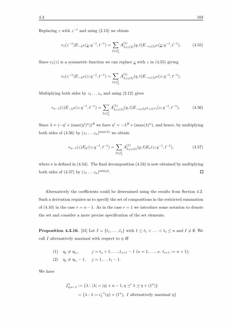
4.3 103
Replacing z with z−1 and using (2.13) we obtain
e1(z−1)E−λR(z; q−1, t−1) =
∑
I∈JIλ
A(1)λ,cI(λ)
(q, t)E−cI(λ)R(z; q−1, t−1). (4.55)
Since e1(z) is a symmetric function we can replace z with z in (4.55) giving
e1(z−1)E−λR(z; q−1, t−1) =
∑
I∈JIλ
A(1)λ,cI(λ)
(q, t)E−cI(λ)R(z; q−1, t−1).
Multiplying both sides by z1 . . . zn and using (2.12) gives
en−1(z)E−λR(z; q−1, t−1) =∑
I∈JIλ
A(1)λ,cI(λ)
(q, t)E−cI (λ)R+(1n)(z; q−1, t−1). (4.56)
Since λ = (−η′ +(max(η′)n))R we have η′ = −λR +(max(λ)n), and hence, by multiplying
both sides of (4.56) by (z1 . . . zn)max(λ) we obtain
en−1(z)Eη′(z; q−1, t−1) =
∑
I∈JIλ
A(1)λ,cI(λ)
(q, t)Eν(z; q−1, t−1), (4.57)
where ν is defined in (4.54). The final decomposition (4.53) is now obtained by multiplying
both sides of (4.57) by (z1 . . . zn)min(η).
Alternatively the coefficients could be determined using the results from Section 4.2.
Such a derivation requires us to specify the set of compositions in the restricted summation
of (4.10) in the case r = n− 1. As in the case r = 1 we introduce some notation to denote
the set and consider a more precise specification of the set elements.
Proposition 4.3.16. [24] Let I = t1, . . . , ts with 1 ≤ t1 < . . . < ts ≤ n and I 6= ∅. We
call I alternatively maximal with respect to η iff
(1) ηj 6= ηtu , j = tu + 1, . . . , tu+1 − 1 (u = 1, . . . , s; ts+1 := n+ 1);
(2) ηj 6= ηts − 1, j = 1, . . . t1 − 1.
We have
Jλη,n−1 := λ : |λ| = |η|+ n− 1, η ′ λ η + (1n)
= λ : λ = c−1I (η) + (1n), I alternatively maximal η

104 4.3
Proof. We first observe η ′ cI(η) implies c−1I (η) ′ η, and hence c−1
I (η)+(1n) ′ η+(1n).
By taking the inverse of the defining permutation of c−1I (η) ′ η+(1n) we obtain a defining
permutation for η ′ cI(η) + (1n). Therefore
Jλη,n−1 = λ : λ = c−1I (η) + (1n), I maximal with respect to c−1
I (η).
The final result is obtained from the definitions of maximal and alternatively maximal.
We denote the alternatively maximal sets by
JIη,n−1 := I : I alternatively maximal with respect to η.
For simplicity we let the symbol cI(η) denote c−1I (η) + (1n) and note the explicit formula
(cI(η))j =
ηts , j = t1
ηtu−1 + 1 , j = tu, if u = 2, . . . , s
ηj + 1 , j /∈ I.
By the definitions of the compositions cI(η) and cI(η) it can be seen that they are
related according to
η + (1n) = cI(λ), with I ∈ JIλ,1 iff λ = cI(η), with I ∈ JIη,n−1.
We can now show how Proposition 4.2.1 can be used to derive the Pieri-type coefficients
in the case r = n− 1 from the case r = 1.
Proposition 4.3.17. We have
en−1(z)Eη(z; q, t) =∑
I∈JIη,n−1
A(1)cI(η),η+(1n)(q, t)
Nη
NcI(η)EcI(η)(z; q, t), (4.58)
where A(1)cI(η),η+(1n)(q, t)(Nη/NcI(η)) can be rewritten to read
(1− q)AI(η)BI(η + (1n))(ηtsqtn − 1)dcI (η)(q
−1, t−1)
qηt1+1(t− 1)(ηtsqtn − t)dη+(1n)(q−1, t−1)
. (4.59)

4.3 105
Proof. The initial form (4.58) follows immediately from Propositions 4.2.1 and 4.3.16.
Using (4.36) and (2.22) we write the branching coefficients as
(1− q)d′cI(η)(q−1, t−1)AI(cI(η))BI(cI(η))
qηt1+1(t− 1)d′η+(1n)(q−1, t−1)
d′η(q, t)eη(q, t)
dη(q, t)e′η(q, t)
dcI(η)(q, t)e′cI (η)
(q, t)
d′cI(η)(q, t)ecI (η)(q, t). (4.60)
To reduce (4.60) to its simplest form we require the following 3 simplifications. First,
by recalling Nη(q, t) = Nη(q−1, t−1) = Nη+(1n)(q
−1, t−1) we can replace Nη(q, t) with
Nη+(1n)(q−1, t−1) and NcI(η)(q, t) with NcI(η)(q
−1, t−1). After making the obvious cancel-
lations we obtain
(1− q)AI(cI(η))BI(cI(η))
qηt1+1(t− 1)
dcI(η)(q−1, t−1)eη+(1n)(q
−1, t−1)e′cI(η)(q−1, t−1)
dη+(1n)(q−1, t−1)ecI(η)(q−1, t−1)e′η+(1n)(q
−1, t−1).
Secondly, using Lemmas 1.3.1, 1.3.3, 1.3.2 and 1.3.4 we can simplify the ratios involving
eη and e′η to
e′η+(1n)(q−1, t−1)
e′cI(η)(q−1, t−1)
= 1− (ηtsqtn−1)−1
andeη+(1n)(q
−1, t−1)
ecI(η)(q−1, t−1)
= 1− (ηtsqtn)−1.
We recall from Proposition 4.3.7 that BI(cI(λ)) = BI(λ) and AI(cI(λ)) = AI(λ). Lastly,
replacing AI(η + (1n)) with AI(η) gives (4.59).
Due to the different forms of expansions, en−1(z)Eη(z; q−1, t−1) and en−1(z)Eη(z; q, t),
and the different sets they are summed over, I ∈ JIν,1 and I ∈ JIη,n−1 it is not practical to
compare the two forms. Both derivations are included to display the different strengths
of the theory derived so far.
4.3.8 Lascoux’s derivation of the Pieri-type formula for r = 1
We conclude our initial study with an outline of the alternative derivation of the Pieri-
type coefficients in the case r = 1 provided by Lascoux. Lascoux’s result was obtained
independently and posted on his website [49] just prior to the publication [9] contain-
ing Proposition 4.3.8. Lascoux’s approach involves an interpolation polynomial slightly
different from those introduced in Section 2.2. We begin with the introduction of the
interpolation polynomials used by Lascoux.

106 4.3
Lascoux defines a new vector 〈η〉 := (〈η〉1 , . . . , 〈η〉n), where 〈η〉i is given by
〈η〉i := qηitl′η(i),
(cf. (2.10)) and a new polynomial Mη(z) satisfying Mη(〈λ〉) = 0 for all λ where |λ| ≤ |η|,
λ 6= η, having leading term zηq−Σi
(ηi2
)(cf. (1.56)). It follows that
Mη(z) = q−Σi
(ηi2
)t(n−1)|η|E∗
η(zt1−n).
By writing
(z1 + . . .+ zn − |〈η〉|)Mη(z) =∑
λ:|λ|=|η|+1λ=cI(η)
A′(1)ηλ (q, t)Mλ(z), (4.61)
where |〈η〉| := Σi 〈η〉i, and evaluating at 〈λ〉 Lascoux expresses the coefficients A′(1)ηλ (q, t)
as
A′(1)ηλ (q, t) =
(|〈λ〉| − |〈η〉|)Mη(〈λ〉)
Mλ(〈λ〉).
Lascoux finds the explicit formula of Mη(〈λ〉)/Mλ(〈λ〉) to be
Mη(〈λ〉)
Mλ(〈λ〉)= t1−nδ′(η, λ)β′(η, λ). (4.62)
In (4.62) δ′(η, λ) is given by
δ′(η, λ) :=1
1− t
∏
i
1− t
〈λ〉i 〈η〉−1i − 1
,
where the product is over all i such that 〈λ〉i 6= 〈η〉i and β′(η, λ) is defined to be
β′(η, λ) :=∏ (X ′(i, j) − t)(tX ′(i, j) − 1)
(X ′(i, j) − 1)2,
with the product over all i < j such that λi < λj and 〈λ〉i , 〈λ〉j is a subword of 〈λ〉 but
not of 〈Φη〉 and X ′(i, j) := 〈λ〉j 〈λ〉−1i .
Lascoux’s proof of (4.62) uses the fact that each successor λ can be recursively gener-
ated from η according to si, . . . , sjΦη, where si, . . . , sj is a subword of one of sn−1 . . . s1,
sn−2 . . . s1s0, . . ., s0sn−1 . . . s2, where here s0 acts on compositions and is defined by
s0 := Φs1Φ−1. He proves the equality inductively by showing the two sides are invariant

4.4 107
under the action of Φ∗q and the constants appearing in (2.53) correspond the the varia-
tion of δL(η, λ)βL(η, λ) under the action of H1, . . . ,Hn−1. Lascoux’s use of the recursive
generation of successors to prove the result inspired an alternative derivation of the eval-
uation of the ratio E∗η(λ)/E
∗λ(λ) and also gave hope to the possibility of deriving explicit
formulas for the Pieri-type coefficients for general r. With that said, we move onto our
second study.
4.4 The General Pieri-Type Formulas
In this section we provide the explicit branching coefficients for the general Pieri-type
formula, the products er(z)Eη(z; q−1, t−1). As in the previous study the coefficients are
obtained via the exploitation of the theory of the interpolation Macdonald polynomials.
We see from (4.45) and (4.61) that the key to providing explicit formulas for the
coefficients A(1)ηλ (q, t) is evaluating
E∗η(λ; q, t)
E∗λ(λ; q, t)
. (4.63)
We begin this study with a further alternative derivation of the Pieri-type formulas
for r = 1 by first evaluating (4.63) (Section 4.4.1). We then proceed with the general
formulas and their connection to the generalised binomial coefficients(λη
)q,t
(Section 4.4.2).
Following this we consider the possible simplifications of the coefficient formulas (Section
4.4.3) and then show how the results contained in Section 4.4.2 can be used to reclaim
the Pieri formulas for the symmetric Macdonald polynomial (Section 4.4.4). We complete
the chapter on Pieri-type formulas with suggestions of further work relating to the study
(Section 4.5).
4.4.1 An alternative derivation of the Pieri-type formulas for r = 1
To derive an explicit formula for (4.62) Lascoux uses the fact that successors can be
recursively generated by si and Φ, however he does not use the sequence specified by
Proposition 1.4.1. Here we show how using this specific derivation it is possible make
use of the interpolation polynomials eigenoperator properties to derive an explicit form of
(4.63).
We begin in a similar way to Lemma 4.3.4.

108 4.4
Proposition 4.4.1. With I = t1, . . . , ts maximal with respect to η, λ = cI(η) and
E∗η(z) := E∗
η(z; q, t) we have
E∗η(λ)
E∗λ(λ)
=δ(η, I)β(η, I)
qηt1 (1− t), (4.64)
where
δ(η, I) :=
s∏
u=1
t− 1
1− λtuη−1tu
and
β(η, I) :=∏
i
(1− tX(i))(t −X(i))
(1−X(i))2, (4.65)
with X(i) := ηiη−1tu(i)
, where tu(i) is the first element in I above i and if i > ts then
ηtu(i) = qηt1 . The product (4.65) is over all i 6∈ I with ηi > ηtu(i).
Proof. We first show that
Ht1 . . . Hn−1Φ∗qH1 . . . Ht1−1E
∗η(λ) =
δ(η, I)β(η, I)(1 − λt1η−1t1 )
qηt1 (t− 1)E∗
η(λ). (4.66)
With I maximal with respect to η, Proposition 1.4.1 can be used to show the polynomial
E∗λ(z) occurs exactly once in the expansion of
Ht1 . . . Hn−1Φ∗qH1 . . . Ht1−1E
∗η(z). (4.67)
Since all polynomials E∗ν(z) appearing in the full expansion of (4.67) are of size |η|+1, by
the vanishing properties of the interpolation polynomial, evaluating (4.67) at λ will reduce
it to some multiple of E∗λ(λ).
We begin by expanding (4.67) from the right using the recursive generation formulas
to determine the coefficient of each E∗λ(j)(z), where λ(j) represents the transformed η after
the jth step in the transformation from η to λ. Since the operators Hi and Φ∗q commute
through constants we consider the coefficient contribution of each operator on the E∗λ(j)(z)
to observe the result more easily. First consider the expansion of
H1 . . . Ht1−1E∗η(z).
We know from Proposition 1.4.1 that we require the si to act on η at every stage to move
ηt1 to the first position before acting upon by Φ∗q. Therefore we must take the coefficient
of E∗siλ(t1−i)(z) when Hi acts on each E∗
λ(t1−i)(z). At each stage the switching operator
swaps ηi with ηt1 , where i runs from t1− 1 to 1. By (2.53) the coefficient contribution will

4.4 109
be 1 if ηi < ηt1 , and(1− tX(i))(t −X(i))
(1−X(i))2
where X(i) = ηiη−1t1 if ηi > ηt1 . Multiplying these terms together gives the coefficient of
E∗λ(t1−1)(z) where
λ(t1 − 1) = (ηt1 , η1, . . . , ηt1−1, ηt1+1, . . . ., ηn).
Next we act upon H1 . . . Ht1−1E∗η(z) with Φ∗
q. By (2.54) when Φ∗q acts on E∗
λ(t1−1)(z)
the coefficient contribution is q−ηt1 and the new polynomial is E∗λ(t1)
(z) where
λ(t1) = (η1, . . . , ηt1−1, ηt1+1, . . . ., ηn, ηt1 + 1).
We proceed by considering the coefficients of E∗λ(j) for j > t1 in the expansion of
Ht1 . . . Hn−1E∗λ(t1)
(z).
At this stage particular attention must be payed to the set I to know whether we want to
extract the coefficient and polynomial of E∗λ(t1+j)(z) or E
∗sn−jλ(t1+j)(z) from the action of
Hn−j on E∗λ(t1+j)(z). First consider the action of Hi−1 for i ∈ I, i > t1. From Proposition
1.4.1 we know that if i ∈ I we do not require the switch si−1 in the generation of λ.
Therefore, when Hi−1 acts on E∗λ(t1+n−i+1)(z), we take the coefficient of E∗
λ(t1+n−i+1)(z).
By (2.53) this is given byt− 1
1− δ−1i−1,λ(t1+n−i+1)
.
To determine the value of δ−1i−1,λ(t1+n−i+1) we consider the (i−1)th and ith value of λ(t1+n−
i+1). Since we do not need to swap the components we must have λ(t1+n− i+1)i = λi.
Also, at this stage λ(t1 + n − i + 1)i−1 is equal to ηi since the (i − 1)th component
hasn’t changed since λ(t1). Hence the coefficient of the polynomial E∗λ(t1+n−i+1)(z) in
Hi−1E∗λ(t1+n−i+1)(z) with i ∈ I is
t− 1
1− λiη−1i
. (4.68)
It is important to note here that λi 6= ηi for i ∈ I since even if λi = ηi we would still have
λi = ηi/t. The total contribution of these terms is the product of (4.68) as i runs from 2
to s.
Lastly we consider the case where i 6∈ I, where in the expansion of Hi−1E∗λ(t1+n−i+1)(z)
we take the coefficient of the E∗si−1λ(t1+n−i+1)(z). For i > ts we use si−1 to move ηt1 + 1
to the tths position, each time swapping ηt1 +1 with ηi. For t1 < i < ts each si−1 is used to

110 4.4
move ηtu(i) to the tthu−1 position, swapping ηi and ηtu(i), where tu(i) is defined above. By
(2.53) when either ηi > ηt1 + 1, for j = ts + 1, . . . , n or ηi > ηtu(i), for t1 < i < ts we have
the coefficient(1− tX(i))(t −X(i))
(1−X(i))2
where X(i) = ηiη−1tu(i)
. Combining all coefficients gives (4.66). By (2.35) and (2.39) we
have
(zt1η−1t1 − 1)E∗
η(z) = Ht1 . . . Hn−1Φ∗qH1 . . . Ht1−1E
∗η(z). (4.69)
By (4.66) and the vanishing properties of the interpolation polynomials, evaluating (4.69)
at λ gives (4.64).
Corollary 4.4.2. We have
e1(z)Eη(z; q−1, t−1) =
∑
λ:λ=cI(η)
(|λ| − |η|)δ(η, I)β(η, I)
qηt1 (1− t)Eλ(z; q
−1, t−1). (4.70)
Of course we would like to show that the coefficients found in (4.70) are consistent
with (4.35).
Proposition 4.4.3. We have
(|λ| − |η|)δ(η, I)β(η, I)
qηt1 (1− t)=
(1− q)d′η(q−1, t−1)AI(η)BI(η)
qηt1+1(t− 1)d′λ(q−1, t−1)
.
Proof. Firstly,
AI(η) = AI(cI(η)) = δ(η, I).
Following the methods of the previous proof using (1.47) and (1.49) we see that
d′η(q−1, t−1)
d′λ(q−1, t−1)
=(1− q−ηt1−1t−n+1+l′η(t1))−1
×∏
i 6∈Iηi<ηtu(i)
ηtu(i)η−1i − 1
ηtu(i)η−1i − t
∏
i 6∈Iηi>ηtu(i)
tηtu(i)η−1i − 1
ηtu(i)η−1i − 1
.
By writing BI(η) more explicitly as
BI(η) = (t−l′η(t1)qηt1+1 − t−n+1)∏
i 6∈I
ηtu(i)η−1i − t
ηtu(i)η−1i − 1
,

4.4 111
we see thatBI(η)d
′η(q
−1, t−1)
d′λ(q−1, t−1)
=(t−l′η(t1)qηt1+1 − t−n+1)
(1− q−ηt1−1t−n+1+l′η(t1))β(η, I).
Using these simplications along with (4.51) and then observing that
(t−l′η(t1)qηt1+1 − t−n+1)
qηt1+1(1− q−ηt1−1t−n+1+l′η(t1))=
1
tl′η(t1)
gives the desired result.
We now show how this procedure can be extended to determine the general Pieri-type
coefficients.
4.4.2 The general Pieri-type formula coefficients
To determine explicit formulas for the A(r)ηλ (q, t) := A
(r)ηλ in (4.10) we once again return to
the theory of the interpolation polynomials. We begin by rewriting (4.6) as
(er(z) − er(η))E∗η(z; q, t) =
r∑
i=1
∑
η′λi
A(r)ηλiE
∗λi(z; q, t), (4.71)
where we’ve introduced the notation λi to denote a composition of modulus |η|+ i.
Since the sum in (4.71) is over compositions of varying modulus we cannot just evaluate
at each λ to obtain the coefficient of E∗λ(z; q, t) like we did in the proof of Proposition 4.4.1.
Here, the coefficients must be generated recursively beginning with λ1, that is λ such that
|λ| = |η|+ 1. The details are provided in the following theorem.
Theorem 4.4.4. For η ′ λi the coefficients A(r)ηλi in (4.71) are recursively generated as
A(r)ηλ1 =
(er(λ1)− er(η))E∗η(λ
1)
E∗λ1(λ1)
(4.72)
A(r)ηλ2 =
(er(λ2)− er(η))E∗η(λ
2)
E∗λ2(λ2)
−∑
λ1:η′λ1′λ2
A(r)ηλ1
E∗λ1(λ2)
E∗λ2(λ2)
(4.73)
and in general
A(r)ηλi =
(er(λi)− er(η))E∗η(λ
i)
E∗λi(λi)
−i−1∑
k=1
∑
λk:η′λk′λi
A(r)
ηλk
E∗λk(λi)
E∗λi(λi)
. (4.74)
If η 6′ λi we have A(r)ηλi = 0.

112 4.4
Proof. We first consider the structure of the coefficients. By the vanishing properties of the
interpolation polynomials evaluating (4.71) at λ1 gives (4.72). When we evaluate (4.71)
at λ2 we obtain
(er(λ2)− er(η))E∗η (λ
2) = A(r)ηλ2E
∗λ2(λ2) +
∑
λ1:η′λ1λ2
A(r)ηλ1E
∗λ1(λ2), (4.75)
since any E∗λ1(z) such that λ1 λ2 will not vanish when evaluated at λ2. Rearrang-
ing (4.75) gives (4.73). The general coefficient formula (4.74) is derived using the same
methods, recursively generating A(r)ηλ1 , . . . , A
(r)ηλi−1 to determine A
(r)ηλi .
If η 6′ λi the leading term of (4.74) would be zero due to the vanishing properties of
E∗η(z), likewise, all terms in the following sum would be zero as by Corollary 1.4.4 there
would be no such λk satisfying η ′ λk ′ λi. Consequently if η 6′ λi it follows that
A(r)ηλi = 0.
Corollary 4.4.5. The coefficients A(r)ηλ := A
(r)ηλr in (4.10), where η ′ λr ′ η + (1n),
satisfy the recursion (4.74) with i = r, explicitly
A(r)ηλr =
(er(λr)− er(η))E∗η(λ
r)
E∗λr(λr)
−r−1∑
k=1
∑
λk:η′λk′λr
A(r)
ηλk
E∗λk(λr)
E∗λr(λr)
. (4.76)
To use this to obtain explicit formulas for the coefficients A(r)ηλi we require formulas for
the evaluation of E∗λi(λj), where j > i+ 1. The evaluations of E∗
λi(λi) and E∗λi(λi+1) are
specified in Propositions 2.2.17 and 4.4.1.
Proposition 4.4.6. Let
c(η,m) := ν : ν = cI(η); I maximal with respect to η and t1 ≤ m
and λi ′ λj with j > i+ 1. We have
E∗λi(λj) =
∑
ν∈c(λi,k),ν′λj
(νkλi−1
k − 1)E∗λi(ν)
(λjkλi−1
k − 1)E∗ν(ν)
E∗ν(λ
j),
where k is the position of the leftmost component of λi that does not occur with the same
frequency in λj.

4.4 113
Proof. We begin with j = i+ 2. Manipulating Ξk (2.35) and acting on E∗λi(z) gives
(zkΞk − 1)E∗λi(z) =Hk . . . Hn−1Φ
∗qH1 . . . Hk−1E
∗λi(z)
=∑
ν∈c(λi,k)
ckηνE∗ν(z), (4.77)
where k is specified above. Evaluating at ν for ν a particular composition in the sum
shows
ckην = (νkλi−1
k − 1)E∗
λi(ν)
E∗ν (ν)
.
Substituting back in (4.77) shows
E∗λi(z) =
∑
ν∈c(λi,k)
(νkλi−1
k − 1)E∗λi(ν)
(zkλi−1
k − 1)E∗ν (ν)
E∗ν(z). (4.78)
We compute E∗λi(λi+2) as follows. With k as specified we can be sure there is at least
one ν ∈ c(λi, k) such that E∗ν(λ
i+2) 6= 0. Evaluating (4.78) at λi+2 gives
E∗λi(λi+2) =
∑
ν∈c(λi,k)ν′λi+2
(νkλi−1
k − 1)E∗λi(ν)
(λi+2kλi
−1
k − 1)E∗ν(ν)
E∗ν(λ
i+2), (4.79)
where the further restriction on the summation to ν λi+2 is due to the vanishing con-
ditions of the interpolation polynomials. Since Proposition 4.4.1 gives an explicit formula
for each E∗ν(λ
i+2) (4.79) does indeed give us an explicit formula for E∗λi(λi+2).
One can then evaluate (4.78) at λi+3 and use E∗λi(λi+2) to find an explicit formula
for E∗λi(λi+3). This process can be extended to allow any E∗
λi(λj) where j > i + 1 to be
broken down into a combination of evaluations of the form E∗λl(λl+1), which in turn can
be explicitly evaluated using (4.64) and (2.55).
This result leads us very nicely to a consequence for the generalised binomial coefficients
(2.65) for general λ.
Corollary 4.4.7. With j > i+ 1 we have
(λj
λi
)
q,t
=E∗
λi(λj)
E∗λi(λi)
=∑
ν∈c(λi,k)ν′λj
(νkλi−1
k − 1)E∗λi(ν)E
∗ν(λ
j)
(λjkλi−1
k − 1)E∗ν (ν)E
∗λi(λi)
,
where k and c(η,m) are as in the previous proposition.

114 4.4
Clearly the explicit formulas for the Pieri-type coefficients are rather complex. We
now consider possible simplifications.
4.4.3 Simplifying the Pieri coefficients
First a coefficient of unity in each Pieri-type formula is identified. An analogous result
was observed earlier by Forrester and McAnnaly [24] within Jack polynomial theory, and
identical principles apply for Macdonald polynomials.
Forrester and McAnnaly found that with η + χr given by
(η + χr)i :=
ηi, l′η(i) ≥ r
ηi + 1, l′η(i) < r,
we have
A(r)η,η+χr
= 1.
We first give an explicit derivation in the case r = 1 and then state their reasoning in the
general case.
Proposition 4.4.8. We have
A(1)η,η+χ1
= 1. (4.80)
Proof. Let ηi be such that l′η(i) = 0. By (2.53) and (2.54) the coefficient of E∗η+χ1
(z) in the
expansion of Hi . . . Hn−1Φ∗qH1 . . . Hi−1E
∗η(z) will be q
−ηi . Using the vanishing properties
of the interpolation polynomials and
ziΞi − 1 = Hi . . . Hn−1Φ∗qH1 . . . Hi−1
we haveE∗
η(η + χ1)
E∗η+χ1
(η + χ1)=
1
(q − 1)qηi=
1
e1(η + χ1)− e1(η),
which upon substitution in (4.72) implies (4.80)
Proposition 4.4.9. [24] We have
A(r)η,η+χr
= 1.
Proof. By definition of the Macondald polynomials the coefficient of zη in Eη(z) is unity,
and consequently the coefficient of zη+χr in er(z)Eη(z) is unity also. Since λr ≺ η + χr
for all λr 6= η + χr such that η ′ λr ′ η + (1n) the triangular structure of Macdonald

4.5 115
polynomials (2.7) ensures that the monomial zη+χr will only occur in Eη+χr (z), forcing
A(r)η,η+χr
to be unity.
When r > ⌈n2 ⌉ less steps are required to obtain A(n−r) than A(r) and consequently we
greatly simplify the computation of A(r)ηλr by employing (4.7).
There is some freedom in the implementation of the recurrences, and we have investi-
gated ways to reduce the required number of calculations. For example, the k specified in
the formulas of Proposition 4.4.6 is not the only such k that will provide a pathway to the
explicit formula of E∗λi(λj), where j > i + 1. The only requirement on k is that c(λi, k)
contains a ν such that ν λj. If one was to compute E∗λi(λj) it would be most efficient
to choose k such that the number of ν ∈ c(λi, k) such that ν 6′ λj is maximised. This
maximises the number of vanishing terms and hence minimises the number of computa-
tions. At this stage there doesn’t seem to be an obvious way of choosing such a k and the
problem remains open.
4.4.4 Reclaiming the symmetric Macdonald Pieri formulas
We have discussed how the nonsymmetric Macdonald polynomials can be symmetrised to
obtain the symmetric Macdonald polynomials. Consequently we can symmetrise the Pieri-
type formulas for the nonsymmetric Macdonald polynomials to reclaim their symmetric
counterpart.
Symmetrising both sides of our Pieri-type formula (4.10) with coefficients specified by
(4.76) and using (3.5) we obtain
a(1,...,n,∅)η er(z)Pη+(z; q, t) =∑
µ:|µ|=|η+|+rµ/η+ is a
vertical r strip
∑
λ:λ+=µ
a(1,...,n,∅)λ A
(r)ηλ (q, t)Pλ+(z; q, t),
where here the restriction on µ to partitions such that µ/η+ is a vertical r strip follows
from (4.11). Explicit low order calculations suggest this does indeed reclaim (4.2), that is
ψµ/η+(q, t) =1
a(1,...,n,∅)η
∑
λ:λ+=µ
a(1,...,n,∅)λ A
(r)ηλ (q, t). (4.81)
An explicit proof of (4.81) is problematic as the grouping of λ such that λ+ = µ is most
challenging.

116 4.5
4.5 Further Work
It is clear from trial computations that the Pieri-type coefficients can generally be ex-
pressed as a product. Unfortunately our recursive formulas shed no light on the general
requirement for a product formula to hold true. As such it seems that there would exist
an expression for the Pieri-type coefficients much simpler than the ones obtained in these
studies.
Forrester and McAnnaly derived product expressions for the Pieri-type coefficients for
the nonsymmetric Jack polynomials for r = 1 in [24]. Unpublished work by McAnally
containing formulas determined by an Ansatz analysis also suggest a product formula
is possible. To further motivate a study on product formulas for the general Pieri-type
formulas we present one more expression of the Pieri-type formulas for the nonsymmetric
Macdonald polynomials in the case r = 1, the analogous formula to that from [24]. We
note also that the formulas given in [24] contain some typographical errors. They can be
corrected following the derivation provided here.
We proceed to give an alternate expression for the coefficients specified by (4.36), an
expression we claim to be suitable for generalisation.
By introducing the sets G0 and G1
G0 := G0(η, λ) = i ∈ 1, . . . , n : λσ(i) = ηi,
G1 := G1(η, λ) = i ∈ 1, . . . , n : λσ(i) = ηi + 1,
where σ := σ is the defining permutation of η ′ λ, we can rewrite the product of AI(η)
and BI(η), originally given in (4.23) and (4.31), as
AI(η)BI(η) =∏
σ(j)<j
(t− 1)ησ(j)
ησ(j) − ηj
( ∏
j∈G1
(t− 1)ησ(j)
ησ(j) − qηj(qηj − t−n+1)
)
×∏
σ(j)<k<j
ηj − tηkηj − ηk
∏
j∈G1,k<j
ηj − tηkηj − tηk
∏
k∈G0,j∈G1
σ(j)<k
qηj − tηkqηj − ηk
.
These formulas can be substituted in (4.36) to give a new viewpoint on the Pieri-
type coefficients for r = 1. It is hoped that these formulas provide an insight into the
possible structure of the product formulas for the general Pieri-type formulas. Examples
of Pieri-type coefficients in the case r = 2 are given in Section 5.5.
A further extension of this study is to consider other methods of simplifying the coef-
ficients obtained in Section 4.4.2.

Chapter 5
Computer Programming
Throughout the research period the computer algebra system Mathematica has been used
extensively. The primary use of the system was to generate families of multivariate poly-
nomials. These polynomials were used to gain deeper understanding of known results,
assist in conjecture formulation and testing and also as a means of sharing information
with others.
In this chapter we present an algorithm that specifies the smallest sequence of switching
and raising operators required to recursively generate any composition from the all zero
composition (Proposition 5.2.1). We extend this algorithm to one that generates families
of polynomials that can be constructed via switching and raising operators (Proposition
5.3.1). We then provide the details of the Mathematica notebook mirroring the work
contained in this thesis. We state the main functions within the notebook and briefly
describe what they do (Section 5.4.2). Following this we analyse the efficiency of our
recursive generation algorithm against the Rodrigues formulas by comparing run times of
the generation of specific nonsymmetric and nonsymmetric interpolation Macdonald poly-
nomials. (Table 5.1). We conclude the chapter with a discussion of how our Mathematica
notebook could be used to aid the further work suggestions of the previous two chapters.
5.1 A Brief History
Computer software that generates polynomial families discussed in this thesis are quite
limited. One of the few programs available is designed to compute symmetric Jack poly-
nomials Cκ(z;α) [17]. The Cκ(z;α) relate to Pκ(z;α) (refer Appendix C) according to
Cκ(z;α) =αkk!∏
s∈κ hκ∗(z)
Pκ(z;α), hκ∗(s) := lκ(s) + 1 + αaκ(s).
117

118 5.2
The software, written in Maple, uses recurrence formulas to evaluate the coefficients
K ′κµ(α) ∈ Q(α) in the expansion
Cκ(z;α) =∑
µ≤κ
K ′κµ(α)mµ(z).
The study in [17] discusses the implementation of the software and the run times of par-
ticular functions. They also provide details for the generation of the generalised classical
Hermite, Laguerre and Jacobi polynomials.
A further study in the generation of symmetric Jack polynomials is by Demmel and
Koev [16]. They use the expansion formula for a Jack polynomial in one of its variables to
obtain a more efficient evaluation for sets of Jack polynomials than was known previously.
Although there are known methods for generating the nonsymmetric polynomials, for
example the Rodrigues formulas, software that generates nonsymmetric and interpolation
polynomials appears to be nonexistent in the literature. It is our aim to initiate momentum
in this area.
5.2 Preliminaries
As stated in Section 1.2.1, every composition η can be recursively generated from the all
zero composition (0, . . . , 0) using a (non-unique) sequence of raising and switching opera-
tors. For example, η = (0, 2, 1) can be generated from (0, 0, 0) by s1s2s1s2Φs2Φs2Φ(0, 0, 0)
or more efficiently by s2Φs1ΦΦ(0, 0, 0). In polynomial classes for which switching and rais-
ing operators exist analogous methods can be used to generate polynomials. Consequently
once we construct an algorithm that generates any composition recursively we automati-
cally obtain an algorithm for the polynomials.
5.2.1 Recursively generating compositions
Our aim is to construct an algorithm to recursively generate any composition η from
(0, . . . , 0) using the least number of operators. We first observe that the raising operator
Φ must be used |η| times. Since the raising operator acts on a composition by increasing
the value of the component in the first position by one, appending it to the end of the
composition and shifting each other component back one position, to minimise the num-
ber of operators we must always increase the value of the leftmost component requiring
raising. A systematic way of doing this is to apply the raising operator to build all com-
ponents greater or equal to a specific size only using the switchings to move the leftmost

5.2 119
component needing raising to the first position. We note that this method is quite sim-
ilar to the Rodrigues formulas construction. Using this method we naturally construct
the composition (η+)R. Due to the nature of Φ there is no possible way to construct a
composition containing each component of η using fewer operators.
To reorder (η+)R minimally we switch each component into its correct position begin-
ning with either η1, η2, . . . or ηn, ηn−1, . . .. We choose to start with repositioning ηn. By
always choosing the closest component of the unordered composition we ensure that the
number of switches is minimal.
Proposition 5.2.1. Define lη,i := #ηj < i, gη,i := #ηj ≥ i and
σ(η, i) := (lη,i−1, . . . , 1, lη,i−1 + 1, . . . , 2, . . . , lη,i−1 + gη,i − 1, . . . , gη,i).
Define
rη,i :=
Φgη,i, i = 1
Φgη,isσ(η,i), i > 1,
where s(il,...,i1) := sil . . . si1 . Define
pη,i := maxj ≤ i :
i−1∏
k=1
sσ′(η,k)(η+)Rj = ηi
and
sσ′(η,i) :=
s(pη,i,...,i−1), pη,i < i
1 , pη,i = i.
The minimal length sequence of operators that transforms (0, . . . , 0) to η is
sσ′(η,2) . . . sσ′(η,n)rη,max(η) . . . rη,1.
That is
sσ′(η,2) . . . sσ′(η,n)rη,max(η) . . . rη,1(0, . . . , 0) = η. (5.1)
Proof. We prove (5.1) two steps. We first show by induction that
rη,max(η) . . . rη,1(0, . . . , 0) = (η+)R. (5.2)
By the definition of rη,1 it is clear that rη,1(0, . . . , 0) produces a composition of the form
(0, . . . , 0, 1, . . . , 1) where the number of 1’s is equal to the number of components of η
that are greater or equal to 1. Suppose before applying rη,k+1 we have generated the
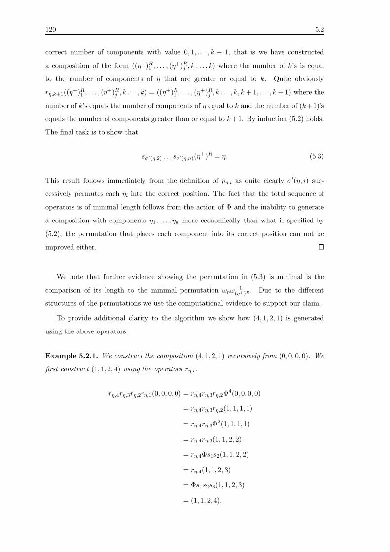
120 5.2
correct number of components with value 0, 1, . . . , k − 1, that is we have constructed
a composition of the form ((η+)R1 , . . . , (η+)Rj , k . . . , k) where the number of k’s is equal
to the number of components of η that are greater or equal to k. Quite obviously
rη,k+1((η+)R1 , . . . , (η
+)Rj , k . . . , k) = ((η+)R1 , . . . , (η+)Rj , k . . . , k, k + 1, . . . , k + 1) where the
number of k’s equals the number of components of η equal to k and the number of (k+1)’s
equals the number of components greater than or equal to k+1. By induction (5.2) holds.
The final task is to show that
sσ′(η,2) . . . sσ′(η,n)(η+)R = η. (5.3)
This result follows immediately from the definition of pη,i as quite clearly σ′(η, i) suc-
cessively permutes each ηi into the correct position. The fact that the total sequence of
operators is of minimal length follows from the action of Φ and the inability to generate
a composition with components η1, . . . , ηn more economically than what is specified by
(5.2), the permutation that places each component into its correct position can not be
improved either.
We note that further evidence showing the permutation in (5.3) is minimal is the
comparison of its length to the minimal permutation ωηω−1(η+)R
. Due to the different
structures of the permutations we use the computational evidence to support our claim.
To provide additional clarity to the algorithm we show how (4, 1, 2, 1) is generated
using the above operators.
Example 5.2.1. We construct the composition (4, 1, 2, 1) recursively from (0, 0, 0, 0). We
first construct (1, 1, 2, 4) using the operators rη,i.
rη,4rη,3rη,2rη,1(0, 0, 0, 0) = rη,4rη,3rη,2Φ4(0, 0, 0, 0)
= rη,4rη,3rη,2(1, 1, 1, 1)
= rη,4rη,3Φ2(1, 1, 1, 1)
= rη,4rη,3(1, 1, 2, 2)
= rη,4Φs1s2(1, 1, 2, 2)
= rη,4(1, 1, 2, 3)
= Φs1s2s3(1, 1, 2, 3)
= (1, 1, 2, 4).

5.3 121
We complete the generation by permuting each component into its correct position
sσ′(η,2)sσ′(η,3)sσ′(η,4)(1, 1, 2, 4) = sσ′(η,2)sσ′(η,3)s3s2(1, 1, 2, 4)
= sσ′(η,2)sσ′(η,3)(1, 2, 4, 1)
= sσ′(η,2)s2(1, 2, 4, 1)
= sσ′(η,2)(1, 4, 2, 1)
= s1(1, 4, 2, 1)
= (4, 1, 2, 1).
We now move onto the major goal of our study, the recursive generation of various
polynomial classes.
5.3 Recursively generating polynomials
There are many families of polynomials that can be recursively generated via switching
and raising type operators. Some examples are the nonsymmetric Macdonald polynomial
(Section 2.1.3), nonsymmetric interpolation Macdonald polyomials (Section 2.2.4), non-
symmetric Jack polynomials (Appendix C), nonsymmetric interpolation Jack polynomials
(Appendix D) and the generalised nonsymmetric Hermite and Laguerre polynomials (see
e.g. [23, Chap. 13]). In this section we show how the algorithm developed in Proposition
5.2.1 can be employed to recursively generate any of the polynomials in these families.
For simplicity in this section we use Fη(z) to denote any of the aforementioned families
of polynomials. We show how the recursive generation formulas work in the general setting
and then provide a specific example for the nonsymmetric Macdonald polynomials.
To most simply express the sequence of operators required to recursively generate a
composition according to Proposition 5.2.1 we use the numbers 1, . . . , n − 1 to represent
the allowable switching operators, 0 to represent the raising operator and denote the
required sequence by R(η). For Example 5.2.1 in the previous section we observe that
R((4, 1, 2, 1)) = 0, 0, 0, 0, 0, 0, 2, 1, 0, 3, 2, 1, 0, 2, 3, 2, 1.
Proposition 5.3.1. Define
RGj(Fη(j)(z), η(j), R(η)j) :=
Fsiη(j)(z), siη(j), i = R(η)j = 1, . . . , n − 1
FΦη(j)(z),Φη(j), i = R(η)j = 0,(5.4)

122 5.3
where η(j) represents the composition obtained after j transformations from (0, . . . , 0) to
η specified by R(η) and Fsiη(z) and FΦη(z) are obtained from Fη(z) using known formulas.
With initial input RG1(1, (0, . . . , 0),R(η)1) and each subsequent polynomial derived from
the previous by entering the newly obtained polynomial and composition along with the
next number in R(η) in RG the polynomial Fη(z) will be obtained after |R(η)| steps.
Proof. By Proposition 5.2.1 we know that the sequence specified by R(η) will recursively
generate the composition η from (0, . . . , 0). Consequently RGj will recursively generate
Fη(z) from F(0,...,0)(z).
We note that we keep track of the composition labelling the polynomial at each stage
due to requirements of the formulas transforming Fη(z) to Fsiη(z) and FΦη(z).
Example 5.3.1. To recursively generate a nonsymmetric Macdonald polynomial using the
methods in the previous proposition we begin by rewriting the formulas of Section 2.1.3 as
Esiη(z) =
t−1TiEη(z)−t−1
t(1−δ−1i,η (q,t))
Eη(z), ηi < ηi+1
Eη(z), ηi = ηi+1
(1−δi,η(q,t))2
(1−tδi,η(q,t))(1−t−1δi,η(q,t))
(TiEη(z)
t−11−δ−1
i,η (q,t)Eη(z)
), ηi > ηi+1,
EΦη(z) =t#i>1:ηi≤η1ΦqEη(z).
To generate the polynomial E(2,1)(z; q, t) from E(0,0)(z; q, t) = 1 using RG we first compute
R((2, 1)) using Proposition 5.2.1 to be R(2, 1) = 0, 0, 0, 1 we then proceed recursively
RG1(1, (0, 0), 0) = E(0,1)(z), (0, 1)
RG2(E(0,1)(z), (0, 1), 0) = E(1,1)(z), (1, 1)
RG3(E(1,1)(z), (1, 1), 0) = E(1,2)(z), (1, 2)
RG4(E(1,2)(z), (1, 2), 1) = E(2,1)(z), (2, 1).
In the cases where Fη(z) is homogeneous we can greatly reduce the number of operators
required to generate polynomials labelled by compositions with no zero components by
making use of the relationship
Fη+(kn)(z) = (z1 . . . zn)kFη(z), (5.5)

5.4 123
(c.f. (2.1.4)). This result allows us to omit the first n×minη zeros from R(η), forming
a new set R′(η), and begin our recursive process with
(z1 . . . zn)minη, (minη, . . . ,minη),R′(η)1
rather than 1, (0, . . . , 0),R(η)1.
Example 5.3.2. Using (5.5) we recursively generate E(2,1)(z; q, t) from E(1,1)(z; q, t).
With R′((2, 1)) = 0, 1 we obtain
RG1(z1z2, (1, 1), 0) = E(1,2)(z), (1, 2)
RG2(E(1,2)(z), (1, 2), 1) = E(2,1)(z), (2, 1).
5.4 Runtimes and Software
5.4.1 Algorithm runtimes
We now have two methods for recursively generating the nonsymmetric Macdonald and
nonsymmetric interpolation Macdonald polynomials; the Rodrigues formulas (Sections
2.1.4 and 2.2.5) and the algorithm specified by Proposition 5.3.1. We examine the efficiency
of our algorithm by comparing generation runtimes against the Rodrigues methods for
various polynomials.
To provide a thorough analysis we must select polynomials of varying degrees of com-
plexity. That is, varying the number of variables, the maximum degree and of these
polynomials selecting those requiring the least and most number of operators to generate.
Of the polynomials with n variables and maximum degree k those that take the least and
most number of operators to generate using the algorithm of Proposition 5.3.1 are labelled
by compositions (qn−r, (q+1)r) and (k, 0, . . . , 0), where k = qn+ r, and require k and nk
operators to generate, respectively. Similarly, using the Rodrigues methods, of the polyno-
mials with n variables and maximum degree k those that take the least and most number
of operators to generate are labelled by compositions ((q+1)r , qn−r)) and (0, . . . , 0, k) and
require nq + (n− (r − 1))r and n(k + 1)− 1 operators to generate, respectively. We note
that we have employed (5.5) into our algorithm and polynomials labelled by compositions
with no zero components will be generated more efficiently than what is specified above,
for example the nonsymmetric Macdonald polynomials labelled by η = (kn) would be
generated almost instantly.

124 5.4
Table 5.1 shows the runtimes of the generation of different nonsymmetric Macdonald
polynomials using the recursive generation algorithm of Proposition 5.3.1 and the Ro-
drigues formulas. The computer these runtimes were observed on was an iMac 2.4GHz
Intel core 2 duo processor in version 7.01.0 of Mathematica.
Eη(z) E∗η(z)
|η| η Recursive Generation Rodrigues Recursive Generation Rodrigues
4 (0, 4) 0.0308 6.6782 0.7792 205.972
(1, 3) 0.0064 1.1256 0.0759 11.4942
(2, 2) 0.0011 0.0648 0.0009 0.1281
(3, 1) 0.0177 0.6116 0.6081 5.0752
(4, 0) 0.0674 3.6920 12.3216 109.839
(0, 0, 4) 228.33 15.9176 4.54 4458.24
(1, 1, 2) 0.0014 2.6550 0.0010 11.1048
(2, 1, 1) 0.0105 1.0142 0.3108 3.3316
(4, 0, 0) 0.6337 92.8975 65.7861 2330.89
(1, 3, 0) 0.3171 66.1389 30.3733 3201.16
7 (0, 7) 0.2677 127.8250 34.4630 25888.1
(3, 4) 0.0019 0.5252 0.001648 7.2465
(4, 3) 0.0070 0.2074 0.1471 1.6495
(7, 0) 0.4744 54.3738 68.2642 9887.15
Table 5.1: Runtimes in seconds of Rodrigues formulas and recursive generation algorithm
It is the number and complexity of operators required to generate the polynomials using
the Rodrigues formulas that make them considerably more time consuming to use than
the algorithm we have constructed. However, one advantage of the Rodrigues formulas is
that it is much easier to implement into computer software. We also note that it is the
inhomogeniety of the interpolation polynomials that makes their construction time longer
than the nonsymmetric polynomials.
5.4.2 Mathematica notebook
We now provide the details of the Mathematica notebook containing the polynomials
and operators contained in this thesis. The Mathematica notebook, titled SpecialFunc-
tions.nb, can be found at www.ms.unimelb.edu.au/ ˜ wbaratta/index.html and

5.4 125
ran on Mathematica 7. The original purpose of the Mathematica notebook was to effi-
ciently generate nonsymmetric and nonsymmetric interpolation Macdonald polynomials
to develop an understanding of their known theory. Surpassing this motivation it has been
extensively used throughout the research period to assist with conjecture formulation and
testing. We now present a table containing the key functions defined in the Mathematica
notebook. The notations used in the table are consistent with those used throughout the
thesis.
Syntax Description
CompositionModulus[η] Computes |η|SwitchComposition[η, i] Computes siηRaiseComposition[η] Computes ΦηcI[η, I] Computes cI(η)
Dominance[η, λ] Determines whether η ≤ λ or λ ≤ ηPartialOrder[η, λ] Determines whether η λ or λ ηPartialOrder2[η, λ] Determines whether η ⊳ λ or λ ⊳ ηSuccessor[η, λ] Determines whether η ′ λ or λ ′ η
ArmLength[η, i, j] Computes aη(i, j)ArmCoLength[η, i, j] Computes a′η(i, j)
LegLength[η, i, j] Computes lη(i, j)LegCoLength[η, i] Computes l′η(i)
Md[η] Computes dη(q, t)MdDash[η] Computes d′η(q, t)
Me[η] Computes eη(q, t)MeDash[η] Computes e′η(q, t)
R[η] Computes the set R(η), specifying the sequence of operatorsrequired to generate η from (0, . . . , 0)
Table 5.2: Mathematica functions relating to compositions
Syntax Description
PermutationOnComposition[σ, η] Computes σ(η)DecompositionOnComposition[si1 , . . . , sil, η] Computes sil . . . si1ηSwitchingOperator[f, i, j] Computes sijf(. . . , zi, . . . , zj , . . .)PermutationOnPolynomial[σ, f ] Computes σf(z1, . . . , zn)ShortestPermutation[η] Computes ωη, the shortest
permutation such that ω−1η (η) = η+
RequiredPermutation[η, λ] Computes the permutation σ suchthat σ(η) = λ
Table 5.3: Mathematica functions relating to permutations

126 5.4
Syntax Description
Monomial[η] Computes zη
ElementarySymmetricFunction[r, n] Computes er(z) in n variablesCompleteSymmetricFunction[r, n] Computes hr(z) in n variablesSymmetricMonomialFunction[κ] Computes mκ(z)
Vandermonde[n] Computes ∆(z)VandermondeJ[J ] Computes ∆J(z)tVandermonde[n] Computes ∆t(z)tVandermondeJ[J ] Computes ∆J
t (z)
Schur[κ] Computes sκ(z)Zonal[κ] Computes Zκ(z)HallLittlewood[κ] Computes Pκ(z; t)
Table 5.4: Mathematica functions relating to miscellaneous polynomials
Syntax Description
SymJack[κ] Computes Pκ(z;α)NSJack[η] Computes Eη(z;α)IntJack[η] Computes E∗
η(z;α)
JEvalue[η] Computes ηα, where ηi := αηi − l′η(i)
EOpSymJack[f, n] Computes D2(α)fEOpNSJack[f, n, i] Computes ξifEOpIntJack[f, n, i] Computes Ξα
i f
JInnerProduct[f, g, n, k] Computes 〈f, g〉1/k for polynomials f, g of n variables
Table 5.5: Mathematica functions relating to Jack polynomials
Syntax Description
NSMac[η] Computes Eη(z; q, t)SymMac[κ] Computes Pκ(z; q, t)ASymMac[κ] Computes Sκ(z; q, t)
IntMac[η] Computes E∗η(z; q, t)
SymIntMac[κ] Computes P ∗κ (z; q, t)
ASymIntMac[κ] Computes S∗κ(z; q, t)
MEvalue[η] Computes η, where ηi := qηitl′η(i)
EOpSymMac[f, n] Computes D1n(q, t)f
EOpNSMac[f, i] Computes YifEOpIntMac[f, i] Computes Ξif
Ti[f, i] Computes Tif
TiInv[f, i] Computes T−1i f
Phiq[f, n] Computes ΦqfHi[f, i] Computes HifPhiqInt[f, n] Computes Φ∗
qf
MInnerProduct[f, g, n, k] Computes 〈f, g〉q,qk , for polynomials f, g of n variables
Table 5.6: Mathematica functions relating to Macdonald polynomials
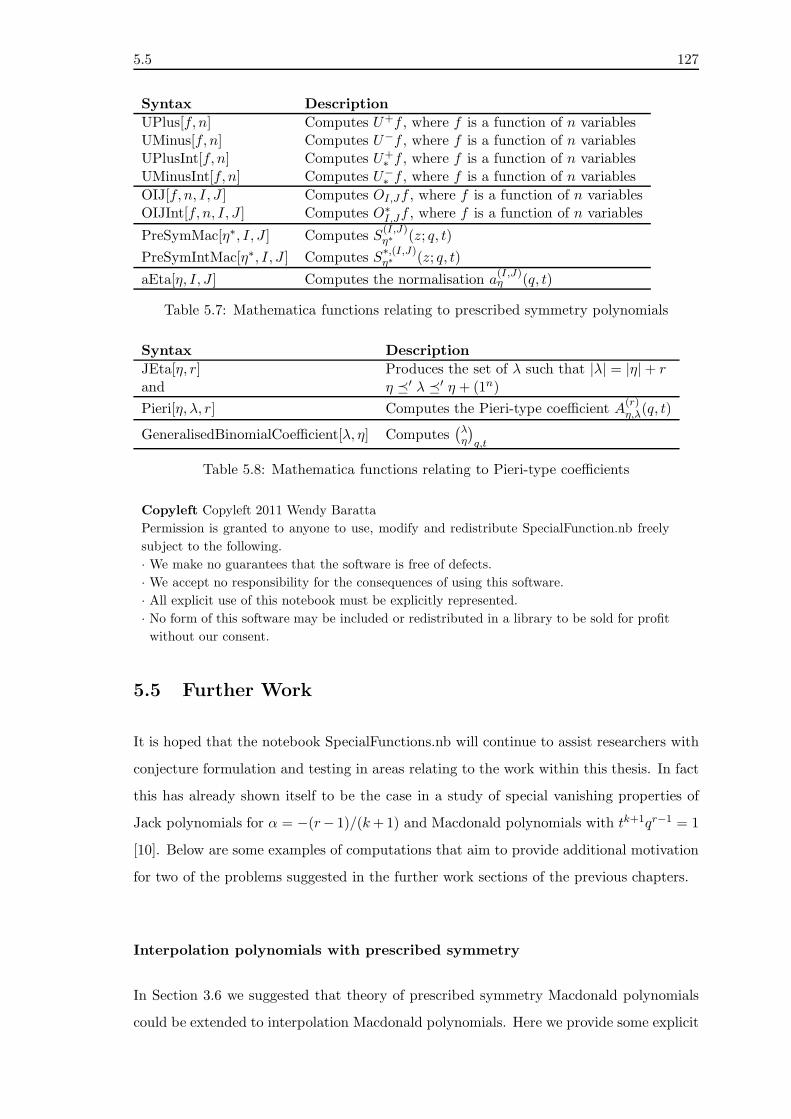
5.5 127
Syntax Description
UPlus[f, n] Computes U+f , where f is a function of n variablesUMinus[f, n] Computes U−f , where f is a function of n variablesUPlusInt[f, n] Computes U+
∗ f , where f is a function of n variablesUMinusInt[f, n] Computes U−
∗ f , where f is a function of n variables
OIJ[f, n, I, J ] Computes OI,Jf , where f is a function of n variablesOIJInt[f, n, I, J ] Computes O∗
I,Jf , where f is a function of n variables
PreSymMac[η∗, I, J ] Computes S(I,J)η∗ (z; q, t)
PreSymIntMac[η∗, I, J ] Computes S∗,(I,J)η∗ (z; q, t)
aEta[η, I, J ] Computes the normalisation a(I,J)η (q, t)
Table 5.7: Mathematica functions relating to prescribed symmetry polynomials
Syntax Description
JEta[η, r] Produces the set of λ such that |λ| = |η|+ rand η ′ λ ′ η + (1n)
Pieri[η, λ, r] Computes the Pieri-type coefficient A(r)η,λ(q, t)
GeneralisedBinomialCoefficient[λ, η] Computes(λη
)q,t
Table 5.8: Mathematica functions relating to Pieri-type coefficients
Copyleft Copyleft 2011 Wendy Baratta
Permission is granted to anyone to use, modify and redistribute SpecialFunction.nb freely
subject to the following.
· We make no guarantees that the software is free of defects.
· We accept no responsibility for the consequences of using this software.
· All explicit use of this notebook must be explicitly represented.
· No form of this software may be included or redistributed in a library to be sold for profit
· without our consent.
5.5 Further Work
It is hoped that the notebook SpecialFunctions.nb will continue to assist researchers with
conjecture formulation and testing in areas relating to the work within this thesis. In fact
this has already shown itself to be the case in a study of special vanishing properties of
Jack polynomials for α = −(r− 1)/(k+1) and Macdonald polynomials with tk+1qr−1 = 1
[10]. Below are some examples of computations that aim to provide additional motivation
for two of the problems suggested in the further work sections of the previous chapters.
Interpolation polynomials with prescribed symmetry
In Section 3.6 we suggested that theory of prescribed symmetry Macdonald polynomials
could be extended to interpolation Macdonald polynomials. Here we provide some explicit

128 5.5
computations that may assist with the identification of the relationship between the anti-
symmetric interpolation polynomial S∗κ+δ(z) and the symmetric interpolation polynomial
P ∗κ (z).
space
In[1] SymIntMac[ 1, 0]
Out[1]t (x1 + x2)− t− 1
t
In[2] ASymIntMac[ 2, 0]
Out[2](x1 − tx2) (t (x1 + x2)− qt− 1)
t
space
In[1] SymIntMac[ 1, 1]
Out[1](tx1 − 1) (tx2 − 1)
t2
In[2] ASymIntMac[ 2, 1]
Out[2](x1 − tx2) (tx1 − 1) (tx2 − 1)
t2
space
In[1] SymIntMac[ 1, 0, 0]
Out[1]t2 (x1 + x2 + x3)− t2 − t− 1
t2
In[2] ASymIntMac[ 3, 1, 0]
Out[2](x1 − tx2) (x1 − tx3) (x2 − tx3)
(t2 (x1 + x2 + x3)− qt(qt+ 1)− 1
)
t2
space
These computations show a clear relationship between S∗κ+δ(z) and P ∗
κ (z), highlighting
that the difficulty in identifying the relationship lies in the transformations of the param-
eters. It also appears that the t-Vandermonde product that relates the polynomials is not
of standard form.
Pieri-type formulas for nonsymmetric Macdonald polynomials
It is stated in Section 4.5 that trial computations show that the Pieri-type formulas for the
nonsymmetric Macdonald polynomials can generally be expressed as products. In Section
4.5 we provided an explicit formula for the r = 1 case and left the remaining cases as an
open problem. Here we present explicit formulas for the Pieri-type coefficients for the case
r = 2.

129
space
In[1] Pieri[ 1, 0, 1, 0, 2, 0, 2, 0, 2] ee In[2] Pieri[ 1, 0, 1, 0, 2, 1, 1, 0, 2]
Out[1] 1 Out[2]q − 1
qt− 1space
In[3] Pieri[ 1, 0, 1, 0, 1, 1, 2, 0, 2] ee In[4] Pieri[ 1, 0, 1, 0, 2, 0, 1, 1, 2]
Out[3]t(q − 1)
(qt3 − 1
)
(qt2 − 1)2Out[4]
t(q − 1)(qt3 − 1
)
(qt2 − 1)2
space
In[5] Pieri[ 1, 0, 1, 0, 1, 1, 1, 1, 2] ee In[6] Pieri[ 1, 0, 1, 0, 1, 2, 0, 1, 2]
Out[5](q − 1)(qt− 1)
(qt4 − 1
)
(qt2 − 1)3Out[6]
q2t2(q − 1)(t− 1)4
(qt− 1)3 (qt2 − 1)2
space
In[7] Pieri[ 1, 0, 1, 0, 1, 2, 1, 0, 2] ee In[8] Pieri[ 1, 0, 1, 0, 2, 1, 0, 1, 2]
Out[7] −qt(q − 1)(t − 1)2
(qt− 1)2 (qt2 − 1)Out[8] −
qt(q − 1)(t− 1)2
(qt− 1)2 (qt2 − 1)space
In[9] Pieri[ 1, 0, 1, 0, 0, 2, 2, 0, 2] t In[10] Pieri[ 1, 0, 1, 0, 2, 0, 0, 2, 2]
Out[9]qt2(q − 1)(t − 1)
(qt− 1)(qt+ 1) (qt2 − 1)Out[10]
qt2(q − 1)(t− 1)
(qt− 1)(qt+ 1) (qt2 − 1)space
In[11] Pieri[ 1, 0, 1, 0, 1, 0, 2, 1, 2]
Out[11](q − 1)t2
(q(t(q((q − 2)qt5 + (3q − 1)t4 + (2− 3q)t3 − 2t+ 1
)+ 3(t− 1)
)+ 2)− 1)
(qt− 1) (qt2 − 1)2 (q2t3 − 1)space
In the above formulas for the Pieri-type coefficients A(2)(1,0,1,0),λ(q, t) a simple product struc-
ture in q and t, with roots in t being simple fractional powers of q for example, is exhibited
in all cases except λ = (1, 0, 2, 1). Additional trial computations suggest that it is always
the successor of the form ΦΦη that cannot be expressed as a simple product.

130

Bibliography
[1] G. E. Andrews. Problems and prospects for basic hypergeometric functions. In Theory
and application of special functions, pages 191–224. Mathematics Research Center,
University of Wisconsin, Publication Number 35. Academic Press, New York, 1975.
[2] T. H. Baker, C. F. Dunkl, and P. J. Forrester. Polynomial eigenfunctions of the
Calogero-Sutherland-Moser models with exchange terms. CRM Series Mathematical
Physics, pages 37–51, 2000.
[3] T. H. Baker and P. J. Forrester. Generalized weight functions and the Macdonald
polynomials. q-alg/9603005, 1996.
[4] T. H. Baker and P. J. Forrester. The Calogero-Sutherland model and polynomials
with prescribed symmetry. Nuclear Physics. B, 492(3):682–716, 1997.
[5] T. H. Baker and P. J. Forrester. A q-analogue of the type A Dunkl operator and
integral kernel. International Mathematics Research Notices, (14):667–686, 1997.
[6] T. H. Baker and P. J. Forrester. Generalizations of the q-Morris constant term identity.
Journal of Combinatorial Theory. Series A, 81(1):69–87, 1998.
[7] T. H. Baker and P. J. Forrester. Isomorphisms of type A affine Hecke algebras and
multivariable orthogonal polynomials. Pacific Journal of Mathematics, 194(1):19–41,
2000.
[8] T. H. Baker and P. J. Forrester. Multivariable Al-Salam & Carlitz polynomials asso-
ciated with the type A q-Dunkl kernel. Mathematische Nachrichten, 212:5–35, 2000.
[9] W. Baratta. Pieri-type formulas for nonsymmetric Macdonald polynomials. Interna-
tional Mathematics Research Notices, (15):2829–2854, 2009.
[10] W. Baratta and P. J. Forrester. Jack polynomials fractional quantum Hall states and
their generalizations. 2010. arXiv:1007.2692.
131

132
[11] D. M. Bressoud and I. P. Goulden. Constant term identities extending the q-Dyson
theorem. Transactions of the American Mathematical Society, 291(1):203–228, 1985.
[12] I. Cherednik. A unification of Knizhnik-Zamolodchikov and Dunkl operators via affine
Hecke algebras. Inventiones Mathematicae, 106(2):411–431, 1991.
[13] I. Cherednik. Integration of quantum many-body problems by affine Knizhnik-
Zamolodchikov equations. Advances in Mathematics, 106(1):65–95, 1994.
[14] I. Cherednik. Double affine Hecke algebras and Macdonald’s conjectures. Annals of
Mathematics. Second Series, 141(1):191–216, 1995.
[15] I. Cherednik. Nonsymmetric Macdonald polynomials. International Mathematics
Research Notices, (10):483–515, 1995.
[16] J. Demmel and P. Koev. Accurate and efficient evaluation of Schur and Jack functions.
Mathematics of Computation, 75(253):223–239 (electronic), 2006.
[17] I. Dumitriu, A. Edelman, and G. Shuman. MOPS: multivariate orthogonal polyno-
mials (symbolically). Journal of Symbolic Computation, 42(6):587–620, 2007.
[18] C. F. Dunkl. Orthogonal polynomials of types A and B and related Calogero models.
Communications in Mathematical Physics, 197(2):451–487, 1998.
[19] F. J. Dyson. Statistical theory of energy levels of complex symbols. International
Journal of Mathematical Physics, 3:140–156, 1962.
[20] R. H. Farrell. Calculation of complex zonal polynomials. In Multivariate analysis, V,
pages 301–320. North-Holland, Amsterdam, 1980.
[21] B. Feigin, M. Jimbo, T. Miwa, and E. Mukhin. Symmetric polynomials vanishing
on the shifted diagonals and Macdonald polynomials. International Mathematics
Research Notices, (18):1015–1034, 2003.
[22] P. J. Forrester. Addendum to Selberg correlation integrals and the 1/r2 quantum
many body system. Nuclear Physics, 416:377–385, 1994.
[23] P. J. Forrester. Log-gases and random matrices. Princeton University Press, Prince-
ton, NJ, 2010.
[24] P. J. Forrester and D. S. McAnally. Pieri-type formulas for the non-symmetric Jack
polynomials. Commentarii Mathematici Helvetici, 79(1):1–24, 2004.

133
[25] P. J. Forrester, D. S. McAnally, and Y. Nikoyalevsky. On the evaluation formula for
Jack polynomials with prescribed symmetry. Journal of Physics. A, 34(41):8407–8424,
2001.
[26] P. J. Forrester and E. M. Rains. Interpretations of some parameter dependent gen-
eralizations of classical matrix ensembles. Probability Theory and Related Fields,
131(1):1–61, 2005.
[27] P. J. Forrester and S. O. Warnaar. The importance of the Selberg integral. American
Mathematical Society. Bulletin. New Series, 45(4):489–534, 2008.
[28] I. M. Gessel, L. Lv, G. Xin, and Y. Zhou. A proof of Askey’s conjectured q-analogue
of Selberg’s integral and a conjecture of Morris. SIAM Journal on Mathematical
Analysis, 19(4):969–986, 1988.
[29] J. A. Green. The characters of the finite general linear groups. Transactions of the
American Mathematical Society, 80:402–447, 1955.
[30] L. Habsieger. Une q-integrale de Selberg-Askey. SIAM Journal on Mathematical
Analysis, (19):1475–1489, 1988.
[31] M. Haiman. Hilbert schemes, polygraphs and the Macdonald positivity conjecture.
Journal of the American Mathematical Society, 14(4):941–1006 (electronic), 2001.
[32] F. D. M. Haldane. Exact jastrow-gutzwiller resonating-valence-bond ground state of
the spin-1/2 antiferromagnetic heisenberg chain with 1/r2 exchange. Physical Review
Letters, 60:635–638, 1988.
[33] P. Hall. The algebra of partitions. Proceedings of the 4th Canadian Mathematics
Congress, Banff, 1959.
[34] S. Hamada. Proof of Baker-Forrester’s constant term conjecture for the cases N1 =
2, 3. Kyushu Journal of Mathematics, 56(2):243–266, 2002.
[35] L. K. Hua. Harmonic analysis of functions of several complex variables in the classical
domains. Translated from the Russian by Leo Ebner and Adam Koranyi. American
Mathematical Society, Providence, R.I., 1963.
[36] H. Jack. A class of symmetric polynomials with a parameter. Proceedings of the Royal
Society of Edinburgh. Section A. Mathematics, 69:1–18, 1970/1971.

134
[37] H. Jack. A surface integral and symmetric functions. Proceedings of the Royal Society
of Edinburgh. Section A. Mathematics, 69(part 4):347–364, 1972.
[38] C. Jacobi. De functionibus alternantibus earemque divisione per productum e differ-
entiis elementorum conluatum. Journal fur die Reine und Angewandte Mathematik,
22:360–371, 1841.
[39] A. T. James. Zonal polynomials of the real positive definite symmetric matrices.
Annals of Mathematics. Second Series, 74:456–469, 1961.
[40] K. W. J. Kadell. A proof of Askey’s conjectured q-analogue of Selberg’s integral and a
conjecture of Morris. SIAM Journal on Mathematical Analysis, 19(4):969–986, 1988.
[41] K. W. J. Kadell. A proof of some analogues of Selberg’s integral for k = 1. SIAM
Journal on Mathematical Analysis, 19(4):944–968, 1988.
[42] Y. Kato and T. Yamamoto. Jack polynomials with prescribed symmetry and hole
propagator of spin Calogero-Sutherland model. Journal of Physics. A, 31(46):9171–
9184, 1998.
[43] A. N. Kirillov and A. Alexander. Lectures on affine Hecke algebras and Macdonald’s
conjectures. American Mathematical Society. Bulletin, 34(3):251–292, 1997.
[44] F. Knop. Symmetric and non-symmetric quantum Capelli polynomials. Commentarii
Mathematici Helvetici, 72(1):84–100, 1997.
[45] F. Knop and S. Sahi. Difference equations and symmetric polynomials defined by
their zeros. International Mathematics Research Notices, (10):473–486, 1996.
[46] T. H. Koornwinder. q-special functions, an overview, 2005. arXiv:math/0511148v1.
[47] V. B. Kuznetsov and S. Sahi, editors. Jack, Hall-Littlewood and Macdonald polyno-
mials, volume 417 of Contemporary Mathematics, Providence, RI, 2006. American
Mathematical Society.
[48] L. Lapointe and L. Vinet. Rodrigues formulas for the Macdonald polynomials. Ad-
vances in Mathematics, 130(2):261–279, 1997.
[49] A. Lascoux. Schurbert and Macdonald polynomials, a parallel.
http://phalanstere.univ-mlv.fr/al/.
[50] A. Lascoux and M. P. I Schutzenberger. Polynomes de Schubert. Comptes Rendus des
Seances de l’Academie des Sciences. Serie I. Mathematique, 294(13):447–450, 1982.

135
[51] D. E. Littlewood. On certain symmetric functions. Proceedings of the London Math-
ematical Society. Third Series, 11:485–498, 1961.
[52] I. G. Macdonald. Spherical functions on a group of p-adic type. Akademiya Nauk
SSSR i Moskovskoe Matematicheskoe Obshchestvo. Uspekhi Matematicheskikh Nauk,
28(5 (173)):155–224, 1973.
[53] I. G. Macdonald. A new class of symmetric functions. Actes du 20e Seminare Lotharig-
nien, 372/S-20:131–171, 1988.
[54] I. G. Macdonald. Symmetric functions and Hall polynomials. The Clarendon Press
Oxford University Press, New York, second edition, 1995.
[55] I. G. Macdonald. Affine Hecke algebras and orthogonal polynomials, volume 157 of
Cambridge Tracts in Mathematics. Cambridge University Press, Cambridge, 2003.
[56] D. Marshall. Macdonald polynomials. Masters thesis, The University of Melbourne,
1999.
[57] D. Marshall. Symmetric and nonsymmetric Macdonald polynomials. Annals of Com-
binatorics, 3(2-4):385–415, 1999.
[58] D. Marshall. The product of a nonsymmetric Jack polynomial with a linear func-
tion. Proceedings of the American Mathematical Society, 131(6):1817–1827 (elec-
tronic), 2003.
[59] A. Mathas. Iwahori-Hecke algebras and Schur algebras of the symmetric group, vol-
ume 15 of University Lecture Series. American Mathematical Society, Providence,
RI, 1999.
[60] K. Mimachi and M. Noumi. A reproducing kernel for nonsymmetric Macdonald
polynomials. Duke Mathematical Journal, 91(3):621–634, 1998.
[61] W. G. Morris. Constant term identities for finite affine root systems, PhD thesis.
University of Wisconsin, Madison, 1982.
[62] R. J. Muirhead. Aspects of multivariate statistical theory. John Wiley & Sons Inc.,
New York, 1982. Wiley Series in Probability and Mathematical Statistics.
[63] A. Nishino, H. Ujino, and M. Wadati. An algebraic approach to the non-symmetric
Macdonald polynomial. Nuclear Physics. B, 558(3):589–603, 1999.

136
[64] A. Nishino, H. Ujino, and M. Wadati. Rodrigues formula for the nonsymmetric
Macdonald polynomial. Journal of the Physical Society of Japan, 68(3):701–704,
1999.
[65] A. Nishino, H. Ujino, and M. Wadati. Rodrigues formula for the nonsymmetric mul-
tivariable Laguerre polynomial. Journal of the Physical Society of Japan, 68(3):797–
802, 1999.
[66] A. Okounkov. Binomial formula for Macdonald polynomials and applications. Math-
ematical Research Letters, 4(4):533–553, 1997.
[67] S. Sahi. Interpolation, integrality, and a generalization of Macdonald’s polynomials.
International Mathematics Research Notices, (10):457–471, 1996.
[68] S. Sahi. A new scalar product for nonsymmetric Jack polynomials. International
Mathematics Research Notices, (20):997–1004, 1996.
[69] S. Sahi. The binomial formula for nonsymmetric Macdonald polynomials. Duke
Mathematical Journal, 94(3):465–477, 1998.
[70] I. Schur. uber ein Klass von Matrizen die sich einer gegebenen Matrix zuordnen
lassen. Dissertation, Berlin, (1):1–72, 1901.
[71] W. Schutzer. On some combinatorial aspects of representation theory. PhD thesis,
the University of New Brunswick, New Jersey, 2004.
[72] B. S. Shastry. Exact solution of an s = 1/2 Heisenberg antiferromagnetic chain with
long-range interactions. Physical Review Letters, 60:639–642, 1988.
[73] R. P. Stanley. Enumerative combinatorics. Vol. 1. Cambridge University Press, New
York/-Cambridge, 1997.
[74] A. Takamura and K. Takano. Braid structure and raising-lowering operator formalism
in Sutherland model. Journal of Physics. A, 31(25):L473–L480, 1998.
[75] A. Takemura. Zonal polynomials. Institute of Mathematical Statistics Lecture
Notes—Monograph Series, 4. Institute of Mathematical Statistics, Hayward, CA,
1984.
[76] H. Ujino and M. Wadati. Rodrigues formula for the nonsymmetric multivariable
Hermite polynomial. Journal of the Physical Society of Japan, 68(2):391–395, 1999.

137
[77] J. van Diejen and E. Emsiz. Pieri formulas for macdonald’s spherical functions and
polynomials. Mathematische Zeitschrift, pages 1–12, 2010. 10.1007/s00209-010-0727-
0.
[78] D. Zeilberger. A Stembridge-Stanton style elementary proof of the Habsieger-Kadell
q-Morris identity. Discrete Mathematics, 79(3):313–322, 1990.

138

Appendix A
Some basic q-functions
The q-factorial, q-binomial coefficient, q-Pochhammer symbol and q-gamma function, de-
noted [k]q!,(nk
)q, (a; q)k and Γq(z) respectively are given by
[k]q! := 1(1 + q)(1 + q + q2) . . . (1 + q + . . . + qk−1), (A.1)
(n
k
)
q
:=(q; q)n
(q; q)k(q; q)n−k, (A.2)
(a; q)k :=
∏k−1j=0(1− aqj), k > 0
∏∞j=0(1− aqj), k = ∞,
(A.3)
Γq(z) :=(q; q)∞(qz; q)∞
(1− q)1−z, (A.4)
each reducing to their classical counterparts when q → 1. Note that (a; q)∞ requires
|q| → 1 to be convergent. Like their classical counterparts there are alternative ways to
express the q-factorial and q-binomial coefficient. We have [46]
[k]q! =(q; q)k(1− q)k
= Γq(k + 1),
where the first equality follows from the identity
(1− qk) = (1− q)(1 + . . . + qk−1) (A.5)
139

140
and the second from (A.4), and we also have
(n
k
)
q
=[n]q!
[k]q![n− k]q!.
The q-gamma function satisfies the recurrence relation
Γq(z + 1) =1− qz
1− qΓq(z)
thus generalising the recurrence relation Γ(z + 1) = zΓ(z) of its classical counterpart.

Appendix B
Symmetric polynomials
B.1 Triangular structure
Class Notation and structure
Schur polynomials; sκ(z) = mκ(z) +∑
µ<κ
Kκµmµ(z)
zonal polynomials; Zκ(z) = mκ(z) +∑
µ<κ
K ′κµmµ(z)
Hall-Littlewood polynomials; Pκ(z; t) = mκ(z) +∑
µ<κ
Kκµ(t)mµ(z)
Symmetric Jack polynomials; Pκ(z;α) = mκ(z) +∑
µ<κ
Kκµ(α)mµ(z)
Symmetric Macdonald polynomials; Pκ(z; q, t) = mκ(z) +∑
µ<κ
Kκµ(q, t)mµ(z)
Class Coefficients
Schur polynomials; Kκµ ∈ Z
zonal polynomials; K ′κµ ∈ Q
Hall-Littlewood polynomials; Kκµ(t) ∈ Q(t)
Symmetric Jack polynomials; Kκµ(α) ∈ Q(α)
Symmetric Macdonald polynomials; Kκµ(q, t) ∈ Q(q, t)
141

142
B.2 Orthogonality
Class Alternative inner product
Schur polynomials; 〈pκ(z), pµ(z)〉1 = δκµcκ
zonal polynomials; 〈pκ(z), pµ(z)〉2 = δκµcκ2n
Hall-Littlewood polynomials; 〈pκ(z), pµ(z)〉q = δκµcκ∏n
i=1(1− tκi−1)
Symmetric Jack polynomials; 〈pκ(z), pµ(z)〉α = δκµcκαn
Symmetric Macdonald polynomials; 〈pκ(z), pµ(z)〉q,t = δκµcκ∏n
i=1
1− qκi
1− tκi
Class Explicit formula for the inner product
Schur polynomials; CT(sκ(z)sµ(z−1)W (z; 1))
Symmetric Jack polynomials; CT(Pκ(z;α)Pµ(z−1;α)W (z;α))
Symmetric Macdonald polynomials; CT(Pκ(z; q, t)Pµ(z−1; q−1, t−1)W (z; q, t))
Class Weight function
Schur polynomials; W (z; 1) :=∏
i<j
|zi − zj |2
Symmetric Jack polynomials; W (z;α) :=∏
i<j
|zi − zj |2/α
Symmetric Macdonald polynomials; W (z; q, t) :=∏
i<j
(zi/zj ; q)∞(qzi/zj ; q)∞(tzi/zj ; q)∞(qtzi/zj ; q)∞
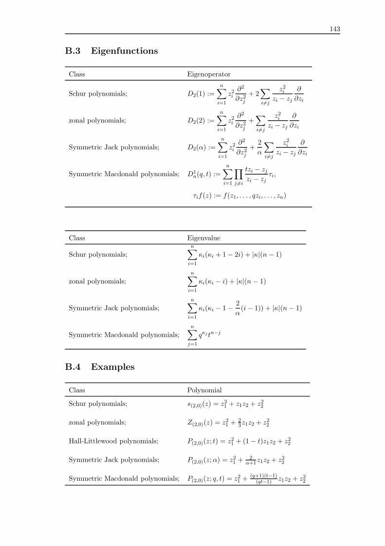
143
B.3 Eigenfunctions
Class Eigenoperator
Schur polynomials; D2(1) :=
n∑
i=1
z2i∂2
∂z2j+ 2
∑
i 6=j
z2izi − zj
∂
∂zi
zonal polynomials; D2(2) :=
n∑
i=1
z2i∂2
∂z2j+∑
i 6=j
z2izi − zj
∂
∂zi
Symmetric Jack polynomials; D2(α) :=
n∑
i=1
z2i∂2
∂z2j+
2
α
∑
i 6=j
z2izi − zj
∂
∂zi
Symmetric Macdonald polynomials; D1n(q, t) :=
n∑
i=1
∏
j 6=i
tzi − zjzi − zj
τi,
τif(z) := f(z1, . . . , qzi, . . . , zn)
Class Eigenvalue
Schur polynomials;
n∑
i=1
κi(κi + 1− 2i) + |κ|(n − 1)
zonal polynomials;
n∑
i=1
κi(κi − i) + |κ|(n − 1)
Symmetric Jack polynomials;
n∑
i=1
κi(κi − 1−2
α(i− 1)) + |κ|(n − 1)
Symmetric Macdonald polynomials;
n∑
j=1
qκj tn−j
B.4 Examples
Class Polynomial
Schur polynomials; s(2,0)(z) = z21 + z1z2 + z22
zonal polynomials; Z(2,0)(z) = z21 +23z1z2 + z22
Hall-Littlewood polynomials; P(2,0)(z; t) = z21 + (1− t)z1z2 + z22
Symmetric Jack polynomials; P(2,0)(z;α) = z21 +2
α+1z1z2 + z22
Symmetric Macdonald polynomials; P(2,0)(z; q, t) = z21 +(q+1)(t−1)
(qt−1) z1z2 + z22
asd

144
Remark: The details of the triangular structure, the defining properties of the inner
product and the explicit formulas for the Schur and Hall-Littlewood polynomials can
be found in [54]. The alternative inner product formulas for the symmetric Jack and
symmetric Macdonald can be found in [23, 57], respectively. The explicit formula for the
inner product of the Schur polynomials is obtained by taking α→ 1 in the Jack formula.
The details of the eigenoperator and eigenvalue for the Jack and zonal polynomials is in
[62], and once again taking the limit α → 1 to obtain the Schur details from the Jack.
The eigenoperator and eigenvalue of the Macdonald polynomial is found in [57].

Appendix C
Nonsymmetric Jack polynomials
C.1 Special function properties
Notation and structure; Eη(z;α) = zη +∑
λ<η
Kηλ(α)zλ,
Coefficients; Kηλ(α) ∈ Q(α)
Inner product; 〈f(z), g(z)〉α := CT(f(z)g(z−1)
∏
i<j
|zi − zj|2/α)
Eigenoperator; ξi := αzi∂
∂xi+∑
i<j
zizi − zj
(1− sij)
+∑
j<i
zjzi − zj
(1− sij) + 1− i
Eigenvalue; ηαi := αηi − l′η(i)
Switching operator; si
Raising operator; Φα := znsn−1 . . . s1
C.2 Recursive generation formulas
Esiη(z;α) =
siEη(z;α) −1
ηαi −ηαi+1Eη(z;α), ηi < ηi+1
Eη(z;α), ηi = ηi+1(1− 1
(ηαi −ηαi+1)2
)−1(siEη(z;α) −
1ηαi −ηαi+1
Eη(z;α)), ηi > ηi+1
EΦη(z) =ΦαEη(z)
145

146
C.3 Examples
η Eη(z;α) η Eη(z;α)
(0, 0, 0) 1 (0, 1, 1) z2z3
(0, 0, 1) z3 (1, 0, 1) z3(z1 +1
α+2z2)
(0, 1, 0) z2 +1
α+2z3 (0, 0, 2) z3(z3 +1
α+1 (z1 + z2))
(1, 0, 0) z1 +1
α+1 (z2 + z3)
Remark: The details within this appendix can be found in [23, Chap. 12].

Appendix D
Nonsymmetric Interpolation Jack
polynomials
D.1 Special function properties
Notation and structure; E∗η(z;α) = zη +
∑
λ⊳η
Kηλ(α)zλ,
Coefficients; Kηλ(α) ∈ Q(α)
Eigenoperator; Ξαi := zi − σi . . . σn−1
(zn −
n− 1
α
)∆(n)σ1 . . . σi−1
Eigenvalue; ηα,∗i := ηi −1
αl′η(i)
Switching operator; σi := si +1
α
1− sizi − zi+1
, i = 1, . . . , n− 1
Raising operator; Φ∗α :=
(zn +
n− 1
α
)∆(n),
∆(n)f(z) := f(zn − 1, z1, . . . , zn−1)
D.2 Recursive generation formulas
E∗siη(z;α) =
σiE∗η(z;α) −
1ηαi −ηαi+1
E∗η(z;α), ηi < ηi+1
E∗η(z;α) , ηi = ηi+1(1− 1
(ηαi −ηαi+1)2
)−1(σiE
∗η(z;α) −
1ηαi −ηαi+1
E∗η(z;α)
), ηi > ηi+1
E∗Φη(z) =Φ∗
αE∗η(z)
147

148
D.3 Examples
η E∗η(z;α) η E∗
η(z;α)
(0, 0, 0) 1 (0, 1, 1) z2z3 +2α(z2 + z3) +
4α2
(0, 0, 1) z3 +2α (1, 0, 1) z3(z1 +
1α+2z2) +
2αz1 +
2α(α+2)z2
(0, 1, 0) z2 +1
α+2z3 +4+α
α(α+2) + 4+αα(α+2)z3 +
2(4+α)α2(α+2)
(1, 0, 0) z1 +1
α+1 (z2 + z3) +3
α(α+1) (0, 0, 2) z3(z3 +1
α+1(z1 + z2)) +2
α(α+1) (z1 + z2)
+5+α−α2
α(α+1) z3 +2(3−α−α2)α2(α+1)
Remark: The details within this appendix can be found in [23, Chap. 12].

Minerva Access is the Institutional Repository of The University of Melbourne
Author/s:
BARATTA, WENDY
Title:
Special function aspects of Macdonald polynomial theory
Date:
2011
Citation:
Baratta, W. (2011). Special function aspects of Macdonald polynomial theory. PhD thesis,
Science, Department of Mathematics and Statistics, The University of Melbourne.
Persistent Link:
http://hdl.handle.net/11343/35978
File Description:
Special function aspects of Macdonald polynomial theory
Terms and Conditions:
Terms and Conditions: Copyright in works deposited in Minerva Access is retained by the
copyright owner. The work may not be altered without permission from the copyright owner.
Readers may only download, print and save electronic copies of whole works for their own
personal non-commercial use. Any use that exceeds these limits requires permission from
the copyright owner. Attribution is essential when quoting or paraphrasing from these works.

![Notes on Polynomial Functors - UAB Barcelonakock/cat/polynomial.pdf · 2018. 1. 11. · • Polynomial functors and polynomial monads [39] with Gambino • Polynomial functors and](https://img.pdfslide.net/doc/110x75/60faf8a63b5d714a860ca184/notes-on-polynomial-functors-uab-barcelona-kockcat-2018-1-11-a-polynomial.jpg)

![arXiv:1402.2203v3 [math.QA] 9 Sep 2016 · Macdonald polynomial in the untwisted and non-simply-laced cases, ... tensor products of column-shape KR crystals, for all untwisted a ne](https://img.pdfslide.net/doc/110x75/5b5cc03a7f8b9a9c398cc765/arxiv14022203v3-mathqa-9-sep-2016-macdonald-polynomial-in-the-untwisted.jpg)