SPECIAL ISSUE PAPER 1 Midcourse guidance law …web.mst.edu/~autosys/papers/002.pdfMidcourse guidance law with neural networks D Han, S N Balakrishnan , and E J Ohlmeyer† Department

Midcourse guidance law with neural networksD Han, S N Balakrishnan�, and E J Ohlmeyer†

Department of Mechanical and Aerospace Engineering, University of Missouri-Rolla, Rolla, Missouri, USA

The manuscript was received on 16 February 2004 and was accepted after revision for publication on 7 July 2004.

DOI: 10.1243/

Abstract: A dual neural network ‘adaptive critic approach’ is used in this study to generatemidcourse guidance commands for a missile to reach a predicted impact point while maxi-mizing its final velocity. The adaptive critic approach is based on approximate dynamic pro-gramming. The first network, called a ‘critic’, network, outputs the Lagrangian multipliersarising in an optimal control formulation while the second network, called an ‘action’ network,outputs the optimal guidance/control. While a typical adaptive critic structure consists of asingle critic and a single controller, the midcourse guidance problem needs indexing in termsof the independent variable and therefore there is a cascade of critics and controllers each setfor a different index. Every controller learns from the critic at the previous stage. Though thenetworks are trained off-line, the resulting control is in a feedback form. A midcourse guidanceproblem is the first testbed for this approach where the input is vector-valued. The numericalresults for a number of scenarios show that the network performance is excellent. Corroborationfor optimality is provided by comparisons of the numerical solutions using a shooting methodfor a number of scenarios. Numerical results demonstrate some attractive features of the adap-tive critic approach and show that this formulation works very well in guiding the missile toits final conditions from an envelope of initial conditions. This application also demonstratesthe use of adaptive critics as a tool to solve a class of ‘free final time’ problems in optimalcontrol, which are usually very difficult.

Keywords: missile, neural networks, optimal control

1 INTRODUCTION

Midcourse guidance considered in this study dealswith scenarios wherein a surface launched missileseeks to intercept an airborne target. In an optimalsetting, the resulting trajectory seeks to maximizethe pursuer velocity at the time of intercept. Twotypes of guidance law have been popular in themidcourse guidance literature; they are the explicitguidance [1] and the optimal curvature or kappaguidance [2–5]. A linearized form of kappa guidanceis proposed by Serakos and Lin [5] in which acoordinate transformation is used. All of theseguidance law are optimality based and use some

sort of approximations to the non-linear equationsof motion. The optimal neural guidance laws devel-oped in this study, however, allow the use of thenon-linear equations directly without the need forany approximations.

It is well known that the dynamic programmingformulation offers the most comprehensive solu-tion to non-linear optimal control; however, a hugeamount of computational and storage requirementsare needed to solve the associated Hamilton–Jacobi–Bellman (HJB) equation [6] (also known asthe Bellman equation). Werbos [7] proposed ameans to get around this numerical complexity byusing ‘approximate dynamic programming’ (ADP)formulations. His methods approximate the originalproblem with a discrete formulation. The solutionto the ADP formulation is obtained through thetwo neural network adaptive critic approach. Inone version of the adaptive critic approach, calleddual heuristic programming (DHP), one network,called the action network, represents the mapping

�Corresponding author: Department of Mechanical and Aero-

space Engineering, University of Missouri-Rolla, Rolla, MO

65409-0050, USA. E-mail: [email protected]†Present address: Naval Surface warfare Center, Dahlgren,

Virginia, USA.

SPECIAL ISSUE PAPER 1

G01204 # IMechE 2005 Proc. IMechE Vol. 219 Part G: J. Aerospace Engineering

between the state variables of a dynamic system andcontrol and the second network, called the critic net-work, outputs the costates with the state variables asits inputs. This ADP process, through the non-linearfunction approximation capabilities of neural net-works, overcomes the computational complexitythat plagued the dynamic programming formulationof optimal control problems. More importantly, thissolution can be implemented on-line, since thecontrol computation requires a few multiplicationsof the network weights that are trained off-line.This technique was used by Balakrishnan and Biega[8] to solve an aircraft control problem in a domainof interest. Note that there are various types of adap-tive critic design available in literature. An interestedreader can refer to reference [9] for more details onADP and DHP. Balakrishnan and Biega [8] andHan and Balakrishnan [10] further applied thismethod to an agile missile control problem. Thisstudy is very different in the sense that this is thefirst time such an approach is used in the mid-course guidance literature and this is also the firstguidance example with vector inputs.

2 PROBLEM FORMULATION ANDSOLUTION DEVELOPMENT

2.1 Approximate dynamic programming

In this section, general development on the optimalcontrol of the non-linear systems is presented inan ADP framework. Detailed derivations of theseconditions may also be found in Balakrishnan andBiega [8] and Han and Balakrishnan [10–12], whichare repeated here for clarity and completeness.The development in this section will subsequentlybe used in synthesizing the neural networks formidcourse guidance.

A discrete description of a fairly general systemmodel is given by

xiþ1 ¼ fiðxi;uiÞ ð1Þ

where fi( ) can be either linear or non-linear, i indi-cates the stage or time-step, x is a state vector ofdimension n and u is a control vector of dimensionm. The objective is to find a control sequence ui tominimize the cost function J, where

J ¼ f½xN � þXN�1

i¼0

Li½xi; ui� ð2Þ

In equation (2), Li( ) can be a linear or non-linearfunction of the states and/or control and f( ) canbe a linear or non-linear function of the terminalstates.

Note that in an ADP formulation, equation (2) isrewritten as

J ¼XN�1

k¼1

Ckðxk; ukÞ ð3Þ

where xk and uk represent the n� 1 state vector andm� 1 control vector respectively at time-step k andN represents the total number of discrete timesteps. By using equation (3), the cost function fromtime step k to (N2 1) can be written as

Jk ¼XN�1

~k¼k

C ~kðx ~k

; u ~kÞ ð4Þ

This cost can be split into the cost from (kþ 1) to(N2 1), denoted by Jkþ1, and the cost to go from kto (kþ 1) (called the utility function), Ck, as

Jk ¼ Ck þ Jkþ1 ð5Þ

The n� 1 costate vector at time-step k can bedefined as

lk ;@Jk@xk

ð6Þ

Then the necessary condition for optimality for opti-mal control is @Jk=@uk ¼ 0; i.e.

@Jk@uk

¼@Ck

@uk

� �þ

@Jkþ1

@uk

� �ð7Þ

By expanding equation (7), the following equationcan be obtained:

@Ck

@uk

� �þ

@xkþ1

@uk

� �T

lkþ1 ¼ 0 ð8Þ

The costate propagation equation can be derived inthe following way:

lk ¼@Jk@xk

¼@Ck

@xk

� �þ

@Jkþ1

@xk

� �

¼@Ck

@xk

� �þ

@uk@xk

� �T @Ck

@uk

� �" #

þ@xkþ1

@xk

� �þ

@xkþ1

@uk

� �@uk@xk

� �� T @Jkþ1

@xkþ1

� �

¼@Ck

@xk

� �þ

@xkþ1

@xk

� �T

lkþ1

" #

þ@uk@xk

� �T @Ck

@uk

� �þ

@xkþ1

@uk

� �T

lkþ1

" #ð9Þ

with the boundary condition

lN ¼@fðxN Þ

@xN

� �Tð10Þ

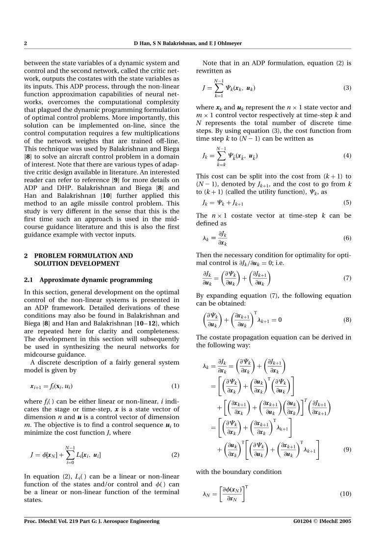
2 D Han, S N Balakrishnan, and E J Ohlmeyer

Proc. IMechE Vol. 219 Part G: J. Aerospace Engineering G01204 # IMechE 2005

Note that the second term on the right-hand side willadd up to zero on the optimal trajectory.

2.2 General procedure for finite time problemsusing adaptive critics

For finite-time (or finite-horizon) problems, thesolution with neural networks evolves in two stages.Note that since the terminal conditions are givenat the last stage, the solution proceeds backwards.

2.2.1 Synthesis of last network

1. Note that lN ¼ ½@f(xN )=@xN �T. For various

random values of xN, lN can be calculated.2. Use the state propagation equation (1) and

optimality condition in equation (8) to calculateuN21 for various xN21 by randomly selecting xNand the corresponding lN from step 1.

3. With uN21 and lN, calculate lN21 for various xN21

by using the costate propagation equation (9).4. Train two neural networks. For different values

of xN21, the uN21 network outputs uN21 withthe training data coming from step 2. The lN21

network outputs lN21 where the training datacomes from step 3. This then gives the optimalcontrol and costates for various values of thestate at stage (N2 1).

2.2.2 Other networks

1. Assume different values of states at xN22 at stage(N2 2) and pick a random network (or initializedwith uN21 network), called the uN22 network, tooutput uN22. Use uN22 and xN22 in the statepropagation equation (1) to obtain xN21. InputxN21 to the lN21 network to obtain lN21. UsexN22 and lN21 in the optimality condition inequation (8) to obtain target uN22. Use this tocorrect the uN22 network. Continue this processuntil the absolute value of the relative changein the output, uN22, between two successive iter-ations is less than 0.01. At this point, this uN22

network is assumed to yield the optimal uN22.2. Using a random xN22, output the control uN22

from the uN22 network. Use these xN22 anduN22 to obtain xN21 and input xN21 to the lN21

network to generate lN21. Use xN22, uN22 andlN21 in equation (9) to obtain the optimal lN22.Train a lN22 network with xN22 as input andobtain the optimal lN22 as output.

3. Repeat the last two steps with i ¼ N2 1,N2 2, . . . , 0, until u0 is obtained.

A schematic of the network development ispresented in Fig. 1.

3 MIDCOURSE GUIDANCE IN A VERTICALPLANE

3.1 Derivation of the optimal trajectory shapingguidance law

The physics and the mathematical model of themidcourse guidance problem are presented in thissection. The basic optimal guidance problem isposed and a simplified cost function is developedto obtain tractable solutions. A discrete formulationfor use with the neural networks is also developed.

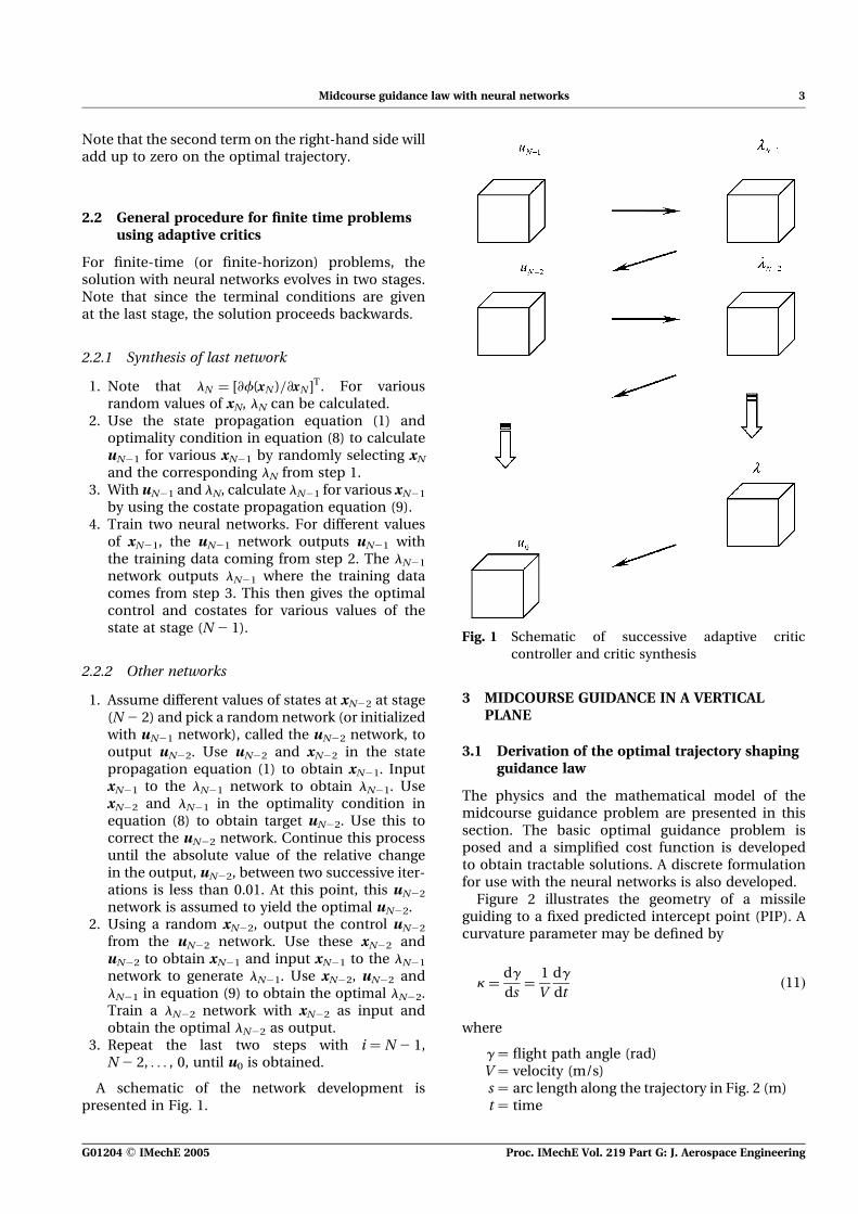
Figure 2 illustrates the geometry of a missileguiding to a fixed predicted intercept point (PIP). Acurvature parameter may be defined by

k ¼dg

ds¼

1

V

dg

dtð11Þ

where

g ¼ flight path angle (rad)V ¼ velocity (m/s)s ¼ arc length along the trajectory in Fig. 2 (m)t ¼ time

Fig. 1 Schematic of successive adaptive critic

controller and critic synthesis

Midcourse guidance law with neural networks 3


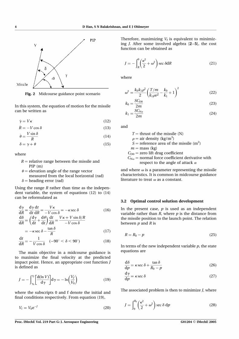
In this system, the equation of motion for the missilecan be written as

_g ¼ Vk ð12Þ

_R ¼ �V cos d ð13Þ

_u ¼V sin d

Rð14Þ

d ¼ gþ u ð15Þ

where

R ¼ relative range between the missile andPIP (m)

u ¼ elevation angle of the range vectormeasured from the local horizontal (rad)

d ¼ heading error (rad)

Using the range R rather than time as the indepen-dent variable, the system of equations (12) to (14)can be reformulated as

dg

dR¼

dg

dt

dt

dR¼

Vk

�V cos d¼ �k sec d ð16Þ

dd

dR¼

dg

dtþ

du

dt

� �dt

dR¼

Vkþ V sin d=R

�V cos d

¼ �k sec d�tan d

Rð17Þ

dt

dR¼ �

1

V cos dð�908 , d , 908Þ ð18Þ

The main objective in a midcourse guidance isto maximize the final velocity at the predictedimpact point. Hence, an appropriate cost function Jis defined as

J ¼ �

ðgfg0

dðlnV Þ

dg

� �dg ¼ � ln

Vf

V0

� �ð19Þ

where the subscripts 0 and f denote the initial andfinal conditions respectively. From equation (19),

Vf ¼ V0e�J ð20Þ

Therefore, maximizing Vf is equivalent to minimiz-ing J. After some involved algebra [2–5], the costfunction can be obtained as

J ¼ �

ð0

R

k2

2þ v2

� �sec ddR ð21Þ

where

v2 ¼k0k1r

2

2

T=m

k1rv2�k0

k1þ 1

� �2

ð22Þ

k0 ¼SCD0

2mð23Þ

k1 ¼SCNa

2mð24Þ

and

T ¼ thrust of the missile (N)r ¼ air density (kg/m3)S ¼ reference area of the missile (m2)m ¼ mass (kg)

CD0 ¼ zero lift drag coefficientCNa ¼ normal force coefficient derivative with

respect to the angle of attack a

and where v is a parameter representing the missilecharacteristics. It is common in midcourse guidanceliterature to treat v as a constant.

3.2 Optimal control solution development

In the present case, p is used as an independentvariable rather than R, where p is the distance fromthe missile position to the launch point. The relationbetween p and R is

R ¼ R0 � p ð25Þ

In terms of the new independent variable p, the stateequations are

dd

dp¼ k sec dþ

tan d

R0 � pð26Þ

dg

dp¼ k sec d ð27Þ

The associated problem is then to minimize J, where

J ¼

ðR0

0

k2

2þ v2

� �sec d dp ð28Þ

Fig. 2 Midcourse guidance point scenario



The Hamiltonian, H, for this problem is defined as [6]

H ¼ Lþ l1dd

dpþ l2

dg

dp

¼ v2 þk2

2

� �sec dþ l1 k sec dþ

tan d

R0 � p

� �þ l2k sec d ð29Þ

where li are the Lagrangian multipliers (costates)corresponding to the Hamiltonian in equation (29).The costate propagation equations are obtained as

_l ¼ ½ _l1; _l2�T¼ �

@H

@d;@H

@g

� �Tð30Þ

_l1 ¼ �@H

@d

¼ � v2 þk2

2

� �sec d tan d� l1 k sec dþ

sec2 d

R0 � p

� �� l2k sec d tan d ð31Þ

_l2 ¼ �@H

@g¼ 0 ) l2 ¼ C0 ð32Þ

For optimality, control k satisfies

@H

@k¼ 0 ð33Þ

Equation (33) leads to

k sec dþ l1 sec dþ l sec d ¼ 0 ð34Þ

From equation (34), an expression for the control kis obtained as

k ¼ �l1 � l2 ¼ �l1 � C0

The boundary conditions are:

at t0 or p ¼ 0:

dðp0Þ ¼ d0; gðp0Þ ¼ g0

at tf or p ¼ R0:

dðpfÞ ¼ 0; gðp0Þ ¼ gf

In order to use the discrete adaptive critic basedneural network solutions, it is necessary to discretizethe equations for the state and optimal control.Note that Euler’s method [13] is used to integratethe continuous form of differential equationsbetween the time-steps by converting it to a dis-crete-time problem as described below.

State equations:

dkþ1 ¼ dk þ kk sec dk þtan dk

R0 � pk

� �Dpk ð35Þ

gkþ1 ¼ gk þ kk sec dkDpk ð36Þ

Cost function:

min J ¼XN�1

k¼0

v2k þ

k2k

2

� �sec dkDpk ð37Þ

Define the Hamiltonian:

Hk ¼ l1;kþ1dkþ1 þ l2;kþ1gkþ1 þ v2k þ

k2k

2

� �sec dkDpk

¼ l1;kþ1 dk þ kk sec dk þtan dk

R0 � pk

� �Dpk

� �þ l2;kþ1ðgk þ kk sec dkDpkÞ

þ v2k þ

k2k

2

� �sec dkDpk ð38Þ

Costate equations:

l1;k ¼@Hk

@dk

¼ l1;kþ1 þ l1;kþ1 kk sec dk tan dk þsec2 dk

R0 � pk

� �Dpk

þ l2;kþ1kk sec dk tan dkDpk

þ v2k þ

k2k

2

� �sec dk tan dkDpk ð39Þ

l2;k ¼@Hk

@gk¼ l2;kþ1 ð40Þ

Optimality control condition:

@Hk

@kk¼ 0 ) kk ¼ �l1;kþ1 � l2;kþ1 ð41Þ

Boundary conditions:

p0 ¼ 0; d0; g0 are known

pN ¼ R0; dN ¼ 0; gN are fixed value

Note that Dp is the step size and k denotes the stage.

4 DEVELOPMENT OF NEURAL NETWORKSOLUTIONS

In this paper, neurocontrollers are obtained for bothfixed final flightpath angle and flexible flightpathangle. After discretizing the system equation, theindependent variable p is divided into appropriate



steps. During each period, two neural networks,namely the ‘action’ network, which represents thestate feedback guidance law and outputs control k,and another network called the ‘critic’ network,which represents the supervisory model outputscostates l1 and l2, are synthesized. The trainedaction networks which are cascaded together willform the optimal guidance law when implementedin real-time.

4.1 Procedure to train neural networks

For ‘finite-time’ (or finite-horizon) problems, the‘time’ (independent) is fixed. In midcourse guidance,the independent variable p is a value that is deter-mined by tactical requirements. Here, according tothe Navy specification, pN is chosen as 97.2 km (60miles). Assume p is divided into N21 fragmentedperiods and the networks are indexed against theseperiods. Then there are N steps in total. The networksare synthesized backwards in this formulation. Thisprocedure includes two stages. A schematic of thenetwork development is presented in Fig. 1.

4.1.1 Synthesis of the last network

1. Randomly pick dN�1. Since dN ¼ 0, given DpN�1,from state equation (35), k�N�1 is obtained.

2. Since gN is fixed, input dN�1 and kN�1 intoequation (36) and gN�1 can be obtained.

3. Train a network denoted as k(N � 1). The inputsare state dN�1 and gN�1, and the target is k�N�1.Train this network until a pre-specified errortolerance is satisfied.

4. Pick dN�1 and gN�1. Use the k(N � 1) network toobtain kN�1. Pick l1,N or l2,N and together withkN�1 compute l2,N or l1,N from equation (41).

5. Input l1,N , l2,N , kN�1, DpN�1, dN�1 and vN�1 intoequations (39) and (40) to obtain l�1,N�1 andl�2,N�1.

6. Train a network called l(N � 1). The inputs arestate dN�1 and gN�1 and the targets are l�1,N�1

and l�2,N�1. Train this network until a specifiederror performance is satisfied.

4.1.2 Synthesis of other networks

1. Determine DpN�2, pick dN�2 and gN�2, input intothe k(N � 1) network to obtain kN�2.

2. Input dN�2, gN�2, kN�2 and DpN�2 into equations(35) and (36) to obtain gN�1 and dN�1.

3. Input gN�1 and dN�1 into the l(N � 1) network toobtain l1,N�1 and l2,N�1.

4. Input l1,N�1 and l2,N�1 into equation (41) toobtain k�N�2.

5. Train a k(N � 2) network with inputs dN�2 andgN�2 and target k�N�2 until convergence is reached.

6. Input dN�2 and gN�2 into the k(N � 2) network toobtain kN�2.

7. Input dN�2, gN�2 and kN�2 into equations (35)and (36) to obtain gN�1, dN�1.

8. Input dN�1 and gN�1 intothe l(N � 1) network toobtain l1,N�1 and l2,N�1.

9. Input l1,N�1, l2,N�1, kN�2, dN�2 and gN�2 intoequations (39) and (40) to obtain target l�1,N�1

and l�2,N�1.10. Train a l(N � 2) network with inputs dN�2

and gN�2 and targets l�1,N�1 and l�2,N�1 until con-vergence is reached.

11. Repeat the process 1 to 10 with N¼N2 1 untilp0 ¼ 0 is reached.

Note that for this method to work in real-time,the procedure is very simple. The control networks(k networks) have the states d and g at differentsteps as inputs and the guidance variable k as theoutput. Assume any d0 and g0 (within the trainedscope), use the k(0) network to find k0 and integrateto get d1 and g1 until p1 is reached. Then input d1 andg1 into the k(1) network to get k1 and integrate toget d2 and g2 until p2 is reached. Continue until pN ¼

R0 is reached.

5 NUMERICAL RESULTS

5.1 Fixed final flightpath angle

Results from simulations using the neural networkapproach and the shooting method [6] are presentedin this section. The desired final states for the mid-course missile were fixed at zero for the headingerror d, zero for the flightpath angle g and sixtymiles for the range. The parameter v was set at0.000 04. A feedforward neural network with threelayers with a hyperbolic tangent sigmoid a log-sigmoid, and a linear activation function is usedfor the controller network as well as for the criticnetwork. The number of neurons is 4 in the firstand second layers and 1 in the third layer. TheLevenberg–Marquardt training algorithm is used intraining both the action and the critic neural net-works. It needs to be pointed out that these choicesfor the structure and training method were notchosen for any specific reason. The results showedthat the choices were adequate. In the trainingprocess, Euler’s method is used to integrate thestate equations between the steps defined by theintervals in the independent variable. The divisionsin the training scope of the initial flight path angleand the heading errors are presented in Fig. 3.After training, there are 62 pairs of networks to cover97.2 km. These studies, however, were carried outin British units with a maximum range of 60 miles.



In order to keep the same scale with properdivisions, the range information is plotted with ascale factor of 1.62 so that the maximum value is60 units.

The sampling period through the network syn-thesis was selected based on the accuracy of compu-tations. It is important to state that the networksare not placed evenly with regard to the indepen-dent variable. The physics of the problem plays animportant role in this aspect. If the step size istaken to be large (in order to keep the number ofnetworks small), the iterative process between theupper level costate network and the lower levelcontroller network would not converge. This isbecause the initial states for the lower level andthe resulting control (which is really initialized withthe upper level controller weights) would place thepropagated state much beyond the level of therange for which the upper level costate networkwas synthesized. It should be noted that this meansthat the optimal guidance law has been obtainedfor any range from 0 to 97.2 km to reach the pre-dicted impact point with the maximum velocityand with zero heading error and zero flightpathangle.

Three-dimensional plots of trajectories obtainedwith the neural networks are presented in Fig. 4.The two costates (Lagrangian multipliers) are plottedin Fig. 5. The corresponding history of the control

variable k is presented in Fig. 6. In order to verifythe optimality of the neural network results, thesame initial conditions were used and the shootingmethod was used 36 times by solving each singleproblem separately. These results were found to bealmost identical with the neural network results.A unique aspect of this development is that theneural networks are used as a computational toolto solve the optimal guidance problem directlyrather than to train it and use the generalizationproperty of the neural networks. If a traditionalmethod such as a shooting method is employed asa tool, the optimal control problem would have tobe solved iteratively for every set of initial conditions.Therein is the computational advantage of the adap-tive critic approach; the same set of neural networksembed countably infinite optimal solutions to themidcourse guidance problem with any initial con-dition from Fig. 4 or with any range up to 97.2 km.In other words, a large number of shooting methodsolutions are embedded in a set of networkswithout as much computational effort.

5.2 Variable final flightpath angles

The results presented in the previous section wereobtained for a fixed final flightpath angle gf ¼ 0.In order to capture the target in a different situation,it is necessary for the missile to reach the PIP at

Fig. 3 Training scope of initial d and g



Fig. 5 Costate l histories (NN)

Fig. 4 Histories of d and g (NN)



different final flighpath angles or from different atti-tudes. If one set of networks for each final flightpathangle were to be used, there would be several net-works corresponding to different specified finalflightpath angles. For any other final flightpathangle, two successive neural network controllershave to be interpolated. This is not practical in realimplementation. Therefore the neural network’sinherent universal learning or mapping ability isexploited in this study and a single network wasused to output costates for different final flightpathangles at any stage. The way to do this was to aug-ment the final flightpath path angle as anotherinput and target during neural network training.In this study, the final flightpath angle range wasfrom 608 to 908 with an interval of 58 as the trainingscope. The initial heading error and flightpathangle scope remain the same as before. The rangeand the parameter v were also assumed to besame. InQ1 this new design a feedforward neuralnetwork was chosen with all three layers with linearactivation functions for the controller network aswell as for the critic network. The numbers ofneurons are 8 in the first layer and 8 in the secondlayer for both the controller and critic networks.A Levenberg–Marquardt algorithm was still used intraining both the action and the critic neural

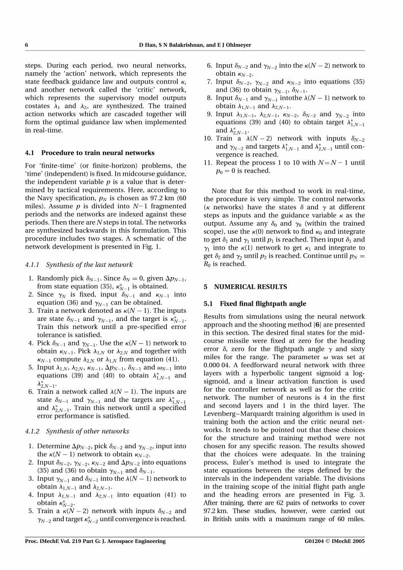
networks. This time 79 pairs of networks were used.The results of the neural network controller fora set of initial conditions and desired final flightpathangles are plotted in Figs 7 to 11. It can be seen thateven with variable final flightpath angles, the neuralnetworks capture the optimal control and the trajec-tories very well. The errors of g between the neuralnetworks and the shooting method are plotted inFigs 12 to 14. The maximum error for g is about4.38 and the error approaches zero at the end. Theerrors are attributed to the different step sizes.The larger error trajectories are those that have asmaller initial flightpath angle and heading anglebut a larger negative final flightpath angle. Thereason is that it is more difficult to shape a low, flattrajectory at the final stage.

There may be some concern over the number ofneural networks needed to synthesize the controllerin this proposed approach. However, an alternatescheme can be devised to reduce the numberof neural networks used in controller synthesis.The independent variable could be used as an extrainput to the neural networks in addition to thestates. While this scheme would increase thenumber of neurons, the number of networks forthe controller as well as for the costates would bereduced to one.

Fig. 6 Kappa histories (NN)



Fig. 7 d histories for different gf (NN)

Fig. 8 g histories for different gf (NN)



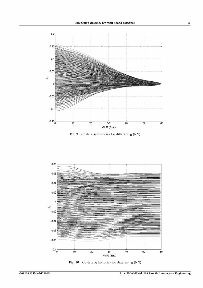
Fig. 9 Costate l1 histories for different gf (NN)

Fig. 10 Costate l2 histories for different gf (NN)



Fig. 11 Kappa histories for different gf (NN)

Fig. 12 Kappa errors for different gf (NN with shooting)



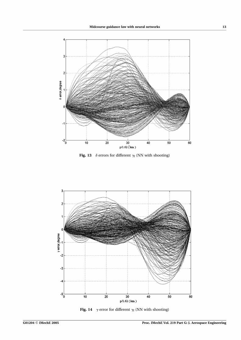
Fig. 13 d errors for different gf (NN with shooting)

Fig. 14 g error for different gf (NN with shooting)



6 CONCLUSIONS

A neural network approach to solve optimal mid-course guidance problems has been presentedin this study. This approach solves non-linear gui-dance/control problems without having to makelinearizing approximations to the model. The resultsshow that the adaptive critic-based neural networkspresent a powerful computational approach to thefinite-horizon class of optimal control problems.

ACKNOWLEDGEMENT

This research was partly supported by a grant fromthe Naval Surface Warfare Center, Dahlgren, Virginia,and a grant from the National Science Foundation.

REFERENCES

1 Cherry, G. A general, explicit, optimizing guidance lawfor rocket-propelled spaceflight. In Astrodynamics,Guidance and Control Conference, 24–26 August,1964, AIAA paper 64-638.

2 Lin, C. F. and Tsai, L. L. Analytical solutions of optimaltrajectory-shaping guidance. Am. Inst. Aeronaut.Astronaut. J Guidance, Control and Dynamics,January–February 1987, 10(1).

3 Lin, C. F. Modern Navigation, Guidance, and Con-trol Processing, 1991, pp. 562–583, (Prentice-Hall,Englewood Cliffs, New Jersey).

4 Reifler, F. Curvature guidance algorithm derivation.RCA Memo TI 7830, Moorestown, New Jersey, 27 May1979, pp. 19–43.

5 Serakos, D. and Lin, C. F. Linearized kappa guidance.Am. Inst. Aeronaut. Astronaut. J Guidance, Controland Dynamics, September–October 1995, 18(5).

6 Bryson, A. E. and Ho, Y. C. Applied Optimal Control,1975 (Halsted Press).

7 Werbos, P. J. Approximate dynamic programming forreal-time control and neural modeling. In Handbookof Intelligent Control (Eds D.A. White and D. Sofge),1992 (Multiscience Press).

8 Balakrishnan, S. N. and Biega, V. Adaptive critic basedneural networks for aircraft optimal control. Am. Inst.Aeronaut. Astronaut. J Guidance, Control andDynamics, July–August 1996, 19(4), 893–898.

9 Prokhorov, D. V. and Wunsch II, D. C. Adaptive criticdesigns. IEEE Trans. Neural Networks, 1997, 8(5),997–1007.

10 Han, D. and Balakrishnan, S. N. Adaptive critic basedneural network for agile missile control. Am. Inst. Aero-naut. Astronaut. J Guidance, Control and Dynamics,March 2002, 25(2).

11 Han, D. and Balakrishnan, S. N. Robust adaptive criticbased neural network for control-constrained agilemissile control. In American Control Conference, SanDiego, California, June 1999, 2600–2604.

12 Han, D. and Balakrishnan, S. N. Robust adaptive criticbased neural network for speed-constrained agilemissile control. IEEE Trans. Control System Technol.,July 2002, 10(4), 481–489.

13 Philips, G. M. and Taylor, P. J. Theory and Applica-tions of Numerical Analysis, 1973 (Academic Press,New York).

APPENDIX

Notation

CD0 zero lift drag coefficientCNa normal force coefficient derivative with

respect to the angle of attack a

f linear or non-linear function of x and uH Hamiltonian, a quantity defined in optimal

control theoryJ cost function to be minimizedL linear or non-linear function of x and u in

the cost functionm mass (kg)N total number of stagesp distance from the missile position to the

launch pointR relative range between the missile and the

predicted impact point (PIP)s arc length along the trajectory (m)S reference area of the missile (m2)T thrust of the missile (N)u m-dimensional control vectorV velocity (m/s)x n-dimensional state vector

a angle of attack (rad)g flight path angle (rad)d heading error (rad)u elevation angle of the range vector

measured from the local horizontal (rad)k curvature parameterl costate, a term defined in optimal control

theoryn Poisson ratior air densityf terminal cost in a cost functionC stage dependent cost functionv parameter representing missile

characteristics

Subscripts

f final conditionk stage0 initial condition



IMECHE

JOURNAL…JAE.... ARTID… G01204

TO: CORRESPONDING AUTHOR

AUTHOR QUERIES - TO BE ANSWERED BY THE AUTHOR

The following queries have arisen during the typesetting of your manuscript. Please answer these queries.

Q1 Please check the edit of the sentence.

Q

Journal of Aerospace Engineering Proceedings of the Institution of Mechanical Engineers Part G OFFPRINTS/JOURNAL ORDER FORM To ensure that you receive the offprints or Journal you require please return this form with your corrections. Manuscript Number: G/2004/000012 Number of pages: 14 Authors: Donchen Han, S N Balakrishnan and Ernest J Ohlmeyer If you would prefer to receive a free copy of the Journal issue instead of 25 free offprints please indicate below: Quantity 1 copy of the 25 offprints Journal issue Cost free free Please supply ...................... offprints / 1 copy of the Journal issue* and forward to the following address: *Delete as appropriate Professor S N Balakrishnan c/o Mr Ming Xin Postdoctoral Research Fellow Department of Mechanical and Aerospace Engineering University of Missouri-Rolla Rolla MO 65401 USA Quotations for additional reprints will be provided on request.

Documents

SPECIAL ISSUE PAPER 1 Midcourse guidance law …web.mst.edu/~autosys/papers/002.pdfMidcourse guidance law with neural networks D Han, S N Balakrishnan , and E J Ohlmeyer† Department