Embed Size (px)
Citation preview

Special Topic – Item 3
Quarterly National Accounts
Giovanni SavioStatistics Coordination Unit, UN-ESCWA
Workshop on National AccountsCairo, 19-21 December 2006

Objectives of presentation
1. Background on QNA
2. General principles for QNA
3. Coverage, sources and methods for QNA estimation
4. Seasonality and seasonal adjustment of QNA

Importance of QNA
There is no reference in 1993 SNA to QNA, and they are not considered in the revision process
So, are QNA important? If yes, why?
“The importance of quarterly accounts derives essentially from the consideration that they are the only coherent set of indicators, available with a short time-lag, able to provide a short-term overall picture of both non-financial and financial economic activity” (ESA 1995, § 12.02)

Importance of QNA
QNA have been deeply considered in the Handbook on Quarterly National Accounts by Eurostat (1999), and in the Quarterly National Accounts Manual by IMF (2001)
Furthermore, a chapter of the European System of Accounts 1995 (ESA 1995) by Eurostat is dedicated to QNA
The main purpose of QNA is to provide a picture of current economic developments that is more timely than that provided by ANA, and more comprehensive and coherent than that provided by individual short-term indicators

Importance of QNA
To meet this purpose, QNA should be timely, coherent, accurate, comprehensive, and reasonably detailed
If QNA fulfill these criteria, they are able to serve as a framework for assessing, analyzing, and monitoring current economic developments

Importance of QNA
By providing time series of quarterly data on macroeconomic aggregates in a coherent accounting framework, QNA allow analysis of the dynamic relationships between these aggregates (particularly, leads and lags)
Thus, QNA provide the basic data for short-term business
cycle analysis and for economic modelling, control and forecasting purposes. As such, they can be of great use for policy analysts, researchers and policy-makers

Importance of QNA
QNA can be seen as positioned between ANA and specific short-term indicators. QNA are commonly compiled by combining ANA data with short-term source statistics, thus providing a combination that is more timely than that of the ANA and that has increased information content and quality compared with short-term source statistics
“Quarterly economic accounts form an integral part of the system of national accounts. … The quarterly economic accounts constitute a coherent set of transactions, accounts and balancing items, defined in both the non-financial and financial domains, recorded on a quarterly basis. They adopt the same principles, definitions and structure as the annual accounts” (ESA 1995, § 12.01)

Importance of QNA
QNA are usually available within two-three months after the reference quarter, or even less in case of flash estimates. ANA, on the other hand, are produced with a considerable time lag, often greater than six months
Thus, ANA do not provide timely information about the current economic situation, which hampers monitoring the business cycle and the timing of economic policy aimed at affecting the business cycle
ANA are less suitable than QNA for business cycle analyses because annual data mask short-term economic developments
Importance of QNA
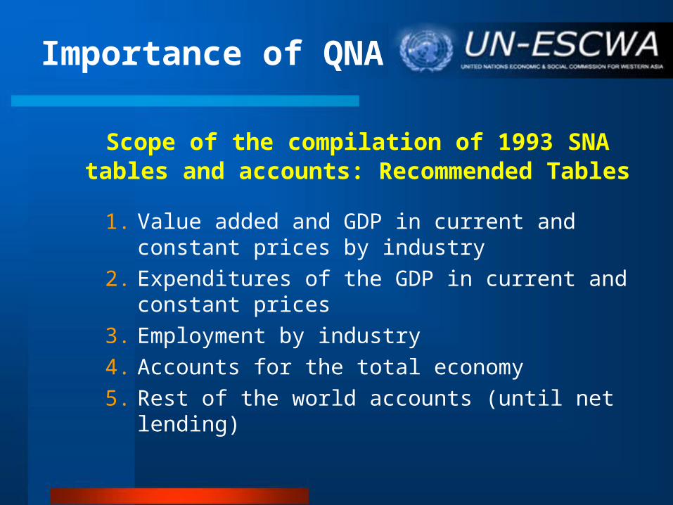
Scope of the compilation of 1993 SNA tables and accounts: Recommended Tables
1. Value added and GDP in current and constant prices by industry
2. Expenditures of the GDP in current and constant prices
3. Employment by industry
4. Accounts for the total economy
5. Rest of the world accounts (until net lending)

General principles related to QNA
To avoid confusion about interpreting economic developments, it is imperative that the QNA are consistent with the ANA
Differences in growth rates and levels between QNA and ANA would perplex users and cause uncertainty about the actual situation
“Since quarterly accounts adopt the same framework as annual accounts they have to be consistent over time with them. This implies, in the case of flow variables, that the sum of the quarterly data is equal to the annual figures for each year” (ESA 1995, § 12.06)

General principles related to QNA
Transparency of QNA is a fundamental requirement of users, and is particularly pertinent in dealing with revisions
To achieve transparency, it is important to provide users with documentation regarding the source data used, the way they are adjusted and compilation processes
This will enable users to make their own judgments on the accuracy and the reliability of the QNA and will pre-empt possible criticisms of data manipulation

General principles related to QNA
In addition, it is important to inform the public at large about release dates so as to prevent accusations of manipulative timing of releases
Revisions in QNA can be due to a number of factors, both technical (seasonal adjustment, benchmarking etc.) and linked to data sources
There is often a trade-off between timeliness and accuracy of published data: the request by users of prompt information can generate increased revisions later on
Revisions provide the possibility to incorporate new and more accurate information into the estimates, and thus to improve their accuracy

General principles related to QNA
Delaying the implementation of revisions may cause later revisions to be greater
Not incorporating known revisions actually reduces the trustworthiness of data because the data do not reflect the best available information
Although the scale of data revision and the reliability of the estimates are closely linked, they are quite different concepts: a time series can be never revised, but at the same time be completely unreliable
A final judgement on reliability depends on the reliability of basic data sources and the estimation methods used
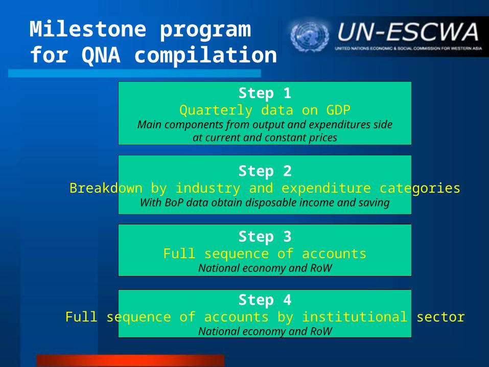
Milestone programfor QNA compilation
Step 1Quarterly data on GDP
Main components from output and expenditures sideat current and constant prices
Step 2Breakdown by industry and expenditure categories
With BoP data obtain disposable income and saving
Step 3Full sequence of accounts
National economy and RoW
Step 4Full sequence of accounts by institutional sector
National economy and RoW

Data sources for QNA estimates
Ideally, ANA should be derived as the sum (or average for stock variable ) of the corresponding quarterly data
Unfortunately, sources for ANA are generally different, more exhaustive, reliable and comprehensive than the corresponding ones for QNA
In many cases, data are collected only at the lower (annual) frequency, and at the higher frequency (quarterly or monthly) only ‘indicators’ or proxies are available, if any
This situation implies that ANA play a leading role and serve as a reference benchmark for QNA, and QNA generally ‘follow’ annual estimates

Data sources for QNA estimates
Therefore, an important aspect of the quality of QNA is the closeness of the indicators used for QNA estimation to the corresponding sources used for the estimation of ANA
The basic principle in selecting and developing QNA sources is to obtain indicators that best reflect the items being measured
In some cases, source data are available in a form ready for use in the ANA or QNA with little or no adjustment. In other cases, the source data will differ from the ideal in some way, so that the source data will need to be adjusted, and benchmarking can play a major role in the adjustment

Data sources for QNA estimates
In some cases, the same sources that are used annually or for the main benchmark years may also be available on a quarterly basis, most commonly foreign trade, central government, and financial sector data
More commonly, QNA data sources are more limited in detail and coverage than those available for the ANA because of issues of data availability, collection cost, and timeliness
For each component, the available source that best captures the movements (rates of growth) in the target variable both in the past and in the future constitutes the best indicator.

Data sources for theproduction approach
The production approach is the most common approach to measuring quarterly GDP
As in the other approaches, the availability and reliability of indicators can substantially differ from one country to another
The production approach involves calculating output, intermediate consumption and value added at current prices as well as in volume terms by industry
Because of definitional relationships, if two out of output, intermediate consumption, and value added are available, the third can be derived residually. Similarly, if two out of values, prices, and volumes are available, the third can be derived

Value and volume indicators for GDP by industry
Cat. Description Main Indirect Sources
A+B Agriculture, hunting, forestry and fishing
Harvesting data; Quantity of meat produces and prices from abattoirs; Number of animals slaughtered; Quantity of timbers felled; Fodder and consumption of fertilizers; Value and size of catches; Fishermen’s landing
C+D+E Industry, including energy Industrial production index; Qualitative business surveys; Employment data
F Construction Employment data; Supply of building materials
G+H+I Wholesale and retail trade, repairs, hotels and restaurants, transport and communications
Turnover statistics; Volume of goods transported; Nights spent in hotels; Number of passengers; Subscribers to TV services
J+K Financial, real estate, renting and business activities
Value of loans/deposits; Interest rates spreads; Expenditures of households on dwelling rents;
Industry indicators
L to P Other service activities Number of employees; Wages and salaries

Value and volume indicators for GDP by industry
280000
290000
300000
310000
320000
330000
340000
80
85
90
95
100
1990 1995 2000 2005
VINDUS IPI

Value and volume indicators for GDP by type of expenditure
Description Main Indirect Sources
Household final consumption expenditure Sales or revenues statistics; Surveys of retailers and service providers; VAT systems; Turnover index; Household budget survey; Commodity flow approach; Cars registration; Business consumer qualitative surveys; Employment/earnings in the activities concerned; Population; Radio and TV licences; Overnight stays; Traffic indicators; Changes in number of dwellings
General government consumption expenditure
Data from government accounts; Wage and salaries statistics
Gross fixed capital formation Commodity flow approach; Value/volume of work done by capital goods producers; Index of construction output; Hours worked/number of employees; Capital outlays by purchasers of capital goods
Change in inventories Business surveys; Information from holders of stocks; Qualitative business surveys
Exports and imports of goods and services Customs (values and unit values) and BoP data
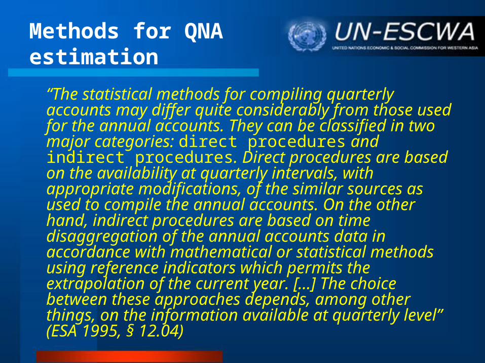
Methods for QNA estimation
“The statistical methods for compiling quarterly accounts may differ quite considerably from those used for the annual accounts. They can be classified in two major categories: direct procedures and indirect procedures. Direct procedures are based on the availability at quarterly intervals, with appropriate modifications, of the similar sources as used to compile the annual accounts. On the other hand, indirect procedures are based on time disaggregation of the annual accounts data in accordance with mathematical or statistical methods using reference indicators which permits the extrapolation of the current year. […] The choice between these approaches depends, among other things, on the information available at quarterly level” (ESA 1995, § 12.04)

The use of informationin QNA estimation
Existing data sources
Are there quarterly data for the aggregate and are they coherent with 1993 SNA?
Yes
NoDo they cover the whole period?
Are close to 1993 SNA?
Are suitable for use in models?
Stage 1a Use data directly(with or without grossing up)
Stage 1b Use statistical models
Stage 2 Make suitable adjustments and use the derived data
Stage 3 Build models based on the indicators
Stage 4 Use another method
Stage 5 Use trend or modelswithout indicators
Look fornew data Are coherent with 1993 SNA?
Use flash estimates
Yes
Yes
No
No
Yes
Yes
No
No
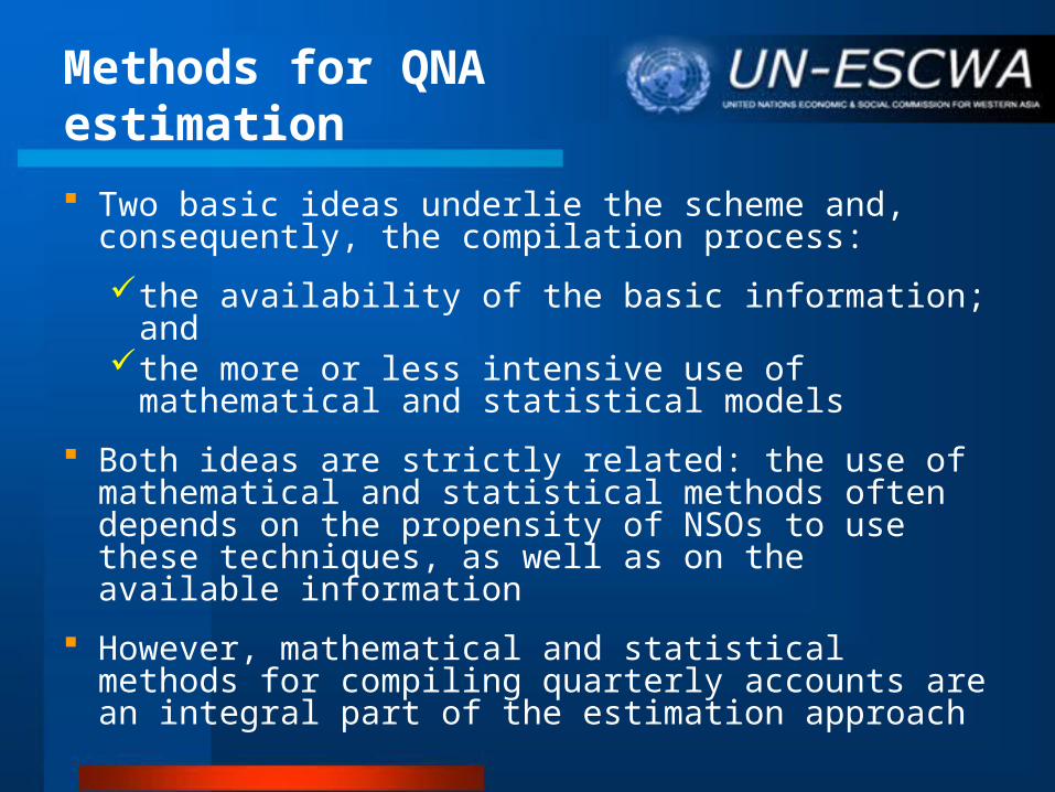
Methods for QNA estimation
Two basic ideas underlie the scheme and, consequently, the compilation process:
the availability of the basic information; and the more or less intensive use of mathematical and
statistical models
Both ideas are strictly related: the use of mathematical and statistical methods often depends on the propensity of NSOs to use these techniques, as well as on the available information
However, mathematical and statistical methods for compiling quarterly accounts are an integral part of the estimation approach

Methods for QNA estimation
A minimum amount of actual data is necessary to provide meaningful QNA figures
Without this minimum amount, a reliable quarterly system cannot be established
As the availability of a complete set of reliable surveys at the quarterly level is unlikely for most countries, we concentrate here on some important indirect methods for estimation of QNA

Indirect estimationmethods
We distinguish between methods that do not make use of any information (purely mathematical methods), and methods that use related time series as indicators for the unknown quarterly series
Purely mathematical methods
Simple extrapolation Denton Chow & Lin (regression methods)
No indicators
Indicators
Simple extrapolation
1
1
1
1 , with ,
t
ttt
t
ttttt x
xxx
y
yyyxy
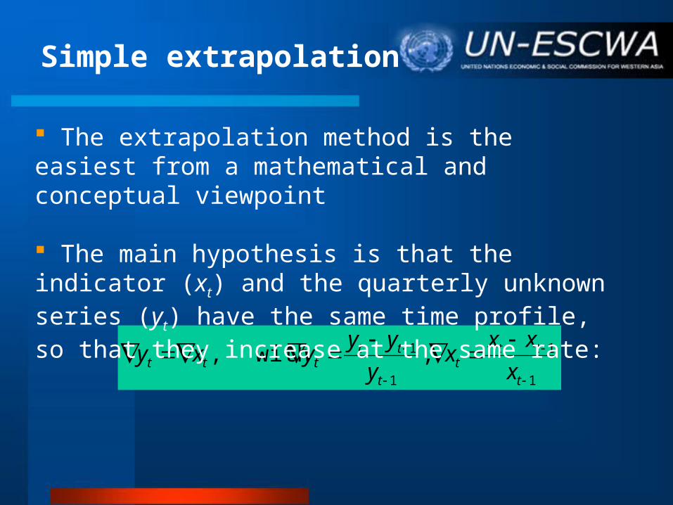
The extrapolation method is the easiest from a mathematical and conceptual viewpoint
The main hypothesis is that the indicator (xt) and the quarterly unknown series (yt) have the same time profile, so that they increase at the same rate:

Simple extrapolation
This hypothesis is quite strong as it implies that in all the economic phases the behaviour of the two variables is the same and that there are no lags or leads. In order to respect this hypothesis, the indicator and the quarterly aggregate have to measure exactly the same economic phenomenon
However, if the conditions discussed are respected, the following simple extrapolation formula can be used

Simple extrapolation
1
10111
11
1...1 1
on,substitutiby and,
1
t
iitttt
ttt
xyxxyy
xyy
Then, the problem is represented by the choice of the initial conditions y0. The level of yt+1 depends on the initial conditions, whereas the growth rate of yt is totally independent. This implies that simple extrapolation is a good method for the estimation of growth rates, but not necessarily for the estimation of levels

Simple extrapolation
If a plausible value of y0 has been chosen, the values y1, y2, y3, y4 can be considered as reasonable until the availability of the annual estimates. It is then necessary to run an adjustment procedure (benchmarking) to make the levels for the quarters consistent with the figures for the year
Following the above adjustment, the first quarter of the second year can be estimated starting from a consistent level. In principle, the estimation of y5 should be considered as also being of the correct level
Since the information set used for quarterly accounts is generally different from the set used for annual accounts, even if the estimates for the year t start from a fully consistent set of estimates of the last quarter of year t-1, they are not necessarily correct in level and, when a new annual value becomes available, an adjustment procedure is needed

Benchmarking
Benchmarking is a mathematical procedure that makes the information coming from the high frequency series (quarterly) coherent with the low frequency series (annual)
Annual data provide the benchmark, or the target, for the quarterly data. The sum of quarterly data is consistent with the annual data, but the infra-annual time dynamic is close as much as possible to the time profile of the quarterly indicator
The simplest benchmarking method is given by the benchmark-to-indicator (BI) ratio and the pro-rata distribution of the discrepancies. However, this method generally causes discontinuities (steps) in correspondence of the first quarter of the year

Benchmarking

Benchmarking

Benchmarking
Denton (proportional) method
The basic distribution technique introduces a step in the series, and thus distorts quarterly patterns, by making all adjustments to quarterly growth rates to the first quarter
This step is caused by suddenly changing from one BI ratio to another. To avoid this distortion, the (implicit) quarterly BI ratios should change smoothly from one quarter to the next, while averaging to the annual BI ratios
Consequently, all quarterly growth rates will be adjusted by gradually changing, but relatively similar, amounts

Denton (proportional) method
This is a two-step adjustment method, as it divides the estimation process in two operationally separate phases: preliminary estimation and adjustment to fulfil the annual constraints
The basic version of the proportional Denton benchmarking technique keeps the benchmarked series as proportional to the indicator as possible by minimizing (in a least-squares sense) the difference in relative adjustment to neighbouring quarters subject to the constraints provided by the annual benchmarks
Mathematically, the basic version of the proportional Denton technique can be expressed as

Denton (proportional) method
• The proportional Denton technique implicitly constructs from the annual observed BI ratios a time series of quarterly benchmarked QNA estimates-to-indicator (quarterly BI) ratios that is as smooth as possible
T
2t
2
2
1
1
),...,4,...,2(
constraintunder
min
tt
T
t t
t
t
t
Tyyy
Ay
x
y
x
y

Denton (proportional) method

Denton (proportional) method

Denton (proportional) method

Chow-Lin method
Regression methods are ‘optimal’ one-step methods, as the derivation of quarterly series and the fulfilment of annual constraints are obtained simultaneously
These methods are based on the least-square regression estimates between the annual known data and the annualized quarterly indicator(s)
The simple, linear and static form is the Chow-Lin regression equation
0
4/,...,2,1 , with ,4
1
t
s
stttttt
uE
TsxXuXY

Chow-Lin method
Once the estimates of the parameters are obtained by ordinary least squares, say and , they can be applied to the quarterly indicators to obtain the quarterly unknown values of the dependent series:
Optimal regression methods generally differ regarding the assumptions on ut and the regression model used (static or dynamic)
Ttxy tt ,...,2,1 ,ˆˆ
Seasonality and seasonaladjustment
Due to the periodicity at which they are recorded, quarterly series quite often show short-term movements caused by the weather, habits, legislation, etc., which are usually defined as seasonal fluctuations
These movements tend to repeat them selves in the same period (month or quarter) each year
Although seasonality is an integral part of quarterly data, it may represent an impediment to effective analysis of the business cycle and rates of growth in the last part of the series

Seasonality and seasonaladjustment
• Causes for a seasonal behaviour of time series are numerous:
– Calendar effects The timing of certain public holidays, such as Christmas, Easter, Ramadam, clearly affects some series, particularly those related to production and sells. Also, many series are recorded over calendar months, and as the number of working days varies from one month to another, in a predetermined way, this will cause a seasonal movement in series such as imports or production. The working and trading days problem could also lead to seasonal effects
– Timing decisions Timing of school vacations, ending of university sessions, payment of company dividends, choice of the end of a tax-year are examples of decisions made by

Seasonality and seasonaladjustment
individuals/institutions that cause important seasonal effects, as these events are inclined to occur at similar times each year. They are generally deterministic, or pre-announced
– Weather Actual changes in temperature, rain fall and other weather variables have direct effects on various economic series, such as those related to agricultural production, construction and transportation, and determine seasonal fluctuations
– Expectations The expectation of a seasonal pattern in a variable can cause an actual seasonal effect in that or other variables, since expectations can lead to plans that then ensure seasonality. An example is toy production in expectation of a sales peak during the Christmas period. Without the expectation, the seasonal pattern may still occur but might be of a different shape or nature. Expectations may also arise because it has been noted that the series in the past contained a seasonal pattern

Seasonality and seasonaladjustment
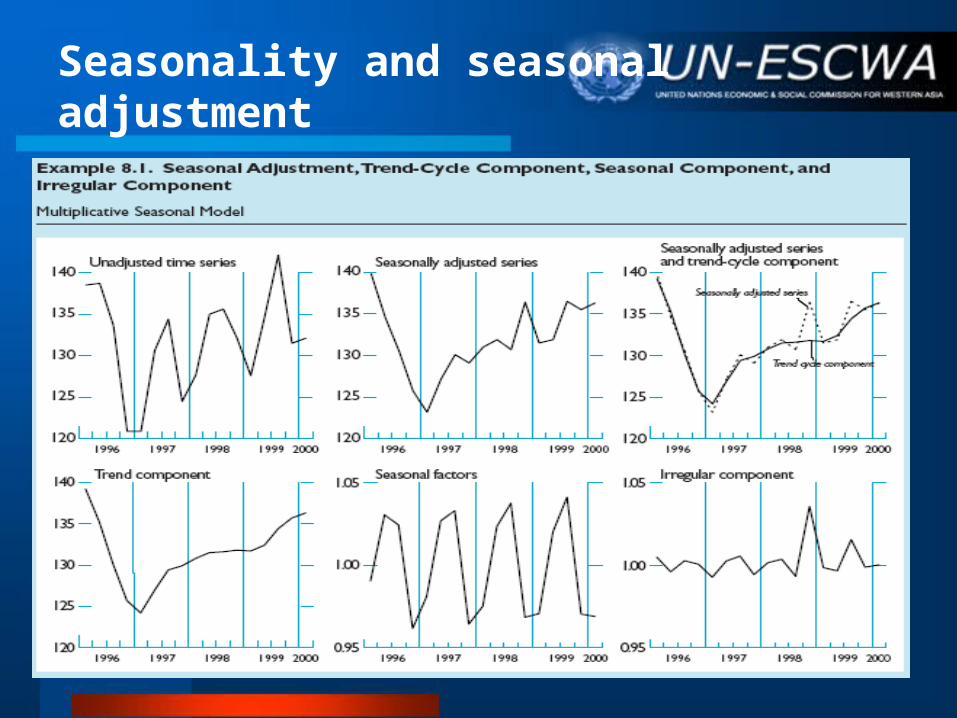
Seasonal adjustment consists in the removal of the seasonal component from the time series
A time series is ideally defined as the sum of some unobserved component: trend, cycle, seasonality and irregular. If the model is additive we have:
TtISCTy ttttt ,...,2,1 ,
Seasonality
Seasonality and seasonaladjustment

Seasonality and seasonaladjustment
How is the seasonal eliminated from the series? Let us consider that for seasonal time series the analysis of standard rates of growth gives misleading results
Instead, the fourth rate of growths can be considered as appropriate
as the fourth difference eliminates in general the seasonal component
1
1
t
ttt y
yyy
4
44
t
ttt y
yyy

Seasonality and seasonaladjustment
Now, by defining the lag operator B we have that:
namely4
44 )1(
,)1(
tttt
tt
yyyBy
yBy
))(1(
)1)(1()1(
with
)1(
,)1(
321
3214
44
4
tttt
tt
tttt
tt
yyyyB
yBBBByB
yyyBy
yBy

Seasonality and seasonaladjustment
The second term in the last formula is called moving average of order 4, and is capable of eliminating (stochastic) seasonality in quarterly time series
Seasonal adjustments programs use more or less extensively these moving averages in order to extract the seasonal component from time series
There are two families of such programs: those based on empirical filters (X-11 type family) and those based on model-based filters (i.e. Tramo-Seats)

Seasonality and seasonaladjustment
The ‘philosophical’ difference between the two families is that:
empirical filter programs use the same filters (moving averages) independently on the time series analysed
in the model-based approach the filters used depend on the characteristics of the series and change accordingly
The difference in terms of performance between the two classes of approaches are in many cases marginal

Seasonality and seasonaladjustment
Seasonal adjustment and benchmarking are part of the same process of estimation of final QNA. They closely interact, a standard sequence of estimation steps being as follows
Seasonaladjustment
Raw quarterly indicator
Seasonally adjustedquarterly indicator
Benchmarking
QNA s.a.
QNA raw

References
1. Eurostat (1999), Handbook on Quarterly National Accounts, Luxembourg: European Communities, available at: http://epp.eurostat.cec.eu.int/portal/page?_pageid=1073,1135281,1073_1135295&_dad=portal&_schema=PORTAL&p_product_code=CA-22-99-781
2. A. M. Bloem, R. J. Dippelsman, and N. O. Maehle (2001), Quarterly National Accounts Manual - Concepts, Data Sources, and Compilation, Washington DC: International Monetary Fund, available at: http://www.imf.org/external/pubs/ft/qna/2000/Textbook/index.htm