Embed Size (px)
Citation preview
7/29/2019 Specialist, Designated Market Makers, Mao_Pagano2011JBF
http://slidepdf.com/reader/full/specialist-designated-market-makers-maopagano2011jbf 1/16
Specialists as risk managers: The competition between intermediated and
non-intermediated markets
Wen Mao, Michael S. Pagano *
Villanova School of Business, Villanova University, Villanova, PA 19085, United States
a r t i c l e i n f o
Article history:Received 15 May 2009
Accepted 12 July 2010
Available online 16 July 2010
JEL classification:
D1
G12
G24
G1
Keywords:
Market microstructure
Specialists
Market makers
Competition
Theory
a b s t r a c t
We develop a model that analyzes competition between a non-intermediated market (such as an elec-tronic communications network) and an intermediated market (such as via the market specialist’s struc-
ture within the NYSE) when both markets are allowed to trade the same securities. Specialists are viewed
as providers of a ‘‘volatility dampening” service, a mechanism for reducing round-trip trading costs, as
well as an ‘‘order execution risk management” service. The economic value of these three specialist ser-
vices is determined by five key factors (the difference in spreads between the two financial market types,
investors’ holding periods, the specialist’s quoted spread in relation to the asset’s price, the relative prob-
ability of executing an order in the intermediated market, and the short-term risk-free rate).
Ó 2010 Elsevier B.V. All rights reserved.
1. Introduction
Securities markets provide important services that go beyond
the specific private benefits of facilitating the exchange of assets
between investors and helping companies raise financial capital.1
In particular, well-functioning financial markets produce a public
good in the form of timely information about the value of numerous
marketable securities which all members of society can use to man-
age scarce resources, allocate funds for investment, and plan for the
future. Given the important externalities and public good attributes
of a securities market, it is not surprising that governments regulate
these financial markets fairly closely and that regulatory activity in
the US has increased over the past 10–15 years.In addition, entirely new trading systems such as electronic
communications networks (ECNs) have also sprung up since the
change in Nasdaq order handling rules during 1997. The ECNs’
market structure is a ‘‘non-intermediated” one because there is
no designated market maker/specialist or dealer that is charged
with maintaining a ‘‘fair and orderly” market for trading stocks
on this type of system.2 In contrast to ECNs, older, more established
stock markets such as the New York Stock Exchange (NYSE) typically
employ an ‘‘intermediated” market model where a market specialist,
or designated market maker, stands ready to use his/her own capital
to maintain a fair and orderly market in the trading of NYSE stocks.3
In fact, the NYSE has rolled out its ‘‘hybrid market” which combines
the traditional floor-based specialist system with the automated
matching and electronic order book systems of Direct+ and NYSE
ARCA.4 Thus, the competition between intermediated and non-inter-
0378-4266/$ - see front matter Ó 2010 Elsevier B.V. All rights reserved.doi:10.1016/j.jbankfin.2010.07.017
* Corresponding author. Tel.: +1 610 519 4389; fax: +1 610 519 6881.
E-mail addresses: [email protected] (W. Mao), michael.pagano@villano-
va.edu (M.S. Pagano).1 See Harris (2003) for a detailed discussion of the private and public benefits of a
financial market and the role of regulation and social welfare in relation to these
benefits.
2 In addition to the ECNs noted above, crossing networks and block trading systems
such as Liquidnet, Pipeline, and ITG’s Posit (commonly referred to as alternativetrading systems, or ATSs), as well as ‘‘dark pools” operated by firms such as Credit
Suisse and Goldman Sachs have also garnered a growing share of the market for
trading US equities.3 Recently, the NYSE has begun to refer to specialists as designated market makers.
For brevity, we use the traditional (and more concise) term, ‘‘specialists”, throughout
this paper when referring to these designated market makers.4 The stated intention of this combination of intermediated and non-intermediated
markets at the NYSE is to provide greater choice to traders and let the customer
decide which of these competing models they prefer. Interestingly, Hendershott and
Moulton (2008) report that the advent of the NYSE Hybrid Market has led to a
significant decrease in specialists’ floor-based participation rates. However, despite
some analysts’ predictions that specialists will become obsolete, there is growing
evidence across many markets around the world (detailed later in Section 2) that
designated market makers can improve market quality in comparison to a non-
intermediated market.
Journal of Banking & Finance 35 (2011) 51–66
Contents lists available at ScienceDirect
Journal of Banking & Finance
j o u r n a l h o m e p a g e : w w w . e l s e v i e r . c o m / l o c a t e / j b f
7/29/2019 Specialist, Designated Market Makers, Mao_Pagano2011JBF
http://slidepdf.com/reader/full/specialist-designated-market-makers-maopagano2011jbf 2/16
mediated markets we analyze here exists even within the NYSE
organizational structure itself.5
In light of the above issues, we develop a model that analyzes
the type of competition that exists between a non-intermediated
financial market (such as an ECN) and an intermediated market
(such as the specialist structure of the NYSE) when both types of
markets are allowed to trade the same securities. We examine
the costs and benefits of the two competing market structure mod-els: (1) a potentially faster, non-intermediated market which
might be subject to larger price fluctuations due to the absence
of a designated market specialist, and (2) an intermediated market
where a market specialist oversees trading in one risky asset and is
required to dampen excessive price volatility by posting a rela-
tively tight bid-ask spread that helps maintain a fair and orderly
market for this asset. The specialist’s function thus might be valu-
able to an investor or trader who buys this asset at some point and
is concerned about the future resale value of this security because
an illiquid market could cause the asset’s resale price to differ from
the asset’s fundamental or ‘true’ value. In turn, this concern could
potentially lead to a demand for less volatility in bid-ask spreads.
In this context, one can view a market specialist as a supplier of
a unique ‘‘volatility dampening” service to risk-averse investors
that want to be protected from undue price volatility. Specialists
can also compete by providing an ‘‘order execution risk manage-
ment” service that reduces the risk that an order will not be exe-
cuted (compared to a non-intermediated market). This novel
interpretation of the specialist’s role enables us to estimate the
economic value of these risk management services and compare
it to the specialist’s reduction in ‘‘round-trip” trading costs. 6 For
our purposes, we refer to round-trip trading costs as those pertaining
strictly to the bid-ask spread and treat these costs as a form of ‘‘tax”
that affects investors’ net returns and can vary between the interme-
diated and non-intermediated markets. In effect, we hold brokerage
commissions and income taxes constant across the two types of
markets. With respect to the implicit trading costs, we allow these
to vary between the two markets by allowing the probability of exe-
cuting a trade to differ in the intermediated and non-intermediatedmarkets. This characterization of the benefits from the specialist’s
volatility dampening service is similar in spirit to Stulz’s (1984),
Smith and Stulz’s (1985) analysis of how risk management/hedging
activities can increase value for widely held corporations.
By providing more competitive prices than in the non-interme-
diated market, the market specialistcreates a tighter bid-ask spread
that not only reduces short-term return volatility by reducing the
‘‘bid-ask bounce” but also decreases an investor’s round-trip trad-
ing costs (thus boosting the investor’s net investment returns). 7
As noted above, the specialist can also compete via better order exe-
cution risk management by providing greater certainty that orders
routed to the specialist market will get executed. In contrast, non-
intermediated markets such as an ECN attempt to compete with
the specialist by offering a potentially faster, alternative order-
matching service (referred to as an automated limit-order book).
Thus, the investor faces an important trade-off in terms of bid-
ask spreads, order execution certainty, and intraday price volatilitywhen deciding to route orders to one of these two types of
markets.
Our key findings are threefold. First, a specialist within an inter-
mediated market can remain viable by providing three potentially
valuable services to investors: (a) volatility dampening for the
underlying asset’s price, (b) lower round-trip trading costs via
the maintenance of a tighter bid-ask spread, and (c) higher order
execution probability (i.e., execution risk management). That is,
an intermediated market can remain viable in the face of competi-
tion from a possibly faster, non-intermediated market as long as
the specialist can generate revenue for the above services that cov-
ers his/her costs associated with asymmetric information, order
processing, and inventory management.8 The intuition underlying
this result is that the specialist is less risk-averse than other market
participants and thus can provide a risk management, or insurance-
type, service which can be valuable to risk-averse investors. In addi-
tion, our analysis suggests an alternative way to compensate a spe-
cialist, with a portion of the compensation paid in the form of a fixed
fee and the remainder paid as a variable charge that is adjusted
dynamically to reflect current market conditions for the underlying
security.9
Second, the value of the above specialist services is a function of
five key factors (the difference in spreads between the two types of
financial markets, investors’ holding periods for the asset, the spe-
cialist’s quoted spread in relation to the asset’s price, the relative
probability of executing an order in the intermediated market,
and the short-term risk-free rate). Variations in any or all of the
above factors can affect an investor’s maximum willingness to
pay for the specialist’s services. In particular, the difference inspreads and order execution probabilities between the two mar-
kets, investors’ holding periods, and the specialist’s spread as a per-
centage of the asset’s price are likely to have the largest impact on
investors’ perceived value of the specialist’s services.10
Third, the relative value of the specialist’s volatility dampening
function (in comparison to the round-trip cost savings) can vary
greatly due to differences in investors’ holding periods, as well as
due to differences in market- and security-specific factors such
as the general price level of the asset, the risk-free rate, and the
specialist’s quoted spread. For example, we use numerical illustra-
tions in Table 1 to demonstrate that for a security with a high rel-
ative spread of 100 basis points, the value of the specialist’s price5 Beyond the equity markets, we now also see new electronic markets such as
eSpeed competing with the traditional network of primary dealers in the area of US
Treasury securities. Like a specialist in an equity market, these primary dealers are in
a unique position to identify the supply and demand conditions for a large number of marketable securities and make markets in these securities by providing competitive
bid and ask prices.6 Round-trip trading costs typically include easily measurable, ‘‘explicit” costs of
initiating and then liquidating an investment in a specific security. The conventional
approach to measuring these costs is to focus on brokerage commissions, taxes, and
the bid-ask spread as the primary sources of round-trip trading costs. There are,
however, less easily measured, ‘‘implicit” trading costs such as the cost of: one’s order
moving the market price (adverse market impact), delays encountered in the
execution of one’s order, and the opportunity cost of not executing one’s complete
order. See Harris (2003) for more details on these implicit trading costs.7 The ‘‘bid-ask bounce” refers to the fact that, in the absence of any new
information, observed transaction prices will still fluctuate because market buy (sell)
orders that randomly arrive at the specialist will be paired with the best ask (bid)
prices on the specialist’s book (or a price in between the best bid and ask if the
specialist provides price improvement). Thus, transaction prices will ‘‘bounce”
between the bid and ask prices even when there is no new information released to
market participants. See Blume and Stambaugh (1983) for an early analysis of theimpact of the bid-ask bounce on observed stock returns.
8 As Cohen et al. (1986) noted, a specialist’s volatility dampening function has
attributes of a public good because all risk-averse investors benefit from reduced
volatility but not all investors bear the cost of the specialist’s activity. Similarly, in our
model, we find that the value of the specialist’s risk management service for any
individual investor can be relatively small but, in the aggregate, this service is quite
valuable when cumulated across all investors. We discuss this point further in Section
3 and in the conclusion.9 Consistent with our model, designated market makers at the NYSE and other
exchanges such as the Borsa Italiana have begun compensating these liquidity
providers with a fixed, periodic stipend in order to insure a certain minimum level of
liquidity in their respective markets.10 These results corroborate O’Hara (2001), which suggests that a good market
structure design should reflect the characteristics of the firms listing on a financial
market, as well as address the needs of the types of investors in these firms’ securities.
Consistent with this notion, Comerton-Forde and Rydge (2006) examine 10 Asian–
Pacific stock exchanges and describe how, for example, the market structure of the
more institutionally focused Australian Stock Exchange differs from the more retail-oriented Korea Exchange.
52 W. Mao, M.S. Pagano/ Journal of Banking & Finance 35 (2011) 51–66
7/29/2019 Specialist, Designated Market Makers, Mao_Pagano2011JBF
http://slidepdf.com/reader/full/specialist-designated-market-makers-maopagano2011jbf 3/16
risk management service is 0.37% of the total value of the special-
ist’s services for those investors with a 1-day holding period. In
contrast, this risk management service represents 98.2% of the to-
tal value for risk-averse investors who focus on daily price move-
ments even though they have an infinitely long investment
horizon.11 Thus, the economic value of the specialist’s volatility
dampening activity varies greatly depending upon investors’ antici-
pated holding periods and their attention to short-term price
fluctuations.
Based on the above findings, our model suggests some short-
term ‘‘high frequency”, or ‘‘day traders”, might not find much value
in the specialist’s risk-reduction service but many long-term ‘‘buy
and hold” investors could derive significant value from this risk
management activity, particularly in less-liquid securities.12 The
intuition underlying this observation is that volatility dampening
is not as valuable for a short-term investor because an asset’s price
does not typically experience large fluctuations over a very short
time horizon such as one day. In contrast, a risk-averse long-term
investor is more likely to be willing to pay the specialist to reducethis short-term volatility because even a relatively small reduction
in, say, daily volatility can lessen the ‘‘market friction”-related cumu-
lative risk inherent in an asset’s price over his/her longer investment
horizon.13
In effect, one can identify three broad classes of investors: (1)
short-term, high frequency traders who are primarily focused on
trading cost savings, (2) long-term ‘‘buy and hold” investors who
are relatively insensitive to short-term (e.g., intraday/daily) price
volatility, and (3) long-term investors who plan to hold securities
for more than a few days but are still sensitive to short-term vola-
tility because they face institutional frictions such as daily mark-
to-market and margin requirements related to leveraged stock
purchases, the liquidation and transaction costs related to handling
investor redemptions and new investments, and other costs asso-ciated with reporting daily performance information such as net
asset value data (e.g., these costs are typically borne by mutual
fund and other institutional investors). The above results, coupled
with the fact that a non-intermediated electronic market can be
faster than an intermediated market, suggest that many short-term
investors could prefer the non-intermediated market while a sub-
stantial number of long-term investors still might gravitate to the
intermediated market (assuming the round-trip cost savings of the
intermediated market are not that large).
In general, every security has attributes that favor either the
intermediated or non-intermediated market but the composition
of investors (and their investment horizons) can play a key role
in influencing which market ultimately receives the majority of
the security’s order flow. Our results indicate that investor demo-
graphics can help determine the value of the two competing mar-
ket designs but we do not make explicit predictions regarding the
relative market shares between the two markets because we as-
sume, for simplicity, a representative (or homogeneous) investor
in our model. Thus, one possible path for future research is to esti-
mate ‘‘equilibrium” solutions for a specialist market by relaxing
the assumption of a common, representative investor so that theactual demographics of a market’s heterogeneous investors can
be used to gauge potential changes in the relative market shares
of the intermediated and non-intermediated markets.
Despite the relative simplicity of the model, its main properties
(as described by the four propositions in Section 3.4.) such as the
importance of relative spreads and relative order execution proba-
bilities in the two markets are consistent with recent trends in glo-
bal equity markets, such as the specialist’s greater role in less-
liquid securities, the general decline in specialist’s participation
rates, the subsidization of specialist revenues by exchange opera-
tors through fixed fees/stipends, the increased reliance on elec-
tronic non-intermediated markets for more-liquid stocks, the
heavier usage of block trading services via ATS networks, and the
more frequent breaking up of large orders into smaller orders(commonly referred to as ‘‘slicing and dicing”). As shown in Sec-
tions 4 and 5, numerical simulations and empirical analysis of
SEC order execution data from the NYSE floor and ARCA ECN sys-
tems confirm our model’s key predictions related to spreads, exe-
cution quality, and relative market shares.
Our model can also be used as a guide for market participants
and policy makers in understanding how variations in the costs
and benefits of intermediated and non-intermediated markets lead
to changes in the way investors choose to trade. As O’Hara (1997)
has noted, there is a paucity of rigorous economic models that ad-
dress the central question of optimal market structure and the
trade-offs inherent in the two types of markets described above.
In subsequent years, theoretical research on market design such
as Seppi (1997), Foucault and Parlour (2004), Barclay et al.(2006), and others has examined some of these trade-offs in more
Table 1
Maximum willingness to pay for the specialist’s services.
QMP Half-Spread d % Spread Holding period
1 day 1 year 1
A. Estimates of f
$10 $0.05 $0.05 1.000 $0.1003681 $0.2310663 $2.7875856
$40 0.025 0.025 0.125 0.0500200 0.0571246 0.1960938
$100 0.01 0.01 0.020 0.0200001 0.0200463 0.0209500B. Risk reduction’s value (as % of f )
$10 $0.05 $0.05 0.37% 57.78% 98.21%
$40 0.025 0.025 0.05% 14.61% 87.25%
$100 0.01 0.01 0.01% 2.66% 52.27%
The table provides some numerical examples for three hypothetical securities with varying levels of quote midpoints ( QMP ), Half-Spreads (half of the bid-ask spread), and cost
advantages over a non-intermediated market (d). The % Spread values denote the Quoted Spread (i.e., twice the Half-Spread) as a percentage of the quote midpoints. The values
reported for the three columns under the Holding Period heading provide estimates based on 1-day, 1-year, and infinite investment holding periods. Panel A provides
estimates of the maximum willingness to pay for the specialist’s services ( f ) while Panel B reports the percentage of these f estimates which are associated with the
specialist’s volatility dampening activities. All results are based on a fixed, annual risk-free discount rate of 5% (compounded daily) and a is constant at 1.
11 In computing these figures, we assume that neither the intermediated nor the
non-intermediated markets has an advantage in terms of price discovery and
therefore the quote mid-point for the security is the same in both markets. These
calculations are described in more detail in Section 4 and Table 1.12 Note, however, that more frequent traders would still place considerable value on
the intermediated market’s ability to reduce round-trip trading costs. Thus, the
overall decision of where an investor directs his/her trades will be determined not
only by the specialist market’s risk management and trading cost reduction services
but also by the investor’s own characteristics (e.g., investment horizon, level of risk
aversion, etc.).13 This conclusion is robust even when, as we do, the volatility of the asset’s price
from ‘‘fundamental” factors is assumed to be: (a) the same in both the intermediated
and non-intermediated markets, and (b) independent of any market friction-relatedvolatility.
W. Mao, M.S. Pagano/ Journal of Banking & Finance 35 (2011) 51–66 53
7/29/2019 Specialist, Designated Market Makers, Mao_Pagano2011JBF
http://slidepdf.com/reader/full/specialist-designated-market-makers-maopagano2011jbf 4/16
detail.14 Our paper contributes to this growing literature by provid-
ing an analytic solution that can help quantify the economic value
of a specialist’s services when faced with competition from alter-
native trading systems.
The paper is organized as follows. Section 2 discusses some of
the relevant literature while Section 3 describes the basic model.
Section 4 provides numerical examples of the model while Section
5 reports some simulation results and preliminary empirical evi-dence related to our model. Section 6 presents our conclusions.
2. Related literature
Research on the role of specialists and market makers has pro-
gressed substantially over the forty years that have passed since
Demsetz’s (1968) analysis of transaction costs and liquidity provi-
sion. The subsequent research is simply too voluminous to docu-
ment it all here. However, we can identify three basic types of
market microstructure models that have been developed since
Demsetz (1968) in roughly chronological order: (1) inventory-
based, (2) information-based, and (3) strategic trader-based.15 In
the inventory-based models, the focus is on minimizing the market
maker’s costs associated with order processing and the managementof an inventory of risky assets.16
Next, the problem that asymmetric information posed to mar-
ket participants was first introduced by Bagehot (1971) but was
not formally modeled until papers such as Copeland and Galai
(1983), Glosten and Milgrom (1985), and Glosten (1989) appeared
in the literature. This strand of research realized that securities
markets could fail (i.e., no market clearing price could be deter-
mined and no trading would occur) if some traders possessed
superior information about risky assets and other traders (e.g.,
market specialists) knew that these better-informed investors ex-
isted. As shown in Glosten (1989), the key solution to this problem
is that social welfare can be enhanced by letting the market maker
capture economic rents from uninformed traders in order to offset
any expected losses the market maker incurs when trading withinformed traders.
Lastly, strategic trader models were introduced in the literature.
These models still rely on informational asymmetries but enable
traders to react dynamically to order flow and quoting behavior.
For example, the first set of strategic trader models allowed in-
formed traders to exploit their information by trading directly with
naïve, uninformed ‘‘liquidity” traders (as first noted in Kyle, 1985).
Later models developed more complex interactions between in-
formed and uninformed traders by permitting these uninformed
traders to also trade strategically (as in Admati and Pfleiderer,
1988, 1989; Seppi, 1990, among others). In addition, ‘‘noise” traders
that attempt to learn about the informed trader’s superior informa-
tion were added to the model so that a ‘‘trichotomy” of informed,
liquidity, and noise traders now comprise thetypical marketmicro-
structure framework (e.g., Easley and O’Hara, 1992; Black, 1989).17
We build upon this literature by examining the role of a special-ist when he/she faces competition from a non-intermediated mar-
ket which might be able to execute transactions with greater
speed. Bid-ask spreads can be affected by order processing, inven-
tory management, and information-related costs but the viability
of the specialist’s role is ultimately driven by his/her ability to ex-
tract economic value by dampening short-term return volatility,
increasing the probability of filling investor orders, and reducing
round-trip costs for risk-averse traders. By acting as a price and
execution risk manager for investors, it is possible for the special-
ist’s role to remain viable even when a possibly faster non-inter-
mediated market exists.18
Our approach is most directly related to recent theoretical work
by Bessembinder et al. (2006). In their investigation of the affirma-
tive liquidity provision obligations of designated market makers,
they find that social welfare can be enhanced when these market
makers provide tighter quoted spreads because such behavior
encourages more traders to become informed about the asset’s
true value. Thus, the focus of Bessembinder et al. (2006) is the mar-
ket maker’s impact on the price discovery process and social wel-
fare. In contrast to this research, our model focuses on the
economic value that a market maker generates by fulfilling his/
her affirmative obligations, with an explicit examination of the
specialist’s risk management services and the role of investor
demographics (such as differences in investment holding periods).
Thus, our work serves as a complementary analysis of the value of
a market maker’s quoting and liquidity provision behavior.
The notion that designated market makers (and specialists, in
particular) might be able to enhance the efficiency of a market’s
operations is generally supported by recent empirical research.For example, Chung and Kim (2009) confirm that a NYSE specialist
system ‘‘provides more resilient liquidity services than the NAS-
DAQ dealer market for riskier stocks and in times of high return
volatility when adverse selection and inventory risks are high”.
They attribute this finding to the fact that the NYSE specialist is so-
lely responsible for maintaining liquidity in a specific stock
whereas Nasdaq dealers do not have this ‘‘liquidity provider of last
resort” obligation.19 Boehmer (2005) finds that orders are typically
executed more slowly on the NYSE (versus Nasdaq) but that the
overall cost of these trades is still lower than the cost of trading
on the Nasdaq Stock Market. The author confirms a significant po-
sitive relationship between trading cost and the speed of execution
(i.e., faster executions generally cost more than slower trades).
Cao et al. (1997) find that NYSE specialists might remain com-petitive in terms of order processing and inventory management
14 See Biais et al. (2005), Madhavan (2000) for excellent recent reviews of the
market microstructure literature. For example, Biais et al. (2005) discuss how
competition between markets can reduce spreads and increase incentives to innovate
relative to a monopolistic specialist-only market. Thus, competition between markets
can be beneficial from a social welfare perspective. In contrast, our focus here is on
the specific value a specialist can provide given that a competing market does exist.That is, in our analysis, both types of markets are assumed to exist and the question is
not to determine whether one market structure will survive and the other market will
disappear. Rather, we examine how valuable a specialist’s services are when
competing markets have alternative benefits/advantages over the specialist market.15 O’Hara (1997) uses a similar taxonomy of market microstructure models and is an
excellent reference on the development of these models.16 Early research in this vein include Demsetz (1968), Garman (1976), Ho and Stoll
(1981), Stoll (1978), Cohen et al. (1981). Cohen et al. (1986) extend this literature
further by examining the public good externality that a specialist can provide in terms
of price stabilization (i.e., volatility dampening activity in our terminology). That is,
lower price volatility can be a benefit to all risk-averse investors although not all
investors need to pay for this ‘‘good”. In our model, the specialist’s trading activity
contains some elements of a public good (in terms of risk management’s benefits for
all investors) but also contains private good attributes (e.g., the round-trip trading
cost savings only accrue to those investors who trade in the specialist market). Thus,
the combined value of the specialist’s risk management and trading cost reduction
services can be viewed as the private value of these services to investors (net of anypublic good benefits).
17 For recent empirical applications of the current theoretical market microstructure
framework, see Frino et al. (2008), Bollen and Christie (2009), Aktas et al. (2008).18 Note that with a non-intermediated market as a competitor, the specialist’s
viability is not guaranteed. As we will show later, viability is determined via the value
the specialist generates from his/her risk management and trading cost reduction
services.19 Other papers which document the value of using a specialist system over a non-
intermediated market structure include Anand and Weaver (2006) in the US options
market, Venkataraman and Waisburd (2007) in the French equities market, and
Barclay et al. (2006) in the US Treasury debt market. Davies (2003) finds that
designated market makers at the Toronto Stock Exchange can improve opening price
discovery even when they operate within an open, automated pre-opening system. In
contrast, Conrad et al. (2003) find that realized trading costs on ECNs are lower than
on other trading venues but they also note that this cost advantage has diminisheddue to changes in tick sizes and new order handling rules.
54 W. Mao, M.S. Pagano/ Journal of Banking & Finance 35 (2011) 51–66
7/29/2019 Specialist, Designated Market Makers, Mao_Pagano2011JBF
http://slidepdf.com/reader/full/specialist-designated-market-makers-maopagano2011jbf 5/16
costs by allowing the cash flow from more active stocks to ‘‘subsi-
dize” inactive stocks. Eldor et al. (2006) find that the introduction
of option market makers within an electronic market can increase
liquidity, improve price discovery (i.e., generate more reliable
transaction prices), and raise overall social welfare well beyond a
non-intermediated market. Anand et al. (2009) show that market
quality improved when issuers listed on the Stockholm Stock Ex-
change were permitted to pay liquidity providers directly in ex-change for greater liquidity provision in the issuers’ stock. Perotti
and Rindi (2008) also document positive effects on market quality
(due to improved information disclosure) when specialists are
introduced for the Borsa Italiana’s ‘‘STAR” group of small- and
mid-cap stocks. This finding is also consistent with Charitou and
Panayides (2009), which reports that several equity markets
around the world have recently been introducing (or re-introduc-
ing) designated market makers, particularly for less-liquid stocks.
Further, Handa et al. (2003) examine the economic viability of
the American Stock Exchange’s trading floor and estimate that
the market specialist’s floor-based activity provides substantial
economic benefits to investors.
In contrast to the above findings, Jain (2005) finds that the
introduction of electronic trading (versus traditional floor trading)
for a large sample of exchanges leads to an increase in liquidity,
greater informativeness of prices, and a subsequent reduction in
the cost of capital (most notably in emerging markets). In addition,
recent evidence from Hollifield et al. (2006) based on the limit-or-
der book (LOB) system used at the Vancouver Stock Exchange sug-
gests that a pure LOB design could be approximately 50% more
efficient than a market based on a profit-maximizing monopolist.
In sum, the empirical literature suggests a specialist can provide
significant economic value even in an industry that is becoming
increasingly automated. However, given the benefits of automated
trading reported in Jain (2005) and the potential benefits of a LOB
shown in Hollifield et al. (2006), the viability of an intermediated,
specialist market structure is not guaranteed. We now turn to a
model that can help explain some of the main factors influencing
the competition between intermediated and non-intermediatedmarkets.
3. The basic model
As noted in the Introduction, we develop a model which exam-
ines the costs and benefits of two competing market structures: (1)
a non-intermediated market which can be subjected to larger price
fluctuations due to the absence of a designated market specialist,
and (2) an intermediated market where a market specialist over-
sees trading in one risky asset and is required to reduce excessive
price volatility to maintain a fair and orderly market in this asset.
More specifically, one can view the market specialist in the inter-
mediated market as a risk-neutral, profit-maximizing monopolist
that posts relatively tight bid-ask spreads which, in turn, provides
a unique volatility dampening service for trading in a financial as-
set that is attractive to at least some risk-averse investors.20 Be-
cause the specialist is risk-neutral and therefore less risk-averse
than other investors, the volatility dampening service can be pro-
vided only by a market specialist within an intermediated market
and that non-intermediated markets (such as an ECN) attempt to
compete indirectly with the specialist by offering a potentially faster,
or more reliable, alternative order-matching service. It should also
be noted that even though our basic model begins with the assump-
tion of a fixed (and lower) bid-ask spread in the intermediated ver-
sus the non-intermediated markets, this assumption can be relaxed
to allow for the difference in spreads between the two markets to
vary stochastically and to even reverse sign (so that the bid-ask
spread can be lower in the non-intermediated market).
Beyond the volatility dampening service described above, the
potentially tighter spread quoted by the specialist also leads to
lower round-trip trading costs (relative to the non-intermediatedmarkets) and thus yields higher net investment returns for those
investors that route their orders to the intermediated market.
The lower volatility and reduced trading costs are directly attribut-
able to the specialist’s ability to tighten the bid-ask spread and
thus decrease the well-known bid-ask bounce.21 Our basic model
shows how the economic value of a specialist’s service is explicitly
linked to both volatility dampening and lower round-trip trading
costs.22 In effect, the specialist’s value is tied directly to how a smal-
ler bid-ask bounce can reduce ‘‘market frictions” which, in turn, lead
to higher net returns and less volatility for investors.
We suggest that it is reasonable to refer to a specialist as a risk
manager because he/she can reduce the volatility of security re-
turns for risk-averse investors by providing liquidity on an as-
needed basis. For example, the specialist operates in an intermedi-
ated market and can reduce the volatility of returns not only by
providing tighter spreads but also by taking positions that offset
temporary buy/sell order imbalances. For simplicity, we focus on
the specialist’s ability to reduce the spread and hold the specialist’s
buy/sell order rebalancing function constant in our analysis. Be-
cause investors are risk-averse, they may prefer the lower return
volatility and potentially smaller round-trip trading costs of an
intermediated market as long as the fee charged by the special-
ist/liquidity risk manager is not too costly. Thus, the key trade-
off in our model is between the marginal benefits of a specialist’s
risk management and trading cost-reduction services and the mar-
ginal costs of delivering these services (relative to the costs of rout-
ing one’s orders to a non-intermediated market where these
services are not provided). In general, depending on an investor’s
level of risk aversion and investment holding period, differentinvestors might prefer the intermediated market over the non-
intermediated market (or vice versa).
3.1. The general problem
To begin, we start with a general form of the problem and then
impose some further structure on the model to illustrate the mod-
el’s key implications via a numerical exercise. Each risk-averse,
utility-maximizing investor (denoted by i), having already deter-
mined whether to buy or sell the risky asset, focuses on his/her
next trade in a single risky asset over a pre-specified time horizon
and must decide whether to submit a market or limit-order either
to a potentially less-volatile intermediated market (operated by a
risk-neutral, monopolistic specialist) or to a possibly faster non-intermediated market.23 If investor i sends the order to the interme-
diated market, he/she must pay a fee, f i, for using the specialist’s
20 Although it is frequently assumed that a specialist, particularly for publicly traded
common stock, acts as a monopolist (e.g., as in Glosten, 1989), it should be noted that
real-world specialists such as those at the NYSE are not true monopolists as they do
face competition from limit order traders and floor brokers. However, thesespecialists still have at least some market power due to their privileged position.
21 We refer to the quoted bid-ask spread throughout the paper, but we can (without
loss of generality) substitute effective or realized spreads in our model. Both the
effective and realized spreads compare the bid and ask prices to actual transaction
prices in order to estimate what investors might actually pay in terms of round-trip
trading costs.22 The specialist’s order execution risk management service is an extension of our
basic model and is discussed later in Section 3.23 Note that the trader can be of any of the three types discussed earlier (i.e., either
an informed, uninformed, or noise trader). Issues related to asymmetric information
and strategic behavior are captured within the spread variables (denoted as S M and S N
and described in detail later). At this point, we take both S M and S N as derived from a
Bayesian updating scheme described later in this section. By doing so, we can focus on
the task of identifying the determinants of the specialist’s fee for providing his/herrisk management services to risk-averse investors.
W. Mao, M.S. Pagano/ Journal of Banking & Finance 35 (2011) 51–66 55
7/29/2019 Specialist, Designated Market Makers, Mao_Pagano2011JBF
http://slidepdf.com/reader/full/specialist-designated-market-makers-maopagano2011jbf 6/16
service. The upfront fee, f i, is above and beyond the spread quoted by
the specialist (denoted as S M ).24 Because the specialist is a risk man-
agement monopolist, the specialist can charge up to the maximum
amount that investor i is willing to pay, f i The risk-averse investor,
i, is willing to pay f i because he/she wants to maximize the utility
form a concave personal utility function which places a positive
economic value on volatility reduction. Since the specialist is a
risk-neutral monopolist and if the specialist’s marginal revenue isgreater than zero while its marginal cost is zero, then the specialist
should charge an equilibrium price, f *, based on the marginal inves-
tor who is the least willing to pay and thus the least risk-averse.
However, because the specialist faces competition from a non-
intermediated market that charges a spread (denoted as S N ), the
economic viability of the specialist market depends, in part, on
whether he/she can charge enough for the service so that f i plus
the specialist’s spread, S M , are sufficient to cover the costs of mak-
ing a market in the risky asset yet not so great that they put the
specialist at a significant cost disadvantage relative to the non-
intermediated market’s spread, S N .25
Order execution is another dimension in which different market
structures compete. Namely, the probabilities of order execution in
both markets may not be the same. For example, the order execu-
tion probability in the specialist market can be greater or less than
the probability of executing an order in the non-intermediated
market (e.g., due to the specialist’s ability to handle large, block-
size orders or possibly via differences in the two markets’ order
execution speeds). Hence, we allow the probabilities of order exe-
cution to differ between the intermediated and non-intermediated
markets and relate the two probabilities to each other by dividing
the intermediated market’s probability by the non-intermediated
market’s probability (denoted below as a).26 Thus, a equals 1 when
the order execution probabilities are the same in the two markets.
The following analysis examines how f i is determined and
whether or not an intermediated market can remain viable when
a non-intermediated market exists to trade the same risky asset.
Each individual investor i might have a different maximum will-
ingness to pay f i due to various reasons. For example, investors’utility functions may vary from person to person. In addition, even
if all investors have the same utility function, each may have a un-
ique endowment of the risky asset, z i. Thus, f i can vary depending
on individual i’s risk attitude, asset level, and the distribution of as-
sets across various investment vehicles, among other things. Of
course, the distribution of f i across the population of investors will
determine the exact shape of the demand curve for the specialist’s
services. To go beyond the general framework described above and
generate more precise results, we consider two commonly used
utility functions.
3.2. Application to a specific utility function
Here, we use a quadratic utility function and allow the probabil-ities of order execution in the two markets to vary (i.e., 0 6 a 61).
This starting point makes the analysis more tractable and enables
us to show some key properties of the demand function via a
numerical example (details of this model’s derivation can be found
in the Appendix A). What follows is a simple theoretical exercise
that demonstrates how we can determine the profit-maximizing
level of the specialist’s fee, f *:
uið z Þ ¼ z Àci
2z 2; ci > 0;
where, z is the dollar value of the amount invested in the risky asset.
That is, we assume investors are risk-averse and all have the same
dollar amount invested in the risky asset. Specifically, u0i ( z ) =
1 À ci z > 0 for z < 1ci
(and 1ci
is the satiation point); and
u00i ð z Þ ¼ Àci < 0. Here, the degree of absolute risk aversion is mea-
sured by kðciÞ ¼ À u00ið z Þ
u0ið z Þ ¼ ci
1Àci z , and it is increasing with ci (i.e., the
higher the value of ci, the more risk-averse investor i is). This spec-
ification allows us to observe directly the relationship between the
investor’s willingness to pay for the service provided by the market
specialist, namely f i, and the degree of risk aversion.
Clearly, each individual investor’s f i is determined by the char-
acteristics of the utility function which reflects the degree of risk
aversion and the amount invested in the risky asset. One can derive
a demand function based on the distribution of investors’ maxi-
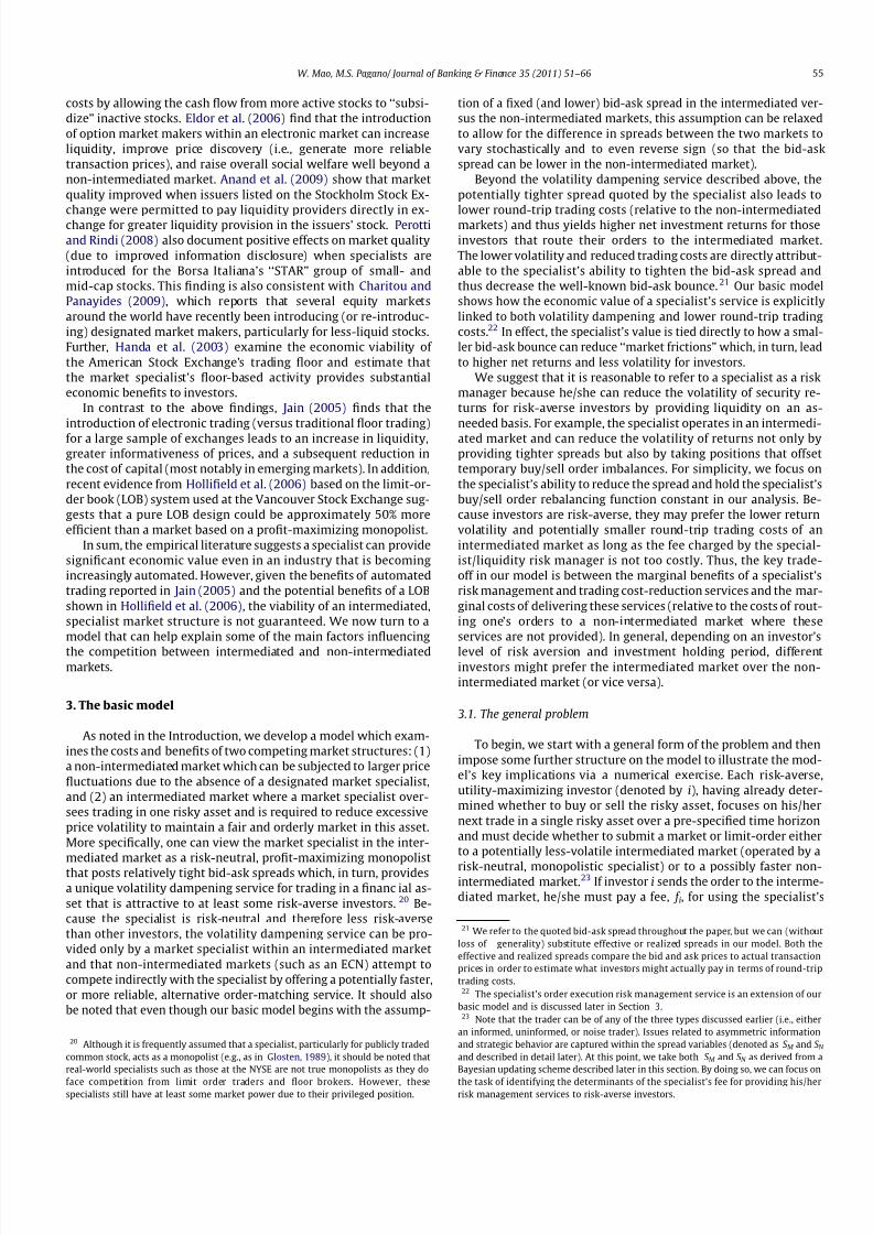
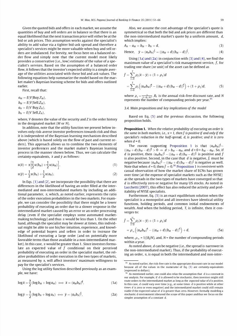
mum willingness to pay. Fig. 1 is a rough sketch of this demand
curve. The results presented in Fig. 1 show the demand curve
and marginal revenue function based on investors with quadratic
utility and differing levels of risk-aversion, as well as a risky asset
with a bid price of $39.975 and an ask price of $40.025 over a 1-
year investment horizon.
Although this figure depicts a specific example of the demand
curve to determine the specialist’s profit-maximizing fee, f *, the
general properties of all concave utility functions can be seen in
this graph. For example, the demand curve in Fig. 1 is nonlinear
and the marginal revenue function does not reach zero (even when
the marginal cost of providing the specialist’s service is zero), thus
illustrating the specialist’s incentive to increase its trading activity.
Since the specialist acts as the monopolist, it will charge a price
where marginal revenue equals marginal cost. If, as shown in
Fig. 1, marginal revenue is greater than zero and marginal cost iszero, then the specialist should charge a price f * based on the mar-
ginal investor who is the least willing to pay and thus the least risk-
averse. Of course, in the case where marginal costs are greater than
zero, the optimal price of f * will be determined where marginal
revenue equals marginal cost. However, since the optimal price is
based on the marginal investor in Fig. 1, for simplicity, the profit-
0
0.01
0.02
0.03
0.04
0.05
0.06
0.07
0.08
0.09
0.1
0 1 2 3 4 5 6
Demand
MR
Q (shares)
i f
f *
0
0.01
0.02
0.03
0.04
0.05
0.06
0.07
0.08
0.09
0.1
Fig. 1. Derivation of demand and marginal revenue functions – quadratic utility.
The graph plots the Demand curve and equilibrium level price, f *, of the specialist’s
risk management service when the marginal revenue (MR) exceeds the marginal
cost (MC) of providing this service (in this graph, we assume for simplicity that
MC = 0). In this case, the equilibrium price equals the maximum willingness to pay
for this service based on the least risk-averse investor’s demand (i.e., f à ¼
f i wherei = the 5th unit of the risky asset).
24 This fee could be in the form of a security-specific specialist commission or an
exchange fee collected from investors by the market center and remitted to the
specialist. The basic point is that this fee should be separate and distinct from the
specialist’s quoted spread because this spread is influenced by other factors (notably,
the costs associated with order processing, inventory management, and asymmetric
information which will be discussed in more detail later).25 Note that the non-intermediated market can also charge a fee like f but, for
simplicity, we assume without loss of generality that this market’s fee is set to zero.
26 For simplicity, and without loss of generality, the non-intermediated market’sprobability is normalized to 50%.
56 W. Mao, M.S. Pagano/ Journal of Banking & Finance 35 (2011) 51–66
7/29/2019 Specialist, Designated Market Makers, Mao_Pagano2011JBF
http://slidepdf.com/reader/full/specialist-designated-market-makers-maopagano2011jbf 7/16
maximizing solution presented here focuses on the least risk-
averse investor.
3.3. Further applications of the basic model
Given that we do not have details on a specific market’s investor
demographics, we pin down the model’s predictions more tightly
by focusing on an even more specific example based on a logarith-mic utility function27:
uð z iÞ ¼ log z i;
where z i is the dollar value of the amount invested in the risky asset
by investor i. Specifically, the degree of absolute risk aversion is
measured by ki ¼ À u00ð z iÞu0ð z iÞ ¼ 1
z i, and it is decreasing with z i (i.e., the
higher the wealth, the less risk-averse the individual becomes).
Also, the log utility function is mainly used for illustration purposes
because, as noted in the earlier example, the key results of the paper
rely solely on the concavity of the utility function. In other words,
the primary assumption necessary to obtain our results is that
investors are risk-averse to varying degrees.
Let S M and S N be the bid-ask spreads for the intermediated mar-
ket (denoted with subscript, M ) and non-intermediated market
(denoted with subscript, N ), respectively:
S M ¼ aM À bM ;
and
S N ¼ aN À bN ;
where aM , bM , aN , and bN stand for the best asking price and best bid
price for the intermediated and non-intermediated markets, respec-
tively, for a particular security that an individual investor is consid-
ering to buy or sell via the market specialist or the ECN-type
market.
A risk-neutral, profit-maximizing specialist in the intermedi-
ated market sets its bid and ask quotes based on the typical Bayes-
ian updating scheme, as described in O’Hara (1997), Bessembinder
et al. (2006), among others. That is, the ask, a, is the expected valueof the security in question, conditioned on observing a buy along
with the history of buying and selling orders thus far. And the
bid, b, is the expected value of the security conditioned on observ-
ing a sell, as well as the current history of orders in the market. 28
Specifically:
AM ¼ E V jBuy; Z M ð Þ;
BM ¼ E V jSell; Z M ð Þ;
AN ¼ E V jBuy; Z N ð Þ;
BN ¼ E V jSell; Z N ð Þ;
where, V denotes the value of the security and Z is the order history
in the designated market (M or N ).
By the dynamics of Bayesian learning, the prices would con-verge to the true value of the security in either the intermediated
or non-intermediated markets. But this convergence will occur at
different rates depending on variations in the level of information
available in the two markets. Thus, we can argue that the
market with more information would have a narrower bid-ask
spread.
As an example, if a specialist provides superior price improve-
ment relative to a non-intermediated market due to more (or bet-
ter) information, then we would expect bM > bN and aN > aM .29 In
this model, we assume that the quote midpoint (QMP ) is the same
for the intermediated market and the non-intermediated market,
i.e., ½(aM + bM ) = ½(aN + bN ), or, aM + bM = aN + bN . This assumption
indicates that neither market has an advantage in terms of price dis-
covery even though, as noted above, one market might be able to of-
fer better price improvement. A potentially important function of the
market specialist as a risk manager is therefore to dampen volatilityby providing competitive bids and offers which reduce the market’s
bid-ask spread relative to a non-intermediated market (so that
S M < S N ). We assume that aN À aM = bM À bN = d, where d is the reduc-
tion of the half-spread by the market specialist. That is, d represents
the price improvement (e.g., in cents per share) a specialist provides
on either the bid or ask sides of the market. And, 2d indicates the
round-trip per-share cost savings associated with using the special-
ist’s services rather than submitting an order to the non-intermedi-
ated market.
For tractability and without loss of generality, we assume a
fixed investment horizon of T -periods for each investor, all of
whom possess the same level of initial wealth and a common per-
sonal utility function, which assumes all investors are risk-
averse.30 In addition, we assume that the price improvements for
both the bids and offers are symmetric (i.e., dbid = dask) and that d
is a constant. However, our results also hold if d is stochastic, as long
as the expected value of d is positive. In fact, the model’s predictions
can still hold even when d is negative (i.e., the non-intermediated
market’s spread is lower than the specialist market’s spread) but this
requires relaxing the assumption of an equal likelihood of order exe-
cution in both markets. Also, we could allow for asymmetry in the
values of d (e.g., dbid – dask) but this additional complication would
still lead to our main results, as detailed later in this section. That
is, ceteris paribus, investors: (a) prefer the intermediated market
when dbid – dask as long as both are greater than zero or (b) prefer
the non-intermediated market when dbid – dask as long as both are
less than zero.
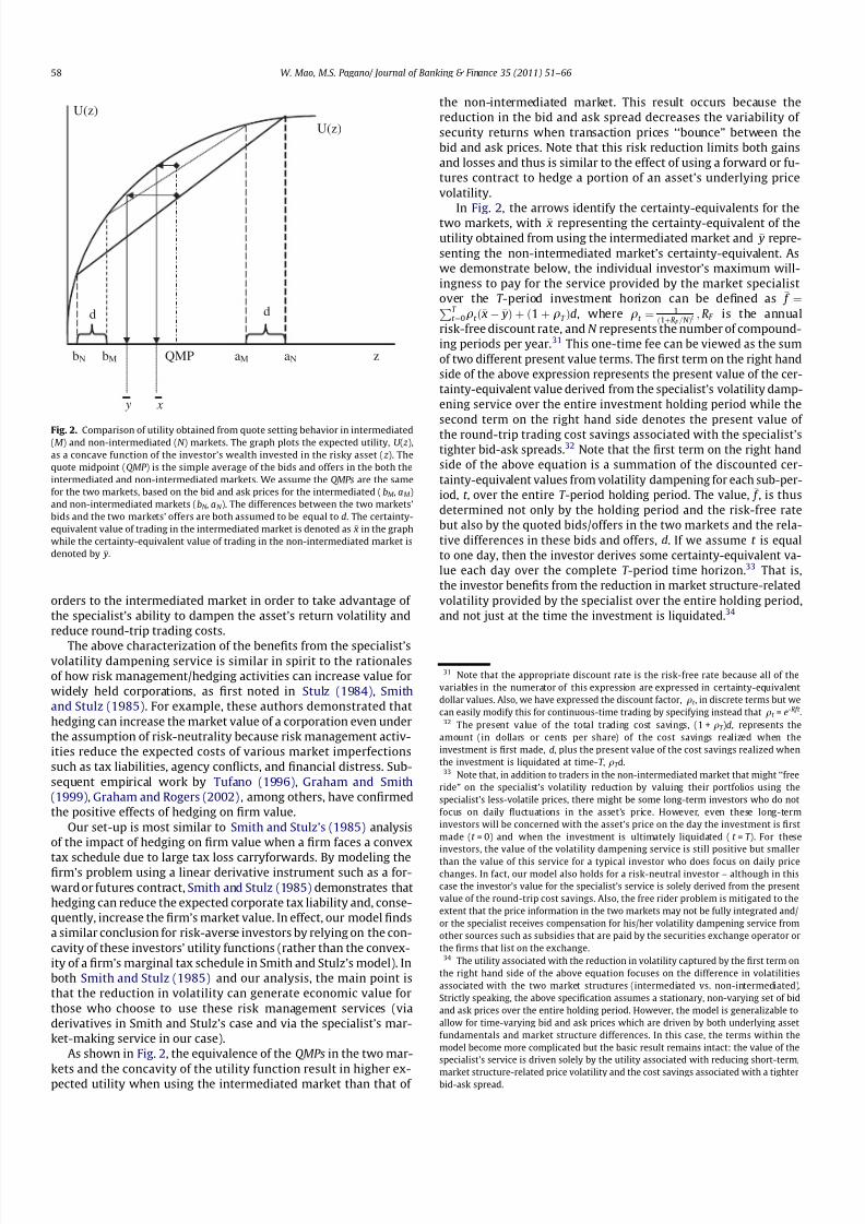
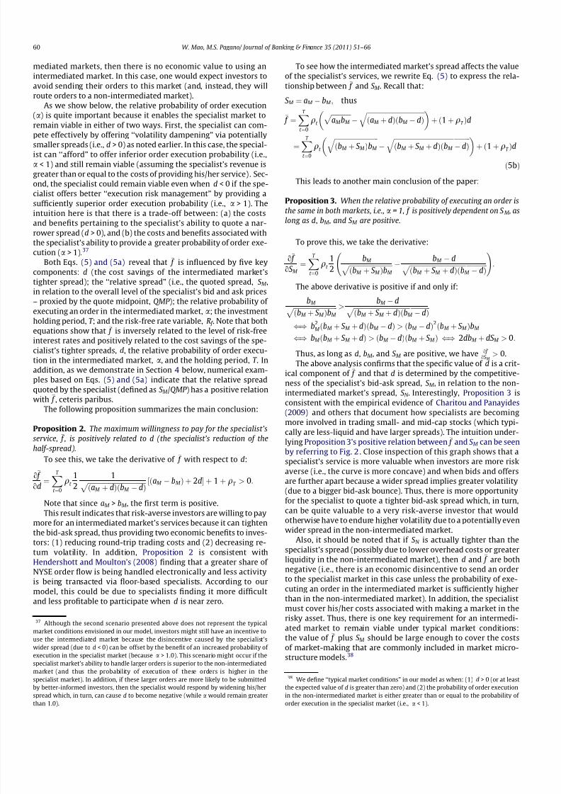
The following graph depicted in Fig. 2 helps capture the essence
of our model. The graph plots the expected utility as a concavefunction of the investor’s wealth invested in the risky asset ( z ).
The quote midpoint (QMP ) is the simple average of the bids and of-
fers in the intermediated markets. As noted above, we assume the
QMPs are the same for the two markets. Because the spread in the
intermediated market is assumed to be smaller while the QMP is
the same in both markets, the certainty-equivalent value of trading
in the intermediated market (denoted as x in the graph) is greater
than the certainty-equivalent value of trading in the non-interme-
diated market (denoted by y). Thus, the certainty-equivalent eco-
nomic value (in dollars) of the specialist’s volatility dampening
service is represented by the difference between x and y in Fig. 2.
In addition to the value of this risk management service, the inves-
tors also save the round-trip trading costs of 2d associated with the
specialist market’s tighter bid-ask spread. That is, in a single peri-od, investors would be willing to pay up to x À y þ 2d to route their
27 Although this section concentrates on a specific utility function, the main results
presented here will still hold as long as investors possess a monotonic, concave utility
function.28 Note that in the non-intermediated market, the best bids and offers are
determined collectively by all traders that submit orders to this market’s limit order
book. These traders will also use a Bayesian updating scheme as noted above for bN
and aN .
29 One possible reason for this type of situation would be if the specialist’s access to
private information about the total order flow (such as reserve orders placed on the
limit order book) provides the specialist with more, or better, information and
therefore can provide him / her with an information advantage relative to a non-
intermediated market. However, it should also be noted that the non-intermediated
market could, in contrast, provide better price improvement via a tighter bid-ask
spread if order processing and other transaction-related costs are sufficiently lower in
this market and thus can offset any potential information advantage of the
intermediated market.30 We could allow each investor to have different time horizons, wealth levels, and
utility functions but the added complications of such assumptions would lead to more
extensive algebra and notation but not change our overall results. Thus, we focus on
the more parsimonious model where all investors are homogeneous. In addition,
within our set-up we can interpret one unit of time, t , to be a discrete period of, say,one day. However, the model can be modified to allow for trading in continuous time.
W. Mao, M.S. Pagano/ Journal of Banking & Finance 35 (2011) 51–66 57
7/29/2019 Specialist, Designated Market Makers, Mao_Pagano2011JBF
http://slidepdf.com/reader/full/specialist-designated-market-makers-maopagano2011jbf 8/16
orders to the intermediated market in order to take advantage of
the specialist’s ability to dampen the asset’s return volatility and
reduce round-trip trading costs.
The above characterization of the benefits from the specialist’svolatility dampening service is similar in spirit to the rationales
of how risk management/hedging activities can increase value for
widely held corporations, as first noted in Stulz (1984), Smith
and Stulz (1985). For example, these authors demonstrated that
hedging can increase the market value of a corporation even under
the assumption of risk-neutrality because risk management activ-
ities reduce the expected costs of various market imperfections
such as tax liabilities, agency conflicts, and financial distress. Sub-
sequent empirical work by Tufano (1996), Graham and Smith
(1999), Graham and Rogers (2002), among others, have confirmed
the positive effects of hedging on firm value.
Our set-up is most similar to Smith and Stulz’s (1985) analysis
of the impact of hedging on firm value when a firm faces a convex
tax schedule due to large tax loss carryforwards. By modeling thefirm’s problem using a linear derivative instrument such as a for-
ward or futures contract, Smith and Stulz (1985) demonstrates that
hedging can reduce the expected corporate tax liability and, conse-
quently, increase the firm’s market value. In effect, our model finds
a similar conclusion for risk-averse investors by relying on the con-
cavity of these investors’ utility functions (rather than the convex-
ity of a firm’s marginal tax schedule in Smith and Stulz’s model). In
both Smith and Stulz (1985) and our analysis, the main point is
that the reduction in volatility can generate economic value for
those who choose to use these risk management services (via
derivatives in Smith and Stulz’s case and via the specialist’s mar-
ket-making service in our case).
As shown in Fig. 2, the equivalence of the QMPs in the two mar-
kets and the concavity of the utility function result in higher ex-pected utility when using the intermediated market than that of
the non-intermediated market. This result occurs because the
reduction in the bid and ask spread decreases the variability of
security returns when transaction prices ‘‘bounce” between the
bid and ask prices. Note that this risk reduction limits both gains
and losses and thus is similar to the effect of using a forward or fu-
tures contract to hedge a portion of an asset’s underlying price
volatility.
In Fig. 2, the arrows identify the certainty-equivalents for thetwo markets, with x representing the certainty-equivalent of the
utility obtained from using the intermediated market and y repre-
senting the non-intermediated market’s certainty-equivalent. As
we demonstrate below, the individual investor’s maximum will-
ingness to pay for the service provided by the market specialist
over the T -period investment horizon can be defined as f ¼PT
t ¼0qt ð x À yÞ þ ð1 þ qT Þd, where qt ¼ 1ð1þRF =N Þt ; RF is the annual
risk-free discount rate, and N represents the number of compound-
ing periods per year.31 This one-time fee can be viewed as the sum
of two different present value terms. The first term on the right hand
side of the above expression represents the present value of the cer-
tainty-equivalent value derived from the specialist’s volatility damp-
ening service over the entire investment holding period while the
second term on the right hand side denotes the present value of
the round-trip trading cost savings associated with the specialist’s
tighter bid-ask spreads.32 Note that the first term on the right hand
side of the above equation is a summation of the discounted cer-
tainty-equivalent values from volatility dampening for each sub-per-
iod, t , over the entire T -period holding period. The value, f , is thus
determined not only by the holding period and the risk-free rate
but also by the quoted bids/offers in the two markets and the rela-
tive differences in these bids and offers, d. If we assume t is equal
to one day, then the investor derives some certainty-equivalent va-
lue each day over the complete T -period time horizon.33 That is,
the investor benefits from the reduction in market structure-related
volatility provided by the specialist over the entire holding period,
and not just at the time the investment is liquidated.34
U(z)
d d
U(z)
zbN bM aM aNQMP
y x
Fig. 2. Comparison of utility obtained from quote setting behavior in intermediated(M ) and non-intermediated (N ) markets. The graph plots the expected utility, U ( z ),
as a concave function of the investor’s wealth invested in the risky asset ( z ). The
quote midpoint (QMP ) is the simple average of the bids and offers in the both the
intermediated and non-intermediated markets. We assume the QMPs are the same
for the two markets, based on the bid and ask prices for the intermediated ( bM , a M )
and non-intermediated markets (bN , a N ). The differences between the two markets’
bids and the two markets’ offers are both assumed to be equal to d. The certainty-
equivalent value of trading in the intermediated market is denoted as x in the graph
while the certainty-equivalent value of trading in the non-intermediated market is
denoted by y.
31 Note that the appropriate discount rate is the risk-free rate because all of the
variables in the numerator of this expression are expressed in certainty-equivalent
dollar values. Also, we have expressed the discount factor, qt , in discrete terms but we
can easily modify this for continuous-time trading by specifying instead that qt = e-Rft .32 The present value of the total trading cost savings, (1 + qT )d, represents the
amount (in dollars or cents per share) of the cost savings realized when the
investment is first made, d, plus the present value of the cost savings realized when
the investment is liquidated at time-T , qT d.33 Note that, in addition to traders in the non-intermediated market that might ‘‘free
ride” on the specialist’s volatility reduction by valuing their portfolios using the
specialist’s less-volatile prices, there might be some long-term investors who do not
focus on daily fluctuations in the asset’s price. However, even these long-term
investors will be concerned with the asset’s price on the day the investment is first
made (t = 0) and when the investment is ultimately liquidated ( t = T ). For these
investors, the value of the volatility dampening service is still positive but smaller
than the value of this service for a typical investor who does focus on daily price
changes. In fact, our model also holds for a risk-neutral investor – although in this
case the investor’s value for the specialist’s service is solely derived from the present
value of the round-trip cost savings. Also, the free rider problem is mitigated to the
extent that the price information in the two markets may not be fully integrated and/
or the specialist receives compensation for his/her volatility dampening service from
other sources such as subsidies that are paid by the securities exchange operator or
the firms that list on the exchange.34 The utility associated with the reduction in volatility captured by the first term on
the right hand side of the above equation focuses on the difference in volatilities
associated with the two market structures (intermediated vs. non-intermediated).
Strictly speaking, the above specification assumes a stationary, non-varying set of bid
and ask prices over the entire holding period. However, the model is generalizable to
allow for time-varying bid and ask prices which are driven by both underlying asset
fundamentals and market structure differences. In this case, the terms within the
model become more complicated but the basic result remains intact: the value of the
specialist’s service is driven solely by the utility associated with reducing short-term,
market structure-related price volatility and the cost savings associated with a tighterbid-ask spread.
58 W. Mao, M.S. Pagano/ Journal of Banking & Finance 35 (2011) 51–66
7/29/2019 Specialist, Designated Market Makers, Mao_Pagano2011JBF
http://slidepdf.com/reader/full/specialist-designated-market-makers-maopagano2011jbf 9/16
Given the quoted bids and offers in each market, we assume the
quantities of buy and sell orders are in balance so that there is an
equal likelihood that the next transaction price will either be at the
bid or ask prices. This assumption works against the specialist’s
ability to add value via a tighter bid-ask spread and therefore a
specialist’s services might be more valuable when buy and sell or-
ders are imbalanced. For brevity, we focus here on a balanced or-
der flow and simply note that the current model most likelyprovides a conservative (i.e., low) estimate of the value of a spe-
cialist’s services. Based on the assumption of a balanced order
flow, it follows that the investor’s expected utility is a simple aver-
age of the utilities associated with these bid and ask values. The
following equations help summarize the model based on the mar-
ket maker’s Bayesian learning scheme for bids and offers outlined
earlier.
First, recall that:
aM ¼ E V jBuy; Z M ð Þ;
bM ¼ E V jSell; Z M ð Þ;
aN ¼ E V jBuy; Z N ð Þ;
bN ¼ E V jSell; Z N ð Þ;
where, V denotes the value of the security and Z is the order history
in the designated market (M or N ).
In addition, note that the utility function we present below in-
volves only risk-averse investor preferences towards risk and thus
it is independent of the Bayesian learning mechanism described
above (which is based solely on the flow of past and current or-
ders). This approach allows us to combine the two elements of
investor preferences and the market maker’s Bayesian learning
process in the manner shown below. Thus, we can calculate the
certainty-equivalents, x and y as follows:
uð xÞ ¼ a1
2uðbM Þ þ
1
2uðaM Þ
; ð1Þ
uð yÞ ¼1
2uðbN Þ þ
1
2uðaN Þ; ð2Þ
In Eqs. (1) and (2), we incorporate the possibility that there are
differences in the likelihood of having an order filled at the inter-
mediated and non-intermediated markets by including an addi-
tional parameter, a, which, as noted earlier, represents the ratio
of the order execution probabilities in the two markets. For exam-
ple, we can consider the possibility that there might be a lower
probability of executing an order due to a slower response in the
intermediated market caused by an error or an order processing
delay (even if the specialist employs some automated market-
making technology) and thus a would be less than 1. On the other
hand, although the specialist may be slower at times, this individ-
ual might be able to use his/her intuition, experience, and knowl-
edge of potential buyers and sellers in order to increase the
likelihood of executing a large order (and on potentially morefavorable terms than those available in a non-intermediated mar-
ket). In this case, a would be greater than 1. Since investors formu-
late an expected value of f conditional on their perceived
probability of executing an order in the specialist market, the rel-
ative probabilities of order execution in the two types of markets,
as measured by a, will affect investors’ maximum willingness to
pay for the specialist’s services.
Using the log utility function described previously as an exam-
ple, we have:
log x ¼a
2log bM þ log aM ð Þ () x ¼ aM bM ð Þ
a2; ð1aÞ
log y ¼1
2 log bN þ log aN ð Þ () y ¼ aN bN ð Þ1
2; ð2aÞ
Also, we assume the cost advantage of the specialist’s quote is
symmetrical so that both the bid and ask prices are different than
the non-intermediated market’s quote by a uniform amount, d,
which implies:
AN À aM ¼ bM À bN ¼ d; ð3Þ
Hence; y ¼ aN bN ð Þ12 ¼ aM þ dð Þ bM À dð Þð Þ
12; ð4Þ
Using (1a) and (2a) in conjunction with (3) and (4), we find themaximum value of a specialist’s risk management service, f , for
trading one share (or unit) of the asset can be defined as
f ¼XT
t ¼0
qt x À yð Þ þ 1 þ qT ð Þd
¼XT
t ¼0
qt aM bM ð Þa2 À aM þ dð Þ bM À dð Þð Þ
12
þ 1 þ qT ð Þd; ð5Þ
where qt ¼ 1ð1þRF =N Þt ;RF is the annual risk-free discount rate, and N
represents the number of compounding periods per year.35
3.4. Main propositions and key implications of the model
Based on Eq. (5) and the previous discussion, the followingproposition holds.
Proposition 1. When the relative probability of executing an order is
the same in both markets, i.e., a = 1, then f is positive if and only if the
specialist’s reduction in the half-spread, d, is positive; and it is zero
when d = 0.
The reason supporting Proposition 1 is that ðaM bM Þ12À
ððaM þ dÞðbM À dÞÞ12 > 0 ) d > bM À aM , and d > 0 > bM À aM . So, if
d is positive, then ðaM bM Þ12 À ððaM þ dÞðbM À dÞÞ1
2 is positive and f
is also positive. Second, in the case that d is negative, f i must be
negative because ðaM bM Þ12 À ððaM þ dÞðbM À dÞÞ1
2 is negative as well.
Note that when d = 0, then f ¼ 0.36 Proposition 1 is consistent with
casual observation of how the market share of ECNs has grown
over time (at the expense of specialist markets such as the NYSE)as the spreads in the two types of markets have converged so that
d is effectively zero or negative for many US stocks. As noted in
Lucchetti (2007), this effect has also reduced the activity and prof-
itability of NYSE specialists.
Furthermore, Eq. (5) is an exact equilibrium solution when the
specialist is a monopolist and all investors have identical utility
functions, holding periods, and common initial endowments of
wealth. And when the holding period, T , is infinite, then it con-
verges to:
f ¼X1
t ¼0
qt x À yð Þ þ 1 þ qT ð Þd
¼ q1 aM bM ð Þa2 À aM þ dð Þ bM À dð Þð Þ
12
þ d; ð5aÞ
where, q1 = 1/(R f /N ), and, N = the number of compounding periods
within a year.
As noted above, d can be negative (i.e., the spread is narrower in
the non-intermediated market). Thus, if the probability of execut-
ing an order, a, is equal in both the intermediated and non-inter-
35 As noted earlier, the risk-free rate is the appropriate discount rate in our model
because all of the values in the numerator of Eq. (5) are certainty-equivalents
(expressed in dollars).36 As mentioned earlier, one could also relax the assumption that d is a constant in
our analysis. For example, if d is allowed to be stochastic, then investors might still
route orders to the intermediated market as long as the expected value of d is positive.
In this case, d could vary over time (e.g., at some times d is positive while at other
times d is zero or even negative) and the intermediated market could still remain
viable if the expected value of d is greater than zero. However, formally modeling a
stochastic d environment isbeyond the scope of this paper andthus we focus on thesimpler assumption of a constant d.
W. Mao, M.S. Pagano/ Journal of Banking & Finance 35 (2011) 51–66 59
7/29/2019 Specialist, Designated Market Makers, Mao_Pagano2011JBF
http://slidepdf.com/reader/full/specialist-designated-market-makers-maopagano2011jbf 10/16
mediated markets, then there is no economic value to using an
intermediated market. In this case, one would expect investors to
avoid sending their orders to this market (and, instead, they will
route orders to a non-intermediated market).
As we show below, the relative probability of order execution
(a) is quite important because it enables the specialist market to
remain viable in either of two ways. First, the specialist can com-
pete effectively by offering ‘‘volatility dampening” via potentiallysmaller spreads (i.e., d > 0) as noted earlier. In this case, the special-
ist can ‘‘afford” to offer inferior order execution probability (i.e.,
a < 1) and still remain viable (assuming the specialist’s revenue is
greater than or equal to the costs of providing his/her service). Sec-
ond, the specialist could remain viable even when d < 0 if the spe-
cialist offers better ‘‘execution risk management” by providing a
sufficiently superior order execution probability (i.e., a > 1). The
intuition here is that there is a trade-off between: (a) the costs
and benefits pertaining to the specialist’s ability to quote a nar-
rower spread (d > 0), and (b) the costs and benefits associated with
the specialist’s ability to provide a greater probability of order exe-
cution (a > 1).37
Both Eqs. (5) and (5a) reveal that f is influenced by five key
components: d (the cost savings of the intermediated market’s
tighter spread); the ‘‘relative spread” (i.e., the quoted spread, S M ,
in relation to the overall level of the specialist’s bid and ask prices
– proxied by the quote midpoint, QMP ); the relative probability of
executing an order in the intermediated market, a; the investment
holding period, T ; and the risk-free rate variable, R f . Note that both
equations show that f is inversely related to the level of risk-free
interest rates and positively related to the cost savings of the spe-
cialist’s tighter spreads, d, the relative probability of order execu-
tion in the intermediated market, a, and the holding period, T . In
addition, as we demonstrate in Section 4 below, numerical exam-
ples based on Eqs. (5) and (5a) indicate that the relative spread
quoted by the specialist (defined as S M /QMP ) has a positive relation
with f , ceteris paribus.
The following proposition summarizes the main conclusion:
Proposition 2. The maximum willingness to pay for the specialist’s
service, f , is positively related to d (the specialist’s reduction of the
half-spread).
To see this, we take the derivative of f with respect to d:
o f
od¼XT
t ¼0
qt
1
2
1 ffiffiffiffiffiffiffiffiffiffiffiffiffiffiffiffiffiffiffiffiffiffiffiffiffiffiffiffiffiffiffiffiffiffiffiffiaM þ dð Þ bM À dð Þ
p aM À bM ð Þ þ 2d½ þ 1 þ qT > 0:
Note that since aM > bM , the first term is positive.
This result indicates that risk-averse investors are willing to pay
more for an intermediated market’s services because it can tighten
the bid-ask spread, thus providing two economic benefits to inves-
tors: (1) reducing round-trip trading costs and (2) decreasing re-
turn volatility. In addition, Proposition 2 is consistent with
Hendershott and Moulton’s (2008) finding that a greater share of
NYSE order flow is being handled electronically and less activity
is being transacted via floor-based specialists. According to our
model, this could be due to specialists finding it more difficult
and less profitable to participate when d is near zero.
To see how the intermediated market’s spread affects the value
of the specialist’s services, we rewrite Eq. (5) to express the rela-
tionship between f and S M . Recall that:
S M ¼ aM À bM ; thus
f ¼XT
t ¼0
qt
ffiffiffiffiffiffiffiffiffiffiffiffiaM bM
p À
ffiffiffiffiffiffiffiffiffiffiffiffiffiffiffiffiffiffiffiffiffiffiffiffiffiffiffiffiffiffiffiffiffiffiffiffiaM þ dð Þ bM À dð Þ
q þ 1 þqT ð Þd
¼XT
t ¼0
qt
ffiffiffiffiffiffiffiffiffiffiffiffiffiffiffiffiffiffiffiffiffiffiffiffiffiffiffibM þ S M ð ÞbM
q À
ffiffiffiffiffiffiffiffiffiffiffiffiffiffiffiffiffiffiffiffiffiffiffiffiffiffiffiffiffiffiffiffiffiffiffiffiffi ffiffiffiffiffiffiffiffiffiffibM þ S M þ dð Þ bM À dð Þ
q þ 1 þqT ð Þd
ð5bÞ
This leads to another main conclusion of the paper:
Proposition 3. When the relative probability of executing an order is
the same in both markets, i.e., a = 1, f is positively dependent on S M , as
long as d, bM , and S M are positive.
To prove this, we take the derivative:
o f
oS M
¼
XT
t ¼0
qt
1
2
bM
ffiffiffiffiffiffiffiffiffiffiffiffiffiffiffiffiffiffiffiffiffiffiffiffiffiffiffibM þ S M ð ÞbM p À
bM À d
ffiffiffiffiffiffiffiffiffiffiffiffiffiffiffiffiffiffiffiffiffiffiffiffiffiffiffiffiffiffiffiffiffiffiffi ffiffiffiffiffiffiffiffiffiffiffiffiffibM þ S M þ dð Þ bM À dð Þp !
:
The above derivative is positive if and only if:
bM ffiffiffiffiffiffiffiffiffiffiffiffiffiffiffiffiffiffiffiffiffiffiffiffiffiffiffibM þ S M ð ÞbM
p >bM À d ffiffiffiffiffiffiffiffiffiffiffiffiffiffiffiffiffiffiffiffiffiffiffiffiffiffiffiffiffiffiffiffiffiffiffi ffiffiffiffiffiffiffiffiffiffiffiffi
bM þ S M þ dð Þ bM À dð Þp
() b2M bM þ S M þ dð Þ bM À dð Þ > bM À dð Þ
2bM þ S M ð ÞbM
() bM bM þ S M þ dð Þ > bM À dð Þ bM þ S M ð Þ () 2dbM þ dS M > 0:
Thus, as long as d, bM , and S M are positive, we have o f oS M
> 0.
The above analysis confirms that the specific value of d is a crit-
ical component of f and that d is determined by the competitive-
ness of the specialist’s bid-ask spread, S M , in relation to the non-
intermediated market’s spread, S N . Interestingly, Proposition 3 is
consistent with the empirical evidence of Charitou and Panayides
(2009) and others that document how specialists are becoming
more involved in trading small- and mid-cap stocks (which typi-
cally are less-liquid and have larger spreads). The intuition under-
lying Proposition 3’s positive relation between f and S M can be seen
by referring to Fig. 2. Close inspection of this graph shows that a
specialist’s service is more valuable when investors are more risk
averse (i.e., the curve is more concave) and when bids and offers
are further apart because a wider spread implies greater volatility
(due to a bigger bid-ask bounce). Thus, there is more opportunity
for the specialist to quote a tighter bid-ask spread which, in turn,
can be quite valuable to a very risk-averse investor that would
otherwise have to endure higher volatility due to a potentially even
wider spread in the non-intermediated market.
Also, it should be noted that if S N is actually tighter than the
specialist’s spread (possibly due to lower overhead costs or greater
liquidity in the non-intermediated market), then d and f are bothnegative (i.e., there is an economic disincentive to send an order
to the specialist market in this case unless the probability of exe-
cuting an order in the intermediated market is sufficiently higher
than in the non-intermediated market). In addition, the specialist
must cover his/her costs associated with making a market in the
risky asset. Thus, there is one key requirement for an intermedi-
ated market to remain viable under typical market conditions:
the value of f plus S M should be large enough to cover the costs
of market-making that are commonly included in market micro-
structure models.38
37 Although the second scenario presented above does not represent the typical
market conditions envisioned in our model, investors might still have an incentive to
use the intermediated market because the disincentive caused by the specialist’s
wider spread (due to d < 0) can be offset by the benefit of an increased probability of
execution in the specialist market (because a > 1.0). This scenario might occur if the
specialist market’s ability to handle larger orders is superior to the non-intermediated
market (and thus the probability of execution of these orders is higher in the
specialist market). In addition, if these larger orders are more likely to be submitted
by better-informed investors, then the specialist would respond by widening his/her
spread which, in turn, can cause d to become negative (while a would remain greaterthan 1.0).
38 We define ‘‘typical market conditions” in our model as when: (1) d > 0 (or at least
the expected value of d is greater than zero) and (2) the probability of order execution
in the non-intermediated market is either greater than or equal to the probability of order execution in the specialist market (i.e., a < 1).
60 W. Mao, M.S. Pagano/ Journal of Banking & Finance 35 (2011) 51–66
7/29/2019 Specialist, Designated Market Makers, Mao_Pagano2011JBF
http://slidepdf.com/reader/full/specialist-designated-market-makers-maopagano2011jbf 11/16
That is, f plus S M represents the total specialist revenue from
trading one unit (or share) of the risky asset. Via the assumption
that d is a constant, our model suggests that the way specialists
are compensated for their services should include a fixed compo-
nent (the upper bound of which is f ) and a potentially variable
component (S M ) which can adjust dynamically with market condi-
tions related to the underlying asset.39 Overall, for the specialist to
stay viable, the sum of
f and S M must be greater than or equal to thespecialist’s order processing costs, inventory holding costs, and any
costs associated with trading against more-informed traders. There-
fore, our model is indirectly related to the existing literature of Kyle
(1985), Glosten and Milgrom (1985), Glosten and Harris (1988),
Glosten (1989), and others because these strategic trader-based
‘‘spread” models provide a floor on how much the specialist can
charge investors and still remain viable. More formally, we can state
this relationship as follows:
f þ S M P Total Trading Costs ðper shareÞ ¼ AC
¼ g ðINV ; AI ;KL;Q Þ > 0: ð6Þ
The total trading costs (per share) should equal the expected
average cost, AC , associated with the following four key
components:
INV , the cost of holding shares in the underlying security in
inventory to assist in maintaining a fair and orderly market.
AI , the cost of trading with informed traders that know more
than the market specialist (i.e., an adverse selection cost caused
by information asymmetries between traders).
KL, the cost of physical capital and the specialist’s labor associ-
ated with providing the market-making service (e.g., the cost of
computers, software, regulatory compliance, salaries/wages),
and
Q , the quantity of shares traded by the specialist during the
trading period.
From Eq. (6), we can see that the viability of the intermediatedmarket depends on the specialist’s ability to charge enough to
cover the above costs that have been identified by previous theo-
retical and empirical research. The first three variables on the
right hand side of (6) are positively related to total trading costs
(per share) while trading volume (Q ) is inversely related to AC .
Interestingly, if f plus S M cannot cover these costs, then the spe-
cialist market might not be economically viable and we would ex-
pect only a non-intermediated market to exist. Eq. (6) also
illustrates how changes in trading volume as well as the costs
of order processing, inventory management, and asymmetric
information can be incorporated within our model. Our model
thus shows that a specialist must generate sufficient value via
its volatility dampening and trading cost reduction services in or-
der to justify the intermediated market’s viability. In contrast to
the existing literature, the specialist can no longer assume he/
she can set the bid-ask spread to recover the costs associated with
asymmetric information, inventory management, and order pro-
cessing. In a world with a non-intermediated market alternative,
the specialist must ensure he/she adds sufficient value to cover
these market-making costs.
In the remainder of the theoretical analysis, we assume that f
plus S M is greater than or equal to this floor level, AC , and that AC
is constant.40 Lastly, we cannot examine the relationship between
the maximum willingness to pay for the specialist service, f , and
the degree of investor risk aversion using the log utility function.
However, we do examine this issue with the quadratic utility func-
tion in the Appendix A.
Proposition 4. The maximum willingness to pay for the specialist’s
service, f , is positively related to a, the relative probability of execution
in the intermediated market.
To see this, we show that:o f
oa¼XT
t ¼0
qt aM bM ð Þa=2
log aM bM ð Þ1=2
h i
¼XT
t ¼0
qt
1
2aM bM ð Þ
a=2log aM bM ð Þ > 0:
Note that the above is true if and only if aM bM > 1.41
As the relative probability of execution in the intermediated
market increases (a rises), then the risk of non-execution in the
intermediated market decreases and, in turn, raises the trader’s
willingness to pay for the specialist’s risk management service. 42
However, an investor wishing to trade a very large block of stock
might perceive a very small probability of executing this large order
in the intermediated market (e.g., due to specialist capital con-
straints, fears of information leakage, front-running, etc.). For this
investor, a might be close to zero and thus, according to (5b), the tra-
der might find that f is negative. In this case, there can be an eco-
nomic disincentive to send the large order to the intermediated
market and he/she might therefore choose to route the order to
the non-intermediated market. Consistent with Proposition 4, the
continued growth of non-intermediated ATS-type markets such as
ITG’s Posit, Liquidnet, and Pipeline in recent years suggests that
institutional investors might perceive a to be relatively low in the
traditional US equity market centers for large orders (and thus these
investors opt to route many of their 10,000 + share orders away from
the intermediated markets).43 In sum, the above analysis suggests
that a can be an important determinant of f beyond the four vari-
ables already discussed above (i.e., d, T, S M /QMP , and R f ).
4. Numerical application of the basic model
To provide further insight into the model’s implications, we re-
port in Table 1 some numerical examples for three hypothetical
securities with varying levels of (1) quote midpoints (QMP ), (2)
half-spreads (i.e., half of the bid-ask spread), and (3) cost advanta-
ges over non-intermediated markets (d). The % Spread values in Ta-
ble 1 denote the quoted spread in the intermediated market for
each of the three securities as a percentage of the respective quote
midpoints (i.e., % Spread = S M /QMP ). As can be seen from Table 1,
the three securities’ QMPs range from $10 to $100 per unit while
the relative quoted spreads vary from 2 to 100 basis points. This
range in QMP and relative spreads is meant to capture the typical
cross-sectional variation in current US equities markets causedby differences in liquidity. The value of d also varies from 1 cent
39 For example, even when S M = 0, both d and f can still be positive; as can be seen
by setting S M = 0 within Eq. (5b).40 We hold AC constant in our analysis but this assumption can be relaxed if one
wishes to explore the impact of AC’s variables on
f . Since this would be beyond thescope of this paper, we leave this issue as a possible avenue for future research.
41 This condition is easily met as long as the asset’s bid and offer prices are above
$1.00 (which is the case for all US stocks except those referred to as ‘‘penny” stocks).42 An increase in a might be due to increased automation and faster response time
by the specialist via the introduction of specialist-specific proprietary, automated
trading algorithms (such as those being developed by US market centers such as the
New York Stock Exchange).43 In addition, these institutional traders have increasingly ‘‘sliced and diced” their
large orders into several smaller orders and submitted them sequentially to an
intermediated market in order to minimize adverse market impact and lessen
information ‘‘leakage” about these orders. In effect, this slicing and dicing activity
could be viewed as another way for large traders to realize a higher a collectively, for
their set of smaller orders (whereas the expected a for one large order might be quite
low). This behavior also suggests that a can be very different for various types of
investors (and even different types of orders for the same investor might havediffering a values). This possibility is left for future research.
W. Mao, M.S. Pagano/ Journal of Banking & Finance 35 (2011) 51–66 61
7/29/2019 Specialist, Designated Market Makers, Mao_Pagano2011JBF
http://slidepdf.com/reader/full/specialist-designated-market-makers-maopagano2011jbf 12/16
to 10 cents in order to provide an economically meaningful differ-
ence in the costs of trading on the intermediated market vis-à-vis
the non-intermediated market. All results are based on a fixed, an-
nual risk-free discount rate of 5% (compounded daily) and a is con-
stant at 1.
The values reported for the three columns under theholding per-
iod heading contain estimates based on 1-day, 1-year, and infinite
investment holding periods. Panel A of Table 1 provides estimatesof the maximum willingness to pay for the specialist’s services, f ,
while Panel B reports the proportion of these f estimates which
are directly attributable to the economic value of the specialist’s
volatility dampening service.
As can be seen from the f estimates of Table 1, there is substan-
tial variation in the value of the specialist’s services due to differ-
ences in holding periods (T in our model), the intermediated
market’s relative spread (% Spread), and the value of d. Table 1
demonstrates that the value of f is driven almost entirely by the
trading cost savings related to d when the time horizon is very
short (i.e., when T = 1 day). In effect, f is only slightly above 2d
for all three securities when T = 1 day. Further, Panel B shows that
the value of the specialist’s risk reduction service is less than 1% of
the overall value of f for all three assets when investors have a 1-
day holding period.
So, when T is short, the risk management service is not very
valuable for any combination of QMP , bid-ask spread, and d. This
is not surprising because the value of the specialist’s volatility
dampening should not be very high if this risk management ser-
vice is only ‘‘used” by the investor for a single day. That is, the va-
lue of risk management in this case is low because an investor’s
exposure to the asset’s price volatility is also very low (because
prices do not usually fluctuate dramatically over the course of
one day). However, the results change dramatically when the
holding period is extended to 1 year or an infinite time horizon.
For a 1-year holding period, f varies from 2 to 23 cents and this
range increases to 2.1 cents – $2.787 for the infinite horizon. As ex-
pected, the value of the specialist’s risk reduction activity increases
as a percentage of the f estimates when the time horizon is ex-tended. For example, risk reduction now accounts for over half
of the 1-year f estimate for the security with a QMP of $10 (i.e.,
57.8%). In addition, the specialist’s volatility dampening service
represents the majority of the value associated with f when these
estimates are computed over an infinite time horizon (ranging
from 52.3% to 98.2% for the $100- and $10-QMP securities,
respectively).
In terms of the intermediated market’s spread, S M , and the as-
set’s QMP , we find that f is more valuable when the % Spread is
higher. As Panel A of Table 1 shows, the asset with a $10 QMP
has a higher % Spread of 100 basis points and also reports f esti-
mates that are further above 2d than the two other assets with
lower % Spread values. In contrast, f does not vary much for the
security with the lowest relative spread (i.e.,
f for the $100 QMPsecurity is between 2.0 and 2.1 cents for all holding periods in Ta-
ble 1). So, when d and S M are held constant, lower levels of QMP re-
sult in larger f estimates, while higher levels of QMP lead to smaller f estimates. Thus, the overall level of an asset’s price and its rela-
tion to the intermediated market’s spread can also have a strong
influence on f , with less-liquid stocks (i.e., those with a high %Spread) having larger values for f .
In sum, the numerical examples displayed in Table 1 confirm
that tighter spreads in the intermediated market (as measured
by d) can be a critical component in determining the value of the
specialist’s service, f . In addition, the examples illustrate how the
investor’s holding period, T , affects the relative contribution of
the specialist’s two key services: (1) risk management activity
and (2) the round-trip trading cost savings associated with a tigh-ter spread. For very short holding periods such as one day, the spe-
cialist’s value is determined mostly by the round-trip cost savings
associated with tighter spreads (especially for more-liquid assets
with low relative spreads) while progressively longer holding peri-
ods shift the total value of the specialist’s service more towards the
volatility dampening service. The numerical examples suggest that
d, % Spread, and T are important determinants of investor’s willing-
ness to pay for the specialist’s volatility dampening service.44 As
noted earlier, this risk management service also has some qualitiesof a public good. Therefore, even though the specialist’s risk reduc-
tion activity can have a relatively small value for, say, a short-term
individual investor, this service can have a large market-wide value
when cumulated across all investors. Thus, even when the holding
period of the average investor is short, the specialist’s risk reduction
activity can provide a substantial benefit to the overall market and
society in general.
5. Evidence from simulations and Rule 605 order execution data
We provide further evidence about our model’s implications via
numerical simulations as well as some empirical tests based on
SEC Rule 605’s order execution information in Fig. 3 and Table 2,
respectively. For the numerical simulation, we use the specialist’srisk management pricing equation for f based on the quadratic
utility function reported in the Appendix A. Accordingly, we use
Eq. (5c) from the Appendix A to simulate the maximum willingness
to pay for the specialist’s services when both the investor’s holding
period (T ) and his/her risk aversion (c) are allowed to vary over a 1
to 250-trading day horizon.
Fig. 3 displays the f on the vertical axis and the investor’s hold-
ing period (T ) and risk aversion (c) on the x- and z -axes. In this
simulation, we use a specialist’s bid price of $39.975 and an ask
price of $40.025, with d equal to 2.5 cents per trading unit. We
then vary the holding period from 1 to 250 trading days while also
varying c from .005 to .025. The graph shows that the investor’s
willingness to pay for the intermediated market’s services is posi-
tively and nonlinearly related to both T and c. In particular, when
risk aversion is low (e.g., .005), the simulated value of f remains
fairly small and constant at just above 5 cents per trading unit—
even as the holding period is extended to a full year. Conversely,
when risk aversion is high (.025), f increases in a slightly nonlinear
manner over longer holding periods. Interestingly, f grows expo-
nentially from around 5 cents to nearly 19 cents per trading unit
when both the holding period and risk aversion increase. In sum,
this graph illustrates the importance that investor demographics
such as investment horizon and risk aversion jointly play in deter-
mining the equilibrium price for the specialist’s risk management
services.
Going beyond the simulation results noted above, we compare
in Table 2 the SEC Rule 605 order execution statistics of the NYSE
floor-based system to those of NYSE’s ARCA ECN system. This com-
parison provides a useful test of our model’s predictions becauseboth trading venues can trade NYSE-listed stocks and the main dif-
ference between the two venues is the structure of the markets (as
noted in the Introduction, NYSE’s floor is an intermediated market
while ARCA’s ECN is an electronic non-intermediated market). To
conserve space, we focus on the order execution statistics for small
market orders (100–499 shares) during two periods: June 2006 and
44 Two caveats should also be noted here. First, the numerical examples in Table 1
all assume the relative probability of execution in the intermediated market, a, is
100%. Clearly, if this assumption is relaxed, then this additional variable will play an
important role in determining the value of f . Second, our numerical examples also
assume all investors have the same level of wealth, utility function, and time horizon.
Thus, these assumptions need to be relaxed if one wanted to assess the value of f in a
real-world setting. Since the numerical examples are meant solely to demonstrate the
sensitivity of our estimates to various levels of d, T , and QMP , we do not pursue therelaxation of the ‘‘representative investor” assumption.
62 W. Mao, M.S. Pagano/ Journal of Banking & Finance 35 (2011) 51–66
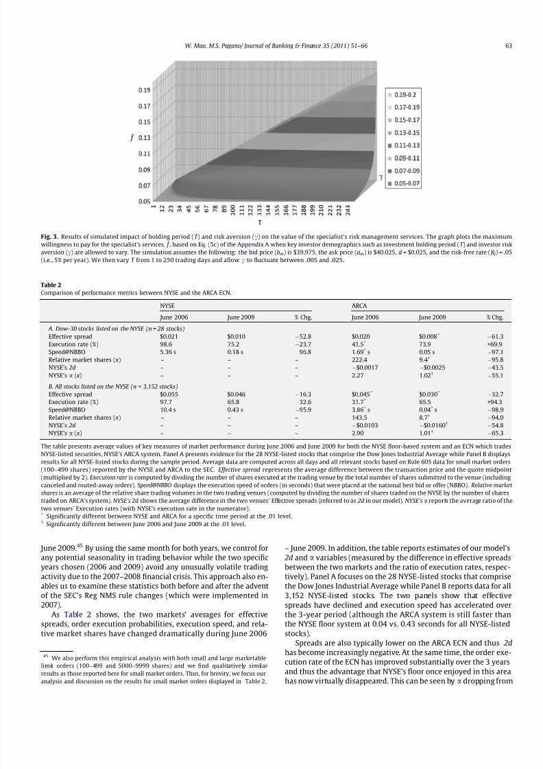
7/29/2019 Specialist, Designated Market Makers, Mao_Pagano2011JBF
http://slidepdf.com/reader/full/specialist-designated-market-makers-maopagano2011jbf 13/16
June 2009.45 By using the same month for both years, we control for
any potential seasonality in trading behavior while the two specific
years chosen (2006 and 2009) avoid any unusually volatile trading
activity due to the 2007–2008 financial crisis. This approach also en-
ables us to examine these statistics both before and after the advent
of the SEC’s Reg NMS rule changes (which were implemented in
2007).
As Table 2 shows, the two markets’ averages for effective
spreads, order execution probabilities, execution speed, and rela-
tive market shares have changed dramatically during June 2006
– June 2009. In addition, the table reports estimates of our model’s
2d and a variables (measured by the difference in effective spreads
between the two markets and the ratio of execution rates, respec-
tively). Panel A focuses on the 28 NYSE-listed stocks that comprise
the Dow Jones Industrial Average while Panel B reports data for all
3,152 NYSE-listed stocks. The two panels show that effective
spreads have declined and execution speed has accelerated over
the 3-year period (although the ARCA system is still faster than
the NYSE floor system at 0.04 vs. 0.43 seconds for all NYSE-listed
stocks).
Spreads are also typically lower on the ARCA ECN and thus 2d
has become increasingly negative. At the same time, the order exe-
cution rate of the ECN has improved substantially over the 3 years
and thus the advantage that NYSE’s floor once enjoyed in this areahas now virtually disappeared. This can be seen by a dropping from
Fig. 3. Results of simulated impact of holding period (T ) and risk aversion (c) on the value of the specialist’s risk management services. The graph plots the maximum
willingness to pay for the specialist’s services, f , based on Eq. (5c) of the Appendix A when key investor demographics such as investment holding period ( T ) and investor risk
aversion (c) are allowed to vary. The simulation assumes the following: the bid price (bm) is $39.975, the ask price (am) is $40.025, d = $0.025, and the risk-free rate (R f ) = .05
(i.e., 5% per year). We then vary T from 1 to 250 trading days and allow c to fluctuate between .005 and .025.
Table 2
Comparison of performance metrics between NYSE and the ARCA ECN.
NYSE ARCA
June 2006 June 2009 % Chg. June 2006 June 2009 % Chg.
A. Dow-30 stocks listed on the NYSE (n = 28 stocks)
Effective spread $0.021 $0.010 À52.8 $0.020 $0.008* À61.3
Execution rate (%) 98.6 75.2 À23.7 43.5* 73.9 +69.9
Speed@NBBO 5.36 s 0.18 s À96.8 1.69* s 0.05 s À97.1
Relative market shares ( x) – – – 222.4 9.4 À95.8
NYSE’s 2d – – – À$0.0017 À$0.0025 À43.5
NYSE’s a ( x) – – – 2.27 1.02 À55.1
B. All stocks listed on the NYSE (n = 3,152 stocks)
Effective spread $0.055 $0.046 À16.3 $0.045* $0.030* À32.7
Execution rate (%) 97.7 65.8 À32.6 33.7*
65.5 +94.3Speed@NBBO 10.4 s 0.43 s À95.9 3.86* s 0.04* s À98.9
Relative market shares ( x) – – – 143.5 8.7 À94.0
NYSE’s 2d – – – À$0.0103 À$0.0160 À54.8
NYSE’s a ( x) – – – 2.90 1.01 À65.3
The table presents average values of key measures of market performance during June 2006 and June 2009 for both the NYSE floor-based system and an ECN which trades
NYSE-listed securities, NYSE’s ARCA system. Panel A presents evidence for the 28 NYSE-listed stocks that comprise the Dow Jones Industrial Average while Panel B displays
results for all NYSE-listed stocks during the sample period. Average data are computed across all days and all relevant stocks based on Rule 605 data for small market orders
(100–499 shares) reported by the NYSE and ARCA to the SEC. Effective spread represents the average difference between the transaction price and the quote midpoint
(multiplied by 2). Execution rate is computed by dividing the number of shares executed at the trading venue by the total number of shares submitted to the venue (including
canceled and routed-away orders). Speed@NBBO displays the execution speed of orders (in seconds) that were placed at the national best bid or offer (NBBO). Relative market
shares is an average of the relative share trading volumes in the two trading venues (computed by dividing the number of shares traded on the NYSE by the number of shares
traded on ARCA’s system). NYSE’s 2d shows the average difference in the two venues’ Effective spreads (referred to as 2d in our model). NYSE’s a reports the average ratio of the
two venues’ Execution rates (with NYSE’s execution rate in the numerator).* Significantly different between NYSE and ARCA for a specific time period at the .01 level. Significantly different between June 2006 and June 2009 at the .01 level.
45 We also perform this empirical analysis with both small and large marketable
limit orders (100–499 and 5000–9999 shares) and we find qualitatively similar
results as those reported here for small market orders. Thus, for brevity, we focus ouranalysis and discussion on the results for small market orders displayed in Table 2.
W. Mao, M.S. Pagano/ Journal of Banking & Finance 35 (2011) 51–66 63
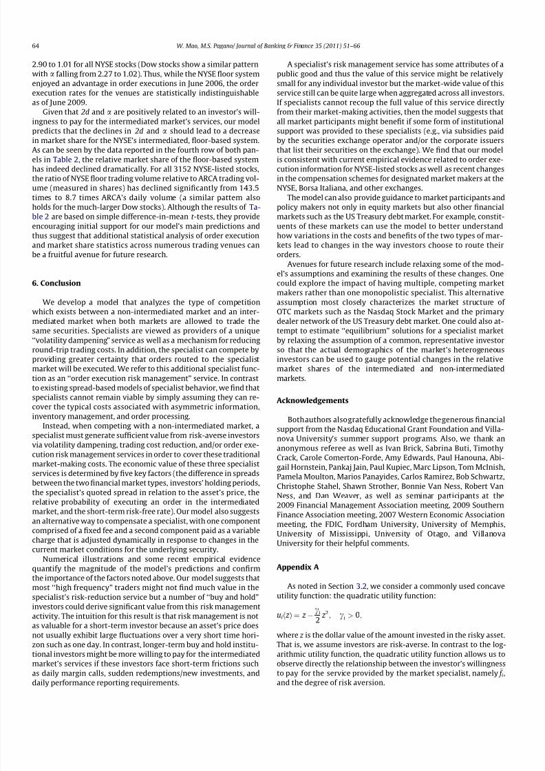
7/29/2019 Specialist, Designated Market Makers, Mao_Pagano2011JBF
http://slidepdf.com/reader/full/specialist-designated-market-makers-maopagano2011jbf 14/16
2.90 to 1.01 for all NYSE stocks (Dow stocks show a similar pattern
with a falling from 2.27 to 1.02). Thus, while the NYSE floor system
enjoyed an advantage in order executions in June 2006, the order
execution rates for the venues are statistically indistinguishable
as of June 2009.
Given that 2d and a are positively related to an investor’s will-
ingness to pay for the intermediated market’s services, our model
predicts that the declines in 2d and a should lead to a decreasein market share for the NYSE’s intermediated, floor-based system.
As can be seen by the data reported in the fourth row of both pan-
els in Table 2, the relative market share of the floor-based system
has indeed declined dramatically. For all 3152 NYSE-listed stocks,
the ratio of NYSE floor trading volume relative to ARCA trading vol-
ume (measured in shares) has declined significantly from 143.5
times to 8.7 times ARCA’s daily volume (a similar pattern also
holds for the much-larger Dow stocks). Although the results of Ta-
ble 2 are based on simple difference-in-mean t -tests, they provide
encouraging initial support for our model’s main predictions and
thus suggest that additional statistical analysis of order execution
and market share statistics across numerous trading venues can
be a fruitful avenue for future research.
6. Conclusion
We develop a model that analyzes the type of competition
which exists between a non-intermediated market and an inter-
mediated market when both markets are allowed to trade the
same securities. Specialists are viewed as providers of a unique
‘‘volatility dampening” service as well as a mechanism for reducing
round-trip trading costs. In addition, the specialist can compete by
providing greater certainty that orders routed to the specialist
market will be executed. We refer to this additional specialist func-
tion as an ‘‘order execution risk management” service. In contrast
to existing spread-based models of specialist behavior, we find that
specialists cannot remain viable by simply assuming they can re-
cover the typical costs associated with asymmetric information,inventory management, and order processing.
Instead, when competing with a non-intermediated market, a
specialist must generate sufficient value from risk-averse investors
via volatility dampening, trading cost reduction, and/or order exe-
cution risk management services in order to cover these traditional
market-making costs. The economic value of these three specialist
services is determined by five key factors (the difference in spreads
between the two financial market types, investors’ holding periods,
the specialist’s quoted spread in relation to the asset’s price, the
relative probability of executing an order in the intermediated
market, and the short-term risk-free rate). Our model also suggests
an alternative way to compensate a specialist, with one component
comprised of a fixed fee and a second component paid as a variable
charge that is adjusted dynamically in response to changes in thecurrent market conditions for the underlying security.
Numerical illustrations and some recent empirical evidence
quantify the magnitude of the model’s predictions and confirm
the importance of the factors noted above. Our model suggests that
most ‘‘high frequency” traders might not find much value in the
specialist’s risk-reduction service but a number of ‘‘buy and hold”
investors could derive significant value from this risk management
activity. The intuition for this result is that risk management is not
as valuable for a short-term investor because an asset’s price does
not usually exhibit large fluctuations over a very short time hori-
zon such as one day. In contrast, longer-term buy and hold institu-
tional investors might be more willing to pay for the intermediated
market’s services if these investors face short-term frictions such
as daily margin calls, sudden redemptions/new investments, anddaily performance reporting requirements.
A specialist’s risk management service has some attributes of a
public good and thus the value of this service might be relatively
small for any individual investor but the market-wide value of this
service still can be quite large when aggregated across all investors.
If specialists cannot recoup the full value of this service directly
from their market-making activities, then the model suggests that
all market participants might benefit if some form of institutional
support was provided to these specialists (e.g., via subsidies paidby the securities exchange operator and/or the corporate issuers
that list their securities on the exchange). We find that our model
is consistent with current empirical evidence related to order exe-
cution information for NYSE-listed stocks as well as recent changes
in the compensation schemes for designated market makers at the
NYSE, Borsa Italiana, and other exchanges.
The model can also provide guidance to market participants and
policy makers not only in equity markets but also other financial
markets such as the US Treasury debt market. For example, constit-
uents of these markets can use the model to better understand
how variations in the costs and benefits of the two types of mar-
kets lead to changes in the way investors choose to route their
orders.
Avenues for future research include relaxing some of the mod-
el’s assumptions and examining the results of these changes. One
could explore the impact of having multiple, competing market
makers rather than one monopolistic specialist. This alternative
assumption most closely characterizes the market structure of
OTC markets such as the Nasdaq Stock Market and the primary
dealer network of the US Treasury debt market. One could also at-
tempt to estimate ‘‘equilibrium” solutions for a specialist market
by relaxing the assumption of a common, representative investor
so that the actual demographics of the market’s heterogeneous
investors can be used to gauge potential changes in the relative
market shares of the intermediated and non-intermediated
markets.
Acknowledgements
Both authors also gratefully acknowledge the generous financial
support from the Nasdaq Educational Grant Foundation and Villa-
nova University’s summer support programs. Also, we thank an
anonymous referee as well as Ivan Brick, Sabrina Buti, Timothy
Crack, Carole Comerton-Forde, Amy Edwards, Paul Hanouna, Abi-
gail Hornstein, Pankaj Jain, Paul Kupiec, Marc Lipson, Tom McInish,
Pamela Moulton, Marios Panayides, Carlos Ramirez, Bob Schwartz,
Christophe Stahel, Shawn Strother, Bonnie Van Ness, Robert Van
Ness, and Dan Weaver, as well as seminar participants at the
2009 Financial Management Association meeting, 2009 Southern
Finance Association meeting, 2007 Western Economic Association
meeting, the FDIC, Fordham University, University of Memphis,
University of Mississippi, University of Otago, and Villanova
University for their helpful comments.
Appendix A
As noted in Section 3.2, we consider a commonly used concave
utility function: the quadratic utility function:
uið z Þ ¼ z Àci
2z 2; ci > 0;
where z is the dollar value of the amount invested in the risky asset.
That is, we assume investors are risk-averse. In contrast to the log-
arithmic utility function, the quadratic utility function allows us to
observe directly the relationship between the investor’s willingness
to pay for the service provided by the market specialist, namely
f i,and the degree of risk aversion.
64 W. Mao, M.S. Pagano/ Journal of Banking & Finance 35 (2011) 51–66

7/29/2019 Specialist, Designated Market Makers, Mao_Pagano2011JBF
http://slidepdf.com/reader/full/specialist-designated-market-makers-maopagano2011jbf 15/16
Note that in Fig. 2, the arrows depict the derivation of the price
equivalents of the two markets, with xi representing the price
equivalent of the utility obtained from using the intermediated
market and yi representing the non-intermediated market’s price
equivalent. The individual investor’s maximum willingness to
pay for the service provided by the market specialist can be ob-
tained as f i ¼ PT t ¼0qt ð xi À yiÞ þ ð1 þ qT Þd. Recall the equations
which calculate the price equivalents
x and
y.
u xð Þ ¼ a1
2u bM ð Þ þ
1
2u aM ð Þ
; where 0 < a 6 1: ð1Þ
ui yið Þ ¼1
2ui bN ð Þ þ
1
2ui aN ð Þ ð2Þ
Using the quadratic utility function described earlier as an example,
we now have:
ci
2 x2
i À xi þa
2bM À
ci
2b
2M þ aM À
ci
2a2
M
h i¼ 0
() xi ¼
1 À
ffiffiffiffiffiffiffiffiffiffiffiffiffiffiffiffiffiffiffiffiffiffiffiffiffiffiffiffiffiffiffiffiffiffiffiffiffi ffiffiffiffiffiffiffiffiffiffiffiffiffiffiffiffiffiffiffiffiffiffiffiffiffiffiffiffiffiffiffiffiffiffiffiffi1 À aci aM þ bM ð Þ À ci
2b
2M þ a2
M
h ir ci
; ð1cÞ
and
ci
2 y2
i À yi þ1
2bN À
ci
2b
2N þ aN À
ci
2a2
N
h i¼ 0
() yi ¼
1 À
ffiffiffiffiffiffiffiffiffiffiffiffiffiffiffiffiffiffiffiffiffiffiffiffiffiffiffiffiffiffiffiffiffiffiffiffiffiffiffi ffiffiffiffiffiffiffiffiffiffiffiffiffiffiffiffiffiffiffiffiffiffiffiffiffiffiffiffiffi1 À ci aN þ bN ð Þ À ci
2b
2N þ a2
N
h ir ci
: ð2cÞ
Recall Eq. (3), aN À aM = bM À bN = d; and also, recall that we assume
QMP M = QMP N , which implies:
AM þ bM ¼ aN þ bN : ð7Þ
Using (1c) and (2c) in conjunction with (3) and (7), we find the va-
lue of a specialist’s ‘‘risk management” service f i can be defined as
Next, we use a numerical example to illustrate the demand and the
specialist’s profit maximizing price of f *, where we set aM = 40.025;
bM = 39.975; d = 0.025; a = 1.
ci f i
0.005 0.0502154
0.010 0.0526063
0.015 0.0573801
0.020 0.0717334
0.025 0.0908598
Fig. 1 shows the demand curve based on the above example.
Similar to the log utility function, f i is positive if d is positive;
and in the case that d is negative, f i is also negative; and when d
= 0, f i ¼ 0.
The main results are as follows:
(i) f i is positively related to d, the reduction in the half-spread
offered by the market specialist. Since aM À bM > 0, this can
be easily verified. This result indicates that risk-averse inves-tors are willing to pay more for an intermediated market’s
services because it can tighten the bid-ask spread, thus pro-
viding two economic benefits to investors: (1) reduce
‘‘round-trip” trading costs and (2) decreased return
volatility.46
(ii) f i is positively related to a, the probability of execution in the
intermediated market. To see that, we need to show thatðaM þ bM Þ > ci
2ðb
2M þ a2
M Þ () bM ð1 À ci
2bM Þ þ aM ð1 À ci
2aM Þ >
0. Since aM ; bM <1ci
, we have aM ; bM <2ci
) 1 À ci
2bM > 0 and
aM ð1 À ci
2aM Þ > 0. Thus f i is positively related to a.
(iii) When a = 1, f i is positively related to ci, the degree of risk
aversion. To see this, we need to take the partial derivative
w.r.t. ci. First, we rewrite Eq. (5c) as
f i ¼XT
t ¼0
qt
ffiffiffiffiffiffiffiffiffiffiffiffiffiffiffiffiffiffiffiffiffiffiffiffiffiffiffiffiffiffiffiffiffiffiffiffiffiffiffiffiffiffiffiffiffiffiffiffiffiffiffiffi ffiffiffiffiffiffiffiffiffiffiffiffiffiffiffiffiffiffiffiffiffiffiffiffiffiffiffiffiffiffiffiffiffiffiffiffiffiffiffiffiffiffiffiffiffiffiffiffiffiffiffiffiffi ffiffiffiffiffiffiffiffiffiffiffiffiffiffiffiffiffiffi1 À ci aM þ bM ð Þ À ci
2b
2M þ a2
M
h ic2
i
þ d aM À bM ð Þ þ 1=2d2
h iv uut8><>:
À1 À ci aM þ bM ð Þ À ci
2b
2
M þ a2M
h ic2
i
v uut9=; þ 1 þ qT ð Þd:
Next, we set:
g cið Þ ¼1 À ci aM þ bM ð Þ À
ci
2b
2M þ a2
M
h ic2
i
;
and
w ¼ d aM À bM ð Þ þ 1=2d2:
And we rewrite equation (5c) as
f i ¼XT
t ¼0
qt
ffiffiffiffiffiffiffiffiffiffiffiffiffiffiffiffiffiffiffiffi g cið Þ þ w
q À
ffiffiffiffiffiffiffiffiffiffi ffi g cið Þ
q þ 1 þ qT ð Þd; ð5dÞ
Then:
f i ¼XT
t ¼0
qt xi À yið Þ þ 1 þ qT ð Þd
¼XT
t ¼0
qt
1 À
ffiffiffiffiffiffiffiffiffiffiffiffiffiffiffiffiffiffiffiffiffiffiffiffiffiffiffiffiffiffiffiffiffiffiffiffiffiffiffiffi ffiffiffiffiffiffiffiffiffiffiffiffiffiffiffiffiffiffiffiffiffiffiffiffiffiffiffiffiffiffiffiffiffi1 À aci aM þ bM ð Þ À ci
2b
2M þ a2
M
h ir ci
À
1 À
ffiffiffiffiffiffiffiffiffiffiffiffiffiffiffiffiffiffiffiffiffiffiffiffiffiffiffiffiffiffiffiffiffiffiffiffiffiffiffiffi ffiffiffiffiffiffiffiffiffiffiffiffiffiffiffiffiffiffiffiffiffiffiffiffiffiffiffiffi1 À ci aN þ bN ð Þ À ci
2b
2N þ a2
N
h ir ci
0BB@
1CCA þ 1 þ qT ð Þd
¼XT
t ¼0
qt
ffiffiffiffiffiffiffiffiffiffiffiffiffiffiffiffiffiffiffiffiffiffiffiffiffiffiffiffiffiffiffiffiffiffiffiffi ffiffiffiffiffiffiffiffiffiffiffiffiffiffiffiffiffiffiffiffiffiffiffiffiffiffiffiffiffiffiffiffiffiffiffiffiffiffiffiffi ffiffiffiffiffiffiffiffiffiffiffiffiffiffiffiffiffiffiffiffiffiffiffiffiffiffiffiffiffiffiffiffiffiffiffiffiffiffiffiffi ffiffiffiffiffiffi1 À ci aM þ bM ð Þ À ci
2b
2M þ a2
M
h iþ
c2i
22d aM À bM ð Þ þ d
2h ir
À
ffiffiffiffiffiffiffiffiffiffiffiffiffiffiffiffiffiffiffiffiffiffiffiffiffiffiffiffiffiffiffiffiffiffiffiffiffi ffiffiffiffiffiffiffiffiffiffiffiffiffiffiffiffiffiffiffiffiffiffiffiffiffiffiffiffiffiffiffiffiffiffiffiffiffiffi1 À aci aM þ bM ð Þ À aci
2b
2M þ a2
M
h ir ci
þ 1 þ qT ð Þd ð5cÞ
46 As discussed in Section 3 of the paper, d can be negative (i.e., the spread is
narrower in the non-intermediated market). In this case, the same caveats noted inthis section also apply here.
W. Mao, M.S. Pagano/ Journal of Banking & Finance 35 (2011) 51–66 65
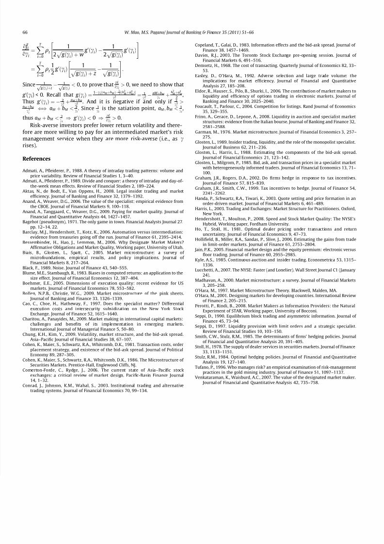
7/29/2019 Specialist, Designated Market Makers, Mao_Pagano2011JBF
http://slidepdf.com/reader/full/specialist-designated-market-makers-maopagano2011jbf 16/16
o f ioci
¼XT
t ¼0
qt
1
2 ffiffiffiffiffiffiffiffiffiffiffiffiffiffiffiffiffiffiffiffi g cið Þ þ w
p g 0 cið Þ À1
2 ffiffiffiffiffiffiffiffiffiffiffi g cið Þ
p g 0 cið Þ
" #
¼XT
t ¼0
qt
1
2 g 0 cið Þ
1 ffiffiffiffiffiffiffiffiffiffiffiffiffiffiffiffiffiffiffi g cið Þ þ z
p À1 ffiffiffiffiffiffiffiffiffiffiffi
g cið Þp
" #:
Since 1 ffiffiffiffiffiffiffiffiffiffiffi g ðciÞþ z
p À 1 ffiffiffiffiffiffiffi g ðciÞ
p < 0, to prove that o f ioci> 0, we need to show that
g 0(ci) < 0. Recall that g ðciÞ ¼1Àci
½ðaM
þbM
ÞÀci
2 ðb2
M
þa2
M Þc2i ¼ 1c2
i ÀaM
þb
M ci þb2
M
þa2
M 2 ,Thus g 0ðciÞ ¼ À 2
c3i
þ aM þbM
c2i
. And it is negative if and only if 2c3
i
>aM þbM
c2i
() aM þ bM < 2ci
. Since 1ci
is the satiation point, aM ; bM < 1ci
,
thus aM þ bM < 2ci
) g 0ðciÞ < 0 ) o f i
oci> 0.
Risk-averse investors prefer lower return volatility and there-
fore are more willing to pay for an intermediated market’s risk
management service when they are more risk-averse (i.e., as crises).
References
Admati, A., Pfleiderer, P., 1988. A theory of intraday trading patterns: volume andprice variability. Review of Financial Studies 1, 3–40.
Admati, A., Pfleiderer, P., 1989. Divide and conquer: a theory of intraday and day-of-the-week mean effects. Review of Financial Studies 2, 189–224.
Aktas, N., de Bodt, E., Van Oppens, H., 2008. Legal insider trading and marketefficiency. Journal of Banking and Finance 32, 1379–1392.
Anand, A., Weaver, D.G., 2006. The value of the specialist: empirical evidence fromthe CBOE. Journal of Financial Markets 9, 100–118.
Anand, A., Tanggaard, C., Weaver, D.G., 2009. Paying for market quality. Journal of Financial and Quantitative Analysis 44, 1427–1457.
Bagehot (pseudonym), 1971. The only game in town. Financial Analysts Journal 27.pp. 12–14, 22.
Barclay, M.J., Hendershott, T., Kotz, K., 2006. Automation versus intermediation:evidence from treasuries going off the run. Journal of Finance 61, 2395–2414.
Bessembinder, H., Hao, J., Lemmon, M., 2006. Why Designate Market Makers?Affirmative Obligations and Market Quality, Working paper, University of Utah.
Biais, B., Glosten, L., Spatt, C., 2005. Market microstructure: a survey of microfoundations, empirical results, and policy implications. Journal of Financial Markets 8, 217–264.
Black, F., 1989. Noise. Journal of Finance 43, 540–555.Blume, M.E., Stambaugh, R., 1983. Biases in computed returns: an application to the
size effect. Journal of Financial Economics 12, 387–404.Boehmer, E.E., 2005. Dimensions of execution quality: recent evidence for US
markets. Journal of Financial Economics 78, 553–582.Bollen, N.P.B., Christie, W.G., 2009. Market microstructure of the pink sheets.
Journal of Banking and Finance 33, 1326–1339.Cao, C., Choe, H., Hatheway, F., 1997. Does the specialist matter? Differential
execution costs and intersecurity subsidization on the New York StockExchange. Journal of Finance 52, 1615–1640.
Charitou, A., Panayides, M., 2009. Market making in international capital markets:challenges and benefits of its implementation in emerging markets.International Journal of Managerial Finance 5, 50–80.
Chung, K.H., Kim, Y., 2009. Volatility, market structure, and the bid-ask spread.Asia–Pacific Journal of Financial Studies 38, 67–107.
Cohen, K., Maier, S., Schwartz, R.A., Whitcomb, D.K., 1981. Transaction costs, orderplacement strategy, and existence of the bid-ask spread. Journal of PoliticalEconomy 89, 287–305.
Cohen, K., Maier, S., Schwartz, R.A., Whitcomb, D.K., 1986. The Microstructure of Securities Markets. Prentice-Hall, Englewood Cliffs, NJ.
Comerton-Forde, C., Rydge, J., 2006. The current state of Asia–Pacific stockexchanges: a critical review of market design. Pacific-Basin Finance Journal
14, 1–32.Conrad, J., Johnson, K.M., Wahal, S., 2003. Institutional trading and alternative
trading systems. Journal of Financial Economics 70, 99–134.
Copeland, T., Galai, D., 1983. Information effects and the bid-ask spread. Journal of Finance 38, 1457–1469.
Davies, R.J., 2003. The Toronto Stock Exchange pre-opening session. Journal of Financial Markets 6, 491–516.
Demsetz, H., 1968. The cost of transacting. Quarterly Journal of Economics 82, 33–53.
Easley, D., O’Hara, M., 1992. Adverse selection and large trade volume: theimplications for market efficiency. Journal of Financial and QuantitativeAnalysis 27, 185–208.
Eldor, R., Hauser, S., Pilo, B., Shurki, I., 2006. The contribution of market makers to
liquidity and efficiency of options trading in electronic markets. Journal of Banking and Finance 30, 2025–2040.
Foucault, T., Parlour, C., 2004. Competition for listings. Rand Journal of Economics35, 329–355.
Frino, A., Gerace, D., Lepone, A., 2008. Liquidity in auction and specialist marketstructures: evidence from the Italian bourse. Journal of Banking and Finance 32,2581–2588.
Garman, M., 1976. Market microstructure. Journal of Financial Economics 3, 257–275.
Glosten, L., 1989. Insider trading, liquidity, and the role of the monopolist specialist. Journal of Business 62, 211–236.
Glosten, L., Harris, L., 1988. Estimating the components of the bid-ask spread. Journal of Financial Economics 21, 123–142.
Glosten, L., Milgrom, P., 1985. Bid, ask, and transaction prices in a specialist marketwith heterogeneously informed traders. Journal of Financial Economics 13, 71–100.
Graham, J.R., Rogers, D.A., 2002. Do firms hedge in response to tax incentives. Journal of Finance 57, 815–839.
Graham, J.R., Smith, C.W., 1999. Tax incentives to hedge. Journal of Finance 54,2241–2262.
Handa, P., Schwartz, R.A., Tiwari, K., 2003. Quote setting and price formation in anorder-driven market. Journal of Financial Markets 6, 461–489.
Harris, L., 2003. Trading and Exchanges: Market Structure for Practitioners. Oxford,New York.
Hendershott, T., Moulton, P., 2008. Speed and Stock Market Quality: The NYSE’sHybrid, Working paper, Fordham University.
Ho, T., Stoll, H., 1981. Optimal dealer pricing under transactions and returnuncertainty. Journal of Financial Economics 9, 47–73.
Hollifield, B., Miller, R.A., Sandas, P., Slive, J., 2006. Estimating the gains from tradein limit-order markets. Journal of Finance 61, 2753–2804.
Jain, P.K., 2005. Financial market design and the equity premium: electronic versusfloor trading. Journal of Finance 60, 2955–2985.
Kyle, A.S., 1985. Continuous auction and insider trading. Econometrica 53, 1315–1336.
Lucchetti, A., 2007. The NYSE: Faster (and Lonelier). Wall Street Journal C1 (January24).
Madhavan, A., 2000. Market microstructure: a survey. Journal of Financial Markets
3, 205–258.O’Hara, M., 1997. Market Microstructure Theory. Blackwell, Malden, MA.O’Hara, M., 2001. Designing markets for developing countries. International Review
of Finance 2, 205–215.Perotti, P., Rindi, B., 2008. Market Makers as Information Providers: the Natural
Experiment of STAR, Working paper, University of Bocconi.Seppi, D., 1990. Equilibrium block trading and asymmetric information. Journal of
Finance 45, 73–94.Seppi, D., 1997. Liquidity provision with limit orders and a strategic specialist.
Review of Financial Studies 10, 103–150.Smith, C.W., Stulz, R.M., 1985. The determinants of firms’ hedging policies. Journal
of Financial and Quantitative Analysis 20, 391–405.Stoll, H., 1978. The supply of dealer services in securities markets. Journal of Finance
33, 1133–1151.Stulz, R.M., 1984. Optimal hedging policies. Journal of Financial and Quantitative
Analysis 19, 127–140.Tufano, P., 1996. Who manages risk? an empirical examination of risk-management
practices in the gold mining industry. Journal of Finance 51, 1097–1137.Venkataraman, K., Waisburd, A.C., 2007. The value of the designated market maker.
Journal of Financial and Quantitative Analysis 42, 735–758.
66 W. Mao, M.S. Pagano/ Journal of Banking & Finance 35 (2011) 51–66