NTNU Fakultet for naturvitenskap og teknologi Norges teknisk-naturvitenskapelige Institutt for kjemisk prosessteknologi universitet

SPECIALIZATION PROJECT SPRING 2009

TKP 4555

PROJECT TITLE:

SIMULATION, OPTIMAL OPERATION AND SELF-OPTIMIZING CONTROL OF METHANOL PROCESS

by

THEOPHILUS ARTHUR

Supervisor for the project: Date: 10 Dec. 2009 Professor Sigurd Skogestad Phd. Student Mehdi Panahi

Acknowledgement

No great achievement in life has been without the help and support of many known and unknown individuals. In the same way, this work would not have been a success without the help and support received from many individuals.

I am most indebted to God for the supply of grace, mercy, favour, love and strength through it all.

I particularly appreciate the counsel, teaching and directions received from my wonderful and supportive supervisor, Prof. Sigurd Skogestad. Your desire to teach and explain everything to me has really taught me a lot about Process Control at the industrial point of view within this short period, I greatly appreciate your leadership Prof.

The individual and combined support received from the following people during this project write up and other academic works cannot be forgotten. The combined support of Phd student Mehdi Panahi, Phd student Deeptanshu, Trimaharika Widarena and Emmanuel Mba are really appreciated and I extend my sincere thanks to you all.

i

Abstract

This project presents simulation, optimal operation and self-optimizing control of methanol. The plant capacity was estimated to be 5000tons/day. The first task was to simulate the production of syngas by using preformer and an ATR reactor. The next simulation was done for the methanol by using a Lurgi type reactor. The reactor is filled with catalyst in tubes and the heat of reaction is removed by using boiling water. The temperature along the reactor needs to be controlled since it can deactivate the catalyst.

Here, steady state optimization is performed with seven degrees of freedom with the technical objective of maximizing the yield of methanol. The degrees of freedom are flowrate of water and oxygen, pressure of the syngas, pressure of the methanol synthesis, inlet temperature of the ATR reactor, flow ratio of purge and flow ratio of purge from the methanol loop. The optimal nominal values of these were determined after the optimization.

The disturbances considered in the process were the changes in flowrate of natural gas (±20%) and the changes in the composition of the natural gas. After evaluating the loss associated with each of the degrees of freedom, it was discovered that six of these manipulated variables were good candidate control variables and flowrate of oxygen was found out to be a degree of freedom. Out of these candidate control variables, three of them was found out to be self-optimizing variables (both pressures and temperature).

ii

Contents Contents ..................................................................................................................................... ii

List of figures ..............................................................................................................................4

INTRODUCTION .....................................................................................................................1

LITERATURE REVIEW .........................................................................................................3

2.1 Methanol ...........................................................................................................................3

2.2 Reactions and thermodynamics of synthesis gas production ...............................................5

2.3 Synthesis gas production technologies ...............................................................................5

2.4 Thermodynamics and kinetics of methanol synthesis .........................................................7

2.5 Production of methanol ......................................................................................................8

2.5.1 Lurgi low-pressure methanol synthesis process............................................................8

2.5.2 ICI low-pressure methanol process ............................................................................ 10

2.5.3 Haldor Topsøe methanol process ............................................................................... 11

2.5.4 The MGC low-pressure process ................................................................................. 12

2.6 Optimization and Self-optimizing control ........................................................................ 13

PROCESS DESCRIPTION .................................................................................................... 16

3.1 Pre-reforming .................................................................................................................. 16

3.2 Autothermic reaction ....................................................................................................... 17

3.3 Separation process ........................................................................................................... 17

3.4 Compression .................................................................................................................... 18

3.5 Methanol synthesis .......................................................................................................... 18

3.6 Purification ...................................................................................................................... 21

UNISIM REVIEW .................................................................................................................. 22

4.1 Feed Conditioning ........................................................................................................... 22

4.2 Pre-reforming .................................................................................................................. 23

4.3 Autothermic reforming (ATR) ......................................................................................... 24

4.4 Methanol production ........................................................................................................ 24

4.5 Purification ...................................................................................................................... 25

RESULTS AND DISCUSSIONS ............................................................................................ 26

5.1 Degrees of Freedom Analysis .......................................................................................... 26

5.2 Optimization results ......................................................................................................... 26

iii

5.3 Disturbances .................................................................................................................... 27

CONCLUSION ....................................................................................................................... 33

REFERENCES ........................................................................................................................ 35

APPENDIX .............................................................................................................................. 37

A: Loss Evaluation ................................................................................................................ 37

B: Sensitivity analysis............................................................................................................ 38

C: Simulation in UniSim........................................................................................................ 40

NOMENCLATURE .............................................................................................................. 49

iv

List of figures 2.1: Flowsheet of Lurgi low-pressure methanol process................................................................9

2.2 Flow scheme of the low-pressure methanol process............................................................10

2.3 Flow scheme of the reaction section of the Haldor Topsøe methanol process........................10

2.4 Mitsubishi Gas chemical low-pressure methanol synthesis process.....................................11

2.5 Loss in performance when tracking variables (y) .............................................................14

3.1 Flowsheet for methanol production..................................................................................15

4.1 Feed conditioning..........................................................................................................20

4.2 Pre-reforming..............................................................................................................21

4.3 Autothermic reforming and separation.............................................................................22

4.4 Methanol production.....................................................................................................22

4.5 Purification of crude methanol.......................................................................................23

5.1 Analysis with oxygen as manipulated variable.................................................................29

5.2 Analysis with water as manipulated variable...................................................................30

1 CHAPTER

1

INTRODUCTION

Methanol is one of the most important bulk chemicals and products of natural gas. Most often

than not it is synthesized in large scale plants from syngas. The process consists of three main

parts including production of syngas, conversion of syngas to methanol and purification of the

crude methanol to obtain the desired specifications. The reactor used for the methanol synthesis

is the Lurgi-type which resembles a shell-and-tube heat exchanger than stands vertically and

operates at a low pressure. The reactions that occur in the reactor are hydrogenation of carbon

monoxide (CO), hydrogenation of carbon dioxide (CO2) and the reverse water gas shift. More

light will thrown on these reactions in the next chapter. The reactor only converts small amount

of the syngas into methanol, the unreacted syngas is either recycled or purged. Although the

process the process might look very simple, energy demands are large, both in mechanical

energy fo the syngas compression and heating and cooling at various stages in the process.

The goal of this project is to simulate the process in UniSim to produce 5000tons/day of pure

methanol. Optimization of the process will be carried out, since it is essential to obtain an

economically feasible and competetive process. The modeling of the process includes

thermodynamics of the chemical components, models of the individual unit operations. The

flowsheet was modeled at steady state since it is a very large plant has continuous operation.

Self optimizing control is also one of the areas that will be covered in this project. This topic is

not widely acknowledged, overcoming uncertainties in operation is the main reason why we have

to select the right variables to control. Control system has been arranged in a hierarchical

structure, with each layer operating on a different time scale. Generally, scheduling (weeks), site-

wide optimization (days), local optimization (hours), supervisory control (minutes) and

regulatory control (seconds). The control variable c interconnects with these layers.

The other objective of this project was to find candidate control variables that possesses good

self-optimizing properties for the methanol process, that is for which a constant policy results in

a small (economic) loss where there is uncertainty (including disturbances, implementation

errors and model errors), [18]. This selection will be done by using trial and error with different

2

process variable combination. Direct loss evaluation will also be used. Control variables should

normally include the active constraints [18], which depend strongly on the actual operation,

including cost data.

2 CHAPTER

3

LITERATURE REVIEW

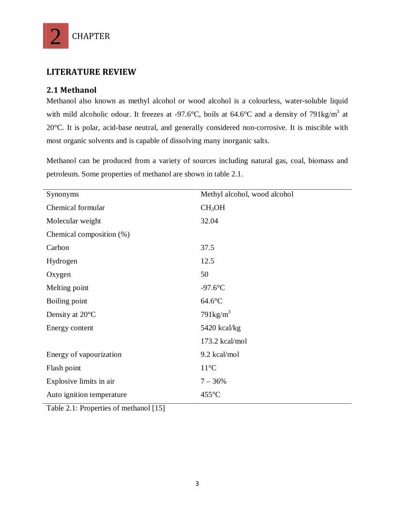
2.1 Methanol Methanol also known as methyl alcohol or wood alcohol is a colourless, water-soluble liquid

with mild alcoholic odour. It freezes at -97.6°C, boils at 64.6°C and a density of 791kg/m3 at

20°C. It is polar, acid-base neutral, and generally considered non-corrosive. It is miscible with

most organic solvents and is capable of dissolving many inorganic salts.

Methanol can be produced from a variety of sources including natural gas, coal, biomass and

petroleum. Some properties of methanol are shown in table 2.1.

Synonyms

Chemical formular

Molecular weight

Chemical composition (%)

Carbon

Hydrogen

Oxygen

Melting point

Boiling point

Density at 20°C

Energy content

Energy of vapourization

Flash point

Explosive limits in air

Auto ignition temperature

Methyl alcohol, wood alcohol

CH3OH

32.04

37.5

12.5

50

-97.6°C

64.6°C

791kg/m3

5420 kcal/kg

173.2 kcal/mol

9.2 kcal/mol

11°C

7 – 36%

455°C

Table 2.1: Properties of methanol [15]

4

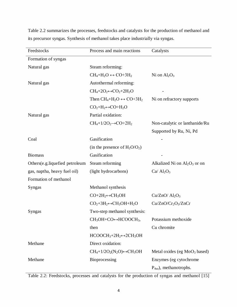
Table 2.2 summarizes the processes, feedstocks and catalysts for the production of methanol and

its precursor syngas. Synthesis of methanol takes place industrially via syngas.

Feedstocks Process and main reactions Catalysts

Formation of syngas

Natural gas

Natural gas

Natural gas

Coal

Biomass

Others(e.g.liquefied petroleum

gas, naptha, heavy fuel oil)

Formation of methanol

Syngas

Syngas

Methane

Methane

Steam reforming:

CH4+H2O ↔ CO+3H2

Autothermal reforming:

CH4+2O2↔CO2+2H2O

Then CH4+H2O ↔ CO+3H2

CO2+H2↔CO+H2O

Partial oxidation:

CH4+1/2O2→CO+2H2

Gasification

(in the presence of H2O/O2)

Gasification

Steam reforming

(light hydrocarbons)

Methanol synthesis

CO+2H2↔CH3OH

CO2+3H2↔CH3OH+H2O

Two-step methanol synthesis:

CH3OH+CO↔HCOOCH3,

then

HCOOCH3+2H2↔2CH3OH

Direct oxidation:

CH4+1/2O2(N2O)↔CH3OH

Bioprocessing

Ni on Al2O3

-

Ni on refractory supports

Non-catalytic or lanthanide/Ru

Supported by Ru, Ni, Pd

-

-

Alkalized Ni on Al2O3 or on

Ca/ Al2O3

Cu/ZnO/ Al2O3

Cu/ZnO/Cr2O3/ZnCr

Potassium methoxide

Cu chromite

Metal oxides (eg MoO3 based)

Enzymes (eg cytochrome

P4so), methanotrophs.

Table 2.2: Feedstocks, processes and catalysts for the production of syngas and methanol [15]

5

Methanol can be used as a fuel or fuel additive (e.g. neat methanol fuel, methanol blended with

gasoline, MTBE, TAME and methanol to gasoline). It can also be used for the production of

chemicals like formaldehyde, acetic acid, chloromethanes, methyl methacrylate, dimethyl

terephthalate, methyl amines, and glycol methyl ethers. It is also used as a solvent for

windshield, antifreeze, inhibitor to hydrate formation in natural gas processing and as a substrate

for crop growth.

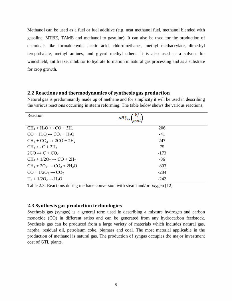
2.2 Reactions and thermodynamics of synthesis gas production Natural gas is predominantly made up of methane and for simplicity it will be used in describing the various reactions occurring in steam reforming. The table below shows the various reactions;

Reaction

CH4 + H2O ↔ CO + 3H2 206 CO + H2O ↔ CO2 + H2O -41 CH4 + CO2 ↔ 2CO + 2H2 247 CH4 ↔ C + 2H2 75 2CO ↔ C + CO2 -173 CH4 + 1/2O2 → CO + 2H2 -36 CH4 + 2O2 → CO2 + 2H2O -803 CO + 1/2O2 → CO2 -284 H2 + 1/2O2 → H2O -242 Table 2.3: Reactions during methane conversion with steam and/or oxygen [12]

2.3 Synthesis gas production technologies Synthesis gas (syngas) is a general term used in describing a mixture hydrogen and carbon monoxide (CO) in different ratios and can be generated from any hydrocarbon feedstock. Synthesis gas can be produced from a large variety of materials which includes natural gas, naptha, residual oil, petroleum coke, biomass and coal. The most material applicable in the production of methanol is natural gas. The production of syngas occupies the major investment cost of GTL plants.

6

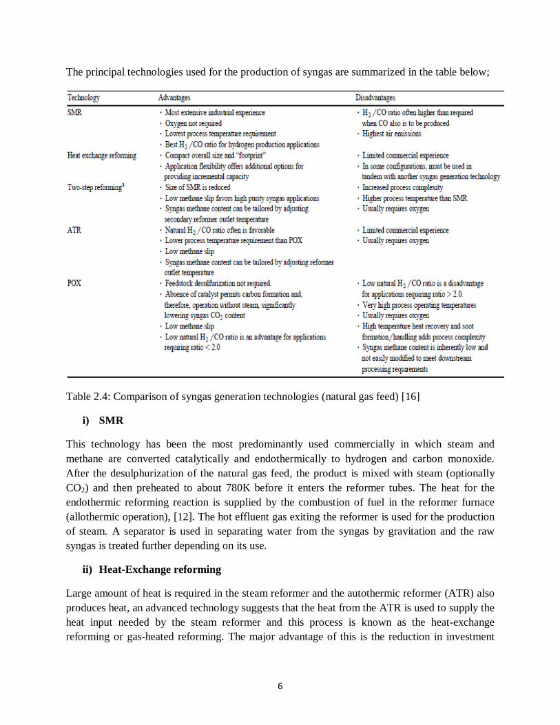
The principal technologies used for the production of syngas are summarized in the table below;

Table 2.4: Comparison of syngas generation technologies (natural gas feed) [16]

i) SMR

This technology has been the most predominantly used commercially in which steam and methane are converted catalytically and endothermically to hydrogen and carbon monoxide. After the desulphurization of the natural gas feed, the product is mixed with steam (optionally CO2) and then preheated to about 780K before it enters the reformer tubes. The heat for the endothermic reforming reaction is supplied by the combustion of fuel in the reformer furnace (allothermic operation), [12]. The hot effluent gas exiting the reformer is used for the production of steam. A separator is used in separating water from the syngas by gravitation and the raw syngas is treated further depending on its use.

ii) Heat-Exchange reforming

Large amount of heat is required in the steam reformer and the autothermic reformer (ATR) also produces heat, an advanced technology suggests that the heat from the ATR is used to supply the heat input needed by the steam reformer and this process is known as the heat-exchange reforming or gas-heated reforming. The major advantage of this is the reduction in investment

7

cost by eliminating the expensive fired reformer. The consequence of this process is that only medium pressure steam can be generated and large electrical power will be needed for the driving of the syngas compressor.

iii) Autothermic reforming (ATR)

Addition of oxygen to the steam reforming process is an alternative measure in obtaining lower H2/CO ratio. Autothermic reforming is the reforming of light hydrocarbons in a mixture of steam and oxygen in the presence of a catalyst [12]. The reactor is designed with a refractory lined vessel, therefore higher temperature and pressure can be applied than in steam reforming. ATR cannot be used alone; therefore a pre-reformer is installed downstream to it. The ATR converts the remaining methane from the pre-reformer. Air is used to supply the required oxygen.

2.4 Thermodynamics and kinetics of methanol synthesis The three main reactions for the formation of methanol from synthesis gas is made up of

hydrogenation of CO, hydrogenation of CO2 and the reverse water-gas shift reaction. The

reaction proceeds as follows;

CO + 2H2 ↔ CH3OH ∆H°298 = -90.8 kJ/mol (2.1)

CO2 + 3H2 ↔ CH3OH + H2O ∆H°298 = -49.6 kJ/mol (2.2)

CO2 + H2 ↔ CO + H2O ∆H°298 = -41 kJ/mol (2.3)

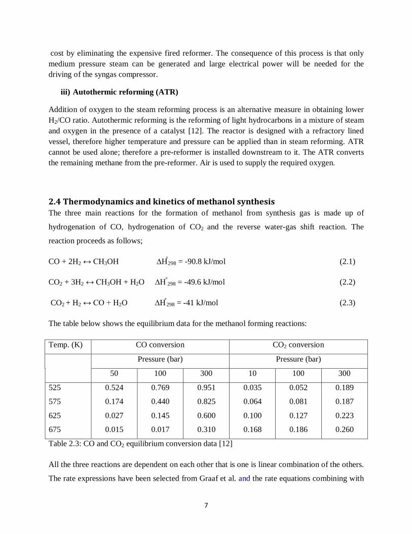
The table below shows the equilibrium data for the methanol forming reactions:

Temp. (K) CO conversion CO2 conversion

Pressure (bar) Pressure (bar)

50 100 300 10 100 300

525

575

625

675

0.524

0.174

0.027

0.015

0.769

0.440

0.145

0.017

0.951

0.825

0.600

0.310

0.035

0.064

0.100

0.168

0.052

0.081

0.127

0.186

0.189

0.187

0.223

0.260

Table 2.3: CO and CO2 equilibrium conversion data [12]

All the three reactions are dependent on each other that is one is linear combination of the others.

The rate expressions have been selected from Graaf et al. and the rate equations combining with

8

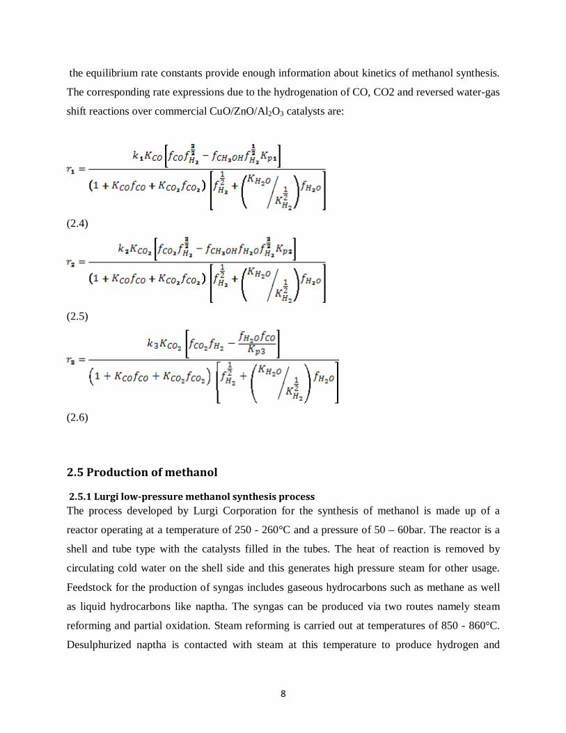
the equilibrium rate constants provide enough information about kinetics of methanol synthesis.

The corresponding rate expressions due to the hydrogenation of CO, CO2 and reversed water-gas

shift reactions over commercial CuO/ZnO/Al2O3 catalysts are:

(2.4)

(2.5)

(2.6)

2.5 Production of methanol

2.5.1 Lurgi low-pressure methanol synthesis process The process developed by Lurgi Corporation for the synthesis of methanol is made up of a

reactor operating at a temperature of 250 - 260°C and a pressure of 50 – 60bar. The reactor is a

shell and tube type with the catalysts filled in the tubes. The heat of reaction is removed by

circulating cold water on the shell side and this generates high pressure steam for other usage.

Feedstock for the production of syngas includes gaseous hydrocarbons such as methane as well

as liquid hydrocarbons like naptha. The syngas can be produced via two routes namely steam

reforming and partial oxidation. Steam reforming is carried out at temperatures of 850 - 860°C.

Desulphurized naptha is contacted with steam at this temperature to produce hydrogen and

9

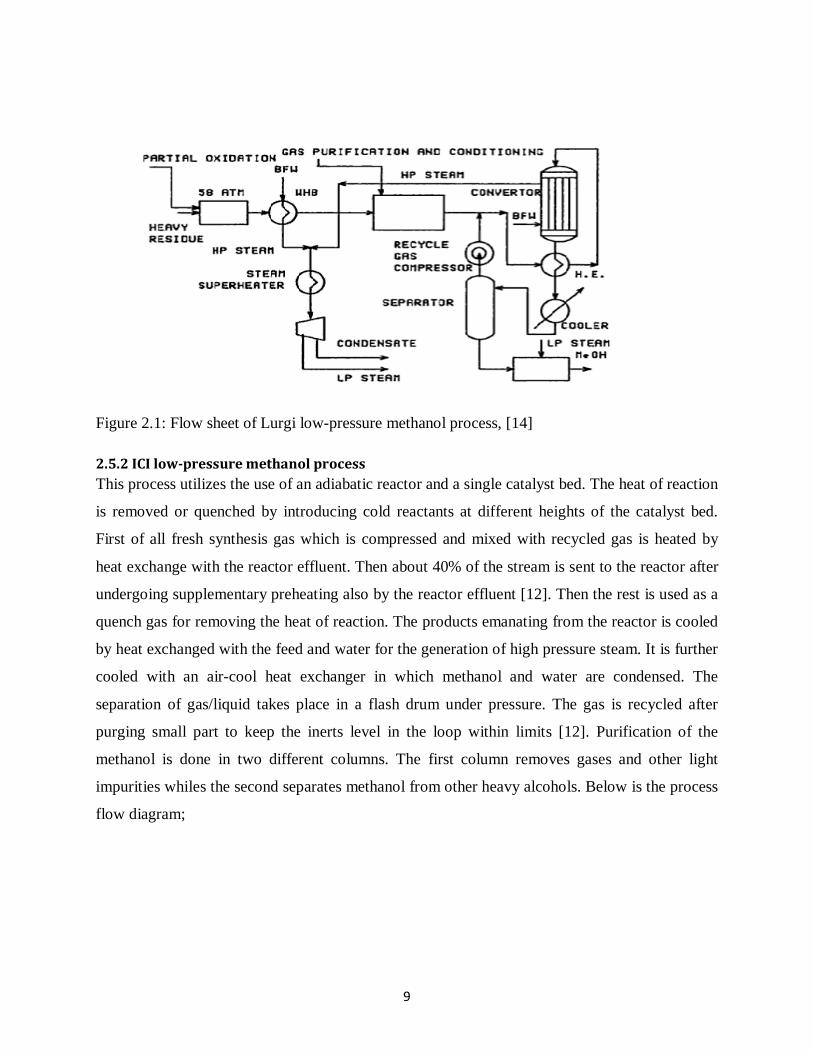
carbon oxides. The syngas produced is compressed to 50 – 80bar before it is fed into the

methanol reactor. For the second route, heavy residues are fed into a furnace along with oxygen

and steam at 1400 - 1450°C and the operating pressure is at 55 – 60bar and this does not require

any further compression. Below is the flow scheme for the process;

9

Figure 2.1: Flow sheet of Lurgi low-pressure methanol process, [14]

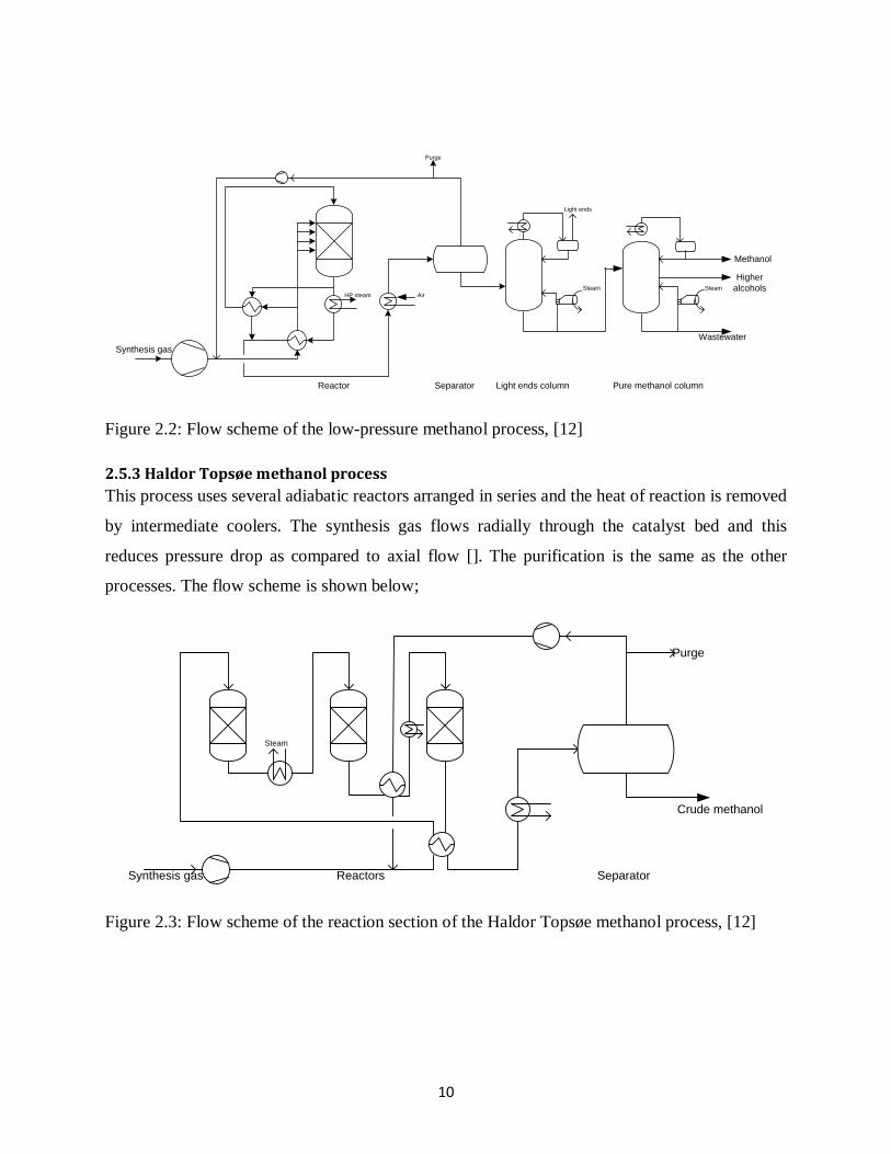
2.5.2 ICI low-pressure methanol process This process utilizes the use of an adiabatic reactor and a single catalyst bed. The heat of reaction

is removed or quenched by introducing cold reactants at different heights of the catalyst bed.

First of all fresh synthesis gas which is compressed and mixed with recycled gas is heated by

heat exchange with the reactor effluent. Then about 40% of the stream is sent to the reactor after

undergoing supplementary preheating also by the reactor effluent [12]. Then the rest is used as a

quench gas for removing the heat of reaction. The products emanating from the reactor is cooled

by heat exchanged with the feed and water for the generation of high pressure steam. It is further

cooled with an air-cool heat exchanger in which methanol and water are condensed. The

separation of gas/liquid takes place in a flash drum under pressure. The gas is recycled after

purging small part to keep the inerts level in the loop within limits [12]. Purification of the

methanol is done in two different columns. The first column removes gases and other light

impurities whiles the second separates methanol from other heavy alcohols. Below is the process

flow diagram;

10

Synthesis gas

HP steam

Reactor

Air

Separator Light ends column Pure methanol column

Steam

Wastewater

Higher alcohols

Methanol

Steam

Light ends

Purge

Figure 2.2: Flow scheme of the low-pressure methanol process, [12]

2.5.3 Haldor Topsøe methanol process This process uses several adiabatic reactors arranged in series and the heat of reaction is removed

by intermediate coolers. The synthesis gas flows radially through the catalyst bed and this

reduces pressure drop as compared to axial flow []. The purification is the same as the other

processes. The flow scheme is shown below;

Synthesis gas Reactors

Steam

Separator

Crude methanol

Purge

Figure 2.3: Flow scheme of the reaction section of the Haldor Topsøe methanol process, [12]

11

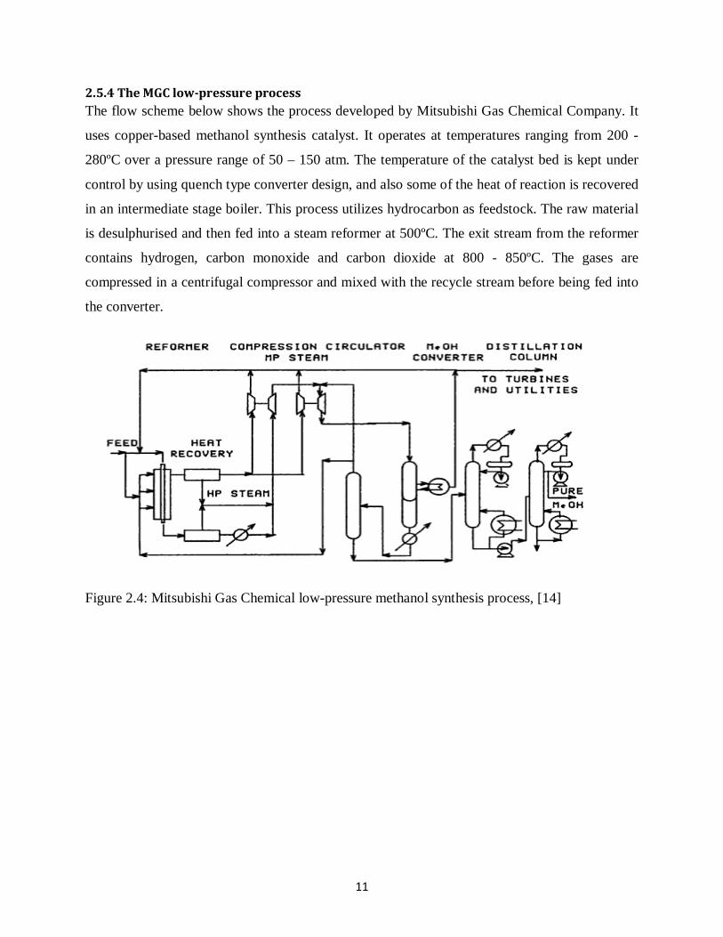
2.5.4 The MGC low-pressure process The flow scheme below shows the process developed by Mitsubishi Gas Chemical Company. It

uses copper-based methanol synthesis catalyst. It operates at temperatures ranging from 200 -

280ºC over a pressure range of 50 – 150 atm. The temperature of the catalyst bed is kept under

control by using quench type converter design, and also some of the heat of reaction is recovered

in an intermediate stage boiler. This process utilizes hydrocarbon as feedstock. The raw material

is desulphurised and then fed into a steam reformer at 500ºC. The exit stream from the reformer

contains hydrogen, carbon monoxide and carbon dioxide at 800 - 850ºC. The gases are

compressed in a centrifugal compressor and mixed with the recycle stream before being fed into

the converter.

Figure 2.4: Mitsubishi Gas Chemical low-pressure methanol synthesis process, [14]

12

2.6 Optimization and Self-optimizing control The overall control objective is to maintain acceptable operation (in terms of environmental

impact, load on operators, and so on) while keeping the operating conditions close to

economically optimal [18]. Increasing the economics of a process is the sole goal of optimization

in process industries. The economic objective is transformed into technical objectives such as

increasing the production rate and quality of the product in consideration, also decreasing the

consumption of energy as well as maintaining safe operation.

More often than not the there are constraints related to the quality and safe operation of the

product and plant respectively. The optimization problem is a mathematical representation of the

technical objectives for measuring the performance of the process. The objective function is

denoted by J in this project and it is defined as;

min Ju(u,d)

subjected to the inequality constraints

g(u,d) ≤ 0

where u are the independent variables we can affect (degrees of freedom for optimization) and d

are independent variables we cannot affect (disturbances).

The objective function J can either be maximized or minimized depending on the given problem

subjected to constraints by using available inputs and parameters u (decision variables). There a

whole lot methods used in solving the optimization problem, such methods are beyond the scope

of this project.

Self-optimizing control

Self-optimizing control is when acceptable operation (acceptable loss in the objective function)

can be achieved by using pre-calculated setpoints,c, for the controlled variables (y) (without the

use of re-optimization when disturbances occur) [18].

13

Finding such variables begins with the determination of the optimal operation (results of the

nominal optimization) and the available degrees of freedom (inputs u). Active constraints or

optimal values of variables at constraints should be controlled (“active constraint control”[18])

for optimal operation, and easy relative implementation. Control of unconstrained variables can

also be achieved by using some of the available degrees of freedom for such actions.

[19] suggests requirements for unconstrained variable control;

1. It should be easy to measure and control accurately. Small implementation error.

2. Optimal value should be insensitive to disturbances. Small optimal variations

3. It should be sensitive to changes in the manipulated variables (u). Input-output gain

should be large.

Direct Loss Evaluation

Brute force method ( Direct loss evaluation) [18] is a simple way of finding the candidate control

variables (y) and the possible disturbances (d) when they are small in numbers.

The loss (L) can be defined as the difference in the objective function for Jopt(d) and J(u,d).

L=Jopt(d) – J(u,d)

Where Jopt = J(uopt(d),d) is the result of re-optimizing the problem with the known disturbance

present in the optimization problem and J(u,d) is the result when tracking a nominal optimal

value when disturbances occur without re-optimizing the problem.

The loss for the various candidate control variables are then evaluated for the possible

disturbance. The candidate control variable (CV) with the smallest worse case or average loss

over all the disturbances is then selected as the best candidate [18].

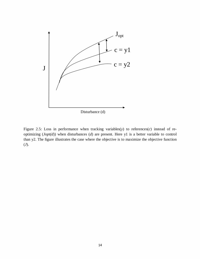
Figure 2.5 shows the objective function value for an increasing disturbance, the re-optimize case

(Jopt(d)) and two candidate control variables y1 and y2.

14

Figure 2.5: Loss in performance when tracking variables(y) to references(c) instead of re-optimizing (Jopt(d)) when disturbances (d) are present. Here y1 is a better variable to control than y2. The figure illustrates the case where the objective is to maximize the objective function (J).

J

Disturbance (d)

Jopt

c = y1

c = y2

3 CHAPTER

15

PROCESS DESCRIPTION

Heater-1

Heater-2Pre-reformer ATR reactor

Heater-3

Cooler

Compressor

Heater 4MixerSeparator

Oxygen

Natural gas

Water

Pump

Expander

Methanol reactor

Flash drum

Recycle

Purge

Vapour

Pure methanol

WaterDistillation column

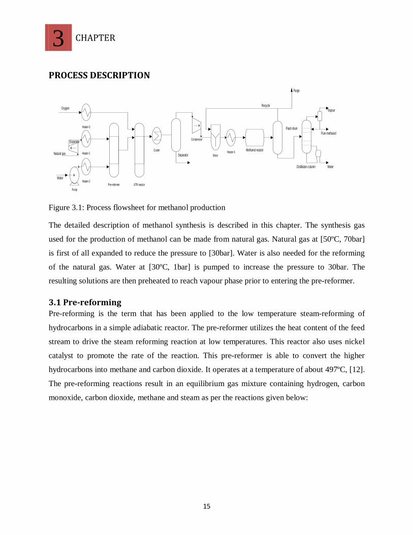
Figure 3.1: Process flowsheet for methanol production

The detailed description of methanol synthesis is described in this chapter. The synthesis gas

used for the production of methanol can be made from natural gas. Natural gas at [50ºC, 70bar]

is first of all expanded to reduce the pressure to [30bar]. Water is also needed for the reforming

of the natural gas. Water at [30ºC, 1bar] is pumped to increase the pressure to 30bar. The

resulting solutions are then preheated to reach vapour phase prior to entering the pre-reformer.

3.1 Pre-reforming Pre-reforming is the term that has been applied to the low temperature steam-reforming of

hydrocarbons in a simple adiabatic reactor. The pre-reformer utilizes the heat content of the feed

stream to drive the steam reforming reaction at low temperatures. This reactor also uses nickel

catalyst to promote the rate of the reaction. This pre-reformer is able to convert the higher

hydrocarbons into methane and carbon dioxide. It operates at a temperature of about 497ºC, [12].

The pre-reforming reactions result in an equilibrium gas mixture containing hydrogen, carbon

monoxide, carbon dioxide, methane and steam as per the reactions given below:

16

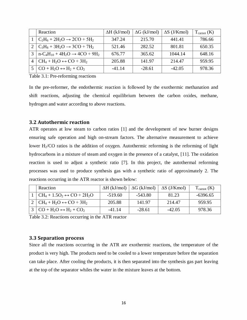
Reaction ∆H (kJ/mol) ∆G (kJ/mol) ∆S (J/Kmol) Tcarnot (K) 1 C2H6 + 2H2O → 2CO + 5H2 347.24 215.70 441.41 786.66 2 C3H8 + 3H2O → 3CO + 7H2 521.46 282.52 801.81 650.35 3 n-C4H10 + 4H2O → 4CO + 9H2 676.77 365.62 1044.14 648.16 4 CH4 + H2O ↔ CO + 3H2 205.88 141.97 214.47 959.95 5 CO + H2O ↔ H2 + CO2 -41.14 -28.61 -42.05 978.36

Table 3.1: Pre-reforming reactions In the pre-reformer, the endothermic reaction is followed by the exothermic methanation and

shift reactions, adjusting the chemical equilibrium between the carbon oxides, methane,

hydrogen and water according to above reactions.

3.2 Autothermic reaction ATR operates at low steam to carbon ratios [1] and the development of new burner designs

ensuring safe operation and high on-stream factors. The alternative measurement to achieve

lower H2/CO ratios is the addition of oxygen. Autothermic reforming is the reforming of light

hydrocarbons in a mixture of steam and oxygen in the presence of a catalyst, [11]. The oxidation

reaction is used to adjust a synthetic ratio [7]. In this project, the autothermal reforming

processes was used to produce synthesis gas with a synthetic ratio of approximately 2. The

reactions occurring in the ATR reactor is shown below:

Reaction ∆H (kJ/mol) ∆G (kJ/mol) ∆S (J/Kmol) Tcarnot (K) 1 CH4 + 1.5O2 ↔ CO + 2H2O -519.60 -543.80 81.23 -6396.65 2 CH4 + H2O ↔ CO + 3H2 205.88 141.97 214.47 959.95 3 CO + H2O ↔ H2 + CO2 -41.14 -28.61 -42.05 978.36

Table 3.2: Reactions occurring in the ATR reactor

3.3 Separation process Since all the reactions occurring in the ATR are exothermic reactions, the temperature of the

product is very high. The products need to be cooled to a lower temperature before the separation

can take place. After cooling the products, it is then separated into the synthesis gas part leaving

at the top of the separator whiles the water in the mixture leaves at the bottom.

17

3.4 Compression The pressure of the synthesis gas emanating from the separator is increase from 30bar to 80bar

and this is done by using a compressor. The compressed mixture is then mixed with a recycle

stream from the flash drum as shown in the flow sheet. The temperature of the resulting mixture

is then raised to 270ºC before it enters the methanol reactor.

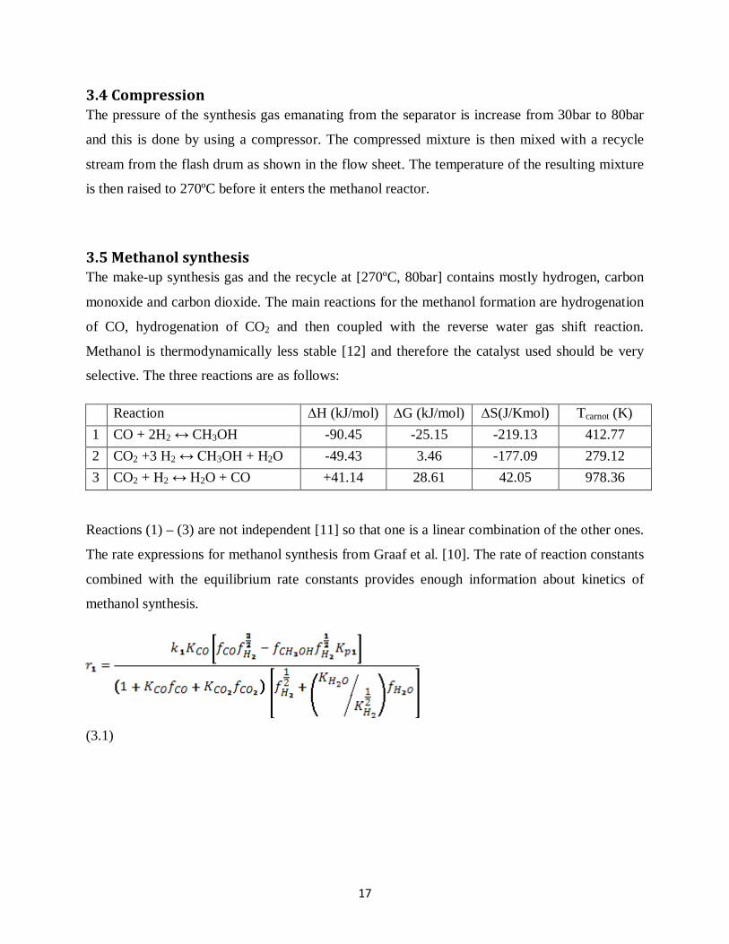
3.5 Methanol synthesis The make-up synthesis gas and the recycle at [270ºC, 80bar] contains mostly hydrogen, carbon

monoxide and carbon dioxide. The main reactions for the methanol formation are hydrogenation

of CO, hydrogenation of CO2 and then coupled with the reverse water gas shift reaction.

Methanol is thermodynamically less stable [12] and therefore the catalyst used should be very

selective. The three reactions are as follows:

Reaction ∆H (kJ/mol) ∆G (kJ/mol) ∆S(J/Kmol) Tcarnot (K) 1 CO + 2H2 ↔ CH3OH -90.45 -25.15 -219.13 412.77 2 CO2 +3 H2 ↔ CH3OH + H2O -49.43 3.46 -177.09 279.12 3 CO2 + H2 ↔ H2O + CO +41.14 28.61 42.05 978.36

Reactions (1) – (3) are not independent [11] so that one is a linear combination of the other ones.

The rate expressions for methanol synthesis from Graaf et al. [10]. The rate of reaction constants

combined with the equilibrium rate constants provides enough information about kinetics of

methanol synthesis.

(3.1)

19

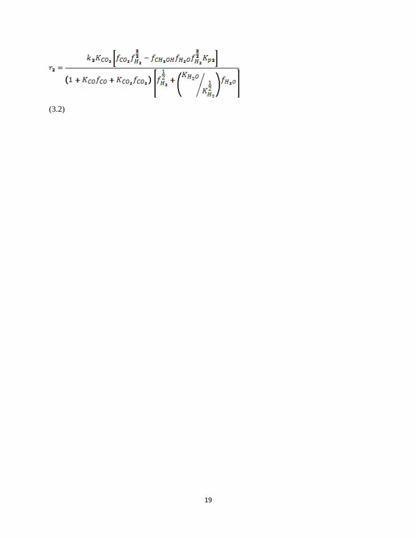
(3.2)

18

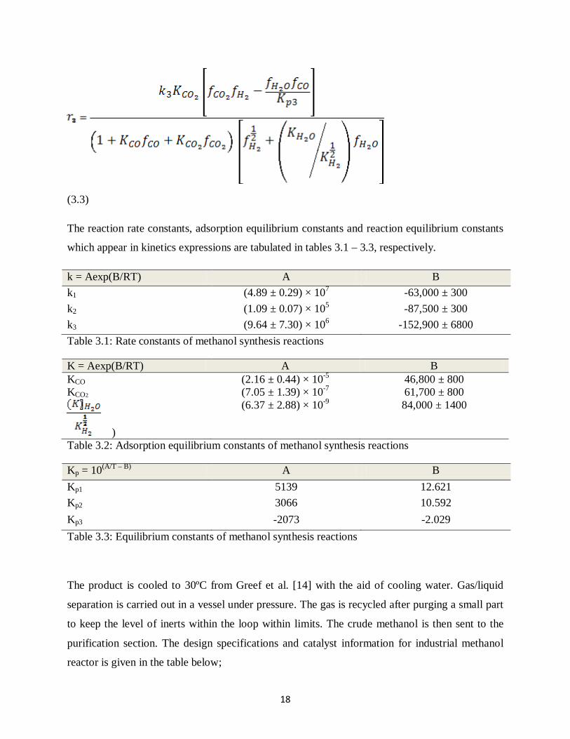
(3.3)

The reaction rate constants, adsorption equilibrium constants and reaction equilibrium constants

which appear in kinetics expressions are tabulated in tables 3.1 – 3.3, respectively.

k = Aexp(B/RT) A B k1 (4.89 ± 0.29) × 107 -63,000 ± 300 k2 (1.09 ± 0.07) × 105 -87,500 ± 300 k3 (9.64 ± 7.30) × 106 -152,900 ± 6800 Table 3.1: Rate constants of methanol synthesis reactions

K = Aexp(B/RT) A B KCO (2.16 ± 0.44) × 10-5 46,800 ± 800 KCO2 (7.05 ± 1.39) × 10-7 61,700 ± 800

)

(6.37 ± 2.88) × 10-9 84,000 ± 1400

Table 3.2: Adsorption equilibrium constants of methanol synthesis reactions

Kp = 10(A/T – B) A B Kp1 5139 12.621 Kp2 3066 10.592 Kp3 -2073 -2.029 Table 3.3: Equilibrium constants of methanol synthesis reactions

The product is cooled to 30ºC from Greef et al. [14] with the aid of cooling water. Gas/liquid

separation is carried out in a vessel under pressure. The gas is recycled after purging a small part

to keep the level of inerts within the loop within limits. The crude methanol is then sent to the

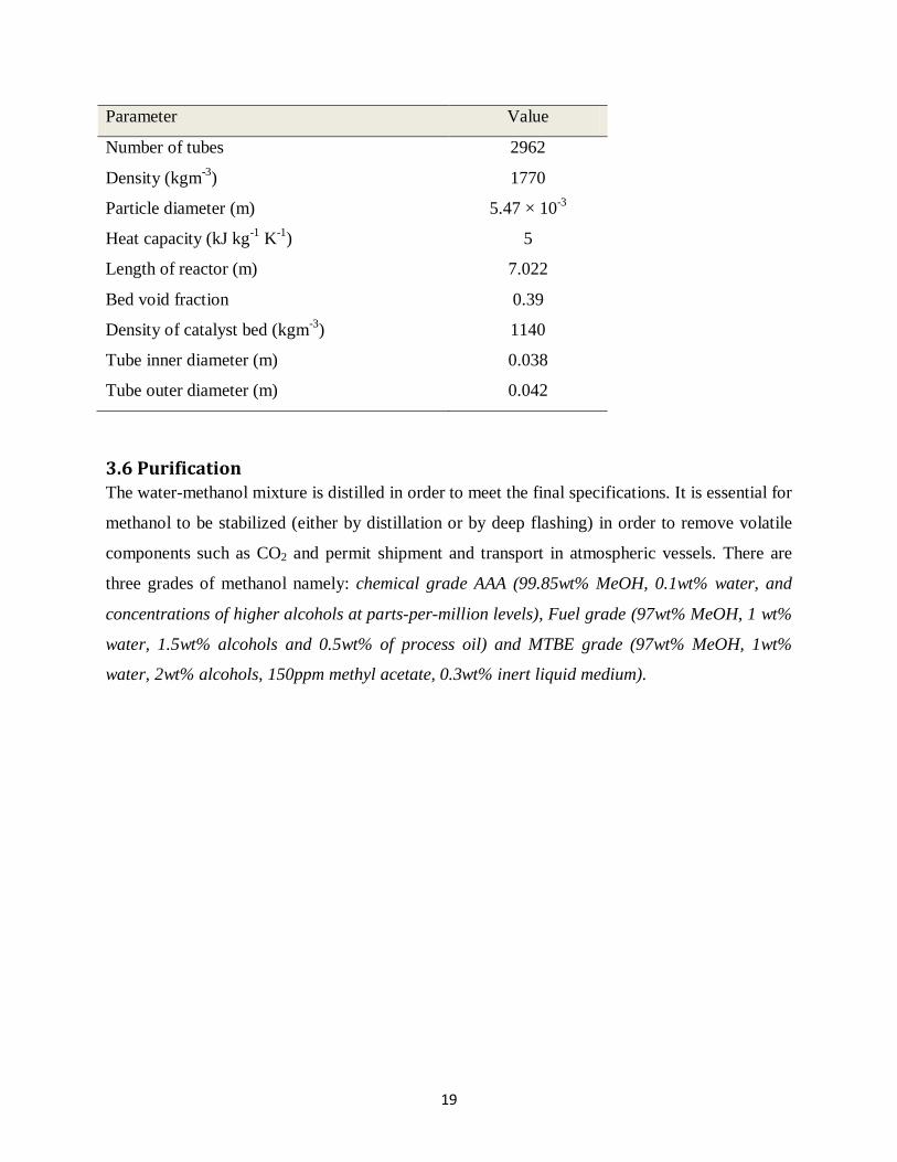
purification section. The design specifications and catalyst information for industrial methanol

reactor is given in the table below;

19

Parameter Value

Number of tubes 2962

Density (kgm-3) 1770

Particle diameter (m) 5.47 × 10-3

Heat capacity (kJ kg-1 K-1) 5

Length of reactor (m) 7.022

Bed void fraction 0.39

Density of catalyst bed (kgm-3) 1140

Tube inner diameter (m) 0.038

Tube outer diameter (m) 0.042

3.6 Purification The water-methanol mixture is distilled in order to meet the final specifications. It is essential for

methanol to be stabilized (either by distillation or by deep flashing) in order to remove volatile

components such as CO2 and permit shipment and transport in atmospheric vessels. There are

three grades of methanol namely: chemical grade AAA (99.85wt% MeOH, 0.1wt% water, and

concentrations of higher alcohols at parts-per-million levels), Fuel grade (97wt% MeOH, 1 wt%

water, 1.5wt% alcohols and 0.5wt% of process oil) and MTBE grade (97wt% MeOH, 1wt%

water, 2wt% alcohols, 150ppm methyl acetate, 0.3wt% inert liquid medium).

4 CHAPTER

20

UNISIM REVIEW Methanol production from synthesis gas is simulated using Honeywell UniSim Design R380

with Peng Robinson fluid package. The pressure drop across all the unit operations is set to 0

kPa. The simulation overview will be divided into several sections namely feed conditioning,

pre-reforming, autothermic reforming (ATR), methanol production and purification.

4.1 Feed Conditioning

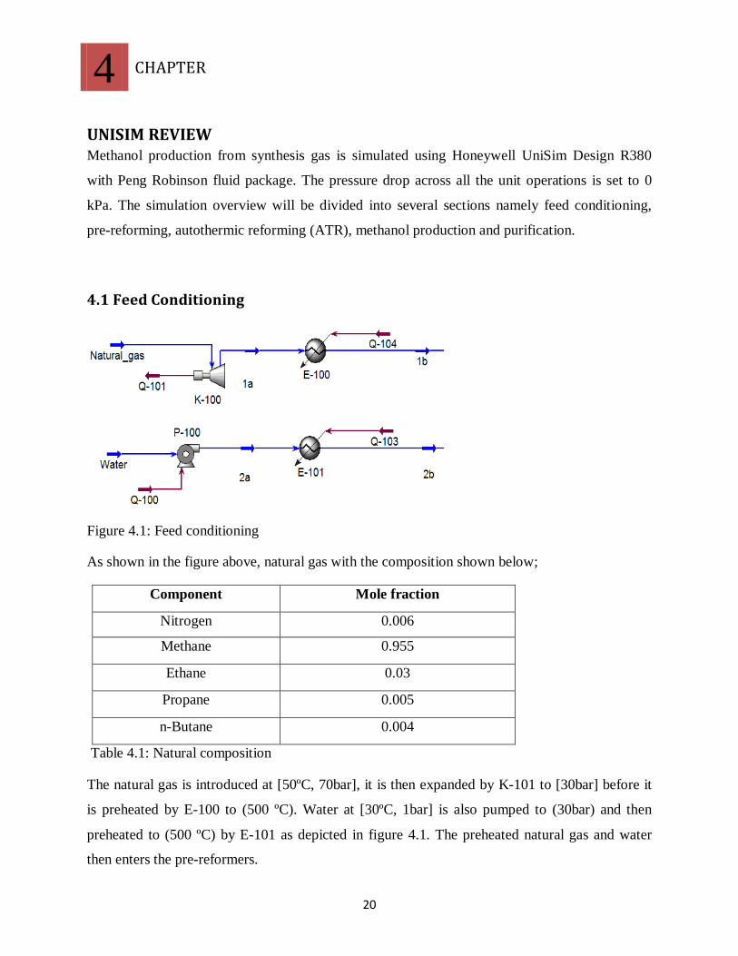
Figure 4.1: Feed conditioning

As shown in the figure above, natural gas with the composition shown below;

Component Mole fraction

Nitrogen 0.006

Methane 0.955

Ethane 0.03

Propane 0.005

n-Butane 0.004

Table 4.1: Natural composition

The natural gas is introduced at [50ºC, 70bar], it is then expanded by K-101 to [30bar] before it

is preheated by E-100 to (500 ºC). Water at [30ºC, 1bar] is also pumped to (30bar) and then

preheated to (500 ºC) by E-101 as depicted in figure 4.1. The preheated natural gas and water

then enters the pre-reformers.

23

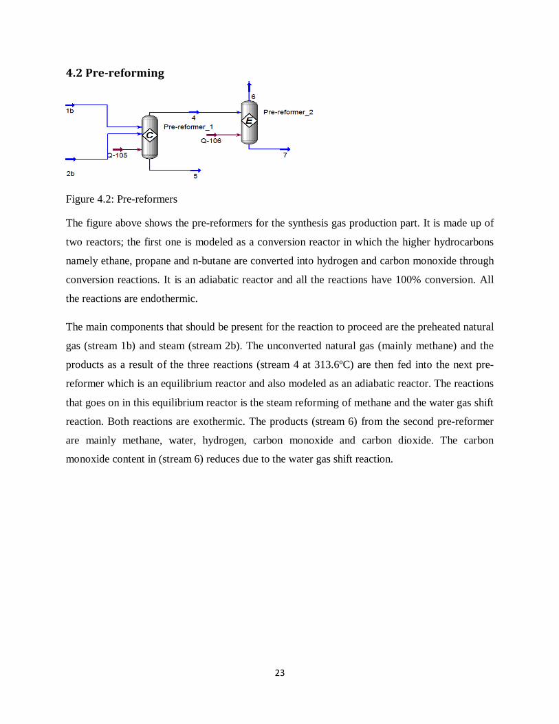
4.2 Pre-reforming

Figure 4.2: Pre-reformers

The figure above shows the pre-reformers for the synthesis gas production part. It is made up of

two reactors; the first one is modeled as a conversion reactor in which the higher hydrocarbons

namely ethane, propane and n-butane are converted into hydrogen and carbon monoxide through

conversion reactions. It is an adiabatic reactor and all the reactions have 100% conversion. All

the reactions are endothermic.

The main components that should be present for the reaction to proceed are the preheated natural

gas (stream 1b) and steam (stream 2b). The unconverted natural gas (mainly methane) and the

products as a result of the three reactions (stream 4 at 313.6ºC) are then fed into the next pre-

reformer which is an equilibrium reactor and also modeled as an adiabatic reactor. The reactions

that goes on in this equilibrium reactor is the steam reforming of methane and the water gas shift

reaction. Both reactions are exothermic. The products (stream 6) from the second pre-reformer

are mainly methane, water, hydrogen, carbon monoxide and carbon dioxide. The carbon

monoxide content in (stream 6) reduces due to the water gas shift reaction.

22

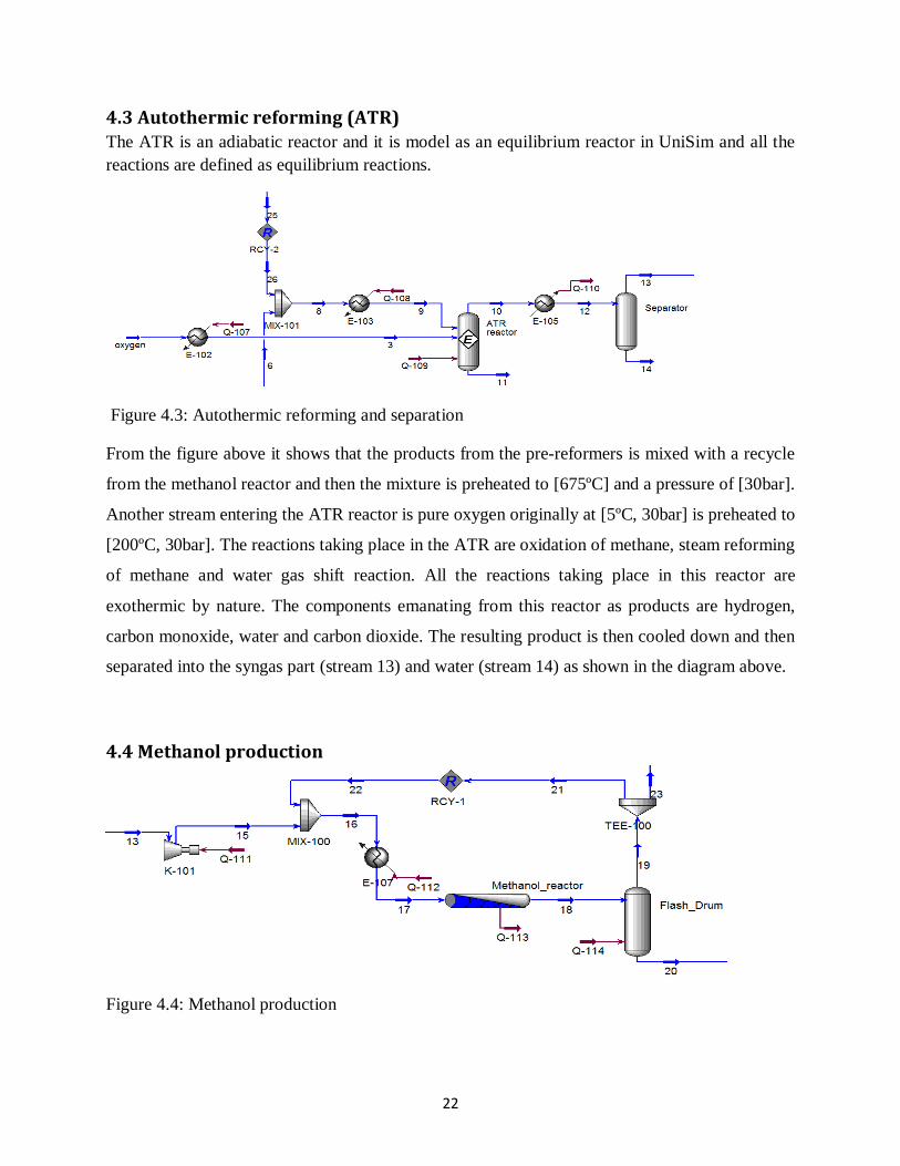
4.3 Autothermic reforming (ATR) The ATR is an adiabatic reactor and it is model as an equilibrium reactor in UniSim and all the reactions are defined as equilibrium reactions.

Figure 4.3: Autothermic reforming and separation

From the figure above it shows that the products from the pre-reformers is mixed with a recycle

from the methanol reactor and then the mixture is preheated to [675ºC] and a pressure of [30bar].

Another stream entering the ATR reactor is pure oxygen originally at [5ºC, 30bar] is preheated to

[200ºC, 30bar]. The reactions taking place in the ATR are oxidation of methane, steam reforming

of methane and water gas shift reaction. All the reactions taking place in this reactor are

exothermic by nature. The components emanating from this reactor as products are hydrogen,

carbon monoxide, water and carbon dioxide. The resulting product is then cooled down and then

separated into the syngas part (stream 13) and water (stream 14) as shown in the diagram above.

4.4 Methanol production

Figure 4.4: Methanol production

25

The synthesis gas leaving the separator is compressed to [80bar] and then mixed with the recycle

stream from the flash drum. The temperature of the mixture is then increased from [209ºC] to

[270ºC]. The methanol reactor is a plug flow reactor (PFR) with 2962 tubes inside. All the

reactions (CO hydrogenation, CO2 hydrogenation and the reverse water gas shift) are modeled as

a heterogeneous catalytic reaction and the reactions are exothermic. The exiting temperature is

specified as 250ºC. The crude methanol leaving the reactor (stream 18) at [250ºC, 80bar] is

flashed in a flash drum and the streams exiting this equipment are at a temperature of [30ºC,

80bar]. Stream [19] is recycled after purging small part to keep the level of inert in the loop

within limits. Stream [20] consisting mainly of methanol and water is then sent to the distillation

column.

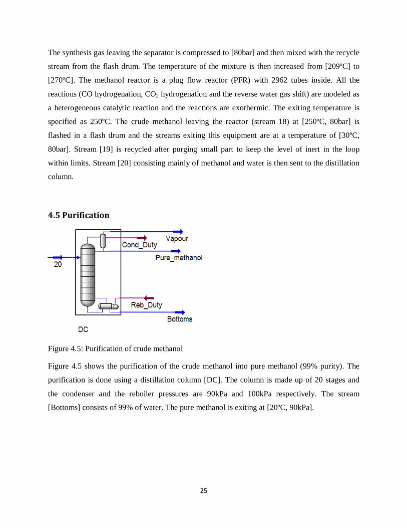
4.5 Purification

Figure 4.5: Purification of crude methanol

Figure 4.5 shows the purification of the crude methanol into pure methanol (99% purity). The

purification is done using a distillation column [DC]. The column is made up of 20 stages and

the condenser and the reboiler pressures are 90kPa and 100kPa respectively. The stream

[Bottoms] consists of 99% of water. The pure methanol is exiting at [20ºC, 90kPa].

5 CHAPTER

24

RESULTS AND DISCUSSIONS

5.1 Degrees of Freedom Analysis There are two main types of degree of freedom namely dynamic degrees of freedom Nm (m denotes manipulated) and steady state degrees of freedom Nss. Nm is usually obtained by process insight as the number of independent variables that can be manipulated by external means. Generally, it is given by the number of adjustable valves plus other adjustable mechanical and electrical devices. Nss on the other hand is the number of variables needed to be specified in order for the simulation to converge. The steady state degrees of freedom is then obtained from the equation below;

.......................................................................................................(5.1)

Where and denotes number of manipulated variables with no steady state effect and the number of variables that need to be controlled ..................respectively.

In this project since we are dealing with steady state process the manipulated variables can be specified from the process insight, which implies . The degrees of freedom (u) = output variables (y), this means we can make our selected manipulated variables to be the candidate control variables.

5.2 Optimization results In the optimization problem, the methanol production rate is set as the objective function and it is

formulated as follows:

Max J = Methanol production rate (FCH3OH).

The main objective was to find the optimal nominal values for the chosen candidate controlled

variables that was going to give us 5000ton/day of pure methanol.

Seven decision (manipulated) variables, which includes flowrate of water (FH2O) and oxygen

(FO2), synthesis gas pressure (P1), methanol synthesis pressure (P2), inlet temperature of ATR (T)

and purge from the methanol synthesis loop (R1) and ratio of purge from the plant (R2). The main

reason to develop an optimal oxygen flowrate is to give lower H2/CO ratio. Optimal inlet

temperature of ATR is chosen in order to in order to increase the amount of H2 and CO and at the

25

same time to prevent the deactivation of the catalyst and also it is because of metallurgical

constraints of the reactor vessel. Since both steam reforming and partial oxidation is hindered by

elevated pressures, the need to find an optimal pressure for the synthesis of natural gas is of

importance here. High investment cost for the compression of syngas prior to the methanol

synthesis reactor has led us to find the optimal pressure for operating the methanol reactor. The

ranges for the manipulated variables are:

3000 < FO2 < 6000 kgmole/hr

4000 < FH2O < 10000 kgmole/hr

25 < P1 < 40 bar

50 < P2 < 100 bar

0.04 < R1 < 0.1

0.1 < R2 < 0.9

600 < T < 675ºC

5.3 Disturbances The optimal operation was modeled without consideration of disturbances but this is not true in practice since there might an error with the control system of the plant. Disturbances (errors) will therefore occur since the representation is not the perfect model for the real plant.

The following disturbances (errors) were considered for this process:

• d1: Feed rate of natural gas reduced by 20% (5920 kgmole/hr) • d2: Feed rate of natural gas reduced by 15% (6290 kgmole/hr) • d3: Feed rate of natural gas reduced by 10% (6660 kgmole/hr) • d4: Feed rate of natural gas reduced by 5% (7030 kgmole/hr) • d5: Feed rate of natural gas increased by 5% (7770 kgmole/hr) • d6: Feed rate of natural gas increased by 10% (8140 kgmole/hr) • d7: Feed rate of natural gas increased by 15% (8510 kgmole/hr) • d8: Feed rate of natural gas increased by 20% (8880 kgmole/hr) • d9: Feed composition of natural gas reduced by 5% • d10: Feed composition of natural gas reduced by 10%

The base value for natural gas flowrate was 7400kgmole/hr.

26

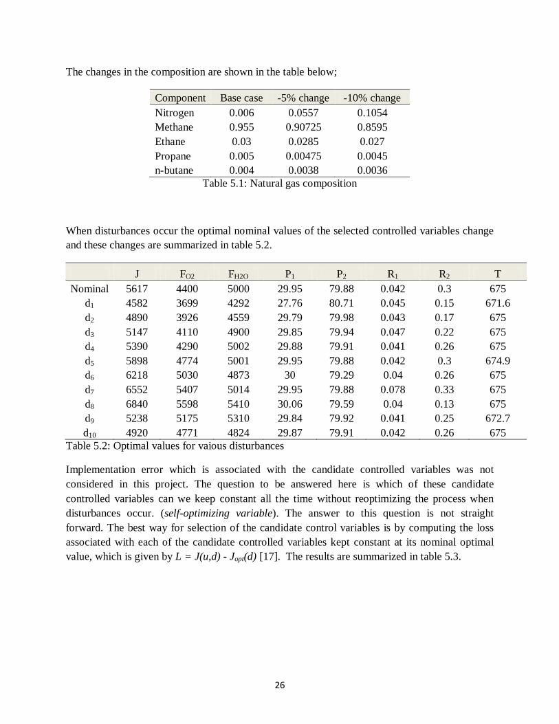
The changes in the composition are shown in the table below;

Component Base case -5% change -10% change Nitrogen 0.006 0.0557 0.1054 Methane 0.955 0.90725 0.8595 Ethane 0.03 0.0285 0.027 Propane 0.005 0.00475 0.0045 n-butane 0.004 0.0038 0.0036

Table 5.1: Natural gas composition

When disturbances occur the optimal nominal values of the selected controlled variables change and these changes are summarized in table 5.2.

J FO2 FH2O P1 P2 R1 R2 T Nominal 5617 4400 5000 29.95 79.88 0.042 0.3 675

d1 4582 3699 4292 27.76 80.71 0.045 0.15 671.6 d2 4890 3926 4559 29.79 79.98 0.043 0.17 675 d3 5147 4110 4900 29.85 79.94 0.047 0.22 675 d4 5390 4290 5002 29.88 79.91 0.041 0.26 675 d5 5898 4774 5001 29.95 79.88 0.042 0.3 674.9 d6 6218 5030 4873 30 79.29 0.04 0.26 675 d7 6552 5407 5014 29.95 79.88 0.078 0.33 675 d8 6840 5598 5410 30.06 79.59 0.04 0.13 675 d9 5238 5175 5310 29.84 79.92 0.041 0.25 672.7 d10 4920 4771 4824 29.87 79.91 0.042 0.26 675

Table 5.2: Optimal values for vaious disturbances

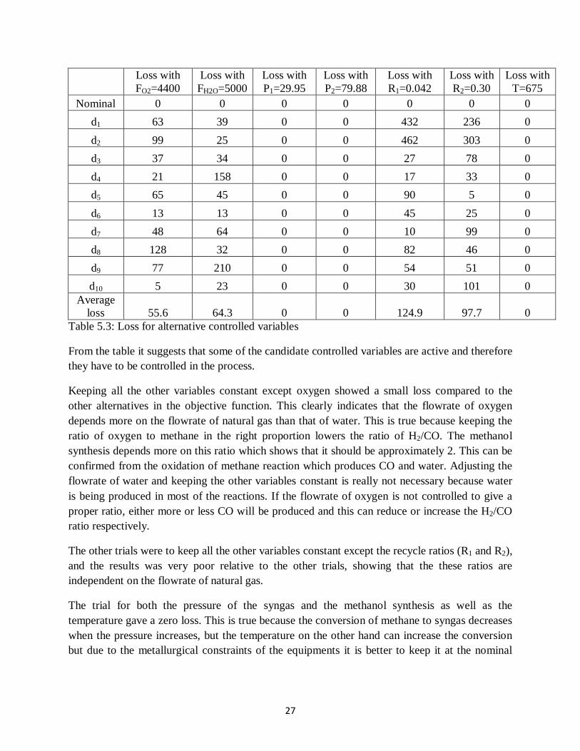
Implementation error which is associated with the candidate controlled variables was not considered in this project. The question to be answered here is which of these candidate controlled variables can we keep constant all the time without reoptimizing the process when disturbances occur. (self-optimizing variable). The answer to this question is not straight forward. The best way for selection of the candidate control variables is by computing the loss associated with each of the candidate controlled variables kept constant at its nominal optimal value, which is given by L = J(u,d) - Jopt(d) [17]. The results are summarized in table 5.3.

27

Loss with FO2=4400

Loss with FH2O=5000

Loss with P1=29.95

Loss with P2=79.88

Loss with R1=0.042

Loss with R2=0.30

Loss with T=675

Nominal 0 0 0 0 0 0 0 d1 63 39 0 0 432 236 0 d2 99 25 0 0 462 303 0 d3 37 34 0 0 27 78 0 d4 21 158 0 0 17 33 0 d5 65 45 0 0 90 5 0 d6 13 13 0 0 45 25 0 d7 48 64 0 0 10 99 0 d8 128 32 0 0 82 46 0 d9 77 210 0 0 54 51 0 d10 5 23 0 0 30 101 0

Average loss 55.6 64.3 0 0 124.9 97.7 0

Table 5.3: Loss for alternative controlled variables

From the table it suggests that some of the candidate controlled variables are active and therefore they have to be controlled in the process.

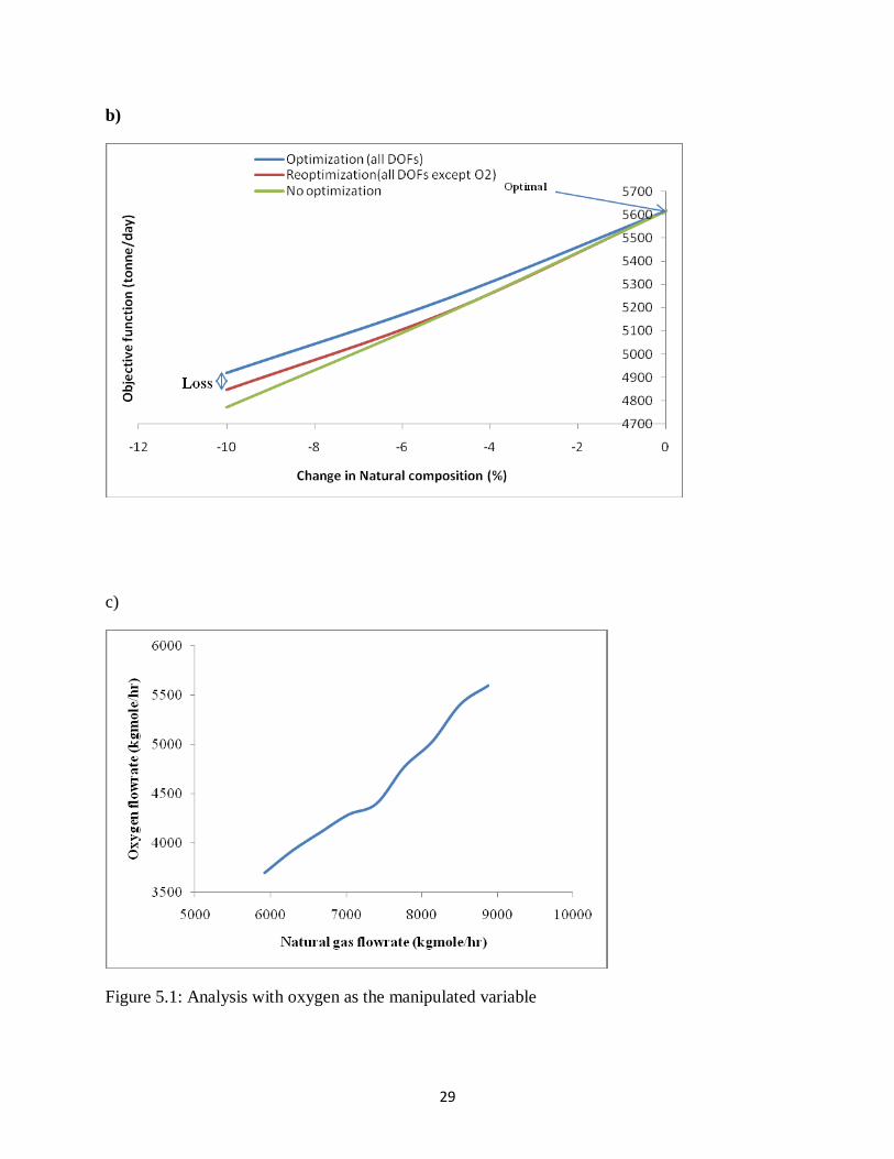
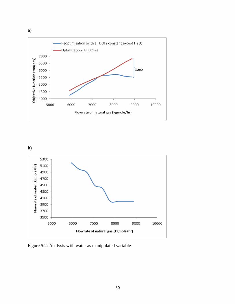
Keeping all the other variables constant except oxygen showed a small loss compared to the other alternatives in the objective function. This clearly indicates that the flowrate of oxygen depends more on the flowrate of natural gas than that of water. This is true because keeping the ratio of oxygen to methane in the right proportion lowers the ratio of H2/CO. The methanol synthesis depends more on this ratio which shows that it should be approximately 2. This can be confirmed from the oxidation of methane reaction which produces CO and water. Adjusting the flowrate of water and keeping the other variables constant is really not necessary because water is being produced in most of the reactions. If the flowrate of oxygen is not controlled to give a proper ratio, either more or less CO will be produced and this can reduce or increase the H2/CO ratio respectively.

The other trials were to keep all the other variables constant except the recycle ratios (R1 and R2), and the results was very poor relative to the other trials, showing that the these ratios are independent on the flowrate of natural gas.

The trial for both the pressure of the syngas and the methanol synthesis as well as the temperature gave a zero loss. This is true because the conversion of methane to syngas decreases when the pressure increases, but the temperature on the other hand can increase the conversion but due to the metallurgical constraints of the equipments it is better to keep it at the nominal

28

optimal value. These three variables are our active constarints in this process, controlling them is very necessary.

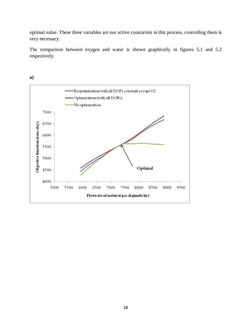
The comparison between oxygen and water is shown graphically in figures 5.1 and 5.2 respectively.

a)

29

b)

c)

Figure 5.1: Analysis with oxygen as the manipulated variable

30

a)

b)

Figure 5.2: Analysis with water as manipulated variable

6 CHAPTER

31

CONCLUSION

Simulation

In this project a methanol plant with a production rate of 5000tons/day is simulated with UniSim by using information obtained from literature. There were uncertainties in some of the parameters used for the simulation of the methanol reactor. A typical example is the number of tubes in the reactor, there were different values suggested by literature. The heterogenous kinetics used also contained some uncertainties, since no experiment was performed to find out these expressions in the project. Therefore it cannot be confidently concluded that this process mimics a real process plant.

Optimization

With refernce to the developed simulated process it became obvious that the performance of a methanol plant can be improved by changing the operating conditions from what is practised in industries. Seven variables were chosen as the degree of freedom (manipulated) variables and their optimal nominal values were obtained after the optimization.

It was assumed that y = u, this then automatically transforms the degree of freedoms to candidate control variables (CVs). Loss evaluation was performed on each of these variables by keeping six of them constant whiles one is allowed to fluctuate. After the computation it was found that the best way of running this plant is by keeping the variables FH2O, P1, P2, R1,R2 and T at their nominal optimal values while the flowrate of oxygen is manipulated. The candidate control variables are then the six mentioned above.

The self-optimizing variables found were P1, P2, and T, since keeping them constant gave the same value for the objective function as when the process was reoptimized in the presence of disturbances. The disturbances considered in the project were ±20% change in the flowrate of natural gas flowrate and also -5% and -10% change in the composition of natural gas.

Recommendation

It would have been a good idea for the one simulating the process to have at least some kind of exposure to the process by visiting an operating plant to have a look at how things are done over there.

32

Also more combinations should have been done with the candidate control variables to see if there might be a more proper self-optimizing variable will be found relative to the ones found in this project. This was not done due to time constraints.

Further work

This projects needs to be continued, so that it can be extended into the dynamic mode to see how the plant behaves in reality. A good control variable should be detected for the manipulated variable flowrate of oxygen. Heat integration sholud also be considered to cut down cost in the process. Equipment sizing, developing some control structures is also another task to be looked at in the future. The other idea is to look at incorporating a CO2 capturing plant to remove some of the CO2 from the syngas before it enters the methanol reactor.

33

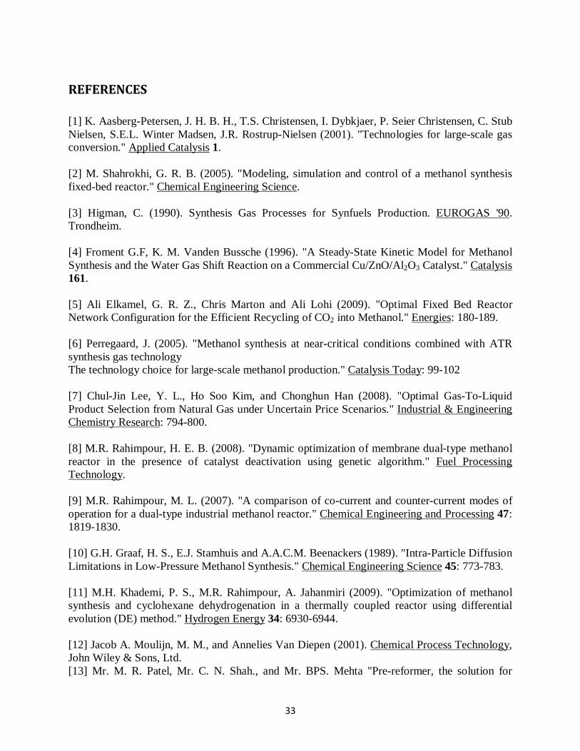
REFERENCES [1] K. Aasberg-Petersen, J. H. B. H., T.S. Christensen, I. Dybkjaer, P. Seier Christensen, C. Stub Nielsen, S.E.L. Winter Madsen, J.R. Rostrup-Nielsen (2001). "Technologies for large-scale gas conversion." Applied Catalysis 1. [2] M. Shahrokhi, G. R. B. (2005). "Modeling, simulation and control of a methanol synthesis fixed-bed reactor." Chemical Engineering Science. [3] Higman, C. (1990). Synthesis Gas Processes for Synfuels Production. EUROGAS '90. Trondheim. [4] Froment G.F, K. M. Vanden Bussche (1996). "A Steady-State Kinetic Model for Methanol Synthesis and the Water Gas Shift Reaction on a Commercial Cu/ZnO/Al2O3 Catalyst." Catalysis 161. [5] Ali Elkamel, G. R. Z., Chris Marton and Ali Lohi (2009). "Optimal Fixed Bed Reactor Network Configuration for the Efficient Recycling of CO2 into Methanol." Energies: 180-189. [6] Perregaard, J. (2005). "Methanol synthesis at near-critical conditions combined with ATR synthesis gas technology The technology choice for large-scale methanol production." Catalysis Today: 99-102 [7] Chul-Jin Lee, Y. L., Ho Soo Kim, and Chonghun Han (2008). "Optimal Gas-To-Liquid Product Selection from Natural Gas under Uncertain Price Scenarios." Industrial & Engineering Chemistry Research: 794-800. [8] M.R. Rahimpour, H. E. B. (2008). "Dynamic optimization of membrane dual-type methanol reactor in the presence of catalyst deactivation using genetic algorithm." Fuel Processing Technology. [9] M.R. Rahimpour, M. L. (2007). "A comparison of co-current and counter-current modes of operation for a dual-type industrial methanol reactor." Chemical Engineering and Processing 47: 1819-1830. [10] G.H. Graaf, H. S., E.J. Stamhuis and A.A.C.M. Beenackers (1989). "Intra-Particle Diffusion Limitations in Low-Pressure Methanol Synthesis." Chemical Engineering Science 45: 773-783. [11] M.H. Khademi, P. S., M.R. Rahimpour, A. Jahanmiri (2009). "Optimization of methanol synthesis and cyclohexane dehydrogenation in a thermally coupled reactor using differential evolution (DE) method." Hydrogen Energy 34: 6930-6944. [12] Jacob A. Moulijn, M. M., and Annelies Van Diepen (2001). Chemical Process Technology, John Wiley & Sons, Ltd. [13] Mr. M. R. Patel, Mr. C. N. Shah., and Mr. BPS. Mehta "Pre-reformer, the solution for

36

increasing plant throughput." [14] Lee, S. (1990). Methanol Synthesis Technology, CRC Press. [15] Wu-Hsun Cheng and Harold H. Kung Ed. (1994). Methanol Production and Use Chemical Industries, CRC Press. [16] D.J. Wilhelm, D. R. S., A.D. Karp, R.L. Dickenson (2001). "Syngas production for gas-to-liquids applications: technologies, issues and outlook." Fuel Processing Technology 71: 139 - 148.

[17] Sigurd Skogestad (2000). Plantwide control: the search for the self-optimizing control structure. ”Journal of Process Control” 10: 487 – 507.

[18]S. Skogestad and I. Postlethwaite (2005). Multivariable Feedback Control, 2nd edition, John Wiley & Sons Ltd.

[19] I.L Greeff, J.A. Visser, K.J. Ptasinski, F.J.J.G Janssen (2002). ”Utilization of reactor heat in methanol senthesis to reduce compressor duty-application of power cycle principles and simulation tools.” Applied thermal Engineering” 22: 1549 – 1558.

37

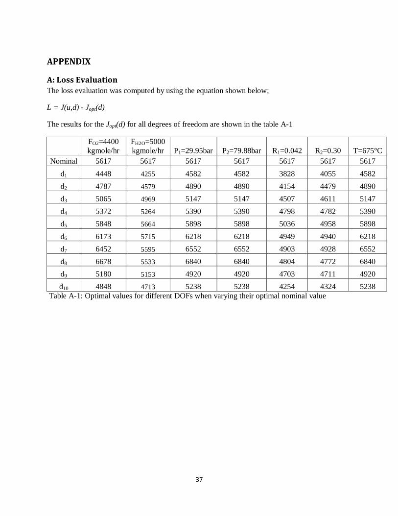
APPENDIX

A: Loss Evaluation The loss evaluation was computed by using the equation shown below;

L = J(u,d) - Jopt(d)

The results for the Jopt(d) for all degrees of freedom are shown in the table A-1

FO2=4400 kgmole/hr

FH2O=5000 kgmole/hr P1=29.95bar P2=79.88bar R1=0.042 R2=0.30 T=675°C

Nominal 5617 5617 5617 5617 5617 5617 5617 d1 4448 4255 4582 4582 3828 4055 4582 d2 4787 4579 4890 4890 4154 4479 4890 d3 5065 4969 5147 5147 4507 4611 5147 d4 5372 5264 5390 5390 4798 4782 5390 d5 5848 5664 5898 5898 5036 4958 5898 d6 6173 5715 6218 6218 4949 4940 6218 d7 6452 5595 6552 6552 4903 4928 6552 d8 6678 5533 6840 6840 4804 4772 6840 d9 5180 5153 4920 4920 4703 4711 4920 d10 4848 4713 5238 5238 4254 4324 5238

Table A-1: Optimal values for different DOFs when varying their optimal nominal value

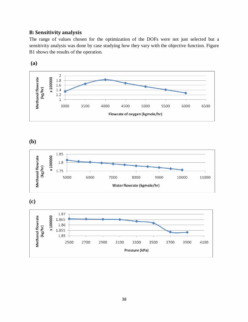
38

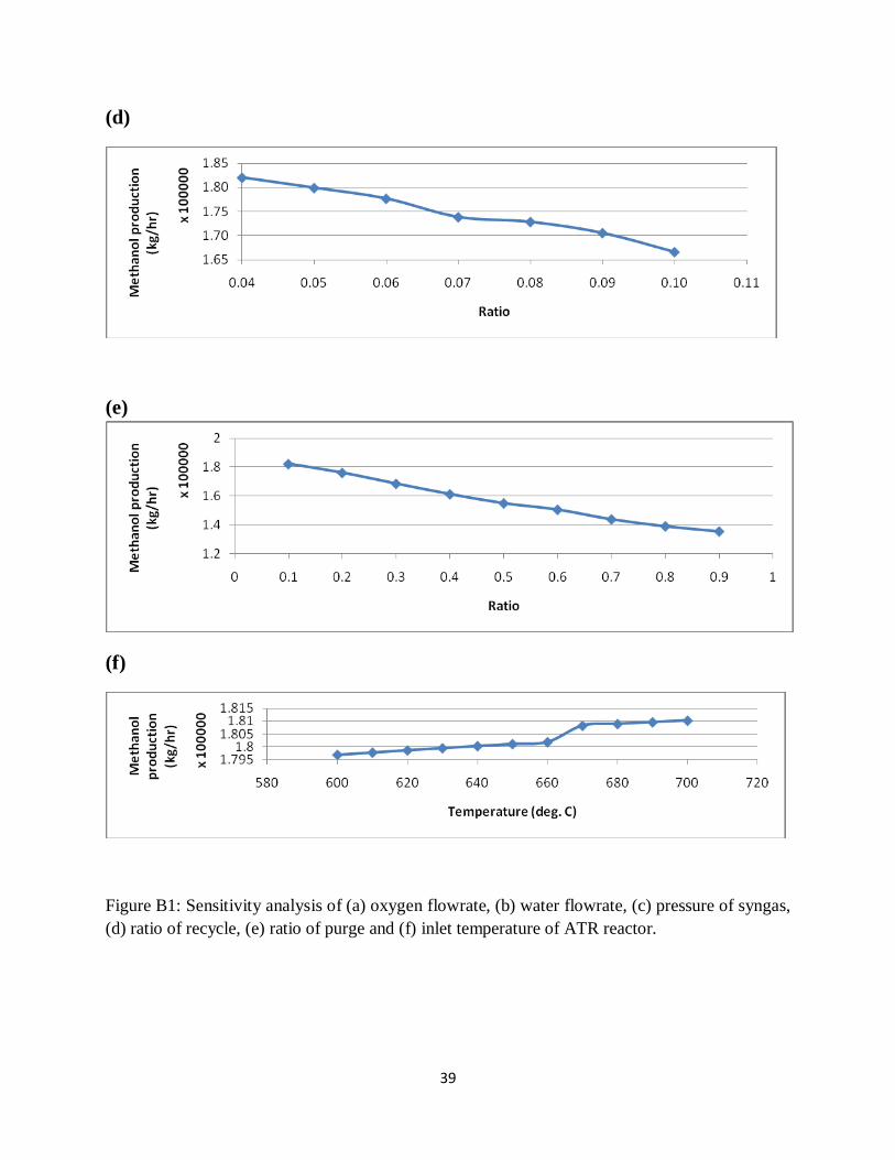
B: Sensitivity analysis The range of values chosen for the optimization of the DOFs were not just selected but a sensitivity analysis was done by case studying how they vary with the objective function. Figure B1 shows the results of the operation.

(a)

(b)

(c)

39

(d)

(e)

(f)

Figure B1: Sensitivity analysis of (a) oxygen flowrate, (b) water flowrate, (c) pressure of syngas, (d) ratio of recycle, (e) ratio of purge and (f) inlet temperature of ATR reactor.

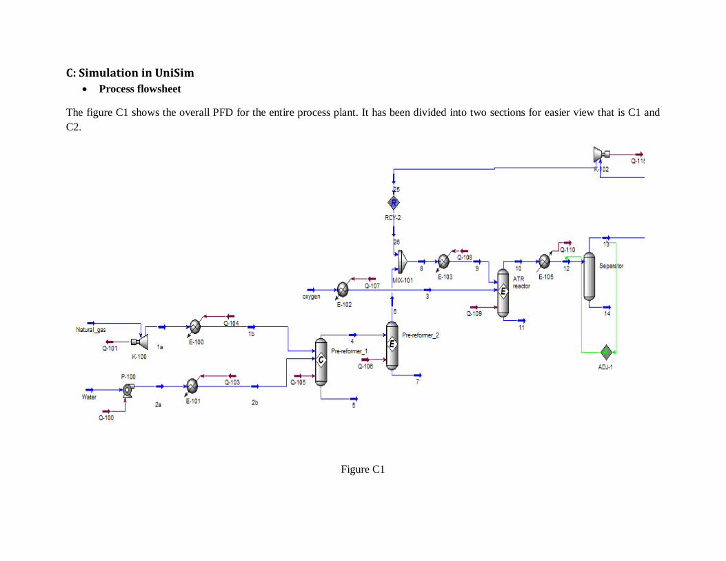
C: Simulation in UniSim • Process flowsheet

The figure C1 shows the overall PFD for the entire process plant. It has been divided into two sections for easier view that is C1 and C2.

Figure C1

41

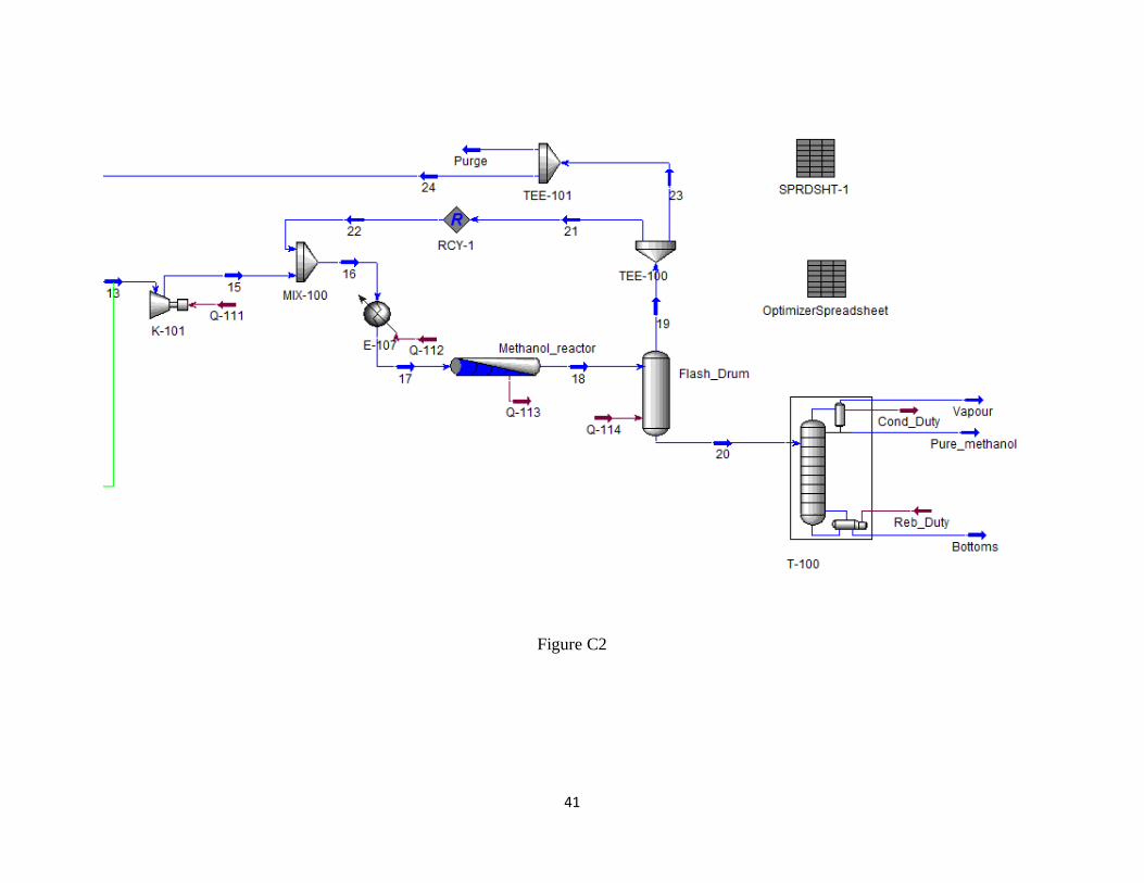
Figure C2

42

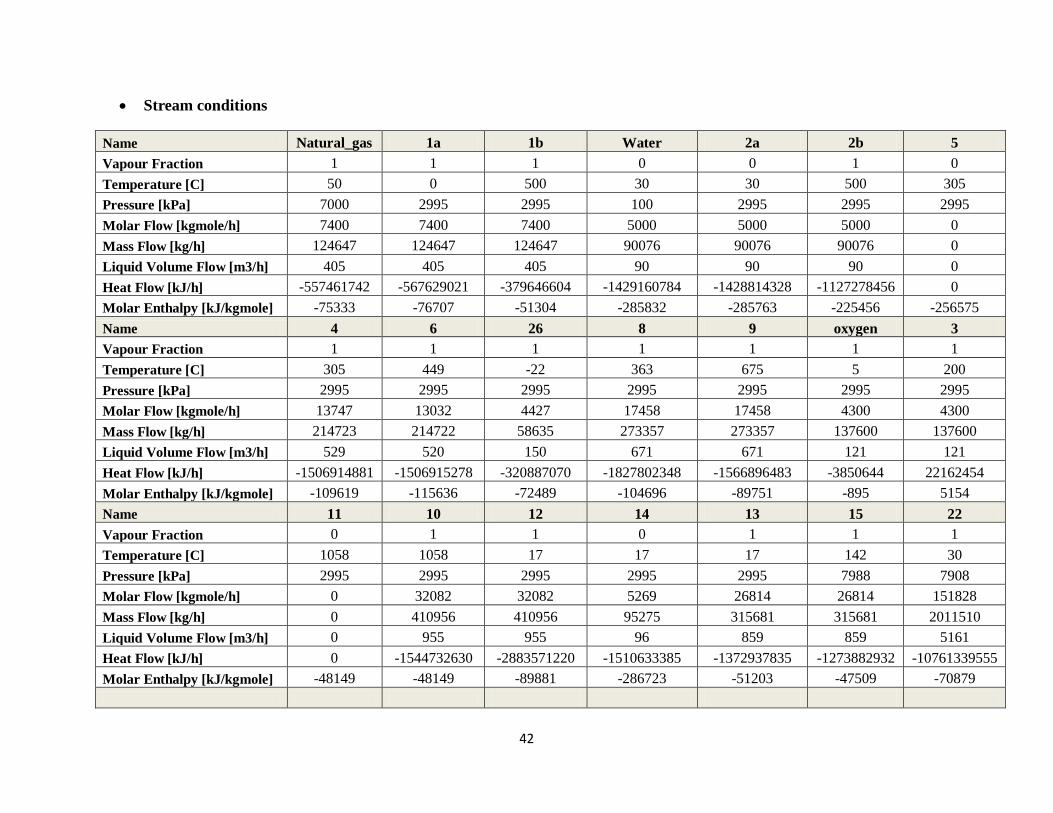
• Stream conditions

Name Natural_gas 1a 1b Water 2a 2b 5 Vapour Fraction 1 1 1 0 0 1 0 Temperature [C] 50 0 500 30 30 500 305 Pressure [kPa] 7000 2995 2995 100 2995 2995 2995 Molar Flow [kgmole/h] 7400 7400 7400 5000 5000 5000 0 Mass Flow [kg/h] 124647 124647 124647 90076 90076 90076 0 Liquid Volume Flow [m3/h] 405 405 405 90 90 90 0 Heat Flow [kJ/h] -557461742 -567629021 -379646604 -1429160784 -1428814328 -1127278456 0 Molar Enthalpy [kJ/kgmole] -75333 -76707 -51304 -285832 -285763 -225456 -256575 Name 4 6 26 8 9 oxygen 3 Vapour Fraction 1 1 1 1 1 1 1 Temperature [C] 305 449 -22 363 675 5 200 Pressure [kPa] 2995 2995 2995 2995 2995 2995 2995 Molar Flow [kgmole/h] 13747 13032 4427 17458 17458 4300 4300 Mass Flow [kg/h] 214723 214722 58635 273357 273357 137600 137600 Liquid Volume Flow [m3/h] 529 520 150 671 671 121 121 Heat Flow [kJ/h] -1506914881 -1506915278 -320887070 -1827802348 -1566896483 -3850644 22162454 Molar Enthalpy [kJ/kgmole] -109619 -115636 -72489 -104696 -89751 -895 5154 Name 11 10 12 14 13 15 22 Vapour Fraction 0 1 1 0 1 1 1 Temperature [C] 1058 1058 17 17 17 142 30 Pressure [kPa] 2995 2995 2995 2995 2995 7988 7908 Molar Flow [kgmole/h] 0 32082 32082 5269 26814 26814 151828 Mass Flow [kg/h] 0 410956 410956 95275 315681 315681 2011510 Liquid Volume Flow [m3/h] 0 955 955 96 859 859 5161 Heat Flow [kJ/h] 0 -1544732630 -2883571220 -1510633385 -1372937835 -1273882932 -10761339555 Molar Enthalpy [kJ/kgmole] -48149 -48149 -89881 -286723 -51203 -47509 -70879

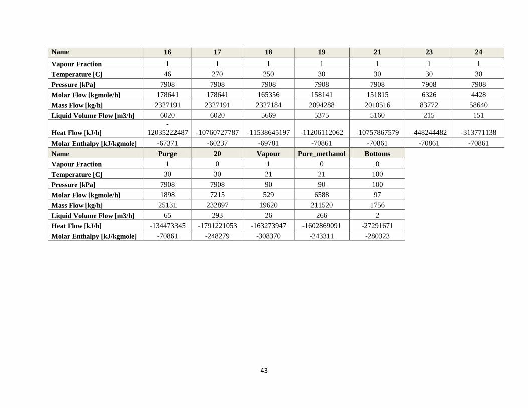
43

Name 16 17 18 19 21 23 24 Vapour Fraction 1 1 1 1 1 1 1 Temperature [C] 46 270 250 30 30 30 30 Pressure [kPa] 7908 7908 7908 7908 7908 7908 7908 Molar Flow [kgmole/h] 178641 178641 165356 158141 151815 6326 4428 Mass Flow [kg/h] 2327191 2327191 2327184 2094288 2010516 83772 58640 Liquid Volume Flow [m3/h] 6020 6020 5669 5375 5160 215 151

Heat Flow [kJ/h] -

12035222487 -10760727787 -11538645197 -11206112062 -10757867579 -448244482 -313771138 Molar Enthalpy [kJ/kgmole] -67371 -60237 -69781 -70861 -70861 -70861 -70861 Name Purge 20 Vapour Pure_methanol Bottoms Vapour Fraction 1 0 1 0 0 Temperature [C] 30 30 21 21 100 Pressure [kPa] 7908 7908 90 90 100 Molar Flow [kgmole/h] 1898 7215 529 6588 97 Mass Flow [kg/h] 25131 232897 19620 211520 1756 Liquid Volume Flow [m3/h] 65 293 26 266 2 Heat Flow [kJ/h] -134473345 -1791221053 -163273947 -1602869091 -27291671 Molar Enthalpy [kJ/kgmole] -70861 -248279 -308370 -243311 -280323

44

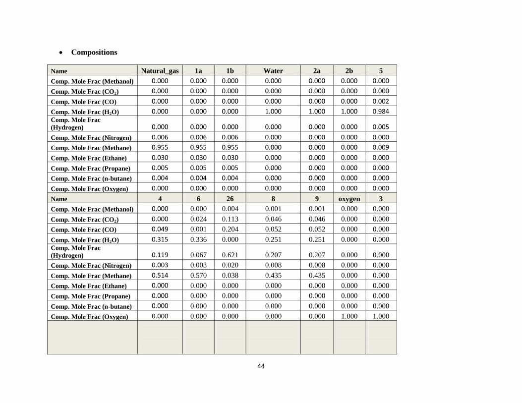
• Compositions

Name Natural_gas 1a 1b Water 2a 2b 5 Comp. Mole Frac (Methanol) 0.000 0.000 0.000 0.000 0.000 0.000 0.000 Comp. Mole Frac (CO2) 0.000 0.000 0.000 0.000 0.000 0.000 0.000 Comp. Mole Frac (CO) 0.000 0.000 0.000 0.000 0.000 0.000 0.002 Comp. Mole Frac (H2O) 0.000 0.000 0.000 1.000 1.000 1.000 0.984 Comp. Mole Frac (Hydrogen) 0.000 0.000 0.000 0.000 0.000 0.000 0.005 Comp. Mole Frac (Nitrogen) 0.006 0.006 0.006 0.000 0.000 0.000 0.000 Comp. Mole Frac (Methane) 0.955 0.955 0.955 0.000 0.000 0.000 0.009 Comp. Mole Frac (Ethane) 0.030 0.030 0.030 0.000 0.000 0.000 0.000 Comp. Mole Frac (Propane) 0.005 0.005 0.005 0.000 0.000 0.000 0.000 Comp. Mole Frac (n-butane) 0.004 0.004 0.004 0.000 0.000 0.000 0.000 Comp. Mole Frac (Oxygen) 0.000 0.000 0.000 0.000 0.000 0.000 0.000 Name 4 6 26 8 9 oxygen 3 Comp. Mole Frac (Methanol) 0.000 0.000 0.004 0.001 0.001 0.000 0.000 Comp. Mole Frac (CO2) 0.000 0.024 0.113 0.046 0.046 0.000 0.000 Comp. Mole Frac (CO) 0.049 0.001 0.204 0.052 0.052 0.000 0.000 Comp. Mole Frac (H2O) 0.315 0.336 0.000 0.251 0.251 0.000 0.000 Comp. Mole Frac (Hydrogen) 0.119 0.067 0.621 0.207 0.207 0.000 0.000 Comp. Mole Frac (Nitrogen) 0.003 0.003 0.020 0.008 0.008 0.000 0.000 Comp. Mole Frac (Methane) 0.514 0.570 0.038 0.435 0.435 0.000 0.000 Comp. Mole Frac (Ethane) 0.000 0.000 0.000 0.000 0.000 0.000 0.000 Comp. Mole Frac (Propane) 0.000 0.000 0.000 0.000 0.000 0.000 0.000 Comp. Mole Frac (n-butane) 0.000 0.000 0.000 0.000 0.000 0.000 0.000 Comp. Mole Frac (Oxygen) 0.000 0.000 0.000 0.000 0.000 1.000 1.000

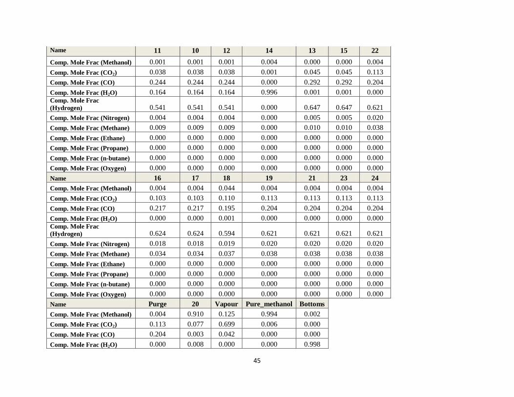
45

Name 11 10 12 14 13 15 22 Comp. Mole Frac (Methanol) 0.001 0.001 0.001 0.004 0.000 0.000 0.004 Comp. Mole Frac (CO2) 0.038 0.038 0.038 0.001 0.045 0.045 0.113 Comp. Mole Frac (CO) 0.244 0.244 0.244 0.000 0.292 0.292 0.204 Comp. Mole Frac (H2O) 0.164 0.164 0.164 0.996 0.001 0.001 0.000 Comp. Mole Frac (Hydrogen) 0.541 0.541 0.541 0.000 0.647 0.647 0.621 Comp. Mole Frac (Nitrogen) 0.004 0.004 0.004 0.000 0.005 0.005 0.020 Comp. Mole Frac (Methane) 0.009 0.009 0.009 0.000 0.010 0.010 0.038 Comp. Mole Frac (Ethane) 0.000 0.000 0.000 0.000 0.000 0.000 0.000 Comp. Mole Frac (Propane) 0.000 0.000 0.000 0.000 0.000 0.000 0.000 Comp. Mole Frac (n-butane) 0.000 0.000 0.000 0.000 0.000 0.000 0.000 Comp. Mole Frac (Oxygen) 0.000 0.000 0.000 0.000 0.000 0.000 0.000 Name 16 17 18 19 21 23 24 Comp. Mole Frac (Methanol) 0.004 0.004 0.044 0.004 0.004 0.004 0.004 Comp. Mole Frac (CO2) 0.103 0.103 0.110 0.113 0.113 0.113 0.113 Comp. Mole Frac (CO) 0.217 0.217 0.195 0.204 0.204 0.204 0.204 Comp. Mole Frac (H2O) 0.000 0.000 0.001 0.000 0.000 0.000 0.000 Comp. Mole Frac (Hydrogen) 0.624 0.624 0.594 0.621 0.621 0.621 0.621 Comp. Mole Frac (Nitrogen) 0.018 0.018 0.019 0.020 0.020 0.020 0.020 Comp. Mole Frac (Methane) 0.034 0.034 0.037 0.038 0.038 0.038 0.038 Comp. Mole Frac (Ethane) 0.000 0.000 0.000 0.000 0.000 0.000 0.000 Comp. Mole Frac (Propane) 0.000 0.000 0.000 0.000 0.000 0.000 0.000 Comp. Mole Frac (n-butane) 0.000 0.000 0.000 0.000 0.000 0.000 0.000 Comp. Mole Frac (Oxygen) 0.000 0.000 0.000 0.000 0.000 0.000 0.000 Name Purge 20 Vapour Pure_methanol Bottoms Comp. Mole Frac (Methanol) 0.004 0.910 0.125 0.994 0.002 Comp. Mole Frac (CO2) 0.113 0.077 0.699 0.006 0.000 Comp. Mole Frac (CO) 0.204 0.003 0.042 0.000 0.000 Comp. Mole Frac (H2O) 0.000 0.008 0.000 0.000 0.998

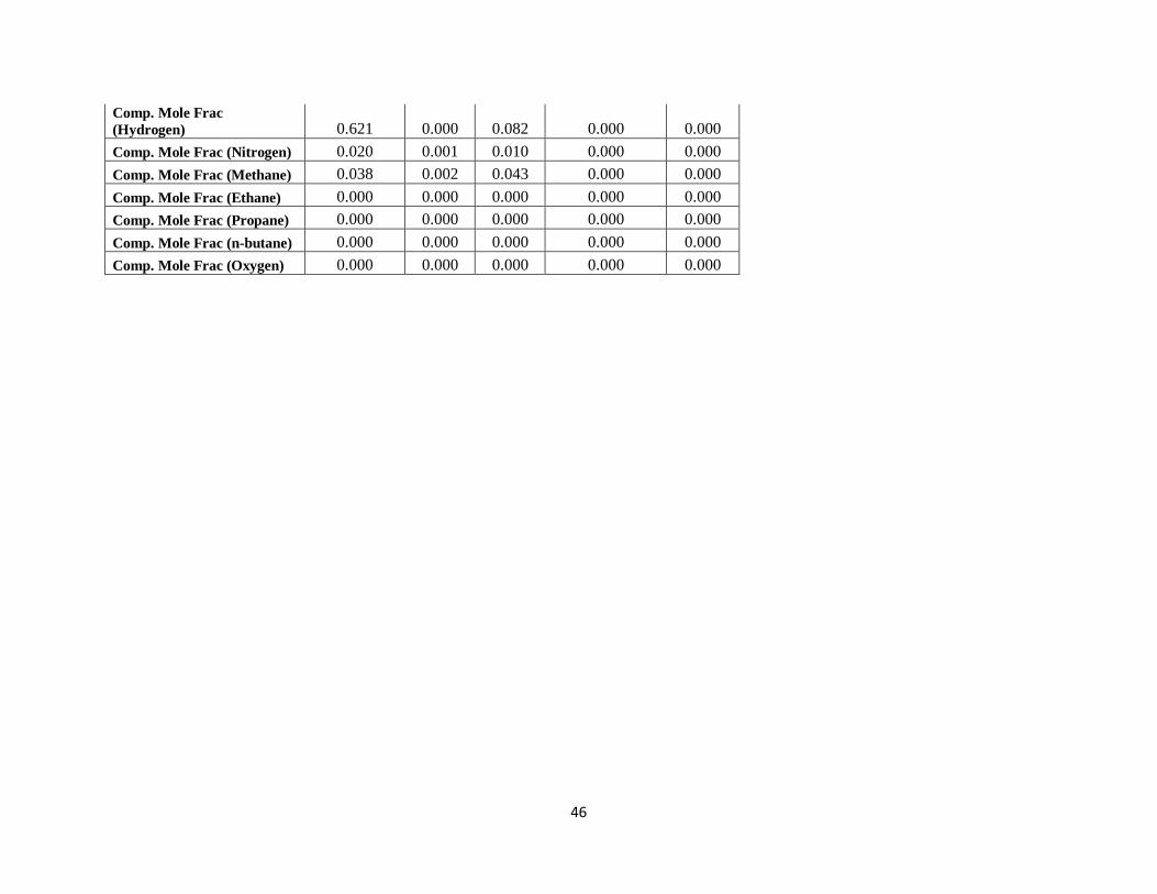
46

Comp. Mole Frac (Hydrogen) 0.621 0.000 0.082 0.000 0.000 Comp. Mole Frac (Nitrogen) 0.020 0.001 0.010 0.000 0.000 Comp. Mole Frac (Methane) 0.038 0.002 0.043 0.000 0.000 Comp. Mole Frac (Ethane) 0.000 0.000 0.000 0.000 0.000 Comp. Mole Frac (Propane) 0.000 0.000 0.000 0.000 0.000 Comp. Mole Frac (n-butane) 0.000 0.000 0.000 0.000 0.000 Comp. Mole Frac (Oxygen) 0.000 0.000 0.000 0.000 0.000

47

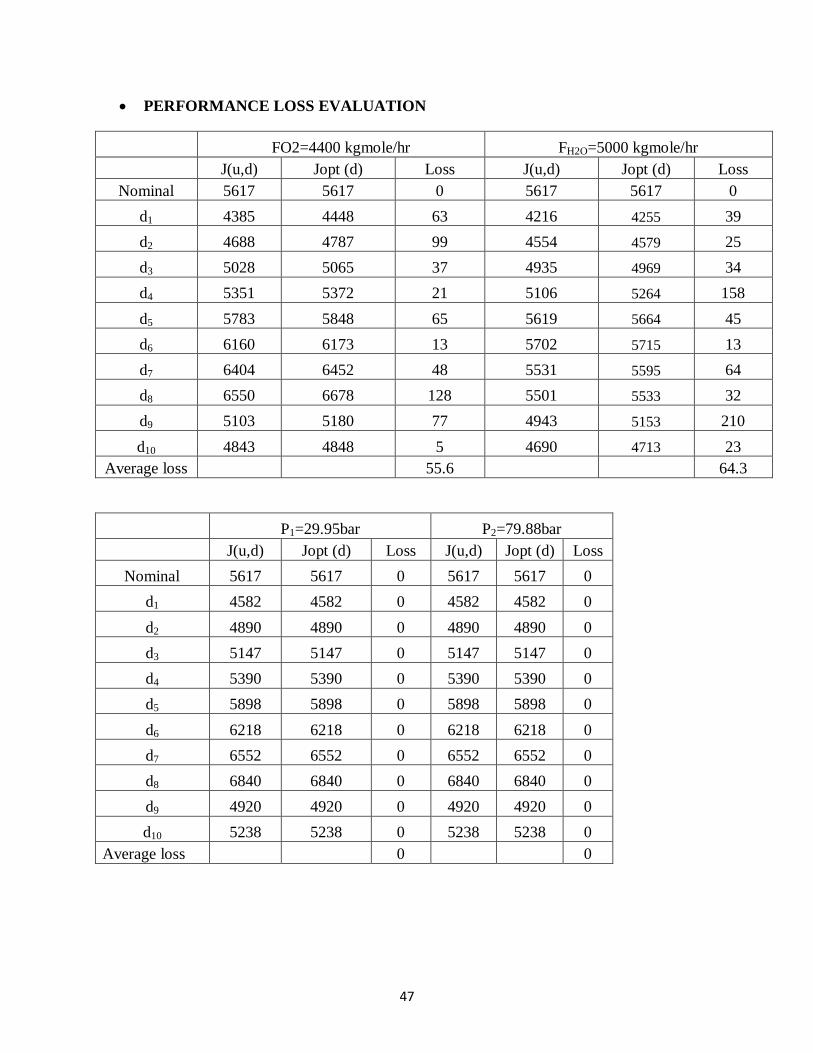
• PERFORMANCE LOSS EVALUATION

FO2=4400 kgmole/hr FH2O=5000 kgmole/hr J(u,d) Jopt (d) Loss J(u,d) Jopt (d) Loss

Nominal 5617 5617 0 5617 5617 0 d1 4385 4448 63 4216 4255 39 d2 4688 4787 99 4554 4579 25 d3 5028 5065 37 4935 4969 34 d4 5351 5372 21 5106 5264 158 d5 5783 5848 65 5619 5664 45 d6 6160 6173 13 5702 5715 13 d7 6404 6452 48 5531 5595 64 d8 6550 6678 128 5501 5533 32 d9 5103 5180 77 4943 5153 210 d10 4843 4848 5 4690 4713 23

Average loss 55.6 64.3

P1=29.95bar P2=79.88bar J(u,d) Jopt (d) Loss J(u,d) Jopt (d) Loss

Nominal 5617 5617 0 5617 5617 0 d1 4582 4582 0 4582 4582 0 d2 4890 4890 0 4890 4890 0 d3 5147 5147 0 5147 5147 0 d4 5390 5390 0 5390 5390 0 d5 5898 5898 0 5898 5898 0 d6 6218 6218 0 6218 6218 0 d7 6552 6552 0 6552 6552 0 d8 6840 6840 0 6840 6840 0 d9 4920 4920 0 4920 4920 0 d10 5238 5238 0 5238 5238 0

Average loss 0 0

48

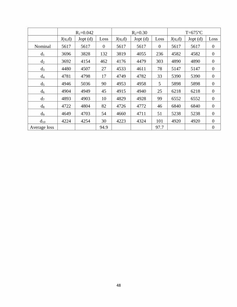
R1=0.042 R2=0.30 T=675°C J(u,d) Jopt (d) Loss J(u,d) Jopt (d) Loss J(u,d) Jopt (d) Loss

Nominal 5617 5617 0 5617 5617 0 5617 5617 0 d1 3696 3828 132 3819 4055 236 4582 4582 0 d2 3692 4154 462 4176 4479 303 4890 4890 0 d3 4480 4507 27 4533 4611 78 5147 5147 0 d4 4781 4798 17 4749 4782 33 5390 5390 0 d5 4946 5036 90 4953 4958 5 5898 5898 0 d6 4904 4949 45 4915 4940 25 6218 6218 0 d7 4893 4903 10 4829 4928 99 6552 6552 0 d8 4722 4804 82 4726 4772 46 6840 6840 0 d9 4649 4703 54 4660 4711 51 5238 5238 0 d10 4224 4254 30 4223 4324 101 4920 4920 0

Average loss 94.9 97.7 0

49

NOMENCLATURE Jopt(d) ................................................................................. J when re-optimizing the disturbance

L ............................................................................. Loss from optimum

d ............................................................................. Disturbance

CV .......................................................................... Control variable

MV ......................................................................... Manipulated variable

DoF ....................................................................... Degrees of freedom

u ......................................................................... Input

y ......................................................................... Output

∆H ........................................................................ Enthalpy of reaction [kJ/mol]

∆G ....................................................................... Gibbs Energy [kJ/mol]

∆S ....................................................................... Entropy, [J/Kmol]

B ........................................................................ Activation energy

R ......................................................................... Universal gas constant

A ......................................................................... Frequency factor for the reaction

Cp .................................................................... Specific heat of the gas constant pressure, [J/mol]

Di ............................................................. Tube inside diameter, [m]

fi .............................................................. Partial fugacity of component i, [bar]

F ............................................................. Total molar flowrate, [kgmole/hr]

k1 ........................................................... rate constant for1st rate equation of methanol synthesis reaction, [mol/kg s bar-1/2]

k2 ........................................................... rate constant for 2nd rate equation of methanol synthesis reaction, [mol/kg s bar-1/2]

k3 ........................................................... rate constant for 3rd rate equation of methanol synthesis reaction, [mol/kg s bar-1/2]

Ki .......................................................... Adsorption equilibrium constant for component i, bar-1

50

T ...................................................... Temperature, K

ρb ..................................................... Density of catalytic bed, [kg/m3]