539

Species distribution modelling as a macroecological tool: a case study using New World amphibians

Tiago S. Vasconcelos , Miguel Á . Rodr í guez and Bradford A. Hawkins

T. S. Vasconcelos (zoologia@ig.com.br) and B. A. Hawkins, Dept of Ecology and Evolutionary Biology, Univ. of California, Irvine, CA 92697, USA. – M. Á . Rodr í guez, Dept of Ecology, Univ. of Alcal á , Alcal á de Henares, ES-28871, Spain.

Although species distribution modelling (SDM) is widely accepted among the scientifi c community and is increasingly used in ecology, conservation biology and biogeography, methodological limitations generate potential problems for its application in macroecology. Using amphibian species richness in North and South America, we compare species richness patterns derived from SDM maps and ‘ expert ’ maps to evaluate if: 1) richness patterns derived from SDM are biased toward climate-based explanations for diversity when compared to expert maps, since SDM methods are typically based on climatic variables; and 2) SDM is a reliable tool for generating richness maps in hyperrich regions where point occurrence data are limited for many species. We found that although three widely used SDM methods overestimated amphibian species rich-ness in grid cells when compared to expert richness maps in both North and South America due to systematic overestimation of range sizes, diversity gradients were reasonably robust at broad scales. Further, climatic variables statistically explained patterns of richness at similar levels among the diff erent richness sources, although climatic relationships were stronger in the much better known North America than in South America. We conclude that in the face of the high deforestation rates coupled with incomplete data on species distributions, especially in the tropics, SDM represents a useful macroecological tool for investigating broad-scale richness patterns and the dynamics between species richness and climate.

Th e geographic distributions of species represent the basic units of macroecological analysis. For a few taxonomic groups, expert range maps now exist for most geographic areas and all known species, which have allowed the proliferation of macroecological studies performed at either the global scale (e.g. mammals: Sechrest 2003; birds: Hawkins et al. 2007; amphibians: Buckley and Jetz 2007) or over broad regions, such as Australia, Europe, and North America (Dijkstra and Lewington 2006, Montoya et al. 2007, Hawkins 2010). However, for most taxonomic groups, and particularly in the hyperdiverse tropics, range maps either do not exist or are very imprecise and incomplete, leaving us with the problem of how to conduct macroecological analyses in these situations.

An alternative to expert range maps is to approximate species ’ distributions with species distribution modelling (SDM) techniques (Elith and Burgman 2002, Guisan and Th uiller 2005, Elith et al. 2006), which associate species point occurrence and environmental data (generally precipi-tation and temperature, as well as more derived measures) at each occurrence point to generate a species distribution map. Although point data may be incomplete and geograph-ically biased, a wealth of occurrence records exists for many species and is becoming available on electronic databases. After being combined with digital environmental variables through some SDM method, new range maps can be gener-ated for those species for which expert maps are not avail-able. Subsequently, the distribution maps can be overlaid

and summed in a predefi ned point or grid system (hereafter SDM richness map) for studies of species richness patterns, as is usually done with range maps generated by expert opin-ion (hereafter expert richness map) (La Sorte and Hawkins 2007, Hawkins et al. 2008, Zafra-Calvo et al. 2010).

As SDM methods are generally based exclusively or primarily on climatic/productivity variables, and these vari-ables are known to have strong associations with broad-scale geographic patterns of species richness (Hawkins et al. 2003, Buckley and Jetz 2007, Field et al. 2009), distribution maps generated by SDM are widely accepted among the scientifi c community and are being increasingly used in a range of research fi elds (Franklin 2010). On the other hand, range maps generated by SDM are expected to overpredict the dis-tribution limits of species, predicting presence where it is known to be truly absent (errors of commission). Th is occurs because many SDM methods are unable to evaluate absences generated by species ’ evolutionary history, dispersal limita-tions, and biotic interactions with other species (Graham and Hijmans 2006, Pineda and Lobo 2009).

Methodological limitations of SDM methods generate potential problems for their application in macroecological analysis. One could argue that SDM richness maps, gener-ated by adding up individual SDM range maps of a given taxon in a pre-defi ned grid system, have stronger climatic relationships than richness maps generated by other species richness mapping methods, such as expert richness maps (Hawkins et al. 2008). So, because SDMs are commonly

Ecography 35: 539–548, 2012 doi: 10.1111/j.1600-0587.2011.07050.x

© 2011 Th e Authors. Ecography © 2011 Nordic Society Oikos Subject Editor: Catherine Graham. Accepted 1 July 2011

540

based on climatic variables, does it necessarily follow that SDM richness maps put too much emphasis on climate as a predictor of gradients? Th at is, if we generate a map of taxon richness for a group based on SDMs constructed using climate variables, would the richness pattern refl ect climatic variation more than the pattern identifi ed using less direct links between climate and richness (i.e. derived from range maps generated by experts on the group)? Th us, the fi rst aim of this study was to quantify the extent to which SDM richness maps overestimate links to climate relative to expert richness maps, using amphibians as a model sys-tem. Secondly, how well do SDM richness maps perform as sources of richness patterns when distribution data are lim-ited, as will often be the case in the tropics? In the absence of expert maps, range maps derived from SDMs may be the only ones available for most taxonomic groups in South America, Africa or Asia, as well as for many groups in North America, Europe and Australia, and evaluations of their ability to generate sensible geographic richness patterns are needed. To answer this question, we compared results for North America north of Mexico, which harbors relatively few well sampled amphibian species, and South America, where many more species occur and with expert range maps available for most of them, but simultaneously with far fewer point data for most species.

Methods

Point occurrence data and expert range maps

Point occurrence records for North and South American amphibians were obtained from three sources that provide open access to occurrence data from biological surveys and museum collections: the Global Biodiversity Information Facility (GBIF: � www.gbif.org � ; Yesson et al. 2007), HerpNET ( � www.herpnet.org � ), and SpeciesLink ( � http://splink.cria.org.br � ) databases. All records were carefully examined for probable errors, and the nomencla-ture of species was checked for synonymies and updated according to the American Museum of Natural History (AMNH) amphibian database (Frost 2010). We removed from our dataset all species with fewer than fi ve occurrence records, as well as introduced species (e.g. Lithobates catesbe-ianus and Xenopus laevis in South America). We also deleted nine species for which there were occurrence records but no expert range maps. Mexican records were included in the North American dataset when the species ’ range extended north of the Mexico – USA border. We were then able to gen-erate SDM range maps for 219 species in North America north of Mexico (with a total of 49 104 occurrence points) and 536 species in South America (with a total of 15 080 occurrence points) (Supplementary material Appendix 1 and 2). Finally, of the amphibian species currently recorded in the USA and Canada (296 species) and South America (2461 species) (AmphibiaWeb 2010), we obtained expert range maps for 268 and 2265 species, respectively, from the International Union for Conservation of Nature (IUCN) portal ( � www.iucnredlist.org/technical-documents/spatial-data � ). It is important to emphasize that the expert maps represent the areas where a particular species can be expected

to occur, although, within these areas, it will be found only in suitable habitats. Th us, overprediction is an inherent methodological limitation of these kinds of range maps (Graham and Hijmans 2006), although they may some-times function very well at grains greater than 50 � 50 km (Hawkins et al. 2008).

Species distribution modelling

We generated three sets of modeled ranges based on one bioclimatic envelope method (BIOCLIM) and two machine learning methods (OM-GARP and MAXENT). BIOCLIM characterizes sites that are located within the environ-mental hyper-space occupied by a species, in which the potential climatic domain is the multidimensional enve-lope that encompasses all recorded locations of the species (Nix 1986). OM-GARP is a version of GARP (Anderson et al. 2003) implemented in openModeller software (Mu ñ oz et al. 2011), which uses a genetic algorithm to select a set of rules that best predicts the species ’ distributions (Stockwell and Peters 1999). MAXENT estimates species ’ distributions by fi nding the distribution of maximum entropy (i.e. clos-est to uniform) subject to the constraint that the expected value of each environmental variable (or its transform and/or interactions) under this estimated distribution matches its empirical average (Phillips et al. 2006). BIOCLIM uses only presence data for model building, whereas OM-GARP and MAXENT use both presence and pseudoabsence data randomly sampled from the calibration area. For MAXENT, we entered 25% of the sample records as ‘ random test per-centage ’ , which means that the program randomly set aside 25% of the records for testing, i.e. 75% of the dataset was used for calibration (training) and the remaining 25% used for model evaluation (testing).

All three modelling methods are widely used and are known to have reasonable performance, but MAXENT tends to outperform OM-GARP, which in turn tends to outper-form BIOCLIM (Elith et al. 2006, Giovanelli et al. 2010). It is important to emphasize that despite the growing litera-ture generating methodological improvements in SDM (e.g. model assessment with a small number of occurrence records: Pearson et al. 2007) and the infl uence of large calibration areas (Giovanelli et al. 2010), we performed all modelling methods with the same set up and calibration areas (one for northern North America and one for South America). We adopted this procedure because the large number of species is better suited to a standardized procedure than to a species-by-species treatment that would be logistically complex and diffi cult to interpret. BIOCLIM and OM-GARP maps were generated in the openModeller 1.1.0 with default settings (Mu ñ oz et al. 2011; available at � http://openmodeller.sourceforge.net/ � ), whereas MAXENT maps were gener-ated in MAXENT 3.3.2, also with default settings (Phillips et al. 2006; available at � www.cs.princeton.edu/ ∼ schapire/maxent/ � ), but we deselected the option ‘ extrapolate ’ , in order to accept results only in areas where environmen-tal conditions fall within the range of the calibration area (Giovanelli et al. 2008, Th om é et al. 2010).

Th e environmental variables used to model species dis-tributions were selected to describe general climatic trends

541

(i.e. mean values), variation in temperature and precipitation over time, and potential physiological limits for amphibians (Nix 1986). Specifi cally, we used the following seven cli-matic variables, obtained from the WorldClim database at a spatial resolution of 10 km (Hijmans et al. 2005): annual mean temperature, temperature seasonality, minimum tem-perature of the coldest month, temperature annual range, annual precipitation, precipitation seasonality, and precipi-tation of the warmest quarter.

Th e SDM of each species was evaluated by the receiver operating characteristic (ROC) curve, a threshold-indepen-dent method that plots the true positive against the false pos-itive fractions of occurrence over a large range of thresholds (Elith and Burgman 2002). Th e area under the curve (AUC) is an important summary statistic for ROC plots, which ranges from 0 to 1. A value up to 0.5 implies no discrimina-tion, equivalent to random predictions. AUC values of 0.75 or above are generally considered suffi ciently discriminatory to be helpful (Elith and Burgman 2002).

To create the fi nal species richness maps, we generated binary predictive maps for each SDM method using thres-hold values. Diff erent approaches have been employed for setting thresholds (Liu et al. 2005), but most techniques depend on balancing false-positive and false-negative pre-dictions, applicable only when absence data are available (Pearson et al. 2007), which is not the case here. Although no general rule has been developed for diff erent algorithms (Phillips et al. 2006), we attempted to establish threshold values that balance commission and omission errors, i.e. the fi nal maps are supposed to be neither under nor over-represented. Th us, BIOCLIM binary maps were gener-ated considering marginal areas (threshold value of 50% in openModeller settings: Mu ñ oz et al. 2011). For OM-GARP maps, after an initial fi lter that removes very large and very small predictions from consideration (see details in Peterson et al. 2008), the resulting best subsets models are summed to produce a best ensemble estimate of geographic projection. Finally, openModeller generates the fi nal distribution binary range map, using the threshold percentage of 70% (default setting). MAXENT binary maps were generated using a threshold of 10, i.e. rejecting the lowest 10% of possible predicted values. Th is fi xed cumulative value at 10% can be considered a less conservative threshold when compared to others (e.g. minimum training presence) and maximizes the agreement between observed and predicted distributions (Phillips et al. 2006, Pearson et al. 2007, Milanovich et al. 2010).

As we used continental calibration areas for the SDMs, the diff erent modelling methods generated patchy potential distributions with large gaps throughout either North or South America for some species, which are unrealistic under most biologically plausible scenarios. Rather, these are envi-ronmentally suitable areas of a given species instead of pre-dicted distributions. Th e most common examples include 1) North American species occurring on either the east or west coast with isolated predicted areas on the opposite coast; and 2) South American species endemic to the Atlantic Rainforest (east coast) with isolated predicted areas in the Amazon forest. Both of these predictions are unrealistic, because colonization of widely separated patches will be limited by topography (e.g. the Rocky Mountains in north) or by the

absence of a climatically suitable region between discon-nected suitable areas (e.g. Cerrado in the south). Because we were interested in neither unrealistic potential distributions nor in potential areas for colonization or introduction, we deleted isolated predicted distribution areas more than 400 km away from any known occurrence record of a species.

Species richness maps

Species richness maps were generated for each map source (expert, BIOCLIM, OM-GARP, and MAXENT) by sum-ming in ArcGIS the presence/absence maps in 27.5 � 27.5 km (for mapping) and 110 � 110 km (for statistical analy-sis) grids. For expert maps, we generated two richness maps: one based in all species for which range maps were available ( ‘ all ’ dataset), and another only with those species for which we generated SDM maps ( ‘ modelled ’ dataset).

Because the number of species varied between expert and SDM maps (primarily for South America: 536 species with SDM maps and 2265 species with expert maps), we per-formed a simple correlation between the ‘ all ’ and ‘ modelled ’ richness datasets, for North and South America separately. Th is allowed us to assess how much information on the over-all richness gradient was lost by removing species that could not be modelled. We also performed a series of correlations between expert and SDM richness maps to quantify the sim-ilarity of richness gradients.

Range size maps

All else being equal, richness maps based on SDMs will over-estimate absolute richness values due to the fact that range sizes are primarily or exclusively generated considering only climate (i.e. ignoring more diffi cult to measure factors like biotic interactions and/or evolutionary constraints), and as a result, will overestimate the extent of occurrence of some spe-cies. Although the extent to which ranges are overestimated in any particular study will be diffi cult to assess a priori, when it does occur these regions are likely to have spatial structure, since the ranges of montane and other narrowly distributed species will probably be overestimated to a greater extent than broadly distributed species mostly found in lowlands. To explore how well the modelling methods compare to expert maps with respect to identifying geographic range size pat-terns, a second metric of wide interest to macroecologists, we generated and mapped mean log 10 range sizes in each cell.

Selection of climate models of amphibian richness

To evaluate links between environmental variables and amphibian species richness in North and South America, we extracted for each cell the values of the seven environ-mental variables used for modeling species distributions (see above), as well as standard deviation of elevation, which is a measure of topographic heterogeneity (elevation data available at � www.ngdc.noaa.gov/ecosys/cdroms/ged_iia/datasets/a13/fnoc.htm � ); and annual actual evapotranspi-ration (AET), a measure of water-energy balance (available at � http://gcmd.gsfc.nasa.gov � ).

542

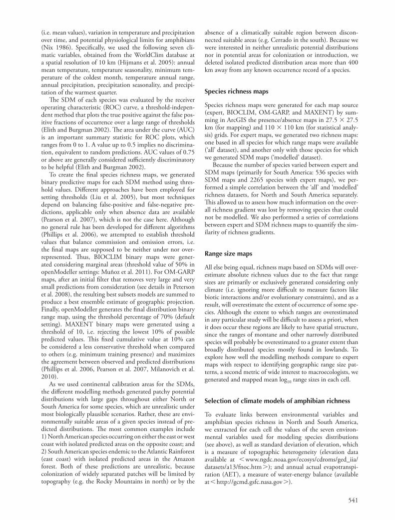
0.97 � 0.052 (BIOCLIM), 0.98 � 0.031 (OM-GARP) and 0.98 � 0.019 (MAXENT). In South America, all mean AUC values were 0.96 ( � 0.066 for BIOCLIM, � 0.056 for OM-GARP and � 0.046 for MAXENT). Th e species richness patterns identifi ed by the expert maps using the ‘ all ’ and ‘ modelled ’ datasets were almost perfectly associated in North America (r � 0.998) (Fig. 1a, b) and very similar in South America (r � 0.953) (Fig. 2a, b), although maxi-mum richness was necessarily lower when based on the sub-sets of species for which there were suffi cient numbers of records for modelling (i.e. the ‘ modelled ’ data set). Patterns of species richness predicted by expert vs SDM maps were also correlated in both continents, but more strongly in North America (ranging from r EXPERT � OM-GARP � 0.865 to r EXPERT � BIOCLIM � 0.919) (Fig. 1) than in South America (r EXPERT � OM-GARP � 0.621 to r EXPERT � BIOCLIM � 0.758) (Fig. 2).

As refl ected by the strong correlations among species richness estimates in North America, the richness patterns generated by both expert and SDM maps identifi ed the southeast as broadly supporting the most species (Fig. 1). However, some diff erences were found among the expert and SDM maps regarding smaller-scale distributions of richness within this region (Fig. 1), and all modeling methods over-estimated maximum richness relative to expert-map based estimates, MAXENT in particular (cf. Fig. 1b, e). All three SDM methods also overpredicted richness in the mountain-ous west, especially in the coastal ranges, Cascades and the Sierra Nevada (Fig. 1 and Supplementary material Appendix 3, Fig. A3). On the other hand, correlations between spe-cies-level range size estimates for expert-map based ranges

Th e relationships between the environmental variables and patterns of amphibian species richness were examined by generating a series of ordinary least-squares (OLS) multiple regressions. Th e model selection approach was based on the lowest Akaike information criterion (AIC). Th is study was not designed to determine what combination of environmental variables are most strongly associated with species richness pat-terns of amphibians (Rodr í guez et al. 2005); rather we wanted to compare models including a range of environmental vari-ables for richness data derived from diff erent sources (expert based vs SDM based). Th us, we performed OLS regressions with two sets of environmental variables: 1) including the seven climatic variables used for modeling species distribu-tions, and 2) including climatic/productivity and topographic variables that are known to be strong correlates for a wide range of plant and animal groups (Hawkins et al. 2003, Field et al. 2009). In addition, we examined two sets of response variables ( ‘ all ’ and ‘ modelled ’ datasets), to determine if the richness data-set containing all species ( ‘ all ’ dataset) results in substantially diff erent models than the richness dataset containing only the species included in the SDM ( ‘ modelled ’ dataset). Th en, com-bining the two sets of explanatory and the two sets of response variables, four sets of regression models were generated in each continent. Th e regressions were run in spatial analysis in mac-roecology (SAM) ver. 4.0 (Rangel et al. 2010).

Results

All three modelling methods had strong predictive power, with mean AUC � SD values in North America of

Figure 1. Geographical patterns of amphibian species richness in North America north of Mexico for (a) expert maps ( ‘ all ’ dataset), (b) expert maps ( ‘ modelled ’ dataset), (c) BIOCLIM maps, (d) OM-GARP maps, and (e) MAXENT maps. Data resolved to 27.5 � 27.5 km grain. Th e SDM maps include only those species in the ‘ modeled ’ expert dataset.

543

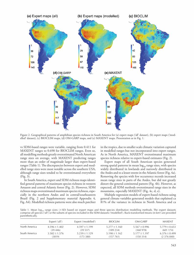
in the tropics, due to smaller scale climatic variation captured in modelled ranges but not incorporated into expert ranges. As in North America, MAXENT overestimated maximum species richness relative to expert-based estimates (Fig. 2).

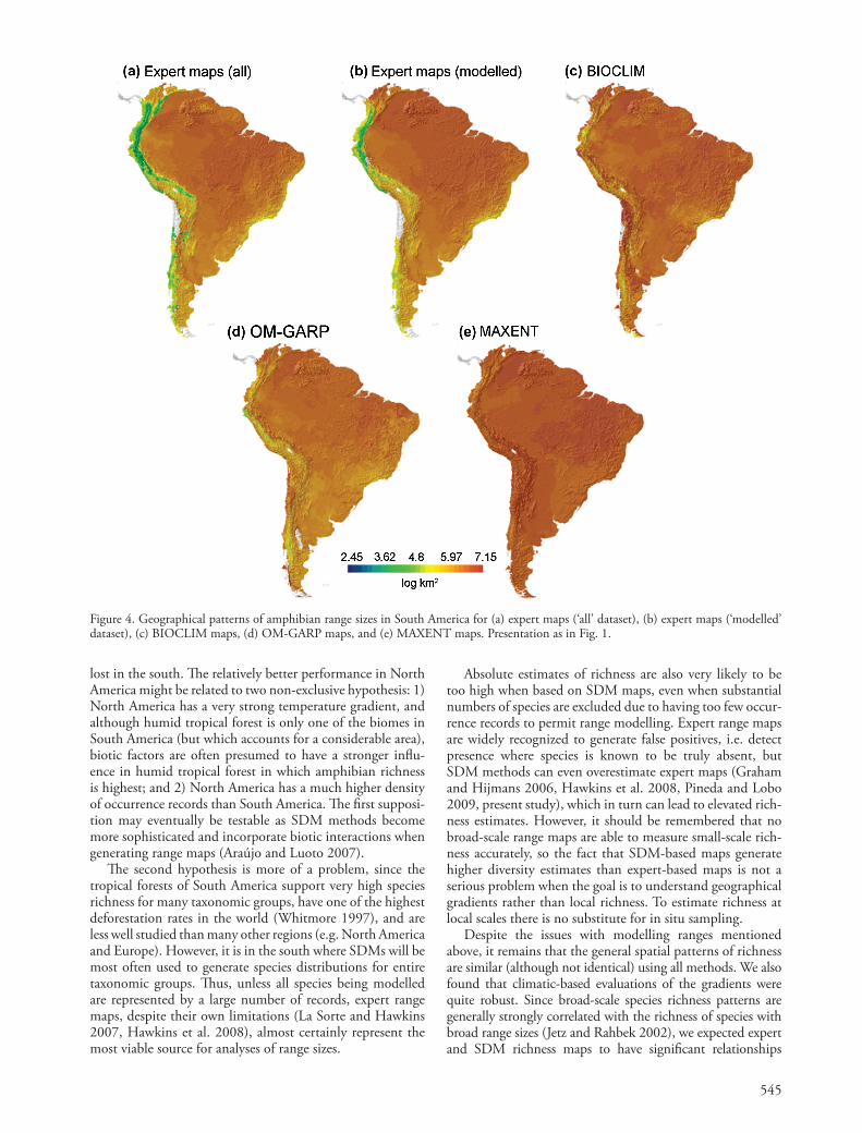
Expert maps of all South American species generated strong spatial patterns in mean log 10 range sizes, with species widely distributed in lowlands and narrowly distributed in the Andes and to a lesser extent in the Atlantic forest (Fig. 4a). Removing the species with few occurrence records increased mean range sizes in parts of the Andes, but did not greatly distort the general continental pattern (Fig. 4b). However, as expected, all SDM methods overestimated range sizes in the mountains, especially MAXENT (Fig. 4c, d, e).

Multiple regression models of expert-based richness using general climate variables generated models that explained ca 81% of the variance in richness in North America and ca

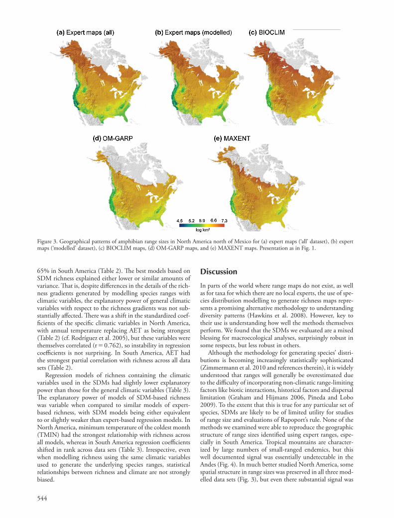
vs SDM-based ranges were variable, ranging from 0.411 for MAXENT ranges to 0.698 for BIOCLIM ranges. Even so, all modelling methods greatly overestimated North American range sizes on average, with MAXENT predicting ranges more than an order of magnitude larger than expert-based ranges (Table 1). Th e discrepancies between expert and mod-elled range sizes were most notable across the southern USA, although range sizes tended to be overestimated everywhere (Fig. 3).

In South America, expert and SDM richness maps identi-fi ed general patterns of maximum species richness in western Amazon and central Atlantic forest (Fig. 2). However, SDM richness maps overestimated maximum species richness, espe -cially in the northern Andes and in central/southeastern Brazil (Fig. 2 and Supplementary material Appendix 4, Fig. A4). Modelled richness patterns were also much patchier

Figure 2. Geographical patterns of amphibian species richness in South America for (a) expert maps ( ‘ all ’ dataset), (b) expert maps ( ‘ mod-elled ’ dataset), (c) BIOCLIM maps, (d) OM-GARP maps, and (e) MAXENT maps. Presentation as in Fig. 1.

Table 1. Mean log 10 range sizes ( � SD) based on expert maps and three species distribution modelling methods. The expert datasets comprise all species ( ‘ all ’ ) or the subsets of species included in the SDM datasets ( ‘ modelled ’ ). Back-transformed means (in km 2 ) are provided parenthetically.

Expert ( ‘ all ’ ) Expert ( ‘ modelled ’ ) BIOCLIM OM-GARP MAXENT

North America 4.596 � 1.402 4.597 � 1.199 5.277 � 1.160 5.567 � 0.996 5.779 � 0.653(39 446) (39 537) (189 234) (368 978) (601 174)

South America 3.582 � 1.576 5.239 � 1.129 5.198 � 1.162 5.177 � 1.197 6.376 � 0.499(3819) (173 380) (157 761) (150 314) (2 376 840)

544

Discussion

In parts of the world where range maps do not exist, as well as for taxa for which there are no local experts, the use of spe-cies distribution modelling to generate richness maps repre-sents a promising alternative methodology to understanding diversity patterns (Hawkins et al. 2008). However, key to their use is understanding how well the methods themselves perform. We found that the SDMs we evaluated are a mixed blessing for macroecological analyses, surprisingly robust in some respects, but less robust in others.

Although the methodology for generating species ’ distri-butions is becoming increasingly statistically sophisticated (Zimmermann et al. 2010 and references therein), it is widely understood that ranges will generally be overestimated due to the diffi culty of incorporating non-climatic range-limiting factors like biotic interactions, historical factors and dispersal limitation (Graham and Hijmans 2006, Pineda and Lobo 2009). To the extent that this is true for any particular set of species, SDMs are likely to be of limited utility for studies of range size and evaluations of Rapoport ’ s rule. None of the methods we examined were able to reproduce the geographic structure of range sizes identifi ed using expert ranges, espe-cially in South America. Tropical mountains are character-ized by large numbers of small-ranged endemics, but this well documented signal was essentially undetectable in the Andes (Fig. 4). In much better studied North America, some spatial structure in range sizes was preserved in all three mod-elled data sets (Fig. 3), but even there substantial signal was

Figure 3. Geographical patterns of amphibian range sizes in North America north of Mexico for (a) expert maps ( ‘ all ’ dataset), (b) expert maps ( ‘ modelled ’ dataset), (c) BIOCLIM maps, (d) OM-GARP maps, and (e) MAXENT maps. Presentation as in Fig. 1.

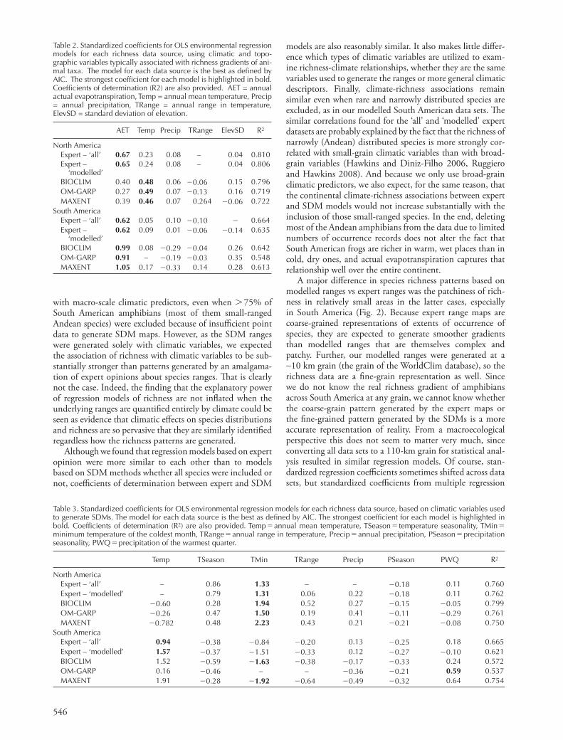
65% in South America (Table 2). Th e best models based on SDM richness explained either lower or similar amounts of variance. Th at is, despite diff erences in the details of the rich-ness gradients generated by modelling species ranges with climatic variables, the explanatory power of general climatic variables with respect to the richness gradients was not sub-stantially aff ected. Th ere was a shift in the standardized coef-fi cients of the specifi c climatic variables in North America, with annual temperature replacing AET as being strongest (Table 2) (cf. Rodr í guez et al. 2005), but these variables were themselves correlated (r � 0.762), so instability in regression coeffi cients is not surprising. In South America, AET had the strongest partial correlation with richness across all data sets (Table 2).

Regression models of richness containing the climatic variables used in the SDMs had slightly lower explanatory power than those for the general climatic variables (Table 3). Th e explanatory power of models of SDM-based richness was variable when compared to similar models of expert-based richness, with SDM models being either equivalent to or slightly weaker than expert-based regression models. In North America, minimum temperature of the coldest month (TMIN) had the strongest relationship with richness across all models, whereas in South America regression coeffi cients shifted in rank across data sets (Table 3). Irrespective, even when modelling richness using the same climatic variables used to generate the underlying species ranges, statistical relationships between richness and climate are not strongly biased.

545

lost in the south. Th e relatively better performance in North America might be related to two non-exclusive hypothesis: 1) North America has a very strong temperature gradient, and although humid tropical forest is only one of the biomes in South America (but which accounts for a considerable area), biotic factors are often presumed to have a stronger infl u-ence in humid tropical forest in which amphibian richness is highest; and 2) North America has a much higher density of occurrence records than South America. Th e fi rst supposi-tion may eventually be testable as SDM methods become more sophisticated and incorporate biotic interactions when generating range maps (Ara ú jo and Luoto 2007).

Th e second hypothesis is more of a problem, since the tropical forests of South America support very high species richness for many taxonomic groups, have one of the highest deforestation rates in the world (Whitmore 1997), and are less well studied than many other regions (e.g. North America and Europe). However, it is in the south where SDMs will be most often used to generate species distributions for entire taxonomic groups. Th us, unless all species being modelled are represented by a large number of records, expert range maps, despite their own limitations (La Sorte and Hawkins 2007, Hawkins et al. 2008), almost certainly represent the most viable source for analyses of range sizes.

Figure 4. Geographical patterns of amphibian range sizes in South America for (a) expert maps ( ‘ all ’ dataset), (b) expert maps ( ‘ modelled ’ dataset), (c) BIOCLIM maps, (d) OM-GARP maps, and (e) MAXENT maps. Presentation as in Fig. 1.

Absolute estimates of richness are also very likely to be too high when based on SDM maps, even when substantial numbers of species are excluded due to having too few occur-rence records to permit range modelling. Expert range maps are widely recognized to generate false positives, i.e. detect presence where species is known to be truly absent, but SDM methods can even overestimate expert maps (Graham and Hijmans 2006, Hawkins et al. 2008, Pineda and Lobo 2009, present study), which in turn can lead to elevated rich-ness estimates. However, it should be remembered that no broad-scale range maps are able to measure small-scale rich-ness accurately, so the fact that SDM-based maps generate higher diversity estimates than expert-based maps is not a serious problem when the goal is to understand geographical gradients rather than local richness. To estimate richness at local scales there is no substitute for in situ sampling.

Despite the issues with modelling ranges mentioned above, it remains that the general spatial patterns of richness are similar (although not identical) using all methods. We also found that climatic-based evaluations of the gradients were quite robust. Since broad-scale species richness patterns are generally strongly correlated with the richness of species with broad range sizes (Jetz and Rahbek 2002), we expected expert and SDM richness maps to have signifi cant relationships

546

Table 3. Standardized coeffi cients for OLS environmental regression models for each richness data source, based on climatic variables used to generate SDMs. The model for each data source is the best as defi ned by AIC. The strongest coeffi cient for each model is highlighted in bold. Coeffi cients of determination (R 2 ) are also provided. Temp � annual mean temperature, TSeason � temperature seasonality, TMin � minimum temperature of the coldest month, TRange � annual range in temperature, Precip � annual precipitation, PSeason � precipitation seasonality, PWQ � precipitation of the warmest quarter.

Temp TSeason TMin TRange Precip PSeason PWQ R 2

North AmericaExpert – ‘ all ’ – 0.86 1.33 – – �0.18 0.11 0.760Expert – ‘ modelled ’ – 0.79 1.31 0.06 0.22 �0.18 0.11 0.762BIOCLIM �0.60 0.28 1.94 0.52 0.27 �0.15 �0.05 0.799OM-GARP �0.26 0.47 1.50 0.19 0.41 �0.11 �0.29 0.761MAXENT �0.782 0.48 2.23 0.43 0.21 �0.21 �0.08 0.750

South AmericaExpert – ‘ all ’ 0.94 �0.38 �0.84 �0.20 0.13 �0.25 0.18 0.665Expert – ‘ modelled ’ 1.57 �0.37 �1.51 �0.33 0.12 �0.27 �0.10 0.621BIOCLIM 1.52 �0.59 �1.63 �0.38 �0.17 �0.33 0.24 0.572OM-GARP 0.16 �0.46 – – �0.36 �0.21 0.59 0.537MAXENT 1.91 �0.28 �1.92 �0.64 �0.49 �0.32 0.64 0.754

Table 2. Standardized coeffi cients for OLS environmental regression models for each richness data source, using climatic and topo-graphic variables typically associated with richness gradients of ani-mal taxa. The model for each data source is the best as defi ned by AIC. The strongest coeffi cient for each model is highlighted in bold. Coeffi cients of determination (R2) are also provided. AET = annual actual evapotranspiration, Temp = annual mean temperature, Precip = annual precipitation, TRange = annual range in temperature, ElevSD = standard deviation of elevation.

AET Temp Precip TRange ElevSD R 2

North AmericaExpert – ‘ all ’ 0.67 0.23 0.08 – 0.04 0.810Expert –

‘ modelled ’ 0.65 0.24 0.08 – 0.04 0.806

BIOCLIM 0.40 0.48 0.06 �0.06 0.15 0.796OM-GARP 0.27 0.49 0.07 �0.13 0.16 0.719MAXENT 0.39 0.46 0.07 0.264 �0.06 0.722

South America Expert – ‘ all ’ 0.62 0.05 0.10 �0.10 � 0.664Expert –

‘ modelled ’ 0.62 0.09 0.01 �0.06 �0.14 0.635

BIOCLIM 0.99 0.08 �0.29 �0.04 0.26 0.642OM-GARP 0.91 – �0.19 �0.03 0.35 0.548MAXENT 1.05 0.17 �0.33 0.14 0.28 0.613

with macro-scale climatic predictors, even when � 75% of South American amphibians (most of them small-ranged Andean species) were excluded because of insuffi cient point data to generate SDM maps. However, as the SDM ranges were generated solely with climatic variables, we expected the association of richness with climatic variables to be sub-stantially stronger than patterns generated by an amalgama-tion of expert opinions about species ranges. Th at is clearly not the case. Indeed, the fi nding that the explanatory power of regression models of richness are not infl ated when the underlying ranges are quantifi ed entirely by climate could be seen as evidence that climatic eff ects on species distributions and richness are so pervasive that they are similarly identifi ed regardless how the richness patterns are generated.

Although we found that regression models based on expert opinion were more similar to each other than to models based on SDM methods whether all species were included or not, coeffi cients of determination between expert and SDM

models are also reasonably similar. It also makes little diff er-ence which types of climatic variables are utilized to exam-ine richness-climate relationships, whether they are the same variables used to generate the ranges or more general climatic descriptors. Finally, climate-richness associations remain similar even when rare and narrowly distributed species are excluded, as in our modelled South American data sets. Th e similar correlations found for the ‘ all ’ and ‘ modelled ’ expert datasets are probably explained by the fact that the richness of narrowly (Andean) distributed species is more strongly cor-related with small-grain climatic variables than with broad-grain variables (Hawkins and Diniz-Filho 2006, Ruggiero and Hawkins 2008). And because we only use broad-grain climatic predictors, we also expect, for the same reason, that the continental climate-richness associations between expert and SDM models would not increase substantially with the inclusion of those small-ranged species. In the end, deleting most of the Andean amphibians from the data due to limited numbers of occurrence records does not alter the fact that South American frogs are richer in warm, wet places than in cold, dry ones, and actual evapotranspiration captures that relationship well over the entire continent.

A major diff erence in species richness patterns based on modelled ranges vs expert ranges was the patchiness of rich-ness in relatively small areas in the latter cases, especially in South America (Fig. 2). Because expert range maps are coarse-grained representations of extents of occurrence of species, they are expected to generate smoother gradients than modelled ranges that are themselves complex and patchy. Further, our modelled ranges were generated at a ∼ 10 km grain (the grain of the WorldClim database), so the richness data are a fi ne-grain representation as well. Since we do not know the real richness gradient of amphibians across South America at any grain, we cannot know whether the coarse-grain pattern generated by the expert maps or the fi ne-grained pattern generated by the SDMs is a more accurate representation of reality. From a macroecological perspective this does not seem to matter very much, since converting all data sets to a 110-km grain for statistical anal-ysis resulted in similar regression models. Of course, stan-dardized regression coeffi cients sometimes shifted across data sets, but standardized coeffi cients from multiple regression

547

Bini, L. M. et al. 2009. Coeffi cient shifts in geographical ecology: an empirical evaluation of spatial and non-spatial regression. – Ecography 32: 193 – 204.

Buckley, L. B. and Jetz, W. 2007. Environmental and historical constraints on global patterns of amphibian richness. – Proc. R. Soc. B 274: 1167 – 1173.

Dijkstra, K. B. and Lewington, R. 2006. Field guide to the drag-onfl ies of Britain and Europe. – British Wildlife Publishing.

Elith, J. and Burgman, M. 2002. Predictions and their validation: rare plants in the Central Highlands, Victoria, Australia. – In: Scott, J. M. et al. (eds), Predicting species occurrences: issues of accuracy and scale. Island Press, pp. 303 – 314.

Elith, J. et al. 2006. Novel methods improve prediction of species ’ distribution from occurrence data. – Ecography 29: 129 – 151.

Field, R. et al. 2009. Spatial species - richness gradients across scales: a meta - analysis. – J. Biogeogr. 36: 132 – 147.

Franklin, J. 2010. Mapping species distributions: spatial inference and prediction. – Cambridge Univ. Press.

Frost, D. R. 2010. Amphibian species of the world: an online reference. Version 5.4. – American Museum of Natural History, NY, USA, � http://research.amnh.org/vz/herpetology/amphibia/ � accessed 8 April 2010.

Giovanelli, J. G. R. et al. 2008. Predicting the potential distribu-tion of the alien invasive American bullfrog ( Lithobates catesbe-ianus ) in Brazil. – Biol. Invasions 10: 585 – 590.

Giovanelli, J. G. R. et al. 2010. Modeling a spatially restricted distribution in the Neotropics: how the size of calibration area aff ects the performance of fi ve presence - only methods. – Ecol. Model. 221: 215 – 224.

Graham, C. H. and Hijmans, R. J. 2006. A comparison of meth-ods for mapping species range and species richness. – Global Ecol. Biogeogr. 15: 578 – 587.

Guisan, A. and Th uiller, W. 2005. Predicting species distribution: off ering more than simple habitat models. – Ecol. Lett. 8: 993 – 1009.

Hawkins, B. A. 2010. Multiregional comparison of the ecological and phylogenetic structure of butterfl y species richness gradients. – J. Biogeogr. 37: 647 – 656.

Hawkins, B. A. and Diniz – Filho, J. A. F. 2006. Beyond Rapoport ’ s rule: evaluating range size patterns of New World birds in a two-dimensional framework. – Global Ecol. Biogeogr. 15: 461 – 469.

Hawkins, B. A. et al. 2003. Energy, water, and broad-scale geographic patterns of species richness. – Ecology 84: 3105 – 3117.

Hawkins, B. A. et al. 2007. Climate, niche conservatism, and the global bird diversity gradient. – Am. Nat. 170: S16 – S27.

Hawkins, B. A. et al. 2008. What do range maps and surveys tell us about diversity patterns? – Folia Geobot. 43: 345 – 355.

Hernandez, P. A. et al. 2006. Th e eff ect of sample size and species characteristics on performance of diff erent species distribution modeling methods. – Ecography 29: 773 – 785.

Hijmans, R. J. et al. 2005. Very high resolution interpolated climate surfaces for global land areas. – Int. J. Climatol. 25: 1965 – 1978.

Jetz, W. and Rahbek, C. 2002. Geographic range size and deter-minants of avian species richness. – Science 297: 1548 – 1555.

La Sorte, F. A. and Hawkins, B. A. 2007. Range maps and species richness patterns: errors of commission and estimates of uncer-tainty. – Ecography 30: 649 – 662.

Liu, C. et al. 2005. Selecting thresholds of occurrence in the predic-tion of species distributions. – Ecography 28: 385 – 393.

Mathias, P. V. C. et al. 2004. Sensitivity of macroecological patterns of South American parrots to diff erences in data sources. – Global Ecol. Biogeogr. 13: 193 – 198.

Meier, E. S. et al. 2010. Biotic and abiotic variables show little redundancy in explaining tree species distributions. – Ecography 33: 1038 – 1048.

models of richness patterns are unstable both in the face of the collinear predictor variables often included in climatic evaluations of diversity gradients and depending on which particular spatially explicit or OLS regression method is used (Bini et al. 2009). We did not conduct detailed evalu-ations of covariances among predictors because we were interested in knowing how well climate explains the rich-ness gradients derived from multiple sources, irrespective of what particular climatic variables have the strongest partial regression coeffi cients. Th erefore, the fact that coeffi cients sometimes change when diff erent richness data are used is not unusual and does not alter the main conclusion that the detection of statistical links between climate and rich-ness are surprisingly robust to the source of the data. Similar levels of robustness have also been detected when diff erent sources of expert maps are used to conduct macroecological analyses (Mathias et al. 2004).

In conclusion, we suggest that SDM methods are a useful tool for macroecological analysis when no other option is available. On the other hand, it is important to emphasize that no method is perfect. Care is needed when interpreting richness patterns generated from SDMs due to their inherent tendency to overestimate species richness while at the same time missing many montane species due to data availability (in our case, we were forced to ignore � 75% of amphibian species in South America). Th e former issue should become less of a problem as the methods become more sophisti-cated, and additional non-climatic variables are included in the modelling process (Ara ú jo and Luoto 2007, Meier et al. 2010, Pellissier et al. 2010), but generating complex distribu-tion models for an entire taxonomic group in the tropics that may comprise hundreds or thousands of species presents its own challenges. It may also eventually be possible to devise methods to model narrowly-distributed species even when there are few occurrence records (Hernandez et al. 2006, Pearson et al. 2007). Irrespective, in the presence of human impacts and rapid climate change we do not have the luxury of waiting for perfect methods and data, and even imperfect SDM maps appear to capture climate–richness relationships as well as do expert maps.

Acknowledgements – Th e authors are grateful to Jo ã o G. R. Giovanelli for discussion of modelling methods, and Renato De Giovanni for assistance with openModeller. TSV was supported by Funda ç ã o de Amparo à Pesquisa no Estado de S ã o Paulo, Brazil (FAPESP; grant: 2009/17195-3), and MAR by the Spanish Ministries of Education (sabbatical grant: PR2009-0107) and Science and Innovation (grant: CGL2010-22119).

References

AmphibiaWeb 2010. Information on amphibian biology and con-servation (web application). – Berkeley, CA, � http://amphib-iaweb.org/ � , accessed 2 Nov 2010.

Anderson, R. P. et al. 2003. Evaluating predictive models of species ’ distribution: criteria for selecting optimal models. – Ecol. Model. 162: 211 – 232.

Ara ú jo, M. B. and Luoto, M. 2007. Th e importance of biotic inter-actions for modelling species distributions under climate change. – Global Ecol. Biogeogr. 16: 743 – 753.

548

Rodr í guez, M. Á . et al. 2005. Energy, water and large-scale patterns of reptile and amphibian species richness in Europe. – Acta Oecol. 28: 65 – 70.

Ruggiero, A. and Hawkins, B. A. 2008. Why do mountains sup-port so many species of birds? – Ecography 31: 306 – 315.

Sechrest, W. W. 2003. Global diversity, endemism, and conserva-tion of mammals. – PhD thesis, Univ. Virginia, USA.

Stockwell, D. and Peters, D. 1999. Th e GARP modelling system: problems and solutions to automated spatial prediction. – Int. J. Geogr. Inf. Sci. 13: 143 – 158.

Th om é , M. T. C. et al. 2010. Phylogeography of endemic toads and post-Pliocene persistence of the Brazilian Atlantic Forest. – Mol. Phylogenet. Evol. 55: 1018 – 1031.

Whitmore, T. C. 1997. Tropical forest disturbance, disappearance, and species loss. – In: Laurance, W. F. and Bierregaard Jr, R. O. (eds), Tropical forest remnants: ecology, management, and conser-vation of fragmented communities. Univ. of Chicago Press, pp. 3 – 12.

Yesson, C. et al. 2007. How global is the global biodiversity infor-mation facility? – PloS One 11: 1 – 10.

Zafra-Calvo, N. et al. 2010. Deriving species richness, endemism, and threatened species patterns from incomplete distribution data in the Bioko island, Equatorial Guinea. – Nat. Con-serva ç ã o. 8: 27 – 33.

Zimmermann, N. E. et al. 2010. New trends in species distribution modelling. – Ecography 33: 985 – 989.

Milanovich, J. R. et al. 2010. Projected loss of salamander diversity hotspot as a consequence of projected global climate change. – PloS One 5: 1 – 10.

Montoya, D. et al. 2007. Contemporary richness of Holarctic trees and the historical pattern of glacial retreat. – Ecography 30: 173 – 182.

Mu ñ oz, M. E. S. et al. 2011. openModeller: a generic approach to species ’ potential distribution modelling. – Geoinformatica 15: 111 – 135.

Nix, H. A. 1986. A biogeographic analysis of Australian elapid snakes. – In: Longmore, R. (ed.), Atlas of Australian elapid snakes. Australian Flora and Fauna Series, pp. 4 – 15.

Pearson, R. G. et al. 2007. Predicting species distributions from small numbers of occurrence records: a test case using cryptic geckos in Madagascar. – J. Biogeogr. 34: 102 – 117.

Pellissier, L. et al. 2010. Species distribution models reveal apparent competitive and facilitative eff ects of a dominant species on the distribution of tundra plants. – Ecography 33: 1004 – 1014.

Peterson, A. T. et al. 2008. Shifting global invasive potential of European plants with climate change. – PloS One 3: 1 – 7.

Phillips, S. J. et al. 2006. Maximum entropy modeling of species geographic distributions. – Ecol. Model. 190: 231 – 259.

Pineda, E. and Lobo, J. M. 2009. Assessing the accuracy of species distribution models to predict amphibian species richness patterns. – J. Anim. Ecol. 78: 182 – 190.

Rangel, T. F. et al. 2010. SAM: a comprehensive application for spatial analysis in macroecology. – Ecography 33: 46–50.

Supplementary material (Appendix E7050 at � www.oikosoffi ce.lu.se/appendix � ). Appendix 1 – 4.