Specification of surface figure and finish in terms of system performance

Specification of surface figureand finish in terms of system performance

E. L. Church and P. Z. Takacs

We describe methods of predicting the degradation of the performance of a simple imaging system interms of the statistics of the shape errors of the focusing element and, conversely, of specifying thosestatistics in terms of requirements on image quality. Results are illustrated for normal-incidence, x-raymirrors with figure errors plus conventional and/or fractal finish errors. It is emphasized that theimaging properties of a surface with fractal errors are well behaved even though fractal-power spectradiverge at low spatial frequencies.

Key words: X-ray imaging, surface scattering, surface finish, surface figure, fractal surfaces, surfacespecification.

1. IntroductionBrookhaven National Laboratory is the site of theNational Synchrotron Light Source, an electron syn-chrotron that is an intense source of hard and soft xrays. Since there are no effective refracting ele-ments for x rays, this radiation must be manipulatedand focused by mirrors configured to give high reflec-tivity.

In the case of hard x rays this is done with high-Zmetal mirrors illuminated at glancing angles of inci-dence below the critical angle for total externalreflection. Most synchrotron mirrors and high-energy x-ray telescopes use this method. In the caseof soft x rays, reasonable normal-incidence reflectiv-ity can be achieved with multilayer interferencecoatings.

There are two further differences between x-rayand conventional optics resulting from the shortradiation wavelengths involved: The image qualityis more sensitive to shape errors in the opticalelements, and, even in the case of a perfectly shapedmirror, the image is generally system rather thandiffraction limited.

Several years ago we developed a simple diffractiontheory for the imaging of glancing-incidence x-raymirrors that we called the five-factor formula; itrelated the image quality of system-limited optics to

E. L. Church is with USA ARDEC, Picatinny Arsenal, NewJersey 07806-5000. P. Z. Takacs is with the Brookhaven NationalLaboratory, Upton, New York 11973-5000.

Received 11 November 1992.0003-6935/93/3344-10$06.00/0.3 1993 Optical Society of America.

the statistics of the errors in the mirror shape.' Inthis paper we describe the generalization of thoseresults to normal-incidence optics. 2 3

Although we discuss this method with reference toshape errors in x-ray mirrors, the formalism is alsoapplicable to other sources of wave-front errors, toarbitrary radiation wavelengths, and to refractiveoptics.

2. Diffraction Theory of ImagingTo display the physics involved most clearly, weconsider the paraxial imaging of an on-axis parabolicmirror with statistically symmetric shape errors.The object is to develop simple relationships betweenshape errors and image quality and, conversely, tospecify limits on the statistics of those errors in termsof performance requirements.

The diffraction expression for the measured angu-lar distribution of the reflected and scattered inten-sity in the image plane is given by

1 dI 1 C1(0) = de A= J dT exp(i27rf * T)OTF(T), (1)

where

I(o) is the measured intensity distribution orspread function in the image plane as a function ofthe deflection angles 0, including both system effectsand surface-shape errors. It is normalized so thatintegration over all angles gives unity.

Is(0) is the corresponding expression for thesystem spread function, i.e., the image-intensity dis-tribution for zero surface errors.

3344 APPLIED OPTICS / Vol. 32, No. 19 / 1 July 1993

Ii is the total incident intensity.R is the normal-incidence intensity-reflection

coefficient.do is the solid angle element.X is the radiation wavelength.i is the lag vector in the surface plane, which is

related to the spatial-frequency vector in the imageplane g, through g = r/ XF, where F is the focaldistance.

f is the spatial frequency in the mirror plane,which is related to the image directions 0 and (p by thenormal-incidence form of the vector grating equation:

f(= ) = A(csn ) C p (2)

OTF () is the total optical transfer function ofthe system, normalized to unity at zero lag.

The total OTF is the product of two factors:

OTF(T) = OTF,() X OTFe,(). (3)

The first accounts for system effects and the secondfor the surface errors. For a perfectly shaped sur-face, OTFe(T) = 1, and Eq. (1) gives the system spreadfunction Is(o). The system and error OTF factorsare discussed in detail in the next two sections.

3. System OTFThe system factor in the total OTF can be written asthe product of three subfactors:

OTF8QT) = A1 (T) x A2(r) x A3(r), (4)

which account for illumination, source, and detectoreffects, as described below.

A. Illumination FactorAl is the illumination factor, which is the autocorrela-tion of the pupil function. For a simple circularpupil of diameter Do

Al(r) =- arccos( -) - - (-) 1|/ (5)

which, taken alone, leads to the well-known Airydistribution for the image intensity:

'T ~r D\ 2 il(n.DoO/ X) ]2I1() = - ) [ DO /2X 1 (6)

B. Source-Size FactorA2 is the source-size factor. In the case of x rays thesource is modeled as a collection of incoherent pointsources with a Gaussian angular distribution withthe rms angular width O,. The source-size factor isthen

A2(') = exp[-('OST/ X) 2 ], (7)

which corresponds to the intensity distribution

I2(O) = -i exp[-(0/08 )2 ]. (8)

C. Detector-Size FactorA 3 is the detector-size factor. In the case of acylindrical detector response with an angular diame-ter OD, it has the sombrero-function form

A 3(T) = (OW/2 X (9)

and the corresponding measured intensity distribu-tion is

413(0) = 4 CYI(0/OD), (10)

where Cyl(x) = 1 for Ix < 1/2 and zero otherwise.

D. Form of the System Spread FunctionThe fact that Eq. (4) is in the form of a product meansthat the system spread function is the triple convolu-tion of the intensity distributions given in Eqs. (6),(8), and (10):

IS(o) = Il(O) * 2(O) * I3(0)- (11)

Each term and its convolution have a unit volume,corresponding to the fact that each A and theirproduct are unity at zero lag. These unit propertiesare statements of the conservation of energy.

The analytic form of the system spread functionderived in this way is complicated. In this paper,however, we are less interested in the form of thatfunction than in how it is modified by the presence ofsurface errors. For that purpose we choose a simpleGaussian form for the system OTF:

OTFQT) = exp[-(Qwr/W) 2 ], (12)

where W is a length parameter characterizing thewidth of the system OTF, which we call the coherencelength on the surface of the optic.

The corresponding form for the system spreadfunction is

Is(o) =- )exp[-(W0/)2], (13)

which has the rms width:

width Is(o) =- A 00. (14)

E. System-Limited OpticsThe relative importance of the three terms in Eq. (11)depends on the radiation wavelength; the width of theillumination term I, is proportional to X, while I2 and13 are independent of X. This means that the illumi-nation term dominates at long wavelengths, while the

1 July 1993 / Vol. 32, No. 19 / APPLIED OPTICS 3345

others dominate at short wavelengths. In otherwords, visible-light optics may be diffraction limited,but x-ray optics tend to be system limited.3

For example, a 10-cm-diameter mirror imaging140-A (14-nm) radiation has a diffraction width of theorder of a tenth of a microradian, compared withtypical source-detector widths of tens or hundreds ofmicroradians.

Equation (14) shows this in a different way. In thediffraction-limited case the coherence length W is aconstant equal to the diameter of the focusing ele-ment, and the image width is proportional to X. Inthe system-limited case, on the other hand, the imagewidth is a constant, and it is the coherence length,which is now smaller than the diameter of the mirror,that is proportional to X.

If the system described above has a combinedsource-detector diameter of 100 rad (21 arcsec), Wis only 0.140 mm. Halving X halves W.

4. Error OTF

A. Relationship to the Surface-Structure FunctionThe second factor in the total OTF, OTFe, accountsfor the effects of the phase modulation introducedinto the reflected wave front by the shape errors inthe mirror surface. If those errors are members ofGaussian random processes,

OTFe(T) = exp[- - - D(T)] (15)

where D(T) is the structure function of the shapeerrors Z(X),4

D(T) = ([Z(X + T) - Z(X)]2). (16)

Here x is the position vector in the mirror plane, andT, the lag, is the vector distance between two suchsurface points. In other words, the structure func-tion is the mean-square value of the difference inheight errors as a function of their separation. If thesurface errors are statistically isotropic, as taken inthis paper, D(T) depends only on the magnitude of Tand not its direction.

In the case of a transmitting rather than a reflec-tive optics, Eq. (16) is multiplied by [(N - 1)/2]2M,where N is its index of refraction and M is the numberof interfaces involved.

B. Relation to the Power Spectral DensityThe structure function appears naturally in the ex-pression for the error OTF and carries the informa-tion about the shape errors that determines theireffects on the image-intensity distribution.5

Valuable insight, however, can be gained by express-ing these effects in terms of a mathematically equiva-lent statistic, the two-dimensional power spectraldensity of the errors S2(f'), which describes how theerrors are distributed among different spatial frequen-cies f'. In the case of isotropically rough surfacesthe spectrum depends on the magnitude of f ' and notits direction, and we can express the results in terms

of the even more accessible function, the one-dimensional or profile power spectrum S1( f ).6

The description in terms of the two-dimensionalspectrum has been discussed in earlier publication.2 3

In this paper we use the one-dimensional form since itis the quantity that is most directly measured (estimat-ed) from profile measurements of the surface-heighterrors Z(x).

The profile or one-dimensional power spectrum isdefined as

2 C)( +L/2S 1(f') = lim-1

L--o \L ./2dx exp(i27f8'x)Z(x) 2) (17)

where fx' is the spatial frequency, i.e., the reciprocal ofthe spatial wavelength. The structure function isrelated to this by the integral transform

D(T) = 4 dfx'Sj(f.')sin2( Xrf8 T). (18)

In fact, Eqs. (17) and (18) show the preferred way ofdetermining (estimating) the structure function frommeasured profile data Z(x), since it allows the band-width and transfer-function effects that are presentin all real measurements to be accounted for in adirect way.7 ,8

5. Error Models

A. Figure ErrorsSurface topographic errors are generally viewed asthe sum of two independent components, figure andfinish. Figure errors are those left by the shapingprocess in manufacture and generally have spatialwavelengths fromD0 down to, say, D0 /10, whereD0 isthe diameter of the mirror. They are usually mea-sured by interferometry and expressed in terms ofZernike polynomials.

If, as is usually the case, the dominant componentsof the figure spectrum have wavelengths that aremuch longer than the coherence length W theircontribution to the total structure function is

D(r) = 21/2T (19)

where [Lo is the rms gradient of the figure errors.This quantity is related to the figure component ofthe profile spectrum by

Lo2 = 2 df.'Sl(f )(27rf8 )2, (20)

where the factor of 2 accounts for the fact that themean-square surface gradient is twice the mean-square profile slope for an isotropically rough surface.9

B. Finish ErrorsFinish errors are errors left by the finishing orpolishing process and cover the entire spatial-


wavelength spectrum from near-atomic dimensionsto the mirror diameter. They are usually measuredby one- or two-dimensional profilometry and arecharacterized in terms of their one- or two-dimen-sional power spectral densities.

The general form of the finish structure function issketched in Fig. 1. It vanishes at zero lag, behavesas a power law for low lags, and, after a distancecharacterized by the correlation length 1, reaches asaturation value of 2UO2, where c0 is the rms rough-ness of the finish component of the surface errors.

We can distinguish two extreme types of finisherror, conventional and fractal, depending on whetherthe correlation length is much smaller or much largerthan other characteristic lengths in the system.7-' 0

These are described next.

C. Conventional Surface FinishOne model for conventional surfaces that appearsfrequently in the earlier literature is that correspond-ing to an exponential correlation function. Its struc-ture function has the form

D(r) = 2U2[1 - exp(-T/lo)], (21)

which corresponds to the profile spectrum6

Sl(fi) = 4cr 2lo[1 + (2Trlofx )2 ]l. (22)

Equations (21) and (22) [and Eq. (36)] are specialcases of the more general ABC or K-correlationmodel.8

Note that conventional surfaces are characterizedby two intrinsic length parameters: correlationlengths and rms roughnesses.

D. Fractal Surface FinishFractal surfaces, on the other hand, have structurefunctions of the form

D(r) = T2(T/T)n-, (23)

which is characterized by two different intrinsicfinish parameters: the number n called the spectralindex and the length parameter T called the topothe-sy.10 The topothesy is the average lag distance be-tween two surface points whose connecting chord hasan rms slope of unity, and it is usually expressed inangstroms. The larger T, the rougher the surface.

j D(X) 2a 2

0

Fig. 1. General form of the structure function of a randomlyrough surface.

For a strict mathematical fractal (i.e., lo -- o) thespectral index n must lie between 1 and 3 and isrelated to the fractal dimension by

Hausdorff-Besicovitch dimension of surface

= (7 - n)/2, (24)

which is greater than its Euclidian dimension of 2.The profile power spectrum corresponding to Eq.

(23) is

Sl(f ) = Klfxn, (25)

where

K ..~(1/2)-n 3 nK = -r F 1l T) (26)

In practice the finish parameters n and K aredetermined most simply and accurately by measuringsurface profiles, estimating the profile spectrum, andplotting the results on log-log scales.7 In that case afractal spectrum appears as a straight line with anegative slope, from which n and K can be determinedin a straightforward way.8

E. IllustrationFigure 2 shows a typical plot of this type for an x-raysynchrotron mirror measured at Brookhaven. Thefractal character of its finish error is shown by theunderlying linear structure, and the figure errorsappear as additive bumps at low frequencies. Notethat the figure errors lie well below the spatialfrequency 1/v/2W = 5.05 x 10-3 pumm for the exam-ple considered above.

Most of the high-performance surfaces we haveexamined appear to be composed of one or morefractallike finish components with (n, T) = (1.5, 1.5

Ir-S

2.

0Z.,,

0

0

1 041 02

1lo'

101

101

1 0-2

1 o-3 -

1 _ 4

10 5 _

10-6 -

1 0,7

1 0-1 0~ 1io5 10-4 10-3 o 2 i 1

Spatial Frequency (m 1)

Fig. 2. Profile-power spectral density of a silicon x-ray synchro-tron-radiation mirror plotted on log-log scales. Two types ofmeasuring instrument were used to cover the range of spatialfrequencies shown.


Si Cylinder

"*N:I I I I I

1 00

to

A) plus long-wavelength figure errors. The surfacein Fig. 2, for example, has been modeled as n = 4/3,K = 3 x 10-8 pum 5/3 (i.e., T = 1.43 A) plus figureerrors with a total rms slope of the order of'2 pgrad(i.e., an rms gradient of 4 lirad).1

6. Image Effects for Arbitrary RoughnessResults to this point can be summarized in thefollowing expression for the image-intensity distribu-tion:

I(0) = A f do exp(i2,rrf r)exp[-(rrT/W)2 ]

x exp[-(27rpOT/ X)2]exp[-(4rr/ X)2D(r)/2]. (27)

The first factor in the integrand is the diffractionkernel, the second is the system OTF, and the thirdand fourth account for the figure and finish errorsdiscussed in Section 5.

This represents the direct solution of the imagingproblem. That is, it gives the image-intensity distri-bution in terms of the figure and finish errors. Itmust be evaluated numerically for rough surfaces,although several general properties are describedbelow.

A. Figure Effects 1The exponents of the system and figure factors in Eq.(27) are both proportional to 2 and can be combinedinto a single term with the same form as the systemOTF discussed above, except that the coherencelength W appearing there is replaced by

W = W 1 + 4( )] * (28)

This means that figure errors lower and broaden theGaussian form of the system spread function. Inparticular, the on-axis peak height is lowered by thefactor

I(0) JW'2I (0) = W , (29)

and its rms width is increased by the factor

width I(0) _

width IS(0) VW}

The algebraic simplicity of these results depends onthe fact that we have taken the system spreadfunction to be Gaussian [Eq. (13)].

B. Figure Effects 2Figure errors appear in one of the factors in theintegrand of Eq. (27). But since that integral is inthe form of a Fourier transform, their effects can berewritten as the convolution

1(0) = 4i 2 exp[-(0/2 1o) 2 ] * I(0), (31)

where the first factor on the right is the distributionfunction of the gradient of the figure errors and thesecond is the finish-aberrated image intensity. Inthis case the distribution function is Gaussian sincethe figure errors were taken to have a Gaussiandistribution,4 and the factor of 2 in the exponentaccounts for the doubling of the deflection angle onreflection.

This convolutional way of accounting for finisheffects is more general than that in Subsection 6.Bsince it is not limited to Gaussian forms for thesystem and distribution functions.

C. Finish EffectsIn the case of conventional surfaces, where theintrinsic correlation length is much smaller than thecoherence length, the intensity distribution in andabout the image can be written as

I(o) = exp[-(4ru 0/ X)2 ] x I"(o) + c, (32)

where I"(0) is the figure-aberrated image intensityand c is a small quantity representing the scatteredintensity. The exponential factor is the well-knownStrehl or Debye-Waller factor, which reduces thespecular core without changing its shape.4

Despite its wide use in the literature, it should benoted that this simple factor does not necessarily holdfor rough surfaces with non-Gaussian height distribu-tions, for long correlation lengths or for fractalsurfaces. In those cases Eq. (27) must be examinedin detail.

7. Image Effects in the Smooth-Surface LimitTo gain deeper insight into the effects of errors on theimage, we consider the smooth-surface limit. Thatis, we linearize the dependence of the image on thesurface errors by replacing the exponential figure andfinish factors in Eq. (27) by the first two terms in theirpower-series expansions. This is a e4sonable limitto consider, since we are interested in specifying errorin terms of deviations from the ideal imagingbehav-ior, and that requires kn6wledge of 'the indicialdependence of the image on the errors.

Strictly speaking, we do not have to take thesmooth-surface limit for figure errors since an arbi-trary amount of the figure can be taken into accountby the methods described above. Here, however, wetreat figure and finish on an equal footing by takingthe smooth-surface limit of both.

A. Image Distribution for Figure Plus Conventional FinishIn the case of conventional surfaces the image-intensity distribution is given by

I(0) = H(O) 1 - o 2 - ) - 4 )002 J. 7 0 XJ

16'r 2 _+ - S2 (f).

The first term on the right is the specular core, the


(33)

second is the scattering term, which is proportional tothe two-dimensional or area power spectral density ofthe surface finish."' This in turn is related to thefinish structure function by

S2(f) = dT- exp(i2irf * T)C(T), (34)

Equation (36) gives the two-dimensional spectrumfor conventional surfaces with an exponential correla-tion function, while the corresponding form for frac-tal surfaces is8' 0

( + n)

S2() = 2\/rr(n/2)K

x iPw1) (39)

where

C(T) = UO2 - /D(r)

where n and K are the same parameters as in the(35) profile spectrum [Eq. (25)].

is the autocovariance function of the finish heightfluctuations.'2

For example, in the case of isotropic surfaces withan exponential covariance function considered above,

S2(f) = 2lTc.o21o2[1 + (2rrlof)2 ]-3/2 . (36)

This differs from the corresponding one-dimensionalform in Eq. (22), since Eq. (22) involves the cosinetransform of the correlation function, while Eq. (36)involves its Bessel transform.6 Again, these exam-ples are special cases of the more general ABC modelthat we have found useful for parameterizing data.8

B. Image Distribution for Figure Plus Fractual Finish

In the case of fractal surfaces the image-intensitydistribution is given by

I(0) = IS(0)1- 0 [2 0-(0)2A|

+ A~ +

+ X24 L(2/rf(n/2)

x F 2 ; 1; -()1 (37)

where F, is a confluent hypergeometric function.Again, the results are in the form of the sum of thetwo terms, which are similar to the specular andscattering terms that appear for conventional surfaces.

Here, however, the scattering term is not a smalladditive constant near the optic axis but is larger andhas a strong angular dependence that modifies theshape of the total image, so that the image care is nolonger a scaled version of the system spread function.In other words, the Strehl ratio I(O)/IS(O) is no longerindependent of 0.

C. Large-Angle Scattering

At large angles, far from the image core, only thescattering terms in Eqs. (33) and (37) survive andappear in the common form

16r 21(0) 4 O) (38)

where S2 is again ihe two-dimensional power spectraldensity of the surface finish and f = 0/ X."

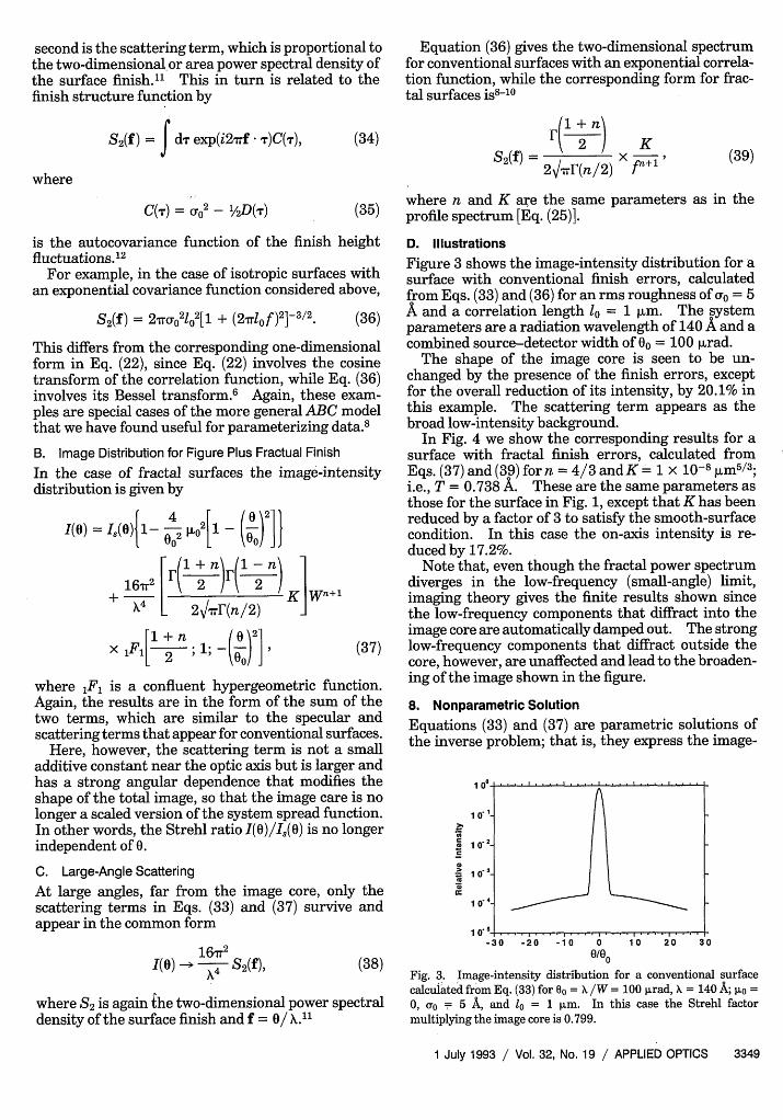
D. IllustrationsFigure 3 shows the image-intensity distribution for asurface with conventional finish errors, calculatedfrom Eqs. (33) and (36) for an rms roughness of u0 = 5A and a correlation length = 1 im. The systemparameters are a radiation wavelength of 140 A and acombined source-detector width of 00 = 100 grad.

The shape of the image core is seen to be un-changed by the presence of the finish errors, exceptfor the overall reduction of its intensity, by 20.1% inthis example. The scattering term appears as thebroad low-intensity background.

In Fig. 4 we show the corresponding results for asurface with fractal finish errors, calculated fromEqs. (37) and (39) for n = 4/3 and K = 1 X 10-8 gm 5/3;i.e., T = 0.738 A. These are the same parameters asthose for the surface in Fig. 1, except that K has beenreduced by a factor of 3 to satisfy the smooth-surfacecondition. In this case the on-axis intensity is re-duced by 17.2%.

Note that, even though the fractal power spectrumdiverges in the low-frequency (small-angle) limit,imaging theory gives the finite results shown sincethe low-frequency components that diffract into theimage core are automatically damped out. The stronglow-frequency components that diffract outside thecore, however, are unaffected and lead to the broaden-ing of the image shown in the figure.

8. Nonparametric SolutionEquations (33) and (37) are parametric solutions ofthe inverse problem; that is, they express the image-

1 T* 1

i 05 .,....,....,....,...,,..........-10. -2

1 0-

1 0

-30 -0 -0 0 1 0 36/00

Fig. 3. Image-intensity distribution for a conventional surfacecalculated from Eq. (33) for 00 = X /W = 100 prad, X = 140 A; po =0, oro = 5 A, and lo = 1 pm. In this case the Strehl factormultiplying the image core is 0.799.


10 0

amC

a

C}

1 0o '-

1 0'3-

1 0.1

I0 -30 -20 -10 0 10

0/00

03

20 30

Fig. 4. Image-intensity distribution for a fractal surface calcu-lated from Eq. (37) for the same system and figure parameters as inFig. 3, but n = 4/3 and K = 1 x 10-8 m5/3. In this case theon-axis Strehl factor is 0.828.

intensity distribution in terms of figure and finishparameters of the surface errors that can be mea-sured in the laboratory. They have the advantage ofgiving the entire image-intensity distribution but thedisadvantage of being model specific.

In this section we use the smooth-surface approxi-mation to develop nonparametric or model-indepen-dent connections between image properties and theprofile statistics. We do this by expanding the imageintensity in a power series in the angle observationangle 0 and expressing the results in terms of theprofile power spectrum by using Eq. (18). The firstterm in this expansion determines the on-axis Strehlfactor, and the next nonvanishing term, which isquadratic in 0, gives a measure of the image broaden-ing.

A. Effects on the On-Axis Image IntensityThe on-axis Strehl ratio is easily seen to be

I(O) = 1 - ) J df.'S,(f.')Ko(fx'), (40)

where the kernel in the integral over the errorspectrum is

Ko(f ) = 1 - 1F1[1; /2; -(Wfx )23.

q

Fig.5. Function K0 given by Eq. (41), where q = Wf, = 0/0o.

In the case of fractal surfaces the spectrum di-verges at low frequencies and the vanishing of thekernel at that point plays an essential role. Even so,the spectral integral can still be viewed as a mean-square roughness value, but one that is no longer anintrinsic property of the surface since it depends onthe system coherence length W.

The surface and system effects can be separated,however, and Eq. (40) can be written in terms ofintrinsic finish parameters by expressing Ko in termsof powers of (Wf') 2 and examining individual terms.For example, if we approximate it as

Ko(f.') 2 (Wfi )0 < f' 1,/V2Wotherwise (

we obtain the following neat result for the reductionof the on-axis intensity:

I(O) 1- (go 2 + uw2) - (4q) 2 (43)

where o is the rms figure gradient, which is relatedto its profile spectrum according to Eq. (20), and

=/2W

11 2

(41)

This is an important factor since it determines howthe different frequency components in the surfaceprofile f' affect the on-axis intensity.

The form of this kernel is shown in Fig. 5. Thefact that it vanishes at low frequencies means thatthe effects of long-wavelength components of thefigure and finish errors are attenuated, while thosewith wavelengths longer than the coherence length Wenter with full strength.

Equation (40) is valid for any form of the surfacespectrum. In the case of conventional surfaces themajor part of the spectral integral comes from highfrequencies where K = 1, the integral becomes themean-square surface roughness ro

2, and we obtain

the smooth-surface form of the conventional Strehlfactor appearing in Eq. (32).

(44)

crw 2

= Io (45)df'S21( fWt)/12W

are the band-width-limited values of the rms gradientand height of the finish errors.13 Note that thesequantities are finite for fractal surfaces, althoughtheir intrinsic values, determined by letting the limitsgo from zero to infinity, are undefined (infinite).

This approximate expression for the on-axis Strehlratio has simple and interesting dependencies onsystem parameters. The factor of 1/0o2 multiplyingthe surface-gradient terms comes from the curvatureof the system spread function on the optic axis and isindependent of in the case of system-limited optics,which means that these terms affect the image accord-ing to the rules of geometrical optics. The coefficientof the surface-roughness term, on the other hand,depends on the radiation wavelength but is indepen-


. . . .rB

df.'Si(f.')(27rf. 1)2,

dent of the system spread function, which accountsfor its historical precedence in the literature.

In other words, Eqs. (43)-(45) show that in thesmooth-surface limit, spatial wavelengths of the pro-file errors that diffract within the exp(- 1/2) = 0.607intensity point of the system spread function affectthe on-axis intensity according to the rules of geomet-rical optics, while those that diffract outside thatpoint deplete the core intensity without changing itsshape.

B. Effects on the Image WidthThe quadratic term in the expansion of the imageintensity about the optic axis determines the effects ofthe surface errors on the image width. There are anumber of ways to define image widths, the mostobvious being the rms width. This measure, how-ever, diverges when the image involves scatteringfrom objects with infinite rms slopes, such as unapo-dized apertures, surfaces with exponential correla-tion functions, and fractal surfaces. In such casesthe simplest practical measure is the parabolic width,that is, the half-width of the base of a parabola fittedto the apex of the image intensity:

. [ ~1 d 2 4(6)11-1/2-- -~~ I . (46)width I() A - 2 d02 11(0) ]1

The parabolic and rms widths of a two-dimensionalGaussian are the same, namely, 00.

The effect of errors on the parabolic image width isgiven by

width (0) 1 +4r2 'widthIJ(o) 1 X J - 2 (xx f.),

where the kernel

K 2(f') = 2(Wf ')2 F/[2; 3/2; (Wfx )'1

(47)

(48)

determines how the different frequency componentsin the surface profile affect the image width, just as Kodiscussed above determines their effects on the Strehlratio.

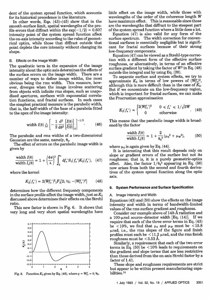
This new factor is shown in Fig. 6. It shows thatvery long and very short spatial wavelengths have

0.7- .... . . .... ....

0.6-

0.5-

0.4-

- 0.3-

0.2-

0 1 2 3 4 5q

Fig. 6. Function K2 given by Eq. (48), where q = WfX = O/Oo.

little effect on the image width, while those withwavelengths of the order of the coherence length Whave maximum effect. This is reasonable since thoseare the wavelengths that diffract to the steepest partof the system spread function where a little does a lot.

Equation (47) is also valid for any form of thesurface spectrum. The width correction for conven-tional surfaces is essentially negligible but is signifi-cant for fractal surfaces because of their stronglow-frequency components.

Equation (47) can be viewed as a Strehl-type correc-tion with a different form of the effective surfaceroughness, or alternatively, in terms of an effectivesurface gradient by taking the factor of W2 in Eq. (48)outside the integral and by using Eq. (20).

To separate surface and system effects, we try toapproximate K2 in terms of low powers of (Wf) 2,although this is more difficult than in the case of K 0.But if we concentrate on the low-frequency region,which is important for fractal surfaces, we can makethe Procrustian approximation

K 2( f.') {2(WTi) 20 < f' • 1/42W

otherwise

This means that the parabolic image width is broad-ened by the factor

width I(0)width IS(0)

1 + 2 (go 2 + gW2), (50)

where g.o is again given by Eq. (44).It is interesting that this result depends only on

slope or gradient errors of the surface but not itsroughness; that is, it is a purely geometric-opticseffect. Also, the factor 1/002 appearing in Eq. (50)now arises from both the second and fourth deriva-tives of the system spread function along the opticaxis.

9. System Performance and Surface Specification

A. Image Intensity and WidthEquations (43) and (50) show the effects on the imageintensity and width in terms of bandwidth-limitedvalues of the rms surface gradient and roughness.

Consider our example above of 140-A radiation anda 100-grad source-detector width [Eq. (14)]. If werequire that each of the three error terms in Eq. (43)be < 10%, we find that go and gw must be < 15.8grad, i.e., the rms slopes of the figure and finishprofiles must each be < 11.2 grad, and the rms finishroughness must be < 3.53 A.

Similarly, a requirement that each of the two errorterms in Eq. (50) be < 10% leads to requirements onthe gradient and slope terms that are less restrictivethan those derived from the on-axis Strehl factor by afactor of 1.41.

These slope and roughness requirements are strictbut appear to be within present manufacturing capa-bilities.14


B. Intensity of the Image TailEquation (38) shows that in the smooth-surface limita requirement on the intensity well away from theimage core translates to a requirement on the two-dimensional finish spectrum. This in turn is relatedto specific finish parameters through the form of thefinish spectrum involved; Eqs. (22) and (36) show anexample for conventional surfaces, and Eqs. (25) and(39) show general results for fractal surfaces.

C. Image-Frequency DistributionThe performance requirements considered above aregiven in terms of the image-intensity distribution inthe focal plane. Perhaps the simplest requirementson the image are stated in terms of its spatial-frequency content in that plane, which is nothingmore than the total OTF expressed in terms of thatnew frequency g:

OTF(g) = OTF8 (g) x exp[- - (- )D(g)], (51)

where g = f/XF. One specification might be thatthe total OTF must be greater than, say, 0.8 at aparticular frequency.

D. Hopkins Ratio

A more general condition is to require that theHopkins ratio,

H(g) = OTF8(g) (52)

be greater than some function or value.' 5 Since Eqs.(51) and (52) involve the exponential dependence onthe structure function, they are not limited to thesmooth-surface approximation.

In general, performance requirements on the im-age intensity lead to conditions on the spectrum ofthe errors, while those on the OTF place conditionson its structure function.

10. Physical InterpretationBoth the parametric and nonparametric expressionsfor the image-intensity distribution are finite forfractal surface, even though the fractal spectrumdiverges at long spatial wavelengths, which suggeststhat the scattering should diverge at small angles.

Physically, the divergence disappears since thefinite size of the imaging optic makes the systeminsensitive to surface wavelengths longer than itsdiameter Do, and the wavelengths between Do and Ware attenuated by convolution with the nonvanishingsource and detector sizes.

There is an interesting corollary to this. Mostcalculations of surface scattering are based on themodel of an infinite surface coherently illuminated byan incident plane wave, i.e., W = - in our notation.'1' 9

In that case the only way to avoid small-angle diver-gences is to require that the error spectrum be wellbehaved at low frequencies, which means that the

surface roughness itself must involve a finite-lengthscale or correlation length. In other words, pureplane-wave scattering calculations require conven-tional surfaces.' 2

In the present paper we point out that in real-worldsituations the finish of high-performance surfaces arefrequently fractal and that in those cases the finiteouter length scale required for finite scattering isintroduced by system parameters, either the finitesize of the optic for diffraction-limited optics or thesystem coherence length W for system-limited optics.

Finally, it is interesting to note that the fractalfinish may be expected since the essence of a well-finished surface is that it is featureless, or in mathe-matical terms, that it is self-affine or fractal.

1 1. SummaryWe have described a simple diffraction calculation forpredicting the image of an imperfect mirror in termsof system and surface properties. When the imagingis system limited, as is frequently the case for x-rayoptics, the diffraction integral depends on the effec-tive coherence length of the radiation on the mirrorsurface, which is smaller than its aperture, as well asthe error properties of the surface.

Roughly speaking, those spatial-wavelength compo-nents of the mirror-shape errors that are longer thanthe coherence length behave according to the rules ofgeometrical optics, while those with shorter spatialwavelengths behave according to diffraction optics.

In the smooth-surface limit, parametric and non-parametric expressions are given that can be used tospecify surface properties in terms of performancerequirements. The parametric expressions are func-tions of parameters of specific finish models, while thenonparametric forms are expressed in terms of theprofile-power spectral density of the surfaces whichcan be measured directly in the laboratory.

Results are illustrated for two models: figure plusconventional finish, where the finish correlationlength is comparable with or smaller than the coher-ence length, and figure plus fractal finish, where thecorrelation length is larger than the coherence lengthor effectively infinite. The results are well behavedeven in the limiting case of pure fractal surfaces,where the correlation length becomes infinite and thepower spectral density diverges at low frequencies.

References and Notes1. E. L. Church and P. Z. Takacs, "Prediction of mirror perfor-

mance from laboratory measurements," inX-Ray/EUVOpticsfor Astronomy and Microscopy, R. B. Hoover, ed., Proc. Soc.Photo-Opt. Instrum. Eng. 1160, 323-336 (1989). This refer-ence discusses the system-limited behavior of glancing-incidence mirrors in terms of their one-dimensional or profilepower spectra.

2. E. L. Church and P. Z. Takacs, "Specification of the surfacefigure and finish of optical elements in terms of systemperformance," in Specification and Measurement of OpticalSystems, L. R. Baker, ed., Proc. Soc. Photo-Opt. Instrum. Eng.1781, 118-130 (1992). This reference extends the researchin Ref. 1 to normal-incidence optics and expresses the resultsin terms of the two-dimensional or area power spectra.


3. E. L. Church and P. Z. Takacs, "Specifying the surface finishof x-ray mirrors," in Soft-X-Ray Projection Lithography, Vol.18 of OSA Proceedings Series (Optical Society of America,Washington, D.C., 1993). This reference extends the re-search in Ref. 2 to diffraction-limited optics.

4. The Gaussian forms of Eq. (15), (31), (32), and (51) follow fromthe assumption that the error fluctuations are members of aGaussian random process with a Gaussian height distribution.In the more general case of a kth-order gamma distribution,Eq. (15) is replaced by OTF(r) = [1 + (4r/ X)2D('r)/2k]- k Inthe smooth-surface limit, however, results are independent ofthe form of the height distribution.

5. The -statistical stability of the results is ensured by thesmallness of the parameter (W/Do)2.

6. Si(f.) and S2(f) are the cosine and zeroth-order Hankeltransforms of a common correlation function and form, then,an Abel-transform pair. That is, S, is the two-to-one-dimensional stereological projection or half-integral of S2.See also Ref. 9.

7. E. L. Church and P. Z. Takacs, "Instrumental effects insurface finish measurements," in Surface Measurement andCharacterization, J. M. Bennett, ed., Proc. Soc. Photo-Opt.Instrum. Eng. 1009, 46-55 (1988).

8. E. L. Church and P. Z. Takacs, "The optimal estimation offinish parameters," in Optical Scatter: Applications, Measure-ment, and Theory, J. C. Stover, ed., Proc. Soc. Photo-Opt.Instrum. Eng. 1530, 71-86 (1991).

9. E. L. Church, H. A. Jenkinson, and J. M. Zavada, "Relation-ship between surface scattering and microtopographic fea-tures," Opt. Eng. 18, 125-136 (1979).

10. E. L. Church, "Fractal surface finish," Appl. Opt. 27, 1518-1526 (1988). The coefficient 45 in Eq. (A5) of this referenceshould read 74.

11. The bars over the two-dimensional power spectra in Eqs. (33)and (38) denote their convolution with the system spreadfunction, Eq. (13). This has a negligible effect for polishedsurfaces but would, for example, determine the nonvanishingwidths of the spectral lines caused by periodic tool marks inmachined surfaces.

12. Statistical scattering theory depends on the structure functionof the surface-height fluctuations and not their autocovariancefunction. The structure function exists when the fluctua-tions have statistically stationary first differences, while theautocovariance function exists only in the more restrictivecondition that the magnitudes themselves are also stationary.Fractal surfaces have stationary differences but nonstationarymagnitudes, while conventional surfaces have stationary differ-ences and magnitudes. A telltale difference is whether thesurface in question has a finite intrinsic rms roughness.Conventional surfaces do; fractal surfaces do not.

13. More precisely, the limits 0 and o in Eqs. (44) and (45) are 2/Doand 2/X.

14. Melles Griot Industrie (France) advertises x-ray mirrors withrms slopes of < 5 prad and rms roughnesses of < 5 A. An rmsslope of 5 prad corresponds to an rms gradient of 7 prad.

15. H. H. Hopkins, "The aberration permissible in optical systems,"Proc. Phys. Soc. London Sec. B 52, 449-470 (1957).

16. P. Beckmann and A. Spizzichino, The Scattering of Electroma-gentci Waves from Rough Surfaces (Pergamon, New York,1963).

17. S. K. Sinha, E. B. Sirota, S. Garoff, and H. B. Stanley, "X-rayand neutron scattering from rough surfaces," Phys. Rev. B 38,2297-2311 (1988).

18. D. G. Stearns, "X-ray scattering from nonideal multilayerstructures," J. Appl. Phys. 65, 491-506 (1989).

19. D. G. Stearns, "X-ray scattering from interfacial roughness inmultilayer structures," J. Appl. Phys. 71, 4286-4298 (1992).


Documents

Specification of surface figure and finish in terms of system performance