Embed Size (px)
Citation preview
Specifying Concurrent Systems with
TLA+
Leslie Lamport
24 Dec 1999
c©1999 by Leslie Lamport
Preliminary Draft
Be sure to read the description of this document onpage 3 of the Introduction.

Contents
Introduction . . . . . . . . . . . . . . . . . . . . . . . . . . . . . . . . . 1
I Getting Started 5
1 A Little Simple Math 91.1 Propositional Logic . . . . . . . . . . . . . . . . . . . . . . . . . . 91.2 Sets . . . . . . . . . . . . . . . . . . . . . . . . . . . . . . . . . . 111.3 Predicate Logic . . . . . . . . . . . . . . . . . . . . . . . . . . . . 12
2 Specifying a Simple Clock 152.1 Behaviors . . . . . . . . . . . . . . . . . . . . . . . . . . . . . . . 152.2 An Hour Clock . . . . . . . . . . . . . . . . . . . . . . . . . . . . 152.3 A Closer Look at the Hour-Clock Specification . . . . . . . . . . 182.4 The Hour-Clock Specification in TLA+ . . . . . . . . . . . . . . . 192.5 Another Way to Specify the Hour Clock . . . . . . . . . . . . . . 21
3 An Asynchronous Interface 233.1 The First Specification . . . . . . . . . . . . . . . . . . . . . . . . 243.2 Another Specification . . . . . . . . . . . . . . . . . . . . . . . . 283.3 Types: A Reminder . . . . . . . . . . . . . . . . . . . . . . . . . 303.4 Definitions . . . . . . . . . . . . . . . . . . . . . . . . . . . . . . . 313.5 Comments . . . . . . . . . . . . . . . . . . . . . . . . . . . . . . . 32
4 A FIFO 354.1 The Inner Specification . . . . . . . . . . . . . . . . . . . . . . . 354.2 Instantiation Examined . . . . . . . . . . . . . . . . . . . . . . . 37
4.2.1 Instantiation is Substitution . . . . . . . . . . . . . . . . . 374.2.2 Parametrized Instantiation . . . . . . . . . . . . . . . . . 394.2.3 Implicit Substitutions . . . . . . . . . . . . . . . . . . . . 394.2.4 Instantiation Without Renaming . . . . . . . . . . . . . . 40
4.3 Hiding the Queue . . . . . . . . . . . . . . . . . . . . . . . . . . . 414.4 A Bounded FIFO . . . . . . . . . . . . . . . . . . . . . . . . . . . 41
3
4 CONTENTS
4.5 What We’re Specifying . . . . . . . . . . . . . . . . . . . . . . . . 43
5 A Caching Memory 455.1 The Memory Interface . . . . . . . . . . . . . . . . . . . . . . . . 455.2 Functions . . . . . . . . . . . . . . . . . . . . . . . . . . . . . . . 485.3 A Linearizable Memory Specification . . . . . . . . . . . . . . . . 505.4 Tuples as Functions . . . . . . . . . . . . . . . . . . . . . . . . . 515.5 Recursive Function Definitions . . . . . . . . . . . . . . . . . . . 535.6 A Write-Through Cache . . . . . . . . . . . . . . . . . . . . . . . 545.7 Invariance . . . . . . . . . . . . . . . . . . . . . . . . . . . . . . . 605.8 Proving Implementation . . . . . . . . . . . . . . . . . . . . . . . 62
6 Some More Math 656.1 Sets . . . . . . . . . . . . . . . . . . . . . . . . . . . . . . . . . . 656.2 Silly Expressions . . . . . . . . . . . . . . . . . . . . . . . . . . . 676.3 Recursive Function Definitions Revisited . . . . . . . . . . . . . . 676.4 Functions versus Operators . . . . . . . . . . . . . . . . . . . . . 696.5 Using Functions . . . . . . . . . . . . . . . . . . . . . . . . . . . . 716.6 Choose . . . . . . . . . . . . . . . . . . . . . . . . . . . . . . . . . 72
7 Writing a Specification—Some Advice 757.1 Why to Specify . . . . . . . . . . . . . . . . . . . . . . . . . . . . 757.2 What to Specify . . . . . . . . . . . . . . . . . . . . . . . . . . . 767.3 The Grain of Atomicity . . . . . . . . . . . . . . . . . . . . . . . 767.4 The Data Structures . . . . . . . . . . . . . . . . . . . . . . . . . 787.5 Writing the Specification . . . . . . . . . . . . . . . . . . . . . . . 797.6 Some Further Hints . . . . . . . . . . . . . . . . . . . . . . . . . . 797.7 When and How to Specify . . . . . . . . . . . . . . . . . . . . . . 82
II More Advanced Topics 85
8 Liveness and Fairness 878.1 Temporal Formulas . . . . . . . . . . . . . . . . . . . . . . . . . . 878.2 Weak Fairness . . . . . . . . . . . . . . . . . . . . . . . . . . . . . 918.3 Liveness for the Memory Specification . . . . . . . . . . . . . . . 948.4 Strong Fairness . . . . . . . . . . . . . . . . . . . . . . . . . . . . 958.5 Liveness for the Write-Through Cache . . . . . . . . . . . . . . . 978.6 Quantification . . . . . . . . . . . . . . . . . . . . . . . . . . . . . 988.7 Temporal Logic Examined . . . . . . . . . . . . . . . . . . . . . . 100
8.7.1 A Review . . . . . . . . . . . . . . . . . . . . . . . . . . . 1008.7.2 Machine Closure . . . . . . . . . . . . . . . . . . . . . . . 1008.7.3 Machine Closure and Possibility . . . . . . . . . . . . . . 1028.7.4 The Unimportance of Liveness . . . . . . . . . . . . . . . 103
CONTENTS 5
8.7.5 Temporal Logic Considered Confusing . . . . . . . . . . . 103
9 Real Time 1059.1 The Hour Clock Revisited . . . . . . . . . . . . . . . . . . . . . . 1059.2 Real-Time Specifications in General . . . . . . . . . . . . . . . . 1089.3 The Real-Time Write-Through Cache . . . . . . . . . . . . . . . 1129.4 Zeno Specifications . . . . . . . . . . . . . . . . . . . . . . . . . . 1179.5 Hybrid System Specifications . . . . . . . . . . . . . . . . . . . . 1199.6 Remarks on Real Time . . . . . . . . . . . . . . . . . . . . . . . . 121
10 Composing Specifications 12310.1 Composing Two Specifications . . . . . . . . . . . . . . . . . . . 12410.2 Composing Many Specifications . . . . . . . . . . . . . . . . . . . 12610.3 The FIFO . . . . . . . . . . . . . . . . . . . . . . . . . . . . . . . 12910.4 Composition with Shared State . . . . . . . . . . . . . . . . . . . 132
10.4.1 Explicit State Changes . . . . . . . . . . . . . . . . . . . . 13210.4.2 Composition with Joint Actions . . . . . . . . . . . . . . . 135
10.5 A Brief Review . . . . . . . . . . . . . . . . . . . . . . . . . . . . 13910.5.1 A Taxonomy of Composition . . . . . . . . . . . . . . . . 13910.5.2 Interleaving Reconsidered . . . . . . . . . . . . . . . . . . 13910.5.3 Joint Actions Reconsidered . . . . . . . . . . . . . . . . . 140
10.6 Liveness and Hiding . . . . . . . . . . . . . . . . . . . . . . . . . 14110.6.1 Liveness and Machine Closure . . . . . . . . . . . . . . . . 14110.6.2 Hiding . . . . . . . . . . . . . . . . . . . . . . . . . . . . . 142
10.7 Open-System Specifications . . . . . . . . . . . . . . . . . . . . . 14410.8 Interface Refinement . . . . . . . . . . . . . . . . . . . . . . . . . 146
10.8.1 A Binary Hour Clock . . . . . . . . . . . . . . . . . . . . 14610.8.2 Refining a Channel . . . . . . . . . . . . . . . . . . . . . . 14810.8.3 Interface Refinement in General . . . . . . . . . . . . . . . 15110.8.4 Open-System Specifications . . . . . . . . . . . . . . . . . 153
10.9 Should You Compose? . . . . . . . . . . . . . . . . . . . . . . . . 155
11 Advanced Examples 15711.1 Specifying Data Structures . . . . . . . . . . . . . . . . . . . . . 158
11.1.1 Local Definitions . . . . . . . . . . . . . . . . . . . . . . . 15811.1.2 Graphs . . . . . . . . . . . . . . . . . . . . . . . . . . . . 15911.1.3 Solving Differential Equations . . . . . . . . . . . . . . . . 16311.1.4 The Riemann Integral . . . . . . . . . . . . . . . . . . . . 165
11.2 Other Memory Specifications . . . . . . . . . . . . . . . . . . . . 16511.2.1 The Interface . . . . . . . . . . . . . . . . . . . . . . . . . 16811.2.2 The Correctness Condition . . . . . . . . . . . . . . . . . 16811.2.3 A Serial Memory . . . . . . . . . . . . . . . . . . . . . . . 17111.2.4 A Sequentially Consistent Memory . . . . . . . . . . . . . 17811.2.5 The Memory Specifications Considered . . . . . . . . . . . 183
6 CONTENTS
III The Tools 187
12 The Java Front End 18912.1 Finding an Error . . . . . . . . . . . . . . . . . . . . . . . . . . . 189
13 The TLC Model Checker 19113.1 Introduction to TLC . . . . . . . . . . . . . . . . . . . . . . . . . 19113.2 How TLC Works . . . . . . . . . . . . . . . . . . . . . . . . . . . 198
13.2.1 TLC Values . . . . . . . . . . . . . . . . . . . . . . . . . . 19813.2.2 How TLC Evaluates Expressions . . . . . . . . . . . . . . 19913.2.3 Assignment and Replacement . . . . . . . . . . . . . . . . 20113.2.4 Overriding Modules . . . . . . . . . . . . . . . . . . . . . 20313.2.5 How TLC Computes States . . . . . . . . . . . . . . . . . 20313.2.6 When TLC Computes What . . . . . . . . . . . . . . . . 20413.2.7 Random Simulation . . . . . . . . . . . . . . . . . . . . . 205
13.3 How to Use TLC . . . . . . . . . . . . . . . . . . . . . . . . . . . 20613.3.1 Running TLC . . . . . . . . . . . . . . . . . . . . . . . . . 20613.3.2 Debugging a Specification . . . . . . . . . . . . . . . . . . 20713.3.3 The TLC Module . . . . . . . . . . . . . . . . . . . . . . 21213.3.4 Checking Action Invariance . . . . . . . . . . . . . . . . . 21413.3.5 Checking Implementation . . . . . . . . . . . . . . . . . . 21713.3.6 Some Hints . . . . . . . . . . . . . . . . . . . . . . . . . . 218
13.4 What TLC Doesn’t Do . . . . . . . . . . . . . . . . . . . . . . . . 22113.5 Future Plans . . . . . . . . . . . . . . . . . . . . . . . . . . . . . 22313.6 The Fine Print: What TLC Really Does . . . . . . . . . . . . . . 224
13.6.1 TLC Values . . . . . . . . . . . . . . . . . . . . . . . . . . 22413.6.2 Overridden Values . . . . . . . . . . . . . . . . . . . . . . 22513.6.3 Expression Evaluation . . . . . . . . . . . . . . . . . . . . 22513.6.4 Fingerprinting . . . . . . . . . . . . . . . . . . . . . . . . 234
IV The TLA+ Language 235
14 The Syntax of TLA+ 24514.1 The Simple Grammar . . . . . . . . . . . . . . . . . . . . . . . . 246
14.1.1 BNF Grammars . . . . . . . . . . . . . . . . . . . . . . . 24614.1.2 The BNF Grammar of TLA+ . . . . . . . . . . . . . . . . 250
14.2 The Complete Grammar . . . . . . . . . . . . . . . . . . . . . . . 25814.2.1 Precedence and Associativity . . . . . . . . . . . . . . . . 25814.2.2 Alignment . . . . . . . . . . . . . . . . . . . . . . . . . . . 26114.2.3 Comments . . . . . . . . . . . . . . . . . . . . . . . . . . . 26214.2.4 Temporal Formulas . . . . . . . . . . . . . . . . . . . . . . 26314.2.5 Two Anomalies . . . . . . . . . . . . . . . . . . . . . . . . 264
14.3 What You Type . . . . . . . . . . . . . . . . . . . . . . . . . . . 264

CONTENTS 7
15 The Operators of TLA+ 26515.1 Constant Operators . . . . . . . . . . . . . . . . . . . . . . . . . 265
15.1.1 Boolean Operators . . . . . . . . . . . . . . . . . . . . . . 26715.1.2 The Choose Operator . . . . . . . . . . . . . . . . . . . . 26815.1.3 The Three Interpretations of Boolean Operators . . . . . 27015.1.4 Conditional Constructs . . . . . . . . . . . . . . . . . . . 27215.1.5 LET . . . . . . . . . . . . . . . . . . . . . . . . . . . . . . 27215.1.6 The Operators of Set Theory . . . . . . . . . . . . . . . . 27315.1.7 Functions . . . . . . . . . . . . . . . . . . . . . . . . . . . 27515.1.8 Records . . . . . . . . . . . . . . . . . . . . . . . . . . . . 27915.1.9 Tuples . . . . . . . . . . . . . . . . . . . . . . . . . . . . . 28015.1.10Strings . . . . . . . . . . . . . . . . . . . . . . . . . . . . . 28115.1.11Numbers . . . . . . . . . . . . . . . . . . . . . . . . . . . 282
15.2 Nonconstant Operators . . . . . . . . . . . . . . . . . . . . . . . 28315.2.1 The Meaning of a Basic Constant Expression . . . . . . . 28315.2.2 The Meaning of a State Function . . . . . . . . . . . . . . 28415.2.3 Action Operators . . . . . . . . . . . . . . . . . . . . . . . 28615.2.4 Temporal Operators . . . . . . . . . . . . . . . . . . . . . 288
16 The Meaning of a Module 29116.1 Operators and Expressions . . . . . . . . . . . . . . . . . . . . . 291
16.1.1 The Order and Arity of an Operator . . . . . . . . . . . . 29216.1.2 λ Expressions . . . . . . . . . . . . . . . . . . . . . . . . . 29316.1.3 Simplifying Operator Application . . . . . . . . . . . . . . 29416.1.4 Expressions . . . . . . . . . . . . . . . . . . . . . . . . . . 295
16.2 Levels . . . . . . . . . . . . . . . . . . . . . . . . . . . . . . . . . 29516.3 Contexts . . . . . . . . . . . . . . . . . . . . . . . . . . . . . . . . 29816.4 The Meaning of a λ Expression . . . . . . . . . . . . . . . . . . . 29916.5 The Meaning of a Module . . . . . . . . . . . . . . . . . . . . . . 301
16.5.1 Extends . . . . . . . . . . . . . . . . . . . . . . . . . . . . 30216.5.2 Declarations . . . . . . . . . . . . . . . . . . . . . . . . . . 30216.5.3 Operator Definitions . . . . . . . . . . . . . . . . . . . . . 30316.5.4 Function Definitions . . . . . . . . . . . . . . . . . . . . . 30316.5.5 Instantiation . . . . . . . . . . . . . . . . . . . . . . . . . 30416.5.6 Theorems and Assumptions . . . . . . . . . . . . . . . . . 30516.5.7 Submodules . . . . . . . . . . . . . . . . . . . . . . . . . . 305
16.6 Correctness of a Module . . . . . . . . . . . . . . . . . . . . . . . 30616.7 Finding Modules . . . . . . . . . . . . . . . . . . . . . . . . . . . 30616.8 The Semantics of Instantiation . . . . . . . . . . . . . . . . . . . 307
8 CONTENTS
17 The Standard Modules 31317.1 Module Sequences . . . . . . . . . . . . . . . . . . . . . . . . . . 31317.2 Module FiniteSets . . . . . . . . . . . . . . . . . . . . . . . . . . 31417.3 Module Bags . . . . . . . . . . . . . . . . . . . . . . . . . . . . . 31417.4 The Numbers Modules . . . . . . . . . . . . . . . . . . . . . . . . 318
V Appendix 323
A The ASCII Specifications 325A.1 The Asynchronous Interface . . . . . . . . . . . . . . . . . . . . . 325A.2 A FIFO . . . . . . . . . . . . . . . . . . . . . . . . . . . . . . . . 326A.3 A Caching Memory . . . . . . . . . . . . . . . . . . . . . . . . . . 327A.4 The Alternating Bit Protocol . . . . . . . . . . . . . . . . . . . . 332
References 335
List of Figures
2.1 The hour clock specification—typeset and ASCII versions. . . . . 20
3.1 The First Specification of an Asynchronous Interface . . . . . . . 273.2 Our second specification of an asynchronous interface. . . . . . . 303.3 The hour clock specification with comments. . . . . . . . . . . . 33
4.1 The specification of a FIFO, with the internal variable q visible. 384.2 Specification of a FIFO buffer of length N. . . . . . . . . . . . . . 43
5.1 The Specification of a Memory Interface . . . . . . . . . . . . . . 485.2 The internal memory specification (beginning). . . . . . . . . . . 525.3 The internal memory specification (end). . . . . . . . . . . . . . . 535.4 The memory specification. . . . . . . . . . . . . . . . . . . . . . . 535.5 The write-through cache specification (beginning). . . . . . . . . 565.6 The write-through cache specification (middle). . . . . . . . . . . 575.7 The write-through cache specification (end). . . . . . . . . . . . . 58
9.1 The real-time specification of an hour clock. . . . . . . . . . . . . 1099.2 The RealTime module for writing real-time specifications. . . . . 1129.3 A real-time version of the linearizable memory specification. . . . 1139.4 A real-time version of the write-through cache (beginning). . . . 1169.5 A real-time version of the write-through cache (end). . . . . . . . 117
10.1 A noninterleaving composite specification of the FIFO. . . . . . . 13110.2 A joint-action compositional specification of the linearizable mem-
ory. . . . . . . . . . . . . . . . . . . . . . . . . . . . . . . . . . . . 13810.3 A specification of a binary hour clock. . . . . . . . . . . . . . . . 14810.4 Refining a channel. . . . . . . . . . . . . . . . . . . . . . . . . . . 150
11.1 A module for specifying operators on graphs. . . . . . . . . . . . 16211.2 A module for specifying the solution to a differential equation. . 16611.3 A specification of the Riemann integral. . . . . . . . . . . . . . . 16711.4 A module for specifying a register interface to a memory. . . . . 169
9
10 LIST OF FIGURES
11.5 Module InnerSerial (beginning). . . . . . . . . . . . . . . . . . . 17911.6 Module InnerSerial (middle). . . . . . . . . . . . . . . . . . . . . 18011.7 Module InnerSerial (end). . . . . . . . . . . . . . . . . . . . . . . 18111.8 Module InnerSequential (beginning). . . . . . . . . . . . . . . . . 18411.9 Module InnerSequential (end). . . . . . . . . . . . . . . . . . . . 185
13.1 The Alternating Bit Protocol (beginning) . . . . . . . . . . . . . 19413.2 The Alternating Bit Protocol (end) . . . . . . . . . . . . . . . . . 19513.3 Module MCAlternatingBit. . . . . . . . . . . . . . . . . . . . . . 19613.4 A configuration file for module MCAlternatingBit. . . . . . . . . 19713.5 The standard module TLC . . . . . . . . . . . . . . . . . . . . . 21313.6 An invariant of the alternating bit protocol’s next-state action. . 21513.7 A higher-level specification of the alternating bit protocol. . . . . 21813.8 A module for checking the alternating bit protocol. . . . . . . . . 21913.9 The constant operators. . . . . . . . . . . . . . . . . . . . . . . . 23813.10Miscellaneous constructs. . . . . . . . . . . . . . . . . . . . . . . 23913.11Action operators. . . . . . . . . . . . . . . . . . . . . . . . . . . . 23913.12Temporal operators. . . . . . . . . . . . . . . . . . . . . . . . . . 23913.13User-definable operator symbols. . . . . . . . . . . . . . . . . . . 24013.14The precedence ranges of operators. . . . . . . . . . . . . . . . . 24113.15Operators defined in the standard modules. . . . . . . . . . . . . 24213.16The ascii representations of typeset symbols. . . . . . . . . . . . 243
14.1 The definition of the grammar GSE for the language SE. . . . . 25014.2 The module BNFGrammars . . . . . . . . . . . . . . . . . . . . . 251
17.1 The standard Sequences module. . . . . . . . . . . . . . . . . . . 31517.2 The standard FiniteSets module. . . . . . . . . . . . . . . . . . . 31517.3 The standard Bags module. . . . . . . . . . . . . . . . . . . . . . 31717.4 The Peano module. . . . . . . . . . . . . . . . . . . . . . . . . . . 31917.5 The ProtoReals module (beginning). . . . . . . . . . . . . . . . . 32017.6 The ProtoReals module (end). . . . . . . . . . . . . . . . . . . . . 32117.7 The standard Naturals module. . . . . . . . . . . . . . . . . . . . 32217.8 The standard Integers module. . . . . . . . . . . . . . . . . . . . 32217.9 The standard Reals module. . . . . . . . . . . . . . . . . . . . . . 322
Introduction
Writing is nature’s way of letting youknow how sloppy your thinking is.
Guindon
Writing a specification for a system helps us understand it. It’s a good idea tounderstand something before you build it, so it’s a good idea to specify a systembefore you implement it.
Mathematics is nature’s way of letting you know how sloppy your writing is.Specifications written in an imprecise language like English are usually imprecise.In engineering, imprecision is an invitation to error. Science and engineeringhave adopted mathematics as a language for writing precise descriptions.
Formal mathematics is nature’s way of letting you know how sloppy yourmathematics is. The mathematics written by most mathematicians and scien-tists is still imprecise. Most mathematics texts are precise in the small, butimprecise in the large. Each equation is a precise assertion, but you have toread the text to understand how the equations relate to one another, and whatthe theorems really mean. Logicians have developed ways of eliminating thewords and formalizing mathematics.
Most mathematicians and computer scientists think that writing mathemat-ics formally, without words, is tiresome. I’ve asked a number of computer scien-tists the following question: How long would a formal specification of the Rie-mann integral of elementary calculus be, assuming only arithmetic operationson real numbers. The answers I received ranged up to 50 pages. Section 11.1.4shows how to do it in about 20 lines. Once you learn how, it’s easy to expressordinary mathematics in a precise, completely formal language.
To specify systems with mathematics, we must decide what kind of mathe-matics to use. We can specify an ordinary sequential program by describing itsoutput as a function of its input. So, sequential programs can be specified interms of functions. Concurrent systems are usually described in terms of theirbehaviors—what they do in the course of an execution. In 1977, Amir Pnueliintroduced the use of temporal logic for describing such behaviors.
Temporal logic is appealing because, in principle, it allows a concurrent sys-tem to be described by a single formula. In practice, temporal logic proved to be
1
2 LIST OF FIGURES
cumbersome. Pnueli’s temporal logic was ideal for describing some properties ofsystems, but awkward for others. So, it was usually combined with some moretraditional way of describing systems.
In the late 1980’s, I discovered TLA, the Temporal Logic of Actions. TLAis a simple variant of Pnueli’s original logic that makes it practical to writea specification as a single formula. Most of a TLA specification consists ofordinary, nontemporal mathematics. Temporal logic plays a significant role onlyin describing those properties that it’s good at describing. TLA also provides anice way to formalize the style of reasoning about systems that has proved tobe most effective in practice—a style known as assertional reasoning. However,the topic of this document is specification, not proof, so I will have little to sayabout proofs.
TLA provides a mathematical foundation for describing concurrent systems.To write specifications, we need a complete language built atop that foundation.I initially thought that this language should be some sort of abstract program-ming language whose semantics would be based on TLA. I didn’t know whatkind of programming language constructs would be best, so I decided to startwriting specifications directly in TLA. I intended to introduce programmingconstructs as I needed them. To my surprise, I discovered that I didn’t needthem. What I needed was a robust language for writing mathematics.
Although mathematicians have developed the science of writing formulas,they haven’t turned that science into an engineering discipline. They have de-veloped notations for mathematics in the small, but not for mathematics in thelarge. The specification of a real system can be dozens or even hundreds of pageslong. Mathematicians know how to write 20-line formulas, not 20-page formulas.So, I had to introduce notations for writing long formulas. What I took fromprogramming languages were ideas for modularizing large specifications.
The language I came up with is called TLA+. I refined TLA+ in the courseof writing specifications of disparate systems. But it has changed little in thelast few years. I have found TLA+ to be quite good for specifying a wide classof systems—from program interfaces (APIs) to distributed systems. It can beused to write a precise, formal description of almost any sort of discrete system.It’s especially well suited to describing asynchronous systems—that is, systemswith components that do not operate in strict lock-step.
One advantage of a precise specification language is that it enables us tobuild tools that can help us write correct specifications. There are now at leasttwo such tools under development: a parser and a model checker, described inPart III. The parser can catch simple errors in any TLA+ specification. Themodel checker can catch many more errors, but it works on a restricted class ofspecifications—a class that seems to include most of the specifications of interestto industry today.
LIST OF FIGURES 3
The State of this Document
This document is a preliminary draft. Here is a brief description of the individualparts what and who should read them.
Part I
These chapters are complete and shouldn’t have too many errors. They are anintroduction and should be read by everyone interested in using TLA+. Theyexplain how to specify the class of properties known as safety properties. Theseproperties, which can be specified with almost no temporal logic, are all thatmost engineers need to know about.
Part II
Temporal logic comes to the fore in Chapter 8, where it is used to specify theadditional class of properties known as liveness properties. This chapter is inpretty good shape, but probably has more errors per page than the precedingchapters. The remaining chapters in this part are rough drafts and are full oferrors. Chapter 9 describes how to specify real-time properties, and Chapter 10describes how to write specifications as compositions. Chapter 11 describes somemore advanced examples.
Part III
This part describes the parser and the TLC model checker. If you are readingthis because you want to use TLA+, then you’ll probably want to use these toolsand should read these chapters. They are preliminary and have lots of errors.Before trying to use TLC be sure to read Section 13.4 on page 221; it describeslimitations of the current version of the program.
Part IV
This part is a reference manual for the language. It has not been read carefullyand is undoubtedly full of errors. Part I should give you a good enough work-ing knowledge of the language for most of your needs. Part IV describes thefine points of the syntax and semantics; it also contains the standard modules.Chapter 14 gives the syntax of TLA+ and includes a BNF grammar (writtenin TLA+). Chapter 15 describes the precise meanings and the general forms ofall the built-in operators of TLA+. It should answer any questions you mighthave about exactly a TLA+ operator means. Chapter 16 describes the precisemeaning of all the higher-level TLA+ constructs, such as definitions and moduleinclusion. Chapters 15 and 16 together specify the semantics of the language.
4 LIST OF FIGURES
Chapter 17 describes the standard modules—except for module RealTime, de-scribed in Chapter 9, and module TLC , described in Chapter 13. You mightwant to look at this chapter if you’re curious about how standard elementarymathematics can be formalized in TLA+.
You will seldom have occasion to read any of Part IV. However, it doeshave something you may want to refer to often: a mini-manual that compactlypresents lots of useful information. Pages 238–243 list all TLA+ operators, alluser-definable symbols, the precedence of all operators, all operators defined inthe standard modules, and the ascii representation of symbols like ⊗.
The Appendix
The specifications that appear in the book are typeset for easy reading by hu-mans. To be read by a tool, a specification must be written in ascii. Theappendix includes the ascii versions of all the specifications in Part I, as wellas the specifications from Chapter 13. Comparing the ascii and the typesetversion can teach you how to write TLA+ specifications in ascii.

Part I
Getting Started
5

7
A system specification consists of a lot of ordinary mathematics glued to-gether with a little bit of temporal logic. So, most of the work in writing a pre-cise specification consists of expressing ordinary mathematics precisely. That’swhy most of the details of TLA+ are concerned with expressing ordinary math-ematics.
Unfortunately, the computer science departments in many universities ap-parently believe that fluency in C++ is more important than a sound educationin elementary mathematics. So, some readers may be unfamiliar with the math-ematics needed to write specifications. Fortunately, this mathematics is quitesimple. If overexposure to C++ hasn’t destroyed your ability to think logically,you should have no trouble filling any gaps in your mathematics education. Youprobably learned arithmetic before being exposed to C++, so I will assume youknow about numbers and arithmetic operations on them.1 I will try to explainall other mathematical concepts that you need, starting in Chapter 1 with areview of some elementary math. I hope most readers will find this reviewcompletely unnecessary.
After the brief review of simple mathematics in the next section, Chapters2 through 5 describe TLA+ with a sequence of examples. Chapter 6 explainssome more about the math used in writing specifications, and Chapter 7 reviewseverything and provides some advice. By the time you finish Chapter 7, youshould be able to handle most of the specification problems that you are likelyto encounter in ordinary engineering practice.
1Some readers may need reminding that numbers are not strings of bits, and 233 ∗ 233
equals 266, not overflow error.

8
Chapter 1
A Little Simple Math
1.1 Propositional Logic
Elementary algebra is the mathematics of real numbers and the operators +,−, ∗ (multiplication), and / (division). Propositional logic is the mathematicsof the two Boolean values true and false and the five operators whose names(and common pronunciations) are:
∧ conjunction (and)∨ disjunction (or)≡ equivalence (is equivalent to)
¬ negation (not)⇒ implication (implies)
To learn how to compute with numbers, you had to memorize addition andmultiplication tables and algorithms for calculating with multidigit numbers.Propositional logic is much simpler, since there are only two values, true andfalse. To learn how to compute with these values, all you need to know are thefollowing definitions of the five Boolean operators:
∧ F ∧G equals true iff both F and G equal true. iff stands for ifand only if. Likemost mathemati-cians, I use or tomean and/or.
∨ F ∨G equals true iff F or G equals true (or both do).
¬ ¬F equals true iff F equals false.
⇒ F ⇒ G equals true iff F equals false or G equals true (or both).
≡ F ≡ G equals true iff F and G both equal true or both equal false.
9
10 CHAPTER 1. A LITTLE SIMPLE MATH
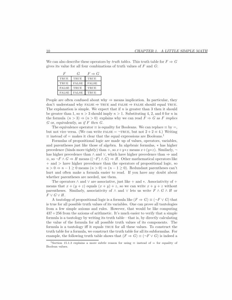
We can also describe these operators by truth tables. This truth table for F ⇒ Ggives its value for all four combinations of truth values of F and G:
F G F ⇒ Gtrue true truetrue false falsefalse true truefalse false true
People are often confused about why ⇒ means implication. In particular, theydon’t understand why false⇒ true and false⇒ false should equal true.The explanation is simple. We expect that if n is greater than 3 then it shouldbe greater than 1, so n > 3 should imply n > 1. Substituting 4, 2, and 0 for n inthe formula (n > 3)⇒ (n > 0) explains why we can read F ⇒ G as F impliesG or, equivalently, as if F then G.
The equivalence operator ≡ is equality for Booleans. We can replace ≡ by =,but not vice versa. (We can write false = ¬true, but not 2 + 2 ≡ 4.) Writing≡ instead of = makes it clear that the equal expressions are Booleans.1
Formulas of propositional logic are made up of values, operators, variables,and parentheses just like those of algebra. In algebraic formulas, ∗ has higherprecedence (binds more tightly) than +, so x+y∗z means x +(y∗z ). Similarly, ¬has higher precedence than ∧ and ∨, which have higher precedence than ⇒ and≡, so ¬F ∧G ⇒ H means ((¬F ) ∧G)⇒ H . Other mathematical operators like+ and > have higher precedence than the operators of propositional logic, son > 0⇒ n − 1 ≥ 0 means (n > 0)⇒ (n − 1 ≥ 0). Redundant parentheses can’thurt and often make a formula easier to read. If you have any doubt aboutwhether parentheses are needed, use them.
The operators ∧ and ∨ are associative, just like + and ∗. Associativity of +means that x + (y + z ) equals (x + y) + z , so we can write x + y + z withoutparentheses. Similarly, associativity of ∧ and ∨ lets us write F ∧ G ∧ H orF ∨G ∨H .
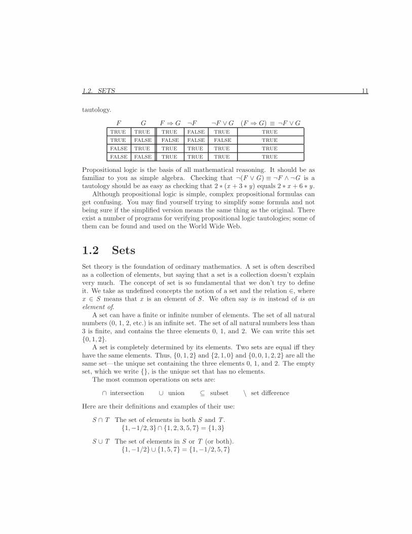
A tautology of propositional logic is a formula like (F ⇒ G) ≡ (¬F ∨G) thatis true for all possible truth values of its variables. One can prove all tautologiesfrom a few simple axioms and rules. However, that would be like computing437+256 from the axioms of arithmetic. It’s much easier to verify that a simpleformula is a tautology by writing its truth table—that is, by directly calculatingthe value of the formula for all possible truth values of its components. Theformula is a tautology iff it equals true for all these values. To construct thetruth table for a formula, we construct the truth table for all its subformulas. Forexample, the following truth table shows that (F ⇒ G) ≡ (¬F ∨G) is indeed a
1Section 15.1.3 explains a more subtle reason for using ≡ instead of = for equality ofBoolean values.
1.2. SETS 11
tautology.
F G F ⇒ G ¬F ¬F ∨G (F ⇒ G) ≡ ¬F ∨Gtrue true true false true truetrue false false false false truefalse true true true true truefalse false true true true true
Propositional logic is the basis of all mathematical reasoning. It should be asfamiliar to you as simple algebra. Checking that ¬(F ∨G) ≡ ¬F ∧ ¬G is atautology should be as easy as checking that 2 ∗ (x + 3 ∗ y) equals 2 ∗ x + 6 ∗ y .
Although propositional logic is simple, complex propositional formulas canget confusing. You may find yourself trying to simplify some formula and notbeing sure if the simplified version means the same thing as the original. Thereexist a number of programs for verifying propositional logic tautologies; some ofthem can be found and used on the World Wide Web.
1.2 Sets
Set theory is the foundation of ordinary mathematics. A set is often describedas a collection of elements, but saying that a set is a collection doesn’t explainvery much. The concept of set is so fundamental that we don’t try to defineit. We take as undefined concepts the notion of a set and the relation ∈, wherex ∈ S means that x is an element of S . We often say is in instead of is anelement of.
A set can have a finite or infinite number of elements. The set of all naturalnumbers (0, 1, 2, etc.) is an infinite set. The set of all natural numbers less than3 is finite, and contains the three elements 0, 1, and 2. We can write this set{0, 1, 2}.
A set is completely determined by its elements. Two sets are equal iff theyhave the same elements. Thus, {0, 1, 2} and {2, 1, 0} and {0, 0, 1, 2, 2} are all thesame set—the unique set containing the three elements 0, 1, and 2. The emptyset, which we write {}, is the unique set that has no elements.
The most common operations on sets are:
∩ intersection ∪ union ⊆ subset \ set difference
Here are their definitions and examples of their use:
S ∩ T The set of elements in both S and T .{1,−1/2, 3}∩ {1, 2, 3, 5, 7} = {1, 3}
S ∪ T The set of elements in S or T (or both).{1,−1/2} ∪ {1, 5, 7} = {1,−1/2, 5, 7}
12 CHAPTER 1. A LITTLE SIMPLE MATH
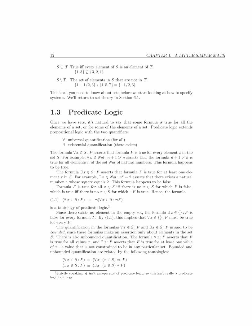
S ⊆ T True iff every element of S is an element of T .{1, 3} ⊆ {3, 2, 1}
S \T The set of elements in S that are not in T .{1,−1/2, 3} \ {1, 5, 7}= {−1/2, 3}
This is all you need to know about sets before we start looking at how to specifysystems. We’ll return to set theory in Section 6.1.
1.3 Predicate Logic
Once we have sets, it’s natural to say that some formula is true for all theelements of a set, or for some of the elements of a set. Predicate logic extendspropositional logic with the two quantifiers:
∀ universal quantification (for all)∃ existential quantification (there exists)
The formula ∀ x ∈ S : F asserts that formula F is true for every element x in theset S . For example, ∀n ∈ Nat : n + 1 > n asserts that the formula n + 1 > n istrue for all elements n of the set Nat of natural numbers. This formula happensto be true.
The formula ∃ x ∈ S : F asserts that formula F is true for at least one ele-ment x in S . For example, ∃n ∈ Nat : n2 = 2 asserts that there exists a naturalnumber n whose square equals 2. This formula happens to be false.
Formula F is true for all x ∈ S iff there is no x ∈ S for which F is false,which is true iff there is no x ∈ S for which ¬F is true. Hence, the formula
(∃ x ∈ S : F ) ≡ ¬(∀ x ∈ S :¬F )(1.1)
is a tautology of predicate logic.2
Since there exists no element in the empty set, the formula ∃ x ∈ {} : F isfalse for every formula F . By (1.1), this implies that ∀ x ∈ {} : F must be truefor every F .
The quantification in the formulas ∀ x ∈ S : F and ∃ x ∈ S : F is said to bebounded, since these formulas make an assertion only about elements in the setS . There is also unbounded quantification. The formula ∀ x : F asserts that Fis true for all values x , and ∃ x : F asserts that F is true for at least one valueof x—a value that is not constrained to be in any particular set. Bounded andunbounded quantification are related by the following tautologies:
(∀ x ∈ S : F ) ≡ (∀ x : (x ∈ S )⇒ F )(∃ x ∈ S : F ) ≡ (∃ x : (x ∈ S ) ∧ F )
2Strictly speaking, ∈ isn’t an operator of predicate logic, so this isn’t really a predicatelogic tautology.
1.3. PREDICATE LOGIC 13
The analog of (1.1) for unbounded quantifiers is also a tautology:
(∃ x : F ) ≡ ¬(∀ x :¬F )
Whenever possible, it is better to use bounded than unbounded quantificationin a specification. This makes the specification easier for both people and toolsto understand.
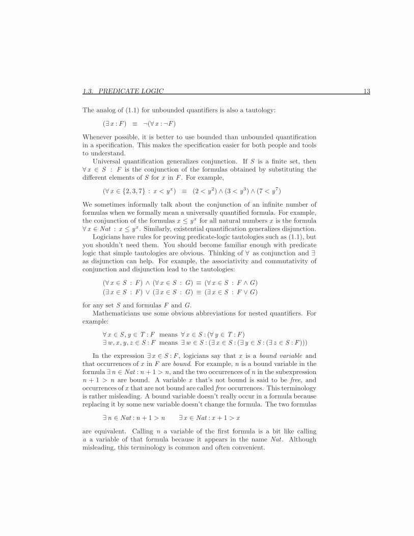
Universal quantification generalizes conjunction. If S is a finite set, then∀ x ∈ S : F is the conjunction of the formulas obtained by substituting thedifferent elements of S for x in F . For example,
(∀ x ∈ {2, 3, 7} : x < yx ) ≡ (2 < y2) ∧ (3 < y3) ∧ (7 < y7)
We sometimes informally talk about the conjunction of an infinite number offormulas when we formally mean a universally quantified formula. For example,the conjunction of the formulas x ≤ yx for all natural numbers x is the formula∀ x ∈ Nat : x ≤ yx . Similarly, existential quantification generalizes disjunction.
Logicians have rules for proving predicate-logic tautologies such as (1.1), butyou shouldn’t need them. You should become familiar enough with predicatelogic that simple tautologies are obvious. Thinking of ∀ as conjunction and ∃as disjunction can help. For example, the associativity and commutativity ofconjunction and disjunction lead to the tautologies:
(∀ x ∈ S : F ) ∧ (∀ x ∈ S : G) ≡ (∀ x ∈ S : F ∧G)(∃ x ∈ S : F ) ∨ (∃ x ∈ S : G) ≡ (∃ x ∈ S : F ∨G)
for any set S and formulas F and G.Mathematicians use some obvious abbreviations for nested quantifiers. For
example:
∀ x ∈ S , y ∈ T : F means ∀ x ∈ S : (∀ y ∈ T : F )∃w , x , y, z ∈ S : F means ∃w ∈ S : (∃ x ∈ S : (∃ y ∈ S : (∃ z ∈ S : F )))
In the expression ∃ x ∈ S : F , logicians say that x is a bound variable andthat occurrences of x in F are bound. For example, n is a bound variable in theformula ∃n ∈ Nat : n + 1 > n, and the two occurrences of n in the subexpressionn + 1 > n are bound. A variable x that’s not bound is said to be free, andoccurrences of x that are not bound are called free occurrences. This terminologyis rather misleading. A bound variable doesn’t really occur in a formula becausereplacing it by some new variable doesn’t change the formula. The two formulas
∃n ∈ Nat : n + 1 > n ∃ x ∈ Nat : x + 1 > x
are equivalent. Calling n a variable of the first formula is a bit like callinga a variable of that formula because it appears in the name Nat . Althoughmisleading, this terminology is common and often convenient.

14 CHAPTER 1. A LITTLE SIMPLE MATH
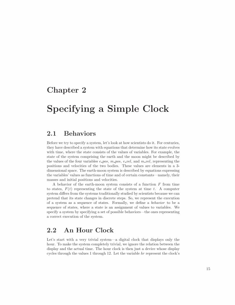
Chapter 2
Specifying a Simple Clock
2.1 Behaviors
Before we try to specify a system, let’s look at how scientists do it. For centuries,they have described a system with equations that determine how its state evolveswith time, where the state consists of the values of variables. For example, thestate of the system comprising the earth and the moon might be described bythe values of the four variables e pos , m pos , e vel , and m vel , representing thepositions and velocities of the two bodies. These values are elements in a 3-dimensional space. The earth-moon system is described by equations expressingthe variables’ values as functions of time and of certain constants—namely, theirmasses and initial positions and velocities.
A behavior of the earth-moon system consists of a function F from timeto states, F (t) representing the state of the system at time t . A computersystem differs from the systems traditionally studied by scientists because we canpretend that its state changes in discrete steps. So, we represent the executionof a system as a sequence of states. Formally, we define a behavior to be asequence of states, where a state is an assignment of values to variables. Wespecify a system by specifying a set of possible behaviors—the ones representinga correct execution of the system.
2.2 An Hour Clock
Let’s start with a very trivial system—a digital clock that displays only thehour. To make the system completely trivial, we ignore the relation between thedisplay and the actual time. The hour clock is then just a device whose displaycycles through the values 1 through 12. Let the variable hr represent the clock’s
15
16 CHAPTER 2. SPECIFYING A SIMPLE CLOCK
display. A typical behavior of the clock is the sequence
[hr = 11] → [hr = 12] → [hr = 1] → [hr = 2] → · · ·(2.1)
of states, where [hr = 11] is a state in which the variable hr has the value 11.A pair of successive states, such as [hr = 1]→ [hr = 2], is called a step.
To specify the hour clock, we describe all its possible behaviors. We write aninitial predicate that specifies the possible initial values of hr , and a next-staterelation that specifies how the value of hr can change in any step.
We don’t want to specify exactly what the display reads initially; any hourwill do. So, we want the initial predicate to assert that hr can have any valuefrom 1 through 12. Let’s call the initial predicate HCini . We might informallydefine HCini by:
HCini ∆= hr ∈ {1, . . . , 12}Later, we’ll see how to write this definition formally, without the “. . . ” thatstands for the informal and so on.
The next-state relation HCnxt is a formula expressing the relation betweenthe values of hr in the old (first) state and new (second) state of a step. Welet hr represent the value of hr in the old state and hr ′ represent its value inthe new state. (The ′ in hr ′ is read prime.) We want the next-state relation toassert that hr ′ equals hr + 1 except if hr equals 12, in which case hr ′ shouldequal 1. Using an if/then/else construct with the obvious meaning, we candefine HCnxt to be the next-state relation by writing:
HCnxt ∆= hr ′ = if hr 6= 12 then hr + 1 else 1
HCnxt is an ordinary mathematical formula, except that it contains primed aswell as unprimed variables. Such a formula is called an action. An action is trueor false of a step. A step that satisfies the action HCnxt is called an HCnxt step.
When an HCnxt step occurs, we sometimes say that HCnxt is executed.However, it would be a mistake to take this terminology seriously. An action isa formula, and formulas aren’t executed.
We want our specification to be a single formula, not the pair of formulasHCini and HCnxt . This formula must assert about a behavior that (i) its initialstate satisfies HCini , and (ii) each of its steps satisfies HCnxt . We express (i) asthe formula HCini , which we interpret as a statement about behaviors to meanthat the initial state satisfies HCini . To express (ii), we use the temporal-logicoperator 2 (pronounced box ). The temporal formula 2F asserts that formulaF is always true. In particular, 2HCnxt is the assertion that HCnxt is truefor every step in the behavior. So, HCini ∧ 2HCnxt is true of a behavior iffthe initial state satisfies HCini and every step satisfies HCnxt . This formuladescribes all behaviors like the one in (2.1) on this page; it seems to be thespecification we’re looking for.
2.2. AN HOUR CLOCK 17
If we considered the clock only in isolation, and never tried to relate it toanother system, then this would be a fine specification. However, suppose theclock is part of a larger system—for example, the hour display of a weatherstation that displays the current hour and temperature. The state of the sta-tion is described by two variables: hr , representing the hour display, and tmp,representing the temperature display. Consider this behavior of the weatherstation:[
hr = 11tmp = 23.5
]→
[hr = 12tmp = 23.5
]→
[hr = 12tmp = 23.4
]→
[hr = 12tmp = 23.3
]→
[hr = 1tmp = 23.3
]→ · · ·
In the second and third steps, tmp changes but hr remains the same. These stepsare not allowed by 2HCnxt , which asserts that every step must increment hr .The formula HCini ∧ 2HCnxt does not describe the hour clock in the weatherstation.
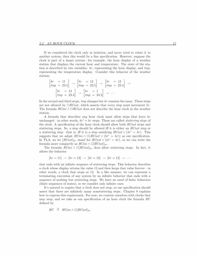
A formula that describes any hour clock must allow steps that leave hrunchanged—in other words, hr ′ = hr steps. These are called stuttering steps ofthe clock. A specification of the hour clock should allow both HCnxt steps andstuttering steps. So, a step should be allowed iff it is either an HCnxt step ora stuttering step—that is, iff it is a step satisfying HCnxt ∨ (hr ′ = hr). Thissuggests that we adopt HCini ∧ 2(HCnxt ∨ (hr ′ = hr)) as our specification.In TLA, we let [HCnxt ]hr stand for HCnxt ∨ (hr ′ = hr), so we can write theformula more compactly as HCini ∧ 2[HCnxt ]hr .
The formula HCini ∧ 2[HCnxt ]hr does allow stuttering steps. In fact, itallows the behavior
[hr = 11] → [hr = 12] → [hr = 12] → [hr = 12] → · · ·that ends with an infinite sequence of stuttering steps. This behavior describesa clock whose display attains the value 12 and then keeps that value forever—inother words, a clock that stops at 12. In a like manner, we can represent aterminating execution of any system by an infinite behavior that ends with asequence of nothing but stuttering steps. We have no need of finite behaviors(finite sequences of states), so we consider only infinite ones.
It’s natural to require that a clock does not stop, so our specification shouldassert that there are infinitely many nonstuttering steps. Chapter 8 explainshow to express this requirement. For now, we content ourselves with clocks thatmay stop, and we take as our specification of an hour clock the formula HCdefined by
HC ∆= HCini ∧ 2[HCnxt ]hr
18 CHAPTER 2. SPECIFYING A SIMPLE CLOCK
2.3 A Closer Look at the Hour-Clock Specifica-
tion
A state is an assignment of values to variables, but what variables? The answeris simple: all variables. In the behavior (2.1) on page 16, [hr = 1] representssome particular state that assigns the value 1 to hr . It might assign the value23 to the variable tmp and the value
√−17 to the variable m pos . We can thinkof a state as representing a potential state of the entire universe. A state thatassigns 1 to hr and a particular point in 3-space to m pos describes a state of theuniverse in which the hour clock reads 1 and the moon is in a particular place.A state that assigns
√−2 to hr doesn’t correspond to any state of the universethat we recognize, because the hour-clock can’t display the value
√−2. It mightrepresent the state of the universe after a bomb fell on the clock, making itsdisplay purely imaginary.
A behavior is an infinite sequence of states—for example:
[hr = 11] → [hr = 77.2] → [hr = 78.2] → [hr =√−2] → · · ·(2.2)
A behavior describes a potential history of the universe. The behavior (2.2)doesn’t correspond to a history that we understand, because we don’t know howthe clock’s display can change from 11 to 77.2. Whatever kind of history itrepresents is not one in which the clock is doing what it’s supposed to.
Formula HC is a temporal formula. A temporal formula is an assertionabout behaviors. We say that a behavior satisfies HC iff HC is a true assertionabout the behavior. Behavior (2.1) satisfies formula HC . Behavior (2.2) doesnot, because HC asserts that every step satisfies HCnxt , and the first and thirdsteps of (2.2) don’t. (The second step, [hr = 77.2] → [hr = 78.2], does satisfyHCnxt .) We regard formula HC to be the specification of an hour clock becauseit is satisfied by exactly those behaviors that represent histories of the universein which the clock functions properly.
If the clock is behaving properly, then its display should be an integer from 1through 12. So, hr should be an integer from 1 through 12 in every state of anybehavior satisfying the clock’s specification, HC . Formula HCini asserts thathr is an integer from 1 through 12, and 2HCini asserts that HCini is alwaystrue. So, 2HCini should be true for any behavior satisfying HC . Another wayof saying this is that HC implies 2HCini , for any behavior. Thus, the formulaHC ⇒ 2HCini should be satisfied by every behavior. A temporal formulasatisfied by every behavior is called a theorem, so HC ⇒ 2HCini should be atheorem.1 It’s easy to see that it is: HC implies that HCini is true initially (inthe first state of the behavior), and 2[HCnxt ]hr implies that each step eitheradvances hr to its proper next value or else leaves hr unchanged. We can
1Logicians call a formula valid if it is satisfied by every behavior; they reserve the termtheorem for provably valid formulas.
2.4. THE HOUR-CLOCK SPECIFICATION IN TLA+ 19
formalize this reasoning using the proof rules of TLA, but I’m not going todelve into proofs and proof rules.
2.4 The Hour-Clock Specification in TLA+
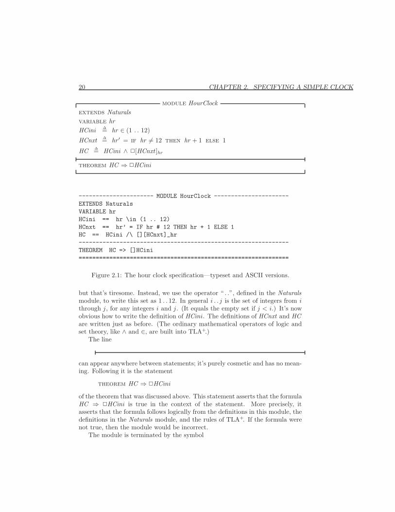
Figure 2.1 on the next page shows how the hour clock specification can be writtenin TLA+. There are two versions: the ascii version on the bottom is the actualTLA+ specification, the way you type it; the top version is typeset the way a“pretty-printer” might display it. Before trying to understand the specification,observe the relation between the two syntaxes:
• Reserved words that appear in small upper-case letters (like extends) arewritten in ascii with ordinary upper-case letters.
• When possible, symbols are represented pictorially in ascii—for example,2 is typed as [ ] and 6= as #. (You can also type 6= as /=.)
• When there is no good ascii representation, TEX notation [1] is used—forexample, ∈ is typed as \in.
A complete list of symbols and their ascii equivalents appears in Figure 13.16on page 243. I will usually show the typeset version of a specification; the asciiversions of all specifications appear in the Appendix.
Now let’s look at what the specification says. It starts with
module HourClock
which begins a module named HourClock . TLA+ specifications are partitionedinto modules; the hour clock’s specification consists of this single module.
Arithmetic operators like + are not built into TLA+, but are themselvesdefined in modules. (You might want to write a specification in which + meansaddition of matrices rather than numbers.) The usual operators on naturalnumbers are defined in the Naturals module. Their definitions are incorporatedinto module HourClock by the statement
extends Naturals
Every symbol that appears in a formula must either be a built-in operator ofTLA+, or else it must be declared or defined. The statement
variable hr
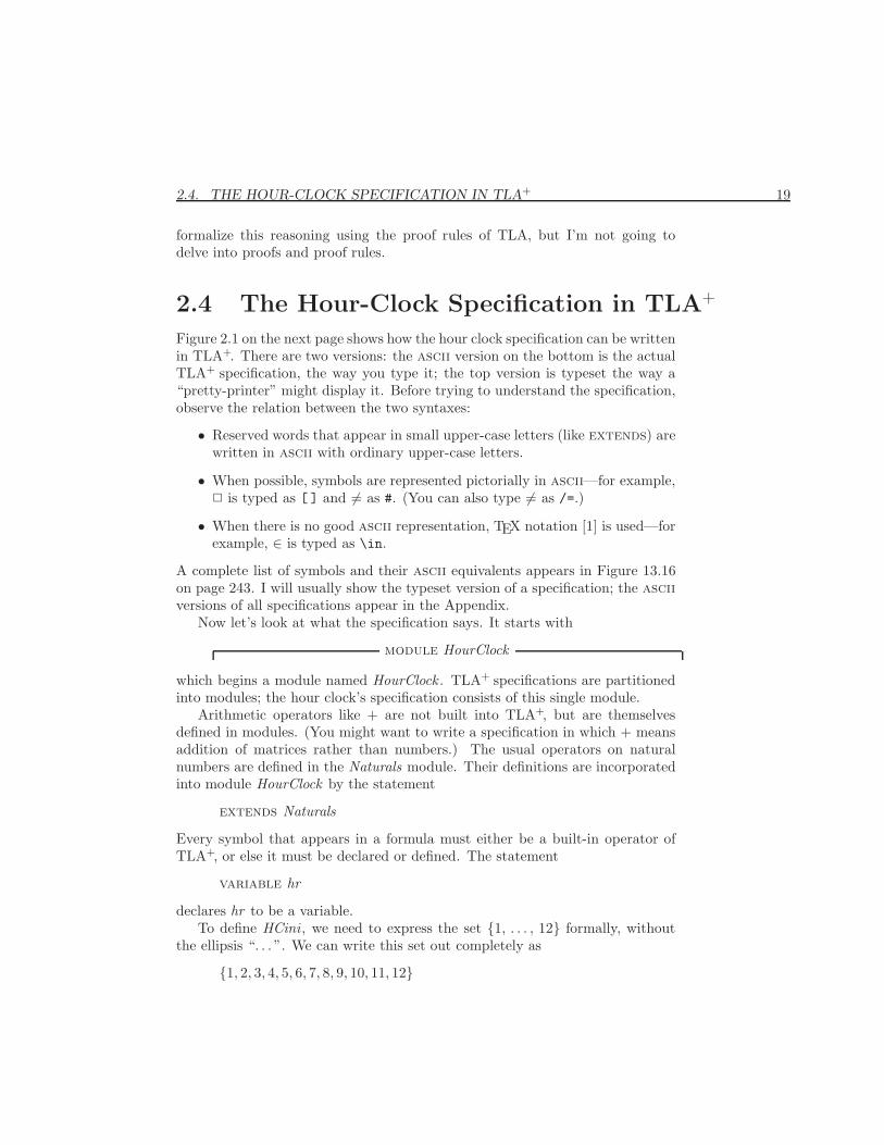
declares hr to be a variable.To define HCini , we need to express the set {1, . . . , 12} formally, without
the ellipsis “. . . ”. We can write this set out completely as
{1, 2, 3, 4, 5, 6, 7, 8, 9, 10, 11, 12}
20 CHAPTER 2. SPECIFYING A SIMPLE CLOCK
module HourClockextends Naturalsvariable hrHCini ∆= hr ∈ (1 . . 12)
HCnxt ∆= hr ′ = if hr 6= 12 then hr + 1 else 1
HC ∆= HCini ∧ 2[HCnxt ]hr
theorem HC ⇒ 2HCini
---------------------- MODULE HourClock ----------------------EXTENDS NaturalsVARIABLE hrHCini == hr \in (1 .. 12)HCnxt == hr’ = IF hr # 12 THEN hr + 1 ELSE 1HC == HCini /\ [][HCnxt]_hr--------------------------------------------------------------THEOREM HC => []HCini==============================================================
Figure 2.1: The hour clock specification—typeset and ASCII versions.
but that’s tiresome. Instead, we use the operator “ . .”, defined in the Naturalsmodule, to write this set as 1 . . 12. In general i . . j is the set of integers from ithrough j , for any integers i and j . (It equals the empty set if j < i .) It’s nowobvious how to write the definition of HCini . The definitions of HCnxt and HCare written just as before. (The ordinary mathematical operators of logic andset theory, like ∧ and ∈, are built into TLA+.)
The line
can appear anywhere between statements; it’s purely cosmetic and has no mean-ing. Following it is the statement
theorem HC ⇒ 2HCini
of the theorem that was discussed above. This statement asserts that the formulaHC ⇒ 2HCini is true in the context of the statement. More precisely, itasserts that the formula follows logically from the definitions in this module, thedefinitions in the Naturals module, and the rules of TLA+. If the formula werenot true, then the module would be incorrect.
The module is terminated by the symbol
2.5. ANOTHER WAY TO SPECIFY THE HOUR CLOCK 21
The specification of the hour clock is the definition of HC , including thedefinitions of the formulas HCnxt and HCini and of the operators . . and +that appear in the definition of HC . Formally, nothing in the module tells usthat HC rather than HCini is the clock’s specification. TLA+ is a language forwriting mathematics—in particular, for writing mathematical definitions andtheorems. What those definitions represent, and what significance we attach tothose theorems, lies outside the scope of mathematics and therefore outside thescope of TLA+. Engineering requires not just the ability to use mathematics,but the ability to understand what, if anything, the mathematics tells us aboutan actual system.
2.5 Another Way to Specify the Hour Clock
The Naturals module also defines the modulus operator, which we write %. Theformula i % n, which mathematicians write i mod n, is the remainder when i isdivided by n. More formally, i % n is the natural number less than n satisfyingi = q ∗ n + (i % n) for some natural number q. Let’s express this conditionmathematically. The Naturals module defines Nat to be the set of naturalnumbers, and the assertion that there exists a q in the set Nat satisfying aformula F is written ∃ q ∈ Nat : F . Thus, if i and n are elements of Nat andn > 0, then i % n is the unique number satisfying
(i % n ∈ 0 . . (n − 1)) ∧ (∃ q ∈ Nat : i = q ∗ n + (i % n))
We can use % to simplify our hour-clock specification a bit. Observing that(11 % 12)+1 equals 12 and (12 % 12)+1 equals 1, we can define a different next-state action HCnxt2 and a different formula HC2 to be the clock specification:
HCnxt2 ∆= hr ′ = (hr % 12) + 1 HC2 ∆= HCini ∧ 2[HCnxt2]hr
Actions HCnxt and HCnxt2 are not equivalent. The step [hr = 24]→ [hr = 25]satisfies HCnxt but not HCnxt2, while the step [hr = 24] → [hr = 1] satisfiesHCnxt2 but not HCnxt . However, any step starting in a state with hr in 1 . . 12satisfies HCnxt iff it satisfies HCnxt2. It’s therefore not hard to deduce that anybehavior starting in a state satisfying HCini satisfies 2[HCnxt ]hr iff it satisfies2[HCnxt2]hr . Hence, formulas HC and HC2 are equivalent. It doesn’t matterwhich of them we take to be the specification of an hour clock.
Mathematics provides infinitely many ways of expressing the same thing.The expressions 6 + 6, 3 ∗ 4, and 141− 129 all have the same meaning; they arejust different ways of writing the number 12. We could replace either instanceof the number 12 in module HourClock by any of these expressions withoutchanging the meaning of any of the module’s formulas.
22 CHAPTER 2. SPECIFYING A SIMPLE CLOCK
When writing a specification, you will often be faced with a choice of howto express something. When that happens, you should first make sure that thechoices yield equivalent specifications. If they do, then you can choose the onethat you feel makes the specification easiest to understand. If they don’t, thenyou must decide which one you mean.
Chapter 3
An Asynchronous Interface
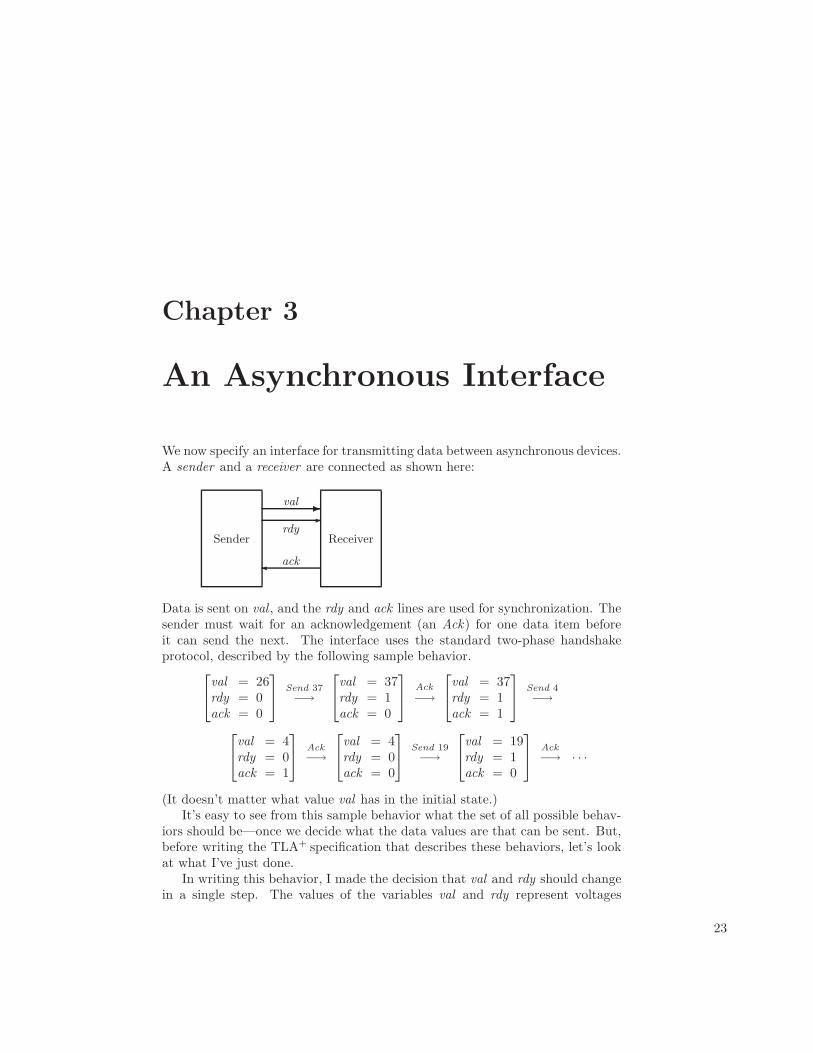
We now specify an interface for transmitting data between asynchronous devices.A sender and a receiver are connected as shown here:
Sender Receiver
val
rdy
--
ack�
Data is sent on val , and the rdy and ack lines are used for synchronization. Thesender must wait for an acknowledgement (an Ack) for one data item beforeit can send the next. The interface uses the standard two-phase handshakeprotocol, described by the following sample behavior.
val = 26rdy = 0ack = 0
Send 37−→
val = 37rdy = 1ack = 0
Ack
−→val = 37rdy = 1ack = 1
Send 4−→
val = 4rdy = 0ack = 1
Ack−→
val = 4rdy = 0ack = 0
Send 19−→
val = 19rdy = 1ack = 0
Ack−→ · · ·
(It doesn’t matter what value val has in the initial state.)It’s easy to see from this sample behavior what the set of all possible behav-
iors should be—once we decide what the data values are that can be sent. But,before writing the TLA+ specification that describes these behaviors, let’s lookat what I’ve just done.
In writing this behavior, I made the decision that val and rdy should changein a single step. The values of the variables val and rdy represent voltages
23
24 CHAPTER 3. AN ASYNCHRONOUS INTERFACE
on some set of wires in the physical device. Voltages on different wires don’tchange at precisely the same instant. I decided to ignore this aspect of thephysical system and pretend that the values of val and rdy represented by thosevoltages change instantaneously. This simplifies the specification, but at theprice of ignoring what may be an important detail of the system. In an actualimplementation of the protocol, the voltage on the rdy line shouldn’t changeuntil the voltages on the val lines have stabilized; but you won’t learn that frommy specification. Had I wanted the specification to convey this requirement, Iwould have written a behavior in which the value of val and the value of rdychange in separate steps.
A specification is an abstraction. It describes some aspects of the system andignores others. We want the specification to be as simple as possible, so we wantto ignore as many details as we can. But, whenever we omit some aspect of thesystem from the specification, we admit a potential source of error. With myspecification, we can verify the correctness of a system that uses this interface,and the system could still fail because the implementor didn’t know that the valline should stabilize before the rdy line is changed.
The hardest part of writing a specification is choosing the proper abstraction.I can teach you about TLA+, so expressing an abstract view of a system as aTLA+ specification becomes a straightforward task. But I don’t know how toteach you about abstraction. A good engineer knows how to abstract the essenceof a system and suppress the unimportant details when specifying and designingit. The art of abstraction is learned only through experience.
When writing a specification, you must first choose the abstraction. In aTLA+ specification, this means choosing (i) the variables that represent thesystem’s state and (ii) the granularity of the steps that change those variables’values. Should the rdy and ack lines be represented as separate variables oras a single variable? Should val and rdy change in one step, two steps, or anarbitrary number of steps? To help make these choices, I recommend that youstart by writing the first few steps of one or two sample behaviors, just as I didat the beginning of this section. Chapter 7 has more to say about these choices.
3.1 The First Specification
Now let’s specify the interface with a module AsynchInterface. The variablesrdy and ack can assume the values 0 and 1, which are natural numbers, soour module extends the Naturals module. We next decide what the possiblevalues of val should be—that is, what data values may be sent. We could writea specification that places no restriction on the data values. The specificationcould allow the sender to first send 37, then send
√−15, and then send Nat(the entire set of natural numbers). However, any real device can send only arestricted set of values. We could pick some specific set—for example, 32-bit
3.1. THE FIRST SPECIFICATION 25
numbers. However, the protocol is the same regardless of whether it’s used tosend 32-bit numbers or 128-bit numbers. So, we compromise between the twoextremes of allowing anything to be sent and allowing only 32-bit numbers tobe sent by assuming only that there is some set Data of data values that maybe sent. The constant Data is a parameter of the specification. It’s declared bythe statement
constant Data
Our three variables are declared by
variables val , rdy, ack
The keywords variable and variables are synonymous, as are constant andconstants.
The variable rdy can assume any value—for example, −1/2. That is, thereexist states that assign the value −1/2 to rdy. When discussing the specification,we usually say that rdy can assume only the values 0 and 1. What we really meanis that the value of rdy equals 0 or 1 in every state of any behavior satisfying thespecification. But a reader of the specification shouldn’t have to understand thecomplete specification to figure this out. We can make the specification easierto understand by telling the reader what values the variables can assume in abehavior that satisfies the specification. We could do this with comments, but Iprefer to use a definition like this one:
TypeInvariant ∆= (val ∈ Data) ∧ (rdy ∈ {0, 1}) ∧ (ack ∈ {0, 1})I call the set {0, 1} the type of rdy, and I call TypeInvariant a type invariant.Let’s define type and some other terms more precisely:
• A state function is an ordinary expression (one with no prime or 2) thatcan contain variables and constants.
• A state predicate is a Boolean-valued state function.
• An invariant Inv of a specification Spec is a state predicate such thatSpec ⇒ 2Inv is a theorem.
• A variable v has type T in a specification Spec iff v ∈ T is an invariant ofSpec.
We can make the definition of TypeInvariant easier to read by writing it asfollows.
TypeInvariant ∆= ∧ val ∈ Data∧ rdy ∈ {0, 1}∧ ack ∈ {0, 1}
26 CHAPTER 3. AN ASYNCHRONOUS INTERFACE
Each conjunct begins with a ∧ and must lie completely to the right of that∧. (The conjunct may occupy multiple lines). We use a similar notation fordisjunctions. When using this bulleted-list notation, the ∧’s or ∨’s must line upprecisely (even in the ascii input). Because the indentation is significant, we caneliminate parentheses, making this notation especially useful when conjunctionsand disjunctions are nested.
The formula TypeInvariant will not appear as part of the specification. Wedo not assume that TypeInvariant is an invariant; the specification should implythat it is. In fact, its invariance will be asserted as a theorem.
The initial predicate is straightforward. Initially, val can equal any elementof Data. We can start with rdy and ack either both 0 or both 1.
Init ∆= ∧ val ∈ Data∧ rdy ∈ {0, 1}∧ ack = rdy
Now for the next-state action Next . A step of the protocol either sends a valueor receives a value. We define separately the two actions Send and Rcv thatdescribe the sending and receiving of a value. A Next step (one satisfying actionNext) is either a Send step or a Rcv step, so it is a Send ∨Rcv step. Therefore,Next is defined to equal Send ∨Rcv . Let’s now define Send and Rcv .
We say that action Send is enabled in a state from which it is possible totake a Send step. From the sample behavior above, we see that Send is enablediff rdy equals ack . Usually, the first question we ask about an action is, whenis it enabled? So, the definition of an action usually begins with its enablingcondition. The first conjunct in the definition of Send is therefore rdy = ack .The next conjuncts tell us what the new values of the variables val , rdy, andack are. The new value val ′ of val can be any element of Data—that is, anyvalue satisfying val ′ ∈ Data. The value of rdy changes from 0 to 1 or from 1 to0, so rdy ′ equals 1− rdy (because 1 = 1− 0 and 0 = 1− 1). The value of ack isleft unchanged.
TLA+ defines unchanged v to mean that the expression v has the samevalue in the old and new states. More precisely, unchanged v equals v ′ = v ,where v ′ is the expression obtained from v by priming all variables. So, wedefine Send by:
Send ∆= ∧ rdy = ack∧ val ′ ∈ Data∧ rdy ′ = 1− rdy∧ unchanged ack
(I could have written ack ′ = ack instead of unchanged ack , but I prefer to usethe unchanged construct in specifications.)
A Rcv step is enabled iff rdy is different from ack ; it complements the valueof ack and leaves val and rdy unchanged. Both val and rdy are left unchanged iff
3.1. THE FIRST SPECIFICATION 27
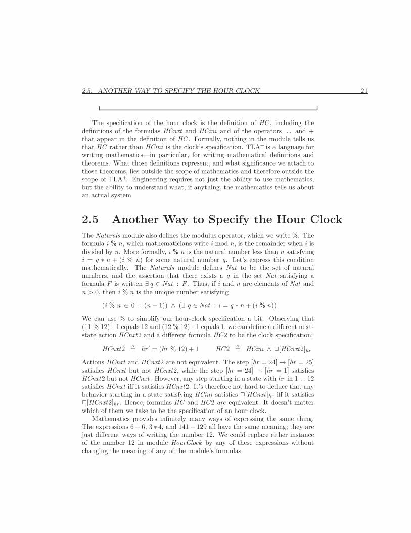
module AsynchInterface
extends Naturalsconstant Datavariables val , rdy, ackTypeInvariant ∆= ∧ val ∈ Data
∧ rdy ∈ {0, 1}∧ ack ∈ {0, 1}
Init ∆= ∧ val ∈ Data∧ rdy ∈ {0, 1}∧ ack = rdy
Send ∆= ∧ rdy = ack∧ val ′ ∈ Data∧ rdy ′ = 1− rdy∧ unchanged ack
Rcv ∆= ∧ rdy 6= ack∧ ack ′ = 1− ack∧ unchanged 〈val , rdy 〉
Next ∆= Send ∨ RcvSpec ∆= Init ∧ 2[Next ]〈val,rdy,ack 〉
theorem Spec ⇒ 2TypeInvariant
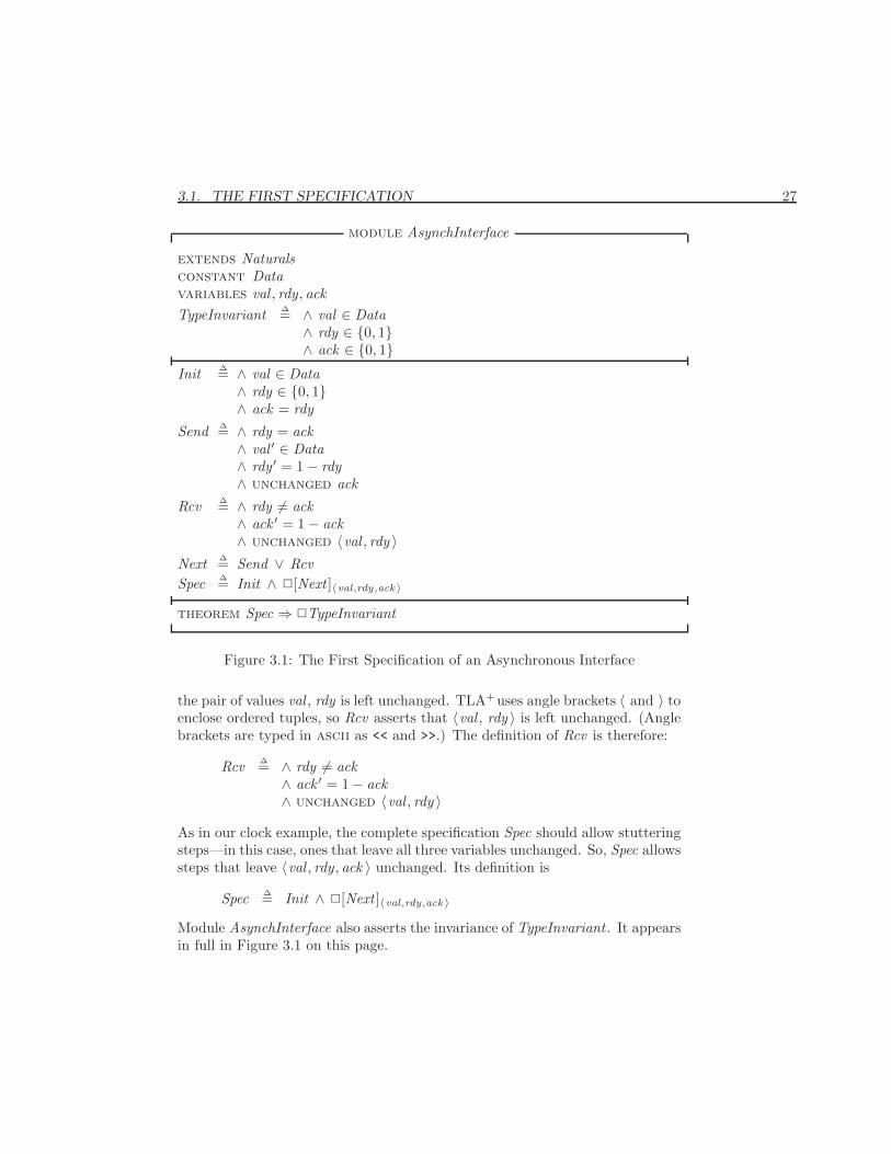
Figure 3.1: The First Specification of an Asynchronous Interface
the pair of values val , rdy is left unchanged. TLA+uses angle brackets 〈 and 〉 toenclose ordered tuples, so Rcv asserts that 〈val , rdy 〉 is left unchanged. (Anglebrackets are typed in ascii as << and >>.) The definition of Rcv is therefore:
Rcv ∆= ∧ rdy 6= ack∧ ack ′ = 1− ack∧ unchanged 〈val , rdy 〉
As in our clock example, the complete specification Spec should allow stutteringsteps—in this case, ones that leave all three variables unchanged. So, Spec allowssteps that leave 〈val , rdy, ack 〉 unchanged. Its definition is
Spec ∆= Init ∧ 2[Next ]〈val,rdy,ack 〉
Module AsynchInterface also asserts the invariance of TypeInvariant . It appearsin full in Figure 3.1 on this page.
28 CHAPTER 3. AN ASYNCHRONOUS INTERFACE
3.2 Another Specification
Module AsynchInterface is a fine description of the interface and its handshakeprotocol. However, it’s not easy to use it to help specify a system that uses theinterface. Let’s rewrite the interface specification in a form that makes it moreconvenient to use as part of a larger specification.
The first problem with the original specification is that it uses three variablesto describe a single interface. A system might use several different instances ofthe interface. To avoid a proliferation of variables, we replace the three variablesval , rdy, ack with a single variable chan (short for channel). A mathematicianwould do this by letting the value of chan be an ordered triple—for example, astate [chan = 〈−1/2, 0, 1〉] might replace the state with val = −1/2, rdy = 0,and ack = 1. But programmers have learned that using tuples like this leads tomistakes; it’s easy to forget if the ack line is represented by the second or thirdcomponent. TLA+ therefore provides records in addition to more conventionalmathematical notation.
Let’s represent the state of the channel as a record with val , rdy, and ackfields. If r is such a record, then r .val is its val field. The type invariant assertsthat the value of chan is an element of the set of all such records r in whichr .val is an element of the set Data and r .rdy and r .ack are elements of the set{0, 1}. This set of records is written:
[val : Data, rdy : {0, 1}, ack : {0, 1}]The components of a record are not ordered, so it doesn’t matter in what orderwe write them. This same set of records can also be written as:
[ack : {0, 1}, val : Data, rdy : {0, 1}]Initially, chan can equal any element of this set whose ack and rdy fields areequal, so the initial predicate is the conjunction of the type invariant and thecondition chan.ack = chan.rdy.
A system that uses the interface may perform an operation that sends somedata value d and performs some other changes that depend on the value d .We’d like to represent such an operation as an action that is the conjunctionof two separate actions: one that describes the sending of d and the other thatdescribes the other changes. Thus, instead of defining an action Send that sendssome unspecified data value, we define the action Send(d) that sends data valued . The next-state action is satisfied by a Send(d) step, for some d in Data, ora Rcv step. (The value received by a Rcv step equals chan.val .) Saying thata step is a Send(d) step for some d in Data means that there exists a d inData such that the step satisfies Send(d)—in other words, that the step is an∃ d ∈ Data : Send(d) step. So we define
Next ∆= (∃ d ∈ Data : Send(d)) ∨ Rcv
3.2. ANOTHER SPECIFICATION 29
The Send(d) action asserts that chan ′ equals the record r such that:
r .val = d r .rdy = 1− chan.rdy r .ack = chan.ack
This record is written in TLA+ as:
[val 7→ d , rdy 7→ 1− chan.rdy, ack 7→ chan.ack ]
(The symbol 7→ is typed in ascii as |-> .) The fields of records are not ordered,so this record can just as well be written:
[ack 7→ chan.ack , val 7→ d , rdy 7→ 1− chan.rdy]
The enabling condition of Send(d) is that the rdy and ack lines are equal, so wecan define:
Send(d) ∆=∧ chan.rdy = chan.ack∧ chan ′ = [val 7→ d , rdy 7→ 1− chan.rdy, ack 7→ chan.ack ]
This is a perfectly good definition of Send(d). However, I prefer a slightlydifferent one. We can describe the value of chan ′ by saying that it is the same asthe value of chan except that its val component equals d and its rdy componentequals 1− chan.rdy. In TLA+, we can write this value as
[chan except !.val = d , !.rdy = 1− chan.rdy]
Think of the ! as standing for the new record that the except expression formsby modifying chan. So, the expression can be read as the record ! that isthe same as chan except ! .val equals d and !.rdy equals 1 − chan.rdy. In theexpression that !.rdy equals, the symbol @ stands for chan.rdy, so we can writethis except expression as:
[chan except !.val = d , !.rdy = 1−@]
In general, for any record r , the expression
[r except !.c1 = e1, . . . , !.cn = en ]
is the record obtained from r by replacing r .ci with ei , for each i in 1 . . n. An@ in the expression ei stands for r .ci . Using this notation, we define:
Send(d) ∆= ∧ chan.rdy = chan.ack∧ chan ′ = [chan except !.val = d , !.rdy = 1−@]
The definition of Rcv is straightforward. A value can be received when chan.rdy 6=chan.ack , and receiving the value complements chan.ack :
Rcv ∆= ∧ chan.rdy 6= chan.ack∧ chan ′ = [chan except !.ack = 1−@]
30 CHAPTER 3. AN ASYNCHRONOUS INTERFACE
module Channel
extends Naturalsconstant Datavariable chanTypeInvariant ∆= chan ∈ [val : Data, rdy : {0, 1}, ack : {0, 1}]
Init ∆= ∧ TypeInvariant∧ chan.ack = chan.rdy
Send(d) ∆= ∧ chan.rdy = chan.ack∧ chan ′ = [chan except !.val = d , !.rdy = 1−@]
Rcv ∆= ∧ chan.rdy 6= chan.ack∧ chan ′ = [chan except !.ack = 1−@]
Next ∆= (∃ d ∈ Data : Send(d)) ∨ Rcv
Spec ∆= Init ∧ 2[Next ]chan
theorem Spec ⇒ 2TypeInvariant
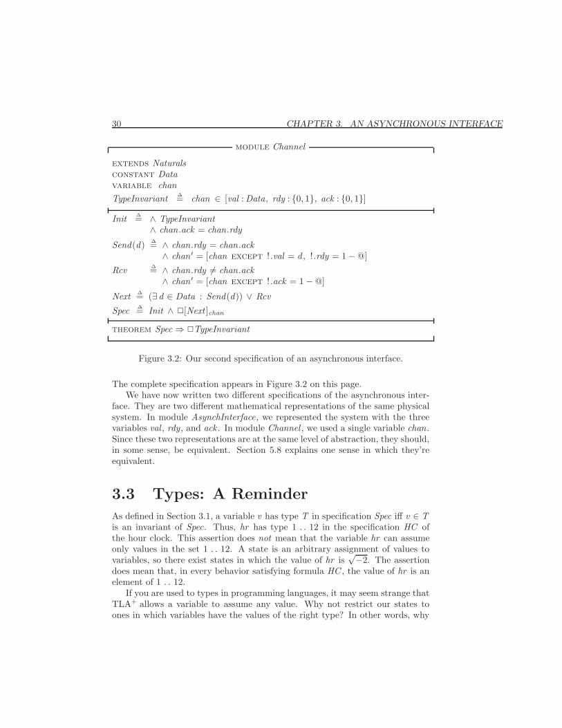
Figure 3.2: Our second specification of an asynchronous interface.
The complete specification appears in Figure 3.2 on this page.We have now written two different specifications of the asynchronous inter-
face. They are two different mathematical representations of the same physicalsystem. In module AsynchInterface, we represented the system with the threevariables val , rdy, and ack . In module Channel , we used a single variable chan.Since these two representations are at the same level of abstraction, they should,in some sense, be equivalent. Section 5.8 explains one sense in which they’reequivalent.
3.3 Types: A Reminder
As defined in Section 3.1, a variable v has type T in specification Spec iff v ∈ Tis an invariant of Spec. Thus, hr has type 1 . . 12 in the specification HC ofthe hour clock. This assertion does not mean that the variable hr can assumeonly values in the set 1 . . 12. A state is an arbitrary assignment of values tovariables, so there exist states in which the value of hr is
√−2. The assertiondoes mean that, in every behavior satisfying formula HC , the value of hr is anelement of 1 . . 12.
If you are used to types in programming languages, it may seem strange thatTLA+ allows a variable to assume any value. Why not restrict our states toones in which variables have the values of the right type? In other words, why
3.4. DEFINITIONS 31
not add a formal type system to TLA+? A complete answer would take us toofar afield. The question is addressed further in Section 6.2. For now, rememberthat TLA+ is an untyped language. Type correctness is just a name for a certaininvariance property. Assigning the name TypeInvariant to a formula gives it nospecial status.
3.4 Definitions
Let’s examine what a definition means. If Id is a simple identifier like Initor Spec, then the definition Id ∆= exp defines Id to be synonymous with theexpression exp. Replacing Id by exp, or vice-versa, in any expression e does notchange the meaning of e. This replacement must be done after the expressionis parsed, not in the “raw input”. For example, the definition x ∆= a + b makesx ∗ c equal to (a + b) ∗ c, not to a + b ∗ c, which equals a + (b ∗ c).
The definition of Send has the form Id(p) ∆= exp, where Id and p are identi-fiers. For any expression e, this defines Id(e) to be the expression obtained bysubstituting e for p in exp. For example, the definition of Send in the Channelmodule defines Send(−5) to equal
∧ chan.rdy = chan.ack∧ chan ′ = [chan except !.val = −5, !.rdy = 1−@]
Send(e) is an expression, for any expression e. Thus, we can write the formulaSend(−5) ∧ (chan.ack = 1). The identifier Send by itself is not an expression,and Send ∧ (chan.ack = 1) is not a grammatically well-formed string. It’s non-syntactic nonsense, like a + ∗ b + .
We say that Send is an operator that takes a single argument. We defineoperators that take more than one argument in the obvious way, the generalform being:
Id(p1, . . . , pn) ∆= exp(3.1)
where the pi are distinct identifiers and exp is an expression. We can considerdefined identifiers like Init and Spec to be operators that take no argument, butwe generally use operator to mean an operator that takes one or more arguments.
I will use the term symbol to mean an identifier like Send or an operatorsymbol like +. Every symbol that is used in a specification must either be a built-in operator of TLA+ (like ∈) or it must be declared or defined. Every symboldeclaration or definition has a scope within which the symbol may be used. Thescope of a variable or constant declaration, and of a definition, is the part ofthe module that follows it. Thus, we can use Init in any expression that followsits definition in module Channel . The statement extends Naturals extends thescope of symbols like + defined in the Naturals module to the Channel module.
32 CHAPTER 3. AN ASYNCHRONOUS INTERFACE
The operator definition (3.1) implicitly includes a declaration of the identi-fiers p1, . . . , pn whose scope is the expression exp. An expression of the form
∃ v ∈ S : exp
has a declaration of v whose scope is the expression exp. Thus the identifier vhas a meaning within the expression exp (but not within the expression S ).
A symbol cannot be declared or defined if it already has a meaning. Theexpression
(∃ v ∈ S : exp1) ∧ (∃ v ∈ T : exp2)
is all right, because neither declaration of v lies within the scope of the other.Similarly, the two declarations of the symbol d in the Channel module (in thedefinition of Send and in the expression ∃ d in the definition of Next) havedisjoint scopes. However, the expression
(∃ v ∈ S : (exp1 ∧ ∃ v ∈ T : exp2))
is illegal because the declaration of v in the second ∃ v lies inside the scopeof the its declaration in the first ∃ v . Although conventional mathematics andprogramming languages allow such redeclarations, TLA+ forbids them becausethey can lead to confusion and errors.
3.5 Comments
Even simple specifications like the ones in modules AsynchInterface and Channelcan be hard to understand from the mathematics alone. That’s why I began withan intuitive explanation of the interface. That explanation made it easier foryou to understand formula Spec in the module, which is the actual specification.Every specification should be accompanied by an informal prose explanation.The explanation may be in an accompanying document, or it may be includedas comments in the specification.
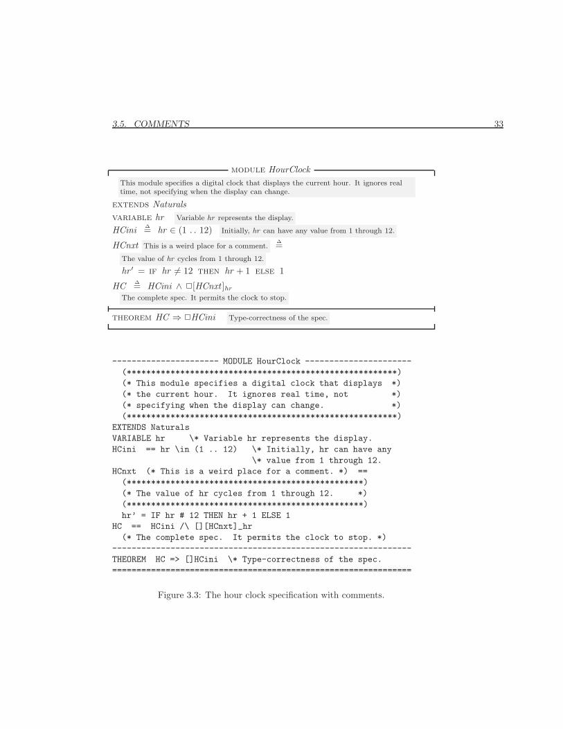
Figure 3.3 on the next page shows how the hour clock’s specification inmodule HourClock might be explained by comments. In the typeset version,comments are distinguished from the specification itself by the use of a differentfont. As shown in the figure, TLA+ provides two way of writing comments inthe ascii version. A comment may appear anywhere enclosed between (* and*). The text of the comment itself may not contain *), so these comments can’tbe nested. An end-of-line comment is preceded by \*.
A comment almost always appears on a line by itself or at the end of a line.I put a comment between HCnxt and ∆= just to show that it can be done.
To save space, I will write few comments in the example specifications. Butspecifications should have lots of comments. Even if there is an accompany-ing document describing the system, comments are needed to help the readerunderstand how the specification formalizes that description.
3.5. COMMENTS 33
module HourClockThis module specifies a digital clock that displays the current hour. It ignores realtime, not specifying when the display can change.
extends Naturalsvariable hr Variable hr represents the display.
HCini ∆= hr ∈ (1 . . 12) Initially, hr can have any value from 1 through 12.
HCnxt This is a weird place for a comment.∆=
The value of hr cycles from 1 through 12.
hr ′ = if hr 6= 12 then hr + 1 else 1
HC ∆= HCini ∧ 2[HCnxt ]hrThe complete spec. It permits the clock to stop.
theorem HC ⇒ 2HCini Type-correctness of the spec.
---------------------- MODULE HourClock ----------------------(********************************************************)(* This module specifies a digital clock that displays *)(* the current hour. It ignores real time, not *)(* specifying when the display can change. *)(********************************************************)
EXTENDS NaturalsVARIABLE hr \* Variable hr represents the display.HCini == hr \in (1 .. 12) \* Initially, hr can have any
\* value from 1 through 12.HCnxt (* This is a weird place for a comment. *) ==(*************************************************)(* The value of hr cycles from 1 through 12. *)(*************************************************)hr’ = IF hr # 12 THEN hr + 1 ELSE 1
HC == HCini /\ [][HCnxt]_hr(* The complete spec. It permits the clock to stop. *)
--------------------------------------------------------------THEOREM HC => []HCini \* Type-correctness of the spec.==============================================================
Figure 3.3: The hour clock specification with comments.
34 CHAPTER 3. AN ASYNCHRONOUS INTERFACE
Comments can help solve a problem posed by the logical structure of a spec-ification. A symbol has to be declared or defined before it can be used. Inmodule Channel , the definition of Spec has to follow the definition of Next ,which has to follow the definitions of Send and Rcv . But it’s usually easiest tounderstand a top-down description of a system. We would probably first wantto read the declarations of Data and chan, then the definition of Spec, thenthe definitions of Init and Next , and then the definitions of Send and Rcv . Inother words, we want to read the specification more or less from bottom to top.This is easy enough to do for a module as short as Channel ; it’s inconvenientfor longer specifications. We can use comments to guide the reader through alonger specification. For example, we could precede the definition of Send in theChannel module with the comment:
Actions Send and Rcv below are the disjuncts of the next-state actionNext .
The module structure also allows us to choose the order in which a spec-ification is read. For example, we can rewrite the hour-clock specification bysplitting the HourClock module into three separate modules:
HCVar A module that declares the variable hr .
HCActions A module that extends modules Naturals and HCVar and de-fines HCini and HCnxt .
HCSpec A module that extends module HCActions , defines formulaHC , and asserts the type-correctness theorem.
The extends relation implies a logical ordering of the modules: HCVar precedesHCActions , which precedes HCSpec. But the modules don’t have to be read inthat order. The reader can be told to read HCVar first, then HCSpec, and finallyHCActions . The instance construct introduced below in Chapter 4 providesanother tool for modularizing specifications.
Splitting a tiny specification like HourClock in this way would be ludicrous.But the proper splitting of modules can help make a large specification easier toread. When writing a specification, you should decide in what order it shouldbe read. You can then design the module structure to permit reading it in thatorder, when each individual module is read from beginning to end. Finally,you should ensure that the comments within each module make sense when thedifferent modules are read in the appropriate order.
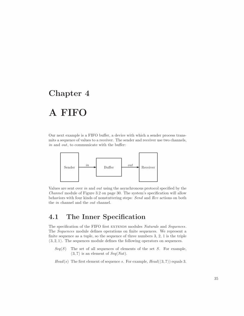
Chapter 4
A FIFO
Our next example is a FIFO buffer, a device with which a sender process trans-mits a sequence of values to a receiver. The sender and receiver use two channels,in and out , to communicate with the buffer:
Sender Buffer Receiverin out- -
Values are sent over in and out using the asynchronous protocol specified by theChannel module of Figure 3.2 on page 30. The system’s specification will allowbehaviors with four kinds of nonstuttering steps: Send and Rcv actions on boththe in channel and the out channel.
4.1 The Inner Specification
The specification of the FIFO first extends modules Naturals and Sequences .The Sequences module defines operations on finite sequences. We represent afinite sequence as a tuple, so the sequence of three numbers 3, 2, 1 is the triple〈3, 2, 1〉. The sequences module defines the following operators on sequences.
Seq(S ) The set of all sequences of elements of the set S . For example,〈3, 7〉 is an element of Seq(Nat).
Head(s) The first element of sequence s . For example, Head(〈3, 7〉) equals 3.
35
36 CHAPTER 4. A FIFO
Tail(s) The tail of sequence s (all but the head of s). For example, Tail(〈3, 7〉)equals 〈7〉.
Append(s , e) The sequence obtained by appending element e to the tail ofsequence s . For example, Append(〈3, 7〉, 3) equals 〈3, 7, 3〉.
s ◦ t The sequence obtained by concatenating the sequences s and t . Forexample, 〈3, 7〉 ◦ 〈3〉 equals 〈3, 7, 3〉. (We type ◦ in ascii as \o.)
Len(s) The length of sequence s . For example, Len(〈3, 7〉) equals 2.
The FIFO’s specification continues by declaring the constant Message, whichrepresents the set of all messages that can be sent.1 It then declares the variables.There are three variables: in and out , representing the channels, and a thirdvariable q that represents the queue of buffered messages. The value of q is thesequence of messages that have been sent by the sender but not yet received bythe receiver. (Section 4.3 has more to say about this additional variable q.)
We want to use the definitions in the Channel module to specify operations The Channelmodule appearsin Figure 3.2 onpage 30.
on the channels in and out . This requires two instances of that module—onein which the variable chan of the Channel module is replaced with the variablein of our current module, and the other in which chan is replaced with out .In both instances, the constant Data of the Channel module is replaced withMessage. We obtain the first of these instances with the statement:
InChan ∆= instance Channel with Data ← Message, chan ← in
For every symbol σ defined in module Channel , this defines InChan !σ to havethe same meaning in the current module as σ had in module Channel , exceptwith Message substituted for Data and in substituted for chan. For example,this statement defines InChan !TypeInvariant to equal
in ∈ [val : Message, rdy : {0, 1}, ack : {0, 1}](The statement does not define InChan !Data because Data is declared, notdefined, in module Channel .) We introduce our second instance of the Channelmodule with the analogous statement:
OutChan ∆= instance Channel with Data ← Message,chan ← out
The initial states of the in and out channels are specified by InChan !Init andOutChan !Init . Initially, no messages have been sent or received, so q should
1I like to use a singular noun like Message rather than a plural like Messages for the nameof a set. That way, the ∈ in the expression m ∈ Message can be read is a. This is the sameconvention that most programmers use for naming types.
4.2. INSTANTIATION EXAMINED 37
equal the empty sequence. The empty sequence is the zero-tuple (there’s onlyone, and it’s written 〈 〉), so we define the initial predicate to be:
Init ∆= ∧ InChan !Init∧ OutChan !Init∧ q = 〈 〉
We next define the type invariant. The type invariants for in and out come fromthe Channel module, and the type of q is the set of finite sequences of messages.The type invariant for the FIFO specification is therefore:
TypeInvariant ∆= ∧ InChan !TypeInvariant∧ OutChan !TypeInvariant∧ q ∈ Seq(Message)
The four kinds of nonstuttering steps allowed by the next-state action are de-scribed by four actions:
SSend(msg) The sender sends message msg on the in channel.
BufRcv The buffer receives the message from the in channel and ap-pends it to the tail of q.
BufSend The buffer removes the message from the head of q and sendsit on channel out .
RRcv The receiver receives the message from the out channel.
The definitions of these actions, along with the rest of the specification, are inmodule InnerFIFO of Figure 4.1 on the next page. The reason for the adjectiveInner is explained in Section 4.3 below.
4.2 Instantiation Examined
4.2.1 Instantiation is Substitution
Consider the definition of Next in module Channel (page 30). We can removeevery defined symbol that appears in that definition by using the symbol’s defi-nition. For example, we can eliminate the expression Send(d) by expanding thedefinition of Send . We can repeat this process. For example the − that appearsin the expression 1 − @ (obtained by expanding the definition of Send) can beeliminated by using the definition of − from the Naturals module. Continuing inthis way, we eventually obtain a definition for Next in terms of only the built-inoperators of TLA+ and the parameters Data and chan of the Channel module.
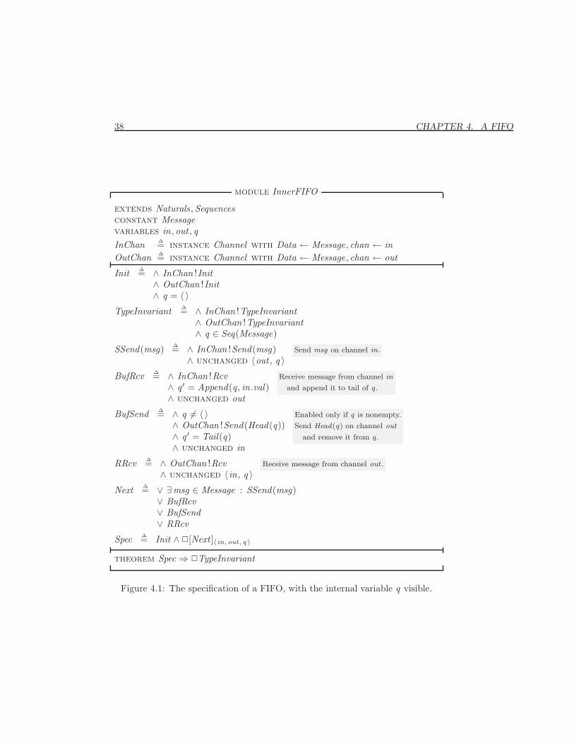
38 CHAPTER 4. A FIFO
module InnerFIFO
extends Naturals ,Sequencesconstant Messagevariables in, out , qInChan ∆= instance Channel with Data ← Message, chan ← inOutChan ∆= instance Channel with Data ← Message, chan ← out
Init ∆= ∧ InChan !Init∧ OutChan !Init∧ q = 〈 〉
TypeInvariant ∆= ∧ InChan !TypeInvariant∧ OutChan !TypeInvariant∧ q ∈ Seq(Message)
SSend(msg) ∆= ∧ InChan !Send(msg)∧ unchanged 〈out , q 〉
Send msg on channel in.
BufRcv ∆= ∧ InChan !Rcv∧ q ′ = Append(q, in.val)∧ unchanged out
Receive message from channel in
and append it to tail of q .
BufSend ∆= ∧ q 6= 〈 〉∧ OutChan !Send(Head(q))∧ q ′ = Tail(q)∧ unchanged in
Enabled only if q is nonempty.
Send Head(q) on channel out
and remove it from q .
RRcv ∆= ∧ OutChan !Rcv∧ unchanged 〈in, q 〉
Receive message from channel out .
Next ∆= ∨ ∃msg ∈ Message : SSend(msg)∨ BufRcv∨ BufSend∨ RRcv
Spec ∆= Init ∧ 2[Next ]〈in,out, q 〉
theorem Spec ⇒ 2TypeInvariant
Figure 4.1: The specification of a FIFO, with the internal variable q visible.
4.2. INSTANTIATION EXAMINED 39
We consider this to be the “real” definition of Next in module Channel . Thestatement
InChan ∆= instance Channel with Data ← Message, chan ← in
in module InnerFIFO defines InChan !Next to be the formula obtained fromthis real definition of Next by substituting Message for Data and in for chan.This defines InChan !Next in terms of only the built-in operators of TLA+ andthe parameters Message and in of module InnerFIFO .
Let’s now consider an arbitrary instance statement
IM ∆= instance M with p1 ← e1, . . . , pn ← en
Let Σ be a symbol defined in module M and let d be its “real” definition. Theinstance statement defines IM !Σ to have as its real definition the expressionobtained from d by replacing all instances of pi by the expression ei , for each i .The definition of IM !Σ must contain only the parameters (declared constantsand variables) of the current module, not the ones of module M . Hence, the pi
must consist of all the parameters of module M . The ei must be expressionsthat are meaningful in the current module.
4.2.2 Parametrized Instantiation
The FIFO specification uses two instances of module Channel—one with insubstituted for chan and the other with out substituted for chan. We couldinstead use a single parametrized instance by putting the following statement inmodule InnerFIFO :
Chan(ch) ∆= instance Channel with Data ← Message, chan ← ch
For any symbol Σ defined in module Channel and any expression exp, this de-fines Chan(exp)!Σ to equal formula Σ with Message substituted for Data andexp substituted for chan. The Rcv action on channel in could then be writ-ten Chan(in)!Rcv , and the Send(msg) action on channel out could be writtenChan(out)!Send(msg).
The instantiation above defines Chan !Send to be an operator with two argu-ments. Writing Chan(out)!Send(msg) instead of Chan !Send(out ,msg) is justan idiosyncrasy of the syntax. It is no stranger than the syntax for infix opera-tors, which makes us write a + b instead of +(a, b).
4.2.3 Implicit Substitutions
The use of Message as the name for the set of transmitted values in the FIFOspecification is a bit strange, since we had just used the name Data for the
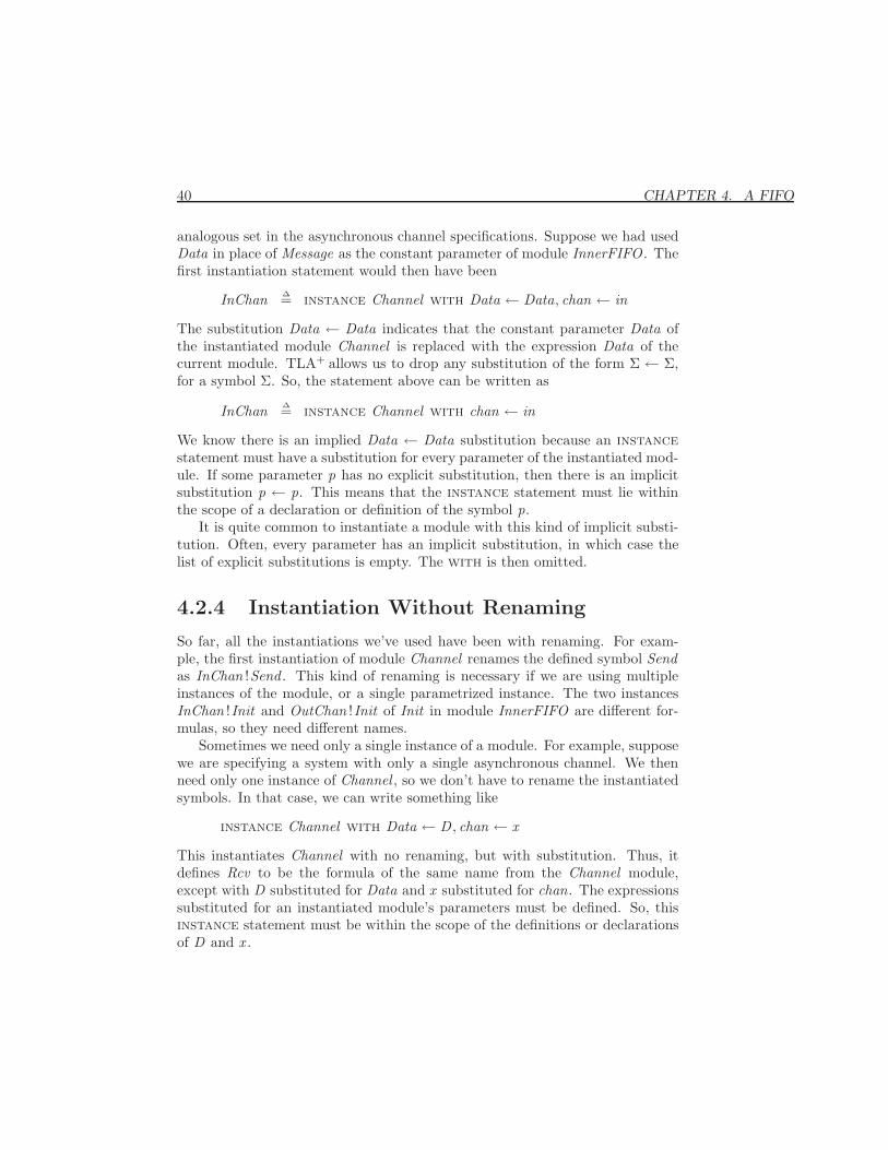
40 CHAPTER 4. A FIFO
analogous set in the asynchronous channel specifications. Suppose we had usedData in place of Message as the constant parameter of module InnerFIFO . Thefirst instantiation statement would then have been
InChan ∆= instance Channel with Data ← Data, chan ← in
The substitution Data ← Data indicates that the constant parameter Data ofthe instantiated module Channel is replaced with the expression Data of thecurrent module. TLA+ allows us to drop any substitution of the form Σ ← Σ,for a symbol Σ. So, the statement above can be written as
InChan ∆= instance Channel with chan ← in
We know there is an implied Data ← Data substitution because an instancestatement must have a substitution for every parameter of the instantiated mod-ule. If some parameter p has no explicit substitution, then there is an implicitsubstitution p ← p. This means that the instance statement must lie withinthe scope of a declaration or definition of the symbol p.
It is quite common to instantiate a module with this kind of implicit substi-tution. Often, every parameter has an implicit substitution, in which case thelist of explicit substitutions is empty. The with is then omitted.
4.2.4 Instantiation Without Renaming
So far, all the instantiations we’ve used have been with renaming. For exam-ple, the first instantiation of module Channel renames the defined symbol Sendas InChan !Send . This kind of renaming is necessary if we are using multipleinstances of the module, or a single parametrized instance. The two instancesInChan !Init and OutChan !Init of Init in module InnerFIFO are different for-mulas, so they need different names.
Sometimes we need only a single instance of a module. For example, supposewe are specifying a system with only a single asynchronous channel. We thenneed only one instance of Channel , so we don’t have to rename the instantiatedsymbols. In that case, we can write something like
instance Channel with Data ← D , chan ← x
This instantiates Channel with no renaming, but with substitution. Thus, itdefines Rcv to be the formula of the same name from the Channel module,except with D substituted for Data and x substituted for chan. The expressionssubstituted for an instantiated module’s parameters must be defined. So, thisinstance statement must be within the scope of the definitions or declarationsof D and x .
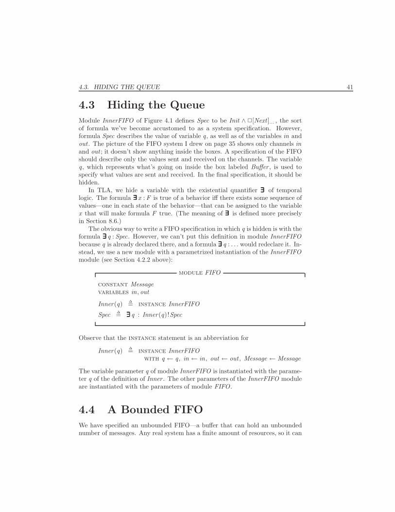
4.3. HIDING THE QUEUE 41
4.3 Hiding the Queue
Module InnerFIFO of Figure 4.1 defines Spec to be Init ∧ 2[Next ]... , the sortof formula we’ve become accustomed to as a system specification. However,formula Spec describes the value of variable q, as well as of the variables in andout . The picture of the FIFO system I drew on page 35 shows only channels inand out ; it doesn’t show anything inside the boxes. A specification of the FIFOshould describe only the values sent and received on the channels. The variableq, which represents what’s going on inside the box labeled Buffer , is used tospecify what values are sent and received. In the final specification, it should behidden.
In TLA, we hide a variable with the existential quantifier ∃∃∃∃∃∃ of temporallogic. The formula ∃∃∃∃∃∃ x : F is true of a behavior iff there exists some sequence ofvalues—one in each state of the behavior—that can be assigned to the variablex that will make formula F true. (The meaning of ∃∃∃∃∃∃ is defined more preciselyin Section 8.6.)
The obvious way to write a FIFO specification in which q is hidden is with theformula ∃∃∃∃∃∃ q : Spec. However, we can’t put this definition in module InnerFIFObecause q is already declared there, and a formula ∃∃∃∃∃∃ q : . . . would redeclare it. In-stead, we use a new module with a parametrized instantiation of the InnerFIFOmodule (see Section 4.2.2 above):
module FIFO
constant Messagevariables in, out
Inner(q) ∆= instance InnerFIFO
Spec ∆= ∃∃∃∃∃∃ q : Inner(q)!Spec
Observe that the instance statement is an abbreviation for
Inner(q) ∆= instance InnerFIFOwith q ← q, in ← in, out ← out , Message ← Message
The variable parameter q of module InnerFIFO is instantiated with the parame-ter q of the definition of Inner . The other parameters of the InnerFIFO moduleare instantiated with the parameters of module FIFO .
4.4 A Bounded FIFO
We have specified an unbounded FIFO—a buffer that can hold an unboundednumber of messages. Any real system has a finite amount of resources, so it can
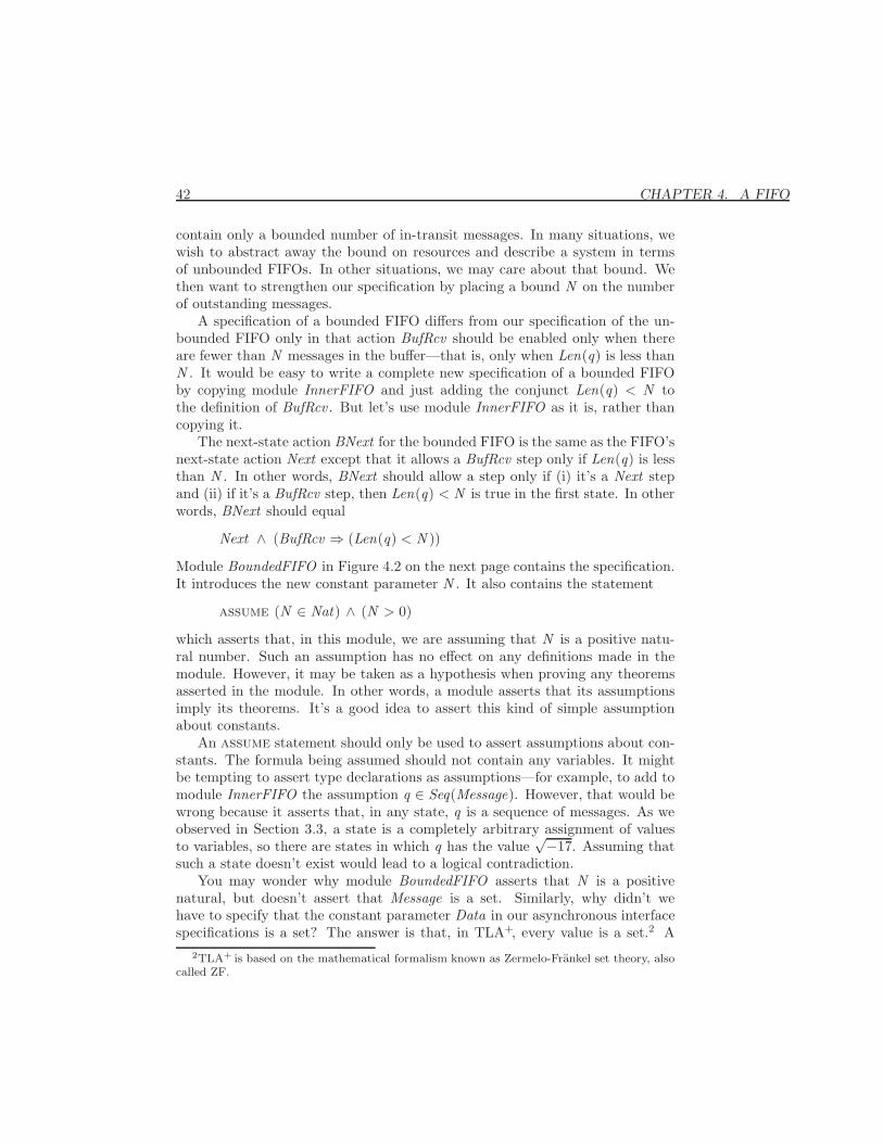
42 CHAPTER 4. A FIFO
contain only a bounded number of in-transit messages. In many situations, wewish to abstract away the bound on resources and describe a system in termsof unbounded FIFOs. In other situations, we may care about that bound. Wethen want to strengthen our specification by placing a bound N on the numberof outstanding messages.
A specification of a bounded FIFO differs from our specification of the un-bounded FIFO only in that action BufRcv should be enabled only when thereare fewer than N messages in the buffer—that is, only when Len(q) is less thanN . It would be easy to write a complete new specification of a bounded FIFOby copying module InnerFIFO and just adding the conjunct Len(q) < N tothe definition of BufRcv . But let’s use module InnerFIFO as it is, rather thancopying it.
The next-state action BNext for the bounded FIFO is the same as the FIFO’snext-state action Next except that it allows a BufRcv step only if Len(q) is lessthan N . In other words, BNext should allow a step only if (i) it’s a Next stepand (ii) if it’s a BufRcv step, then Len(q) < N is true in the first state. In otherwords, BNext should equal
Next ∧ (BufRcv ⇒ (Len(q) < N ))
Module BoundedFIFO in Figure 4.2 on the next page contains the specification.It introduces the new constant parameter N . It also contains the statement
assume (N ∈ Nat) ∧ (N > 0)
which asserts that, in this module, we are assuming that N is a positive natu-ral number. Such an assumption has no effect on any definitions made in themodule. However, it may be taken as a hypothesis when proving any theoremsasserted in the module. In other words, a module asserts that its assumptionsimply its theorems. It’s a good idea to assert this kind of simple assumptionabout constants.
An assume statement should only be used to assert assumptions about con-stants. The formula being assumed should not contain any variables. It mightbe tempting to assert type declarations as assumptions—for example, to add tomodule InnerFIFO the assumption q ∈ Seq(Message). However, that would bewrong because it asserts that, in any state, q is a sequence of messages. As weobserved in Section 3.3, a state is a completely arbitrary assignment of valuesto variables, so there are states in which q has the value
√−17. Assuming thatsuch a state doesn’t exist would lead to a logical contradiction.
You may wonder why module BoundedFIFO asserts that N is a positivenatural, but doesn’t assert that Message is a set. Similarly, why didn’t wehave to specify that the constant parameter Data in our asynchronous interfacespecifications is a set? The answer is that, in TLA+, every value is a set.2 A
2TLA+ is based on the mathematical formalism known as Zermelo-Frankel set theory, alsocalled ZF.
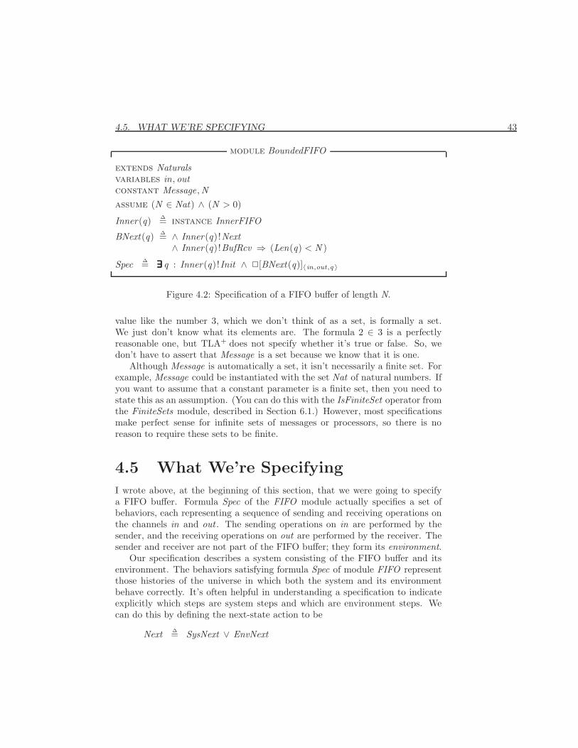
4.5. WHAT WE’RE SPECIFYING 43
module BoundedFIFO
extends Naturalsvariables in, outconstant Message,Nassume (N ∈ Nat) ∧ (N > 0)
Inner(q) ∆= instance InnerFIFO
BNext(q) ∆= ∧ Inner(q)!Next∧ Inner(q)!BufRcv ⇒ (Len(q) < N )
Spec ∆= ∃∃∃∃∃∃ q : Inner(q)!Init ∧ 2[BNext(q)]〈in,out,q 〉
Figure 4.2: Specification of a FIFO buffer of length N.
value like the number 3, which we don’t think of as a set, is formally a set.We just don’t know what its elements are. The formula 2 ∈ 3 is a perfectlyreasonable one, but TLA+ does not specify whether it’s true or false. So, wedon’t have to assert that Message is a set because we know that it is one.
Although Message is automatically a set, it isn’t necessarily a finite set. Forexample, Message could be instantiated with the set Nat of natural numbers. Ifyou want to assume that a constant parameter is a finite set, then you need tostate this as an assumption. (You can do this with the IsFiniteSet operator fromthe FiniteSets module, described in Section 6.1.) However, most specificationsmake perfect sense for infinite sets of messages or processors, so there is noreason to require these sets to be finite.
4.5 What We’re Specifying
I wrote above, at the beginning of this section, that we were going to specifya FIFO buffer. Formula Spec of the FIFO module actually specifies a set ofbehaviors, each representing a sequence of sending and receiving operations onthe channels in and out . The sending operations on in are performed by thesender, and the receiving operations on out are performed by the receiver. Thesender and receiver are not part of the FIFO buffer; they form its environment.
Our specification describes a system consisting of the FIFO buffer and itsenvironment. The behaviors satisfying formula Spec of module FIFO representthose histories of the universe in which both the system and its environmentbehave correctly. It’s often helpful in understanding a specification to indicateexplicitly which steps are system steps and which are environment steps. Wecan do this by defining the next-state action to be
Next ∆= SysNext ∨ EnvNext
44 CHAPTER 4. A FIFO
where SysNext describes system steps and EnvNext describes environment steps.For the FIFO, we have
SySNext ∆= BufRcv ∨ BufSend
EnvNext ∆= (∃msg ∈ Message : SSend(msg)) ∨ RRcv
While suggestive, this way of defining the next-state action has no formal sig-nificance. The specification Spec equals Init ∧ 2[Next ]... ; changing the way westructure the definition of Next doesn’t change its meaning. If a behavior failsto satisfy Spec, nothing tells us if the system or its environment is to blame.
A formula like Spec, which describes the correct behavior of both the systemand its environment, is called a closed-system or complete-system specification.An open-system specification is one that describes only the correct behavior ofthe system. A behavior satisfies an open-system specification if it represents ahistory in which either the system operates correctly, or it failed to operate cor-rectly only because its environment did something wrong. Section 10.7 explainshow to write open-system specifications.
Open-system specifications are philosophically more satisfying. However,closed-system specifications are a little bit easier to write, and the mathematicsunderlying them is simpler. So, we almost always write closed-system speci-fications. It’s usually quite easy to turn a closed-system specification into anopen-system specification. But in practice, there’s little reason to do so.
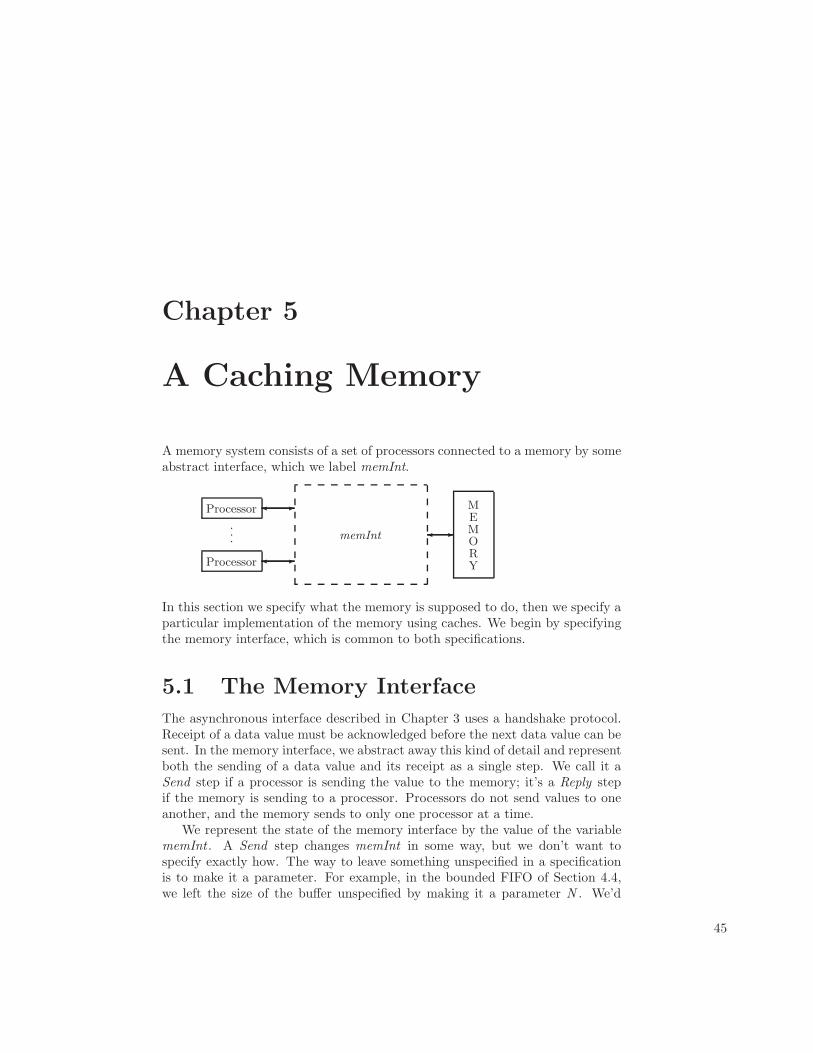
Chapter 5
A Caching Memory
A memory system consists of a set of processors connected to a memory by someabstract interface, which we label memInt.
Processor
Processor
-�
-�
-�p
p
p
memInt
MEMORY
In this section we specify what the memory is supposed to do, then we specify aparticular implementation of the memory using caches. We begin by specifyingthe memory interface, which is common to both specifications.
5.1 The Memory Interface
The asynchronous interface described in Chapter 3 uses a handshake protocol.Receipt of a data value must be acknowledged before the next data value can besent. In the memory interface, we abstract away this kind of detail and representboth the sending of a data value and its receipt as a single step. We call it aSend step if a processor is sending the value to the memory; it’s a Reply stepif the memory is sending to a processor. Processors do not send values to oneanother, and the memory sends to only one processor at a time.
We represent the state of the memory interface by the value of the variablememInt . A Send step changes memInt in some way, but we don’t want tospecify exactly how. The way to leave something unspecified in a specificationis to make it a parameter. For example, in the bounded FIFO of Section 4.4,we left the size of the buffer unspecified by making it a parameter N . We’d
45
46 CHAPTER 5. A CACHING MEMORY
therefore like to declare a parameter Send so that Send(p, d) describes howmemInt is changed by a step that represents processor p sending data valued to the memory. However, TLA+ provides only constant and variableparameters, not action parameters.1 So, we declare Send to be a constantoperator and write Send(p, d ,memInt ,memInt ′) instead of Send(p, d).
In TLA+, we declare Send to be a constant operator that takes four argu-ments by writing
constant Send( , , , )
This means that Send(p, d ,miOld ,miNew) is an expression, for any expressionsp, d , miOld , and miNew , but it says nothing about what the value of thatexpression is. We want it to be a Boolean value that is true iff a step in whichmemInt equals miOld in the first state and miNew in the second state representsthe sending by p of value d to the memory.2 We can assert that the value is aBoolean by the assumption:
assume ∀ p, d , miOld , miNew :Send(p, d ,miOld ,miNew) ∈ boolean
This asserts that the formula
Send(p, d ,miOld ,miNew) ∈ boolean
is true for all values of p, d , miOld , and miNew . The built-in symbol booleandenotes the set {true, false}, whose elements are the two Boolean values trueand false.
This assume statement asserts formally that the value of
Send(p, d ,miOld ,miNew)
is a Boolean. But the only way to assert formally what that value signifies wouldbe to say what it actually equals—that is, to define Send rather than makingit a parameter. We don’t want to do that, so we just state informally whatthe value means. This statement is part of the intrinsically informal descriptionof the relation between our mathematical abstraction and a physical memorysystem.
To allow the reader to understand the specification, we have to describeinformally what Send means. The assume statement asserting that Send(. . .)is a Boolean is then superfluous as an explanation. However, it could help toolsunderstand the specification, so it’s a good idea to include it anyway.
1Even if TLA+ allowed us to declare an action parameter, we would have no way to specifythat a Send(p, d) action constrains only memInt and not other variables.
2We expect Send(p, d ,miOld , miNew) to have this meaning only when p is a processor andd a value that p is allowed to send, but we simplify the specification a bit by requiring it tobe a Boolean for all values of p and d .
5.1. THE MEMORY INTERFACE 47
A specification that uses the memory interface can use the operators Sendand Reply to specify how the variable memInt changes. The specification mustalso describe memInt ’s initial value. We therefore declare a constant parameterInitMemInt that is the set of possible initial values of memInt .
We also introduce three constant parameters that are needed to describe theinterface:
Proc The set of processor identifiers. (We usually shorten processor identifierto processor when referring to an element of Proc.)
Adr The set of memory addresses.
Val The set of possible memory values that can be assigned to an address.
Finally, we define the values that the processors and memory send to one anotherover the interface. A processor sends a request to the memory. We representa request as a record with an op field that specifies the type of request andadditional fields that specify its arguments. Our simple memory allows justread and write requests. A read request has op field “Rd” and an adr fieldspecifying the address to be read. The set of all read requests is therefore theset
[op : {“Rd”}, adr : Adr ]
of all records whose op field equals “Rd” (is an element of the set {“Rd”} whoseonly element is the string “Rd”) and whose adr field is an element of Adr . Awrite request must specify the address to be written and the value to write. It isrepresented by a record with op field equal to “Wr”, and with adr and val fieldsspecifying the address and value. We define MReq, the set of all requests, toequal the union of these two sets. (Set operations, including union, are describedin Section 1.2.)
The memory responds to a read request with the memory value it read.We will also have it respond to a write request; and it seems nice to let theresponse be different from the response to any read request. We therefore requirethe memory to respond to a write request by returning a value NoVal that isdifferent from any memory value. We could declare NoVal to be a constantparameter and add the assumption NoVal /∈ Val . (The symbol /∈ is typed inascii as \notin .) But it’s best, when possible, to avoid introducing parameters.Instead, we define NoVal by:
NoVal ∆= choose v : v /∈ Val
The expression choose x : F equals an arbitrarily chosen value x that satisfiesthe formula F . (If no such x exists, the expression has a completely arbitraryvalue.) This statement defines NoVal to be some value that is not an element of
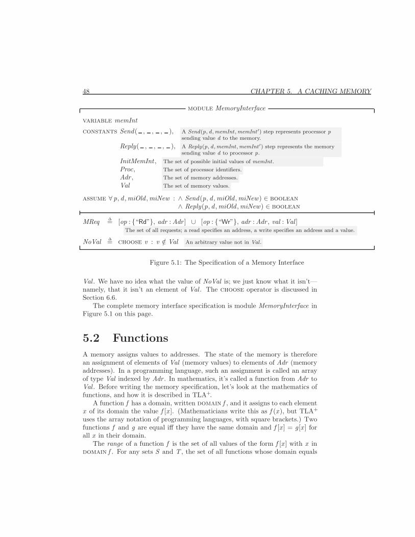
48 CHAPTER 5. A CACHING MEMORY
module MemoryInterface
variable memInt
constants Send( , , , ), A Send(p, d , memInt , memInt ′) step represents processor psending value d to the memory.
Reply( , , , ), A Reply(p, d ,memInt , memInt ′) step represents the memorysending value d to processor p.
InitMemInt , The set of possible initial values of memInt .
Proc, The set of processor identifiers.
Adr , The set of memory addresses.
Val The set of memory values.
assume ∀ p, d ,miOld ,miNew : ∧ Send(p, d ,miOld ,miNew) ∈ boolean∧ Reply(p, d ,miOld ,miNew) ∈ boolean
MReq ∆= [op : {“Rd”}, adr : Adr ] ∪ [op : {“Wr”}, adr : Adr , val : Val ]The set of all requests; a read specifies an address, a write specifies an address and a value.
NoVal ∆= choose v : v /∈ Val An arbitrary value not in Val .
Figure 5.1: The Specification of a Memory Interface
Val . We have no idea what the value of NoVal is; we just know what it isn’t—namely, that it isn’t an element of Val . The choose operator is discussed inSection 6.6.
The complete memory interface specification is module MemoryInterface inFigure 5.1 on this page.
5.2 Functions
A memory assigns values to addresses. The state of the memory is thereforean assignment of elements of Val (memory values) to elements of Adr (memoryaddresses). In a programming language, such an assignment is called an arrayof type Val indexed by Adr . In mathematics, it’s called a function from Adr toVal . Before writing the memory specification, let’s look at the mathematics offunctions, and how it is described in TLA+.
A function f has a domain, written domain f , and it assigns to each elementx of its domain the value f [x ]. (Mathematicians write this as f (x ), but TLA+
uses the array notation of programming languages, with square brackets.) Twofunctions f and g are equal iff they have the same domain and f [x ] = g[x ] forall x in their domain.
The range of a function f is the set of all values of the form f [x ] with x indomain f . For any sets S and T , the set of all functions whose domain equals
5.2. FUNCTIONS 49
S and whose range is any subset of T is written [S → T ].Ordinary mathematics does not have a convenient notation for writing an ex-
pression whose value is a function. TLA+ defines [x ∈ S 7→ e] to be the functionf with domain S such that f [x ] = e for every x ∈ S .3 For example,
succ ∆= [n ∈ Nat 7→ n + 1]
defines succ to be the successor function on the natural numbers—the functionwith domain Nat such that succ[n] = n + 1 for all n ∈ Nat .
A record is a function whose domain is a finite set of strings. For example,a record with val , ack , and rdy fields is a function whose domain is the set{“val”, “ack”, “rdy”} consisting of the three strings “val”, “ack”, and “rdy”.The expression r .ack , the ack field of a record r , is an abbreviation for r [“ack”].The record
[val 7→ 42, ack 7→ 1, rdy 7→ 0]
can be written
[i ∈ {“val”, “ack”, “rdy”} 7→if i = “val” then 42 else if i = “ack” then 1 else 0]
The except construct for records, explained in Section 3.2, is a special case of ageneral except construct for functions, where !.c is an abbreviation for ![“c”].For any function f , the expression [f except ! [c] = e] is the function f that isthe same as f except with f [c] = e. This function can also be written:
[x ∈ domain f 7→ if x = c then e else f [x ] ]
assuming that the symbol x does not occur in any of the expressions f , c, ande. For example, [succ except ! [42] = 86] is the function g that is the same assucc except that g[42] equals 86 instead of 43.
As in the except construct for records, the expression e in
[f except ! [c] = e]
can contain the symbol @, where it means f [c]. For example,
[succ except ! [42] = 2 ∗@] = [succ except ! [42] = 2 ∗ succ[42] ]
In general,
[f except ! [c1] = e1, . . . , ! [cn ] = en ]
3The ∈ in [x ∈ S 7→ e] is just part of the syntax; TLA+ uses that particular symbol to helpyou remember what the construct means. Computer scientists write λx : S .e to representsomething similar to [x ∈ S 7→ e], except that their λ expressions aren’t quite the same as thefunctions of ordinary mathematics that are used in TLA+.
50 CHAPTER 5. A CACHING MEMORY
is the function f that is the same as f except with f [ci ] = ei for each i . Moreprecisely, this expression equals
[. . . [ [f except ! [c1] = e1] except ! [c2] = e2] . . . except ! [cn ] = en ]
Functions correspond to the arrays of programming languages. The domain of afunction corresponds to the index set of an array. The function [f except ! [c] = e]corresponds to the array obtained from f by assigning e to f [c]. A function whoserange is a set of functions corresponds to an array of arrays. TLA+ defines[f except ! [c][d ] = e] to be the function corresponding to the array obtainedby assigning e to f [c][d ]. It can be written as
[f except ! [c] = [@ except ! [d ] = e]]
The generalization to [f except ! [c1] . . . [cn ] = e] for any n should be obvious.Since a record is a function, this notation can be used for records as well. TLA+
uniformly maintains the notation that σ.c is an abbreviation for σ[“c”]. Forexample, this implies:
[f except ! [c].d = e] = [f except ! [c] = [@ except !.d = e]]
The TLA+ definition of records as functions makes it possible to manipulatethem in ways that have no counterparts in programming languages. For example,we can define an operator R such that R(r , s) is the record obtained from r byreplacing the value of each field c that is also a field of the record s with s .c.In other words, for every field c of r , if c is a field of s then R(r , s).c = s .c;otherwise R(r , s).c = r .c. The definition is:
R(r , s) ∆= [c ∈ domain r 7→ if c ∈ domain s then s [c] else r [c] ]
So far, I have described only functions of a single argument. TLA+ alsoallows functions of multiple arguments. Section 15.1.7 on page 275 describes thegeneral versions of the TLA+ function constructs for functions with any numberof arguments. However, functions of a single argument are all you really need.You can always replace a function of multiple arguments with a function-valuedfunction—for example, writing f [a][b] instead of f [a, b].
5.3 A Linearizable Memory Specification
We specify a very simple memory system in which a processor p issues a mem-ory request and then waits for a response before issuing the next request. Inour specification, the request is executed by accessing (reading or modifying) avariable mem, which represents the current state of the memory. Because thememory can receive requests from other processors before responding to pro-cessor p, it matters when mem is accessed. We let the access of mem occur
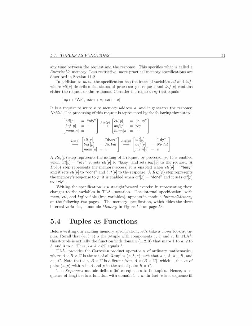
5.4. TUPLES AS FUNCTIONS 51
any time between the request and the response. This specifies what is called alinearizable memory. Less restrictive, more practical memory specifications aredescribed in Section 11.2.
In addition to mem, the specification has the internal variables ctl and buf ,where ctl [p] describes the status of processor p’s request and buf [p] containseither the request or the response. Consider the request req that equals
[op 7→ “Wr”, adr 7→ a, val 7→ v ]
It is a request to write v to memory address a, and it generates the responseNoVal . The processing of this request is represented by the following three steps:
ctl [p] = “rdy”buf [p] = · · ·mem[a] = · · ·
Req(p)
−→ctl [p] = “busy”buf [p] = reqmem[a] = · · ·
Do(p)
−→ctl [p] = “done”buf [p] = NoValmem[a] = v
Rsp(p)
−→ctl [p] = “rdy”buf [p] = NoValmem[a] = v
A Req(p) step represents the issuing of a request by processor p. It is enabledwhen ctl [p] = “rdy”; it sets ctl [p] to “busy” and sets buf [p] to the request. ADo(p) step represents the memory access; it is enabled when ctl [p] = “busy”and it sets ctl [p] to “done” and buf [p] to the response. A Rsp(p) step representsthe memory’s response to p; it is enabled when ctl [p] = “done” and it sets ctl [p]to “rdy”.
Writing the specification is a straightforward exercise in representing thesechanges to the variables in TLA+ notation. The internal specification, withmem, ctl , and buf visible (free variables), appears in module InternalMemoryon the following two pages. The memory specification, which hides the threeinternal variables, is module Memory in Figure 5.4 on page 53.
5.4 Tuples as Functions
Before writing our caching memory specification, let’s take a closer look at tu-ples. Recall that 〈a, b, c 〉 is the 3-tuple with components a, b, and c. In TLA+,this 3-tuple is actually the function with domain {1, 2, 3} that maps 1 to a, 2 tob, and 3 to c. Thus, 〈a, b, c 〉[2] equals b.
TLA+ provides the Cartesian product operator × of ordinary mathematics,where A×B ×C is the set of all 3-tuples 〈a, b, c 〉 such that a ∈ A, b ∈ B , andc ∈ C . Note that A× B × C is different from A× (B × C ), which is the set ofpairs 〈a, p 〉 with a in A and p in the set of pairs B × C .
The Sequences module defines finite sequences to be tuples. Hence, a se-quence of length n is a function with domain 1 . . n. In fact, s is a sequence iff
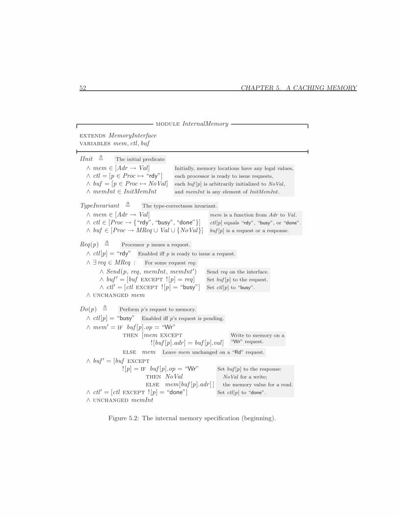
52 CHAPTER 5. A CACHING MEMORY
module InternalMemory
extends MemoryInterfacevariables mem, ctl , buf
IInit ∆= The initial predicate
∧ mem ∈ [Adr → Val ]∧ ctl = [p ∈ Proc 7→ “rdy”]∧ buf = [p ∈ Proc 7→ NoVal ]∧ memInt ∈ InitMemInt
Initially, memory locations have any legal values,
each processor is ready to issue requests,
each buf [p] is arbitrarily initialized to NoVal ,
and memInt is any element of InitMemInt .
TypeInvariant ∆= The type-correctness invariant.
∧ mem ∈ [Adr → Val ]∧ ctl ∈ [Proc → {“rdy”, “busy”, “done”}]∧ buf ∈ [Proc → MReq ∪ Val ∪ {NoVal}]
mem is a function from Adr to Val .
ctl [p] equals “rdy”, “busy”, or “done”.
buf [p] is a request or a response.
Req(p) ∆= Processor p issues a request.
∧ ctl [p] = “rdy” Enabled iff p is ready to issue a request.
∧ ∃ req ∈ MReq : For some request req :
∧ Send(p, req, memInt , memInt ′)∧ buf ′ = [buf except ! [p] = req]∧ ctl ′ = [ctl except ! [p] = “busy”]
Send req on the interface.
Set buf [p] to the request.
Set ctl [p] to “busy”.
∧ unchanged mem
Do(p) ∆= Perform p’s request to memory.
∧ ctl [p] = “busy” Enabled iff p’s request is pending.
∧ mem ′ = if buf [p].op = “Wr”then [mem except
! [buf [p].adr ] = buf [p].val ]else mem Leave mem unchanged on a “Rd” request.
Write to memory on a“Wr” request.
∧ buf ′ = [buf except! [p] = if buf [p].op = “Wr” Set buf [p] to the response:
NoVal for a write;
the memory value for a read.
Set ctl [p] to “done”.
then NoValelse mem[buf [p].adr ] ]
∧ ctl ′ = [ctl except ! [p] = “done”]∧ unchanged memInt
Figure 5.2: The internal memory specification (beginning).
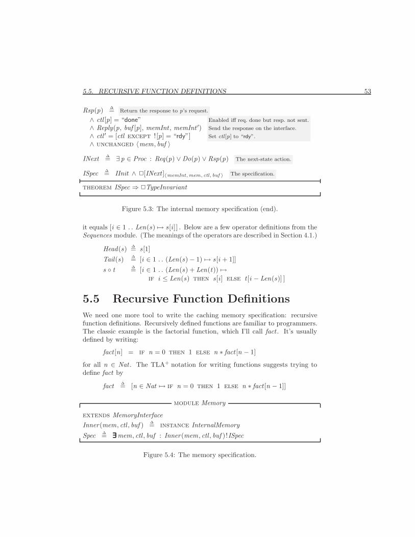
5.5. RECURSIVE FUNCTION DEFINITIONS 53
Rsp(p) ∆= Return the response to p’s request.
∧ ctl [p] = “done”∧ Reply(p, buf [p], memInt , memInt ′)∧ ctl ′ = [ctl except ! [p] = “rdy”]∧ unchanged 〈mem, buf 〉
Enabled iff req. done but resp. not sent.
Send the response on the interface.
Set ctl [p] to “rdy”.
INext ∆= ∃ p ∈ Proc : Req(p) ∨Do(p) ∨ Rsp(p) The next-state action.
ISpec ∆= IInit ∧ 2[INext ]〈memInt,mem, ctl, buf 〉 The specification.
theorem ISpec ⇒ 2TypeInvariant
Figure 5.3: The internal memory specification (end).
it equals [i ∈ 1 . . Len(s) 7→ s [i ]] . Below are a few operator definitions from theSequences module. (The meanings of the operators are described in Section 4.1.)
Head(s) ∆= s [1]
Tail(s) ∆= [i ∈ 1 . . (Len(s)− 1) 7→ s [i + 1]]
s ◦ t ∆= [i ∈ 1 . . (Len(s) + Len(t)) 7→if i ≤ Len(s) then s [i ] else t [i − Len(s)] ]
5.5 Recursive Function Definitions
We need one more tool to write the caching memory specification: recursivefunction definitions. Recursively defined functions are familiar to programmers.The classic example is the factorial function, which I’ll call fact . It’s usuallydefined by writing:
fact [n] = if n = 0 then 1 else n ∗ fact [n − 1]
for all n ∈ Nat . The TLA+ notation for writing functions suggests trying todefine fact by
fact ∆= [n ∈ Nat 7→ if n = 0 then 1 else n ∗ fact [n − 1]]
module Memory
extends MemoryInterfaceInner(mem, ctl , buf ) ∆= instance InternalMemory
Spec ∆= ∃∃∃∃∃∃mem, ctl , buf : Inner(mem, ctl , buf )!ISpec
Figure 5.4: The memory specification.
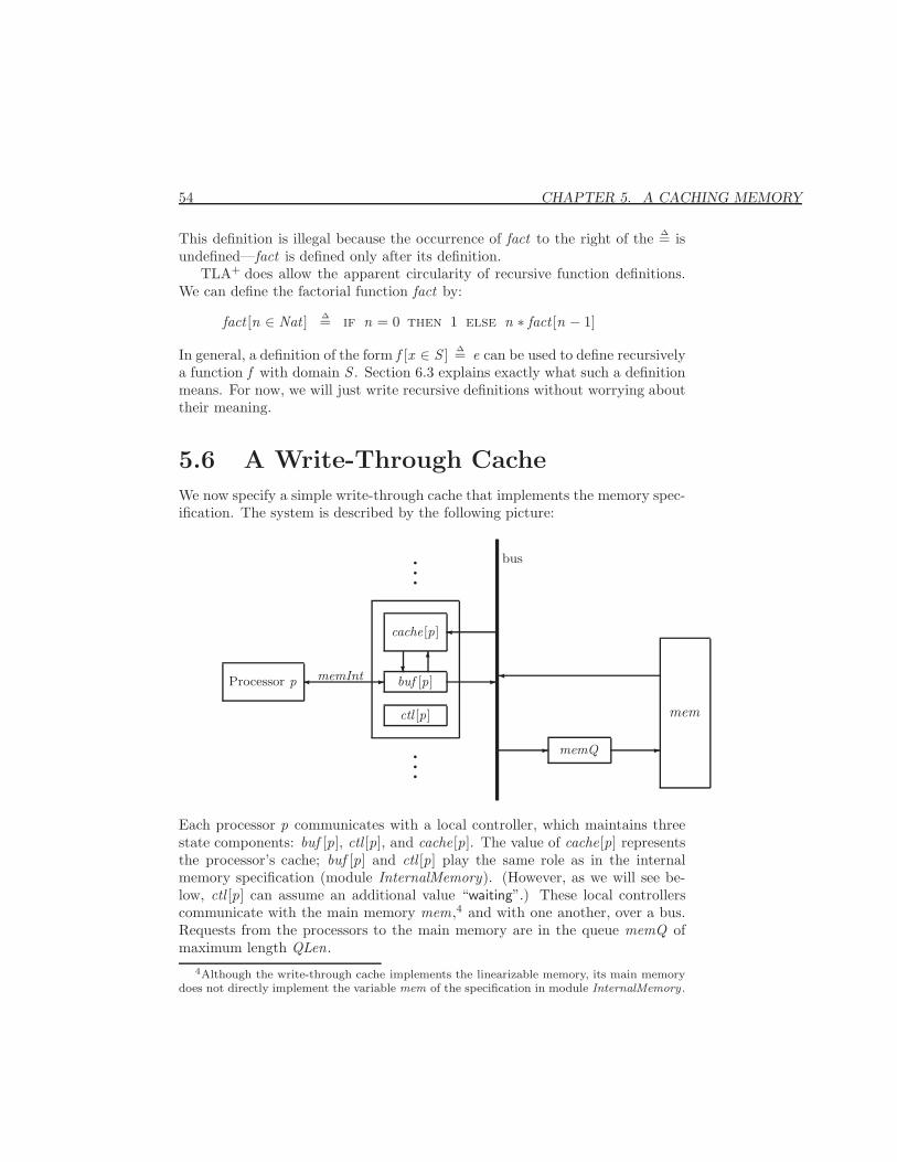
54 CHAPTER 5. A CACHING MEMORY
This definition is illegal because the occurrence of fact to the right of the ∆= isundefined—fact is defined only after its definition.
TLA+ does allow the apparent circularity of recursive function definitions.We can define the factorial function fact by:
fact [n ∈ Nat ] ∆= if n = 0 then 1 else n ∗ fact [n − 1]
In general, a definition of the form f [x ∈ S ] ∆= e can be used to define recursivelya function f with domain S . Section 6.3 explains exactly what such a definitionmeans. For now, we will just write recursive definitions without worrying abouttheir meaning.
5.6 A Write-Through Cache
We now specify a simple write-through cache that implements the memory spec-ification. The system is described by the following picture:
q
q
q
�cache[p]
6?buf [p]-�memInt -Processor p
ctl [p]
q
q
q
- -memQ
mem
�
bus
Each processor p communicates with a local controller, which maintains threestate components: buf [p], ctl [p], and cache[p]. The value of cache[p] representsthe processor’s cache; buf [p] and ctl [p] play the same role as in the internalmemory specification (module InternalMemory). (However, as we will see be-low, ctl [p] can assume an additional value “waiting”.) These local controllerscommunicate with the main memory mem,4 and with one another, over a bus.Requests from the processors to the main memory are in the queue memQ ofmaximum length QLen.
4Although the write-through cache implements the linearizable memory, its main memorydoes not directly implement the variable mem of the specification in module InternalMemory .
5.6. A WRITE-THROUGH CACHE 55
A write request by processor p is performed by the action DoWr(p). This isa write-through cache, meaning that every write request updates main memory.So, the DoWr(p) action writes the value into cache[p] and adds the write requestto the tail of memQ . It also updates cache[q] for any other processor q that hasa copy of the address in its cache. When the request reaches the head of memQ ,the action MemQWr stores the value in mem.
A read request by processor p is performed by the action DoRd(p), whichobtains the value from the cache. If the value is not in the cache, the actionRdMiss(p) adds the request to the tail of memQ and sets ctl [p] to “waiting”.When the enqueued request reaches the head of memQ , the action MemQRdreads the value and puts it in cache[p], enabling the DoRd(p) action.
We might expect the MemQRd action to read the value from mem. However,this could cause an error if there is a write to that address enqueued in memQbehind the read request. In that case, reading the value from memory couldlead to two processors having different values for the address in their caches:the one that issued the read request, and the one that issued the write requestthat followed the read in memQ . So, the MemQRd action must read the valuefrom the last write to that address in memQ , if there is such a write; otherwise,it reads the value from mem.
Eviction of an address from processor p’s cache is represented by a separateEvict(p) action. Since all cached values have been written to memory, evictiondoes nothing but remove the address from the cache. There is no reason to evictan address until the space is needed, so in an implementation, this action wouldbe executed only when a request for an uncached address is received from p andp’s cache is full. But that’s a performance optimization; it doesn’t affect thecorrectness of the algorithm, so it doesn’t appear in the specification. We allowa cached address to be evicted from p’s cache at any time—except if the addresswas just put there by a MemQRd action for the current request. This is thecase when ctl [p] equals “waiting” and buf [p].adr equals the cached address.
The actions Req(p) and Rsp(p), which represent processor p issuing a requestand the memory issuing a reply to p, are the same as the corresponding actionsof the memory specification, except that they also leave the new variables cacheand memQ unchanged.
To specify all these actions, we must decide how the processor caches andthe queue of requests to memory are represented by the variables memQ andcache. We let memQ be a sequence of pairs of the form 〈p, req 〉, where req isa request and p is the processor that issued it. For any memory address a, welet cache[p][a] be the value in p’s cache for address a (the “copy” of a in p’scache). If p’s cache does not have a copy of a, we let cache[p][a] equal NoVal .
The specification appears in module WriteThroughCache on pages 56–58.I’ll now go through this specification, explaining some of the finer points andsome notation that we haven’t encountered before.
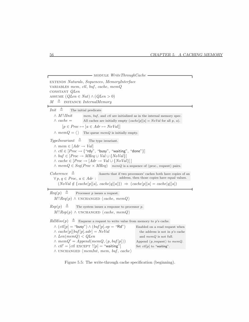
56 CHAPTER 5. A CACHING MEMORY
module WriteThroughCache
extends Naturals , Sequences , MemoryInterfacevariables mem, ctl , buf , cache, memQconstant QLenassume (QLen ∈ Nat) ∧ (QLen > 0)M ∆= instance InternalMemory
Init ∆= The initial predicate
∧ M !IInit∧ cache =
[p ∈ Proc 7→ [a ∈ Adr 7→ NoVal ]]∧ memQ = 〈 〉
mem, buf , and ctl are initialized as in the internal memory spec.
All caches are initially empty (cache[p][a] = NoVal for all p, a).
The queue memQ is initially empty.
TypeInvariant ∆= The type invariant.
∧ mem ∈ [Adr → Val ]∧ ctl ∈ [Proc → {“rdy”, “busy”, “waiting”, “done”}]∧ buf ∈ [Proc → MReq ∪ Val ∪ {NoVal}]∧ cache ∈ [Proc → [Adr → Val ∪ {NoVal}] ]∧ memQ ∈ Seq(Proc ×MReq) memQ is a sequence of 〈proc., request〉 pairs.
Coherence ∆= Asserts that if two processors’ caches both have copies of anaddress, then those copies have equal values.∀ p, q ∈ Proc, a ∈ Adr :
(NoVal /∈ {cache[p][a], cache[q][a]}) ⇒ (cache[p][a] = cache[q][a])
Req(p) ∆= Processor p issues a request.
M !Req(p) ∧ unchanged 〈cache, memQ 〉Rsp(p) ∆= The system issues a response to processor p.
M !Rsp(p) ∧ unchanged 〈cache, memQ 〉RdMiss(p) ∆= Enqueue a request to write value from memory to p’s cache.
∧ (ctl [p] = “busy”) ∧ (buf [p].op = “Rd”)∧ cache[p][buf [p].adr ] = NoVal∧ Len(memQ) < QLen∧ memQ ′ = Append(memQ , 〈p, buf [p]〉)∧ ctl ′ = [ctl except ! [p] = “waiting”]∧ unchanged 〈memInt , mem, buf , cache 〉
Enabled on a read request when
the address is not in p’s cache
and memQ is not full.
Append 〈p, request〉 to memQ .
Set ctl [p] to “waiting”.
Figure 5.5: The write-through cache specification (beginning).
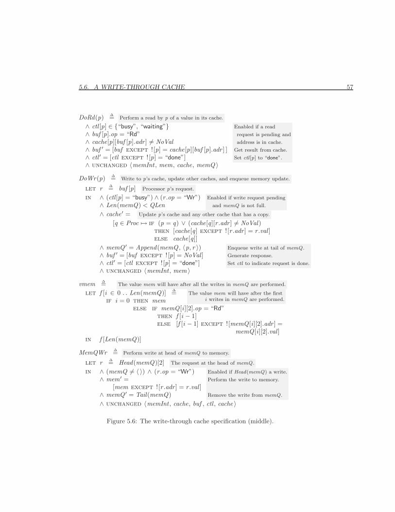
5.6. A WRITE-THROUGH CACHE 57
DoRd(p) ∆= Perform a read by p of a value in its cache.
∧ ctl [p] ∈ {“busy”, “waiting”}∧ buf [p].op = “Rd”∧ cache[p][buf [p].adr ] 6= NoVal∧ buf ′ = [buf except ! [p] = cache[p][buf [p].adr ] ]∧ ctl ′ = [ctl except ! [p] = “done”]∧ unchanged 〈memInt , mem, cache, memQ 〉
Enabled if a read
request is pending and
address is in cache.
Get result from cache.
Set ctl [p] to “done”.
DoWr(p) ∆= Write to p’s cache, update other caches, and enqueue memory update.
let r ∆= buf [p] Processor p’s request.
in ∧ (ctl [p] = “busy”) ∧ (r .op = “Wr”) Enabled if write request pending
and memQ is not full.∧ Len(memQ) < QLen∧ cache ′ = Update p’s cache and any other cache that has a copy.
[q ∈ Proc 7→ if (p = q) ∨ (cache[q][r .adr ] 6= NoVal)then [cache[q] except ! [r .adr ] = r .val ]else cache[q]]
∧ memQ ′ = Append(memQ , 〈p, r 〉) Enqueue write at tail of memQ .
Generate response.
Set ctl to indicate request is done.
∧ buf ′ = [buf except ! [p] = NoVal ]∧ ctl ′ = [ctl except ! [p] = “done”]∧ unchanged 〈memInt , mem 〉
vmem ∆= The value mem will have after all the writes in memQ are performed.
let f [i ∈ 0 . . Len(memQ)] ∆= The value mem will have after the firsti writes in memQ are performed.if i = 0 then mem
else if memQ [i ][2].op = “Rd”then f [i − 1]else [f [i − 1] except ! [memQ [i ][2].adr ] =
memQ [i ][2].val ]in f [Len(memQ)]
MemQWr ∆= Perform write at head of memQ to memory.
let r ∆= Head(memQ)[2] The request at the head of memQ .
in ∧ (memQ 6= 〈 〉) ∧ (r .op = “Wr”) Enabled if Head(memQ) a write.
Perform the write to memory.
Remove the write from memQ .
∧ mem ′ =[mem except ! [r .adr ] = r .val ]
∧ memQ ′ = Tail(memQ)∧ unchanged 〈memInt , cache, buf , ctl , cache 〉
Figure 5.6: The write-through cache specification (middle).
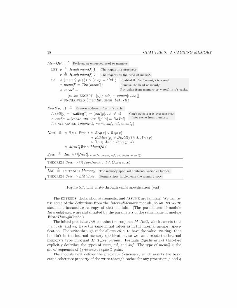
58 CHAPTER 5. A CACHING MEMORY
MemQRd ∆= Perform an enqueued read to memory.
let p ∆= Head(memQ)[1] The requesting processor.
r ∆= Head(memQ)[2] The request at the head of memQ .
in ∧ (memQ 6= 〈 〉) ∧ (r .op = “Rd”) Enabled if Head(memQ) is a read.
Remove the head of memQ .
Put value from memory or memQ in p’s cache.
∧ memQ ′ = Tail(memQ)∧ cache ′ =
[cache except ! [p][r .adr ] = vmem[r .adr ]]∧ unchanged 〈memInt , mem, buf , ctl 〉
Evict(p, a) ∆= Remove address a from p’s cache.
∧ (ctl [p] = “waiting”)⇒ (buf [p].adr 6= a) Can’t evict a if it was just readinto cache from memory.∧ cache ′ = [cache except ! [p][a] = NoVal ]
∧ unchanged 〈memInt , mem, buf , ctl , memQ 〉
Next ∆= ∨ ∃ p ∈ Proc : ∨ Req(p) ∨Rsp(p)∨ RdMiss(p) ∨DoRd(p) ∨DoWr(p)∨ ∃ a ∈ Adr : Evict(p, a)
∨ MemQWr ∨MemQRd
Spec ∆= Init ∧ 2[Next ]〈memInt,mem, buf , ctl, cache,memQ 〉
theorem Spec ⇒ 2(TypeInvariant ∧Coherence)
LM ∆= instance Memorytheorem Spec ⇒ LM !Spec
The memory spec. with internal variables hidden.
Formula Spec implements the memory spec.
Figure 5.7: The write-through cache specification (end).
The extends, declaration statements, and assume are familiar. We can re-use some of the definitions from the InternalMemory module, so an instancestatement instantiates a copy of that module. (The parameters of moduleInternalMemory are instantiated by the parameters of the same name in moduleWriteThroughCache.)
The initial predicate Init contains the conjunct M !IInit , which asserts thatmem, ctl , and buf have the same initial values as in the internal memory speci-fication. The write-through cache allows ctl [p] to have the value “waiting” thatit didn’t in the internal memory specification, so we can’t re-use the internalmemory’s type invariant M !TypeInvariant . Formula TypeInvariant thereforeexplicitly describes the types of mem, ctl , and buf . The type of memQ is theset of sequences of 〈processor, request〉 pairs.
The module next defines the predicate Coherence, which asserts the basiccache coherence property of the write-through cache: for any processors p and q
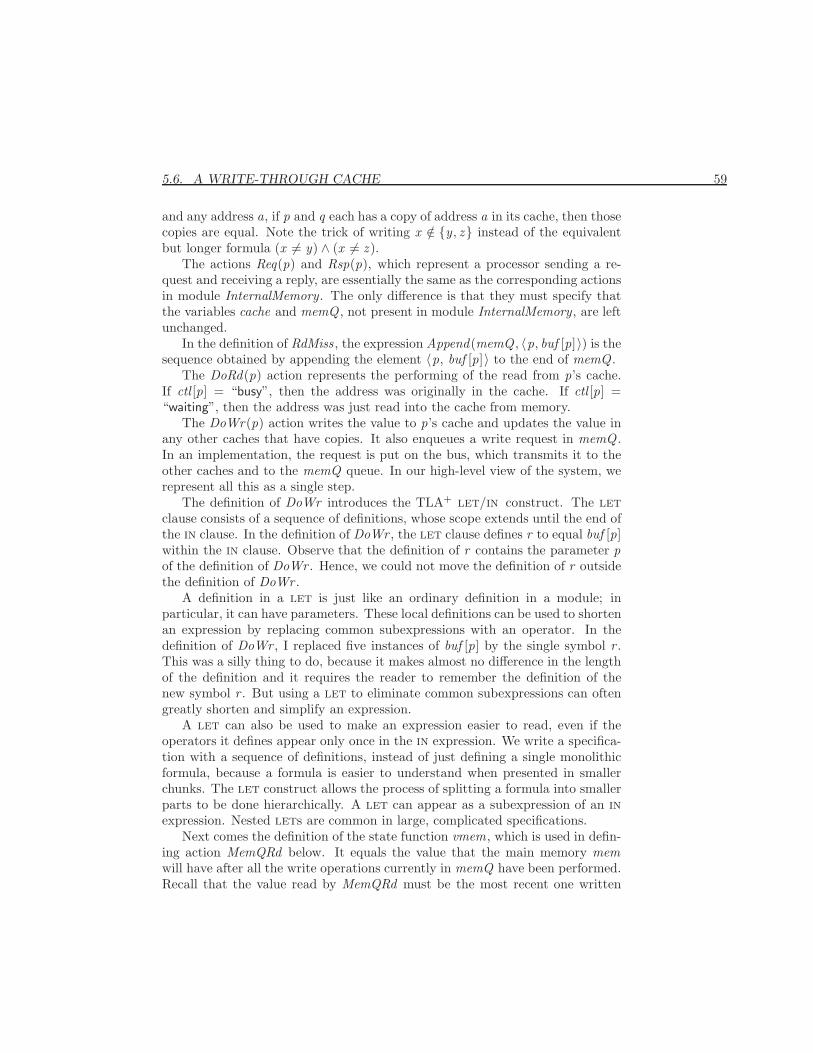
5.6. A WRITE-THROUGH CACHE 59
and any address a, if p and q each has a copy of address a in its cache, then thosecopies are equal. Note the trick of writing x /∈ {y, z} instead of the equivalentbut longer formula (x 6= y) ∧ (x 6= z ).
The actions Req(p) and Rsp(p), which represent a processor sending a re-quest and receiving a reply, are essentially the same as the corresponding actionsin module InternalMemory. The only difference is that they must specify thatthe variables cache and memQ , not present in module InternalMemory, are leftunchanged.
In the definition of RdMiss , the expression Append(memQ , 〈p, buf [p]〉) is thesequence obtained by appending the element 〈p, buf [p]〉 to the end of memQ .
The DoRd(p) action represents the performing of the read from p’s cache.If ctl [p] = “busy”, then the address was originally in the cache. If ctl [p] =“waiting”, then the address was just read into the cache from memory.
The DoWr(p) action writes the value to p’s cache and updates the value inany other caches that have copies. It also enqueues a write request in memQ .In an implementation, the request is put on the bus, which transmits it to theother caches and to the memQ queue. In our high-level view of the system, werepresent all this as a single step.
The definition of DoWr introduces the TLA+ let/in construct. The letclause consists of a sequence of definitions, whose scope extends until the end ofthe in clause. In the definition of DoWr , the let clause defines r to equal buf [p]within the in clause. Observe that the definition of r contains the parameter pof the definition of DoWr . Hence, we could not move the definition of r outsidethe definition of DoWr .
A definition in a let is just like an ordinary definition in a module; inparticular, it can have parameters. These local definitions can be used to shortenan expression by replacing common subexpressions with an operator. In thedefinition of DoWr , I replaced five instances of buf [p] by the single symbol r .This was a silly thing to do, because it makes almost no difference in the lengthof the definition and it requires the reader to remember the definition of thenew symbol r . But using a let to eliminate common subexpressions can oftengreatly shorten and simplify an expression.
A let can also be used to make an expression easier to read, even if theoperators it defines appear only once in the in expression. We write a specifica-tion with a sequence of definitions, instead of just defining a single monolithicformula, because a formula is easier to understand when presented in smallerchunks. The let construct allows the process of splitting a formula into smallerparts to be done hierarchically. A let can appear as a subexpression of an inexpression. Nested lets are common in large, complicated specifications.
Next comes the definition of the state function vmem, which is used in defin-ing action MemQRd below. It equals the value that the main memory memwill have after all the write operations currently in memQ have been performed.Recall that the value read by MemQRd must be the most recent one written
60 CHAPTER 5. A CACHING MEMORY
to that address—a value that may still be in memQ . That value is the onein vmem. The function vmem is defined in terms of the recursively definedfunction f , where f [i ] is the value mem will have after the first i operations inmemQ have been performed. Note that memQ [i ][2] is the second component(the request) of memQ [i ], the ith element in the sequence memQ .
The next two actions, MemQWr and MemQRd , represent the processing ofthe request at the head of the memQ queue—MemQWr for a write request,and MemQRd for a read request. These actions also use a let to make localdefinitions. Here, the definitions of p and r could be moved before the definitionof MemQWr . In fact, we could save space by replacing the two local definitions ofr with one global (within the module) definition. However, making the definitionof r global in this way would be somewhat distracting, since r is used only in thedefinitions of MemQWr and MemQRd . It might be better instead to combinethese two actions into one. Whether you put a definition into a let or makeit more global should depend on what makes the specification easier to read.Writing specifications is a craft whose mastery requires talent and hard work.
The Evict(p, a) action represents the operation of removing address a fromprocessor p’s cache. As explained above, we allow an address to be evicted atany time—unless the address was just written to satisfy a pending read request,which is the case iff ctl [p] = “waiting” and buf [p].adr = a. Note the use of the“double subscript” in the except expression of the action’s second conjunct.This conjunct “assigns NoVal to cache[p][a]”. If address a is not in p’s cache,then cache[p][a] already equals NoVal and an Evict(p, a) step is a stutteringstep.
The definitions of the next-state action Next and of the complete specifica-tion Spec are straightforward. The module closes with two theorems that arediscussed below.
5.7 Invariance
Module WriteThroughCache contains the theorem
theorem Spec ⇒ 2(TypeInvariant ∧Coherence)
which asserts that TypeInvariant ∧ Coherence is an invariant of Spec. A statepredicate P ∧ Q is always true iff both P and Q are always true, so 2(P ∧ Q)is equivalent to 2P ∧2Q . This implies that the theorem above is equivalent tothe two theorems:
theorem Spec ⇒ 2TypeInvarianttheorem Spec ⇒ 2Coherence
The first theorem is the usual type-invariance assertion. The second, whichasserts that Coherence is an invariant of Spec, expresses an important propertyof the algorithm.
5.7. INVARIANCE 61
Although TypeInvariant and Coherence are both invariants of the temporalformula Spec, they differ in a fundamental way. If s is any state satisfyingTypeInvariant , then any state t such that s → t is a Next step also satisfiesTypeInvariant . This property is expressed by:
theorem TypeInvariant ∧ Next ⇒ TypeInvariant ′
(Recall that TypeInvariant ′ is the formula obtained by priming all the variablesin formula TypeInvariant .) In general, when P ∧ N ⇒ P ′ holds, we say thatpredicate P is an invariant of action N . Predicate TypeInvariant is an invariant An invariant of
a specificationS that is alsoan invariant ofits next-state ac-tion is sometimescalled an inductiveinvariant of S .
of Spec because it is an invariant of Next and it is implied by the initial predicateInit .
Predicate Coherence is not an invariant of the next-state action Next . Forexample, suppose s is a state in which
• cache[p1][a] = 1
• cache[q][b] = NoVal , for all 〈q, b 〉 different from 〈p1, a 〉• mem[a] = 2
• memQ contains the single element 〈p2, [op 7→ “Rd”, adr 7→ a]〉for two different processors p1 and p2 and some address a. Such a state s (anassignment of values to variables) exists, assuming that there are at least twoprocessors and at least one address. Then Coherence is true in state s . Let tbe the state obtained from s by taking a MemQRd step. In state t , we havecache[p2][a] = 2 and cache[p1][a] = 1, so Coherence is false. Hence Coherenceis not an invariant of the next-state action.
Coherence is an invariant of formula Spec because states like s cannot occurin a behavior satisfying Spec. Proving its invariance is not so easy. We mustfind a predicate Inv that is an invariant of Next such that Inv implies Coherenceand is implied by the initial predicate Init .
Important properties of a specification can often be expressed as invariants.Proving that a state predicate P is an invariant of a specification means provinga formula of the form
Init ∧ 2[Next ]v ⇒ 2P
This is done by finding an appropriate state predicate Inv and proving
Init ⇒ Inv , Inv ∧ [Next ]v ⇒ Inv ′, Inv ⇒ P
Since our subject is specification, not proof, I won’t discuss how to find Inv .
62 CHAPTER 5. A CACHING MEMORY
5.8 Proving Implementation
Module WriteThroughCache ends with the theorem
theorem Spec ⇒ LM !Spec
where LM !Spec is formula Spec of module Memory. By definition of this formula(page 53), we can restate the theorem as
theorem Spec ⇒ ∃∃∃∃∃∃mem, ctl , buf : LM !Inner(mem, ctl , buf )!ISpec
where LM !Inner(mem, ctl , buf )!ISpec is formula ISpec of the InternalMemorymodule. The rules of logic tell us that to prove such a theorem, we must find“witnesses” for the quantified variables mem, ctl , and buf . These witness arestate functions (ordinary expressions with no primes), which I’ll call omem, octl ,and obuf , that satisfy:
Spec ⇒ LM !Inner(omem, octl , obuf )!ISpec(5.1)
The tuple 〈omem, octl , obuf 〉 of witness functions is called a refinement mapping,and we describe (5.1) as the assertion that Spec implements formula ISpec (ofmodule InternalMemory) under this refinement mapping. Intuitively, this meansSpec implies that the value of the tuple of state functions 〈memInt , omem, octl , obuf 〉changes the way ISpec asserts that the tuple of variables 〈memInt ,mem, ctl , buf 〉should change.
I will now briefly describe how we prove (5.1); for details, see [2]. Letme first introduce a bit of non-TLA+ notation. For any formula F of moduleInternalMemory, let F equal LM !Inner(omem, octl , obuf )!F , which is formulaF with omem, octl , and obuf substituted for mem, ctl , and buf . In particular,mem, ctl , and buf equal omem, octl , and obuf , respectively.
Replacing Spec and ISpec by their definitions transforms (5.1) to
Init ∧ 2[Next ]〈memInt,mem, buf , ctl, cache,memQ 〉⇒ IInit ∧ 2[INext ]〈memInt, mem, ctl, buf 〉
This is proved by finding an invariant Inv of Spec such that
∧ Init ⇒ IInit∧ Inv ∧ Next ⇒ ∨ INext
∨ unchanged 〈memInt , mem, ctl , buf 〉The second conjunct is called step simulation. It asserts that a Next step start-ing in a state satisfying the invariant Inv is either an INext step—a step thatchanges the 4-tuple 〈memInt , omem, octl , obuf 〉 the way an INext step changes〈memInt ,mem, ctl , buf 〉—or else it leaves that 4-tuple unchanged.
The mathematics of an implementation proof is simple, so the proof isstraightforward—in theory. For specifications of real systems, such proofs can
5.8. PROVING IMPLEMENTATION 63
be quite difficult. Going from the theory to practice requires turning the math-ematics of proofs into an engineering discipline—a subject that deserves a bookto itself. However, when writing specifications, it helps to understand refinementmappings and step simulation.
We now return to the question posed in Section 3.2: what is the relation be-tween the specifications of the asynchronous interface in modules AsynchInterfaceand Channel? Recall that module AsynchInterface describes the interface interms of the three variables val , rdy, and ack , while module Channel describesit with a single variable chan whose value is a record with val , rdy, and ackcomponents. In what sense are those two specifications of the interface equiva-lent?
One answer that now suggests itself is that each of the specifications shouldimplement the other under a refinement mapping. We expect formula Spec ofmodule Channel to imply the formula obtained from Spec of module AsynchInterfaceby substituting for its variables val , rdy, and ack the val , rdy, and ack com-ponents of the variable chan of module Channel . This assertion is expressedprecisely by the theorem in the following module.
module ChannelImplAsynch
extends ChannelAInt(val , rdy, ack) ∆= instance AsynchInterfacetheorem Spec ⇒ AInt(chan.val , chan.rdy, chan.ack)!Spec
Here, the refinement mapping substitutes 〈chan.val , chan.rdy, chan.ack 〉 forthe tuple 〈val , rdy, ack 〉 of variables in the formula Spec of module AsynchInterface.
Similarly, formula Spec of module AsynchInterface implies formula Spec ofmodule Channel with chan replaced by the record-valued expression:
[val 7→ val , rdy 7→ rdy, ack 7→ ack ]
(The first val in val 7→ val is the field name in the record constructor, while thesecond val is the variable of module AsynchInterface.)

64 CHAPTER 5. A CACHING MEMORY
Chapter 6
Some More Math
Our mathematics is built on a small, simple collection of concepts. You’vealready seen most of what’s needed to describe almost any kind of mathematics.All you lack are a handful of operators on sets that are described below inSection 6.1. After learning about them, you will be able to define all the datastructures and operations that occur in specifications.
While our mathematics is simple, its foundations are nonobvious—for exam-ple, the meanings of recursive function definitions and the choose operator aresubtle. This section discusses some of those foundations. Understanding themwill help you use mathematics more effectively.
6.1 Sets
The simple operations on sets described in Section 1.2 are all you’ll need forwriting most system specifications. However, you may occasionally have to usemore sophisticated operators—especially if you need to define data structuresbeyond tuples, records, and simple functions.
Two powerful operators of set theory are the unary operators union andsubset, defined as follows.
union S The union of the elements of S . In other words, a value e is an Mathematicianswrite union S as⋃
S .element of union S iff it is an element of an element of S . Forexample:
union {{1, 2}, {2, 3}, {3, 4}} = {1, 2, 3, 4}subset S The set of all subsets of S . In other words, T ∈ subset S iff Mathematicians
call unionS thepower set of Sand write it P(S)
or 2S .
T ⊆ S . For example:
subset {1, 2} = {{}, {1}, {2}, {1, 2}}
65
66 CHAPTER 6. SOME MORE MATH
Mathematicians often describe a set as “the set of all . . . such that . . . ”. TLA+
has two constructs that formalize such a description:
{x ∈ S : P} The subset of S consisting of all elements x satisfying propertyP . For example, the set of odd natural numbers can be written{n ∈ Nat : n % 2 = 1}. The identifier x is bound in P ; it may The modulus op-
erator % is de-scribed in Sec-tion 2.5.
not occur in S .
{e : x ∈ S} The set of elements of the form e, for all x in the set S . Forexample, {2 ∗ n + 1 : n ∈ Nat} is the set of all odd natural num-bers. The identifier x is bound in e; it may not occur in S .
The construct {e : x ∈ S} has the same generalizations as ∃ x ∈ S : F . For ex-ample, {e : x ∈ S , y ∈ T} is the set of all elements of the form e, for x in S andy in T . In the construct {x ∈ S : P}, we can let x be a tuple. For example,{〈y, z 〉 ∈ S : P} is the set of all pairs 〈y, z 〉 in the set S that satisfy P . TheBNF grammar of TLA+ in Section 14.1.2 specifies precisely what set expressionsyou can write.
All the set operators we’ve seen so far are built-in operators of TLA+. Thereis also a standard module FiniteSets that defines two operators:
Cardinality(S ) The number of elements in set S , if S is a finite set.
IsFiniteSet(S ) True iff S is a finite set.
Careless reasoning about sets can lead to problems. The classic example ofthis is Russell’s paradox:
Let R be the set of all sets S such that S /∈ S . The definition of Rimplies that R ∈ R is true iff R /∈ R is true.
The formula R /∈ R is simply the negation of R ∈ R, and a formula and itsnegation can neither both be true nor both be false. The source of the paradoxis that R isn’t a set. There’s no way to write it in TLA+. Intuitively, R is toobig to be a set. A collection C is too big to be a set if it is as big as the collectionof all sets—meaning that we can assign to every set a different element of C.That is, C is too big to be a set if we can define an operator SMap such that:
• SMap(S ) is in C, for any set S .
• If S and T are two different sets, then SMap(S ) 6= SMap(T ).
For example, the collection of all sequences of length 2 is too big to be a set; wecan define the operator SMap by
SMap(S ) ∆= 〈1,S 〉
6.2. SILLY EXPRESSIONS 67
6.2 Silly Expressions
Most modern programming languages introduce some form of type checking toprevent you from writing silly expressions like 3/“abc”. TLA+ is based on theusual formalization of mathematics, which doesn’t have types. In an untypedformalism, every syntactically well-formed expression has a meaning—even asilly expression like 3/“abc”. Mathematically, the expression 3/“abc” is nosillier than the expression 3/0, and mathematicians implicitly write that sillyexpression all the time. For example, consider the valid formula
∀ x ∈ Real : (x 6= 0)⇒ (x ∗ (3/x ) = 3)
where Real is the set of all real numbers. This asserts that (x 6= 0)⇒ (x ∗(3/x ) =3) is true for all real numbers x . Substituting 0 for x yields the valid formula(0 6= 0) ⇒ (0 ∗ (3/0) = 3) that contains the silly expression 3/0. It’s validbecause 0 6= 0 equals false, and false⇒ P is true for any formula P .
A correct formula can contain silly expressions. For example, 3/0 = 3/0 is acorrect formula because any value equals itself. However, the validity of a correctformula cannot depend on the meaning of a silly expression. If an expression issilly, then its meaning is probably unspecified. The definitions of 0, 3, /, and ∗(which are in the standard module Reals) don’t specify the value of 0 ∗ (3/0), sothere’s no way of knowing whether that value equals 3.
No sensible syntactic rules can prevent you from writing 3/0 without alsopreventing you from writing perfectly reasonable expressions. The typing rulesof programming languages introduce complexity and limitations on what you canwrite that don’t exist in ordinary mathematics. In a well-designed programminglanguage, the costs of types are balanced by benefits: types allow a compiler toproduce more efficient code, and type checking catches errors. For programminglanguages, the benefits seem to outweigh the costs. For writing specifications, Ihave found that the costs outweigh the benefits.
If you’re used to the constraints of programming languages, it may be a whilebefore you start taking advantage of the freedom afforded by mathematics. Atfirst, you won’t think of defining anything like the operator R defined on page 50of Section 5.2, which couldn’t be written in a typed programming language.
6.3 Recursive Function Definitions Revisited
Section 5.5 introduced recursive function definitions. Let’s now examine whatsuch definitions mean mathematically. Mathematicians usually define the fac-torial function fact by writing:
fact [n] = if n = 0 then 1 else n ∗ fact [n − 1], for all n ∈ Nat
68 CHAPTER 6. SOME MORE MATH
This definition can be justified by proving that it defines a unique function factwith domain Nat . In other words, fact is the unique value satisfying:
fact = [n ∈ Nat 7→ if n = 0 then 1 else n ∗ fact [n − 1]](6.1)
The choose operator, introduced on pages 47–48 of Section 5.1, allows us toexpress “the value satisfying property P” as choose x : P . We can thereforedefine fact as follows to be the value satisfying (6.1):
fact ∆= choose fact :fact = [n ∈ Nat 7→ if n = 0 then 1
else n ∗ fact [n − 1] ]
(6.2)
(Since the symbol fact is not yet defined in the expression to the right of the∆=, we can use it as the bound identifier in the choose expression.) The TLA+
definition
fact [n ∈ Nat ] ∆= if n = 0 then 1 else n ∗ fact [n − 1]
is simply an abbreviation for (6.2). In general, f [x ∈ S ] ∆= e is an abbreviationfor:
f ∆= choose f : f = [x ∈ S 7→ e](6.3)
TLA+ allows you to write silly definitions. For example, you can write
circ[n ∈ Nat ] ∆= choose y : y 6= circ[n](6.4)
This appears to define circ to be a function such that circ[n] 6= circ[n] forany natural number n. There obviously is no such function, so circ can’t bedefined to equal it. A recursive function definition doesn’t necessarily define afunction. If there is no f that equals [x ∈ S 7→ e], then (6.3) defines f to besome unspecified value. Thus, the nonsensical definition (6.4) defines circ to besome unknown value.
If we want to reason about a function f defined by f [x ∈ S ] ∆= e, we needto prove that there exists an f that equals [x ∈ S 7→ e]. The existence of f isobvious if f does not occur in e. If it does, so this is a recursive definition, thenthere is something to prove. Since I’m not discussing proofs, I won’t describehow to prove it. Intuitively, you have to check that, as in the case of the factorialfunction, the definition uniquely determines the value of f [x ] for every x in S .
Recursion is a common programming technique because programs must com-pute values using a small repertoire of simple elementary operations. It’s notused as often in mathematical definitions, where we needn’t worry about how tocompute the value and can use the powerful operators of logic and set theory.For example, the operators Head , Tail , and ◦ are defined in Section 5.4 with-out recursion, even though computer scientists usually define them recursively.Still, there are some things that are best defined inductively, using a recursivefunction definition.
6.4. FUNCTIONS VERSUS OPERATORS 69
6.4 Functions versus Operators
Consider these definitions, which we’ve seen before
Tail(s) ∆= [i ∈ 1 . . (Len(s) − 1) 7→ s [i + 1]]
fact [n ∈ Nat ] ∆= if n = 0 then 1 else n ∗ fact [n − 1]
They define two very different kinds of objects: fact is a function, and Tail isan operator. Functions and operators differ in a few basic ways.
Their most obvious difference is that a function like fact by itself is a completeexpression that denotes a value, but an operator like Tail is not. Both fact [n] ∈ Sand fact ∈ S are syntactically correct expressions. But, while Tail(n) ∈ S issyntactically correct, Tail ∈ S is not. It is gibberish—a meaningless string ofsymbols, like x+ = 0.
Their second difference is more profound. The definition of Tail definesTail(s) for all values of s . For example, it defines Tail(1/2) to equal
[i ∈ 1 . . (Len(1/2)− 1) 7→ (1/2)[i + 1]](6.5)
We have no idea what this expression means, because we don’t know whatLen(1/2) or (1/2)[i + 1] mean. But, whatever (6.5) means, it equals Tail(1/2).
The definition of fact defines fact [n] only for n ∈ Nat . It tells us noth-ing about the value of fact [1/2]. The expression fact [1/2] is syntactically well-formed, so it denotes some value. But the definition of fact tells us nothingabout what that value is.
Unlike an operator, a function must have a domain, which is a set. We cannotdefine a function Tail so that Tail [s ] is the tail of any nonempty sequence s ; thedomain of such a function would have to include all nonempty sequences, andthe collection of all such sequences is too big to be a set. (The operator SMapdefined by SMap(S ) ∆= 〈S 〉 maps every set to a different nonempty sequence.)Hence, we can’t define Tail to be a function.
Unlike a function, an operator cannot be defined recursively. However, wecan usually transform an illegal recursive operator definition into a nonrecursiveone using a recursive function definition. For example, let’s try to define theCardinality operator on the set of finite sets. (Recall that the cardinality of afinite set S is the number of elements in S .) The collection of all finite sets is toobig to be a set. (The operator SMap(S ) ∆= {S}maps every set S to a different set{S} of cardinality 1.) The Cardinality operator has a simple intuitive definition:
• Cardinality({}) = 0.
• If S is a nonempty finite set, then
Cardinality(S ) = 1 + Cardinality(S \ {x})where x is an arbitrary element of S . (The set S \ {x} contains all theelements of S except x .)
70 CHAPTER 6. SOME MORE MATH
Using the choose operator to describe an arbitrary element of S , we can writethis as the more formal-looking, but still illegal, definition:
Cardinality(S ) ∆=if S = {} then 0
else 1 + Cardinality(S \ {choose x : x ∈ S})This definition is illegal because it’s circular—only in a recursive function defi-nition can the symbol being defined appear to the right of the ∆= .
To turn this into a legal definition, observe that, for a given set S , we candefine a function CS such that CS [T ] equals the cardinality of T for every subsetT of S . The definition is
CS [T ∈ subset S ] ∆=if T = {} then 0
else 1 + CS [T \ {choose x : x ∈ T}]Since S is a subset of itself, this defines CS [S ] to equal Cardinality(S ), if S is afinite set. (We don’t know or care what CS [S ] equals if S is not finite.) So, wecan define the Cardinality operator by:
Cardinality(S ) ∆=let CS [T ∈ subset S ] ∆=
if T = {} then 0else 1 + CS [T \ {choose x : x ∈ T}]
in CS [S ]
Operators also differ from functions in that an operator can take an operatoras an argument. For example, we can define an operator IsPartialOrder so thatIsPartialOrder(R,S ) equals true iff the operator R defines an irreflexive partialorder on S . The definition is If you don’t know
what an irreflex-ive partial or-der is, read thisdefinition ofIsPartialOrderto find out.
IsPartialOrder(R( , ), S ) ∆=∧ ∀ x , y, z ∈ S : R(x , y) ∧ R(y, z )⇒ R(x , z )∧ ∀ x ∈ S : ¬R(x , x )
We could also use an infix-operator symbol like ≺ instead of R as the parameterof the definition, writing:
IsPartialOrder( ≺ , S ) ∆=∧ ∀ x , y, z ∈ S : (x ≺ y) ∧ (y ≺ z )⇒ (x ≺ z )∧ ∀ x ∈ S : ¬(x ≺ x )
The first argument of IsPartialOrder is an operator that takes two arguments;its second argument is an expression. Since > is an operator that takes two ar-guments, the expression IsPartialOrder(>,Nat) is syntactically correct. In fact,it’s valid—if > is defined to be the usual operator on numbers. The expression
6.5. USING FUNCTIONS 71
IsPartialOrder(+, 3) is also syntactically correct, but it’s silly and we have noidea whether or not it’s valid.
The last difference between operators and functions has nothing to do withmathematics and is an idiosyncrasy of TLA+: the language doesn’t permit youto define infix functions. So, if we want to define /, we have no choice but tomake it an operator.
One can write equally nonsensical things using functions or operators. How-ever, whether you use functions or operators may determine whether the non-sense you write is nonsyntactic gibberish or syntactically correct but semanti-cally silly. The string of symbols 2(“a”) is not a syntactically correct formulabecause 2 is not an operator. However, 2[“a”], which can also be written 2.a,is a syntactic correct expression. It’s nonsensical because 2 isn’t a function, sowe don’t know what 2[“a”] means. Similarly, Tail(s , t) is syntactically incorrectbecause Tail is an operator that takes a single argument. However, as explainedin Section 15.1.7 (page 275), fact [m,n] is syntactic sugar for fact [〈m,n 〉], so it isa syntactically correct, semantically silly formula. Whether an error is syntacticor semantic determines what kind of tool can catch it. In particular, the parserdescribed in Chapter 12 catches syntactic errors, but not semantic silliness.
The distinction between functions and operators seems to confuse some peo-ple. One reason is that, although this distinction exists in ordinary math, itusually goes unnoticed by mathematicians. If you point out to them that sub-set can’t be a function because its domain couldn’t be a set, mathematicianswill realize that they use operators like subset and ∈ all the time. But theynever think of them as forming a distinct kind of entity. Logicians will observethat the distinction between operators and values, including functions, arisesbecause TLA+ is a first-order logic rather than a higher-order logic.
When defining an object V , you may have to decide whether to make Van operator or a function. The differences between operators and functions willoften determine the decision. For example, if a variable may have V as its value,then V must be a function. Thus, in the memory specification of Section 5.3, wehad to represent the state of the memory by a function rather than an operator,since the variable mem couldn’t equal an operator. If these differences don’tdetermine whether to use an operator or a function, then it’s a matter of taste.I usually prefer operators.
6.5 Using Functions
Consider the following two formulas:
f ′ = [i ∈ Nat 7→ i + 1](6.6)
∀ i ∈ Nat : f ′[i ] = i + 1(6.7)
72 CHAPTER 6. SOME MORE MATH
These formulas both imply that f ′[i ] = i + 1 for every natural number i , butthey are not equivalent. Formula (6.6) uniquely determines f ′, asserting thatit’s a function with domain Nat . Formula (6.7) is satisfied by lots of differentvalues of f ′—for example, by the function
[i ∈ Real 7→ if i ∈ Nat then i + 1 else√
i ]
In fact, from (6.7), we can’t even deduce that f ′ is a function. Formula (6.6)implies formula (6.7), but not vice-versa.
When writing specifications, we almost always want to specify the new valueof a variable f rather than the new values of f [i ] for all i in some set. Wetherefore usually write (6.6) rather than (6.7),
6.6 Choose
The choose operator was introduced in the memory interface of Section 5.1 in The choose op-erator is knownto logicians asHilbert’s ε [3].
the simple idiom choose v : v /∈ S , which is an expression whose value is notan element of S . In Section 6.3 above, we saw that it is a powerful tool that canbe used in rather subtle ways.
The most common use for the choose operator is to “name” a uniquelyspecified value. For example, a/b is the unique real number that satisfies theformula a = b ∗ (a/b), if a and b are real numbers and b 6= 0. So, the standardmodule Reals defines division on the set Real of real numbers by
a/b ∆= choose c ∈ Real : a = b ∗ c
(The expression choose x ∈ S : P means choose x : (x ∈ S ) ∧ P .) If a is anonzero real number, then there is no real number c such that a = 0 ∗ c.Therefore, a/0 has an unspecified value. We don’t know what a real numbertimes a string equals, so we cannot say whether or not there is a real number csuch that a equals “xyz”. Hence, we don’t know what the value of a/“xyz” is.
People who do a lot of programming and not much mathematics often thinkthat choose must be a nondeterministic operator. In mathematics, there isno such thing as a nondeterministic operator or a nondeterministic function. Ifsome expression equals 42 today, then it will equal 42 tomorrow, and it will stillequal 42 a million years from tomorrow. The specification
(x = choose n : n ∈ Nat) ∧ 2[x ′ = choose n : n ∈ Nat ]x
allows only a single behavior—one in which x always equals choose n : n ∈ Nat ,which is some particular, unspecified natural number. It is very different fromthe specification
(x ∈ Nat) ∧ 2[x ′ ∈ Nat ]x
6.6. CHOOSE 73
that allows all behaviors in which x is always a natural number—possibly adifferent number in each state. This specification is highly nondeterministic,allowing lots of different behaviors.

74 CHAPTER 6. SOME MORE MATH

Chapter 7
Writing a Specification—SomeAdvice
You have now learned all you need to know about TLA+ to write your ownspecifications. Here are a few additional hints to help you get started.
7.1 Why to Specify
Specifications are written to help eliminate errors. Writing a specification re-quires effort; the benefits it provides must be worth that effort. There are severalbenefits:
• Writing a TLA+ specification can help the design process. Having to de-scribe a design precisely often reveals problems—subtle interactions and“corner cases” that are easily overlooked. These problems are easier to cor-rect when discovered in the design phase rather than after implementationhas begun.
• A TLA+ specification can provide a clear, concise way of communicatinga design. It helps ensure that the designers agree on what they havedesigned, and it provides a valuable guide to the engineers who implementand test the system. It may also help users understand the system.
• A TLA+ specification is a formal description to which tools can be appliedto help find errors in the design and to help in testing the system. Sometools for TLA+ specifications are being built.
Whether these benefits justify the effort of writing the specification depends onthe nature of the project. Specification is not an end in itself; it is just one ofmany tools that an engineer should be able to use when appropriate.
75
76 CHAPTER 7. WRITING A SPECIFICATION—SOME ADVICE
7.2 What to Specify
Although we talk about specifying a system, that’s not what we do. A specifi-cation is a mathematical model of a particular view of some part of a system.When writing a specification, the first thing you must choose is exactly whatpart of the system you want to describe. Sometimes the choice is obvious; oftenit isn’t. The cache-coherence protocol of a real multiprocessor computer may beintimately connected with how the processors execute instructions. Finding anabstraction that describes the coherence protocol while suppressing the detailsof instruction execution may be difficult. It may require defining an interfacebetween the processor and the memory that doesn’t exist in the actual systemdesign.
Remember that the purpose of a specification is to help avoid errors. Youshould specify those parts of the system for which a specification is most likelyto reveal errors. TLA+ is particularly effective at revealing concurrency errors—ones that arise through the interaction of asynchronous components. So, youshould concentrate your efforts on the parts of the system that are most likelyto have such errors.
7.3 The Grain of Atomicity
After choosing what part of the system to specify, you must choose the specifica-tion’s level of abstraction. The most important aspect of the level of abstractionis the grain of atomicity, the choice of what system changes are represented asa single step of a behavior. Sending a message in an actual system involvesmultiple suboperations, but we usually represent it as a single step. On theother hand, the sending of a message and its receipt are usually represented asseparate steps when specifying a distributed system.
The same sequence of system operations is represented by a shorter sequenceof steps in a coarser-grained representation than in a finer-grained one. Thisalmost always makes the coarser-grained specification simpler than the finer-grained one. However, the finer-grained specification more accurately describesthe behavior of the actual system. A coarser-grained specification may fail toreveal important details of the system.
There is no simple rule for deciding on the grain of atomicity. However, thereis one way of thinking about the granularity that can help. To describe it, weneed the TLA+ action-composition operator “·”. If A and B are actions, thenthe action A·B is executed by first executing A then B in a single step. Moreprecisely, A · B is the action defined by letting s → t be an A · B step iff thereexists a state u such that s → u is an A step and u → t is a B step.
When determining the grain of atomicity, we must decide whether to repre-sent the execution of an operation as a single step or as a sequence of steps, each
7.3. THE GRAIN OF ATOMICITY 77
corresponding to the execution of a suboperation. Let’s consider the simple caseof an operation consisting of two suboperations that are executed sequentially,where those suboperations are described by the two actions R and L. (Execut-ing R enables L and disables R.) When the operation’s execution is representedby two steps, each of those steps is an R step or an L step. The operation isthen described with the action R ∨ L. When its execution is represented bya single step, the operation is described with the action R·L.1 Let S2 be thefiner-grained specification in which the operation is executed in two steps, andlet S1 be the coarser-grained specification in which it is executed as a single R ·Lstep. To choose the grain of atomicity, we must choose whether to take S1 or S2as the specification. Let’s examine the relation between the two specifications.
We can transform any behavior σ satisfying S1 into a behavior σ satisfyingS2 by replacing each step s R·L→ t with the pair of steps s R→ u L→ t , for somestate u. If we regard σ as being equivalent to σ, then we can regard S1 as beinga strengthened version of S2—one that allows fewer behaviors. Specification S1requires that each R step be followed immediately by an L step, while S2 allowsbehaviors in which other steps come between the R and L steps. To choosethe appropriate grain of atomicity, we must decide whether those additionalbehaviors allowed by S2 are important.
The additional behaviors allowed by S2 are not important if the actual sys-tem executions they describe are also described by behaviors allowed by S1. So,we can ask whether each behavior τ satisfying S2 has a corresponding behaviorτ satisfying S1 that is, in some sense, equivalent to τ . One way to construct τfrom τ is to transform a sequence of steps
s R→ u1A1→ u2
A2→ u3 . . . unAn→ un+1
L→ t(7.1)
into the sequence
s A1→ v1 . . . vk−2Ak→ vk−1
R→ vkL→ vk+1
Ak+1→ vk+2 . . . vn+1An→ t(7.2)
where the Ai are other system actions that can be executed between the R andL steps. Both sequences start in state s and end in state t , but the intermediatestates may be different.
When is such a transformation possible? An answer can be given in terms ofcommutativity relations. We say that actions A and B commute if performingthem in either order produces the same result. Formally, A and B commute iffA · B is equivalent to B ·A. A simple sufficient condition for commutativity isthat two actions commute if (i) each one leaves unchanged any variable whosevalue may be changed by the other, and (ii) neither enables or disables the other.
1We actually describe the operation with an ordinary action, like the ones we’ve beenwriting, that is equivalent to R·L. The operator “·” rarely appears in an actual specification.If you’re ever tempted to use it, look for a better way to write the specification; you canprobably find one.
78 CHAPTER 7. WRITING A SPECIFICATION—SOME ADVICE
It’s not hard to see that we can transform (7.1) to (7.2) in the following twocases:
• R commutes with each Ai . (In this case, k = n.)
• L commutes with each Ai . (In this case, k = 0.)
In general, if an operation consists of a sequence of m subactions, we must decidewhether to choose the finer-grained representation O1 ∨ O2 ∨ . . . ∨ Om or thecoarser-grained one O1 · O2 · · ·Om . The generalization of the transformationfrom (7.1) to (7.2) is one that transforms an arbitrary behavior satisfying thefiner-grained specification into one in which the sequence of O1, O2, . . . , Om
steps come one right after the other. Such a transformation is possible if all butone of the actions O i commute with every other system action. Commutativitycan be replaced by weaker conditions, but it is the most common case.
By commuting actions and replacing a sequence s O1→ · · · Om→ t of steps bya single O1 · · ·Om step, you may be able to transform any behavior of a finer-grained specification into a corresponding behavior of a coarser-grained one.But that doesn’t mean that the coarser-grained specification is just as good asthe finer-grained one. The sequences (7.1) and (7.2) are not the same, and asequence of O i steps is not the same as a single O1 · · ·Om step. Whether youcan consider the transformed behavior to be equivalent to the original one, anduse the coarser-grained specification, depends on the particular system you arespecifying and on the purpose of the specification. Understanding the relationbetween finer- and coarser-grained specifications can help you choose betweenthem; it won’t make the choice for you.
7.4 The Data Structures
Another aspect of a specification’s level of abstraction is the accuracy with whichit describes the system’s data structures. For example, should the specificationof a programming interface describe the actual layout of a procedure’s argumentsin memory, or should the arguments be represented more abstractly?
To answer such a question, you must remember that the purpose of the spec-ification is to help catch errors. A precise description of the layout of procedurearguments will help prevent errors caused by misunderstandings about that lay-out, but at the cost of complicating the programming interface’s specification.The cost is justified only if such errors are likely to be a real problem and theTLA+ specification provides the best way to avoid them.
If the purpose of the specification is to catch errors caused by the asyn-chronous interaction of concurrently executing components, then detailed de-scriptions of data structures will be a needless complication. So, you will proba-bly want to use high-level, abstract descriptions of the system’s data structures
7.5. WRITING THE SPECIFICATION 79
in the specification. For example, to specify a program interface, you mightintroduce constant parameters to represent the actions of calling and return-ing from a procedure—parameters analogous to Send and Reply of the memoryinterface described in Section 5.1 (page 45).
7.5 Writing the Specification
Once you’ve chosen the part of the system to specify and the level of abstraction,you’re ready to start writing the TLA+ specification. We’ve already seen howthis is done; let’s review the steps.
First, pick the variables and define the type invariant and initial predicate.In the course of doing this, you will determine the constant parameters andassumptions about them that you need. You may also have to define someadditional constants.
Next, write the next-state action, which forms the bulk of the specification.Sketching a few sample behaviors may help you get started. You must first decidehow to decompose the next-state action as the disjunction of actions describingthe different kinds of system operations. You then define those actions. The goalis to make the action definitions as compact and easy to read as possible. Thisrequires carefully structuring them. One way to reduce the size of a specificationis to define state predicates and state functions that are used in several differentaction definitions. When writing the action definitions, you will determine whichof the standard modules you will need to use and add the appropriate extendsstatement. You may also have to define some constant operators for the datastructures that you are using.
You must now write the temporal part of the specification. (If you wantto specify liveness properties, you have to choose the fairness conditions, asdescribed below in Chapter . You then combine the initial predicate, next-stateaction, and any fairness conditions you’ve chosen into the definition of a singletemporal formula that is the specification.
Finally, you can assert theorems about the specification. If nothing else, youmay want to add a type-correctness theorem.
7.6 Some Further Hints
Here are a few miscellaneous suggestions that may help you write better speci-fications.
80 CHAPTER 7. WRITING A SPECIFICATION—SOME ADVICE
Don’t be too clever.
Cleverness can make a specification hard to read—and even wrong. The formulaq = 〈h′ 〉 ◦ q ′ may look like a nice, short way of writing:
(h′ = Head(q)) ∧ (q ′ = Tail(q))(7.3)
But not only is q = 〈h′ 〉 ◦ q ′ harder to understand than (7.3), it’s also wrong.We don’t know what a ◦ b equals if a and b are not both sequences, so we don’tknow whether h′ = Head(q) and q ′ = Tail(q) are the only values of h′ and q ′
that satisfy q = 〈h′ 〉 ◦ q ′. There could be other values of h′ and q ′, which arenot sequences, that satisfy the formula.
A type invariant is not an assumption.
Type invariance is a property of a specification, not an assumption. Whenwriting a specification, we usually define a type invariant. But that’s just adefinition; a definition is not an assumption. Suppose you define a type invariantthat asserts that a variable n is of type Nat . You may be tempted to then thinkthat a conjunct n ′ > 7 in an action asserts that n ′ is a natural number greaterthan 7. It doesn’t. The formula n ′ > 7 asserts only that n ′ > 7. It is satisfiedif n ′ =
√96 as well as if n ′ = 8. Since we don’t know whether or not “abc” > 7
is true, it might be satisfied if n ′ = “abc”. The meaning of the formula is notchanged just because you’ve defined a type invariant that asserts n ∈ Nat .
In general, you may want to describe the new value of a variable x by assert-ing some property of x ′. However, the next-state relation should imply that x ′
is an element of some suitable set. For example, a specification might define:2
Action1 ∆= (n ′ > 7) ∧ . . .
Action2 ∆= (n ′ ≤ 6) ∧ . . .
Next ∆= (n ′ ∈ Nat) ∧ (Action1 ∨ Action2)
Don’t be too abstract
Suppose a user interacts with the system by typing on a keyboard. We coulddescribe the interaction abstractly with a variable typ and an operator parameterKeyStroke, where the action KeyStroke(“a”, typ, typ′) represents the user typingan “a”. This is the approach we took in describing the communication betweenthe processors and the memory in the MemoryInterface module (page 48).
A more concrete description would be to let kbd represent the state of thekeyboard, perhaps letting kbd = {} mean that no key is depressed, and kbd ={“a”} mean that the a key is depressed. The typing of an a is represented by
2An alternative approach is to define Next to equal Action1 ∨ Action2 and to let thespecification be Init ∧ 2[Next ]... ∧ 2(n ∈ Nat). But it’s usually better to stick to the simpleform Init ∧ 2[Next ]... for specifications.
7.6. SOME FURTHER HINTS 81
two steps, a [kbd = {}] → [kbd = {“a”}] step represents the pressing of the akey, and a [kbd = {“a”}] → [kbd = {}] step represents its release. This is theapproach we took in the asynchronous interface specifications of Chapter 3.
The abstract interface is simpler; typing an a is represented by a singleKeyStroke(“a”, typ, typ′) step instead of a pair of steps. However, using theconcrete representation leads us naturally to ask: what if the user presses the akey and, before releasing it, presses the b key? That’s easy to describe with theconcrete representation. The state with both keys depressed is kbd = {a, b}.Pressing and releasing a key are represented simply by the two actions
Press(k) ∆= kbd ′ = kbd ∪ {“k”} Release(k) ∆= kbd ′ = kbd \ {“k”}This possibility cannot be expressed with the simple abstract interface. Toexpress it abstractly, we would have to replace the parameter KeyStroke withtwo parameters Press and Release, and we would have to express explicitly theproperty that a key can’t be released until it has been depressed, and vice-versa.The more concrete representation is simpler.
We might decide that we don’t want to consider the possibility of the userpressing two keys at once, and that we prefer the abstract representation. Butthat should be a conscious decision. Our abstraction should not blind us to whatcan happen in the actual system. When in doubt, it’s safer to use a concreterepresentation that more accurately describes the real system. That way, youare less likely to overlook problems that can arise in the actual system.
Don’t assume values that look different are unequal.
The rules of TLA+ do not imply that 1 6= “a”. If the system can send a messagethat is either a string or a number, represent the message as a record with atype and value field—for example,
[type 7→ “String”, value 7→ “a”] or [type 7→ “Nat”, value 7→ 1]
We know that these two values are different because they have different typefields.
Move quantification to the outside.
Specifications are usually easier to read if ∃ is moved outside disjunctions and∀ is moved outside conjunctions. For example, instead of:
Up ∆= ∃ e ∈ Elevator : . . .
Down ∆= ∃ e ∈ Elevator : . . .
Move ∆= Up ∨ Down
82 CHAPTER 7. WRITING A SPECIFICATION—SOME ADVICE
it’s usually better to write:
Up(e) ∆= . . .
Down(e) ∆= . . .
Move ∆= ∃ e ∈ Elevator : Up(e) ∨ Down(e)
Prime only what you mean to prime.
When writing an action, be careful where you put your primes. The expressionf [e]′ equals f ′[e ′]; it equals f ′[e] only if e ′ = e, which need not be true if theexpression e contains variables. Be especially careful when priming an operatorwhose definition contains a variable. For example, suppose x is a variable andop is defined by
op(a) ∆= x + a
Then op(y)′ equals (x+y)′, which equals x ′+y ′, while op(y ′) equals x+y ′. Thereis no way to use op and ′ to write the formula x ′ + y. (Writing op′(y) doesn’twork because it’s illegal—you can only prime an expression, not an operator.)
Write comments as comments.
Don’t put comments into the specification itself. I have seen people write thingslike the following action definition:
A ∆= ∨ ∧ x ≥ 0∧ . . .∨ ∧ x < 0∧ false
The second disjunct is meant to indicate that the writer intended A not to beenabled when x < 0. But that disjunct is completely redundant, since F ∧falseequals false, and F ∨false equals F , for any formula F . So the second disjunctof the definition serves only as a form of comment. It’s better to write:
A ∆= ∧ x ≥ 0∧ . . .
A is not enabled if x < 0
7.7 When and How to Specify
Specifications are often written later than they should be. Engineers are usuallyunder severe time constraints, and they may feel that writing a specification willslow them down. Only after a design has become so complex that they needhelp understanding it do engineers think about writing a precise specification.
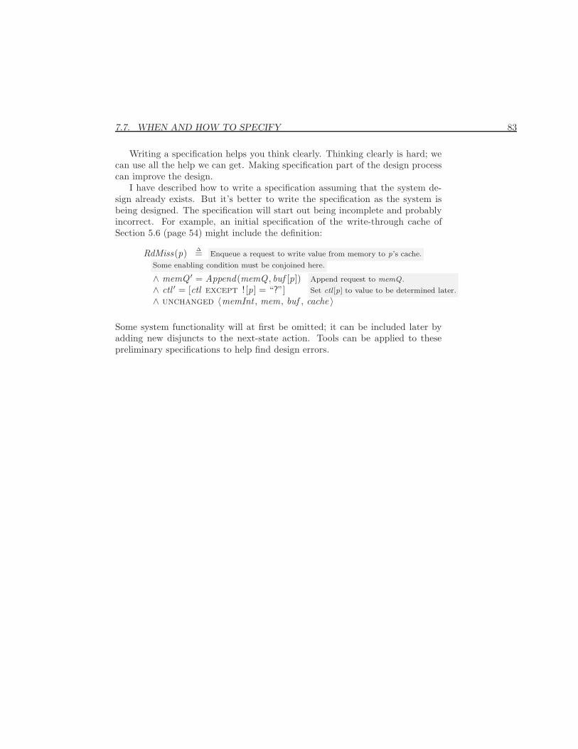
7.7. WHEN AND HOW TO SPECIFY 83
Writing a specification helps you think clearly. Thinking clearly is hard; wecan use all the help we can get. Making specification part of the design processcan improve the design.
I have described how to write a specification assuming that the system de-sign already exists. But it’s better to write the specification as the system isbeing designed. The specification will start out being incomplete and probablyincorrect. For example, an initial specification of the write-through cache ofSection 5.6 (page 54) might include the definition:
RdMiss(p) ∆= Enqueue a request to write value from memory to p’s cache.
Some enabling condition must be conjoined here.
∧ memQ ′ = Append(memQ , buf [p])∧ ctl ′ = [ctl except ! [p] = “?”]∧ unchanged 〈memInt , mem, buf , cache 〉
Append request to memQ .
Set ctl [p] to value to be determined later.
Some system functionality will at first be omitted; it can be included later byadding new disjuncts to the next-state action. Tools can be applied to thesepreliminary specifications to help find design errors.

84 CHAPTER 7. WRITING A SPECIFICATION—SOME ADVICE

Part II
More Advanced Topics
85

Chapter 8
Liveness and Fairness
The specifications we have written so far say what a system must not do. Theclock must not advance from 11 to 9; the receiver must not receive a message ifthe FIFO is empty. They don’t require that the system ever do anything. Theclock need never tick; the sender need never send any messages. Our specifi-cations have described what are called safety properties. If a safety property isviolated, it is violated at some particular point in the behavior—by a step thatadvances the clock from 11 to 9, or that reads the wrong value from memory.Therefore, we can talk about a safety property being satisfied by a finite behav-ior, which means that it has not been violated by any step so far. (Formally,it means that the behavior obtained by adding infinitely many stuttering stepssatisfies the property.)
We now learn how to specify that something does happen: the clock keepsticking; a value is eventually read from memory. We specify liveness properties,which cannot be violated at any particular instant. Only by examining an entireinfinite behavior can we tell that the clock has stopped ticking, or that a messageis never sent.
8.1 Temporal Formulas
To specify liveness properties we must learn to express them as temporal formu-las. We now take a more rigorous look at what a temporal formula means.
Recall that a state assigns a value to every variable, and a behavior is aninfinite sequence of states. A temporal formula is true or false of a behavior. Letσ |= F be the truth value of the formula F for the behavior σ, so σ satisfies Fiff σ |= F equals true. To define the meaning of a temporal formula F , we haveto explain how to determine the value of σ |= F for any behavior σ. For now,we consider only temporal formulas that don’t contain the temporal existential
87
88 CHAPTER 8. LIVENESS AND FAIRNESS
quantifier ∃∃∃∃∃∃ .It’s easy to define the meaning of a Boolean combination of temporal formulas
in terms of the meanings of those formulas. The formula F ∧ G is true of abehavior σ iff both F and G are true of σ, and ¬F is true of σ iff F is false forσ:
σ |= (F ∧G) ∆= (σ |= F ) ∧ (σ |= G) σ |= ¬F ∆= ¬ (σ |= F )
This defines the meanings of ∧ and ¬ as operators on temporal formulas. Themeanings of the other Boolean operators are similarly defined. In the same way,we can define the ordinary predicate-logic quantifiers ∀ and ∃ as operators ontemporal formulas—for example:
σ |= (∃ r : F ) ∆= ∃ r : (σ |= F )
We will discuss quantifiers in Section 8.6. For now, we ignore quantification intemporal formulas.
All the temporal formulas not containing ∃∃∃∃∃∃ that we’ve seen have been Bool-ean combinations of the following three simple kinds of formulas. (Recall thedefinitions of state function and state predicate on page 25 in Section 3.1.)
• A state predicate. It is interpreted as a temporal formula that is true of abehavior iff it is true in the first state of the behavior.
• A formula 2P , where P is a state predicate. It is true of a behavior iff Pis true in every state of the behavior.
• A formula 2[N ]v , where N is an action and v is a state function. It is trueof a behavior iff every successive pair of steps in the behavior is a [N ]vstep.
Since a state predicate is an action that contains no primed variables, we canboth combine and generalize these three kinds of temporal formulas into the twokinds of formulas A and 2A, where A is an action.
Generalizing from state functions, we interpret an arbitrary action A as atemporal formula by defining σ |= A to be true iff the first two states of σ arean A step. For any behavior σ, let σ0, σ1, . . . be the sequence of states thatmake up σ. Then the meaning of an action A as a temporal formula is definedby letting σ |= A be true iff the pair 〈σ0, σ1 〉 of states is an A step. We defineσ |= 2A to be true iff, for all n ∈ Nat , the pair 〈σn , σn+1 〉 of states is an A step.We now generalize this to the definition of σ |= 2F for an arbitrary temporalformula F .
For any behavior σ and natural number n, let σ+n be the suffix of σ obtainedby deleting its first n states:
σ+n ∆= σn , σn+1, σn+2, . . .
8.1. TEMPORAL FORMULAS 89
The successive pair of states 〈σn , σn+1 〉 of σ is the first pair of states of σ+n ,and 〈σn , σn+1 〉 is an A step iff σ+n satisfies A. In other words:
(σ |= 2A) ≡ ∀n ∈ Nat : σ+n |= A
So, we can generalize the definition of σ |= 2A to
σ |= 2F ∆= ∀n ∈ Nat : σ+n |= F
for any temporal formula F . In other words, σ satisfies 2F iff every suffix σ+n
of σ satisfies F . This defines the temporal operator 2.We have now defined the meaning of any temporal formula built from ac-
tions (including state predicates), Boolean operators, and the 2 operator. Forexample:
σ |= 2((x = 1)⇒ 2(y > 0))≡ ∀n ∈ Nat : σ+n |= ((x = 1)⇒ 2(y > 0)) By the meaning of 2.
≡ ∀n ∈ Nat : (σ+n |= (x = 1))⇒ (σ+n |= 2(y > 0)) By the meaning of ⇒.
≡ ∀n ∈ Nat : (σ+n |= (x = 1))⇒(∀m ∈ Nat : (σ+n)+m |= (y > 0))
By the meaning of 2.
Thus, σ |= 2((x = 1)⇒ 2(y > 0)) is true iff, for all n ∈ Nat , if x = 1 is true instate σn , then y > 0 is true in all states σn+m with m ≥ 0.
We saw in Section 2.2 that a specification should allow stuttering steps—onesthat leave unchanged all the variables appearing in the formula. A stutteringstep represents a change only to some part of the system not described by theformula; adding it to the behavior should not affect the truth of the formula. Wesay that a formula F is invariant under stuttering1 if adding a stuttering step toa behavior σ does not affect whether F is true of σ. (This implies that removinga stuttering step from σ also does not affect the truth of σ |= F .) A sensibleformula should be invariant under stuttering. There’s no point writing formulasthat aren’t sensible, so TLA+ allows you to write only temporal formulas thatare invariant under stuttering.
An arbitrary action, viewed as a temporal formula, is not invariant understuttering. The action x ′ = x +1 is true for a behavior in which x is incrementedby 1 in the first step; adding an initial stuttering step makes it false. A statepredicate is invariant under stuttering, since its truth depends only on the firststate of a behavior, and adding a stuttering step doesn’t change the first state.The formula 2[N ]v is also invariant under stuttering, for any action N and statefunction v . It’s not hard to see that invariance under stuttering is preserved by 2
and by the Boolean operators. So, state predicates, formulas of the form 2[N ]v ,and all formulas obtainable from them by applying 2 and Boolean operators
1This is a completely new sense of the word invariant ; it has nothing to do with the conceptof invariance discussed already.
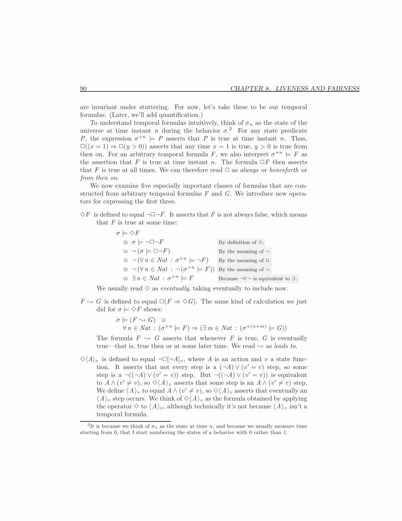
90 CHAPTER 8. LIVENESS AND FAIRNESS
are invariant under stuttering. For now, let’s take these to be our temporalformulas. (Later, we’ll add quantification.)
To understand temporal formulas intuitively, think of σn as the state of theuniverse at time instant n during the behavior σ.2 For any state predicateP , the expression σ+n |= P asserts that P is true at time instant n. Thus,2((x = 1)⇒ 2(y > 0)) asserts that any time x = 1 is true, y > 0 is true fromthen on. For an arbitrary temporal formula F , we also interpret σ+n |= F asthe assertion that F is true at time instant n. The formula 2F then assertsthat F is true at all times. We can therefore read 2 as always or henceforth orfrom then on.
We now examine five especially important classes of formulas that are con-structed from arbitrary temporal formulas F and G. We introduce new opera-tors for expressing the first three.
3F is defined to equal ¬2¬F . It asserts that F is not always false, which meansthat F is true at some time:
σ |= 3F≡ σ |= ¬2¬F By definition of 3.
≡ ¬ (σ |= 2¬F ) By the meaning of ¬.
≡ ¬ (∀n ∈ Nat : σ+n |= ¬F ) By the meaning of 2.
≡ ¬ (∀n ∈ Nat : ¬ (σ+n |= F )) By the meaning of ¬.
≡ ∃n ∈ Nat : σ+n |= F Because ¬∀¬ is equivalent to ∃ .
We usually read 3 as eventually, taking eventually to include now.
F ; G is defined to equal 2(F ⇒ 3G). The same kind of calculation we justdid for σ |= 3F shows:
σ |= (F ; G) ≡∀n ∈ Nat : (σ+n |= F )⇒ (∃m ∈ Nat : (σ+(n+m) |= G))
The formula F ; G asserts that whenever F is true, G is eventuallytrue—that is, true then or at some later time. We read ; as leads to.
3〈A〉v is defined to equal ¬2[¬A]v , where A is an action and v a state func-tion. It asserts that not every step is a (¬A) ∨ (v ′ = v) step, so somestep is a ¬((¬A) ∨ (v ′ = v)) step. But ¬((¬A) ∨ (v ′ = v)) is equivalentto A ∧ (v ′ 6= v), so 3〈A〉v asserts that some step is an A ∧ (v ′ 6= v) step.We define 〈A〉v to equal A ∧ (v ′ 6= v), so 3〈A〉v asserts that eventually an〈A〉v step occurs. We think of 3〈A〉v as the formula obtained by applyingthe operator 3 to 〈A〉v , although technically it’s not because 〈A〉v isn’t atemporal formula.
2It is because we think of σn as the state at time n, and because we usually measure timestarting from 0, that I start numbering the states of a behavior with 0 rather than 1.
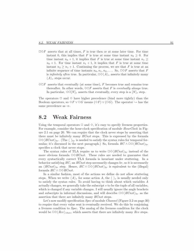
8.2. WEAK FAIRNESS 91
23F asserts that at all times, F is true then or at some later time. For timeinstant 0, this implies that F is true at some time instant n0 ≥ 0. Fortime instant n0 + 1, it implies that F is true at some time instant n1 ≥n0 + 1. For time instant n1 + 1, it implies that F is true at some timeinstant n2 ≥ n1 + 1. Continuing the process, we see that F is true at aninfinite sequence of time instants n0,n1,n2, . . . . So, 23F asserts that Fis infinitely often true. In particular, 23〈A〉v asserts that infinitely many〈A〉v steps occur.
32F asserts that eventually (at some time), F becomes true and remains truethereafter. In other words, 32F asserts that F is eventually always true.In particular, 32[N ]v asserts that eventually, every step is a [N ]v step.
The operators 2 and 3 have higher precedence (bind more tightly) than theBoolean operators, so 3F ∨ 2G means (3F ) ∨ (2G). The operator ; has thesame precedence as ⇒.
8.2 Weak Fairness
Using the temporal operators 2 and 3, it’s easy to specify liveness properties.For example, consider the hour-clock specification of module HourClock in Fig-ure 2.1 on page 20. We can require that the clock never stops by asserting thatthere must be infinitely many HCnxt steps. This is expressed by the formula23〈HCnxt 〉hr . (The 〈 〉hr is needed to satisfy the syntax rules for temporal for-mulas; it’s discussed in the next paragraph.) So, formula HC ∧23〈HCnxt 〉hrspecifies a clock that never stops.
The syntax rules of TLA require us to write 23〈HCnxt 〉hr instead of themore obvious formula 23HCnxt . These rules are needed to guarantee thatevery syntactically correct TLA formula is invariant under stuttering. In abehavior satisfying HC , an HCnxt step necessarily changes hr , so it is necessarilyan 〈HCnxt 〉hr step. Hence, HC ∧ 23〈HCnxt 〉hr is equivalent to the (illegal)formula HC ∧ 23HCnxt .
In a similar fashion, most of the actions we define do not allow stutteringsteps. When we write 〈A〉v for some action A, the 〈 〉v is usually needed onlyto satisfy the syntax rules. To avoid having to think about which variables Aactually changes, we generally take the subscript v to be the tuple of all variables,which is changed if any variable changes. I will usually ignore the angle bracketsand subscripts in informal discussions, and will describe 23〈HCnxt 〉hr as theassertion that there are infinitely many HCnxt steps.
Let’s now modify specification Spec of module Channel (Figure 3.2 on page 30)to require that every value sent is eventually received. We do this by conjoininga liveness condition to Spec. The analog of the liveness condition for the clockwould be 23〈Rcv 〉chan , which asserts that there are infinitely many Rcv steps.
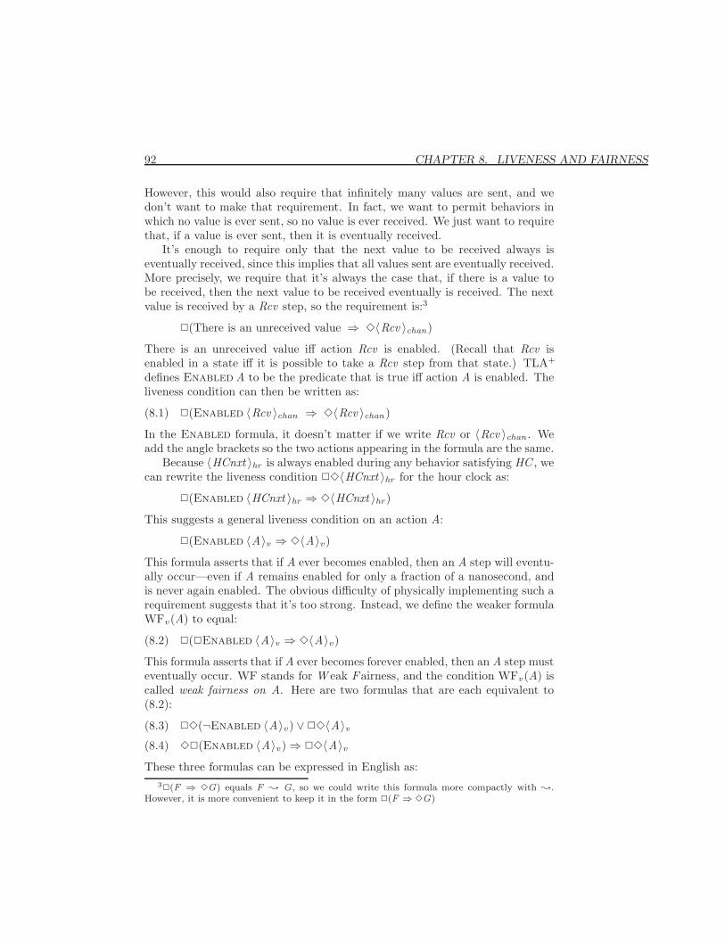
92 CHAPTER 8. LIVENESS AND FAIRNESS
However, this would also require that infinitely many values are sent, and wedon’t want to make that requirement. In fact, we want to permit behaviors inwhich no value is ever sent, so no value is ever received. We just want to requirethat, if a value is ever sent, then it is eventually received.
It’s enough to require only that the next value to be received always iseventually received, since this implies that all values sent are eventually received.More precisely, we require that it’s always the case that, if there is a value tobe received, then the next value to be received eventually is received. The nextvalue is received by a Rcv step, so the requirement is:3
2(There is an unreceived value ⇒ 3〈Rcv 〉chan)
There is an unreceived value iff action Rcv is enabled. (Recall that Rcv isenabled in a state iff it is possible to take a Rcv step from that state.) TLA+
defines Enabled A to be the predicate that is true iff action A is enabled. Theliveness condition can then be written as:
2(Enabled 〈Rcv 〉chan ⇒ 3〈Rcv 〉chan)(8.1)
In the Enabled formula, it doesn’t matter if we write Rcv or 〈Rcv 〉chan . Weadd the angle brackets so the two actions appearing in the formula are the same.
Because 〈HCnxt 〉hr is always enabled during any behavior satisfying HC , wecan rewrite the liveness condition 23〈HCnxt 〉hr for the hour clock as:
2(Enabled 〈HCnxt 〉hr ⇒ 3〈HCnxt 〉hr )This suggests a general liveness condition on an action A:
2(Enabled 〈A〉v ⇒ 3〈A〉v)
This formula asserts that if A ever becomes enabled, then an A step will eventu-ally occur—even if A remains enabled for only a fraction of a nanosecond, andis never again enabled. The obvious difficulty of physically implementing such arequirement suggests that it’s too strong. Instead, we define the weaker formulaWFv (A) to equal:
2(2Enabled 〈A〉v ⇒ 3〈A〉v)(8.2)
This formula asserts that if A ever becomes forever enabled, then an A step musteventually occur. WF stands for W eak Fairness, and the condition WFv (A) iscalled weak fairness on A. Here are two formulas that are each equivalent to(8.2):
23(¬Enabled 〈A〉v ) ∨ 23〈A〉v(8.3)
32(Enabled 〈A〉v )⇒ 23〈A〉v(8.4)
These three formulas can be expressed in English as:32(F ⇒ 3G) equals F ; G, so we could write this formula more compactly with ;.
However, it is more convenient to keep it in the form 2(F ⇒ 3G)
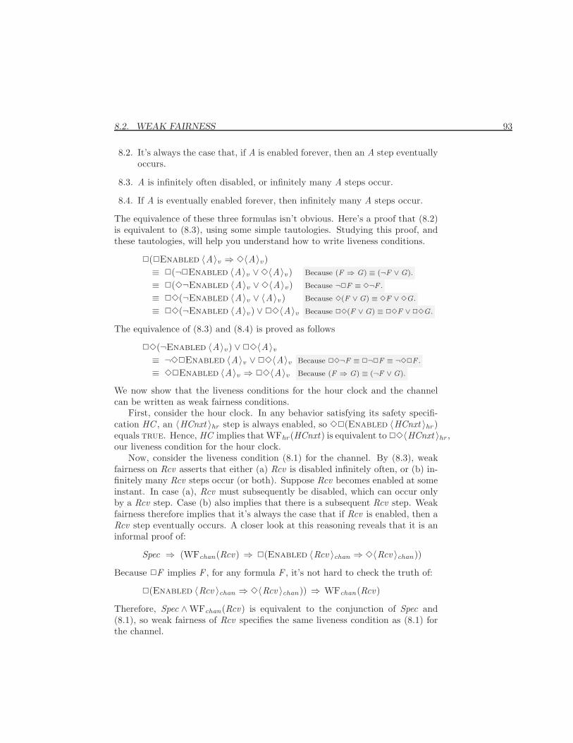
8.2. WEAK FAIRNESS 93
8.2. It’s always the case that, if A is enabled forever, then an A step eventuallyoccurs.
8.3. A is infinitely often disabled, or infinitely many A steps occur.
8.4. If A is eventually enabled forever, then infinitely many A steps occur.
The equivalence of these three formulas isn’t obvious. Here’s a proof that (8.2)is equivalent to (8.3), using some simple tautologies. Studying this proof, andthese tautologies, will help you understand how to write liveness conditions.
2(2Enabled 〈A〉v ⇒ 3〈A〉v)≡ 2(¬2Enabled 〈A〉v ∨3〈A〉v ) Because (F ⇒ G) ≡ (¬F ∨ G).
≡ 2(3¬Enabled 〈A〉v ∨3〈A〉v ) Because ¬2F ≡ 3¬F .
≡ 23(¬Enabled 〈A〉v ∨ 〈A〉v ) Because 3(F ∨ G) ≡ 3F ∨ 3G.
≡ 23(¬Enabled 〈A〉v ) ∨ 23〈A〉v Because 23(F ∨ G) ≡ 23F ∨ 23G.
The equivalence of (8.3) and (8.4) is proved as follows
23(¬Enabled 〈A〉v ) ∨ 23〈A〉v≡ ¬32Enabled 〈A〉v ∨ 23〈A〉v Because 23¬F ≡ 2¬2F ≡ ¬32F .
≡ 32Enabled 〈A〉v ⇒ 23〈A〉v Because (F ⇒ G) ≡ (¬F ∨ G).
We now show that the liveness conditions for the hour clock and the channelcan be written as weak fairness conditions.
First, consider the hour clock. In any behavior satisfying its safety specifi-cation HC , an 〈HCnxt 〉hr step is always enabled, so 32(Enabled 〈HCnxt 〉hr )equals true. Hence, HC implies that WFhr (HCnxt) is equivalent to 23〈HCnxt 〉hr ,our liveness condition for the hour clock.
Now, consider the liveness condition (8.1) for the channel. By (8.3), weakfairness on Rcv asserts that either (a) Rcv is disabled infinitely often, or (b) in-finitely many Rcv steps occur (or both). Suppose Rcv becomes enabled at someinstant. In case (a), Rcv must subsequently be disabled, which can occur onlyby a Rcv step. Case (b) also implies that there is a subsequent Rcv step. Weakfairness therefore implies that it’s always the case that if Rcv is enabled, then aRcv step eventually occurs. A closer look at this reasoning reveals that it is aninformal proof of:
Spec ⇒ (WFchan(Rcv) ⇒ 2(Enabled 〈Rcv 〉chan ⇒ 3〈Rcv 〉chan))
Because 2F implies F , for any formula F , it’s not hard to check the truth of:
2(Enabled 〈Rcv 〉chan ⇒ 3〈Rcv 〉chan)) ⇒ WFchan(Rcv)
Therefore, Spec ∧WFchan(Rcv) is equivalent to the conjunction of Spec and(8.1), so weak fairness of Rcv specifies the same liveness condition as (8.1) forthe channel.
94 CHAPTER 8. LIVENESS AND FAIRNESS
8.3 Liveness for the Memory Specification
Let’s now strengthen the memory specification with the liveness requirementthat every request must receive a response. (We don’t require that a requestis ever issued.) The liveness requirement is conjoined to the internal memoryspecification, formula ISpec of module InternalMemory (Figures 5.2 and 5.3 onpages 52–53).
We will express the liveness requirement in terms of weak fairness. Thisrequires understanding when actions are enabled. The action Rsp(p) is enabledonly if the action
Reply(p, buf [p], memInt , memInt ′)(8.5)
is enabled. Recall that the operator Reply is a constant parameter, declared inthe MemoryInterface module (Figure 5.1 on page 48). Without knowing moreabout this operator, we can’t say when action (8.5) is enabled.
Let’s assume that Reply actions are always enabled. That is, for any pro-cessor p and reply r , and any old value miOld of memInt , there is a new valuemiNew of memInt such that Repl(p, r ,miOld ,miNew) is true. For simplicity,we just assume that this is true for all p and r , and add the following assumptionto the MemoryInterface module:
assume ∀ p, r ,miOld : ∃miNew : Repl(p, r ,miOld ,miNew)
We should also make a similar assumption for Send , but we don’t need it here.We will subscript our weak-fairness formulas with the tuple of all variables,
so let’s add the following definition to the InternalMemory module:
vars ∆= 〈memInt , mem, ctl , buf 〉When processor p issues a request, it enables the Do(p) action, which remains
enabled until a Do(p) step occurs. The weak-fairness condition WFvars(Do(p))implies that this Do(p) step must eventually occur. A Do(p) step enables theRsp(p) action, which remains enabled until an Rsp(p) step occurs. The weak-fairness condition WFvars(Rsp(p)) implies that this Rsp(p) step, which producesthe desired response, must eventually occur. Hence, the requirement
WFvars(Do(p)) ∧WFvars(Rsp(p))(8.6)
assures that every request issued by processor p must eventually receive a reply.We can rewrite condition (8.6) in the slightly simpler form of weak fairness
on the action Do(p) ∨Rsp(p). The disjunction of two actions is enabled iff oneor both of them are enabled. A Req(p) step enables Do(p), thereby enablingDo(p) ∨ Rsp(p). The only Do(p) ∨ Rsp(p) step then possible is a Do(p) step,which enables Rsp(p) and hence Do(p)∨Rsp(p). At this point, the only Do(p)∨Rsp(p) step possible is a Rsp(p) step, which disables Rsp(p) and leaves Do(p)
8.4. STRONG FAIRNESS 95
disabled, hence disabling Do(p)∨Rsp(p). This all shows that (8.6) is equivalentto WFvars(Do(p) ∨Rsp(p)), weak fairness on the single action Do(p) ∨Rsp(p).
Weak fairness of Do(p) ∨Rsp(p) guarantees that every request by processorp receives a response. We want every request from every processor to receive aresponse. So, the liveness condition for the memory specification asserts weakfairness of Do(p) ∨ Rsp(p) for every processor p:4
Liveness ∆= ∀ p ∈ Proc : WFvars(Do(p) ∨ Rsp(p))
The example of actions Do(p) and Rsp(p) raises the general question: whenis the conjunction of weak fairness on actions A1, . . . , An equivalent to weakfairness of their disjunction A1 ∨ . . . ∨ An? The general answer is complicated,but here’s a sufficient condition:
WF Conjunction Rule If A1, . . . , An are actions such that, for anydistinct i and j , whenever action Ai is enabled, action Aj cannot be-come enabled until an Ai step occurs, then WFv (A1) ∧ . . . ∧WFv (An) isequivalent to WFv (A1 ∨ . . . ∨ An).
This rule is stated rather informally. It can be interpreted as an assertion abouta particular behavior σ, in which case its conclusion is
σ |= (WFv (A1) ∧ . . . ∧WFv (An)) ≡ WFv (A1 ∨ . . . ∨ An)
Alternatively, it can be formalized as the assertion that if a formula F impliesthe hypothesis, then F implies the equivalence of WFv (A1) ∧ . . . ∧WFv (An)and WFv (A1 ∨ . . . ∨ An).
Conjunction and disjunction are special cases of universal and existentialquantification, respectively. For example, A1 ∨ . . . ∨ An is equivalent to ∃ i ∈ 1 . . n : Ai .So, we can trivially restate the WF Conjunction Rule as a condition on when∀ i ∈ S : WFv (Ai) and WFv (∃ i ∈ S : Ai) are equivalent, for a finite set S . Theresulting rule is actually valid for any set S :
WF Quantifier Rule If the Ai are actions, for all i ∈ S , such that,for any distinct i and j in S , whenever action Ai is enabled, action Aj
cannot become enabled until an Ai step occurs, then ∀ i ∈ S : WFv (Ai)and WFv (∃ i ∈ S : Ai) are equivalent.
8.4 Strong Fairness
Formulations (8.3) and (8.4) of WFv (A) contain the operators infinitely often(23) and eventually always (32). Eventually always is stronger than (implies)
4Although we haven’t yet discussed quantification in temporal formulas, the meaning ofthe formula ∀ p ∈ Proc : . . . should be clear.
96 CHAPTER 8. LIVENESS AND FAIRNESS
infinitely often. We define SFv (A), strong fairness of action A, to be either ofthe following equivalent formulas:
32(¬Enabled 〈A〉v ) ∨ 23〈A〉v(8.7)
23Enabled 〈A〉v ⇒ 23〈A〉v(8.8)
Intuitively, these two formulas assert:
(8.7) A is eventually disabled forever, or infinitely many A steps occur.
(8.8) If A is infinitely often enabled, then infinitely many A steps occur.
The proof that these two formulas are equivalent is similar to the proof of equiv-alence of (8.3) and (8.4).
The analogs of the WF Conjunction and WF Quantifier Rules (page 95) holdfor strong fairness—for example:
SF Conjunction Rule If A1, . . . , An are actions such that, for anydistinct i and j , whenever action Ai is enabled, action Aj cannot be-come enabled until an Ai step occurs, then SFv (A1) ∧ . . . ∧ SFv (An) isequivalent to SFv (A1 ∨ . . . ∨ An).
It’s not hard to see that strong fairness is stronger than weak fairness—thatis, SFv (A) implies WFv (A), for any v and A. We can express weak and strongfairness as follows.
• Weak fairness of A asserts that an A step must eventually occur if A iscontinuously enabled.
• Strong fairness of A asserts that an A step must eventually occur if A iscontinually enabled.
Continuously means without interruption. Continually means repeatedly, pos-sibly with interruptions.
Strong fairness need not be strictly stronger than weak fairness. Weak andstrong fairness of an action A are equivalent iff A infinitely often disabled impliesthat either A is eventually always disabled, or infinitely many A steps occur.This is expressed formally by the tautology:
(WFv (A) ≡ SFv (A)) ≡(23(¬Enabled 〈A〉v )⇒ 32(¬Enabled 〈A〉v ) ∨ 23〈A〉v )
In the channel example, weak and strong fairness of Rcv are equivalent becauseSpec implies that, once enabled, Rcv can be disabled only by a Rcv step; so ifit is disabled infinitely often, then it either eventually remains disabled forever,or else it is disabled infinitely often by Rcv steps.
Strong fairness can be more difficult to implement than weak fairness, and itis a less common requirement. A strong fairness condition should be used in a
8.5. LIVENESS FOR THE WRITE-THROUGH CACHE 97
specification only if it is needed. When strong and weak fairness are equivalent,the fairness property should be written as weak fairness.
Liveness properties can be subtle. Expressing them with ad hoc temporalformulas can lead to errors. We will specify liveness as the conjunction of fair-ness properties whenever possible—and it almost always is possible. Having auniform way of expressing liveness makes specifications easier to understand.Section 8.7.2 discusses an even more compelling reason for using fairness tospecify liveness.
8.5 Liveness for the Write-Through Cache
Let’s now add liveness to the write-through cache, specified in Figures 5.5–5.7on pages 56–58. We want our specification to guarantee that every request even-tually receives a response, without requiring that any requests are issued. Thisrequires fairness on all the actions that make up the next-state action Next ex-cept the Req(p) action (which issues a request) and the Evict(p, a) action (whichevicts an address from the cache). If any other action were ever enabled withoutbeing executed, then some request might not generate a response—except forone special case. If the memQ queue contains only write requests, and memQ isnot full (has fewer than QLen elements), then not executing a MemQWr actionwould not prevent any responses. (Remember that a response to a write re-quest can be issued before the value is written to memory.) We’ll return to thisexception later. For simplicity, let’s require fairness for the MemQWr actiontoo.
Our liveness condition has to assert fairness of the following actions:
MemQWr MemQRd Rsp(p) RdMiss(p) DoRd(p) DoWr(p)
for all p in Proc. We now must decide whether to assert weak or strong fairnessfor these actions. Weak and strong fairness are equivalent for an action that,once enabled, remains enabled until it is executed. This is the case for all of theseactions except RdMiss(p) and DoWr(p). These two actions append a requestto the memQ queue, and are disabled if that queue is full. A RdMiss(p) orDoWr(p) could be enabled, and then become disabled because a RdMiss(q) orDoWr(q), for a different processor q, appends a request to memQ . We thereforeneed strong fairness for the RdMiss(p) and DoWr(p) actions. So, the fairnessconditions we need are:
Weak Fairness Rsp(p), DoRd(p), MemQWr , and MemQRd
Strong Fairness RdMiss(p) and DoWr(p)
As before, let’s define vars to be the tuple of all variables.
vars ∆= 〈memInt , mem, buf , ctl , cache, memQ 〉
98 CHAPTER 8. LIVENESS AND FAIRNESS
We could just write the liveness condition as
∧ ∀ p ∈ Proc : ∧ WFvars(Rsp(p)) ∧ WFvars(DoRd(p))∧ SFvars(RdMiss(p)) ∧ SFvars(DoWr(p))
∧ WFvars(MemQWr) ∧ WFvars(MemQRd)
(8.9)
However, I prefer replacing the conjunction of fairness conditions by a singlefairness condition on a disjunction, as we did in Section 8.3 for the memoryspecification. The WF and SF Conjunction Rules (page 8.3 and 8.4) easilyimply that the liveness condition (8.9) can be rewritten as
∧ ∀ p ∈ Proc : ∧ WFvars(Rsp(p) ∨DoRd(p))∧ SFvars(RdMiss(p) ∨DoWr(p))
∧ WFvars(MemQWr ∨MemQRd)
(8.10)
We can now try to simplify (8.10) by applying the WF Quantifier Rule (page 95)to replace ∀ p ∈ Proc : WFvars(. . .) with WFvars(∃ p ∈ Proc : . . .). However, thatrule doesn’t apply; it’s possible for Rsp(p) ∨DoRd(p) to be enabled for two dif-ferent processors p at the same time. In fact, the two formulas are not equivalent.Similarly, the analogous rule for strong fairness doesn’t apply. Formula (8.10) isas simple as we can make it.
Let’s return to the observation that we don’t have to execute MemQWr if thememQ queue is not full and contains only write requests. Let’s define QCondto be the assertion that memQ is not full and contains only write requests:
QCond ∆= ∧ Len(memQ) < QLen∧ ∀ i ∈ 1 . . Len(memQ) : memQ [i ][2].op = “Wr”
We have to eventually execute a MemQWr action only when it’s enabled andQCond is true, which is the case iff the action QCond ∧MemQWr is enabled.In this case, a MemQWr step is a QCond ∧MemQWr step. Hence, it sufficesto require weak fairness of the action QCond ∧ MemQWr . We can thereforereplace the second conjunct of (8.10) with
WFvars((QCond ∧MemQWr) ∨ MemQRd)
We would do this if we wanted the specification to describe the weakest livenesscondition that implements the memory specification’s liveness condition. How-ever, if the specification were a description of an actual device, then that devicewould probably implement weak fairness on all MemQWr actions, so we wouldtake (8.10) as the liveness condition.
8.6 Quantification
I’ve already mentioned, in Section 8.1, that the ordinary quantifiers of predicatelogic can be applied to temporal formulas. For example, the meaning of the
8.6. QUANTIFICATION 99
formula ∃ r : F , for any temporal formula F , is given by
σ |= (∃ r : F ) ∆= ∃ r : (σ |= F )
where σ is any behavior. The meaning of ∀ r : F is similarly defined.The symbol r in ∃ r : F is usually called a bound variable. But we’ve been
using the term variable to mean something else—something that’s declared by avariable statement in a module. The bound “variable” r is actually a constantin these formulas—a value that is the same in every state of the behavior.5 Forexample, the formula ∃ r : 2(x = r) asserts that x always has the same value.
The bounded quantifiers are defined in a similar way—for example,
σ |= (∃ r ∈ S : F ) ∆= ∃ r ∈ S : (σ |= F )
For this formula to make sense, S must be a constant.6 The symbol r is declaredto be a constant in formula F . The expression S lies outside the scope of thedeclaration of r , so the symbol r cannot occur in S .
One can, in a similar way, define choose to be a temporal operator. How-ever, it’s not needed for writing specifications, so we won’t.
We have been using the operator ∃∃∃∃∃∃ as a hiding operator. Intuitively, ∃∃∃∃∃∃ x : Fmeans F with variable x hidden. In this formula, x is declared to be a variablein formula F . Unlike ∃ r : F , which asserts the existence of a single value r , theformula ∃∃∃∃∃∃ x : F asserts the existence of a value for x in each state of a behavior.
The precise definition of ∃∃∃∃∃∃ is a bit tricky because, as discussed in Section 8.1,the formula ∃∃∃∃∃∃ x : F should be invariant under stuttering. To define it, we firstdefine σ∼x τ to be true iff σ can be obtained from τ (or vice-versa) by addingand/or removing stuttering steps and changing the values assigned to x by itsstates. To define ∼x precisely, we define two behaviors σ and τ to be stuttering-equivalent iff removing all stuttering steps from each of them produces the samesequence of states. Next, let σx←0 be the behavior that is the same as σ exceptthat, in each state, x is assigned the value 0.7 We can then define σ∼x τ to betrue iff σx←0 and τx←0 are stuttering equivalent. Finally, the meaning of ∃∃∃∃∃∃ isdefined by letting σ |= (∃∃∃∃∃∃ x : F ) be true iff there exists some behavior τ suchthat τ ∼x σ and τ |= F are true. If you find this too confusing, don’t worryabout it. For writing specifications, it suffices to just think of ∃∃∃∃∃∃ x : F as F withx hidden.
TLA also has a temporal universal quantifier ∀∀∀∀∀∀ , defined by:
∀∀∀∀∀∀ x : F ∆= ¬∃∃∃∃∃∃ x : ¬F5Logicians use the term flexible variable for a TLA variable, and the term rigid variable
for a symbol like r that represents a constant.6We can let ∃ r ∈ S : F equal ∃ r : (r ∈ S) ∧ F , which makes sense if S is a state function,
not just a constant. However, TLA+ requires S to be a constant in ∃ r ∈ S : F . If you want itto be a state function, you have to write ∃ r : (r ∈ S) ∧ F .
7The use of 0 is arbitrary; any fixed value would do.
100 CHAPTER 8. LIVENESS AND FAIRNESS
This operator is hardly ever used.TLA+ does not allow bounded versions of the operators ∃∃∃∃∃∃ and ∀∀∀∀∀∀ . If you
want to write ∃∃∃∃∃∃ x ∈ S : F , you can simply write ∃∃∃∃∃∃ x : (x ∈ S ) ∧ F instead.
8.7 Temporal Logic Examined
8.7.1 A Review
Let’s look at the shapes of the specifications that we’ve written so far. Westarted with the simple form
Init ∧ 2[Next ]vars(8.11)
where Init is the initial predicate, Next the next-state action, and vars the tupleof all variables. This kind of specification is, in principle, quite straightforward.
We then introduced hiding: using ∃∃∃∃∃∃ to bind variables that should not ap-pear in the specification. Those bound variables, also called hidden or internalvariables, serve only to help describe how the values of the free variables (alsocalled visible variables) change.
Hiding variables is easy enough, and it is mathematically elegant and philo-sophically satisfying. However, in practice, it doesn’t make much difference toa specification. A comment can also tell a reader that a variable should be re-garded as internal. Explicit hiding allows implementation to mean implication.A lower-level specification that describes an implementation can be expected toimply a specification only if the specification’s internal variables, whose valuesdon’t really matter, are explicitly hidden. Otherwise, implementation meansimplementation under a refinement mapping. (See Section 5.8.) However, asexplained in Section 10.8, implementation often involves a refinement of thevisible variables as well.
To express liveness, the specification (8.11) is strengthened to the form
Init ∧ 2[Next ]vars ∧ Liveness(8.12)
where Liveness is the conjunction of formulas of the form WFvars(A) and/orSFvars(A), for actions A. (I’m considering universal quantification to be a formof conjunction.)
8.7.2 Machine Closure
In the specifications of the form (8.12) we’ve written so far, the actions A whosefairness properties appear in formula Liveness have one thing in common: theyare all subactions of the next-state action Next . An action A is a subaction ofNext iff every A step is a Next step. Equivalently, A is a subaction of Next iff A
8.7. TEMPORAL LOGIC EXAMINED 101
implies Next .8 In almost all specifications of the form (8.12), formula Livenessshould be the conjunction of weak and/or strong fairness formulas for subactionsof Next . I’ll now briefly explain why.
When we look at the specification (8.12), we expect Init to constrain theinitial state, Next to constrain what steps may occur, and Liveness to describeonly what must eventually happen. However, consider the following formula
(x = 0) ∧ 2[x ′ = x + 1]x ∧ WFx ((x > 99) ∧ (x ′ = x − 1))(8.13)
The first two conjuncts of (8.13) assert that x is initially 0 and that any stepeither increments x by 1 or leaves it unchanged. Hence, they imply that if xever exceeds 99, then it forever remains greater than 99. The weak fairnessproperty asserts that, if this happens, then x must eventually be decrementedby 1—contradicting the second conjunct. Hence, (8.13) implies that x can neverexceed 99, so that formula is equivalent to
(x = 0) ∧ 2[(x < 99) ∧ (x ′ = x + 1)]x
Conjoining the weak fairness property to the first two conjuncts of (8.13) forbidsan x ′ = x + 1 step when x = 99.
A specification of the form (8.12) is called machine closed iff the conjunctLiveness does not constrain the initial state or what steps may occur. A moregeneral way to express this is as follows. Let a finite behavior be a finite sequenceof states.9 We say that a finite behavior σ satisfies a safety property S iff thebehavior obtained by adding infinitely many stuttering steps to the end of σsatisfies S . If S is a safety property, then we define the pair of formulas S , Lto be machine closed iff every finite behavior that satisfies S can be extendedto an infinite behavior that satisfies S ∧ L. We call (8.12) machine closed if thepair Init ∧ 2[Next ]vars , Liveness is machine closed.
We seldom want to write a specification that isn’t machine closed. If wedo write one, it’s usually by mistake. Specification (8.12) is guaranteed to bemachine closed if Liveness is the conjunction of weak and/or strong fairnessproperties for subactions of Next .10 This condition doesn’t hold for specification(8.13), which is not machine closed, because (x > 99) ∧ (x ′ = x − 1) is not asubaction of x ′ = x + 1.
Liveness requirements are philosophically satisfying. A specification of theform (8.11), which specifies only a safety property, allows behaviors in whichthe system does nothing. Therefore, the specification is satisfied by a systemthat does nothing. Expressing liveness requirements with fairness properties is
8A weaker notion of subaction is that A is a subaction of the formula (8.11) iff, in everystate of every behavior satisfying (8.11), if A is enabled then Next ∧ A is enabled.
9A finite behavior therefore isn’t a behavior, which is an infinite sequence of states. Math-ematicians often abuse language in this way.
10More precisely, this is the case for a finite or countably infinite conjunction of propertiesof the form WFv (A) and/or SFv (A), where each 〈A〉v is a subaction of Next . This result alsoholds for the weaker definition of subaction in the footnote on this page.
102 CHAPTER 8. LIVENESS AND FAIRNESS
less satisfying. These properties are subtle and it’s easy to get them wrong.It requires some thought to determine that the liveness condition for the write-through cache, formula (8.10) on page 98, does imply that every request receivesa reply.
It’s tempting to express liveness properties more directly, without using fair-ness properties. For example, it’s easy to write a temporal formula asserting forthe write-through cache that every request receives a response. When processorp issues a request, it sets ctl [p] to “rdy”. We just have to assert that a state inwhich ctl [p] = “rdy” is true leads to a Rsp(p) step—for every processor p:
∀ p ∈ Proc : (ctl [p] = “rdy”) ; 〈Rsp(p)〉vars(8.14)
(The operator ; is defined on page 90.) While such formulas are appealing,they are dangerous. It’s very easy to make a mistake and write a specificationthat isn’t machine closed.
Except in unusual circumstances, you should express liveness with fairnessproperties for subactions of the next-state action. These are the most straight-forward specifications, and hence the easiest to write and to understand. Mostsystem specifications, even if very detailed and complicated, can be written inthis straightforward manner. The exceptions are usually in the realm of subtle,high-level specifications that attempt to be very general. An example of such aspecification is given in Section 11.2.
8.7.3 Machine Closure and Possibility
Machine closure can be thought of as a possibility condition. For example,machine closure of the pair S , 23〈A〉v asserts that for every finite behaviorσ satisfying S , it is possible to extended σ to an infinite behavior satisfyingS in which infinitely many 〈A〉v actions occur. If we regard S as a systemspecification, so a behavior that satisfies S represents a possible execution of thesystem, then we can restate machine closure of S , 23〈A〉v as follows: in anysystem execution, it is always possible for infinitely many 〈A〉v actions to occur.
TLA specifications express safety and liveness properties, not possibilityproperties. A safety property asserts that something is impossible—for exam-ple, the system cannot take a step that doesn’t satisfy the next-state action. Aliveness property asserts that something must eventually happen. System re-quirements are sometimes stated informally in terms of what is possible. Mostof the time, when examined rigorously, these requirements can be expressed withliveness and/or safety properties. (The most notable exceptions are statisticalproperties, such as assertions about the probability that something happens.)We are never interested in specifying that something might happen. It’s neveruseful to know that the system might produce the right answer. We never haveto specify that the user might type an “a”; we must specify what happens if hedoes.
8.7. TEMPORAL LOGIC EXAMINED 103
Machine closure is a property of a pair of formulas, not of a system. Althougha possibility property is never a useful assertions about a system, it can bea useful assertion about a specification. A specification S of a system withkeyboard input should always allow a the user to type an “a”. So, we want everyfinite behavior satisfying S to be extendable to an infinite behavior satisfying Sin which infinitely many “a”s are typed. If the action 〈A〉v represents the typingof an “a”, then saying that the user should always be able to type infinitely many“a”s is equivalent to saying that the pair S , 23〈A〉v should be machine closed.If S , 23〈A〉v isn’t machine closed, then it could become impossible for the userever to type an “a”. Unless the system is allowed to lock the keyboard, thismeans that there is something wrong with our specification.
This kind of possibility property can be proved. For example, to prove thatit’s always possible for the user to type infinitely many “a”s, we show thatconjoining suitable fairness conditions on the input actions implies that theuser must type infinitely many “a”s. However, proofs of this kind of simpleproperty don’t seem to be worth the effort. When writing a specification, youshould make sure that possibilities allowed by the real system are allowed by thespecification. Once you are aware of what should be possible, you will usuallyhave little trouble ensuring that the specification makes it possible. You shouldalso make sure that what the system must do is implied by the specification’sfairness conditions. This can be more difficult.
8.7.4 The Unimportance of Liveness
While philosophically important, in practice the liveness property of (8.12) isnot as important as the safety part: Init ∧2[Next ]vars . The ultimate purposeof writing a specification is to avoid errors. Experience shows that most of thebenefit from writing and using a specification comes from the safety part. Onthe other hand, the liveness property is usually easy enough to write. It typicallyconstitutes less than five percent of a specification. So, you might as well writethe liveness part. However, when looking for errors, most of your effort shouldbe devoted to examining the safety part.
8.7.5 Temporal Logic Considered Confusing
The most general type of specification I’ve discussed so far has the form
∃∃∃∃∃∃ v1, . . . , vn : Init ∧ 2[Next ]vars ∧ Liveness(8.15)
where Liveness is the conjunction of fairness properties of subactions of Next .This is a very restricted class of temporal-logic formulas. Temporal logic is quiteexpressive, and one can combine its operators in all sorts of ways to express awide variety of properties. This suggests the following approach to writing a
104 CHAPTER 8. LIVENESS AND FAIRNESS
specification: express each property that the system must satisfy with a temporalformula, and then conjoin all these formulas. For example, formula (8.14) aboveexpresses the property of the write-through cache that every request eventuallyreceives a response.
This approach is philosophically appealing. It has just one problem: it’spractical for only the very simplest of specifications—and even for them, it sel-dom works well. The unbridled use of temporal logic produces formulas that arehard to understand. Conjoining several of these formulas produces a specifica-tion that is impossible to understand.
The basic form of a TLA specification is (8.15). Most specifications shouldhave this form. We can also use this kind of specification as a building block.Chapters 9 and Section 10 describe situations in which we write a specification asa conjunction of such formulas. Section 10.7 introduces an additional temporaloperator +−. and explains why we might want to write a specification F +−. G,where F and G have the form (8.12). But such specifications are of limitedpractical use. Most engineers need only know how to write specifications of theform (8.15). Indeed, they can get along quite well with specifications of the form(8.11) that express only safety properties.
Chapter 9
Real Time
9.1 The Hour Clock Revisited
Let’s return to our specification of the simple hour clock in Chapter 2, whichasserts that the variable hr cycles through the values 1 through 12. We nowadd the obvious requirement that the clock keep correct time. In science, onerepresents the real-time behavior of a system by introducing a variable, tradi-tionally t , whose value is a real number that represents time. A state in which Remember that a
state is an assign-ment of values toall relevant vari-ables.
t = −17.51 represents a state of the system at time −17.51, perhaps measuredin seconds elapsed since 00:00 UT on 1 January 2000. In TLA+ specifications, Iprefer to use the variable now rather than t . For linguistic convenience, I willusually assume that the unit of time is the second, though we could just as wellchoose any other unit.
Unlike sciences such as physics and chemistry, computer science studies sys-tems whose behavior can be described by a sequence of discrete states, ratherthan by states that vary continuously with time. We consider the hour clock’sdisplay to change directly from reading 12 to reading 1, and ignore the contin-uum of intermediate states that occur in the physical display. This means thatwe pretend that the change is instantaneous. So, a real-time specification of theclock might allow the step[
hr = 12now =
√2.47
]→
[hr = 1now =
√2.47
]
The value of now advances between changes to hr . If we wanted to specify howlong it takes the display to change from 12 to 1, we would have to introducean intermediate state that represents a changing display—perhaps by letting hrassume some intermediate value such as 12.5, or by adding a Boolean-valuedvariable chg whose value indicates whether the display is changing. We won’t
105
106 CHAPTER 9. REAL TIME
do this, but will be content to specify an hour clock in which we consider thedisplay to change instantaneously.
The value of now changes between changes to hr . Just as we represent acontinuously varying clock display by a variable whose value changes in discretesteps, we let the value of now change in discrete steps. A behavior in which nowincreases in femtosecond increments would be an accurate enough description ofcontinuously changing time for our specification of the hour clock. In fact, there’sno need to specify any particular granularity of time; we can let now advanceby arbitrary amounts between clock ticks. (Since the value of hr is unchangedby steps that change now , the requirement that the clock keep correct time willrule out behaviors in which now changes by too much in a single step.)
What real-time condition do we want to require for our hour clock? We mightrequire that it always display the correct time. A more realistic requirementwould be that it display the time correctly to within ρ seconds, for some realnumber ρ. However, this is not typical of the real-time requirements that arisein actual systems. Instead, we require that the clock tick approximately onceper hour. More precisely, we require that the interval between ticks be one hourplus or minus ρ seconds, for some positive number ρ. Of course, this requirementallows the time displayed by the clock eventually to drift away from the actualtime. But that’s what most real clocks will do if not reset.
We could start our specification of the real-time clock from scratch. How-ever, we still want the hour clock to satisfy the specification HC of moduleHourClock (Figure 2.1 on page 20). We just want to add an additional real-timerequirement. So, we will write the specification as the conjunction of HC and aformula requiring that the clock tick every hour, plus or minus ρ seconds. Thisrequirement is the conjunction of two separate requirements: that the clock tickat most once every 3600− ρ seconds, and at least once every 3600 + ρ seconds.
To specify these requirements, we must introduce a variable that records howmuch time has elapsed since the last clock tick. Let’s call it t for timer . Thevalue of t is set to 0 by a step that represents a clock tick—namely, by an HCnxtstep. Any step that represents the passing of s seconds should advance t by s . Astep represents the passing of time iff it changes now , and such step representsthe passage of now ′ − now seconds. So, the change to the timer t is describedby the action:
TNext ∆= t ′ = if HCnxt then 0 else t + (now ′ − now)
The specification of how t changes is a formula asserting that every step is aTNext step or else leaves t and now unchanged. Letting t initially equal 0 (sowe start in a state in which the clock has just ticked), this formula is:
Timer ∆= (t = 0) ∧ 2[TNext ]〈t, hr 〉
The requirement that the clock tick at least once every 3600 + ρ seconds meansthat it’s always the case that at most 3600 + ρ seconds have elapsed since the
9.1. THE HOUR CLOCK REVISITED 107
last HCnxt step. Since t always equals the elapsed time since the last HCnxtstep, this requirement is expressed by the formula:
MaxTime ∆= 2(t ≤ 3600 + ρ)
(Since we can’t measure time with perfect accuracy, it doesn’t matter whetherwe use < or ≤. When we generalize from this example, it will be somewhatmore convenient to use ≤.)
The requirement that the clock tick at most once every 3600 − ρ secondsmeans that, whenever an HCnxt step occurs, at least 3600 − ρ seconds haveelapsed since the previous HCnxt step. This suggests the condition In the general-
ization, ≥ will bemore convenientthan >.
2(HCnxt ⇒ (t ≥ 3600− ρ))(9.1)
However, (9.1) isn’t a legal TLA formula because HCnxt ⇒ . . . is an action(a formula containing primes), and a TLA formula asserting that an action isalways true must have the form 2[A]v . We don’t care about steps that leave hrunchanged, so we can replace (9.1) by the TLA formula:
MinTime ∆= 2[HCnxt ⇒ (t ≥ 3600− ρ)]hr
The desired real-time constraint on the clock is expressed by the conjunction ofthese three formulas:
HCTime ∆= Timer ∧ MaxTime ∧ MinTime
However, formula HCTime contains the variable t , and the specification of thereal-time clock should describe only the changes to hr (the clock display) andnow (the time). So, we have to hide t . Hiding is expressed in TLA+ by thetemporal existential quantifier ∃∃∃∃∃∃ , introduced in Section 4.3 (page 41). However,as explained in that section, we can’t simply write ∃∃∃∃∃∃ t : HCTime. We must defineHCTime in a module that declares t , and then use a parametrized instantiationof that module. This is done in Figure 9.1 on page 109. Instead of definingHCTime in a completely separate module, I have defined it in a submodulenamed Inner of the module RealTimeHourClock containing the specification ofthe real-time hour clock. Note that all the symbols declared and defined in themain module up to that point can be used in the submodule. Submodule Inneris instantiated in the main module with the statement
I (t) ∆= instance Inner
The t in HCTime can then be hidden by writing ∃∃∃∃∃∃ t : I (t)!HCTime.The formula HC ∧ (∃∃∃∃∃∃ t : I (t)!HCTime) describes the possible changes to the
value of hr , and relates those changes to the value of now . But it says very littleabout how the value of now can change. For example, it allows the followingbehavior:[
hr = 11now = 23.5
]→
[hr = 11now = 23.4
]→
[hr = 11now = 23.5
]→
[hr = 11now = 23.4
]→ · · ·
108 CHAPTER 9. REAL TIME
Because time can’t go backwards, such a behavior doesn’t represent a physicalpossibility. Everyone knows that time only increases, so there’s no need to forbidthis behavior if the only purpose of our specification is to describe the hour clock.However, a specification should also allow us to reason about a system. If theclock ticks approximately once per hour, then it can’t stop. However, as thebehavior above shows, the formula HC ∧ (∃∃∃∃∃∃ t : I (t)!HCTime) by itself allowsthe clock to stop. To infer that it can’t, we also need to state how now changes.
We define a formula RTnow that specifies the possible changes to now . Thisformula does not specify the granularity of the changes to now ; it allows nowto advance by a microsecond or by a century. However, we have decided that astep that changes hr should leave now unchanged, so a step that changes nowshould leave hr unchanged. Therefore, steps that change now are described bythe action:
NowNext ∆= ∧ now ′ ∈ {r ∈ Real : r > now}∧ unchanged hr
Formula RTnow should also allows steps that leave now unchanged. The initialvalue of now is arbitrary (we can start the system at any time), so the safetypart of RTnow is:
(now ∈ Real) ∧ 2[NowNext ]now
The liveness condition we want is that now should increase without bound.Simple weak fairness of the NowNext action isn’t good enough, because it allows Fairness is dis-
cussed in Chap-ter 8.
“Zeno” behaviors such as:
[now = .9] → [now = .99] → [now = .999] → [now = .9999] → · · ·in which the value of now remains bounded. Weak fairness of the actionNowNext ∧ (now ′ > r) implies that eventually a NowNext step will occur inwhich the new value of now is greater than r . (This action is always enabled, soweak fairness implies that infinitely many such actions must occur.) Assertingthis for all real numbers r implies that now grows without bound, so we take asthe fairness condition:
∀ r ∈ Real : WFnow (NowNext ∧ (now ′ > r))
The complete specification of the real-time hour clock, including the definitionof formula RTnow , appears in Figure 9.1 on the next page.
9.2 Real-Time Specifications in General
In Section 8.2 (page 91), we saw that the appropriate generalization of the live-ness requirement that the hour clock tick infinitely often is weak fairness of the
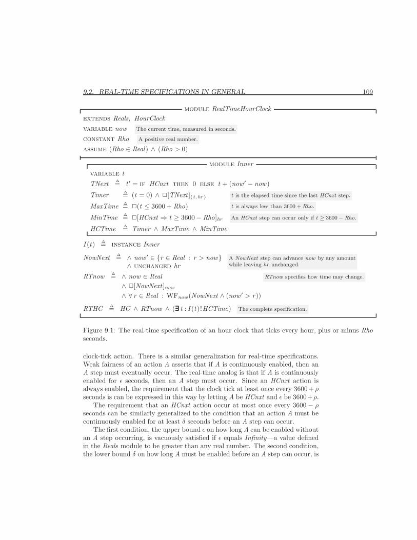
9.2. REAL-TIME SPECIFICATIONS IN GENERAL 109
module RealTimeHourClockextends Reals, HourClockvariable now The current time, measured in seconds.
constant Rho A positive real number.
assume (Rho ∈ Real) ∧ (Rho > 0)
module Innervariable tTNext ∆= t ′ = if HCnxt then 0 else t + (now ′ − now)
Timer ∆= (t = 0) ∧ 2[TNext ]〈t,hr 〉MaxTime ∆= 2(t ≤ 3600 + Rho)
MinTime ∆= 2[HCnxt ⇒ t ≥ 3600− Rho]hrHCTime ∆= Timer ∧ MaxTime ∧ MinTime
t is the elapsed time since the last HCnxt step.
t is always less than 3600 + Rho.
An HCnxt step can occur only if t ≥ 3600 − Rho.
I (t) ∆= instance Inner
NowNext ∆= ∧ now ′ ∈ {r ∈ Real : r > now}∧ unchanged hr
A NowNext step can advance now by any amountwhile leaving hr unchanged.
RTnow ∆= ∧ now ∈ Real∧ 2[NowNext ]now
∧ ∀ r ∈ Real : WFnow (NowNext ∧ (now ′ > r))
RTnow specifies how time may change.
RTHC ∆= HC ∧ RTnow ∧ (∃∃∃∃∃∃ t : I (t)!HCTime) The complete specification.
Figure 9.1: The real-time specification of an hour clock that ticks every hour, plus or minus Rhoseconds.
clock-tick action. There is a similar generalization for real-time specifications.Weak fairness of an action A asserts that if A is continuously enabled, then anA step must eventually occur. The real-time analog is that if A is continuouslyenabled for ε seconds, then an A step must occur. Since an HCnxt action isalways enabled, the requirement that the clock tick at least once every 3600+ ρseconds is can be expressed in this way by letting A be HCnxt and ε be 3600+ρ.
The requirement that an HCnxt action occur at most once every 3600 − ρseconds can be similarly generalized to the condition that an action A must becontinuously enabled for at least δ seconds before an A step can occur.
The first condition, the upper bound ε on how long A can be enabled withoutan A step occurring, is vacuously satisfied if ε equals Infinity—a value definedin the Reals module to be greater than any real number. The second condition,the lower bound δ on how long A must be enabled before an A step can occur, is
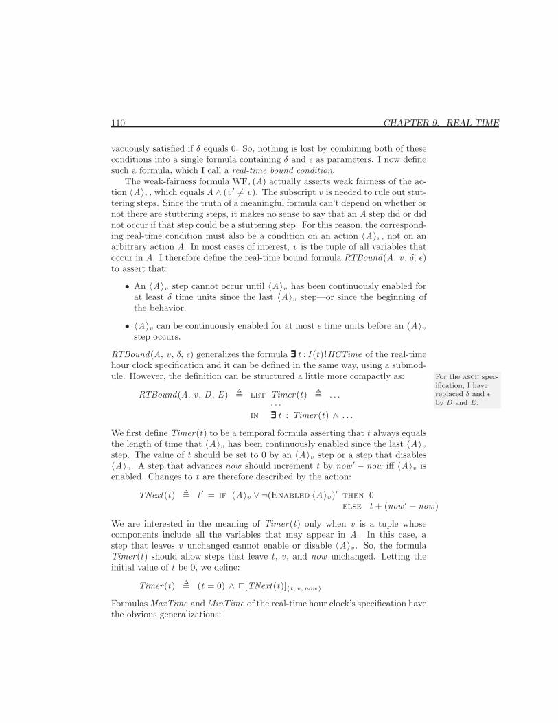
110 CHAPTER 9. REAL TIME
vacuously satisfied if δ equals 0. So, nothing is lost by combining both of theseconditions into a single formula containing δ and ε as parameters. I now definesuch a formula, which I call a real-time bound condition.
The weak-fairness formula WFv (A) actually asserts weak fairness of the ac-tion 〈A〉v , which equals A ∧ (v ′ 6= v). The subscript v is needed to rule out stut-tering steps. Since the truth of a meaningful formula can’t depend on whether ornot there are stuttering steps, it makes no sense to say that an A step did or didnot occur if that step could be a stuttering step. For this reason, the correspond-ing real-time condition must also be a condition on an action 〈A〉v , not on anarbitrary action A. In most cases of interest, v is the tuple of all variables thatoccur in A. I therefore define the real-time bound formula RTBound(A, v , δ, ε)to assert that:
• An 〈A〉v step cannot occur until 〈A〉v has been continuously enabled forat least δ time units since the last 〈A〉v step—or since the beginning ofthe behavior.
• 〈A〉v can be continuously enabled for at most ε time units before an 〈A〉vstep occurs.
RTBound(A, v , δ, ε) generalizes the formula ∃∃∃∃∃∃ t : I (t)!HCTime of the real-timehour clock specification and it can be defined in the same way, using a submod-ule. However, the definition can be structured a little more compactly as: For the ascii spec-
ification, I havereplaced δ and εby D and E .
RTBound(A, v , D , E ) ∆= let Timer(t) ∆= . . .. . .
in ∃∃∃∃∃∃ t : Timer(t) ∧ . . .
We first define Timer(t) to be a temporal formula asserting that t always equalsthe length of time that 〈A〉v has been continuously enabled since the last 〈A〉vstep. The value of t should be set to 0 by an 〈A〉v step or a step that disables〈A〉v . A step that advances now should increment t by now ′ − now iff 〈A〉v isenabled. Changes to t are therefore described by the action:
TNext(t) ∆= t ′ = if 〈A〉v ∨ ¬(Enabled 〈A〉v )′ then 0else t + (now ′ − now)
We are interested in the meaning of Timer(t) only when v is a tuple whosecomponents include all the variables that may appear in A. In this case, astep that leaves v unchanged cannot enable or disable 〈A〉v . So, the formulaTimer(t) should allow steps that leave t , v , and now unchanged. Letting theinitial value of t be 0, we define:
Timer(t) ∆= (t = 0) ∧ 2[TNext(t)]〈t, v , now 〉
Formulas MaxTime and MinTime of the real-time hour clock’s specification havethe obvious generalizations:
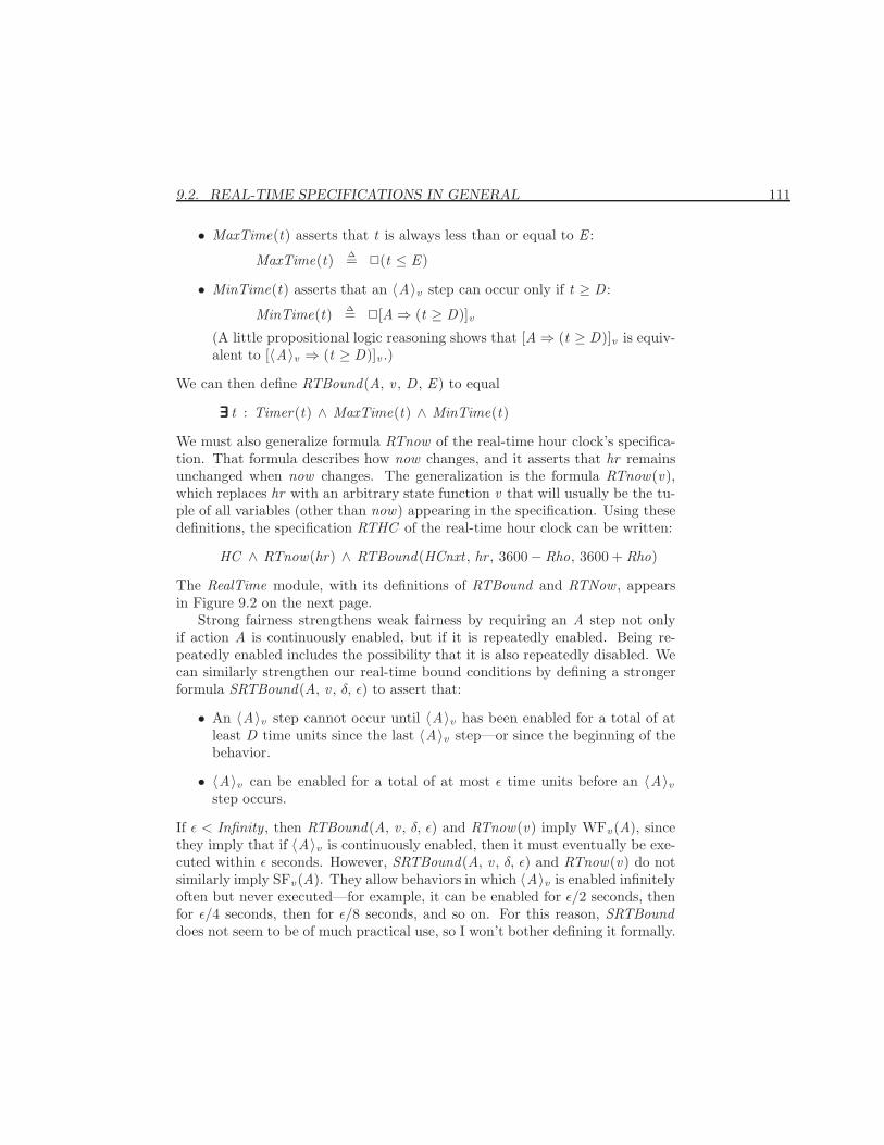
9.2. REAL-TIME SPECIFICATIONS IN GENERAL 111
• MaxTime(t) asserts that t is always less than or equal to E :
MaxTime(t) ∆= 2(t ≤ E )
• MinTime(t) asserts that an 〈A〉v step can occur only if t ≥ D :
MinTime(t) ∆= 2[A⇒ (t ≥ D)]v(A little propositional logic reasoning shows that [A⇒ (t ≥ D)]v is equiv-alent to [〈A〉v ⇒ (t ≥ D)]v .)
We can then define RTBound(A, v , D , E ) to equal
∃∃∃∃∃∃ t : Timer(t) ∧ MaxTime(t) ∧ MinTime(t)
We must also generalize formula RTnow of the real-time hour clock’s specifica-tion. That formula describes how now changes, and it asserts that hr remainsunchanged when now changes. The generalization is the formula RTnow(v),which replaces hr with an arbitrary state function v that will usually be the tu-ple of all variables (other than now) appearing in the specification. Using thesedefinitions, the specification RTHC of the real-time hour clock can be written:
HC ∧ RTnow(hr) ∧ RTBound(HCnxt , hr , 3600− Rho, 3600 + Rho)
The RealTime module, with its definitions of RTBound and RTNow , appearsin Figure 9.2 on the next page.
Strong fairness strengthens weak fairness by requiring an A step not onlyif action A is continuously enabled, but if it is repeatedly enabled. Being re-peatedly enabled includes the possibility that it is also repeatedly disabled. Wecan similarly strengthen our real-time bound conditions by defining a strongerformula SRTBound(A, v , δ, ε) to assert that:
• An 〈A〉v step cannot occur until 〈A〉v has been enabled for a total of atleast D time units since the last 〈A〉v step—or since the beginning of thebehavior.
• 〈A〉v can be enabled for a total of at most ε time units before an 〈A〉vstep occurs.
If ε < Infinity, then RTBound(A, v , δ, ε) and RTnow(v) imply WFv (A), sincethey imply that if 〈A〉v is continuously enabled, then it must eventually be exe-cuted within ε seconds. However, SRTBound(A, v , δ, ε) and RTnow(v) do notsimilarly imply SFv (A). They allow behaviors in which 〈A〉v is enabled infinitelyoften but never executed—for example, it can be enabled for ε/2 seconds, thenfor ε/4 seconds, then for ε/8 seconds, and so on. For this reason, SRTBounddoes not seem to be of much practical use, so I won’t bother defining it formally.
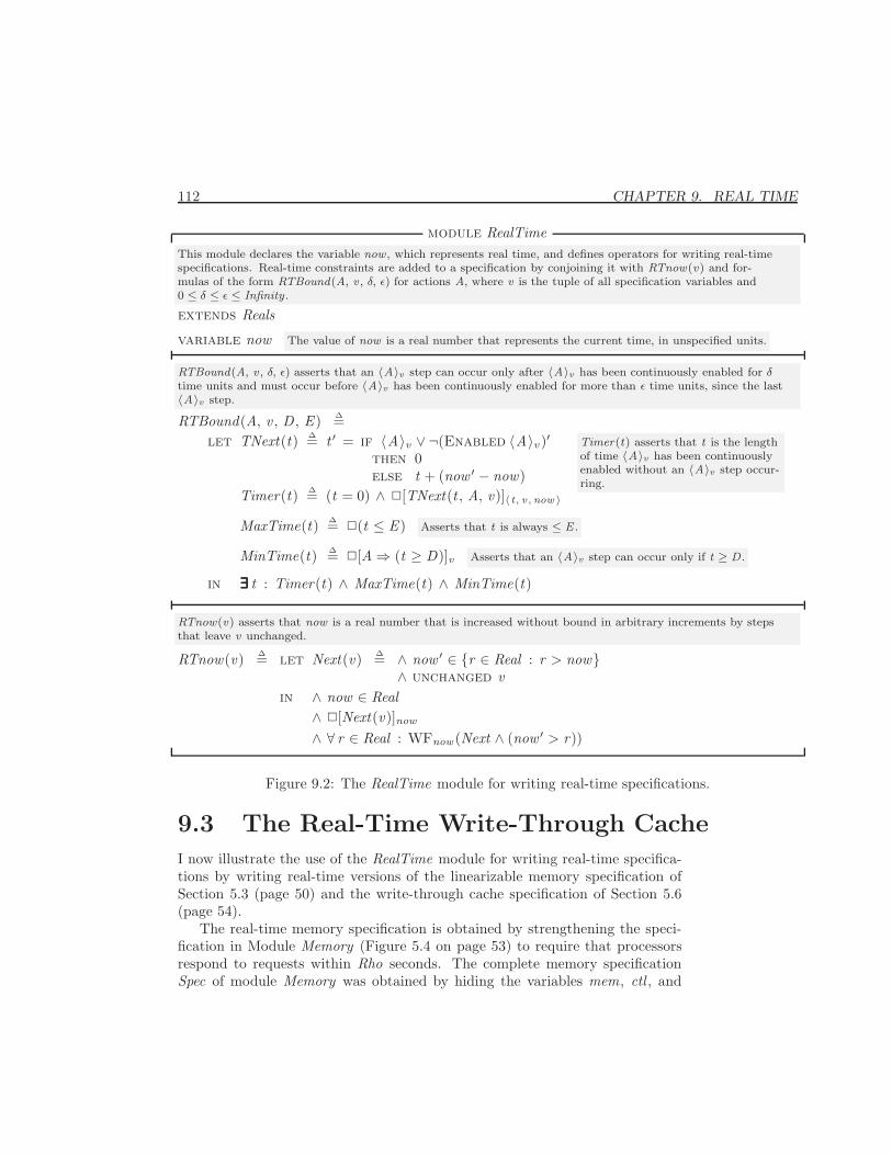
112 CHAPTER 9. REAL TIME
module RealTimeThis module declares the variable now , which represents real time, and defines operators for writing real-timespecifications. Real-time constraints are added to a specification by conjoining it with RTnow(v) and for-mulas of the form RTBound(A, v , δ, ε) for actions A, where v is the tuple of all specification variables and0 ≤ δ ≤ ε ≤ Infinity .
extends Reals
variable now The value of now is a real number that represents the current time, in unspecified units.
RTBound(A, v , δ, ε) asserts that an 〈A〉v step can occur only after 〈A〉v has been continuously enabled for δtime units and must occur before 〈A〉v has been continuously enabled for more than ε time units, since the last〈A〉v step.
RTBound(A, v , D , E ) ∆=let TNext(t) ∆= t ′ = if 〈A〉v ∨ ¬(Enabled 〈A〉v )′
then 0else t + (now ′ − now)
Timer(t) asserts that t is the lengthof time 〈A〉v has been continuouslyenabled without an 〈A〉v step occur-ring.
Timer(t) ∆= (t = 0) ∧ 2[TNext(t , A, v)]〈t, v , now 〉
MaxTime(t) ∆= 2(t ≤ E ) Asserts that t is always ≤ E .
MinTime(t) ∆= 2[A⇒ (t ≥ D)]v Asserts that an 〈A〉v step can occur only if t ≥ D .
in ∃∃∃∃∃∃ t : Timer(t) ∧ MaxTime(t) ∧ MinTime(t)
RTnow(v) asserts that now is a real number that is increased without bound in arbitrary increments by stepsthat leave v unchanged.
RTnow(v) ∆= let Next(v) ∆= ∧ now ′ ∈ {r ∈ Real : r > now}∧ unchanged v
in ∧ now ∈ Real∧ 2[Next(v)]now
∧ ∀ r ∈ Real : WFnow (Next ∧ (now ′ > r))
Figure 9.2: The RealTime module for writing real-time specifications.
9.3 The Real-Time Write-Through Cache
I now illustrate the use of the RealTime module for writing real-time specifica-tions by writing real-time versions of the linearizable memory specification ofSection 5.3 (page 50) and the write-through cache specification of Section 5.6(page 54).
The real-time memory specification is obtained by strengthening the speci-fication in Module Memory (Figure 5.4 on page 53) to require that processorsrespond to requests within Rho seconds. The complete memory specificationSpec of module Memory was obtained by hiding the variables mem, ctl , and
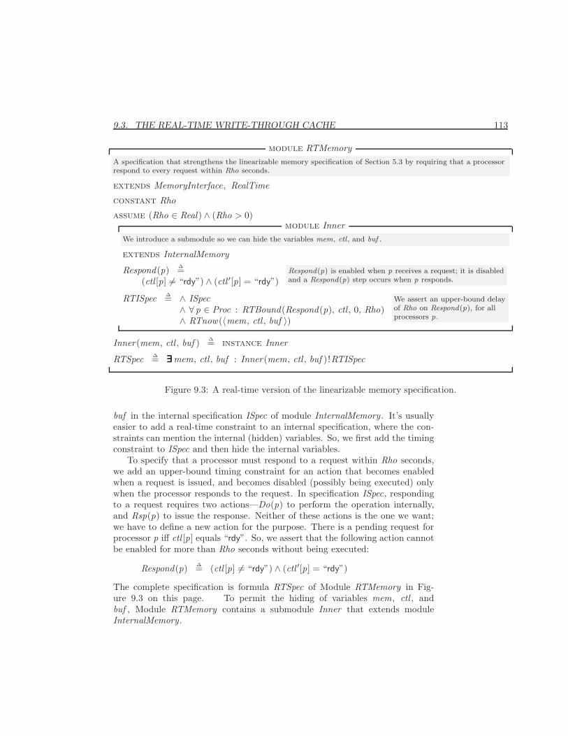
9.3. THE REAL-TIME WRITE-THROUGH CACHE 113
module RTMemoryA specification that strengthens the linearizable memory specification of Section 5.3 by requiring that a processorrespond to every request within Rho seconds.
extends MemoryInterface, RealTime
constant Rho
assume (Rho ∈ Real) ∧ (Rho > 0)module Inner
We introduce a submodule so we can hide the variables mem, ctl , and buf .
extends InternalMemory
Respond(p) ∆=(ctl [p] 6= “rdy”) ∧ (ctl ′[p] = “rdy”)
Respond(p) is enabled when p receives a request; it is disabledand a Respond(p) step occurs when p responds.
RTISpec ∆= ∧ ISpec∧ ∀ p ∈ Proc : RTBound(Respond(p), ctl , 0, Rho)∧ RTnow(〈mem, ctl , buf 〉)
We assert an upper-bound delayof Rho on Respond(p), for allprocessors p.
Inner(mem, ctl , buf ) ∆= instance Inner
RTSpec ∆= ∃∃∃∃∃∃mem, ctl , buf : Inner(mem, ctl , buf )!RTISpec
Figure 9.3: A real-time version of the linearizable memory specification.
buf in the internal specification ISpec of module InternalMemory. It’s usuallyeasier to add a real-time constraint to an internal specification, where the con-straints can mention the internal (hidden) variables. So, we first add the timingconstraint to ISpec and then hide the internal variables.
To specify that a processor must respond to a request within Rho seconds,we add an upper-bound timing constraint for an action that becomes enabledwhen a request is issued, and becomes disabled (possibly being executed) onlywhen the processor responds to the request. In specification ISpec, respondingto a request requires two actions—Do(p) to perform the operation internally,and Rsp(p) to issue the response. Neither of these actions is the one we want;we have to define a new action for the purpose. There is a pending request forprocessor p iff ctl [p] equals “rdy”. So, we assert that the following action cannotbe enabled for more than Rho seconds without being executed:
Respond(p) ∆= (ctl [p] 6= “rdy”) ∧ (ctl ′[p] = “rdy”)
The complete specification is formula RTSpec of Module RTMemory in Fig-ure 9.3 on this page. To permit the hiding of variables mem, ctl , andbuf , Module RTMemory contains a submodule Inner that extends moduleInternalMemory.
114 CHAPTER 9. REAL TIME
Having added a real-time constraint to the specification of a linearizablememory, let’s strengthen the specification of the write-through cache so it sat-isfies that constraint. The object is not just to add any real-time constraintthat does the job—that’s easy to do by using the same constraint that we addedto the memory specification. We want to write a specification of a real-timealgorithm—a specification that tells an implementor how to meet the real-timeconstraints. This is generally done by placing real-time bounds on the actualactions of the untimed specification, not by adding time bounds on a new ac-tion, as we did for the memory specification. An upper-bound constraint on theresponse time should be achieved by enforcing upper-bound constraints on thesystem’s actions.
If we try to achieve a bound on response time by adding real-time boundsto the write-through cache specification’s actions, we encounter the followingproblem. Processors have to “compete” with one another to be able to enqueueoperations on the finite queue memQ . For example, when servicing a writerequest, processor p must execute a DoWr(p) action to enqueue the operationto the tail of memQ . That action is not enabled if memQ is full. The DoWr(p)action can be continually disabled by other processors performing DoWr orRdMiss actions. That’s why, to guarantee liveness—that each request eventuallyreceives a response—in Section 8.5 (page 97) we had to assert strong fairness ofDoWr and RdMiss actions. The only way to ensure that a DoWr(p) action isexecuted within some length of time is to use lower-bound constraints on theactions of other processors to ensure that they cannot perform DoWr or RdMissactions too frequently. Although such a specification is possible, it is not thekind of approach anyone is likely to take in practice.
The usual method of enforcing real-time bounds on accesses to a sharedresource is to schedule the use of the resource by different processors. So, let’smodify the write-through cache to add a scheduling discipline to actions thatenqueue operations on memQ . We use round robin scheduling, which is probablythe easiest one to implement. Suppose processors are numbered from 0 throughN−1. Round-robin scheduling means that processor p is the next processor afterq to enqueue its operation iff none of the processors (q + 1) % N , (q + 2) % N ,. . . , (p − 1) % N is waiting to access memQ .
To express this formally, we first let the set Proc of processors equal theset 0 . . (N − 1) of integers. Normally, this is done by defining Proc to equal0 . . (N −1). However, we want to reuse the parameters and definitions from thewrite-through cache specification. The easiest way to do this is by extendingmodule WriteThroughCache. Since Proc is a parameter in that module, wecan’t define it. We therefore let N be a new constant parameter and let Proc =0 . . (N − 1) be an assumption.1
1We could also instantiate module WriteThroughCache with 0 . . (N − 1) substituted forProc; but that requires declaring the other parameters of WriteThroughCache, including theones from the MemoryInterface module.
9.3. THE REAL-TIME WRITE-THROUGH CACHE 115
To implement round-robin scheduling, we use a variable lastP whose valueis the last processor to enqueue an operation to memQ . We define the operatorposition so that p is the position(p)th processor after lastP in the round-robinorder:
position(p) ∆= choose i ∈ 1 . . N : p = (lastP + 1) % N
Processor p can be the next to access memQ iff no processor q with position(q) <position(p) is ready to access it—that is, iff canGoNext(p) is true, where
canGoNext(p) ∆=∀ q ∈ Proc : (position(q) < position(p)) ⇒ ¬Enabled (RdMiss(q) ∨DoWr(q))
We then define RTRdMiss(p) and RTDoWr(p) to be the same as RdMiss(p) andDoWr(p), respectively, except that they have the additional enabling conditioncanGoNext(p), and they set lastP to p. The other subactions of the next-stateaction are the same as before, except that they must also leave lastP unchanged.
For simplicity, we assume a single upper bound of Epsilon on the lengthof time any of the actions of processor p can remain enabled without beingexecuted—except for the Evict(p, a) action, which we never require to happen.If two actions A and B are never simultaneously enabled, and one must beexecuted before the other can become enabled, then a single real-time constrainton A ∨ B is equivalent to separate constraints on A and B . We can thereforeplace a single constraint on the disjunction of all the actions of processor p,except we can’t use the same constraint for both DoRd(p) and RTRdMiss(p),since an Evict(p, a) step could disable DoRd(p) and enable RTRdMiss(p).
We assume an upper bound of Delta on the time MemQWr or MemQRd canbe enabled without dequeuing an operation from memQ . The variable memQrepresents a physical queue between the bus and the main memory, and Deltamust be large enough so an operation inserted into an empty queue will reachthe memory and be dequeued within Delta seconds.
We want the real-time write-through cache to implement the real-time mem-ory specification. This requires an assumption relating Delta, Epsilon, and Rhoto assure that the memory specification’s timing constraint is satisfied—namely,that the delay between when a processor p receives a request and when it re-sponds is at most Rho. Determining this assumption requires computing anupper bound on that delay. Finding the smallest upper bound is complicated,but it isn’t too hard to show that
(2 ∗N + 1) ∗Delta + (N + QLen) ∗ Epsilon
is an upper bound. So we assume that this value is less than or equal to Rho.The complete specification appears in Figures 9.4 and 9.5 on the following
two pages. The module also asserts as a theorem that the specification RTSpecof the real-time write-through cache implements (implies) the real-time memoryspecification, formula RTSpec of module RTMemory.
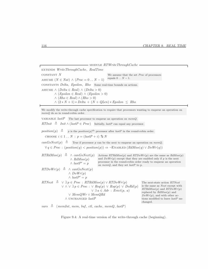
116 CHAPTER 9. REAL TIME
module RTWriteThroughCacheextends WriteThroughCache, RealTimeconstant Nassume (N ∈ Nat) ∧ (Proc = 0 . . N − 1)
We assume that the set Proc of processorsequals 0 . . N − 1.
constants Delta, Epsilon, Rho Some real-time bounds on actions.
assume ∧ (Delta ∈ Real) ∧ (Delta > 0)∧ (Epsilon ∈ Real) ∧ (Epsilon > 0)∧ (Rho ∈ Real) ∧ (Rho > 0)∧ (2 ∗N + 1) ∗Delta + (N + QLen) ∗ Epsilon ≤ Rho
We modify the write-through cache specification to require that processors wanting to enqueue an operation onmemQ do so in round-robin order.
variable lastP The last processor to enqueue an operation on memQ .
RTInit ∆= Init ∧ (lastP ∈ Proc) Initially, lastP can equal any processor.
position(p) ∆= p is the position(p)th processor after lastP in the round-robin order.
choose i ∈ 1 . . N : p = (lastP + i) % N
canGoNext(p) ∆= True if processor p can be the next to enqueue an operation on memQ .
∀ q ∈ Proc : (position(q) < position(p)) ⇒ ¬Enabled (RdMiss(q) ∨DoWr(q))
RTRdMiss(p) ∆= ∧ canGoNext(p)∧ RdMiss(p)∧ lastP ′ = p
Actions RTRdMiss(p) and RTDoWr(p) are the same as RdMiss(p)and DoWr(p) except that they are enabled only if p is the nextprocessor in the round-robin order ready to enqueue an operationon memQ , and they set lastP to p.
RTDoWr(p) ∆= ∧ canGoNext(p)∧ DoWr(p)∧ lastP ′ = p
RTNext ∆= ∨ ∃ p ∈ Proc : RTRdMiss(p) ∨ RTDoWr(p)∨ ∧ ∨ ∃ p ∈ Proc : ∨ Req(p) ∨ Rsp(p) ∨ DoRd(p)
∨ ∃ a ∈ Adr : Evict(p, a)∨ MemQWr ∨MemQRd
∧ unchanged lastP
The next-state action RTNextis the same as Next except withRTRdMiss(p) and RTDoWr(p)replaced by RdMiss(p) andDoWr(p), and with other ac-tions modified to leave lastP un-changed.
vars ∆= 〈memInt , mem, buf , ctl , cache, memQ , lastP 〉
Figure 9.4: A real-time version of the write-through cache (beginning).
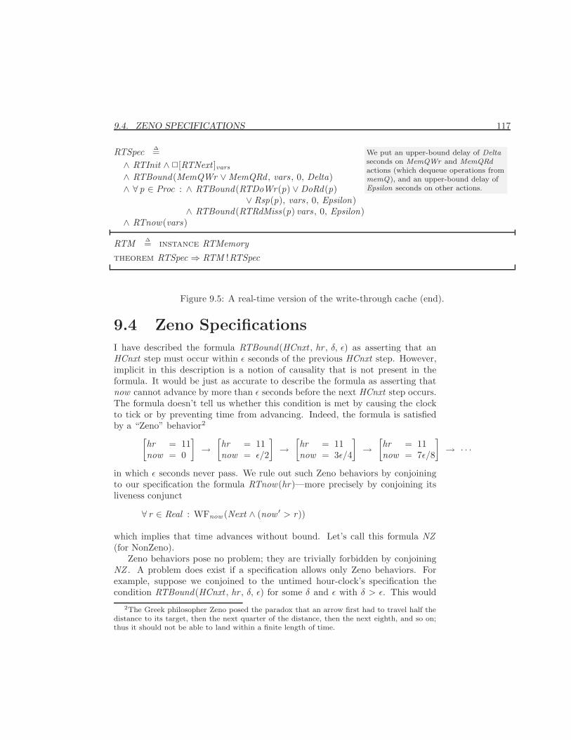
9.4. ZENO SPECIFICATIONS 117
RTSpec ∆=∧ RTInit ∧2[RTNext ]vars∧ RTBound(MemQWr ∨MemQRd , vars, 0, Delta)∧ ∀ p ∈ Proc : ∧ RTBound(RTDoWr(p) ∨DoRd(p)
∨ Rsp(p), vars, 0, Epsilon)∧ RTBound(RTRdMiss(p) vars, 0, Epsilon)
∧ RTnow(vars)
We put an upper-bound delay of Deltaseconds on MemQWr and MemQRdactions (which dequeue operations frommemQ), and an upper-bound delay ofEpsilon seconds on other actions.
RTM ∆= instance RTMemorytheorem RTSpec ⇒ RTM !RTSpec
Figure 9.5: A real-time version of the write-through cache (end).
9.4 Zeno Specifications
I have described the formula RTBound(HCnxt , hr , δ, ε) as asserting that anHCnxt step must occur within ε seconds of the previous HCnxt step. However,implicit in this description is a notion of causality that is not present in theformula. It would be just as accurate to describe the formula as asserting thatnow cannot advance by more than ε seconds before the next HCnxt step occurs.The formula doesn’t tell us whether this condition is met by causing the clockto tick or by preventing time from advancing. Indeed, the formula is satisfiedby a “Zeno” behavior2[
hr = 11now = 0
]→
[hr = 11now = ε/2
]→
[hr = 11now = 3ε/4
]→
[hr = 11now = 7ε/8
]→ · · ·
in which ε seconds never pass. We rule out such Zeno behaviors by conjoiningto our specification the formula RTnow(hr)—more precisely by conjoining itsliveness conjunct
∀ r ∈ Real : WFnow (Next ∧ (now ′ > r))
which implies that time advances without bound. Let’s call this formula NZ(for NonZeno).
Zeno behaviors pose no problem; they are trivially forbidden by conjoiningNZ . A problem does exist if a specification allows only Zeno behaviors. Forexample, suppose we conjoined to the untimed hour-clock’s specification thecondition RTBound(HCnxt , hr , δ, ε) for some δ and ε with δ > ε. This would
2The Greek philosopher Zeno posed the paradox that an arrow first had to travel half thedistance to its target, then the next quarter of the distance, then the next eighth, and so on;thus it should not be able to land within a finite length of time.
118 CHAPTER 9. REAL TIME
assert that the clock must wait at least δ seconds before ticking, but must tickwithin a shorter length of time. In other words, the clock could never tick. Onlya Zeno behavior, in which ε seconds never elapsed, can satisfy this specification.Conjoining NZ to this specification yields a formula that allows no behaviors—that is, a formula equivalent to false.
This example is an extreme case of what is called a Zeno specification. AZeno specification is one for which there exists a finite behavior σ that satisfiesthe safety part but cannot be extended to an infinite behavior that satisfies boththe safety part and NZ .3 In other words, the only complete behaviors satisfyingthe safety part that extend σ are Zeno behaviors. Equivalently, a specification isnonZeno iff the pair of properties consisting of the safety part of the specification(the conjunction of the untimed specification, the real-time bound conditions,and the safety part of the RTnow formula) and NZ is machine closed. Machine closed
specificationsare defined inSection 8.7.2 onpage 100.
A Zeno specification is one in which the requirement that time increaseswithout bound rules out some finite behaviors that would otherwise be allowed.Such a specification is likely to be incorrect because the real-time bound condi-tions are probably constraining the system in unintended ways. In this respect,Zeno specifications are much like other non-machine closed specifications.
In Section 8.7.2 I told you that the conjunction of fairness conditions onsubactions of the next-state relation produces a machine closed specification.There is an analogous result for real-time bound conditions and nonZeno spec-ifications. A specification is nonZeno if it is the conjunction of a formulaInit ∧ 2[Next ]vars , the formula RTnow(vars), and a finite number of formulasof the form RTBound(Ai , vars, δi , εi), where for each i :
• 0 ≤ δi ≤ εi ≤ Infinity
• Ai is a subaction of the next-state action Next .
• No step is both an Ai and an Aj step, for any Aj with j 6= i .
In particular, this implies that the specification RTSpec of the real-time write-through cache in module RTWriteThroughCache is nonZeno.
This result does not apply to the specification of the real-time memory inmodule RTMemory (Figure 9.3 on page 113) because the action Respond(p) isnot a subaction of the next-state action of formula ISpec. (Respond(p) can’tpossibly be a subaction of the next-state action because it doesn’t even mentionany of the specification’s variables except ctl .) The specification is nonethelessnonZeno, because any finite behavior σ that satisfies the specification can beextended to one in which time advances without bound. One can first extend σto respond to all pending requests immediately (in 0 time), and then extend itto a behavior performing nothing but clock ticks.
3Recall that a finite behavior σ satisfies a safety property P iff adding infinitely manystuttering steps to the end of σ produces a behavior that satisfies P .
9.5. HYBRID SYSTEM SPECIFICATIONS 119
It’s easy to construct an example in which conjoining an RTBound formulafor an action that is not a subaction of the next-state action produces a Zenospecification. For example, consider the formula
HC ∧ RTBound(hr ′ = hr − 1, hr , 0, 3600) ∧ RTNow(hr)(9.2)
where HC is the specification of the hour clock, whose next-state action HCnxtasserts that hr is either incremented by 1 or changes from 12 to 1. The RTBoundformula asserts that now cannot advance for 3600 or more seconds without anhr ′ = hr − 1 step occurring. Since HC asserts that every step that changes hris an HCnxt step, the safety part of (9.2) is satisfied only by behaviors in whichnow increases by less than 3600 seconds. Since the complete specification (9.2)contains the conjunct NZ , which asserts that now increases without bound, itis equivalent to false, and is thus a Zeno specification.
When a specification describes how a system is implemented, the real-timeconstraints are likely to be expressed as RTBound formulas for subactions ofthe next-state action. These are the kinds of formulas that correspond fairly di-rectly to an implementation. More abstract, higher-level specifications—onesdescribing what a system is supposed to do rather than how to do it—areless likely to have real-time constraints expressed in this ways. Thus, mod-ule RTWriteThroughCache describes an algorithm for implementing a memory,and it has real-time bounds on subactions of the next-state action. On the otherhand, the high-level specification of the real-time memory in module RTMemorycontains an RTBound formula for an action that is not a subaction of the next-state action.
9.5 Hybrid System Specifications
A system described by a TLA+ specification is a physical entity. The specifica-tion’s variables represent some part of the physical state—the display of a clock,or the distribution of charge in a piece of silicon that implements a memory cell.In a real-time specification, the variable now is different from the others becausewe are not abstracting away the continuous nature of time. The specificationallows now to assume any of a continuum of values. The discrete states in abehavior mean that we are observing the state of the system, and hence thevalue of now , at a sequence of discrete instants.
There may be physical quantities other than time whose continuous naturewe want to represent in a specification. For an air traffic control system, wemight want to represent the positions and velocities of the aircraft. For a systemcontrolling a nuclear reactor, we might want to represent the physical parametersof the reactor itself. A specification that represents such continually varyingquantities is called a hybrid system specification.
As an example, consider a system that, among other things, controls a switchthat influences the one-dimensional motion of some object. Suppose the object’s
120 CHAPTER 9. REAL TIME
position p obeys one of the following laws, depending on whether the switch isoff or on:
d2p/dt2+c∗dp/dt+f [t ] = 0 d2p/dt2+c∗dp/dt +f [t ]+k ∗p = 0(9.3)
where c and k are constants, f is some function, and t represents time. At anyinstant, the future position of the object is determined by the object’s currentposition and velocity. So, the state object is described by two variables—namely,its position p and its velocity w . These variables are related by related byw = dp/dt .
We describe this system with a TLA+ specification in which the variables pand w are changed only by steps that change now—that is, steps representingthe passage of time. We specify the changes to the discrete system state and anyreal-time constraints as before. However, we replace RTnow(v) with a formulahaving the following next-state action, where Integrate and D are explainedbelow:
∧ now ′ ∈ {r ∈ Real : r > now}∧ 〈p′,w ′ 〉 = Integrate(D ,now ,now ′, 〈p,w 〉)∧ unchanged v v is the tuple of all discrete variables, which change instantaneously.
The second conjunct asserts that p′ and w ′ equal the expressions obtained bysolving the appropriate differential equation for the object’s position and veloc-ity at time now ′, assuming that their values at time now are p and w . Thedifferential equation is specified by D , while Integrate is a general operator forsolving an arbitrary differential equation.
To specify the differential equation satisfied by the object, let’s suppose thatswitchOn is a Boolean-valued state variable that describes the position of theswitch. We can then rewrite the pair of equations (9.3) as
d2p/dt2 + c ∗ dp/dt + f [t ] + (if switchOn then −k ∗ p else 0) = 0
We the define the function D so this equation can be written as
D [t , p, dp/dt , d2p/dt2] = 0
Using the notation explained in Section 15.1.7 on page 275, the definition is:
D [t , p0, p1, p2 ∈ Real ] ∆= p2 + c ∗ p1 + f [t ] + (if switchOn then −k ∗ p else 0)
We obtain the desired specification if the operator Integrate is defined so thatIntegrate(D , t0, t1, 〈x 0, . . . , xn−1 〉) is the value at time t1 of the n-tuple
〈x , dx/dt , . . . , dn−1/dtn−1 〉where x is a solution to the differential equation
D [t , x , dx/dt , . . . , dnx/ctn ] = 0
9.6. REMARKS ON REAL TIME 121
whose 0th through (n−1)st derivatives at time t0 are x 0, . . . , xn−1. The defini-tion of Integrate appears in the DifferentialEquations module of Section 11.1.3.
In general, a hybrid-system specification is similar to a real-time specifica-tion, except that the formula RTNow(v) is replaced by one that describes thechanges to all variables that represent continuously changing physical quanti-ties. The Integrate operator will allow you to specify those changes for manyhybrid systems. Some systems will require different operators. For example,describing the evolution of some physical quantities might require an operatorfor describing the solution to a partial differential equation. However, if you candescribe the evolution mathematically, then it can be specified in TLA+.
Hybrid system specifications still seem to be of only academic interest, so Iwon’t say any more about them. If you do have occasion to write one, this briefdiscussion should indicate what you can do.
9.6 Remarks on Real Time
Real-time constraints are used most often to place an upper bound on how longit can take the system to do something. In this capacity, they can be considereda strong form of liveness, specifying not just that something must eventuallyhappen, but when it must happen. In very simple specifications, such as thehour clock and the write-through cache, real-time constraints usually replaceliveness conditions. More complicated specifications can assert both real-timeconstraints and liveness properties.
The real-time specifications I have seen have not required very complicatedtiming constraints. They have been specifications either of fairly simple algo-rithms in which timing constraints are crucial to correctness, or of more compli-cated systems in which real time appears only through the use of simple timeoutsto ensure liveness. I suspect that people don’t build systems with complicatedreal-time constraints because it’s too hard to get them right.
I’ve described how to write a real-time specification by conjoining RTnowand RTBound formulas to an untimed specification. One can prove that allreal-time specifications can be written in this form. In fact, it suffices to useRTBound formulas only for subactions of the next-state action. However, thisresult is of theoretical interest only because the resulting specification can beincredibly complicated. The operators RTnow and RTBound solve all the real-time specification problems that I have encountered; but I haven’t encounteredenough to say with confidence that they’re all you will ever need. Still, I amquite confident that whatever real-time properties you have to specify, it willnot be hard to express them in TLA+.

122 CHAPTER 9. REAL TIME
Chapter 10
Composing Specifications
Systems are usually described in terms of their components. In the specificationswe’ve written so far, the components have been represented as separate disjunctsof the next-state action. For example, the FIFO system pictured on page 35 isspecified in module InnerFIFO on page 38 by representing the three componentswith the following disjuncts of the next-state action:
Sender: ∃msg ∈ Message : SSend(msg)
Buffer: BufRcv ∨ BufSend
Receiver: RRcv
In this chapter, we learn how to specify the components separately and composetheir specifications to form a single system specification. Most of the time,there’s no point to doing this. The two ways of writing the specification differ byonly a few lines—a trivial difference in a specification of hundreds or thousandsof lines. Still, you may encounter a situation in which it’s better to specify asystem as a composition.
First, we must understand what it means to compose specifications. We usu-ally say that a TLA formula specifies the correct behavior of a system. However,as explained in Section 2.3 (page 18), a behavior actually represents a possiblehistory of the entire universe, not just of the system. So, it would be moreaccurate to say that a TLA formula specifies a universe in which the systembehaves correctly. Building a system that implements a specification F meansconstructing the universe so it satisfies F . (Fortunately, correctness of the sys-tem depends on the behavior of only a tiny part of the universe, so it’s justthat part that we must build.) Composing two systems whose specifications areF and G means making the universe satisfy both F and G, which is the sameas making it satisfy F ∧ G. Thus, the specification of the composition of twosystems is the conjunction of their specifications.
123
124 CHAPTER 10. COMPOSING SPECIFICATIONS
Writing a specification as the composition of its components therefore meanswriting the specification as a conjunction, each conjunct of which can be viewedas the specification of a component. While the basic idea is simple, the detailsare not always obvious. To simplify the exposition, I begin by considering onlysafety properties, ignoring liveness and largely ignoring hiding. Liveness andhiding are discussed in Section 10.6.
10.1 Composing Two Specifications
Let’s return once again to the simple hour clock, with no liveness or real-timerequirement. In Chapter 2, we specified such a clock whose display is representedby the variable hr . We can write that specification as
(hr ∈ 1 . . 12) ∧ 2[HCN (hr)]hr
where HCN is defined by:
HCN (h) ∆= h′ = (h % 12) + 1
Now let’s write a specification TwoClocks of a system composed of two separatehour clocks, whose displays are represented by the variables x and y. (The twoclocks are not synchronized and are completely independent of one another.) Wecan just define TwoClocks to be the conjunction of the two clock specifications:
TwoClocks ∆= ∧ (x ∈ 1 . . 12) ∧ 2[HCN (x )]x∧ (y ∈ 1 . . 12) ∧ 2[HCN (y)]y
The following calculation shows how we can rewrite TwoClocks in the usual formas a “monolithic” specification with a single next-state action:1
TwoClocks≡ ∧ (x ∈ 1 . . 12) ∧ (y ∈ 1 . . 12)∧ 2[HCN (x )]x ∧ 2[HCN (y)]y
≡ ∧ (x ∈ 1 . . 12) ∧ (y ∈ 1 . . 12)∧ 2 ( [HCN (x )]x ∧ [HCN (y)]y )
Because 2(F ∧ G) ≡ (2F ) ∧ (2G).
≡ ∧ (x ∈ 1 . . 12) ∧ (y ∈ 1 . . 12)∧ 2 (∧ HCN (x ) ∨ x ′ = x
∧ HCN (y) ∨ y ′ = y )
By definition of [. . .]x and [. . .]y .
1This calculation is informal because it contains formulas that are not legal TLA—namely,ones of the form 2A where A is an action that doesn’t have the syntactic form [B ]v . However,it can be done rigorously.
10.1. COMPOSING TWO SPECIFICATIONS 125
≡ ∧ (x ∈ 1 . . 12) ∧ (y ∈ 1 . . 12)∧ 2 (∨ HCN (x ) ∧ HCN (y)
∨ HCN (x ) ∧ (y ′ = y)∨ HCN (y) ∧ (x ′ = x )∨ (x ′ = x ) ∧ (y ′ = y) )
Because:∧ ∨ A1
∨ A2
∧ ∨ B1
∨ B2
≡
∨ A1 ∧ B1
∨ A1 ∧ B2
∨ A2 ∧ B1
∨ A2 ∧ B2
≡ ∧ (x ∈ 1 . . 12) ∧ (y ∈ 1 . . 12)∧ 2 [∨ HCN (x ) ∧ HCN (y)
∨ HCN (x ) ∧ (y ′ = y)∨ HCN (y) ∧ (x ′ = x ) ]〈x , y 〉
By definition of [. . .]〈x , y 〉.
Thus, TwoClocks is equivalent to Init ∧ 2[TCNxt ]〈x , y 〉 where the next-stateaction TCNxt is:
TCnxt ∆= ∨ HCN (x ) ∧HCN (y)∨ HCN (x ) ∧ (y ′ = y)∨ HCN (y) ∧ (x ′ = x )
This next-state action differs from the ones we are used to writing because of thedisjunct HCN (x ) ∧ HCN (y), which represents the simultaneous advance of thetwo displays. In the specifications we have written so far, different componentsnever act simultaneously.
Up until now, we have been writing what are called interleaving specifica-tions. In an interleaving specification, each step represents an operation of onlyone component. For example, in our FIFO specification, a (nonstuttering) steprepresents an action of either the sender, the buffer, or the receiver. For want of abetter term, we describe as noninterleaving a specification that, like TwoClocks,does permit simultaneous actions by two components.
Suppose we want to write an interleaving specification of the two-clock sys-tem as the conjunction of two component specifications. One way is to replacethe next-state actions HCN (x ) and HCN (y) of the two components by two ac-tions HCNx and HCNy so that, when we perform the analogous calculation tothe one above, we get
(∧ (x ∈ 1 . . 12) ∧ 2[HCNx ]x∧ (y ∈ 1 . . 12) ∧ 2[HCNy]y
)≡
∧ (x ∈ 1 . . 12) ∧ (y ∈ 1 . . 12)∧ 2 [∨ HCNx ∧ (y ′ = y)
∨ HCNy ∧ (x ′ = x ) ]〈x , y 〉
From the calculation above, we see that this equivalence holds if the followingthree conditions are satisfied: (i) HCNx implies HCN (x ), (ii) HCNy impliesHCN (y), and (iii) HCNx ∧ HCNy implies x ′ = x or y ′ = y. (Condition (iii)implies that the disjunct HCNx ∧ HCNy of the next-state relation is subsumedby one of the disjuncts HCNx ∧ (y ′ = y) and HCNy ∧ (x ′ = x ).) The common
126 CHAPTER 10. COMPOSING SPECIFICATIONS
way of satisfying these conditions is to let the next-state relation of each clockassert that the other clock’s display is unchanged. We do this by defining:
HCNx ∆= HCN (x ) ∧ (y ′ = y) HCNy ∆= HCN (y) ∧ (x ′ = x )
Another way to write an interleaving specification is simply to disallow si-multaneous changes to both clock displays. We can do this by taking as ourspecification the formula:
TwoClocks ∧ 2[(x ′ = x ) ∨ (y ′ = y)]〈x , y 〉
The second conjunct asserts that any step must leave x or y (or both) unchanged.Everything we have done for the two-clock system generalizes to any system
comprising two components. The same calculation as above shows that if
(v1′ = v1) ∧ (v2
′ = v2) ≡ (v ′ = v) This asserts that v is unchanged iff both v1 and v2 are.
then
(∧ I1 ∧ 2[N1]v1
∧ I2 ∧ 2[N2]v2
)≡
∧ I1 ∧ I2
∧ 2 [∨ N1 ∧N2
∨ N1 ∧ (v2′ = v2)
∨ N2 ∧ (v1′ = v1) ]v
(10.1)
for any state predicates I1 and I2 and any actions N1 and N2. The left-hand sideof this equivalence represents the composition of two component specificationsif vk is a tuple containing the variables that describe the k th component, fork = 1, 2, and v is the tuple of all the variables.
The equivalent formulas in (10.1) represent an interleaving specification ifthe first disjunct in the next-state action of the right-hand side is redundant, soit can be removed. This is the case if N1∧N2 implies that v1 or v2 is unchanged.The usual way to ensure that this condition is satisfied is by defining each Nk
so it implies that the other component’s tuple is left unchanged. Another wayto obtain an interleaving specification by conjoining the formula 2[(v1
′ = v1) ∨(v2′ = v2)]v .
10.2 Composing Many Specifications
We can generalize (10.1) to the composition of any set C of components. Be-cause universal quantification generalizes conjunction, the following rule is ageneralization of (10.1):
Composition Rule For any set C , if
(∀ k ∈ C : vk′ = vk) ≡ (v ′ = v) This asserts that v is unchanged iff all the vk are.
10.2. COMPOSING MANY SPECIFICATIONS 127
then
(∀ k ∈ C : Ik ∧ 2[Nk]vk) ≡
∧ ∀ k ∈ C : Ik
∧ 2[∨ ∃ k ∈ C : Nk ∧ (∀ i ∈ C \ {k} : vi
′ = vi)∨ ∀ i , j ∈ C : (i 6= j ) ∧Ni ∧Nj ∧ F ij
]v
for some action Fij .
The disjunct containing Fij is redundant, and we have an interleaving speci-fication, if Ni ∧ Nj implies that vi or vj is unchanged, for all i and j in Cwith i 6= j . Typically, this is made true by letting each Nk imply that vj is un-changed for all j in C other than k . However, that means that Nk must mentionvj for components j other than k . You might object to this approach—either onphilosophical grounds, because you feel that the specification of one componentshould not mention the state of another component, or because mentioning othercomponent’s variables complicates the component’s specification. An alterna-tive approach is simply to assert interleaving. You can do this by conjoining thefollowing formula, which states that no step changes both vi and vj , for any iand j with i 6= j :
2 [ ∃ k ∈ C : ∀ i ∈ C \ {k} : vi′ = vi ]v
This conjunct can be viewed as a global condition, not attached to any compo-nent’s specification.
For the left-hand side of the conclusion of the Composition Rule to representthe composition of separate components, the vk need not be composed of sep-arate variables. They could contain different “parts” of the same variable thatdescribe different components. For example, our system might consist of a setClock of separate, independent clocks, where clock k ’s display is described bythe value of hr [k ]. Then vk would equal hr [k ]. It’s easy to specify such an arrayof clocks as a composition. Using the definition of HCN on page 124 above, wecan write the specification as:
ClockArray ∆= ∀ k ∈ Clock : (hr [k ] ∈ 1 . . 12) ∧ 2[HCN (hr [k ])]hr [k ](10.2)
This is a noninterleaving specification, since it allows simultaneous steps bydifferent clocks.
Suppose we wanted to use the Composition Rule to express ClockArray asa monolithic specification. What would we substitute for v? Our first thoughtis to substitute hr for v . However, the hypothesis of the rule requires that vmust be left unchanged iff hr [k ] is left unchanged, for all k ∈ Clock . However,as explained in Section 6.5 on page 71, specifying the values of hr [k ]′ for all
128 CHAPTER 10. COMPOSING SPECIFICATIONS
k ∈ Clock does not specify the value of hr . It doesn’t even imply that hr is afunction. We must substitute for v the function hrfcn defined by
hrfcn ∆= [k ∈ Clock 7→ hr [k ]](10.3)
This function equals hr iff hr is a function with domain Clock . Formula ClockArraydoes not imply that hr is always a function. It specifies the possible values ofhr [k ], for all k ∈ Clock , but it does not specify the value of hr . Even if wechanged the initial condition to imply that hr is initially a function with do-main Clock , formula ClockArray allows arbitrary steps that leave each hr [k ]unchanged, but which can change hr in unknown ways.
We might prefer to write a specification in which hr is a function with domainClock . (For example, some tool might require that the value of hr be completelyspecified.) One way of doing this is to conjoin to the specification the formula2IsFcnOn(hr , Clock), where IsFcnOn(hr , Clock) asserts that hr is an arbitraryfunction with domain Clock . The operator IsFcnOn is defined by
IsFcnOn(f , S ) ∆= f = [x ∈ S 7→ f [x ]]
We can view the formula 2IsFcnOn(hr , Clock) as a global constraint on hr ,while the value of hr [k ] for each component k is described by that component’sspecification.
Now suppose we want to write an interleaving specification of the arrayof clocks, again as the composition of specifications of the individual clocks.In general, for the conjunction in the Composition Rule to be an interleavingspecification, Ni ∧Nj should imply that vi or vj is unchanged. We can do thisby letting the next-state relation Nk of clock k imply that hr [i ] is unchangedfor every clock i other than k . The most obvious way to do this is to define Nk
to equal:
∧ hr ′[k ] = (hr [k ] % 12) + 1∧ ∀ i ∈ Clock \ {k} : hr ′[i ] = hr [i ]
We can express this formula more compactly using the except construct. This The except con-struct is explainedin Section 5.2 onpage 48.
construct applies only to functions, so we must choose whether or not to requirehr to be a function. If hr is a function, then we can let Nk equal
hr ′ = [hr except ! [k ] = (hr [k ] % 12) + 1](10.4)
As noted above, we can ensure that hr is a function by conjoining the formula2IsFcnOn(hr , Clock) to the specification. Another way is to define the statefunction hrfcn by (10.3) on this page and let N (k) equal
hrFcn ′ = [hrFcn except ! [k ] = (hr [k ] % 12) + 1]
As we’ve seen before, a specification is just a mathematical formula, and thereare often many equivalent ways to write a formula. Which one you choose isusually a matter of taste.
10.3. THE FIFO 129
10.3 The FIFO
Let’s now specify the FIFO, described in Chapter 4, as the composition of itsthree components—the Sender, the Buffer, and the Receiver. We start with theinternal specification, in which the variable q occurs—that is, q is not hidden.First, we decide what part of the state describes each component. The variablesin and out are channels. Recall that the Channel module (page 30) specifiesa channel chan to be a record with val , rdy, and ack components. The Sendaction, which sends a value, modifies the val and rdy components; the Rcvaction, which receives a value, modifies the ack component. So, the components’states are described by the following state functions:
Sender: 〈in.val , in.rdy 〉Buffer: 〈in.ack , q, out .val , out .rdy 〉Receiver: out .ack
Unfortunately, we can’t reuse the definitions from the InnerFIFO module onpage 38 for the following reason. The variable q, which is hidden in the finalspecification, is part of the Buffer component’s internal state. Therefore, itshould not appear in the specifications of the Sender or Receiver component.The Sender and Receiver actions defined in the InnerFIFO module all mention q,so we can’t use them. We therefore won’t bother reusing that module. However,instead of starting completely from scratch, we can make use of the of the Sendand Rcv actions from the Channel module on page 30 to describe the changesto in and out .
Let’s write a noninterleaving specification. The next-state actions of thecomponents are then the same as the corresponding disjuncts of the Next ac-tion in module InnerFIFO , except that they do not mention the parts of thestates belonging to the other components. These contain Send and Rcv actions,instantiated from the Channel module, which use the except construct. Asnoted above, we can apply except only to functions—and to records, which are Section 5.2 on
page 48 explainswhy records arefunctions.
functions. We therefore add to our specification the conjunct
2(IsChannel(in) ∧ IsChannel(out))
where IsChannel(c) asserts that c is a channel—that is a record with val ,ack , and rdy fields. Since a record with val , ack , and rdy fields is a func-tion whose domain is {“val”, “ack”, “rdy”}, we can define IsChannel(c) to equalIsFcnOn(c, {“val”, “ack”, “rdy”}). However, it’s just as easy to define IsChannel(c)directly by
IsChannel(c) ∆= c = [ack 7→ c.ack , val 7→ c.val , rdy 7→ c.rdy]
In writing this specification, we face the same problem as in our original FIFOspecification of introducing the variable q and then hiding it. In Chapter 4, we
130 CHAPTER 10. COMPOSING SPECIFICATIONS
solved this problem by introducing q in a separate InnerFIFO module, whichis instantiated by the FIFO module that defines the final specification. Wedo essentially the same thing here, except that we introduce q in a submoduleinstead of in a completely separate module. All the symbols declared and definedat the point where the submodule appears can be used within it. The submoduleitself can be instantiated in the containing module anywhere after it appears.(Submodules are used in the RealTimeHourClock and RTMemory specificationson pages 109 and 113 of Chapter 9.)
There is one small problem to be solved before we can write a compositespecification of the FIFO—how to specify the initial predicates. It makes sensefor the initial predicate of each component’s specification to specify the initialvalues of its part of the state. However the initial condition includes the require-ments in.ack = in.rdy and out .ack = out .rdy, each of which relates the initialstates of two different components. (These requirements are stated in moduleInnerFIFO by the conjuncts InChan !Init and OutChan !Init of the initial pred-icate Init .) There are three ways of expressing a requirement that relates theinitial states of multiple components:
• Assert it in the initial conditions of all the components. Although sym-metric, this seems needlessly redundant.
• Arbitrarily assign the requirement to one of the components. This intu-itively suggests that we are assigning to that component the responsibilityof ensuring that the requirement is met.
• Assert the requirement as a conjunct separate from either of the componentspecifications. This intuitively suggests that it is an assumption abouthow the components are put together, rather than a requirement of eithercomponent.
When we write an open-system specification, as described in Section 10.7 below,the intuitive suggestions of the last two approaches can be turned into formalrequirements. I’ve taken the last approach and added
(in.ack = in.rdy) ∧ (out .ack = out .rdy)
as a separate condition. The complete specification is in module CompositeFIFOof Figure 10.1 on the next page. Formula Spec of this module is a noninterleavingspecification; for example, it allows a single step that is both an InChan !Sendstep (the sender sends a value and an OutChan !Rcv step (the receiver acknowl-edges a value). Hence, it is not equivalent to the interleaving specification Specof the FIFO module on page 41, which does not allow such a step.
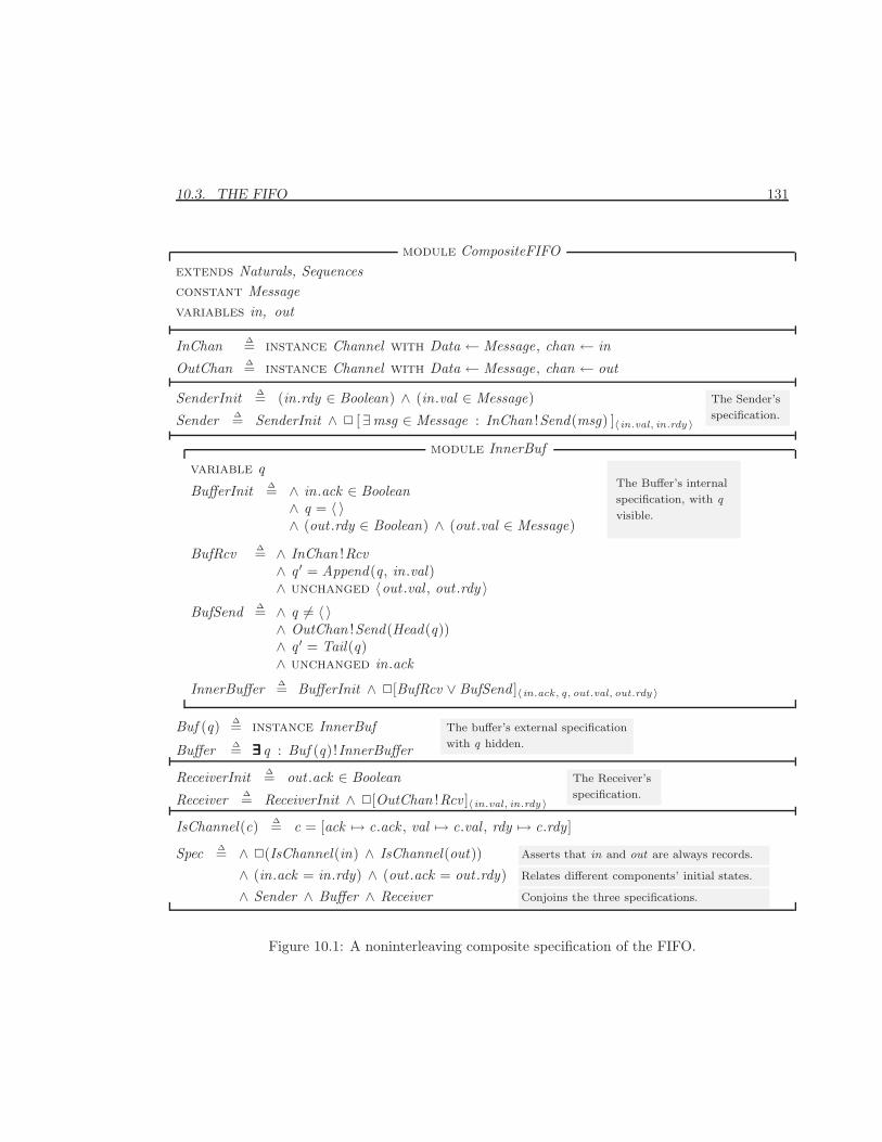
10.3. THE FIFO 131
module CompositeFIFOextends Naturals, Sequencesconstant Messagevariables in, out
InChan ∆= instance Channel with Data ← Message, chan ← in
OutChan ∆= instance Channel with Data ← Message, chan ← out
SenderInit ∆= (in.rdy ∈ Boolean) ∧ (in.val ∈ Message)
Sender ∆= SenderInit ∧ 2 [ ∃msg ∈ Message : InChan !Send(msg) ]〈in.val, in.rdy 〉
The Sender’s
specification.
module InnerBufvariable q
BufferInit ∆= ∧ in.ack ∈ Boolean∧ q = 〈 〉∧ (out .rdy ∈ Boolean) ∧ (out .val ∈ Message)
The Buffer’s internal
specification, with q
visible.
BufRcv ∆= ∧ InChan !Rcv∧ q ′ = Append(q, in.val)∧ unchanged 〈out .val , out .rdy 〉
BufSend ∆= ∧ q 6= 〈 〉∧ OutChan !Send(Head(q))∧ q ′ = Tail(q)∧ unchanged in.ack
InnerBuffer ∆= BufferInit ∧ 2[BufRcv ∨ BufSend ]〈in.ack , q, out.val, out.rdy 〉
Buf (q) ∆= instance InnerBuf
Buffer ∆= ∃∃∃∃∃∃ q : Buf (q)!InnerBuffer
The buffer’s external specification
with q hidden.
ReceiverInit ∆= out .ack ∈ Boolean
Receiver ∆= ReceiverInit ∧ 2[OutChan !Rcv ]〈in.val, in.rdy 〉
The Receiver’s
specification.
IsChannel(c) ∆= c = [ack 7→ c.ack , val 7→ c.val , rdy 7→ c.rdy]
Spec ∆= ∧ 2(IsChannel(in) ∧ IsChannel(out))∧ (in.ack = in.rdy) ∧ (out .ack = out .rdy)∧ Sender ∧ Buffer ∧ Receiver
Asserts that in and out are always records.
Relates different components’ initial states.
Conjoins the three specifications.
Figure 10.1: A noninterleaving composite specification of the FIFO.
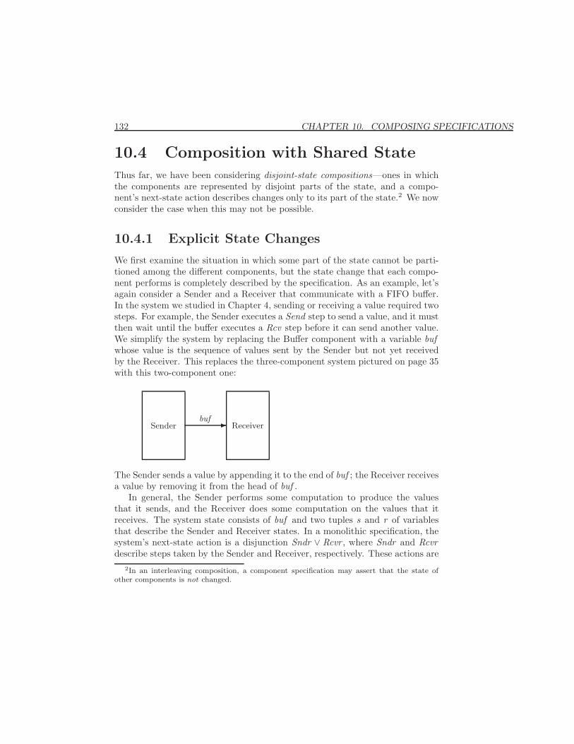
132 CHAPTER 10. COMPOSING SPECIFICATIONS
10.4 Composition with Shared State
Thus far, we have been considering disjoint-state compositions—ones in whichthe components are represented by disjoint parts of the state, and a compo-nent’s next-state action describes changes only to its part of the state.2 We nowconsider the case when this may not be possible.
10.4.1 Explicit State Changes
We first examine the situation in which some part of the state cannot be parti-tioned among the different components, but the state change that each compo-nent performs is completely described by the specification. As an example, let’sagain consider a Sender and a Receiver that communicate with a FIFO buffer.In the system we studied in Chapter 4, sending or receiving a value required twosteps. For example, the Sender executes a Send step to send a value, and it mustthen wait until the buffer executes a Rcv step before it can send another value.We simplify the system by replacing the Buffer component with a variable bufwhose value is the sequence of values sent by the Sender but not yet receivedby the Receiver. This replaces the three-component system pictured on page 35with this two-component one:
Sender Receiverbuf -
The Sender sends a value by appending it to the end of buf ; the Receiver receivesa value by removing it from the head of buf .
In general, the Sender performs some computation to produce the valuesthat it sends, and the Receiver does some computation on the values that itreceives. The system state consists of buf and two tuples s and r of variablesthat describe the Sender and Receiver states. In a monolithic specification, thesystem’s next-state action is a disjunction Sndr ∨ Rcvr , where Sndr and Rcvrdescribe steps taken by the Sender and Receiver, respectively. These actions are
2In an interleaving composition, a component specification may assert that the state ofother components is not changed.
10.4. COMPOSITION WITH SHARED STATE 133
defined by
Sndr ∆= ∨ ∧ buf ′ = Append(buf , . . .)∧ SComm∧ unchanged r∨ ∧ SCompute∧ unchanged 〈buf , r 〉
Rcvr ∆= ∨ ∧ buf 6= 〈 〉∧ buf ′ = Tail(buf )∧ RComm∧ unchanged s∨ ∧ RCompute∧ unchanged 〈buf , s 〉
for some actions SComm, SCompute, RComm, and RCompute. For simplicity,we assume that neither Sndr nor Rcvr allows stuttering actions, so SComputechanges s and RCompute changes r . We now write the specification as thecomposition of separate specifications of the Sender and Receiver.
Splitting the initial predicate is straightforward. The initial conditions ons belong to the Sender’s initial predicate; those on r belong to the Receiver’sinitial predicate; and the initial condition buf = 〈 〉 can be assigned arbitrarilyto either of them.
Now let’s consider the next-state actions NS and NR of the Sender andReceiver components. The trick is to define them by
NS ∆= Sndr ∨ (σ ∧ (s ′ = s)) NR ∆= Rcvr ∨ (ρ ∧ (r ′ = r))
where σ and ρ are actions containing only the variable buf . Think of σ asdescribing possible changes to buf that are not caused by the Sender, and ρ asdescribing possible changes to buf that are not caused by the Receiver. Thus,NS permits any step that is either a Sndr step or one that leaves s unchangedand is a change to buf that can’t be “blamed” on the Sender.
Suppose σ and ρ satisfy the following three conditions:
• ∀ d : (buf ′ = Append(buf , d))⇒ ρA step that appends a value to buf is not caused by the Receiver.
• (buf 6= 〈 〉) ∧ (buf ′ = Tail(buf ))⇒ σA step that removes a value from the head of buf is not caused by theSender.
• (σ ∧ ρ)⇒ (buf ′ = buf )A step that is caused by neither the Sender nor the Receiver cannot changebuf .
Using the relation3
(buf ′ = Append(buf , . . .)) ∧ (buf 6= 〈 〉) ∧ (buf ′ = Tail(buf )) ≡ false
3This relation is valid only if buf is a sequence. A rigorous calculation requires the use ofan invariant to assert that buf is indeed a sequence.
134 CHAPTER 10. COMPOSING SPECIFICATIONS
a computation like the one by which we derived (10.1) shows
2[NS ]〈buf , s 〉 ∧ 2[NR]〈buf , r 〉 ≡ 2[Sndr ∨ Rcvr ]〈buf , s, r 〉
Thus, NS and NR are suitable next-state relations for the components, if wechoose σ and ρ to satisfy the three conditions above. There is considerablefreedom in that choice. The strongest possible choices of σ and ρ are ones thatdescribe exactly the changes permitted by the other component:
σ∆= (buf 6= 〈 〉) ∧ (buf ′ = Tail(buf ))
ρ∆= ∃ d : buf ′ = Append(buf , d)
We can weaken these definitions any way we want, so long as we maintain thecondition that σ ∧ ρ implies that buf is unchanged. For example, we can defineσ as above and let ρ equal ¬σ. The choice is a matter of taste.
I’ve been describing an interleaving specification of the Sender/Receiver sys-tem. Now let’s consider a noninterleaving specification—one that allows stepsin which both the Sender and the Receiver are computing. In other words, wewant the specification to allow SCompute ∧RCompute steps that leave buf un-changed. Let SSndr be the action that is the same as Sndr except it doesn’tmention r , and let RRcvr be defined analogously. Then we have:
Sndr ≡ SSndr ∧ (r ′ = r) Rcvr ≡ RRcvr ∧ (s ′ = s)
A monolithic noninterleaving specification has the next-state relation
Sndr ∨ Rcvr ∨ (SSndr ∧ SRcvr ∧ (buf ′ = buf ))
It is the conjunction of component specifications having the next-state relationsNS and NR defined by
NS ∆= SSndr ∨ (σ ∧ (s ′ = s)) NR ∆= RRcvr ∨ (ρ ∧ (r ′ = r))
where σ and ρ are as above.This two-process situation generalizes to the composition of any set C of
components that share a variable or tuple of variables w . The interleavingcase generalizes to the following rule, in which Nk is the next-state action ofcomponent k , the action µk describes all changes to w that are attributed tosome component other than k , the tuple vk describes the private state of k , andv is the tuple formed by all the vk.
Shared-State Composition Rule The four conditions
1. (∀ k ∈ C : vk′ = vk) ≡ (v ′ = v)
v is unchanged iff the private state vk of every component is unchanged.
2. ∀ i , k ∈ C : Nk ∧ (i 6= k)⇒ (vi′ = vi)
The next-state action of any component k leaves the private state vi of allother components i unchanged.
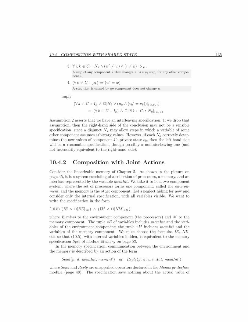
10.4. COMPOSITION WITH SHARED STATE 135
3. ∀ i , k ∈ C : Nk ∧ (w ′ 6= w) ∧ (i 6= k)⇒ µi
A step of any component k that changes w is a µi step, for any other compo-nent i .
4. (∀ k ∈ C : µk)⇒ (w ′ = w)A step that is caused by no component does not change w .
imply
(∀ k ∈ C : Ik ∧ 2[Nk ∨ (µk ∧ (vk′ = vk))]〈w,vk 〉)
≡ (∀ k ∈ C : Ik) ∧ 2 [∃ k ∈ C : Nk]〈w, v 〉
Assumption 2 asserts that we have an interleaving specification. If we drop thatassumption, then the right-hand side of the conclusion may not be a sensiblespecification, since a disjunct Nk may allow steps in which a variable of someother component assumes arbitrary values. However, if each Nk correctly deter-mines the new values of component k ’s private state vk, then the left-hand sidewill be a reasonable specification, though possibly a noninterleaving one (andnot necessarily equivalent to the right-hand side).
10.4.2 Composition with Joint Actions
Consider the linearizable memory of Chapter 5. As shown in the picture onpage 45, it is a system consisting of a collection of processors, a memory, and aninterface represented by the variable memInt . We take it to be a two-componentsystem, where the set of processors forms one component, called the environ-ment, and the memory is the other component. Let’s neglect hiding for now andconsider only the internal specification, with all variables visible. We want towrite the specification in the form
(IE ∧ 2[NE ]vE ) ∧ (IM ∧ 2[NM ]vM )(10.5)
where E refers to the environment component (the processors) and M to thememory component. The tuple vE of variables includes memInt and the vari-ables of the environment component; the tuple vM includes memInt and thevariables of the memory component. We must choose the formulas IE , NE ,etc. so that (10.5), with internal variables hidden, is equivalent to the memoryspecification Spec of module Memory on page 53.
In the memory specification, communication between the environment andthe memory is described by an action of the form
Send(p, d , memInt , memInt ′) or Reply(p, d , memInt , memInt ′)
where Send and Reply are unspecified operators declared in the MemoryInterfacemodule (page 48). The specification says nothing about the actual value of
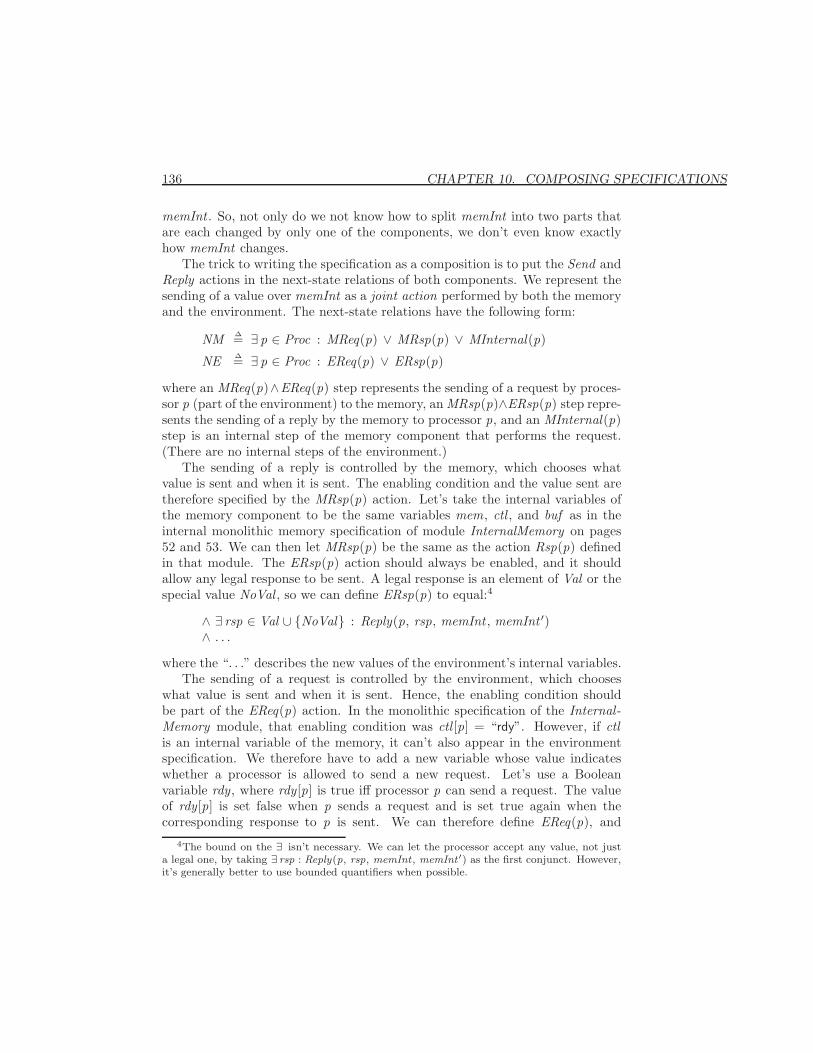
136 CHAPTER 10. COMPOSING SPECIFICATIONS
memInt . So, not only do we not know how to split memInt into two parts thatare each changed by only one of the components, we don’t even know exactlyhow memInt changes.
The trick to writing the specification as a composition is to put the Send andReply actions in the next-state relations of both components. We represent thesending of a value over memInt as a joint action performed by both the memoryand the environment. The next-state relations have the following form:
NM ∆= ∃ p ∈ Proc : MReq(p) ∨ MRsp(p) ∨ MInternal(p)
NE ∆= ∃ p ∈ Proc : EReq(p) ∨ ERsp(p)
where an MReq(p)∧EReq(p) step represents the sending of a request by proces-sor p (part of the environment) to the memory, an MRsp(p)∧ERsp(p) step repre-sents the sending of a reply by the memory to processor p, and an MInternal(p)step is an internal step of the memory component that performs the request.(There are no internal steps of the environment.)
The sending of a reply is controlled by the memory, which chooses whatvalue is sent and when it is sent. The enabling condition and the value sent aretherefore specified by the MRsp(p) action. Let’s take the internal variables ofthe memory component to be the same variables mem, ctl , and buf as in theinternal monolithic memory specification of module InternalMemory on pages52 and 53. We can then let MRsp(p) be the same as the action Rsp(p) definedin that module. The ERsp(p) action should always be enabled, and it shouldallow any legal response to be sent. A legal response is an element of Val or thespecial value NoVal , so we can define ERsp(p) to equal:4
∧ ∃ rsp ∈ Val ∪ {NoVal} : Reply(p, rsp, memInt , memInt ′)∧ . . .
where the “. . .” describes the new values of the environment’s internal variables.The sending of a request is controlled by the environment, which chooses
what value is sent and when it is sent. Hence, the enabling condition shouldbe part of the EReq(p) action. In the monolithic specification of the Internal -Memory module, that enabling condition was ctl [p] = “rdy”. However, if ctlis an internal variable of the memory, it can’t also appear in the environmentspecification. We therefore have to add a new variable whose value indicateswhether a processor is allowed to send a new request. Let’s use a Booleanvariable rdy, where rdy[p] is true iff processor p can send a request. The valueof rdy[p] is set false when p sends a request and is set true again when thecorresponding response to p is sent. We can therefore define EReq(p), and
4The bound on the ∃ isn’t necessary. We can let the processor accept any value, not justa legal one, by taking ∃ rsp : Reply(p, rsp, memInt , memInt ′) as the first conjunct. However,it’s generally better to use bounded quantifiers when possible.
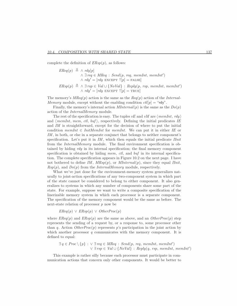
10.4. COMPOSITION WITH SHARED STATE 137
complete the definition of ERsp(p), as follows:
EReq(p) ∆= ∧ rdy[p]∧ ∃ req ∈ MReq : Send(p, req, memInt , memInt ′)∧ rdy ′ = [rdy except ! [p] = false]
ERsp(p) ∆= ∧ ∃ rsp ∈ Val ∪ {NoVal} : Reply(p, rsp, memInt , memInt ′)∧ rdy ′ = [rdy except ! [p] = true]
The memory’s MReq(p) action is the same as the Req(p) action of the Internal -Memory module, except without the enabling condition ctl [p] = “rdy”.
Finally, the memory’s internal action MInternal(p) is the same as the Do(p)action of the InternalMemory module.
The rest of the specification is easy. The tuples vE and vM are 〈memInt , rdy 〉and 〈memInt , mem, ctl , buf 〉, respectively. Defining the initial predicates IEand IM is straightforward, except for the decision of where to put the initialcondition memInt ∈ InitMemInt for memInt . We can put it in either IE orIM , in both, or else in a separate conjunct that belongs to neither component’sspecification. Let’s put it in IM , which then equals the initial predicate IInitfrom the InternalMemory module. The final environment specification is ob-tained by hiding rdy in its internal specification; the final memory componentspecification is obtained by hiding mem, ctl , and buf in its internal specifica-tion. The complete specification appears in Figure 10.2 on the next page. I havenot bothered to define IM , MRsp(p), or MInternal(p), since they equal IInit ,Rsp(p), and Do(p) from the InternalMemory module, respectively.
What we’ve just done for the environment-memory system generalizes nat-urally to joint-action specifications of any two-component system in which partof the state cannot be considered to belong to either component. It also gen-eralizes to systems in which any number of components share some part of thestate. For example, suppose we want to write a composite specification of thelinerizable memory system in which each processor is a separate component.The specification of the memory component would be the same as before. Thenext-state relation of processor p now be
EReq(p) ∨ ERsp(p) ∨ OtherProc(p)
where EReq(p) and ERsp(p) are the same as above, and an OtherProc(p) steprepresents the sending of a request by, or a response to, some processor otherthan q. Action OtherProc(p) represents p’s participation in the joint action bywhich another processor q communicates with the memory component. It isdefined to equal:
∃ q ∈ Proc \ {p} : ∨ ∃ req ∈ MReq : Send(p, req, memInt , memInt ′)∨ ∃ rsp ∈ Val ∪ {NoVal} : Reply(q, rsp, memInt , memInt ′)
This example is rather silly because each processor must participate in com-munication actions that concern only other components. It would be better to
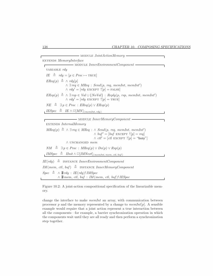
138 CHAPTER 10. COMPOSING SPECIFICATIONS
module JointActionMemoryextends MemoryInterface
module InnerEnvironmentComponentvariable rdy
IE ∆= rdy = [p ∈ Proc 7→ true]
EReq(p) ∆= ∧ rdy[p]∧ ∃ req ∈ MReq : Send(p, req, memInt , memInt ′)∧ rdy ′ = [rdy except ! [p] = false]
ERsp(p) ∆= ∧ ∃ rsp ∈ Val ∪ {NoVal} : Reply(p, rsp, memInt , memInt ′)∧ rdy ′ = [rdy except ! [p] = true]
NE ∆= ∃ p ∈ Proc : EReq(p) ∨ ERsp(p)
IESpec ∆= IE ∧2[MN ]〈memInt, rdy 〉
module InnerMemoryComponentextends InternalMemory
MReq(p) ∆= ∧ ∃ req ∈ MReq : ∧ Send(p, req, memInt , memInt ′)∧ buf ′ = [buf except ! [p] = req]∧ ctl ′ = [ctl except ! [p] = “busy”]
∧ unchanged mem
NM ∆= ∃ p ∈ Proc : MReq(p) ∨Do(p) ∨Rsp(p)
IMSpec ∆= IInit ∧ 2[IMNext ]〈memInt,mem, ctl, buf 〉
IE(rdy) ∆= instance InnerEnvironmentComponent
IM (mem, ctl , buf ) ∆= instance InnerMemoryComponent
Spec ∆= ∧ ∃∃∃∃∃∃ rdy : IE(rdy)!IMSpec∧ ∃∃∃∃∃∃mem, ctl , buf : IM (mem, ctl , buf )!IESpec
Figure 10.2: A joint-action compositional specification of the linearizable mem-ory.
change the interface to make memInt an array, with communication betweenprocessor p and the memory represented by a change to memInt [p]. A sensibleexample would require that a joint action represent a true interaction betweenall the components—for example, a barrier synchronization operation in whichthe components wait until they are all ready and then perform a synchronizationstep together.
10.5. A BRIEF REVIEW 139
10.5 A Brief Review
The basic idea of composing specifications is simple: a composite specificationis the conjunction of formulas, each of which can be considered to be the specifi-cation of a separate component. I have presented several techniques for writinga specification as a composition. Before going further, let’s put these techniquesin perspective.
10.5.1 A Taxonomy of Composition
I have introduced three different ways of categorizing composite specifications:
Interleaving versus noninterleaving. An interleaving specification is one inwhich each (nonstuttering) step can be attributed to exactly one compo-nent. A noninterleaving specification allows steps that represent simulta-neous operations of two or more different components.
Disjoint-state versus shared-state. A disjoint-state specification is one inwhich the state can be partitioned, with each part belonging to a separatecomponent. A part of the state can be a variable v , or a “piece” of thatvariable such as v .c or v [c] for some fixed c. Any change to a component’spart of the state is attributed to that component. In a shared-state speci-fication, some part of the state can be changed by steps attributed to morethan one component.
Joint-action versus separate-action. A joint-action specification is a nonin-terleaving one in which some step attributed to one component must occursimultaneously with a step attributed to another component. A separate-action specification is simply one that is not a joint-action specification.
These categories are orthogonal, except that a joint-action specification must benoninterleaving.
10.5.2 Interleaving Reconsidered
Should we write interleaving or noninterleaving specifications? We might try toanswer this question by asking, can different components really take simultane-ous steps? However, this question makes no sense. A step is a mathematicalabstraction; real components perform operations that take a finite amount oftime. Operations performed by two different components could overlap in time.We are free to represent this physical situation either with a single simultaneousstep of the two components, or with two separate steps. In the latter case, thespecification usually allows the two steps to occur in either order. (If the two
140 CHAPTER 10. COMPOSING SPECIFICATIONS
operations must occur simultaneously, then we have written a joint-action spec-ification.) It’s up to you whether to write an interleaving or a noninterleavingspecification. You should choose whichever is more convenient.
The choice is not completely arbitrary if you want one specification to imple-ment another. A noninterleaving specification will not, in general, implement aninterleaving one because the noninterleaving specification will allow simultane-ous actions that the interleaving specification prohibits. So, if you want to writea low-level specification that implements a high-level interleaving specification,then you’ll have to use an interleaving specification. As we’ve seen, it’s easy toturn a noninterleaving specification into an interleaving one by conjoining aninterleaving assumption.
10.5.3 Joint Actions Reconsidered
The reason for writing a composite specification is to separate the specificationsof the different components. The mixing of actions from different componentsin a joint-action specification destroys this separation. So, why should we writesuch a specification?
Joint-action specifications arise most often in highly abstract descriptions ofinter-component communication. In writing a composite specification of the lin-earizable memory, we were led to use joint actions because of the abstract natureof the interface. In real systems, communication occurs when one componentchanges the state and another component later observes that change. The inter-face described by the MemoryInterface module abstracts away those two steps,replacing them with a single one that represents instantaneous communication—a fiction that does not exist in the real world. Since each component must re-member that the communication has occurred, the single communication stephas to change the private state of both components. That’s why we couldn’tuse the approach of Section 10.4.1, which requires that any change to the sharedinterface change the nonshared state of just one component.
The abstract memory interface simplifies the specification, allowing commu-nication to be represented as one step instead of two. But this simplificationcomes at the cost of blurring the distinction between the two components. If weblur this distinction, it may not make sense to write the specification as the con-junction of separate component specifications. As the memory system exampleillustrates, decomposing the system into separate components communicatingwith joint actions may require the introduction of extra variables. There mayoccasionally be a good reason for adding this kind of complexity to a specifica-tion, but it should not be done as a matter of course.
10.6. LIVENESS AND HIDING 141
10.6 Liveness and Hiding
10.6.1 Liveness and Machine Closure
Thus far, the discussion of composition has neglected liveness. In compositespecifications, it is usually easy to specifying liveness by placing fairness con-ditions on the actions of individual components. For example, to specify anarray of clocks that all keep ticking forever, we would modify the specificationClockArray of (10.2) on page 127 to equal:
∀ k ∈ Clock : (hr [k ] ∈ 1 . . 12) ∧ 2[HCN (hr [k ])]hr [k ] ∧ WFhr [k ](HCN (hr [k ]))
When writing a weak or strong fairness formula for an action A of componentc, there arises the question of what the subscript should be. The obvious choicesare (i) the tuple v describing the entire specification state, and (ii) the tuple vc
describing that component’s state.5 The choice matters only if the safety partof the specification allows the system to reach some state in which an A stepcould leave vc unchanged while changing v . In practice, this is seldom the case.If it is, we probably don’t want the fairness condition to be satisfied by a stepthat leaves the component’s state unchanged, so we would use the subscript vc .
Fairness conditions for composite specifications do raise one important ques-tion: if each component specification is machine closed, is the composite spec- Machine clo-
sure is definedin Section 8.7.2 onpage 100.
ification necessarily machine closed? Suppose we write the specification as∀ k ∈ C : S k ∧ Lk , where each pair S k , Lk is machine closed. Let S be the con-junction of the S k and L the conjunction of the Lk , so the specification equals.S ∧L. The conjunction of safety properties is a safety property,6 so S is a safetyproperty. Hence, we can ask if the pair S , L is machine closed.
In general, S , L need not be machine closed. But, for an interleaving compo-sition, it usually is. Liveness properties are usually expressed as the conjunctionof weak and strong fairness properties of actions. As stated on page 101, a spec-ification is machine closed if its liveness property is the conjunction of fairnessproperties for subactions of the next-state action. In an interleaving compo-sition, each S k usually has the form I k ∧ 2[Nk]vk
where the vk satisfy thehypothesis of the Composition Rule (page 126), and each Nk implies vi
′ = vi,for all i in C \ {k}. In this case, the Composition Rule implies that a subactionof Nk is also a subaction of the next-state relation of S . Hence, if we write aninterleaving composition in the usual way, and we write machine-closed compo-nent specifications in the usual way, then the composite specification is machineclosed.
5For a shared-state composition, the tuples vc for different components need not be disjoint.6Recall that a safety property is one that is violated by a behavior iff it is violated at some
particular point in the behavior. A behavior violates a conjunction of safety properties Sk iffit violates some particular Sk , and that Sk is violated at some specific point.
142 CHAPTER 10. COMPOSING SPECIFICATIONS
It is not so easy to obtain a machine-closed noninterleaving composition—especially with a joint-action composition. We have actually seen an exampleof a joint-action specification in which each component is machine closed butthe composition is not. In Chapter 9, we wrote a real-time specification byconjoining one or more RTBound formulas and an RTnow formula to an untimedspecification. A pathological example was the following, which is formula (9.2)on page 119: HC is the hour-
clock specificationfrom Chapter 2HC ∧ RTBound(hr ′ = hr − 1, hr , 0, 3600) ∧ RTNow(hr)
We can view this formula as the conjunction of three component specifications:
1. HC specifies a clock, represented by the variable hr .
2. RTBound(hr ′ = hr − 1, hr , 0, 3600) specifies a timer, represented by thehidden (existentially quantified) timer variable.
3. RTNow(hr) specifies the behavior of time, represented by the variablenow .
It’s a joint-action composition, with two kinds of joint actions:
• Joint actions of the first and second components that change both hr andthe timer.
• Joint actions of the second and third components that change both thetimer and now .
The first two specifications are trivially machine closed because they assert noliveness condition, so their liveness property is true. The third specification’ssafety property asserts that now is a real number that is changed only by stepsthat increment it and leave hr unchanged; its liveness property NZ asserts thatnow increases without bound. Any finite behavior satisfying the safety propertycan easily be extended to an infinite behavior satisfying the entire specification,so the third specification is also machine closed. However, as we observed in Sec-tion 9.4, the composite specification is nonZeno, meaning that it’s not machineclosed.
10.6.2 Hiding
Suppose we can write a specification S as the composition of two componentspecifications S 1 and S 2. Can we write ∃∃∃∃∃∃ h : S , the specification S with variable hhidden, as a composition—that is, as the conjunction of two separate componentspecifications? If h represents state that is accessed by both components, thenthe answer is no. If the two components communicate through some part ofthe state, then that part of the state cannot be made internal to the separatecomponents.
10.6. LIVENESS AND HIDING 143
The simplest situation in which h doesn’t represent shared state is when itoccurs in only one of the component specifications—say, S 2. If h doesn’t occurin S 1, then the equivalence
(∃∃∃∃∃∃ h : S 1 ∧ S 2) ≡ S 1 ∧ (∃∃∃∃∃∃ h : S 2)
provides the desired decomposition.Now suppose that h occurs in both component specifications, but does not
represent state accessed by both components. This can be the case only ifdifferent “parts” of h occur in the two component specifications. For example,h might be a record with components h.c1 and h.c2, where S 1 mentions onlyh.c1 and S 2 mentions only h.c2. In this case, we have
(∃∃∃∃∃∃ h : S 1 ∧ S 2) ≡ (∃∃∃∃∃∃ h1 : T 1) ∧ (∃∃∃∃∃∃ h2 : T 2)
Where T 1 is obtained from S 1 by substituting the variable h1 for the expressionh.c1, and T 2 is defined similarly. Of course we can use any variables in place ofh1 and h2; in particular, we can replace them both by the same variable.
We can generalize this result as follows to the composition of any finitenumber7 of components:
Compositional Hiding Rule If the variable h does not occur in theformula T i , and S i is obtained from T i by substituting h[i ] for q, then
(∃∃∃∃∃∃ h : ∀ i ∈ C : S i) ≡ (∀ i ∈ C : ∃∃∃∃∃∃ q : T i )
for any finite set C .
The assumption that h does not occur in T i means that the variable h occurs informula S i only in the expression h[i ]. This in turn implies that the composition∀ i ∈ C : S i does not determine the value of h, just of its components h[i ] for See the discussion
in Section 10.2(page 126).
i ∈ C . As noted in Section 10.2, we can make the composite specificationdetermine the value of h by conjoining the formula 2IsFcnOn(h,C ) to it, whereIsFcnOn is defined on page 128. After h is hidden, it makes no differencewhether or not its value is determined. The hypotheses of the CompositionalHiding Rule imply:
(∃∃∃∃∃∃ h : 2IsFcnOn(h,C ) ∧ ∀ i ∈ C : S i) ≡ (∀ i ∈ C : ∃∃∃∃∃∃ q : T i)
Now consider the common case in which ∀ i ∈ C : S i is an interleaving com-position, where each specification S i describes changes to h[i ] and asserts thatsteps of component i leave h[j ] unchanged for j 6= i . We cannot apply the Com-positional Hiding Rule because S i must mention other components of h besidesh[i ]. For example, it probably contains an expression of the form
h′ = [h except ! [i ] = exp](10.6)7The Compositional Hiding Rule is not true in general if C is an infinite set; but the
examples in which it doesn’t hold are pathological and don’t arise in practice.
144 CHAPTER 10. COMPOSING SPECIFICATIONS
which mentions all of h. However, we can transform S i into a specification S i
that describes only the changes to h[i ] and makes no assertions about othercomponents. For example, we can replace (10.6) with h′[i ] = exp, and we canreplace an assertion that h is unchanged by the assertion that h[i ] is unchanged.The composition ∀ i ∈ C : S i will not be equivalent to ∀ i ∈ C : S i . In particu-lar, it need not be an interleaving composition, since it might allow steps thatchange two different components h[i ] and h[j ], while leaving all other variablesunchanged. However, it can be shown that the two specifications are equivalentwhen h is hidden (assuming C is a finite set). So, we can apply the CompositionHiding Rule with S i replaced by S i .
10.7 Open-System Specifications
A specifications describes the interaction between a system and its environment.For example, the FIFO buffer specification of Chapter 4 specifies the interactionbetween the buffer (the system) and an environment consisting of the sender andreceiver. So far, all the specifications we have written have been complete-systemspecifications, meaning that they are satisfied by a behavior that represents thecorrect operation of both the system and its environment. When we write such aspecification as the composition of an environment specification E and a systemspecification M , it has the form E ∧M .
An open-system specification is one that can serve as a contract between a Open-systemspecifications aresometimes calledrely-guarantee orassume-guaranteespecifications.
user of the system and its implementor. A behavior satisfies an open-systemspecification iff the system acts correctly, even if the environment misbehaves.An obvious choice of such a specification is the formula M that describes thecorrect behavior of the system component by itself. However, such a specificationwould be unimplementable. A system cannot behave as expected in the face ofarbitrary behavior of its environment. It would be impossible to build a bufferthat satisfies the buffer component’s specification regardless of what the senderand receiver did. For example, if the sender sends a value before the previousvalue has been acknowledged, then the buffer could read the value while it ischanging, causing unpredictable results.
A contract between a user and an implementor should require the system toact correctly only if the environment does. If M describes correct behavior of thesystem and E describes correct behavior of the environment, such a specificationshould require that M be true if E is. This suggests that we take as our open-system specification the formula E ⇒ M , which is true if the system behavescorrectly or the environment behaves incorrectly. However, E ⇒ M is too weaka specification for the following reason. Consider again the example of a FIFObuffer, where M describes the buffer and E the sender and receiver. Supposenow that the buffer sends a new value before the receiver has acknowledged theprevious one. This could cause the receiver to act incorrectly, possibly modifying
10.7. OPEN-SYSTEM SPECIFICATIONS 145
the output channel in some way not allowed by the receiver’s specification. Thissituation is described by a behavior in which both E and M are false—a behaviorthat satisfies the specification E ⇒ M . However, the buffer should not beconsidered to act correctly in this case, since it was the buffer’s error that causedthe receiver to act incorrectly. Hence, this behavior should not satisfy the buffer’sspecification.
An open-system specifications should assert that the system behaves cor-rectly at least as long as the environment does. To express this, we introduce anew temporal operator +−., where E +−. M asserts that M remains true at leastone step longer than E does, remaining true forever if E does. Somewhat moreprecisely, E +−. M asserts that:
• E implies M , and
• If the safety property of E is not violated by the first n states of a behavior,then the safety property of M is not violated by the first n+1 states, for anynatural number n. (Recall that a safety property is one that, if violated,is violated at some definite point in the behavior.)
A more precise definition of +−. appears in Section 15.2.4 (page 288). If Edescribes the desired behavior of the environment and M describes the desiredbehavior of the system, then we take as our open-system specification the formulaE +−. M .
Once we write separate specifications of the components, we can usuallytransform a complete-system specification into an open-system one by simplyreplacing a ∧ with a +−.. This requires first deciding whether each conjunct of thecomplete-system specification belongs to the specification of the environment, ofthe system, or of neither. As an example, consider the composite specification ofthe FIFO buffer in module CompositeFIFO on page 131. We take the system toconsist of just the buffer, with the sender and receiver forming the environment.The closed-system specification Spec has three main conjuncts. We considerthem separately.
Sender ∧ Buffer ∧ ReceiverThe conjuncts Sender and Receiver are obviously part of the environmentspecification and the conjunct Buffer is part of the system specification.
(in.ack = in.rdy) ∧ (ack .out = out .rdy)These two initial conjuncts can be assigned to either, depending on whichcomponent we want to blame if they are violated. Let’s assign to thecomponent sending on a channel c the responsibility for establishing thatc.ack = c.rdy holds initially. We then assign in.ack = in.rdy to theenvironment and ack .out = out .rdy to the system.
2(IsChannel(in) ∧ IsChannel(out))This formula is not naturally attributed to either the system or the en-vironment. We regard it as a property inherent in our way of modeling
146 CHAPTER 10. COMPOSING SPECIFICATIONS
the system, which assumes that in and out are records with ack , val , andrdy components. We therefore take the formula to be a separate conjunctof the complete specification, not belonging to either the system or theenvironment.
We then have the following open-system specification for the FIFO buffer:
∧ 2(IsChannel(in) ∧ IsChannel(out))∧ ((in.ack = in.rdy) ∧ Sender ∧ Receiver) +−. ((ack .out = out .rdy) ∧ Buffer)
As this example suggests, there is little difference between writing a compositecomplete-system specification and an open-system specification. Most of thespecification doesn’t depend on which we choose. The two differ only at thevery end, when we put the pieces together.
10.8 Interface Refinement
An interface refinement is a method of obtaining a lower-level specification byrefining the variables of a higher-level specification. I start with two examplesand then discuss interface refinement in general.
10.8.1 A Binary Hour Clock
In specifying an hour clock, we described its display with a variable hr whosevalue (in a behavior satisfying the specification) is an integer from 1 to 12.Suppose we want to specify a binary hour clock. This is an hour clock for usein a computer, where the display consists of a four-bit register that displays thehour as one of the twelve values 0001, 0010, . . . , 1100. We can easily specifysuch a clock from scratch. But suppose we want to describe it informally tosomeone who already knows what an hour clock is. We would simply say thata binary clock is the same as an hour clock, except that the value of the displayis represented in binary. We now formalize that description.
We begin by describing what it means for a four-bit value to represent anumber. There are several reasonable ways to represent a four-bit value math-ematically. We could use a four-element sequence, which in TLA+ is a functionwhose domain is 1 . . 4. However, a mathematician would find it more natural torepresent an n-bit number as a function from 0 . . (n− 1) to {0, 1}, the function We can also write
{0, 1} as 0 . . 1.b representing the number b[0] ∗ 20 + b[1] ∗ 21 + . . . + b[n − 1] ∗ 2n−1. In TLA+,
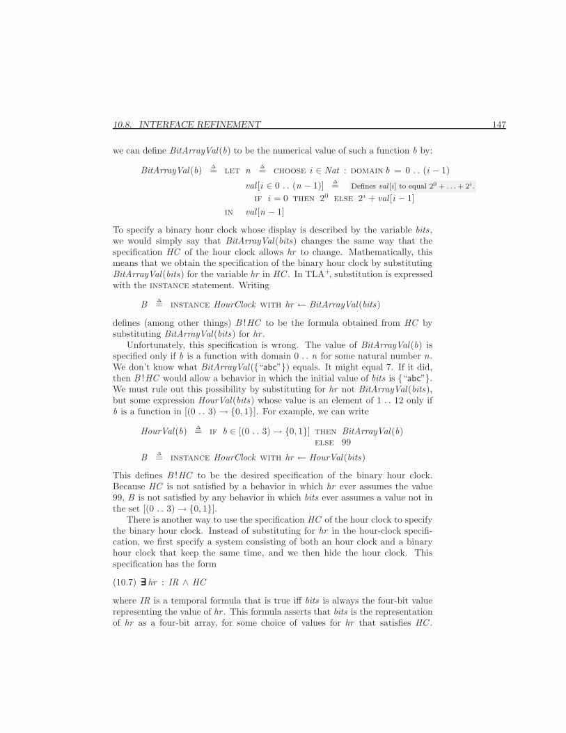
10.8. INTERFACE REFINEMENT 147
we can define BitArrayVal(b) to be the numerical value of such a function b by:
BitArrayVal(b) ∆= let n ∆= choose i ∈ Nat : domain b = 0 . . (i − 1)
val [i ∈ 0 . . (n − 1)] ∆= Defines val [i ] to equal 20 + . . . + 2i .
if i = 0 then 20 else 2i + val [i − 1]in val [n − 1]
To specify a binary hour clock whose display is described by the variable bits ,we would simply say that BitArrayVal(bits) changes the same way that thespecification HC of the hour clock allows hr to change. Mathematically, thismeans that we obtain the specification of the binary hour clock by substitutingBitArrayVal(bits) for the variable hr in HC . In TLA+, substitution is expressedwith the instance statement. Writing
B ∆= instance HourClock with hr ← BitArrayVal(bits)
defines (among other things) B !HC to be the formula obtained from HC bysubstituting BitArrayVal(bits) for hr .
Unfortunately, this specification is wrong. The value of BitArrayVal(b) isspecified only if b is a function with domain 0 . . n for some natural number n.We don’t know what BitArrayVal({“abc”}) equals. It might equal 7. If it did,then B !HC would allow a behavior in which the initial value of bits is {“abc”}.We must rule out this possibility by substituting for hr not BitArrayVal(bits),but some expression HourVal(bits) whose value is an element of 1 . . 12 only ifb is a function in [(0 . . 3)→ {0, 1}]. For example, we can write
HourVal(b) ∆= if b ∈ [(0 . . 3)→ {0, 1}] then BitArrayVal(b)else 99
B ∆= instance HourClock with hr ← HourVal(bits)
This defines B !HC to be the desired specification of the binary hour clock.Because HC is not satisfied by a behavior in which hr ever assumes the value99, B is not satisfied by any behavior in which bits ever assumes a value not inthe set [(0 . . 3)→ {0, 1}].
There is another way to use the specification HC of the hour clock to specifythe binary hour clock. Instead of substituting for hr in the hour-clock specifi-cation, we first specify a system consisting of both an hour clock and a binaryhour clock that keep the same time, and we then hide the hour clock. Thisspecification has the form
∃∃∃∃∃∃ hr : IR ∧ HC(10.7)
where IR is a temporal formula that is true iff bits is always the four-bit valuerepresenting the value of hr . This formula asserts that bits is the representationof hr as a four-bit array, for some choice of values for hr that satisfies HC .
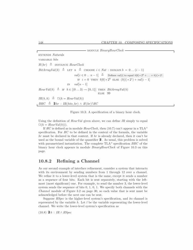
148 CHAPTER 10. COMPOSING SPECIFICATIONS
module BinaryHourClockextends Naturalsvariable bits
H (hr) ∆= instance HourClock
BitArrayVal(b) ∆= let n ∆= choose i ∈ Nat : domain b = 0 . . (i − 1)
val [i ∈ 0 . . n − 1] ∆= Defines val [i ] to equal b[0] ∗ 20 + . . . + b[i ] ∗ 2i .
if i = 0 then b[0] ∗ 20 else (b[i ] ∗ 2i) + val [i − 1]in val [n − 1]
HourVal(b) ∆= if b ∈ [(0 . . 3)→ {0, 1}] then BitArrayVal(b)else 99
IR(b, h) ∆= 2(h = HourVal(b))
BHC ∆= ∃∃∃∃∃∃ hr : IR(bits , hr) ∧ H (hr)!HC
Figure 10.3: A specification of a binary hour clock.
Using the definition of HourVal given above, we can define IR simply to equal2(h = HourVal(b))).
If HC is defined as in module HourClock , then (10.7) can’t appear in a TLA+
specification. For HC to be defined in the context of the formula, the variablehr must be declared in that context. If hr is already declared, then it can’t beused as the bound variable of the quantifier ∃∃∃∃∃∃ . As usual, this problem is solvedwith parametrized instantiation. The complete TLA+ specification BHC of thebinary hour clock appears in module BinaryHourClock of Figure 10.3 on thispage.
10.8.2 Refining a Channel
As our second example of interface refinement, consider a system that interactswith its environment by sending numbers from 1 through 12 over a channel.We refine it to a lower-level system that is the same, except it sends a numberas a sequence of four bits. Each bit is sent separately, starting with the left-most (most significant) one. For example, to send the number 3, the lower-levelsystem sends the sequence of bits 0, 1, 0, 1. We specify both channels with theChannel module of Figure 3.2 on page 30, so each value that is sent must beacknowledged before the next one can be sent.
Suppose HSpec is the higher-level system’s specification, and its channel isrepresented by the variable h. Let l be the variable representing the lower-levelchannel. We write the lower-level system’s specification as
∃∃∃∃∃∃ h : IR ∧ HSpec(10.8)
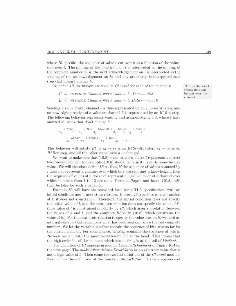
10.8. INTERFACE REFINEMENT 149
where IR specifies the sequence of values sent over h as a function of the valuessent over l . The sending of the fourth bit on l is interpreted as the sending ofthe complete number on h; the next acknowledgement on l is interpreted as thesending of the acknowledgement on h; and any other step is interpreted as astep that doesn’t change h.
To define IR, we instantiate module Channel for each of the channels: Data is the set ofvalues that canbe sent over thechannel.
H ∆= instance Channel with chan ← h, Data ← Nat
L ∆= instance Channel with chan ← l , Data ← −1 . . 9
Sending a value d over channel l is thus represented by an L !Send(d) step, andacknowledging receipt of a value on channel h is represented by an H !Rcv step.The following behavior represents sending and acknowledging a 3, where I haveomitted all steps that don’t change l :
s0
L !Send(0)−→ s1
L !Rcv−→ s2
L !Send(1)−→ s3
L !Rcv−→ s4
L !Send(0)−→
s5
L !Rcv−→ s6
L !Send(1)−→ s7
L !Rcv−→ s8 −→ · · ·This behavior will satisfy IR iff s6 → s7 is an H !Send(3) step, s7 → s8 is anH !Rcv step, and all the other steps leave h unchanged.
We want to make sure that (10.8) is not satisfied unless l represents a correctlower-level channel—for example, (10.8) should be false if l is set to some bizarrevalue. We will therefore define IR so that, if the sequence of values assumed byl does not represent a channel over which bits are sent and acknowledged, thenthe sequence of values of h does not represent a legal behavior of a channel overwhich numbers from 1 to 12 are sent. Formula HSpec, and hence (10.8), willthen be false for such a behavior.
Formula IR will have the standard form for a TLA specification, with aninitial condition and a next-state relation. However, it specifies h as a functionof l ; it does not constrain l . Therefore, the initial condition does not specifythe initial value of l , and the next-state relation does not specify the value of l ′.(The value of l is constrained implicitly by IR, which asserts a relation betweenthe values of h and l , and the conjunct HSpec in (10.8), which constrains thevalue of h.) For the next-state relation to specify the value sent on h, we need aninternal variable that remembers what has been sent on l since the last completenumber. We let the variable bitsSent contain the sequence of bits sent so far forthe current number. For convenience, bitsSent contains the sequence of bits in“reverse order”, with the most recently-sent bit at the head. This means thatthe high-order bit of the number, which is sent first, is at the tail of bitsSent .
The definition of IR appears in module ChannelRefinement of Figure 10.4 onthe next page. The module first defines ErrorVal to be an arbitrary value that isnot a legal value of h. Then come the two instantiations of the Channel module.Next comes the definition of the function BitSeqToNat . If s is a sequence of
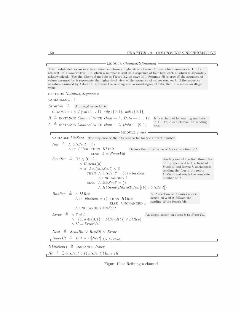
150 CHAPTER 10. COMPOSING SPECIFICATIONS
module ChannelRefinementThis module defines an interface refinement from a higher-level channel h, over which numbers in 1 . . 12are sent, to a lowerer-level l in which a number is sent as a sequence of four bits, each of which is separatelyacknowledged. (See the Channel module in Figure 3.2 on page 30.) Formula IR is true iff the sequence ofvalues assumed by h represents the higher-level view of the sequence of values sent on l . If the sequenceof values assumed by l doesn’t represent the sending and acknowledging of bits, then h assumes an illegalvalue.
extends Naturals ,Sequencesvariables h, l
ErrorVal ∆= An illegal value for h.
choose v : v /∈ [val : 1 . . 12, rdy : {0, 1}, ack : {0, 1}]H ∆= instance Channel with chan ← h, Data ← 1 . . 12
L ∆= instance Channel with chan ← l , Data ← {0, 1}H is a channel for sending numbersin 1 . . 12; L is a channel for sendingbits.
module Innervariable bitsSent The sequence of the bits sent so far for the current number.
Init ∆= ∧ bitsSent = 〈 〉∧ if L !Init then H !Init
else h = ErrorValDefines the initial value of h as a function of l .
SendBit ∆= ∃ b ∈ {0, 1} :∧ L !Send(b)∧ if Len(bitsSent) < 3
then ∧ bitsSent ′ = 〈b 〉 ◦ bitsSent∧ unchanged h
else ∧ bitsSent ′ = 〈 〉∧ H !Send(BitSeqToNat [〈b 〉 ◦ bitsSent ])
Sending one of the first three bitson l prepends it to the front ofbitsSent and leaves h unchanged;sending the fourth bit resetsbitsSent and sends the completenumber on h.
BitsRcv ∆= ∧ L !Rcv∧ if bitsSent = 〈 〉 then H !Rcv
else unchanged h∧ unchanged bitsSent
A Rcv action on l causes a Rcvaction on h iff it follows thesending of the fourth bit.
Error ∆= ∧ l ′ 6= l∧ ¬((∃ b ∈ {0, 1} : L !Send(b)) ∨ L !Rcv)∧ h′ = ErrorVal
An illegal action on l sets h to ErrorVal .
Next ∆= SendBit ∨ RcvBit ∨ Error
InnerIR ∆= Init ∧ 2[Next ]〈 l,h, bitsSent 〉
I (bitsSent) ∆= instance Inner
IR ∆= ∃∃∃∃∃∃ bitsSent : I (bitsSent)!InnerIR
Figure 10.4: Refining a channel.
10.8. INTERFACE REFINEMENT 151
bits, then BitSeqToNat [s ] is its numeric value interpreted as a binary numberwhose low-order bit is at the head of s .
There follows a submodule that defines the internal specification—the one The use of a sub-module to definean internal spec-ification was in-troduced in thereal-time hourclock specificationof Section 9.1.
with the internal variable bitsSent visible. The internal specification’s initialpredicate Init asserts that if l has a legal initial value, then h can have any legalinitial value; otherwise h has an illegal value. Initially bitsSent is the emptysequence 〈 〉. The internal specification’s next-state action is the disjunction ofthree actions:
SendBit A SendBit step is one in which a bit is sent on l . If bitsSent hasfewer than three elements, so fewer than three bits have alreadybeen sent, then the bit is prepended to the head of bitsSent and his left unchanged. Otherwise, the value represented by the four bitssent so far, including the current bit, is sent on h and bitsSent isreset to 〈 〉.
BitsRcv A BitsRcv step is one in which an acknowledgement is sent on l .It represents the sending of an acknowledgement on h iff this is anacknowledgement of the fourth bit, which is true iff bitsSent is theempty sequence.
Error An Error step is one in which an illegal change to l occurs. It setsh to an illegal value.
The inner specification InnerIR has the usual form. (There is no liveness require-ment.) The outer module then instantiates the inner submodule with bitsSentas a parameter, and it defines IR to equal InnerIR with bitsSent hidden.
Now suppose we have a module HigherSpec that defines a specification HSpecof a system that communicates by sending numbers from 1 through 12 over achannel hchan. We obtain, as follows, a lower-level specification LowerSpec inwhich the numbers are sent as sequences of bits on a channel lchan. We firstdeclare lchan and all the variables and constants of the HigherSpec moduleexcept hchan. We then write:
HS (hchan) ∆= instance HigherSpec
IR(h) ∆= instance ChannelRefinement with l ← lchan
LowerSpec ∆= ∃∃∃∃∃∃ h : IR(h)!Spec ∧ HS (h)!IR
10.8.3 Interface Refinement in General
In the examples of the binary clock and of channel refinement, we defined alower-level specification LSpec in terms of a higher-evel one HSpec as:
LSpec ∆= ∃∃∃∃∃∃ h : IR ∧ HSpec(10.9)
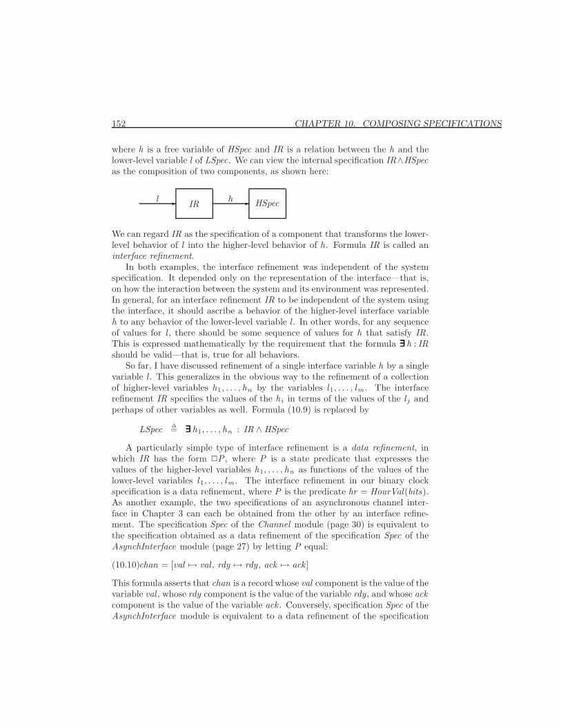
152 CHAPTER 10. COMPOSING SPECIFICATIONS
where h is a free variable of HSpec and IR is a relation between the h and thelower-level variable l of LSpec. We can view the internal specification IR∧HSpecas the composition of two components, as shown here:
l - IR HSpech -
We can regard IR as the specification of a component that transforms the lower-level behavior of l into the higher-level behavior of h. Formula IR is called aninterface refinement.
In both examples, the interface refinement was independent of the systemspecification. It depended only on the representation of the interface—that is,on how the interaction between the system and its environment was represented.In general, for an interface refinement IR to be independent of the system usingthe interface, it should ascribe a behavior of the higher-level interface variableh to any behavior of the lower-level variable l . In other words, for any sequenceof values for l , there should be some sequence of values for h that satisfy IR.This is expressed mathematically by the requirement that the formula ∃∃∃∃∃∃ h : IRshould be valid—that is, true for all behaviors.
So far, I have discussed refinement of a single interface variable h by a singlevariable l . This generalizes in the obvious way to the refinement of a collectionof higher-level variables h1, . . . , hn by the variables l1, . . . , lm . The interfacerefinement IR specifies the values of the hi in terms of the values of the l j andperhaps of other variables as well. Formula (10.9) is replaced by
LSpec ∆= ∃∃∃∃∃∃ h1, . . . , hn : IR ∧ HSpec
A particularly simple type of interface refinement is a data refinement, inwhich IR has the form 2P , where P is a state predicate that expresses thevalues of the higher-level variables h1, . . . , hn as functions of the values of thelower-level variables l1, . . . , lm . The interface refinement in our binary clockspecification is a data refinement, where P is the predicate hr = HourVal(bits).As another example, the two specifications of an asynchronous channel inter-face in Chapter 3 can each be obtained from the other by an interface refine-ment. The specification Spec of the Channel module (page 30) is equivalent tothe specification obtained as a data refinement of the specification Spec of theAsynchInterface module (page 27) by letting P equal:
chan = [val 7→ val , rdy 7→ rdy, ack 7→ ack ](10.10)
This formula asserts that chan is a record whose val component is the value of thevariable val , whose rdy component is the value of the variable rdy, and whose ackcomponent is the value of the variable ack . Conversely, specification Spec of theAsynchInterface module is equivalent to a data refinement of the specification
10.8. INTERFACE REFINEMENT 153
Spec of the Channel module. In this case, defining the state predicate P is alittle tricky. The obvious choice is to let P be the formula GoodVals defined by:
GoodVals ∆= ∧ val = chan.val∧ rdy = chan.rdy∧ ack = chan.ack
However, this can assert that val , rdy, and ack have good values even if chan hasan illegal value—for example, if it is a record with more than three components.Instead, we let P equal
if chan ∈ [val : Data, rdy : {0, 1}, ack : {0, 1}] then GoodValselse BadVals
where BadVals asserts that val , rdy, and ack have some illegal values—thatis, values that are impossible in a behavior satisfying formula Spec of moduleAsynchInterface. (We don’t need such a trick when defining chan as a functionof val , rdy, and ack because our definition (10.10) assures that the value of chanis legal iff the values of all three variables val , rdy, and ack are legal.)
Data refinement is the simplest form of interface refinement. In a morecomplicated interface refinement, the value of the higher-level variables cannotbe expressed as a function of the current values of the lower-level variables. Inthe channel refinement example of Section 10.8.2, the number being sent on thehigher-level channel depends on the values of bits that were previously sent onthe lower-level channel, not just on the lower-level channel’s current state.
We often refine both a system and its interface at the same time. For ex-ample, we may implement a specification H of a system that communicates bysending numbers over a channel with a lower-level specification LImpl of a sys-tem that sends individual bits. In this case, LImpl is not itself obtained fromHSpec by an interface refinement. Rather, LImpl implements some specificationLSpec that is obtained from HSpec by an interface refinement IR. In that case,we say that LImpl implements HSpec under the interface refinement IR.
10.8.4 Open-System Specifications
So far, I have been discussing interface refinement for complete-system specifi-cations. Let’s now consider what happens if the higher-level specification HSpecis the kind of open-system specification discussed in Section 10.7 above. Forsimplicity, we consider the refinement of a single higher-level interface variableh by a single lower-level variable l . The generalization to more variables will beobvious.
Let’s suppose first that HSpec is a safety property, with no liveness condition.As explained in Section 10.7, the specification attributes each change to h eitherto the system or to the environment. Any change to a lower-level interface
154 CHAPTER 10. COMPOSING SPECIFICATIONS
variable l that produces a change to h is therefore attributed to the system orthe environment. A bad change to h that is attributed to the environment makesHSpec true; a bad change that is attributed to the system makes HSpec false.Thus, (10.9) defines LSpec to be an open-system specification. For this to bea sensible specification, the interface refinement IR must ensure that the waychanges to l are attributed to the system or environment is sensible.
If HSpec contains liveness conditions, then interface refinement can be moresubtle. Suppose IR is the interface refinement defined in the ChannelRefinementmodule of Figure 10.4 on page 150, and suppose that HSpec requires that thesystem eventually send some number on h. Consider a behavior in which thesystem sends the first bit of a number on l , but the environment never acknowl-edges it. Under the interface refinement IR, this behavior is interpreted as onein which h never changes. Such a behavior fails to satisfy the liveness conditionof HSpec. Thus, if LSpec is defined by (10.9), then failure of the environment todo something can cause LSpec to be violated, through no fault of the system.
In this example, we want the environment to be at fault if it causes thesystem to halt by failing to acknowledge any of the first three bits of a numbersent by the system. (The acknowledgement of the fourth bit is interpreted by IRas the acknowledgement of a value sent on h, so blame for its absence is properlyassigned to the environment.) Putting the environment at fault means makingLSpec true. We can achieve this by modifying (10.9) to define LSpec as follows:
LSpec ∆= Liveness ⇒ ∃∃∃∃∃∃ h : IR ∧ HSpec(10.11)
where Liveness is a formula requiring that any bit sent on l , other than the lastbit of a number, must eventually be acknowledged. However, if illegal values aresent on l , then we want the safety part of the specification to determine who isresponsible. So, we want Liveness to be true in this case.
Here’s one way to define Liveness . We use the definitions from the Innersubmodule of module ChannelRefinement , where l , h, and bitsSent are visible.The action that acknowledges receipt of one of the first three bits of the numberis BitsRcv∧(bitsSent 6= 〈 〉). Weak fairness of this action asserts that the requiredacknowledgements must eventually be sent. For the case of bad values, recallthat InnerIR implies that sending a bad value on l causes h to equal ErrorVal .We want Liveness to be true if this ever happens, which means if it eventuallyhappens. We therefore add the following definition to the submodule Inner ofthe ChannelRefinement module:
InnerLiveness ∆= ∨ ∧ InnerIR∧ WF〈 l, h, bitsSent 〉(BitsRcv ∧ (bitsSent 6= 〈 〉))
∨ 3(h = ErrorVal)
To define Liveness , we just have to hide h and bitsSent in InnerLiveness . We
10.9. SHOULD YOU COMPOSE? 155
can do this, in a context in which l is declared, as follows:
ICR(h) ∆= instance ChannelRefinementLiveness ∆= ∃∃∃∃∃∃ h, bitsSent : ICR(h)!I (bitsSent)!InnerLiveness
Now, suppose it is the environment that sends numbers over h and the systemis supposed to acknowledge their receipt and then process them in some way. Inthis case, we want failure to acknowledge a bit to be a system error. So, LSpecshould be false if Liveness is. The specification should then be
LSpec ∆= Liveness ∧ (∃∃∃∃∃∃ h : IR ∧ HSpec)
Since h does not occur free in Liveness , this definition is equivalent to
LSpec ∆= ∃∃∃∃∃∃ h : Liveness ∧ IR ∧ HSpec
which has the form (10.9) if the interface refinement IR of (10.9) is taken to beLiveness ∧ IR. In other words, in this case, we make the liveness condition partof the interface refinement.
In general, if HSpec is an open-system specification that describes liveness aswell as safety, then an interface refinement may have to take the form (10.11).Both Liveness and the liveness condition of IR may depend on which changesto the lower-level interface variable l are attributed to the system and which tothe environment. For the channel refinement, this means that they will dependon whether the system or the environment is sending values on the channel.
10.9 Should You Compose?
When specifying a system, should we write a monolithic specification with asingle next-state action, a closed-system composition that is the conjunction ofspecifications of individual components, or an open-system specification? Theanswer is that it usually makes little difference. For a real system, the definitionsof the components’ actions will take hundreds or thousands of lines. The differentforms of specification differ only in the few lines where we assemble the initialpredicates and next-state actions into the final formula.
If you are writing a specification from scratch, it’s probably better to writea monolithic specification. It is usually easier to understand. Of course, thereare exceptions. We write a real-time specification as the conjunction of an un-timed specification and timing constraints; describing the changes to the systemvariables and the timers with a single next-state action usually makes the spec-ification harder to understand.
Writing a composite specification may be sensible when you are starting froman existing specification. If you already have a specification of one component,you may want to write a separate specification of the other component and
156 CHAPTER 10. COMPOSING SPECIFICATIONS
compose the two specifications. If you have a higher-level specification, you maywant to write a lower-level version as an interface refinement. However, theseare rather rare situations. Moreover, it’s likely to be just as easy to modifythe original specification or re-use it in another way. For example, instead ofconjoining a new component to the specification of an existing one, you cansimply include the definition of the existing component’s next-state action, withan extends or instance statement, as part of the new specification.
Composition provides a new way of writing a complete-system specification;it doesn’t change the specification. The choice between a composite specificationand a monolithic one is therefore ultimately a matter of taste. Disjoint-statecompositions are generally straightforward and present no problems. Shared-state compositions can be tricky and require care.
Open-system specifications introduce a mathematically different form of spec-ification. A closed-system specification E ∧M and its open-system counterpartE +−. M are not equivalent. If we really want a specification to serve as a legalcontract between a user and an implementor, then we have to write an open-system specification. We also need open-system specifications if we want tospecify and reason about systems built by composing off-the-shelf componentswith pre-existing specifications. All we can assume about such a component isthat it satisfies a contract between the system builder and the supplier, and sucha contract can be formalized only as an open-system specification. However, youare unlikely to encounter off-the-shelf component specifications during the earlypart of the twenty-first century. In the near future, open-system specificationsare likely to be of theoretical interest only.
Chapter 11
Advanced Examples
It would be nice to provide an assortment of typical examples that cover mostof the specification problems that arise in practice. However, there is no suchthing as a typical specification. Every real specification seems to pose its ownproblems. But we can partition all specifications into two classes, depending onwhether or not they contain variable declarations.
A specification with no variables specifies data structures and operations onthose structures. For example, the Sequences module specifies sequences andvarious operations on them. When specifying a system, you may need somekind of data structure other than the ones provided by the standard moduleslike Sequences and Bags , which are described in Chapter 17. Section 11.1 givesexamples of specifying such data structures.
A system specification contains variables that represent the system’s state.We can further divide system specifications into two classes—high-level specifi-cations that describe what it means for a system to be correct, and lower-levelspecifications that describes what the system actually does. In the memory ex-ample of Chapter 5, the linearizable memory specification of Section 5.3 is ahigh-level specification of correctness, while the write-through cache specifica-tion of Section 5.6 describes how a particular algorithm works. This distinctionis not precise; whether a specification is high- or low-level is a matter of per-spective. But it can be a useful way of categorizing system specifications.
Lower-level system specifications tend to be relatively straightforward. Oncethe level of abstraction has been chosen, writing the specification is usually just amatter of getting the details right when describing what the system does. Spec-ifying high-level correctness can be much more subtle. Section 11.2 considers ahigh level specification problem—formally specifying a multiprocessor memory.
157
158 CHAPTER 11. ADVANCED EXAMPLES
11.1 Specifying Data Structures
Most of the data structures required for writing specifications are mathemati-cally very simple and are easy to define in terms of sets, functions, and records.Section 11.1.2 describes the specification of one such structure—a graph. Onrare occasions, a specification might require sophisticated mathematical con-cepts. The only ones I know of are hybrid system specifications, discussed inSection 9.5. There, we used a module for describing the solutions to differentialequations. That module is specified in Section 11.1.3 below. But, before we getto the specifications of the data structures, we need to learn how to make localdefinitions.
11.1.1 Local Definitions
In the course of specifying a system, we write lots of auxiliary definitions. Asystem specification may consist of a single formula Spec, but we define dozensof other identifiers in terms of which we define Spec. These other identifiers oftenhave fairly common names, and an identifier like Next may be defined in manyspecifications. The different definitions of Next don’t conflict with one anotherbecause, if a system specification is used as part of another specification, theidentifiers it defines are usually renamed. For example, the Channel module isused in module InnerFIFO on page 38 with the statement:
InChan ∆= instance Channel with . . .
The action Next of the Channel module is then instantiated as InChan !Next ,and its definition doesn’t conflict with the definition of Next in the InnerFIFOmodule.
A module that defines operations on a data structure is likely to be incor-porated in another module with an extends statement, without any renam-ing. The module might define some auxiliary operators that are used onlyto define the operators in which we’re interested. For example, we need theDifferentialEquations module only to define the single operator Integrate; butit builds up the definition of Integrate in terms of other operators with nameslike Nbhd and IsDeriv . We don’t want these definitions to conflict with otheruses of those identifiers in a module that extends DifferentialEquations . So, wewant the definitions of Nbhd and IsDeriv to be local to the DifferentialEquationsmodule.
TLA+ provides a local modifier for making definitions local to a module.If a module M contains the definition
local Foo(x ) ∆= . . .
then Foo can be used inside module M just like any ordinary defined identifier.However, a module that extends or instantiates M does not obtain the definition
11.1. SPECIFYING DATA STRUCTURES 159
of Foo. That is, the statement extends M in another module does not defineFoo in that module. Similarly, the statement
N ∆= instance M
does not define N !Foo. The local modifier can also be applied to an instanti-ation. The statement
local instance Sequences
in module M incorporates into M the definitions from the Sequences module.However, another module that extends or instantiates M does not obtain thosedefinitions. The local modifier can be applied only to definitions and instancestatements. It cannot be applied to a declaration or to an extends statement—that is, you cannot write either of the following:
local constant N These are not legal statements.
local extends Sequences
If a module has no constant or variable declarations, then extending it andinstantiating it are equivalent. Thus, the two statements
extends Sequences instance Sequences
are equivalent.In a module that defines general mathematical operators, I like to make all
definitions local except for the ones that we explicitly expect the module tomake. For example, we expect the Sequences module to define operators onsequences, such as Append . We don’t expect it to define operators on numbers,such as +. The Sequences module uses + and other operators defined in theNaturals module. But instead of extending Naturals , it defines those operatorswith the statement
local instance Naturals
The definitions of the operators from Naturals are therefore local to Sequences .A module that uses the Sequences module is then free to define + to meansomething other than addition of numbers.
11.1.2 Graphs
A graphs is an example of the kind of simple data structure often used in specifi-cations. We now write a Graphs module for use in writing system specifications.
We first decide how to represent a graph in terms of data structures thatare already defined—either built-in TLA+ operators or ones defined in existingmodules. Our decision depends on what kind of graphs we want to represent.
160 CHAPTER 11. ADVANCED EXAMPLES
Are we interested in directed graphs or undirected graphs? Finite or infinitegraphs? Graphs with or without self-loops (edges from a node to itself)? Ifwe are specifying graphs for a particular specification, the specification willtell us how to answer these questions. In the absence of such guidance, let’shandle arbitrary graphs. The best way I know of representing both directedand undirected graphs is to specify arbitrary directed graphs, and to definean undirected graph as a directed graph in which every edge has an opposite-pointing edge. Directed graphs have a pretty obvious representation: a directedgraph consists of a set of nodes and a set of edges, where an edge from node mto node n is represented by the ordered pair 〈m, n 〉.
In addition to deciding how to represent graphs, we must decide how tostructure the Graphs module. The decision depends on how we expect themodule to be used. For a specification that uses a single graph, it is mostconvenient to define operations on that specific graph. So, we want the Graphsmodule to have (constant) parameters Node and Edge that represent the sets ofnodes and edges of a particular graph. A specification could use such a modulewith a statement
instance Graphs with Node ← . . . , Edge ← . . .
where the “. . . ”s are the sets of nodes and edges of the particular graph ap-pearing in the specification. On the other hand, a specification might use manydifferent graphs. For example, it might include a formula that asserts the exis-tence of a subgraph, satisfying certain properties, of some given graph G. Sucha specification needs operators that take any graph as an argument—for exam-ple a Subgraph operator defined so SubGraph(G) is the set of all subgraphs ofa graph G. In this case, the Graphs module would have no parameters; spec-ifications would incorporate it with an extends statement. It is this kind ofmodule that we write.
An operator like SubGraph takes a graph as an argument, so we have todecide how to represent a graph as a single value. A graph G consists of a setN of nodes and a set E of edges. A mathematican would represent G as theordered pair 〈N , E 〉. However, G.node is more perspicuous than G[1], so werepresent G as a record with node field N and edge field E .
Having made these decisions, it’s easy to define any standard operator ongraphs. We just have to decide what we should define. Here are some generallyuseful operators:
IsDirectedGraph(G)True iff G is an arbitrary directed graph—that is, a record with nodecomponent N and edge component E such that E is a subset of N × N .This operator is useful because a specification might want to assert thatsomething is a directed graph. (To understand how to assert that G isa record with node and edge fields, see the definition of IsChannel inSection 10.3 on page 129.)
11.1. SPECIFYING DATA STRUCTURES 161
DirectedSubgraph(G)The set of all subgraphs of a directed graph G. Alternatively, we coulddefine IsDirectedSubgraph(H , G) to be true iff H is a subgraph of G. How-ever, it’s easy to express IsDirectedSubgraph in terms of DirectedSubgraph:
IsDirectedSubgraph(H , G) ≡ H ∈ DirectedSubgraph(G)On the other hand, expressing DirectedSubgraph in terms of IsDirectedSubgraphis awkward:
DirectedSubgraph(G) ≡ choose S : ∀H : (H ∈ S ) ≡ IsDirectedSubgraph(H , G)
Note that, as explained in Section 6.1, we can’t define a set of all directedgraphs.
IsUndirectedGraph(G)UndirectedSubgraph(G)
These are analogous to the operators for undirected graphs. As mentionedabove, an undirected graph is a directed graph G such that for everyedge 〈m, n 〉 in G.edge, the inverse edge 〈n, m 〉 is also in G.edge. Notethat DirectedSubgraph(G) contains directed graphs that are not undirectedgraphs.
Path(G)The set of all paths in G, where a path is any sequence of nodes obtainableby following edges. This definition is useful because many properties ofa graph can be expressed in terms of its set of paths. It is convenient toconsider the one-element sequence 〈n 〉 to be a path, for any node n.
AreConnectedIn(m, n, G)True iff there is a path from node m to node n in G. The utility of thisoperator becomes evident when you try defining various common graphproperties, like connectivity.
There are any number of other graph properties and classes of graphs that wemight define. The Graph module defines two:
IsStronglyConnected(G)True iff G is strongly connected, meaning that there is a path from anynode to any other node. For an undirected graph, strongly connected isequivalent to the ordinary definition of connected.
IsTreeWithRoot(G, r)True iff G is a tree with root r , where we represent a tree as a graphwith an edge from each nonroot node to its parent. Thus, the parent of anonroot node n equals:
choose m ∈ G.node : 〈n, m 〉 ∈ G.edge
The Graphs module appears on the next page. By now, you should be able workout for yourself the meanings of all the definitions.
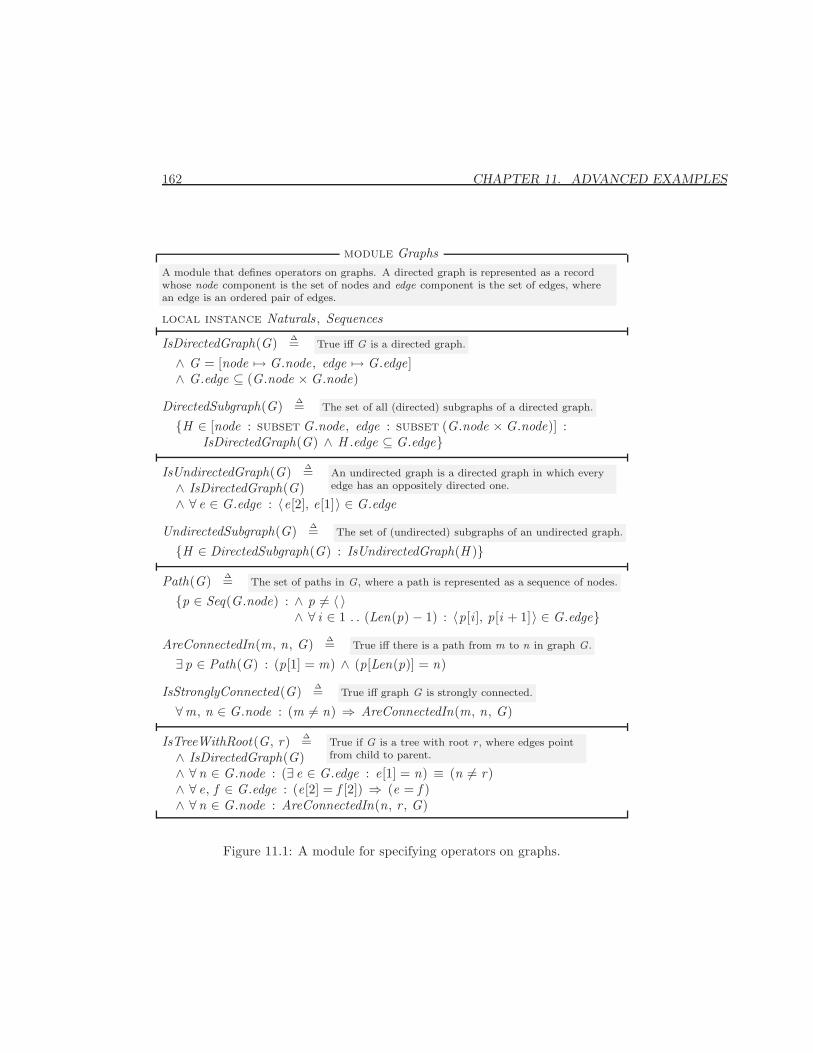
162 CHAPTER 11. ADVANCED EXAMPLES
module GraphsA module that defines operators on graphs. A directed graph is represented as a recordwhose node component is the set of nodes and edge component is the set of edges, wherean edge is an ordered pair of edges.
local instance Naturals , Sequences
IsDirectedGraph(G) ∆= True iff G is a directed graph.
∧ G = [node 7→ G.node, edge 7→ G.edge]∧ G.edge ⊆ (G.node ×G.node)
DirectedSubgraph(G) ∆= The set of all (directed) subgraphs of a directed graph.
{H ∈ [node : subset G.node, edge : subset (G.node ×G.node)] :IsDirectedGraph(G) ∧ H .edge ⊆ G.edge}
IsUndirectedGraph(G) ∆= An undirected graph is a directed graph in which everyedge has an oppositely directed one.∧ IsDirectedGraph(G)
∧ ∀ e ∈ G.edge : 〈e[2], e[1]〉 ∈ G.edge
UndirectedSubgraph(G) ∆= The set of (undirected) subgraphs of an undirected graph.
{H ∈ DirectedSubgraph(G) : IsUndirectedGraph(H )}
Path(G) ∆= The set of paths in G, where a path is represented as a sequence of nodes.
{p ∈ Seq(G.node) : ∧ p 6= 〈 〉∧ ∀ i ∈ 1 . . (Len(p) − 1) : 〈p[i ], p[i + 1]〉 ∈ G.edge}
AreConnectedIn(m, n, G) ∆= True iff there is a path from m to n in graph G.
∃ p ∈ Path(G) : (p[1] = m) ∧ (p[Len(p)] = n)
IsStronglyConnected(G) ∆= True iff graph G is strongly connected.
∀m, n ∈ G.node : (m 6= n) ⇒ AreConnectedIn(m, n, G)
IsTreeWithRoot(G, r) ∆= True if G is a tree with root r , where edges pointfrom child to parent.∧ IsDirectedGraph(G)
∧ ∀n ∈ G.node : (∃ e ∈ G.edge : e[1] = n) ≡ (n 6= r)∧ ∀ e, f ∈ G.edge : (e[2] = f [2]) ⇒ (e = f )∧ ∀n ∈ G.node : AreConnectedIn(n, r , G)
Figure 11.1: A module for specifying operators on graphs.
11.1. SPECIFYING DATA STRUCTURES 163
11.1.3 Solving Differential Equations
Section 9.5 on page 119 describes how to specify a hybrid system whose state in-cludes a physical variable satisfying an ordinary differential equation. The speci-fication uses an operator Integrate such that Integrate(D , t0, t1, 〈x 0, . . . , xn−1 〉)is the value at time t1 of the n-tuple
〈x , dx/dt , . . . , dn−1/dtn−1 〉where x is a solution to the differential equation
D [t , x , dx/dt , . . . , dnx/dtn ] = 0
whose 0th through (n − 1)st derivatives at time t0 are x 0, . . . , xn−1. I nowexplain how to define Integrate. It is an example of the kind of sophisticatedmathematical operators that can be defined in TLA+.
Let’s start by defining some mathematical notation that we will need fordefining the derivative. As usual, we obtain from the Reals module the defini-tions of the set Real of real numbers and of the usual arithmetic operators. LetPosReal be the set of all positive reals:
PosReal ∆= {r ∈ Real : r > 0}and let OpenInterval(a, b) be the open interval from a to b—that is, the set ofnumbers greater than a and less than b:
OpenInterval(a, b) ∆= {s ∈ Real : (a < s) ∧ (s < b)}(Mathematicians usually write this set as (a, b).) Let’s also define Nbhd(r , e)to be the open interval of width 2e centered at r , for e > 0:
Nbhd(r , e) ∆= OpenInterval(r − e, r + e)
For the discussion, we need some notation for the derivative of a function. It’srather difficult to make mathematical sense of the usual notation df /dt for thederivative of f . (What exactly is t?) So, let’s use a mathematically simplernotation. For now, let’s use the fairly conventional mathematical notation ofwriting the nth derivative of the function f as f (n). Recall that f (0), the 0th
derivative of f , equals f .We can now start trying to define Integrate. If a and b are numbers, InitVals
is an n-tuple of numbers, and D is a function from (n +2)-tuples of numbers tonumbers, then
Integrate(D , a, b, InitVals) = 〈f (0)[b], . . . , f (n−1)[b]〉where f is the function satisfying the following two conditions:
• D [r , f (0)[r ], f (1)[r ], . . . , f (n)[r ]] = 0, for all r in some open intervalcontaining a and b.
164 CHAPTER 11. ADVANCED EXAMPLES
• 〈f (0)[a], . . . f (n−1)[a]〉 = InitVals
We want to define Integrate(D , a, b, InitVals) in terms of this function f , whichwe can specify using the choose operator. It’s easiest to choose not just f , butits first n derivatives as well. So, we choose a function g such that g[i ] = f (i) fori ∈ 0 . .n. The function g maps numbers in 0 . .n into functions. More precisely,g is an element of
[0 . . n → [OpenInterval(a − e, b + e)→ Real ] ]
for some positive e. It is the function in this set satisfying the following condi-tions:
• g[i ] is the ith derivative of g[0], for all i ∈ 0 . . n.
• g[i ][a] = InitVals [i ], for all i ∈ 0 . . n.
• D [r , g[0][r ], . . . , g[n][r ] ] = 0, for all r in OpenInterval(a − e, b + e).
To express this last condition formally, without the “. . . ”, we reason as follows:
D [r , g[0][r ], . . . , g[n][r ] ]= D [ 〈r , g[0][r ], . . . , g[n][r ]〉 ] See Section 15.1.7 on page 275.
= D [ 〈r 〉 ◦ 〈g[0][r ], . . . , g[n][r ]〉 ] Tuples are sequences
= D [ 〈r 〉 ◦ [i ∈ 1 . . (n + 1) 7→ g[i − 1][r ]] ] A k -tuple is a function with domain 1 . . k .
So, we can write the formula specifying g as:
∃ e ∈ PosReal : ∧ g ∈ [0 . . n → [OpenInterval(a − e, b + e)→ Real ] ]∧ ∀ i ∈ 1 . . n : ∧ g[i ] = (g[0])(i)
∧ g[i − 1][a] = InitVals [i ]∧ ∀ r ∈ OpenInterval(a − e, b + e) :
D [ 〈r 〉 ◦ [i ∈ 1 . . (n + 1) 7→ g[i − 1][r ]] ] = 0
where n is the length of InitVals . The value of Integrate(D , a, b, InitVals) isthe tuple 〈g[0][b], . . . , g[n − 1][b]〉, which can be written formally as
[i ∈ 1 . . n 7→ g[i − 1][b]]
To complete the definition of Integrate, we have to define the ith derivativeof a function. The derivative is used only in the subformula g[i ] = (g[0])(i).We therefore don’t have to define the ith derivative; we just have to define anoperator that asserts that one function is the ith derivative of another. We definethe operator IsDeriv so that IsDeriv(i , df , f ) is true iff df is the ith derivativeof f . More precisely, IsDeriv(i , df , f ) asserts this if f is i times differentiableon an open interval. We don’t care what IsDeriv(i , df , f ) means if f is not itimes differentiable or its domain is not an open interval.
11.2. OTHER MEMORY SPECIFICATIONS 165
It’s easy to define the ith derivative inductively in terms of the first deriva-tive. So, we define IsFirstDeriv(df , f ) to be true iff df is the first derivative off , assuming that f is a differentiable real-valued function whose domain is anopen subset of the real numbers.1 Elementary calculus tells us that df [r ] is thederivative of f at r iff
df [r ] = lims→r
f [s]− f [r]s− r
The classical “δ-ε” definition of the limit states that this is true iff, for everyε > 0, there is a δ > 0 such that |s − r | < δ implies:∣∣∣∣df [r]− f [s]− f [r]
s− r
∣∣∣∣ < ε
Stated formally, this condition is:
∀ ε ∈ PosReal :∃ δ ∈ PosReal :∀ s ∈ Nbhd(r , δ) \ {r} :
(df [r]− f [s]− f [r]
s− r
)∈ Nbhd(df [r], ε)
We define IsFirstDeriv(df , f ) to be true iff the domains of df and f are equal,and this condition holds for all r in their domain.
The definitions of Integrate and all the other operators introduced aboveappear in the DifferentialEquations module of Figure 11.2 on the next page.The local construct described in Section 11.1.1 above is used to make all thesedefinitions local to the module, except for the definition of Integrate.
11.1.4 The Riemann Integral
To demonstrate how easy it is to formalize ordinary math, we give a specificationof the Riemann integral—the definite integral of elementary calculus. Thoughsometimes written
∫ba f [x ] dx , it’s pretty hard (though by no means impossible)
to make rigorous sense of the dx , so careful mathematicians usually write thisintegral as
∫ba f . The specification is in Figure 11.3 on page 167.
11.2 Other Memory Specifications
Section 5.3 specifies a multiprocessor memory. The specification is unrealisticallysimple for three reasons: a processor can have only one outstanding request at atime, the basic correctness condition is too restrictive, and only simple read and
1A subset S of the real numbers is open iff, for every r ∈ S , there exists an ε > 0 such thatthe interval from r − ε to r + ε is contained in S .

166 CHAPTER 11. ADVANCED EXAMPLES
module DifferentialEquations
This module defines the operator Integrate for specifying the solution to a differential equation. If a and b arereals with a ≤ b; InitVals is an n−tuple of reals; and D is a function from (n + 1)−tuples of reals to reals; thenthis is the n−tuple of values
〈f [b],df
dt[b], . . . ,
dn−1f
dtn−1[b]〉
where f is the solution to the differential equation
D [t , f ,df
dt, . . . ,
dn f
dtn] = 0
such that
〈f [a],df
dt[a], . . . ,
dn−1f
dtn−1[a]〉 = InitVals
local instance Reals , Sequences
local PosReal ∆= {r ∈ Real : r > 0}local OpenInterval(a, b) ∆= {s ∈ Real : (a < s) ∧ (s < b)}local Nbhd(r , e) ∆= OpenInterval(r − e, r + e)
The instance statement andthese definitions are local, so amodule that extends this oneobtains only the definitions ofDeriv and Integrate.
local IsFirstDeriv(df , f ) ∆= Assuming domain f is an open subset of Real , this is true ifff is differentiable and g is its first derivative. Recall that thederivative of f at r is the number df [r ] satisfying the followingcondition: for every ε there exists a δ such that 0 < |s − r | < δimplies |df [r ] − (f [s] − f [r ])/(s − r)| < ε.
∧ df ∈ [domain f → Real ]∧ ∀ r ∈ domain f :
∀ e ∈ PosReal :∃ d ∈ PosReal :∀ s ∈ Nbhd(r , d) \ {r} : (f [s ]− f [r ])/(s − r) ∈ Nbhd(df [r ], e)
local IsDeriv(n, df , f ) ∆= True iff f is n times differentiable and df is its nth derivative.
let IsD [k ∈ 0 . . n, dg, g ∈ [domain f → Real ] ] ∆=if k = 0 then dg = g
else ∃ gg ∈ [domain f → Real ] : ∧ IsFirstDeriv(dg, g)∧ IsD [k − 1, dg, gg]
in IsD [n, df , f ]
Integrate(D , a, b, InitVals) ∆=let n ∆= Len(InitVals)
gg ∆= choose g :∃ e ∈ PosReal : ∧ g ∈ [0 . . n → [OpenInterval(a − e, b + e)→ Real ] ]
∧ ∀ i ∈ 1 . . n : ∧ IsDeriv(i , g[i ], g[0])∧ g[i − 1][a] = InitVals [i ]
∧ ∀ r ∈ OpenInterval(a − e, b + e) :D [ 〈r 〉 ◦ [i ∈ 1 . . (n + 1) 7→ g[i − 1][r ]] ] = 0
in [i ∈ 1 . . n 7→ gg[i − 1][b]]
Figure 11.2: A module for specifying the solution to a differential equation.
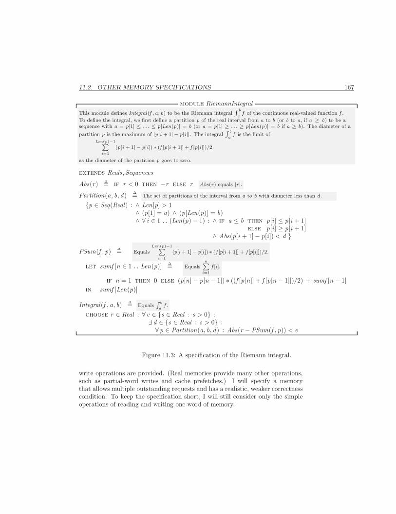
11.2. OTHER MEMORY SPECIFICATIONS 167
module RiemannIntegralThis module defines Integral(f , a, b) to be the Riemann integral
∫ b
af of the continuous real-valued function f .
To define the integral, we first define a partition p of the real interval from a to b (or b to a, if a ≥ b) to be asequence with a = p[1] ≤ . . . ≤ p[Len(p)] = b (or a = p[1] ≥ . . . ≥ p[Len(p)] = b if a ≥ b). The diameter of a
partition p is the maximum of |p[i + 1] − p[i ]|. The integral∫ b
af is the limit of
Len(p)−1∑i=1
(p[i + 1] − p[i ]) ∗ (f [p[i + 1]] + f [p[i ]])/2
as the diameter of the partition p goes to zero.
extends Reals ,Sequences
Abs(r) ∆= if r < 0 then −r else r Abs(r) equals |r |.
Partition(a, b, d) ∆= The set of partitions of the interval from a to b with diameter less than d .
{p ∈ Seq(Real) : ∧ Len[p] > 1∧ (p[1] = a) ∧ (p[Len(p)] = b)∧ ∀ i ∈ 1 . . (Len(p) − 1) : ∧ if a ≤ b then p[i ] ≤ p[i + 1]
else p[i ] ≥ p[i + 1]∧ Abs(p[i + 1]− p[i ]) < d }
PSum(f , p) ∆= EqualsLen(p)−1∑
i=1
(p[i + 1] − p[i]) ∗ (f [p[i + 1]] + f [p[i]])/2.
let sumf [n ∈ 1 . . Len(p)] ∆= Equalsn∑
i=1
f [i].
if n = 1 then 0 else (p[n] − p[n − 1]) ∗ ((f [p[n]] + f [p[n − 1]])/2) + sumf [n − 1]in sumf [Len(p)]
Integral(f , a, b) ∆= Equals∫ b
af .
choose r ∈ Real : ∀ e ∈ {s ∈ Real : s > 0} :∃ d ∈ {s ∈ Real : s > 0} :∀ p ∈ Partition(a, b, d) : Abs(r − PSum(f , p)) < e
Figure 11.3: A specification of the Riemann integral.
write operations are provided. (Real memories provide many other operations,such as partial-word writes and cache prefetches.) I will specify a memorythat allows multiple outstanding requests and has a realistic, weaker correctnesscondition. To keep the specification short, I will still consider only the simpleoperations of reading and writing one word of memory.
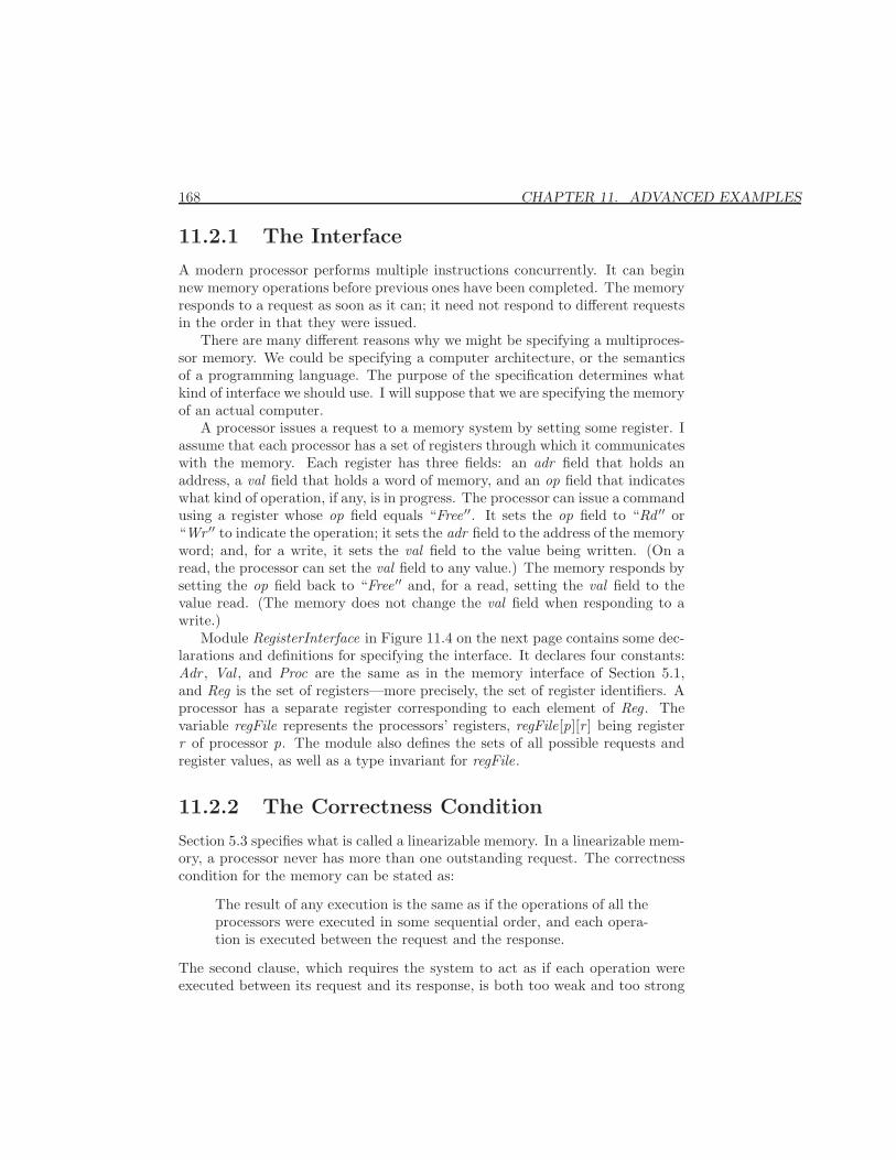
168 CHAPTER 11. ADVANCED EXAMPLES
11.2.1 The Interface
A modern processor performs multiple instructions concurrently. It can beginnew memory operations before previous ones have been completed. The memoryresponds to a request as soon as it can; it need not respond to different requestsin the order in that they were issued.
There are many different reasons why we might be specifying a multiproces-sor memory. We could be specifying a computer architecture, or the semanticsof a programming language. The purpose of the specification determines whatkind of interface we should use. I will suppose that we are specifying the memoryof an actual computer.
A processor issues a request to a memory system by setting some register. Iassume that each processor has a set of registers through which it communicateswith the memory. Each register has three fields: an adr field that holds anaddress, a val field that holds a word of memory, and an op field that indicateswhat kind of operation, if any, is in progress. The processor can issue a commandusing a register whose op field equals “Free′′. It sets the op field to “Rd ′′ or“Wr ′′ to indicate the operation; it sets the adr field to the address of the memoryword; and, for a write, it sets the val field to the value being written. (On aread, the processor can set the val field to any value.) The memory responds bysetting the op field back to “Free′′ and, for a read, setting the val field to thevalue read. (The memory does not change the val field when responding to awrite.)
Module RegisterInterface in Figure 11.4 on the next page contains some dec-larations and definitions for specifying the interface. It declares four constants:Adr , Val , and Proc are the same as in the memory interface of Section 5.1,and Reg is the set of registers—more precisely, the set of register identifiers. Aprocessor has a separate register corresponding to each element of Reg. Thevariable regFile represents the processors’ registers, regFile[p][r ] being registerr of processor p. The module also defines the sets of all possible requests andregister values, as well as a type invariant for regFile.
11.2.2 The Correctness Condition
Section 5.3 specifies what is called a linearizable memory. In a linearizable mem-ory, a processor never has more than one outstanding request. The correctnesscondition for the memory can be stated as:
The result of any execution is the same as if the operations of all theprocessors were executed in some sequential order, and each opera-tion is executed between the request and the response.
The second clause, which requires the system to act as if each operation wereexecuted between its request and its response, is both too weak and too strong
11.2. OTHER MEMORY SPECIFICATIONS 169
module RegisterInterfaceconstant Adr , The set of memory addresses.
Val , The set of memory-word values.
Proc, The set of processors used by a processor.
Reg The set of registers.
variable regFile regFile[p][r ] represents the contents of register r of processor p.
RdRequest ∆= [adr : Adr , val : Val , op : {“Rd”}]WrRequest ∆= [adr : Adr , val : Val , op : {“Wr”}]FreeRegValue ∆= [adr : Adr , val : Val , op : {“Free”}]Request ∆= RdRequest ∪WrRequest The set of all possible requests.
RegValue ∆= Request ∪ FreeRegValue The set of all possible register values.
RegFileTypeInvariant ∆= The type correctness invariant for regFile.
regFile ∈ [Proc → [Reg → RegValue]]
Figure 11.4: A module for specifying a register interface to a memory.
for our specification. It’s too weak because it says nothing about the executionorder of two operations from the same processor unless one is issued after theother’s response. For example, suppose a processor p issues a write and then aread to the same address. We want the read to obtain either the value p justwrote, or a value written by another processor—even if p issues the read beforereceiving the response for the write. This isn’t guaranteed by the condition.The clause is too strong because it places unnecessary ordering constraints onoperations issued by different processors. If operations A and B are issued bytwo different processors, then we don’t need to require that A precedes B in theexecution order just because B was requested after A’s response.
We modify the second clause to require that the system act as if operationsof each individual processor were executed in the order that they were issued:
The result of any execution is the same as if the operations of allthe processors were executed in some sequential order, and the op-erations of each individual processor appear in this sequence in theorder in which the requests were issued.
In other words, we require that the values returned by the reads can be explainedby some total ordering of the operation executions that is consistent with theorder in which each processor issued its requests. There are a number of differentways of formalizing this definition, which differ in how bizarre the explanationmay be. The differences can be described in terms of whether or not certainscenarios are permitted. So, let’s introduce some notation for writing scenarios.
170 CHAPTER 11. ADVANCED EXAMPLES
Let Wrp(a, v) represent a write operation of value v to address a by processorp, and let Rdp(a, v) represent a read of a by p that returns the value v .
The first decision we must make is whether all operations in an infinitebehavior must be ordered, or if the ordering must exist only at each finite pointduring the behavior. Consider a scenario in which each of two processes writesits own value to the same address and then keeps reading that value forever: In these scenar-
ios, I assume thatvalues and ad-dresses with dif-ferent names aredifferent.
Process p : Wrp(a, v1), Rdp(a, v1), Rdp(a, v1), Rdp(a, v1), . . .
Process q : Wrq(a, v2), Rdq(a, v2), Rdq(a, v2), Rdq(a, v2), . . .
At each point in the execution, we can explain the values returned by the readswith a total order in which all the operations of either processor precede all theoperations of the other. However, there is no way of explaining the entire infinitescenario with a single total order. In this scenario, neither processor ever seesthe value written by the other. Since a multiprocessor memory is supposed toallow processors to communicate, we disallow this scenario.
The second decision we must make is whether the memory is allowed topredict the future. Consider this scenario:
Processor p : Wrp(a, v1), Rdp(a, v2)Processor q : Wrq(a, v2)
Here, q issues its write of v2 after p has obtained the result of its read. Thescenario is explained by the ordering Wrp(a, v1), Wrq(a, v2), Rdp(a, v2). How-ever, this is a bizarre explanation because, to return the value v2 for p’s read,the memory had to predict that another processor would write v2 some time inthe future. Since a real memory can’t predict what requests will be issued inthe future, such a behavior cannot be produced by a correct implementation.We can therefore rule out the scenario as unreasonable. Alternatively, since nocorrect implementation can produce it, there’s no need to outlaw the scenario.
If we don’t allow the memory to predict the future, then it must always beable to explain the values read in terms of the writes that have been issued sofar. In this case, we have to decide whether the explanations must be stable.For example, suppose a scenario begins as follows:
Processor p : Wrp(a1, v1), Rdp(a1, v3)Processor q : Wrq(a2, v2), Wrq(a1, v3)
At this point, the only explanation for p’s read Rdp(a1, v3) is that q’s writeWrq(a1, v3) preceded it, which implies that q’s other write Wrq(a2, v2) alsopreceded the read. Hence, if p now reads a2, it must obtain the value v2. Butsuppose the scenario continues as follows, with another processor r joining in:
Processor p : Wrp(a1, v1), Rdp(a1, v3), Rdp(a2, v0)Processor q : Wrq(a2, v2), Wrq(a1, v3)Processor r : Wrr(a1, v3)
11.2. OTHER MEMORY SPECIFICATIONS 171
We can explain this scenario with the following ordering of the operations:
Wrp(a1, v1), Wr r (a1, v3), Rdp(a1, v3), Rdp(a2, v0), Wrq(a2, v2), Wrq(a1, v3)
In this explanation, processor r provided the value of a1 read by p, and p readthe initial value v0 of memory address a2. The explanation of the value ofa1 read by p thus changes in mid-execution. Should we allow explanations tochange in this way?
11.2.3 A Serial Memory
We first specify a memory that cannot predict the future and cannot change itsexplanations. There seems to be no standard name for such a memory; I’ll callit serial.
The informal correctness condition is in terms of the sequence of all opera-tions that have ever been issued. There is a general method of formalizing sucha condition that works for specifying many different kinds of systems. We addan internal variable opQ that records the history of the execution. For eachprocessor p the value of opQ [p] is a sequence, where opQ [p][i ] describes the ith
request issued by p, the response to the request (if it has been issued), and anyother information about the operation needed to express the correctness con-dition. We can also add one or more additional internal variables that recordadditional information not readily associated with the individual operations.
For a system with the kind of register interface we are using, the next-staterelation has the form
∨ ∃ proc ∈ Proc, reg ∈ Reg : ∨ ∃ req ∈ Request : IssueRequest(proc, req, reg)∨ RespondToRequest(proc, reg)
∨ Internal
(11.1)
where the component actions do the following:
IssueRequest(proc, req, reg)The action with which processor proc issues a request req in register reg.
RespondToRequest(proc, reg)The action with which the system responds to a request in processor proc’sregister reg.
InternalAn action that changes only the internal state.
Liveness properties are asserted by fairness conditions on the RespondToRequestand Internal actions.
A general trick for writing the specification is to choose the internal state sothe safety part of the correctness condition can be expressed by the formula 2P
172 CHAPTER 11. ADVANCED EXAMPLES
for some state predicate P ; and the liveness part can be expressed by fairnesson the Internal action. We guarantee that P is always true by letting P ′ bea conjunct of each action. I’ll use this approach to specify the serial memory,taking for P a state predicate will be called Serializable.
We want to require that the value returned by each read is explainable asthe value written by some operation already issued, or as the initial value of thememory. Moreover, we don’t want this explanation to change. We therefore addto the opQ entry for each completed read a source field that indicates where thevalue came from. This field is set by the RespondToRequest action.
We want all operations in an infinite behavior eventually to be ordered. Thismeans that, for any two operations, the memory must eventually decide whichone precedes the other—and it must stick to that decision. We introduce aninternal variable opOrder that describes the ordering of operations to which thememory has already committed itself. An Internal step changes only opOrder ,and it can only enlarge the ordering.
The predicate Serializable used to specify the safety part of the correctnesscondition describes what it means for opOrder to be a correct explanation. Itasserts that there is some consistent total ordering of the operations that satisfiesthe following conditions:
• It extends opOrder .
• It orders all operations from the same processor in the order that theywere issued.
• It orders operations so that the source of any read is the latest write tothe same address that precedes the read, and is the initial value iff thereis no such write.
We now translate this informal sketch of the specification into TLA+. Wefirst choose the types of the variables opQ and opOrder . To describe the sourcefield of a read and an order on operations, we define a set opId of values thatdescribe the operations that have been issued. An operation is specified by apair 〈p, i 〉 where p is a processor and i is a position in the sequence opQ [p].(The set of all such positions i is domain opQ [p].) We let the correspondingelement of opId be the record with proc field p and idx field i , so we define:
opId ∆= {oiv ∈ OpIdVal : oiv .idx ∈ domain opQ [oiv .proc]}For convenience, we define opIdQ(oi) to be the value of the opQ entry denotedby an element oi of opId :
opIdQ(oi) ∆= opQ [oi .proc][oi .idx ]
The source of a value need not be an operation; it can also be the inital contentsof the memory. The latter possibility is represented by letting the source fieldof the opQ entry have the special value InitWr . We then let opQ be an elementof [Proc → Seq(opVal)], where opVal is the union of three sets: WrRequest ,
RdRequest , andRequest are de-fined in moduleRegisterInterfaceon page 169.
11.2. OTHER MEMORY SPECIFICATIONS 173
[req : Request , reg : Reg]Represents an active request in the register of the requesting processorindicated by the reg field.
[req : WrRequest , reg : {Done}]Represents a completed write request, where Done is a special value thatis not a register.
[req : RdRequest , reg : {Done}, source : opId ∪ {InitWr}]Represents a completed read request whose value came from the operationindicated by the source field, or from the initial value of the memorylocation if the source field equals InitWr .
Observe that opId and opVal are state functions whose values depend upon thevalue of the variable opQ .
We need to specify the initial value of memory. A program generally cannotassume anything about the memory’s initial value, except that every addressdoes contain a value in Val . So, the initial value value of memory can be anyelement of [Adr → Val ]. We declare an “internal” constant InitMem, whosevalue is the initial memory value. In the final specification, InitMem will behidden along with the internal variables opQ and opOrder . We hide a constantwith ordinary existential quantification ∃ . The requirement that InitMem is afunction from addresses to values could be made part of the initial predicate,but it’s more natural to express it in the quantifier. The final specification willtherefore have the form:
∃ InitMem ∈ [Adr → Val ] : ∃∃∃∃∃∃ opQ , opOrder : . . .
For later use, we define goodSource(oi) to be the set of plausible values forthe source of a read operation oi in opId . By a plausible value, I mean eitherInitWr or a write to the same address that oi reads. It will be an invariantof the specification that the source of any completed read operation oi is anelement of goodSource(oi). Moreover, if the source of oi is InitWr , then therequest’s value must equal the value assigned to the address by InitMem. Toexpress this formally, observe that only the opQ entries of completed reads havea source field. Since a record has a source field iff the string “source” is in itsdomain, we can write this invariant as:
Section 5.2 onpage 48 explainsthat a record isa function whosedomain is a set ofstrings.
∀ oi ∈ opId :(“source” ∈ domain opIdQ(oi)) ⇒∧ opIdQ(oi).source ∈ goodSource(oi)∧ (opIdQ(oi).source = InitWr) ⇒ (opIdQ(oi).req.val = InitMem[opIdQ(oi).req.adr ])
(11.2)
We now choose the type of opOrder . We usually represent an ordering relationas an operator such as ≺, writing A ≺ B to mean that A precedes B . However,the value of a variable cannot be an operator. So, we must represent an ordering The difference
between oper-ators and func-tions is discussedin Section 6.4 onpage 69.
174 CHAPTER 11. ADVANCED EXAMPLES
relation as a set or a function. Mathematicians usually describe a relation ≺ ona set S as a set R of ordered pairs of elements in S , with 〈A, B 〉 in R iff A ≺ B .So, we let opOrder be a subset of opId × opId , where 〈oi , oj 〉 ∈ opOrder meansthat oi precedes oj .
Our internal state is redundant because, if register r of processor p containsan uncompleted operation, then there is an opQ entry that points to the regis-ter and contains the same request. This redundancy means that the followingrelations among the variables are invariants of the specification:
• If an opQ entry’s reg field is not equal to Done, then it denotes a registerwhose contents is the entry’s req field.
• The number of opQ entries pointing to a register equals 1 if the registercontains an active operation, otherwise it equals 0.
In the specification, we combine this condition, formula (11.2), and the typeinvariant into a single state predicate DataInvariant .
Having chosen the types of the variables, we can now define the initial predi-cate Init and the predicate Serializable. The definition of Init is easy. We defineSerializable in terms of totalOpOrder , the set of all total orderings of opId . Arelation ≺ is a total ordering of opId iff it satisfies the following three conditions,for any oi , oj , and ok in opId .
Totality: Either oi = oj , oi ≺ oj , or oj ≺ oi .
Transitivity: oi ≺ oj and oj ≺ ok imply oi ≺ ok .
Irreflexivity: oi 6≺ oi .
The predicate Serializable asserts that there is a total ordering of opId satisfyingthe three conditions on page 172. We can express this formally as the assertionthat there exists an R in totalOpOrder satisfying:
∧ opOrder ⊆ R R extends opOrder
∧ ∀ oi , oj ∈ opId : R correctly orders operations from the same processor.
(oi .proc = oj .proc) ∧ (oi .idx < oj .idx ) ⇒ (〈oi , oj 〉 ∈ R)
∧ ∀ oi ∈ opId : For every completed read oi in opId , there is no writeoj to the same address that (i) precedes oi and(ii) follows the source if that source is not InitWr .
(“source” ∈ domain opIdQ(oi))⇒ ¬ (∃ oj ∈ goodSource(oi) :
∧ 〈oj , oi 〉 ∈ R∧ (opIdQ(oi).source 6= InitWr) ⇒ (〈opIdQ(oi).source, oj 〉 ∈ R) )
We allow each step to extend opOrder to any relation on opId that satisfiesSerializable. We do this by letting every subaction of the next-state action
11.2. OTHER MEMORY SPECIFICATIONS 175
specify opOrder ′ with the conjunct UpdateOpOrder , defined by:
UpdateOpOrder ∆= ∧ opOrder ′ ⊆ (opId ′ × opId ′)∧ opOrder ⊆ opOrder ′
∧ Serializable′
The next-state action has the generic form of formula (11.1) on page 171. Wesplit the RespondToRequest action into the disjunction of separate RespondToWrand RespondToRd actions that represent responding to writes and reads, respec-tively. RespondToRd is the most complicated of the next-state action’s subac-tions, so let’s examine its definition. The definition has the form:
RespondToRd(proc, reg) ∆=let req ∆= regFile[proc][reg]
idx ∆= choose i ∈ domain opQ [proc] : opQ [proc][i ].reg = regin . . .
This defines req to be the request in the register and idx to be an element inthe domain of opQ [proc] such that opQ [proc][idx ].reg equals reg. If the registeris not free, then there is exactly one such idx ; and opQ [proc][idx ].req, the idx th
request issued by proc, equals req. (We don’t care what idx equals if the registeris free.) The in expression begins with the enabling condition:
∧ req.op = “Rd”
which asserts that the register is not free and it contains a read request. Thenext conjunct of the in expression is:
∧ ∃ src ∈ goodSource([proc 7→ proc, idx 7→ idx ]) :∧ let val ∆= if src = InitWr then InitMem[req.adr ]
else opIdQ(src).req.valin . . .
It asserts the existence of a value src, which will be the source of the valuereturned by the read; and it defines val to be that value. If the source is theinitial value of memory, then the value is obtained from InitMem; otherwise,it is obtained from the source request’s val field. The inner in expression hastwo conjuncts that specify the values of regFile′ and opQ ′. The first conjunctasserts that the register’s val field is set to val and its op field is set to “Free”,indicating that the register is made free.
∧ regFile′ = [regFile except ! [proc][reg].val = val ,! [proc][reg].op = “Free”]
The second conjunct of the inner in expression describes the new value of opQ .Only the idx th element of opQ [proc] is changed. It is set to a record whose req
176 CHAPTER 11. ADVANCED EXAMPLES
field is the same as the original request req, except that its val field is equal toval ; whose reg field equals Done; and whose source field equals src.
∧ opQ ′ = [opQ except ! [proc][idx ] = [req 7→ [req except !.val = val ],reg 7→ Done,source 7→ src] ]
Finally, the outer in clause ends with the conjunct
∧ UpdateOpOrder
that determines the value of opOrder ′. It also implicitly determines the possiblechoices of the source of the read—that is, the value of opQ ′[proc][idx ].source.For some choices of this value allowed by the second outer conjunct, there will beno value of opOrder ′ satisfying UpdateOpOrder . The conjunct UpdateOpOrderrules out those choices for the source.
The definitions of the other subactions of the next-state action—IssueRequest ,RespondtoWr , and Internal—are simpler and I won’t explain them.
Having finished the initial predicate and the next-state action, we must deter-mine the liveness conditions. The first condition is that the memory must eventu-ally respond to every operation. The response to a request in register reg of pro-cessor proc is produced by a RespondToWr(proc, reg) or RespondToRd(proc, reg)action. So, the obvious way to express this condition is:
∀ proc ∈ Proc, reg ∈ Reg :WF〈 ...〉(RespondToWr(proc, reg) ∨ RespondToRd(proc, reg))
For this to imply that the response is eventually issued, RespondToWr(proc, reg)or RespondToRd(proc, reg) must be enabled if there is an uncompleted operationin proc’s register reg. This isn’t completely obvious for a read request, becauseRespondToRd(proc, reg) is enabled only if there exist a source for the read and avalue of opOrder ′ that satisfy Serializable′. They do exist because Serializable,which holds in the initial state, implies the existence of a correct total orderingof all the operations; this ordering can be used to choose a source and a relationopOrder ′ that satisfy Serializability ′ .
The second liveness condition is that the memory must eventually commit toan ordering for every pair of operations. This is expressed as a fairness condition,for every pair of distinct operations oi and oj in opId , on an Internal action thatmakes oi either precede or follow oj in the ordering opOrder ′. A first attemptat this condition is
∀ oi , oj ∈ opId : (oi 6= oj ) ⇒ WF〈 ...〉(∧ Internal∧ (〈oi , oj 〉 ∈ opOrder ′) ∨ (〈oj , oi 〉 ∈ opOrder ′))
(11.3)
11.2. OTHER MEMORY SPECIFICATIONS 177
However, this isn’t correct. In general, a formula ∀ x ∈ S : F is equivalent to∀ x : (x ∈ S )⇒ F . Hence, (11.3) is equivalent to the assertion that the followingformula holds, for all constant values oi and oj :
(oi ∈ opId) ∧ (oj ∈ opId) ⇒(oi 6= oj ) ⇒ WF〈 ...〉(∧ Internal
∧ (〈oi , oj 〉 ∈ opOrder ′) ∨ (〈oj , oi 〉 ∈ opOrder ′))
In a temporal formula, a predicate with no temporal operators is an assertionabout the initial state. Hence, (11.3) asserts that the fairness condition is truefor all pairs of distinct values oi and oj in the initial value of opId . But opIdis initially empty, so this condition is vacuously true. Hence, (11.3) is triviallyimplied by the initial predicate. We must instead assert fairness for the action
∧ (oi ∈ opId) ∧ (oj ∈ opId)∧ Internal∧ (〈oi , oj 〉 ∈ opOrder ′) ∨ (〈oj , oi 〉 ∈ opOrder ′))
(11.4)
for all distinct values oi and oj . It suffices to assert this only for oi and oj ofthe right type. Since I prefer using bounded quantifiers whenever possible, I willwrite this condition as:
∀ oi , oj ∈ [proc : Proc, idx : Nat ] : All operations are eventually ordered.
(oi 6= oj ) ⇒ WF〈 ...〉(∧ (oi ∈ opId) ∧ (oj ∈ opId)∧ Internal∧ (〈oi , oj 〉 ∈ opOrder ′) ∨ (〈oj , oi 〉 ∈ opOrder ′))
For this formula to imply that any two operations are eventually ordered byopOrder , action (11.4) must be enabled if oi and oj are unordered operationsin opId . It is, because Serializable is always enabled, so it is always possible toextend opOrder to a total ordering of all issued operations.
The complete inner specification, with InitMem, opQ , and opOrder visible, isin module InnerSerial on pages 179–181. I have made two minor modificationsto allow the specification to be checked by the TLC model checker. (Chap-ter 13 describes TLC and explains why these changes are needed.) Instead ofthe definition of opId given on page 172, the specification uses the equivalentdefinition:
opId ∆= union { [proc : p, idx : domain opQ [p] ]}In the definition of UpdateOpOrder , the first conjunct is changed from
opOrder ′ ⊆ opId ′ × opId ′
to the equivalent
opOrder ′ ∈ subset (opId ′ × opId ′)
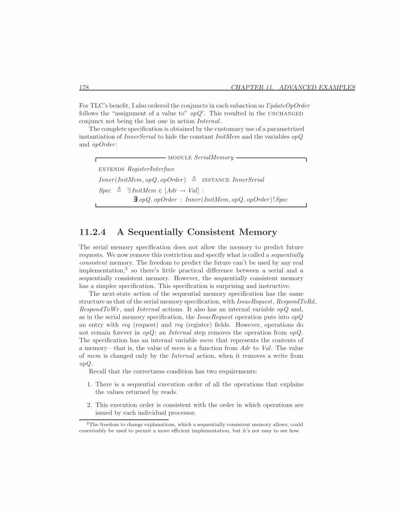
178 CHAPTER 11. ADVANCED EXAMPLES
For TLC’s benefit, I also ordered the conjuncts in each subaction so UpdateOpOrderfollows the “assignment of a value to” opQ ′. This resulted in the unchangedconjunct not being the last one in action Internal .
The complete specification is obtained by the customary use of a parametrizedinstantiation of InnerSerial to hide the constant InitMem and the variables opQand opOrder :
module SerialMemory
extends RegisterInterface
Inner(InitMem, opQ , opOrder) ∆= instance InnerSerial
Spec ∆= ∃ InitMem ∈ [Adr → Val ] :∃∃∃∃∃∃ opQ , opOrder : Inner(InitMem, opQ , opOrder)!Spec
11.2.4 A Sequentially Consistent Memory
The serial memory specification does not allow the memory to predict futurerequests. We now remove this restriction and specify what is called a sequentiallyconsistent memory. The freedom to predict the future can’t be used by any realimplementation,2 so there’s little practical difference between a serial and asequentially consistent memory. However, the sequentially consistent memoryhas a simpler specification. This specification is surprising and instructive.
The next-state action of the sequential memory specification has the samestructure as that of the serial memory specification, with IssueRequest , RespondToRd ,RespondToWr , and Internal actions. It also has an internal variable opQ and,as in the serial memory specification, the IssueRequest operation puts into opQan entry with req (request) and req (register) fields. However, operations donot remain forever in opQ ; an Internal step removes the operation from opQ .The specification has an internal variable mem that represents the contents ofa memory—that is, the value of mem is a function from Adr to Val . The valueof mem is changed only by the Internal action, when it removes a write fromopQ .
Recall that the correctness condition has two requirements:
1. There is a sequential execution order of all the operations that explainsthe values returned by reads.
2. This execution order is consistent with the order in which operations areissued by each individual processor.
2The freedom to change explanations, which a sequentially consistent memory allows, couldconceivably be used to permit a more efficient implementation, but it’s not easy to see how.
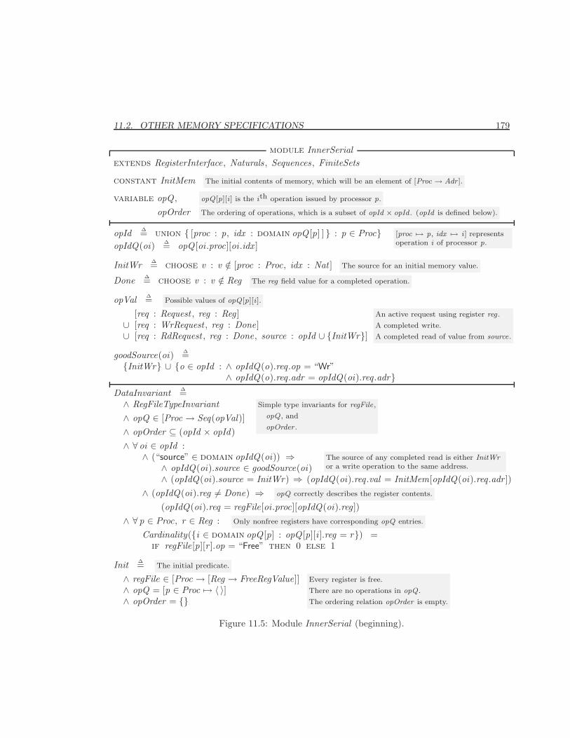
11.2. OTHER MEMORY SPECIFICATIONS 179
module InnerSerialextends RegisterInterface, Naturals , Sequences , FiniteSets
constant InitMem The initial contents of memory, which will be an element of [Proc → Adr ].
variable opQ , opQ [p][i ] is the ith operation issued by processor p.
opOrder The ordering of operations, which is a subset of opId × opId . (opId is defined below).
opId ∆= union { [proc : p, idx : domain opQ [p] ] } : p ∈ Proc}opIdQ(oi) ∆= opQ [oi .proc][oi .idx ]
[proc 7→ p, idx 7→ i ] representsoperation i of processor p.
InitWr ∆= choose v : v /∈ [proc : Proc, idx : Nat ] The source for an initial memory value.
Done ∆= choose v : v /∈ Reg The reg field value for a completed operation.
opVal ∆= Possible values of opQ [p][i ].
[req : Request , reg : Reg]∪ [req : WrRequest , reg : Done]∪ [req : RdRequest , reg : Done, source : opId ∪ {InitWr}]
An active request using register reg .
A completed write.
A completed read of value from source.
goodSource(oi) ∆={InitWr} ∪ {o ∈ opId : ∧ opIdQ(o).req.op = “Wr”
∧ opIdQ(o).req.adr = opIdQ(oi).req.adr}DataInvariant ∆=∧ RegFileTypeInvariant Simple type invariants for regFile,
opQ , and
opOrder .∧ opQ ∈ [Proc → Seq(opVal)]∧ opOrder ⊆ (opId × opId)∧ ∀ oi ∈ opId :
∧ (“source” ∈ domain opIdQ(oi)) ⇒ The source of any completed read is either InitWror a write operation to the same address.∧ opIdQ(oi).source ∈ goodSource(oi)
∧ (opIdQ(oi).source = InitWr) ⇒ (opIdQ(oi).req.val = InitMem[opIdQ(oi).req.adr ])∧ (opIdQ(oi).reg 6= Done) ⇒ opQ correctly describes the register contents.
(opIdQ(oi).req = regFile[oi .proc][opIdQ(oi).reg])∧ ∀ p ∈ Proc, r ∈ Reg : Only nonfree registers have corresponding opQ entries.
Cardinality({i ∈ domain opQ [p] : opQ [p][i ].reg = r}) =if regFile[p][r ].op = “Free” then 0 else 1
Init ∆= The initial predicate.
∧ regFile ∈ [Proc → [Reg → FreeRegValue]]∧ opQ = [p ∈ Proc 7→ 〈 〉]∧ opOrder = {}
Every register is free.
There are no operations in opQ .
The ordering relation opOrder is empty.
Figure 11.5: Module InnerSerial (beginning).
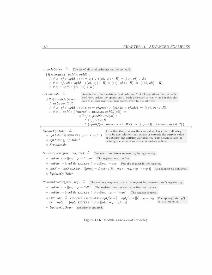
180 CHAPTER 11. ADVANCED EXAMPLES
totalOpOrder ∆= The set of all total orderings on the set opId .
{R ∈ subset (opId × opId) :∧ ∀ oi , oj ∈ opId : (oi = oj ) ∨ (〈oi , oj 〉 ∈ R) ∨ (〈oj , oi 〉 ∈ R)∧ ∀ oi , oj , ok ∈ opId : (〈oi , oj 〉 ∈ R) ∧ (〈oj , ok 〉 ∈ R) ⇒ (〈oi , ok 〉 ∈ R)∧ ∀ oi ∈ opId : 〈oi , oi 〉 /∈ R }
Serializable ∆= Asserts that there exists a total ordering R of all operations that extendsopOrder , orders the operations of each processor correctly, and makes thesource of each read the most recent write to the address.
∃R ∈ totalOpOrder :∧ opOrder ⊆ R∧ ∀ oi , oj ∈ opId : (oi .proc = oj .proc) ∧ (oi .idx < oj .idx ) ⇒ (〈oi , oj 〉 ∈ R)∧ ∀ oi ∈ opId : (“source” ∈ domain opIdQ(oi)) ⇒
¬ (∃ oj ∈ goodSource(oi) :∧ 〈oj , oi 〉 ∈ R∧ (opIdQ(oi).source 6= InitWr) ⇒ (〈opIdQ(oi).source, oj 〉 ∈ R) )
UpdateOpOrder ∆=∧ opOrder ′ ∈ subset (opId ′ × opId ′)∧ opOrder ⊆ opOrder ′
∧ Serializable′
An action that chooses the new value of opOrder , allowingit to be any relation that equals or extends the current valueof opOrder and satisfies Serializable. This action is used indefining the subactions of the next-state action.
IssueRequest(proc, req, reg) ∆= Processor proc issues request req in register reg .
∧ regFile[proc][reg].op = “Free” The register must be free.
∧ regFile′ = [regFile except ! [proc][reg] = req] Put the request in the register.
∧ opQ ′ = [opQ except ! [proc] = Append(@, [req 7→ req, reg 7→ reg])] Add request to opQ [proc].
∧ UpdateOpOrder
RespondToWr(proc, reg) ∆= The memory responds to a write request in processor proc’s register reg .
∧ regFile[proc][reg].op = “Wr” The register must contain an active read request.
∧ regFile′ = [regFile except ! [proc][reg].op = “Free”] The register is freed.
∧ let idx ∆= choose i ∈ domain opQ [proc] : opQ [proc][i ].reg = reg The appropriate opQentry is updated.in opQ ′ = [opQ except ! [proc][idx ].reg = Done]
∧ UpdateOpOrder opOrder is updated.
Figure 11.6: Module InnerSerial (middle).
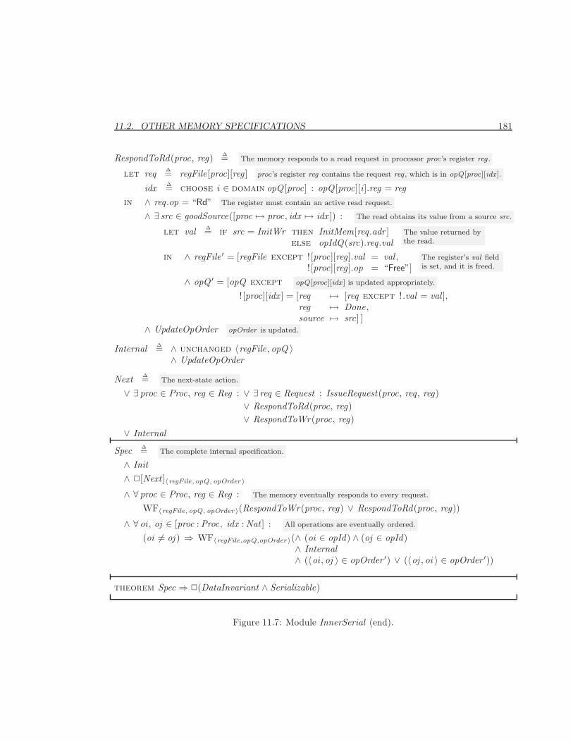
11.2. OTHER MEMORY SPECIFICATIONS 181
RespondToRd(proc, reg) ∆= The memory responds to a read request in processor proc’s register reg .
let req ∆= regFile[proc][reg] proc’s register reg contains the request req , which is in opQ [proc][idx ].
idx ∆= choose i ∈ domain opQ [proc] : opQ [proc][i ].reg = regin ∧ req.op = “Rd” The register must contain an active read request.
∧ ∃ src ∈ goodSource([proc 7→ proc, idx 7→ idx ]) : The read obtains its value from a source src.
let val ∆= if src = InitWr then InitMem[req.adr ]else opIdQ(src).req.val
The value returned bythe read.
in ∧ regFile′ = [regFile except ! [proc][reg].val = val ,! [proc][reg].op = “Free”]
The register’s val fieldis set, and it is freed.
∧ opQ ′ = [opQ except opQ [proc][idx ] is updated appropriately.
! [proc][idx ] = [req 7→ [req except !.val = val ],reg 7→ Done,source 7→ src] ]
∧ UpdateOpOrder opOrder is updated.
Internal ∆= ∧ unchanged 〈regFile, opQ 〉∧ UpdateOpOrder
Next ∆= The next-state action.
∨ ∃ proc ∈ Proc, reg ∈ Reg : ∨ ∃ req ∈ Request : IssueRequest(proc, req, reg)∨ RespondToRd(proc, reg)∨ RespondToWr(proc, reg)
∨ Internal
Spec ∆= The complete internal specification.
∧ Init∧ 2[Next ]〈regFile,opQ, opOrder 〉∧ ∀ proc ∈ Proc, reg ∈ Reg : The memory eventually responds to every request.
WF〈regFile,opQ, opOrder 〉(RespondToWr(proc, reg) ∨ RespondToRd(proc, reg))
∧ ∀ oi , oj ∈ [proc : Proc, idx : Nat ] : All operations are eventually ordered.
(oi 6= oj ) ⇒ WF〈regFile,opQ,opOrder 〉(∧ (oi ∈ opId) ∧ (oj ∈ opId)∧ Internal∧ (〈oi , oj 〉 ∈ opOrder ′) ∨ (〈oj , oi 〉 ∈ opOrder ′))
theorem Spec ⇒ 2(DataInvariant ∧ Serializable)
Figure 11.7: Module InnerSerial (end).
182 CHAPTER 11. ADVANCED EXAMPLES
The order in which operations are removed from opQ is an explanatory executionorder that satisfies requirement 1 if the Internal action satisfies these properties:
• Only completed operations are removed from opQ .3
• When a write of value val to address adr is removed from opQ , the valueof mem[adr ] is set to val .
• A read of address adr that returned a value val can be removed from opQonly if mem[adr ] = val .
Requirement 2 is satisfied if operations issued by processor p are added by theIssueRequest action to the tail of opQ [p], and are removed by the Internal actiononly from the head of opQ [p].
We have now determined what the IssueRequest and Internal actions shoulddo. The RespondToWr action is obvious; it’s essentially the same as in the serialmemory specification. The problem is the RespondToRd action. How can wedefine it so that the value returned by a read is one that mem will contain whenthe Internal action has to remove the read from opQ? The answer is surprisinglysimple: we allow the read to return any value. If the read were to return a badvalue—for example, one that is never written—then the Internal action wouldnever be able to remove the read from opQ . We rule out that possibility with aliveness condition requiring that every operation in opQ eventually is removed.This makes it easy to write the Internal action. The only remaining problem isexpressing the liveness condition.
To guarantee that every operation is eventually removed from opQ , it suf-fices to guarantee that, for every processor Proc, the operation at the head ofopQ [proc] is eventually removed. The desired liveness condition can thereforebe expressed as:
∀ proc ∈ PRoc : WF〈 ...〉(RemoveOp(proc))
where RemoveOp(proc) is an action that unconditionally removes the operationfrom the head of opQ [proc]. For convenience, we let the RemoveOp(proc) actionalso update mem. We then define a separate action Internal(proc) for eachprocessor proc. It conjoins to RemoveOp(proc) the following enabling condition,which asserts that if the operation being removed is a read, then it has returnedthe correct value.
(Head(opQ [proc]).req.op = “Rd”)⇒(mem[Head(opQ [proc]).req.adr ] = Head(opQ [proc]).req.val)
The complete internal specification, with the variables opQ and mem visible,appears in module InnerSequential on pages 184–185. At this point, you should
3We could allow uncompleted writes to be removed, but that would complicate the speci-fication.
11.2. OTHER MEMORY SPECIFICATIONS 183
have no trouble understanding it. You should also have no trouble writing amodule that instantiates InnerSequential and hides the internal variables opQand mem to produce the final specification, so I won’t bother doing it for you.
11.2.5 The Memory Specifications Considered
Almost every specification we write admits a direct implementation, based onthe initial predicate and next-state action. Such an implementation may becompletely impractical, but it is theoretically possible. It’s easy to implementthe linearizable memory with a single central memory. A direct implementationof the serial memory would require maintaining queues of all operations issuedthus far, and a computationally infeasible search for possible total orderings.But, in theory, it’s easy.
Our specification of a sequentially consistent memory cannot be directly im-plemented. A direct implementation would have to guess the correct value toreturn on a read, which is impossible. The specification is not directly imple-mentable because it is not machine closed. As explained in Section 8.7.2 onpage 100, a non-machine closed specification is one in which a direct implemen-tation can “paint itself into a corner,” reaching a point at which it is no longerpossible to satisfy the specification. Any finite scenario of memory operationscan be produced by a behavior satisfying the sequentially consistent memory’sinitial predicate and next-state action—namely, a behavior that contains noInternal steps. However, not every finite scenario can be extended to one thatis explainable by a sequential execution. For example, no scenario that beginsas follows is possible in a two-processor system: This notation for
describing scenar-ios was introducedon page 170.
Processor p : Wrp(a1, v1), Rdp(a1, v2), Wrp(a2, v2)Processor q : Wrq(a2, v1), Rdq(a2, v2), Wrq(a1, v2)
Here’s why:
Wrq(a1, v2)precedes Rdp(a1, v2) This is the only explanation of the value read by p.
precedes Wrp(a2, v2) By the order in which operations are issued.
precedes Rdq(a2, v2) This is the only explanation of the value read by q .
precedes Wrq(a1, v2) By the order in which operations are issued.
Hence q’s write of a1 must precede itself, which is impossible.As mentioned in Section 8.7.2, a specification is machine closed if the liveness
property is the conjunction of fairness properties for actions that imply thenext-state action. The sequential memory specification asserts weak fairness ofRemoveOp(proc), for processors proc, and RemoveOp(proc) does not imply thenext-state action. (The next-state action does not allow a RemoveOp(proc) stepthat removes from opQ [proc] a read that has returned the wrong value.)
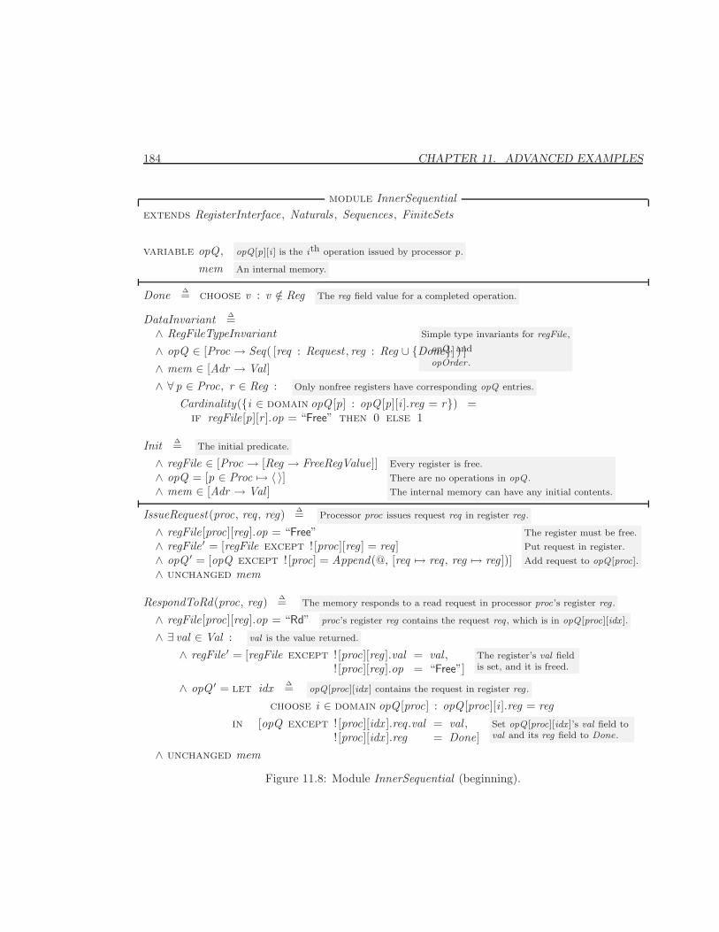
184 CHAPTER 11. ADVANCED EXAMPLES
module InnerSequentialextends RegisterInterface, Naturals , Sequences , FiniteSets
variable opQ , opQ [p][i ] is the ith operation issued by processor p.
mem An internal memory.
Done ∆= choose v : v /∈ Reg The reg field value for a completed operation.
DataInvariant ∆=∧ RegFileTypeInvariant Simple type invariants for regFile,
opQ , and
opOrder .∧ opQ ∈ [Proc → Seq( [req : Request , reg : Reg ∪ {Done}] ) ]∧ mem ∈ [Adr → Val ]∧ ∀ p ∈ Proc, r ∈ Reg : Only nonfree registers have corresponding opQ entries.
Cardinality({i ∈ domain opQ [p] : opQ [p][i ].reg = r}) =if regFile[p][r ].op = “Free” then 0 else 1
Init ∆= The initial predicate.
∧ regFile ∈ [Proc → [Reg → FreeRegValue]]∧ opQ = [p ∈ Proc 7→ 〈 〉]∧ mem ∈ [Adr → Val ]
Every register is free.
There are no operations in opQ .
The internal memory can have any initial contents.
IssueRequest(proc, req, reg) ∆= Processor proc issues request req in register reg .
∧ regFile[proc][reg].op = “Free”∧ regFile′ = [regFile except ! [proc][reg] = req]∧ opQ ′ = [opQ except ! [proc] = Append(@, [req 7→ req, reg 7→ reg])]∧ unchanged mem
The register must be free.
Put request in register.
Add request to opQ [proc].
RespondToRd(proc, reg) ∆= The memory responds to a read request in processor proc’s register reg .
∧ regFile[proc][reg].op = “Rd” proc’s register reg contains the request req , which is in opQ [proc][idx ].
∧ ∃ val ∈ Val : val is the value returned.
∧ regFile′ = [regFile except ! [proc][reg].val = val ,! [proc][reg].op = “Free”]
The register’s val fieldis set, and it is freed.
∧ opQ ′ = let idx ∆= opQ [proc][idx ] contains the request in register reg .
choose i ∈ domain opQ [proc] : opQ [proc][i ].reg = regin [opQ except ! [proc][idx ].req.val = val ,
! [proc][idx ].reg = Done]Set opQ [proc][idx ]’s val field toval and its reg field to Done.
∧ unchanged mem
Figure 11.8: Module InnerSequential (beginning).
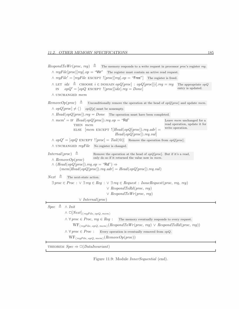
11.2. OTHER MEMORY SPECIFICATIONS 185
RespondToWr(proc, reg) ∆= The memory responds to a write request in processor proc’s register reg .
∧ regFile[proc][reg].op = “Wr” The register must contain an active read request.
∧ regFile′ = [regFile except ! [proc][reg].op = “Free”] The register is freed.
∧ let idx ∆= choose i ∈ domain opQ [proc] : opQ [proc][i ].reg = reg The appropriate opQentry is updated.in opQ ′ = [opQ except ! [proc][idx ].reg = Done]
∧ unchanged mem
RemoveOp(proc) ∆= Unconditionally remove the operation at the head of opQ [proc] and update mem.
∧ opQ [proc] 6= 〈 〉 opQ [p] must be nonempty.
∧ Head(opQ [proc]).reg = Done The operation must have been completed.
∧ mem ′ = if Head(opQ [proc]).req.op = “Rd”then memelse [mem except ! [Head(opQ [proc]).req.adr ] =
Head(opQ [proc]).req.val ]
Leave mem unchanged for aread operation, update it forwrite operation.
∧ opQ ′ = [opQ except ! [proc] = Tail(@)] Remove the operation from opQ [proc].
∧ unchanged regFile No register is changed.
Internal(proc) ∆= Remove the operation at the head of opQ [proc]. But if it’s a read,only do so if it returned the value now in mem.∧ RemoveOp(proc)
∧ (Head(opQ [proc]).req.op = “Rd”)⇒(mem[Head(opQ [proc]).req.adr ] = Head(opQ [proc]).req.val)
Next ∆= The next-state action.
∃ proc ∈ Proc : ∨ ∃ reg ∈ Reg : ∨ ∃ req ∈ Request : IssueRequest(proc, req, reg)∨ RespondToRd(proc, reg)∨ RespondToWr(proc, reg)
∨ Internal(proc)
Spec ∆= ∧ Init∧ 2[Next ]〈regFile,opQ, mem 〉∧ ∀ proc ∈ Proc, reg ∈ Reg : The memory eventually responds to every request.
WF〈regFile,opQ, mem 〉(RespondToWr(proc, reg) ∨ RespondToRd(proc, reg))
∧ ∀ proc ∈ Proc : Every operation is eventually removed from opQ .
WF〈regFile,opQ, mem 〉(RemoveOp(proc))
theorem Spec ⇒ 2(DataInvariant)
Figure 11.9: Module InnerSequential (end).
186 CHAPTER 11. ADVANCED EXAMPLES
Very high-level system specifications, such as our memory specifications aresubtle. It’s easy to get them wrong. The approach we used in the serial mem-ory specification—namely, writing conditions on the history of all operations—isdangerous. It’s easy to forget some conditions. A non-machine closed specifica-tion can occasionally be the simplest way to express what you want so say.

Part III
The Tools
187

Chapter 12
The Java Front End
The Java Front End is a parser for TLA+ written in Java by Jean-CharlesGregoire. It provides a front end for other tools, such as TLC (see Chapter 13).It can also be run by itself to find syntax errors in a specification. You shouldobtain directions for running the Java Front End’s parser on your particularsystem when you obtain the software.
12.1 Finding an Error
When the parser reports an error, finding what caused it can be tricky. Theerrors that the parser detects fall into two separate classes, which are usuallycalled syntactic and semantic errors. A syntax error is one that makes the spec-ification grammatically incorrect, meaning that it violates the BNF grammar,or the precedence and alignment rules, described in Chapter 14. A semanticerror is one that violates the legality conditions mentioned in Chapter 16. Theterm semantic error is misleading, because it suggests an error that makes aspecification have the wrong meaning. All errors found by the parser are onesthat make the specification illegal—that is, not syntactically well-formed—andhence make it have no meaning at all.
The parser reads the file sequentially, starting from the beginning, and itreports a syntax error if and when it reaches a point at which it becomes impos-sible for any continuation to produce a grammatically correct specification. Forexample, if you leave out a colon and type \A x P(x) instead of \A x : P(x),the parser will print something like:
Encountered "P" at line 7, column 11.Was expecting one of:
"," ...<OpSymbol> ...
189
190 CHAPTER 12. THE JAVA FRONT END
":" ...
The “was expecting” list describes every possible symbol that could lead to agrammatically correct specification. Knowing what the parser was expectingcan sometimes help find the error.
The parser may detect a grammatical error far from the actual mistake. Forexample, suppose you type [ instead of { to produce [x ∈ . . . : P(x )}, where “. . .”is a very long expression. The parser will discover the error only when it seesthe colon, well past the erroneous [. If you can’t find the source of an error, trythe “divide and conquer” method: keep removing different parts of the moduleuntil you isolate the source of the problem.
A typical semantic error is an undefined symbol that arises because youmistype an identifier. For example, if you define an operator Cat but spell itcat somewhere by mistake, the parser may report
unresolved identifier cat at [line: 87, col: 6] to [87,8].
The source of a semantic error is usually easy to find.The parser stops when it encounters the first syntactic error. It can detect
multiple semantic errors in a single run.The current version of the parser has the following limitations, which should
be corrected in future versions:
• It does not detect certain semantic errors. In particular, it does not doany level checking. (See Section 16.2 on page 295.)
• It does not properly handle strings with “escape sequences” such as \".(See Section 15.1.10.)
• It does not properly handle parametrized instantiation. (See Section 4.2.2on page 39.)
• It does not handle the symbol (\X). You must type \otimes to represent⊗.
• It produces meaningless warnings of the form
numbers are used but NUMERAL isn’t defined
This warning is a remnant of a minor change to TLA+.
• It does not handle numbers written in binary, octal, or hexadecimal nota-tion. (See Section 15.1.11.)
Chapter 13
The TLC Model Checker
This is a description of how we expect Version 2.0 of TLC to behave. Version 1.0of TLC does not completely implement this description; Section 13.4 on page 221describes its limitations. Section 13.5 on page 223 describes improvements thatwe may make to later versions.
13.1 Introduction to TLC
TLC is a program for finding errors in TLA+ specifications. A syntacticallycorrect specification can have two kinds of errors: it may contain “silliness” orit may not capture the intention of its author. As explained in Section 6.2,a silly expression is one whose meaning is not determined by the semantics ofTLA+—for example, 3 + 〈1, 2〉. A specification is incorrect if whether or notsome particular behavior satisfies it depends on the meaning of a silly expression.Intention isn’t a well-defined concept, and there may be a fine line between errorsand unintended features.
Experience has shown that one of the most effective ways of finding bothkinds of errors is by trying to verify invariance properties of a specification. TLCtries to find errors by looking for counterexamples to invariance properties—thatis, to assertions of the form
Init ∧ 2[Next ]v ⇒ 2Inv(13.1)
where Inv is a state predicate. One example of an invariance property is theabsence of deadlock, in which Inv equals Enabled Next . A counterexampleto this instance of (13.1) shows the possibility of deadlock—the ability of thesystem to reach a state in which no further progress is possible. (Of course, forsome systems, deadlock may just mean successful termination.) As explained inSections 13.3.4 and 13.3.5 below, TLC can also be used to check other propertiesbesides invariance.
191
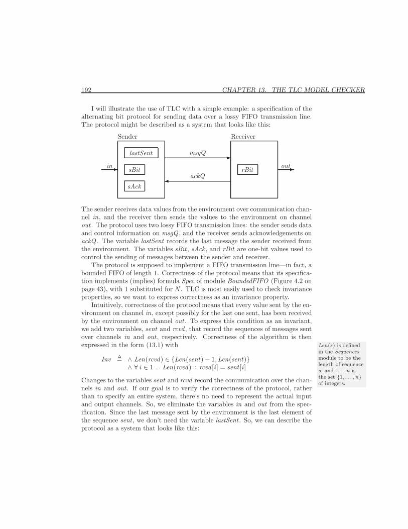
192 CHAPTER 13. THE TLC MODEL CHECKER
I will illustrate the use of TLC with a simple example: a specification of thealternating bit protocol for sending data over a lossy FIFO transmission line.The protocol might be described as a system that looks like this:
Sender
lastSent
sBit
sAck
Receiver
rBitin-
msgQ -
ackQ�
-out
The sender receives data values from the environment over communication chan-nel in, and the receiver then sends the values to the environment on channelout . The protocol uses two lossy FIFO transmission lines: the sender sends dataand control information on msgQ , and the receiver sends acknowledgements onackQ . The variable lastSent records the last message the sender received fromthe environment. The variables sBit , sAck , and rBit are one-bit values used tocontrol the sending of messages between the sender and receiver.
The protocol is supposed to implement a FIFO transmission line—in fact, abounded FIFO of length 1. Correctness of the protocol means that its specifica-tion implements (implies) formula Spec of module BoundedFIFO (Figure 4.2 onpage 43), with 1 substituted for N . TLC is most easily used to check invarianceproperties, so we want to express correctness as an invariance property.
Intuitively, correctness of the protocol means that every value sent by the en-vironment on channel in, except possibly for the last one sent, has been receivedby the environment on channel out . To express this condition as an invariant,we add two variables, sent and rcvd , that record the sequences of messages sentover channels in and out , respectively. Correctness of the algorithm is thenexpressed in the form (13.1) with Len(s) is defined
in the Sequencesmodule to be thelength of sequences, and 1 . . n isthe set {1, . . . ,n}of integers.
Inv ∆= ∧ Len(rcvd) ∈ {Len(sent)− 1,Len(sent)}∧ ∀ i ∈ 1 . . Len(rcvd) : rcvd [i ] = sent [i ]
Changes to the variables sent and rcvd record the communication over the chan-nels in and out . If our goal is to verify the correctness of the protocol, ratherthan to specify an entire system, there’s no need to represent the actual inputand output channels. So, we eliminate the variables in and out from the spec-ification. Since the last message sent by the environment is the last element ofthe sequence sent , we don’t need the variable lastSent . So, we can describe theprotocol as a system that looks like this:
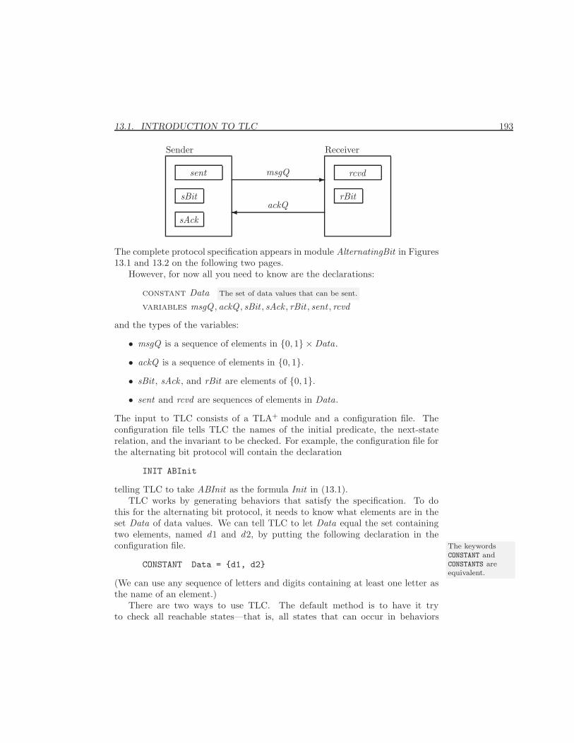
13.1. INTRODUCTION TO TLC 193
Sender
sent
sBit
sAck
Receiver
rcvd
rBit
msgQ -
ackQ�
The complete protocol specification appears in module AlternatingBit in Figures13.1 and 13.2 on the following two pages.
However, for now all you need to know are the declarations:
constant Data The set of data values that can be sent.
variables msgQ , ackQ , sBit , sAck , rBit , sent , rcvd
and the types of the variables:
• msgQ is a sequence of elements in {0, 1} ×Data.
• ackQ is a sequence of elements in {0, 1}.• sBit , sAck , and rBit are elements of {0, 1}.• sent and rcvd are sequences of elements in Data.
The input to TLC consists of a TLA+ module and a configuration file. Theconfiguration file tells TLC the names of the initial predicate, the next-staterelation, and the invariant to be checked. For example, the configuration file forthe alternating bit protocol will contain the declaration
INIT ABInit
telling TLC to take ABInit as the formula Init in (13.1).TLC works by generating behaviors that satisfy the specification. To do
this for the alternating bit protocol, it needs to know what elements are in theset Data of data values. We can tell TLC to let Data equal the set containingtwo elements, named d1 and d2, by putting the following declaration in theconfiguration file. The keywords
CONSTANT andCONSTANTS areequivalent.
CONSTANT Data = {d1, d2}
(We can use any sequence of letters and digits containing at least one letter asthe name of an element.)
There are two ways to use TLC. The default method is to have it tryto check all reachable states—that is, all states that can occur in behaviors
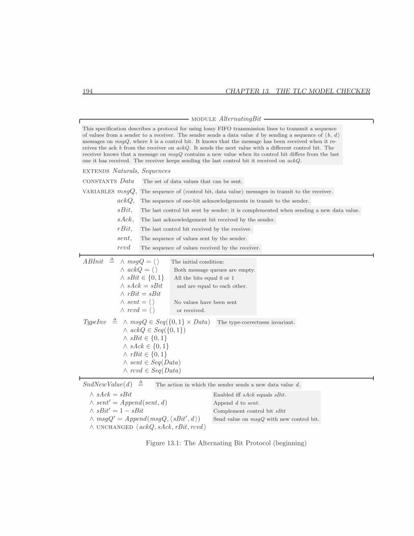
194 CHAPTER 13. THE TLC MODEL CHECKER
module AlternatingBitThis specification describes a protocol for using lossy FIFO transmission lines to transmit a sequenceof values from a sender to a receiver. The sender sends a data value d by sending a sequence of 〈b, d 〉messages on msgQ , where b is a control bit. It knows that the message has been received when it re-ceives the ack b from the receiver on ackQ . It sends the next value with a different control bit. Thereceiver knows that a message on msgQ contains a new value when its control bit differs from the lastone it has received. The receiver keeps sending the last control bit it received on ackQ .
extends Naturals, Sequencesconstants Data The set of data values that can be sent.
variables msgQ, The sequence of 〈control bit, data value〉 messages in transit to the receiver.
ackQ, The sequence of one-bit acknowledgements in transit to the sender.
sBit, The last control bit sent by sender; it is complemented when sending a new data value.
sAck, The last acknowledgement bit received by the sender.
rBit, The last control bit received by the receiver.
sent, The sequence of values sent by the sender.
rcvd The sequence of values received by the receiver.
ABInit ∆= ∧ msgQ = 〈 〉∧ ackQ = 〈 〉∧ sBit ∈ {0, 1}∧ sAck = sBit∧ rBit = sBit∧ sent = 〈 〉∧ rcvd = 〈 〉
The initial condition:
Both message queues are empty.
All the bits equal 0 or 1
and are equal to each other.
No values have been sent
or received.
TypeInv ∆= ∧ msgQ ∈ Seq({0, 1} ×Data)∧ ackQ ∈ Seq({0, 1})∧ sBit ∈ {0, 1}∧ sAck ∈ {0, 1}∧ rBit ∈ {0, 1}∧ sent ∈ Seq(Data)∧ rcvd ∈ Seq(Data)
The type-correctness invariant.
SndNewValue(d) ∆= The action in which the sender sends a new data value d .
∧ sAck = sBit∧ sent ′ = Append(sent , d)∧ sBit ′ = 1− sBit∧ msgQ ′ = Append(msgQ , 〈sBit ′, d 〉)∧ unchanged 〈ackQ , sAck , rBit , rcvd 〉
Enabled iff sAck equals sBit .
Append d to sent .
Complement control bit sBit
Send value on msgQ with new control bit.
Figure 13.1: The Alternating Bit Protocol (beginning)
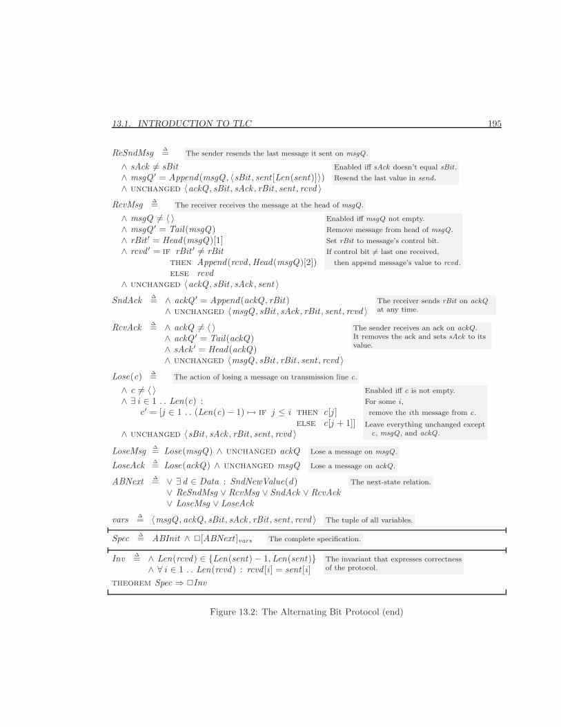
13.1. INTRODUCTION TO TLC 195
ReSndMsg ∆= The sender resends the last message it sent on msgQ .
∧ sAck 6= sBit∧ msgQ ′ = Append(msgQ , 〈sBit , sent [Len(sent)]〉)∧ unchanged 〈ackQ , sBit , sAck , rBit , sent , rcvd 〉
Enabled iff sAck doesn’t equal sBit .
Resend the last value in send .
RcvMsg ∆= The receiver receives the message at the head of msgQ .
∧ msgQ 6= 〈 〉∧ msgQ ′ = Tail(msgQ)∧ rBit ′ = Head(msgQ)[1]∧ rcvd ′ = if rBit ′ 6= rBit
then Append(rcvd ,Head(msgQ)[2])else rcvd
∧ unchanged 〈ackQ , sBit , sAck , sent 〉
Enabled iff msgQ not empty.
Remove message from head of msgQ .
Set rBit to message’s control bit.
If control bit 6= last one received,
then append message’s value to rcvd .
SndAck ∆= ∧ ackQ ′ = Append(ackQ , rBit)∧ unchanged 〈msgQ , sBit , sAck , rBit , sent , rcvd 〉
The receiver sends rBit on ackQat any time.
RcvAck ∆= ∧ ackQ 6= 〈 〉∧ ackQ ′ = Tail(ackQ)∧ sAck ′ = Head(ackQ)∧ unchanged 〈msgQ , sBit , rBit , sent , rcvd 〉
The sender receives an ack on ackQ .It removes the ack and sets sAck to itsvalue.
Lose(c) ∆= The action of losing a message on transmission line c.
∧ c 6= 〈 〉∧ ∃ i ∈ 1 . . Len(c) :
c′ = [j ∈ 1 . . (Len(c)− 1) 7→ if j ≤ i then c[j ]else c[j + 1]]
∧ unchanged 〈sBit , sAck , rBit , sent , rcvd 〉
Enabled iff c is not empty.
For some i ,
remove the ith message from c.
Leave everything unchanged exceptc, msgQ , and ackQ .
LoseMsg ∆= Lose(msgQ) ∧ unchanged ackQ Lose a message on msgQ .
LoseAck ∆= Lose(ackQ) ∧ unchanged msgQ Lose a message on ackQ .
ABNext ∆= ∨ ∃ d ∈ Data : SndNewValue(d)∨ ReSndMsg ∨ RcvMsg ∨ SndAck ∨ RcvAck∨ LoseMsg ∨ LoseAck
The next-state relation.
vars ∆= 〈msgQ , ackQ , sBit , sAck , rBit , sent , rcvd 〉 The tuple of all variables.
Spec ∆= ABInit ∧ 2[ABNext ]vars The complete specification.
Inv ∆= ∧ Len(rcvd) ∈ {Len(sent)− 1,Len(sent)}∧ ∀ i ∈ 1 . . Len(rcvd) : rcvd [i ] = sent [i ]
The invariant that expresses correctnessof the protocol.
theorem Spec ⇒ 2Inv
Figure 13.2: The Alternating Bit Protocol (end)
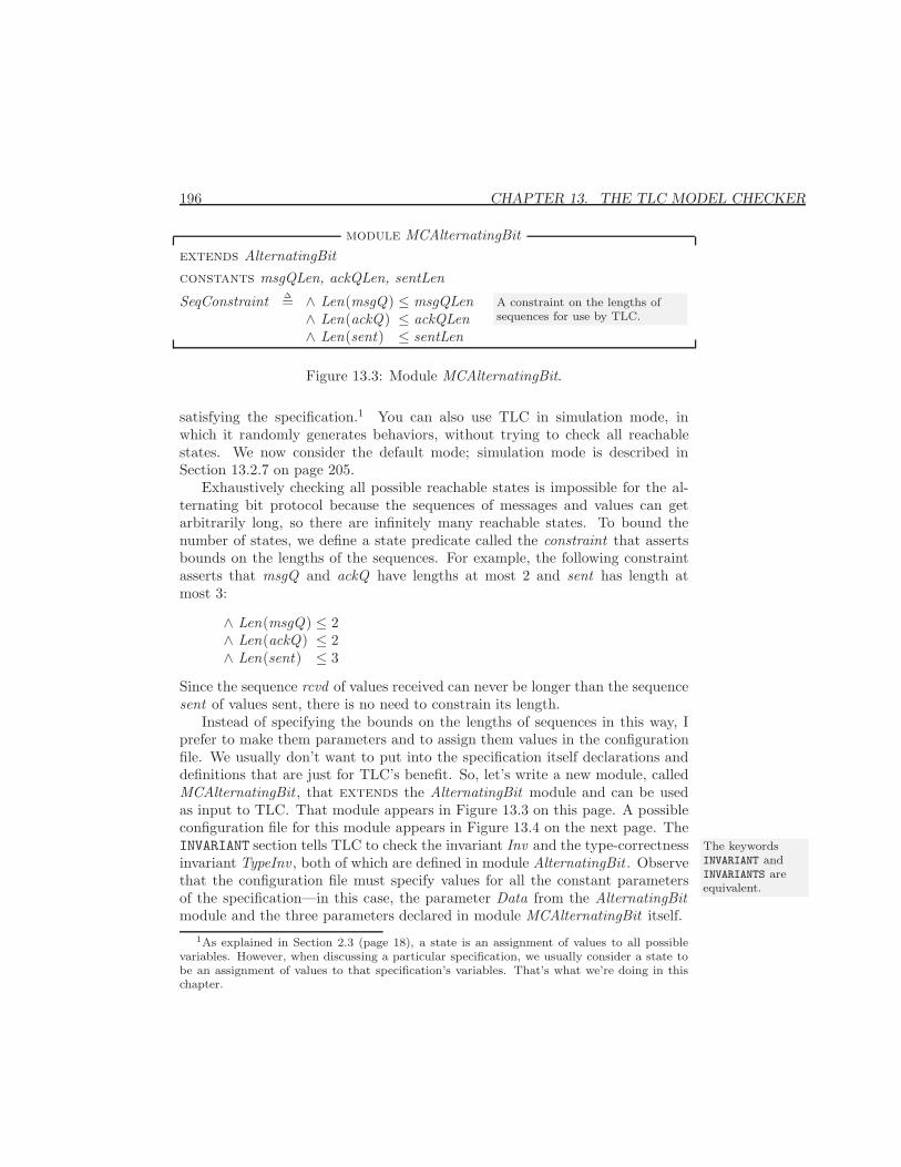
196 CHAPTER 13. THE TLC MODEL CHECKER
module MCAlternatingBitextends AlternatingBitconstants msgQLen, ackQLen, sentLen
SeqConstraint ∆= ∧ Len(msgQ) ≤ msgQLen∧ Len(ackQ) ≤ ackQLen∧ Len(sent) ≤ sentLen
A constraint on the lengths ofsequences for use by TLC.
Figure 13.3: Module MCAlternatingBit.
satisfying the specification.1 You can also use TLC in simulation mode, inwhich it randomly generates behaviors, without trying to check all reachablestates. We now consider the default mode; simulation mode is described inSection 13.2.7 on page 205.
Exhaustively checking all possible reachable states is impossible for the al-ternating bit protocol because the sequences of messages and values can getarbitrarily long, so there are infinitely many reachable states. To bound thenumber of states, we define a state predicate called the constraint that assertsbounds on the lengths of the sequences. For example, the following constraintasserts that msgQ and ackQ have lengths at most 2 and sent has length atmost 3:
∧ Len(msgQ) ≤ 2∧ Len(ackQ) ≤ 2∧ Len(sent) ≤ 3
Since the sequence rcvd of values received can never be longer than the sequencesent of values sent, there is no need to constrain its length.
Instead of specifying the bounds on the lengths of sequences in this way, Iprefer to make them parameters and to assign them values in the configurationfile. We usually don’t want to put into the specification itself declarations anddefinitions that are just for TLC’s benefit. So, let’s write a new module, calledMCAlternatingBit , that extends the AlternatingBit module and can be usedas input to TLC. That module appears in Figure 13.3 on this page. A possibleconfiguration file for this module appears in Figure 13.4 on the next page. TheINVARIANT section tells TLC to check the invariant Inv and the type-correctness The keywords
INVARIANT andINVARIANTS areequivalent.
invariant TypeInv , both of which are defined in module AlternatingBit . Observethat the configuration file must specify values for all the constant parametersof the specification—in this case, the parameter Data from the AlternatingBitmodule and the three parameters declared in module MCAlternatingBit itself.
1As explained in Section 2.3 (page 18), a state is an assignment of values to all possiblevariables. However, when discussing a particular specification, we usually consider a state tobe an assignment of values to that specification’s variables. That’s what we’re doing in thischapter.
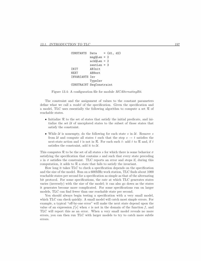
13.1. INTRODUCTION TO TLC 197
CONSTANTS Data = {d1, d2}msgQLen = 2ackQLen = 2sentLen = 3
INIT ABInitNEXT ABNextINVARIANTS Inv
TypeInvCONSTRAINT SeqConstraint
Figure 13.4: A configuration file for module MCAlternatingBit.
The constraint and the assignment of values to the constant parametersdefine what we call a model of the specification. Given the specification anda model, TLC uses essentially the following algorithm to compute a set R ofreachable states.
• Initialize R to the set of states that satisfy the initial predicate, and ini-tialize the set U of unexplored states to the subset of those states thatsatisfy the constraint.
• While U is nonempty, do the following for each state s in U . Remove sfrom U and compute all states t such that the step s → t satisfies thenext-state action and t is not in R. For each such t : add t to R and, if tsatisfies the constraint, add it to U .
This computes R to be the set of all states s for which there is some behavior σsatisfying the specification that contains s and such that every state precedings in σ satisfies the constraint. TLC reports an error and stops if, during thiscomputation, it adds to R a state that fails to satisfy the invariant.
How long it takes TLC to check a specification depends on the specificationand the size of the model. Run on a 600MHz work station, TLC finds about 1000reachable states per second for a specification as simple as that of the alternatingbit protocol. For some specifications, the rate at which TLC generates statesvaries (inversely) with the size of the model; it can also go down as the statesit generates become more complicated. For some specifications run on largermodels, TLC can find fewer than one reachable state per second.
You should always begin testing a specification with a very small model,which TLC can check quickly. A small model will catch most simple errors. Forexample, a typical “off-by-one error” will make the next state depend upon thevalue of an expression f [e] when e is not in the domain of the function f , andTLC will report this as an error. When a very small model reveals no moreerrors, you can then run TLC with larger models to try to catch more subtleerrors.
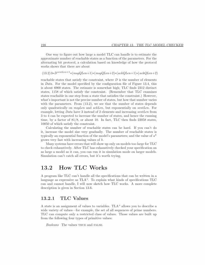
198 CHAPTER 13. THE TLC MODEL CHECKER
One way to figure out how large a model TLC can handle is to estimate theapproximate number of reachable states as a function of the parameters. For thealternating bit protocol, a calculation based on knowledge of how the protocolworks shows that there are about
3∗DsentLen+1∗(msgQLen+1)∗(msgQLen+2)∗(ackQLen+1)∗(ackQLen+2)(13.2)
reachable states that satisfy the constraint, where D is the number of elementsin Data. For the model specified by the configuration file of Figure 13.4, thisis about 6900 states. The estimate is somewhat high; TLC finds 2312 distinctstates, 1158 of which satisfy the constraint. (Remember that TLC examinesstates reachable in one step from a state that satisfies the constraint.) However,what’s important is not the precise number of states, but how that number varieswith the parameters. From (13.2), we see that the number of states dependsonly quadratically on msgLen and ackLen, but exponentially on sentLen. Forexample, letting Data have 3 instead of 2 elements and increasing sentLen from3 to 4 can be expected to increase the number of states, and hence the runningtime, by a factor of 81/8, or about 10. In fact, TLC then finds 22058 states,10050 of which satisfy the constraint.
Calculating the number of reachable states can be hard. If you can’t doit, increase the model size very gradually. The number of reachable states istypically an exponential function of the model’s parameters; and the value of ab
grows very fast with increasing values of b.Many systems have errors that will show up only on models too large for TLC
to check exhaustively. After TLC has exhaustively checked your specification onas large a model as it can, you can run it in simulation mode on larger models.Simulation can’t catch all errors, but it’s worth trying.
13.2 How TLC Works
A program like TLC can’t handle all the specifications that can be written in alanguage as expressive as TLA+. To explain what kinds of specifications TLCcan and cannot handle, I will now sketch how TLC works. A more completedescription is given in Section 13.6.
13.2.1 TLC Values
A state is an assignment of values to variables. TLA+ allows you to describe awide variety of values—for example, the set of all sequences of prime numbers.TLC can compute only a restricted class of values. Those values are built upfrom the following four types of primitive values:
Booleans The values true and false.
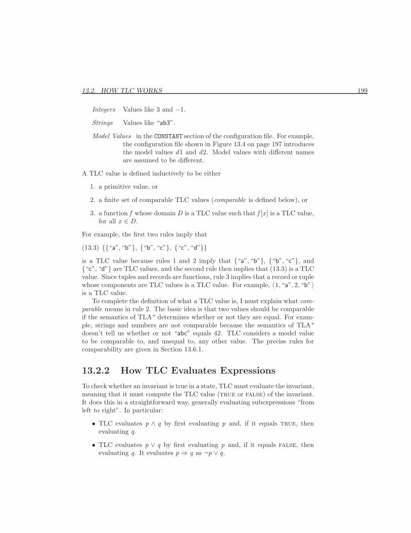
13.2. HOW TLC WORKS 199
Integers Values like 3 and −1.
Strings Values like “ab3”.
Model Values in the CONSTANT section of the configuration file. For example,the configuration file shown in Figure 13.4 on page 197 introducesthe model values d1 and d2. Model values with different namesare assumed to be different.
A TLC value is defined inductively to be either
1. a primitive value, or
2. a finite set of comparable TLC values (comparable is defined below), or
3. a function f whose domain D is a TLC value such that f [x ] is a TLC value,for all x ∈ D .
For example, the first two rules imply that
{{“a”, “b”}, {“b”, “c”}, {“c”, “d”}}(13.3)
is a TLC value because rules 1 and 2 imply that {“a”, “b”}, {“b”, “c”}, and{“c”, “d”} are TLC values, and the second rule then implies that (13.3) is a TLCvalue. Since tuples and records are functions, rule 3 implies that a record or tuplewhose components are TLC values is a TLC value. For example, 〈1, “a”, 2, “b”〉is a TLC value.
To complete the definition of what a TLC value is, I must explain what com-parable means in rule 2. The basic idea is that two values should be comparableif the semantics of TLA+ determines whether or not they are equal. For exam-ple, strings and numbers are not comparable because the semantics of TLA+
doesn’t tell us whether or not “abc” equals 42. TLC considers a model valueto be comparable to, and unequal to, any other value. The precise rules forcomparability are given in Section 13.6.1.
13.2.2 How TLC Evaluates Expressions
To check whether an invariant is true in a state, TLC must evaluate the invariant,meaning that it must compute the TLC value (true or false) of the invariant.It does this in a straightforward way, generally evaluating subexpressions “fromleft to right”. In particular:
• TLC evaluates p ∧ q by first evaluating p and, if it equals true, thenevaluating q.
• TLC evaluates p ∨ q by first evaluating p and, if it equals false, thenevaluating q. It evaluates p ⇒ q as ¬p ∨ q.
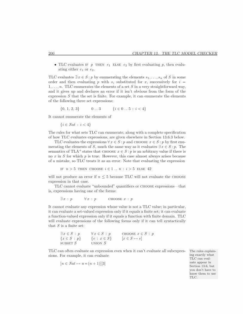
200 CHAPTER 13. THE TLC MODEL CHECKER
• TLC evaluates if p then e1 else e2 by first evaluating p, then evalu-ating either e1 or e2.
TLC evaluates ∃ x ∈ S : p by enumerating the elements s1, . . . , sn of S in someorder and then evaluating p with s i substituted for x , successively for i =1, . . . ,n. TLC enumerates the elements of a set S in a very straightforward way,and it gives up and declares an error if it isn’t obvious from the form of theexpression S that the set is finite. For example, it can enumerate the elementsof the following three set expressions:
{0, 1, 2, 3} 0 . . 3 {i ∈ 0 . . 5 : i < 4}It cannot enumerate the elements of
{i ∈ Nat : i < 4}The rules for what sets TLC can enumerate, along with a complete specificationof how TLC evaluates expressions, are given elsewhere in Section 13.6.3 below.
TLC evaluates the expressions ∀ x ∈ S : p and choose x ∈ S : p by first enu-merating the elements of S , much the same way as it evaluates ∃ x ∈ S : p. Thesemantics of TLA+ states that choose x ∈ S : p is an arbitrary value if there isno x in S for which p is true. However, this case almost always arises becauseof a mistake, so TLC treats it as an error. Note that evaluating the expression
if n > 5 then choose i ∈ 1 . . n : i > 5 else 42
will not produce an error if n ≤ 5 because TLC will not evaluate the chooseexpression in that case.
TLC cannot evaluate “unbounded” quantifiers or choose expressions—thatis, expressions having one of the forms:
∃ x : p ∀ x : p choose x : p
It cannot evaluate any expression whose value is not a TLC value; in particular,it can evaluate a set-valued expression only if it equals a finite set; it can evaluatea function-valued expression only if it equals a function with finite domain. TLCwill evaluate expressions of the following forms only if it can tell syntacticallythat S is a finite set:
∃ x ∈ S : p ∀ x ∈ S : p choose x ∈ S : p{x ∈ S : p} {e : x ∈ S} [x ∈ S 7→ e]subset S union S
TLC can often evaluate an expression even when it can’t evaluate all subexpres- The rules explain-ing exactly whatTLC can eval-uate appear inSection 13.6, butyou don’t have toknow them to useTLC.
sions. For example, it can evaluate
[n ∈ Nat 7→ n ∗ (n + 1)][3]
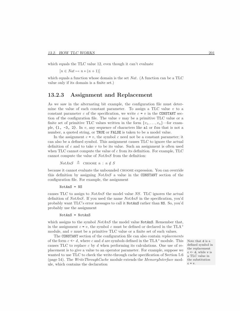
13.2. HOW TLC WORKS 201
which equals the TLC value 12, even though it can’t evaluate
[n ∈ Nat 7→ n ∗ (n + 1)]
which equals a function whose domain is the set Nat . (A function can be a TLCvalue only if its domain is a finite set.)
13.2.3 Assignment and Replacement
As we saw in the alternating bit example, the configuration file must deter-mine the value of each constant parameter. To assign a TLC value v to aconstant parameter c of the specification, we write c = v in the CONSTANT sec-tion of the configuration file. The value v may be a primitive TLC value or afinite set of primitive TLC values written in the form {v1, . . . , vn}—for exam-ple, {1, -3, 2}. In v , any sequence of characters like a1 or foo that is not anumber, a quoted string, or TRUE or FALSE is taken to be a model value.
In the assignment c = v , the symbol c need not be a constant parameter; itcan also be a defined symbol. This assignment causes TLC to ignore the actualdefinition of c and to take v to be its value. Such an assignment is often usedwhen TLC cannot compute the value of c from its definition. For example, TLCcannot compute the value of NotAnS from the definition:
NotAnS ∆= choose n : n /∈ S
because it cannot evaluate the unbounded choose expression. You can overridethis definition by assigning NotAnS a value in the CONSTANT section of theconfiguration file. For example, the assignment
NotAnS = NS
causes TLC to assign to NotAnS the model value NS . TLC ignores the actualdefinition of NotAnS . If you used the name NotAnS in the specification, you’dprobably want TLC’s error messages to call it NotAnS rather than NS. So, you’dprobably use the assignment
NotAnS = NotAnS
which assigns to the symbol NotAnS the model value NotAnS. Remember that,in the assignment c = v , the symbol c must be defined or declared in the TLA+
module, and v must be a primitive TLC value or a finite set of such values.The CONSTANT section of the configuration file can also contain replacements
of the form c <- d , where c and d are symbols defined in the TLA+module. This Note that d is adefined symbol inthe replacementc <- d, while v isa TLC value inthe substitutionc = v.
causes TLC to replace c by d when performing its calculations. One use of re-placement is to give a value to an operator parameter. For example, suppose wewanted to use TLC to check the write-through cache specification of Section 5.6(page 54). The WriteThroughCache module extends the MemoryInterface mod-ule, which contains the declaration
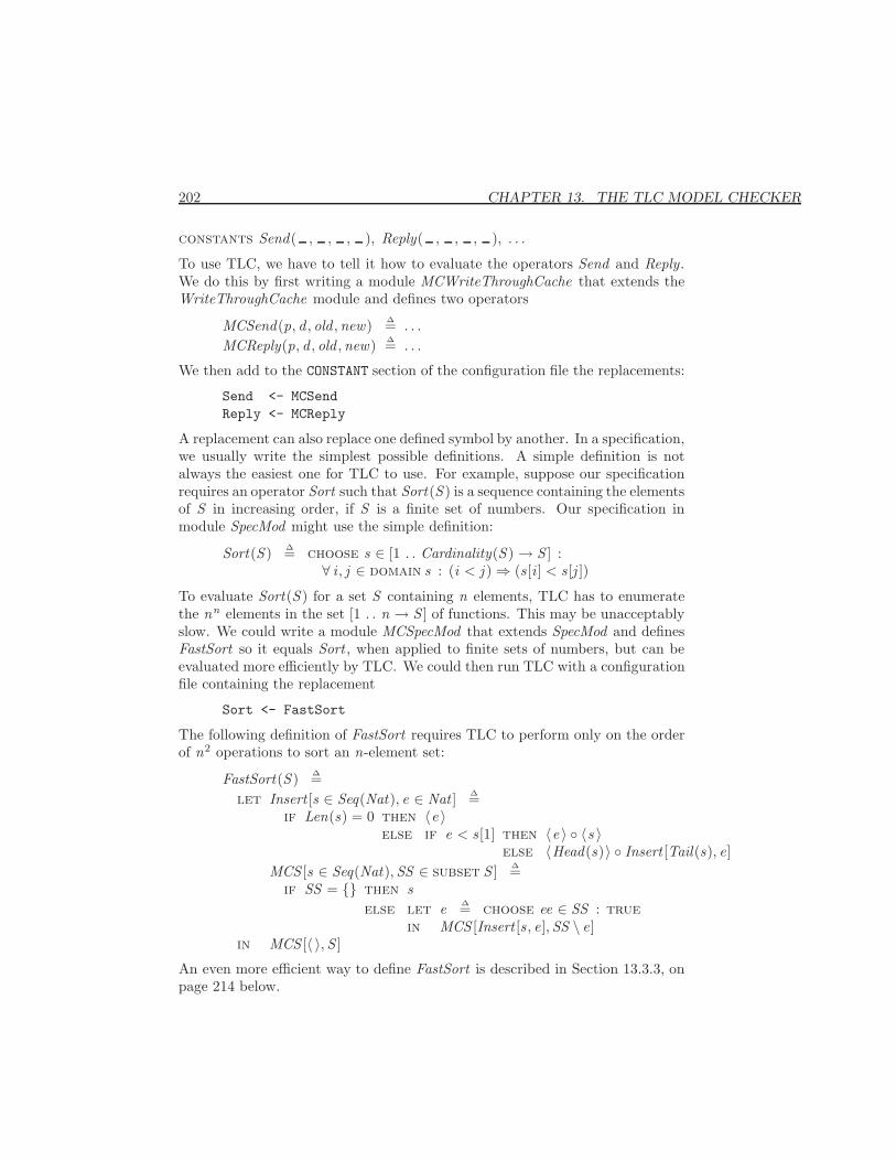
202 CHAPTER 13. THE TLC MODEL CHECKER
constants Send( , , , ), Reply( , , , ), . . .
To use TLC, we have to tell it how to evaluate the operators Send and Reply.We do this by first writing a module MCWriteThroughCache that extends theWriteThroughCache module and defines two operators
MCSend(p, d , old ,new) ∆= . . .
MCReply(p, d , old ,new) ∆= . . .
We then add to the CONSTANT section of the configuration file the replacements:
Send <- MCSendReply <- MCReply
A replacement can also replace one defined symbol by another. In a specification,we usually write the simplest possible definitions. A simple definition is notalways the easiest one for TLC to use. For example, suppose our specificationrequires an operator Sort such that Sort(S ) is a sequence containing the elementsof S in increasing order, if S is a finite set of numbers. Our specification inmodule SpecMod might use the simple definition:
Sort(S ) ∆= choose s ∈ [1 . . Cardinality(S ) → S ] :∀ i , j ∈ domain s : (i < j )⇒ (s [i ] < s [j ])
To evaluate Sort(S ) for a set S containing n elements, TLC has to enumeratethe nn elements in the set [1 . . n → S ] of functions. This may be unacceptablyslow. We could write a module MCSpecMod that extends SpecMod and definesFastSort so it equals Sort , when applied to finite sets of numbers, but can beevaluated more efficiently by TLC. We could then run TLC with a configurationfile containing the replacement
Sort <- FastSort
The following definition of FastSort requires TLC to perform only on the orderof n2 operations to sort an n-element set:
FastSort(S ) ∆=let Insert [s ∈ Seq(Nat), e ∈ Nat ] ∆=
if Len(s) = 0 then 〈e 〉else if e < s [1] then 〈e 〉 ◦ 〈s 〉
else 〈Head(s)〉 ◦ Insert [Tail(s), e]MCS [s ∈ Seq(Nat),SS ∈ subset S ] ∆=
if SS = {} then selse let e ∆= choose ee ∈ SS : true
in MCS [Insert [s , e],SS \ e]in MCS [〈 〉,S ]
An even more efficient way to define FastSort is described in Section 13.3.3, onpage 214 below.
13.2. HOW TLC WORKS 203
13.2.4 Overriding Modules
TLC cannot compute 2 + 2 from the definition of + contained in the standardNaturals module. Even if we did use a definition of + from which TLC couldcompute sums, it would not do so very quickly. Arithmetic operators like + areimplemented directly in Java, the language in which TLC is written. This isachieved by a general mechanism of TLC that allows a module to be overriddenby a Java class that implements the operators defined in the module. WhenTLC encounters an extends Naturals statement, it reads in the Java class thatoverrides the Naturals module rather than reading the module itself. Thereare Java classes to override the following standard modules: Naturals , Integers ,Sequences , FiniteSets , and Bags . (The TLC module described below in Sec-tion 13.3.3 is also overridden by a Java class.) Instructions for implementingJava classes to override other modules will appear elsewhere.
13.2.5 How TLC Computes States
When TLC evaluates the invariant, it is calculating the invariant’s value, whichis either true or false. When TLC evaluates the initial predicate or the next-state action, it is computing a set of states—the set of initial states or the setof possible successor states (primed states) for a given (unprimed) state. I willdescribe how TLC does this for the next-state relation; the evaluation of theinitial predicate is analogous.
Recall that a state is an assignment of values to variables. TLC beginscomputing the successors to a given state s by assigning to all unprimed variablestheir values in state s , and assigning no values to the primed variables. It thenstarts computing the next-state action.
TLC computes a set of successor states by simultaneously performing a setof computations, each trying to compute a single successor state. A computa-tion splits into multiple separate computations when multiple possibilities areencountered. TLC begins a single computation to evaluate the next-state rela-tion. The evaluation proceeds as described in Section 13.2.2 (page 199), exceptthat when it evaluates a subformula A ∨ B , it splits the computation into twoseparate computations—in one taking the subformula to be A and in the othertaking the subformula to be B . Similarly, when it evaluates ∃ x ∈ S : p, it splitsthe computation into multiple subcomputations, one for each element of S .
TLC reports an error if, in its evaluation, it encounters a primed variablethat is not assigned a value—except that:
• It evaluates a conjunct of the form x ′ = e when x ′ has no value by evalu-ating e and assigning to x ′ the value it obtains.
• It evaluates a conjunct of the form x ′ ∈ S as if it were ∃ v ∈ S : x ′ = v .
204 CHAPTER 13. THE TLC MODEL CHECKER
A computation that obtains the value false from evaluating the next-stateaction finds no state. A computation that obtains the value true finds thestate determined by the values assigned to the primed variables. In the lattercase, TLC reports an error if some primed variable has not been assigned avalue.
Since TLC evaluates expressions from left to right, the order in which con-juncts appear can affect whether or not TLC can evaluate the next-state action.For example, it can evaluate:
(x ′ = x + 1) ∧ (y ′ = x ′ + 1) but not (y ′ = x ′ + 1) ∧ (x ′ = x + 1)(x ′ ∈ {1, 2, 3}) ∧ (x ′ 6= x ) but not (x ′ 6= x ) ∧ (x ′ ∈ {1, 2, 3})
13.2.6 When TLC Computes What
When trying to figure out what caused an error, it helps to understand the exactorder in which TLC performs its computations. TLC executes the followingalgorithm. This algorithm depends on whether or not TLC is checking fordeadlock, which is determined by the switches with which TLC is run. (SeeSection 13.3.1.)
1. Precompute all constant definitions.
2. Compute all initial states.
3. For each initial state, evaluate the invariant on the state. If the invariantis satisfied, put the state in R; otherwise, report an error and stop.
4. Set the queue U equal to all the initial states that satisfy the constraint,arranged in some arbitrary order.
5. If the queue U is empty, stop.
6. Remove the state s from the head of U and do the following:
(a) If there is some state t such that s → t satisfies the next-state relation,then go to step 6b. If not, then if TLC is checking for deadlock, stopand report an error; otherwise go to step 5.
(b) Compute some states t such that s → t satisfies the next-state rela-tion. For each of these states t that is not in R, do the following:
i. If t does not satisfy the invariant, report an error and stop.ii. If t satisfies the constraint, add it to the end of the queue U .
(c) If there is any other state t such that s → t satisfies the next-staterelation, then go to step 6b. Otherwise, go to step 5.
TLC can use multiple threads, so step 6 may be performed concurrently bydifferent threads for different states s .
13.2. HOW TLC WORKS 205
13.2.7 Random Simulation
I have described how TLC tries to find all reachable states that satisfy a modelspecified by the configuration file. TLC can also be used in simulation modeto generate randomly chosen behaviors that satisfy the specification and checkthat they satisfy the invariant. TLC generates a behavior by randomly choosinga state s0 that satisfies the initial predicate, and then randomly choosing asequence of states s1, s2, . . . , such that each transition s i → s i+1 satisfies thenext-state action. You can specify a maximum behavior length. When TLChas generated a behavior with that many states, it starts the process again togenerate another behavior. TLC continues until it either finds an error or youstop it.
In simulation mode, there is no need to specify a constraint. (TLC ignoresit if you do.) You will probably first run TLC on models that are small enoughso it can generate all reachable states within a reasonable length of time. Whenyou have found all the errors you can in this way, you can then search for moreerrors by letting TLC generate random behaviors on larger models.
For some specifications, it can take TLC a long time to generate a transitionwhen the state gets large. For example, suppose the next-state relation containsa disjunct of the form
∧ . . .∧ T ′ ∈ subset S × S∧ Pred(T ′)
where S and T are set-valued variables and Pred is some Boolean-valued opera-tor. To choose a possible next state, TLC may have to examine all the subsets ofS × S to find a value of T ′ satisfying Pred(T ′). If S has n elements, then thereare 2n2
such subsets. You will probably want to limit the length of behaviorsgenerated by TLC to be small enough so that S cannot become too large.
TLC makes its random choices using a pseudorandom number generator.Pseudorandom number generation is controlled with a seed. Running a randomsimulation twice with the same seed produces identical results. You can eitherlet TLC choose a random seed, or specify the seed with a switch, as describedon the next page in Section 13.3.1. (TLC always prints the seed it is using.)If TLC finds an error, you can also get it to rerun just the error trace; see thedescription of the aril switch on page 207.
206 CHAPTER 13. THE TLC MODEL CHECKER
13.3 How to Use TLC
13.3.1 Running TLC
Exactly how you run TLC depends upon what operating system you are usingand how it is configured. You will probably type a command of the followingform
program name switches spec file
where:
program name is specific to your system. It might be something like java TLC.
spec file is the name of the file containing the TLA+ specification. Each TLA+
module that appears in the specification must be in a separate file namedM .tla, where M is the name of the module. The extension .tla may beomitted from spec file.
switches is a possibly empty sequence of switches. TLC accepts the followingswitches:
-config config fileSpecifies that the configuration file is named config file, which mustbe a file with extension .cfg. The extension .cfg may be omittedfrom config file. If this switch is omitted, the configuration file isassumed to have the same name as spec file, except with the extension.cfg.
-deadlockTells TLC not to check for deadlock. TLC checks for deadlock unlessthis switch is present.
-simulateTells TLC to generate randomly chosen behaviors, instead of gener-ating all reachable states. (See Section 13.2.7 above.)
-depth numThis switch tells TLC that, in simulation mode, it should generatebehaviors of length at most num. If the switch is absent, then TLCwill use a default value of 100. This switch is meaningful only whenthe -simulate switch is present.
-seed numIn simulation mode, the behaviors generated by TLC are determinedby the initial “seed” given to a pseudorandom number generator.This switch tells TLC to let the seed be num, which must be aninteger from −263 to 263−1. Running TLC twice in simulation mode
13.3. HOW TO USE TLC 207
with the same seed and aril (see the aril switch below) will produceidentical results. If this switch is omitted, TLC chooses a randomseed. This switch is meaningful only when the -simulate switch ispresent.
-aril numThe switch tells TLC that, in simulation mode, it should use num asthe aril. The aril is a modifier of the initial seed. When TLC findsan error in simulation mode, it prints out both the initial seed andan aril number. Using this initial seed and aril will cause the firsttrace generated to be that error trace. Adding Print expressions willusually not change the order in which TLC generates traces. So, ifthe trace doesn’t tell you what went wrong, you can try running TLCagain on just that trace to print out additional information.
-recover run idThis switch tells TLC to start executing the specification not fromthe beginning, but where it left off at the last checkpoint. When TLCtakes a checkpoint, it prints the run identifier. (That identifier is thesame throughout an execution of TLC.) The value of run id shouldbe that run identifier.
-cleanupTLC creates a number of files when it runs. When it completes, iterases all of them. If TLC finds an error, or if you stop it before itfinishes, TLC can leave some large files around. The -cleanup optiontells TLC to delete all files created by previous runs. Do not use thisoption if you are currently running another copy of TLC in the samedirectory; if you do, it can cause the other copy to fail.
-workers numStep 6 of the TLC execution algorithm described on page 204 canbe speeded up on a multiprocessor computer by the use of multiplethreads. This switch tells TLC to use num threads. There is neverany point to using more threads than there are actual processors onyour computer. If the switch is omitted, TLC uses a single thread.
13.3.2 Debugging a Specification
When you write a specification, it usually contains errors. The purpose of run-ning TLC is to find as many of those errors as possible. Hopefully, an error inthe specification causes TLC to report an error. The challenge of debugging isto find the error in the specification that leads to the error that TLC reports.Before addressing that problem, let’s first understand TLC’s output when itfinds no error.
208 CHAPTER 13. THE TLC MODEL CHECKER
TLC’s Normal Output
When you run TLC, the first thing it prints is the version number and creationdate—something like:
TLC Version 1.0 of 26 May 1999
Always include this information when reporting any problems with TLC. Next,TLC describes the mode in which it’s being run. The possibilities are
Model-checking
in which it is exhaustively checking all reachable states, or
Running Random Simulation with seed 1901803014088851111.
in which it is doing random simulation using the indicated seed. (See sec-tion 13.2.7.) Let’s suppose its doing model checking. TLC next types somethinglike:
Finished computing initial states:4 states generated, with 2 of them distinct.
This indicates that, when evaluating the initial predicate, TLC generated 4states, among which there were 2 distinct ones. TLC then types one or moremessages like
Progress: 2846 states generated, 984 distinct states found.856 states left on queue.
This message indicates that TLC has thus far generated and examined 2846states, it has found 984 distinct ones, and the queue U of unexplored statescontains 856 states. (See Section 13.2.6 on page 204.) After running for a while,TLC generates these progress reports about once every five minutes. For mostspecifications, the number of states on the queue increases monotonically at thebeginning of the execution and decreases monotonically at the end. The progressreports therefore provide a useful guide to how much longer the execution is likelyto take.
When TLC successfully completes, it prints
Model checking completed. No error has been found.
It then prints something like:
Estimates of the probability that TLC did not check all reachablestates because two distinct states had the same fingerprint:calculated (optimistic): .000003based on the actual fingerprints: .00007
13.3. HOW TO USE TLC 209
As explained in Section 13.6.4 on page 234, there is a chance that TLC did notexamine the complete set of reachable states. TLC prints two different estimatesof that probability. The first estimate is generally lower and more optimistic;the second is perhaps a more realistic one.
Finally, TLC prints something like
2846 transitions taken. 984 states discovered. 0 states lefton queue.
with the grand totals.While TLC is running, it may also print something like
-- Checkpointing run states/99-05-20-15-47-55 completed
This indicates that it has written a checkpoint that you can use to restart TLCin the event of a computer failure. (As explained in Section 13.3.6 on page 220,checkpoints have other uses as well.) The run identifier
states/99-05-20-15-47-55
is used with the -recover switch to restart TLC from where the checkpointwas taken. (If only part of this message was printed—for example, because yourcomputer crashed while TLC was taking the checkpoint—there is an extremelysmall chance that all the checkpoints are corrupted and you must start TLCagain from the beginning.)
Error Reports
The first problems you find in your specification will probably be syntax errors.TLC reports them with
ParseException in parseSpec:
followed by the error message generated by the parser. Chapter 12 explains howto interpret the parser’s error messages. (Note: TLC Version 1.0 does not usethe parser’s full error detection mechanism; you should check your specificationwith the parser before running TLC on it.)
After parsing, TLC executes two basic phases: in the first, it computes theinitial states and in the second it generates the successor states of states on thequeue of unexplored states. You can tell which phase TLC is in by whether ornot it has printed the “initial states computed” message.
TLC evaluates the invariant in both phases—on the initial states in the firstphase, and on newly generated successor states in the second. TLC’s moststraightforward error report occurs when the invariant is violated. Suppose weintroduce an error into our alternating bit specification (Figures 13.1 and 13.2
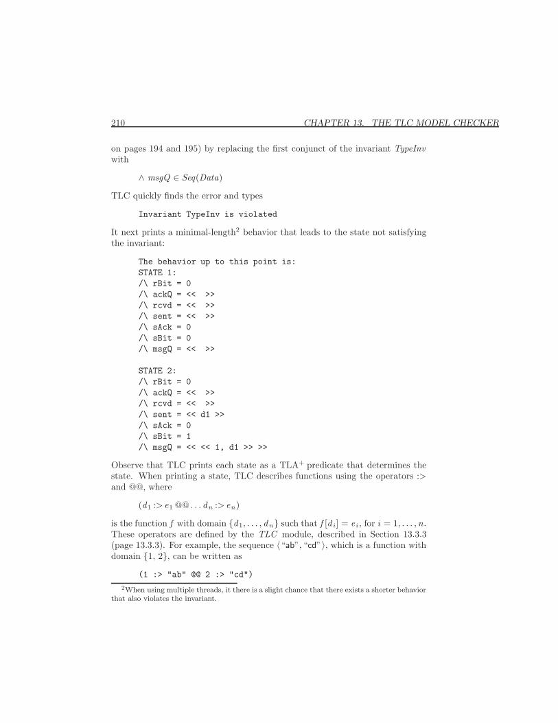
210 CHAPTER 13. THE TLC MODEL CHECKER
on pages 194 and 195) by replacing the first conjunct of the invariant TypeInvwith
∧ msgQ ∈ Seq(Data)
TLC quickly finds the error and types
Invariant TypeInv is violated
It next prints a minimal-length2 behavior that leads to the state not satisfyingthe invariant:
The behavior up to this point is:STATE 1:/\ rBit = 0/\ ackQ = << >>/\ rcvd = << >>/\ sent = << >>/\ sAck = 0/\ sBit = 0/\ msgQ = << >>
STATE 2:/\ rBit = 0/\ ackQ = << >>/\ rcvd = << >>/\ sent = << d1 >>/\ sAck = 0/\ sBit = 1/\ msgQ = << << 1, d1 >> >>
Observe that TLC prints each state as a TLA+ predicate that determines thestate. When printing a state, TLC describes functions using the operators :>and @@, where
(d1 :> e1 @@ . . . dn :> en)
is the function f with domain {d1, . . . , dn} such that f [d i ] = ei , for i = 1, . . . ,n.These operators are defined by the TLC module, described in Section 13.3.3(page 13.3.3). For example, the sequence 〈“ab”, “cd”〉, which is a function withdomain {1, 2}, can be written as
(1 :> "ab" @@ 2 :> "cd")
2When using multiple threads, it there is a slight chance that there exists a shorter behaviorthat also violates the invariant.
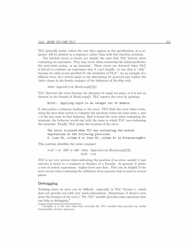
13.3. HOW TO USE TLC 211
TLC generally prints values the way they appear in the specification, so a se-quence will be printed as a sequence, rather than with this function notation.
The hardest errors to locate are usually the ones that TLC detects whenevaluating an expression. They may occur when evaluating the initial predicate,the next-state action, or an invariant. These errors are detected when TLCis forced to evaluate an expression that it can’t handle, or one that is “silly”because its value is not specified by the semantics of TLA+. As an example of asilliness error, let’s return again to the alternating bit protocol and replace thethen clause in the fourth conjunct of the definition of RcvMsg with
then Append(rcvd ,Head(msgQ)[3])
TLC discovers the error because the elements of msgQ are pairs, so 3 is not anelement in the domain of Head(msgQ). TLC reports the error by printing:
Error: Applying tuple to an integer out of domain.
It then prints a behavior leading to the error. TLC finds the error when evalu-ating the next-state action to compute the successor states for some state s , ands is the last state in that behavior. Had it found the error when evaluating theinvariant, the behavior would end with the state in which TLC was evaluatingthe invariant. Finally, TLC prints the location of the error:
The error occurred when TLC was evaluating the nestedexpressions at the following positions:0. Line 44, column 6 to line 45, column 61 in AlternatingBit
This position identifies the entire conjunct
rcvd ′ = if rBit ′ 6= rBit then Append(rcvd ,Head(msgQ)[3])else rcvd
TLC is not very precise when indicating the position of an error; usually it justnarrows it down to a conjunct or disjunct of a formula. In general, it printsa tree of nested expressions—higher-level ones first. This can be helpful if theerror occurs when evaluating the definition of an operator that is used in severalplaces.
Debugging
Tracking down an error can be difficult—especially in TLC Version 1, whichdoes not provide you with very much information. (Sometimes, it doesn’t evenprint the location of the error.) The TLC module provides some operators thatcan help in debugging.3
3Actually, it is the Java class that overrides the TLC module that provides the usefulfunctionality of these operators.
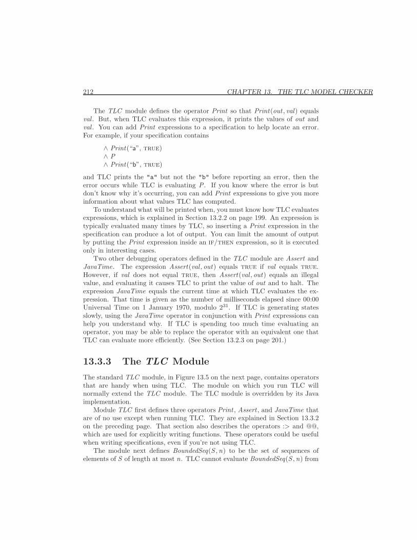
212 CHAPTER 13. THE TLC MODEL CHECKER
The TLC module defines the operator Print so that Print(out , val) equalsval . But, when TLC evaluates this expression, it prints the values of out andval . You can add Print expressions to a specification to help locate an error.For example, if your specification contains
∧ Print(“a”, true)∧ P∧ Print(“b”, true)
and TLC prints the "a" but not the "b" before reporting an error, then theerror occurs while TLC is evaluating P . If you know where the error is butdon’t know why it’s occurring, you can add Print expressions to give you moreinformation about what values TLC has computed.
To understand what will be printed when, you must know how TLC evaluatesexpressions, which is explained in Section 13.2.2 on page 199. An expression istypically evaluated many times by TLC, so inserting a Print expression in thespecification can produce a lot of output. You can limit the amount of outputby putting the Print expression inside an if/then expression, so it is executedonly in interesting cases.
Two other debugging operators defined in the TLC module are Assert andJavaTime. The expression Assert(val , out) equals true if val equals true.However, if val does not equal true, then Assert(val , out) equals an illegalvalue, and evaluating it causes TLC to print the value of out and to halt. Theexpression JavaTime equals the current time at which TLC evaluates the ex-pression. That time is given as the number of milliseconds elapsed since 00:00Universal Time on 1 January 1970, modulo 231. If TLC is generating statesslowly, using the JavaTime operator in conjunction with Print expressions canhelp you understand why. If TLC is spending too much time evaluating anoperator, you may be able to replace the operator with an equivalent one thatTLC can evaluate more efficiently. (See Section 13.2.3 on page 201.)
13.3.3 The TLC Module
The standard TLC module, in Figure 13.5 on the next page, contains operatorsthat are handy when using TLC. The module on which you run TLC willnormally extend the TLC module. The TLC module is overridden by its Javaimplementation.
Module TLC first defines three operators Print , Assert , and JavaTime thatare of no use except when running TLC. They are explained in Section 13.3.2on the preceding page. That section also describes the operators :> and @@,which are used for explicitly writing functions. These operators could be usefulwhen writing specifications, even if you’re not using TLC.
The module next defines BoundedSeq(S ,n) to be the set of sequences ofelements of S of length at most n. TLC cannot evaluate BoundedSeq(S ,n) from
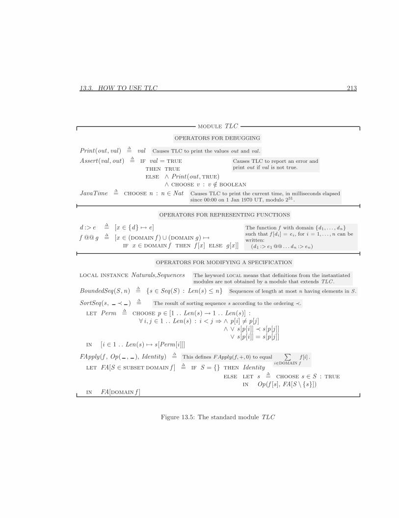
13.3. HOW TO USE TLC 213
module TLC
OPERATORS FOR DEBUGGING
Print(out , val) ∆= val Causes TLC to print the values out and val .
Assert(val , out) ∆= if val = truethen trueelse ∧ Print(out ,true)
∧ choose v : v /∈ boolean
Causes TLC to report an error andprint out if val is not true.
JavaTime ∆= choose n : n ∈ Nat Causes TLC to print the current time, in milliseconds elapsedsince 00:00 on 1 Jan 1970 UT, modulo 231.
OPERATORS FOR REPRESENTING FUNCTIONS
d :> e ∆= [x ∈ {d} 7→ e]
f @@ g ∆= [x ∈ (domain f ) ∪ (domain g) 7→if x ∈ domain f then f [x ] else g[x ]]
The function f with domain {d1, . . . , dn}such that f [d i ] = ei , for i = 1, . . . ,n can bewritten:
(d1 :> e1 @@ . . . dn :> en)
OPERATORS FOR MODIFYING A SPECIFICATION
local instance Naturals,Sequences The keyword local means that definitions from the instantiatedmodules are not obtained by a module that extends TLC .
BoundedSeq(S ,n) ∆= {s ∈ Seq(S ) : Len(s) ≤ n} Sequences of length at most n having elements in S .
SortSeq(s , ≺ ) ∆= The result of sorting sequence s according to the ordering ≺.
let Perm ∆= choose p ∈ [1 . . Len(s)→ 1 . . Len(s)] :∀ i , j ∈ 1 . . Len(s) : i < j ⇒ ∧ p[i ] 6= p[j ]
∧ ∨ s [p[i ]] ≺ s [p[j ]]∨ s [p[i ]] = s [p[j ]]
in [i ∈ 1 . . Len(s) 7→ s [Perm[i ]]]
FApply(f , Op( , ), Identity) ∆= This defines FApply(f,+, 0) to equal∑
i∈domain f
f [i] .
let FA[S ∈ subset domain f ] ∆= if S = {} then Identityelse let s ∆= choose s ∈ S : true
in Op(f [s ], FA[S \ {s}])in FA[domain f ]
Figure 13.5: The standard module TLC
214 CHAPTER 13. THE TLC MODEL CHECKER
the definition in the module, since it would first have to evaluate the infinite setSeq(S ). TLC could evaluate it from the equivalent definition
BoundedSeq(S ,n) ∆= union {[1 . . m → S ] : m ∈ 0 . . n}but evaluation is faster with the overriding Java implementation.
The TLC module next defines the operator SortSeq. If s is a finite sequenceand ≺ is a total ordering relation on its elements, then SortSeq(s ,≺) is thesequence obtained from s by sorting its elements according to ≺. For example,SortSeq(〈3, 1, 3, 8〉, >) equals 〈8, 3, 3, 1〉. The Java implementation of SortSeqallows TLC to evaluate it more efficiently than a user-defined sorting operator.For example, because the following definition of the operator FastSort , whichmakes use of SortSeq to do the actual sorting, TLC can evaluate it faster thanthe definition given above on page 202.
FastSort(S ) ∆=let MakeSeq[SS ∈ BoundedSubSet(S ,Cardinality(S ))] ∆=
if SS = then 〈 〉else let ss ∆= choose ss ∈ SS : true
in Append(MakeSeq[SS {ss}], ss)in SortSeq(MakeSeq[S ], <)
The TLC module ends by defining the operator FApply. If f is a func-tion with finite domain, and Op is an operator that takes two arguments, thenFApply(f ,Op, Id) equals
Op(f [d1], Op(f [d2], Op( . . . Op(f [dn ], Id) . . .)
where d1, . . . , dn are the elements in the domain of f , listed in some arbitraryorder. Using FApply to avoid a recursive definition can speed up TLC. Forexample, the factorial function fact can be defined by
fact(n) ∆= FApply([i ∈ 1 . . n 7→ i ], ∗, 1)
TLC can compute factorials from this definition faster than from the standardrecursive definition on page 54.
13.3.4 Checking Action Invariance
Section 5.7 on page 60 discusses two different kinds of invariants. A state pred-icate Inv that satisfies Spec ⇒ 2Inv is called an invariant of the specificationSpec. This is the kind of invariance property that TLC checks. If Inv satis- When v is the tu-
ple of all relevantvariables, Inv isan invariant of[Next ]v iff it is aninvariant of Next .
fies Inv ∧ [Next ]v ⇒ Inv ′, then Inv is called an invariant of the action [Next ]v .It’s not hard to see that Inv is an invariant of action [Next ]v iff it satisfiesInv ∧ 2[Next ]v ⇒ 2Inv . We can therefore check if Inv is an invariant of an
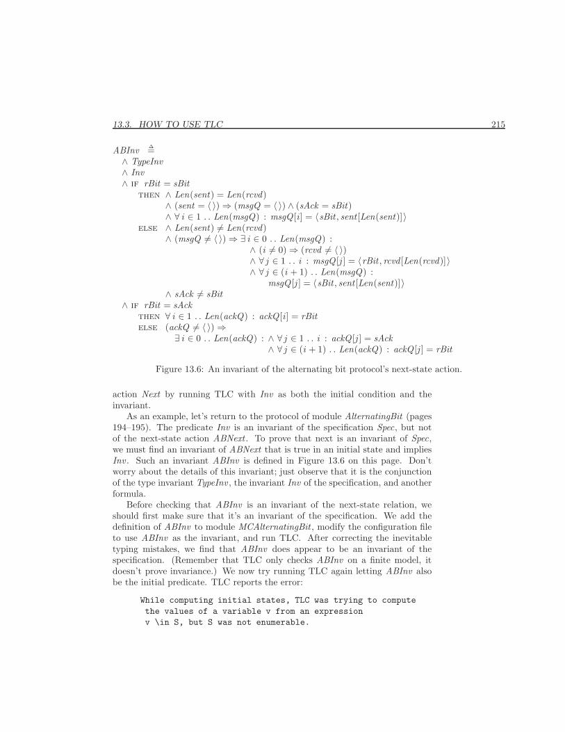
13.3. HOW TO USE TLC 215
ABInv ∆=∧ TypeInv∧ Inv∧ if rBit = sBit
then ∧ Len(sent) = Len(rcvd)∧ (sent = 〈 〉)⇒ (msgQ = 〈 〉) ∧ (sAck = sBit)∧ ∀ i ∈ 1 . . Len(msgQ) : msgQ [i ] = 〈sBit , sent [Len(sent)]〉
else ∧ Len(sent) 6= Len(rcvd)∧ (msgQ 6= 〈 〉)⇒ ∃ i ∈ 0 . . Len(msgQ) :
∧ (i 6= 0)⇒ (rcvd 6= 〈 〉)∧ ∀ j ∈ 1 . . i : msgQ [j ] = 〈rBit , rcvd [Len(rcvd)]〉∧ ∀ j ∈ (i + 1) . . Len(msgQ) :
msgQ [j ] = 〈sBit , sent [Len(sent)]〉∧ sAck 6= sBit
∧ if rBit = sAckthen ∀ i ∈ 1 . . Len(ackQ) : ackQ [i ] = rBitelse (ackQ 6= 〈 〉)⇒
∃ i ∈ 0 . . Len(ackQ) : ∧ ∀ j ∈ 1 . . i : ackQ [j ] = sAck∧ ∀ j ∈ (i + 1) . . Len(ackQ) : ackQ [j ] = rBit
Figure 13.6: An invariant of the alternating bit protocol’s next-state action.
action Next by running TLC with Inv as both the initial condition and theinvariant.
As an example, let’s return to the protocol of module AlternatingBit (pages194–195). The predicate Inv is an invariant of the specification Spec, but notof the next-state action ABNext . To prove that next is an invariant of Spec,we must find an invariant of ABNext that is true in an initial state and impliesInv . Such an invariant ABInv is defined in Figure 13.6 on this page. Don’tworry about the details of this invariant; just observe that it is the conjunctionof the type invariant TypeInv , the invariant Inv of the specification, and anotherformula.
Before checking that ABInv is an invariant of the next-state relation, weshould first make sure that it’s an invariant of the specification. We add thedefinition of ABInv to module MCAlternatingBit , modify the configuration fileto use ABInv as the invariant, and run TLC. After correcting the inevitabletyping mistakes, we find that ABInv does appear to be an invariant of thespecification. (Remember that TLC only checks ABInv on a finite model, itdoesn’t prove invariance.) We now try running TLC again letting ABInv alsobe the initial predicate. TLC reports the error:
While computing initial states, TLC was trying to computethe values of a variable v from an expressionv \in S, but S was not enumerable.
216 CHAPTER 13. THE TLC MODEL CHECKER
at line 20, column 15 to line 20, column 41 in: AlternatingBit
Recall that TLC computes the initial states by computing the conjuncts of theinitial predicate in order. (See Section 13.2.5 on page 203). From the definitionof TypeInv , we see that it first tries to compute the possible values of msgQ byevaluating
msgQ ∈ Seq({0, 1} ×Data)
Since Seq({0, 1} × Data) is an infinite set, containing sequences of any length,this yields an infinite number of possible values of msgQ , so TLC gives up. (Re-member that TLC first computes all states satisfying the initial condition, then itthrows away those that don’t satisfy the constraint.) So, we must modify ABInvto specify only a finite set of initial values. We add to the MCAlternatingBitmodule a predicate BTypeInv that is a bounded version of TypeInv . For exam-ple, it specifies the initial value of msgQ by
msgQ ∈ BoundedSeq({0, 1} ×Data, msgQLen)
where the operator BoundedSeq, defined in the TLC module, is explained onpages 212–214, and msgQLen is the parameter of MCAlternatingBit used in theconstraint to bound the length of msgQ . We then define BdedABInv to be thesame as ABInv , except with TypeInv replaced by BTypeInv , and run TLC withBdedABInv as the initial condition and ABInv as the invariant, using the sameconstraint as before. (Do you see why we can’t use BdedABInv as the invariant?If not, review Section 13.2.6.)
When computing the initial states, TLC examines every state satisfyingBTypeInv , throwing away those that don’t satisfy the rest of BdedABInv . SinceBoundedSeq(S ,n) has more than Cardinality(S )n elements, the number of initialstates that TLC examines is greater than
8 ∗ 2msgQLen+ackQLen ∗DmsgQLen+2∗sentLen
where D is the cardinality of Data. (I am taking sentLen to be the bound on thelength of the queues sent and rcvd .) This number grows much faster than thenumber of reachable states, estimated by formula (13.2) on page 198. Typically,TLC can check an invariant of an action only on a very small model—muchsmaller than the models on which it can check an invariant of a specification.
We can use BdedABInv as the initial predicate only because its first conjunctis the type invariant BTypeInv . If we interchange its first two conjuncts, thenTLC will try to evaluate Inv before evaluating BTypeInv . Evaluating the firstconjunct
Len(rcvd) ∈ {Len(sent)− 1,Len(sent)}of Inv causes TLC to produce the error message
13.3. HOW TO USE TLC 217
The identifier rcvd is not assigned a value in thecurrent context . . .
When using TLC to check that a predicate P is an invariant of an action,evaluating P must specify the value of each variable v with a conjunct of theform v ∈ S before that value is used.
13.3.5 Checking Implementation
In industrial applications, a TLA+ specification is likely to be the only formaldescription of a system. Such a specification is correct if it means what weintended, which is not a formalizable concept. By formalizing some of our in-tentions as invariants, we can use TLC to help catch errors in the specification.Sometimes, a specification SL is a lower-level view of a system for which wehave a higher-level specification SH . We usually regard SH as the system’sspecification and SL as an implementation, and take correctness of SL to meanthat it implies SH . This situation occurred in Chapter 5, with the implemen-tation SL being the specification of the write-through cache (formula Spec ofmodule WriteThroughCache) and the specification SH being the specificationof a linearizable memory (formula Spec of the Memory module).
We saw in Section 5.8 that this requires proving a formula of the form:
Init ∧ 2[Next ]v ⇒ HInit ∧ 2[HNext ]hv(13.4)
This formula is true iff the following two conditions hold:
1. Init implies HInit
2. In every behavior satisfying Init ∧2[Next ]v , every step is an [HNext ]hvstep.
TLC allows you to check these conditions as follows. First, specify as usual inthe configuration file that Init and Next are the initial predicate and next-stateaction. To check condition 1, specify HInit as the implied-init predicate byadding the following to the configuration file:4
IMPLIED-INIT HInit
TLC will report an error if it finds an initial state (one satisfying Init) that doesnot satisfy HInit . To check condition 2, first define a new symbol, say SqHNext ,in the TLA module:
SqHNext ∆= [HNext ]hv
Then, specify SqHNext as the implied-action formula by adding the followingto the configuration file:
4TLC does not yet support the implied−init field. Until it does, you can have it checkcondition 1 by running it with the initial predicate Init ∧ Assert(HInit , “HInit false”).
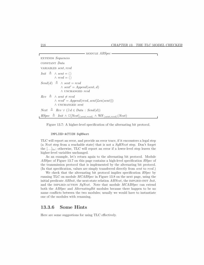
218 CHAPTER 13. THE TLC MODEL CHECKER
module ABSpecextends Sequencesconstant Datavariables sent , rcvd
Init ∆= ∧ sent = 〈 〉∧ rcvd = 〈 〉
Send(d) ∆= ∧ sent = rcvd∧ sent ′ = Append(sent , d)∧ unchanged rcvd
Rcv ∆= ∧ sent 6= rcvd∧ rcvd ′ = Append(rcvd , sent [Len(sent)])∧ unchanged sent
Next ∆= Rcv ∨ (∃ d ∈ Data : Send(d))
HSpec ∆= Init ∧ 2[Next ]〈sent,rcvd 〉 ∧ WF〈sent,rcvd 〉(Next)
Figure 13.7: A higher-level specification of the alternating bit protocol.
IMPLIED-ACTION SqHNext
TLC will report an error, and provide an error trace, if it encounters a legal step(a Next step from a reachable state) that is not a SqHNext step. Don’t forgetthe [. . .]hv ; otherwise, TLC will report an error if a lower-level step leaves thehigher-level variables unchanged.
As an example, let’s return again to the alternating bit protocol. ModuleABSpec of Figure 13.7 on this page contains a high-level specification HSpec ofthe transmission protocol that is implemented by the alternating bit protocol.(In that specification, values are simply transferred directly from sent to rcvd .)
We check that the alternating bit protocol implies specification HSpec byrunning TLC on module MCABSpec in Figure 13.8 on the next page, using theinitial predicate ABInit , the next-state relation ABNext , the implied-init Init ,and the implied-action SqNext . Note that module MCABSpec can extendboth the ABSpec and AlternatingBit modules because there happen to be noname conflicts between the two modules; usually we would have to instantiateone of the modules with renaming.
13.3.6 Some Hints
Here are some suggestions for using TLC effectively.
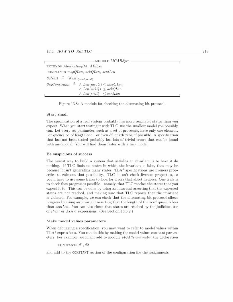
13.3. HOW TO USE TLC 219
module MCABSpecextends AlternatingBit , ABSpecconstants msgQLen, ackQLen, sentLen
SqNext ∆= [Next ]〈sent,rcvd 〉SeqConstraint ∆= ∧ Len(msgQ) ≤ msgQLen
∧ Len(ackQ) ≤ ackQLen∧ Len(sent) ≤ sentLen
Figure 13.8: A module for checking the alternating bit protocol.
Start small
The specification of a real system probably has more reachable states than youexpect. When you start testing it with TLC, use the smallest model you possiblycan. Let every set parameter, such as a set of processes, have only one element.Let queues be of length one—or even of length zero, if possible. A specificationthat has not been tested probably has lots of trivial errors that can be foundwith any model. You will find them faster with a tiny model.
Be suspicious of success
The easiest way to build a system that satisfies an invariant is to have it donothing. If TLC finds no states in which the invariant is false, that may bebecause it isn’t generating many states. TLA+ specifications use liveness prop-erties to rule out that possibility. TLC doesn’t check liveness properties, soyou’ll have to use some tricks to look for errors that affect liveness. One trick isto check that progress is possible—namely, that TLC reaches the states that youexpect it to. This can be done by using an invariant asserting that the expectedstates are not reached, and making sure that TLC reports that the invariantis violated. For example, we can check that the alternating bit protocol allowsprogress by using an invariant asserting that the length of the rcvd queue is lessthan sentLen. You can also check that states are reached by the judicious useof Print or Assert expressions. (See Section 13.3.2.)
Make model values parameters
When debugging a specification, you may want to refer to model values withinTLA+ expressions. You can do this by making the model values constant param-eters. For example, we might add to module MCAlternatingBit the declaration
constants d1, d2
and add to the CONSTANT section of the configuration file the assignments
220 CHAPTER 13. THE TLC MODEL CHECKER
d1 = d1 d2 = d2
which assign to the constant parameters d1 and d2 the model values d1 and d2,respectively.
Don’t start over after every error
After you’ve eliminated the errors that are easy to find, TLC may have to run fora long time before finding an error. It often takes more than one try to correctlycorrect an error, and it can be frustrating to run TLC for an hour only to findthat you made a silly mistake in the correction. If the error was discovered whentaking a step from a correct state, then it’s a good idea to check your correctionby starting TLC from that state. You can do this by using the state printed byTLC to define the initial predicate to be used by TLC.
Another way to avoid starting from scratch after an error is by using check-points. A checkpoint saves the set of reached states and the queue of unexploredstates.5 It does not save any other information about the specification. You canrestart a specification from a checkpoint even if you have changed the specifica-tion, as long as the specification’s variables and the values that they can assumehaven’t changed. If TLC finds an error after running for a long time, you maywant to continue it from the last checkpoint instead of having it recheck all thestates it had already checked.
Check everything you can
A single invariant seldom expresses correctness of a specification. Write and letTLC check as many different invariance properties as you can. If you think thatsome predicate should be an invariant, let TLC test if it is. Discovering that thepredicate is not an invariant may not signal an error, in the specification, but itwill probably teach you something about your specification.
Try to check liveness
Although TLC can’t directly check liveness properties, you can sometimes checkthem indirectly by modifying the specification. A liveness property asserts thatsomething must eventually happen. Sometimes, you can check such a propertyby checking that the property must hold after the system has taken a certainnumber of steps. For example, suppose you want to check that the specification
Spec ∆= Init ∧ 2[Next ]v ∧WFv (Next)
satisfies the property P ; Q for some predicates P and Q . In most cases, Spec The operator; (leads-to)is explained onpage 90.
implies P ; Q iff it implies that, whenever P is true, Q must become true5Some of the reached states may not be saved, so TLC may explore again some states that
had been reached before the checkpoint.
13.4. WHAT TLC DOESN’T DO 221
within N steps, where N is some function of the constant parameters. You cancheck this by adding a variable ctr that counts the number of steps taken sinceP became true, and is reset when Q becomes true. You can check that P alwaysleads to Q within N steps by checking that ctr is never greater than N . Moreprecisely, you can define a new specification whose initial predicate is
Init ∧ (ctr = if P ∧ ¬Q then 0 else − 1)
and next-state action is
∧ Next∧ ctr ′ = if ¬Q ′ ∧ (ctr ≥ 0 ∨ P ′) then ctr + 1 else − 1
You can then use TLC to check that ctr ≤ N is an invariant of this specification.
Use symmetry to save time
For many specifications, TLC will take a long time to check all the reachablestates for a nontrivial model. One way to have it use less time is to reduce thenumber of reachable states it must check. There is often some symmetry in thespecification that makes certain states equivalent in terms of finding errors. Twostates s and t are equivalent if a behavior starting from state s can produce anerror iff one starting from state t can. If s and t are equivalent, there is no needto explore states reachable from both of them. For example, the alternating bitprotocol does not depend on the actual values being sent. So, permuting all thedata values in any state produces an equivalent state.
The constraint can often be used to keep TLC from exploring the successorsof different equivalent states. For example, we can exploit the symmetry of thealternating bit protocol under permutation of data values as follows. We usea model in which Data is a set of numbers and conjoin to the constraint therequirement that the elements of sent are sorted:
∀ i , j ∈ 1 . . Len(sent) : (i � j )⇒ (sent [i ] � sent [j ])
For the model size specified by the configuration file of Figure 13.4, this extraconstraint reduces the number of reachable states from 2312 to 1482. When thenumber of elements in Data is increased to 3 and sentLen is increased to 4, itreduces the number of reachable states from 22058 to 6234.
13.4 What TLC Doesn’t Do
We would like TLC to generate all the behaviors that satisfy a specification. Butno program can do this for an arbitrary specification. I have already mentionedvarious limitations of TLC. There are some other limitations that you may
222 CHAPTER 13. THE TLC MODEL CHECKER
stumble on. One of them is that the Java classes that override the Naturals andIntegers modules will handle only numbers in the interval −231 . . (231 − 1).
An easier goal would be for every behavior that TLC does generate to sat-isfy the (safety part) of the specification. However, for reasons of efficiency,TLC doesn’t always meet this goal. In particular, it doesn’t preserve the pre-cise semantics of choose . As explained in Section 15.1, if S equals T , thenchoose x ∈ S : P should equal choose x ∈ T : P . However, if the expressionsdon’t have a uniquely-defined value, then TLC guarantees this only if S and Tare syntactically the same. For example, TLC might compute different valuesfor the two expressions
choose x ∈ {1, 2, 3} : x < 3 choose x ∈ {3, 2, 1} : x < 3
A similar violation of the semantics of TLA+exists with case expressions, whosesemantics are defined (in Section 15.1.4) in terms of choose.
TLC Version 1 the following additional limitations, most of which should befixed in version 2. Telling us which ones you find to be a nuisance will helpensure that they really are fixed in Version 2.
• TLC doesn’t handle specifications that use the instance statement.
• TLC doesn’t properly handle Cartesian products of more than two sets.Thus, instead of writing S × T ×U , you have to write
{〈s , t , u 〉 : s ∈ S , t ∈ T , u ∈ U }• You cannot put infix, prefix, or postfix operators in the CONSTANT section
of the configuration file. Hence, neither of the following replacements mayappear in the configuration file:
++ <- Foo Bar <- &
• You cannot use an infix, prefix, or postfix operator as the argument ofa higher-order operator. For example, if IsPartialOrder is the operatordescribed on pages 70–71, you cannot write IsPartialOrder(<, Nat). Toget around this problem, you can define
LessThan(a, b) ∆= a < b
and then write IsPartialOrder(LessThan, Nat).
• You cannot define an infix, prefix, or postfix operator in a let expression.
• The Java class that overrides the Sequences module does not properlyhandle the BoundedSeq operator. You can define a replacement operatorfor it, using the definition on pages 212–214, that works properly.
• The Java class that overrides the standard Bags module does not imple-ment the SubBag operator.
13.5. FUTURE PLANS 223
• TLC does not check that a symbol is defined before it is used. This meansthat TLC will accept illegal recursive operator definitions like
Silly(foo) ∆= Silly(foo + 1)
• The Java classes that override the Naturals and Integers modules produceincorrect results, rather than an error message, if a computation yields anumber outside the interval −231 . . (231 − 1).
• TLC doesn’t implement the · (action composition) operator.
• TLC treats strings as primitive values, and not as functions. It thus con-siders the legal TLA+ expression “abc”[2] to be an error. It also handlesonly strings containing letters, numbers, spaces, and the following ASCIIcharacters:
< > ? , . / : ; [ ] { } | ~ ! @ # $ % ^ & * ( ) _ - + =
• TLC allows constants to be replaced by nonconstants operators. Doing Replacement isexplained in Sec-tion 13.2.3.
so may cause TLC to produce incorrect results. (Version 1 also allowsnonconstants to be replaced; this might not be allowed in Version 2.)
13.5 Future Plans
The following additions and improvements to future versions of TLC are beingconsidered. It is unlikely that they will all be implemented; recommendationsof which ones are most important would be useful.
• Check liveness properties.
• Handle the type of compositional specifications, described in Section 10.2,that have conjuncts of the form 2IsFcnOn(f , S ), and the next-state actionspecifies only the values of f [s ] for s ∈ S .
• Have the progress reports contain separate counts of generated states thatdo and don’t satisfy the constraint.
• Introduce subclasses of model values, where a model value is comparableonly with model values in its own subclass. This requires also adding someway of handling the construct choose x : x /∈ S .
• Improve debugging information as follows:
– Print out the context at the point of the error—including variablevalues, and the values of bound variables.
– Identify the disjunct of the next-state action responsible for each stepwhen printing a behavior.
224 CHAPTER 13. THE TLC MODEL CHECKER
– More precisely identify the place within the specification where anerror occurs.
– When an invariant is found to be false, have TLC print out why it isfalse—that is, which conjunct or conjuncts are false.
• Add a debugging mode in which TLC won’t stop for an error, but will justkeep going.
• Add some coverage analysis, indicating which parts of the next-state rela-tion never evaluated to true.
• Add some support for using symmetry to reduce the state space searched.
• Have TLC check all assumptions.
13.6 The Fine Print: What TLC Really Does
We now describe in more detail what TLC does. This section is for the intel-lectually curious and mathematically sophisticated. Most users will not want toread it.
This section specifies the results produced by TLC, not the actual algorithmsit uses to compute those results. Moreover, it specifies only what TLC guaran-tees to do. TLC may actually do better, producing a correct result when thespecification allows it to report an error.
13.6.1 TLC Values
Section 13.2.1 (page 198) describes TLC values. That description was incompletein two ways. First, it did not precisely define when values are comparable. Theprecise definition is that two TLC values are comparable iff the following rulesimply that they are:
1. Two primitive values are comparable if they have the same value type.
This rule implies that “abc” and “123” are comparable. But “abc” and123 are not comparable.
2. A model value is comparable with any value. (It is equal only to itself.)
3. Two sets are comparable if they have different numbers of elements, or ifthey have the same numbers of elements and all the elements in one setare comparable with all the elements in the other.
This rule implies that {1} and {“a”, “b”} are comparable and that {1, 2}and {2, 3} are comparable. However, {1, 2} and {“a”, “b”} are not com-parable.
13.6. THE FINE PRINT: WHAT TLC REALLY DOES 225
4. Two functions f and g are comparable if (i) their domains are comparableand (ii) if their domains are equal, then f [x ] and g[x ] are comparable forevery element x in their domains.
This rule implies that 〈1, 2〉 and 〈“a”, “b”, “c”〉 are comparable, and that〈1, “a”〉 and 〈2, “bc”〉 are comparable. However, 〈1, 2〉 and 〈“a”, “b”〉 arenot comparable.
Section 13.2.1 also failed to mention that additional primitive value types can TLC Version 1does not supportthe introductionof new primitivevalue types.
be introduced by Java classes that override modules. The primitive TLC valuetypes are thus Booleans, integers, strings, model values, and any additional valuetypes introduced by overriding.
13.6.2 Overridden Values
As explained in Section 13.2.4 above, an extended module may be overridden bya Java class. All the values and operators defined by the module are replaced byspecial overridden values. For example, the Java class that overrides the Naturalsmodule replaces Nat and + by overridden values. An overridden module maynot have parameters.
13.6.3 Expression Evaluation
TLC evaluates expressions when performing three different tasks:
• It evaluates the initial predicate to compute the set of initial states.
• It evaluates the next-state action to compute the set of states reachablefrom a given state by a step of that action.
• It evaluates an invariant when checking that a reachable state is correct.
The result of successfully evaluating an expression is a TLC value. Evaluationmay fail, in which case TLC reports an error and halts.
TLC evaluates an expression in a context, which is an assignment of meaningsto user-defined symbols, parameters, variables, and primed variables. A meaningis a TLA+ expression formed from the built-in operators of TLA+, TLC values,and overridden values. Variables and primed variables can be assigned onlyTLC values. For example, consider a module that has two variables x and y.To compute the next states starting in a state with x = 2 and y = {“a”}, TLCevaluates the next-state relation in the context C in which the defined symbolshave the meanings assigned to them by the module, the module’s parametershave the values assigned to them by the configuration file, x is assigned the value2, y is assigned the value {“a”}, and x ′ and y ′ have no meanings assigned tothem. Suppose the next-state action has the form (x ′ = e) ∧A. TLC computes
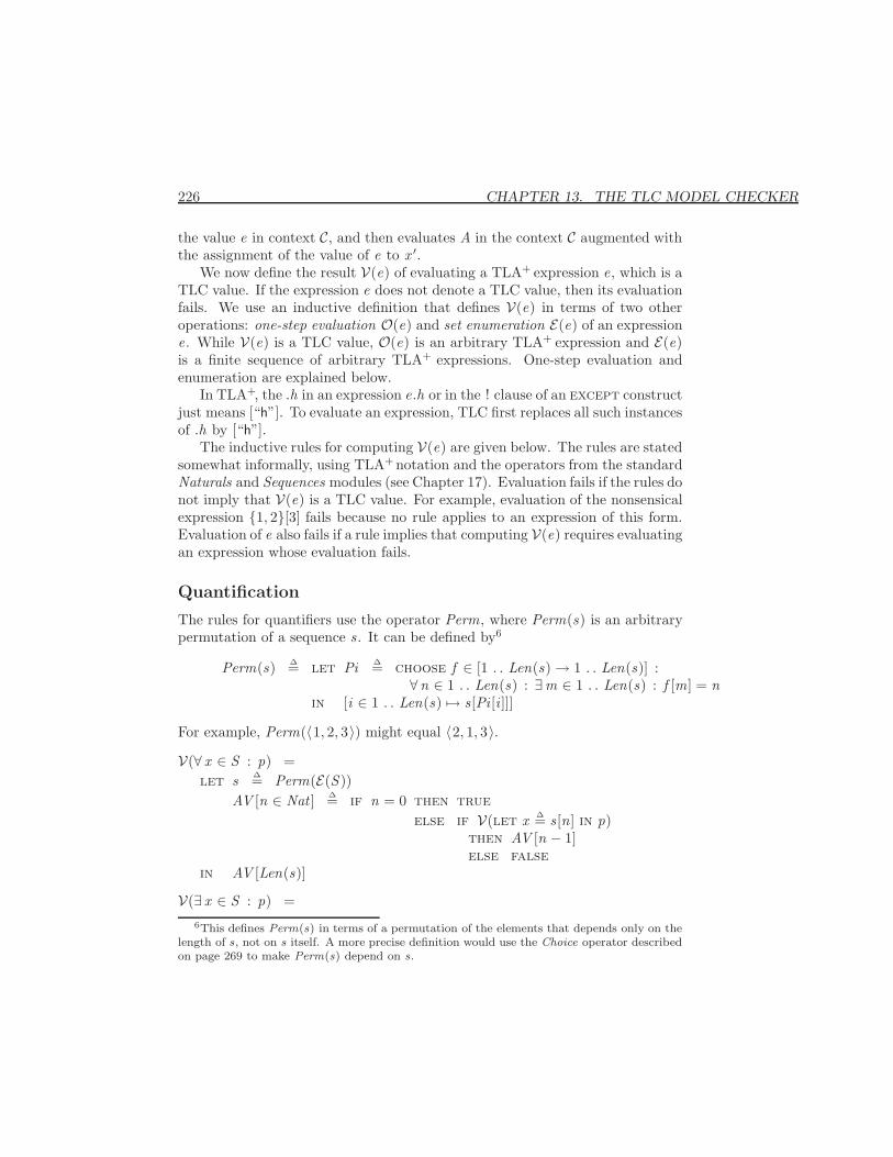
226 CHAPTER 13. THE TLC MODEL CHECKER
the value e in context C, and then evaluates A in the context C augmented withthe assignment of the value of e to x ′.
We now define the result V(e) of evaluating a TLA+ expression e, which is aTLC value. If the expression e does not denote a TLC value, then its evaluationfails. We use an inductive definition that defines V(e) in terms of two otheroperations: one-step evaluation O(e) and set enumeration E(e) of an expressione. While V(e) is a TLC value, O(e) is an arbitrary TLA+ expression and E(e)is a finite sequence of arbitrary TLA+ expressions. One-step evaluation andenumeration are explained below.
In TLA+, the .h in an expression e.h or in the ! clause of an except constructjust means [“h”]. To evaluate an expression, TLC first replaces all such instancesof .h by [“h”].
The inductive rules for computing V(e) are given below. The rules are statedsomewhat informally, using TLA+ notation and the operators from the standardNaturals and Sequences modules (see Chapter 17). Evaluation fails if the rules donot imply that V(e) is a TLC value. For example, evaluation of the nonsensicalexpression {1, 2}[3] fails because no rule applies to an expression of this form.Evaluation of e also fails if a rule implies that computing V(e) requires evaluatingan expression whose evaluation fails.
Quantification
The rules for quantifiers use the operator Perm, where Perm(s) is an arbitrarypermutation of a sequence s . It can be defined by6
Perm(s) ∆= let Pi ∆= choose f ∈ [1 . . Len(s)→ 1 . . Len(s)] :∀n ∈ 1 . . Len(s) : ∃m ∈ 1 . . Len(s) : f [m] = n
in [i ∈ 1 . . Len(s) 7→ s [Pi [i ]]]
For example, Perm(〈1, 2, 3〉) might equal 〈2, 1, 3〉.V(∀ x ∈ S : p) =
let s ∆= Perm(E(S ))AV [n ∈ Nat ] ∆= if n = 0 then true
else if V(let x ∆= s [n] in p)then AV [n − 1]else false
in AV [Len(s)]
V(∃ x ∈ S : p) =
6This defines Perm(s) in terms of a permutation of the elements that depends only on thelength of s, not on s itself. A more precise definition would use the Choice operator describedon page 269 to make Perm(s) depend on s.
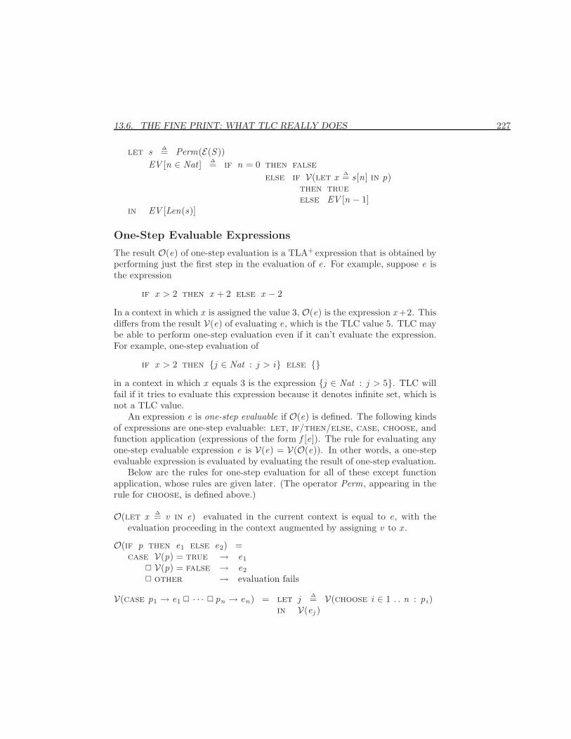
13.6. THE FINE PRINT: WHAT TLC REALLY DOES 227
let s ∆= Perm(E(S ))EV [n ∈ Nat ] ∆= if n = 0 then false
else if V(let x ∆= s [n] in p)then trueelse EV [n − 1]
in EV [Len(s)]
One-Step Evaluable Expressions
The result O(e) of one-step evaluation is a TLA+ expression that is obtained byperforming just the first step in the evaluation of e. For example, suppose e isthe expression
if x > 2 then x + 2 else x − 2
In a context in which x is assigned the value 3, O(e) is the expression x +2. Thisdiffers from the result V(e) of evaluating e, which is the TLC value 5. TLC maybe able to perform one-step evaluation even if it can’t evaluate the expression.For example, one-step evaluation of
if x > 2 then {j ∈ Nat : j > i} else {}in a context in which x equals 3 is the expression {j ∈ Nat : j > 5}. TLC willfail if it tries to evaluate this expression because it denotes infinite set, which isnot a TLC value.
An expression e is one-step evaluable if O(e) is defined. The following kindsof expressions are one-step evaluable: let, if/then/else, case, choose, andfunction application (expressions of the form f [e]). The rule for evaluating anyone-step evaluable expression e is V(e) = V(O(e)). In other words, a one-stepevaluable expression is evaluated by evaluating the result of one-step evaluation.
Below are the rules for one-step evaluation for all of these except functionapplication, whose rules are given later. (The operator Perm, appearing in therule for choose, is defined above.)
O(let x ∆= v in e) evaluated in the current context is equal to e, with theevaluation proceeding in the context augmented by assigning v to x .
O(if p then e1 else e2) =case V(p) = true → e1
2 V(p) = false → e2
2 other → evaluation fails
V(case p1 → e1 2 · · · 2 pn → en) = let j ∆= V(choose i ∈ 1 . . n : pi)in V(ej )
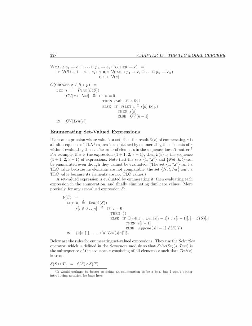
228 CHAPTER 13. THE TLC MODEL CHECKER
V(case p1 → e1 2 · · · 2 pn → en 2other→ e) =if V(∃ i ∈ 1 . . n : pi) then V(case p1 → e1 2 · · · 2 pn → en)
else V(e)
O(choose x ∈ S : p) =let s ∆= Perm(E(S ))
CV [n ∈ Nat ] ∆= if n = 0then evaluation failselse if V(let x ∆= s [n] in p)
then s [n]else CV [n − 1]
in CV [Len(s)]
Enumerating Set-Valued Expressions
If e is an expression whose value is a set, then the result E(e) of enumerating e isa finite sequence of TLA+ expressions obtained by enumerating the elements of ewithout evaluating them. The order of elements in the sequence doesn’t matter.7
For example, if e is the expression {1 + 1, 2, 3 − 1}, then E(e) is the sequence〈1 + 1, 2, 3 − 1〉 of expressions. Note that the sets {1, “a”} and {Nat , Int} canbe enumerated even though they cannot be evaluated. (The set {1, “a”} isn’t aTLC value because its elements are not comparable; the set {Nat , Int} isn’t aTLC value because its elements are not TLC values.)
A set-valued expression is evaluated by enumerating it, then evaluating eachexpression in the enumeration, and finally eliminating duplicate values. Moreprecisely, for any set-valued expression S :
V(S ) =let n ∆= Len(E(S ))
s [i ∈ 0 . . n] ∆= if i = 0then 〈 〉else if ∃ j ∈ 1 . . Len(s [i − 1]) : s [i − 1][j ] = E(S )[i ]
then s [i − 1]else Append(s [i − 1], E(S )[i ])
in {s [n][1], . . . , s [n][Len(s [n])]}Below are the rules for enumerating set-valued expressions. They use the SelectSeqoperator, which is defined in the Sequences module so that SelectSeq(s ,Test) isthe subsequence of the sequence s consisting of all elements e such that Test(e)is true.
E(S ∪ T ) = E(S ) ◦ E(T )
7It would perhaps be better to define an enumeration to be a bag, but I won’t botherintroducing notation for bags here.
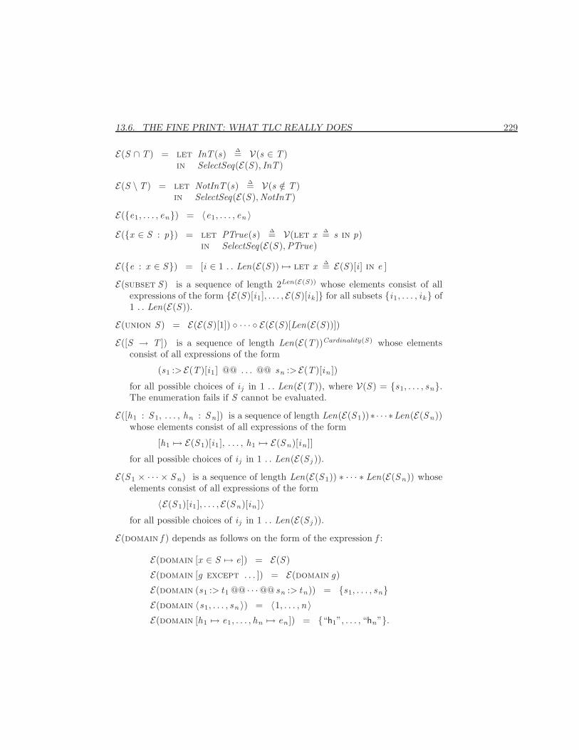
13.6. THE FINE PRINT: WHAT TLC REALLY DOES 229
E(S ∩ T ) = let InT (s) ∆= V(s ∈ T )in SelectSeq(E(S ), InT )
E(S \T ) = let NotInT (s) ∆= V(s /∈ T )in SelectSeq(E(S ),NotInT )
E({e1, . . . , en}) = 〈e1, . . . , en 〉E({x ∈ S : p}) = let PTrue(s) ∆= V(let x ∆= s in p)
in SelectSeq(E(S ),PTrue)
E({e : x ∈ S}) = [i ∈ 1 . . Len(E(S )) 7→ let x ∆= E(S )[i ] in e ]
E(subset S ) is a sequence of length 2Len(E(S)) whose elements consist of allexpressions of the form {E(S )[i1], . . . , E(S )[ik ]} for all subsets {i1, . . . , ik} of1 . . Len(E(S )).
E(union S ) = E(E(S )[1]) ◦ · · · ◦ E(E(S )[Len(E(S ))])
E([S → T ]) is a sequence of length Len(E(T ))Cardinality(S) whose elementsconsist of all expressions of the form
(s1 :> E(T )[i1 ] @@ . . . @@ sn :> E(T )[in ])
for all possible choices of i j in 1 . . Len(E(T )), where V(S ) = {s1, . . . , sn}.The enumeration fails if S cannot be evaluated.
E([h1 : S 1, . . . , hn : Sn ]) is a sequence of length Len(E(S 1))∗ · · · ∗Len(E(Sn))whose elements consist of all expressions of the form
[h1 7→ E(S 1)[i1], . . . , h1 7→ E(Sn)[in ]]
for all possible choices of i j in 1 . . Len(E(S j )).
E(S 1 × · · · × Sn) is a sequence of length Len(E(S 1)) ∗ · · · ∗ Len(E(Sn)) whoseelements consist of all expressions of the form
〈E(S 1)[i1], . . . , E(Sn)[in ]〉for all possible choices of i j in 1 . . Len(E(S j )).
E(domain f ) depends as follows on the form of the expression f :
E(domain [x ∈ S 7→ e]) = E(S )
E(domain [g except . . . ]) = E(domain g)
E(domain (s1 :> t1 @@ · · ·@@ sn :> tn)) = {s1, . . . , sn}E(domain 〈s1, . . . , sn 〉) = 〈1, . . . ,n 〉E(domain [h1 7→ e1, . . . , hn 7→ en ]) = {“h1”, . . . , “hn”}.
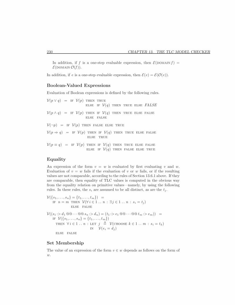
230 CHAPTER 13. THE TLC MODEL CHECKER
In addition, if f is a one-step evaluable expression, then E(domain f ) =E(domainO(f )).
In addition, if e is a one-step evaluable expression, then E(e) = E(O(e)).
Boolean-Valued Expressions
Evaluation of Boolean expressions is defined by the following rules.
V(p ∨ q) = if V(p) then trueelse if V(q) then true else FALSE
V(p ∧ q) = if V(p) then if V(q) then true else falseelse false
V(¬p) = if V(p) then false else true
V(p ⇒ q) = if V(p) then if V(q) then true else falseelse true
V(p ≡ q) = if V(p) then if V(q) then true else falseelse if V(q) then false else true
Equality
An expression of the form v = w is evaluated by first evaluating v and w .Evaluation of v = w fails if the evaluation of v or w fails, or if the resultingvalues are not comparable, according to the rules of Section 13.6.1 above. If theyare comparable, then equality of TLC values is computed in the obvious wayfrom the equality relation on primitive values—namely, by using the followingrules. In these rules, the s i are assumed to be all distinct, as are the t j .
V({s1, . . . , sn} = {t1, . . . , tm}) =if n = m then V(∀ i ∈ 1 . . n : ∃ j ∈ 1 . . n : s i = t j )
else false
V((s1 :> d1 @@ · · ·@@ sn :> dn) = (t1 :> e1 @@ · · ·@@ tm :> em)) =if V({s1, . . . , sn} = {t1, . . . , tm})
then ∀ i ∈ 1 . . n : let j ∆= V(choose k ∈ 1 . . m : s i = tk )in V(ei = d j )
else false
Set Membership
The value of an expression of the form v ∈ w depends as follows on the form ofw .
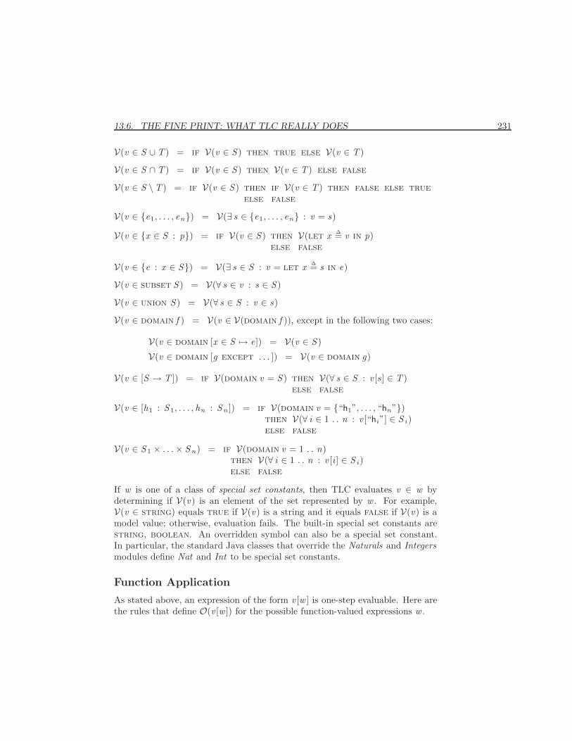
13.6. THE FINE PRINT: WHAT TLC REALLY DOES 231
V(v ∈ S ∪ T ) = if V(v ∈ S ) then true else V(v ∈ T )
V(v ∈ S ∩ T ) = if V(v ∈ S ) then V(v ∈ T ) else false
V(v ∈ S \T ) = if V(v ∈ S ) then if V(v ∈ T ) then false else trueelse false
V(v ∈ {e1, . . . , en}) = V(∃ s ∈ {e1, . . . , en} : v = s)
V(v ∈ {x ∈ S : p}) = if V(v ∈ S ) then V(let x ∆= v in p)else false
V(v ∈ {e : x ∈ S}) = V(∃ s ∈ S : v = let x ∆= s in e)
V(v ∈ subset S ) = V(∀ s ∈ v : s ∈ S )
V(v ∈ union S ) = V(∀ s ∈ S : v ∈ s)
V(v ∈ domain f ) = V(v ∈ V(domain f )), except in the following two cases:
V(v ∈ domain [x ∈ S 7→ e]) = V(v ∈ S )
V(v ∈ domain [g except . . . ]) = V(v ∈ domain g)
V(v ∈ [S → T ]) = if V(domain v = S ) then V(∀ s ∈ S : v [s ] ∈ T )else false
V(v ∈ [h1 : S 1, . . . , hn : Sn ]) = if V(domain v = {“h1”, . . . , “hn”})then V(∀ i ∈ 1 . . n : v [“hi”] ∈ S i)else false
V(v ∈ S 1 × . . .× Sn) = if V(domain v = 1 . . n)then V(∀ i ∈ 1 . . n : v [i ] ∈ S i)else false
If w is one of a class of special set constants, then TLC evaluates v ∈ w bydetermining if V(v) is an element of the set represented by w . For example,V(v ∈ string) equals true if V(v) is a string and it equals false if V(v) is amodel value; otherwise, evaluation fails. The built-in special set constants arestring, boolean. An overridden symbol can also be a special set constant.In particular, the standard Java classes that override the Naturals and Integersmodules define Nat and Int to be special set constants.
Function Application
As stated above, an expression of the form v [w ] is one-step evaluable. Here arethe rules that define O(v [w ]) for the possible function-valued expressions w .
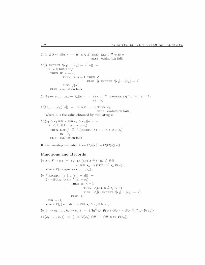
232 CHAPTER 13. THE TLC MODEL CHECKER
O([x ∈ S 7→ e][w ]) = if w ∈ S then let x ∆= w in eelse evaluation fails
O([f except ! [e1] . . . [en ] = d ][w ]) =if w ∈ domain f
then if w = e1
then if n = 1 then delse [f except ! [e2] . . . [en ] = d ]
else f [w ]else evaluation fails
O([h1 7→ e1, . . . , hn 7→ en ][w ]) = let j ∆= choose i ∈ 1 . . n : w = hi
in ej
O(〈e1, . . . , en 〉[w ]) = if u ∈ 1 . . n then eu
else evaluation fails ,where u is the value obtained by evaluating w .
O((s1 :> e1 @@ · · ·@@ sn :> en)[w ]) =if V(∃ i ∈ 1 . . n : w = s i)
then let j ∆= V(choose i ∈ 1 . . n : w = s i)in ej
else evaluation fails
If v is one-step evaluable, then O(v [w ]) = O(O(v)[w ]).
Functions and Records
V([x ∈ S 7→ e]) = (s1 :> (let x ∆= s1 in e) @@· · · @@ sn :> (let x ∆= sn in e)) ,
where V(S ) equals {s1, . . . , sn}.V([f except ! [e1] . . . [en ] = d ]) =
( · · ·@@ s i :> (if V(s i = ei)then if n = 1
then V(let @ ∆= t i in d)else V([t i except ! [e2] . . . [en ] = d ])
else t i@@ · · · ),
where V(f ) equals ( · · · @@ s i :> t i @@ · · · ).V([h1 7→ e1, . . . , hn 7→ en ]) = (“h1” :> V(e1) @@ · · · @@ “hn” :> V(en))
V(〈e1, . . . , en 〉) = (1 :> V(e1) @@ · · · @@ n :> V(en))
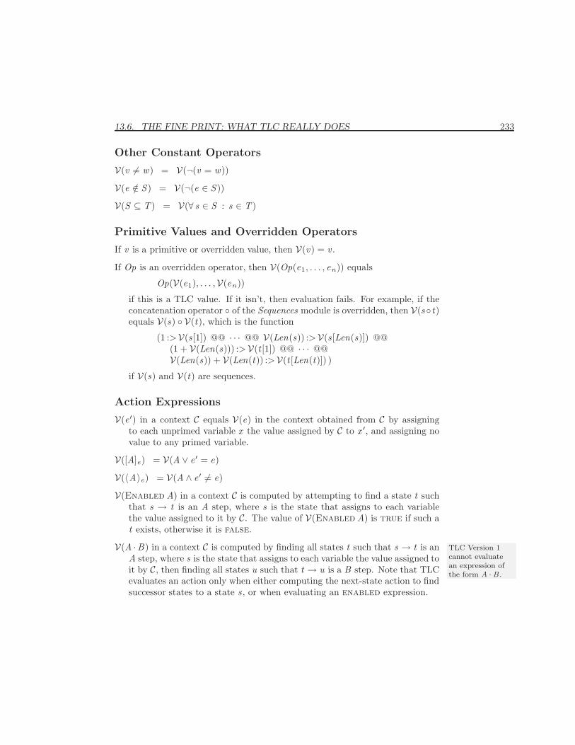
13.6. THE FINE PRINT: WHAT TLC REALLY DOES 233
Other Constant Operators
V(v 6= w) = V(¬(v = w))
V(e /∈ S ) = V(¬(e ∈ S ))
V(S ⊆ T ) = V(∀ s ∈ S : s ∈ T )
Primitive Values and Overridden Operators
If v is a primitive or overridden value, then V(v) = v .
If Op is an overridden operator, then V(Op(e1, . . . , en)) equals
Op(V(e1), . . . ,V(en))
if this is a TLC value. If it isn’t, then evaluation fails. For example, if theconcatenation operator ◦ of the Sequences module is overridden, then V(s ◦t)equals V(s) ◦ V(t), which is the function
(1 :>V(s [1]) @@ · · · @@ V(Len(s)) :>V(s [Len(s)]) @@(1 + V(Len(s))) :> V(t [1]) @@ · · · @@V(Len(s)) + V(Len(t)) :>V(t [Len(t)]) )
if V(s) and V(t) are sequences.
Action Expressions
V(e ′) in a context C equals V(e) in the context obtained from C by assigningto each unprimed variable x the value assigned by C to x ′, and assigning novalue to any primed variable.
V([A]e) = V(A ∨ e ′ = e)
V(〈A〉e) = V(A ∧ e ′ 6= e)
V(Enabled A) in a context C is computed by attempting to find a state t suchthat s → t is an A step, where s is the state that assigns to each variablethe value assigned to it by C. The value of V(Enabled A) is true if such at exists, otherwise it is false.
V(A ·B) in a context C is computed by finding all states t such that s → t is an TLC Version 1cannot evaluatean expression ofthe form A · B .
A step, where s is the state that assigns to each variable the value assigned toit by C, then finding all states u such that t → u is a B step. Note that TLCevaluates an action only when either computing the next-state action to findsuccessor states to a state s , or when evaluating an enabled expression.
234 CHAPTER 13. THE TLC MODEL CHECKER
13.6.4 Fingerprinting
The description of TLC’s computation in Section 13.2.6 is inaccurate in oneimportant respect. TLC does not actually keep the set of states R. Instead,it keeps the set of fingerprints of those states. A fingerprint of a state is a 64-bit value generated by a “hashing” function. Ideally, the probability that twodifferent states have the same fingerprint is 2−64, which is a very small number.
Rather than checking if a state s is in R, TLC checks if its fingerprint equalsthe fingerprint of a state already in R. With very high probability, that willbe true iff s is in R. However, it is possible for a collision to occur, meaningthat the fingerprint of s equals the fingerprint of some other state in R. If thishappens, TLC will not explore the successor states of s , and thus may not findall reachable states.
It is essentially impossible to do an accurate a posteriori calculation of theprobability that TLC did not check all reachable states because of a fingerprintcollision. If the probability that any two states have the same fingerprint is 2−64,then a simple calculation shows that if TLC generated n states with m distinctfingerprints, then the probability of a collision is about m ∗ (n − m) ∗ 2−64.However, the process of generating states is highly nonrandom, and no knownfingerprinting scheme can guarantee that the probability of any two distinctstates generated by TLC having the same fingerprint is actually 2−64. So, thisestimate is an optimistic one.
Another way to estimate the probability of collision is empirical. If therewas a collision, then it is likely that there was also a “near miss”. One estimateof the probability that there was a collision is the maximum value of 1/|f 1− f 2|over all pairs 〈f 1, f 2 〉 of distinct fingerprints generated by TLC for the statesthat it found.
TLC prints out both probability estimates when it finishes. You can usethese values to decide how much confidence to place in the completeness ofTLC’s exploration of the reachable states. You may wish to supplement TLC’smodel checking calculation with random simulation, which does not maintainthe set R and thus uses no fingerprinting.
Part IV
The TLA+ Language
235

237
This part of the book describes TLA+ in detail. Chapter 14 explains thesyntax; Chapters 15 and 16 explain the semantics; and Chapter 17 containsthe standard modules. Almost all of the TLA+ language has already beendescribed—mainly through examples. In fact, most of the language was de-scribed in Chapters 1–6. Here, we give a complete specification of the language.
A completely formal specification of TLA+ would consist of a formal defi-nition of the set of legal (syntactically well-formed) modules, and a precisely-defined meaning operator that assigns to every legal module M its mathematicalmeaning [[M ]]. Such a specification would be quite long and of limited interest.Instead, I have tried to provide a fairly informal specification that is detailedenough to show mathematically sophisticated readers how they could write acompletely formal one.
These chapters are heavy going, and only a few sophisticated readers willwant to read them completely. However, I hope they can serve as a referencemanual for anyone who reads or writes TLA+ specifications. If you have aquestion about the finer details of the syntax or the meaning of some part of thelanguage, you should be able to find the answer here.
Figures 13.9–13.16 on the next page through page 243 provide a tiny referencemanual. Figures 13.9–13.12 very briefly describe all the built-in operators ofTLA+. Figure 13.13 lists all the user-definable operator symbols, and indicateswhich ones are already used by the standard modules. Figure 13.14 gives theprecedence of the operators; it is explained in Section 14.2.1. Figure 13.15 listsall operators defined by the standard modules. Finally, Figure 13.16 shows howto type any symbol that doesn’t have an obvious ascii equivalent.
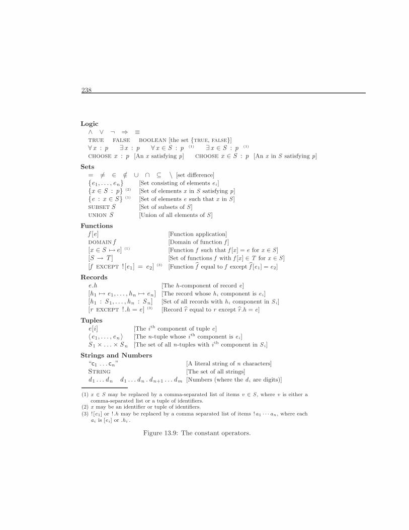
238
Logic∧ ∨ ¬ ⇒ ≡true false boolean [the set {true, false}]∀ x : p ∃ x : p ∀ x ∈ S : p (1) ∃ x ∈ S : p (1)
choose x : p [An x satisfying p] choose x ∈ S : p [An x in S satisfying p]
Sets= 6= ∈ /∈ ∪ ∩ ⊆ \ [set difference]
{e1, . . . , en} [Set consisting of elements e i ]
{x ∈ S : p} (2) [Set of elements x in S satisfying p]
{e : x ∈ S} (1) [Set of elements e such that x in S ]
subset S [Set of subsets of S ]
union S [Union of all elements of S ]
Functionsf [e] [Function application]
domain f [Domain of function f ]
[x ∈ S 7→ e] (1) [Function f such that f [x ] = e for x ∈ S ]
[S → T ] [Set of functions f with f [x ] ∈ T for x ∈ S ]
[f except ! [e1] = e2] (3) [Function f equal to f except f [e1] = e2]
Recordse.h [The h-component of record e]
[h1 7→ e1, . . . , hn 7→ en ] [The record whose h i component is e i ]
[h1 : S 1, . . . , hn : Sn ] [Set of all records with h i component in S i ]
[r except !.h = e] (3) [Record r equal to r except r .h = e]
Tuplese[i ] [The i th component of tuple e]
〈e1, . . . , en 〉 [The n-tuple whose i th component is e i ]
S 1 × . . .× Sn [The set of all n-tuples with i th component in S i ]
Strings and Numbers“c1 . . . cn” [A literal string of n characters]
String [The set of all strings]
d1 . . . dn d1 . . . dn . dn+1 . . . dm [Numbers (where the d i are digits)]
(1) x ∈ S may be replaced by a comma-separated list of items v ∈ S , where v is either acomma-separated list or a tuple of identifiers.
(2) x may be an identifier or tuple of identifiers.
(3) ![e1] or ! .h may be replaced by a comma separated list of items !a1 · · · an , where eachai is [ei ] or .hi .
Figure 13.9: The constant operators.
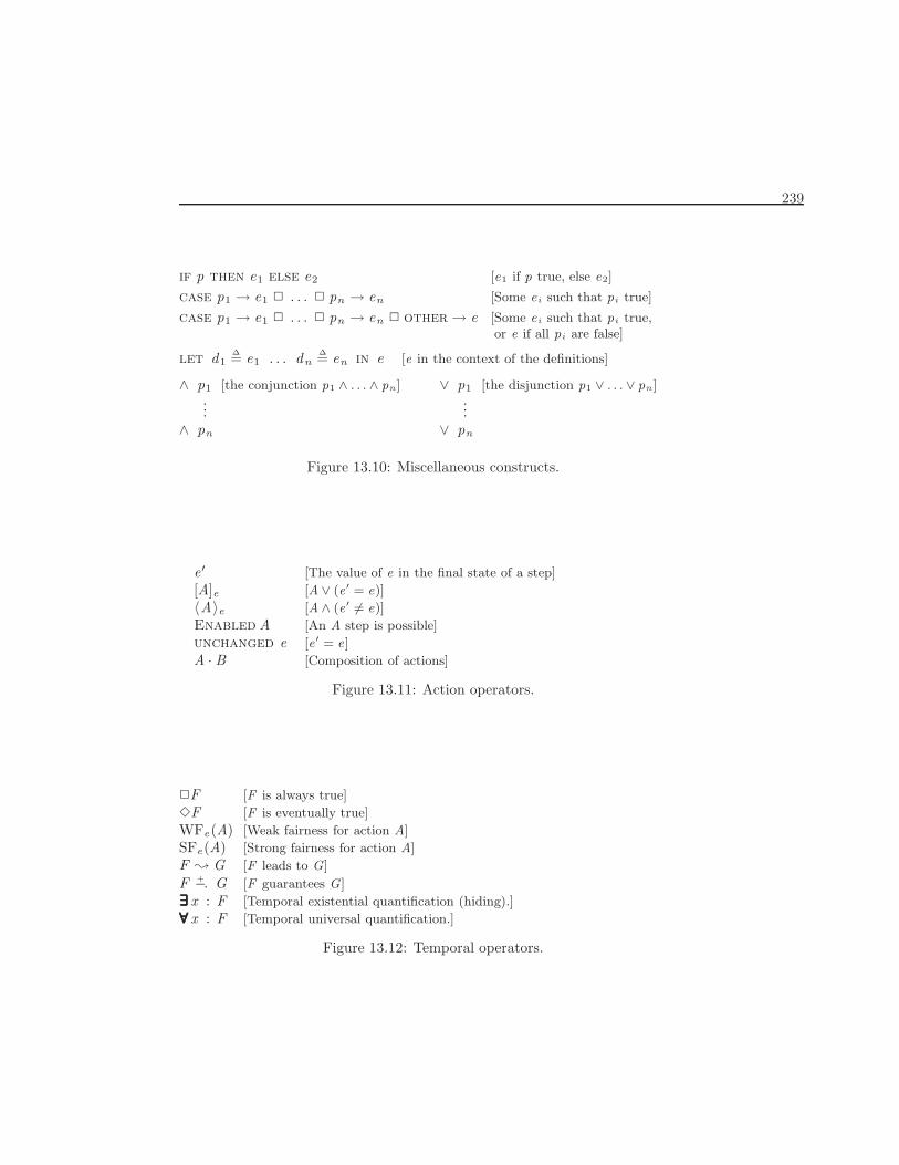
239
if p then e1 else e2 [e1 if p true, else e2]
case p1 → e1 2 . . . 2 pn → en [Some e i such that pi true]
case p1 → e1 2 . . . 2 pn → en 2 other→ e [Some e i such that pi true,or e if all pi are false]
let d1∆= e1 . . . dn
∆= en in e [e in the context of the definitions]
∧ p1
...∧ pn
[the conjunction p1 ∧ . . . ∧ pn ] ∨ p1
...∨ pn
[the disjunction p1 ∨ . . . ∨ pn ]
Figure 13.10: Miscellaneous constructs.
e ′ [The value of e in the final state of a step]
[A]e [A ∨ (e ′ = e)]
〈A〉e [A ∧ (e ′ 6= e)]
Enabled A [An A step is possible]
unchanged e [e ′ = e]
A · B [Composition of actions]
Figure 13.11: Action operators.
2F [F is always true]
3F [F is eventually true]
WFe(A) [Weak fairness for action A]
SFe(A) [Strong fairness for action A]
F ; G [F leads to G]
F +−. G [F guarantees G]
∃∃∃∃∃∃ x : F [Temporal existential quantification (hiding).]
∀∀∀∀∀∀ x : F [Temporal universal quantification.]
Figure 13.12: Temporal operators.
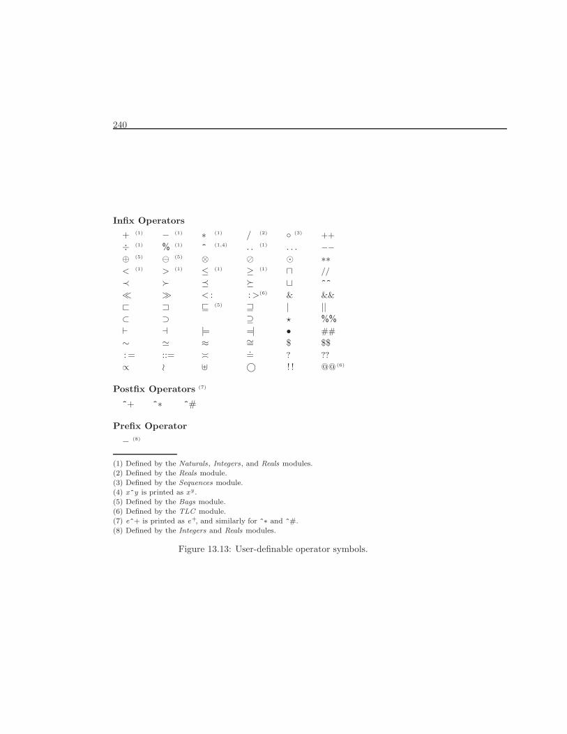
240
Infix Operators
+ (1) − (1) ∗ (1) / (2) ◦ (3) ++
÷ (1) % (1) ^ (1,4) . . (1) . . . −−⊕ (5) (5) ⊗ � � ∗∗< (1) > (1) ≤ (1) ≥ (1) u //
≺ � � � t ^^
� � < : : >(6) & &&
< = v (5) w | ||⊂ ⊃ ⊇ ? %%
` a |= =| • ##
∼ ' ≈ ∼= $ $$: = ::= � .= ? ??
∝ o ] © ! ! @@ (6)
Postfix Operators (7)
^+ ^∗ ^#
Prefix Operator
− (8)
(1) Defined by the Naturals, Integers, and Reals modules.
(2) Defined by the Reals module.
(3) Defined by the Sequences module.
(4) x^y is printed as xy .
(5) Defined by the Bags module.
(6) Defined by the TLC module.
(7) e^+ is printed as e+, and similarly for ^∗ and ^#.
(8) Defined by the Integers and Reals modules.
Figure 13.13: User-definable operator symbols.
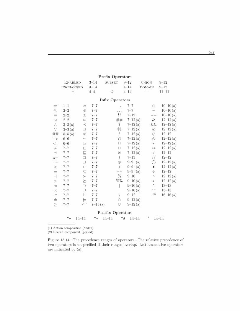
241
Prefix OperatorsEnabled 3–14
unchanged 3–14¬ 4–4
subset 9–122 4–143 4–14
union 9–12domain 9–12− 11–11
Infix Operators⇒ 1–1+−. 2–2≡ 2–2; 2–2∧ 3–3 (a)
∨ 3–3 (a)
@@ 5–5 (a)
: > 6–6< : 6–66= 7–7a 7–7
::= 7–7: = 7–7< 7–7= 7–7=| 7–7> 7–7≈ 7–7� 7–7∼= 7–7.= 7–7≥ 7–7
� 7–7∈ 7–7≤ 7–7� 7–7≺ 7–7� 7–7∝ 7–7∼ 7–7' 7–7< 7–7v 7–7= 7–7w 7–7⊂ 7–7⊆ 7–7� 7–7� 7–7⊃ 7–7⊇ 7–7` 7–7|= 7–7·(1) 7–13 (a)
. . 7–7. . . 7–7! ! 7–12
## 7–12 (a)
$ 7–12 (a)
$$ 7–12 (a)
? 7–12 (a)
?? 7–12 (a)
u 7–12 (a)
t 7–12 (a)
] 7–12 (a)
o 7–13⊕ 9–9 (a)
+ 9–9 (a)
++ 9–9 (a)
% 9–10%% 9–10 (a)
| 9–10 (a)
|| 9–10 (a)
\ 9–12∩ 9–12 (a)
∪ 9–12 (a)
10–10 (a)
− 10–10 (a)
−− 10–10 (a)
& 12–12 (a)
&& 12–12 (a)
� 12–12 (a)
� 12–12⊗ 12–12 (a)
∗ 12–12 (a)
∗∗ 12–12 (a)
/ 12–12// 12–12© 12–12 (a)
• 12–12 (a)
÷ 12–12◦ 12–12 (a)
? 12–12 (a)
^ 13–13^^ 13–13.(2) 16–16 (a)
Postfix Operators^+ 14–14 ^* 14–14 ^# 14–14 ′ 14–14
(1) Action composition (\cdot).
(2) Record component (period).
Figure 13.14: The precedence ranges of operators. The relative precedence oftwo operators is unspecified if their ranges overlap. Left-associative operatorsare indicated by (a).
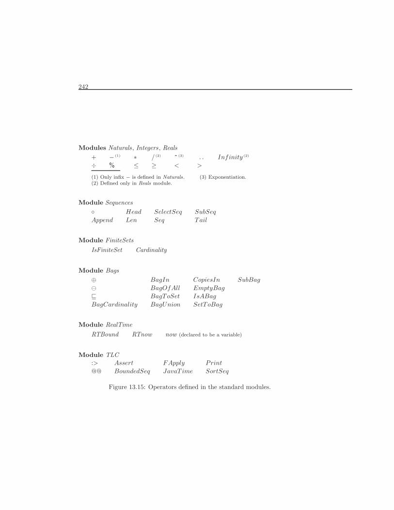
242
Modules Naturals , Integers , Reals+ − (1) ∗ / (2) ^ (3) . . Infinity (2)
÷ % ≤ ≥ < >
(1) Only infix − is defined in Naturals.(2) Defined only in Reals module.
(3) Exponentiation.
Module Sequences◦ Head SelectSeq SubSeq
Append Len Seq Tail
Module FiniteSetsIsFiniteSet Cardinality
Module Bags⊕ BagIn CopiesIn SubBag
BagOfAll EmptyBag
v BagToSet IsABag
BagCardinality BagUnion SetT oBag
Module RealTimeRTBound RTnow now (declared to be a variable)
Module TLC:> Assert FApply Print
@@ BoundedSeq JavaT ime SortSeq
Figure 13.15: Operators defined in the standard modules.
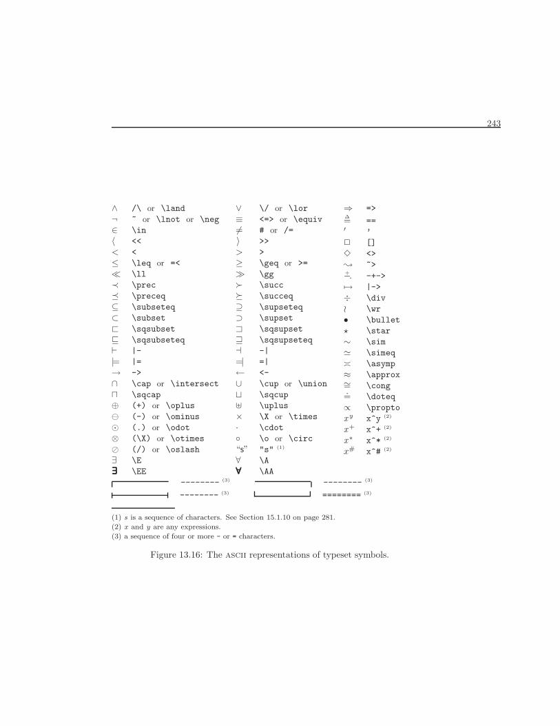
243
∧ /\ or \land¬ ~ or \lnot or \neg∈ \in〈 <<< <≤ \leq or =<� \ll≺ \prec� \preceq⊆ \subseteq⊂ \subset< \sqsubsetv \sqsubseteq` |-|= |=→ ->∩ \cap or \intersectu \sqcap⊕ (+) or \oplus (-) or \ominus� (.) or \odot⊗ (\X) or \otimes� (/) or \oslash∃ \E∃∃∃∃∃∃ \EE
∨ \/ or \lor≡ <=> or \equiv6= # or /=〉 >>> >≥ \geq or >=� \gg� \succ� \succeq⊇ \supseteq⊃ \supset= \sqsupsetw \sqsupseteqa -|=| =|← <-∪ \cup or \uniont \sqcup] \uplus× \X or \times· \cdot◦ \o or \circ“s” "s" (1)
∀ \A∀∀∀∀∀∀ \AA
⇒ =>∆= ==′ ’2 []3 <>; ~>+−. -+->7→ |->÷ \divo \wr• \bullet? \star∼ \sim' \simeq� \asymp≈ \approx∼= \cong.= \doteq∝ \proptox y x^y (2)
x+ x^+ (2)
x ∗ x^* (2)
x# x^# (2)
-------- (3) -------- (3)
-------- (3) ======== (3)
(1) s is a sequence of characters. See Section 15.1.10 on page 281.
(2) x and y are any expressions.
(3) a sequence of four or more - or = characters.
Figure 13.16: The ascii representations of typeset symbols.

244
Chapter 14
The Syntax of TLA+
The term syntax has two different usages, which I will somewhat arbitrarily at-tribute to mathematicians and computer scientists. A computer scientist wouldsay that 〈a, a 〉 is a syntactically correct TLA+ expression. A mathematicianwould say that the expression is syntactically correct iff it appears in a context inwhich a is defined or declared. A computer scientist would call this requirementa semantic rather than a syntactic condition. A mathematician would say that〈a, a 〉 is meaningless if a isn’t defined or declared, and one can’t talk about thesemantics of a meaningless expression.
This chapter describes the syntax of TLA+, in the computer scientist’s senseof syntax. (The “semantic” part of the syntax is specified in Chapters 15 and16.) TLA+ is designed to be easy for humans to read and write. In particu-lar, its syntax for expressions tries to capture some of the richness of ordinarymathematical notation. This makes a precise specification of the syntax rathercomplicated. Such a specification has been written in TLA+, but it is quite de-tailed and you probably don’t want to look at it unless you are writing a parserfor the language. This chapter gives a less formal description of the syntax thatshould answer any questions likely to arise in practice. Section 14.1 specifiesprecisely a simple grammar that ignores some aspects of the syntax such as op-erator precedence, indentation rules for ∧ and ∨ lists, and comments. Theseother aspects are explained informally in Section 14.2.1. Finally, Section 14.3lists the correspondence between the typed and typeset versions of symbols, aswell as all user-definable operator symbols.
245
246 CHAPTER 14. THE SYNTAX OF TLA+
14.1 The Simple Grammar
The simple grammar of TLA+ is described in BNF. Just for fun, this BNF gram- BNF, whichstands for Backus-Naur Form, is astandard way ofdescribing com-puter languages.
mar is specified in TLA+. Specifying a BNF grammar in TLA+ provides a nicelittle exercise in “mathematicizing” a simple concept. Moreover, it demonstratesthe flexibility of ordinary mathematics, as formalized in TLA+. The syntax ofTLA+ doesn’t permit us to write BNF grammars exactly the way you’re usedto seeing them, but we can come reasonably close.
Section 14.1.1 explains how to specify a BNF grammar. The BNF grammarfor TLA+ is specified in Section 14.1.2 as a TLA+ module, with comments thatdescribe how to read the TLA+ specification as an ordinary BNF grammar. Ifyou are familiar with BNF grammars and just want to learn the syntax of TLA+,you can skip directly to Section 14.1.2 (page 250).
14.1.1 BNF Grammars
Let’s start by reviewing BNF grammars. Consider the little language SE ofsimple expressions described by this BNF grammar:
expr ::= ident | expr op expr | ( expr ) | let def in exprdef ::= ident == expr
where op is some class of infix operators like +, and ident is some class ofidentifiers such as abc and x . The language SE contains expressions like
abc + (let x == y + abc in x ∗ x )
I will represent this expression as the sequence
〈 “abc”, “+”, “(”, “LET”, “x”, “==”, “y”, “+”, “abc”, “IN”, “x”, “*”, “x”, “)” 〉of strings. The strings such as “abc” and “+” appearing in this sequence areusually called lexemes. In general, a sequence of lexemes is called a sentence;and a set of sentences is called a language. So, we want to define the languageSE to consist of the set of all such sentences described by the BNF grammar.1
To represent a BNF grammar in TLA+, we must assign a mathematicalmeaning to nonterminal symbols like def , to terminal symbols like op, and tothe grammar’s two productions. The method that I find simplest is to let themeaning of a nonterminal symbol be the language that it generates. Thus, themeaning of expr is the language SE itself. I define a grammar to be a function Gsuch that, for any string “str”, the value of G[“str”] is the language generated by
1BNF grammars are also used to specify how an expression is parsed—for example thata + b ∗ c is parsed as a +(b ∗ c) rather than (a + b)∗ c. By considering the grammar to specifyonly a set of sentences, we are deliberately not capturing that use in our TLA+ representationof BNF grammars.
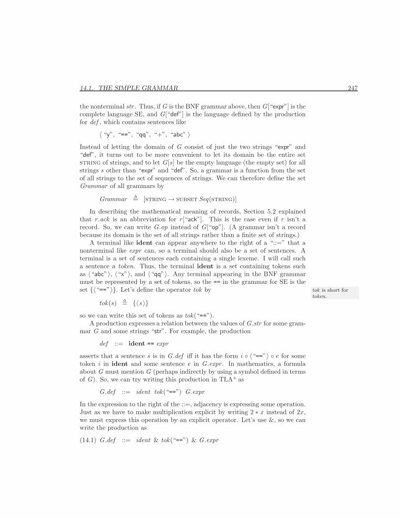
14.1. THE SIMPLE GRAMMAR 247
the nonterminal str . Thus, if G is the BNF grammar above, then G[“expr”] is thecomplete language SE, and G[“def”] is the language defined by the productionfor def , which contains sentences like
〈 “y”, “==”, “qq”, “+”, “abc” 〉Instead of letting the domain of G consist of just the two strings “expr” and“def”, it turns out to be more convenient to let its domain be the entire setstring of strings, and to let G[s ] be the empty language (the empty set) for allstrings s other than “expr” and “def”. So, a grammar is a function from the setof all strings to the set of sequences of strings. We can therefore define the setGrammar of all grammars by
Grammar ∆= [string→ subset Seq(string)]
In describing the mathematical meaning of records, Section 5.2 explainedthat r .ack is an abbreviation for r [“ack”]. This is the case even if r isn’t arecord. So, we can write G.op instead of G[“op”]. (A grammar isn’t a recordbecause its domain is the set of all strings rather than a finite set of strings.)
A terminal like ident can appear anywhere to the right of a “::=” that anonterminal like expr can, so a terminal should also be a set of sentences. Aterminal is a set of sentences each containing a single lexeme. I will call sucha sentence a token. Thus, the terminal ident is a set containing tokens suchas 〈“abc”〉, 〈“x”〉, and 〈“qq”〉. Any terminal appearing in the BNF grammarmust be represented by a set of tokens, so the == in the grammar for SE is theset {〈“==”〉}. Let’s define the operator tok by tok is short for
token.
tok(s) ∆= {〈s 〉}so we can write this set of tokens as tok(“==”).
A production expresses a relation between the values of G.str for some gram-mar G and some strings “str”. For example, the production
def ::= ident == expr
asserts that a sentence s is in G.def iff it has the form i ◦ 〈“==”〉 ◦ e for sometoken i in ident and some sentence e in G.expr . In mathematics, a formulaabout G must mention G (perhaps indirectly by using a symbol defined in termsof G). So, we can try writing this production in TLA+ as
G.def ::= ident tok(“==”) G.expr
In the expression to the right of the ::=, adjacency is expressing some operation.Just as we have to make multiplication explicit by writing 2 ∗ x instead of 2x ,we must express this operation by an explicit operator. Let’s use &, so we canwrite the production as
G.def ::= ident & tok(“==”) & G.expr(14.1)
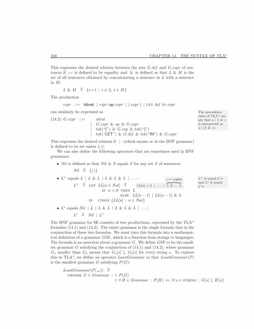
248 CHAPTER 14. THE SYNTAX OF TLA+
This expresses the desired relation between the sets G.def and G.expr of sen-tences if ::= is defined to be equality and & is defined so that L & M is theset of all sentences obtained by concatenating a sentence in L with a sentencein M :
L & M ∆= {s ◦ t : s ∈ L, t ∈ M }The production
expr ::= ident | expr op expr | ( expr ) | let def in expr
can similarly be expressed as The precedencerules of TLA+ im-ply that a | b & cis interpreted asa | (b & c).
G.expr ::= ident| G.expr & op & G.expr| tok(“(”) & G.exp & tok(“)”)| tok(“LET”) & G.def & tok(“IN”) & G.expr
(14.2)
This expresses the desired relation if | (which means or in the BNF grammar)is defined to be set union (∪).
We can also define the following operators that are sometimes used in BNFgrammars:
• Nil is defined so that Nil & S equals S for any set S of sentences:
Nil ∆= {〈 〉}• L+ equals L | L & L | L & L & L | . . . : L+ is typed L^+
and L∗ is typedL^*.L+ ∆= let LL[n ∈ Nat ] ∆= LL[n] = L | . . . |
n+1 copies︷ ︸︸ ︷L & . . .L .
if n = 0 then Lelse LL[n − 1] | LL[n − 1] & L
in union {LL[n] : n ∈ Nat}• L∗ equals Nil | L | L & L | L & L & L | . . . :
L∗ ∆= Nil | L+
The BNF grammar for SE consists of two productions, expressed by the TLA+
formulas (14.1) and (14.2). The entire grammar is the single formula that is theconjunction of these two formulas. We must turn this formula into a mathemat-ical definition of a grammar GSE , which is a function from strings to languages.The formula is an assertion about a grammar G. We define GSE to be the small-est grammar G satisfying the conjunction of (14.1) and (14.2), where grammarG1 smaller than G2 means that G1[s ] ⊆ G2[s ] for every string s . To expressthis in TLA+, we define an operator LeastGrammar so that LeastGrammar(P)is the smallest grammar G satisfying P(G):
LeastGrammar(P( )) ∆=choose G ∈ Grammar : ∧ P(G)
∧ ∀H ∈ Grammar : P(H ) ⇒ (∀ s ∈ string : G[s ] ⊆ H [s ])
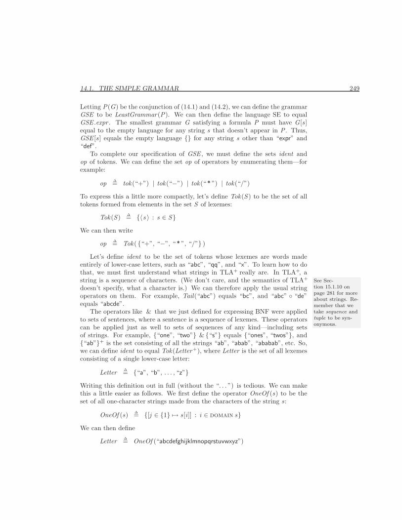
14.1. THE SIMPLE GRAMMAR 249
Letting P(G) be the conjunction of (14.1) and (14.2), we can define the grammarGSE to be LeastGrammar(P). We can then define the language SE to equalGSE .expr . The smallest grammar G satisfying a formula P must have G[s ]equal to the empty language for any string s that doesn’t appear in P . Thus,GSE [s ] equals the empty language {} for any string s other than “expr” and“def”.
To complete our specification of GSE , we must define the sets ident andop of tokens. We can define the set op of operators by enumerating them—forexample:
op ∆= tok(“+”) | tok(“−”) | tok(“ * ”) | tok(“/”)
To express this a little more compactly, let’s define Tok(S ) to be the set of alltokens formed from elements in the set S of lexemes:
Tok(S ) ∆= {〈s 〉 : s ∈ S}We can then write
op ∆= Tok( {“+”, “−”, “ * ”, “/”} )
Let’s define ident to be the set of tokens whose lexemes are words madeentirely of lower-case letters, such as “abc”, “qq”, and “x”. To learn how to dothat, we must first understand what strings in TLA+ really are. In TLA+, astring is a sequence of characters. (We don’t care, and the semantics of TLA+ See Sec-
tion 15.1.10 onpage 281 for moreabout strings. Re-member that wetake sequence andtuple to be syn-onymous.
doesn’t specify, what a character is.) We can therefore apply the usual stringoperators on them. For example, Tail(“abc”) equals “bc”, and “abc” ◦ “de”equals “abcde”.
The operators like & that we just defined for expressing BNF were appliedto sets of sentences, where a sentence is a sequence of lexemes. These operatorscan be applied just as well to sets of sequences of any kind—including setsof strings. For example, {“one”, “two”} & {“s”} equals {“ones”, “twos”}, and{“ab”}+ is the set consisting of all the strings “ab”, “abab”, “ababab”, etc. So,we can define ident to equal Tok(Letter+), where Letter is the set of all lexemesconsisting of a single lower-case letter:
Letter ∆= {“a”, “b”, . . . , “z”}Writing this definition out in full (without the “. . . ”) is tedious. We can makethis a little easier as follows. We first define the operator OneOf (s) to be theset of all one-character strings made from the characters of the string s :
OneOf (s) ∆= {[j ∈ {1} 7→ s [i ]] : i ∈ domain s}We can then define
Letter ∆= OneOf (“abcdefghijklmnopqrstuvwxyz”)
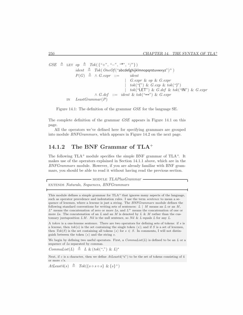
250 CHAPTER 14. THE SYNTAX OF TLA+
GSE ∆= let op ∆= Tok( {“+”, “−”, “*”, “/”} )ident ∆= Tok(OneOf (“abcdefghijklmnopqrstuvwxyz”)+ )P(G) ∆= ∧ G.expr ::= ident
| G.expr & op & G.expr| tok(“(”) & G.exp & tok(“)”)| tok(“LET”) & G.def & tok(“IN”) & G.expr
∧ G.def ::= ident & tok(“==”) & G.exprin LeastGrammar(P)
Figure 14.1: The definition of the grammar GSE for the language SE.
The complete definition of the grammar GSE appears in Figure 14.1 on thispage.
All the operators we’ve defined here for specifying grammars are groupedinto module BNFGrammars , which appears in Figure 14.2 on the next page.
14.1.2 The BNF Grammar of TLA+
The following TLA+ module specifies the simple BNF grammar of TLA+. Itmakes use of the operators explained in Section 14.1.1 above, which are in theBNFGrammars module. However, if you are already familiar with BNF gram-mars, you should be able to read it without having read the previous section.
module TLAPlusGrammarextends Naturals, Sequences, BNFGrammars
This module defines a simple grammar for TLA+ that ignores many aspects of the language,such as operator precedence and indentation rules. I use the term sentence to mean a se-quence of lexemes, where a lexeme is just a string. The BNFGrammars module defines thefollowing standard conventions for writing sets of sentences: L | M means an L or an M ,L∗ means the concatenation of zero or more Ls, and L+ means the concatenation of one ormore Ls. The concatenation of an L and an M is denoted by L & M rather than the cus-tomary juxtaposition LM . Nil is the null sentence, so Nil & L equals L for any L.
A token is a one-lexeme sentence. There are two operators for defining sets of tokens: if s isa lexeme, then tok(s) is the set containing the single token 〈s 〉; and if S is a set of lexemes,then Tok(S) is the set containing all tokens 〈s 〉 for s ∈ S . In comments, I will not distin-guish between the token 〈s 〉 and the string s.
We begin by defining two useful operators. First, a CommaList(L) is defined to be an L or asequence of Ls separated by commas.
CommaList(L) ∆= L & (tok(“,”) & L)∗
Next, if c is a character, then we define AtLeast4(“c”) to be the set of tokens consisting of 4or more c’s.
AtLeast4(s) ∆= Tok({s ◦ s ◦ s} & {s}+)
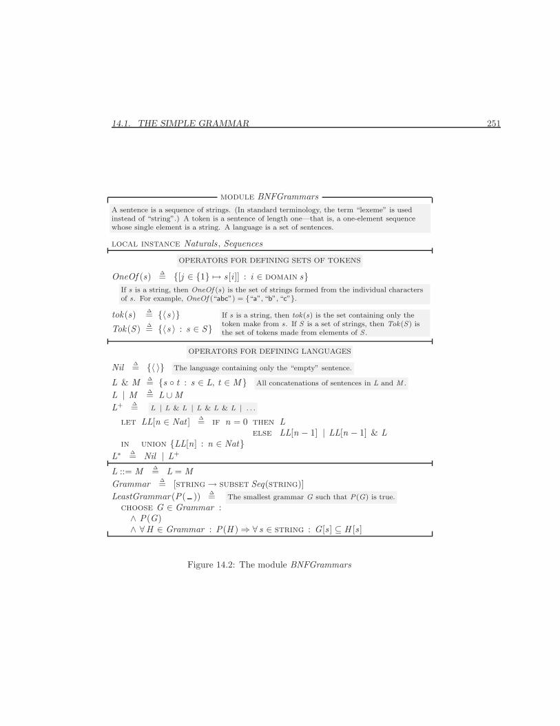
14.1. THE SIMPLE GRAMMAR 251
module BNFGrammarsA sentence is a sequence of strings. (In standard terminology, the term “lexeme” is usedinstead of “string”.) A token is a sentence of length one—that is, a one-element sequencewhose single element is a string. A language is a set of sentences.
local instance Naturals , Sequences
OPERATORS FOR DEFINING SETS OF TOKENS
OneOf (s) ∆= {[j ∈ {1} 7→ s [i ]] : i ∈ domain s}If s is a string, then OneOf (s) is the set of strings formed from the individual charactersof s. For example, OneOf (“abc”) = {“a”, “b”, “c”}.
tok(s) ∆= {〈s 〉}Tok(S ) ∆= {〈s 〉 : s ∈ S}
If s is a string, then tok(s) is the set containing only thetoken make from s. If S is a set of strings, then Tok(S) isthe set of tokens made from elements of S .
OPERATORS FOR DEFINING LANGUAGES
Nil ∆= {〈 〉} The language containing only the “empty” sentence.
L & M ∆= {s ◦ t : s ∈ L, t ∈ M } All concatenations of sentences in L and M .
L | M ∆= L ∪ML+ ∆= L | L & L | L & L & L | . . .
let LL[n ∈ Nat ] ∆= if n = 0 then Lelse LL[n − 1] | LL[n − 1] & L
in union {LL[n] : n ∈ Nat}L∗ ∆= Nil | L+
L ::= M ∆= L = MGrammar ∆= [string→ subset Seq(string)]LeastGrammar(P( )) ∆= The smallest grammar G such that P(G) is true.
choose G ∈ Grammar :∧ P(G)∧ ∀H ∈ Grammar : P(H )⇒ ∀ s ∈ string : G[s ] ⊆ H [s ]
Figure 14.2: The module BNFGrammars
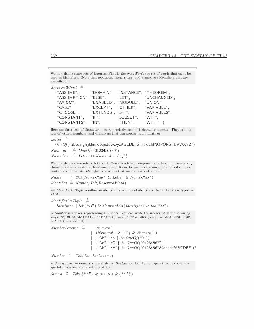
252 CHAPTER 14. THE SYNTAX OF TLA+
We now define some sets of lexemes. First is ReservedWord , the set of words that can’t beused as identifiers. (Note that boolean, true, false, and string are identifiers that arepredefined.)
ReservedWord ∆={“ASSUME”, “DOMAIN”, “INSTANCE”, “THEOREM”,“ASSUMPTION”, “ELSE”, “LET”, “UNCHANGED”,“AXIOM”, “ENABLED”, “MODULE”, “UNION”,“CASE”, “EXCEPT”, “OTHER”, “VARIABLE”,“CHOOSE”, “EXTENDS”, “SF_”, “VARIABLES”,“CONSTANT”, “IF”, “SUBSET”, “WF_”,“CONSTANTS”, “IN”, “THEN”, “WITH” }
Here are three sets of characters—more precisely, sets of 1-character lexemes. They are thesets of letters, numbers, and characters that can appear in an identifier.
Letter ∆=OneOf (“abcdefghijklmnopqrstuvwxyzABCDEFGHIJKLMNOPQRSTUVWXYZ”)
Numeral ∆= OneOf (“0123456789”)NameChar ∆= Letter ∪ Numeral ∪ {“_”}We now define some sets of tokens. A Name is a token composed of letters, numbers, and _
characters that contains at least one letter. It can be used as the name of a record compo-nent or a module. An Identifier is a Name that isn’t a reserved word.
Name ∆= Tok(NameChar∗ & Letter & NameChar∗)Identifier ∆= Name \Tok(ReservedWord)
An IdentifierOrTuple is either an identifier or a tuple of identifiers. Note that 〈 〉 is typed as<< >>.
IdentifierOrTuple ∆=Identifier | tok(“<<”) & CommaList(Identifier) & tok(“>>”)
A Number is a token representing a number. You can write the integer 63 in the followingways: 63, 63.00, \b111111 or \B111111 (binary), \o77 or \O77 (octal), or \h3f, \H3f, \h3F,or \H3F (hexadecimal).
NumberLexeme ∆= Numeral+
| (Numeral∗ & {“.”} & Numeral+)| {“\b”, “\b”} & OneOf (“01”)+
| {“\o”, “\O”} & OneOf (“01234567”)+
| {“\h”, “\H”} & OneOf (“0123456789abcdefABCDEF”)+
Number ∆= Tok(NumberLexeme)
A String token represents a literal string. See Section 15.1.10 on page 281 to find out howspecial characters are typed in a string.
String ∆= Tok( {“ " ”} & string & {“ " ”} )
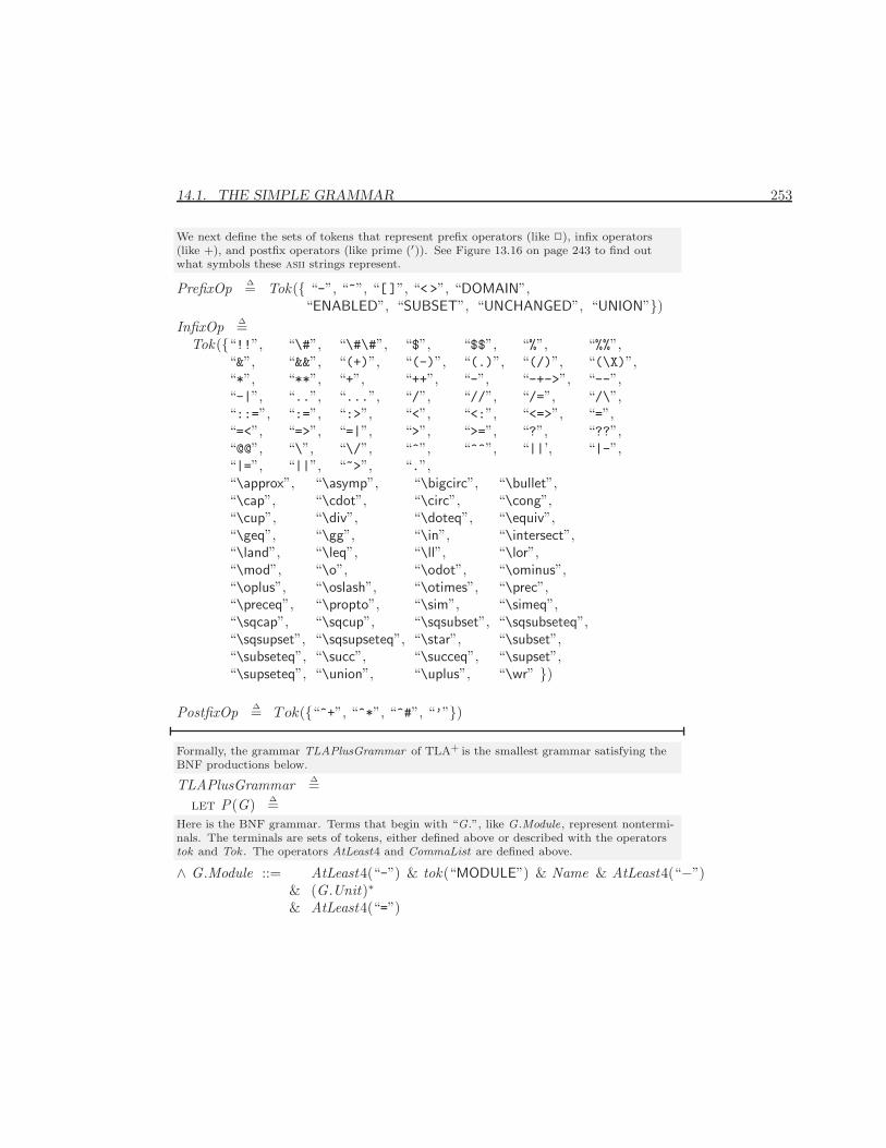
14.1. THE SIMPLE GRAMMAR 253
We next define the sets of tokens that represent prefix operators (like 2), infix operators(like +), and postfix operators (like prime (′)). See Figure 13.16 on page 243 to find outwhat symbols these asii strings represent.
PrefixOp ∆= Tok({ “-”, “~”, “[ ]”, “< >”, “DOMAIN”,“ENABLED”, “SUBSET”, “UNCHANGED”, “UNION”})
InfixOp ∆=Tok({“!!”, “\#”, “\#\#”, “$”, “$$”, “%”, “%%”,
“&”, “&&”, “(+)”, “(-)”, “(.)”, “(/)”, “(\X)”,“*”, “**”, “+”, “++”, “-”, “-+->”, “--”,“-|”, “..”, “...”, “/”, “//”, “/=”, “/\”,“::=”, “:=”, “:>”, “<”, “<:”, “<=>”, “=”,“=<”, “=>”, “=|”, “>”, “>=”, “?”, “??”,“@@”, “\”, “\/”, “^”, “^^”, “||’, “|-”,“|=”, “||”, “~>”, “.”,“\approx”, “\asymp”, “\bigcirc”, “\bullet”,“\cap”, “\cdot”, “\circ”, “\cong”,“\cup”, “\div”, “\doteq”, “\equiv”,“\geq”, “\gg”, “\in”, “\intersect”,“\land”, “\leq”, “\ll”, “\lor”,“\mod”, “\o”, “\odot”, “\ominus”,“\oplus”, “\oslash”, “\otimes”, “\prec”,“\preceq”, “\propto”, “\sim”, “\simeq”,“\sqcap”, “\sqcup”, “\sqsubset”, “\sqsubseteq”,“\sqsupset”, “\sqsupseteq”, “\star”, “\subset”,“\subseteq”, “\succ”, “\succeq”, “\supset”,“\supseteq”, “\union”, “\uplus”, “\wr” })
PostfixOp ∆= Tok({“^+”, “^*”, “^#”, “’”})
Formally, the grammar TLAPlusGrammar of TLA+ is the smallest grammar satisfying theBNF productions below.
TLAPlusGrammar ∆=let P(G) ∆=
Here is the BNF grammar. Terms that begin with “G.”, like G.Module, represent nontermi-nals. The terminals are sets of tokens, either defined above or described with the operatorstok and Tok . The operators AtLeast4 and CommaList are defined above.
∧ G.Module ::= AtLeast4(“-”) & tok(“MODULE”) & Name & AtLeast4(“−”)& (G.Unit)∗
& AtLeast4(“=”)
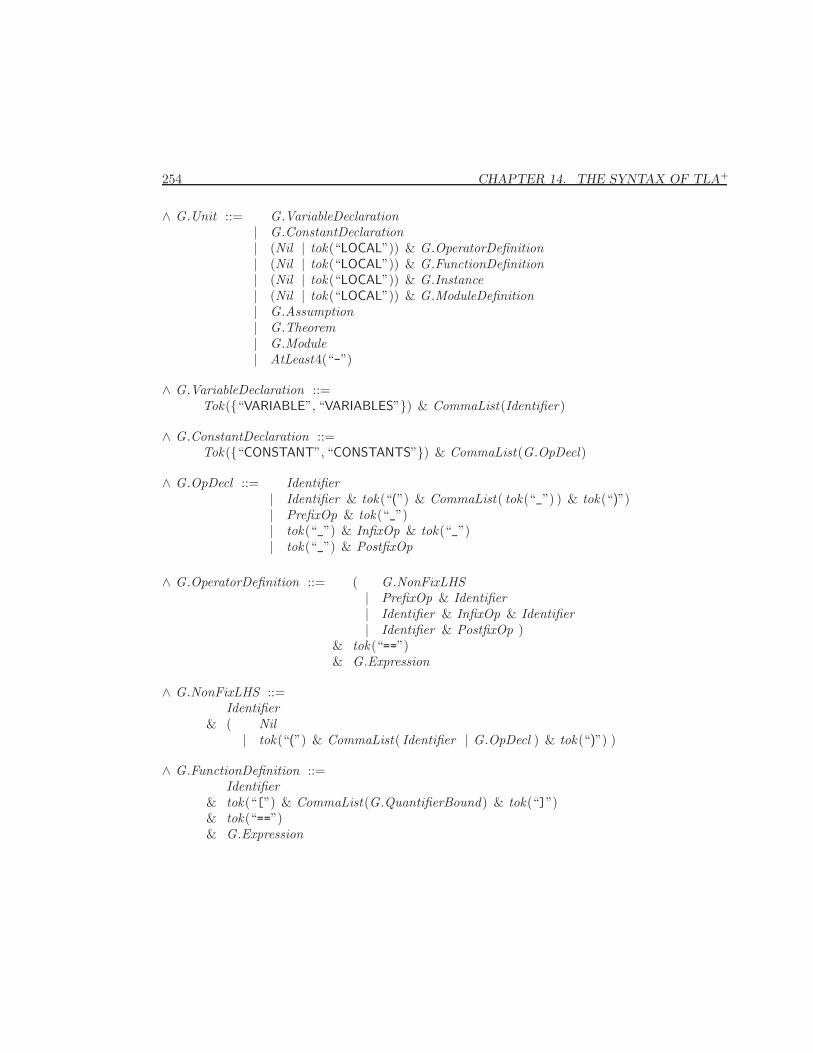
254 CHAPTER 14. THE SYNTAX OF TLA+
∧ G.Unit ::= G.VariableDeclaration| G.ConstantDeclaration| (Nil | tok(“LOCAL”)) & G.OperatorDefinition| (Nil | tok(“LOCAL”)) & G.FunctionDefinition| (Nil | tok(“LOCAL”)) & G.Instance| (Nil | tok(“LOCAL”)) & G.ModuleDefinition| G.Assumption| G.Theorem| G.Module| AtLeast4(“-”)
∧ G.VariableDeclaration ::=Tok({“VARIABLE”, “VARIABLES”}) & CommaList(Identifier)
∧ G.ConstantDeclaration ::=Tok({“CONSTANT”, “CONSTANTS”}) & CommaList(G.OpDecl)
∧ G.OpDecl ::= Identifier| Identifier & tok(“(”) & CommaList( tok(“_”) ) & tok(“)”)| PrefixOp & tok(“_”)| tok(“_”) & InfixOp & tok(“_”)| tok(“_”) & PostfixOp
∧ G.OperatorDefinition ::= ( G.NonFixLHS| PrefixOp & Identifier| Identifier & InfixOp & Identifier| Identifier & PostfixOp )
& tok(“==”)& G.Expression
∧ G.NonFixLHS ::=Identifier
& ( Nil| tok(“(”) & CommaList( Identifier | G.OpDecl ) & tok(“)”) )
∧ G.FunctionDefinition ::=Identifier
& tok(“[”) & CommaList(G.QuantifierBound) & tok(“]”)& tok(“==”)& G.Expression
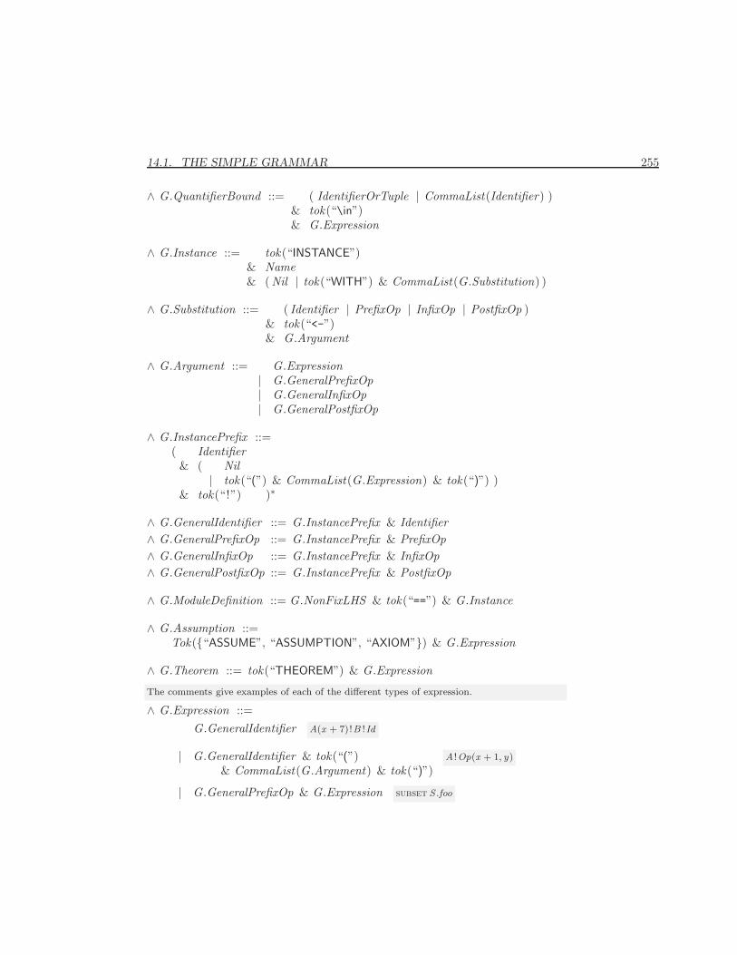
14.1. THE SIMPLE GRAMMAR 255
∧ G.QuantifierBound ::= ( IdentifierOrTuple | CommaList(Identifier) )& tok(“\in”)& G.Expression
∧ G.Instance ::= tok(“INSTANCE”)& Name& (Nil | tok(“WITH”) & CommaList(G.Substitution) )
∧ G.Substitution ::= ( Identifier | PrefixOp | InfixOp | PostfixOp )& tok(“<-”)& G.Argument
∧ G.Argument ::= G.Expression| G.GeneralPrefixOp| G.GeneralInfixOp| G.GeneralPostfixOp
∧ G.InstancePrefix ::=( Identifier& ( Nil
| tok(“(”) & CommaList(G.Expression) & tok(“)”) )& tok(“!”) )∗
∧ G.GeneralIdentifier ::= G.InstancePrefix & Identifier∧ G.GeneralPrefixOp ::= G.InstancePrefix & PrefixOp∧ G.GeneralInfixOp ::= G.InstancePrefix & InfixOp∧ G.GeneralPostfixOp ::= G.InstancePrefix & PostfixOp
∧ G.ModuleDefinition ::= G.NonFixLHS & tok(“==”) & G.Instance
∧ G.Assumption ::=Tok({“ASSUME”, “ASSUMPTION”, “AXIOM”}) & G.Expression
∧ G.Theorem ::= tok(“THEOREM”) & G.Expression
The comments give examples of each of the different types of expression.
∧ G.Expression ::=G.GeneralIdentifier A(x + 7)!B !Id
| G.GeneralIdentifier & tok(“(”)& CommaList(G.Argument) & tok(“)”)
A !Op(x + 1, y)
| G.GeneralPrefixOp & G.Expression subset S .foo
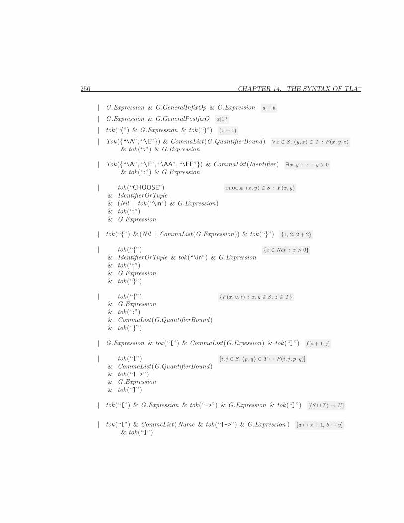
256 CHAPTER 14. THE SYNTAX OF TLA+
| G.Expression & G.GeneralInfixOp & G.Expression a + b
| G.Expression & G.GeneralPostfixO x [1]′
| tok(“(”) & G.Expression & tok(“)”) (x + 1)
| Tok({“\A”, “\E”}) & CommaList(G.QuantifierBound)& tok(“:”) & G.Expression
∀ x ∈ S , 〈y , z 〉 ∈ T : F (x , y , z)
| Tok({“\A”, “\E”, “\AA”, “\EE”}) & CommaList(Identifier)& tok(“:”) & G.Expression
∃ x , y : x + y > 0
| tok(“CHOOSE”)& IdentifierOrTuple& (Nil | tok(“\in”) & G.Expression)& tok(“:”)& G.Expression
choose 〈x , y 〉 ∈ S : F (x , y)
| tok(“{”) & (Nil | CommaList(G.Expression)) & tok(“}”) {1, 2, 2 + 2}
| tok(“{”)& IdentifierOrTuple & tok(“\in”) & G.Expression& tok(“:”)& G.Expression& tok(“}”)
{x ∈ Nat : x > 0}
| tok(“{”)& G.Expression& tok(“:”)& CommaList(G.QuantifierBound)& tok(“}”)
{F (x , y , z) : x , y ∈ S , z ∈ T}
| G.Expression & tok(“[”) & CommaList(G.Expession) & tok(“]”) f [i + 1, j ]
| tok(“[”)& CommaList(G.QuantifierBound)& tok(“|->”)& G.Expression& tok(“]”)
[i , j ∈ S , 〈p, q 〉 ∈ T 7→ F (i , j , p, q)]
| tok(“[”) & G.Expression & tok(“->”) & G.Expression & tok(“]”) [(S ∪ T ) → U ]
| tok(“[”) & CommaList(Name & tok(“|->”) & G.Expression )& tok(“]”)
[a 7→ x + 1, b 7→ y ]
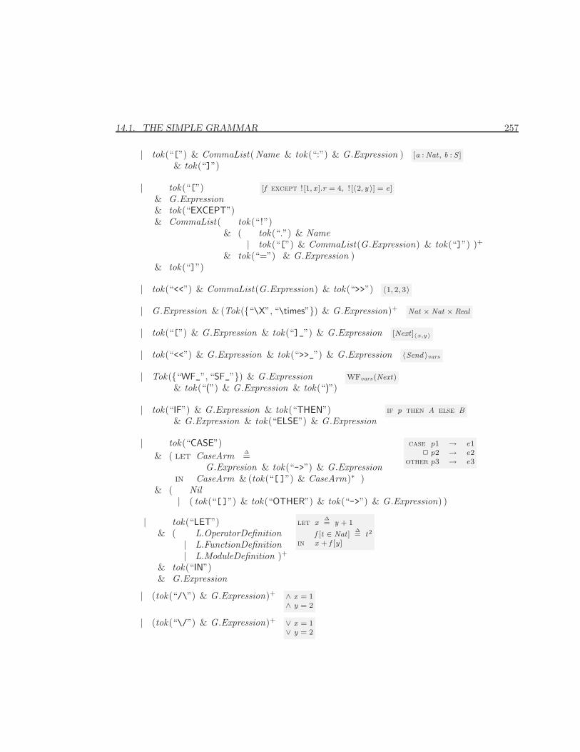
14.1. THE SIMPLE GRAMMAR 257
| tok(“[”) & CommaList(Name & tok(“:”) & G.Expression )& tok(“]”)
[a : Nat , b : S ]
| tok(“[”) [f except ! [1, x ].r = 4, ! [〈2, y 〉] = e]
& G.Expression& tok(“EXCEPT”)& CommaList( tok(“!”)
& ( tok(“.”) & Name| tok(“[”) & CommaList(G.Expression) & tok(“]”) )+
& tok(“=”) & G.Expression )& tok(“]”)
| tok(“<<”) & CommaList(G.Expression) & tok(“>>”) 〈1, 2, 3〉
| G.Expression & (Tok({“\X”, “\times”}) & G.Expression)+ Nat × Nat × Real
| tok(“[”) & G.Expression & tok(“]_”) & G.Expression [Next ]〈x ,y 〉
| tok(“<<”) & G.Expression & tok(“>>_”) & G.Expression 〈Send 〉vars
| Tok({“WF_”, “SF_”}) & G.Expression& tok(“(”) & G.Expression & tok(“)”)
WFvars(Next)
| tok(“IF”) & G.Expression & tok(“THEN”)& G.Expression & tok(“ELSE”) & G.Expression
if p then A else B
| tok(“CASE”) case p1 → e12 p2 → e2
other p3 → e3& ( let CaseArm ∆=
G.Expresion & tok(“->”) & G.Expressionin CaseArm & (tok(“[ ]”) & CaseArm)∗ )
& ( Nil| ( tok(“[ ]”) & tok(“OTHER”) & tok(“->”) & G.Expression) )
| tok(“LET”)& ( L.OperatorDefinition
| L.FunctionDefinition| L.ModuleDefinition )+
& tok(“IN”)& G.Expression
let x∆= y + 1
f [t ∈ Nat ]∆= t2
in x + f [y ]
| (tok(“/\”) & G.Expression)+ ∧ x = 1∧ y = 2
| (tok(“\/”) & G.Expression)+ ∨ x = 1∨ y = 2
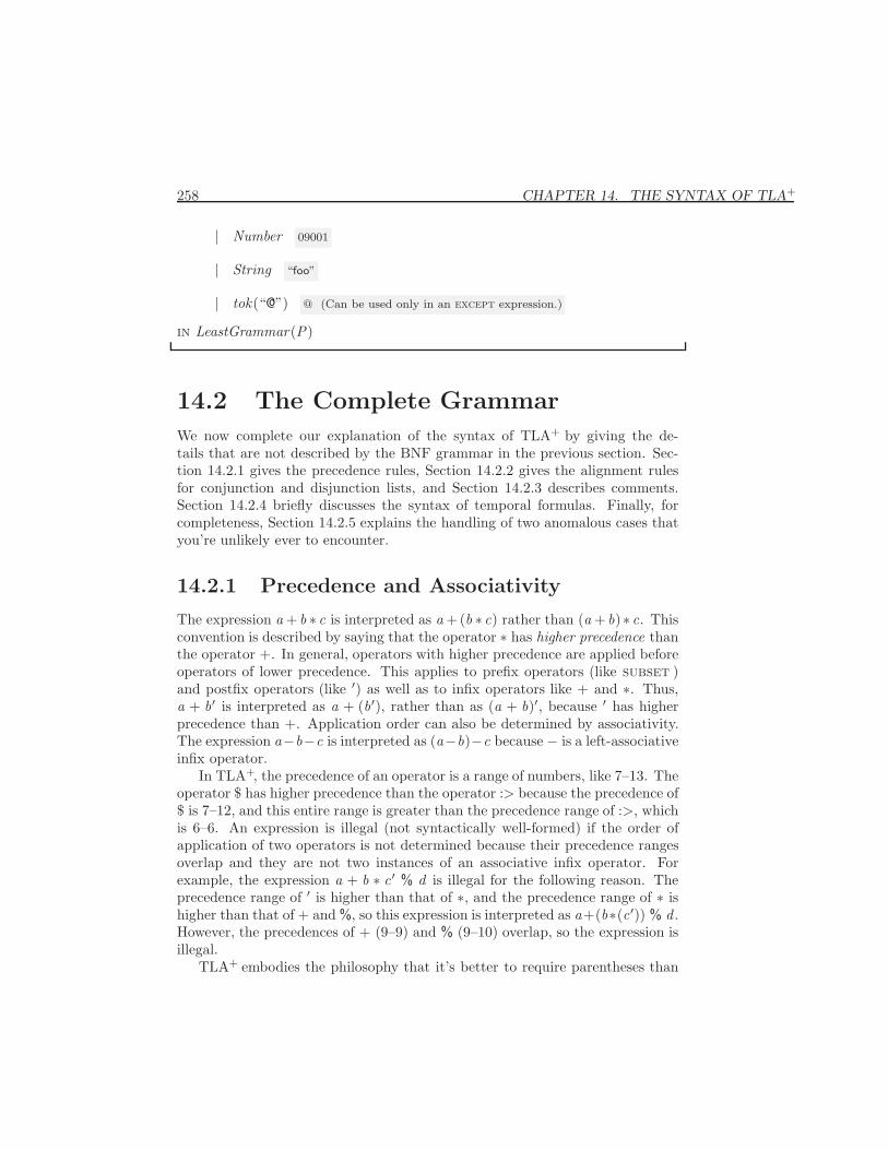
258 CHAPTER 14. THE SYNTAX OF TLA+
| Number 09001
| String “foo”
| tok(“@”) @ (Can be used only in an except expression.)
in LeastGrammar(P)
14.2 The Complete Grammar
We now complete our explanation of the syntax of TLA+ by giving the de-tails that are not described by the BNF grammar in the previous section. Sec-tion 14.2.1 gives the precedence rules, Section 14.2.2 gives the alignment rulesfor conjunction and disjunction lists, and Section 14.2.3 describes comments.Section 14.2.4 briefly discusses the syntax of temporal formulas. Finally, forcompleteness, Section 14.2.5 explains the handling of two anomalous cases thatyou’re unlikely ever to encounter.
14.2.1 Precedence and Associativity
The expression a + b ∗ c is interpreted as a +(b ∗ c) rather than (a + b)∗ c. Thisconvention is described by saying that the operator ∗ has higher precedence thanthe operator +. In general, operators with higher precedence are applied beforeoperators of lower precedence. This applies to prefix operators (like subset )and postfix operators (like ′) as well as to infix operators like + and ∗. Thus,a + b′ is interpreted as a + (b′), rather than as (a + b)′, because ′ has higherprecedence than +. Application order can also be determined by associativity.The expression a−b−c is interpreted as (a−b)−c because − is a left-associativeinfix operator.
In TLA+, the precedence of an operator is a range of numbers, like 7–13. Theoperator $ has higher precedence than the operator :> because the precedence of$ is 7–12, and this entire range is greater than the precedence range of :>, whichis 6–6. An expression is illegal (not syntactically well-formed) if the order ofapplication of two operators is not determined because their precedence rangesoverlap and they are not two instances of an associative infix operator. Forexample, the expression a + b ∗ c′ % d is illegal for the following reason. Theprecedence range of ′ is higher than that of ∗, and the precedence range of ∗ ishigher than that of + and %, so this expression is interpreted as a+(b∗(c′)) % d .However, the precedences of + (9–9) and % (9–10) overlap, so the expression isillegal.
TLA+ embodies the philosophy that it’s better to require parentheses than
14.2. THE COMPLETE GRAMMAR 259
to allow expressions that could be easily be misinterpreted. Thus, ∗ and / haveoverlapping precedence, making an expression like a/b ∗ c illegal. (This alsomakes a ∗ b/c illegal, even though (a ∗ b)/c and a ∗ (b/c) happen to be equalwhen ∗ and / have their usual definitions.) Unconventional operators like $ havewide precedence ranges for safety. But, even when the precedence rules implythat parentheses aren’t needed, it’s often a good idea to use them anyway if youthink there’s any chance that a reader might not understand how an expressionis parsed.
Figure 13.14 on page 241 gives the precedence ranges of all operators andtells which infix operators are left associative. (No TLA+ operators are rightassociative.) Below are some additional precedence rules not covered by theoperator precedence ranges.
Function Application
Function application has higher precedence than any operator. Thus, a + b[c]′
is interpreted as a + (b[c])′. (This in turn is interpreted as a + ((b[c])′), sincethe ′ operator has higher precedence than +.)
Cartesian Products
In the Cartesian product construct, × (typed as \X or \times) acts somewhatlike an associative infix operator with precedence range 9–12. Thus, A×B ⊆ Cis interpreted as (A × B) ⊆ C , rather than as A × (B ⊆ C ). However, × ispart of a special construct, not an infix operator. For example, the three setsA× B × C , (A× B)× C , and A× (B × C ) are all different:
A× B × C = {〈a, b, c 〉 : a ∈ A, b ∈ B , c ∈ C}(A× B)× C = {〈〈a, b 〉, c 〉 : a ∈ A, b ∈ B , c ∈ C}A× (B × C ) = {〈a, 〈b, c 〉〉 : a ∈ A, b ∈ B , c ∈ C}
The first is a set of triples; the last two are sets of pairs.
Undelimited Constructs
TLA+ has several expression-making constructs with no explicit right-hand ter-minator. They are: choose, if/then/else, case, let/in, and quantifier con-structs. These constructs are treated as prefix operators with the lowest possibleprecedence, so an expression made with one of them extends as far as possible.More precisely, the expression is ended only by one of the following:
• The beginning of the next module unit. (Module units are produced bythe Unit nonterminal in the BNF grammar of Section 14.1.2; they includedefinition and declaration statements.)
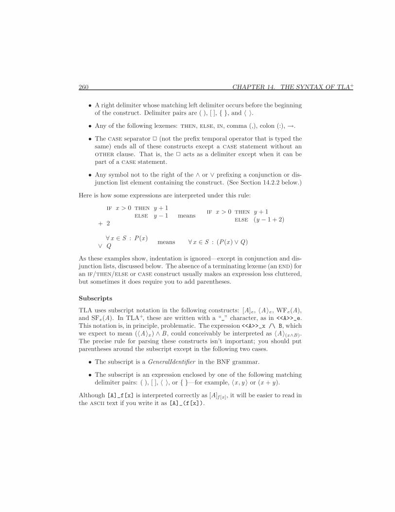
260 CHAPTER 14. THE SYNTAX OF TLA+
• A right delimiter whose matching left delimiter occurs before the beginningof the construct. Delimiter pairs are ( ), [ ], { }, and 〈 〉.• Any of the following lexemes: then, else, in, comma (,), colon (:), →.
• The case separator 2 (not the prefix temporal operator that is typed thesame) ends all of these constructs except a case statement without another clause. That is, the 2 acts as a delimiter except when it can bepart of a case statement.
• Any symbol not to the right of the ∧ or ∨ prefixing a conjunction or dis-junction list element containing the construct. (See Section 14.2.2 below.)
Here is how some expressions are interpreted under this rule:
if x > 0 then y + 1else y − 1
+ 2means if x > 0 then y + 1
else (y − 1 + 2)
∀ x ∈ S : P(x )∨ Q means ∀ x ∈ S : (P(x ) ∨Q)
As these examples show, indentation is ignored—except in conjunction and dis-junction lists, discussed below. The absence of a terminating lexeme (an end) foran if/then/else or case construct usually makes an expression less cluttered,but sometimes it does require you to add parentheses.
Subscripts
TLA uses subscript notation in the following constructs: [A]e , 〈A〉e , WFe(A),and SFe(A). In TLA+, these are written with a “_” character, as in <<A>>_e.This notation is, in principle, problematic. The expression <<A>>_x /\ B, whichwe expect to mean (〈A〉x ) ∧ B , could conceivably be interpreted as 〈A〉(x∧B).The precise rule for parsing these constructs isn’t important; you should putparentheses around the subscript except in the following two cases.
• The subscript is a GeneralIdentifier in the BNF grammar.
• The subscript is an expression enclosed by one of the following matchingdelimiter pairs: ( ), [ ], 〈 〉, or { }—for example, 〈x , y 〉 or (x + y).
Although [A]_f[x] is interpreted correctly as [A]f [x ], it will be easier to read inthe ascii text if you write it as [A]_(f[x]).
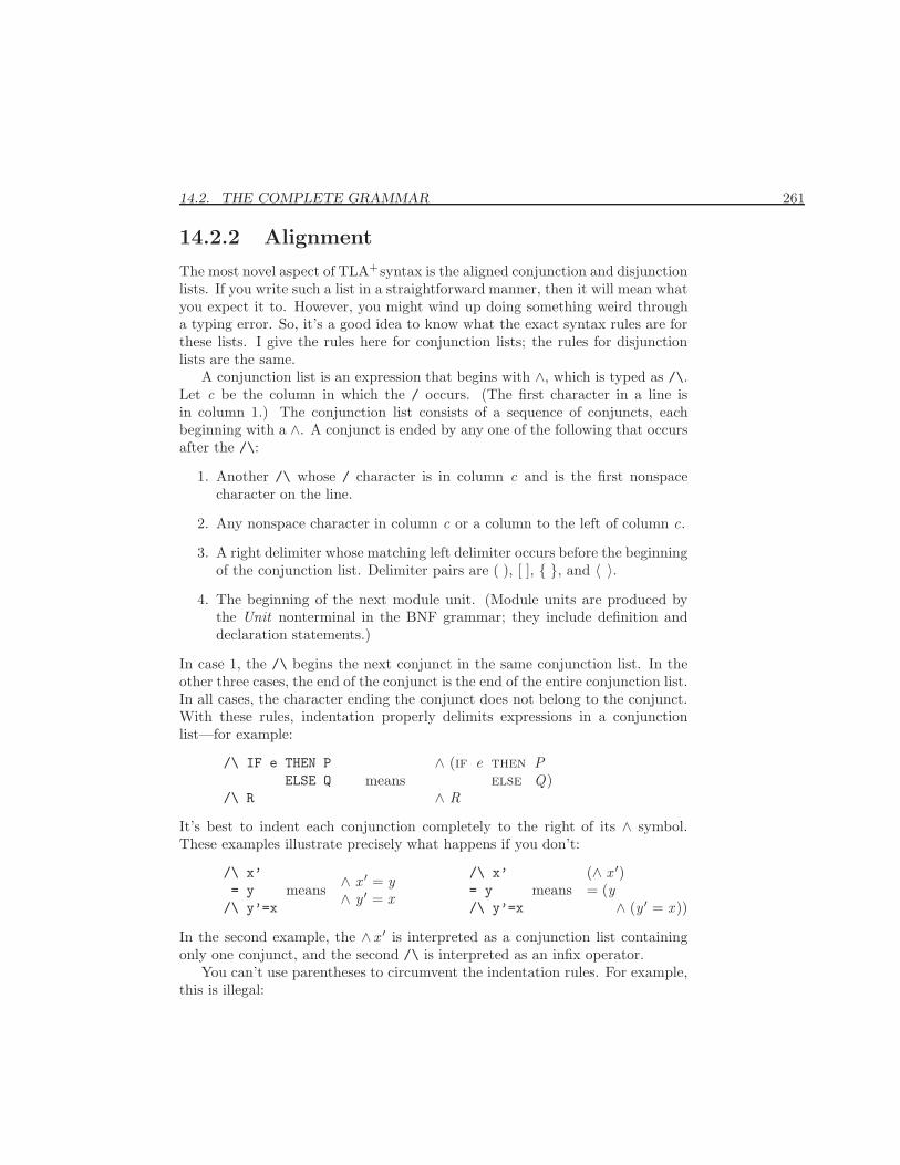
14.2. THE COMPLETE GRAMMAR 261
14.2.2 Alignment
The most novel aspect of TLA+ syntax is the aligned conjunction and disjunctionlists. If you write such a list in a straightforward manner, then it will mean whatyou expect it to. However, you might wind up doing something weird througha typing error. So, it’s a good idea to know what the exact syntax rules are forthese lists. I give the rules here for conjunction lists; the rules for disjunctionlists are the same.
A conjunction list is an expression that begins with ∧, which is typed as /\.Let c be the column in which the / occurs. (The first character in a line isin column 1.) The conjunction list consists of a sequence of conjuncts, eachbeginning with a ∧. A conjunct is ended by any one of the following that occursafter the /\:
1. Another /\ whose / character is in column c and is the first nonspacecharacter on the line.
2. Any nonspace character in column c or a column to the left of column c.
3. A right delimiter whose matching left delimiter occurs before the beginningof the conjunction list. Delimiter pairs are ( ), [ ], { }, and 〈 〉.
4. The beginning of the next module unit. (Module units are produced bythe Unit nonterminal in the BNF grammar; they include definition anddeclaration statements.)
In case 1, the /\ begins the next conjunct in the same conjunction list. In theother three cases, the end of the conjunct is the end of the entire conjunction list.In all cases, the character ending the conjunct does not belong to the conjunct.With these rules, indentation properly delimits expressions in a conjunctionlist—for example:
/\ IF e THEN PELSE Q
/\ Rmeans
∧ (if e then Pelse Q)
∧ R
It’s best to indent each conjunction completely to the right of its ∧ symbol.These examples illustrate precisely what happens if you don’t:
/\ x’= y
/\ y’=xmeans ∧ x ′ = y
∧ y ′ = x
/\ x’= y/\ y’=x
means(∧ x ′)= (y∧ (y ′ = x ))
In the second example, the ∧ x ′ is interpreted as a conjunction list containingonly one conjunct, and the second /\ is interpreted as an infix operator.
You can’t use parentheses to circumvent the indentation rules. For example,this is illegal:
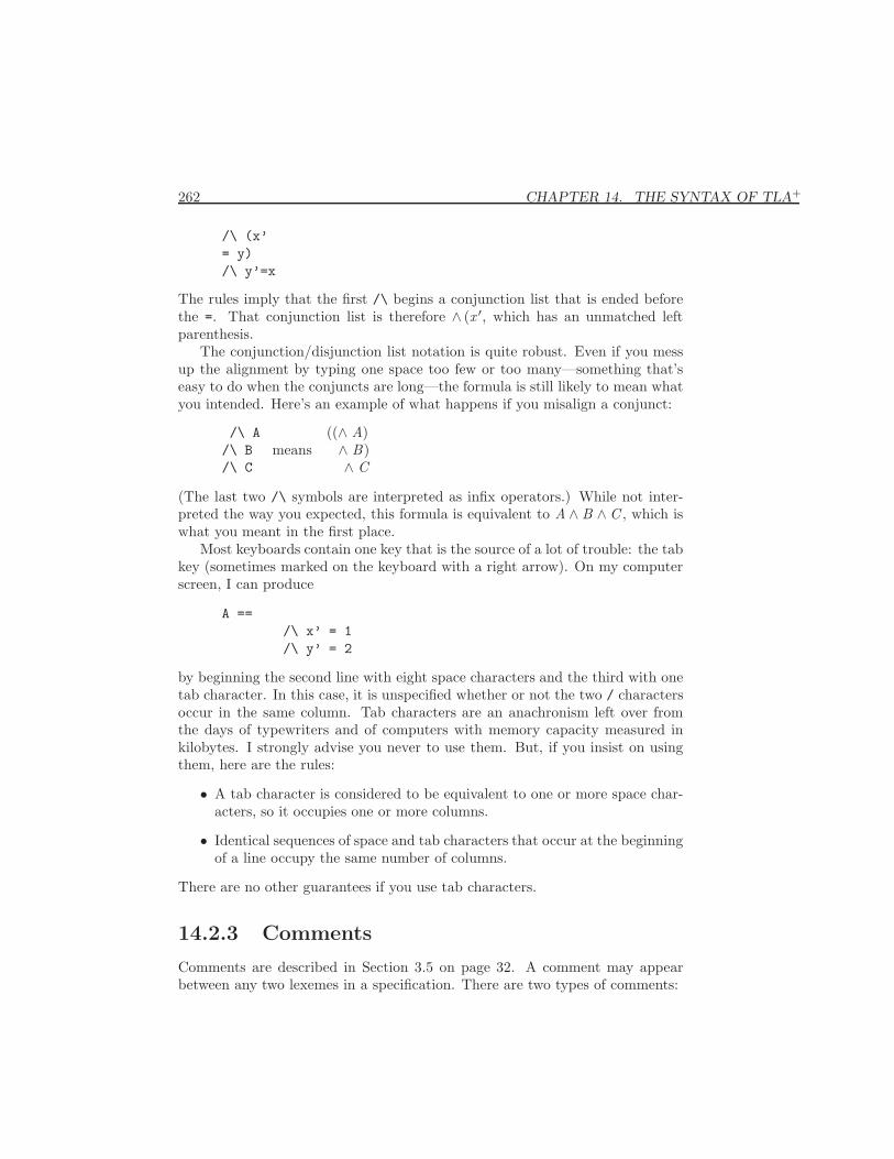
262 CHAPTER 14. THE SYNTAX OF TLA+
/\ (x’= y)/\ y’=x
The rules imply that the first /\ begins a conjunction list that is ended beforethe =. That conjunction list is therefore ∧ (x ′, which has an unmatched leftparenthesis.
The conjunction/disjunction list notation is quite robust. Even if you messup the alignment by typing one space too few or too many—something that’seasy to do when the conjuncts are long—the formula is still likely to mean whatyou intended. Here’s an example of what happens if you misalign a conjunct:
/\ A/\ B/\ C
means((∧ A)∧ B)∧ C
(The last two /\ symbols are interpreted as infix operators.) While not inter-preted the way you expected, this formula is equivalent to A ∧ B ∧ C , which iswhat you meant in the first place.
Most keyboards contain one key that is the source of a lot of trouble: the tabkey (sometimes marked on the keyboard with a right arrow). On my computerscreen, I can produce
A ==/\ x’ = 1/\ y’ = 2
by beginning the second line with eight space characters and the third with onetab character. In this case, it is unspecified whether or not the two / charactersoccur in the same column. Tab characters are an anachronism left over fromthe days of typewriters and of computers with memory capacity measured inkilobytes. I strongly advise you never to use them. But, if you insist on usingthem, here are the rules:
• A tab character is considered to be equivalent to one or more space char-acters, so it occupies one or more columns.
• Identical sequences of space and tab characters that occur at the beginningof a line occupy the same number of columns.
There are no other guarantees if you use tab characters.
14.2.3 Comments
Comments are described in Section 3.5 on page 32. A comment may appearbetween any two lexemes in a specification. There are two types of comments:
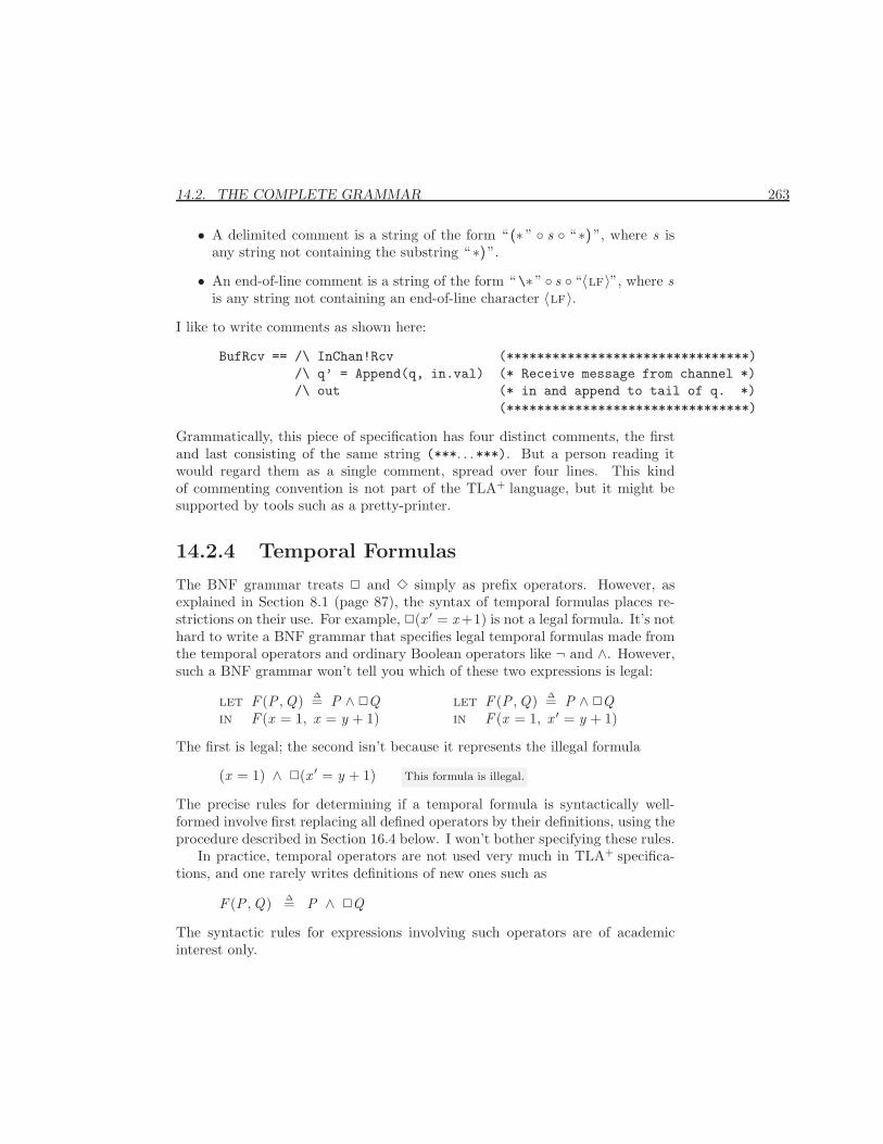
14.2. THE COMPLETE GRAMMAR 263
• A delimited comment is a string of the form “ (∗ ” ◦ s ◦ “ ∗) ”, where s isany string not containing the substring “ ∗) ”.
• An end-of-line comment is a string of the form “ \∗ ” ◦ s ◦ “〈lf〉”, where sis any string not containing an end-of-line character 〈lf〉.
I like to write comments as shown here:
BufRcv == /\ InChan!Rcv (********************************)/\ q’ = Append(q, in.val) (* Receive message from channel *)/\ out (* in and append to tail of q. *)
(********************************)
Grammatically, this piece of specification has four distinct comments, the firstand last consisting of the same string (***. . .***). But a person reading itwould regard them as a single comment, spread over four lines. This kindof commenting convention is not part of the TLA+ language, but it might besupported by tools such as a pretty-printer.
14.2.4 Temporal Formulas
The BNF grammar treats 2 and 3 simply as prefix operators. However, asexplained in Section 8.1 (page 87), the syntax of temporal formulas places re-strictions on their use. For example, 2(x ′ = x +1) is not a legal formula. It’s nothard to write a BNF grammar that specifies legal temporal formulas made fromthe temporal operators and ordinary Boolean operators like ¬ and ∧. However,such a BNF grammar won’t tell you which of these two expressions is legal:
let F (P ,Q) ∆= P ∧ 2Qin F (x = 1, x = y + 1)
let F (P ,Q) ∆= P ∧ 2Qin F (x = 1, x ′ = y + 1)
The first is legal; the second isn’t because it represents the illegal formula
(x = 1) ∧ 2(x ′ = y + 1) This formula is illegal.
The precise rules for determining if a temporal formula is syntactically well-formed involve first replacing all defined operators by their definitions, using theprocedure described in Section 16.4 below. I won’t bother specifying these rules.
In practice, temporal operators are not used very much in TLA+ specifica-tions, and one rarely writes definitions of new ones such as
F (P ,Q) ∆= P ∧ 2Q
The syntactic rules for expressions involving such operators are of academicinterest only.
264 CHAPTER 14. THE SYNTAX OF TLA+
14.2.5 Two Anomalies
There are two sources of ambiguity in the grammar of TLA+that you are unlikelyto encounter and that have ad hoc resolutions. The least unlikely of these arisesfrom the use of − as both an infix operator (as in 2 + 2) and a prefix operator(as in 2+−2). This poses no problem when − is used in an ordinary expression.However, there are two places in which an operator can appear by itself:
• As the argument of a higher-order operator, as in HOp(+, −).
• In an instance substitution, such as
instance M with Plus ← + , Minus ← −In both these cases, the symbol - is interpreted as the infix operator. You musttype -. to denote the prefix operator. You also have to type -. if you shouldever want to define the prefix − operator, as in:
−. a ∆= UMinus(a)
Remember that, in ordinary expressions, you just type - as usual for both op-erators.
The second source of ambiguity in the TLA+ syntax is an unlikely expressionof the form {x ∈ S : y ∈ T}, which might be taken to mean either of thefollowing:
let p ∆= y ∈ T in {x ∈ S : p}let p ∆= x ∈ S in {p : y ∈ T}
It is interpreted as the first formula.
14.3 What You Type
The grammar in Section 14.1.2 describes the ascii syntax for TLA+ specifica-tions. Typeset versions of specifications appear in this book. For example, thegrammar lists the infix operator \prec, but that operator is printed in specifi-cations as ≺. Figure 13.16 on page 243 gives the correspondence between theascii and typeset versions of all TLA+ symbols for which the correspondencemay not be obvious.
Finally, Figure 13.13 on page 240 lists all the user-definable infix, postfix,and prefix operator symbols of TLA+. It also indicates which of them are definedby the standard modules. This is a good place to look when choosing notationfor your specification.
Chapter 15
The Operators of TLA+
This chapter describes the built-in operators of TLA+. Most of these opera-tors have been described in Part I. Here, you can find brief explanations ofthe operators, along with references to the longer descriptions in Part I. Theexplanations cover some subtle points that are not mentioned elsewhere. Thechapter can serve as a reference manual for readers who have finished Part I orwho are already familiar enough with the mathematical concepts that the briefexplanations are all they need.
The chapter includes a formal semantics of the operators. The rigorousdescription of TLA+ that a formal semantics provides is usually needed only bypeople building TLA+ tools. If you’re not building a tool and don’t have a specialfondness for formalism, you will probably want to skip all the subsections titledFormal Semantics. However, you may some day encounter an obscure questionabout the meaning of a TLA+ operator that is answered only by the formalsemantics.
This chapter also defines some of the “semantic” conditions on the syntaxof TLA+ that are omitted from the grammar of Chapter 14. For example, ittells you that [a : Nat , a : boolean] is an illegal expression. Other semanticconditions on expressions arise from a combination of the definitions in thischapter and the conditions stated in Chapter 16. For example, this chapterdefines ∃ x , x : p to equal ∃ x : (∃ x : p), and Chapter 16 tells you that the latterexpression is illegal.
15.1 Constant Operators
We first define the constant operators of TLA+. These are the operators ofordinary mathematics, having nothing to do with TLA or temporal logic. Allthe constant operators of TLA+ are listed in Figure 13.9 on page 238 and Fig-
265
266 CHAPTER 15. THE OPERATORS OF TLA+
ure 13.10 on page 239.An operator combines one or more expressions into a “larger” expression.
For example, the set union operator ∪ combines two expressions e1 and e2 intothe expression e1 ∪ e2. Some operators don’t have such simple names as ∪. Forexample, there’s no simple name for the operator that combines the n expressionse1, . . . , en to form the expression {e1, . . . , en}. We could name it { , . . . , } or{ , . . . , }, but that would be awkward. Instead of explicitly mentioning theoperator, I’ll refer to the construct {e1, . . . , en}. The distinction between anoperator like ∪ and the nameless one used in the construct {e1, . . . , en} is purelysyntactic, with no mathematical significance. In Chapter 16, I will abstract awayfrom this syntactic difference and treat all operators uniformly. For now, I’ll staycloser to the syntax.
Formal Semantics
A formal semantics for a language is a translation from that language into someform of mathematics. We assign a mathematical expression [[e]], called the mean-ing of e, to certain terms e in the language. Since we presumably understandthe mathematics, we know what [[e]] means, and that tells us what e means.
Meaning is generally defined inductively. For example, the meaning [[e1∪e2]]of the expression e1 ∪ e2 would be defined in terms of the meanings [[e1]] and[[e2]] of its subexpressions. This definition is said to define the semantics of theoperator ∪.
Because much of TLA+ is a language for expressing ordinary mathematics,much of its semantics is trivial. For example, the semantics of ∪ can be defined by
[[e1 ∪ e2]]∆= [[e1]] ∪ [[e2]]
In this definition, the ∪ to the left of the ∆= is the TLA+ symbol, while the oneto the right is the set-union operator of ordinary mathematics. I could make thedistinction between the two uses of the symbol ∪ more obvious by writing
[[e1 \cup e2]]∆= [[e1]] ∪ [[e2]]
But, that wouldn’t make the definition any less trivial.Instead of trying to maintain a distinction between the TLA+ operator ∪
and the operator of set theory that’s written the same, I simply use TLA+ asthe language of mathematics in which to define the semantics of TLA+. Thatis, I take as primitive certain TLA+ operators that, like ∪, correspond to well-known mathematical operators. I describe the formal semantics of the constantoperators of TLA+ by defining them in terms of these primitive operators. I alsodescribe the semantics of some of the primitive operators by stating the axiomsthat they satisfy.
15.1. CONSTANT OPERATORS 267
15.1.1 Boolean Operators
The truth values of logic are written in TLA+ as true and false. The built-inconstant boolean is the set consisting of those two values:
boolean∆= {true, false}
TLA+ provides the usual operators of propositional logic:
∧ ∨ ¬ ⇒ (implication) ≡ true false
They are explained in Section 1.1. Conjunctions and disjunctions can be writtenas aligned lists:
∧ p1
...∧ pn
∆= p1 ∧ . . . ∧ pn
∨ p1
...∨ pn
∆= p1 ∨ . . . ∨ pn
The standard quantified formulas of predicate logic are written in TLA+ as:
∀ x : P ∃ x : P
I call these the unbounded quantifier constructions. The bounded versions arewritten as:
∀ x ∈ S : p ∃ x ∈ S : p
The meanings of these expressions are described in Section 1.3. TLA+ allowssome common abbreviations—for example:
∀ x , y : p ∆= ∀ x : (∀ y : p)
∃ x , y ∈ S , z ∈ T : p ∆= ∃ x ∈ S : (∃ y ∈ S : (∃ z ∈ T : p))
TLA+ also allows bounded quantification over tuples, such as
∀ 〈x , y 〉 ∈ S : p
This formula is true iff, for any pair 〈a, b 〉 in S , the formula obtained from p bysubstituting a for x and b for y is true.
Formal Semantics
Propositional and predicate logic, along with set theory, form the foundationof ordinary mathematics. In defining the semantics of TLA+, we therefore takeas primitives the operators of propositional logic and the simple unboundedquantifier constructs ∃ x : p and ∀ x : p, where x is an identifier. Among theBoolean operators described above, this leaves only the general forms of thequantifiers, given by the BNF grammar of Chapter 14, whose meanings must
268 CHAPTER 15. THE OPERATORS OF TLA+
be defined. This is done by defining those general forms in terms of the simpleforms.
The unbounded operators have the general forms:
∀ x 1, . . . , xn : p ∃ x 1, . . . , xn : p
where each x i is an identifier. They are defined in terms of quantification overa single variable by:
∀ x 1, . . . , xn : p ∆= ∀ x 1 : (∀ x 2 : (. . . ∀ xn : p) . . .)
and similarly for ∃ . The bounded operators have the general forms:
∀y1 ∈ S 1, . . . ,yn ∈ Sn : p ∃y1 ∈ S 1, . . . ,yn ∈ Sn : p
where each yi has the form x 1, . . . , x k or 〈x 1, . . . , x k 〉, and each x j is an identi-fier. The general forms of ∀ are defined inductively by
∀ x 1, . . . , x k ∈ S : p ∆= ∀ x 1, . . . , x k : (x 1 ∈ S ) ∧ . . . ∧ (x k ∈ S )⇒ p
∀y1 ∈ S 1, . . . , yn ∈ Sn : p ∆= ∀y1 ∈ S 1 : . . . ∀ : yn ∈ Sn : p
∀ 〈x 1, . . . , x k 〉 ∈ S : p ∆= ∀ x 1, . . . , x k : (〈x 1, . . . , x k 〉 ∈ S )⇒ p
where the yi are as before. In these expressions, S and the S i lie outside thescope of the quantifier’s bound identifiers. The definitions for ∃ are similar. Inparticular:
∃ 〈x 1, . . . , x k 〉 ∈ S : p ∆= ∃ x 1, . . . , x k : (〈x 1, . . . , x k 〉 ∈ S ) ∧ p
See Section 15.1.9 for further details about tuples.
15.1.2 The Choose Operator
A simple unbounded choose expression has the form
choose x : p
As explained in Section 6.6, the value of this expression is some arbitrary valuev such that p is true if v is substituted for x , if such a v exists. If no such vexists, then the expression has a completely arbitrary value.
The bounded form of the choose expression is:
choose x ∈ S : p
It is defined in terms of the unbounded form by
choose x ∈ S : p ∆= choose x : (x ∈ S ) ∧ p(15.1)
15.1. CONSTANT OPERATORS 269
It is equal to some arbitrary value v in S such that p, with v substituted forx , is true—if such a v exists. If no such v exists, the choose expression has acompletely arbitrary value.
A choose expression can also be used to choose a tuple. For example
choose 〈x , y 〉 ∈ S : p
equals some pair 〈v ,w 〉 in S such that p, with v substituted for x and w sub-stituted for y, is true—if such a pair exists. If no such pair exists, it has anarbitrary value, which need not be a pair.
The unbounded choose operator satisfies the following two rules:
(∃ x : P(x )) ≡ P(choose x : P(x ))(∀ x : P(x ) = Q(x ))⇒ ((choose x : P(x )) = choose x : Q(x ))
(15.2)
for any operators P and Q . We know nothing about the value chosen by chooseexcept what we can deduce from these rules.
The second rule allows us to deduce the equality of certain choose expres-sions that we might expect to be different. In particular, for any operator P , ifthere exists no x satisfying P(x ), then choose x : P(x ) equals the unique valuechoose x : false. For example, the Reals module defines division by
a/b ∆= choose c ∈ Real : a = b ∗ c
For any nonzero number a, there exists no number c such that a = 0∗ c. Hence,a/0 equals choose c : false, for any nonzero a. We can therefore deduce that1/0 equals 2/0.
We would expect to be unable to deduce anything about the nonsensicalexpression 1/0. It’s a bit disquieting to prove that it equals 2/0. If this upsetsyou, here’s a way to define division that will make you happier. First define anoperator Choice so that Choice(v , P) equals choose x : P(x ) if there exists anx satisfying P(x ), and otherwise equals some arbitrary value that depends onv . There are many ways to define Choice; here’s one:
Choice(v , P( )) ∆= if ∃ x : P(x ) then choose x : P(x )else (choose x : x .a = v).b
You can then define division by
a/b ∆= let P(c) ∆= (c ∈ Real) ∧ (a = b ∗ c)in Choice(a, P)
This definition makes it impossible to deduce any relation between 1/0 and 2/0.You can use Choice instead of choose whenever this kind of problem arises—ifyou consider 1/0 equaling 2/0 to be a problem. But there is seldom any practicalreason for worrying about it.
270 CHAPTER 15. THE OPERATORS OF TLA+
Formal Semantics
We take the construct choose x : p, where x is an identifier, to be primitive.This form of the choose operator is known to mathematicians as Hilbert’s ε. Itsmeaning is defined mathematically by the rules (15.2). Leisenring [3] presents adetailed mathematical exposition of Hilbert’s ε.
An unbounded choose of a tuple is defined in terms of the simple unboundedchoose construct by
choose 〈x 1, . . . , xn 〉 : p ∆= choose y : (∃ x 1, . . . , xn : (y = 〈x 1, . . . , xn 〉) ∧ p)
where y is an identifier that is different from the x i and does not occur in p.The bounded choose construct is defined in terms of unbounded choose by(15.1), where x can be either an identifier or a tuple.
15.1.3 The Three Interpretations of Boolean Operators
The meaning of a Boolean operator when applied to Boolean values is a standardpart of traditional mathematics. Everyone agrees that true ∧ false equalsfalse. However, because TLA+ is untyped, an expression like 2 ∧ 〈5〉 is legal.We must therefore decide what it means. There are three ways of doing this,which I call the conservative, moderate, and liberal interpretations.
In the conservative interpretation, the value of an expression like 2 ∧ 〈5〉 iscompletely unspecified. It could equal
√2. It need not equal 〈5〉 ∧ 2. Hence,
the ordinary laws of logic, such as the commutativity of ∧, are valid only forBoolean values.
In the liberal interpretation, the value of 2 ∧ 〈5〉 is specified to be a Boolean.It is not specified whether it equals true or false. However, all the ordinarylaws of logic, such as the commutativity of ∧, are valid. Hence, 2 ∧ 〈5〉 equals〈5〉 ∧ 2. More precisely, any tautology of propositional or predicate logic, suchas
(∀ x : p) ≡ ¬(∃ x : ¬p)
is valid, even if p is not necessarily a Boolean for all values of x .1 It is easyto show that the liberal approach is sound.2 For example, one way of definingoperators that satisfy the liberal interpretation is to consider any nonBooleanvalue to be equivalent to false.
The conservative and liberal interpretations are equivalent for most speci-fications, except for ones that use Boolean-valued functions. In practice, the
1Equality (=) is not an operator of propositional or predicate logic; this tautology need notbe valid for nonBoolean values if ≡ is replaced by =.
2A sound logic in one in which false is not provable.
15.1. CONSTANT OPERATORS 271
conservative interpretation doesn’t permit you to use f [x ] as a Boolean expres-sion even if f is defined to be a Boolean-valued function. For example, supposewe define the function tnat by
tnat ∆= [n ∈ Nat 7→ true]
so tnat [n] equals true for all n in Nat . The formula
∀n ∈ Nat : tnat [n](15.3)
equals true in the liberal interpretation, but not in the conservative interpre-tation. Formula (15.3) is equivalent to
∀n : (n ∈ Nat)⇒ tnat [n]
which asserts that (n ∈ Nat)⇒ tnat [n] is true for all n, including, for example,n = 1/2. For (15.3) to equal true, the formula (1/2 ∈ Nat) ⇒ tnat [1/2],which equals false⇒ tnat [1/2], must equal true. But the value of tnat [1/2] isnot specified; it might equal
√2. The formula false⇒ √2 equals true in the
liberal interpretation; its value is unspecified in the conservative interpretation.Hence, the value of (15.3) is unspecified in the conservative interpretation. If weare using the conservative interpretation, instead of (15.3), we should write
∀n ∈ Nat : (tnat [n] = true)
This formula equals true in both interpretations.The conservative interpretation is philosophically more satisfying, since it
makes no assumptions about a silly expression like 2 ∧ 〈5〉. However, as wehave just seen, it would be nice if the not-so-silly formula false⇒ √2 equaledtrue. We therefore introduce the moderate interpretation, which lies betweenthe conservative and liberal interpretations. It assumes only that expressionsinvolving false and true have their expected values—for example, false⇒ √2equals true, and false ∧ 2 equals false. In the moderate interpretation, (15.3)equals true, but the value of 〈5〉 ∧ 2 is still completely unspecified.
The laws of logic still do not hold unconditionally in the moderate interpre-tation. The formulas p ∧ q and q ∧ p are equivalent only if p and q are bothBooleans, or if one of them equals false. When using the moderate interpre-tation, we still have to check that all the relevant values are Booleans beforeapplying any of the ordinary rules of logic in a proof. This can be burdensomein practice.
The semantics of TLA+ asserts that the rules of the moderate interpreta-tion are valid. The liberal interpretation is neither required nor forbidden. Youshould write specifications that make sense under the moderate interpretation.However, you (and the implementer of a tool) are free to use the liberal inter-pretation if you wish.
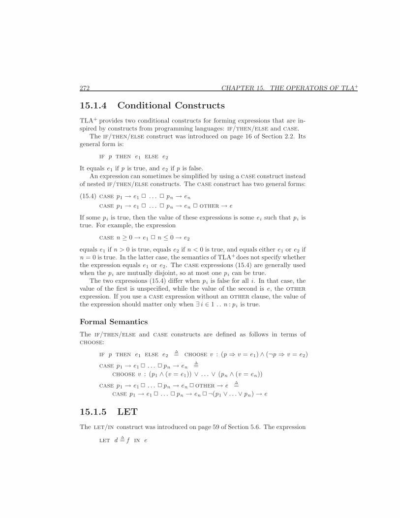
272 CHAPTER 15. THE OPERATORS OF TLA+
15.1.4 Conditional Constructs
TLA+ provides two conditional constructs for forming expressions that are in-spired by constructs from programming languages: if/then/else and case.
The if/then/else construct was introduced on page 16 of Section 2.2. Itsgeneral form is:
if p then e1 else e2
It equals e1 if p is true, and e2 if p is false.An expression can sometimes be simplified by using a case construct instead
of nested if/then/else constructs. The case construct has two general forms:
case p1 → e1 2 . . . 2 pn → en
case p1 → e1 2 . . . 2 pn → en 2 other→ e(15.4)
If some pi is true, then the value of these expressions is some ei such that pi istrue. For example, the expression
case n ≥ 0→ e1 2 n ≤ 0→ e2
equals e1 if n > 0 is true, equals e2 if n < 0 is true, and equals either e1 or e2 ifn = 0 is true. In the latter case, the semantics of TLA+does not specify whetherthe expression equals e1 or e2. The case expressions (15.4) are generally usedwhen the pi are mutually disjoint, so at most one pi can be true.
The two expressions (15.4) differ when pi is false for all i . In that case, thevalue of the first is unspecified, while the value of the second is e, the otherexpression. If you use a case expression without an other clause, the value ofthe expression should matter only when ∃ i ∈ 1 . . n : pi is true.
Formal Semantics
The if/then/else and case constructs are defined as follows in terms ofchoose:
if p then e1 else e2∆= choose v : (p ⇒ v = e1) ∧ (¬p ⇒ v = e2)
case p1 → e1 2 . . . 2 pn → en∆=
choose v : (p1 ∧ (v = e1)) ∨ . . . ∨ (pn ∧ (v = en))
case p1 → e1 2 . . . 2 pn → en 2other→ e ∆=case p1 → e1 2 . . . 2 pn → en 2¬(p1 ∨ . . . ∨ pn)→ e
15.1.5 LET
The let/in construct was introduced on page 59 of Section 5.6. The expression
let d ∆= f in e
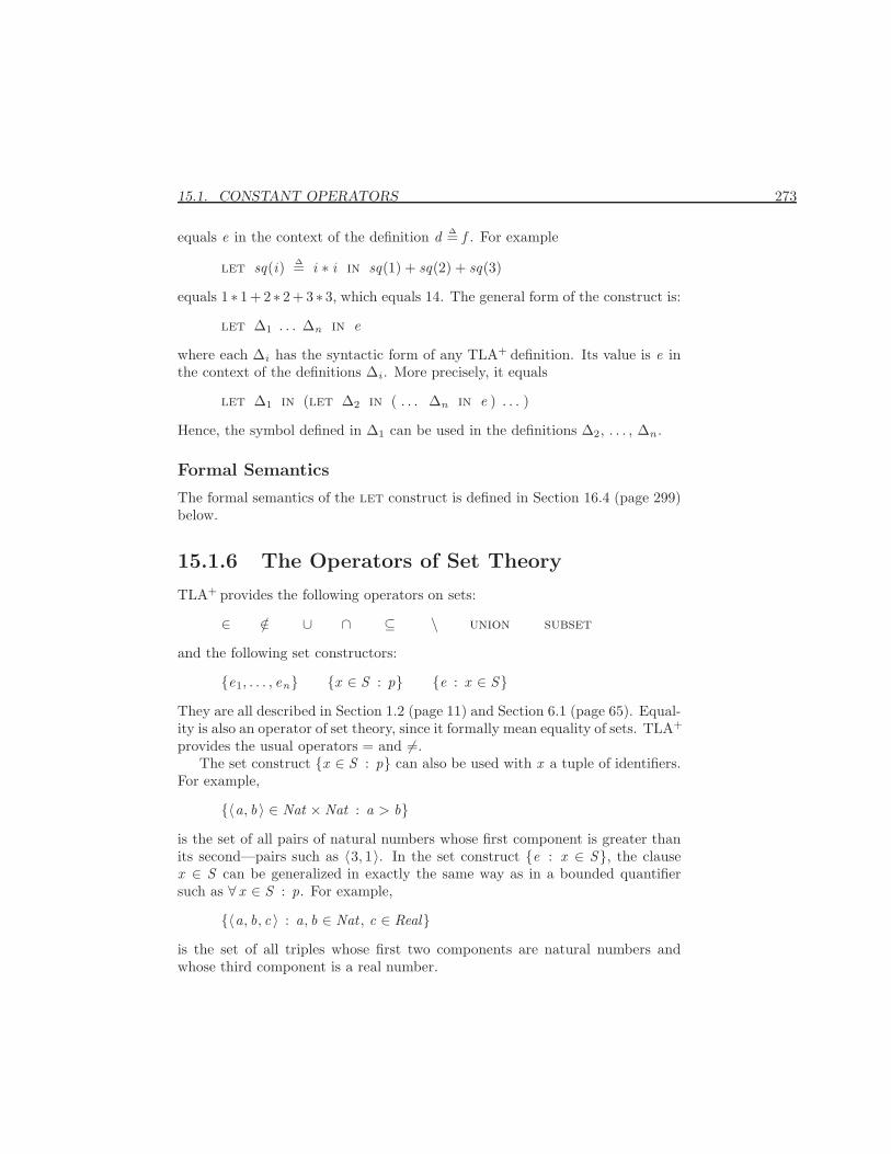
15.1. CONSTANT OPERATORS 273
equals e in the context of the definition d ∆= f . For example
let sq(i) ∆= i ∗ i in sq(1) + sq(2) + sq(3)
equals 1 ∗ 1+2 ∗ 2+3 ∗ 3, which equals 14. The general form of the construct is:
let ∆1 . . . ∆n in e
where each ∆i has the syntactic form of any TLA+ definition. Its value is e inthe context of the definitions ∆i . More precisely, it equals
let ∆1 in (let ∆2 in ( . . . ∆n in e ) . . . )
Hence, the symbol defined in ∆1 can be used in the definitions ∆2, . . . , ∆n .
Formal Semantics
The formal semantics of the let construct is defined in Section 16.4 (page 299)below.
15.1.6 The Operators of Set Theory
TLA+ provides the following operators on sets:
∈ /∈ ∪ ∩ ⊆ \ union subset
and the following set constructors:
{e1, . . . , en} {x ∈ S : p} {e : x ∈ S}They are all described in Section 1.2 (page 11) and Section 6.1 (page 65). Equal-ity is also an operator of set theory, since it formally mean equality of sets. TLA+
provides the usual operators = and 6=.The set construct {x ∈ S : p} can also be used with x a tuple of identifiers.
For example,
{〈a, b 〉 ∈ Nat ×Nat : a > b}is the set of all pairs of natural numbers whose first component is greater thanits second—pairs such as 〈3, 1〉. In the set construct {e : x ∈ S}, the clausex ∈ S can be generalized in exactly the same way as in a bounded quantifiersuch as ∀ x ∈ S : p. For example,
{〈a, b, c 〉 : a, b ∈ Nat , c ∈ Real}is the set of all triples whose first two components are natural numbers andwhose third component is a real number.
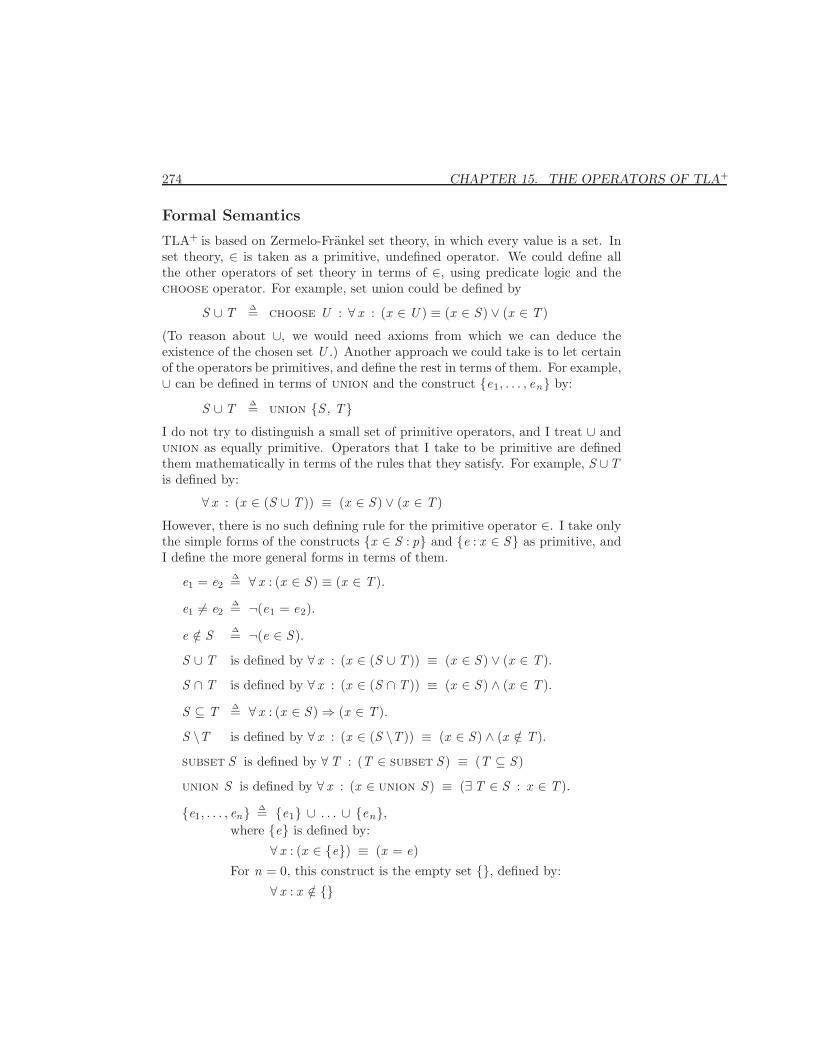
274 CHAPTER 15. THE OPERATORS OF TLA+
Formal Semantics
TLA+ is based on Zermelo-Frankel set theory, in which every value is a set. Inset theory, ∈ is taken as a primitive, undefined operator. We could define allthe other operators of set theory in terms of ∈, using predicate logic and thechoose operator. For example, set union could be defined by
S ∪ T ∆= choose U : ∀ x : (x ∈ U ) ≡ (x ∈ S ) ∨ (x ∈ T )
(To reason about ∪, we would need axioms from which we can deduce theexistence of the chosen set U .) Another approach we could take is to let certainof the operators be primitives, and define the rest in terms of them. For example,∪ can be defined in terms of union and the construct {e1, . . . , en} by:
S ∪ T ∆= union {S , T}I do not try to distinguish a small set of primitive operators, and I treat ∪ andunion as equally primitive. Operators that I take to be primitive are definedthem mathematically in terms of the rules that they satisfy. For example, S ∪Tis defined by:
∀ x : (x ∈ (S ∪ T )) ≡ (x ∈ S ) ∨ (x ∈ T )
However, there is no such defining rule for the primitive operator ∈. I take onlythe simple forms of the constructs {x ∈ S : p} and {e : x ∈ S} as primitive, andI define the more general forms in terms of them.
e1 = e2∆= ∀ x : (x ∈ S ) ≡ (x ∈ T ).
e1 6= e2∆= ¬(e1 = e2).
e /∈ S ∆= ¬(e ∈ S ).
S ∪ T is defined by ∀ x : (x ∈ (S ∪ T )) ≡ (x ∈ S ) ∨ (x ∈ T ).
S ∩ T is defined by ∀ x : (x ∈ (S ∩ T )) ≡ (x ∈ S ) ∧ (x ∈ T ).
S ⊆ T ∆= ∀ x : (x ∈ S )⇒ (x ∈ T ).
S \T is defined by ∀ x : (x ∈ (S \T )) ≡ (x ∈ S ) ∧ (x /∈ T ).
subset S is defined by ∀T : (T ∈ subset S ) ≡ (T ⊆ S )
union S is defined by ∀ x : (x ∈ union S ) ≡ (∃T ∈ S : x ∈ T ).
{e1, . . . , en} ∆= {e1} ∪ . . . ∪ {en},where {e} is defined by:
∀ x : (x ∈ {e}) ≡ (x = e)
For n = 0, this construct is the empty set {}, defined by:
∀ x : x /∈ {}
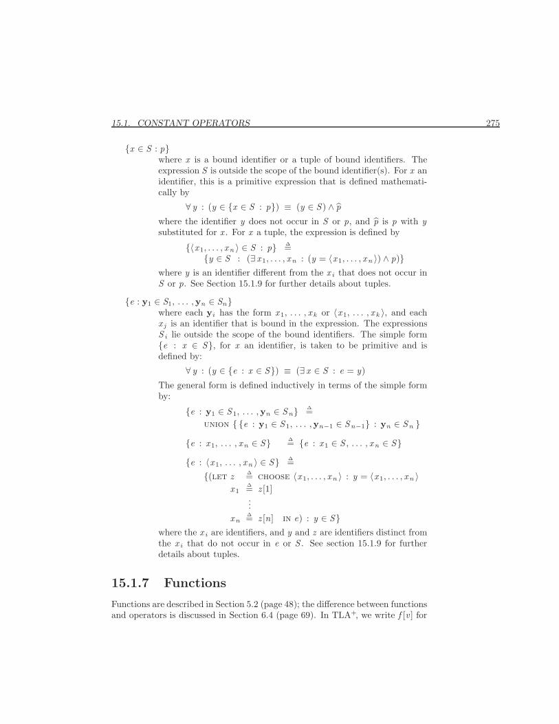
15.1. CONSTANT OPERATORS 275
{x ∈ S : p}where x is a bound identifier or a tuple of bound identifiers. Theexpression S is outside the scope of the bound identifier(s). For x anidentifier, this is a primitive expression that is defined mathemati-cally by
∀ y : (y ∈ {x ∈ S : p}) ≡ (y ∈ S ) ∧ p
where the identifier y does not occur in S or p, and p is p with ysubstituted for x . For x a tuple, the expression is defined by
{〈x 1, . . . , xn 〉 ∈ S : p} ∆={y ∈ S : (∃ x 1, . . . , xn : (y = 〈x 1, . . . , xn 〉) ∧ p)}
where y is an identifier different from the x i that does not occur inS or p. See Section 15.1.9 for further details about tuples.
{e : y1 ∈ S1, . . . ,yn ∈ Sn}where each yi has the form x 1, . . . , x k or 〈x 1, . . . , x k 〉, and eachx j is an identifier that is bound in the expression. The expressionsS i lie outside the scope of the bound identifiers. The simple form{e : x ∈ S}, for x an identifier, is taken to be primitive and isdefined by:
∀ y : (y ∈ {e : x ∈ S}) ≡ (∃ x ∈ S : e = y)
The general form is defined inductively in terms of the simple formby:
{e : y1 ∈ S 1, . . . ,yn ∈ Sn} ∆=union { {e : y1 ∈ S 1, . . . ,yn−1 ∈ Sn−1} : yn ∈ Sn }
{e : x 1, . . . , xn ∈ S} ∆= {e : x 1 ∈ S , . . . , xn ∈ S}{e : 〈x 1, . . . , xn 〉 ∈ S} ∆=
{(let z ∆= choose 〈x 1, . . . , xn 〉 : y = 〈x 1, . . . , xn 〉x 1
∆= z [1]...
xn∆= z [n] in e) : y ∈ S}
where the x i are identifiers, and y and z are identifiers distinct fromthe x i that do not occur in e or S . See section 15.1.9 for furtherdetails about tuples.
15.1.7 Functions
Functions are described in Section 5.2 (page 48); the difference between functionsand operators is discussed in Section 6.4 (page 69). In TLA+, we write f [v ] for
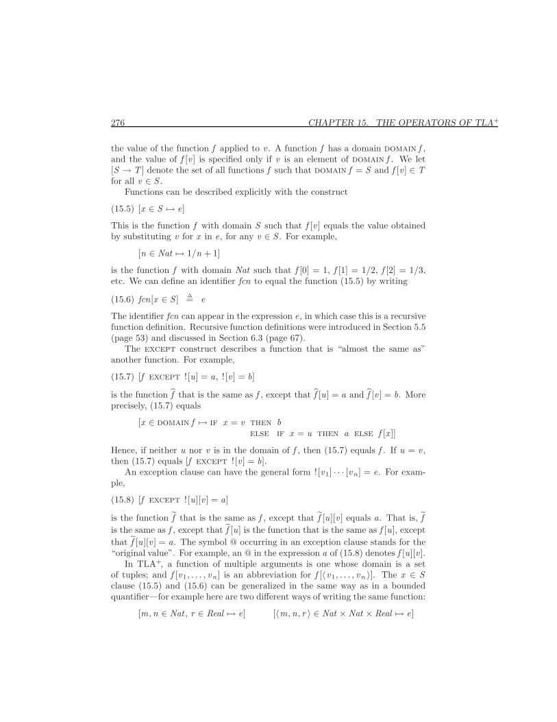
276 CHAPTER 15. THE OPERATORS OF TLA+
the value of the function f applied to v . A function f has a domain domain f ,and the value of f [v ] is specified only if v is an element of domain f . We let[S → T ] denote the set of all functions f such that domain f = S and f [v ] ∈ Tfor all v ∈ S .
Functions can be described explicitly with the construct
[x ∈ S 7→ e](15.5)
This is the function f with domain S such that f [v ] equals the value obtainedby substituting v for x in e, for any v ∈ S . For example,
[n ∈ Nat 7→ 1/n + 1]
is the function f with domain Nat such that f [0] = 1, f [1] = 1/2, f [2] = 1/3,etc. We can define an identifier fcn to equal the function (15.5) by writing
fcn[x ∈ S ] ∆= e(15.6)
The identifier fcn can appear in the expression e, in which case this is a recursivefunction definition. Recursive function definitions were introduced in Section 5.5(page 53) and discussed in Section 6.3 (page 67).
The except construct describes a function that is “almost the same as”another function. For example,
[f except ! [u] = a, ! [v ] = b](15.7)
is the function f that is the same as f , except that f [u] = a and f [v ] = b. Moreprecisely, (15.7) equals
[x ∈ domain f 7→ if x = v then belse if x = u then a else f [x ]]
Hence, if neither u nor v is in the domain of f , then (15.7) equals f . If u = v ,then (15.7) equals [f except ! [v ] = b].
An exception clause can have the general form ![v1] · · · [vn ] = e. For exam-ple,
[f except ! [u][v ] = a](15.8)
is the function f that is the same as f , except that f [u][v ] equals a. That is, fis the same as f , except that f [u] is the function that is the same as f [u], exceptthat f [u][v ] = a. The symbol @ occurring in an exception clause stands for the“original value”. For example, an @ in the expression a of (15.8) denotes f [u][v ].
In TLA+, a function of multiple arguments is one whose domain is a setof tuples; and f [v1, . . . , vn ] is an abbreviation for f [〈v1, . . . , vn 〉]. The x ∈ Sclause (15.5) and (15.6) can be generalized in the same way as in a boundedquantifier—for example here are two different ways of writing the same function:
[m,n ∈ Nat , r ∈ Real 7→ e] [〈m,n, r 〉 ∈ Nat ×Nat × Real 7→ e]
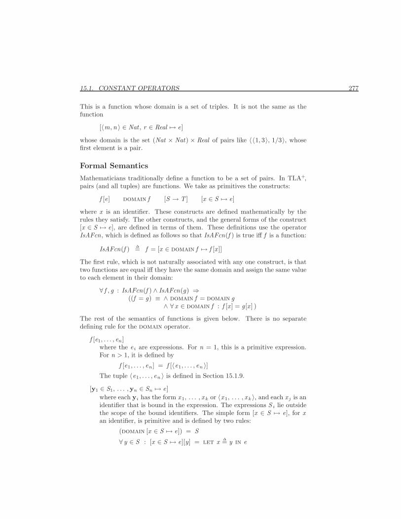
15.1. CONSTANT OPERATORS 277
This is a function whose domain is a set of triples. It is not the same as thefunction
[〈m,n 〉 ∈ Nat , r ∈ Real 7→ e]
whose domain is the set (Nat × Nat) × Real of pairs like 〈〈1, 3〉, 1/3〉, whosefirst element is a pair.
Formal Semantics
Mathematicians traditionally define a function to be a set of pairs. In TLA+,pairs (and all tuples) are functions. We take as primitives the constructs:
f [e] domain f [S → T ] [x ∈ S 7→ e]
where x is an identifier. These constructs are defined mathematically by therules they satisfy. The other constructs, and the general forms of the construct[x ∈ S 7→ e], are defined in terms of them. These definitions use the operatorIsAFcn, which is defined as follows so that IsAFcn(f ) is true iff f is a function:
IsAFcn(f ) ∆= f = [x ∈ domain f 7→ f [x ]]
The first rule, which is not naturally associated with any one construct, is thattwo functions are equal iff they have the same domain and assign the same valueto each element in their domain:
∀ f , g : IsAFcn(f ) ∧ IsAFcn(g) ⇒((f = g) ≡ ∧ domain f = domain g
∧ ∀ x ∈ domain f : f [x ] = g[x ] )
The rest of the semantics of functions is given below. There is no separatedefining rule for the domain operator.
f [e1, . . . , en ]where the ei are expressions. For n = 1, this is a primitive expression.For n > 1, it is defined by
f [e1, . . . , en ] = f [〈e1, . . . , en 〉]The tuple 〈e1, . . . , en 〉 is defined in Section 15.1.9.
[y1 ∈ S1, . . . ,yn ∈ Sn 7→ e]where each yi has the form x 1, . . . , x k or 〈x 1, . . . , x k 〉, and each x j is anidentifier that is bound in the expression. The expressions S i lie outsidethe scope of the bound identifiers. The simple form [x ∈ S 7→ e], for xan identifier, is primitive and is defined by two rules:
(domain [x ∈ S 7→ e]) = S
∀ y ∈ S : [x ∈ S 7→ e][y] = let x ∆= y in e
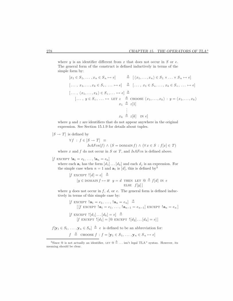
278 CHAPTER 15. THE OPERATORS OF TLA+
where y is an identifier different from x that does not occur in S or e.The general form of the construct is defined inductively in terms of thesimple form by:
[x 1 ∈ S 1, . . . , xn ∈ Sn 7→ e] ∆= [ 〈x 1, . . . , xn 〉 ∈ S 1 × . . .× Sn 7→ e]
[ . . . , x 1, . . . , x k ∈ S i , . . . 7→ e] ∆= [ . . . , x 1 ∈ S i , . . . , x k ∈ S i , . . . 7→ e]
[ . . . , 〈x 1, . . . , x k 〉 ∈ S i , . . . 7→ e] ∆=
[ . . . , y ∈ S i , . . . 7→ let z ∆= choose 〈x 1, . . . , x k 〉 : y = 〈x 1, . . . , x k 〉x 1
∆= z [1]...
x k∆= z [k ] in e]
where y and z are identifiers that do not appear anywhere in the originalexpression. See Section 15.1.9 for details about tuples.
[S → T ] is defined by
∀ f : f ∈ [S → T ] ≡IsAFcn(f ) ∧ (S = domain f ) ∧ (∀ x ∈ S : f [x ] ∈ T )
where x and f do not occur in S or T , and IsAFcn is defined above.
[f except !a1 = e1, . . . , !an = en ]where each ai has the form [d1] . . . [dk ] and each d j is an expression. Forthe simple case when n = 1 and a1 is [d ], this is defined by3
[f except ! [d ] = e] ∆=[y ∈ domain f 7→ if y = d then let @ ∆= f [d ] in e
else f [y] ]
where y does not occur in f , d , or e. The general form is defined induc-tively in terms of this simple case by:
[f except !a1 = e1, . . . , !an = en ] ∆=[ [f except !a1 = e1, . . . , !an−1 = en−1] except !an = en ]
[f except ! [d1] . . . [dk ] = e] ∆=[f except ! [d1] = [@ except ! [d2] . . . [dk ] = e] ]
f [y1 ∈ S1, . . . ,yn ∈ Sn ] ∆= e is defined to be an abbreviation for:
f ∆= choose f : f = [y1 ∈ S 1, . . . ,yn ∈ Sn 7→ e]
3Since @ is not actually an identifier, let @∆= . . . isn’t legal TLA+ syntax. However, its
meaning should be clear.
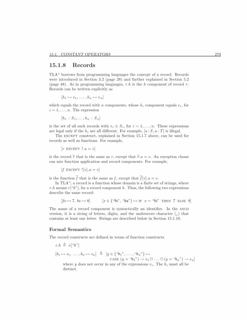
15.1. CONSTANT OPERATORS 279
15.1.8 Records
TLA+ borrows from programming languages the concept of a record. Recordswere introduced in Section 3.2 (page 28) and further explained in Section 5.2(page 48). As in programming languages, r .h is the h component of record r .Records can be written explicitly as
[h1 7→ e1, . . . , hn 7→ en ]
which equals the record with n components, whose hi component equals ei , fori = 1, . . . ,n. The expression
[h1 : S 1, . . . , hn : Sn ]
is the set of all such records with ei ∈ S i , for i = 1, . . . ,n. These expressionsare legal only if the hi are all different. For example, [a : S , a : T ] is illegal.
The except construct, explained in Section 15.1.7 above, can be used forrecords as well as functions. For example,
[r except !.a = e]
is the record r that is the same as r , except that r .a = e. An exception clausecan mix function application and record components. For example,
[f except ! [v ].a = e]
is the function f that is the same as f , except that f [v ].a = e.In TLA+, a record is a function whose domain is a finite set of strings, where
r .h means r [“h”], for a record component h. Thus, the following two expressionsdescribe the same record:
[fo 7→ 7, ba 7→ 8] [x ∈ {“fo”, “ba”} 7→ if x = “fo” then 7 else 8]
The name of a record component is syntactically an identifier. In the asciiversion, it is a string of letters, digits, and the underscore character (_) thatcontains at least one letter. Strings are described below in Section 15.1.10.
Formal Semantics
The record constructs are defined in terms of function constructs.
e.h ∆= e[“h”]
[h1 7→ e1, . . . , hn 7→ en ] ∆= [y ∈ {“h1”, . . . , “hn”} 7→case (y = “h1”)→ e1 2 . . . 2 (y = “hn”)→ en ]
where y does not occur in any of the expressions ei . The hi must all bedistinct.
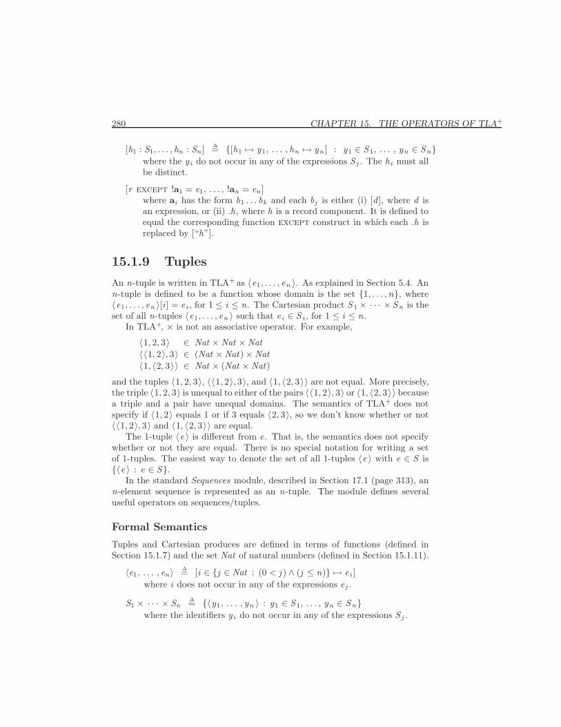
280 CHAPTER 15. THE OPERATORS OF TLA+
[h1 : S1, . . . , hn : Sn ] ∆= {[h1 7→ y1, . . . , hn 7→ yn ] : y1 ∈ S 1, . . . , yn ∈ Sn}where the y i do not occur in any of the expressions S j . The hi must allbe distinct.
[r except !a1 = e1, . . . , !an = en ]where ai has the form b1 . . . bk and each bj is either (i) [d ], where d isan expression, or (ii) .h, where h is a record component. It is defined toequal the corresponding function except construct in which each .h isreplaced by [“h”].
15.1.9 Tuples
An n-tuple is written in TLA+ as 〈e1, . . . , en 〉. As explained in Section 5.4. Ann-tuple is defined to be a function whose domain is the set {1, . . . ,n}, where〈e1, . . . , en 〉[i ] = ei , for 1 ≤ i ≤ n. The Cartesian product S 1 × · · · × Sn is theset of all n-tuples 〈e1, . . . , en 〉 such that ei ∈ S i , for 1 ≤ i ≤ n.
In TLA+, × is not an associative operator. For example,
〈1, 2, 3〉 ∈ Nat ×Nat ×Nat〈〈1, 2〉, 3〉 ∈ (Nat ×Nat)×Nat〈1, 〈2, 3〉〉 ∈ Nat × (Nat ×Nat)
and the tuples 〈1, 2, 3〉, 〈〈1, 2〉, 3〉, and 〈1, 〈2, 3〉〉 are not equal. More precisely,the triple 〈1, 2, 3〉 is unequal to either of the pairs 〈〈1, 2〉, 3〉 or 〈1, 〈2, 3〉〉 becausea triple and a pair have unequal domains. The semantics of TLA+ does notspecify if 〈1, 2〉 equals 1 or if 3 equals 〈2, 3〉, so we don’t know whether or not〈〈1, 2〉, 3〉 and 〈1, 〈2, 3〉〉 are equal.
The 1-tuple 〈e 〉 is different from e. That is, the semantics does not specifywhether or not they are equal. There is no special notation for writing a setof 1-tuples. The easiest way to denote the set of all 1-tuples 〈e 〉 with e ∈ S is{〈e 〉 : e ∈ S}.
In the standard Sequences module, described in Section 17.1 (page 313), ann-element sequence is represented as an n-tuple. The module defines severaluseful operators on sequences/tuples.
Formal Semantics
Tuples and Cartesian produces are defined in terms of functions (defined inSection 15.1.7) and the set Nat of natural numbers (defined in Section 15.1.11).
〈e1, . . . , en〉 ∆= [i ∈ {j ∈ Nat : (0 < j ) ∧ (j ≤ n)} 7→ ei ]where i does not occur in any of the expressions ej .
S1 × · · · × Sn∆= {〈y1, . . . , yn 〉 : y1 ∈ S 1, . . . , yn ∈ Sn}
where the identifiers y i do not occur in any of the expressions S j .
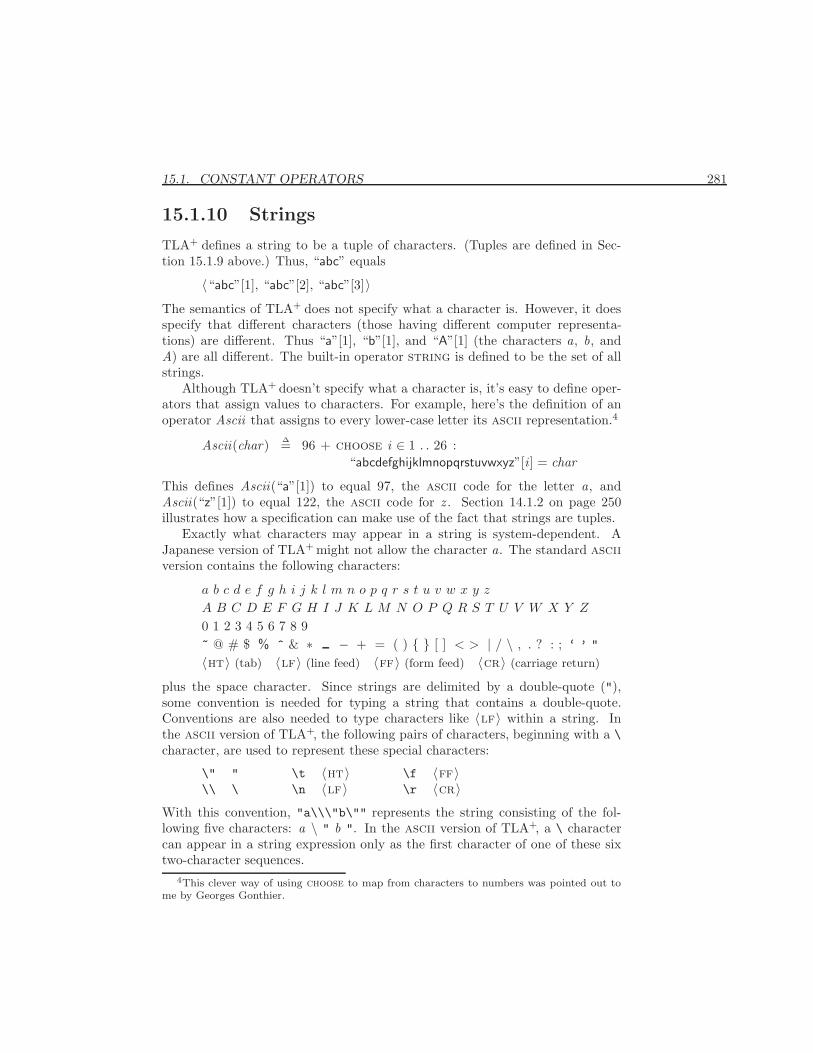
15.1. CONSTANT OPERATORS 281
15.1.10 Strings
TLA+ defines a string to be a tuple of characters. (Tuples are defined in Sec-tion 15.1.9 above.) Thus, “abc” equals
〈“abc”[1], “abc”[2], “abc”[3]〉The semantics of TLA+ does not specify what a character is. However, it doesspecify that different characters (those having different computer representa-tions) are different. Thus “a”[1], “b”[1], and “A”[1] (the characters a, b, andA) are all different. The built-in operator string is defined to be the set of allstrings.
Although TLA+ doesn’t specify what a character is, it’s easy to define oper-ators that assign values to characters. For example, here’s the definition of anoperator Ascii that assigns to every lower-case letter its ascii representation.4
Ascii(char) ∆= 96 + choose i ∈ 1 . . 26 :“abcdefghijklmnopqrstuvwxyz”[i ] = char
This defines Ascii(“a”[1]) to equal 97, the ascii code for the letter a, andAscii(“z”[1]) to equal 122, the ascii code for z . Section 14.1.2 on page 250illustrates how a specification can make use of the fact that strings are tuples.
Exactly what characters may appear in a string is system-dependent. AJapanese version of TLA+ might not allow the character a. The standard asciiversion contains the following characters:
a b c d e f g h i j k l m n o p q r s t u v w x y z
A B C D E F G H I J K L M N O P Q R S T U V W X Y Z
0 1 2 3 4 5 6 7 8 9~ @ # $ % ^ & ∗ − + = ( ) { } [ ] < > | / \ , . ? : ; ‘ ’ "
〈ht〉 (tab) 〈lf〉 (line feed) 〈ff〉 (form feed) 〈cr〉 (carriage return)
plus the space character. Since strings are delimited by a double-quote ("),some convention is needed for typing a string that contains a double-quote.Conventions are also needed to type characters like 〈lf〉 within a string. Inthe ascii version of TLA+, the following pairs of characters, beginning with a \character, are used to represent these special characters:
\" " \t 〈ht〉 \f 〈ff〉\\ \ \n 〈lf〉 \r 〈cr〉
With this convention, "a\\\"b\"" represents the string consisting of the fol-lowing five characters: a \ " b ". In the ascii version of TLA+, a \ charactercan appear in a string expression only as the first character of one of these sixtwo-character sequences.
4This clever way of using choose to map from characters to numbers was pointed out tome by Georges Gonthier.
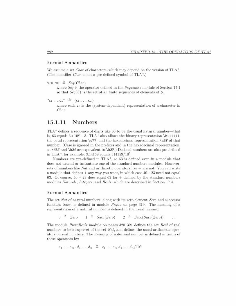
282 CHAPTER 15. THE OPERATORS OF TLA+
Formal Semantics
We assume a set Char of characters, which may depend on the version of TLA+.(The identifier Char is not a pre-defined symbol of TLA+.)
string∆= Seq(Char)
where Seq is the operator defined in the Sequences module of Section 17.1so that Seq(S ) is the set of all finite sequences of elements of S .
“c1 . . . cn”∆= 〈c1, . . . , cn 〉
where each ci is the (system-dependent) representation of a character inChar .
15.1.11 Numbers
TLA+ defines a sequence of digits like 63 to be the usual natural number—thatis, 63 equals 6 ∗ 102 + 3. TLA+ also allows the binary representation \b111111,the octal representation \o77, and the hexadecimal representation \h3F of thatnumber. (Case is ignored in the prefixes and in the hexadecimal representation,so \H3F and \h3f are equivalent to \h3F.) Decimal numbers are also pre-definedin TLA+; for example, 3.14159 equals 314159/105.
Numbers are pre-defined in TLA+, so 63 is defined even in a module thatdoes not extend or instantiate one of the standard numbers modules. However,sets of numbers like Nat and arithmetic operators like + are not. You can writea module that defines + any way you want, in which case 40+23 need not equal63. Of course, 40 + 23 does equal 63 for + defined by the standard numbersmodules Naturals , Integers , and Reals , which are described in Section 17.4.
Formal Semantics
The set Nat of natural numbers, along with its zero element Zero and successorfunction Succ, is defined in module Peano on page 319. The meaning of arepresentation of a natural number is defined in the usual manner:
0 ∆= Zero 1 ∆= Succ(Zero) 2 ∆= Succ(Succ(Zero)) . . .
The module ProtoReals module on pages 320–321 defines the set Real of realnumbers to be a superset of the set Nat , and defines the usual arithmetic oper-ators on real numbers. The meaning of a decimal number is defined in terms ofthese operators by:
c1 · · · cm . d1 · · · dn∆= c1 · · · cm d1 · · · dn/10n
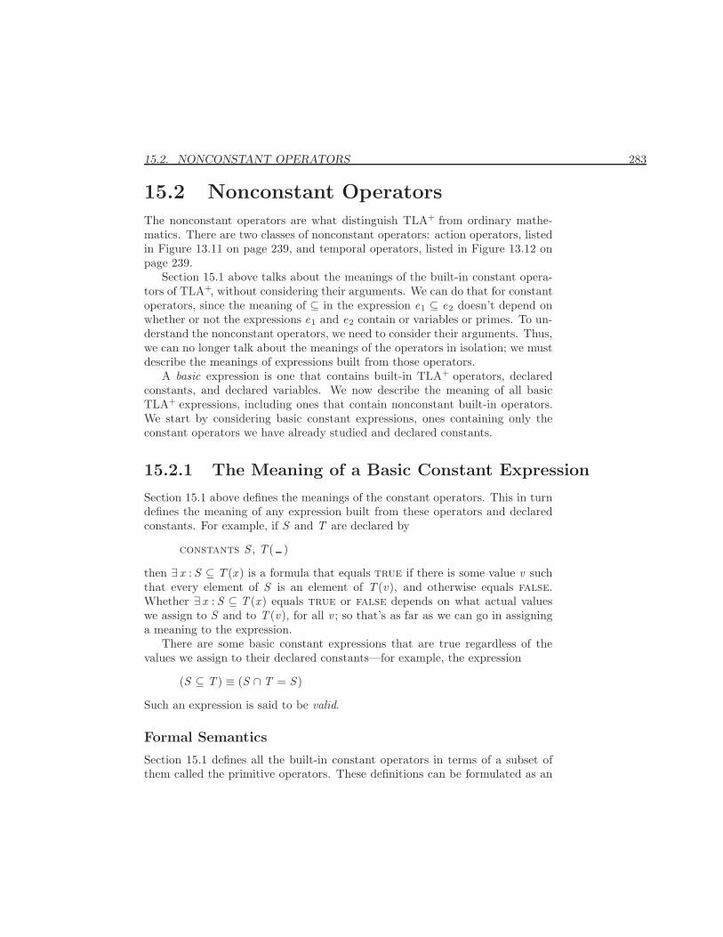
15.2. NONCONSTANT OPERATORS 283
15.2 Nonconstant Operators
The nonconstant operators are what distinguish TLA+ from ordinary mathe-matics. There are two classes of nonconstant operators: action operators, listedin Figure 13.11 on page 239, and temporal operators, listed in Figure 13.12 onpage 239.
Section 15.1 above talks about the meanings of the built-in constant opera-tors of TLA+, without considering their arguments. We can do that for constantoperators, since the meaning of ⊆ in the expression e1 ⊆ e2 doesn’t depend onwhether or not the expressions e1 and e2 contain or variables or primes. To un-derstand the nonconstant operators, we need to consider their arguments. Thus,we can no longer talk about the meanings of the operators in isolation; we mustdescribe the meanings of expressions built from those operators.
A basic expression is one that contains built-in TLA+ operators, declaredconstants, and declared variables. We now describe the meaning of all basicTLA+ expressions, including ones that contain nonconstant built-in operators.We start by considering basic constant expressions, ones containing only theconstant operators we have already studied and declared constants.
15.2.1 The Meaning of a Basic Constant Expression
Section 15.1 above defines the meanings of the constant operators. This in turndefines the meaning of any expression built from these operators and declaredconstants. For example, if S and T are declared by
constants S , T ( )
then ∃ x : S ⊆ T (x ) is a formula that equals true if there is some value v suchthat every element of S is an element of T (v), and otherwise equals false.Whether ∃ x : S ⊆ T (x ) equals true or false depends on what actual valueswe assign to S and to T (v), for all v ; so that’s as far as we can go in assigninga meaning to the expression.
There are some basic constant expressions that are true regardless of thevalues we assign to their declared constants—for example, the expression
(S ⊆ T ) ≡ (S ∩T = S )
Such an expression is said to be valid.
Formal Semantics
Section 15.1 defines all the built-in constant operators in terms of a subset ofthem called the primitive operators. These definitions can be formulated as an
284 CHAPTER 15. THE OPERATORS OF TLA+
inductive set of rules that define the meaning [[c]] of any basic constant expressionc. For example, from the definition
e /∈ S ∆= ¬(e ∈ S )
we get the rule
[[e /∈ S ]] = ¬([[e]] ∈ [[S ]])
These rules define the meaning of a basic constant expression to be an expressioncontaining only primitive constant operators and declared constants.
If S and T are constants declared as above, then the meaning [[∃ x : S ⊆ T (x )]]of the expression ∃ x : S ⊆ T (x ) is the expression itself. Logicians usually carrythings further, assigning some meanings [[S ]] and [[T ]] to declared constants anddefining [[∃ x : S ⊆ T (x )]] to equal ∃ x : [[S ]] ⊆ [[T ]](x ). For simplicity, I have short-circuited that extra level of meaning.
I am taking as given the meaning of an expression containing only primitiveconstant operators and declared constants. In particular, I take as primitivethe notion of validity for such expressions. Section 15.1 defines the meaning ofany basic constant expression in terms of these expressions, so it defines whatit means for a basic constant expression to be valid.
15.2.2 The Meaning of a State Function
A state is an assignment of values to variables. (In ZF set theory, on which thesemantics of TLA+ is based, value is just another term for set.) States werediscussed in Sections 2.1 and 2.3.
A state function is an expression that is built from declared variables, de-clared constants, and constant operators. (State functions can also containenabled expressions, which are described below.) State functions are discussedon page 25 of Section 3.1. A state function assigns a constant expression toevery state. If state function e assigns to state s the constant v , then we saythat v is the value of e in state s . For example, if x is a declared variable, Tis a declared constant, and s is a state that assigns to x the value 42; then thevalue of x ∈ T in state s is the constant expression 42 ∈ T . A state function isvalid iff it has the value true in every state.
Formal Semantics
A state is an assignment of values to variables. Formally, a state s is a functionwhose domain is the set of all variable names, where s [“x”] is the value that sassigns to variable x . We write s [[x ]] instead of s [“x”].
A basic state function is an expression that is built from declared variables,declared constants, constant operators, and enabled expressions, which are
15.2. NONCONSTANT OPERATORS 285
expressions of the form Enabled e. An enabled-free basic state function is,obviously, one with no enabled expressions. The meaning of a basic statefunction is a mapping from states to values. We let s [[e]] be the value that statefunction e assigns to a state s . Since a variable is a state function, we thus sayboth that state s assigns s [[x ]] to variable x , and that the state function x assignss [[x ]] to state s . A basic state function e is defined to be valid iff s [[e]] is validfor all states s .
Using the meanings assigned to the constant operators in Section 15.1 above,we inductively define s [[e]] for any enabled-free state function e to be an ex-pression built from the primitive TLA+ constant operators, declared constants,and the values assigned by s to each variable. For example, if x is a variableand S is a constant, then
s [[x /∈ S ]] = ¬(s [[x ]] ∈ S )
It is easy to see that s [[c]] to equal [[c]], for any constant expression c. (Thisexpresses formally that a constant has the same value in all states.)
To define the meaning of all basic state function, not just enabled-free ones,we must define the meaning of an enabled expression. This is done below.
I described the meaning of a state function as a “mapping” on states. Thismapping cannot be a function, because there is no set of all states. Since forany set S there is a state that assigns the value S to each variable, there are toomany states to form a set. (See the discussion of Russell’s paradox on page 66.)To be strictly formal, I should explain what I’m doing as follows. I define anoperator M such that, if s is a state and e is a syntactically correct basic statefunction, then M (s , e), which I write s [[e]], is the basic constant expression thatis the meaning of e in state s .
Actually, this description of the semantics isn’t right either. A state is amapping from variables to values (sets), not to constant expressions. Sincethere are an uncountable number of sets and only a countable number of finitesequences of strings, there are values that can’t be described by any expression.Suppose ξ is such a value, and let s be a state that assigns the value ξ to thevariable x . Then s [[x = {}]] equals ξ = {}, which isn’t a constant expressionbecause ξ isn’t an expression. So, to be really formal, I would have to define asemantic constant expression to be one made from primitive constant operators,declared constants, and arbitrary values. The meaning of a basic state functionis a mapping from states to semantic constant expressions.
I won’t bother with these details, which are needed for a really formal defi-nition of the semantics. I will instead define a semi-formal semantics for basicexpression that I hope is easier to understand. Mathematically sophisticatedreaders who understand the less formal exposition should be able to fill in themissing formal details.
286 CHAPTER 15. THE OPERATORS OF TLA+
15.2.3 Action Operators
A transition function is an expression built from state functions using the prim-ing operator (′) and the other action operators of TLA+ listed in Figure 13.11on page 239. A transition function assigns a value to every step, where a step isa pair of states. In a transition function, an unprimed occurrence of a variablex represents the value of x in the first (old) state, and a primed occurrence ofx represents its value in the second (new) state. For example, if state s assignsthe value 4 to x and state t assigns the value 5 to x , then transition functionx ′ − x assigns to the step s → t the value 5− 4, which of course equals 1.
An action is a Boolean-valued transition function, such as x ′ > x . We saythat action A is true on step s → t , or that s → t is an A step, iff A assigns thevalue true to s → t . An action is said to be valid iff it is true on any step.
The action operators of TLA+ other than ′ have the following meanings,where A and B are actions.
[A]e equals A ∨ (e ′ = e).
〈A〉e equals A ∧ (e ′ 6= e).
Enabled A is the state function that is true in state s iff there is some statet such that s → t is an A step. true.
unchanged e equals e ′ = e, for any state function e.
A · B is the action that is true on step s → t iff there is a state u such thats → u is an A step and u → t is a B step.
Priming and the construct [A]v are introduced in Section 2.2 (page 15); theunchanged operator is introduced on page 26 of Section 3.1 (24); enabled isintroduced on page 92 of Section 8.2; the construct 〈A〉v is defined on page 90 ofSection 8.1; and the action-composition operator “·” is introduced in Section 7.3(page 76).
Formal Semantics
A basic transition function is a basic expression that does not contain any tem-poral operators. The meaning of a basic transition function e is an assignmentof a basic constant expression 〈s , t 〉[[e]] to any pair of states 〈s , t 〉. (I use herethe more conventional notation 〈s , t 〉 instead of s → t .) A transition functionis valid iff 〈s , t 〉[[e]] is valid, for all states s and t .
If e is a basic state function, then we interpret e as a basic transition functionby defining 〈s , t 〉[[e]] to equal s [[e]]. As indicated above, unchanged and theconstructs [A]e and 〈A〉e are defined in terms of priming. To define the meaningsof the remaining action operators, we first define existential quantification overall states. Let IsAState be an operator such that IsAState(s) is true iff s is a
15.2. NONCONSTANT OPERATORS 287
state—that is, a function whose domain is the set of all variable names. (It’s easyto define IsAState using the operator IsAFcn, defined on page 277.) Existentialquantification over all states is then defined by
∃ state s : p ∆= ∃ s : IsAState(s) ∧ p
for any formula p. The meanings of all transition functions and all state functions(including enabled expressions) is then defined inductively by the definitionsalready given and the following definitions of the remaining action operators:
e ′ is the transition function defined by 〈s , t 〉[[e′]] ∆= t [[e]] for any statefunction e.
Enabled A is the state function defined by
s [[Enabled A]] ∆= ∃ state t : 〈s , t 〉[[A]]
for any transition function A.
A · B is the transition function defined by
〈s , t 〉[[A · B ]] ∆= ∃ state u : 〈s , u 〉[[A]] ∧ 〈u, t 〉[[B ]]
for any transition functions A and B .
The formal semantics talks about transition functions, not actions. Since TLA+
is typeless, there is no formal distinction between an action and an arbitrarytransition function. We could define an action A to be a transition functionsuch that 〈s , t 〉[[A]] is a Boolean for all states s and t . However, what we usuallymean by an action is a transition function A such that 〈s , t 〉[[A]] is a Bool-ean whenever s and t are reachable states of some specification. For example,consider a specification with a variable b of type boolean might contain an Types are ex-
plained onpage 25.
“action” b ∧ (y ′ = y). We can calculate the meaning of Enabled (b ∧ (y ′ = y)as follows:
s [[Enabled (b ∧ (y ′ = y)]]= ∃ state t : 〈s , t 〉[[b ∧ (y ′ = y)]] By definition of enabled.
= ∃ state t : 〈s , t 〉[[b]] ∧ (〈s , t 〉[[y ′]] = 〈s , t 〉[[y]]) By definition of ∧ and =.
= ∃ state t : s [[b]] ∧ (t [[y]] = s [[y]]) By definition of ′, since 〈s, t 〉[[e]] = efor any state function e.
If s [[b]] is a Boolean, we can use the rules of ordinary logic to simplify the lastexpression and obtain:
s [[Enabled (b ∧ (y ′ = y)]] = s [[b]]
However, if s is a state that assigns the value 2 to the variable b and the value−7 to the variable y, then
s [[Enabled (b ∧ (y ′ = y)]] = ∃ state t : 2 ∧ (t [[y]] = −7)
288 CHAPTER 15. THE OPERATORS OF TLA+
The last expression may or may not equal 2. (See Section 15.1.3 on page 270.)If the specification we are writing makes sense, it can depend on the meaningof Enabled (b ∧ (y ′ = y) only for states in which the value of b is a Boolean.We don’t care about its value on a state that assigns to b the value 2, just aswe don’t care about the value of 3/x in a state that assigns the value “abc” tox . See the discussion of silly expressions in Section 6.2 (page 67).
15.2.4 Temporal Operators
As explained in Section 8.1, a temporal formula F is true or false on a behavior,where a behavior is a sequence of states. The syntax of temporal formulas is de-fined inductively to be all formulas having one of the forms shown in Figure 13.12on page 239, where e is a state function, A is an action, and F and G are tempo-ral formulas. All these temporal operators are explained in Chapter 8—exceptfor +−., which is explained in Chapter 10.7.
The formula 2F is true for a behavior σ iff the temporal formula F is truefor σ and all suffixes of σ. To define the constructs 2[A]e and 3〈A〉e , we regardan action B to be a temporal formula that is true of a behavior σ iff the firsttwo states of σ form a B step. Thus, 2[A]e is true of σ iff every successive pairof states of σ is a [A]e step. All the other temporal operators of TLA+, except∃∃∃∃∃∃ , ∀ , and +−., are defined as follows in terms of 2:
3F ∆= ¬2¬FWFe(A) ∆= 23¬(Enabled 〈A〉e) ∨ 23〈A〉eSFe(A) ∆= 32¬(Enabled 〈A〉e) ∨ 23〈A〉eF ; G ∆= 2(F ⇒ 3G)¬F
The temporal existential quantifier ∃∃∃∃∃∃ is a hiding operator, ∃∃∃∃∃∃ x : F meaningformula F with the variable x hidden. To define this more precisely, we firstdefine \σ to be the (possibly finite) sequence of states obtained by removingfrom σ all stuttering steps—that is, by removing any state that is the same asthe previous one. We then define σ∼x τ to be true iff \σ and \τ are the sameexcept for the values that their states assign to the variable x . Finally, ∃∃∃∃∃∃ x : Fis defined to be true for a behavior σ iff F is true for some behavior τ such thatσ∼x τ .
The temporal universal quantifier ∀∀∀∀∀∀ is defined in terms of ∃∃∃∃∃∃ by
∀∀∀∀∀∀ x : F ∆= ¬(∃∃∃∃∃∃ x : ¬F )
The formula F +−. G asserts that G does not become false before F does.More precisely, we define a formula H to be true for a finite prefix ρ of a behaviorσ iff H is true for some (infinite) behavior that extends ρ. (In particular, H istrue of the empty prefix iff H satisfies some behavior.) Then F +−. G is definedto be true for a behavior σ iff (i) F ⇒ G is true for σ and (ii) for every finite
15.2. NONCONSTANT OPERATORS 289
prefix ρ of σ, if F is true for ρ then G is true for the prefix of σ that is one statelonger than ρ.
Formal Semantics
Formally, a behavior is a function from the set Nat of natural numbers to states.(We think of σ as the sequence σ[0], σ[1], . . . of states.) The meaning of atemporal formula is a predicate on behaviors—that is, a mapping from behaviorsto Booleans. We write σ |= F for the value that the meaning of F assigns to thebehavior σ. The temporal formula F is valid iff σ |= F is valid, for all behaviorsσ.
Above, we have defined all the other temporal operators in terms of 2, ∃∃∃∃∃∃ ,and +−.. Formally, since an action is not a temporal formula, the construct 2[A]eis not an instance of the temporal operator 2, so its meaning should be definedseparately. The construct 3〈A〉e , which is similarly not an instance of 3, isthen defined to equal ¬2[¬A]e .
To define the meaning of 2, we first define σ+n to be the behavior obtainedby deleting the first n states of σ:
σ+n ∆= [i ∈ Nat 7→ σ[i + n] ]
We then define the meaning of 2 as follows, for any temporal formula F , tran-sition function A and state function e:
σ |= 2F ∆= ∀n ∈ Nat : σ+n |= Fσ |= 2[A]e
∆= ∀n ∈ Nat : 〈σ[n], σ[n + 1]〉[[[A]e ]]
To formalize the definition of ∃∃∃∃∃∃ given above, we first define \ by:
\σ∆= let f [n ∈ Nat ] ∆= if n = 0
then 0else if σ[n] = σ[n − 1] then f [n − 1]
else f [n − 1] + 1S ∆= {f [n] : n ∈ Nat}
in [n ∈ S 7→ σ[choose i ∈ Nat : f [i ] = n] ]
Next, let sx←v be the state that is the same as state s except that it assigns tothe variable x the value v . We then define ∼x by:
σ∼x τ∆= \σ = [n ∈ domain \τ 7→ τx←σ[n][[x ]]]
We next define existential quantification over behaviors. This is done much aswe defined quantification over states on pages 286–287 above; we first defineIsABehavior so that IsABehavior(σ) is true iff σ is a behavior, and we thendefine:
∃ behavior σ : F ∆= ∃σ : IsABehavior(σ) ∧ F
290 CHAPTER 15. THE OPERATORS OF TLA+
We can now define the meaning of ∃∃∃∃∃∃ by:
σ |= ∃∃∃∃∃∃ x : F ∆= ∃ behavior τ : (σ∼x τ) ∧ (τ |= F )
Finally, we define the meaning of +−. as follows:
σ |= F +−. G ∆=let PrefixSat(n,H ) ∆= ∃ behavior τ : ∧ ∀ i ∈ 0 . . (n − 1) : τ [i ] = σ[i ]
∧ τ |= Hin ∧ σ |= F ⇒ G
∧ ∀n ∈ Nat : PrefixSat(n,F )⇒ PrefixSat(n + 1,G)
Chapter 16
The Meaning of a Module
Chapter 15 defines the meaning of the built-in TLA+ operators. In doing so, itdefines the meaning of a basic expression—that is, of an expression containingonly built-in operators, declared constants, and declared variables. We nowdefine the meaning of a module in terms of basic expressions. Since a TLA+
specification consists of a collection of modules, this defines the semantics ofTLA+.
We also complete the definition of the syntax of TLA+ by giving the remain-ing context-dependent syntactic conditions not described in Chapter 14. Here’sa list of some illegal expressions that satisfy the grammar of Chapter 14, andwhere in this chapter you can find the conditions that make them illegal.
• F (x ), if F is defined by F (x , y) ∆= x + y (Section 16.1)
• (x ′ + 1)′ (Section 16.2)
• x + 1, if x is not defined or declared (Section 16.3)
• F ∆= 0, if F is already defined (Section 16.5)
This chapter is meant to be read in its entirety. To try to make it as readableas possible, I have made the exposition somewhat informal. Wherever I could,I have used examples in place of formal definitions. The examples assume thatyou understand the approximate meanings of the TLA+ constructs, as explainedin Part I. I hope that mathematically sophisticated readers will see how to fillin the missing formalism.
16.1 Operators and Expressions
Because it uses conventional mathematical notation, TLA+ has a rather richsyntax, with several different ways of expressing the same basic type of math-
291
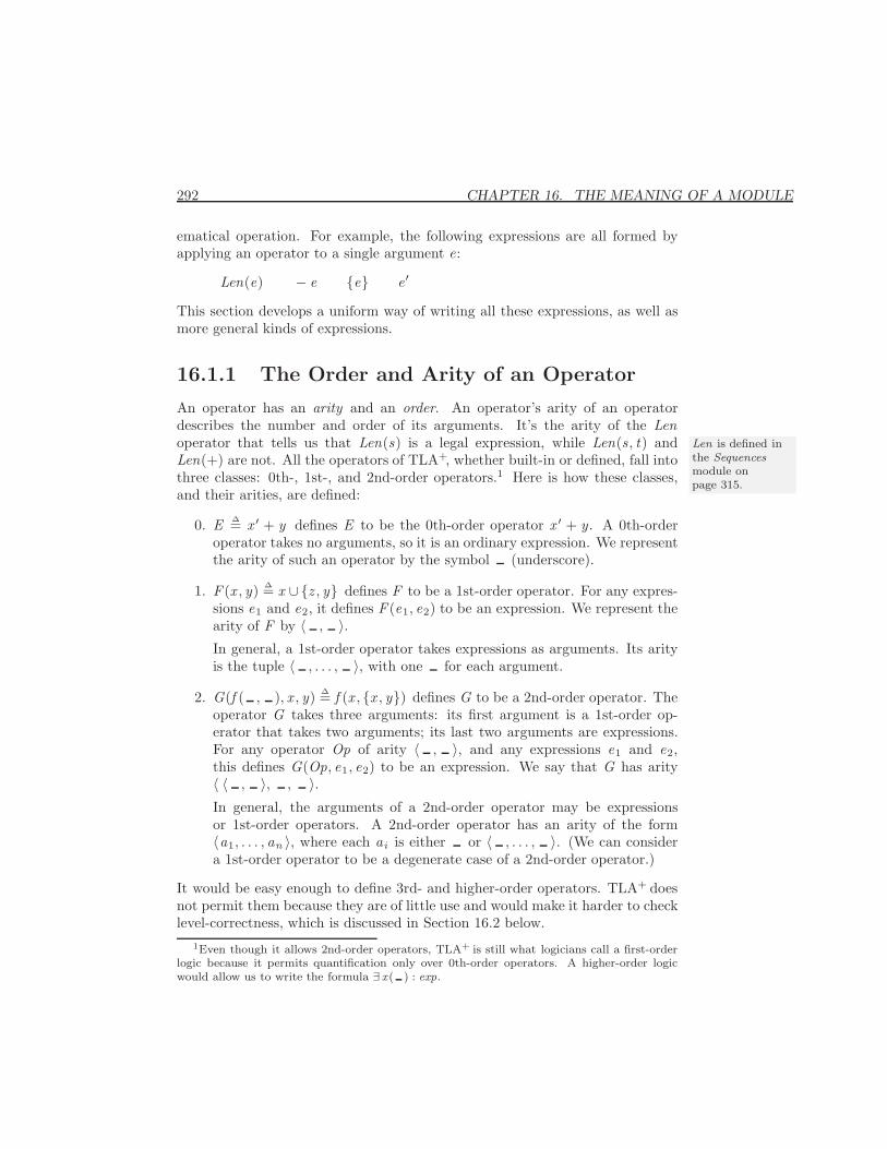
292 CHAPTER 16. THE MEANING OF A MODULE
ematical operation. For example, the following expressions are all formed byapplying an operator to a single argument e:
Len(e) − e {e} e ′
This section develops a uniform way of writing all these expressions, as well asmore general kinds of expressions.
16.1.1 The Order and Arity of an Operator
An operator has an arity and an order. An operator’s arity of an operatordescribes the number and order of its arguments. It’s the arity of the Lenoperator that tells us that Len(s) is a legal expression, while Len(s , t) and Len is defined in
the Sequencesmodule onpage 315.
Len(+) are not. All the operators of TLA+, whether built-in or defined, fall intothree classes: 0th-, 1st-, and 2nd-order operators.1 Here is how these classes,and their arities, are defined:
0. E ∆= x ′ + y defines E to be the 0th-order operator x ′ + y. A 0th-orderoperator takes no arguments, so it is an ordinary expression. We representthe arity of such an operator by the symbol (underscore).
1. F (x , y) ∆= x ∪{z , y} defines F to be a 1st-order operator. For any expres-sions e1 and e2, it defines F (e1, e2) to be an expression. We represent thearity of F by 〈 , 〉.In general, a 1st-order operator takes expressions as arguments. Its arityis the tuple 〈 , . . . , 〉, with one for each argument.
2. G(f ( , ), x , y) ∆= f (x , {x , y}) defines G to be a 2nd-order operator. Theoperator G takes three arguments: its first argument is a 1st-order op-erator that takes two arguments; its last two arguments are expressions.For any operator Op of arity 〈 , 〉, and any expressions e1 and e2,this defines G(Op, e1, e2) to be an expression. We say that G has arity〈 〈 , 〉, , 〉.In general, the arguments of a 2nd-order operator may be expressionsor 1st-order operators. A 2nd-order operator has an arity of the form〈a1, . . . , an 〉, where each ai is either or 〈 , . . . , 〉. (We can considera 1st-order operator to be a degenerate case of a 2nd-order operator.)
It would be easy enough to define 3rd- and higher-order operators. TLA+ doesnot permit them because they are of little use and would make it harder to checklevel-correctness, which is discussed in Section 16.2 below.
1Even though it allows 2nd-order operators, TLA+ is still what logicians call a first-orderlogic because it permits quantification only over 0th-order operators. A higher-order logicwould allow us to write the formula ∃ x( ) : exp.
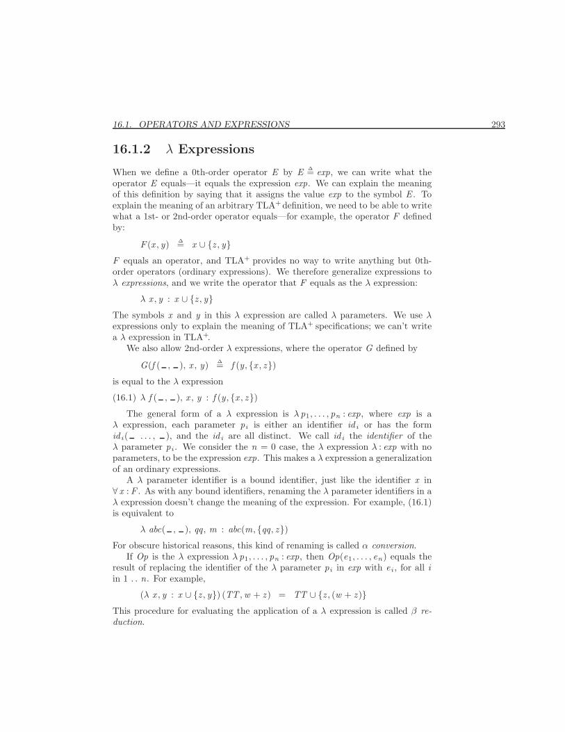
16.1. OPERATORS AND EXPRESSIONS 293
16.1.2 λ Expressions
When we define a 0th-order operator E by E ∆= exp, we can write what theoperator E equals—it equals the expression exp. We can explain the meaningof this definition by saying that it assigns the value exp to the symbol E . Toexplain the meaning of an arbitrary TLA+ definition, we need to be able to writewhat a 1st- or 2nd-order operator equals—for example, the operator F definedby:
F (x , y) ∆= x ∪ {z , y}F equals an operator, and TLA+ provides no way to write anything but 0th-order operators (ordinary expressions). We therefore generalize expressions toλ expressions, and we write the operator that F equals as the λ expression:
λ x , y : x ∪ {z , y}The symbols x and y in this λ expression are called λ parameters. We use λexpressions only to explain the meaning of TLA+ specifications; we can’t writea λ expression in TLA+.
We also allow 2nd-order λ expressions, where the operator G defined by
G(f ( , ), x , y) ∆= f (y, {x , z})is equal to the λ expression
λ f ( , ), x , y : f (y, {x , z})(16.1)
The general form of a λ expression is λ p1, . . . , pn : exp, where exp is aλ expression, each parameter pi is either an identifier id i or has the formid i( . . . , ), and the id i are all distinct. We call id i the identifier of theλ parameter pi . We consider the n = 0 case, the λ expression λ : exp with noparameters, to be the expression exp. This makes a λ expression a generalizationof an ordinary expressions.
A λ parameter identifier is a bound identifier, just like the identifier x in∀ x : F . As with any bound identifiers, renaming the λ parameter identifiers in aλ expression doesn’t change the meaning of the expression. For example, (16.1)is equivalent to
λ abc( , ), qq, m : abc(m, {qq, z})For obscure historical reasons, this kind of renaming is called α conversion.
If Op is the λ expression λ p1, . . . , pn : exp, then Op(e1, . . . , en) equals theresult of replacing the identifier of the λ parameter pi in exp with ei , for all iin 1 . . n. For example,
(λ x , y : x ∪ {z , y}) (TT ,w + z ) = TT ∪ {z , (w + z )}This procedure for evaluating the application of a λ expression is called β re-duction.
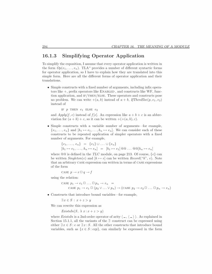
294 CHAPTER 16. THE MEANING OF A MODULE
16.1.3 Simplifying Operator Application
To simplify the exposition, I assume that every operator application is written inthe form Op(e1, . . . , en). TLA+ provides a number of different syntactic formsfor operator application, so I have to explain how they are translated into thissimple form. Here are all the different forms of operator application and theirtranslations.
• Simple constructs with a fixed number of arguments, including infix opera-tors like +, prefix operators like Enabled , and constructs like WF, func-tion application, and if/then/else. These operators and constructs poseno problem. We can write +(a, b) instead of a + b, IfThenElse(p, e1 , e2)instead of
if p then e1 else e2
and Apply(f , e) instead of f [e]. An expression like a + b + c is an abbre-viation for (a + b) + c, so it can be written +(+(a, b), c).
• Simple constructs with a variable number of arguments—for example,{e1, . . . , en} and [h1 7→ e1, . . . , hn 7→ en ]. We can consider each of theseconstructs to be repeated application of simpler operators with a fixednumber of arguments. For example,
{e1, . . . , en} = {e1} ∪ . . . ∪ {en}[h1 7→ e1, . . . , hn 7→ en ] = [h1 7→ e1] @@ . . . @@[hn 7→ en ]
where @@ is defined in the TLC module, on page 213. Of course, {e} canbe written Singleton(e) and [h 7→ e] can be written Record(“h”, e). Notethat an arbitrary case expression can written in terms of case expressionsof the form
case p → e 2 q → f
using the relation:
case p1 → e1 2 . . . 2 pn → en =case p1 → e1 2 (p2 ∨ . . . ∨ pn)→ (case p2 → e2 2 . . . 2 pn → en)
• Constructs that introduce bound variables—for example,
∃ x ∈ S : x + z > y
We can rewrite this expression as
ExistsIn(S , λ x : x + z > y)
where ExistsIn is a 2nd-order operator of arity 〈 , 〈 〉 〉. As explained inSection 15.1.1, all the variants of the ∃ construct can be expressed usingeither ∃ x ∈ S : e or ∃ x : S . All the other constructs that introduce boundvariables, such as {x ∈ S : exp}, can similarly be expressed in the form
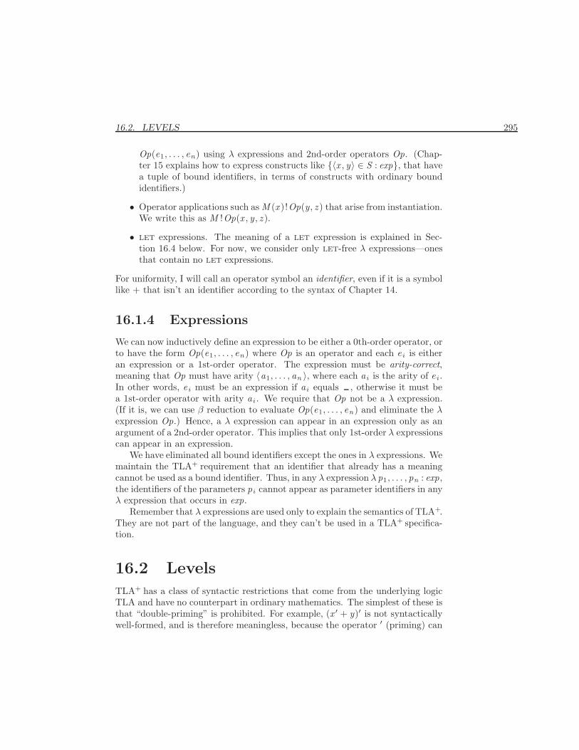
16.2. LEVELS 295
Op(e1, . . . , en) using λ expressions and 2nd-order operators Op. (Chap-ter 15 explains how to express constructs like {〈x , y〉 ∈ S : exp}, that havea tuple of bound identifiers, in terms of constructs with ordinary boundidentifiers.)
• Operator applications such as M (x )!Op(y, z ) that arise from instantiation.We write this as M !Op(x , y, z ).
• let expressions. The meaning of a let expression is explained in Sec-tion 16.4 below. For now, we consider only let-free λ expressions—onesthat contain no let expressions.
For uniformity, I will call an operator symbol an identifier, even if it is a symbollike + that isn’t an identifier according to the syntax of Chapter 14.
16.1.4 Expressions
We can now inductively define an expression to be either a 0th-order operator, orto have the form Op(e1, . . . , en) where Op is an operator and each ei is eitheran expression or a 1st-order operator. The expression must be arity-correct,meaning that Op must have arity 〈a1, . . . , an 〉, where each ai is the arity of ei .In other words, ei must be an expression if ai equals , otherwise it must bea 1st-order operator with arity ai . We require that Op not be a λ expression.(If it is, we can use β reduction to evaluate Op(e1, . . . , en) and eliminate the λexpression Op.) Hence, a λ expression can appear in an expression only as anargument of a 2nd-order operator. This implies that only 1st-order λ expressionscan appear in an expression.
We have eliminated all bound identifiers except the ones in λ expressions. Wemaintain the TLA+ requirement that an identifier that already has a meaningcannot be used as a bound identifier. Thus, in any λ expression λ p1, . . . , pn : exp,the identifiers of the parameters pi cannot appear as parameter identifiers in anyλ expression that occurs in exp.
Remember that λ expressions are used only to explain the semantics of TLA+.They are not part of the language, and they can’t be used in a TLA+ specifica-tion.
16.2 Levels
TLA+ has a class of syntactic restrictions that come from the underlying logicTLA and have no counterpart in ordinary mathematics. The simplest of these isthat “double-priming” is prohibited. For example, (x ′ + y)′ is not syntacticallywell-formed, and is therefore meaningless, because the operator ′ (priming) can
296 CHAPTER 16. THE MEANING OF A MODULE
be applied only to a state function, not to a transition function like x ′+ y. Thisclass of restriction is expressed in terms of levels.
In TLA, an expression has one of four basic levels, which are numbered 0,1, 2, and 3. These levels are described below, using examples that assume x , y,and c are declared by
variables x , y constant c
and symbols like + have their usual meanings.
0. A constant -level expression is a constant; it contains only constants andconstant operators. Example: c + 3.
1. A state-level expression is a state function; it may contain constants, con-stant operators, and unprimed variables. Example: x + 2 ∗ c.
2. A transition-level expression is a transition function; it may contain any-thing except temporal operators. Example: x ′ + y > c.
3. A temporal -level expression is a temporal formula; it may contain any TLAoperator. Example: 2[x ′ > y + c]〈x , y 〉.
Chapter 15 assigns meanings to all basic expressions—ones containing only thebuilt-in operators of TLA+ and declared constants and variables. The meaningassigned to an expression depends as follows on its level.
0. The meaning of a constant-level basic expression is a constant-level basicexpression containing only primitive operators.
1. The meaning of a state-level basic expression is an assignment of a constantexpression s [[e]] to any state s .
2. The meaning of a transition-level basic expression e is an assignment of aconstant expression 〈s , t 〉[[e]] to any transition s → t .
3. The meaning of a temporal-level basic expression F is an assignment of aconstant expression σ |= F to any behavior σ.
An expression of any level can be considered to be an expression of a higher level,except that a transition-level expression is not a temporal-level expression.2 Forexample, if x is a declared variable, then the state-level expression x > 2 is thetemporal-level formula such that σ |= x is the value of x > 2 in the first state ofσ, for any behavior σ.3
A set of simple rules inductively defines whether a basic expression is level-correct and, if so, what its level is. Here are some of the rules:
2More precisely, a transition-level expression that is not a state-level expression is not atemporal-level expression.
3The expression x + 2 can be considered to be a temporal-level expression that, like thetemporal-level expression 2(x + 2), is silly. (See the discussion of silliness in Section 6.2 onpage 67.)
16.2. LEVELS 297
• A declared constant is a level-correct expression of level 0.
• A declared variable is a level-correct expression of level 1.
• If Op is declared to be a 1st-order constant operator, then the expressionOp(e1, . . . , en) is level-correct iff each ei is level correct, in which case itslevel is the maximum of the levels of the ei .
• e1 ∈ e2 is level correct iff e1 and e2 are, in which case its level is themaximum of the levels of e1 and e2.
• e ′ is level-correct, and has level 2, iff e is level-correct and has level atmost 1.4
• Enabled e is level-correct, and has level 1, iff e is level-correct and haslevel at most 2.
• ∃ x : e is level-correct, and has level l , iff e is level-correct and has level l ,when x is considered to be a declared constant.
• ∃∃∃∃∃∃ x : e is level-correct, and has level 3, iff e is level-correct and has anylevel other than 2, when x is considered to be a declared variable.
There are additional rules for the other TLA+ operators. They should be obvi-ous.
A useful consequence of the rules is that level-correctness of a basic expressiondoes not depend on the levels of the declared identifiers. In other words, anexpression e is level-correct when c is declared to be a constant iff it is level-correct when c is declared to be a variable. Of course, the level of e may dependon the level of c.
We can abstract these rules by generalizing the concept of a level. So far, Ihave defined the level only of an expression. I now define the level of a 1st- or2nd-order operator Op to be a rule for determining the level-correctness and levelof an expression Op(e1, . . . , en) as a function of the levels of the arguments ei .The level of a 1st-order operator is a rule, so the level of a 2nd-order operator Opis a rule that depends in part on rules—namely, on the levels of the argumentsthat are operators. This makes a rigorous general definition of levels for 2nd-order operators rather complicated. Fortunately, there’s a simpler, less generaldefinition that handles all the operators of TLA+. Even more fortunately, youdon’t have to know it, so I won’t bother writing it down. All you need to knowis that there exists a way of assigning a level to every built-in operator of TLA+.The level-correctness and level of any basic expression is then determined bythose levels and the levels of the declared identifiers that occur in the expression.
4If e is a constant expression, then e′ equals e, so we could consider e′ to have level 0. Forsimplicity, we consider e′ to have level 2 even if e is a constant.
298 CHAPTER 16. THE MEANING OF A MODULE
One important class of operator levels are the constant levels. Any expressionbuilt from constant-level operators and declared constants has constant level.The built-in constant operators of TLA+, listed in Figures 13.10 and 13.10 (pages239 and 239) all have constant level. Any operator defined solely in terms ofconstant-level operators and declared constants has constant level.
We now extend the definition of level-correctness from expressions to λ ex-pressions. We define the λ expression λp1, . . . , pn : exp to be level-correct iff expis level-correct when the λ parameter identifiers are declared to be constantsof the appropriate arity. For example, λp, q( ) : exp is level-correct iff exp islevel-correct with the additional declaration:
constants p, q( )
This inductively defines level-correctness for λ expressions. The definition isreasonable because, as observed a couple of paragraphs ago, the level-correctnessof exp doesn’t depend on whether we assign level 0 or 1 to the λ parameters.One can also define the level of an arbitrary λ expression, but that would requirethe general definition of the level of an operator, whose complexity we want toavoid.
16.3 Contexts
Syntactic correctness of a basic expression depends on the arities of the declaredidentifiers. The expression Foo = {} is syntactically correct if Foo is declaredto be variable, and hence of arity , but not if it’s declared to be a (1st-order)constant of arity 〈 〉. The meaning of a basic expression also depends on thelevels of the declared identifiers. We can’t determine those arities and levels justby looking at the expression itself; they are implied by the context in which theexpression appears. A nonbasic expression contains defined as well as declaredoperators. Its syntactic correctness and meaning depend on the definitions ofthose operators, which also depends on the context. This section defines a precisenotion of a context.
For uniformity, we can treat built-in operators the same as defined and de-clared operators. Just as the context can tell us that the identifier x is a declaredvariable, it can tell us that ∈ is declared to be a constant-level operator of arity〈 , 〉 and that /∈ is defined to equal λa, b : ¬(∈ (a, b)). Assuming a standardcontext that specifies all the built-in operators simplifies the description of thesemantics.
To define contexts, let’s first define declarations and definitions. A declara-tion assigns an arity and level to an operator name. A definition assigns a let-free λ expression to an operator name. A module definition assigns the meaningof a module to a module name, where the meaning of a module is defined in
16.4. THE MEANING OF A λ EXPRESSION 299
Section 16.5 below.5 A context consists of a set of declarations, definitions, andmodule definitions such that:
C1. An operator name is declared or defined at most once by the context.(This means that it can’t be both declared and defined.)
C2. No operator defined or declared by the context appears as the identifier ofa λ parameter in any definition’s expression.
C3. Every operator name that appears in a definition’s expression is either λparameter’s identifier or is declared (not defined) by the context.
C4. No module name is assigned meanings by two different module definitions.
Module and operator names are handled separately. The same string may beboth a module name that is defined by a module definition and an operatorname that is either declared or defined by an ordinary definition.
Here is an example of a context that declares the symbols ∪, a, b, and ∈,defines the symbols c and foo, and defines the module Naturals :
{ ∪ : 〈 , 〉, a : , b : , ∈ : 〈 , 〉, c ∆= ∪(a, b),
foo ∆= λp, q( ) : ∈ (p,∪(q(b), a)), Naturals m= . . . }(16.2)
I have not shown the levels assigned to the operators ∪, a, b, and ∈, or themeaning assigned to Naturals .
If C is a context, a C-basic λ expression is defined to be a λ expression thatcontains only symbols declared in C (in addition to λ parameters). For example,λx : ∈(x , ∪(a, b)) is a C-basic λ expression if C is the context (16.2). Howeverneither ∩(a, b) nor λx : c(x , b) is a C-basic λ expressions because neither ∩ norc is declared in C. (The symbol c is defined, not declared, in C.) A C-basic λexpression is syntactically correct if it is arity- and level-correct with the aritiesand levels assigned by C to the expression’s operators. Condition C3 states thatif Op ∆= exp is a definition in context C, then exp is a C-basic λ expression. Weadd to C3 the requirement that it be syntactically correct.
We also allow a context to contain a special definition of the form Op ∆= ?that assigns to the name Op an “illegal” value ? that is not a λ expression. Thisdefinition indicates that, in the context, it is illegal to use the operator name Op.
16.4 The Meaning of a λ Expression
I now define the meaning C[[e]] of a λ expression e in a context C to be a C-basicλ expression. If e is an ordinary (nonbasic) expression, and C is the context that
5The meaning of a module is defined in terms of contexts, so these definitions appear tobe circular. In fact, the definitions of context and of the meaning of a module together forma single inductive definition.
300 CHAPTER 16. THE MEANING OF A MODULE
specifies the built-in TLA+ operators and declares the constants and variablesthat occur in e, then C[[e]] is a basic expression. Since Chapter 15 defines themeaning of basic expressions, this defines the meaning of an arbitrary expression.The expression e may contain let constructs, so this defines the meaning of let,the one operator whose meaning is not defined in Chapter 15.
Basically, C[[e]] is obtained from e by replacing all defined operator nameswith their definitions, and then applying β reduction whenever possible. Recallthat β reduction replaces
(λ p1, . . . , pn : exp) (e1, . . . , en)
with the expression obtained from exp by replacing the identifier of pi with ei ,for each i . The definition of C[[e]] does not depend on the levels assigned by thedeclarations of C. So, we ignore levels in the definition. The inductive definitionof C[[e]] consists of the following rules:
• If e is an operator symbol, then C[[e]] equals (i) e if e is declared in C, or(ii) the λ expression of e’s definition in C if e is defined in C.• If e is Op(e1, . . . , en), where Op is declared in C, then C[[e]] equals the
expression Op(C[[e1]], . . . , C[[e1]]).
• If e is Op(e1, . . . , en), where Op is defined in C to equal the λ expressiond , then C[[e]] equals the β reduction of d(C[[e1]], . . . , C[[e1]]), where d isobtained from d by α reduction (replacement of λ parameters) so that noλ parameter’s identifier appears in both d and some C[[ei ]].
• If e is λp1, . . . , pn : exp, then C[[e]] equals λp1, . . . , pn :D[[exp]], where Dis the context obtained by adding to C the declarations that, for each iin 1 . . n, assigns to the ith λ parameter’s identifier the arity determinedby pi .
• If e is let Op ∆= d in exp, where d is a λ expression and exp an expression,then C[[e]] equals D[[exp]], where D is the context obtained by adding to Cthe definition that assigns C[[d ]] to Op.
The last condition defines the meaning of any let construct, because:
• The operator definition Op(p1, . . . , pn) ∆= d in a let means:
Op ∆= λp1, . . . , pn : d
• A function definition Op[x ∈ S ] ∆= d in a let means:
Op ∆= choose Op : Op = [x ∈ S 7→ d ]
• The expression let Op1∆= d1 . . . Opn
∆= dn in exp is defined to equal
let Op1∆= d1 in (let . . . in (let Opn
∆= dn in exp) . . .)
The λ expression e is defined to be legal (syntactically well-formed) in the con-text C iff these rules define C[[e]] to be a legal C-basic expression.
16.5. THE MEANING OF A MODULE 301
16.5 The Meaning of a Module
The meaning of a module depends on a context. For an external module, whichis not a submodule of another module, the context consists of declarations anddefinitions of all the built-in operators of TLA+, together with definitions ofsome set of modules. This set of modules is discussed in Section 16.7 below.
The meaning of a module in a context C consists of six sets:
Dcl A set of declarations. They come from constant and variable dec-larations and declarations in extended modules (modules appearingin an extends statement).
GDef A set of global definitions. They come from ordinary (non-local)definitions and global definitions in extended and instantiated mod-ules.
LDef A set of local definitions. They come from local definitions andlocal instantiations of modules. (Local definitions are not obtainedby other modules that extend or instantiate the module.)
MDef A set of module definitions. They come from submodules of the mod-ule and of extended modules.
Ass A set of assumptions. They come from assume statements and fromextended modules.
Thm A set of theorems. They come from theorem statements, from the-orems in extended modules, and from the assumptions and theoremsof instantiated modules, as explained below.
The λ expressions of definitions in GDef and LDef , as well as the expressionsin Ass and Thm, are (C ∪ Dcl)-basic λ expressions. In other words, the onlyoperator symbols they contain (other than λ parameter identifiers) are onesdeclared in C or in Dcl .
The meaning of a module in a context C is defined by an algorithm forcomputing these six sets. The algorithm processes each statement in the modulein turn, from beginning to end. The meaning of the module is the value of thosesets when the end of the module is reached.
Initially, all six sets are empty. The rules for handling each possible type ofstatement are given below. In these rules, the current context CC is defined tobe the union of C, Dcl , GDef , LDef , and MDef .
When the algorithm adds elements to the context CC, it uses α conver-sion to ensure that no defined or declared operator name appears as a λ pa-rameter’s identifier in any λ expression in CC. For example, if the definitionfoo ∆= λx : x + 1 is in LDef , then adding a declaration of x to Dcl requires αconversion of this definition to rename the λ parameter identifier x . This αconversion is not explicitly mentioned.
302 CHAPTER 16. THE MEANING OF A MODULE
16.5.1 Extends
An extends statement has the form
extends M 1, . . . ,M n
where each M i is a module name. This statement must be the first one inthe module. The statement sets the values of Dcl , GDef , MDef , Ass , and Thmequal to the union of the corresponding values for the module meanings assignedby C to the module names M i .
This statement is legal iff the module names M i are all defined in C, andthe resulting current context CC does not assign more than one meaning to anysymbol. It is illegal for one of the modules M i to define a symbol and anotherto declare the same symbol. It is also illegal for the resulting value of CC tohave two different declarations or two different definitions of the same operatorname.
Since CC is a set, by definition it cannot have multiple copies of the samedefinition or declaration. This means that an operator name can be declared ordefined in two different modules M i , as long as those declarations or definitionsare the same. Two declarations are the same iff they assign the same level andarity. The semantics of TLA+ does not specify precisely what it means for twodefinitions to be the same. A tool may or may not consider the two definitions
A ∆= λX : ∪ (X ,Z ) A ∆= λY : ∪ (Y ,Z )
to be the same. It does guarantee that two definitions are the same if they comefrom the same definition statement in the same module. For example, supposeM 1 and M 2 both extend the Naturals module. Then modules Naturals , M 1,and M 2 all define +. However, all three definitions are the same, because theyall come from the statement that provides the definition for Naturals . Hence,the multiple definitions of + and other operators on natural numbers obtainedby the statement
extends Naturals ,M 1,M 2
are legal.
16.5.2 Declarations
A declaration statement has one of the forms
constant c1, . . . , cn variable v1, . . . , vn
each v i is an identifier and each ci is either an identifier or has the formOp( , . . . , ) for some identifier Op. This statement adds to the set Dcl theobvious declarations. It is legal iff none of the declared identifiers is defined in
16.5. THE MEANING OF A MODULE 303
CC or is declared in CC with different arity or level. It is legal to redeclare anidentifier that is declared in CC, if the new declaration is the same as the onein CC. For example, if module M extends module N , then both M and N candeclare x to be a variable. However, it is illegal for M to declare x to be a vari-able and N to declare it to be a constant. It is also legal for x to be declared bytwo different variable declarations in the same module. However, redundantdeclarations might cause a tool to issue a warning.
16.5.3 Operator Definitions
A global operator definition6 has one of the two forms
Op ∆= exp Op(p1, . . . , pn) ∆= exp
where Op is an identifier, exp is an expression, and each pi is either an identifieror has the form P( , . . . , ), where P is an identifier. We consider the firstform an instance of the second with n = 0.
This statement if legal if the λ expression λp1, . . . , pn : exp is legal in thecontext CC. In particular, no λ parameter in this λ expression can be defined ordeclared in CC. The statement adds to GDef the definition that assigns to Opthe λ expression CC[[λp1, . . . , pn : exp]].
A local operator definition has one of the two forms
local Op ∆= exp local Op(p1, . . . , pn) ∆= exp
It is the same as a global definition, except that it adds the definition to LDefinstead of GDef .
16.5.4 Function Definitions
A global function definition has the form
Op[fcnargs ] ∆= exp
where fcnargs is a comma-separated list of elements, each having the formId1, . . . , Idn ∈ S or 〈Id1, . . . , Idn 〉 ∈ S . It is equivalent to the global operatordefinition
Op ∆= choose Op : Op = [fcnargs 7→ exp]
A local function definition, which has the form
local Op[fcnargs ] ∆= exp
is equivalent to the analogous local operator definition.6An operator definition statement should not be confused with a definition clause in a let
expression. The meaning of a let expression is described in Section 16.4.
304 CHAPTER 16. THE MEANING OF A MODULE
16.5.5 Instantiation
We consider first a global instantiation of the form:
I (p1, . . . , pm) ∆= instance N with q1 ← e1, . . . , qn ← en(16.3)
For this to be legal, N must be a module name defined in CC. Let NDcl , NDef ,NAss , and NThm be the sets Dcl , GDef , Ass , and Thm in the meaning assignedto N by CC. The q i must be distinct identifiers declared by NDcl . We add awith clause of the form Op ← Op for any identifier Op that is declared in NDclbut is not one of the q i , so the q i constitute all the identifiers declared in NDcl .
Neither I nor any of the identifiers of the definition parameters pi may bedefined or declared in CC. Let D be the context obtained by adding to CC theobvious constant-level declaration for each pi . Then ei must be syntacticallywell-formed in the context D, and D[[ei ]] must have the same arity as q i , foreach i ∈ 1 . . n.
The instantiation must also satisfy the following level-correctness condition.Define module N to be a constant module iff every declaration in NDcl hasconstant level, and every operator appearing in every definition in NDef hasconstant level. If N is not a constant module, then for each i in 1 . . n:
• If q i is declared in NDcl to be a constant operator, then D[[ei ]] has constantlevel.
• If q i is declared in NDcl to be a variable (a 0th-order operator of level 1),then D[[ei ]] has level 0 or 1.
The reason for this condition is explained in Section 16.8 below.For each definition Op ∆= λr1, . . . , rp : e in NDef , the definition
I !Op ∆= λ p1, . . . , pm , r1, . . . , rp : e(16.4)
is added to GDef , where e is the expression obtained from e by substituting ei
for q i , for all i ∈ 1 . . n. Before doing this substitution, α conversion must beapplied to ensure that CC is a correct context after the definition of I !Op is addedto GDef . The precise definition of e is a bit subtle; it is given in Section 16.8below. We require that the λ expression in (16.4) must be level-correct. (If Nis a nonconstant module, then level-correctness of this λ expression is impliedby the level condition on parameter instantiation described in the precedingparagraph.) Legality of the definition of Op in module N and of the withsubstitutions imply that the λ expression is arity-correct in the current context.Remember that I !Op(c1, . . . , cm , d1, . . . , dn) is actually written in TLA+ asI (c1, . . . , cm)!Op(d1, . . . , dn).
Also added to GDef is the special definition I ∆=?. This prevents I fromlater being defined or declared as an operator name.
16.5. THE MEANING OF A MODULE 305
A global instance statement can also have the two forms:
I ∆= instance N with q1 ← e1, . . . , qn ← en
instance N with q1 ← e1, . . . , qn ← en
The first is just the m = 0 case of (16.3); the second is similar to the first,except the definitions added to GDef do not have I ! prepended to the operatornames. In the second form, there is an obvious legality condition that addingthe definitions to the current context does not introduce a name conflict. Inall three forms of the statement, omitting the with clause is equivalent to thecase n = 0 of these statements. (Remember that all the declared identifiers ofmodule N are either explicitly or implicitly instantiated.)
A local instance statement consists of the keyword local followed by aninstance statement of the form described above. It is handled in a similarfashion to a global instance statement, except that all definitions are added toLDef instead of GDef .
16.5.6 Theorems and Assumptions
A theorem has one of the forms
theorem exp theorem Op ∆= exp
where exp is an expression, which must be legal in the current context CC.The first form adds the theorem CC[[exp]] to the set Thm. The second form isequivalent to the pair of statements:
Op ∆= exptheorem exp
An assumption has one of the forms
assume exp assume Op ∆= exp
The expression exp must have constant level. An assumption is similar to atheorem except that CC[[exp]] is added to the set Ass .
16.5.7 Submodules
A module can contain a submodule, which is a complete module that beginswith
module N
for some module name N , and ends with
306 CHAPTER 16. THE MEANING OF A MODULE
This is legal iff the module name N is not defined in CC and the module is legalin the context CC. In this case, the module definition that assigns to N themeaning of the submodule in context CC is added to MDef .
A submodule can be used in an instance statement that appears later inthe current module, or within a module that extends the current module.
16.6 Correctness of a Module
Section 16.5 above defines the meaning of a module to consist of the six sets Dcl ,GDef , LDef , MDef , Ass , and Thm. Mathematically, we can view the meaningof a module to be the assertion that all the theorems in Thm are consequencesof the assumptions in Ass . More precisely, let A be the conjunction of all theassumptions in Ass . The module asserts that, for every theorem T in Thm, theformula A⇒ T is valid.7
An assumption or theorem of the module is a (C ∪Dcl)-basic expression. Foran outermost module (not a submodule), C declares only the built-in operatorsof TLA+, and Dcl declares the declared constants and variables of the module.Therefore, each formula A⇒ T asserted by the module is a basic expression. Wesay that the module is semantically correct if each of these formulas A ⇒ T isvalid in the context Dcl . Chapter 15, defines what it means for a basic expressionto be valid.
By defining the meaning of a theorem, we have defined the meaning of aTLA+ specification. Any mathematically meaningful question we can ask abouta specification can be framed as the question of whether a certain formula is avalid theorem.
16.7 Finding Modules
For a module M to have a meaning in a context C, every module N extendedor instantiated by M must have its meaning defined in C—unless N is a sub-module of M or of a module extended by M . In practice, a tool (or a person)begins interpreting a module M in a context C0 containing only declarationsand definitions of the built-in TLA+ operator names. When the tool encountersan extends or instantiate statement that mentions a module named N notdefined in the current context CC of M , the tool finds the module named N ,interprets it in the context C0, and then adds the module definition for N to C0
and to CC.7In a temporal logic like TLA, the formula F ⇒ G is not in general equivalent to the
assertion that G is a consequence of assumption F . However, the two are equivalent if F is aconstant formula, and TLA+ allows only constant assumptions.
16.8. THE SEMANTICS OF INSTANTIATION 307
The definition of the TLA+ language does not specify how a tool finds amodule named N . The tool will most likely look for the module in a file whosename is derived in some standard way from N .
16.8 The Semantics of Instantiation
Section 16.5.5 above defines the meaning of an instance statement in termsof substitution. I now define precisely how that substitution is performed andexplain the level-correctness rule for instantiating nonconstant modules.
Suppose module M contains the statement
I ∆= instance N with q1 ← e1, . . . , qn ← en
where the q i are all the declared identifiers of module N , and that N containsthe definition
F ∆= e
where no λ parameter identifier in e is defined or declared in the current contextof M . The instance statement then adds to the current context of M thedefinition
I !F ∆= e
where e is obtained from e by substituting ei for q i , for all i in 1 . . n.A fundamental principle of mathematics is that substitution preserves valid-
ity; substituting in a valid formula yields a valid formula. So, we want to definee so that, if F is valid formula in N , then I !F is a valid formula in M .
A simple example shows that the level rule for instantiating nonconstantmodules is necessary to preserve the validity of F . Suppose F is defined toequal 2[c′ = c]c , where c is declared in N to be a constant. Then F is a tem-poral formula asserting that no step changes c. It is valid because a constanthas the same value in every state of a behavior. If we allowed an instantiationthat substitutes a variable x for the constant c, then I !F would be the formula2[x ′ = x ]x . This is not a valid formula because it is false for any behavior inwhich the value of x changes. Since x is a variable, such a behavior obviouslyexists. Preserving validity requires that we not allow substitution of a noncon-stant for a declared constant when instantiating a nonconstant module. (Since2 and ′ are nonconstant operators, this definition of F can appear only in anonconstant module.)
In ordinary mathematics, there is one tricky problem in making substitutionpreserve validity. Consider the formula
(n ∈ Nat)⇒ (∃m ∈ Nat : m ≥ n)(16.5)
308 CHAPTER 16. THE MEANING OF A MODULE
This formula is valid because it is true for any value of n. Now, suppose wesubstitute m + 1 for n. A naive substitution that simply replaces n by m + 1would yield the formula
(m + 1 ∈ Nat)⇒ (∃m ∈ Nat : m ≥ m + 1)(16.6)
Since the formula ∃m ∈ Nat : m ≥ m + 1 is equivalent to false, I !F is obvi-ously not valid. Mathematicians call this problem variable capture; m is “cap-tured” by the quantifier ∃m. Mathematicians avoid it by the rule that, whensubstituting for an identifier in a formula, one does not substitute for boundoccurrences of the identifier. This rule requires that m be removed from (16.5)by α conversion before m + 1 is substituted for n.
Section 16.5.5 defines the meaning of the instance statement in a way thatavoids variable capture. Indeed, formula (16.6) is illegal in TLA+ because thesubexpression m + 1 ∈ Nat is allowed only in a context in which m is defined ordeclared, in which case m cannot be used as a bound identifier, so the subex-pression ∃m . . . is illegal. The α conversion necessary to produce a syntacticallywell-formed expression makes this kind of variable capture impossible.
The problem of variable capture occurs in a more subtle form in certainnonconstant operators of TLA+, where it is not prevented by the syntactic rules.Most notable of these operators is Enabled. Suppose x and y are declaredvariables of module N , and F is defined by
F ∆= Enabled (x ′ = 0 ∧ y ′ = 1)
Then F is equivalent to true, so it valid in module N . (For any state s , thereexists a state t in which x = 0 and y = 1.) Now suppose z is a declared variableof module M , and let the instantiation be
I ∆= instance N with x ← z , y ← z
With naive substitution, I !F would equal
Enabled (z ′ = 0 ∧ z ′ = 1)
which is equivalent to false. (For any state s , there is no state t in which z = 0and z = 1 are both true.) Hence, I !F would not be a theorem, so instantiationwould not preserve validity.
Naive substitution in a formula of the form Enabled A does not preservevalidity because the primed variables in A are really bound identifiers. Theformula Enabled A asserts that there exist values of the primed variables suchthat A is true. Substituting z ′ for x ′ and y ′ in the enabled formula is reallysubstitution for a bound identifier. It isn’t ruled out by the syntactic rules ofTLA+ because the quantification is implicit.
To preserve validity, we must define e so it avoids capture of identifiersimplicitly bound in Enabled expressions. Before performing the substitution,
16.8. THE SEMANTICS OF INSTANTIATION 309
we first replace the primed occurrences of variables in Enabled expressionswith new variable symbols. That is, for each subexpression of e of the formEnabled A and each declared variable q of module N , we replace every primedoccurrence of q in A with a new symbol, which I will write $q, that does notappear in A. This new symbol is considered to be bound by the Enabledoperator. For example, the module
module N
variable uG(v ,A) ∆= Enabled (A ∨ ({u, v}′ = {u, v}))H ∆= (u ′ = u) ∧G(u, u ′ 6= u)
has as its global definitions the set:
{G ∆= λv , A : Enabled (A ∨ ({u, v}′ = {u, v}))H ∆= (u ′ = u) ∧ Enabled ((u ′ 6= u) ∨ ({u, u}′ = {u, u}) }
The statement
I ∆= instance N with u ← x
adds the following definitions to the current module:
I !G ∆= λv ,A : Enabled (A ∨ ({$u, v}′ = {u, v}))I !H ∆= (x ′ = x ) ∧ Enabled (($u ′ 6= x ) ∨ ({$u, $u}′ = {x , x})
Observe that even though H equals G(u, u ′ 6= u) in module N , and the in-stantiation substitutes x for u, the instantiated formula I !H does not equalI !G(x , x ′ 6= x ).
As another example, consider the module
module N
variables u, vA ∆= (u ′ = u) ∧ (v ′ 6= v)B(d) ∆= Enabled dC ∆= B(A)
The instantiation
I ∆= instance N with u ← x , v ← x
310 CHAPTER 16. THE MEANING OF A MODULE
adds the following definitions to the current module
I !A ∆= (x ′ = x ) ∧ (x ′ 6= x )I !B ∆= λd : Enabled dI !C ∆= Enabled (($u ′ = x ) ∧ ($v ′ 6= x ))
Observe that I !C is not equivalent to I !B(I !A). In fact, I !C ≡ true andI !B(I !A) ≡ false.
We say that instantiation distributes over an operator Op if
Op(e1, . . . , en) = Op(e1, . . . , en)
for any expressions ei , where the overlining operator ( ) denotes some arbitraryinstantiation. Instantiation distributes over all constant operators—for exam-ple, +, ⊆, and ∃ .8 Instantiation also distributes over most of the nonconstantoperators of TLA+, like priming (′) and 2.
If an operator Op implicitly binds some identifiers in its arguments, theninstantiation would not preserve validity if it distributed over Op. Our rulesfor instantiating in an Enabled expression imply that instantiation does notdistribute over Enabled. It also does not distribute over any operator definedin terms of Enabled—in particular, the built-in operators WF and SF.
There are two other TLA+ operators that implicitly bind identifiers: theaction composition operator “·”, defined in Section 15.2.3, and the temporaloperator +−., introduced in Section 10.7. The rule for instantiating an expressionA ·B is similar to that for Enabled A—namely, bound occurrences of variablesare replaced by a new symbol. In the expression A · B , primed occurrences ofvariables in A and unprimed occurrences in B are bound. We handle a formulaof the form F +−. G by replacing it with an equivalent formula in which thequantification is made explicit.9 Most readers won’t care, but here’s how thatequivalent formula is constructed. Let x be the tuple 〈x 1, . . . , xn 〉 of all declaredvariables; let b, x 1, . . . , xn be symbols distinct from the x i and from any boundidentifiers in F or G; and let e be the expression obtained from an expression eby substituting the variables x i for the corresponding variables x i . Then F +−. Gis equivalent to
∀∀∀∀∀∀ b : ( ∧ (b = true) ∧ 2[b′ = false]b∧ ∃∃∃∃∃∃ x 1, . . . , xn : F ∧ 2(b ⇒ (x = x)) )⇒ ∃∃∃∃∃∃ x 1, . . . , xn : G ∧ (x = x) ∧ 2[b ⇒ (x′ = x′)]〈b,x,x〉
(16.7)
8Recall the explanation on pages 294–295 of how we consider ∃ to be a second-orderoperator. Instantiation distributes over ∃ because TLA+ does not permit variable capturewhen substituting in λ expressions.
9Replacing enabled and “·” expressions by equivalent formulas with explicit quantifiersbefore substituting would result in some surprising instantiations. For example, if N contains
the definition E(A)∆= Enabled A, then instance I
∆= N effectively obtains the definition
I !E(A)∆= A.
16.8. THE SEMANTICS OF INSTANTIATION 311
Here’s a complete statement of the rules for computing e:
1. Remove all +−. operators by replacing each subformula of the form F +−. Gwith the equivalent formula (16.7).
2. Recursively perform the following replacements, starting from the inner-most subexpressions of e, for each declared variable x of N .
• For each subexpression of the form Enabled A, replace each primedoccurrence of x in A by a new symbol $x that is different from anyidentifier and from any other symbol that occurs in A.
• For each subexpression of the form B ·C , replace each primed occur-rence of x in B and each unprimed occurrence of x in C by a newsymbol $x that is different from any identifier and from any othersymbol that occurs in B or C .
For example, applying these rules to the inner Enabled expression andto the “·” expression converts
Enabled (Enabled (x ′ = x )′ ∧ ((y ′ = x ) · (x ′ = y)))
to
Enabled (Enabled ($x ′ = x )′ ∧ (($y ′ = x ) · (x ′ = $y)))
and applying them again to the outer enabled expression yields
Enabled (Enabled ($x ′ = $xx )′ ∧ (($y ′ = x ) · ($xx ′ = $y)))
where $xx is some new symbol different from x , $x , and $y.
3. Replace each occurrence of q i with ei , for all i in 1 . . n.

312 CHAPTER 16. THE MEANING OF A MODULE
Chapter 17
The Standard Modules
We provide several standard modules for use in TLA+ specifications. Some ofthe definitions they contain are subtle—for example, the definitions of the setof real numbers and its operators. Others, such as the definition of 1 . . n, areobvious. There are two reasons to use standard modules. First, specificationsare easier to read when they use basic operators that we’re already familiarwith. Second, tools can have built-in knowledge of standard operators. Forexample, the TLC model checker (Chapter 13) has efficient implementations ofsome standard modules; and a theorem-prover might implement special decisionprocedures for some standard operators. The standard modules of TLA+ aredescribed here, except for the RealTime module, which appears in Chapter 9.
17.1 Module Sequences
The Sequences module was introduced in Section 4.1 on page 35. Most of theoperators it defines have already been explained. The exceptions are:
SubSeq(s , m, n) The subsequence 〈s [m], s [m + 1], . . . , s [n]〉 consisting ofthe mth through nth elements of s . It is undefined if m < 1or n > Len(s), except that it equals the empty sequenceif m > n.
SelectSeq(s , test) The subsequence of s consisting of the elements s [i ] suchthat test [s [i ]] equals true. For example:
PosSubSeq(s) ∆= let IsPos(n) ∆= n > 0in SelectSeq(s , IsPos)
defines PosSubSeq(〈0, 3, −2, 5〉) to equal 〈3, 5〉.
313
314 CHAPTER 17. THE STANDARD MODULES
The Sequences module uses operators on natural numbers, so we might expectit to extend the Naturals module. However, this would mean that any modulethat extends Sequences would then also extend Naturals . Just in case someonewants to use sequences without extending the Naturals module, the Sequencesmodule contains the statement:
local instance Naturals
This statement introduces the definitions from the Naturals module, just as anordinary instance statement would, but it does not export those definitions toanother module that extends or instantiates the Sequences module. The localmodifier can also precede an ordinary definition; it has the effect of makingthat definition usable within the current module, but not in a module thatextends or instantiates it. (The local modifier cannot be used with parameterdeclarations.)
Everything else that appears in the Sequences module should be familiar.The module is in Figure 17.1 on the next page.
17.2 Module FiniteSets
As described in Section 6.1 on page 66, the FiniteSets module defines the twooperators IsFiniteSet and Cardinality. The definition of Cardinality is discussedon pages 69–70. The module itself is in Figure 17.2 on the next page.
17.3 Module Bags
A bag, also called a multiset, is a set that can contain multiple copies of the sameelement. A bag can have infinitely many elements, but only finitely many copiesof any single element. Bags are sometimes useful for representing data structures.For example, the state of a network in which messages can be delivered in anyorder may be represented as a bag of messages in transit. Multiple copies of anelement in the bag represent multiple copies of the same message in transit.
The Bags module defines a bag to be a function whose range is a subset ofthe positive integers. An element e belongs to bag B iff e is in the domain of B ,in which case bag B contains B [e] copies of e. The module defines the followingoperators. In our customary style, we leave unspecified the value obtained byapplying an operator on bags to something other than a bag.
IsABag(B) True iff B is a bag.
BagToSet(B) The set of elements at least one copy of which are in thebag B .
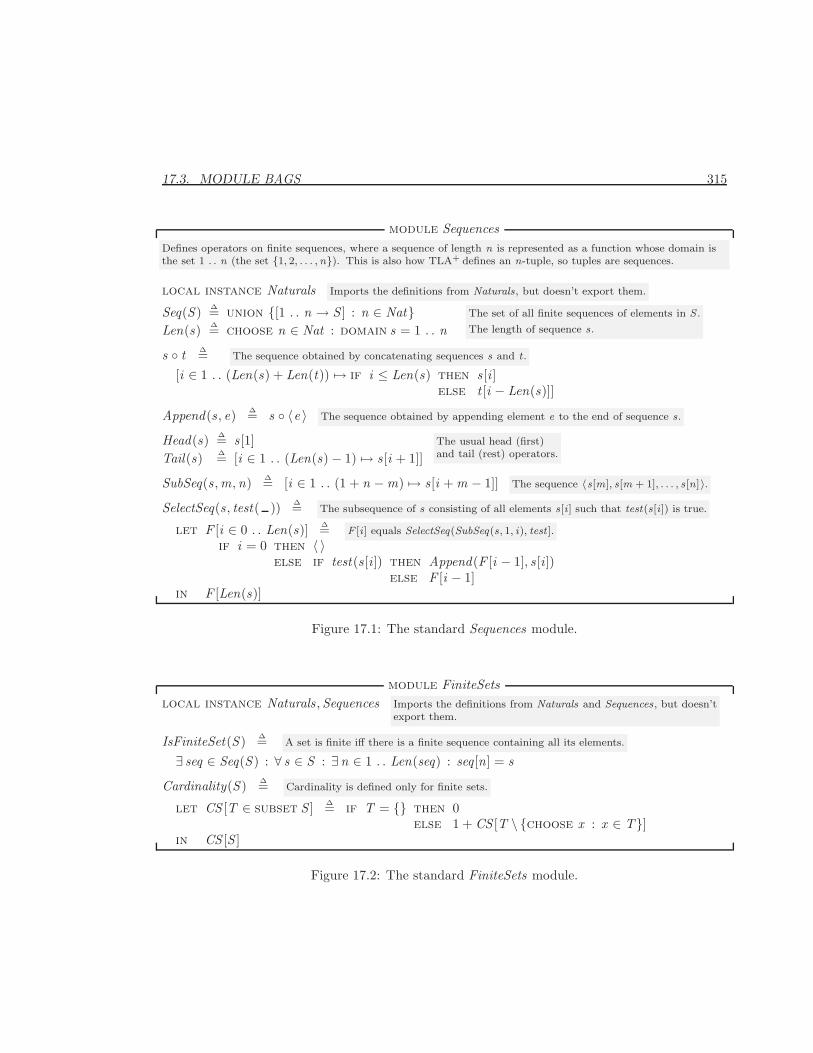
17.3. MODULE BAGS 315
module SequencesDefines operators on finite sequences, where a sequence of length n is represented as a function whose domain isthe set 1 . . n (the set {1, 2, . . . ,n}). This is also how TLA+ defines an n-tuple, so tuples are sequences.
local instance Naturals Imports the definitions from Naturals, but doesn’t export them.
Seq(S ) ∆= union {[1 . . n → S ] : n ∈ Nat} The set of all finite sequences of elements in S .
The length of sequence s.Len(s) ∆= choose n ∈ Nat : domain s = 1 . . n
s ◦ t ∆= The sequence obtained by concatenating sequences s and t .
[i ∈ 1 . . (Len(s) + Len(t)) 7→ if i ≤ Len(s) then s [i ]else t [i − Len(s)]]
Append(s , e) ∆= s ◦ 〈e 〉 The sequence obtained by appending element e to the end of sequence s.
Head(s) ∆= s [1]Tail(s) ∆= [i ∈ 1 . . (Len(s)− 1) 7→ s [i + 1]]
The usual head (first)and tail (rest) operators.
SubSeq(s ,m,n) ∆= [i ∈ 1 . . (1 + n −m) 7→ s [i + m − 1]] The sequence 〈s[m], s[m + 1], . . . , s[n]〉.
SelectSeq(s , test( )) ∆= The subsequence of s consisting of all elements s[i ] such that test(s[i ]) is true.
let F [i ∈ 0 . . Len(s)] ∆= F [i ] equals SelectSeq(SubSeq(s, 1, i), test ].
if i = 0 then 〈 〉else if test(s [i ]) then Append(F [i − 1], s [i ])
else F [i − 1]in F [Len(s)]
Figure 17.1: The standard Sequences module.
module FiniteSetslocal instance Naturals ,Sequences Imports the definitions from Naturals and Sequences, but doesn’t
export them.
IsFiniteSet(S ) ∆= A set is finite iff there is a finite sequence containing all its elements.
∃ seq ∈ Seq(S ) : ∀ s ∈ S : ∃n ∈ 1 . . Len(seq) : seq[n] = s
Cardinality(S ) ∆= Cardinality is defined only for finite sets.
let CS [T ∈ subset S ] ∆= if T = {} then 0else 1 + CS [T \ {choose x : x ∈ T}]
in CS [S ]
Figure 17.2: The standard FiniteSets module.
316 CHAPTER 17. THE STANDARD MODULES
SetToBag(S ) The bag that contains one copy of every element in theset S .
BagIn(e,B) True iff bag B contains at least one copy of e. BagsIn isthe ∈ operator for bags.
EmptyBag The bag containing no elements.
CopiesIn(e,B) The number of copies of e in bag B . If BagIn(e,B) isfalse, then CopiesIn(e,B) = 0.
B1⊕ B2 The union of bags B1 and B2. The operator ⊕ satisfies
CopiesIn(e,B1 ⊕ B2) = CopiesIn(e,B1) + CopiesIn(e,B2)
for any e and any bags B1 and B2.
B1 B2 The bag B1 with the elements of B2 removed—that is,with one copy of an element removed from B1 for eachcopy of the same element in B2. If B2 has at least asmany copies of e as B1, then B1B2 has no copies of e.
BagUnion(S ) The bag union of all elements of the set S of bags. Forexample, BagUnion({B1,B2,B3}) equals B1⊕B2⊕B3.
B1 v B2 True iff, for all e, bag B2 has at least as many copies ofe as bag B1 does. Thus, v is the analog for bags of ⊆.
SubBag(B) The set of all subbags of bag B . SubBag is the bag analogof the subset operator.
BagOfAll(F , B) The bag analog of the construct {F (x ) : x ∈ B}. It isthe bag that contains, for each element e of bag B , onecopy of F (e) for every copy of e in B . This defines a bagiff, for any value v , the set of e in B such that F (e) = vis finite.
BagCardinality(B) If B is a finite bag (one such that BagToSet(B) is afinite set), then this is its cardinality—the total numberof copies of elements in B . Its value is unspecified if Bis not a finite bag.
The module appears in Figure 17.3 on the next page. Note the local definition ofSum, which makes Sum defined within the Bags module but not in any modulethat extends or instantiates it.
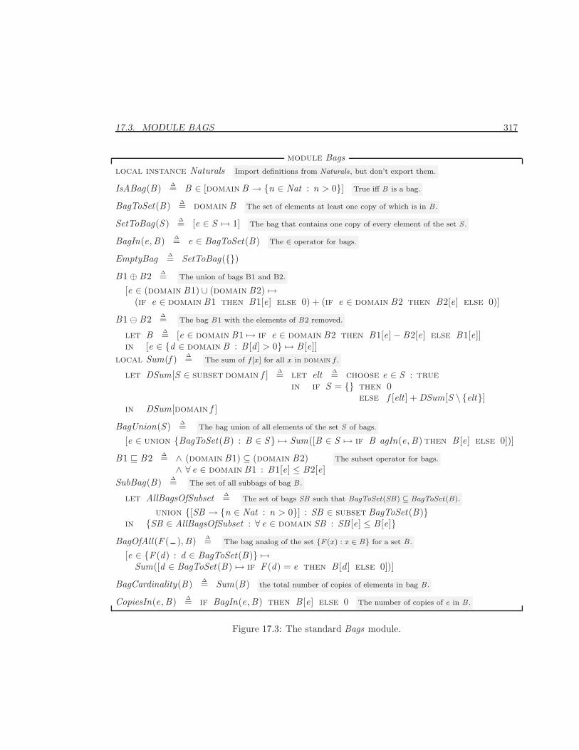
17.3. MODULE BAGS 317
module Bagslocal instance Naturals Import definitions from Naturals, but don’t export them.
IsABag(B) ∆= B ∈ [domain B → {n ∈ Nat : n > 0}] True iff B is a bag.
BagToSet(B) ∆= domain B The set of elements at least one copy of which is in B .
SetToBag(S ) ∆= [e ∈ S 7→ 1] The bag that contains one copy of every element of the set S .
BagIn(e,B) ∆= e ∈ BagToSet(B) The ∈ operator for bags.
EmptyBag ∆= SetToBag({})B1⊕ B2 ∆= The union of bags B1 and B2.
[e ∈ (domain B1) ∪ (domain B2) 7→(if e ∈ domain B1 then B1[e] else 0) + (if e ∈ domain B2 then B2[e] else 0)]
B1 B2 ∆= The bag B1 with the elements of B2 removed.
let B ∆= [e ∈ domain B1 7→ if e ∈ domain B2 then B1[e]− B2[e] else B1[e]]in [e ∈ {d ∈ domain B : B [d ] > 0} 7→ B [e]]
local Sum(f ) ∆= The sum of f [x] for all x in domain f .
let DSum[S ∈ subset domain f ] ∆= let elt ∆= choose e ∈ S : truein if S = {} then 0
else f [elt ] + DSum[S \ {elt}]in DSum[domain f ]
BagUnion(S ) ∆= The bag union of all elements of the set S of bags.
[e ∈ union {BagToSet(B) : B ∈ S} 7→ Sum([B ∈ S 7→ if B agIn(e,B) then B [e] else 0])]
B1 v B2 ∆= ∧ (domain B1) ⊆ (domain B2)∧ ∀ e ∈ domain B1 : B1[e] ≤ B2[e]
The subset operator for bags.
SubBag(B) ∆= The set of all subbags of bag B .
let AllBagsOfSubset ∆= The set of bags SB such that BagToSet(SB) ⊆ BagToSet(B).
union {[SB → {n ∈ Nat : n > 0}] : SB ∈ subset BagToSet(B)}in {SB ∈ AllBagsOfSubset : ∀ e ∈ domain SB : SB [e] ≤ B [e]}
BagOfAll(F ( ),B) ∆= The bag analog of the set {F (x) : x ∈ B} for a set B .
[e ∈ {F (d) : d ∈ BagToSet(B)} 7→Sum([d ∈ BagToSet(B) 7→ if F (d) = e then B [d ] else 0])]
BagCardinality(B) ∆= Sum(B) the total number of copies of elements in bag B .
CopiesIn(e,B) ∆= if BagIn(e,B) then B [e] else 0 The number of copies of e in B .
Figure 17.3: The standard Bags module.
318 CHAPTER 17. THE STANDARD MODULES
17.4 The Numbers Modules
The usual sets of numbers and operators on them are defined in the three mod-ules Naturals , Integers , and Reals . These modules are tricky because theirdefinitions must be consistent. A module M might extend both the Naturalsmodule and another module that extends the Reals module. The module Mthereby obtains two definitions of an operator such as +, one from Naturals andone from Reals . These two definitions of + must be the same. To make them thesame, we have them both come from the definition of + in a module ProtoReals ,which is locally instantiated by both Naturals and Reals .
The Naturals module defines the following operators:
+ ∗ < ≤ Nat ÷ integer division
− binary minus ^ exponentiation > ≥ . . %
Except for ÷, these operators are all either standard or explained in Chapter 2.We define integer division ÷ and modulus % so that for any integer a andpositive integer b:
a % b ∈ 0 . . (b − 1) a = b ∗ (a ÷ b) + (a % b)
The Integers module extends the Naturals module and also defines the set Intof integers and unary minus (−). The Reals module extends Integers and intro-duces the set Real of real numbers and ordinary division (/). In mathematics,(unlike programming languages), integers are real numbers. Hence, Nat is asubset of Int , which is a subset of Real .
The Reals module also defines the special value Infinity. Infinity, whichrepresents a mathematical ∞, satisfies the following two properties:
∀ r ∈ Real : −Infinity < r < Infinity − (−Infinity) = Infinity
The precise details of the number modules are of no practical importance.When writing specifications, you can just assume that the operators they definehave their usual meanings. If you want to prove something about a specification,you can reason about numbers however you want. Tools like model checkersand theorem provers that care about these operators will have their own ways ofhandling them. The modules are given here mainly for completeness. They canalso serve as models if you want to define other basic mathematical structures.However, such definitions are rarely necessary for engineering specifications.
The set Nat of natural numbers, with its zero element and successor functionis defined in the Peano module, which appears in Figure 17.4 on the next page.It simply defines the naturals to be a set satisfying Peano’s axioms [?]. This def-inition is separated into its own module for the following reason. As explained inSection 15.1.9 (page 280) and Section 15.1.10 (page 281), the meanings of tuplesand strings are defined in terms of the natural numbers. The Peano module,
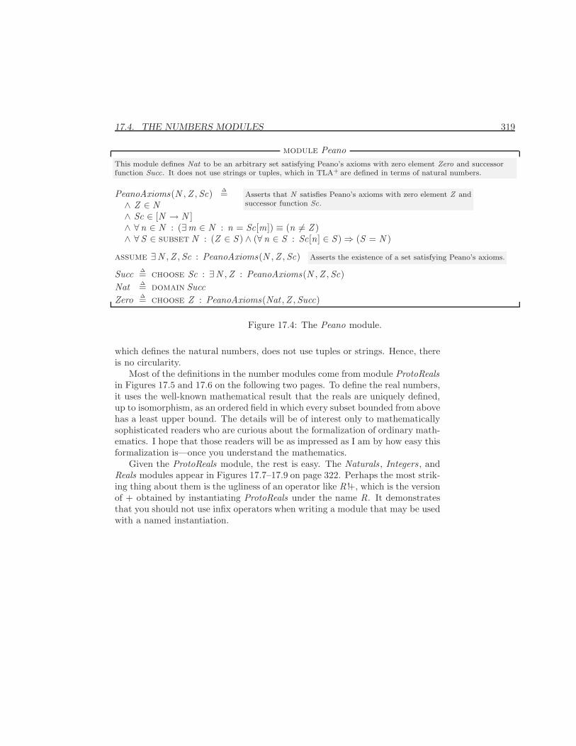
17.4. THE NUMBERS MODULES 319
module PeanoThis module defines Nat to be an arbitrary set satisfying Peano’s axioms with zero element Zero and successorfunction Succ. It does not use strings or tuples, which in TLA+ are defined in terms of natural numbers.
PeanoAxioms(N ,Z ,Sc) ∆= Asserts that N satisfies Peano’s axioms with zero element Z andsuccessor function Sc.∧ Z ∈ N
∧ Sc ∈ [N → N ]∧ ∀n ∈ N : (∃m ∈ N : n = Sc[m]) ≡ (n 6= Z )∧ ∀S ∈ subset N : (Z ∈ S ) ∧ (∀n ∈ S : Sc[n] ∈ S )⇒ (S = N )
assume ∃N ,Z ,Sc : PeanoAxioms(N ,Z ,Sc) Asserts the existence of a set satisfying Peano’s axioms.
Succ ∆= choose Sc : ∃N ,Z : PeanoAxioms(N ,Z ,Sc)Nat ∆= domain SuccZero ∆= choose Z : PeanoAxioms(Nat ,Z ,Succ)
Figure 17.4: The Peano module.
which defines the natural numbers, does not use tuples or strings. Hence, thereis no circularity.
Most of the definitions in the number modules come from module ProtoRealsin Figures 17.5 and 17.6 on the following two pages. To define the real numbers,it uses the well-known mathematical result that the reals are uniquely defined,up to isomorphism, as an ordered field in which every subset bounded from abovehas a least upper bound. The details will be of interest only to mathematicallysophisticated readers who are curious about the formalization of ordinary math-ematics. I hope that those readers will be as impressed as I am by how easy thisformalization is—once you understand the mathematics.
Given the ProtoReals module, the rest is easy. The Naturals , Integers , andReals modules appear in Figures 17.7–17.9 on page 322. Perhaps the most strik-ing thing about them is the ugliness of an operator like R !+, which is the versionof + obtained by instantiating ProtoReals under the name R. It demonstratesthat you should not use infix operators when writing a module that may be usedwith a named instantiation.
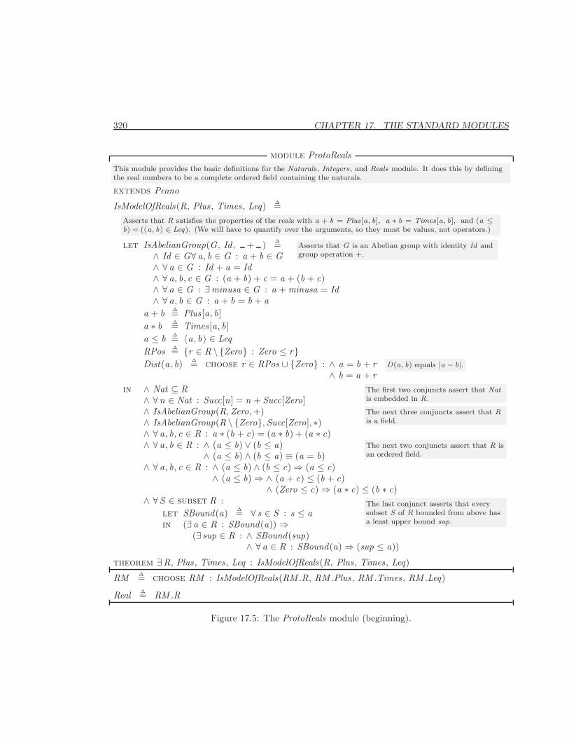
320 CHAPTER 17. THE STANDARD MODULES
module ProtoRealsThis module provides the basic definitions for the Naturals, Integers, and Reals module. It does this by definingthe real numbers to be a complete ordered field containing the naturals.
extends Peano
IsModelOfReals(R, Plus , Times , Leq) ∆=Asserts that R satisfies the properties of the reals with a + b = Plus[a, b], a ∗ b = Times[a, b], and (a ≤b) = (〈a, b 〉 ∈ Leq). (We will have to quantify over the arguments, so they must be values, not operators.)
let IsAbelianGroup(G, Id , + ) ∆= Asserts that G is an Abelian group with identity Id andgroup operation +.∧ Id ∈ G∀ a, b ∈ G : a + b ∈ G
∧ ∀ a ∈ G : Id + a = Id∧ ∀ a, b, c ∈ G : (a + b) + c = a + (b + c)∧ ∀ a ∈ G : ∃minusa ∈ G : a + minusa = Id∧ ∀ a, b ∈ G : a + b = b + a
a + b ∆= Plus [a, b]a ∗ b ∆= Times [a, b]a ≤ b ∆= 〈a, b 〉 ∈ LeqRPos ∆= {r ∈ R \ {Zero} : Zero ≤ r}Dist(a, b) ∆= choose r ∈ RPos ∪ {Zero} : ∧ a = b + r
∧ b = a + rD(a, b) equals |a − b|.
in ∧ Nat ⊆ R∧ ∀n ∈ Nat : Succ[n] = n + Succ[Zero]∧ IsAbelianGroup(R,Zero, +)∧ IsAbelianGroup(R \ {Zero},Succ[Zero], ∗)∧ ∀ a, b, c ∈ R : a ∗ (b + c) = (a ∗ b) + (a ∗ c)∧ ∀ a, b ∈ R : ∧ (a ≤ b) ∨ (b ≤ a)
∧ (a ≤ b) ∧ (b ≤ a) ≡ (a = b)∧ ∀ a, b, c ∈ R : ∧ (a ≤ b) ∧ (b ≤ c)⇒ (a ≤ c)
∧ (a ≤ b)⇒ ∧ (a + c) ≤ (b + c)∧ (Zero ≤ c)⇒ (a ∗ c) ≤ (b ∗ c)
∧ ∀S ∈ subset R :let SBound(a) ∆= ∀ s ∈ S : s ≤ ain (∃ a ∈ R : SBound(a))⇒
(∃ sup ∈ R : ∧ SBound(sup)∧ ∀ a ∈ R : SBound(a)⇒ (sup ≤ a))
The first two conjuncts assert that Natis embedded in R.
The next three conjuncts assert that Ris a field.
The next two conjuncts assert that R isan ordered field.
The last conjunct asserts that everysubset S of R bounded from above hasa least upper bound sup.
theorem ∃R, Plus , Times , Leq : IsModelOfReals(R, Plus , Times , Leq)
RM ∆= choose RM : IsModelOfReals(RM .R, RM .Plus , RM .Times , RM .Leq)
Real ∆= RM .R
Figure 17.5: The ProtoReals module (beginning).
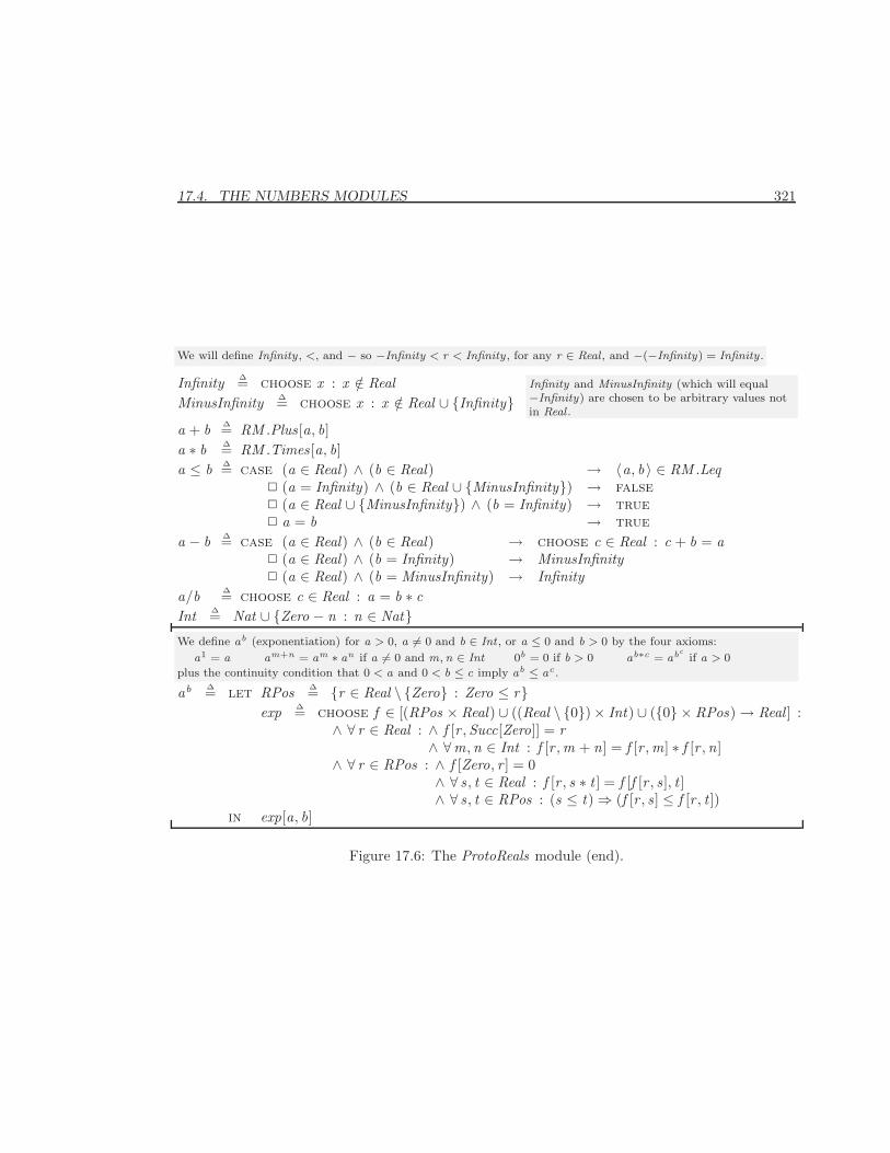
17.4. THE NUMBERS MODULES 321
We will define Infinity , <, and − so −Infinity < r < Infinity , for any r ∈ Real , and −(−Infinity) = Infinity .
Infinity ∆= choose x : x /∈ RealMinusInfinity ∆= choose x : x /∈ Real ∪ {Infinity}
Infinity and MinusInfinity (which will equal−Infinity) are chosen to be arbitrary values notin Real .
a + b ∆= RM .Plus [a, b]a ∗ b ∆= RM .Times [a, b]a ≤ b ∆= case (a ∈ Real) ∧ (b ∈ Real) → 〈a, b 〉 ∈ RM .Leq
2 (a = Infinity) ∧ (b ∈ Real ∪ {MinusInfinity}) → false2 (a ∈ Real ∪ {MinusInfinity}) ∧ (b = Infinity) → true2 a = b → true
a − b ∆= case (a ∈ Real) ∧ (b ∈ Real) → choose c ∈ Real : c + b = a2 (a ∈ Real) ∧ (b = Infinity) → MinusInfinity2 (a ∈ Real) ∧ (b = MinusInfinity) → Infinity
a/b ∆= choose c ∈ Real : a = b ∗ cInt ∆= Nat ∪ {Zero − n : n ∈ Nat}We define ab (exponentiation) for a > 0, a 6= 0 and b ∈ Int , or a ≤ 0 and b > 0 by the four axioms:
a1 = a am+n = am ∗ an if a 6= 0 and m, n ∈ Int 0b = 0 if b > 0 ab∗c = abcif a > 0
plus the continuity condition that 0 < a and 0 < b ≤ c imply ab ≤ ac .
ab ∆= let RPos ∆= {r ∈ Real \ {Zero} : Zero ≤ r}exp ∆= choose f ∈ [(RPos × Real) ∪ ((Real \ {0})× Int) ∪ ({0} × RPos)→ Real ] :
∧ ∀ r ∈ Real : ∧ f [r ,Succ[Zero]] = r∧ ∀m,n ∈ Int : f [r ,m + n] = f [r ,m] ∗ f [r ,n]
∧ ∀ r ∈ RPos : ∧ f [Zero, r ] = 0∧ ∀ s , t ∈ Real : f [r , s ∗ t ] = f [f [r , s ], t ]∧ ∀ s , t ∈ RPos : (s ≤ t)⇒ (f [r , s ] ≤ f [r , t ])
in exp[a, b]
Figure 17.6: The ProtoReals module (end).
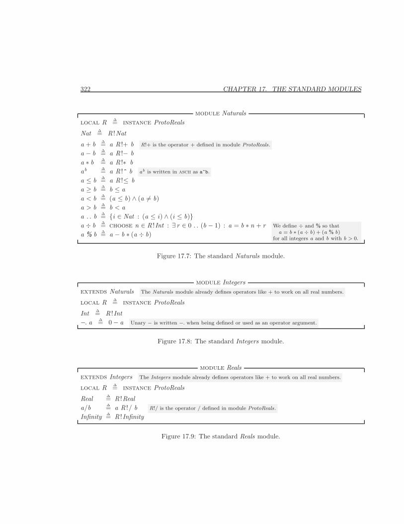
322 CHAPTER 17. THE STANDARD MODULES
module Naturalslocal R ∆= instance ProtoReals
Nat ∆= R !Nat
a + b ∆= a R !+ b R!+ is the operator + defined in module ProtoReals.
a − b ∆= a R !− ba ∗ b ∆= a R !∗ bab ∆= a R !^ b ab is written in ascii as a^b.
a ≤ b ∆= a R !≤ ba ≥ b ∆= b ≤ aa < b ∆= (a ≤ b) ∧ (a 6= b)a > b ∆= b < aa . . b ∆= {i ∈ Nat : (a ≤ i) ∧ (i ≤ b)}a ÷ b ∆= choose n ∈ R !Int : ∃ r ∈ 0 . . (b − 1) : a = b ∗ n + r We define ÷ and % so that
a = b ∗ (a ÷ b) + (a % b)for all integers a and b with b > 0.
a % b ∆= a − b ∗ (a ÷ b)
Figure 17.7: The standard Naturals module.
module Integersextends Naturals The Naturals module already defines operators like + to work on all real numbers.
local R ∆= instance ProtoReals
Int ∆= R !Int−. a ∆= 0− a Unary − is written −. when being defined or used as an operator argument.
Figure 17.8: The standard Integers module.
module Realsextends Integers The Integers module already defines operators like + to work on all real numbers.
local R ∆= instance ProtoReals
Real ∆= R !Reala/b ∆= a R !/ b R!/ is the operator / defined in module ProtoReals.
Infinity ∆= R !Infinity
Figure 17.9: The standard Reals module.

Part V
Appendix
323

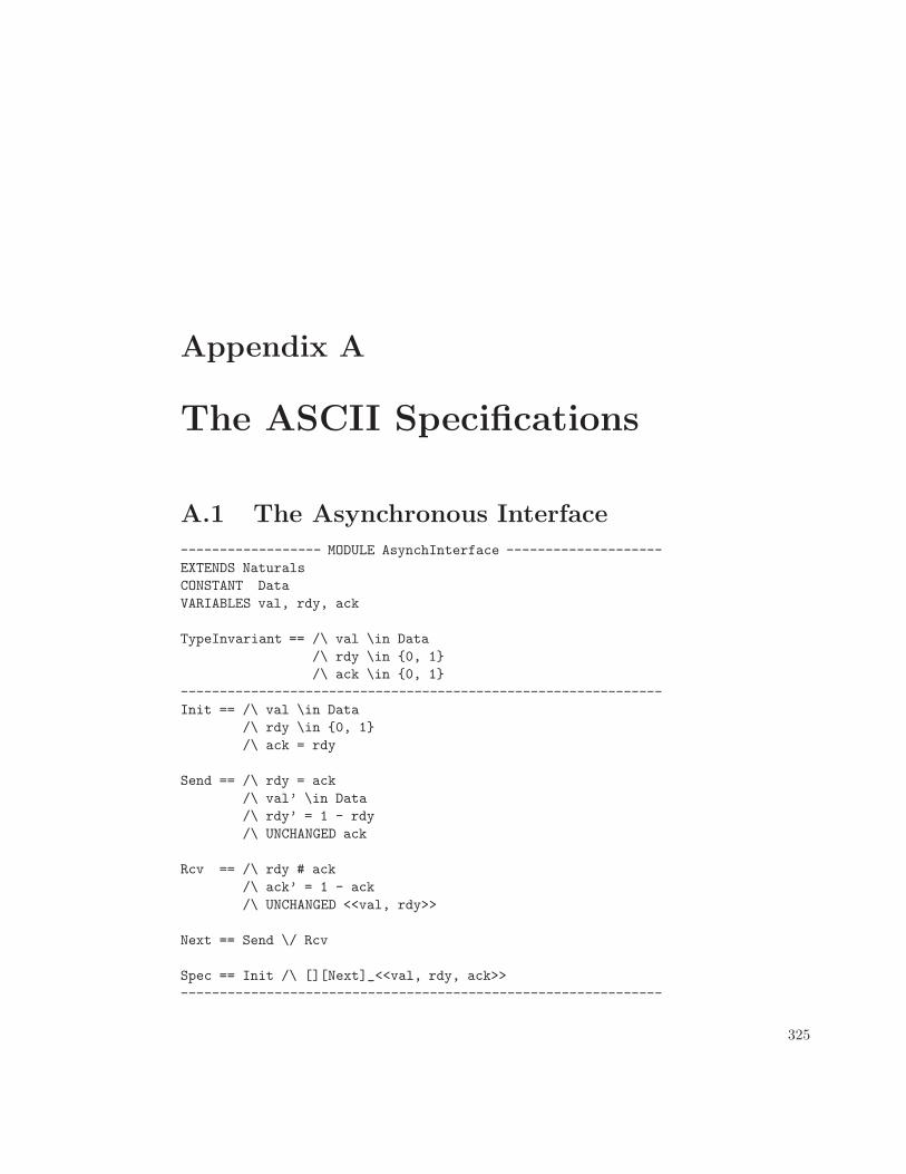
Appendix A
The ASCII Specifications
A.1 The Asynchronous Interface
------------------ MODULE AsynchInterface --------------------EXTENDS NaturalsCONSTANT DataVARIABLES val, rdy, ack
TypeInvariant == /\ val \in Data/\ rdy \in {0, 1}/\ ack \in {0, 1}
--------------------------------------------------------------Init == /\ val \in Data
/\ rdy \in {0, 1}/\ ack = rdy
Send == /\ rdy = ack/\ val’ \in Data/\ rdy’ = 1 - rdy/\ UNCHANGED ack
Rcv == /\ rdy # ack/\ ack’ = 1 - ack/\ UNCHANGED <<val, rdy>>
Next == Send \/ Rcv
Spec == Init /\ [][Next]_<<val, rdy, ack>>--------------------------------------------------------------
325
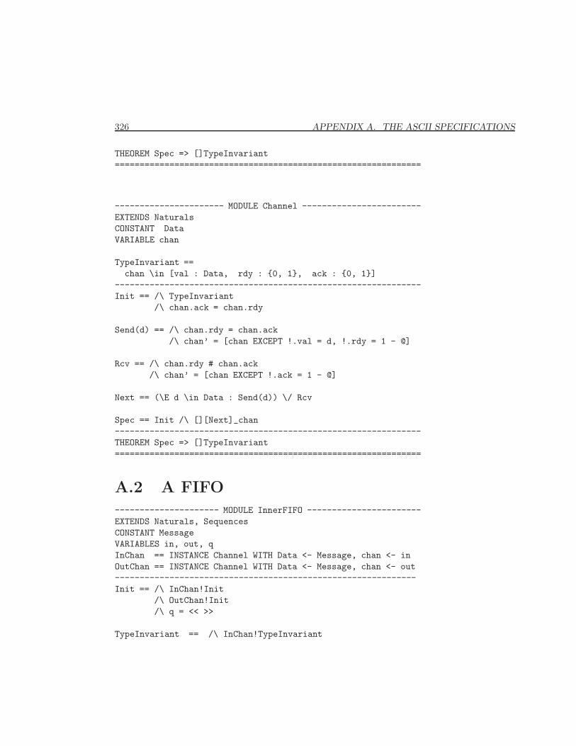
326 APPENDIX A. THE ASCII SPECIFICATIONS
THEOREM Spec => []TypeInvariant==============================================================
---------------------- MODULE Channel ------------------------EXTENDS NaturalsCONSTANT DataVARIABLE chan
TypeInvariant ==chan \in [val : Data, rdy : {0, 1}, ack : {0, 1}]
--------------------------------------------------------------Init == /\ TypeInvariant
/\ chan.ack = chan.rdy
Send(d) == /\ chan.rdy = chan.ack/\ chan’ = [chan EXCEPT !.val = d, !.rdy = 1 - @]
Rcv == /\ chan.rdy # chan.ack/\ chan’ = [chan EXCEPT !.ack = 1 - @]
Next == (\E d \in Data : Send(d)) \/ Rcv
Spec == Init /\ [][Next]_chan--------------------------------------------------------------THEOREM Spec => []TypeInvariant==============================================================
A.2 A FIFO
--------------------- MODULE InnerFIFO -----------------------EXTENDS Naturals, SequencesCONSTANT MessageVARIABLES in, out, qInChan == INSTANCE Channel WITH Data <- Message, chan <- inOutChan == INSTANCE Channel WITH Data <- Message, chan <- out-------------------------------------------------------------Init == /\ InChan!Init
/\ OutChan!Init/\ q = << >>
TypeInvariant == /\ InChan!TypeInvariant
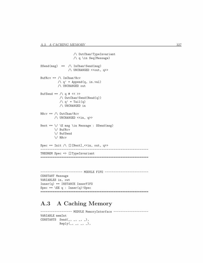
A.3. A CACHING MEMORY 327
/\ OutChan!TypeInvariant/\ q \in Seq(Message)
SSend(msg) == /\ InChan!Send(msg)/\ UNCHANGED <<out, q>>
BufRcv == /\ InChan!Rcv/\ q’ = Append(q, in.val)/\ UNCHANGED out
BufSend == /\ q # << >>/\ OutChan!Send(Head(q))/\ q’ = Tail(q)/\ UNCHANGED in
RRcv == /\ OutChan!Rcv/\ UNCHANGED <<in, q>>
Next == \/ \E msg \in Message : SSend(msg)\/ BufRcv\/ BufSend\/ RRcv
Spec == Init /\ [][Next]_<<in, out, q>>--------------------------------------------------------------THEOREM Spec => []TypeInvariant==============================================================
------------------------ MODULE FIFO -------------------------CONSTANT MessageVARIABLES in, outInner(q) == INSTANCE InnerFIFOSpec == \EE q : Inner(q)!Spec==============================================================
A.3 A Caching Memory
------------------ MODULE MemoryInterface --------------------VARIABLE memIntCONSTANTS Send(_, _, _, _),
Reply(_, _, _, _),
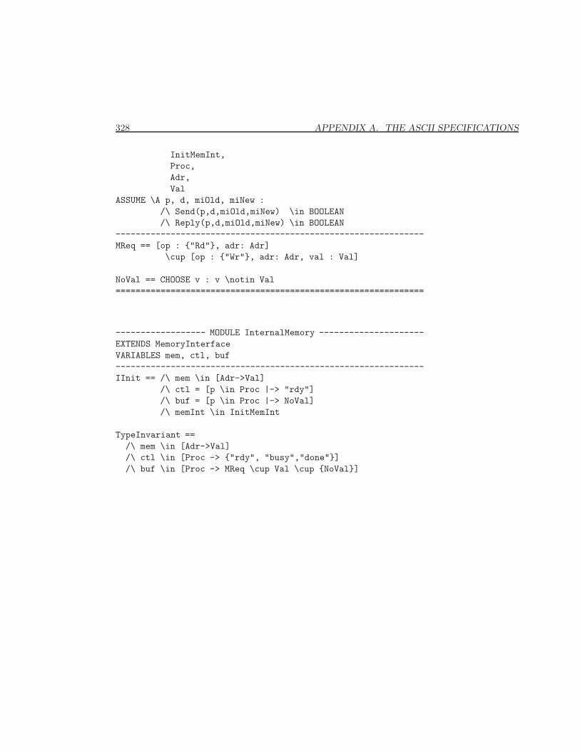
328 APPENDIX A. THE ASCII SPECIFICATIONS
InitMemInt,Proc,Adr,Val
ASSUME \A p, d, miOld, miNew :/\ Send(p,d,miOld,miNew) \in BOOLEAN/\ Reply(p,d,miOld,miNew) \in BOOLEAN
--------------------------------------------------------------MReq == [op : {"Rd"}, adr: Adr]
\cup [op : {"Wr"}, adr: Adr, val : Val]
NoVal == CHOOSE v : v \notin Val==============================================================
------------------ MODULE InternalMemory ---------------------EXTENDS MemoryInterfaceVARIABLES mem, ctl, buf--------------------------------------------------------------IInit == /\ mem \in [Adr->Val]
/\ ctl = [p \in Proc |-> "rdy"]/\ buf = [p \in Proc |-> NoVal]/\ memInt \in InitMemInt
TypeInvariant ==/\ mem \in [Adr->Val]/\ ctl \in [Proc -> {"rdy", "busy","done"}]/\ buf \in [Proc -> MReq \cup Val \cup {NoVal}]
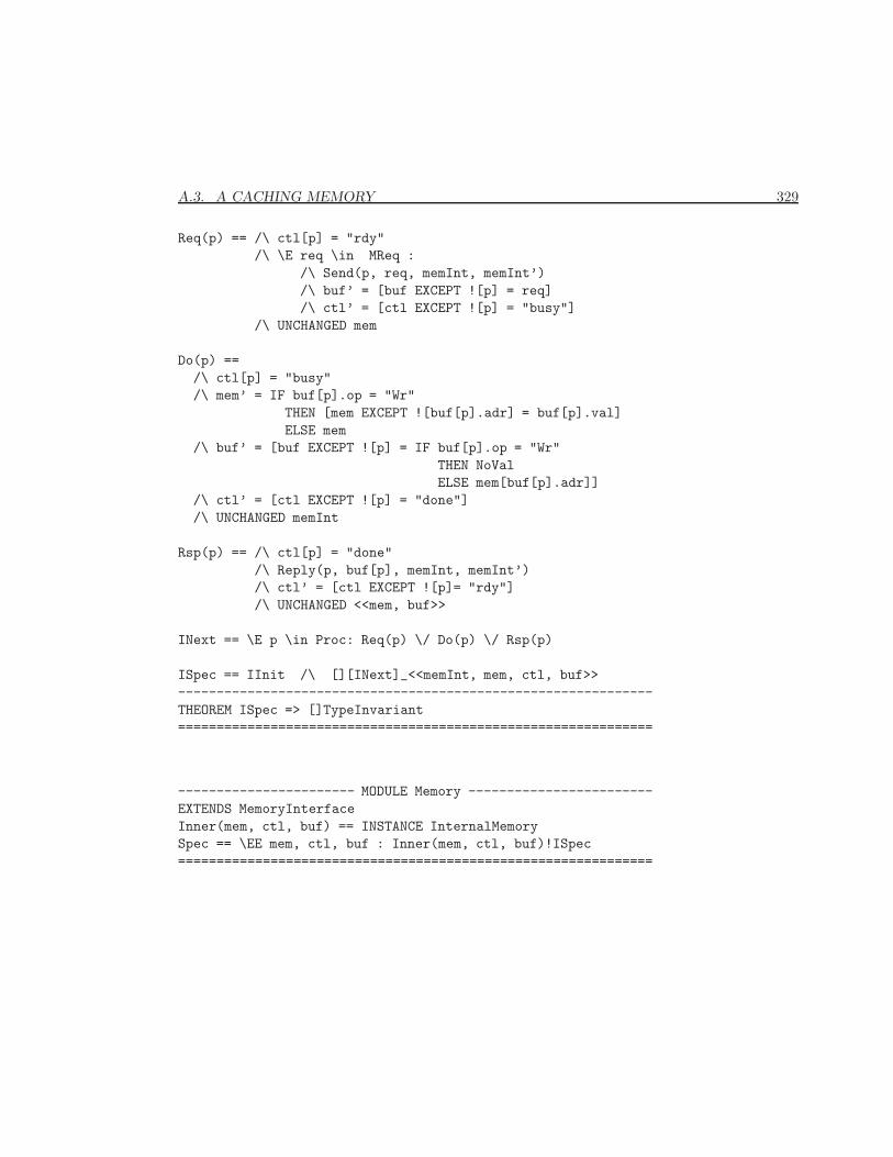
A.3. A CACHING MEMORY 329
Req(p) == /\ ctl[p] = "rdy"/\ \E req \in MReq :
/\ Send(p, req, memInt, memInt’)/\ buf’ = [buf EXCEPT ![p] = req]/\ ctl’ = [ctl EXCEPT ![p] = "busy"]
/\ UNCHANGED mem
Do(p) ==/\ ctl[p] = "busy"/\ mem’ = IF buf[p].op = "Wr"
THEN [mem EXCEPT ![buf[p].adr] = buf[p].val]ELSE mem
/\ buf’ = [buf EXCEPT ![p] = IF buf[p].op = "Wr"THEN NoValELSE mem[buf[p].adr]]
/\ ctl’ = [ctl EXCEPT ![p] = "done"]/\ UNCHANGED memInt
Rsp(p) == /\ ctl[p] = "done"/\ Reply(p, buf[p], memInt, memInt’)/\ ctl’ = [ctl EXCEPT ![p]= "rdy"]/\ UNCHANGED <<mem, buf>>
INext == \E p \in Proc: Req(p) \/ Do(p) \/ Rsp(p)
ISpec == IInit /\ [][INext]_<<memInt, mem, ctl, buf>>--------------------------------------------------------------THEOREM ISpec => []TypeInvariant==============================================================
----------------------- MODULE Memory ------------------------EXTENDS MemoryInterfaceInner(mem, ctl, buf) == INSTANCE InternalMemorySpec == \EE mem, ctl, buf : Inner(mem, ctl, buf)!ISpec==============================================================
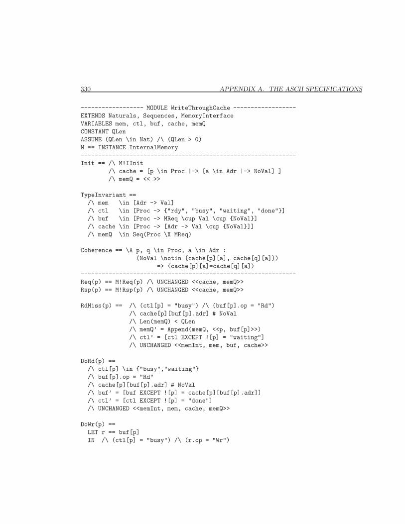
330 APPENDIX A. THE ASCII SPECIFICATIONS
------------------ MODULE WriteThroughCache ------------------EXTENDS Naturals, Sequences, MemoryInterfaceVARIABLES mem, ctl, buf, cache, memQCONSTANT QLenASSUME (QLen \in Nat) /\ (QLen > 0)M == INSTANCE InternalMemory--------------------------------------------------------------Init == /\ M!IInit
/\ cache = [p \in Proc |-> [a \in Adr |-> NoVal] ]/\ memQ = << >>
TypeInvariant ==/\ mem \in [Adr -> Val]/\ ctl \in [Proc -> {"rdy", "busy", "waiting", "done"}]/\ buf \in [Proc -> MReq \cup Val \cup {NoVal}]/\ cache \in [Proc -> [Adr -> Val \cup {NoVal}]]/\ memQ \in Seq(Proc \X MReq)
Coherence == \A p, q \in Proc, a \in Adr :(NoVal \notin {cache[p][a], cache[q][a]})
=> (cache[p][a]=cache[q][a])--------------------------------------------------------------Req(p) == M!Req(p) /\ UNCHANGED <<cache, memQ>>Rsp(p) == M!Rsp(p) /\ UNCHANGED <<cache, memQ>>
RdMiss(p) == /\ (ctl[p] = "busy") /\ (buf[p].op = "Rd")/\ cache[p][buf[p].adr] # NoVal/\ Len(memQ) < QLen/\ memQ’ = Append(memQ, <<p, buf[p]>>)/\ ctl’ = [ctl EXCEPT ![p] = "waiting"]/\ UNCHANGED <<memInt, mem, buf, cache>>
DoRd(p) ==/\ ctl[p] \in {"busy","waiting"}/\ buf[p].op = "Rd"/\ cache[p][buf[p].adr] # NoVal/\ buf’ = [buf EXCEPT ![p] = cache[p][buf[p].adr]]/\ ctl’ = [ctl EXCEPT ![p] = "done"]/\ UNCHANGED <<memInt, mem, cache, memQ>>
DoWr(p) ==LET r == buf[p]IN /\ (ctl[p] = "busy") /\ (r.op = "Wr")
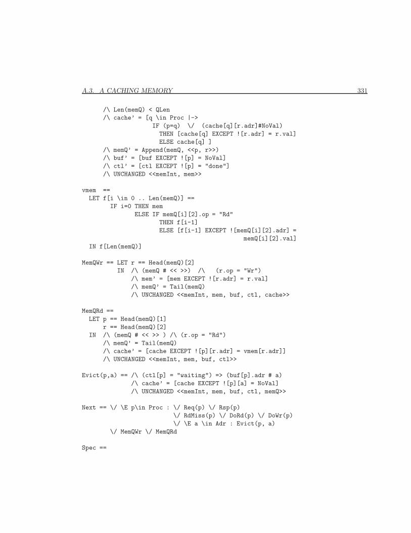
A.3. A CACHING MEMORY 331
/\ Len(memQ) < QLen/\ cache’ = [q \in Proc |->
IF (p=q) \/ (cache[q][r.adr]#NoVal)THEN [cache[q] EXCEPT ![r.adr] = r.val]ELSE cache[q] ]
/\ memQ’ = Append(memQ, <<p, r>>)/\ buf’ = [buf EXCEPT ![p] = NoVal]/\ ctl’ = [ctl EXCEPT ![p] = "done"]/\ UNCHANGED <<memInt, mem>>
vmem ==LET f[i \in 0 .. Len(memQ)] ==
IF i=0 THEN memELSE IF memQ[i][2].op = "Rd"
THEN f[i-1]ELSE [f[i-1] EXCEPT ![memQ[i][2].adr] =
memQ[i][2].val]IN f[Len(memQ)]
MemQWr == LET r == Head(memQ)[2]IN /\ (memQ # << >>) /\ (r.op = "Wr")
/\ mem’ = [mem EXCEPT ![r.adr] = r.val]/\ memQ’ = Tail(memQ)/\ UNCHANGED <<memInt, mem, buf, ctl, cache>>
MemQRd ==LET p == Head(memQ)[1]
r == Head(memQ)[2]IN /\ (memQ # << >> ) /\ (r.op = "Rd")
/\ memQ’ = Tail(memQ)/\ cache’ = [cache EXCEPT ![p][r.adr] = vmem[r.adr]]/\ UNCHANGED <<memInt, mem, buf, ctl>>
Evict(p,a) == /\ (ctl[p] = "waiting") => (buf[p].adr # a)/\ cache’ = [cache EXCEPT ![p][a] = NoVal]/\ UNCHANGED <<memInt, mem, buf, ctl, memQ>>
Next == \/ \E p\in Proc : \/ Req(p) \/ Rsp(p)\/ RdMiss(p) \/ DoRd(p) \/ DoWr(p)\/ \E a \in Adr : Evict(p, a)
\/ MemQWr \/ MemQRd
Spec ==
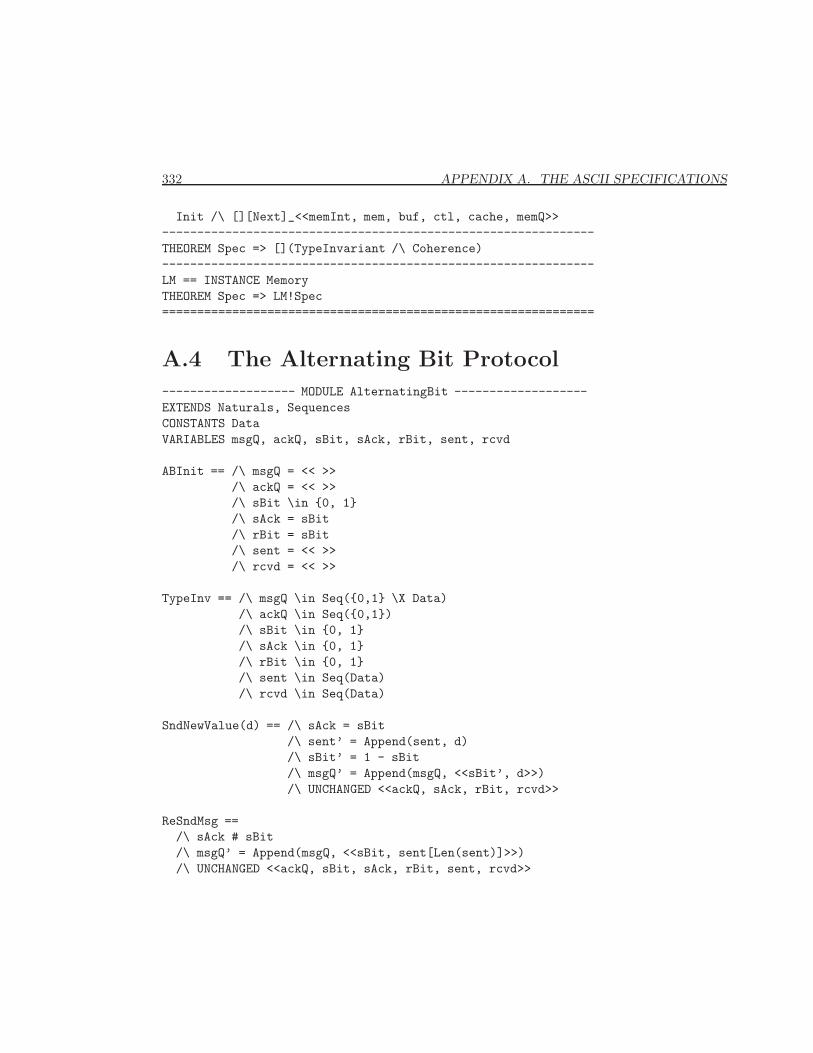
332 APPENDIX A. THE ASCII SPECIFICATIONS
Init /\ [][Next]_<<memInt, mem, buf, ctl, cache, memQ>>--------------------------------------------------------------THEOREM Spec => [](TypeInvariant /\ Coherence)--------------------------------------------------------------LM == INSTANCE MemoryTHEOREM Spec => LM!Spec==============================================================
A.4 The Alternating Bit Protocol
------------------- MODULE AlternatingBit -------------------EXTENDS Naturals, SequencesCONSTANTS DataVARIABLES msgQ, ackQ, sBit, sAck, rBit, sent, rcvd
ABInit == /\ msgQ = << >>/\ ackQ = << >>/\ sBit \in {0, 1}/\ sAck = sBit/\ rBit = sBit/\ sent = << >>/\ rcvd = << >>
TypeInv == /\ msgQ \in Seq({0,1} \X Data)/\ ackQ \in Seq({0,1})/\ sBit \in {0, 1}/\ sAck \in {0, 1}/\ rBit \in {0, 1}/\ sent \in Seq(Data)/\ rcvd \in Seq(Data)
SndNewValue(d) == /\ sAck = sBit/\ sent’ = Append(sent, d)/\ sBit’ = 1 - sBit/\ msgQ’ = Append(msgQ, <<sBit’, d>>)/\ UNCHANGED <<ackQ, sAck, rBit, rcvd>>
ReSndMsg ==/\ sAck # sBit/\ msgQ’ = Append(msgQ, <<sBit, sent[Len(sent)]>>)/\ UNCHANGED <<ackQ, sBit, sAck, rBit, sent, rcvd>>
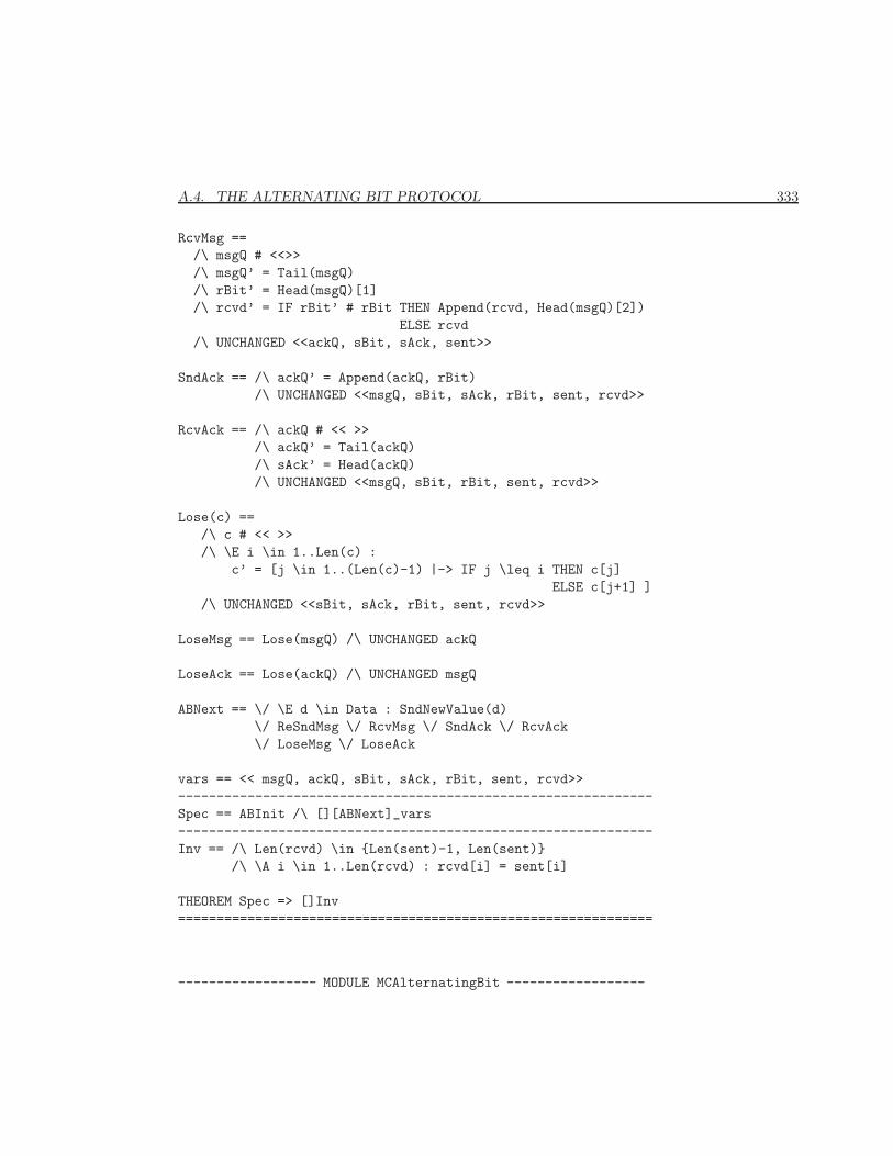
A.4. THE ALTERNATING BIT PROTOCOL 333
RcvMsg ==/\ msgQ # <<>>/\ msgQ’ = Tail(msgQ)/\ rBit’ = Head(msgQ)[1]/\ rcvd’ = IF rBit’ # rBit THEN Append(rcvd, Head(msgQ)[2])
ELSE rcvd/\ UNCHANGED <<ackQ, sBit, sAck, sent>>
SndAck == /\ ackQ’ = Append(ackQ, rBit)/\ UNCHANGED <<msgQ, sBit, sAck, rBit, sent, rcvd>>
RcvAck == /\ ackQ # << >>/\ ackQ’ = Tail(ackQ)/\ sAck’ = Head(ackQ)/\ UNCHANGED <<msgQ, sBit, rBit, sent, rcvd>>
Lose(c) ==/\ c # << >>/\ \E i \in 1..Len(c) :
c’ = [j \in 1..(Len(c)-1) |-> IF j \leq i THEN c[j]ELSE c[j+1] ]
/\ UNCHANGED <<sBit, sAck, rBit, sent, rcvd>>
LoseMsg == Lose(msgQ) /\ UNCHANGED ackQ
LoseAck == Lose(ackQ) /\ UNCHANGED msgQ
ABNext == \/ \E d \in Data : SndNewValue(d)\/ ReSndMsg \/ RcvMsg \/ SndAck \/ RcvAck\/ LoseMsg \/ LoseAck
vars == << msgQ, ackQ, sBit, sAck, rBit, sent, rcvd>>--------------------------------------------------------------Spec == ABInit /\ [][ABNext]_vars--------------------------------------------------------------Inv == /\ Len(rcvd) \in {Len(sent)-1, Len(sent)}
/\ \A i \in 1..Len(rcvd) : rcvd[i] = sent[i]
THEOREM Spec => []Inv==============================================================
------------------ MODULE MCAlternatingBit ------------------
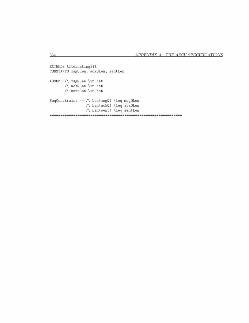
334 APPENDIX A. THE ASCII SPECIFICATIONS
EXTENDS AlternatingBitCONSTANTS msgQLen, ackQLen, sentLen
ASSUME /\ msgQLen \in Nat/\ ackQLen \in Nat/\ sentLen \in Nat
SeqConstraint == /\ Len(msgQ) \leq msgQLen/\ Len(ackQ) \leq ackQLen/\ Len(sent) \leq sentLen
==============================================================

Bibliography
[1] Donald E. Knuth. The TEXbook. Addison-Wesley, Reading, Massachusetts,1994.
[2] Leslie Lamport. The temporal logic of actions. ACM Transactions on Pro-gramming Languages and Systems, 16(3):872–923, May 1994.
[3] A. C. Leisenring. Mathematical Logic and Hilbert’s ε-Symbol. Gordon andBreach, New York, 1969.
335