Embed Size (px)
Citation preview
Master’s Thesis
Specification and Verification ofConvergent Replicated Data Types
Peter [email protected]
November 2013
Department of Computer Science,University of Kaiserslautern,
D 67653 Kaiserslautern,Germany
Supervisors:
Prof. Dr. Arnd Poetzsch-HeffterDr. Annette Bieniusa


Ich versichere hiermit, dass ich die vorliegende Masterarbeit mit dem Thema “Spec-ification and Verification of Convergent Replicated Data Types” selbstständig verfasstund keine anderen als die angegebenen Hilfsmittel benutzt habe. Die Stellen, die an-deren Werken dem Wortlaut oder dem Sinn nach entnommen wurden, habe ich durchdie Angabe der Quelle, auch der benutzten Sekundärliteratur, als Entlehnung kenntlichgemacht.
(Ort, Datum) (Unterschrift)

Abstract Conflict Free Replicated Data Types (CRDTs) can be used as basic buildingblocks for storing and managing data in a distributed system. They provide high avail-ability and performance, and they guarantee that conflicts are resolved in a well definedway. In this master’s thesis, techniques for verifying these data types with the inter-active theorem prover Isabelle/HOL are presented. The verification covers convergenceproperties, as well as behavioral specifications. For this task, a basic framework for theverification of CRDTs has been developed and several known CRDTs from the literaturehave been verified using the framework. The result are machine checked proofs for thecorrectness of the CRDTs, which rely on only a small set of unchecked assumptions,which are captured in a simple system model.
Zusammenfassung Conflict Free Replicated Data Types (CRDTs) können als grundle-gende Bausteine für das Speichern und Verwalten von Daten in verteilten Systemen ver-wendet werden. Sie bieten eine hohe Verfügbarkeit und Performanz und sie garantieren,dass Konflikte auf eine wohldefinierte Art und Weise aufgelöst werden. In dieser Arbeitwerden Techniken zum verifizieren dieser Datentypen mit dem interaktivem Theorem-Beweiser Isabelle/HOL vorgestellt. Die Verifikation umfasst sowohl Konvergenz-Eigen-schaften, als auch Spezifikationen, die das Verhalten betreffen. Dafür wurde ein grundle-gendes System für das verifizieren von CRDTs entwickelt und mehrere bekannte CRDTsaus der Literatur wurden damit verifiziert. Das Ergebnis sind vom Computer geprüfteBeweise für die Korrektheit dieser CRDTs, die nur von einer kleinen Menge von nichtgeprüften Annahmen ausgehen, welche in einem einfachen System-Modell zusammenge-fasst sind.

Contents1. Introduction 1
2. Conflict-Free Replicated Data Types 32.1. Operation Based CRDTs . . . . . . . . . . . . . . . . . . . . . . . . . . . . 3
2.1.1. Example: Counter . . . . . . . . . . . . . . . . . . . . . . . . . . . 32.1.2. Example: U-Set . . . . . . . . . . . . . . . . . . . . . . . . . . . . 4
2.2. State Based CRDTs . . . . . . . . . . . . . . . . . . . . . . . . . . . . . . 42.2.1. Example: Counter . . . . . . . . . . . . . . . . . . . . . . . . . . . 52.2.2. Example: Two-Phase-Set . . . . . . . . . . . . . . . . . . . . . . . 52.2.3. Example: Observed-Remove-Set . . . . . . . . . . . . . . . . . . . 6
3. System Model for State Based Data Types 93.1. Overview . . . . . . . . . . . . . . . . . . . . . . . . . . . . . . . . . . . . 93.2. Replicas and Version Vectors . . . . . . . . . . . . . . . . . . . . . . . . . 103.3. Data type record . . . . . . . . . . . . . . . . . . . . . . . . . . . . . . . . 113.4. Traces and Actions . . . . . . . . . . . . . . . . . . . . . . . . . . . . . . . 143.5. System State . . . . . . . . . . . . . . . . . . . . . . . . . . . . . . . . . . 153.6. Operational Semantics . . . . . . . . . . . . . . . . . . . . . . . . . . . . . 16
4. Consistency 194.1. Eventual Consistency . . . . . . . . . . . . . . . . . . . . . . . . . . . . . . 194.2. A sufficient condition for Convergence . . . . . . . . . . . . . . . . . . . . 20
5. Specification of CRDTs 275.1. Separated sequential and concurrent specifications . . . . . . . . . . . . . 27
5.1.1. Principle of permutation equivalence . . . . . . . . . . . . . . . . . 285.1.2. Example: Counter . . . . . . . . . . . . . . . . . . . . . . . . . . . 285.1.3. Example: Observed-Remove Set . . . . . . . . . . . . . . . . . . . 295.1.4. Discussion . . . . . . . . . . . . . . . . . . . . . . . . . . . . . . . . 30
5.2. Explicit Specification of Merge . . . . . . . . . . . . . . . . . . . . . . . . 305.2.1. Discussion . . . . . . . . . . . . . . . . . . . . . . . . . . . . . . . . 32
5.3. Specification based on Update History . . . . . . . . . . . . . . . . . . . . 335.3.1. Discussion . . . . . . . . . . . . . . . . . . . . . . . . . . . . . . . . 345.3.2. Realization in Isabelle . . . . . . . . . . . . . . . . . . . . . . . . . 34
6. Verifying CRDT behavior 376.1. Valid update histories . . . . . . . . . . . . . . . . . . . . . . . . . . . . . 406.2. Consistent update histories . . . . . . . . . . . . . . . . . . . . . . . . . . 406.3. Verification by showing equivalence . . . . . . . . . . . . . . . . . . . . . . 40
7. Case Studies 457.1. Increment-Only Counter . . . . . . . . . . . . . . . . . . . . . . . . . . . . 457.2. PN-Counter . . . . . . . . . . . . . . . . . . . . . . . . . . . . . . . . . . . 47
7.3. Grow-Set . . . . . . . . . . . . . . . . . . . . . . . . . . . . . . . . . . . . 497.4. Two-Phase-Set . . . . . . . . . . . . . . . . . . . . . . . . . . . . . . . . . 507.5. Observed-Remove-Set . . . . . . . . . . . . . . . . . . . . . . . . . . . . . 52
7.5.1. Simplified Implementation . . . . . . . . . . . . . . . . . . . . . . . 527.5.2. Original Implementation . . . . . . . . . . . . . . . . . . . . . . . . 557.5.3. Optimized Implementation . . . . . . . . . . . . . . . . . . . . . . 59
7.6. Multi-Value-Register . . . . . . . . . . . . . . . . . . . . . . . . . . . . . . 657.6.1. Simple Implementation . . . . . . . . . . . . . . . . . . . . . . . . 657.6.2. Optimized Implementation . . . . . . . . . . . . . . . . . . . . . . 65
8. Related work 71
9. Conclusion and future work 73
Appendices 79
A. Isabelle theories 79
1. Introduction
For many distributed systems, there is a big challenge in managing data. Using a singlenode to store data is often not a feasible option. There are different reasons for this.Some systems require a higher throughput for writing and reading data, than what canbe provided by a single node. Other systems require a high availability, which can onlybe provided by several nodes without a single point of failure. Then there are systemswhich serve clients from different regions in the world and want to avoid the delay ofmessages sent around half the globe. So these systems need nodes located at differentplaces in the world. Finally there are systems where nodes are not always connected. Forexample mobile phones and tablets are not always connected to the Internet and thusneed a local data store on the device, which is only synchronized with a more centraldata store when a connection is available.Classical relational, transactional databases like Microsoft SQL Server, Oracle, or
IBM DB2 try to keep the data stores on different nodes (also called replicas) consistentall the time. But requiring strong consistency has a negative effect on the availabilityand delay of the data store operations. Some newer databases like Riak or Cassandraprovide weaker consistency guarantees and therefore can achieve better availability andperformance. These kind of databases are called eventual consistent as opposed tostrongly consistent. Such databases can often process an operation locally and thensynchronize the changes between the data stores asynchronous to the operation.For many use cases this implies that there can be conflicting updates in distinct
data stores. In such a case the conflict can only be detected after the operation wascompleted, and it has to be resolved either by the database itself or by the application.Letting the application handle conflicts increases the complexity of the application, theprobability of loosing data due to programming errors, and it requires that the databasestores all necessary information about conflicts until they are resolved by the application.Therefore developers usually want the database to handle conflicts by itself according tosome reasonable rules.Unfortunately there is no universal rule to resolve conflicts, as it always depends on
the application. As an example consider an integer variable which is changed from 42to 43 on one replica and changed from 42 to 46 on an other replica. Now there arethe two conflicting values 43 and 46. If the application’s intend was counting, then itwould make sense to resolve the conflict by setting the variable to 47 as this includesthe one new element counted at the first replica and the four new elements counted atthe second replica. However, if the application’s intend was to set the variable to someabsolute value, it might make more sense to resolve the conflict by keeping both valuesor by taking an aggregate function like the maximum of the values.Behaviors like the counter are required in more than one application, so it makes
sense to put this behavior in a reusable data type. Convergent Replicated Data Types(CRDTs) are such data types. They are similar to data types for sequential programssuch as lists, sets, or maps, but they are replicated across multiple nodes. Operations canbe performed on only a single replica and updates are communicated to other replicas
1
at some later time. A common property of all CRDTs is, that they converge, so iftwo replicas have seen the same set of updates they are guaranteed to be in the samestate. This guarantee is also preserved, when replicas are not synchronized for a longerperiod of time and therefore CRDTs are a good approach to address the afore mentionedaspects, namely throughput, availability, delay, and connectivity.When CRDTs are used as data storage of an application, it is essential that the
CRDT implementations behave as intended by the application programmer. Thereforeit is necessary to have a precise specification of how the CRDT behaves and it must beverified that the implementation is a correct implementation of the specification.Testing is one option to check if an implementation behaves as intended, but it is hard
to test all relevant cases. This is especially hard in a concurrent environment, whereeven more different executions are possible for a given number of operations. If a bugis not detected in testing, it is likely that it only occurs in certain corner cases. Thiscan lead to bugs in an application, which are hard to find and hard to debug. Sinceconcurrent applications are usually highly nondeterministic, it can be hard to reproducea bug which only happens in certain cases and it could take some time to detect theproblem. Until the problem is detected, a lot of important data could be lost. BecauseCRDTs can be used in a lot of applications, there would probably be more than oneapplication affected by a bug in a CRDT application. Therefore it is important to besure, that implementations are correct. As testing cannot guarantee correctness, it isnecessary to use static verification. If the static verification is checked by a tool, one canbe sure that an implementation behaves as specified.Verified, formal specifications of CRDTs are also necessary for verifying applications,
which use CRDTs. It is not realistic to verify a whole application directly. Insteadlibraries, and CRDTs can be seen as a library, have to provide a well defined interfacewith a specification, on which higher level proofs can be based.This master’s thesis presents a framework for specifying and verifying CRDTs with
the interactive theorem prover Isabelle/HOL[10]. Different approaches for specifying thebehavior of CRDTs are discussed and the specification and verification techniques areapplied to several CRDT implementations found in the literature.The remainder of this thesis is structured as follows. Section 2 gives a short introduc-
tion to CRDTs and presents state-based and operation-based types. The later chapteronly consider state-based types. Section 3 presents the underlying system model forthis work. Section 4 defines general consistency and convergence properties of CRDTsand the theory required to verify convergence of a implementation. Section 5 discussesdifferent approaches for specifying CRDTs and presents the formalization of the usedspecification technique in Isabelle. Section 6 presents the techniques used for verifyingthat an implementation satisfies its specification. Then section 7 applies the previouslyintroduced techniques to case studies, which are CRDT implementations from the liter-ature.
2
2. Conflict-Free Replicated Data Types
The general idea of Conflict-Free Replicated Data Types (CRDTs) is, that they form areusable component for storing data in a distributed system. A CRDT object is usuallyreplicated onto several nodes in the system and has to include functionality for keepingthe different replicas synchronized. The interface of a CRDT consists of several methodsfor updating and querying the state of the data type. These methods can always beexecuted locally on a single replica. The synchronization with other replicas can happenat a later point in time. [12]The synchronization also is done in a single message, so updates are visible after a sin-
gle message is exchanged. The synchronization does not depend on consensus protocolslike Paxos, or on locking mechanisms, and therefore synchronization is relatively fast.There are two different kind of CRDTs: operation based types and state based types.
The two types differ in the mechanism used for synchronization. Both types have incommon, that they provide a number of update- and query-operations and that a singleinstance of a CRDT consists of several replicas. Every replica has a local state whichis called the payload of the object. There is no global state or central authority in aCRDT instance.
2.1. Operation Based CRDTs
Operation based CRDTs are also called Commutative Replicated Data Types (Cm-RDTs).Operation based CRDTs synchronize on each operation. When an update-method
is executed, the local replica first calculates a so called downstream effect. The down-stream effect is basically a function f : Pl → Pl where Pl is the type of the CRDT’spayload. This function is then used to update the payload of every replica in the system.The local payload is updated immediately and the payload at other replicas is updatedasynchronously.All generated downstream effects are expected to commute. So, if f and g are down-
stream effects, then it should hold that f(g(pl)) = g(f(pl)) for all possible payloadspl.Therefore the underlying network protocol is not required to deliver the downstream
effects in a certain order. However is must be ensured, that each downstream ef-fect is executed exactly once, as downstream effects are not necessary idempotent (i.e.f(f(pl)) = f(pl) does not hold in general).
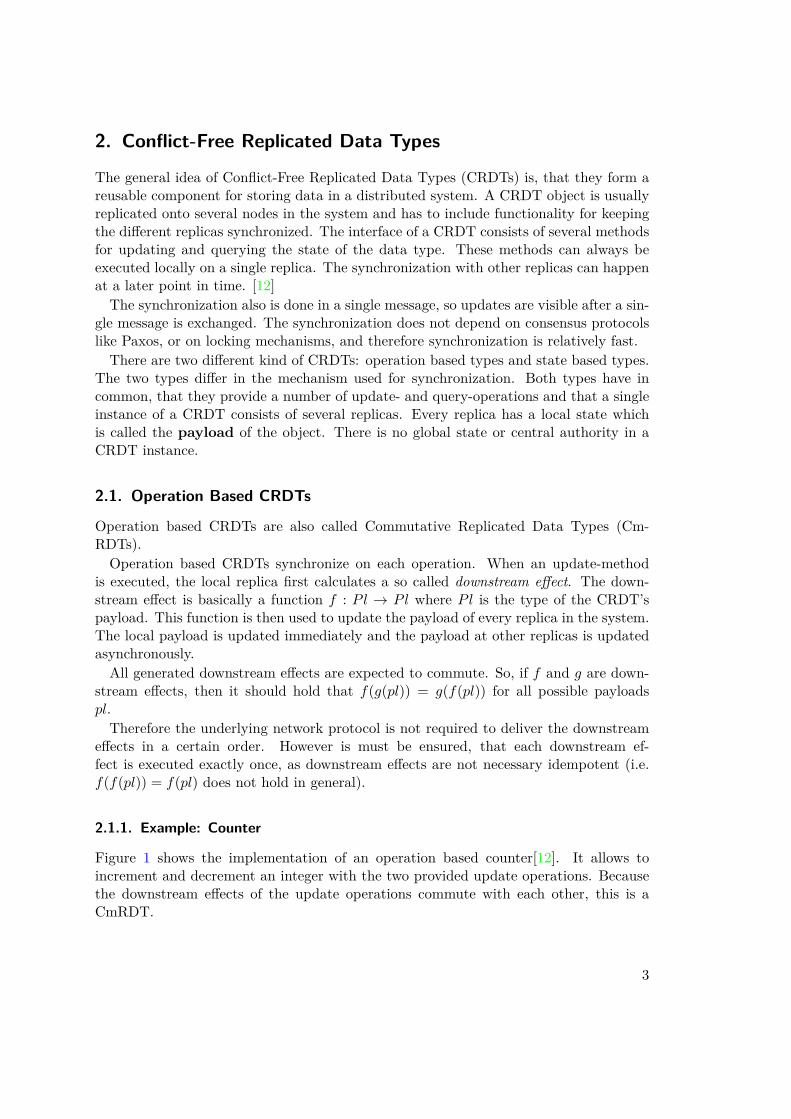
2.1.1. Example: Counter
Figure 1 shows the implementation of an operation based counter[12]. It allows toincrement and decrement an integer with the two provided update operations. Becausethe downstream effects of the update operations commute with each other, this is aCmRDT.
3
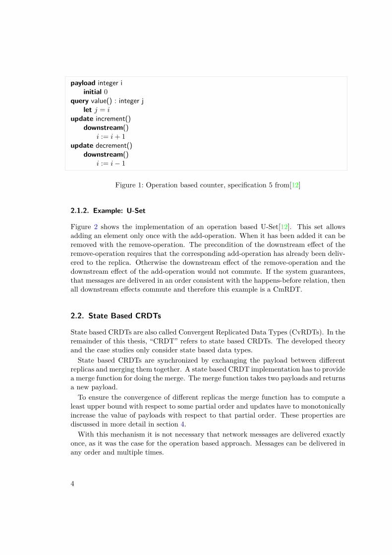
payload integer iinitial 0
query value() : integer jlet j = i
update increment()downstream()
i := i+ 1update decrement()
downstream()i := i− 1
Figure 1: Operation based counter, specification 5 from[12]
2.1.2. Example: U-Set
Figure 2 shows the implementation of an operation based U-Set[12]. This set allowsadding an element only once with the add-operation. When it has been added it can beremoved with the remove-operation. The precondition of the downstream effect of theremove-operation requires that the corresponding add-operation has already been deliv-ered to the replica. Otherwise the downstream effect of the remove-operation and thedownstream effect of the add-operation would not commute. If the system guarantees,that messages are delivered in an order consistent with the happens-before relation, thenall downstream effects commute and therefore this example is a CmRDT.
2.2. State Based CRDTs
State based CRDTs are also called Convergent Replicated Data Types (CvRDTs). In theremainder of this thesis, “CRDT” refers to state based CRDTs. The developed theoryand the case studies only consider state based data types.State based CRDTs are synchronized by exchanging the payload between different
replicas and merging them together. A state based CRDT implementation has to providea merge function for doing the merge. The merge function takes two payloads and returnsa new payload.To ensure the convergence of different replicas the merge function has to compute a
least upper bound with respect to some partial order and updates have to monotonicallyincrease the value of payloads with respect to that partial order. These properties arediscussed in more detail in section 4.With this mechanism it is not necessary that network messages are delivered exactly
once, as it was the case for the operation based approach. Messages can be delivered inany order and multiple times.
4
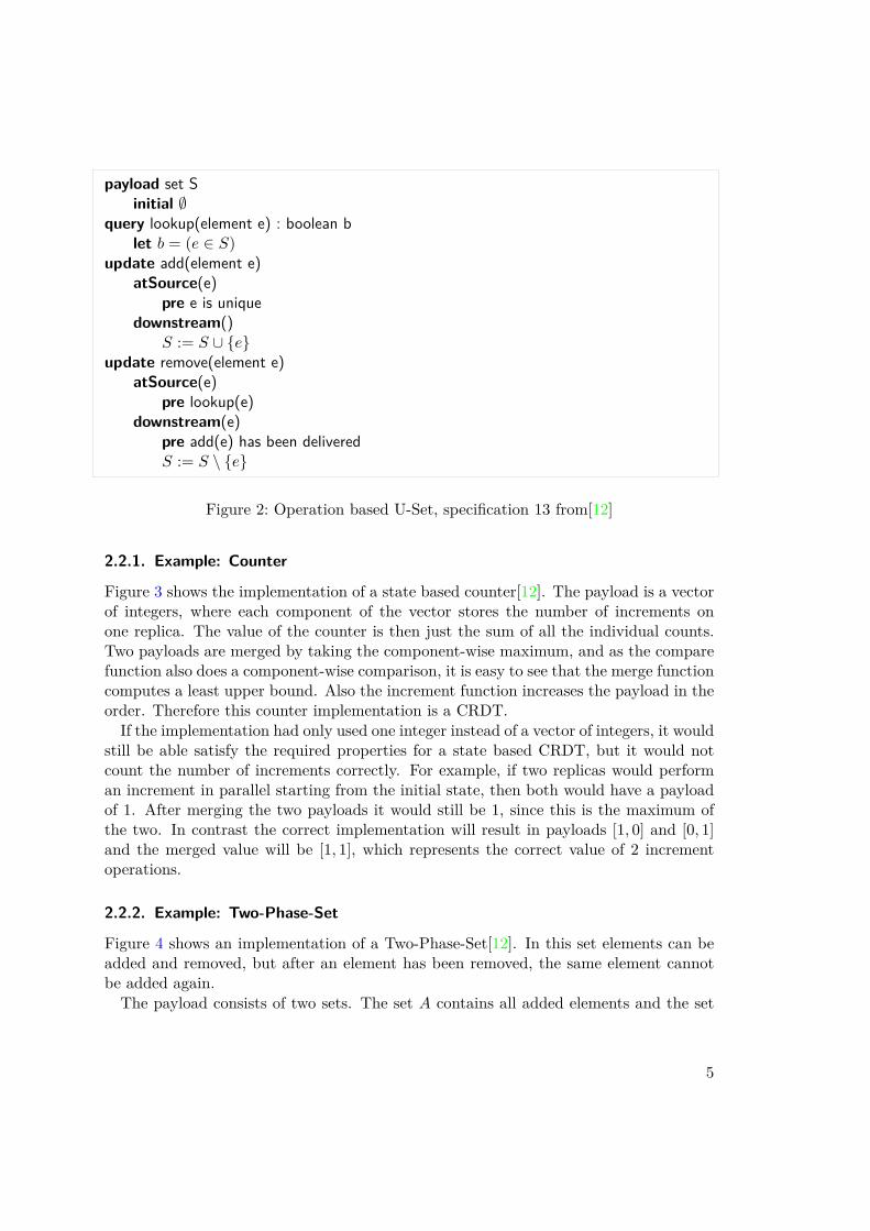
payload set Sinitial ∅
query lookup(element e) : boolean blet b = (e ∈ S)
update add(element e)atSource(e)
pre e is uniquedownstream()
S := S ∪ {e}update remove(element e)
atSource(e)pre lookup(e)
downstream(e)pre add(e) has been deliveredS := S \ {e}
Figure 2: Operation based U-Set, specification 13 from[12]
2.2.1. Example: Counter
Figure 3 shows the implementation of a state based counter[12]. The payload is a vectorof integers, where each component of the vector stores the number of increments onone replica. The value of the counter is then just the sum of all the individual counts.Two payloads are merged by taking the component-wise maximum, and as the comparefunction also does a component-wise comparison, it is easy to see that the merge functioncomputes a least upper bound. Also the increment function increases the payload in theorder. Therefore this counter implementation is a CRDT.If the implementation had only used one integer instead of a vector of integers, it would
still be able satisfy the required properties for a state based CRDT, but it would notcount the number of increments correctly. For example, if two replicas would performan increment in parallel starting from the initial state, then both would have a payloadof 1. After merging the two payloads it would still be 1, since this is the maximum ofthe two. In contrast the correct implementation will result in payloads [1, 0] and [0, 1]and the merged value will be [1, 1], which represents the correct value of 2 incrementoperations.
2.2.2. Example: Two-Phase-Set
Figure 4 shows an implementation of a Two-Phase-Set[12]. In this set elements can beadded and removed, but after an element has been removed, the same element cannotbe added again.The payload consists of two sets. The set A contains all added elements and the set
5
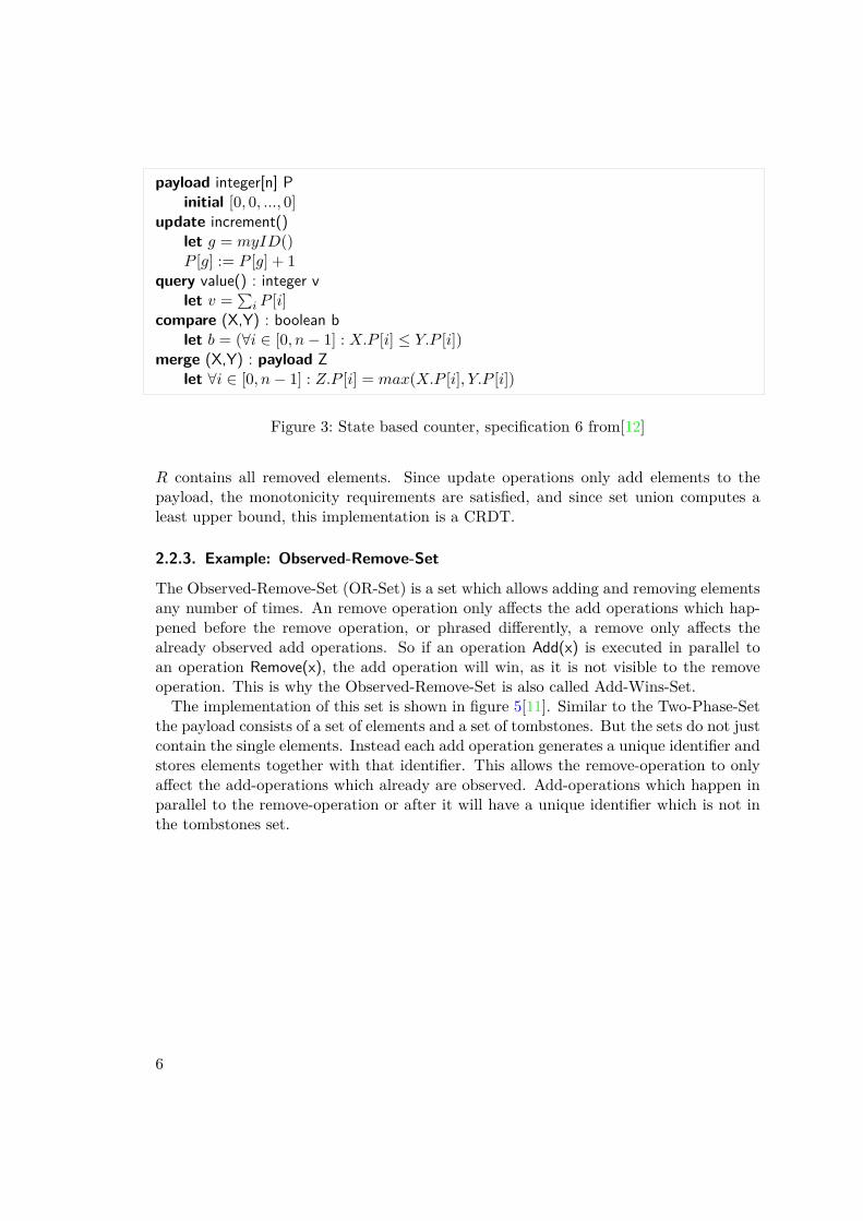
payload integer[n] Pinitial [0, 0, ..., 0]
update increment()let g = myID()P [g] := P [g] + 1
query value() : integer vlet v =
∑i P [i]
compare (X,Y) : boolean blet b = (∀i ∈ [0, n− 1] : X.P [i] ≤ Y.P [i])
merge (X,Y) : payload Zlet ∀i ∈ [0, n− 1] : Z.P [i] = max(X.P [i], Y.P [i])
Figure 3: State based counter, specification 6 from[12]
R contains all removed elements. Since update operations only add elements to thepayload, the monotonicity requirements are satisfied, and since set union computes aleast upper bound, this implementation is a CRDT.
2.2.3. Example: Observed-Remove-Set
The Observed-Remove-Set (OR-Set) is a set which allows adding and removing elementsany number of times. An remove operation only affects the add operations which hap-pened before the remove operation, or phrased differently, a remove only affects thealready observed add operations. So if an operation Add(x) is executed in parallel toan operation Remove(x), the add operation will win, as it is not visible to the removeoperation. This is why the Observed-Remove-Set is also called Add-Wins-Set.The implementation of this set is shown in figure 5[11]. Similar to the Two-Phase-Set
the payload consists of a set of elements and a set of tombstones. But the sets do not justcontain the single elements. Instead each add operation generates a unique identifier andstores elements together with that identifier. This allows the remove-operation to onlyaffect the add-operations which already are observed. Add-operations which happen inparallel to the remove-operation or after it will have a unique identifier which is not inthe tombstones set.
6
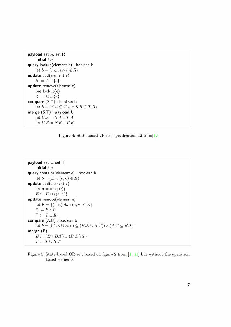
payload set A, set Rinitial ∅, ∅
query lookup(element e) : boolean blet b = (e ∈ A ∧ e /∈ R)
update add(element e)A := A ∪ {e}
update remove(element e)pre lookup(e)R := R ∪ {e}
compare (S,T) : boolean blet b = (S.A ⊆ T.A ∧ S.R ⊆ T.R)
merge (S,T) : payload Ulet U.A = S.A ∪ T.Alet U.R = S.R ∪ T.R
Figure 4: State-based 2P-set, specification 12 from[12]
payload set E, set Tinitial ∅, ∅
query contains(element e) : boolean blet b = (∃n : (e, n) ∈ E)
update add(element e)let n = unique()E := E ∪ {(e, n)}
update remove(element e)let R = {(e, n)|∃n : (e, n) ∈ E}E := E \RT := T ∪R
compare (A,B) : boolean blet b = ((A.E ∪A.T ) ⊆ (B.E ∪B.T )) ∧ (A.T ⊆ B.T )
merge (B)E := (E \B.T ) ∪ (B.E \ T )T := T ∪B.T
Figure 5: State-based OR-set, based on figure 2 from [1, 11] but without the operationbased elements
7

3. System Model for State Based Data TypesTo be able to formally reason about data types, a formal model of the system is needed.The formal model has to be suitable for the Isabelle proof assistant tool. It has to reflectthe reality in a way, that the results proven with the model can be transferred to the realworld. At the same time, the model must be simple and abstract from lower level details,so that the proofs can focus on the essential aspects without getting too technical.When designing a formal model, there always is a trade-off between simplicity and
generality. In this chapter a system model for reasoning about state based CRDTs ispresented along with the design decisions taken.
3.1. Overview
The model considers only one instance of a CRDT. For the purpose of this master’s thesisthis is sufficient as it is not a goal to study the interplay between several objects, whichwould have been important when considering transactions or programs interacting withseveral objects in an interweaved way. Instead this thesis focuses on the behavior of oneobject which interacts with its environment. The environment is not modeled explicitly,but instead the system model uses traces which capture the interactions between theenvironment and the different replicas of the data type instance. The trace also cap-tures the interactions between the replicas, which are the merge operations. The mergeoperations happen independently from the update operations. The traces and executionsemantics are explained in more detail later.The number of replicas is arbitrary but fixed in the system model, which means adding
and removing replicas at runtime is not part of the model. In practice this is a necessaryfeature, and it requires some additional work to implement this correctly. However, thebasic mechanics of the CRDTs are not influenced by this and dynamically adding andremoving replicas can in parts be represented by a model with a fixed number of replicas.Removing a replica can be represented by no longer sending any messages to a replica.Adding a replica can be represented by having a replica, which does not receive anymessages until it is “added” to the system.Updates are executed atomically. Immediately after every update, the new state of
the replica is implicitly sent to all other replicas. The other replicas can receive this stateat any time in the future and merge it with their own state. It is also possible that theynever receive the state or receive the same state multiple times. The model does notrestrict the order in which such merge messages are delivered. The only assumptionson message delivery are, that message contents are not corrupted, and the obviousassumption that messages cannot be received before they are sent. The assumption thatmessages are not corrupted is necessary in order prove any property about the behaviorof the system. If messages could be corrupted in arbitrary ways, the system would beunpredictable.An alternative approach to the implicit sending of messages, would be to have an
explicit send-action. This is what has been done in Replicated Data Types: Specification,Verification, Optimality[3], where send operations are explicit and are also allowed to
9
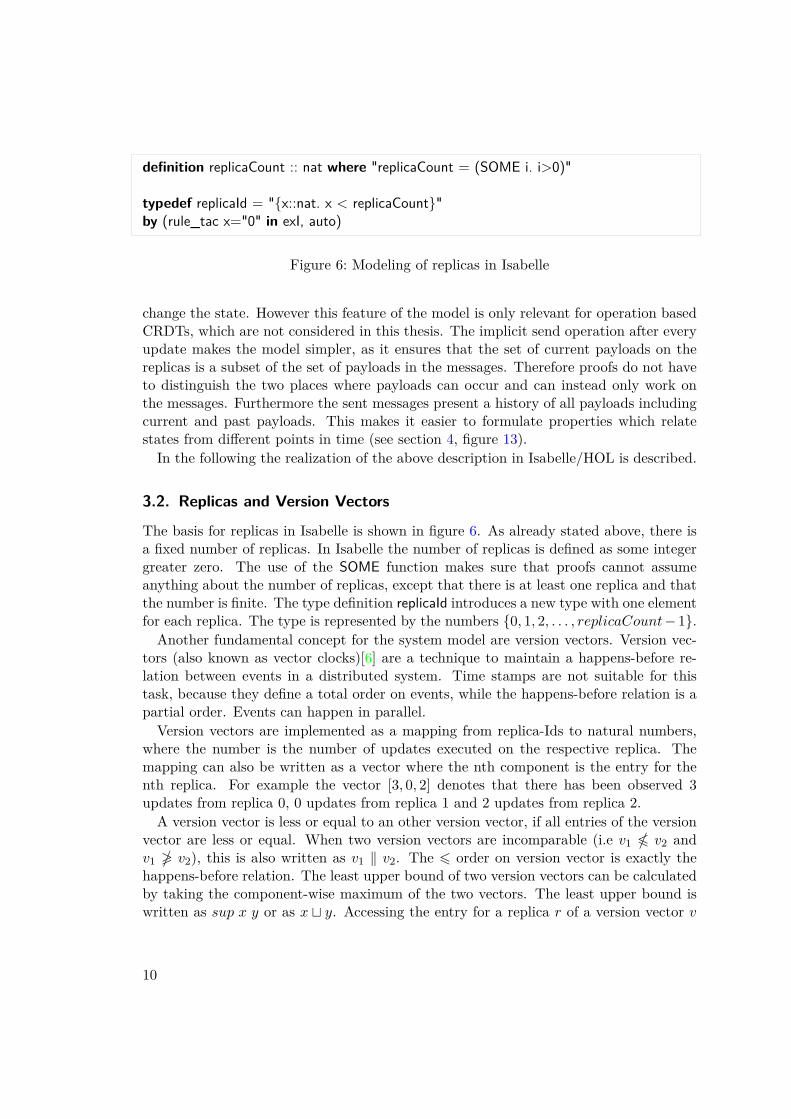
definition replicaCount :: nat where "replicaCount = (SOME i. i>0)"
typedef replicaId = "{x::nat. x < replicaCount}"by (rule_tac x="0" in exI, auto)
Figure 6: Modeling of replicas in Isabelle
change the state. However this feature of the model is only relevant for operation basedCRDTs, which are not considered in this thesis. The implicit send operation after everyupdate makes the model simpler, as it ensures that the set of current payloads on thereplicas is a subset of the set of payloads in the messages. Therefore proofs do not haveto distinguish the two places where payloads can occur and can instead only work onthe messages. Furthermore the sent messages present a history of all payloads includingcurrent and past payloads. This makes it easier to formulate properties which relatestates from different points in time (see section 4, figure 13).In the following the realization of the above description in Isabelle/HOL is described.
3.2. Replicas and Version Vectors
The basis for replicas in Isabelle is shown in figure 6. As already stated above, there isa fixed number of replicas. In Isabelle the number of replicas is defined as some integergreater zero. The use of the SOME function makes sure that proofs cannot assumeanything about the number of replicas, except that there is at least one replica and thatthe number is finite. The type definition replicaId introduces a new type with one elementfor each replica. The type is represented by the numbers {0, 1, 2, . . . , replicaCount− 1}.Another fundamental concept for the system model are version vectors. Version vec-
tors (also known as vector clocks)[6] are a technique to maintain a happens-before re-lation between events in a distributed system. Time stamps are not suitable for thistask, because they define a total order on events, while the happens-before relation is apartial order. Events can happen in parallel.Version vectors are implemented as a mapping from replica-Ids to natural numbers,
where the number is the number of updates executed on the respective replica. Themapping can also be written as a vector where the nth component is the entry for thenth replica. For example the vector [3, 0, 2] denotes that there has been observed 3updates from replica 0, 0 updates from replica 1 and 2 updates from replica 2.A version vector is less or equal to an other version vector, if all entries of the version
vector are less or equal. When two version vectors are incomparable (i.e v1 v2 andv1 � v2), this is also written as v1 ‖ v2. The 6 order on version vector is exactly thehappens-before relation. The least upper bound of two version vectors can be calculatedby taking the component-wise maximum of the two vectors. The least upper bound iswritten as sup x y or as x t y. Accessing the entry for a replica r of a version vector v
10
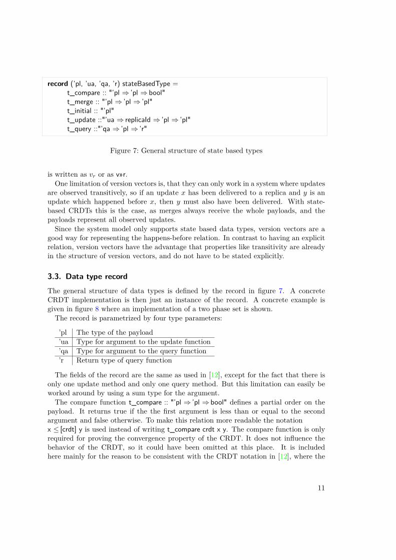
record (’pl, ’ua, ’qa, ’r) stateBasedType =t_compare :: "’pl ⇒ ’pl ⇒ bool"t_merge :: "’pl ⇒ ’pl ⇒ ’pl"t_initial :: "’pl"t_update ::"’ua ⇒ replicaId ⇒ ’pl ⇒ ’pl"t_query ::"’qa ⇒ ’pl ⇒ ’r"
Figure 7: General structure of state based types
is written as vr or as v»r.One limitation of version vectors is, that they can only work in a system where updates
are observed transitively, so if an update x has been delivered to a replica and y is anupdate which happened before x, then y must also have been delivered. With state-based CRDTs this is the case, as merges always receive the whole payloads, and thepayloads represent all observed updates.Since the system model only supports state based data types, version vectors are a
good way for representing the happens-before relation. In contrast to having an explicitrelation, version vectors have the advantage that properties like transitivity are alreadyin the structure of version vectors, and do not have to be stated explicitly.
3.3. Data type record
The general structure of data types is defined by the record in figure 7. A concreteCRDT implementation is then just an instance of the record. A concrete example isgiven in figure 8 where an implementation of a two phase set is shown.The record is parametrized by four type parameters:
’pl The type of the payload’ua Type for argument to the update function’qa Type for argument to the query function’r Return type of query function
The fields of the record are the same as used in [12], except for the fact that there isonly one update method and only one query method. But this limitation can easily beworked around by using a sum type for the argument.The compare function t_compare :: "’pl ⇒ ’pl ⇒ bool" defines a partial order on the
payload. It returns true if the the first argument is less than or equal to the secondargument and false otherwise. To make this relation more readable the notationx ≤ [crdt] y is used instead of writing t_compare crdt x y. The compare function is onlyrequired for proving the convergence property of the CRDT. It does not influence thebehavior of the CRDT, so it could have been omitted at this place. It is includedhere mainly for the reason to be consistent with the CRDT notation in [12], where the
11
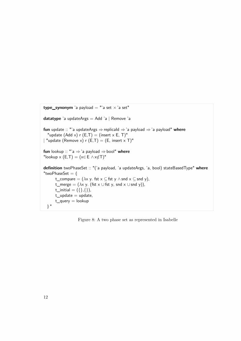
type_synonym ’a payload = "’a set × ’a set"
datatype ’a updateArgs = Add ’a | Remove ’a
fun update :: "’a updateArgs ⇒ replicaId ⇒ ’a payload ⇒ ’a payload" where"update (Add x) r (E,T) = (insert x E, T)"
| "update (Remove x) r (E,T) = (E, insert x T)"
fun lookup :: "’a ⇒ ’a payload ⇒ bool" where"lookup x (E,T) = (x∈E ∧ x/∈T)"
definition twoPhaseSet :: "(’a payload, ’a updateArgs, ’a, bool) stateBasedType" where"twoPhaseSet = L
t_compare = (λx y. fst x ⊆ fst y ∧ snd x ⊆ snd y),t_merge = (λx y. (fst x ∪ fst y, snd x ∪ snd y)),t_initial = ({},{}),t_update = update,t_query = lookup
M "
Figure 8: A two phase set as represented in Isabelle
12
compare function is also noted as part of the data type.The merge function t_merge :: "’pl ⇒ ’pl ⇒ ’pl" defines how two payloads are merged
together. An alternative notation for t_merge crdt x y is x t [crdt] y.The initial payload is determined by the field t_initial :: "’pl". Note that the initial
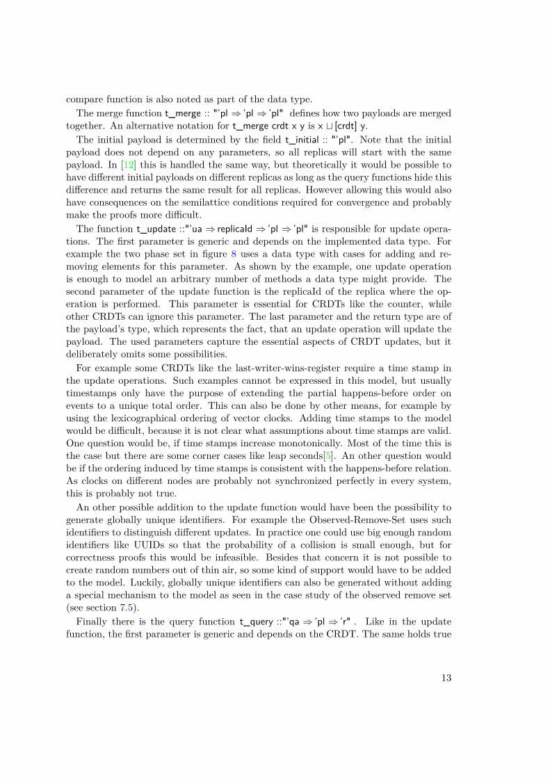
payload does not depend on any parameters, so all replicas will start with the samepayload. In [12] this is handled the same way, but theoretically it would be possible tohave different initial payloads on different replicas as long as the query functions hide thisdifference and returns the same result for all replicas. However allowing this would alsohave consequences on the semilattice conditions required for convergence and probablymake the proofs more difficult.The function t_update ::"’ua ⇒ replicaId ⇒ ’pl ⇒ ’pl" is responsible for update opera-
tions. The first parameter is generic and depends on the implemented data type. Forexample the two phase set in figure 8 uses a data type with cases for adding and re-moving elements for this parameter. As shown by the example, one update operationis enough to model an arbitrary number of methods a data type might provide. Thesecond parameter of the update function is the replicaId of the replica where the op-eration is performed. This parameter is essential for CRDTs like the counter, whileother CRDTs can ignore this parameter. The last parameter and the return type are ofthe payload’s type, which represents the fact, that an update operation will update thepayload. The used parameters capture the essential aspects of CRDT updates, but itdeliberately omits some possibilities.For example some CRDTs like the last-writer-wins-register require a time stamp in
the update operations. Such examples cannot be expressed in this model, but usuallytimestamps only have the purpose of extending the partial happens-before order onevents to a unique total order. This can also be done by other means, for example byusing the lexicographical ordering of vector clocks. Adding time stamps to the modelwould be difficult, because it is not clear what assumptions about time stamps are valid.One question would be, if time stamps increase monotonically. Most of the time this isthe case but there are some corner cases like leap seconds[5]. An other question wouldbe if the ordering induced by time stamps is consistent with the happens-before relation.As clocks on different nodes are probably not synchronized perfectly in every system,this is probably not true.An other possible addition to the update function would have been the possibility to
generate globally unique identifiers. For example the Observed-Remove-Set uses suchidentifiers to distinguish different updates. In practice one could use big enough randomidentifiers like UUIDs so that the probability of a collision is small enough, but forcorrectness proofs this would be infeasible. Besides that concern it is not possible tocreate random numbers out of thin air, so some kind of support would have to be addedto the model. Luckily, globally unique identifiers can also be generated without addinga special mechanism to the model as seen in the case study of the observed remove set(see section 7.5).Finally there is the query function t_query ::"’qa ⇒ ’pl ⇒ ’r" . Like in the update
function, the first parameter is generic and depends on the CRDT. The same holds true
13
for the return type. Besides the first parameter the result of a query only depends onthe local payload of the queried replica.Queries and updates could theoretically be combined into one function of type ’ua⇒ replicaId ⇒ ’pl ⇒ (’pl × ’r). This would make the model more powerful, as it wouldallow operations which atomically modify the state and return a value. For example theAdd operation on sets could return whether the element already was in the set. Insteadthe model requires to first evaluate a query and then execute an update. This is not abig restriction for the model, as queries can be evaluated on a specific state. So there isno problem of race conditions, as there would be when doing the same in a real system.An advantage of a separate query function is, that some statements are easier to express.For example specifications often use queries for describing pre- and post-conditions andside effects on the payload would be distractive there.
3.4. Traces and Actions
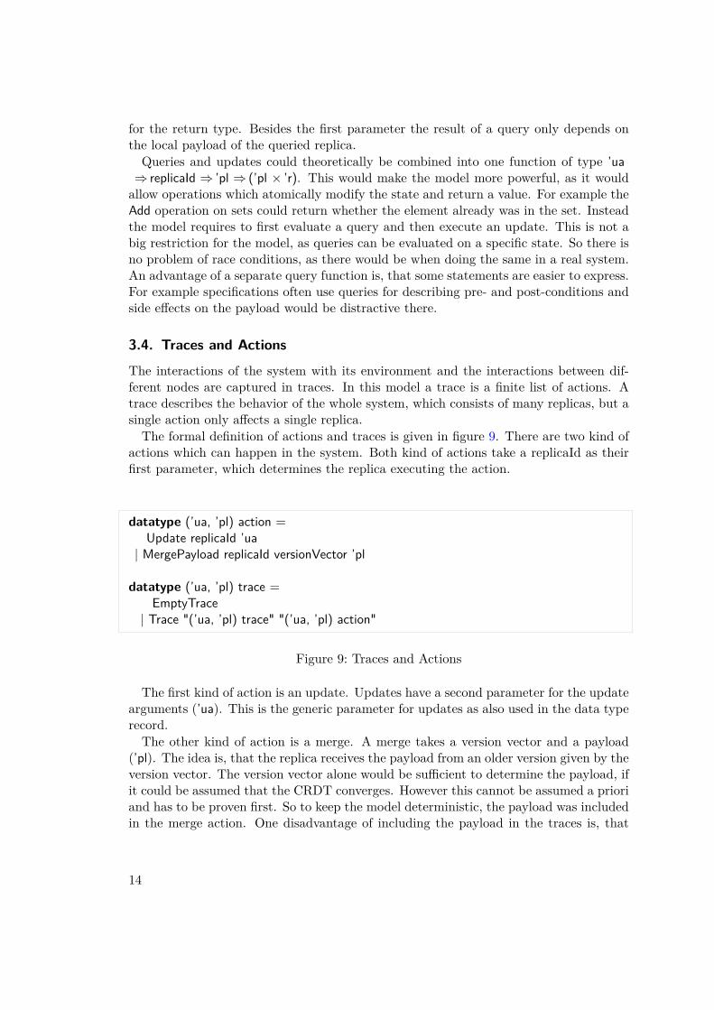
The interactions of the system with its environment and the interactions between dif-ferent nodes are captured in traces. In this model a trace is a finite list of actions. Atrace describes the behavior of the whole system, which consists of many replicas, but asingle action only affects a single replica.The formal definition of actions and traces is given in figure 9. There are two kind of
actions which can happen in the system. Both kind of actions take a replicaId as theirfirst parameter, which determines the replica executing the action.
datatype (’ua, ’pl) action =Update replicaId ’ua
| MergePayload replicaId versionVector ’pl
datatype (’ua, ’pl) trace =EmptyTrace
| Trace "(’ua, ’pl) trace" "(’ua, ’pl) action"
Figure 9: Traces and Actions
The first kind of action is an update. Updates have a second parameter for the updatearguments (’ua). This is the generic parameter for updates as also used in the data typerecord.The other kind of action is a merge. A merge takes a version vector and a payload
(’pl). The idea is, that the replica receives the payload from an older version given by theversion vector. The version vector alone would be sufficient to determine the payload, ifit could be assumed that the CRDT converges. However this cannot be assumed a prioriand has to be proven first. So to keep the model deterministic, the payload was includedin the merge action. One disadvantage of including the payload in the traces is, that
14
it exposes implementation details in the traces, which makes it a bit more difficult tocompare different implementations of the same abstract CRDT. An alternative approachwould have been to use unique identifiers instead of the version vectors, so that therecould be a unique mapping from identifiers to payloads.As an example, consider the execution shown in figure 10. This execution can be
described by the following trace, assuming the underlying implementation is a Two-Phase-Set as introduced in section 2.2.2, where the payload consists of an elements- anda tombstones-set:[Update(r1, add(x)),Update(r2, add(y)),MergePayload(r3, [0, 1, 0], ({y}, {})),MergePayload(r2, [1, 0, 0], ({x}, {})),Update(r3, add(x)),Update(r2, remove(x)),Update(r3, remove(y)),MergePayload(r2, [0, 1, 2], ({x, y}, {y}))].
Figure 10: Example Execution
Basing the semantics of the model on traces allows the semantics to be deterministic.For one given trace there is only one possible execution. This makes it easier to reasonabout the system. But from the perspective of a client, who cannot see the internalmerge operations happening in the system, the semantics are still nondeterministic.Furthermore traces have the advantage, that it is easy to do a proof by induction
over traces, whereas an induction over a graph, for example the happens-before graph,is more difficult.
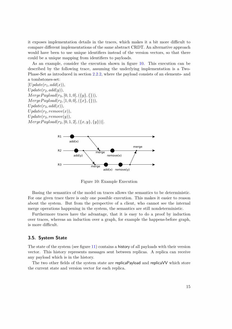
3.5. System State
The state of the system (see figure 11) contains a history of all payloads with their versionvector. This history represents messages sent between replicas. A replica can receiveany payload which is in the history.The two other fields of the system state are replicaPayload and replicaVV which store
the current state and version vector for each replica.
15
type_synonym ’pl history = "(versionVector × ’pl) set"
record ’pl systemState =replicaPayload :: "replicaId ⇒ ’pl"replicaVV :: "replicaId ⇒ versionVector"history :: "’pl history"
Figure 11: System State
Note that (replicaV V r, replicaPayload r) ∈ history holds for every replica. Com-pared to having an explicit message channel and explicit sending this makes the analysisless technical in some cases. Nevertheless it is still clear that the results could easily betransferred to a model with explicit message sending.
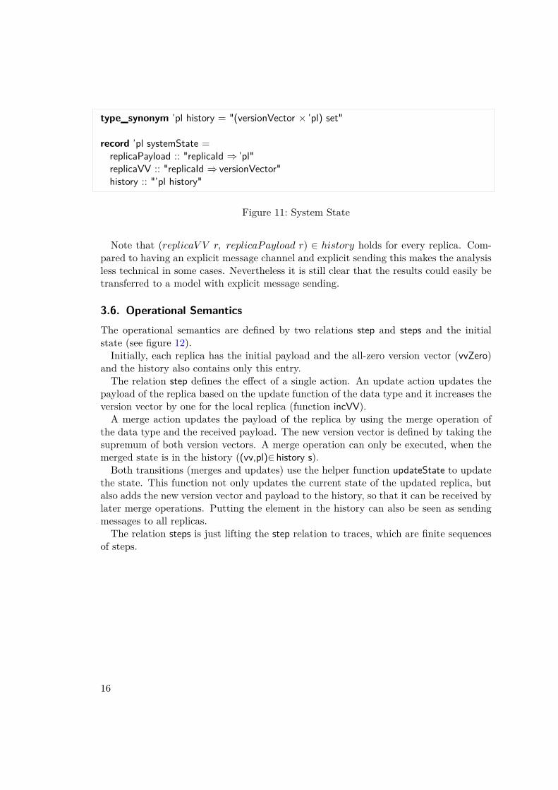
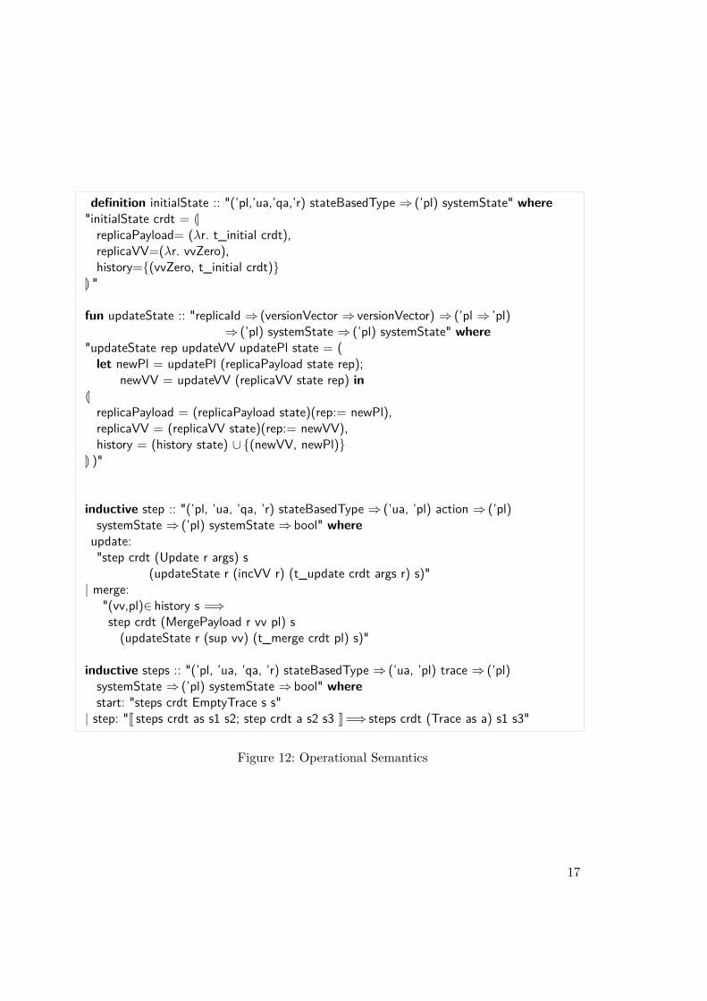
3.6. Operational SemanticsThe operational semantics are defined by two relations step and steps and the initialstate (see figure 12).Initially, each replica has the initial payload and the all-zero version vector (vvZero)
and the history also contains only this entry.The relation step defines the effect of a single action. An update action updates the
payload of the replica based on the update function of the data type and it increases theversion vector by one for the local replica (function incVV).A merge action updates the payload of the replica by using the merge operation of
the data type and the received payload. The new version vector is defined by taking thesupremum of both version vectors. A merge operation can only be executed, when themerged state is in the history ((vv,pl)∈ history s).Both transitions (merges and updates) use the helper function updateState to update
the state. This function not only updates the current state of the updated replica, butalso adds the new version vector and payload to the history, so that it can be received bylater merge operations. Putting the element in the history can also be seen as sendingmessages to all replicas.The relation steps is just lifting the step relation to traces, which are finite sequences
of steps.
16
definition initialState :: "(’pl,’ua,’qa,’r) stateBasedType ⇒ (’pl) systemState" where"initialState crdt = LreplicaPayload= (λr. t_initial crdt),replicaVV=(λr. vvZero),history={(vvZero, t_initial crdt)}
M "
fun updateState :: "replicaId ⇒ (versionVector ⇒ versionVector) ⇒ (’pl ⇒ ’pl)⇒ (’pl) systemState ⇒ (’pl) systemState" where
"updateState rep updateVV updatePl state = (let newPl = updatePl (replicaPayload state rep);
newVV = updateVV (replicaVV state rep) inLreplicaPayload = (replicaPayload state)(rep:= newPl),replicaVV = (replicaVV state)(rep:= newVV),history = (history state) ∪ {(newVV, newPl)}
M )"
inductive step :: "(’pl, ’ua, ’qa, ’r) stateBasedType ⇒ (’ua, ’pl) action ⇒ (’pl)systemState ⇒ (’pl) systemState ⇒ bool" whereupdate:"step crdt (Update r args) s
(updateState r (incVV r) (t_update crdt args r) s)"| merge:
"(vv,pl)∈ history s =⇒step crdt (MergePayload r vv pl) s(updateState r (sup vv) (t_merge crdt pl) s)"
inductive steps :: "(’pl, ’ua, ’qa, ’r) stateBasedType ⇒ (’ua, ’pl) trace ⇒ (’pl)systemState ⇒ (’pl) systemState ⇒ bool" wherestart: "steps crdt EmptyTrace s s"
| step: "J steps crdt as s1 s2; step crdt a s2 s3 K =⇒ steps crdt (Trace as a) s1 s3"
Figure 12: Operational Semantics
17

4. ConsistencyOne of the most important properties of CRDTs is the provided consistency guarantee.As updates can be executed on a single replica, CRDTs cannot provide strong consis-tency guarantees, where it would be guaranteed that the system behaves like it wasa centralized system with a single replica. Instead CRDTs only guarantee a form ofeventual consistency.
4.1. Eventual Consistency
There are different definitions of eventual consistency, but intuitively they all capturethe idea, that not all replicas will necessarily provide the same answer to a query andonly after some time the replicas will converge and eventually return the same answerto queries.In [12] the definition of eventual convergence consists of a safety property and a liveness
property. The liveness property states that every update operation is eventually deliveredto all replicas. The safety property states, that if two replicas have seen the same set ofupdates, then their abstract state has to be the same, where the abstract state is definedas the state which can be observed by queries.In [2] roughly the same liveness property is defined more formally as follows:
∀a ∈ A. ¬(∃ infinitely many b ∈ A. sameobj(a, b) ∧ ¬(a vis−−→ b))
Here A is the set of actions and vis−−→ denotes the visibility relation between actions. Sothe definition states that for every action, there cannot be an infinite number of actions,which have not seen the former action.The problem with these kind of liveness definition is that it can only be applied to
infinite executions and the system model introduced in section 3 only models finiteexecutions. With such a model it is only possible to define the liveness property as thepossibility to reach a desired state: In every reachable state of the system it should bepossible to execute a number of steps, so that any update operation is visible on anyreplica. However this property trivially holds, as merge operations with previous statesare always enabled in the model, so it is always possible to perform a merge operationin order to get visibility.As the system model cannot make any nontrivial liveness guarantees, the safety prop-
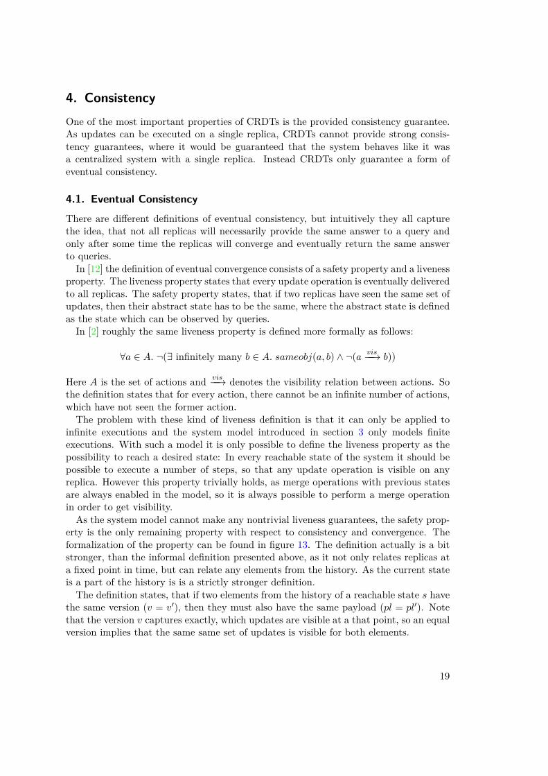
erty is the only remaining property with respect to consistency and convergence. Theformalization of the property can be found in figure 13. The definition actually is a bitstronger, than the informal definition presented above, as it not only relates replicas ata fixed point in time, but can relate any elements from the history. As the current stateis a part of the history is is a strictly stronger definition.The definition states, that if two elements from the history of a reachable state s have
the same version (v = v′), then they must also have the same payload (pl = pl′). Notethat the version v captures exactly, which updates are visible at a that point, so an equalversion implies that the same same set of updates is visible for both elements.
19
definition convergent_crdt :: "(’pl,’ua’,’qa,’r) stateBasedType ⇒ bool" where"convergent_crdt crdt = (∀tr s v pl v’ pl’.steps crdt tr (initialState crdt) s∧ (v , pl ) ∈ history s∧ (v’, pl’) ∈ history s∧ v=v’ −→ pl=pl’)"
Figure 13: Convergence definition 1
definition convergent_crdt2 :: "(’pl,’ua’,’qa,’r) stateBasedType ⇒ bool" where"convergent_crdt2 crdt = (∀tr s v pl v’ pl’.steps crdt tr (initialState crdt) s∧ (v , pl ) ∈ history s∧ (v’, pl’) ∈ history s∧ v≤ v’ −→ pl ≤ [crdt] pl’)"
Figure 14: Convergence definition 2
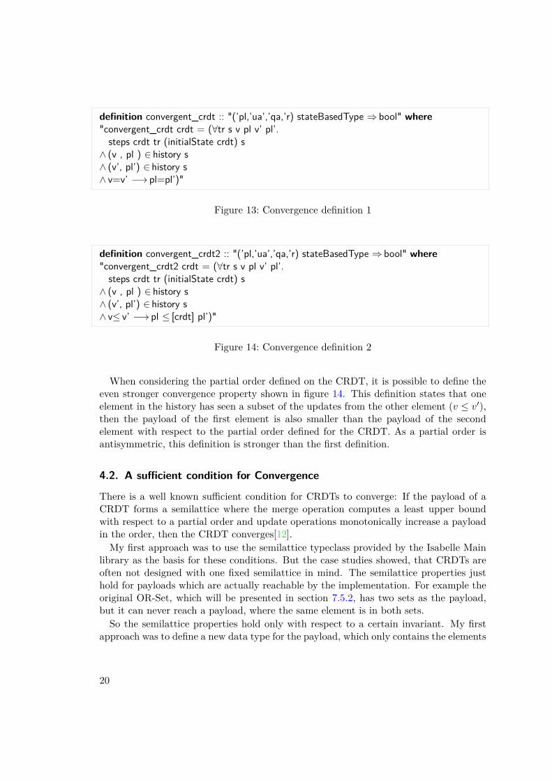
When considering the partial order defined on the CRDT, it is possible to define theeven stronger convergence property shown in figure 14. This definition states that oneelement in the history has seen a subset of the updates from the other element (v ≤ v′),then the payload of the first element is also smaller than the payload of the secondelement with respect to the partial order defined for the CRDT. As a partial order isantisymmetric, this definition is stronger than the first definition.
4.2. A sufficient condition for Convergence
There is a well known sufficient condition for CRDTs to converge: If the payload of aCRDT forms a semilattice where the merge operation computes a least upper boundwith respect to a partial order and update operations monotonically increase a payloadin the order, then the CRDT converges[12].My first approach was to use the semilattice typeclass provided by the Isabelle Main
library as the basis for these conditions. But the case studies showed, that CRDTs areoften not designed with one fixed semilattice in mind. The semilattice properties justhold for payloads which are actually reachable by the implementation. For example theoriginal OR-Set, which will be presented in section 7.5.2, has two sets as the payload,but it can never reach a payload, where the same element is in both sets.So the semilattice properties hold only with respect to a certain invariant. My first
approach was to define a new data type for the payload, which only contains the elements
20
satisfying the invariant. However this approach led to a lot of proof steps, which werejust about conversions between the newly defined data types and standard data types.Therefore I decided to use standard data types instead and define a separate invariant,although this had the drawback, that it was no longer possible to use the semilatticetypeclass. So a lot of semilattice related lemmas from the Main library had to be portedto the new approach.The invariant used has the following type:
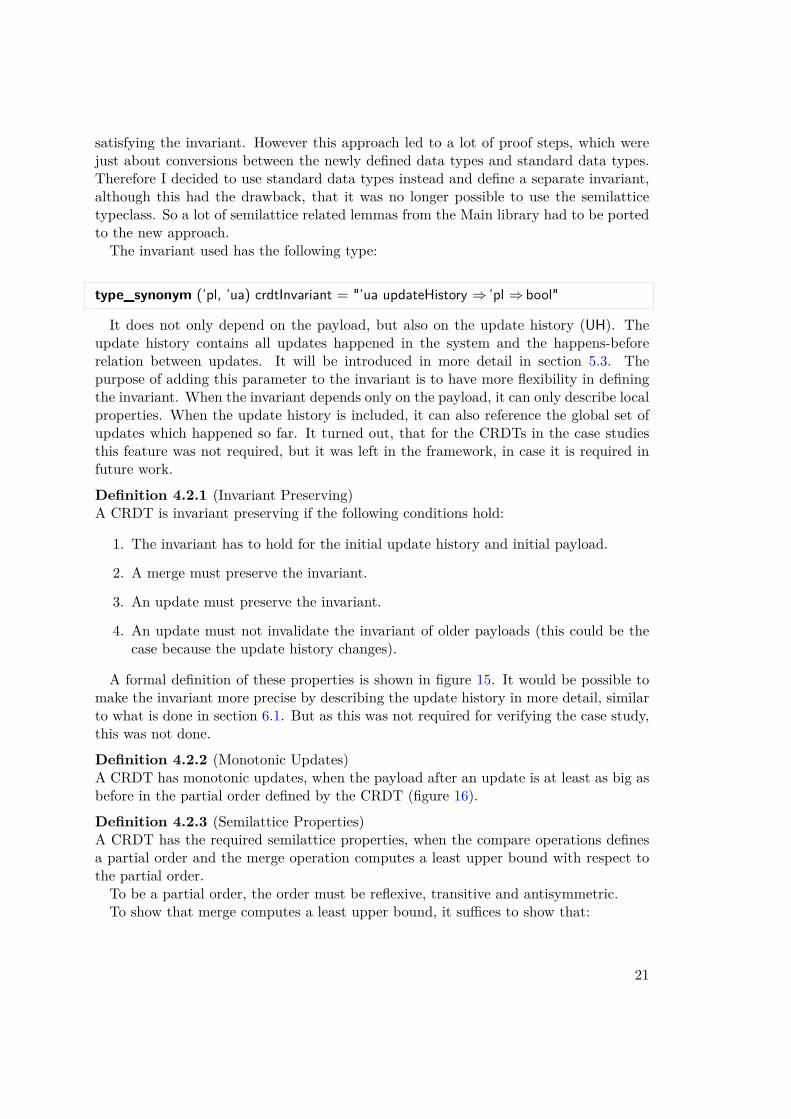
type_synonym (’pl, ’ua) crdtInvariant = "’ua updateHistory ⇒ ’pl ⇒ bool"
It does not only depend on the payload, but also on the update history (UH). Theupdate history contains all updates happened in the system and the happens-beforerelation between updates. It will be introduced in more detail in section 5.3. Thepurpose of adding this parameter to the invariant is to have more flexibility in definingthe invariant. When the invariant depends only on the payload, it can only describe localproperties. When the update history is included, it can also reference the global set ofupdates which happened so far. It turned out, that for the CRDTs in the case studiesthis feature was not required, but it was left in the framework, in case it is required infuture work.
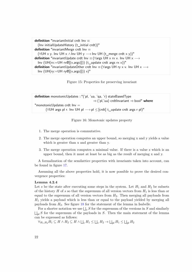
Definition 4.2.1 (Invariant Preserving)A CRDT is invariant preserving if the following conditions hold:
1. The invariant has to hold for the initial update history and initial payload.
2. A merge must preserve the invariant.
3. An update must preserve the invariant.
4. An update must not invalidate the invariant of older payloads (this could be thecase because the update history changes).
A formal definition of these properties is shown in figure 15. It would be possible tomake the invariant more precise by describing the update history in more detail, similarto what is done in section 6.1. But as this was not required for verifying the case study,this was not done.
Definition 4.2.2 (Monotonic Updates)A CRDT has monotonic updates, when the payload after an update is at least as big asbefore in the partial order defined by the CRDT (figure 16).
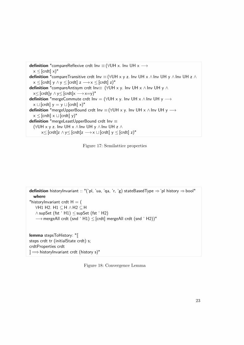
Definition 4.2.3 (Semilattice Properties)A CRDT has the required semilattice properties, when the compare operations definesa partial order and the merge operation computes a least upper bound with respect tothe partial order.To be a partial order, the order must be reflexive, transitive and antisymmetric.To show that merge computes a least upper bound, it suffices to show that:
21
definition "invariantInitial crdt Inv ≡(Inv initialUpdateHistory (t_initial crdt))"
definition "invariantMerge crdt Inv ≡(∀UH x y. Inv UH x ∧ Inv UH y −→ Inv UH (t_merge crdt x y))"
definition "invariantUpdate crdt Inv ≡ (∀args UH x rx v. Inv UH x −→Inv (UH(rx:=UH rx@[(v,args)])) (t_update crdt args rx x))"
definition "invariantUpdateOther crdt Inv ≡ (∀args UH ry x v. Inv UH x −→Inv (UH(ry:=UH ry@[(v,args)])) x)"
Figure 15: Properties for preserving invariant
definition monotonicUpdates ::"(’pl, ’ua, ’qa, ’r) stateBasedType⇒ (’pl,’ua) crdtInvariant ⇒ bool" where
"monotonicUpdates crdt Inv =(∀UH args pl r. Inv UH pl −→ pl ≤ [crdt] t_update crdt args r pl)"
Figure 16: Monotonic updates property
1. The merge operation is commutative.
2. The merge operation computes an upper bound, so merging x and y yields a valuewhich is greater than x and greater than y.
3. The merge operation computes a minimal value. If there is a value z which is anupper bound, then it must at least be as big as the result of merging x and y.
A formalization of the semilattice properties with invariants taken into account, canbe found in figure 17.
Assuming all the above properties hold, it is now possible to prove the desired con-vergence properties:
Lemma 4.2.4Let s be the state after executing some steps in the system. Let H1 and H2 be subsetsof the history H of s so that the supremum of all version vectors from H1 is less than orequal to the supremum of all version vectors from H2. Then merging all payloads fromH1 yields a payload which is less than or equal to the payload yielded by merging allpayloads from H2. See figure 18 for the statement of the lemma in Isabelle.For a shorter notation we use
⊔v S for the supremum of the versions in S and similarly⊔
pl S for the supremum of the payloads in S. Then the main statement of the lemmacan be expressed as follows:∀H1,H2H1 ⊆ H ∧H2 ⊆ H ∧
⊔v H1 ≤
⊔v H2 →
⊔pl H1 ≤
⊔pl H2
22
definition "compareReflexive crdt Inv ≡ (∀UH x. Inv UH x −→x ≤ [crdt] x)"
definition "compareTransitive crdt Inv ≡ (∀UH x y z. Inv UH x ∧ Inv UH y ∧ Inv UH z ∧x ≤ [crdt] y ∧ y ≤ [crdt] z −→ x ≤ [crdt] z)"
definition "compareAntisym crdt Inv≡ (∀UH x y. Inv UH x ∧ Inv UH y ∧x≤ [crdt]y ∧ y≤ [crdt]x −→ x=y)"
definition "mergeCommute crdt Inv = (∀UH x y. Inv UH x ∧ Inv UH y −→x t [crdt] y = y t [crdt] x)"
definition "mergeUpperBound crdt Inv ≡ (∀UH x y. Inv UH x ∧ Inv UH y −→x ≤ [crdt] x t [crdt] y)"
definition "mergeLeastUpperBound crdt Inv ≡(∀UH x y z. Inv UH x ∧ Inv UH y ∧ Inv UH z ∧
x≤ [crdt]z ∧ y≤ [crdt]z −→ x t [crdt] y ≤ [crdt] z)"
Figure 17: Semilattice properties
definition historyInvariant :: "(’pl, ’ua, ’qa, ’r, ’g) stateBasedType ⇒ ’pl history ⇒ bool"where
"historyInvariant crdt H = (∀H1 H2. H1 ⊆H ∧H2 ⊆H∧ supSet (fst ‘ H1) ≤ supSet (fst ‘ H2)−→mergeAll crdt (snd ‘ H1) ≤ [crdt] mergeAll crdt (snd ‘ H2))"
lemma stepsToHistory: "Jsteps crdt tr (initialState crdt) s;crdtProperties crdtK =⇒ historyInvariant crdt (history s)"
Figure 18: Convergence Lemma
23
Proof. By induction over the steps.
Initial state In the initial state the history contains only one element:([0, . . . , 0], tinitial(crdt)). So the claim follows by the reflexivity of the partial order.
Update After an update operation, one new element is in the history.Let enew be the new element in the history and eold the element before the update.Let H1 and H2 be two subsets of the new history with
⊔v H1 ≤
⊔v H2. There are four
cases to be considered:
Case 1: The new element is neither in H1 nor H2. In this case the claim follows directlyfrom the induction hypothesis.
Case 2: The new element is only in H1.Then we must have
⊔v H1 >
⊔v H2, because the versions in H1 include enew. The
version vector of the new element is higher than all other version vectors in the history.This is a contradiction to the assumption that
⊔v H1 ≤
⊔v H2.
Case 3: The new element is only in H2.Consider the two sets H ′
1 = H1 and H ′2 = H2\{enew} ∪ {eold}.
Then⊔
v H′1 ≤
⊔v H
′2, because the version vector is only decreased in the local com-
ponent, where the old version vector was already maximal.So by the induction hypothesis, we get that
⊔pl H
′1 ≤
⊔pl H
′2. Because updates are
monotonically increasing we also have⊔
pl H′2 ≤
⊔pl H2. The claim follows by transitivity.
Case 4: The new element is in H1 and H2.Similar to case 3, consider the two sets
H ′1 = H1\{enew} ∪ {eold}
H ′2 = H2\{enew} ∪ {eold}
Again, we have⊔
v H′1 ≤
⊔v H
′2 and thus
⊔pl H
′1 ≤
⊔pl H
′2.
Because the merge operation is associative, the element eold can be extracted from theset: ⊔
pl
H ′1 = eold t
⊔pl
(H1\{enew}) ≤ eold t⊔pl
(H2\{enew}) =⊔pl
H ′2
By the monotonicity of merges we can replace eold by the bigger enew and preservethe order:
enew t⊔pl
(H1\{enew}) ≤ enew t⊔pl
(H2\{enew})
24
By using associativity of merges we can move the element enew inside the overallsupremum: ⊔
pl
H1 ≤⊔pl
H2
This finishes the case for updates.
Merge After a merge operation there is one new element enew in the history, which isthe supremum or merge of two elements ea and eb from the old history.If enew is in H1, we can take H ′
1 = H1\{enew} ∪ {ea, eb}. Then⊔
v H′1 =
⊔v H1 and⊔
pl H′1 =
⊔pl H1 by associativity. If enew is not in H1, let H ′
1 = H1.The same can be done for H2.Because we have found equivalent sets to H1 and H2 without the new element, the
claim holds by the induction hypothesis.
Theorem 4.2.5 (Convergence of CRDTs)If a CRDT is invariant preserving, has monotonic updates and satisfies the semilatticeproperties, then it converges (as defined in figure 13).
Proof. Let e1 and e2 be elements from the history with version(e1) ≤ version(e2).Lemma 4.2.4 can be instantiated with H1 = {e1} and H2 = {e2}. This yields
payload(e1) ≤ payload(e2).Thus, if version(e1) = version(e2), we get payload(e1) = payload(e2) by the antisym-
metry of the ordering.
25

5. Specification of CRDTsWhile the specification of sequential data types is relatively straight forward, it is de-batable what the best way to specify parallel, distributed data types is. Operationson sequential data types are usually described by pre- and post-conditions[4]. When asequence of operations is given, the pre- and post-conditions can be chained togetherand pre- and post-conditions for the whole sequence can be obtained. This approachcannot be directly transferred to parallel, distributed data types:
1. In general there is no sequence of operations but instead a directed acyclic graph(DAG) of operations, where some operations can happen in parallel.
2. Pre- and post-conditions could be defined with respect to local states or the globalstate.
3. Distributed data types have mechanisms for synchronization. Specifications canchoose to explicitly specify those mechanisms or to keep it implicit.
The remainder of this chapter presents different approaches to specify CRDTs usingthe examples of the counter and the observed-removed set, which were introduced insection 2.2.
Notations. The following notations and conventions are used to describe the differentspecification techniques: The variable s always refers to a state of the whole system.When s is indexed this refers to the state on a single replica. For example sr1 refers tothe state of replica r1. An squiggled arrow with operations written on top denotes, thatthe system changes from the left state to the right state by executing the operations
on top of the arrow. For example sadd(x)
s′ means that the system goes from states to state s′ by executing a add-operation. A capital S denotes the set of all statesreachable from the initial state and Sl is the set of all reachable local states. Operationsare ordered by a happens-before relation which is denoted by ≺.
5.1. Separated sequential and concurrent specifications
In [11] specifications consist of two parts: a sequential specification and a concurrentspecification. Both parts use a notation with pre- and post-conditions to specify theoutcome of operations. The sequential part of the specification is equivalent to speci-fications of sequential data types. The parallel part then specifies how the data typebehaves when several operations are executed in parallel.A sequential specification is given as a set of Hoare-triples. The Hoare-triple {P}op{Q}
requires that Q should hold after operation op whenever P was true before executingthe operation. This definition can be written as follows:
∀s, s′ ∈ Sl • (P (s) ∧ s ops′)→ Q(s′)
27
The parallel specification is also written in a similar style, but instead of just oneoperation it considers several operations executed in parallel. The general form is{P}op1 ‖ op2 ‖ · · · ‖ opn{Q}. The rough idea is that if P holds in a state s, thenexecuting all operations on s independently and then merging the resulting states shouldyield a state where Q holds.When formalizing the idea of parallel specifications, it has to be refined on which
states the pre- and post-condition should hold. For the pre-condition there are somepossibilities:
1. The pre-condition refers to a local state of one replica, which also is the state onwhich all operations are performed.
2. The pre-condition refers to each local states of every affected replicas.
3. The pre-condition refers to the merged state of all affected replicas.
For the post-condition the only reasonable state is the merged state of all the localstates after executing the parallel operations.In the following definition of the semantics for {P}op1 ‖ op2 ‖ · · · ‖ opn{Q}, the pre-
condition has to hold for a local state s. Then starting from this state s, all operationsop1, op2, . . . , opn are executed in parallel, resulting in states s1, . . . , sn. Then, when allthese states are merged into a state s′, the post-condition Q has to hold for s′:
∀s, s1, . . . , sn, s′ ∈ Sl • (P (s) ∧ (∀i s
opisi) ∧ (s
merge(s1);...;merge(sn)s′))→ Q(s′)
5.1.1. Principle of permutation equivalence
The principle of permutation equivalence restricts the choices which can be taken byconcurrent operations. It is not necessary for a CRDT to adhere to this principle, but itis considered good practice. The principle states that if all possible sequential executionsof a set of operations yields a common post-condition, then that post-condition shouldalso hold when the operations are executed in parallel.[11]For two operations the principle can be expressed as:
{P}op1; op2{Q} ∧ {P}op2; op1{Q} −→ {P}op1 ‖ op2{Q}
5.1.2. Example: Counter
Sequential specification:
{val() = i} add(x) {val() = i+ x}
Concurrent specification:
28
{val() = i} add(x1) ‖ · · · ‖ add(xn) {val() = i+ x1 + · · ·+ xn}
The concurrent specification of the counter is already determined by the principle ofpermutation equivalence. Because all operations commute, the post-condition in the con-current specification cannot be chosen differently. Therefore the sequential specificationalone would be sufficient to specify the Counter.
5.1.3. Example: Observed-Remove Set
Sequential specification:
{true} add(e) {e ∈ S}{e ∈ S} add(f) {e ∈ S}
{e /∈ S ∧ e 6= f} add(f) {e /∈ S}{true} remove(e) {e /∈ S}
{e ∈ S ∧ e 6= f} remove(f) {e ∈ S}{e /∈ S} remove(f) {e /∈ S}
The principle of permutation equivalence already fixes the semantics for parallel op-erations which are independent from each other. For example we have:
{true} add(e) ‖ add(f) {e ∈ S ∧ f ∈ S}{e 6= f} add(e) ‖ remove(f) {e ∈ S ∧ f /∈ S}
. . .
The only interesting case is when two operations are conflicting, which only is the caseif an element is added and removed in parallel. In this case the OR-set will let the addoperation win, so the element will be in the set.
{true} add(e) ‖ remove(e) {e ∈ S}
This can also be generalized to more than two parallel operations:
{S = Spre} op1 ‖ · · · ‖ opn {e ∈ S ↔ ((∃i • opi = add(e))∨(e ∈ Spre ∧ ∀i • opi 6= remove(e))}
29
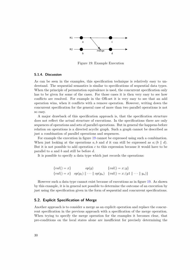
Figure 19: Example Execution
5.1.4. Discussion
As can be seen in the examples, this specification technique is relatively easy to un-derstand. The sequential semantics is similar to specifications of sequential data types.When the principle of permutation equivalence is used, the concurrent specification onlyhas to be given for some of the cases. For those cases it is then very easy to see howconflicts are resolved. For example in the OR-set it is very easy to see that an addoperation wins, when it conflicts with a remove operation. However, writing down theconcurrent specification for the general case of more than two parallel operations is notso easy.A major drawback of this specification approach is, that the specification structure
does not reflect the actual structure of executions. In the specifications there are onlysequences of operations and sets of parallel operations. But in general the happens-beforerelation on operations is a directed acyclic graph. Such a graph cannot be described asjust a combination of parallel operations and sequences.For example the execution in figure 19 cannot be expressed using such a combination.
When just looking at the operations a, b and d it can still be expressed as a; (b ‖ d).But it is not possible to add operation c to this expression because it would have to beparallel to a and b and still be before d.It is possible to specify a data type which just records the operations:
{val() = x} op(y) {val() = x; y}{val() = x} op(y1) ‖ · · · ‖ op(yn) {val() = x; (y1 ‖ · · · ‖ yn)}
However such a data type cannot exist because of executions as in figure 19. As shownby this example, it is in general not possible to determine the outcome of an execution byjust using the specification given in the form of sequential and concurrent specifications.
5.2. Explicit Specification of Merge
Another approach is to consider a merge as an explicit operation and replace the concur-rent specification in the previous approach with a specification of the merge operation.When trying to specify the merge operation for the examples it becomes clear, thatpre-conditions on the local states alone are insufficient for precisely determining the
30
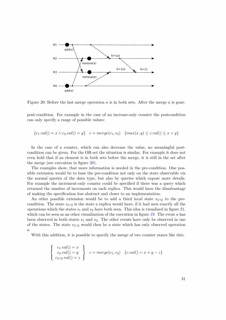
Figure 20: Before the last merge operation a is in both sets. After the merge a is gone.
post-condition. For example in the case of an increase-only counter the postconditioncan only specify a range of possible values:
{c1.val() = x ∧ c2.val() = y} c = merge(c1, c2) {max(x, y) ≤ c.val() ≤ x+ y}
In the case of a counter, which can also decrease the value, no meaningful post-condition can be given. For the OR-set the situation is similar. For example it does noteven hold that if an element is in both sets before the merge, it is still in the set afterthe merge (see execution in figure 20).The examples show, that more information is needed in the pre-condition. One pos-
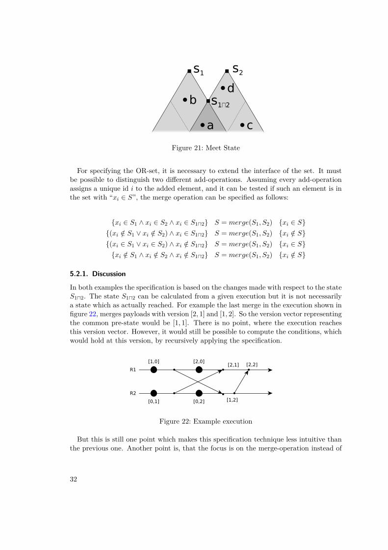
sible extension would be to base the pre-condition not only on the state observable viathe normal queries of the data type, but also by queries which expose more details.For example the increment-only counter could be specified if there was a query whichreturned the number of increments on each replica. This would have the disadvantageof making the specification less abstract and closer to an implementation.An other possible extension would be to add a third local state s1u2 to the pre-
condition. The state s1u2 is the state a replica would have, if it had seen exactly all theoperations which the states s1 and s2 have both seen. This idea is visualized in figure 21,which can be seen as an other visualization of the execution in figure 19. The event a hasbeen observed in both states s1 and s2. The other events have only be observed in oneof the states. The state s1u2 would then be a state which has only observed operationa.With this addition, it is possible to specify the merge of two counter states like this:
c1.val() = xc2.val() = yc1u2.val() = z
c = merge(c1, c2) {c.val() = x+ y − z}
31
s1 s2
s1⨅2b
a c
d
Figure 21: Meet State
For specifying the OR-set, it is necessary to extend the interface of the set. It mustbe possible to distinguish two different add-operations. Assuming every add-operationassigns a unique id i to the added element, and it can be tested if such an element is inthe set with “xi ∈ S”, the merge operation can be specified as follows:
{xi ∈ S1 ∧ xi ∈ S2 ∧ xi ∈ S1u2} S = merge(S1, S2) {xi ∈ S}{(xi /∈ S1 ∨ xi /∈ S2) ∧ xi ∈ S1u2} S = merge(S1, S2) {xi /∈ S}{(xi ∈ S1 ∨ xi ∈ S2) ∧ xi /∈ S1u2} S = merge(S1, S2) {xi ∈ S}{xi /∈ S1 ∧ xi /∈ S2 ∧ xi /∈ S1u2} S = merge(S1, S2) {xi /∈ S}
5.2.1. Discussion
In both examples the specification is based on the changes made with respect to the stateS1u2. The state S1u2 can be calculated from a given execution but it is not necessarilya state which as actually reached. For example the last merge in the execution shown infigure 22, merges payloads with version [2, 1] and [1, 2]. So the version vector representingthe common pre-state would be [1, 1]. There is no point, where the execution reachesthis version vector. However, it would still be possible to compute the conditions, whichwould hold at this version, by recursively applying the specification.
Figure 22: Example execution
But this is still one point which makes this specification technique less intuitive thanthe previous one. Another point is, that the focus is on the merge-operation instead of
32
the actual data type operations.The advantage of this approach is, that it allows to specify the behavior completely.
There are no executions where a specification of this kind cannot be applied.
5.3. Specification based on Update History
The update history of an execution is a tuple (E,≺), where E is the set of events inthe execution and ≺ is the happens-before relation between operations. An event has areplica on which it occurred and an update-operation. Merges are not an explicit partof the update history, but they influence the happens-before relation.The happens-before relation is a partial order. All events on the same replica are or-
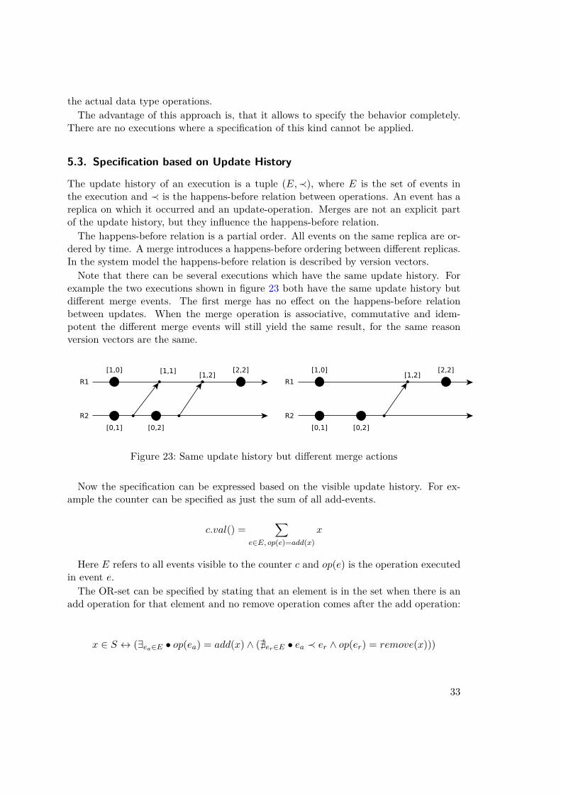
dered by time. A merge introduces a happens-before ordering between different replicas.In the system model the happens-before relation is described by version vectors.Note that there can be several executions which have the same update history. For
example the two executions shown in figure 23 both have the same update history butdifferent merge events. The first merge has no effect on the happens-before relationbetween updates. When the merge operation is associative, commutative and idem-potent the different merge events will still yield the same result, for the same reasonversion vectors are the same.
Figure 23: Same update history but different merge actions
Now the specification can be expressed based on the visible update history. For ex-ample the counter can be specified as just the sum of all add-events.
c.val() =∑
e∈E, op(e)=add(x)x
Here E refers to all events visible to the counter c and op(e) is the operation executedin event e.The OR-set can be specified by stating that an element is in the set when there is an
add operation for that element and no remove operation comes after the add operation:
x ∈ S ↔ (∃ea∈E • op(ea) = add(x) ∧ (@er∈E • ea ≺ er ∧ op(er) = remove(x)))
33
5.3.1. Discussion
This specification technique has a very straight-forward semantics. One can take anexecution, compute the events and happens-before relation and then apply the speci-fication. It would even be possible to generate a data type implementation from thespecification. The data type would store all the events and maintain a happens-beforerelation and the query functions would be equivalent to the specification.A disadvantage of this technique is, that it is based on the entire execution, whereas
the other techniques are better suited for reasoning about the effect of a single operationor a part of an execution when knowing the pre-state of the system. This might berelevant when using a CRDT specification to verify the behavior of an application usingCRDTs. For example an application could execute an update only after checking someconditions, so while the application code is not aware of the entire histories of the usedCRDT objects, it can know something about the state of the objects before executingthe updates.But while specifications based on pre-conditions might be better suited for verifying
applications, a specification which is based on the complete update history is a completespecification and so it should be possible to derive the validity of other specificationsfrom the validity of the former specification.For this reason I decided to use this kind of specification as the basis for describing
and verifying the behavior of CRDTs.
5.3.2. Realization in Isabelle
This section describes how the specification technique was formalized in Isabelle/HOL.First of all a type for the update history is required. As seen in the previous section,the update history has to capture all update operations and the happens-before relationbetween those operations. In a mathematical model this would usually be modeled asa tuple (E,≺), where E is the set of events (update-operations) and ≺ is the happens-before relation between events. And an event is then just a tuple (v, r, args), where v isthe version vector describing the time of the event, r is the replica-ID of the replica onwhich the operation was executed, and args are the arguments to the update function.The version v is a unique identifier for an event. If the event was just a tuple (r, args),then it would not be possible to distinguish two update operations with the same argu-ments on the same replica. The version vector also captures the happens-before relationbetween events, so it is only necessary to explicitly have a set E instead of the tuple(E,≺).When the events are stored in a set, hardly any properties of the update history are
reflected in the data structure and have to be expressed as additional constraints. Forexample the uniqueness of version vectors would be clear if the data structure for eventswas a map from versions to (r, args) tuples. When using a set this property has tobe captured elsewhere. So my first approach was to use a map for storing the events.However some other properties like the compatibility of update histories was not so nicewith this structure, as it does not reflect the concept of replicas very well. In many
34
type_synonym ’ua updateHistory = "replicaId ⇒ (versionVector × ’ua) list"
Figure 24: Update History Type
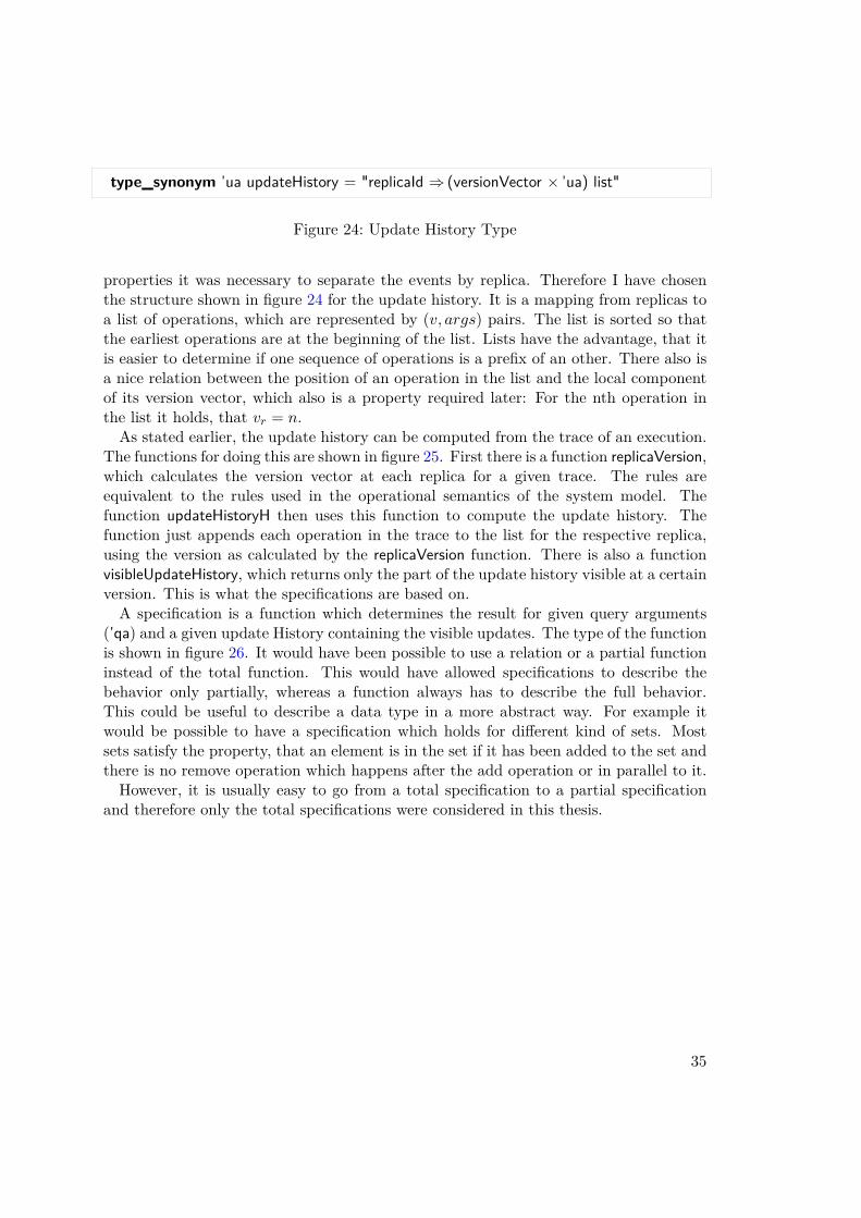
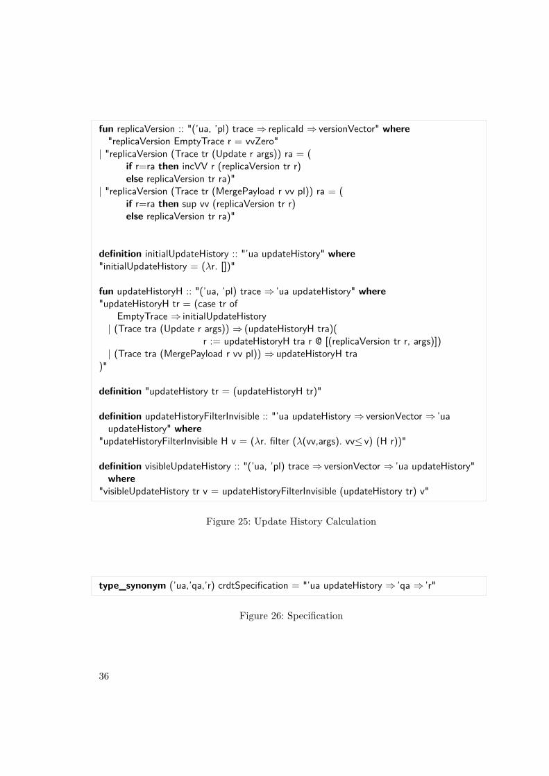
properties it was necessary to separate the events by replica. Therefore I have chosenthe structure shown in figure 24 for the update history. It is a mapping from replicas toa list of operations, which are represented by (v, args) pairs. The list is sorted so thatthe earliest operations are at the beginning of the list. Lists have the advantage, that itis easier to determine if one sequence of operations is a prefix of an other. There also isa nice relation between the position of an operation in the list and the local componentof its version vector, which also is a property required later: For the nth operation inthe list it holds, that vr = n.As stated earlier, the update history can be computed from the trace of an execution.
The functions for doing this are shown in figure 25. First there is a function replicaVersion,which calculates the version vector at each replica for a given trace. The rules areequivalent to the rules used in the operational semantics of the system model. Thefunction updateHistoryH then uses this function to compute the update history. Thefunction just appends each operation in the trace to the list for the respective replica,using the version as calculated by the replicaVersion function. There is also a functionvisibleUpdateHistory, which returns only the part of the update history visible at a certainversion. This is what the specifications are based on.A specification is a function which determines the result for given query arguments
(’qa) and a given update History containing the visible updates. The type of the functionis shown in figure 26. It would have been possible to use a relation or a partial functioninstead of the total function. This would have allowed specifications to describe thebehavior only partially, whereas a function always has to describe the full behavior.This could be useful to describe a data type in a more abstract way. For example itwould be possible to have a specification which holds for different kind of sets. Mostsets satisfy the property, that an element is in the set if it has been added to the set andthere is no remove operation which happens after the add operation or in parallel to it.However, it is usually easy to go from a total specification to a partial specification
and therefore only the total specifications were considered in this thesis.
35
fun replicaVersion :: "(’ua, ’pl) trace ⇒ replicaId ⇒ versionVector" where"replicaVersion EmptyTrace r = vvZero"
| "replicaVersion (Trace tr (Update r args)) ra = (if r=ra then incVV r (replicaVersion tr r)else replicaVersion tr ra)"
| "replicaVersion (Trace tr (MergePayload r vv pl)) ra = (if r=ra then sup vv (replicaVersion tr r)else replicaVersion tr ra)"
definition initialUpdateHistory :: "’ua updateHistory" where"initialUpdateHistory = (λr. [])"
fun updateHistoryH :: "(’ua, ’pl) trace ⇒ ’ua updateHistory" where"updateHistoryH tr = (case tr of
EmptyTrace ⇒ initialUpdateHistory| (Trace tra (Update r args)) ⇒ (updateHistoryH tra)(
r := updateHistoryH tra r @ [(replicaVersion tr r, args)])| (Trace tra (MergePayload r vv pl)) ⇒ updateHistoryH tra
)"
definition "updateHistory tr = (updateHistoryH tr)"
definition updateHistoryFilterInvisible :: "’ua updateHistory ⇒ versionVector ⇒ ’uaupdateHistory" where
"updateHistoryFilterInvisible H v = (λr. filter (λ(vv,args). vv≤ v) (H r))"
definition visibleUpdateHistory :: "(’ua, ’pl) trace ⇒ versionVector ⇒ ’ua updateHistory"where
"visibleUpdateHistory tr v = updateHistoryFilterInvisible (updateHistory tr) v"
Figure 25: Update History Calculation
type_synonym (’ua,’qa,’r) crdtSpecification = "’ua updateHistory ⇒ ’qa ⇒ ’r"
Figure 26: Specification
36
6. Verifying CRDT behavior
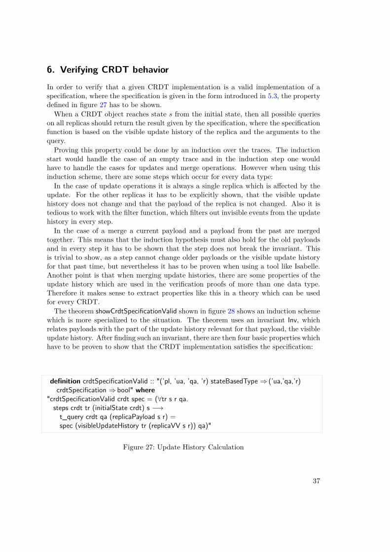
In order to verify that a given CRDT implementation is a valid implementation of aspecification, where the specification is given in the form introduced in 5.3, the propertydefined in figure 27 has to be shown.When a CRDT object reaches state s from the initial state, then all possible queries
on all replicas should return the result given by the specification, where the specificationfunction is based on the visible update history of the replica and the arguments to thequery.Proving this property could be done by an induction over the traces. The induction
start would handle the case of an empty trace and in the induction step one wouldhave to handle the cases for updates and merge operations. However when using thisinduction scheme, there are some steps which occur for every data type:In the case of update operations it is always a single replica which is affected by the
update. For the other replicas it has to be explicitly shown, that the visible updatehistory does not change and that the payload of the replica is not changed. Also it istedious to work with the filter function, which filters out invisible events from the updatehistory in every step.In the case of a merge a current payload and a payload from the past are merged
together. This means that the induction hypothesis must also hold for the old payloadsand in every step it has to be shown that the step does not break the invariant. Thisis trivial to show, as a step cannot change older payloads or the visible update historyfor that past time, but nevertheless it has to be proven when using a tool like Isabelle.Another point is that when merging update histories, there are some properties of theupdate history which are used in the verification proofs of more than one data type.Therefore it makes sense to extract properties like this in a theory which can be usedfor every CRDT.The theorem showCrdtSpecificationValid shown in figure 28 shows an induction scheme
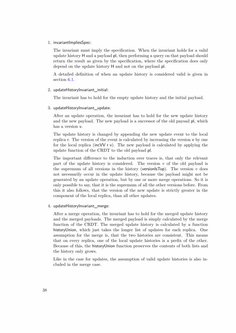
which is more specialized to the situation. The theorem uses an invariant Inv, whichrelates payloads with the part of the update history relevant for that payload, the visibleupdate history. After finding such an invariant, there are then four basic properties whichhave to be proven to show that the CRDT implementation satisfies the specification:
definition crdtSpecificationValid :: "(’pl, ’ua, ’qa, ’r) stateBasedType ⇒ (’ua,’qa,’r)crdtSpecification ⇒ bool" where
"crdtSpecificationValid crdt spec = (∀tr s r qa.steps crdt tr (initialState crdt) s −→t_query crdt qa (replicaPayload s r) =spec (visibleUpdateHistory tr (replicaVV s r)) qa)"
Figure 27: Update History Calculation
37
1. invariantImpliesSpec:
The invariant must imply the specification. When the invariant holds for a validupdate history H and a payload pl, then performing a query on that payload shouldreturn the result as given by the specification, where the specification does onlydepend on the update history H and not on the payload pl.
A detailed definition of when an update history is considered valid is given insection 6.1.
2. updateHistoryInvariant_initial:
The invariant has to hold for the empty update history and the initial payload.
3. updateHistoryInvariant_update:
After an update operation, the invariant has to hold for the new update historyand the new payload. The new payload is a successor of the old payoad pl, whichhas a version v.
The update history is changed by appending the new update event to the localreplica r. The version of the event is calculated by increasing the version v by onefor the local replica (incVV r v). The new payload is calculated by applying theupdate function of the CRDT to the old payload pl.
The important difference to the induction over traces is, that only the relevantpart of the update history is considered. The version v of the old payload isthe supremum of all versions in the history (versionIsTop). The version v doesnot necessarily occur in the update history, because the payload might not begenerated by an update operation, but by one or more merge operations. So it isonly possible to say, that it is the supremum of all the other versions before. Fromthis it also follows, that the version of the new update is strictly greater in thecomponent of the local replica, than all other updates.
4. updateHistoryInvariant_merge:
After a merge operation, the invariant has to hold for the merged update historyand the merged payloads. The merged payload is simply calculated by the mergefunction of the CRDT. The merged update history is calculated by a functionhistoryUnion, which just takes the longer list of updates for each replica. Oneassumption for the merge is, that the two histories are consistent. This meansthat on every replica, one of the local update histories is a prefix of the other.Because of this, the historyUnion function preserves the contents of both lists andthe history only grows.
Like in the case for updates, the assumption of valid update histories is also in-cluded in the merge case.
38
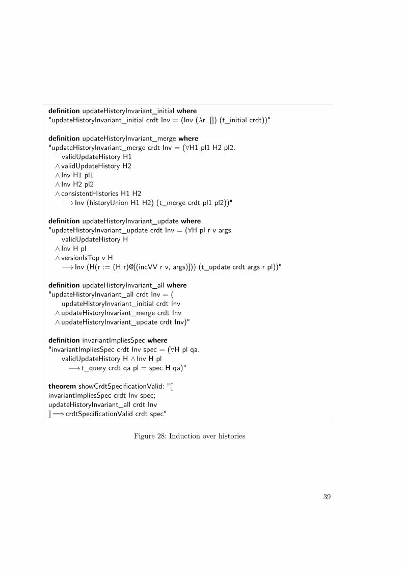
definition updateHistoryInvariant_initial where"updateHistoryInvariant_initial crdt Inv = (Inv (λr. []) (t_initial crdt))"
definition updateHistoryInvariant_merge where"updateHistoryInvariant_merge crdt Inv = (∀H1 pl1 H2 pl2.
validUpdateHistory H1∧ validUpdateHistory H2∧ Inv H1 pl1∧ Inv H2 pl2∧ consistentHistories H1 H2−→ Inv (historyUnion H1 H2) (t_merge crdt pl1 pl2))"
definition updateHistoryInvariant_update where"updateHistoryInvariant_update crdt Inv = (∀H pl r v args.
validUpdateHistory H∧ Inv H pl∧ versionIsTop v H−→ Inv (H(r := (H r)@[(incVV r v, args)])) (t_update crdt args r pl))"
definition updateHistoryInvariant_all where"updateHistoryInvariant_all crdt Inv = (
updateHistoryInvariant_initial crdt Inv∧ updateHistoryInvariant_merge crdt Inv∧ updateHistoryInvariant_update crdt Inv)"
definition invariantImpliesSpec where"invariantImpliesSpec crdt Inv spec = (∀H pl qa.
validUpdateHistory H ∧ Inv H pl−→ t_query crdt qa pl = spec H qa)"
theorem showCrdtSpecificationValid: "JinvariantImpliesSpec crdt Inv spec;updateHistoryInvariant_all crdt InvK =⇒ crdtSpecificationValid crdt spec"
Figure 28: Induction over histories
39
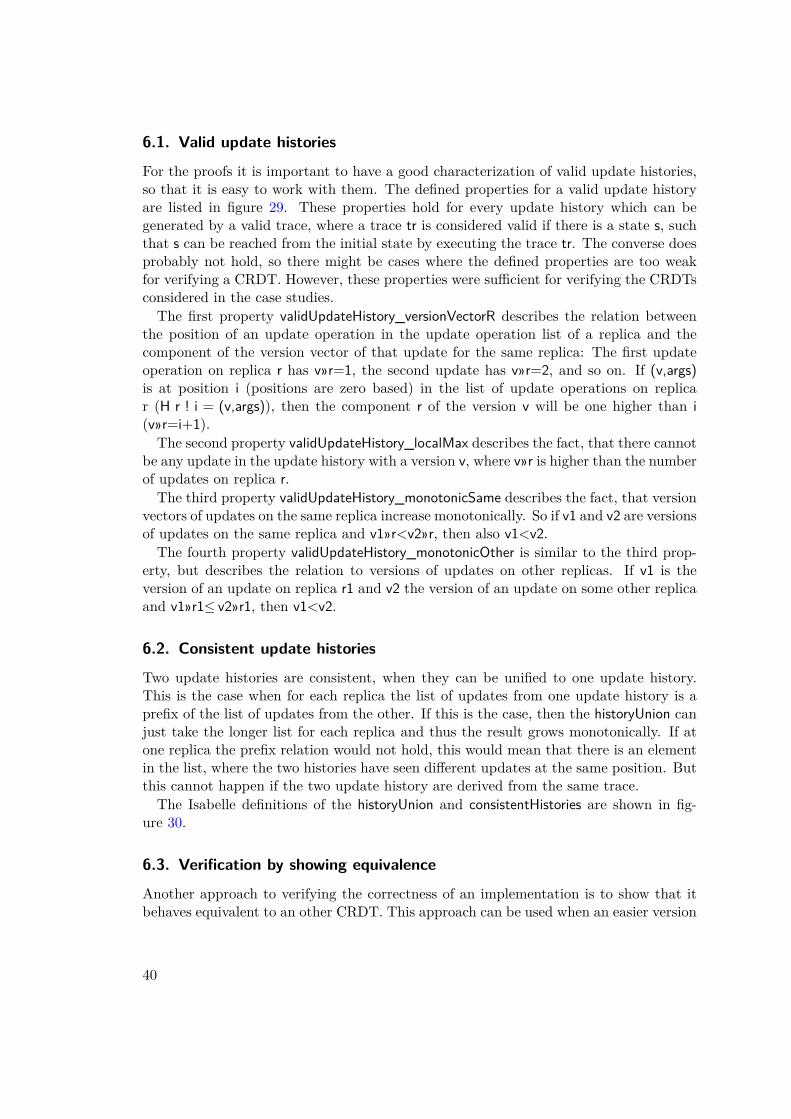
6.1. Valid update histories
For the proofs it is important to have a good characterization of valid update histories,so that it is easy to work with them. The defined properties for a valid update historyare listed in figure 29. These properties hold for every update history which can begenerated by a valid trace, where a trace tr is considered valid if there is a state s, suchthat s can be reached from the initial state by executing the trace tr. The converse doesprobably not hold, so there might be cases where the defined properties are too weakfor verifying a CRDT. However, these properties were sufficient for verifying the CRDTsconsidered in the case studies.The first property validUpdateHistory_versionVectorR describes the relation between
the position of an update operation in the update operation list of a replica and thecomponent of the version vector of that update for the same replica: The first updateoperation on replica r has v»r=1, the second update has v»r=2, and so on. If (v,args)is at position i (positions are zero based) in the list of update operations on replicar (H r ! i = (v,args)), then the component r of the version v will be one higher than i(v»r=i+1).The second property validUpdateHistory_localMax describes the fact, that there cannot
be any update in the update history with a version v, where v»r is higher than the numberof updates on replica r.The third property validUpdateHistory_monotonicSame describes the fact, that version
vectors of updates on the same replica increase monotonically. So if v1 and v2 are versionsof updates on the same replica and v1»r<v2»r, then also v1<v2.The fourth property validUpdateHistory_monotonicOther is similar to the third prop-
erty, but describes the relation to versions of updates on other replicas. If v1 is theversion of an update on replica r1 and v2 the version of an update on some other replicaand v1»r1≤ v2»r1, then v1<v2.
6.2. Consistent update histories
Two update histories are consistent, when they can be unified to one update history.This is the case when for each replica the list of updates from one update history is aprefix of the list of updates from the other. If this is the case, then the historyUnion canjust take the longer list for each replica and thus the result grows monotonically. If atone replica the prefix relation would not hold, this would mean that there is an elementin the list, where the two histories have seen different updates at the same position. Butthis cannot happen if the two update history are derived from the same trace.The Isabelle definitions of the historyUnion and consistentHistories are shown in fig-
ure 30.
6.3. Verification by showing equivalence
Another approach to verifying the correctness of an implementation is to show that itbehaves equivalent to an other CRDT. This approach can be used when an easier version
40
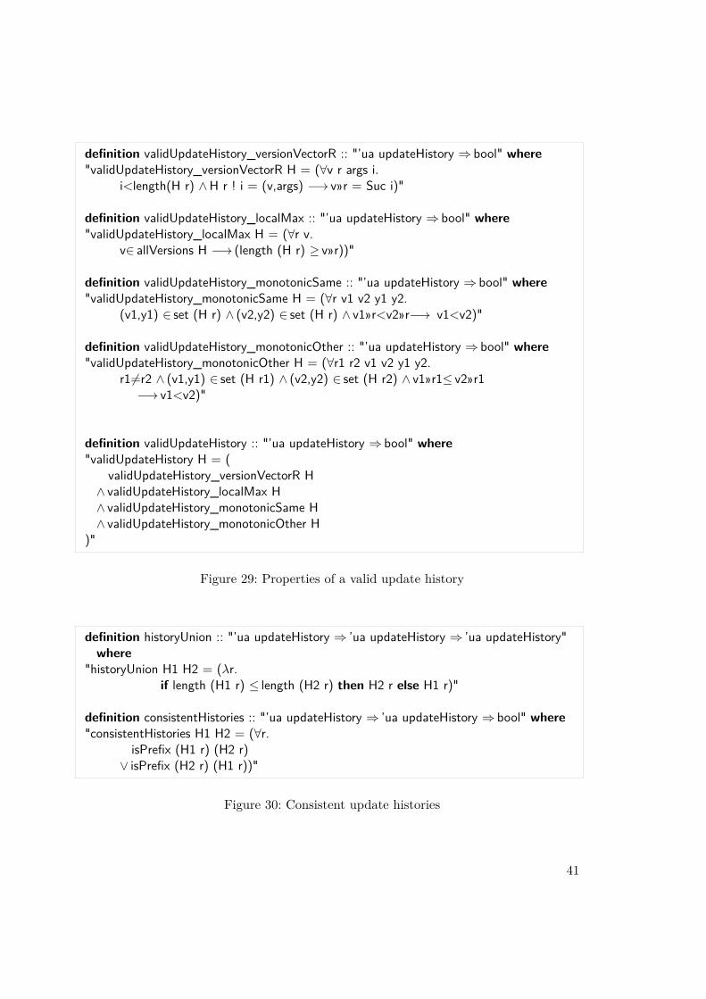
definition validUpdateHistory_versionVectorR :: "’ua updateHistory ⇒ bool" where"validUpdateHistory_versionVectorR H = (∀v r args i.
i<length(H r) ∧H r ! i = (v,args) −→ v»r = Suc i)"
definition validUpdateHistory_localMax :: "’ua updateHistory ⇒ bool" where"validUpdateHistory_localMax H = (∀r v.
v∈ allVersions H −→ (length (H r) ≥ v»r))"
definition validUpdateHistory_monotonicSame :: "’ua updateHistory ⇒ bool" where"validUpdateHistory_monotonicSame H = (∀r v1 v2 y1 y2.
(v1,y1) ∈ set (H r) ∧ (v2,y2) ∈ set (H r) ∧ v1»r<v2»r−→ v1<v2)"
definition validUpdateHistory_monotonicOther :: "’ua updateHistory ⇒ bool" where"validUpdateHistory_monotonicOther H = (∀r1 r2 v1 v2 y1 y2.
r16=r2 ∧ (v1,y1) ∈ set (H r1) ∧ (v2,y2) ∈ set (H r2) ∧ v1»r1≤ v2»r1−→ v1<v2)"
definition validUpdateHistory :: "’ua updateHistory ⇒ bool" where"validUpdateHistory H = (
validUpdateHistory_versionVectorR H∧ validUpdateHistory_localMax H∧ validUpdateHistory_monotonicSame H∧ validUpdateHistory_monotonicOther H
)"
Figure 29: Properties of a valid update history
definition historyUnion :: "’ua updateHistory ⇒ ’ua updateHistory ⇒ ’ua updateHistory"where
"historyUnion H1 H2 = (λr.if length (H1 r) ≤ length (H2 r) then H2 r else H1 r)"
definition consistentHistories :: "’ua updateHistory ⇒ ’ua updateHistory ⇒ bool" where"consistentHistories H1 H2 = (∀r.
isPrefix (H1 r) (H2 r)∨ isPrefix (H2 r) (H1 r))"
Figure 30: Consistent update histories
41
of a CRDT is already verified and an optimized version of the CRDT behaves in a similarway. Behaving in a similar way means, that it is possible to define a coupling betweenthe payloads of the two CRDTs. The properties of this coupling are shown in figure 31.The coupling must hold in the initial state and it must be preserved by update andmerge operations, and for two coupled payloads, the same query must return the sameresult.The theorem simulation in figure 31 states that when an crdtA fulfills a specification
spec and there is a coupling between crdtA and crdtB, then crdtB also fulfills the samespecification. This theorem can be proven by an induction over the traces for crdtA.Because the traces include the payloads in the merge actions, traces for crdtA are notapplicable for crdtB, but there always exists an equivalent trace where the payloads inthe trace are replaced with coupled payloads.The idea of simulation could probably be expanded to more than one CRDT. For
example a PN-counter could be simulated by two increase-only-counters. This couldmake it easier to verify CRDTs which are compositions of other CRDTs. Because oftime constraints this approach was not examined further.
42
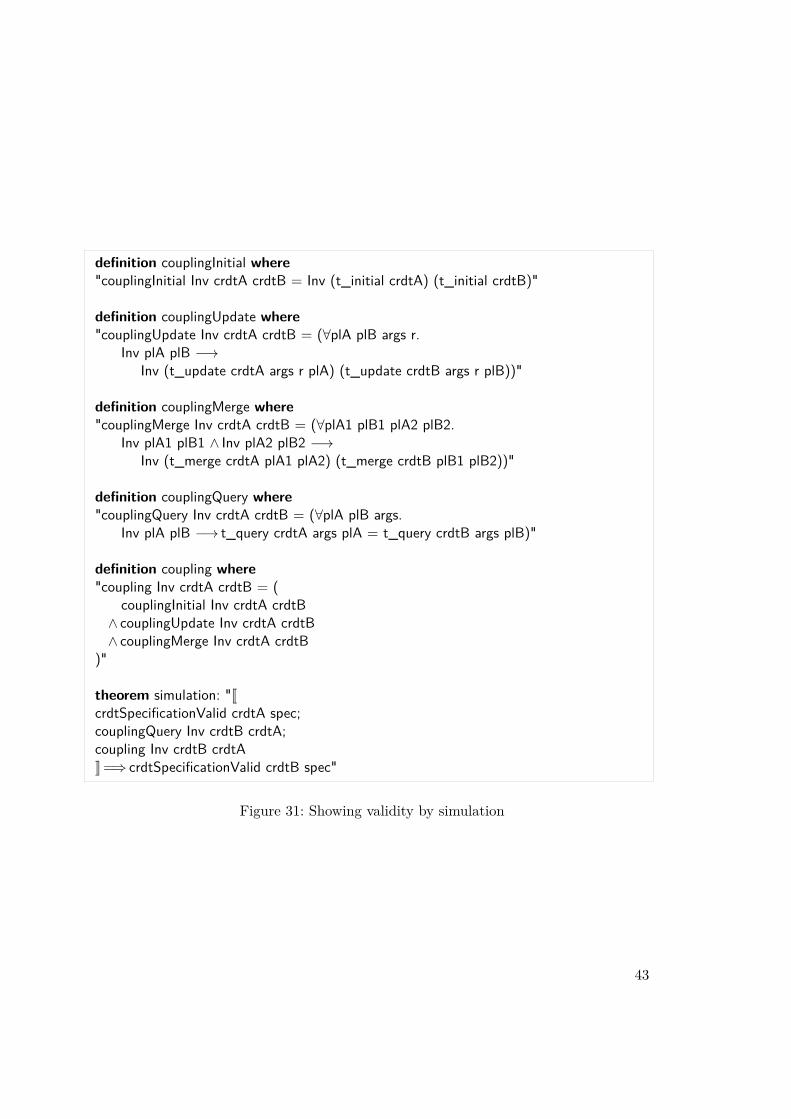
definition couplingInitial where"couplingInitial Inv crdtA crdtB = Inv (t_initial crdtA) (t_initial crdtB)"
definition couplingUpdate where"couplingUpdate Inv crdtA crdtB = (∀plA plB args r.
Inv plA plB −→Inv (t_update crdtA args r plA) (t_update crdtB args r plB))"
definition couplingMerge where"couplingMerge Inv crdtA crdtB = (∀plA1 plB1 plA2 plB2.
Inv plA1 plB1 ∧ Inv plA2 plB2 −→Inv (t_merge crdtA plA1 plA2) (t_merge crdtB plB1 plB2))"
definition couplingQuery where"couplingQuery Inv crdtA crdtB = (∀plA plB args.
Inv plA plB −→ t_query crdtA args plA = t_query crdtB args plB)"
definition coupling where"coupling Inv crdtA crdtB = (
couplingInitial Inv crdtA crdtB∧ couplingUpdate Inv crdtA crdtB∧ couplingMerge Inv crdtA crdtB
)"
theorem simulation: "JcrdtSpecificationValid crdtA spec;couplingQuery Inv crdtB crdtA;coupling Inv crdtB crdtAK =⇒ crdtSpecificationValid crdtB spec"
Figure 31: Showing validity by simulation
43

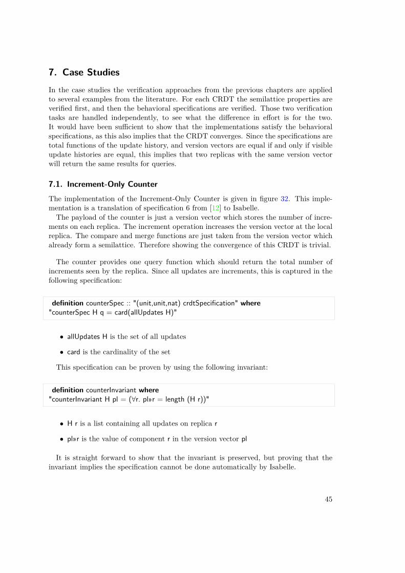
7. Case StudiesIn the case studies the verification approaches from the previous chapters are appliedto several examples from the literature. For each CRDT the semilattice properties areverified first, and then the behavioral specifications are verified. Those two verificationtasks are handled independently, to see what the difference in effort is for the two.It would have been sufficient to show that the implementations satisfy the behavioralspecifications, as this also implies that the CRDT converges. Since the specifications aretotal functions of the update history, and version vectors are equal if and only if visibleupdate histories are equal, this implies that two replicas with the same version vectorwill return the same results for queries.
7.1. Increment-Only Counter
The implementation of the Increment-Only Counter is given in figure 32. This imple-mentation is a translation of specification 6 from [12] to Isabelle.The payload of the counter is just a version vector which stores the number of incre-
ments on each replica. The increment operation increases the version vector at the localreplica. The compare and merge functions are just taken from the version vector whichalready form a semilattice. Therefore showing the convergence of this CRDT is trivial.
The counter provides one query function which should return the total number ofincrements seen by the replica. Since all updates are increments, this is captured in thefollowing specification:
definition counterSpec :: "(unit,unit,nat) crdtSpecification" where"counterSpec H q = card(allUpdates H)"
• allUpdates H is the set of all updates
• card is the cardinality of the set
This specification can be proven by using the following invariant:
definition counterInvariant where"counterInvariant H pl = (∀r. pl»r = length (H r))"
• H r is a list containing all updates on replica r
• pl»r is the value of component r in the version vector pl
It is straight forward to show that the invariant is preserved, but proving that theinvariant implies the specification cannot be done automatically by Isabelle.
45
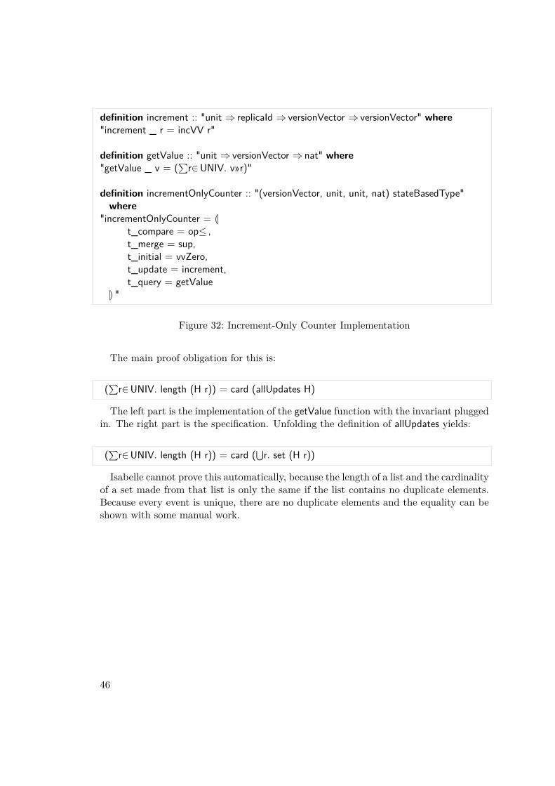
definition increment :: "unit ⇒ replicaId ⇒ versionVector ⇒ versionVector" where"increment _ r = incVV r"
definition getValue :: "unit ⇒ versionVector ⇒ nat" where"getValue _ v = (
∑r∈UNIV. v»r)"
definition incrementOnlyCounter :: "(versionVector, unit, unit, nat) stateBasedType"where
"incrementOnlyCounter = Lt_compare = op≤ ,t_merge = sup,t_initial = vvZero,t_update = increment,t_query = getValue
M "
Figure 32: Increment-Only Counter Implementation
The main proof obligation for this is:
(∑r∈UNIV. length (H r)) = card (allUpdates H)
The left part is the implementation of the getValue function with the invariant pluggedin. The right part is the specification. Unfolding the definition of allUpdates yields:
(∑r∈UNIV. length (H r)) = card (
⋃r. set (H r))
Isabelle cannot prove this automatically, because the length of a list and the cardinalityof a set made from that list is only the same if the list contains no duplicate elements.Because every event is unique, there are no duplicate elements and the equality can beshown with some manual work.
46
7.2. PN-CounterThe PN-Counter is a counter which also allows decrementing its value. The implemen-tation in figure 33 is based on specification 7 in [12], but instead of having separateincrement and decrement functions there is only one update function which takes aninteger value.The payload is basically a pair of version vectors, but to avoid conversions between
natural numbers and integers, the version vector type was not used. Instead the payloaduses a function from replicaIds to integers.The first component of the payload counts the positive updates and the second com-
ponent counts the negative updates. Splitting the updates like this is essential for havingmonotonic updates and thus convergence.Proving that this CRDT forms a semilattice is relatively simple. No invariant is
required for the payload. Replacing the natural numbers with integers in the payloadhad no influence on the semilattice properties. But choosing a normal function typeinstead of the version vector type led to some additional steps in the proof.Figure 34 shows the specification of the PN-counter and the invariant to prove it
correct. The value of the counter is just the sum of the update arguments of all events.The invariant captures the splitting of events in a group of positive and a group ofnegative updates.The proof is similar to the increment-only case. The main problem is in showing that
the invariant implies the specification. This requires rewriting of some sums over sets tosums over lists, which requires some manual steps in Isabelle.
47
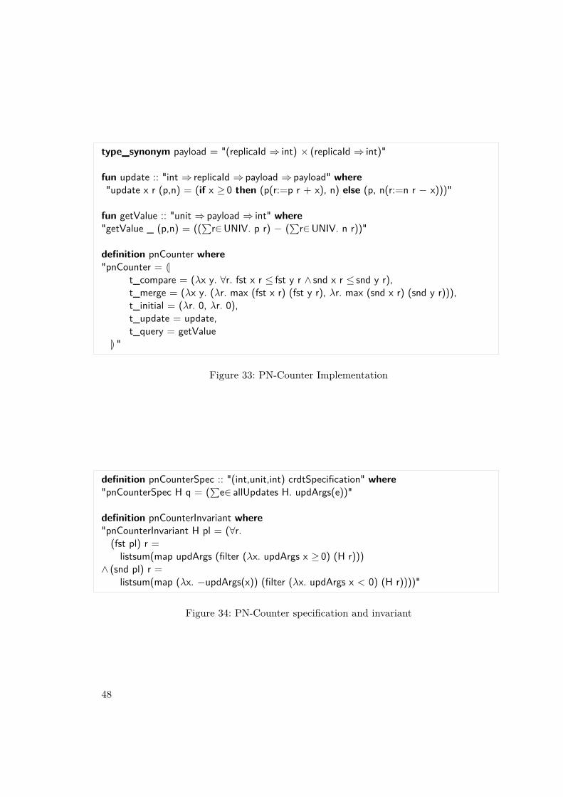
type_synonym payload = "(replicaId ⇒ int) × (replicaId ⇒ int)"
fun update :: "int ⇒ replicaId ⇒ payload ⇒ payload" where"update x r (p,n) = (if x ≥ 0 then (p(r:=p r + x), n) else (p, n(r:=n r − x)))"
fun getValue :: "unit ⇒ payload ⇒ int" where"getValue _ (p,n) = ((
∑r∈UNIV. p r) − (
∑r∈UNIV. n r))"
definition pnCounter where"pnCounter = L
t_compare = (λx y. ∀r. fst x r ≤ fst y r ∧ snd x r ≤ snd y r),t_merge = (λx y. (λr. max (fst x r) (fst y r), λr. max (snd x r) (snd y r))),t_initial = (λr. 0, λr. 0),t_update = update,t_query = getValue
M "
Figure 33: PN-Counter Implementation
definition pnCounterSpec :: "(int,unit,int) crdtSpecification" where"pnCounterSpec H q = (
∑e∈ allUpdates H. updArgs(e))"
definition pnCounterInvariant where"pnCounterInvariant H pl = (∀r.(fst pl) r =listsum(map updArgs (filter (λx. updArgs x ≥ 0) (H r)))
∧ (snd pl) r =listsum(map (λx. −updArgs(x)) (filter (λx. updArgs x < 0) (H r))))"
Figure 34: PN-Counter specification and invariant
48
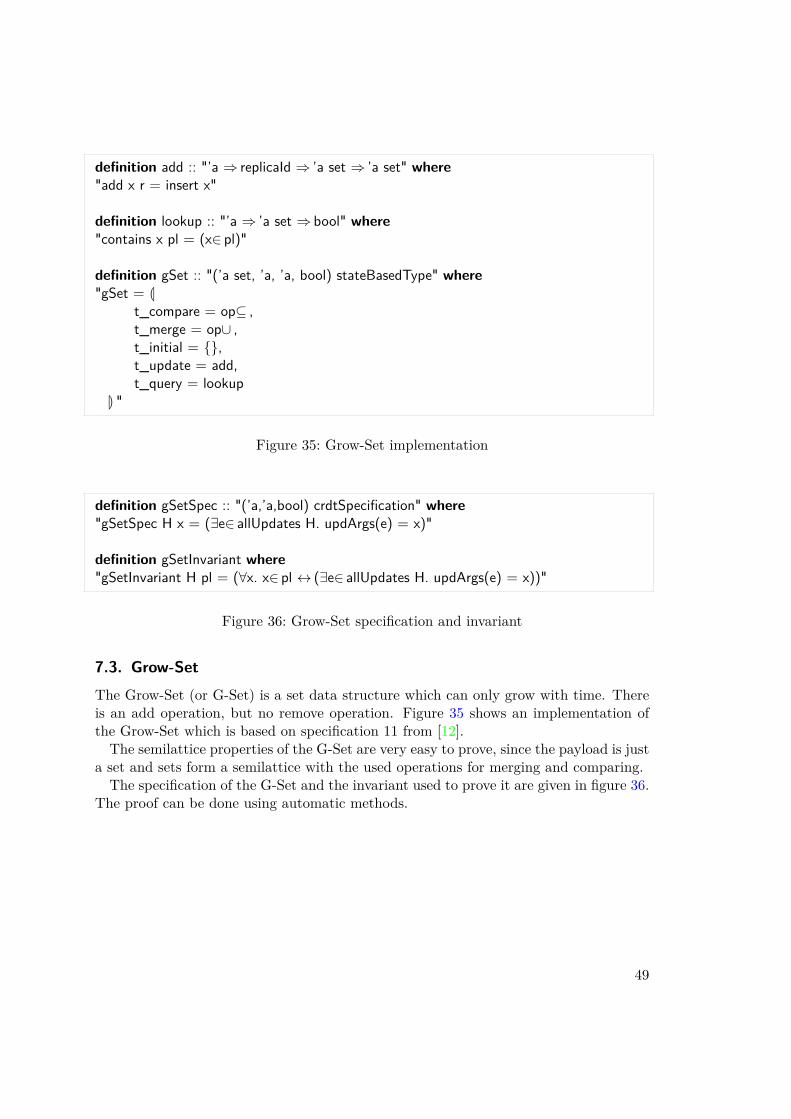
definition add :: "’a ⇒ replicaId ⇒ ’a set ⇒ ’a set" where"add x r = insert x"
definition lookup :: "’a ⇒ ’a set ⇒ bool" where"contains x pl = (x∈ pl)"
definition gSet :: "(’a set, ’a, ’a, bool) stateBasedType" where"gSet = L
t_compare = op⊆ ,t_merge = op∪ ,t_initial = {},t_update = add,t_query = lookup
M "
Figure 35: Grow-Set implementation
definition gSetSpec :: "(’a,’a,bool) crdtSpecification" where"gSetSpec H x = (∃e∈ allUpdates H. updArgs(e) = x)"
definition gSetInvariant where"gSetInvariant H pl = (∀x. x∈ pl ↔ (∃e∈ allUpdates H. updArgs(e) = x))"
Figure 36: Grow-Set specification and invariant
7.3. Grow-SetThe Grow-Set (or G-Set) is a set data structure which can only grow with time. Thereis an add operation, but no remove operation. Figure 35 shows an implementation ofthe Grow-Set which is based on specification 11 from [12].The semilattice properties of the G-Set are very easy to prove, since the payload is just
a set and sets form a semilattice with the used operations for merging and comparing.The specification of the G-Set and the invariant used to prove it are given in figure 36.
The proof can be done using automatic methods.
49
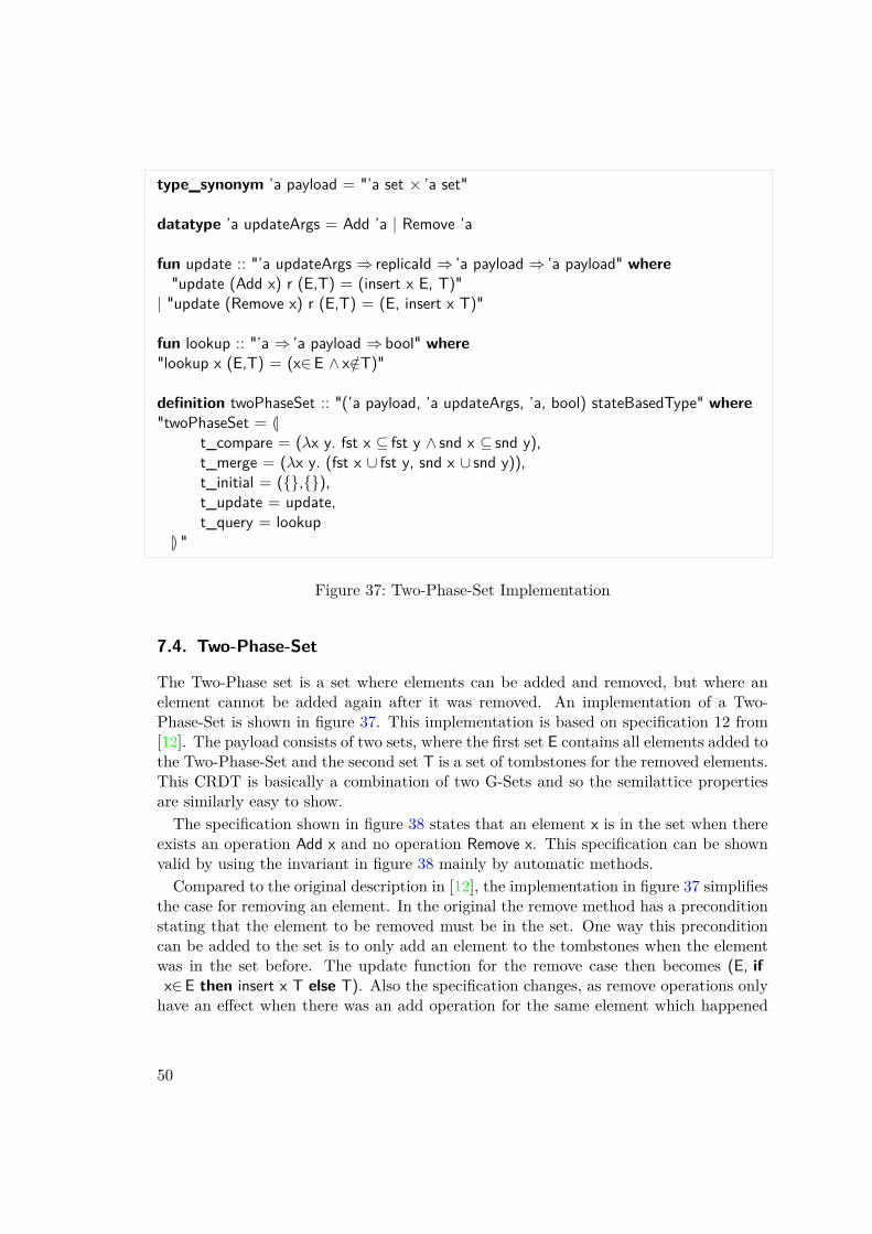
type_synonym ’a payload = "’a set × ’a set"
datatype ’a updateArgs = Add ’a | Remove ’a
fun update :: "’a updateArgs ⇒ replicaId ⇒ ’a payload ⇒ ’a payload" where"update (Add x) r (E,T) = (insert x E, T)"
| "update (Remove x) r (E,T) = (E, insert x T)"
fun lookup :: "’a ⇒ ’a payload ⇒ bool" where"lookup x (E,T) = (x∈E ∧ x/∈T)"
definition twoPhaseSet :: "(’a payload, ’a updateArgs, ’a, bool) stateBasedType" where"twoPhaseSet = L
t_compare = (λx y. fst x ⊆ fst y ∧ snd x ⊆ snd y),t_merge = (λx y. (fst x ∪ fst y, snd x ∪ snd y)),t_initial = ({},{}),t_update = update,t_query = lookup
M "
Figure 37: Two-Phase-Set Implementation
7.4. Two-Phase-Set
The Two-Phase set is a set where elements can be added and removed, but where anelement cannot be added again after it was removed. An implementation of a Two-Phase-Set is shown in figure 37. This implementation is based on specification 12 from[12]. The payload consists of two sets, where the first set E contains all elements added tothe Two-Phase-Set and the second set T is a set of tombstones for the removed elements.This CRDT is basically a combination of two G-Sets and so the semilattice propertiesare similarly easy to show.The specification shown in figure 38 states that an element x is in the set when there
exists an operation Add x and no operation Remove x. This specification can be shownvalid by using the invariant in figure 38 mainly by automatic methods.Compared to the original description in [12], the implementation in figure 37 simplifies
the case for removing an element. In the original the remove method has a preconditionstating that the element to be removed must be in the set. One way this preconditioncan be added to the set is to only add an element to the tombstones when the elementwas in the set before. The update function for the remove case then becomes (E, ifx∈E then insert x T else T). Also the specification changes, as remove operations onlyhave an effect when there was an add operation for the same element which happened
50
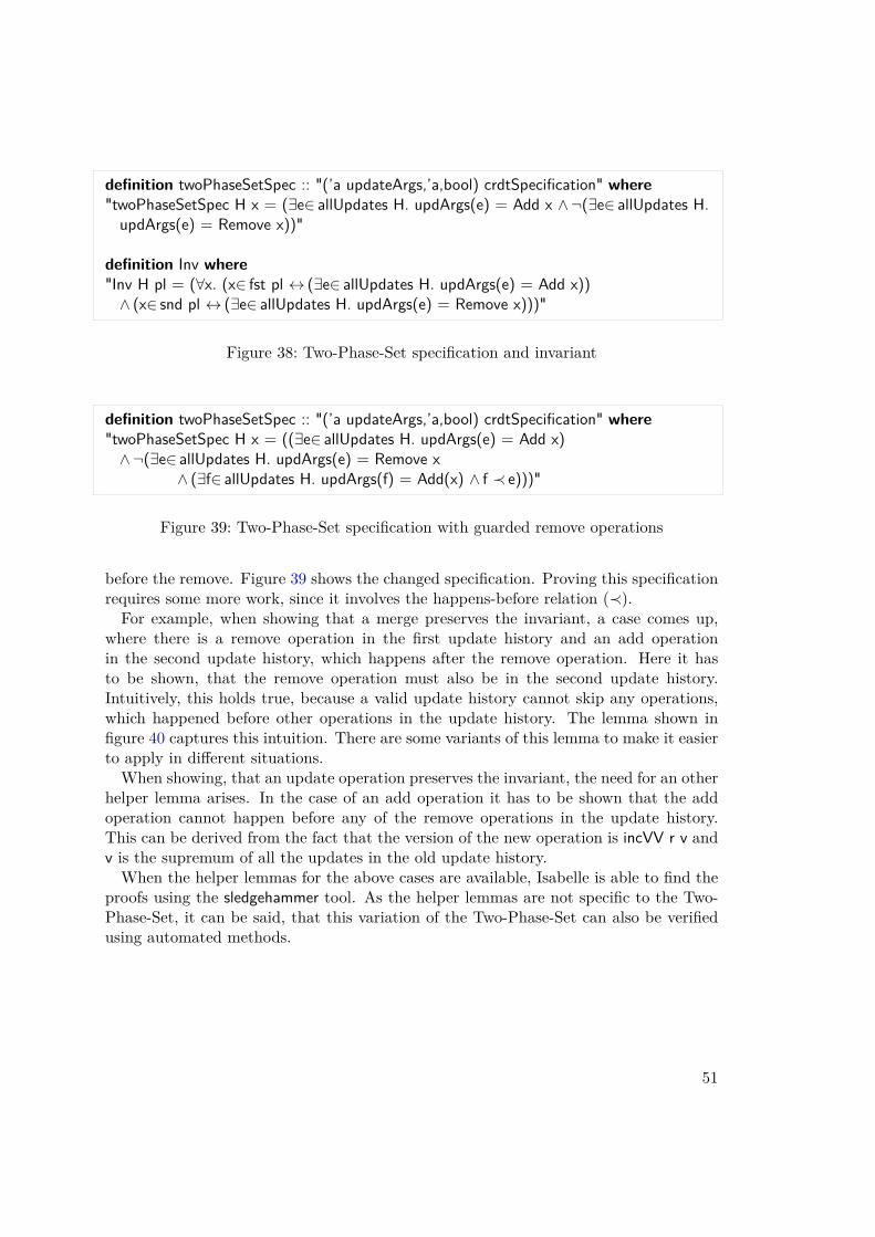
definition twoPhaseSetSpec :: "(’a updateArgs,’a,bool) crdtSpecification" where"twoPhaseSetSpec H x = (∃e∈ allUpdates H. updArgs(e) = Add x ∧¬(∃e∈ allUpdates H.updArgs(e) = Remove x))"
definition Inv where"Inv H pl = (∀x. (x∈ fst pl ↔ (∃e∈ allUpdates H. updArgs(e) = Add x))∧ (x∈ snd pl ↔ (∃e∈ allUpdates H. updArgs(e) = Remove x)))"
Figure 38: Two-Phase-Set specification and invariant
definition twoPhaseSetSpec :: "(’a updateArgs,’a,bool) crdtSpecification" where"twoPhaseSetSpec H x = ((∃e∈ allUpdates H. updArgs(e) = Add x)∧¬(∃e∈ allUpdates H. updArgs(e) = Remove x
∧ (∃f∈ allUpdates H. updArgs(f) = Add(x) ∧ f ≺ e)))"
Figure 39: Two-Phase-Set specification with guarded remove operations
before the remove. Figure 39 shows the changed specification. Proving this specificationrequires some more work, since it involves the happens-before relation (≺).For example, when showing that a merge preserves the invariant, a case comes up,
where there is a remove operation in the first update history and an add operationin the second update history, which happens after the remove operation. Here it hasto be shown, that the remove operation must also be in the second update history.Intuitively, this holds true, because a valid update history cannot skip any operations,which happened before other operations in the update history. The lemma shown infigure 40 captures this intuition. There are some variants of this lemma to make it easierto apply in different situations.When showing, that an update operation preserves the invariant, the need for an other
helper lemma arises. In the case of an add operation it has to be shown that the addoperation cannot happen before any of the remove operations in the update history.This can be derived from the fact that the version of the new operation is incVV r v andv is the supremum of all the updates in the old update history.When the helper lemmas for the above cases are available, Isabelle is able to find the
proofs using the sledgehammer tool. As the helper lemmas are not specific to the Two-Phase-Set, it can be said, that this variation of the Two-Phase-Set can also be verifiedusing automated methods.
51
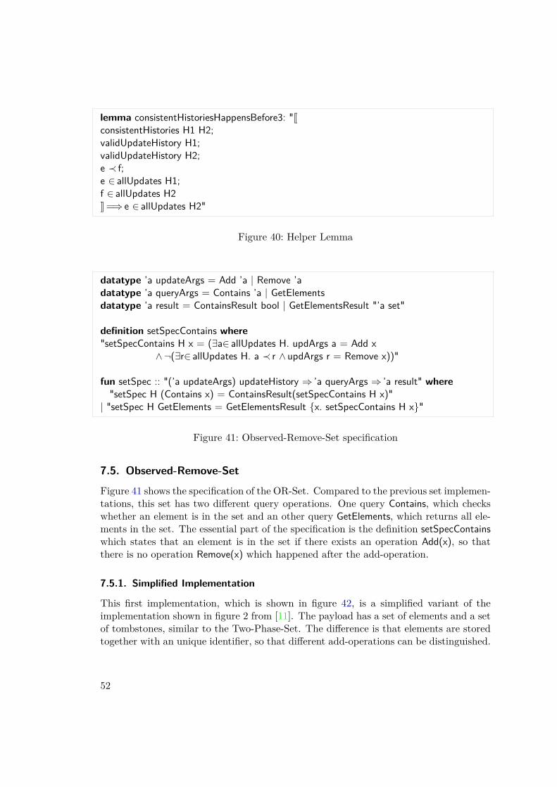
lemma consistentHistoriesHappensBefore3: "JconsistentHistories H1 H2;validUpdateHistory H1;validUpdateHistory H2;e ≺ f;e ∈ allUpdates H1;f ∈ allUpdates H2K =⇒ e ∈ allUpdates H2"
Figure 40: Helper Lemma
datatype ’a updateArgs = Add ’a | Remove ’adatatype ’a queryArgs = Contains ’a | GetElementsdatatype ’a result = ContainsResult bool | GetElementsResult "’a set"
definition setSpecContains where"setSpecContains H x = (∃a∈ allUpdates H. updArgs a = Add x
∧¬(∃r∈ allUpdates H. a ≺ r ∧ updArgs r = Remove x))"
fun setSpec :: "(’a updateArgs) updateHistory ⇒ ’a queryArgs ⇒ ’a result" where"setSpec H (Contains x) = ContainsResult(setSpecContains H x)"
| "setSpec H GetElements = GetElementsResult {x. setSpecContains H x}"
Figure 41: Observed-Remove-Set specification
7.5. Observed-Remove-Set
Figure 41 shows the specification of the OR-Set. Compared to the previous set implemen-tations, this set has two different query operations. One query Contains, which checkswhether an element is in the set and an other query GetElements, which returns all ele-ments in the set. The essential part of the specification is the definition setSpecContainswhich states that an element is in the set if there exists an operation Add(x), so thatthere is no operation Remove(x) which happened after the add-operation.
7.5.1. Simplified Implementation
This first implementation, which is shown in figure 42, is a simplified variant of theimplementation shown in figure 2 from [11]. The payload has a set of elements and a setof tombstones, similar to the Two-Phase-Set. The difference is that elements are storedtogether with an unique identifier, so that different add-operations can be distinguished.
52
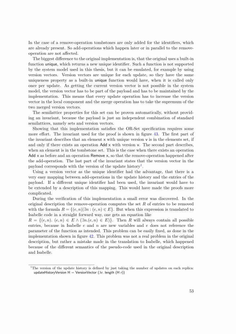
In the case of a remove-operation tombstones are only added for the identifiers, whichare already present. So add-operations which happen later or in parallel to the remove-operation are not affected.The biggest difference to the original implementation is, that the original uses a built-in
function unique, which returns a new unique identifier. Such a function is not supportedby the system model used in this thesis, but it can be emulated, for example by usingversion vectors. Version vectors are unique for each update, so they have the sameuniqueness property as a built-in unique function would have, when it is called onlyonce per update. As getting the current version vector is not possible in the systemmodel, the version vector has to be part of the payload and has to be maintained by theimplementation. This means that every update operation has to increase the versionvector in the local component and the merge operation has to take the supremum of thetwo merged version vectors.The semilattice properties for this set can be proven automatically, without provid-
ing an invariant, because the payload is just an independent combination of standardsemilattices, namely sets and version vectors.Showing that this implementation satisfies the OR-Set specification requires some
more effort. The invariant used for the proof is shown in figure 43. The first part ofthe invariant describes that an element x with unique version v is in the elements set, ifand only if there exists an operation Add x with version v. The second part describes,when an element is in the tombstone set. This is the case when there exists an operationAdd x as before and an operation Remove x, so that the remove-operation happened afterthe add-operation. The last part of the invariant states that the version vector in thepayload corresponds with the version of the update history1.Using a version vector as the unique identifier had the advantage, that there is a
very easy mapping between add-operations in the update history and the entries of thepayload. If a different unique identifier had been used, the invariant would have tobe extended by a description of this mapping. This would have made the proofs morecomplicated.During the verification of this implementation a small error was discovered. In the
original description the remove-operation computes the set R of entries to be removedwith the formula R = {(e, n)|∃n : (e, n) ∈ E}. But when this expression is translated toIsabelle code in a straight forward way, one gets an equation likeR = {(e, n). (e, n) ∈ E ∧ (∃n.(e, n) ∈ E)}. Then R will always contain all possibleentries, because in Isabelle e and n are new variables and e does not reference theparameter of the function as intended. This problem can be easily fixed, as done in theimplementation shown in figure 42. This problem was not a real problem in the originaldescription, but rather a mistake made in the translation to Isabelle, which happenedbecause of the different semantics of the pseudo-code used in the original descriptionand Isabelle.
1The version of the update history is defined by just taking the number of updates on each replica:updateHistoryVersion H = VersionVector (λr. length (H r))
53
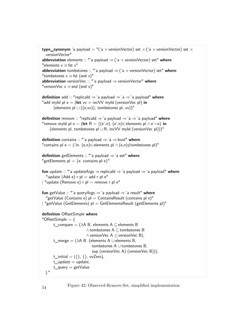
type_synonym ’a payload = "(’a × versionVector) set × (’a × versionVector) set ×versionVector"
abbreviation elements :: "’a payload ⇒ (’a × versionVector) set" where"elements x ≡ fst x"abbreviation tombstones :: "’a payload ⇒ (’a × versionVector) set" where"tombstones x ≡ fst (snd x)"abbreviation versionVec :: "’a payload ⇒ versionVector" where"versionVec x ≡ snd (snd x)"
definition add :: "replicaId ⇒ ’a payload ⇒ ’a ⇒ ’a payload" where"add myId pl e = (let vv = incVV myId (versionVec pl) in
(elements pl ∪ {(e,vv)}, tombstones pl, vv))"
definition remove :: "replicaId ⇒ ’a payload ⇒ ’a ⇒ ’a payload" where"remove myId pl e = (let R = {(e’,n). (e’,n)∈ elements pl ∧ e’=e} in
(elements pl, tombstones pl ∪R, incVV myId (versionVec pl)))"
definition contains :: "’a payload ⇒ ’a ⇒ bool" where"contains pl e = (∃n. (e,n)∈ elements pl ∧ (e,n)/∈tombstones pl)"
definition getElements :: "’a payload ⇒ ’a set" where"getElements pl = {e. contains pl e}"
fun update :: "’a updateArgs ⇒ replicaId ⇒ ’a payload ⇒ ’a payload" where"update (Add e) r pl = add r pl e"
| "update (Remove e) r pl = remove r pl e"
fun getValue :: "’a queryArgs ⇒ ’a payload ⇒ ’a result" where"getValue (Contains e) pl = ContainsResult (contains pl e)"
| "getValue (GetElements) pl = GetElementsResult (getElements pl)"
definition ORsetSimple where"ORsetSimple = L
t_compare = (λA B. elements A ⊆ elements B∧ tombstones A ⊆ tombstones B∧ versionVec A ≤ versionVec B),
t_merge = (λA B. (elements A ∪ elements B,tombstones A ∪ tombstones B,sup (versionVec A) (versionVec B))),
t_initial = ({}, {}, vvZero),t_update = update,t_query = getValue
M "
Figure 42: Observed-Remove-Set, simplified implementation54
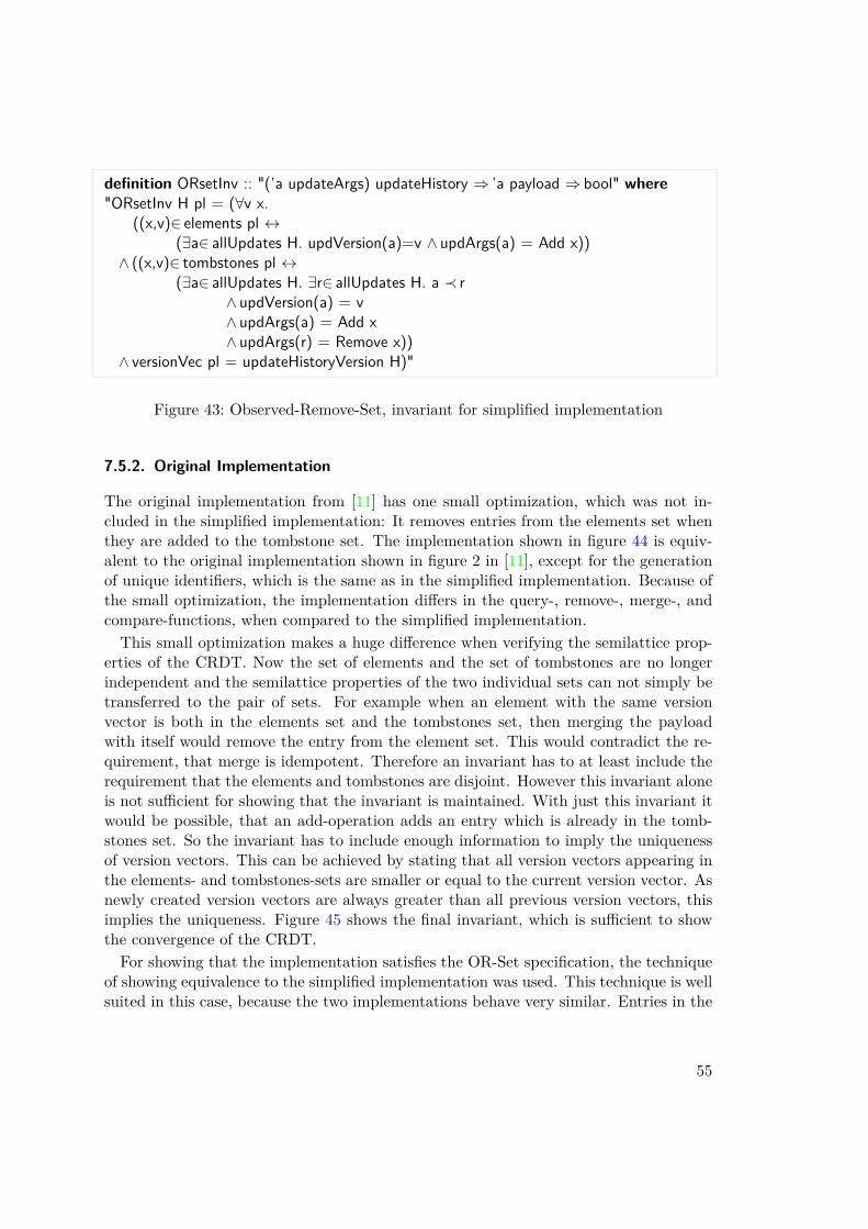
definition ORsetInv :: "(’a updateArgs) updateHistory ⇒ ’a payload ⇒ bool" where"ORsetInv H pl = (∀v x.
((x,v)∈ elements pl ↔(∃a∈ allUpdates H. updVersion(a)=v ∧ updArgs(a) = Add x))
∧ ((x,v)∈ tombstones pl ↔(∃a∈ allUpdates H. ∃r∈ allUpdates H. a ≺ r
∧ updVersion(a) = v∧ updArgs(a) = Add x∧ updArgs(r) = Remove x))
∧ versionVec pl = updateHistoryVersion H)"
Figure 43: Observed-Remove-Set, invariant for simplified implementation
7.5.2. Original Implementation
The original implementation from [11] has one small optimization, which was not in-cluded in the simplified implementation: It removes entries from the elements set whenthey are added to the tombstone set. The implementation shown in figure 44 is equiv-alent to the original implementation shown in figure 2 in [11], except for the generationof unique identifiers, which is the same as in the simplified implementation. Because ofthe small optimization, the implementation differs in the query-, remove-, merge-, andcompare-functions, when compared to the simplified implementation.This small optimization makes a huge difference when verifying the semilattice prop-
erties of the CRDT. Now the set of elements and the set of tombstones are no longerindependent and the semilattice properties of the two individual sets can not simply betransferred to the pair of sets. For example when an element with the same versionvector is both in the elements set and the tombstones set, then merging the payloadwith itself would remove the entry from the element set. This would contradict the re-quirement, that merge is idempotent. Therefore an invariant has to at least include therequirement that the elements and tombstones are disjoint. However this invariant aloneis not sufficient for showing that the invariant is maintained. With just this invariant itwould be possible, that an add-operation adds an entry which is already in the tomb-stones set. So the invariant has to include enough information to imply the uniquenessof version vectors. This can be achieved by stating that all version vectors appearing inthe elements- and tombstones-sets are smaller or equal to the current version vector. Asnewly created version vectors are always greater than all previous version vectors, thisimplies the uniqueness. Figure 45 shows the final invariant, which is sufficient to showthe convergence of the CRDT.For showing that the implementation satisfies the OR-Set specification, the technique
of showing equivalence to the simplified implementation was used. This technique is wellsuited in this case, because the two implementations behave very similar. Entries in the
55

sets have the same version vectors, so no complicated coupling is required. The couplinginvariant is shown in figure 46. Besides the relations between the sets, the coupling alsoincludes the same information about version vectors, as the invariant used for proofingthe convergence of the CRDT. Using this coupling invariant the equivalence of the twoimplementations can be shown in only a few lines of proof code.
56
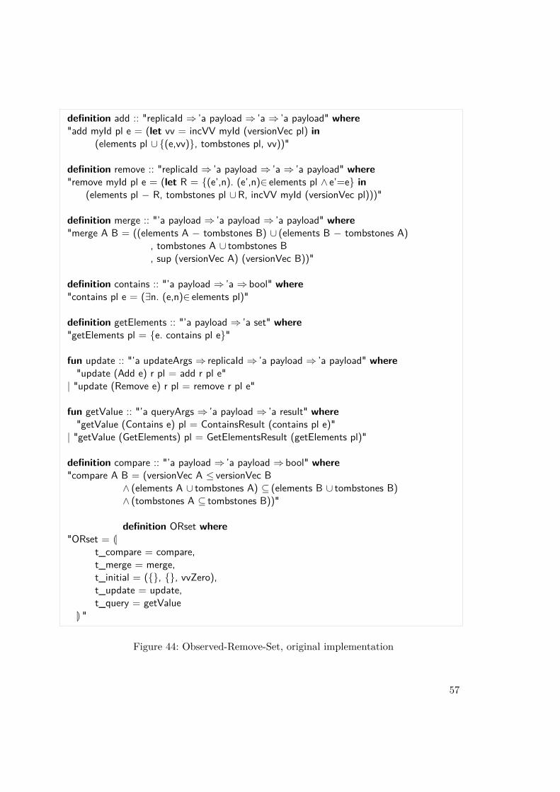
definition add :: "replicaId ⇒ ’a payload ⇒ ’a ⇒ ’a payload" where"add myId pl e = (let vv = incVV myId (versionVec pl) in
(elements pl ∪ {(e,vv)}, tombstones pl, vv))"
definition remove :: "replicaId ⇒ ’a payload ⇒ ’a ⇒ ’a payload" where"remove myId pl e = (let R = {(e’,n). (e’,n)∈ elements pl ∧ e’=e} in
(elements pl − R, tombstones pl ∪R, incVV myId (versionVec pl)))"
definition merge :: "’a payload ⇒ ’a payload ⇒ ’a payload" where"merge A B = ((elements A − tombstones B) ∪ (elements B − tombstones A)
, tombstones A ∪ tombstones B, sup (versionVec A) (versionVec B))"
definition contains :: "’a payload ⇒ ’a ⇒ bool" where"contains pl e = (∃n. (e,n)∈ elements pl)"
definition getElements :: "’a payload ⇒ ’a set" where"getElements pl = {e. contains pl e}"
fun update :: "’a updateArgs ⇒ replicaId ⇒ ’a payload ⇒ ’a payload" where"update (Add e) r pl = add r pl e"
| "update (Remove e) r pl = remove r pl e"
fun getValue :: "’a queryArgs ⇒ ’a payload ⇒ ’a result" where"getValue (Contains e) pl = ContainsResult (contains pl e)"
| "getValue (GetElements) pl = GetElementsResult (getElements pl)"
definition compare :: "’a payload ⇒ ’a payload ⇒ bool" where"compare A B = (versionVec A ≤ versionVec B
∧ (elements A ∪ tombstones A) ⊆ (elements B ∪ tombstones B)∧ (tombstones A ⊆ tombstones B))"
definition ORset where"ORset = L
t_compare = compare,t_merge = merge,t_initial = ({}, {}, vvZero),t_update = update,t_query = getValue
M "
Figure 44: Observed-Remove-Set, original implementation
57
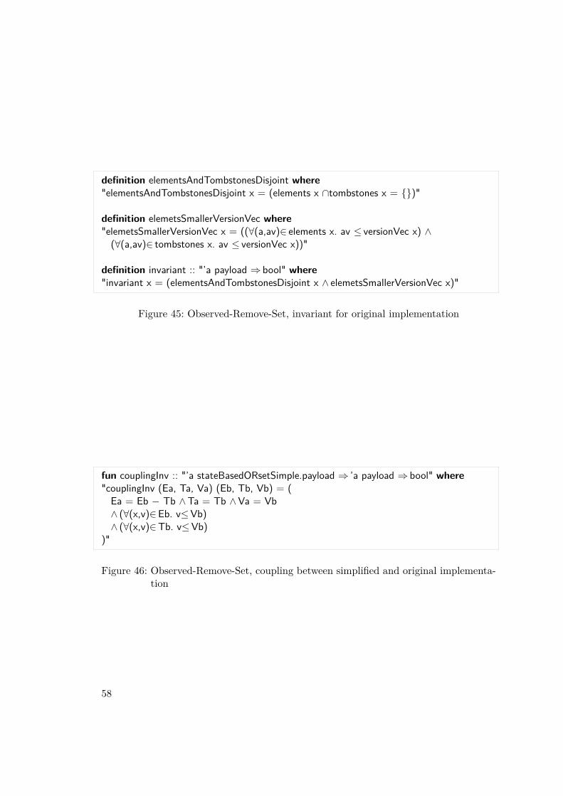
definition elementsAndTombstonesDisjoint where"elementsAndTombstonesDisjoint x = (elements x ∩tombstones x = {})"
definition elemetsSmallerVersionVec where"elemetsSmallerVersionVec x = ((∀(a,av)∈ elements x. av ≤ versionVec x) ∧(∀(a,av)∈ tombstones x. av ≤ versionVec x))"
definition invariant :: "’a payload ⇒ bool" where"invariant x = (elementsAndTombstonesDisjoint x ∧ elemetsSmallerVersionVec x)"
Figure 45: Observed-Remove-Set, invariant for original implementation
fun couplingInv :: "’a stateBasedORsetSimple.payload ⇒ ’a payload ⇒ bool" where"couplingInv (Ea, Ta, Va) (Eb, Tb, Vb) = (Ea = Eb − Tb ∧Ta = Tb ∧Va = Vb∧ (∀(x,v)∈Eb. v≤Vb)∧ (∀(x,v)∈Tb. v≤Vb)
)"
Figure 46: Observed-Remove-Set, coupling between simplified and original implementa-tion
58
7.5.3. Optimized Implementation
The original implementation of the OR-set still stores a lot of redundant information.Every add-operation is represented with an entry in the elements- or tombstones-set. Theoptimized implementation from [1] shows that this is not necessary. The translationof this implementation to Isabelle is shown in figure 47 and figure 48. The Isabelletranslation only covers the state based part of the original optimized OR-Set.The payload of the CRDT consists of two parts. The first part is a version vector,
which counts the number of add-operations on each replica. The second part is a set oftriples (e, c, r) representing add-operations, where e is the added element, r is the replicaon which the element was added, and c is a kind of timestamp. More precisely c is thenumber of add-operations on the same replica, which happened up to and including theadd-operation the triple represents. So for the first add-operation c will be one, for thesecond add-operation it will be two, and so on.The implementation does not need a set of tombstones. It uses the version vector to
decide if an element has been removed from the set. When merging two payloads andboth contain the same triple, then it is certain, that the element has not been removed(set M in the merge function). When neither payload contains a triple for an element itis certain, that the element is not in the set. When one payload contains a triple, whichthe other does not contain, then the version vector is used to check if the add-operationrepresented by that triple has been observed by the other replica. If it has been observed,then the element is removed, otherwise it stays in the set (sets M’ and M’’ in the mergefunction).Another optimization besides the missing tombstones set is the removal of old triples
from the payloads, when there is a triple representing a newer add-operation.
Convergence. The aforementioned optimizations make it difficult to show the semilat-tice properties for this CRDT. The compare function in the original implementation wasnot suited well for showing the semilattice properties and so a different function was used(see figure 48). The problem with the original compare function was, that it assumedsome uniqueness properties, for example that there cannot be two triples (x, c, r) and(y, c, r) with same timestamp and replica but different elements. This is an invariantwhich cannot be described locally. It could be described by describing the relation of thetriples to the update history, but that would make the proofs unnecessary complicated.The new function does not need such an invariant and it corresponds better to the mergefunction, which makes the proofs easier.The invariant used for showing the semilattice properties is shown in figure 49. The
definitions invariant_c_unique and invariant_e_unique describe the fact, that on eachreplica there is at most one timestamp per element and at most one element per times-tamp. The definitions invariant_c_lower_bound and invariant_c_upper_bound state thetimestamps c in the triples are greater than zero and less than the respective componentin the version vector. Showing that this invariant is preserved by updates is very easy,showing that merges preserve the invariant is a bit more difficult, but can also be donewith mainly automatic methods. With this invariant it is possible to show the semilat-
59
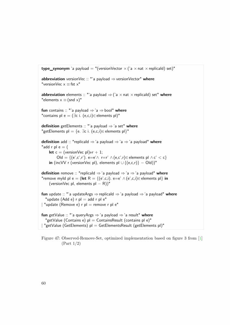
type_synonym ’a payload = "(versionVector × (’a × nat × replicaId) set)"
abbreviation versionVec :: "’a payload ⇒ versionVector" where"versionVec x ≡ fst x"
abbreviation elements :: "’a payload ⇒ (’a × nat × replicaId) set" where"elements x ≡ (snd x)"
fun contains :: "’a payload ⇒ ’a ⇒ bool" where"contains pl e = (∃c i. (e,c,i)∈ elements pl)"
definition getElements :: "’a payload ⇒ ’a set" where"getElements pl = {e. ∃c i. (e,c,i)∈ elements pl}"
definition add :: "replicaId ⇒ ’a payload ⇒ ’a ⇒ ’a payload" where"add r pl e = (
let c = (versionVec pl)»r + 1;Old = {(e’,c’,r’). e=e’∧ r=r’ ∧ (e,c’,r)∈ elements pl ∧ c’ < c}
in (incVV r (versionVec pl), elements pl ∪ {(e,c,r)} − Old))"
definition remove :: "replicaId ⇒ ’a payload ⇒ ’a ⇒ ’a payload" where"remove myId pl e = (let R = {(e’,c,i). e=e’ ∧ (e’,c,i)∈ elements pl} in
(versionVec pl, elements pl − R))"
fun update :: "’a updateArgs ⇒ replicaId ⇒ ’a payload ⇒ ’a payload" where"update (Add e) r pl = add r pl e"
| "update (Remove e) r pl = remove r pl e"
fun getValue :: "’a queryArgs ⇒ ’a payload ⇒ ’a result" where"getValue (Contains e) pl = ContainsResult (contains pl e)"
| "getValue (GetElements) pl = GetElementsResult (getElements pl)"
Figure 47: Observed-Remove-Set, optimized implementation based on figure 3 from [1](Part 1/2)
60
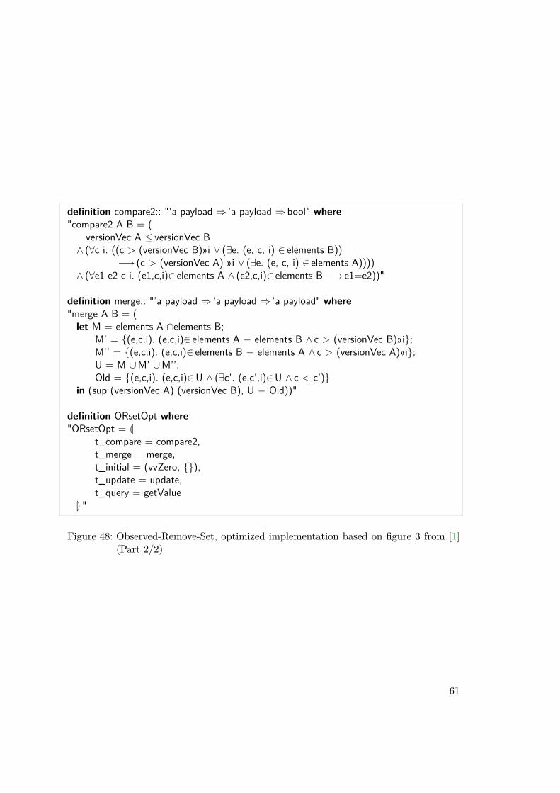
definition compare2:: "’a payload ⇒ ’a payload ⇒ bool" where"compare2 A B = (
versionVec A ≤ versionVec B∧ (∀c i. ((c > (versionVec B)»i ∨ (∃e. (e, c, i) ∈ elements B))
−→ (c > (versionVec A) »i ∨ (∃e. (e, c, i) ∈ elements A))))∧ (∀e1 e2 c i. (e1,c,i)∈ elements A ∧ (e2,c,i)∈ elements B −→ e1=e2))"
definition merge:: "’a payload ⇒ ’a payload ⇒ ’a payload" where"merge A B = (let M = elements A ∩elements B;
M’ = {(e,c,i). (e,c,i)∈ elements A − elements B ∧ c > (versionVec B)»i};M’’ = {(e,c,i). (e,c,i)∈ elements B − elements A ∧ c > (versionVec A)»i};U = M ∪M’ ∪M’’;Old = {(e,c,i). (e,c,i)∈U ∧ (∃c’. (e,c’,i)∈U ∧ c < c’)}
in (sup (versionVec A) (versionVec B), U − Old))"
definition ORsetOpt where"ORsetOpt = L
t_compare = compare2,t_merge = merge,t_initial = (vvZero, {}),t_update = update,t_query = getValue
M "
Figure 48: Observed-Remove-Set, optimized implementation based on figure 3 from [1](Part 2/2)
61
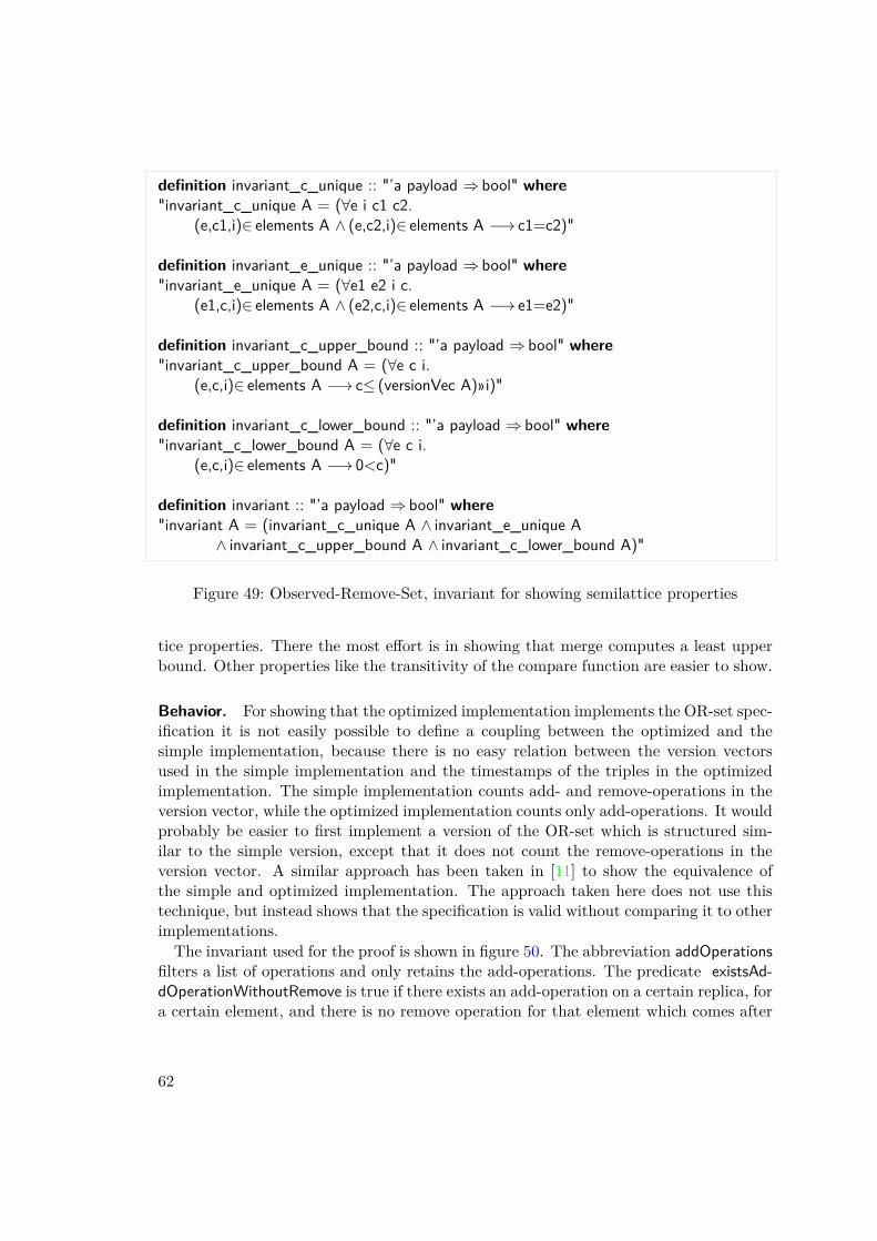
definition invariant_c_unique :: "’a payload ⇒ bool" where"invariant_c_unique A = (∀e i c1 c2.
(e,c1,i)∈ elements A ∧ (e,c2,i)∈ elements A −→ c1=c2)"
definition invariant_e_unique :: "’a payload ⇒ bool" where"invariant_e_unique A = (∀e1 e2 i c.
(e1,c,i)∈ elements A ∧ (e2,c,i)∈ elements A −→ e1=e2)"
definition invariant_c_upper_bound :: "’a payload ⇒ bool" where"invariant_c_upper_bound A = (∀e c i.
(e,c,i)∈ elements A −→ c≤ (versionVec A)»i)"
definition invariant_c_lower_bound :: "’a payload ⇒ bool" where"invariant_c_lower_bound A = (∀e c i.
(e,c,i)∈ elements A −→ 0<c)"
definition invariant :: "’a payload ⇒ bool" where"invariant A = (invariant_c_unique A ∧ invariant_e_unique A
∧ invariant_c_upper_bound A ∧ invariant_c_lower_bound A)"
Figure 49: Observed-Remove-Set, invariant for showing semilattice properties
tice properties. There the most effort is in showing that merge computes a least upperbound. Other properties like the transitivity of the compare function are easier to show.
Behavior. For showing that the optimized implementation implements the OR-set spec-ification it is not easily possible to define a coupling between the optimized and thesimple implementation, because there is no easy relation between the version vectorsused in the simple implementation and the timestamps of the triples in the optimizedimplementation. The simple implementation counts add- and remove-operations in theversion vector, while the optimized implementation counts only add-operations. It wouldprobably be easier to first implement a version of the OR-set which is structured sim-ilar to the simple version, except that it does not count the remove-operations in theversion vector. A similar approach has been taken in [11] to show the equivalence ofthe simple and optimized implementation. The approach taken here does not use thistechnique, but instead shows that the specification is valid without comparing it to otherimplementations.The invariant used for the proof is shown in figure 50. The abbreviation addOperations
filters a list of operations and only retains the add-operations. The predicate existsAd-dOperationWithoutRemove is true if there exists an add-operation on a certain replica, fora certain element, and there is no remove operation for that element which comes after
62
the add-operation. The invariant consists of three parts A, B, and C. Part A describesthe contents of the version vector. Each component of the version vector is equal tothe number of add-operations on the respective replica. Part B describes when a tripleis in the set of elements. When there is an add operation for x on replica r without alater remove operation for x, then there exists a c so that the triple (x, c, r) is in the set.Otherwise no such triple exists in the set. Part C describes what it means for a triple(x, c, r) to be in the set of elements. This part contains several properties. First, it givesthe same bounds to the timestamp c, as were used in the verification of the semilatticeproperties. Then, it states that the c-th element in the list of add-operations adds theelement x to the set, and as last point part C states, that after that add-operation, therecomes no other add-operation, which adds the same element x on the same replica r.Part B of the invariant is enough to show that the invariant implies the specification
and it can easily be seen, that this part implies the specification. The other parts areimportant for proving that the invariant is maintained. In this part of the proof the maindifficulties are in the case for the merge operation and part B of the invariant, as thereare many cases to be considered. There are a few more complex cases, which mostly area result of the rather complicated relation between timestamps c and the position of theadd-operations in the filtered list.
63
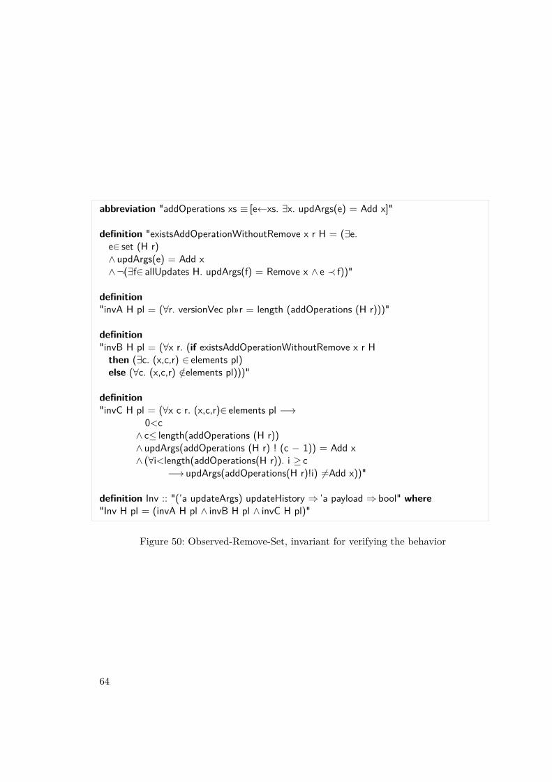
abbreviation "addOperations xs ≡ [e←xs. ∃x. updArgs(e) = Add x]"
definition "existsAddOperationWithoutRemove x r H = (∃e.e∈ set (H r)∧ updArgs(e) = Add x∧¬(∃f∈ allUpdates H. updArgs(f) = Remove x ∧ e ≺ f))"
definition"invA H pl = (∀r. versionVec pl»r = length (addOperations (H r)))"
definition"invB H pl = (∀x r. (if existsAddOperationWithoutRemove x r Hthen (∃c. (x,c,r) ∈ elements pl)else (∀c. (x,c,r) /∈elements pl)))"
definition"invC H pl = (∀x c r. (x,c,r)∈ elements pl −→
0<c∧ c≤ length(addOperations (H r))∧ updArgs(addOperations (H r) ! (c − 1)) = Add x∧ (∀i<length(addOperations(H r)). i ≥ c
−→ updArgs(addOperations(H r)!i) 6=Add x))"
definition Inv :: "(’a updateArgs) updateHistory ⇒ ’a payload ⇒ bool" where"Inv H pl = (invA H pl ∧ invB H pl ∧ invC H pl)"
Figure 50: Observed-Remove-Set, invariant for verifying the behavior
64
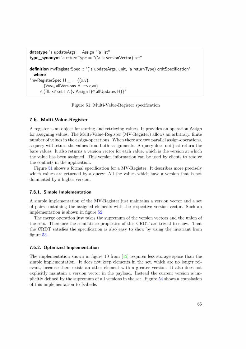
datatype ’a updateArgs = Assign "’a list"type_synonym ’a returnType = "(’a × versionVector) set"
definition mvRegisterSpec :: "(’a updateArgs, unit, ’a returnType) crdtSpecification"where
"mvRegisterSpec H _ = {(x,v).(∀vv∈ allVersions H. ¬v<vv)∧ (∃l. x∈ set l ∧ (v,Assign l)∈ allUpdates H)}"
Figure 51: Multi-Value-Register specification
7.6. Multi-Value-Register
A register is an object for storing and retrieving values. It provides an operation Assignfor assigning values. The Multi-Value-Register (MV-Register) allows an arbitrary, finitenumber of values in the assign-operations. When there are two parallel assign-operations,a query will return the values from both assignments. A query does not just return thebare values. It also returns a version vector for each value, which is the version at whichthe value has been assigned. This version information can be used by clients to resolvethe conflicts in the application.Figure 51 shows a formal specification for a MV-Register. It describes more precisely
which values are returned by a query: All the values which have a version that is notdominated by a higher version.
7.6.1. Simple Implementation
A simple implementation of the MV-Register just maintains a version vector and a setof pairs containing the assigned elements with the respective version vector. Such animplementation is shown in figure 52.The merge operation just takes the supremum of the version vectors and the union of
the sets. Therefore the semilattice properties of this CRDT are trivial to show. Thatthe CRDT satisfies the specification is also easy to show by using the invariant fromfigure 53.
7.6.2. Optimized Implementation
The implementation shown in figure 10 from [12] requires less storage space than thesimple implementation. It does not keep elements in the set, which are no longer rel-evant, because there exists an other element with a greater version. It also does notexplicitly maintain a version vector in the payload. Instead the current version is im-plicitly defined by the supremum of all versions in the set. Figure 54 shows a translationof this implementation to Isabelle.
65
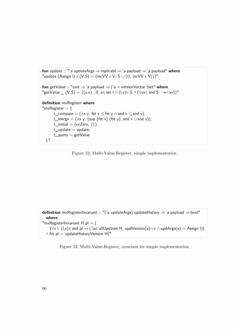
fun update :: "’a updateArgs ⇒ replicaId ⇒ ’a payload ⇒ ’a payload" where"update (Assign l) r (V,S) = (incVV r V, S ∪ {(l, incVV r V)})"
fun getValue :: "unit ⇒ ’a payload ⇒ (’a × versionVector )set" where"getValue _ (V,S) = {(x,v). ∃l. x∈ set l ∧ (l,v)∈S ∧ (∀vv∈ snd‘S. ¬v<vv)}"
definition mvRegister where"mvRegister = L
t_compare = (λx y. fst x ≤ fst y ∧ snd x ⊆ snd y),t_merge = (λx y. (sup (fst x) (fst y), snd x ∪ snd y)),t_initial = (vvZero, {}),t_update = update,t_query = getValue
M "
Figure 52: Multi-Value-Register, simple implementation
definition mvRegisterInvariant :: "(’a updateArgs) updateHistory ⇒ ’a payload ⇒ bool"where
"mvRegisterInvariant H pl = ((∀v l. (l,v)∈ snd pl ↔ (∃a∈ allUpdates H. updVersion(a)=v ∧ updArgs(a) = Assign l))∧ fst pl = updateHistoryVersion H)"
Figure 53: Multi-Value-Register, invariant for simple implementation
66
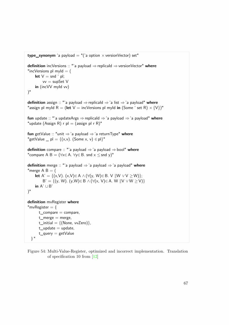
type_synonym ’a payload = "(’a option × versionVector) set"
definition incVersions :: "’a payload ⇒ replicaId ⇒ versionVector" where"incVersions pl myId = (
let V = snd ‘ pl;vv = supSet V
in (incVV myId vv))"
definition assign :: "’a payload ⇒ replicaId ⇒ ’a list ⇒ ’a payload" where"assign pl myId R = (let V = incVersions pl myId in (Some ‘ set R) × {V})"
fun update :: "’a updateArgs ⇒ replicaId ⇒ ’a payload ⇒ ’a payload" where"update (Assign R) r pl = (assign pl r R)"
fun getValue :: "unit ⇒ ’a payload ⇒ ’a returnType" where"getValue _ pl = {(x,v). (Some x, v) ∈ pl}"
definition compare :: "’a payload ⇒ ’a payload ⇒ bool" where"compare A B = (∀x∈A. ∀y∈B. snd x ≤ snd y)"
definition merge :: "’a payload ⇒ ’a payload ⇒ ’a payload" where"merge A B = (
let A’ = {(x,V). (x,V)∈A ∧ (∀(y, W)∈B. V ‖W ∨V ≥W)};B’ = {(y, W). (y,W)∈B ∧ (∀(x, V)∈A. W ‖V ∨W ≥V)}
in A’ ∪B’)"
definition mvRegister where"mvRegister = L
t_compare = compare,t_merge = merge,t_initial = {(None, vvZero)},t_update = update,t_query = getValue
M "
Figure 54: Multi-Value-Register, optimized and incorrect implementation. Translationof specification 10 from [12]
67
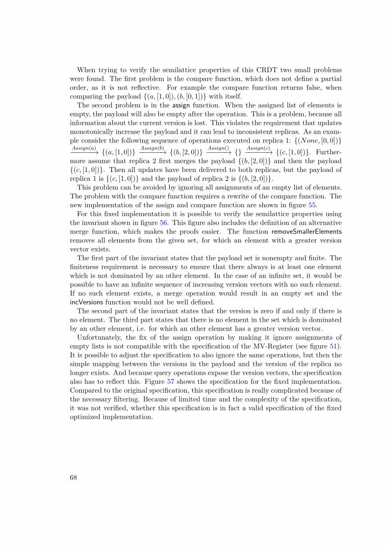
When trying to verify the semilattice properties of this CRDT two small problemswere found. The first problem is the compare function, which does not define a partialorder, as it is not reflective. For example the compare function returns false, whencomparing the payload {(a, [1, 0]), (b, [0, 1])} with itself.The second problem is in the assign function. When the assigned list of elements is
empty, the payload will also be empty after the operation. This is a problem, because allinformation about the current version is lost. This violates the requirement that updatesmonotonically increase the payload and it can lead to inconsistent replicas. As an exam-ple consider the following sequence of operations executed on replica 1: {(None, [0, 0])}Assign(a)−−−−−−→ {(a, [1, 0])} Assign(b)−−−−−−→ {(b, [2, 0])} Assign()−−−−−→ {} Assign(c)−−−−−−→ {(c, [1, 0])}. Further-more assume that replica 2 first merges the payload {(b, [2, 0])} and then the payload{(c, [1, 0])}. Then all updates have been delivered to both replicas, but the payload ofreplica 1 is {(c, [1, 0])} and the payload of replica 2 is {(b, [2, 0])}.This problem can be avoided by ignoring all assignments of an empty list of elements.
The problem with the compare function requires a rewrite of the compare function. Thenew implementation of the assign and compare function are shown in figure 55.For this fixed implementation it is possible to verify the semilattice properties using
the invariant shown in figure 56. This figure also includes the definition of an alternativemerge function, which makes the proofs easier. The function removeSmallerElementsremoves all elements from the given set, for which an element with a greater versionvector exists.The first part of the invariant states that the payload set is nonempty and finite. The
finiteness requirement is necessary to ensure that there always is at least one elementwhich is not dominated by an other element. In the case of an infinite set, it would bepossible to have an infinite sequence of increasing version vectors with no such element.If no such element exists, a merge operation would result in an empty set and theincVersions function would not be well defined.The second part of the invariant states that the version is zero if and only if there is
no element. The third part states that there is no element in the set which is dominatedby an other element, i.e. for which an other element has a greater version vector.Unfortunately, the fix of the assign operation by making it ignore assignments of
empty lists is not compatible with the specification of the MV-Register (see figure 51).It is possible to adjust the specification to also ignore the same operations, but then thesimple mapping between the versions in the payload and the version of the replica nolonger exists. And because query operations expose the version vectors, the specificationalso has to reflect this. Figure 57 shows the specification for the fixed implementation.Compared to the original specification, this specification is really complicated because ofthe necessary filtering. Because of limited time and the complexity of the specification,it was not verified, whether this specification is in fact a valid specification of the fixedoptimized implementation.
68
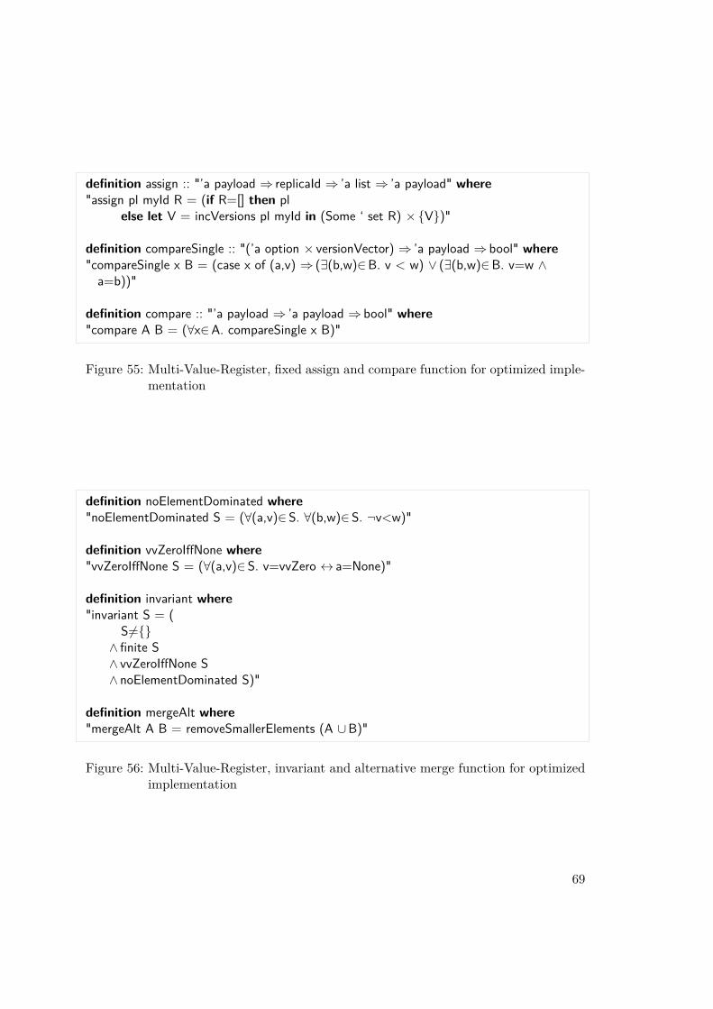
definition assign :: "’a payload ⇒ replicaId ⇒ ’a list ⇒ ’a payload" where"assign pl myId R = (if R=[] then pl
else let V = incVersions pl myId in (Some ‘ set R) × {V})"
definition compareSingle :: "(’a option × versionVector) ⇒ ’a payload ⇒ bool" where"compareSingle x B = (case x of (a,v) ⇒ (∃(b,w)∈B. v < w) ∨ (∃(b,w)∈B. v=w ∧a=b))"
definition compare :: "’a payload ⇒ ’a payload ⇒ bool" where"compare A B = (∀x∈A. compareSingle x B)"
Figure 55: Multi-Value-Register, fixed assign and compare function for optimized imple-mentation
definition noElementDominated where"noElementDominated S = (∀(a,v)∈S. ∀(b,w)∈S. ¬v<w)"
definition vvZeroIffNone where"vvZeroIffNone S = (∀(a,v)∈S. v=vvZero ↔ a=None)"
definition invariant where"invariant S = (
S 6={}∧ finite S∧ vvZeroIffNone S∧ noElementDominated S)"
definition mergeAlt where"mergeAlt A B = removeSmallerElements (A ∪B)"
Figure 56: Multi-Value-Register, invariant and alternative merge function for optimizedimplementation
69
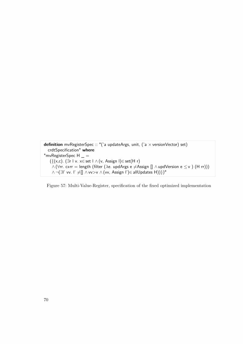
definition mvRegisterSpec :: "(’a updateArgs, unit, (’a × versionVector) set)crdtSpecification" where
"mvRegisterSpec H _ =({(x,c). (∃r l v. x∈ set l ∧ (v, Assign l)∈ set(H r)∧ (∀rr. c»rr = length (filter (λe. updArgs e 6=Assign [] ∧ updVersion e ≤ v ) (H rr)))∧¬(∃l’ vv. l’ 6=[] ∧ vv>v ∧ (vv, Assign l’)∈ allUpdates H))})"
Figure 57: Multi-Value-Register, specification of the fixed optimized implementation
70
8. Related workThere exists work by Christopher Meiklejohn, which uses the interactive theorem proverCoq for verifying semilattice properties of CRDTs[7, 8, 9]. The behavioral propertiesof CRDTs are not considered. Verified CRDTs are the increase-only-counter and thePN-counter. In contrast to this thesis the verification is not based on a formal systemmodel. Instead the semilattice properties are verified standing alone, but this is nota problem, because it is known from the literature[12], that the semilattice propertieswith monotonic updates are a sufficient condition for convergence. However the verifiedsemilattice properties are slightly different than the properties used in this thesis. Insteadof showing that merge computes a least upper bound, it is only shown that it computesan upper bound and that the operation is commutative, idempotent and associative.The last three properties are equivalent to the computation of a least upper bound,when the compare function satisfies the equation compare x y ↔ (merge x y = y), butthis equation is not verified. It would be interesting to check if the verified conditionsare sufficient for convergence, as well.Another work including verification of CRDTs is Replicated Data Types: Specification,
Verification, Optimality[3]. This paper follows a similar approach of basing the theoryon a system model and it follows a very similar approach in specifying and verifying thebehavior of CRDTs. In the paper no use of a tool for the verification is mentioned, so itcan be assumed that the proofs are not machine checked.The basic system model is more flexible than the system model used in this thesis.
The model uses explicit send- and receive- actions, where the send actions also canhave side-effects on the payload. This feature allows to also emulate operation-basedCRDTs in the model, by caching the effect of operations locally and then send themin a batch of operations. The system also has a more flexible notation of visibility,than the visibility which was defined by version vectors in this thesis and the systemsupports timestamps, which allows having data types like the Last-Writer-Wins-Register.While the system is more flexible, only state-based CRDTs are verified, and except fortimestamps the flexibility of the system is not used in the state-based implementations.For the verification the flexible parameters of the system are instantiated so that theresult is a system, which is very close to the system used in this thesis. In the paper thebehavior of the Increment-Only-Counter, a Last-Writer-Wins-Register and a optimizedOR-Set are verified. The OR-Set has a slightly different structure than the OR-Setverified in this thesis, but is basically equivalent.
71

9. Conclusion and future workThe case studies have shown, that it is feasible to verify CRDTs with Isabelle/HOL.The problem found in the MV-register during verification, shows that it is easy to misssome corner case when designing a CRDT. The verified CRDTs were given in pseudo-language and then translated to Isabelle, which is a very high level language. Realimplementations of the same CRDTs will probably be more complex, and thus thechance of introducing bugs might be even higher. But also the amount of work requiredfor verifying a real implementation is higher. The framework presented in this thesis isnot directly applicable to real implementations. Several approaches are possible to closethe gap between the verified Isabelle code and a real implementation:
1. Isabelle can generate code for the languages SML, OCaml, Haskell and Scala fromthe Isabelle code. An advantage of using this approach would be that there is areal end-to-end verification from the abstract system model to the executable code.So there would only be the system model, the specification of the specific CRDT,and the Isabelle tool, which would have to be trusted, as the rest is verified to becorrect. A disadvantage is, that the generated code is not very readable and notvery efficient. Also, the generated code does not use the default data types of thelanguage, so probably some wrapper code would be necessary to conform with thenecessary interfaces.
2. It would be possible to describe CRDTs in a domain specific language and generateIsabelle code and executable code from this description. This approach would bemore flexible in the generation of the executable code, so that the code couldbe more readable, efficient and be compliant to the necessary interfaces. Theadvantages come at the cost of more possible points of failures. With this approachone additionally has to trust the code generator for the domain specific language.
3. The executable code could be written manually and then it could be verified thatthe executable code is equivalent to the more abstract Isabelle code. This can bedone separately for each function. As there is no concurrency inside a function(each update and merge is executed on a single replica) this equivalence can beshown using techniques and tools for sequential programs. This approach is veryflexible in what can be done in the implementation of the executable code, but ithas more possible points of failure than the first two approaches.
There are some other challenges in real system which could be addressed in futurework. One problem is the space complexity of payloads. Because of the requirementfor monotonically increasing updates the required space for storing the payload is alsoincreasing with time. Optimized implementations like the optimized OR-Set can reducethe space complexity, but there are limits for the possible optimizations [3]. Furthermore,in real systems replicas can be dynamically added to and removed from the system,and data which references removed nodes should also be garbage-collected. Thereforelong-running systems will probably need a form of garbage-collection. With the system
73
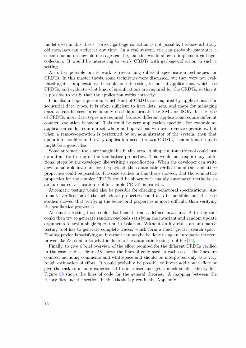
model used in this thesis, correct garbage collection is not possible, because arbitraryold messages can arrive at any time. In a real system, one can probably guarantee acertain bound on how old messages can be, and this would allow to implement garbage-collection. It would be interesting to verify CRDTs with garbage-collection in such asetting.An other possible future work is researching different specification techniques for
CRDTs. In this master thesis, some techniques were discussed, but they were not eval-uated against applications. It would be interesting to look at applications, which useCRDTs, and evaluate what kind of specifications are required for the CRDTs, so that itis possible to verify that the application works correctly.It is also an open question, which kind of CRDTs are required by applications. For
sequential data types, it is often sufficient to have lists, sets, and maps for managingdata, as can be seen in commonly used data formats like XML or JSON. In the caseof CRDTs, more data types are required, because different applications require differentconflict resolution behavior. This could be very application specific. For example anapplication could require a set where add-operations win over remove-operations, butwhen a remove-operation is performed by an administrator of the system, then thatoperation should win. If every application needs its own CRDTs, then automatic toolsmight be a good idea.Some automatic tools are imaginable in this area. A simple automatic tool could just
do automatic testing of the semilattice properties. This would not require any addi-tional steps by the developer like writing a specification. When the developer can writedown a suitable invariant for the payload, then automatic verification of the semilatticeproperties could be possible. The case studies in this thesis showed, that the semilatticeproperties for the simpler CRDTs could be shown with mainly automated methods, soan automated verification tool for simple CRDTs is realistic.Automatic testing would also be possible for checking behavioral specifications. Au-
tomatic verification of the behavioral properties could also be possible, but the casestudies showed that verifying the behavioral properties is more difficult, than verifyingthe semilattice properties.Automatic testing tools could also benefit from a defined invariant. A testing tool
could then try to generate random payloads satisfying the invariant and random updatearguments to test a single operation in isolation. Without an invariant, an automatedtesting tool has to generate complete traces, which form a much greater search space.Finding payloads satisfying an invariant can maybe be done using an automatic theoremprover like Z3, similar to what is done in the automatic testing tool Pex[13].Finally, to give a brief overview of the effort required for the different CRDTs verified
in the case studies, figure 58 shows the lines of code used in each case. The lines arecounted including comments and whitespace and should be interpreted only as a veryrough estimation of effort. It would probably be possible to invest additional effort orgive the task to a more experienced Isabelle user and get a much smaller theory file.Figure 59 shows the lines of code for the general theories. A mapping between thetheory files and the sections in this thesis is given in the Appendix.
74
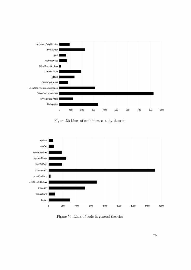
Figure 58: Lines of code in case study theories
Figure 59: Lines of code in general theories
75

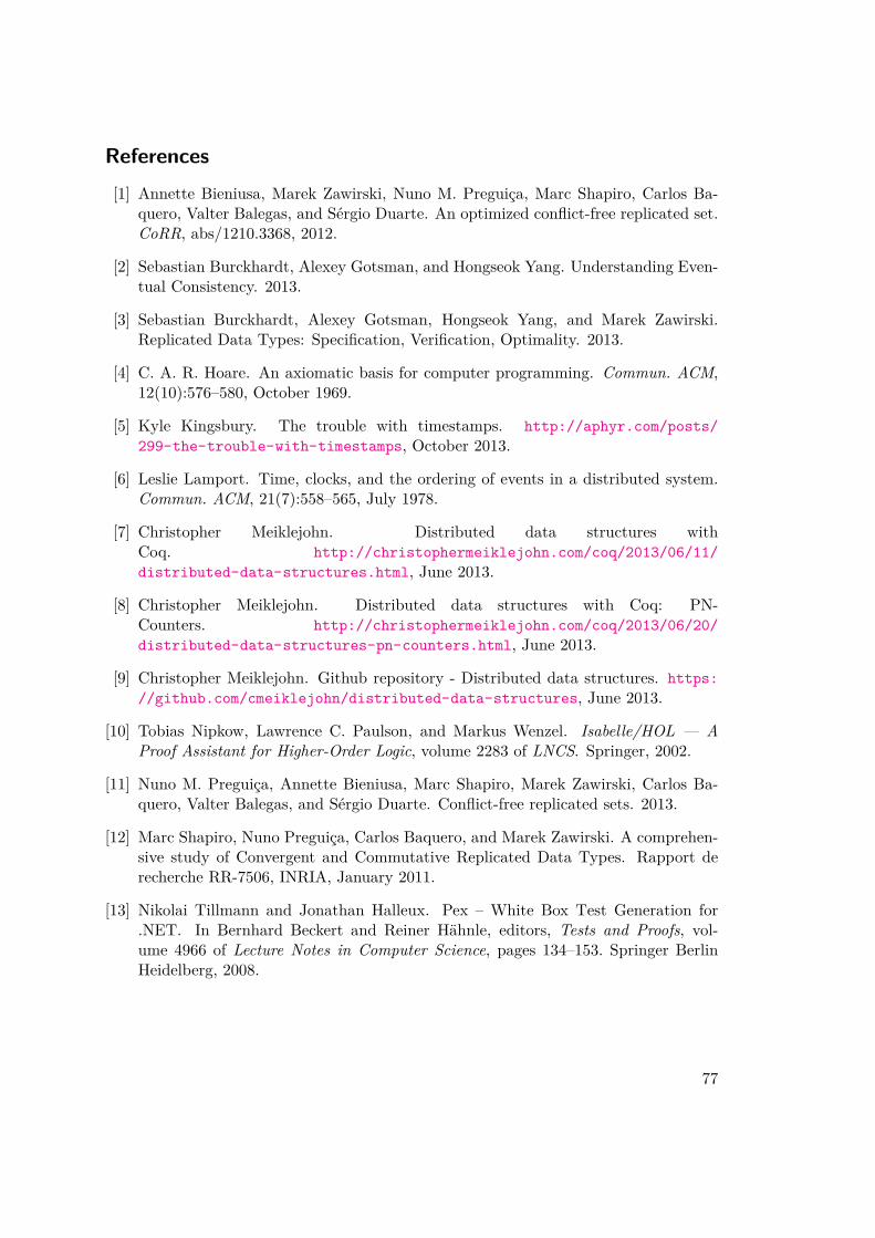
References[1] Annette Bieniusa, Marek Zawirski, Nuno M. Preguiça, Marc Shapiro, Carlos Ba-
quero, Valter Balegas, and Sérgio Duarte. An optimized conflict-free replicated set.CoRR, abs/1210.3368, 2012.
[2] Sebastian Burckhardt, Alexey Gotsman, and Hongseok Yang. Understanding Even-tual Consistency. 2013.
[3] Sebastian Burckhardt, Alexey Gotsman, Hongseok Yang, and Marek Zawirski.Replicated Data Types: Specification, Verification, Optimality. 2013.
[4] C. A. R. Hoare. An axiomatic basis for computer programming. Commun. ACM,12(10):576–580, October 1969.
[5] Kyle Kingsbury. The trouble with timestamps. http://aphyr.com/posts/299-the-trouble-with-timestamps, October 2013.
[6] Leslie Lamport. Time, clocks, and the ordering of events in a distributed system.Commun. ACM, 21(7):558–565, July 1978.
[7] Christopher Meiklejohn. Distributed data structures withCoq. http://christophermeiklejohn.com/coq/2013/06/11/distributed-data-structures.html, June 2013.
[8] Christopher Meiklejohn. Distributed data structures with Coq: PN-Counters. http://christophermeiklejohn.com/coq/2013/06/20/distributed-data-structures-pn-counters.html, June 2013.
[9] Christopher Meiklejohn. Github repository - Distributed data structures. https://github.com/cmeiklejohn/distributed-data-structures, June 2013.
[10] Tobias Nipkow, Lawrence C. Paulson, and Markus Wenzel. Isabelle/HOL — AProof Assistant for Higher-Order Logic, volume 2283 of LNCS. Springer, 2002.
[11] Nuno M. Preguiça, Annette Bieniusa, Marc Shapiro, Marek Zawirski, Carlos Ba-quero, Valter Balegas, and Sérgio Duarte. Conflict-free replicated sets. 2013.
[12] Marc Shapiro, Nuno Preguiça, Carlos Baquero, and Marek Zawirski. A comprehen-sive study of Convergent and Commutative Replicated Data Types. Rapport derecherche RR-7506, INRIA, January 2011.
[13] Nikolai Tillmann and Jonathan Halleux. Pex – White Box Test Generation for.NET. In Bernhard Beckert and Reiner Hähnle, editors, Tests and Proofs, vol-ume 4966 of Lecture Notes in Computer Science, pages 134–153. Springer BerlinHeidelberg, 2008.
77

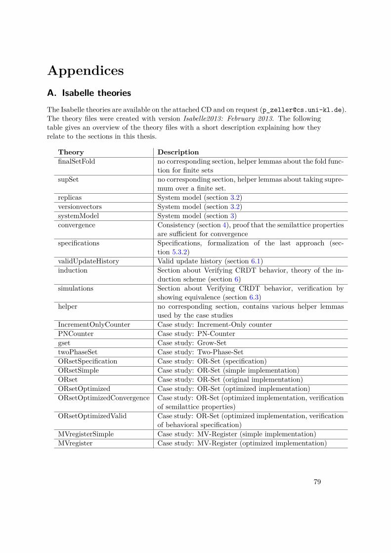
AppendicesA. Isabelle theoriesThe Isabelle theories are available on the attached CD and on request ([email protected]).The theory files were created with version Isabelle2013: February 2013. The followingtable gives an overview of the theory files with a short description explaining how theyrelate to the sections in this thesis.
Theory DescriptionfinalSetFold no corresponding section, helper lemmas about the fold func-
tion for finite setssupSet no corresponding section, helper lemmas about taking supre-
mum over a finite set.replicas System model (section 3.2)versionvectors System model (section 3.2)systemModel System model (section 3)convergence Consistency (section 4), proof that the semilattice properties
are sufficient for convergencespecifications Specifications, formalization of the last approach (sec-
tion 5.3.2)validUpdateHistory Valid update history (section 6.1)induction Section about Verifying CRDT behavior, theory of the in-
duction scheme (section 6)simulations Section about Verifying CRDT behavior, verification by
showing equivalence (section 6.3)helper no corresponding section, contains various helper lemmas
used by the case studiesIncrementOnlyCounter Case study: Increment-Only counterPNCounter Case study: PN-Countergset Case study: Grow-SettwoPhaseSet Case study: Two-Phase-SetORsetSpecification Case study: OR-Set (specification)ORsetSimple Case study: OR-Set (simple implementation)ORset Case study: OR-Set (original implementation)ORsetOptimized Case study: OR-Set (optimized implementation)ORsetOptimizedConvergence Case study: OR-Set (optimized implementation, verification
of semilattice properties)ORsetOptimizedValid Case study: OR-Set (optimized implementation, verification
of behavioral specification)MVregisterSimple Case study: MV-Register (simple implementation)MVregister Case study: MV-Register (optimized implementation)
79