Spectral Empirical Orthogonal Function Analysis of Weather andClimate Data

OLIVER T. SCHMIDT

University of California San Diego, La Jolla, California

GIANMARCO MENGALDO

California Institute of Technology, Pasadena, California

GIANPAOLO BALSAMO AND NILS P. WEDI

European Centre for Medium-Range Weather Forecasts, Reading, United Kingdom

(Manuscript received 26 September 2018, in final form 26 April 2019)

ABSTRACT

We apply spectral empirical orthogonal function (SEOF) analysis to educe climate patterns as dominant

spatiotemporal modes of variability from reanalysis data. SEOF is a frequency-domain variant of standard

empirical orthogonal function (EOF) analysis, and computes modes that represent the statistically most

relevant and persistent patterns from an eigendecomposition of the estimated cross-spectral density matrix

(CSD). The spectral estimation step distinguishes the approach from other frequency-domain EOF

methods based on a single realization of the Fourier transform, and results in a number of desirable

mathematical properties: at each frequency, SEOF yields a set of orthogonal modes that are optimally

ranked in terms of variance in the L2 sense, and that are coherent in both space and time by construction.

We discuss the differences between SEOF and other competing approaches, as well as its relation to dy-

namical modes of stochastically forced, nonnormal linear dynamical systems. The method is applied to

ERA-Interim and ERA-20C reanalysis data, demonstrating its ability to identify a number of well-known

spatiotemporal coherent meteorological patterns and teleconnections, including the Madden–Julian os-

cillation (MJO), the quasi-biennial oscillation (QBO), and the El Niño–Southern Oscillation (ENSO)

(i.e., a range of phenomena reoccurring with average periods ranging from months to many years). In

addition to two-dimensional univariate analyses of surface data, we give examples of multivariate and

three-dimensional meteorological patterns that illustrate how this technique can systematically identify

coherent structures from different sets of data. The MATLAB code used to compute the results presented

in this study, including the download scripts for the reanalysis data, is freely available online.

1. Introduction

Coherent spatiotemporal structures are pervasive in

nature and their systematic identification can help char-

acterize the behavior of complex systems and facilitate

their modeling. Earth’s atmosphere and its complex

coupling to other Earth system components such as

ocean, sea ice, and land surfaces, exhibits many of these

structures. Several statistically persistent patterns asso-

ciated with the intrinsic variability of the Earth system

exist, and these usually play a critical role in extended-

range and seasonal forecasting of both regional and

global-scale weather phenomena (see, e.g., Palmer and

Anderson 1994; Wu et al. 2009; Bierkens and Van Beek

2009). The representation and understanding of these

coherent structures through a reduced and compact set

of predictors can enhance the predictability of the Earth

system and ultimately increase the accuracy of seasonal

forecasting. This idea is certainly not new and dates back

to Lorenz (1956), who highlighted the links between the

so-called dynamical and statistical weather forecasting.

The former is based on a set of equations describing the

physics of the atmosphere (more generally of the Earth

system), while the latter uses statistical tools to infer the

state of the Earth system at a future time, without any

knowledge of the physical mechanisms underlying theCorresponding author: Oliver T. Schmidt, oschmidt@ucsd.edu

system itself. Due to the impact of initial and boundary

conditions that are determined with increasing accuracy,

the dynamical approach is preferred, as the behavior of

the Earth system is efficiently modeled via a set of gov-

erning equations that produce accurate weather forecasts

especially in the short (up to three days ahead) and

medium range (up to two weeks ahead). However, for

extended-range (one month ahead) and seasonal (up to

one year ahead) weather prediction, anomalies in the

turbulent atmospheric floware relevant, and their efficient

characterization in terms of spatiotemporal modes of

variability, associated with global teleconnections as well

as regional phenomena of the Earth system, are of para-

mount importance to enhance long-range predictability.

Themost commonmethod adopted within the weather

and climate community to identify coherent structures is

called empirical orthogonal function (EOF) analysis

(Obukhov 1947; Lorenz 1956; Kutzbach 1967)—see also

Hannachi et al. (2007) for a comprehensive review of

this technique and related extensions, and Navarra and

Simoncini (2010) for a practical guide of traditional EOF

methods applied to climate data. Standard EOF analysis,

also known as proper orthogonal decomposition (POD),

principle component analysis (PCA), Karhunen–Loèvetransform (KLT), or Hotelling transform, is a modal de-

composition technique that extracts coherent structures,

or patterns, in the form of modes of variability from data.

These modes are computed as the eigenvectors of the

(spatially weighted) anomaly covariance matrix. The

corresponding eigenvalues measure the variance and

optimally rank the modes. The Karhunen–Loève pro-

cedure was first derived by Schmidt (1907) and the reader

is referred to Sirovich and Everson (1992) for a com-

prehensive historical review.

In the past few decades, traditional andmore advanced

variants of this technique have been used to study the

modes of variability and the predictability of the Earth

system. For example, Davis (1976) explores sea level

pressure and sea surface temperature anomalies using

EOF. Similarly, Weare et al. (1976) and Weare and

Newell (1977) use EOF to investigate sea surface tem-

perature of both the Atlantic and Pacific Oceans and

Barnett (1978) analyzes the variability of surface air

temperature over the Northern Hemisphere.

Weare and Nasstrom (1982) present an extended EOF

technique and apply it to a few examples. Legler (1983)

presents the EOF of wind vectors in the tropical Pacific

region, while Servain and Legler (1986) applies it to

the sea surface temperature and wind stress in the tropi-

cal Atlantic region. Similarly, Mac Veigh et al. (1987)

applies EOF to wind stress curl over the North Atlantic.

Gamage and Blumen (1993) present a wavelet- and a

Fourier-based EOF to capture localized low-level cold

fronts, and compare them against traditional EOF.

Kawamura (1994) applies a varimax-rotated empirical

orthogonal function analysis tomonthlymean sea surface

temperature anomalies. Brunet (1994) generalizes the

EOF theory in the context of normal modes on unidi-

rectional sheared flows. Deser and Blackmon (1995) ap-

ply EOF to investigate the relationship between tropical

and North Pacific sea surface temperature variations.

Smith et al. (1996) reconstruct historical sea surface

temperatures via standard EOF, while Zhang et al. (1997)

uses EOF to study ENSO-like interdecadal variability in

the period 1900–93. Mo (2000) studies the relationships

between low-frequency variability in the Southern Hemi-

sphere and sea surface temperature anomalies using

standard EOF. Thompson and Wallace (2000) identify

theNorthernHemisphere annular as the leading EOF of

the sea level pressure field. Limpasuvan and Hartmann

(2000) carry out a similar analysis on both Southern and

Northern Hemisphere annular modes. Lintner (2002)

uses EOF to study the interannual variability of global

CO2. Marshall (2003) focuses on the southern annular

mode, while Newman et al. (2003) focusses on ENSO-

forced variability. Wang and An (2005) introduce a

method for detecting season-dependent modes, which

they denote as S-EOF. Hawkins and Sutton (2007)

study the variability of the Atlantic thermohaline

circulation using three-dimensional EOF. Miller and

Dean (2007a,b) study the shoreline variability via EOF,

identifying its spatiotemporal characteristics and its re-

lationships to nearshore conditions. Finally, Wang et al.

(2015) introduce an EOF variant with emphasis on pre-

dictability to study the Asian summer monsoon rainfall.

EOF has also been adopted to better assess human-

induced versus natural variability in the context of

climate change (Min et al. 2011), used to reconstruct

incomplete datasets (e.g., Alvera-Azcárate et al. 2005),

and applied to other research fields (e.g., Matsuo and

Forbes 2010). In addition, it has been employed to dis-

cover and correct errors in global weather and climate

models (e.g., Barnett 1999; Mu et al. 2004; Pritchard and

Somerville 2009). Complementary techniques have

been also used in the context of Earth system variability

and predictability (e.g., Gamage and Blumen 1993;

Mak 1995).

In this paper, we present a spectral variant of EOF

analysis, which we term spectral empirical orthogonal

function (SEOF) analysis, in conformity with standard

nomenclature in weather and climate studies. This ap-

proach differs from standard EOFmethods employed in

the previously cited. It can be shown that SEOF modes

are identical to optimal response modes of a stochasti-

cally forced nonnormal linear dynamical system if the

forcing consists of white noise. Therefore, the results

obtained from SEOF provide a direct physical in-

terpretation from a dynamical system perspective and

open many opportunities in the analysis and physical

understanding of Earth system model results (e.g.,

Farrell and Ioannou 1996; Sardeshmukh and Sura 2009).

The spectral version of EOF dates back to the work

of Lumley (1970). It takes advantage of temporal ho-

mogeneity, which makes it ideally suited for statisti-

cally (wide-sense) stationary data. The method is based

on an eigenvalue decomposition of the estimated cross-

spectral density (CSD) matrix of the data. At each

frequency, SEOF yields a set of optimally ranked, time-

harmonic and orthogonal modes. In the atmospheric

sciences, this decomposition was proposed by North

(1984) to establish the theoretical connection between

EOFs computed from linear stochastic models and

normal modes of Hermitian operators. More recently,

Chekroun and Kondrashov (2017) devised a closely re-

lated approach called data-adaptive harmonic (DAH)

decomposition. In contrast to SEOF, the DAH decom-

position is computed in the time domain and relies on an

eigenvalue decomposition of a large block-Hankel ma-

trix. Each block contains the spatial cross-correlation

coefficients of one segment of the data within a given

window size, and segments are shifted by one time step

at a time. The authors used the approach to derive sto-

chastic models and furthermore introduced the notion

of phase spectra to discriminate between deterministic

and stochastic dynamics. In Kondrashov et al. (2018),

DAH is applied to Arctic sea ice concentration. Also

recently but in a different context, Towne et al. (2018)

related SEOF to other decomposition techniques and

addressed its relation to forced linear non-Hermitian

systems. We reproduce an outline the latter relation in

section 2h for completeness.

At the core of SEOF lies the estimation of the CSD

matrix, which can readily be performed by means

of standard spectral estimation techniques, such as

Welch’s method (Welch 1967). As compared to stan-

dard EOF analysis, the estimation step adds an addi-

tional layer of complexity, and much longer time series

are needed to converge the second-order statistics.

However, the strength of SEOF lies precisely in the

latter: the method allows to educe the statistically

relevant and persistent patterns. A streaming algo-

rithm which updates the SEOF decomposition on-the-

fly as new data becomes available has been proposed

recently to overcome the computational challenges

associated with the need to converge second-order

statistics (Schmidt and Towne 2019).

We demonstrate that SEOF allows for the efficient

discovery of spatiotemporal coherent weather and cli-

mate patterns and teleconnections, both for univariate

and multivariate datasets. At the same time, it allows

for physical interpretation in terms of linear, stochasti-

cally forced systems. Therefore, it can complement and

extend the capabilities of existing tools adopted within

the weather and climate community, detecting and pro-

viding insights into the physical mechanisms governing

specific modes of atmospheric or oceanic variability, and

providing an efficient testing strategy of predictions from

nonlinear forecast models against linear theory.

This paper is organized as follows. In section 2, we

formally introduce SEOF analysis and discuss some of

its important properties. In the main results section,

section 3, we analyze different ERA Interim and ERA

20C reanalysis data to identify a range of meteorological

patterns and teleconnections. The reader is referred to

Table 1 for a comprehensive overview of the variables

and climate patterns covered in this work. Finally, we

summarize our results in section 4.

2. Spectral empirical orthogonal function analysis

In this section, we discuss the continuous formulation

of SEOF in section 2a, its implementation for discrete

data based on spectral estimation in section 2b, signifi-

cance testing in section 2c, and briefly relate SEOF

to other methods frequently used for the analysis of

time series of climate data in section 2d, and other

EOF variants in section 2f as well as to eigenanalysis

of unforced and forced linear dynamical systems in

section 2h, closely following the derivation of Towne

et al. (2018).

a. Continuous formulation and important properties

We start by defining the space and the space–time

inner products

hu, vix5

ðS

u*(r, u,u)v(r, u,u) dSr

(1)

and

hu, vix,t5

ð‘2‘

ðS

u*(r, u,u, t)v(r, u,u, t) dSrdt, (2)

respectively, where we denote by dSr 5 r2 sinududu the

surface element of a sphere S with radius r over (u, u) 2[2p/2, p/2] 3 [2p, p]. As a shorthand, we define the

spherical coordinate triplet x 5 (r, u, u) consisting of

radius, geographic latitude and geographic longitude,

respectively. In the following, we assume that {q(x, t)}

is a zero-mean stochastic process, and that its re-

alizations span a Hilbert space H with inner product

h�,�ix,t and expectation operatorE{�}, here taken to be the

ensemble mean. The goal of SEOF is to identify

f(x, t) 2 H that maximizes

l5Efjhq(x, t),f(x, t)i

x,tj2g

hf(x, t),f(x, t)ix,t

. (3)

Using a variational approach, it can be shown thatf(x, t)

must satisfy the Fredholm eigenvalue problem:

ð‘2‘

ðS

C (x, x0, t, t0)f(x0, t0) dx0 dt5 lf(x, t), (4)

whereC (x, x0, t, t0)5Efq(x, t)q*(x0, t0)g is the two-pointspace–time correlation tensor. The frequency–space

representation:ðS

S (x, x0, f )c(x0, f ) dx0 5l( f )c(x, f ), (5)

of Eq. (4) is found under the assumption that q(x, t) is a

wide-sense stationary process whose correlation func-

tion is invariant under a translation t5 t2 t0 in time [i.e.,

C (x, x0, t, t0)5C (x, x0, t)]. The Fourier transform

S (x, x0, f )5ð‘2‘

C (x, x0, t)ei2pf t dt (6)

of the correlation tensor C (x, x0, t) defines the cross-

spectral density tensor S (x, x0, f ). At each frequency,

the frequency–space eigenvalue problem in Eq. (5)

yields a countably infinite number of SEOF modes

ci(x, f ) as eigenvectors (principal components) of the

cross-spectral density tensor, and the same number of

corresponding modal energies li( f). For any given

frequency f, the SEOF modes have the following useful

properties:

d time harmonic with a single frequency f,d coherent in both space and time,d optimally represent the space–time flow statistics,d optimally ranked in terms of variance

li( f ): l

1( f )$ l

2( f )$ l

3( f )$ � � � $ 0,

d spatially orthogonal under Eq. (1):

hci(x, f ),c

j(x, f )i

x5 d

ij,

d space–time orthogonal under Eq. (2):

hci(x0, f )ei2pft,c

j(x0, f )ei2pfti

x,t5 d

ij, and

d optimally expand the Fourier modes of the flow real-

izations as q̂(x, f)5�‘i51ai( f )ci(x, f ), where ai( f )5

hq̂(x, f ),ci(x, f )ix are the expansion coefficients.

A large separation between the first eigenvalue and all

subsequent modal energies at a given frequency fur-

thermore indicates low-rank behavior (Schmidt et al.

2018) of the underlying dynamics (i.e., the dominance

of a particular physical mechanism that is represented

by the first SEOF mode). We will show in section 3

that this property is particularly useful for identifying

climate and weather patterns from modal variance

spectra.

b. Computation from discrete data

Given a time series qi 5 q(ti) 2 Rn at discrete time

instances t1, t2, . . . , tnt 2 R, we first form the datamatrix:

TABLE 1. Overview of reanalysis and spectral estimation parameters.We use the full span of both ERA-Interim (Dee et al. 2011) (1 Jan

1979–1 Jan 2018), and of ERA-20C (Poli et al. 2016) (1 Jan 1900–19 Jan 2011), respectively. 2MT5 2-m temperature; TCC5 total cloud

cover; TTR5 top thermal radiation, TP5 total precipitation, SST5 sea surface temperature, MSL5mean sea level pressure, (U, V)5wind velocity components; (U10, V10)5 10-m wind velocity components; ‘‘level’’ indicates the pressure level and ‘‘sfc’’ the surface level;

‘‘type’’ differentiates daily analysis (‘‘an’’) data frommonthlymeans of dailymeans (‘‘mmdm’’) data;Dt is the temporal resolution;T is the

segment length; nfreq and nblk are the total number of frequency bins and the total number of blocks, respectively. The observed atmo-

spheric patterns are abbreviated as: MJO 5 Madden–Julian oscillation, ENSO 5 El Niño–Southern oscillation, PDO 5 Pacific decadal

oscillation, QBO5 quasi-biennial oscillation, MEI5multivariate ENSO index (Wolter and Timlin 1993), BEI5 bivariate ENSO index.

Curly brackets {�} indicate that the contained variables from amultivariate index. *TheU-wind component data for the three-dimensional

example is extracted at pressure levels 1, 5, 10, 50, 100, 150, 200, 250, 350, 450, 550, 650, 750, 800, 850, 900, 950, and 1000 hPa.

Database SEOF Result

ERA Variables Level Type Dt T nfreq nblk Pattern or index Section Figures

20C SST sfc an 30 days 12 yr 74 9 ENSO, PDO 3a Fig. 2

20C MSL sfc an 30 days 12 yr 74 9 QBO 3a Fig. 3

20C U, V 10 hPa an 30 days 12 yr 74 9 QBO 3a Figs. 4, 5

Interim TTR, TP sfc an 12 h 1 yr 366 39 MJO 3a Figs. 6, 7

Interim {SST, 2MT, U10,

V10, MSL, TCC}

sfc mmdm 720 h 5 yr 31 22 MEI 3b Fig. 8

20C {SST, U} sfc, 300 hPa an 720 h 12 yr 74 9 BEI 3b Fig. 9

20C U * mmdm 744 h 12 yr 73 9 QBO 3c Figs. 10, 11

Q5 ½q12 q, q

22 q, . . . ,q

nt2 q� 2 Rn3nt , (7)

where q is the long-time mean. To estimate the CSD,

we segment the data into nblk overlapping blocks:

Q(l) 5 ½q(l)1 2 q, q(l)2 2 q, . . . , q(l)nfft

2 q� 2 Rn3nfft . (8)

Each block contains nfft snapshots and overlaps by novlpsnapshots with the next segment. The total length of

each segment is denoted by T. This approach is referred

to as Welch’s method. The jth column is then given as

q(l)j 5 qj1(l21)(nfft2novlp)

2 q. Under the ergodicity hypoth-

esis, each block is regarded as a statistically independent

realization. In the present context, however, we found

that overlapping the segments did not improve the re-

sults, and therefore let novlp 5 0. Next, we obtain the

temporal discrete Fourier transform of each block:

Q̂(l) 5 ½q̂(l)1 , q̂(l)2 , . . . , q̂(l)nfft

� 2 Rn3nfft , (9)

where we use a Hanning window to minimize spectral

leakage. Next, we reorganize the data in terms of fre-

quency by collecting all realizations of the Fourier

transform at the kth frequency into a single data matrix:

Q̂k5 [q̂

(1)k , q̂

(2)k , . . . , q̂

(nblk)k ] 2 Rn3nblk . (10)

The weighting

Xk5

1ffiffiffiffiffiffiffiffinblk

p W1/2Q̂k5 [x

(1)k , x

(2)k , . . . , x

(nblk)

k ] 2 Rn3nblk ,

(11)

of this matrix will allow us to rank the SEOF modes in

terms of the spatial inner product:

hu, vix5 u*Wv , (12)

as the discrete analog to Eq. (2). The numerical

quadrature weights (and possibly other weights asso-

ciated with the discretized inner product) are ab-

sorbed into the positive-definite Hermitian matrix

W 2 Rn3n. The product

Sk5X

kXk* 2 Rn3n (13)

defines the CSD matrix of the kth frequency, and its

reduced eigenvalue decomposition

Sk5U

kL

kU

k* (14)

constitutes the SEOF. Lk 5 diag(lk1, lk2 . . . , lknblk) 2

Rnblk3nblk and Uk 5 [uk1, uk2, . . . , uknblk] 2 Rn3nblk are the

diagonal matrix of eigenvalues, or modal energies, and

the eigenvector matrix, respectively. Finally, the SEOF

modes f are computed as

Fk5W21/2U

k5 ½f

k1,f

k2, . . . ,f

knblk� 2 Rn3nblk ,

(15)

where the weighting guarantees orthonormality

Fk*WF

k5 I (16)

under the inner product in Eq. (12).

In practice, the large CSD matrix in Eq. (14) is never

formed and decomposed. Instead, we follow Sirovich

(1987) and solve the much smaller eigenvalue problem:

Xk*X

kVk5V

kL

k

for Xk*Xk 2 Rnblk3nblk instead of XkXk

* 2 Rn3n and obtain

the SEOF modes from

Fk5W21/2X

kVkL21/2

k .

Owing to the symmetry of the Fourier transform for real

signals, such as the ones under investigation in this work,

it is sufficient to consider positive frequencies. The total

number of frequency bins in this case is given as

nfreq

5

�nfft

2

�1 1: (17)

c. Significance levels

From the hypothesis that the time series q(t), and

therefore also its Fourier transform q̂( f ), are normally

distributed, it follows that the coefficients a(i)kj

that ex-

pand the ith Fourier realization at the kth frequency as

q̂(i)k 5 �

nblk

j51

a(i)kjfkj

are also normally distributed. Leveraging the orthogo-

nality of the eigenvectors at each frequency, the ex-

pansion coefficients can readily be obtained from the

projection of the Fourier realizations onto the SEOF

modes,

a(i)kj5 hq̂(i)k ,f

kjix.

By construction, the expansion coefficients are uncor-

related and their variance is therefore given by the ei-

genvalues of the CSD matrix, that is,

E akiakj*

n o5 l

kjdij5

1

nblk

�nblk

i51

ja(i)kj j2. (18)

Equation (18) shows that the SEOF eigenvalues are es-

timated as the sum of squares of the expansions coeffi-

cients. Now, since the coefficients a(i)kj

are uncorrelated

and normally distributed, we expect ja(i)kj j2to be chi-

square distributed. Analogous to the case of averaging

overlapping periodograms (Welch 1967; Manolakis et al.

2005), the (12 a)3 100% confidence interval that either

contains or does not contain the true eigenvalue lkj is

hence given by"2n

blklkj

x22nblk

(12a/2),2n

blklkj

x22nblk

(a/2)

#, (19)

where x22nblk

is the chi-square distribution with 2nblk de-

grees of freedom.

d. Relations to the discrete Fourier transform, powerspectra, and singular spectrum analysis (SSA)

In the following, we briefly address a few popular

methods that are frequently used to analyze time series

of climate data, and relate them to SEOF. For a com-

prehensive review with an emphasis on climate data,

the reader is referred to Ghil et al. (2002). The most

straightforward way to analyze the frequency content of

a time series is to obtain an estimate of a power spectrum,

defined as the mean squared absolute value of the signal

as a function of frequency, by applying the discrete Fourier

transform directly to the data. This, however, leads to an

approximation error that is of the same order as the vari-

ance of the signal. For this reason, spectral estimation

techniques such asWelch’s method or multitaper methods

are used to reduce the variance of the estimate in practice.

Similarly, we apply Welch’s method to the realizations of

the Fourier transform in Eqs. (8)–(11) above. The SEOF

spectra, therefore, inherit some of the properties of

power spectra. The trade-offs involved in choosing ap-

propriate spectral estimation parameters to avoid ali-

asing and spectral leakage can be found in standard

textbooks on signal processing likeManolakis et al. (2005).

e. Relation with singular spectrum analysis (SSA)

While spectral analysis methods decompose the data

into purely oscillatory patterns, the widely popular sin-

gular spectrum analysis (SSA) is data adaptive and al-

lows for the separation of oscillatory patterns, trends

and noise from univariate time series (Ghil et al. 2002).

SSA computes temporal EOFmodes as the eigenvectors

of the lag-covariancematrix. Closely related to the present

work is the extension of SSA to multidimensional data

proposed by Plaut and Vautard (1994), which leads to

a space–time formulation referred to as multichannel

singular spectrum analysis (M-SSA). For a recent ap-

plication of M-SSA to Simple Ocean Data Analysis

(SODA) reanalysis data with many technical details on

the method, the reader is referred to Groth et al. (2017).

If M-SSA were conducted in the frequency domain, it

would correspond to SEOF with novlp 5 nfft 2 1.

f. Connections with other EOF variants

An overview of different flavors of EOF used in me-

teorology studies can be found in Hannachi et al. (2007).

Of all methods described in the latter review, frequency

domain EOF analysis (FDEOF) is the approach that is

the most similar to SEOF. Just like SEOF, FDEOF is

based on an eigenvalue decomposition of the CSD ma-

trix. However, unlike SEOF, FDEOF does not use a

spectral estimate of the CSD. Instead, the cross-spectral

matrix for a given frequency is written in terms of the

time-lagged covariance matrix, and the average CSD

over some frequency band is analyzed. According to

Hannachi et al. (2007), FDEOF has been abandoned

and replaced by complex Hilbert EOF analysis (HEOF)

due to certain shortcomings related to the frequency

band averaging procedure. HEOF, however, is a time-

domain technique and cannot directly be used to educe

patterns that oscillate at a single frequency.

g. Connection with empirical normal modes (ENM)

A criticism (see, e.g., Monahan et al. 2009) of EOF

analysis is that individual EOFmodes do not, for general

nonnormal operators for which AyA 6¼ AAy, correspondto dynamical modes [i.e., the eigenvectors of the linear

dynamical operator A 5 A(q0) that governs the

evolution]:

›q

›t5Aq (20)

of the perturbation quantity q about a base state q0. This

apparent drawback can partially be mitigated by en-

forcing pseudomomentum or pseudoenergy orthogo-

nality in terms of conservation laws (Held 1985). The

empirical normal mode (ENM) analysis technique in-

troduced by Brunet (1994) leverages this idea to com-

pute dynamical modes of variability that are directly

linked to characteristic physical properties like intrinsic

frequency or a phase speed. Using conserved pseudo-

momentum and pseudoenergy wave activities, Brunet

(1994) demonstrated the correspondence between

EOFs and the normal modes of the primitive atmo-

spheric equation for sheared flows. ENM analysis has

been successfully applied to reanalysis data, for example

the multilayer NCEP winter reanalyses (Zadra et al.

2002). As for standardEOF, a space–time variant of ENM

(called ST-ENM) is readily obtained by decomposing

the space and time-lag covariance matrix (Martinez

et al. 2011). When applied in the frequency domain,

this approach would correspond to pseudoenergy or

pseudomomentum-based SEOF.

h. Connection with optimal excitation responses

In a large body of work, prominently represented by

their seminal contribution on generalized stability the-

ory, Farrell and Ioannou (1996) argue that atmospheric

dynamics are best modeled by a stochastically forced

nonnormal linear dynamical system:

›q

›t5Aq1 f(t) , (21)

where f 5 f(t) is the external stochastic forcing which

mimics the background turbulence or unresolved phys-

ical scales. Using the Fourier transform pair:

q(t)5

ð‘2‘

q̂(v)eivt dv (22)

q̂(v)51

2p

ð‘2‘

q(t)e2ivt dt , (23)

a direct relation:

q̂(v)5 (ivI2A)21 f̂(v)5Rf̂(v) (24)

between responses q̂(v) and forcings f̂(v) at frequency

v via the transfer function R 5 R(v) 5 (ivI 2 A)21,

sometimes referred to as the resolvent operator, is found.

The singular value decomposition (SVD) R5USV* of

the discretized resolvent operator yields responses (col-

umns of U) to optimal excitation distributions, or forc-

ings, (columns ofV) that describe the continuously forced

linear system in Eq. (21) in a way similar to the eigena-

nalysis of A, which characterizes the asymptotic behavior

of the unforced linear system in Eq. (20) as t / ‘. Theoptimal forcings and responses are optimally ranked in

terms of the energetic gain given by the singular values

diag(S). An interesting correspondence between SEOF

modes and the optimal responses can be derived as fol-

lows (Towne et al. 2018). We start by defining the CSDs

of the response Sq̂q̂ 5 Efq̂(v)q̂*(v)g and the forcing

Sf̂ f̂ 5Eff̂(v)f̂*(v)g, respectively. Next, we make use of

Eq. (24) to express the response CSD tensor in terms of

the resolvent operator and the forcing CSD as

Sq̂q̂5Efq̂(v)q̂*(v)g 5EfRf̂(v)f̂*(v)R*g5REff̂(v)f̂*(v)gR*5RS

f̂ f̂R*. (25)

Under the commonmodeling assumption that the forcing

is uncorrelated in both time and space and of unit am-

plitude everywhere (see, e.g., Farrell and Ioannou 1996;

Towne et al. 2018), the forcing CSD reduces to Sf̂ f̂ 5 I,

and we can express the response CSD in terms of the

SVD of the resolvent operator as

Sq̂q̂5RS

f̂ f̂R*5RR*5USV*VSU*5US2U*. (26)

From comparing this expression with Eq. (14) above, it

is concluded that SEOF response modes are identical to

optimal response modes of the forced linear system in

Eq. (21) if the forcing f(t) is white in space and time.

3. Results

We apply SEOF to extract statistical modes of vari-

ability from two climate reanalysis datasets, ERA-Interim

(Dee et al. 2011) and ERA-20C (Poli et al. 2016). On one

hand, we leverage the high temporal resolution of the

ERA-Interim dataset to educe patterns that evolve on

time scales of a few months. The large temporal span of

ERA-20C, on the other hand, allows us to converge the

statistics of patterns with periods of many years. Table 1

summarizes the databases and SEOF parameters used to

educe the different patterns. In the rest of this section, we

present the results for each mode of variability (also re-

ferred to as oscillation) reported in the table.

The two main outcomes of a SEOF analysis are the

SEOF modes fi as defined in Eq. (15), which represent

that spatial pattern of the oscillation, and their corre-

sponging modal energies lj, as defined in Eq. (14). For

brevity, we use a single subscript j for the mode index

and omit the frequency index k. The modal energies can

be represented in the form of spectra by plotting one

curve for each mode number over frequency. It is im-

portant to note that the representation by a curve leads to

an intuitive representation of the modal energies,

but does not imply continuity of the mode pattern when

the frequency is varied. For example, the first mode of

two neighboring frequencies may represent two different

physical phenomena. An example of this representation

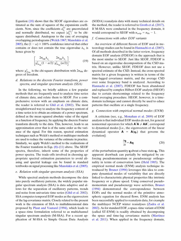
is shown in Fig. 1 (left). The distinct peaks at 365days,

183days and so on represent annual and seasonal cycles

that are, however, not of primary interest for this analysis.

Many of the climate patterns that are of interest can

better be identified by their low-rank behavior. To this

end, we define the normalizedmodal variance difference:

Dl5l12 l

2

�nblk

j51

lj

(27)

as the normalized difference in variance, between the

first and secondmode. The corresponding plot is shown

in Fig. 1 (right). Besides the annual cycle, the spectrum

exhibits a distinct peak centered around a period of

approximately 5 years. We will show in the next section

that this peak is the footprint of the ENSO and PDO. In

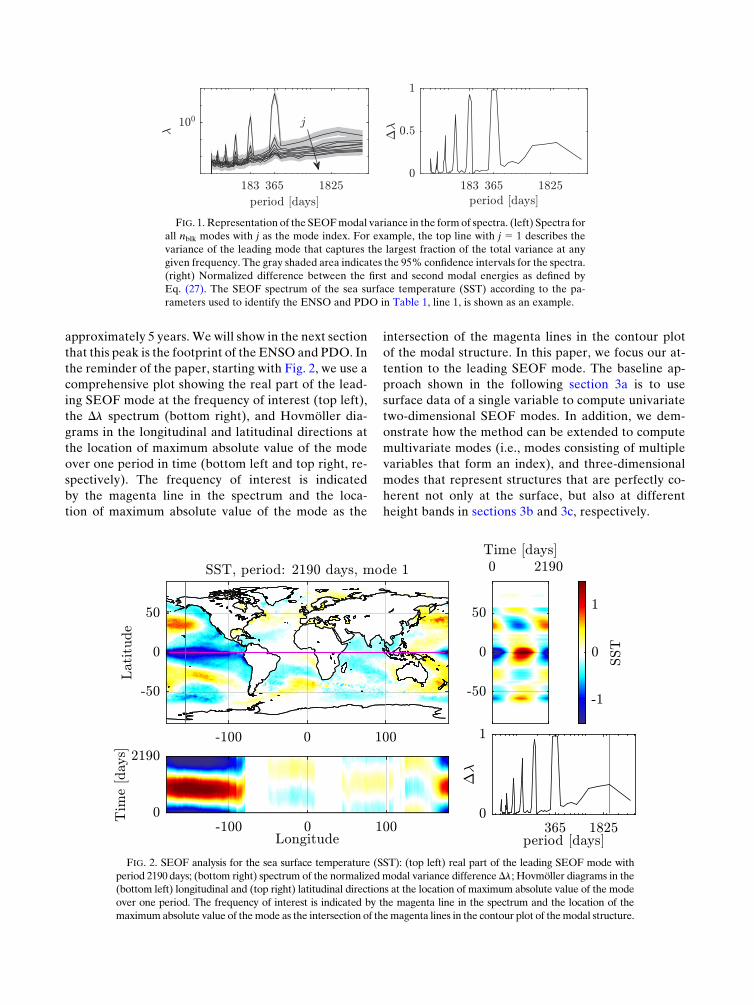
the reminder of the paper, starting with Fig. 2, we use a

comprehensive plot showing the real part of the lead-

ing SEOF mode at the frequency of interest (top left),

the Dl spectrum (bottom right), and Hovmöller dia-

grams in the longitudinal and latitudinal directions at

the location of maximum absolute value of the mode

over one period in time (bottom left and top right, re-

spectively). The frequency of interest is indicated

by the magenta line in the spectrum and the loca-

tion of maximum absolute value of the mode as the

intersection of the magenta lines in the contour plot

of the modal structure. In this paper, we focus our at-

tention to the leading SEOF mode. The baseline ap-

proach shown in the following section 3a is to use

surface data of a single variable to compute univariate

two-dimensional SEOF modes. In addition, we dem-

onstrate how the method can be extended to compute

multivariate modes (i.e., modes consisting of multiple

variables that form an index), and three-dimensional

modes that represent structures that are perfectly co-

herent not only at the surface, but also at different

height bands in sections 3b and 3c, respectively.

FIG. 1. Representation of the SEOFmodal variance in the formof spectra. (left) Spectra for

all nblk modes with j as the mode index. For example, the top line with j 5 1 describes the

variance of the leading mode that captures the largest fraction of the total variance at any

given frequency. The gray shaded area indicates the 95% confidence intervals for the spectra.

(right) Normalized difference between the first and second modal energies as defined by

Eq. (27). The SEOF spectrum of the sea surface temperature (SST) according to the pa-

rameters used to identify the ENSO and PDO in Table 1, line 1, is shown as an example.

FIG. 2. SEOF analysis for the sea surface temperature (SST): (top left) real part of the leading SEOF mode with

period 2190 days; (bottom right) spectrum of the normalized modal variance differenceDl; Hovmöller diagrams in the

(bottom left) longitudinal and (top right) latitudinal directions at the location of maximum absolute value of the mode

over one period. The frequency of interest is indicated by the magenta line in the spectrum and the location of the

maximum absolute value of themode as the intersection of themagenta lines in the contour plot of themodal structure.

a. Univariate two-dimensional data

1) EL NIÑO–SOUTHERN OSCILLATION AND LINKS

TO PACIFIC DECADAL OSCILLATION (PDO)PATTERNS

2–7-yr (ENSO) and 8–12-yr (PDO) periodicity

The El Niño–Southern Oscillation analyzed in Fig. 3

involves coupled atmospheric–ocean processes, and repre-

sents the strongest year-to-year fluctuation of the global

climate system, affecting ecosystems as well as human

activities. While it has been widely studied throughout

the past few decades, its complexity makes it difficult to

reach a full understanding of both large- and small-scale

effects of this phenomenon, as well as of its implications

on other modes of variability (Timmermann et al. 2018).

ENSO is characterized by the periodic change in winds

and sea surface temperature (SST) in the tropical eastern

Pacific Ocean, coupled with periodic air surface pressure

variation in the tropical western Pacific Ocean. The indi-

vidual ENSO periods last several months each (typically

occurring every few years) and their effects vary in intensity

and complexity (see, e.g., Trenberth 1997).

ENSO-like, the Pacific decadal oscillation is a coupled

ocean–atmosphere process, that is however, most visible in

the North Pacific region with alternating patterns of SST

[see, e.g., Mantua and Hare (2002) for further details].

Interestingly, the SEOFanalysis identifies and links both,

the anomalous patterns in the North Pacific reminiscent

of the PDOand the equatorial SST. InFig. 2, theENSOand

the PDO patterns are identified in the SST. In the SEOF

modedepicted inFig. 2, the occurrence of these twopatterns

is evident. In the normalized power spectrum, the ENSO

pattern materializes in the form of a broad crest that is

centered about a 5-yr-period peak. The spread around the

peak is in accordance with the typical ENSO variability.

The interplay between the ENSO and PDO has been

the focus of several recent studies (e.g.,Wang et al. 2014),

and has strong implications in terms of teleconnections

and global circulation patterns, among others.

2) QUASI-BIENNIAL OSCILLATION (QBO)

28–29-month periodicity

The QBO exhibits quasi-periodic reversals of the zonal-

mean zonal winds in the equatorial stratosphere between

easterlies andwesterlies with a distinct apparent downward

phase propagation of the alternating wind regimes [see,

e.g., Baldwin et al. (2001) for further details]. This mode of

variability has important implications in terms of tele-

connections with several weather patterns in the Northern

Hemisphere, including averaged zonal winds, mean sea

level pressure and tropical precipitation (Gray et al. 2018).

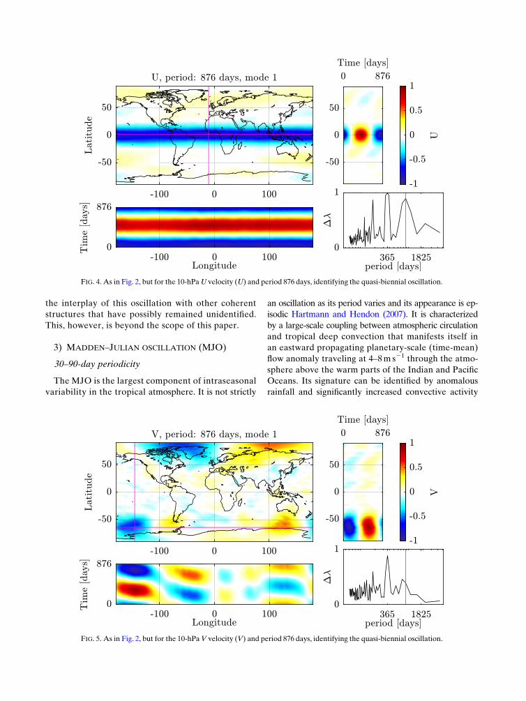
It can be seen that the QBO is most unambiguously

identified in terms of the 10-hPa U component of the

wind velocity shown in Fig. 4. The corresponding spa-

tial pattern is a clear latitudinal band in 2208&f& 208.

The 10-hPa V wind component and the mean sea level

pressure (MSL) shown in Figs. 3 and 5, respectively,

exhibit a significantly less distinct peak in the spectra

around the typical QBO period. A more comprehensive

SEOF analysis can uncover teleconnections as well as

FIG. 3. As inFig. 2, but for themean sea level pressure (MSL) andperiod 876days, identifying thequasi-biennial oscillation.

the interplay of this oscillation with other coherent

structures that have possibly remained unidentified.

This, however, is beyond the scope of this paper.

3) MADDEN–JULIAN OSCILLATION (MJO)

30–90-day periodicity

The MJO is the largest component of intraseasonal

variability in the tropical atmosphere. It is not strictly

an oscillation as its period varies and its appearance is ep-

isodic Hartmann and Hendon (2007). It is characterized

by a large-scale coupling between atmospheric circulation

and tropical deep convection that manifests itself in

an eastward propagating planetary-scale (time-mean)

flow anomaly traveling at 4–8m s21 through the atmo-

sphere above the warm parts of the Indian and Pacific

Oceans. Its signature can be identified by anomalous

rainfall and significantly increased convective activity

FIG. 5. As in Fig. 2, but for the 10-hPaV velocity (V) and period 876 days, identifying the quasi-biennial oscillation.

FIG. 4. As in Fig. 2, but for the 10-hPaU velocity (U) and period 876 days, identifying the quasi-biennial oscillation.

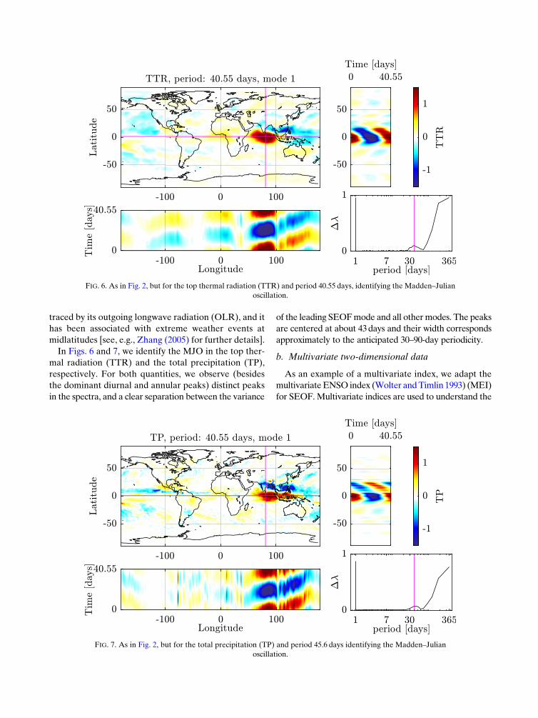
traced by its outgoing longwave radiation (OLR), and it

has been associated with extreme weather events at

midlatitudes [see, e.g., Zhang (2005) for further details].

In Figs. 6 and 7, we identify the MJO in the top ther-

mal radiation (TTR) and the total precipitation (TP),

respectively. For both quantities, we observe (besides

the dominant diurnal and annular peaks) distinct peaks

in the spectra, and a clear separation between the variance

of the leading SEOFmode and all othermodes. The peaks

are centered at about 43days and their width corresponds

approximately to the anticipated 30–90-day periodicity.

b. Multivariate two-dimensional data

As an example of a multivariate index, we adapt the

multivariateENSO index (Wolter andTimlin 1993) (MEI)

for SEOF. Multivariate indices are used to understand the

FIG. 6. As in Fig. 2, but for the top thermal radiation (TTR) and period 40.55 days, identifying the Madden–Julian

oscillation.

FIG. 7. As in Fig. 2, but for the total precipitation (TP) and period 45.6 days identifying the Madden–Julian

oscillation.

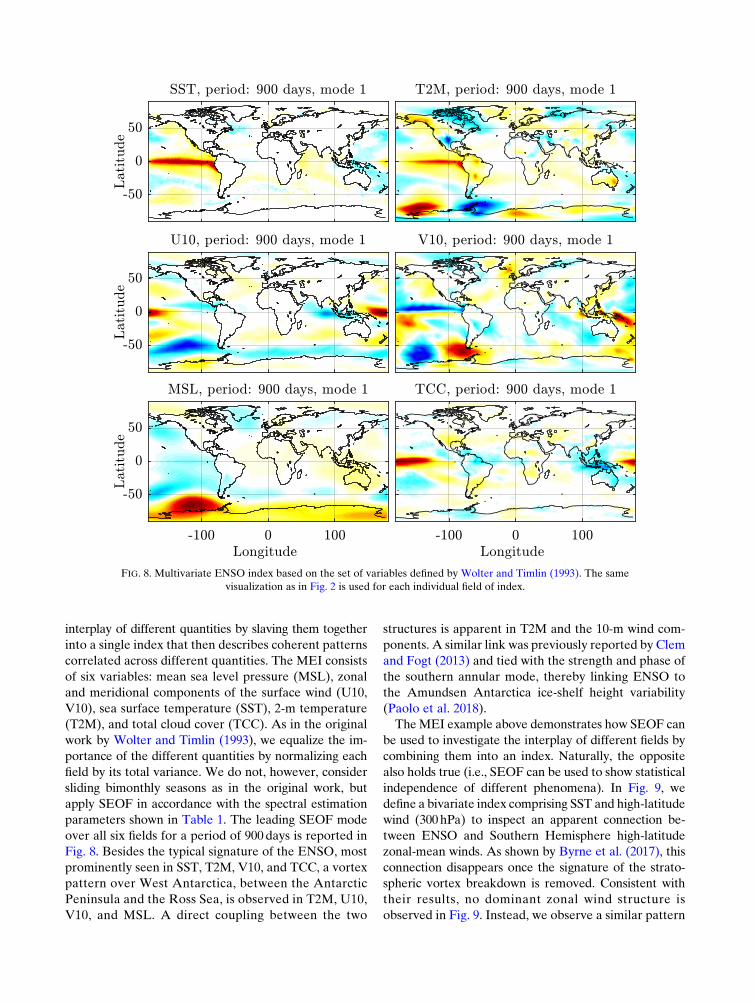
interplay of different quantities by slaving them together

into a single index that then describes coherent patterns

correlated across different quantities. The MEI consists

of six variables: mean sea level pressure (MSL), zonal

and meridional components of the surface wind (U10,

V10), sea surface temperature (SST), 2-m temperature

(T2M), and total cloud cover (TCC). As in the original

work by Wolter and Timlin (1993), we equalize the im-

portance of the different quantities by normalizing each

field by its total variance. We do not, however, consider

sliding bimonthly seasons as in the original work, but

apply SEOF in accordance with the spectral estimation

parameters shown in Table 1. The leading SEOF mode

over all six fields for a period of 900 days is reported in

Fig. 8. Besides the typical signature of the ENSO, most

prominently seen in SST, T2M, V10, and TCC, a vortex

pattern over West Antarctica, between the Antarctic

Peninsula and the Ross Sea, is observed in T2M, U10,

V10, and MSL. A direct coupling between the two

structures is apparent in T2M and the 10-m wind com-

ponents. A similar link was previously reported by Clem

and Fogt (2013) and tied with the strength and phase of

the southern annular mode, thereby linking ENSO to

the Amundsen Antarctica ice-shelf height variability

(Paolo et al. 2018).

TheMEI example above demonstrates how SEOF can

be used to investigate the interplay of different fields by

combining them into an index. Naturally, the opposite

also holds true (i.e., SEOF can be used to show statistical

independence of different phenomena). In Fig. 9, we

define a bivariate index comprising SST and high-latitude

wind (300hPa) to inspect an apparent connection be-

tween ENSO and Southern Hemisphere high-latitude

zonal-mean winds. As shown by Byrne et al. (2017), this

connection disappears once the signature of the strato-

spheric vortex breakdown is removed. Consistent with

their results, no dominant zonal wind structure is

observed in Fig. 9. Instead, we observe a similar pattern

FIG. 8. Multivariate ENSO index based on the set of variables defined by Wolter and Timlin (1993). The same

visualization as in Fig. 2 is used for each individual field of index.

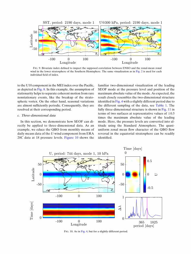
to theU10 component in theMEI index over the Pacific,

as depicted in Fig. 8. In this example, the assumption of

stationarity helps to separate coherent motion from rare

nonstationary events, like the breakup of the strato-

spheric vortex. On the other hand, seasonal variations

are almost sufficiently periodic. Consequently, they are

resolved at their corresponding period.

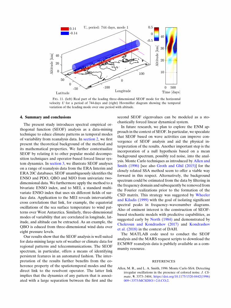
c. Three-dimensional data

In this section, we demonstrate how SEOF can di-

rectly be applied to three-dimensional data. As an

example, we educe the QBO from monthly means of

daily means data of theU-wind component from ERA

20C data at 18 pressure levels. Figure 10 shows the

familiar two-dimensional visualization of the leading

SEOF mode at the pressure level and position of the

maximum absolute value of the mode. As expected, the

result closely resembles the two-dimensional structure

identified in Fig. 4 with a slightly different period due to

the different sampling of the data, see Table 1. The

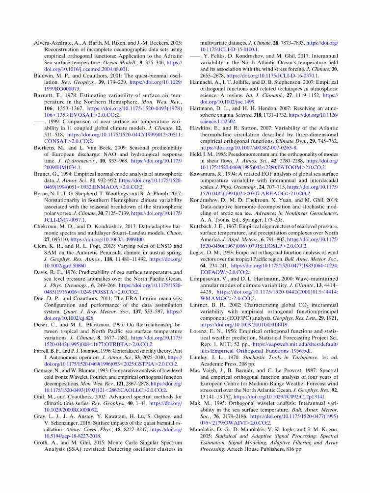
fully three-dimensional structure is shown in Fig. 11 in

terms of two surfaces at representative values of 60.5

times the maximum absolute value of the leading

mode. Here, the pressure levels are converted into al-

titude using the Standard Atmosphere. The quasi-

uniform zonal mean flow character of the QBO flow

reversal in the equatorial stratosphere can be readily

identified.

FIG. 9. Bivariate index defined to inspect the supposed correlation between ENSO and the zonal-mean zonal

wind in the lower stratosphere of the Southern Hemisphere. The same visualization as in Fig. 2 is used for each

individual field of index.

FIG. 10. As in Fig. 4, but for a slightly different period.

4. Summary and conclusions

The present study introduces spectral empirical or-

thogonal function (SEOF) analysis as a data-mining

technique to educe climate patterns as temporal modes

of variability from reanalysis data. In section 2, we first

present the theoretical background of the method and

its mathematical properties. We further contextualize

SEOF by relating it to other popular modal decompo-

sition techniques and operator-based forced linear sys-

tem dynamics. In section 3, we illustrate SEOF analyses

on a range of reanalysis data from the ERA Interim and

ERA 20C databases. SEOF unambiguously identifies the

ENSO and PDO, QBO and MJO from univariate two-

dimensional data. We furthermore apply the method to a

bivariate ENSO index, and to MEI, a standard multi-

variate ENSO index that uses six different fields of sur-

face data. Application to the MEI reveals intervariable

cross correlations that link, for example, the equatorial

oscillations of the sea surface temperature to wind pat-

terns over West Antarctica. Similarly, three-dimensional

modes of variability that are correlated in longitude, lat-

itude, and altitude can be extracted. As an example, the

QBO is educed from three-dimensional wind data over

eight pressure levels.

Our results show that the SEOF analysis is well suited

for data-mining large sets of weather or climate data for

regional patterns and telecommunications. The SEOF

spectrum, in particular, offers a means of identifying

persistent features in an automated fashion. The inter-

pretation of the results further benefits from the co-

herence property of the spatiotemporal modes and the

direct link to the resolvent operator. The latter link

implies that the dynamics of any pattern that is associ-

ated with a large separation between the first and the

second SEOF eigenvalues can be modeled as a sto-

chastically forced linear dynamical system.

In future research, we plan to explore the ENM ap-

proach in the context of SEOF. In particular, we speculate

that SEOF based on wave activities can improve con-

vergence of SEOF analysis and aid the physical in-

terpretation of the results. Another important step is the

incorporation of a null hypothesis based on a mean

background spectrum, possibly red noise, into the anal-

ysis. Monte Carlo techniques as introduced by Allen and

Smith (1996) [see also Groth and Ghil (2015)] for the

closely related SSA method seem to offer a viable way

forward in this respect. Alternatively, the background

spectrum could be estimated from the data by filtering in

the frequency domain and subsequently be removed from

the Fourier realizations prior to the formation of the

CSD matrix. This strategy was suggested by Wheeler

and Kiladis (1999) with the goal of isolating significant

spectral peaks in frequency–wavenumber diagrams.

Also of eminent interest is the construction of SEOF-

based stochastic models with predictive capabilities, as

suggested early by North (1984) and demonstrated by

Chekroun and Kondrashov (2017) and Kondrashov

et al. (2018) in the context of DAH.

The MATLAB code used to conduct the SEOF

analysis and the MARS request scripts to download the

ECMWF reanalysis data is publicly available as a com-

munity resource.

REFERENCES

Allen, M. R., and L. A. Smith, 1996: Monte Carlo SSA: Detecting

irregular oscillations in the presence of colored noise. J. Cli-

mate, 9, 3373–3404, https://doi.org/10.1175/1520-0442(1996)

009,3373:MCSDIO.2.0.CO;2.

FIG. 11. (left) Real part of the leading three-dimensional SEOF mode for the horizontal

velocity U for a period of 744 days and (right) Hovmöller diagram showing the temporal

variation of the leading mode over one period with altitude.

Alvera-Azcárate, A., A. Barth, M. Rixen, and J.-M. Beckers, 2005:

Reconstruction of incomplete oceanographic data sets using

empirical orthogonal functions: Application to the Adriatic

Sea surface temperature. Ocean Modell., 9, 325–346, https://

doi.org/10.1016/j.ocemod.2004.08.001.

Baldwin, M. P., and Coauthors, 2001: The quasi-biennial oscil-

lation. Rev. Geophys., 39, 179–229, https://doi.org/10.1029/

1999RG000073.

Barnett, T., 1978: Estimating variability of surface air tem-

perature in the Northern Hemisphere. Mon. Wea. Rev.,

106, 1353–1367, https://doi.org/10.1175/1520-0493(1978)

106,1353:EVOSAT.2.0.CO;2.

——, 1999: Comparison of near-surface air temperature vari-

ability in 11 coupled global climate models. J. Climate, 12,

511–518, https://doi.org/10.1175/1520-0442(1999)012,0511:

CONSAT.2.0.CO;2.

Bierkens, M., and L. Van Beek, 2009: Seasonal predictability

of European discharge: NAO and hydrological response

time. J. Hydrometeor., 10, 953–968, https://doi.org/10.1175/

2009JHM1034.1.

Brunet, G., 1994: Empirical normal-mode analysis of atmospheric

data. J. Atmos. Sci., 51, 932–952, https://doi.org/10.1175/1520-

0469(1994)051,0932:ENMAOA.2.0.CO;2.

Byrne, N. J., T. G. Shepherd, T. Woollings, and R. A. Plumb, 2017:

Nonstationarity in Southern Hemisphere climate variability

associated with the seasonal breakdown of the stratospheric

polar vortex. J. Climate, 30, 7125–7139, https://doi.org/10.1175/

JCLI-D-17-0097.1.

Chekroun, M. D., and D. Kondrashov, 2017: Data-adaptive har-

monic spectra and multilayer Stuart–Landau models. Chaos,

27, 093110, https://doi.org/10.1063/1.4989400.

Clem, K. R., and R. L. Fogt, 2013: Varying roles of ENSO and

SAM on the Antarctic Peninsula climate in austral spring.

J. Geophys. Res. Atmos., 118, 11 481–11 492, https://doi.org/

10.1002/jgrd.50860

Davis, R. E., 1976: Predictability of sea surface temperature and

sea level pressure anomalies over the North Pacific Ocean.

J. Phys. Oceanogr., 6, 249–266, https://doi.org/10.1175/1520-

0485(1976)006,0249:POSSTA.2.0.CO;2.

Dee, D. P., and Coauthors, 2011: The ERA-Interim reanalysis:

Configuration and performance of the data assimilation

system. Quart. J. Roy. Meteor. Soc., 137, 553–597, https://

doi.org/10.1002/qj.828.

Deser, C., and M. L. Blackmon, 1995: On the relationship be-

tween tropical and North Pacific sea surface temperature

variations. J. Climate, 8, 1677–1680, https://doi.org/10.1175/

1520-0442(1995)008,1677:OTRBTA.2.0.CO;2.

Farrell, B. F., andP. J. Ioannou, 1996:Generalized stability theory. Part

I: Autonomous operators. J. Atmos. Sci., 53, 2025–2040, https://

doi.org/10.1175/1520-0469(1996)053,2025:GSTPIA.2.0.CO;2.

Gamage,N., andW.Blumen, 1993: Comparative analysis of low-level

cold fronts:Wavelet, Fourier, and empirical orthogonal function

decompositions.Mon.Wea. Rev., 121, 2867–2878, https://doi.org/

10.1175/1520-0493(1993)121,2867:CAOLLC.2.0.CO;2.

Ghil, M., and Coauthors, 2002: Advanced spectral methods for

climatic time series. Rev. Geophys., 40, 1–41, https://doi.org/

10.1029/2000RG000092.

Gray, L. J., J. A. Anstey, Y. Kawatani, H. Lu, S. Osprey, and

V. Schenzinger, 2018: Surface impacts of the quasi biennial os-

cillation. Atmos. Chem. Phys., 18, 8227–8247, https://doi.org/

10.5194/acp-18-8227-2018.

Groth, A., and M. Ghil, 2015: Monte Carlo Singular Spectrum

Analysis (SSA) revisited: Detecting oscillator clusters in

multivariate datasets. J. Climate, 28, 7873–7893, https://doi.org/

10.1175/JCLI-D-15-0100.1.

——, Y. Feliks, D. Kondrashov, and M. Ghil, 2017: Interannual

variability in the North Atlantic Ocean’s temperature field

and its association with the wind stress forcing. J. Climate, 30,

2655–2678, https://doi.org/10.1175/JCLI-D-16-0370.1.

Hannachi, A., I. T. Jolliffe, and D. B. Stephenson, 2007: Empirical

orthogonal functions and related techniques in atmospheric

science: A review. Int. J. Climatol., 27, 1119–1152, https://

doi.org/10.1002/joc.1499.

Hartmann, D. L., and H. H. Hendon, 2007: Resolving an atmo-

spheric enigma. Science, 318, 1731–1732, https://doi.org/10.1126/

science.1152502.

Hawkins, E., and R. Sutton, 2007: Variability of the Atlantic

thermohaline circulation described by three-dimensional

empirical orthogonal functions. Climate Dyn., 29, 745–762,

https://doi.org/10.1007/s00382-007-0263-8.

Held, I. M., 1985: Pseudomomentum and the orthogonality ofmodes

in shear flows. J. Atmos. Sci., 42, 2280–2288, https://doi.org/

10.1175/1520-0469(1985)042,2280:PATOOM.2.0.CO;2.

Kawamura, R., 1994: A rotated EOF analysis of global sea surface

temperature variability with interannual and interdecadal

scales. J. Phys. Oceanogr., 24, 707–715, https://doi.org/10.1175/

1520-0485(1994)024,0707:AREAOG.2.0.CO;2.

Kondrashov, D., M. D. Chekroun, X. Yuan, and M. Ghil, 2018:

Data-adaptive harmonic decomposition and stochastic mod-

eling of arctic sea ice. Advances in Nonlinear Geosciences,

A. A. Tsonis, Ed., Springer, 179–205.

Kutzbach, J. E., 1967: Empirical eigenvectors of sea-level pressure,

surface temperature, and precipitation complexes over North

America. J. Appl. Meteor., 6, 791–802, https://doi.org/10.1175/

1520-0450(1967)006,0791:EEOSLP.2.0.CO;2.

Legler, D. M., 1983: Empirical orthogonal function analysis of wind

vectors over the tropical Pacific region.Bull. Amer.Meteor. Soc.,

64, 234–241, https://doi.org/10.1175/1520-0477(1983)064,0234:

EOFAOW.2.0.CO;2.

Limpasuvan, V., and D. L. Hartmann, 2000: Wave-maintained

annular modes of climate variability. J. Climate, 13, 4414–

4429, https://doi.org/10.1175/1520-0442(2000)013,4414:

WMAMOC.2.0.CO;2.

Lintner, B. R., 2002: Characterizing global CO2 interannual

variability with empirical orthogonal function/principal

component (EOF/PC) analysis.Geophys. Res. Lett., 29, 1921,

https://doi.org/10.1029/2001GL014419.

Lorenz, E. N., 1956: Empirical orthogonal functions and statis-

tical weather prediction. Statistical Forecasting Project Sci.

Rep. 1, MIT, 52 pp., https://eapsweb.mit.edu/sites/default/

files/Empirical_Orthogonal_Functions_1956.pdf.

Lumley, J. L., 1970: Stochastic Tools in Turbulence. 1st ed.

Academic Press, 208 pp.

Mac Veigh, J., B. Barnier, and C. Le Provost, 1987: Spectral

and empirical orthogonal function analysis of four years of

European Centre for Medium-Range Weather Forecast wind

stress curl over theNorthAtlanticOcean. J. Geophys. Res., 92,

13 141–13 152, https://doi.org/10.1029/JC092iC12p13141.

Mak, M., 1995: Orthogonal wavelet analysis: Interannual vari-

ability in the sea surface temperature. Bull. Amer. Meteor.

Soc., 76, 2179–2186, https://doi.org/10.1175/1520-0477(1995)

076,2179:OWAIVI.2.0.CO;2.

Manolakis, D. G., D. Manolakis, V. K. Ingle, and S. M. Kogon,

2005: Statistical and Adaptive Signal Processing: Spectral

Estimation, Signal Modeling, Adaptive Filtering and Array

Processing. Artech House Publishers, 816 pp.

Mantua, N. J., and S. R. Hare, 2002: The Pacific decadal oscillation.

J. Oceanogr., 58, 35–44, https://doi.org/10.1023/A:1015820616384.

Marshall, G. J., 2003: Trends in the Southern Annular Mode from

observations and reanalyses. J. Climate, 16, 4134–4143, https://

doi.org/10.1175/1520-0442(2003)016,4134:TITSAM.2.0.CO;2.

Martinez, Y., G. Brunet, M. K. Yau, and X. Wang, 2011: On the

dynamics of concentric eyewall genesis: Space–time empirical

normal modes diagnosis. J. Atmos. Sci., 68, 457–476, https://

doi.org/10.1175/2010JAS3501.1.

Matsuo, T., and J. M. Forbes, 2010: Principal modes of thermo-

spheric density variability: Empirical orthogonal function

analysis of CHAMP 2001–2008 data. J. Geophys. Res., 115,

A07309, https://doi.org/10.1029/2009JA015109.

Miller, J. K., and R. G. Dean, 2007a: Shoreline variability via

empirical orthogonal function analysis: Part I temporal and

spatial characteristics. Coastal Eng., 54, 111–131, https://doi.org/

10.1016/j.coastaleng.2006.08.013.

——, and ——, 2007b: Shoreline variability via empirical orthog-

onal function analysis: Part II relationship to nearshore con-

ditions. Coastal Eng., 54, 133–150, https://doi.org/10.1016/

j.coastaleng.2006.08.014.

Min, S.-K., X. Zhang, F.W. Zwiers, andG. C.Hegerl, 2011: Human

contribution to more-intense precipitation extremes. Nature,

470, 378–381, https://doi.org/10.1038/nature09763.Mo, K. C., 2000: Relationships between low-frequency variability

in the Southern Hemisphere and sea surface temperature

anomalies. J. Climate, 13, 3599–3610, https://doi.org/10.1175/

1520-0442(2000)013,3599:RBLFVI.2.0.CO;2.

Monahan, A. H., J. C. Fyfe, M. H. P. Ambaum, D. B. Stephenson,

and G. R. North, 2009: Empirical orthogonal functions: The

medium is the message. J. Climate, 22, 6501–6514, https://

doi.org/10.1175/2009JCLI3062.1.

Mu, Q., C. S. Jackson, and P. L. Stoffa, 2004: A multivariate

empirical-orthogonal-function-basedmeasure of climate model

performance. J. Geophys. Res., 109, D15101, https://doi.org/

10.1029/2004JD004584.

Navarra, A., and V. Simoncini, 2010: A Guide to Empirical

Orthogonal Functions for Climate Data Analysis. Springer

Science & Business Media, 151 pp.

Newman, M., G. P. Compo, and M. A. Alexander, 2003: ENSO-

forced variability of the Pacific decadal oscillation. J. Climate, 16,

3853–3857, https://doi.org/10.1175/1520-0442(2003)016,3853:

EVOTPD.2.0.CO;2.

North, G. R., 1984: Empirical orthogonal functions and normal

modes. J. Atmos. Sci., 41, 879–887, https://doi.org/10.1175/

1520-0469(1984)041,0879:EOFANM.2.0.CO;2.

Obukhov, A., 1947: Statistically homogeneous fields on a sphere.

Uspekhi Mat. Nauk, 2 (2), 196–198.

Palmer, T. N., and D. L. Anderson, 1994: The prospects

for seasonal forecasting—A review paper. Quart. J.

Roy. Meteor. Soc., 120, 755–793, https://doi.org/10.1002/

QJ.49712051802.

Paolo, F., L. Padman, H. Fricker, S. Adusumilli, S. Howard, and

M.Siegfried, 2018:ResponseofPacific-sectorAntarctic ice shelves

to the El Niño/Southern Oscillation. Nat. Geosci., 11, 121–126,

https://doi.org/10.1038/s41561-017-0033-0.

Plaut, G., and R. Vautard, 1994: Spells of low-frequency oscillations

andweather regimes in theNorthernHemisphere. J. Atmos. Sci.,

51, 210–236, https://doi.org/10.1175/1520-0469(1994)051,0210:

SOLFOA.2.0.CO;2.

Poli, P., and Coauthors, 2016: ERA-20C: An atmospheric re-

analysis of the twentieth century. J. Climate, 29, 4083–4097,

https://doi.org/10.1175/JCLI-D-15-0556.1.

Pritchard, M. S., and R. C. Somerville, 2009: Empirical orthogonal

function analysis of the diurnal cycle of precipitation in a

multi-scale climate model. Geophys. Res. Lett., 36, L05812,

https://doi.org/10.1029/2008GL036964.

Sardeshmukh, P. D., and P. Sura, 2009: Reconciling non-Gaussian

climate statisticswith linear dynamics. J.Climate, 22, 1193–1207,

https://doi.org/10.1175/2008JCLI2358.1.

Schmidt, E., 1907: Zur theorie der linearen und nicht linearen in-

tegralgleichungen zweite abhandlung.Math. Ann., 64, 161–174,

https://doi.org/10.1007/BF01449890.

Schmidt, O. T., and A. Towne, 2019: An efficient streaming al-

gorithm for spectral proper orthogonal decomposition.

Comput. Phys. Commun., 237, 98–109, https://doi.org/

10.1016/j.cpc.2018.11.009.

——, ——, G. Rigas, T. Colonius, and G. A. Brès, 2018: Spectralanalysis of jet turbulence. J. FluidMech., 855, 953–982, https://

doi.org/10.1017/jfm.2018.675.

Servain, J., and D. M. Legler, 1986: Empirical orthogonal function

analyses of tropical Atlantic sea surface temperature and wind

stress: 1964–1979. J. Geophys. Res., 91, 14 181–14 191, https://

doi.org/10.1029/JC091iC12p14181.

Sirovich, L., 1987: Turbulence and the dynamics of coherent

structures. Quart. Appl. Math., 45, 561–571, https://doi.org/

10.1090/qam/910462.

——, and R. Everson, 1992: Management and analysis of large

scientific datasets. Int. J. Supercomput. Appl., 6, 50–68, https://

doi.org/10.1177/109434209200600104.

Smith, T. M., R. W. Reynolds, R. E. Livezey, and D. C. Stokes, 1996:

Reconstruction of historical sea surface temperatures using em-

pirical orthogonal functions. J. Climate, 9, 1403–1420, https://

doi.org/10.1175/1520-0442(1996)009,1403:ROHSST.2.0.CO;2.

Thompson, D. W., and J. M. Wallace, 2000: Annular modes in

the extratropical circulation. Part I: Month-to-month var-

iability. J. Climate, 13, 1000–1016, https://doi.org/10.1175/

1520-0442(2000)013,1000:AMITEC.2.0.CO;2.

Timmermann, A., and Coauthors, 2018: El Niño–Southern Oscil-

lation complexity. Nature, 559, 535–545, https://doi.org/

10.1038/s41586-018-0252-6.

Towne, A., O. T. Schmidt, and T. Colonius, 2018: Spectral proper

orthogonal decomposition and its relationship to dynamic

mode decomposition and resolvent analysis. J. Fluid Mech.,

847, 821–867, https://doi.org/10.1017/jfm.2018.283.

Trenberth, K. E., 1997: The definition of El Niño. Bull. Amer.

Meteor. Soc., 78, 2771–2777, https://doi.org/10.1175/1520-

0477(1997)078,2771:TDOENO.2.0.CO;2.

Wang, B., and S.-I. An, 2005: A method for detecting season-

dependent modes of climate variability: S-EOF analysis.

Geophys. Res. Lett., 32, L15710, https://doi.org/10.1029/

2005GL022709.

——, J.-Y. Lee, and B. Xiang, 2015: Asian summer monsoon

rainfall predictability: A predictable mode analysis. Climate

Dyn., 44, 61–74, https://doi.org/10.1007/s00382-014-2218-1.

Wang, S., J. Huang, Y. He, andY. Guan, 2014: Combined effects of

the Pacific decadal oscillation and El Nino–Southern Oscilla-

tion on global land dry–wet changes. Sci. Rep., 4, 6651, https://

doi.org/10.1038/srep06651.

Weare, B. C., and R. Newell, 1977: Empirical orthogonal analysis of

AtlanticOcean surface temperatures.Quart. J. Roy.Meteor. Soc.,

103, 467–478, https://doi.org/10.1002/qj.49710343707.

——, and J. S. Nasstrom, 1982: Examples of extended empirical

orthogonal function analyses. Mon. Wea. Rev., 110, 481–

485, https://doi.org/10.1175/1520-0493(1982)110,0481:

EOEEOF.2.0.CO;2.

——,A. R. Navato, and R. E. Newell, 1976: Empirical orthogonal

analysis of Pacific sea surface temperatures. J. Phys. Oce-

anogr., 6, 671–678, https://doi.org/10.1175/1520-0485(1976)

006,0671:EOAOPS.2.0.CO;2.

Welch, P., 1967: The use of fast Fourier transform for the estima-

tion of power spectra: Amethod based on time averaging over

short, modified periodograms. IEEE Trans. Audio Electro-

acoust., 15, 70–73, https://doi.org/10.1109/TAU.1967.1161901.

Wheeler, M., and G. N. Kiladis, 1999: Convectively coupled

equatorial waves: Analysis of clouds and temperature in the

wavenumber–frequency domain. J. Atmos. Sci., 56, 374–399,

https://doi.org/10.1175/1520-0469(1999)056,0374:CCEWAO.2.0.CO;2.

Wolter, K., and M. S. Timlin, 1993: Monitoring ENSO in

COADS with a seasonally adjusted principal component

index. Proc. 17th Climate Diagnostics Workshop, Norman,

OK, CIMMS, 52–57.

Wu, Z., B. Wang, J. Li, and F.-F. Jin, 2009: An empirical seasonal

prediction model of the East Asian summer monsoon using

ENSO and NAO. J. Geophys. Res., 114, D18120, https://

doi.org/10.1029/2009JD011733.

Zadra, A., G. Brunet, and J. Derome, 2002: An empirical normal

mode diagnostic algorithm applied to NCEP reanalyses.

J. Atmos. Sci., 59, 2811–2829, https://doi.org/10.1175/1520-

0469(2002)059,2811:AENMDA.2.0.CO;2.

Zhang, C., 2005: Madden-Julian Oscillation. Rev. Geophys., 43,

RG2003, https://doi.org/10.1029/2004RG000158.

Zhang, Y., J. M. Wallace, and D. S. Battisti, 1997: ENSO-like inter-

decadal variability: 1900–93. J. Climate, 10, 1004–1020, https://

doi.org/10.1175/1520-0442(1997)010,1004:ELIV.2.0.CO;2.