Embed Size (px)
Citation preview

Spectral Library ToolRelease 1.1.3
Dec 13, 2020


Contents
1 Installation Instructions 31.1 Installation of QGIS Plugin . . . . . . . . . . . . . . . . . . . . . . . . . . . . . . . . . . . . . . . 31.2 Installation of the python package . . . . . . . . . . . . . . . . . . . . . . . . . . . . . . . . . . . . 3
2 User Guide 52.1 Creating/Editing a Spectral Library . . . . . . . . . . . . . . . . . . . . . . . . . . . . . . . . . . . 52.2 Spectral Library Optimization . . . . . . . . . . . . . . . . . . . . . . . . . . . . . . . . . . . . . . 8
3 Exercises 273.1 Exercise Brussels . . . . . . . . . . . . . . . . . . . . . . . . . . . . . . . . . . . . . . . . . . . . . 273.2 Exercise Santa Barbara . . . . . . . . . . . . . . . . . . . . . . . . . . . . . . . . . . . . . . . . . . 37
4 Spectral Library Tool API 514.1 Spectral Library Optimization . . . . . . . . . . . . . . . . . . . . . . . . . . . . . . . . . . . . . . 51
5 About The Spectral Library Tool 615.1 Indexes . . . . . . . . . . . . . . . . . . . . . . . . . . . . . . . . . . . . . . . . . . . . . . . . . . 62
Bibliography 63
Python Module Index 67
Index 69
i

ii
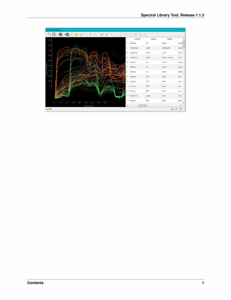
Spectral Library Tool, Release 1.1.3
Contents 1

Spectral Library Tool, Release 1.1.3
2 Contents
CHAPTER 1
Installation Instructions
For issues, bugs, proposals or remarks, visit the issue tracker.
1.1 Installation of QGIS Plugin
The plugin is available in the QGIS Python Plugins Repository:
Plugins menu > Manage and install plugins... > All > Search for 'Spectral Library Tool→˓'
Alternatively, you can download the latest stable distribution (spectral-libraries-x-qgis.zip) and install the plugin man-ually:
Plugins menu > Manage and install plugins... > Install from ZIP > Browse to the zip→˓file > Click *Install plugin*.
Note: The plugin is build for QGIS Version 3.6 and up. We recommend to use QGIS version 3.10. The plugin hasbeen tested on Windows 10.0, Ubuntu 16.04 and Raspbian GNU/Linux 10 (buster)
1.2 Installation of the python package
Open a shell by running the following batch script (adapt to match with your installation):
::QGIS installation folderset OSGEO4W_ROOT=C:\OSGeo4W64
::set defaults, clean path, load OSGeo4W modules (incrementally)call %OSGEO4W_ROOT%\bin\o4w_env.bat
(continues on next page)
3

Spectral Library Tool, Release 1.1.3
(continued from previous page)
call qt5_env.batcall py3_env.bat
::lines taken from python-qgis.batset QGIS_PREFIX_PATH=%OSGEO4W_ROOT%\apps\qgisset PATH=%QGIS_PREFIX_PATH%\bin;%PATH%
::make PyQGIS packages available to Pythonset PYTHONPATH=%QGIS_PREFIX_PATH%\python;%PYTHONPATH%
:: GDAL Configuration (https://trac.osgeo.org/gdal/wiki/ConfigOptions):: Set VSI cache to be used as buffer, see #6448 andset GDAL_FILENAME_IS_UTF8=YESset VSI_CACHE=TRUEset VSI_CACHE_SIZE=1000000set QT_PLUGIN_PATH=%QGIS_PREFIX_PATH%\qtplugins;%OSGEO4W_ROOT%\apps\qt5\plugins
::enable/disable QGIS debug messagesset QGIS_DEBUG=1
::open the OSGeo4W Shell@echo on@if [%1]==[] (echo run o-help for a list of available commands & cmd.exe /k) else→˓(cmd /c "%*")
For command-line interface and stand-alone usage, install the python package with pip:
pip install spectral-libraries
For offline installation, you can download the latest stable distribution (spectral-libraries-x.tar.gz) and
C:\WINDOWS\system32>cd C:\Users\UserName\DownloadsC:\Users\UserName\Downloads>pip install spectral-libraries-x.tar.gz
4 Chapter 1. Installation Instructions

CHAPTER 2
User Guide
The Spectral Library Tools can be used in several ways:
1. As a plugin in QGIS
2. As a command line interface in a terminal
3. Adapting the code to fulfil very specific needs
For the last option, we refer the user to the code repository and the API at the end of this document.
For issues, bugs, proposals or remarks, visit the issue tracker.
2.1 Creating/Editing a Spectral Library
So far, QGIS has no functionality for creating, viewing or editing spectral libraries. For that reason, we had to buildthis tool ourselves. It has several functions:
• Create a Spectral Library by manually selecting spectra from an image
• Create a Spectral Library by using Regions Of Interest (polygons/points)
• Open and inspect a Spectral Library
• Edit the metadata of a Spectral Library
• Remove profiles from the Spectral Library
• . . .
It speaks for itself that a thorough understanding of the research area is required to be able to build a Spectral Libraryfrom it.
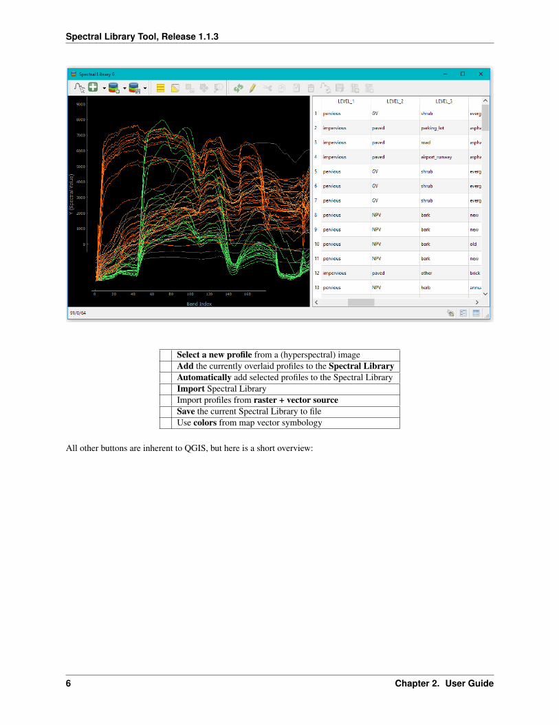
The table below gives a short overview of all Spectral Library specific buttons and their function:
5
Spectral Library Tool, Release 1.1.3
Select a new profile from a (hyperspectral) imageAdd the currently overlaid profiles to the Spectral LibraryAutomatically add selected profiles to the Spectral LibraryImport Spectral LibraryImport profiles from raster + vector sourceSave the current Spectral Library to fileUse colors from map vector symbology
All other buttons are inherent to QGIS, but here is a short overview:
6 Chapter 2. User Guide

Spectral Library Tool, Release 1.1.3
Toggle editing modeToggle multi-edit modeSave editsReload the tableAdd featureDelete selected featuresCut selected rows to clipboardCopy selected rows to clipboardPaste features from clipboardSelect features using an expressionSelect allInvert selectionDeselect allMove selection to topSelect/filter features using formPan map to the selected rowsZoom map to the selected rowsNew fieldDelete fieldConditional formattingActionsForm ViewTable ViewShow Spectral Library Properties
Note: This is a highly interactive tool and has no command line equivalent.
2.1.1 Create Spectral Library manually
In order to select spectra from an image, first load an hyperspectral image in QGIS.
• Toggle the Select Profile button .
• Click on a random pixel in the image to view a profile in the plot window. This profile is not automaticallykept, and you can click as many times as you want in the image, until you find a good profile.
• Click on the Add button to add the last profile to your Spectral Library.
• If you check the Auto button all selected profiles are automatically added to the spectral library.
• To remove a profile, select it in the attribute table and use the Delete button . In order to do so, you must firsttoggle editing mode and afterwards save your edits by clicking again on .
• You can now edit the profile metadata, add or remove non-compulsory fields and zoom/pan to your selection onthe image.
• Use the settings tool to change the colors of your profiles (according to a metadata element).
Hint: You can view a subset of your data by only setting layer properties for a subset of classes! The spectral librarybehaves like a point shape file and so the styling behaves accordingly.
2.1. Creating/Editing a Spectral Library 7
Spectral Library Tool, Release 1.1.3
2.1.2 Create Spectral Library from ROI’s
To start with this step, you need a ROI (Regions Of Interest) file. This is a QGIS Vector Layer, with each featurerepresenting an unmixing class (e.g. Pine trees). These classes, and other metadata, should be included in the attributetable.
• Make sure both the image and ROI file are open in QGIS.
• Click on Import profiles from raster + vector source : a small popup window will ask you to select the correctraster and vector files. The All touched options allows the user to choose between importing only pixels that liecompletely within the ROI’s, or also import pixels that are partly touched by the ROI’s boundaries.
• You can now edit the profile metadata, add or remove non-compulsory fields and zoom/pan to the selection onthe image.
Note: A Spectral Library will copy the attribute table of the ROI Vector Layer, it is therefore essential that it does notcontain the following protected fields: ‘fid’, ‘name’, ‘source’, ‘values’ or ‘style’.
The attribute table of the ROI Vector Layer must contain an ‘ID’ field (spelled with all capitals) with unique integervalues.
2.1.3 Open existing Spectral Library
To open an existing Spectral Library, use the Open Library button .
2.1.4 Save Spectral Library to file
To save the current Spectral Library use the Save Library button .
Note: All changes made to the Spectral Library exist in memory only, until they are saved to file.
ACKNOWLEDGMENTS
This user guide is very loosely based on the VIPER Tools 2.0 user guide (UC Santa Barbara, VIPER Lab): Roberts,D. A., Halligan, K., Dennison, P., Dudley, K., Somers, B., Crabbe, A., 2018, Viper Tools User Manual, Version 2, 91pp.
The Spectral Library tool was created for the most part at HU Berlin, by B. Jakimow. More information on the sourcecode: https://bitbucket.org/jakimowb/qgispluginsupport.
For issues, bugs, proposals or remarks, visit the issue tracker.
2.2 Spectral Library Optimization
The Spectral Library Tool includes three basic library pruning techniques: EMC, IES and CRES. EMC and IES relyon a square array. This is implemented in the background, however the option is left to the user to explore this squarearray, in order to get a better understanding of the inner workings of IES and EMC.
8 Chapter 2. User Guide
Spectral Library Tool, Release 1.1.3
2.2.1 Square Array
A square array is a way of storing how a specific endmember performs when used to unmix all other spectra in thesame library.
A square array is an image of n by n pixels, with n being the number of spectra in the Spectral Library. In this squarearray, a row corresponds to a spectrum (row = model) used to unmix all other spectra in the library (columns).
The square array is used to store metrics needed for EAR, MASA, CoB and IES. The original format of the squarearray was proposed by Roberts et al. [Roberts1997] and included in several theses published at UCSB ([Gardner1997],[Halligan2002]).
Square arrays are stored as an ENVI image, with the following possible bands: RMSE, Spectral Angle, EndmemberFraction, Shade Fraction and a ‘Constrained’ band which indicates if the model met the constraints used.
The diagonal represents each spectrum modelling itself and is meaningless so it has been zeroed out for all outputbands.
A detailed description of the Square Array Output Bands
RMSE
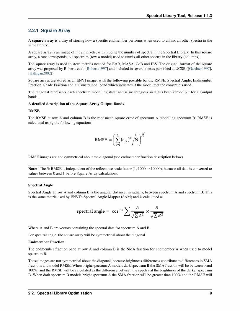
The RMSE at row A and column B is the root mean square error of spectrum A modelling spectrum B. RMSE iscalculated using the following equation:
RMSE images are not symmetrical about the diagonal (see endmember fraction description below).
Note: The % RMSE is independent of the reflectance scale factor (1, 1000 or 10000), because all data is converted tovalues between 0 and 1 before Square Array calculations.
Spectral Angle
Spectral Angle at row A and column B is the angular distance, in radians, between spectrum A and spectrum B. Thisis the same metric used by ENVI’s Spectral Angle Mapper (SAM) and is calculated as:
Where A and B are vectors containing the spectral data for spectrum A and B
For spectral angle, the square array will be symmetrical about the diagonal.
Endmember Fraction
The endmember fraction band at row A and column B is the SMA fraction for endmember A when used to modelspectrum B.
These images are not symmetrical about the diagonal, because brightness differences contribute to differences in SMAfractions and model RMSE. When bright spectrum A models dark spectrum B the SMA fraction will be between 0 and100%, and the RMSE will be calculated as the difference between the spectra at the brightness of the darker spectrumB. When dark spectrum B models bright spectrum A the SMA fraction will be greater than 100% and the RMSE will
2.2. Spectral Library Optimization 9

Spectral Library Tool, Release 1.1.3
be calculated from the difference between the spectra at the brightness of the brighter spectrum A, and thus will be alarger RMSE than the previous case.
Shade Fraction
The shade fraction at row A and column B is the SMA shade fraction for endmember A when used to model spectrumB. It is calculated as 1 minus the endmember fraction, and is included to allow for shade thresholding in the EMCcalculations.
Constraint Code
When calculating the fractions and RMSE, constraints can be used.
1. Unconstrained: It is allowed to have super positive (>100%) or negative (<0%) fractions or high RMSE values.There will be no ‘constraints’ band in the output.
2. Constrained, non-reset: Thresholds can be set for minimum and maximum fractions and for RMSE. When eitherthe fractions or the RMSE are exceeded, a value is stored in the ‘constraints’ band (see below). The fractionsand RMSE themselves stay unchanged.
Default values of -0.05, 1.05 and 0.025 for minimum fraction, maximum fraction and RMSE threshold, respec-tively, represent values used in the literature ([Halligan2002], [Roberts2003]).
The minimum fraction constraint cannot be set below -0.50, the maximum fraction constraint cannot exceed1.50, and the maximum RMSE constraint cannot exceed 0.10.
3. Constrained, reset: When fractions exceed the constraint, the fractions in the output are reset to the threshold val-ues. The RMSE is then calculated with these new fraction values instead of the original ones. The ‘constraints’band now stores different values.
This is useful for allowing models with very good fit to be included despite being slightly too dark. For example,spectrum A might be a well-fit spectrum for modelling spectrum B, but would produce a fraction of 106% (1.06)because it is darker than spectrum B. If running in non-reset mode with the maximum allowable fraction set to105% (1.05), this model would be excluded completely because it exceeds the threshold. In reset mode thismodel would be run forcing the bright endmember to have a 105% fraction. The resulting RMSE would beslightly higher (due to a slight underestimate of the bright endmember fraction) but would not be excluded. Itmay even be possible that spectrum A will produce the lowest EAR value for the library, suggesting it is anoptimal endmember despite the fact that it is fairly dark.
An overview of the possible values of the constraints band.
• 0 = no constraint breach
• 1 = fraction constraint breach + fraction reset + no RMSE constraint breach
• 2 = fraction constraint breach + no fraction reset + no RMSE constraint breach
• 3 = no fraction constraint breach + RMSE constraint breach
• 4 = fraction constraint breach + fraction reset + RMSE constraint breach
• 5 = fraction constraint breach + no fraction reset + RMSE constraint breach
QGIS GUI
Note: A square array is required for IES and EMC. EMC requires at least the RMSE and Spectral Angle bands. IESrequires the RMSE and Constraints bands.
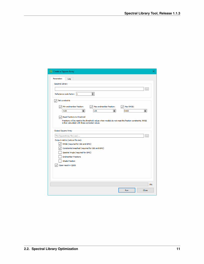
1. Select the input spectral library. Note that this library must have metadata attached to it and it is best sorted in away to assist interpretation of the square array.
2. The reflectance scale factor is automatically detected.
10 Chapter 2. User Guide
Spectral Library Tool, Release 1.1.3
2.2. Spectral Library Optimization 11
Spectral Library Tool, Release 1.1.3
Note: Spectral data can be saved to file as reflectance values (i.e. values between 0 and 1) or thedata can be multiplied by a scale factor (usually by 1000 or 10000). This is done to be able to storethe data as integer values (no comma’s), because integers require less memory. Although this is moreefficient storage-wise, it has as a result we have to divide the data values again before processing.
The software tries to auto detect this scale factor, but does not always succeed. Double check thisvalue before continuing.
3. Select if you want to use constraints for the SMA algorithm or not.
• Deselect the constraints-box to calculate the fraction and RMSE metrics without constraints. There willbe no ‘constraints’ band in the output.
• Select the constraints-box to calculate the fraction and RMSE metrics with constraints. Thresholds can beset for minimum and maximum fractions and for RMSE.
• Select or deselect the ‘reset’ box to use the constraints in reset mode or non-reset mode.
4. Select an output filename. A default name is created for you with the structure libraryName_sq.sqr. Optionally,you can add the constraint parameters. Example: name_-5_105_2pt5_sq.sqr for constraints of -5%, 105% and2.5%.
5. Select the output metrics of your choice: RMSE, Fraction, Shade Fraction, Spectral Angle and Constraints
Issue Tracker:
For issues, bugs, proposals or remarks, visit the issue tracker.
Command Line Interface
The main command is:
>square
Use -h or --help to list all possible arguments:
>square -h
Only the spectral library file is a required argument. An example:
>square "C:\Users\...\Data\spectral_library.sli"
All the other inputs are optional. Use --reflectance-scale to set the reflectance scale factor. It can also beautomatically derived from the library image as 1, 1 000 or 10 000:
>square "C:\Users\...\Data\spectral_library.sli" --reflectance-scale 255
By default, the constraints are set at -0.05 (minimum fraction), 1.05 (maximum fraction) and 0.025 (maximumRMSE). Use --min-fraction, --max-fraction and --max-rmse arguments to change these values. Toset no constraint for a given variable, use the value -9999. To use no constraints at all, use the argument -u or--unconstrained:
>square "C:\Users\...\Data\spectral_library.sli" --max-fraction 1.10 --max-rmse -9999>square "C:\Users\...\Data\spectral_library.sli" -u
By default, the constraints are used in reset mode (see explanations before). To turn this option off, use the argument-r or --reset-off:
12 Chapter 2. User Guide
Spectral Library Tool, Release 1.1.3
>square "C:\Users\...\Data\spectral_library.sli" -r
By default, the output file is stored in the same folder as the input file, with the extension ‘_sq.sqr’. To select anotherfile or another location, use the argument -o or --output:
>square "C:\Users\...\Data\spectral_library.sli" -o "C:\Users\...\Desktop\square_→˓array.sqr"
By default, the following metrics are added to the output: RMSE and Constraints. The Fractions, Shade Frac-tion and Spectral Angle are not included by default. Use the following arguments are to reverse these set-tings: --exclude-rmse, --exclude-constraints, --include-fractions, --include-shade,--include-angle:
>square "C:\Users\...\Data\spectral_library.sli" --include-fractions --include-angle
Issue Tracker:
For issues, bugs, proposals or remarks, visit the issue tracker.
2.2.2 EAR, MASA, CoB (EMC)
We use the Square Array to determine which spectra within a group of spectra are most representative of their classwhile covering the range of variability within the class. There are three approaches to do this:
Count based Endmember selection (CoB) was first proposed by Roberts et al. [Roberts2003]. Optimal endmembersare selected as those members of a library that model the greatest number of spectra within their class. Candidatemodels are assessed by whether they meet fraction and RMSE constraints when unmixing other spectra in the library(stored in the Square Array constraints band).
• The metric in_CoB stores the total number of spectra modelled within the class.
• The metric out_CoB stores the total number of spectra modelled outside of the class
The optimum model is selected as the one that has the highest in_CoB value. Note that ties are not split in this process,so several spectra can have the same in_CoB value.
To determine additional CoB selections, the Spectral Library Tool implements the approach described by Clark[Clark2005]: once an initial optimal spectrum (or spectra, in the case of ties) is selected, all members of the spec-tral library that were successfully modelled by this spectrum/spectra are culled from the list of candidate CoB spectra.After culling, a second tier in_CoB is calculated and a second tier, optimal spectrum/spectra is selected. This processcontinues until all candidate spectra have been eliminated, either by being selected as an optimal spectrum or by beingmodelled by an optimal spectrum.
Out_CoB provides a measure of confusion between classes, with a high value suggesting significant confusion betweenclasses. Ideally, the perfect spectrum will only model members of its class, and not model members outside of its class.This model would have a high in_CoB, but low out_CoB.
To assess the generality of a spectrum we include a third performance metric, the Count Based Index (CoBI)[Clark2005]. CoBI is the ratio of in_CoB to out_CoB with the denominator multiplied by the number of spectrawithin a class.
Thus a high CoBI and a high in_CoB represents an excellent choice (A specialist as described by Roberts et al.[Roberts1997]. A high CoBI and moderately low in_CoB may also be a good candidate because it captures a memberof a class that is spectrally unique, even if it is not well represented in the library. Low values of CoBI would only beacceptable if they were paired with a high in_CoB (Generalists).
Endmember Average RMSE (EAR) was first proposed by Dennison and Roberts [Dennison2003] as a means oflocating spectra within a class that provide the best fit when modelling that class. EAR is the average RMSE produced
2.2. Spectral Library Optimization 13

Spectral Library Tool, Release 1.1.3
by a spectrum when it is used to model all other members of the same class. The optimum spectrum would be the onethat produces the lowest average RMSE.
Minimum Average Spectral Angle (MASA) [Dennison2004] is similar to EAR in that it is designed to select spectrawith the best average fit within a class. It differs from EAR in that the measure of fit used is the spectral angle, not theRMSE.
MASA within a class is calculated as the average spectral angle between a candidate model and all other spectra withinthe same class. The best MASA candidate produces the lowest average spectral angle.
EAR and MASA are conceptually very similar. However, the optimum endmember selected by each metric willdepend on the overall brightness of the library. For example, for dark objects, subtle spectral differences between thereference and non-reference spectra could result in a fairly large spectral angle. At the same time, these subtle spectraldifferences would result in a small RMSE. The net result is that MASA will be far more sensitive to spectral differencesfor dark objects. For bright objects, the opposite is true. In this case, even a fairly large spectral feature may producea small difference in spectral angle, but a large difference in RMSE, and EAR would be more sensitive to spectraldifferences. For further discussion of the differences between RMSE and spectral angle as metrics of spectral fit seeDennison et al [Dennison2004]. Despite differing sensitivities for darker and brighter endmembers, one endmemberwill frequently possess both the minimum EAR and MASA values.
Note: The strength of any particular selection technique will vary with the metadata field. For example, whereas EARor MASA may outperform CoB for homogeneous selection criteria, such as dominant, CoB may outperform thesemeasures for heterogeneous selection criteria, such as impervious/pervious. Calculating the EMC file is also criticalwhen choosing the hierarchical level for your selections. For example, if a user were most interested in separatingimpervious from pervious surfaces, they might opt to sort on impervious/pervious when creating the EMC file. Adifferent user might be interested in separating urban materials, and thus would sort on the material scale.
QGIS GUI
1. Select the input spectral library. Note that this library must have metadata attached to it and it is best sorted in away to assist interpretation of the square array.
2. The reflectance scale factor is automatically detected.
Note: Spectral data can be saved to file as reflectance values (i.e. values between 0 and 1) or thedata can be multiplied by a scale factor (usually by 1000 or 10000). This is done to be able to storethe data as integer values (no comma’s), because integers require less memory. Although this is moreefficient storage-wise, it has as a result we have to divide the data values again before processing.
The software tries to auto detect this scale factor, but does not always succeed. Double check thisvalue before continuing.
3. Select the metadata element that divides the spectra in the library into classes.
4. Select if you want to use constraints for the SMA algorithm or not.
• Deselect the constraints-box to calculate the fraction and RMSE metrics without constraints. There willbe no ‘constraints’ band in the output.
• Select the constraints-box to calculate the fraction and RMSE metrics with constraints. Thresholds can beset for minimum and maximum fractions and for RMSE.
• Select or deselect the ‘reset’ box to use the constraints in reset mode or non-reset mode.
5. Select an output filename. A default name is created for you with the structure libraryName_emc.sli.
Issue Tracker:
For issues, bugs, proposals or remarks, visit the issue tracker.
14 Chapter 2. User Guide

Spectral Library Tool, Release 1.1.3
Command Line Interface
The main command is:
>emc
Use -h or --help to list all possible arguments:
>emc -h
Only the spectral library file and the class name are required arguments. An example:
>emc "C:\...\Data\spectral_library.sli" LEVEL_2
Use -r or --reflectance-scale to set the reflectance scale factor (only in case you calculate the square arrayon the fly). It can also be automatically derived from the library image as 1, 1 000 or 10 000:
>emc "C:\...\Data\spectral_library.sli" LEVEL_2 -q "C:\...\Data\square_array.sqr" -r→˓255
By default, the constraints are set at -0.05 (minimum fraction), 1.05 (maximum fraction) and 0.025 (maximumRMSE). Use --min-fraction, --max-fraction and --max-rmse arguments to change these values. Toset no constraint for a given variable, use the value -9999. To use no constraints at all, use the argument -u or--unconstrained:
>emc "C:\...\Data\spectral_library.sli" LEVEL_2 --max-fraction 1.10 --max-rmse -9999>emc "C:\...\Data\spectral_library.sli" LEVEL_2 -u
2.2. Spectral Library Optimization 15
Spectral Library Tool, Release 1.1.3
By default, the constraints are used in reset mode (see explanations before). To turn this option off, use the argument-r or --reset-off:
>emc "C:\...\Data\spectral_library.sli" LEVEL_2 -r
By default, the output file is stored in the same folder as the input file, with the extension ‘_emc.sli’. To select anotherfile or another location, use the argument -o or --output:
>emc "C:\...\Data\spectral_library.sli" LEVEL_2 -q "C:\...\Data\square_array.sqr" -o→˓"C:\...\Data\emc_library.sli"
Issue Tracker:
For issues, bugs, proposals or remarks, visit the issue tracker.
2.2.3 Iterative Endmember Selection (IES)
Iterative Endmember Selection (IES) is a semi-automated approach for selecting optimal endmember subsets. IESwas originally proposed by Schaaf et al. [Schaaf2011] then updated by Roth et al. [Roth2012]. The basic concept ofIES is to identify the subset of spectra within a spectral library that provide the best class separability when MESMAis used as a two-endmember classifier. IES operates by first identifying the spectrum within a library that providesthe highest classification accuracy as quantified using the kappa coefficient. This endmember would belong to themost commonly represented class in the library. Next, it identifies the endmember which, in combination with thefirst choice, generates the highest kappa. In the next iteration, it repeats, adding a third endmember. As it continues toiterate, it also tests all previous endmember selections to determine whether removing an endmember increases kappa.IES continues to iteratively add, and subtract spectra until the kappa coefficient no longer improves.
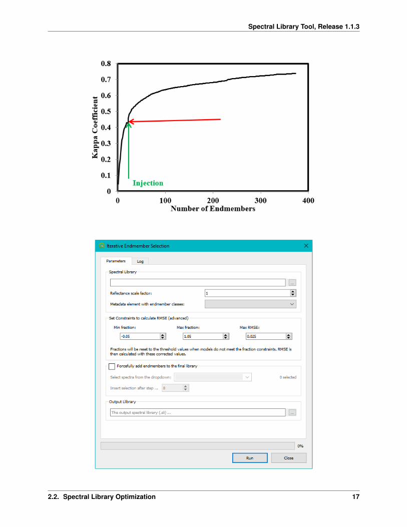
The Spectral Library Tool also includes a modified form of IES, called Forced IES, in which rare endmembers canbe identified in a library. Forced IES, which was originally proposed by Roth et al. [Roth2012], is needed when anendmember class is rare, but also important. Because it is rare, IES does not identify an endmember belonging to theclass if it results in a decrease in kappa. You can use another endmember selection tool, such as EMC, to identify thebest representative spectra from the rare class. One or more of these user-selected endmembers is then injected intothe endmember selection process after a set number of iterations, forcing IES to identify an optimal subset that alsoincludes the forced endmembers. As shown below, initially forcing the endmember results in a decrease in Kappa, butIES rapidly identifies models that increase accuracy, iterating until accuracy no longer improves. IES tends to generatemuch larger spectral libraries than EMC, but also results in higher classification accuracies.
IES was used by Roberts et al. ([Roberts2012]; [Roberts2017]) to discriminate urban surface materials, map plantspecies and estimate fractional cover in the Santa Barbara area, using MASTER to evaluate the relationship be-tween cover, species and land surface temperature ([Roberts2015]). Other applications of IES included creat-ing multi-temporal libraries for mapping vegetation species ([Dudley2015]) and improved mapping of fire severity([Fernandez2016]; [Quintano2017]). Roth et al. [Roth2015] evaluated the performance of IES across a diversity ofNorth American ecosystems, finding that Linear Discriminant Analysis (LDA) using Canonical Discriminant Analysis(CDA) was a superior classifier, but MESMA classification results could be improved using dimensionality reduction,such as CDA.
QGIS GUI
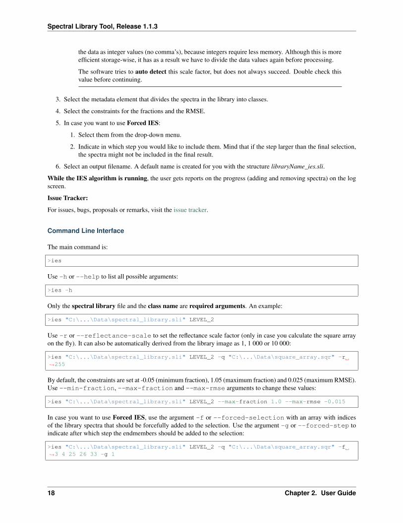
1. Select the input spectral library. Note that this library must have metadata attached to it and it is best sorted in away to assist interpretation of the square array.
2. The reflectance scale factor is automatically detected.
Note: Spectral data can be saved to file as reflectance values (i.e. values between 0 and 1) or thedata can be multiplied by a scale factor (usually by 1000 or 10000). This is done to be able to store
16 Chapter 2. User Guide
Spectral Library Tool, Release 1.1.3
2.2. Spectral Library Optimization 17
Spectral Library Tool, Release 1.1.3
the data as integer values (no comma’s), because integers require less memory. Although this is moreefficient storage-wise, it has as a result we have to divide the data values again before processing.
The software tries to auto detect this scale factor, but does not always succeed. Double check thisvalue before continuing.
3. Select the metadata element that divides the spectra in the library into classes.
4. Select the constraints for the fractions and the RMSE.
5. In case you want to use Forced IES:
1. Select them from the drop-down menu.
2. Indicate in which step you would like to include them. Mind that if the step larger than the final selection,the spectra might not be included in the final result.
6. Select an output filename. A default name is created for you with the structure libraryName_ies.sli.
While the IES algorithm is running, the user gets reports on the progress (adding and removing spectra) on the logscreen.
Issue Tracker:
For issues, bugs, proposals or remarks, visit the issue tracker.
Command Line Interface
The main command is:
>ies
Use -h or --help to list all possible arguments:
>ies -h
Only the spectral library file and the class name are required arguments. An example:
>ies "C:\...\Data\spectral_library.sli" LEVEL_2
Use -r or --reflectance-scale to set the reflectance scale factor (only in case you calculate the square arrayon the fly). It can also be automatically derived from the library image as 1, 1 000 or 10 000:
>ies "C:\...\Data\spectral_library.sli" LEVEL_2 -q "C:\...\Data\square_array.sqr" -r→˓255
By default, the constraints are set at -0.05 (minimum fraction), 1.05 (maximum fraction) and 0.025 (maximum RMSE).Use --min-fraction, --max-fraction and --max-rmse arguments to change these values:
>ies "C:\...\Data\spectral_library.sli" LEVEL_2 --max-fraction 1.0 --max-rmse -0.015
In case you want to use Forced IES, use the argument -f or --forced-selection with an array with indicesof the library spectra that should be forcefully added to the selection. Use the argument -g or --forced-step toindicate after which step the endmembers should be added to the selection:
>ies "C:\...\Data\spectral_library.sli" LEVEL_2 -q "C:\...\Data\square_array.sqr" -f→˓3 4 25 26 33 -g 1
18 Chapter 2. User Guide
Spectral Library Tool, Release 1.1.3
By default, the output file is stored in the same folder as the input file, with the extension ‘_ies.sli’. To select anotherfile or another location, use the argument -o or --output:
>ies "C:\...\Data\spectral_library.sli" LEVEL_2 -q "C:\...\Data\square_array.sqr" -o→˓"C:\...\Data\ies_library.sli"
Issue Tracker:
For issues, bugs, proposals or remarks, visit the issue tracker.
2.2.4 Constrained Reference Endmember Selection (CRES)
The CRES module represents an alternative approach to endmember selection. With CRES a user supplies expertknowledge on the expected SMA fractions at a particular location in order to select the optimal endmembers forthat site. This approach was first described by Roberts et al. [Roberts1993] and later discussed in more detail inRoberts et al. [Roberts1998]. It has been used extensively in a number of papers published out of the VIPER group toselect optimum endmembers for simple spectral mixture analysis ([Roberts2002], [Roberts2004]). CRES is a tool thataids the user to see which endmembers will produce SMA fractions that produce the closest match to the estimatedfractions.
QGIS GUI
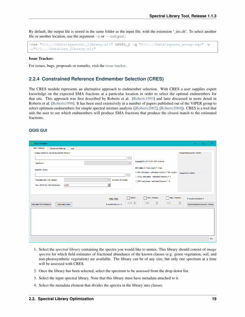
1. Select the spectral library containing the spectra you would like to unmix. This library should consist of imagespectra for which field estimates of fractional abundance of the known classes (e.g. green vegetation, soil, andnon-photosynthetic vegetation) are available. The library can be of any size, but only one spectrum at a timewill be assessed with CRES.
2. Once the library has been selected, select the spectrum to be assessed from the drop down list.
3. Select the input spectral library. Note that this library must have metadata attached to it.
4. Select the metadata element that divides the spectra in the library into classes.
2.2. Spectral Library Optimization 19
Spectral Library Tool, Release 1.1.3
5. The reflectance scale factor is automatically detected, but can be changed on the Advanced tab.
6. Select the unmixing RMSE constraint.
7. On the advanced tab, it is possible to include non-photometric shade.
8. To calculate SMA fractions and RMSE, click Calculate SMA fractions. Do this step only once.
Note: The table will now be filled with the SMA results (fractions and RMSE) for all models that meet theRMSE constraint. Models are identified by the spectra names.
9. Enter estimates of the endmember fraction under the label Target fractions for INDEX.
These estimated fractions may come from field data, expert knowledge or from some other ancillary data. Thesevalues are a critical component of CRES, as the main goal is to find the spectra that produce the closest fit tothese endmember fraction estimates. Depending on the quality of your initial estimates, you are likely to adjustthe fractions.
10. Enter weights for the indices calculations.
Example for the GV-index in a GV-SOIL-NPV mixture:
GV index = RMSE weight * RMSE+ |GV calculated - estimated fraction| * GV weight+ |SOIL calculated - estimated fraction|+ |NPV calculated - estimated fraction|+ |Shade calculated - estimated fraction|
Some experimentation is needed to assess the best weighting factors. Increasing the endmember weight placesthe greater importance on matching the fraction of the target endmember. Increasing the RMSE constraint placesgreater importance on the fit of the model, or the spectral shape.
Note: Because RMSE values (e.g., 0.025) are generally small relative to endmember fraction values (e.g., 0.3)an RMSE weight of 5 to 10 is generally helpful in ensuring that RMSE (model fit) is sufficiently weighted.
Note: Extra index columns are now added to the table. Play around by changing the index weight values andre-calculating the index. Smaller index numbers indicate better models.
The columns can be sorted by clicking on the headers.
11. Based on the results, the user can now select good spectra and export them as a new library.
Issue Tracker:
For issues, bugs, proposals or remarks, visit the issue tracker.
Command Line Interface
Because of the interactive nature of the CRES algorithm, no CLI is foreseen.
Issue Tracker:
For issues, bugs, proposals or remarks, visit the issue tracker.
20 Chapter 2. User Guide
Spectral Library Tool, Release 1.1.3
2.2.5 MUSIC
Unlike IES, MUSIC by [Iordache2014] is an image-based library pruning method designed to select, from a largelibrary, a subset of pure spectra that best represents the spectral variability of a given hyperspectral image and that, asa consequence, constitutes the best input for subpixel fractional abundance estimation.
MUSIC essentially comprises two steps. Firstly, the hyperspectral image is represented as a small set of eigenvectorsthat together define the image subspace, the n-dimensional space in which the data “live”. This step is accomplishedusing the HySime algorithm ([BioucasDias2008]), which needs no input parameters and estimates the required numberof eigenvectors (k) based on the signal- and noise correlation matrices of the original image.
Secondly, the Euclidean distances between each library spectrum and the estimated image subspace are calculatedthrough orthogonal projection. The resulting projection errors, or distances between library members and image, aresorted and the spectra corresponding to the lowest distances are selected. The number of spectra to be retained canbe adjusted by the user. In the complete absence of noise, the image is theoretically composed of k endmembers (asestimated by HySime). In practice however, this parameter is often set to 2 x k ([Iordache2014]).
In the current implementation, the user can set a minimum value for the number of eigenvectors to retain from theHySime algorithm.
MUSIC has already been successfully applied on both simulated and real hyperspectral datasets of mainly semi-naturalenvironments (i.e., citrus orchards) and has been shown to increase the accuracy and computational efficiency ofsubpixel fraction mapping using sparse unmixing ([Iordache2014]). However, [Degerickx2016] showed that in morecomplex, urban environments MUSIC has some remaining redundancies in the final spectral libraries and revealedpotential room for improvement.
MUSIC GUI
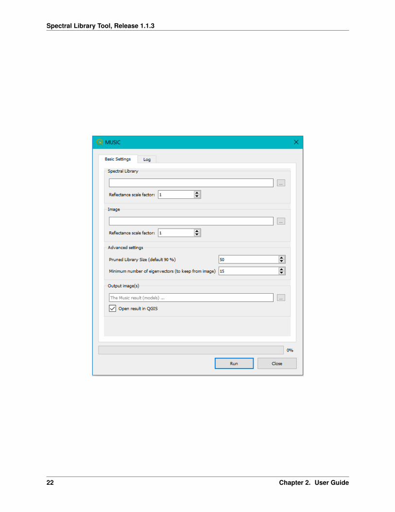
1. Select the input spectral library.
2. The reflectance scale factor is automatically detected.
Note: Spectral data can be saved to file as reflectance values (i.e. values between 0 and 1) or thedata can be multiplied by a scale factor (usually by 1000 or 10000). This is done to be able to storethe data as integer values (no comma’s), because integers require less memory. Although this is moreefficient storage-wise, it has as a result we have to divide the data values again before processing.
The software tries to auto detect this scale factor, but does not always succeed. Double check thisvalue before continuing.
3. Select the input image. Again the reflectance scale factor is automatically detected. Double check it.
4. Advanced settings:
• The size of the pruned library for MUSIC
• The minimum number of eigenvectors to be retained from the image to calculate MUSIC distances
5. Select an output filename. A default name is created for you with the structure libraryName_music.sli.
Issue Tracker:
For issues, bugs, proposals or remarks, visit the issue tracker.
2.2. Spectral Library Optimization 21
Spectral Library Tool, Release 1.1.3
22 Chapter 2. User Guide

Spectral Library Tool, Release 1.1.3
2.2.6 AMUSES
AMUSES (Automated MUsic and spectral Separability based Endmember Selection technique) by [Degerickx2017]is an extension on MUSIC. It adds a spectral separability measure to further decrease the internal redundancy withinthe library subset produced by MUSIC.
[Degerickx2016] combined MUSIC and IES and showed that this approach results in smaller spectral libraries, in turnyielding more robust results.
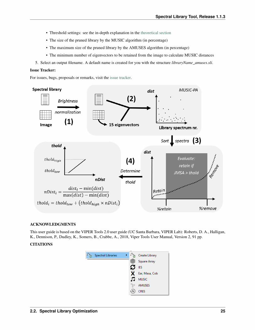
In AMUSES, [Degerickx2017] opted for a spectral separability metric instead of IES to have more control over theentire procedure. A schematic overview of AMUSES is provided in the image below.
The method starts by applying brightness normalization to both the original spectral library and the image, to decreasethe effect of brightness during the endmember selection process (step 1 in the figure below). This is accomplished bydividing the reflectance in each band by the average reflectance of the entire signal [Wu2004].
Then MUSIC is used to calculate the distance from each library spectrum to the image (step 2 in the figure below).[Degerickx2017] used a fixed minimum number of eigenvectors (15).The more eigenvectors are retained, the morespectra will be ranked as highly similar to the image and the harder it becomes to identify the true image endmembers.
After ranking all library spectra according to their distance to the image, a fraction of spectra ranked highest areretained and the lowest few are discarded (step 3 in the figure below).
All remaining spectra are assessed one by one using a spectral separability measure: only if a signature is sufficientlydissimilar from the already selected spectra, it will be included in the final selection.
[Degerickx2017] used a metric that combines the Jeffries Matusita distance and Spectral Angle (JMSA) by[Padma2014].
The JMSA threshold is systematically increased. This threshold is used to evaluate the similarity of a candidatespectrum with the already selected spectra (thold parameter in the figure below) in function of the normalized distanceof the candidate spectrum to the image as calculated by MUSIC (*nDist in the figure below).
The higher the MUSIC distance, the lower the relevance of a library member to the image being analyzed. By usinga high JMSA threshold for these spectra, their chance of ending up in the final selection is decreased. As input to thealgorithm, the user needs to define a minimum and maximum threshold between which the thold parameter is allowedto vary.
Using this approach, the pruning algorithm is highly automated as it now decides on the final number of spectra to beretained based on the distance to the image and the mutual similarity of the library spectra.
AMUSES GUI
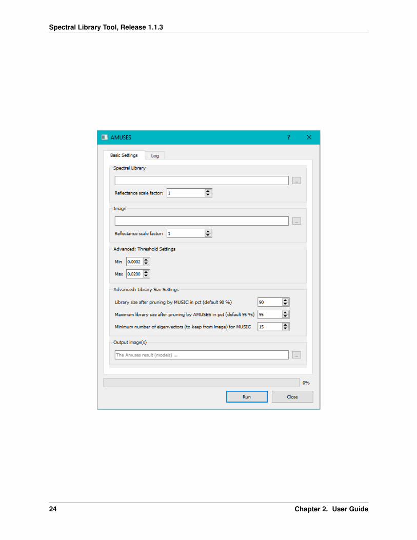
1. Select the input spectral library.
2. The reflectance scale factor is automatically detected.
Note: Spectral data can be saved to file as reflectance values (i.e. values between 0 and 1) or thedata can be multiplied by a scale factor (usually by 1000 or 10000). This is done to be able to storethe data as integer values (no comma’s), because integers require less memory. Although this is moreefficient storage-wise, it has as a result we have to divide the data values again before processing.
The software tries to auto detect this scale factor, but does not always succeed. Double check thisvalue before continuing.
3. Select the input image. Again the reflectance scale factor is automatically detected. Double check it.
4. Advanced settings:
2.2. Spectral Library Optimization 23
Spectral Library Tool, Release 1.1.3
24 Chapter 2. User Guide
Spectral Library Tool, Release 1.1.3
• Threshold settings: see the in-depth explanation in the theoretical section
• The size of the pruned library by the MUSIC algorithm (in percentage)
• The maximum size of the pruned library by the AMUSES algorithm (in percentage)
• The minimum number of eigenvectors to be retained from the image to calculate MUSIC distances
5. Select an output filename. A default name is created for you with the structure libraryName_amuses.sli.
Issue Tracker:
For issues, bugs, proposals or remarks, visit the issue tracker.
ACKNOWLEDGMENTS
This user guide is based on the VIPER Tools 2.0 user guide (UC Santa Barbara, VIPER Lab): Roberts, D. A., Halligan,K., Dennison, P., Dudley, K., Somers, B., Crabbe, A., 2018, Viper Tools User Manual, Version 2, 91 pp.
CITATIONS
2.2. Spectral Library Optimization 25

Spectral Library Tool, Release 1.1.3
26 Chapter 2. User Guide

CHAPTER 3
Exercises
For issues, bugs, proposals or remarks, visit the issue tracker.
We have developed two exercises. One with a data set in Brussels (Belgium), and one with a data set in Santa Barbara,CA (USA).
These exercises consist of two parts: creating and optimizing spectral libraries and MESMA and post-processing: theformer you find here; for the latter visit http://mesma.readthedocs.io.
3.1 Exercise Brussels
For issues, bugs, proposals or remarks, visit the issue tracker.
3.1.1 Objectives
1. Learn to work with the Spectral Library Tool in QGIS
2. Get familiarized with spectral libraries:
• Build and edit them
• Prune libraries with optimization techniques like EMC or IES
• Analyse them with the Library Viewer
3. Use MESMA as a sub-pixel classification method
Part 2 on http://mesma.readthedocs.be.
3.1.2 Tutorial Data Set
You can download the tutorial data set tutorial_data_set_brussels from https://bitbucket.org/kul-reseco/spectral-libraries/downloads/. The zip file contains the following data:
27
Spectral Library Tool, Release 1.1.3
• Apex images from 2015 with numbers 014, 14 and 180 in ENVI format
• A spectral library in ENVI format
• A validation shape file for each image
• Note: images and library have been smoothed using Savitzky-Golay filter with window size 9
Acknowledgement for the data set:
Degerickx, Roberts, Somers; 2019; Enhancing the performance of Multiple Endmember Spectral Mixture Analysis(MESMA) for urban land cover mapping using airborne lidar data and band selection; Volume 221; P 260-273
Note: It is good practice to keep all files in the same folder - especially during the exercises. Files like square arraysoften go looking for library information on which they are built.
3.1.3 Image Inspection
1. Try to visualize the images in QGIS.
To recognize the surroundings, overlay them with a map from the OpenStreetMap project (QuickMapSer-vices plugin and Google Satellite View).
2. Inspect the technical properties of the image.
• Why are the images black when first loading them into QGIS? Which bands would you use to visualize themfor easy interpretation? Look-up the wavelengths of the RGB bands.
• What is the size of the image and of each pixel?
• Make a list of the land cover classes you expect to find in each image.
3.1.4 Creating Spectral Libraries
You will find some Spectral Libraries in your data folder. We will not use them for now. In this exercise, you aresupposed to create your own Spectral Library by selecting pure pixels from your image.
Exercise: Create a Spectral Library
Data
Use the image apex_2015_180_smooth.
Exercise
For each land cover class (see previous exercise), try to find several good spectra to add to the Spectral Library. Don’tforget to add a metadata class for each spectrum. You won’t remember afterwards!
• Turn off the OpenStreetMap layer in order not to get errors.
• Zoom to one of the images.
• Open the tool to build your own Spectral Library .
• Click on some random pixels and see the features appear on the plotting window. Add them to your spectrallibrary by clicking on the Add button .
28 Chapter 3. Exercises
Spectral Library Tool, Release 1.1.3
• Toggle the Auto button to automatically add profile to your spectral library.
• To remove a profile, select it in the attribute table and use the Delete button .
• You can now edit the profile metadata, add or remove non-compulsory fields and zoom/pan to selection on theimage.
• Save the Spectral Library to the ENVI Spectral Library format (.sli) .
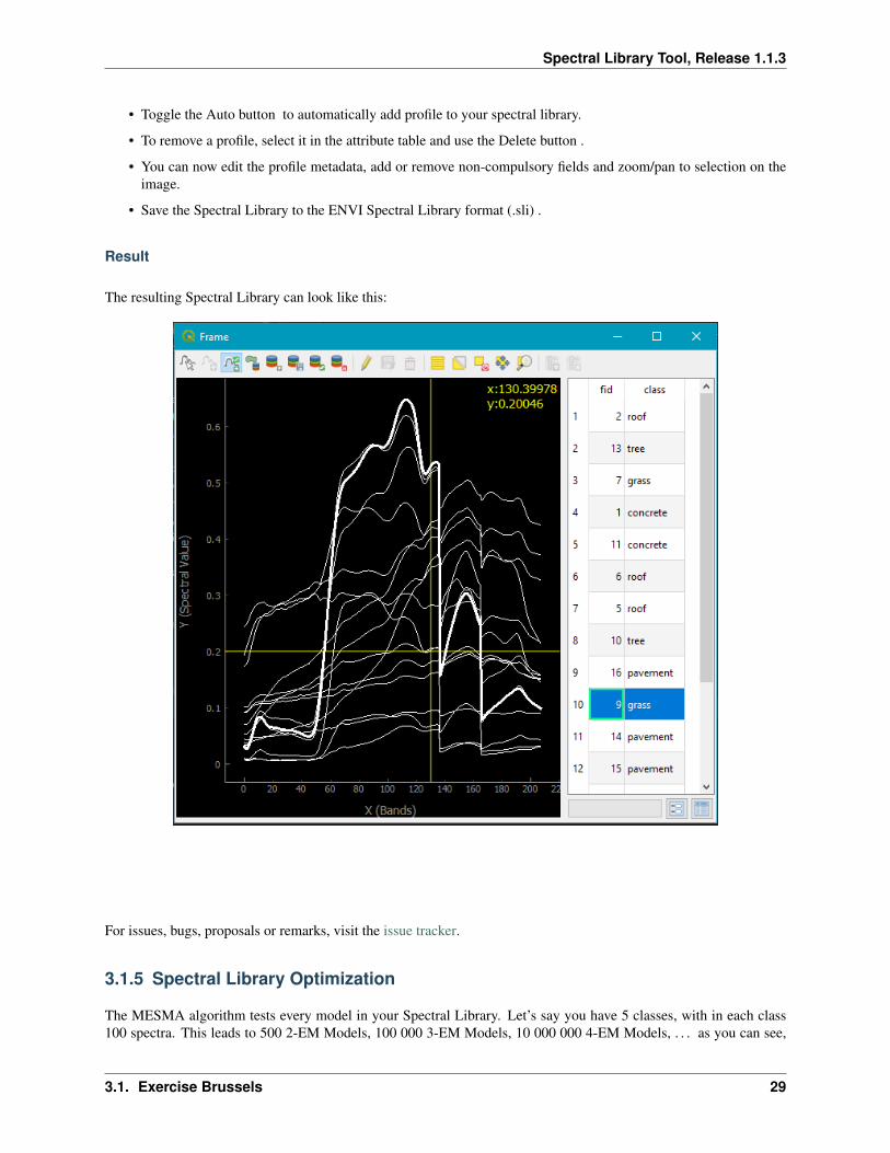
Result
The resulting Spectral Library can look like this:
For issues, bugs, proposals or remarks, visit the issue tracker.
3.1.5 Spectral Library Optimization
The MESMA algorithm tests every model in your Spectral Library. Let’s say you have 5 classes, with in each class100 spectra. This leads to 500 2-EM Models, 100 000 3-EM Models, 10 000 000 4-EM Models, . . . as you can see,
3.1. Exercise Brussels 29
Spectral Library Tool, Release 1.1.3
this can quickly get out of hand. Therefore it is good practice to prune your library, i.e. reduce it by removing spectrathat are very similar.
In this exercise, we determine which spectra within a given class (e.g. Soil or Trees) are most representative of theirclass, while covering the range of variability within the class.
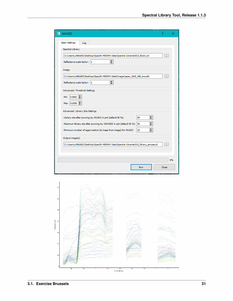
Exercise: Run AMUSES
Data used
We will use the Spectral Library (library.sli) from the testdata. To analyse this library first, use the spectral library tool. In this tool, use the Open Library button and browse to this file.
How many spectra does this library contain?
What are the different classes and subclasses in this library and how many are there?
To help you interpret the different classes, have a look at table 2 in the paper of Jeroen Degerickx (find it in yourexercise folder):
Degerickx, Roberts, Somers; 2019; Enhancing the performance of Multiple Endmember Spectral Mixture Analysis(MESMA) for urban land cover mapping using airborne lidar data and band selection; Volume 221; P 260-273
We will also be using the image apex_2015_180_smooth. This is a hyperspectral Apex image from 2015 in ENVIformat.
Exercise
Spectral Library:
• Select library.sli.
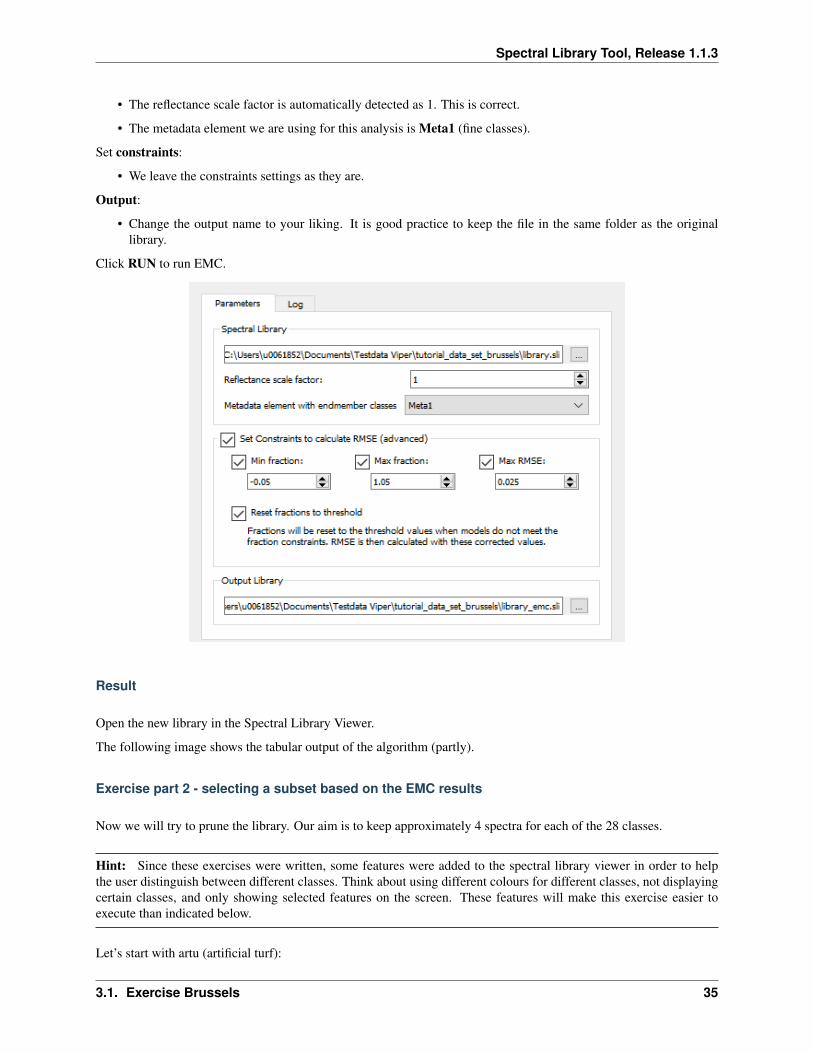
• The reflectance scale factor is automatically detected as 1. This is correct.
Image:
• Select apex_2015_180_smooth.
• The reflectance scale factor is automatically detected as 1. This is correct.
Advanced Settings:
• We will leave all settings as they are.
Output:
• The default output name is library_amuses.sli.
Click RUN to run AMUSES. The progress should be shown on the log-tab.
Result
The final library consists of 71 spectra.
For issues, bugs, proposals or remarks, visit the issue tracker.
30 Chapter 3. Exercises
Spectral Library Tool, Release 1.1.3
3.1. Exercise Brussels 31
Spectral Library Tool, Release 1.1.3
Exercise: Run IES
Data used
We will use the Spectral Library (library.sli) from the testdata. To analyse this library first, use the spectral library tool. In this tool, use the Open Library button and browse to this file.
How many spectra does this library contain?
What are the different classes and subclasses in this library and how many are there?
To help you interpret the different classes, have a look at table 2 in the paper of Jeroen Degerickx (find it in yourexercise folder):
Degerickx, Roberts, Somers; 2019; Enhancing the performance of Multiple Endmember Spectral Mixture Analysis(MESMA) for urban land cover mapping using airborne lidar data and band selection; Volume 221; P 260-273
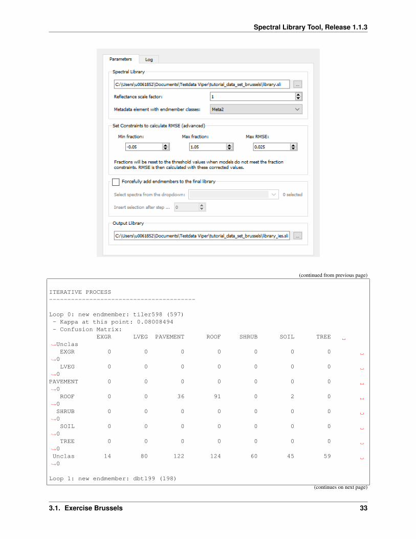
Exercise
Spectral Library:
• Select library.sli.
• The reflectance scale factor is automatically detected as 1. This is correct.
• The metadata element we are using for this analysis is Meta2.
Set constraints:
• We leave the constraints settings as they are.
Forced IES:
• We will not use this option in this exercise.
Output:
• The default output name is library_ies.sli.
Click RUN to run IES. The progress should be shown on the log-tab. But since this is a very heavy process, QGISmight freeze for the duration of the process. IES is quite slow and might take a while.
Result
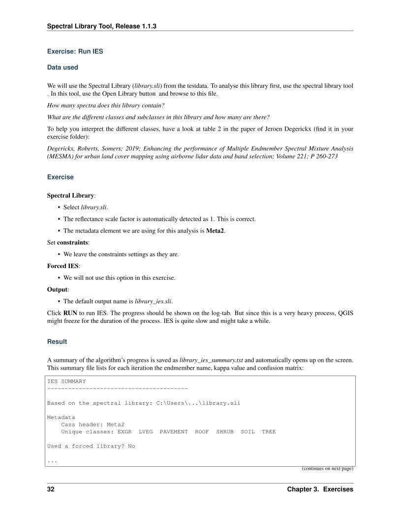
A summary of the algorithm’s progress is saved as library_ies_summary.txt and automatically opens up on the screen.This summary file lists for each iteration the endmember name, kappa value and confusion matrix:
IES SUMMARY----------------------------------------
Based on the spectral library: C:\Users\...\library.sli
MetadataCass header: Meta2Unique classes: EXGR LVEG PAVEMENT ROOF SHRUB SOIL TREE
Used a forced library? No
...
(continues on next page)
32 Chapter 3. Exercises
Spectral Library Tool, Release 1.1.3
(continued from previous page)
ITERATIVE PROCESS----------------------------------------
Loop 0: new endmember: tiler598 (597)- Kappa at this point: 0.08008494- Confusion Matrix:
EXGR LVEG PAVEMENT ROOF SHRUB SOIL TREE→˓Unclas
EXGR 0 0 0 0 0 0 0→˓0
LVEG 0 0 0 0 0 0 0→˓0PAVEMENT 0 0 0 0 0 0 0→˓0
ROOF 0 0 36 91 0 2 0→˓0SHRUB 0 0 0 0 0 0 0
→˓0SOIL 0 0 0 0 0 0 0
→˓0TREE 0 0 0 0 0 0 0
→˓0Unclas 14 80 122 124 60 45 59→˓0
Loop 1: new endmember: dbt199 (198)
(continues on next page)
3.1. Exercise Brussels 33
Spectral Library Tool, Release 1.1.3
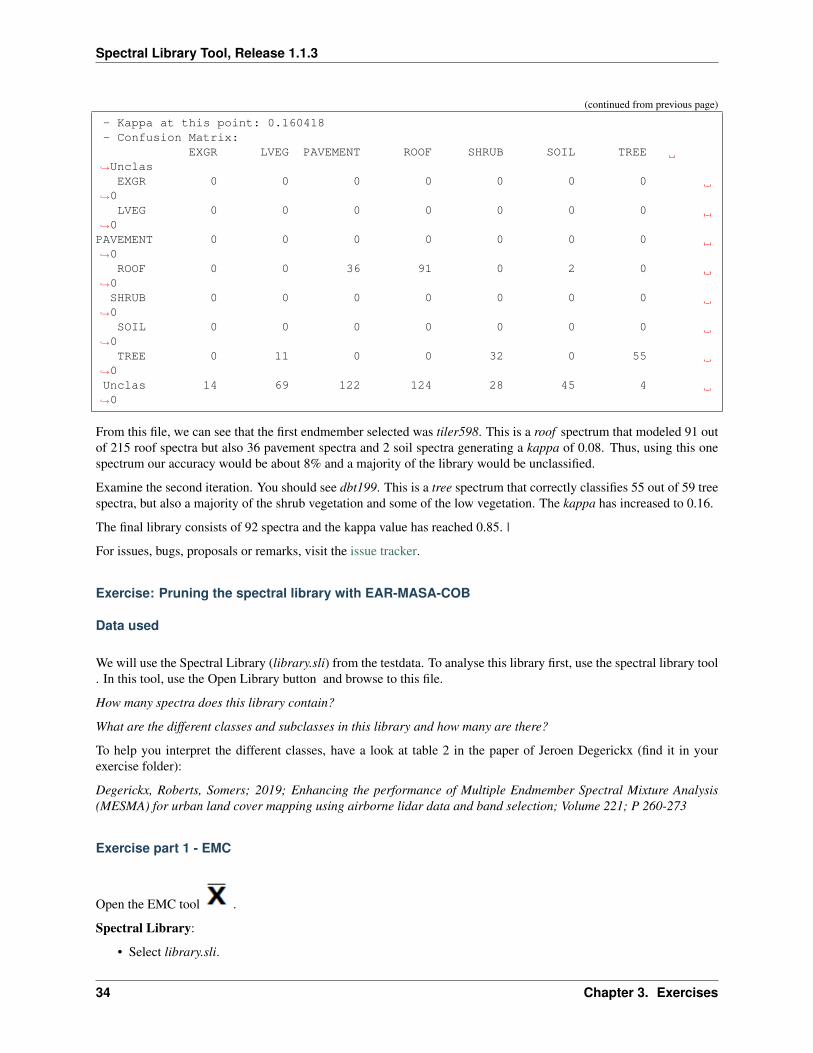
(continued from previous page)
- Kappa at this point: 0.160418- Confusion Matrix:
EXGR LVEG PAVEMENT ROOF SHRUB SOIL TREE→˓Unclas
EXGR 0 0 0 0 0 0 0→˓0
LVEG 0 0 0 0 0 0 0→˓0PAVEMENT 0 0 0 0 0 0 0→˓0
ROOF 0 0 36 91 0 2 0→˓0SHRUB 0 0 0 0 0 0 0
→˓0SOIL 0 0 0 0 0 0 0
→˓0TREE 0 11 0 0 32 0 55
→˓0Unclas 14 69 122 124 28 45 4→˓0
From this file, we can see that the first endmember selected was tiler598. This is a roof spectrum that modeled 91 outof 215 roof spectra but also 36 pavement spectra and 2 soil spectra generating a kappa of 0.08. Thus, using this onespectrum our accuracy would be about 8% and a majority of the library would be unclassified.
Examine the second iteration. You should see dbt199. This is a tree spectrum that correctly classifies 55 out of 59 treespectra, but also a majority of the shrub vegetation and some of the low vegetation. The kappa has increased to 0.16.
The final library consists of 92 spectra and the kappa value has reached 0.85. |
For issues, bugs, proposals or remarks, visit the issue tracker.
Exercise: Pruning the spectral library with EAR-MASA-COB
Data used
We will use the Spectral Library (library.sli) from the testdata. To analyse this library first, use the spectral library tool. In this tool, use the Open Library button and browse to this file.
How many spectra does this library contain?
What are the different classes and subclasses in this library and how many are there?
To help you interpret the different classes, have a look at table 2 in the paper of Jeroen Degerickx (find it in yourexercise folder):
Degerickx, Roberts, Somers; 2019; Enhancing the performance of Multiple Endmember Spectral Mixture Analysis(MESMA) for urban land cover mapping using airborne lidar data and band selection; Volume 221; P 260-273
Exercise part 1 - EMC
Open the EMC tool .
Spectral Library:
• Select library.sli.
34 Chapter 3. Exercises
Spectral Library Tool, Release 1.1.3
• The reflectance scale factor is automatically detected as 1. This is correct.
• The metadata element we are using for this analysis is Meta1 (fine classes).
Set constraints:
• We leave the constraints settings as they are.
Output:
• Change the output name to your liking. It is good practice to keep the file in the same folder as the originallibrary.
Click RUN to run EMC.
Result
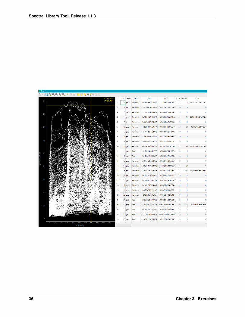
Open the new library in the Spectral Library Viewer.
The following image shows the tabular output of the algorithm (partly).
Exercise part 2 - selecting a subset based on the EMC results
Now we will try to prune the library. Our aim is to keep approximately 4 spectra for each of the 28 classes.
Hint: Since these exercises were written, some features were added to the spectral library viewer in order to helpthe user distinguish between different classes. Think about using different colours for different classes, not displayingcertain classes, and only showing selected features on the screen. These features will make this exercise easier toexecute than indicated below.
Let’s start with artu (artificial turf):
3.1. Exercise Brussels 35
Spectral Library Tool, Release 1.1.3
36 Chapter 3. Exercises
Spectral Library Tool, Release 1.1.3
• The class has originally 22 spectra.
• We see that artu16 was successful in modelling all other spectra in the class (InCOB of 21).
• The EAR values range between 0.009 and 0.031. artu16 has an EAR value of 0.014, not the lowest but quitelow. The lowest EAR values are for artu12, artu13, artu15, artu2, artu1 and artu10.
• The MASA values range between 0.090 and 0.210. artu16 has the highest MASA value! The lowest MASAvalues are for artu1, artu22, artu11, artu18, artu17, artu13 and artu21.
• The only similarities are artu13 and artu1.
How do we explain this?
• Remove all other spectra except for the artu class. Don’t worry, this action does not affect the library saved onfile.
• You can see that there are a lot of similar, dark spectra and a few very distinct bright ones.
• artu1 lies in the group of similar spectra, explaining the good MASA value.
• artu12 lies somewhere in the middle of everything, with a form similar to the dark spectra, explaining the goodEAR value.
• artu16 is the brightest one with a very different shape – think about why this one would be selected.
We keep those three spectra.
Then we go on with dbt (deciduous broad leaf trees):
• Reload the full library and now remove all spectra except for the dbt class.
• This class contains 29 spectra.
• dbt199 was the only one able to model 27 other spectra (InCOB value of 27). Again this is the most brightspectrum in the class. Does this ring any bell?
• dbt199 also has the best EAR value.
• If you look at the top 5 of MASA values, you see that 4 of them are also in the top 5 of EAR values and viceversa: dbt199, dbt176, dbt189 and dbt198.
• Looking at dbt189 and dbt198 we see that they are (almost) identical.
• We keep the top 3.
Why are EAR and InCOB results so similar, but MASA less?
Go on and select the 3 or 4 best spectra for each class. You can skip the classes Extensive Green Roof, Meadow, RedGravel, Green Surface, Tartan, Bare Soil and Sand. They are not part of our images.
For issues, bugs, proposals or remarks, visit the issue tracker.
Click on these links to find the theory behind AMUSES, IES and EMC.
For issues, bugs, proposals or remarks, visit the issue tracker.
3.2 Exercise Santa Barbara
For issues, bugs, proposals or remarks, visit the issue tracker.
3.2. Exercise Santa Barbara 37
Spectral Library Tool, Release 1.1.3
3.2.1 Tutorial Data Set
You can download the tutorial data set tutorial_data_set_santa_barbara from https://bitbucket.org/kul-reseco/spectral-libraries/downloads/. The zip file contains the following data:
• Image 010614r4_4-5_clip
A 2001 AVIRIS image (ENVI header format) with 20 m spatial resolution ([Roberts2003]).
• Image demo1.sub
A 2011 AVIRIS image (ENVI header format) as 600x600 pixel subset of downtown Santa Barbara([Roberts2015], [Roberts2017]. AVIRIS data were processed to apparent surface reflectance usingATCOR, as described in [Roberts2015], and scaled to reflectance times 10,000.
• Spectral Library: roberts2017_urban.sli
This library was used in [Roberts2017] and consists of 3725 spectra. The spectra include a mixtureof spectra extracted from the three AVIRIS flight lines acquired in 2011 merged with the urbanspectral library described by [Herold2004]. The AVIRIS spectra, which originally consisted of over60,000 spectra, were subsampled using code developed by Keely Roth as part of her dissertation.Following the protocols described in [Roth2012], spectra were sampled at the polygon level suchthat no polygon can contribute more than 10 spectra to the library, or more than 50% of the pixelsfor small polygons. The p9 in the file name, implies this was the 9th random pull out of 10 pulls.The 9th pull was selected because it produced the highest accuracy (based on IES) with the lowestnumber of spectra, as described in [Roberts2017].
• Spectral Library: 010627_westusa_all.sli
Spectral Library for the CRES tutorial and for Simple SMA.
• Spectral Library: roberts_et_al_2017_final.sli.
This is the same library that was used to generate the final fraction maps in Roberts et al. (2017). Thelibrary was created by merging 2,739 spectra extracted from the image with 986 spectra measuredin the field. IES was run, generating a 497 spectral subset. This library was further pruned toremove poorly performing models to generate a 376 endmember subset, then all clearly mixed spectra(assessed visually), were removed to generate the nomix library, consisting of 259 spectra. Finally, aprocedure, designed to remove spectrally degenerate spectra was used to generate a 91 endmembersubset. The final culling was accomplished in 8 iterations.
• roi.shp
This contains regions of interest for most dominant cover types in the region. This matchesdemo1.sub.
Acknowledgement for the data set:
Roberts, D. A., Halligan, K., Dennison, P., Dudley, K., Somers, B., Crabbe, A., 2018, Viper Tools User Manual, Version2, 91 pp.
Note: It is good practice to keep all files in the same folder - especially during the exercises. Files like square arraysoften go looking for library information on which they are built.
3.2.2 Creating Spectral Libraries
38 Chapter 3. Exercises
Spectral Library Tool, Release 1.1.3
Exercise: Create a Spectral Library
Objective: In this exercise, we will build a Spectral Library, based on an image and it’s ROI’s (Regions Of Interest).
Data used
• Image: demo1.sub
To display the image as true color image, use RGB wavelengths 0.658, 0.560 and 0.443 𝜇m.
• Regions Of Interest: roi.shp
You might notice a lot of polygons in the ROI layer lie outside the image. This is no problem. Analyze the metadata:each ROI should have associated metadata like impervious/pervious, vegetation type, etc. The features represent amix of natural and anthropogenic materials from needle-leaf shrubs (ADFA) and the invasive plant species Brassicanigra (BRNI), to asphalt surfaces, red tile roofs, concrete and golf courses. The metadata headers are generic becausethere is no hierarchical level common to a plant, a soil or an impervious surface (what is the species of asphalt, or itslife form?).
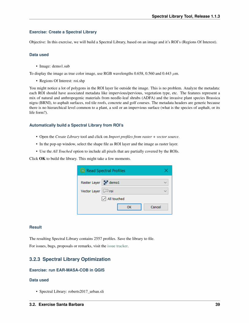
Automatically build a Spectral Library from ROI’s
• Open the Create Library tool and click on Import profiles from raster + vector source.
• In the pop-up window, select the shape file as ROI layer and the image as raster layer.
• Use the All Touched option to include all pixels that are partially covered by the ROIs.
Click OK to build the library. This might take a few moments.
Result
The resulting Spectral Library contains 2557 profiles. Save the library to file.
For issues, bugs, proposals or remarks, visit the issue tracker.
3.2.3 Spectral Library Optimization
Exercise: run EAR-MASA-COB in QGIS
Data used
• Spectral Library: roberts2017_urban.sli
3.2. Exercise Santa Barbara 39
Spectral Library Tool, Release 1.1.3
Part 1 - EMC
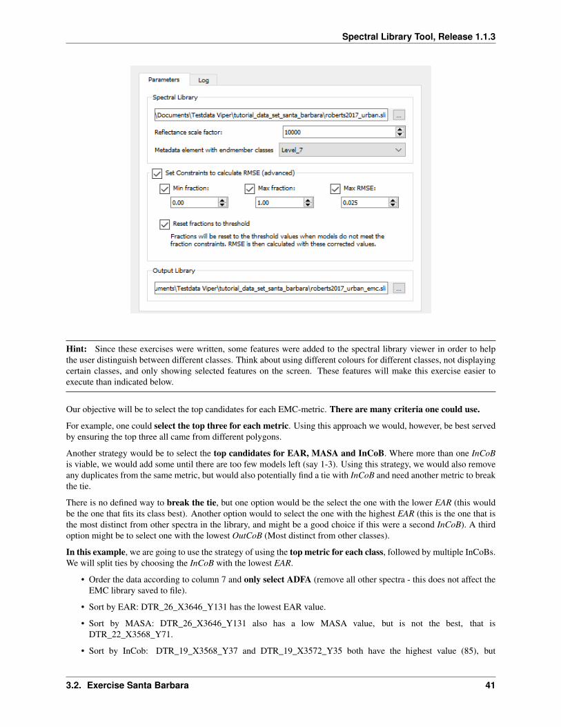
Select the input spectral library.
• Select roberts2017_urban.sli.
• The reflectance scale factor is automatically detected as 10000. This is correct.
• The metadata element we are using for this analysis is Level_7.
Set constraints:
• Minimum fraction to 0.0, maximum to 1.0 and RMSE constraint at 0.025.
• Select the ‘Reset fractions to threshold’ mode.
Output:
• Select a name for the new library, e.g. roberts2017_urban_emc.sli.
Click OK to run EMC.
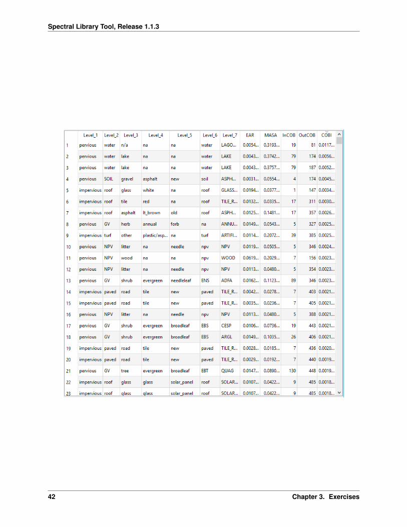
Result
The following image shows the tabular output of the algorithm (partly).
• When the metric of choice is Cob, sorting works very well.
The best candidate per Level_7 class is the class with the highest InCob value. In case of a tie, look to othermeasures (such as EAR) to make your choice.
• When the metric of choice is EAR or MASA, this technique is less efficient, as there are many similar RMSE orspectral angles values.
Part 2 - selecting a subset based on the EMC results
40 Chapter 3. Exercises
Spectral Library Tool, Release 1.1.3
Hint: Since these exercises were written, some features were added to the spectral library viewer in order to helpthe user distinguish between different classes. Think about using different colours for different classes, not displayingcertain classes, and only showing selected features on the screen. These features will make this exercise easier toexecute than indicated below.
Our objective will be to select the top candidates for each EMC-metric. There are many criteria one could use.
For example, one could select the top three for each metric. Using this approach we would, however, be best servedby ensuring the top three all came from different polygons.
Another strategy would be to select the top candidates for EAR, MASA and InCoB. Where more than one InCoBis viable, we would add some until there are too few models left (say 1-3). Using this strategy, we would also removeany duplicates from the same metric, but would also potentially find a tie with InCoB and need another metric to breakthe tie.
There is no defined way to break the tie, but one option would be the select the one with the lower EAR (this wouldbe the one that fits its class best). Another option would to select the one with the highest EAR (this is the one that isthe most distinct from other spectra in the library, and might be a good choice if this were a second InCoB). A thirdoption might be to select one with the lowest OutCoB (Most distinct from other classes).
In this example, we are going to use the strategy of using the top metric for each class, followed by multiple InCoBs.We will split ties by choosing the InCoB with the lowest EAR.
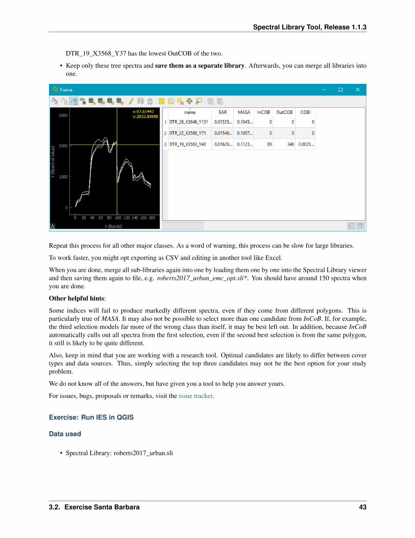
• Order the data according to column 7 and only select ADFA (remove all other spectra - this does not affect theEMC library saved to file).
• Sort by EAR: DTR_26_X3646_Y131 has the lowest EAR value.
• Sort by MASA: DTR_26_X3646_Y131 also has a low MASA value, but is not the best, that isDTR_22_X3568_Y71.
• Sort by InCob: DTR_19_X3568_Y37 and DTR_19_X3572_Y35 both have the highest value (85), but
3.2. Exercise Santa Barbara 41
Spectral Library Tool, Release 1.1.3
42 Chapter 3. Exercises
Spectral Library Tool, Release 1.1.3
DTR_19_X3568_Y37 has the lowest OutCOB of the two.
• Keep only these tree spectra and save them as a separate library. Afterwards, you can merge all libraries intoone.
Repeat this process for all other major classes. As a word of warning, this process can be slow for large libraries.
To work faster, you might opt exporting as CSV and editing in another tool like Excel.
When you are done, merge all sub-libraries again into one by loading them one by one into the Spectral Library viewerand then saving them again to file, e.g. roberts2017_urban_emc_opt.sli*. You should have around 150 spectra whenyou are done.
Other helpful hints:
Some indices will fail to produce markedly different spectra, even if they come from different polygons. This isparticularly true of MASA. It may also not be possible to select more than one candidate from InCoB. If, for example,the third selection models far more of the wrong class than itself, it may be best left out. In addition, because InCoBautomatically culls out all spectra from the first selection, even if the second best selection is from the same polygon,it still is likely to be quite different.
Also, keep in mind that you are working with a research tool. Optimal candidates are likely to differ between covertypes and data sources. Thus, simply selecting the top three candidates may not be the best option for your studyproblem.
We do not know all of the answers, but have given you a tool to help you answer yours.
For issues, bugs, proposals or remarks, visit the issue tracker.
Exercise: Run IES in QGIS
Data used
• Spectral Library: roberts2017_urban.sli
3.2. Exercise Santa Barbara 43

Spectral Library Tool, Release 1.1.3
Run IES
Select the input spectral library.
• Select roberts2017_urban.sli.
• The reflectance scale factor is automatically detected as 10000. This is correct.
• The metadata element we are using for this analysis is Level_7.
Set constraints:
• Minimum fraction to 0.0, maximum to 1.0 and RMSE constraint at 0.025.
Forced IES:
• We will not use this option in this exercise.
Output:
• The default output name is roberts2017_urban_ies.sli.
Click OK to run IES. The progress should be shown on the log-tab. But since this is a very heavy process, QGIS mightfreeze for the duration of the process. IES is quite slow and might take a while.
Result
A summary of the algorithm’s progress is saved as roberts2017_urban_ies_summary.txt. This summary file lists foreach iteration the endmember name, kappa value and confusion matrix:
44 Chapter 3. Exercises
Spectral Library Tool, Release 1.1.3
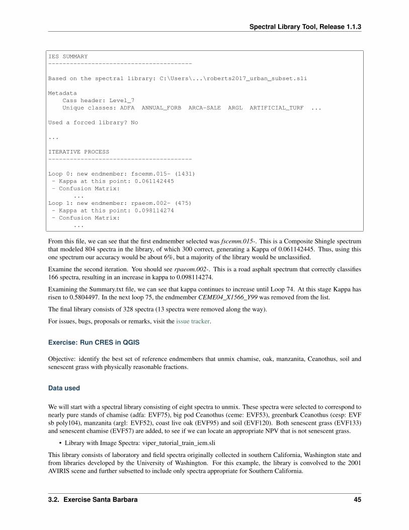
IES SUMMARY----------------------------------------
Based on the spectral library: C:\Users\...\roberts2017_urban_subset.sli
MetadataCass header: Level_7Unique classes: ADFA ANNUAL_FORB ARCA-SALE ARGL ARTIFICIAL_TURF ...
Used a forced library? No
...
ITERATIVE PROCESS----------------------------------------
Loop 0: new endmember: fscemm.015- (1431)- Kappa at this point: 0.061142445- Confusion Matrix:
...Loop 1: new endmember: rpaeom.002- (475)- Kappa at this point: 0.098114274- Confusion Matrix:
...
From this file, we can see that the first endmember selected was fscemm.015-. This is a Composite Shingle spectrumthat modeled 804 spectra in the library, of which 300 correct, generating a Kappa of 0.061142445. Thus, using thisone spectrum our accuracy would be about 6%, but a majority of the library would be unclassified.
Examine the second iteration. You should see rpaeom.002-. This is a road asphalt spectrum that correctly classifies166 spectra, resulting in an increase in kappa to 0.098114274.
Examining the Summary.txt file, we can see that kappa continues to increase until Loop 74. At this stage Kappa hasrisen to 0.5804497. In the next loop 75, the endmember CEME04_X1566_Y99 was removed from the list.
The final library consists of 328 spectra (13 spectra were removed along the way).
For issues, bugs, proposals or remarks, visit the issue tracker.
Exercise: Run CRES in QGIS
Objective: identify the best set of reference endmembers that unmix chamise, oak, manzanita, Ceanothus, soil andsenescent grass with physically reasonable fractions.
Data used
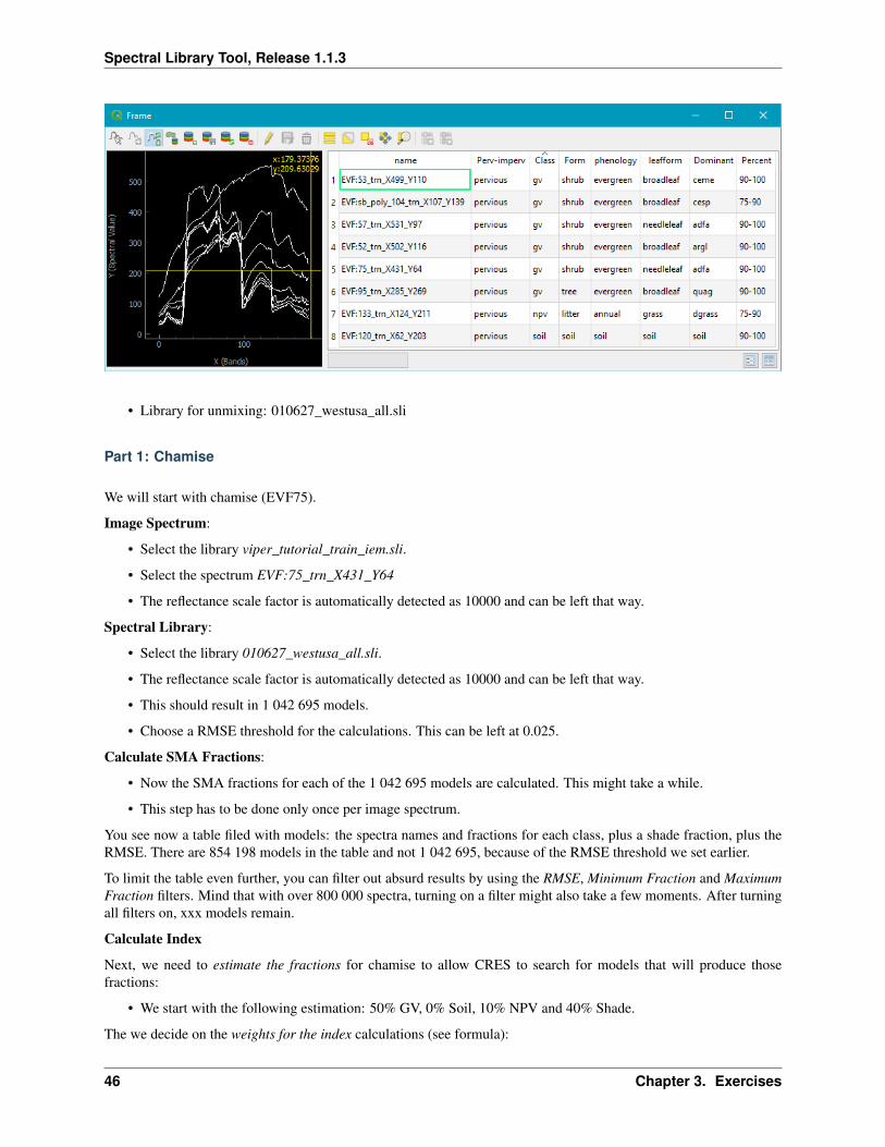
We will start with a spectral library consisting of eight spectra to unmix. These spectra were selected to correspond tonearly pure stands of chamise (adfa: EVF75), big pod Ceanothus (ceme: EVF53), greenbark Ceanothus (cesp: EVFsb poly104), manzanita (argl: EVF52), coast live oak (EVF95) and soil (EVF120). Both senescent grass (EVF133)and senescent chamise (EVF57) are added, to see if we can locate an appropriate NPV that is not senescent grass.
• Library with Image Spectra: viper_tutorial_train_iem.sli
This library consists of laboratory and field spectra originally collected in southern California, Washington state andfrom libraries developed by the University of Washington. For this example, the library is convolved to the 2001AVIRIS scene and further subsetted to include only spectra appropriate for Southern California.
3.2. Exercise Santa Barbara 45
Spectral Library Tool, Release 1.1.3
• Library for unmixing: 010627_westusa_all.sli
Part 1: Chamise
We will start with chamise (EVF75).
Image Spectrum:
• Select the library viper_tutorial_train_iem.sli.
• Select the spectrum EVF:75_trn_X431_Y64
• The reflectance scale factor is automatically detected as 10000 and can be left that way.
Spectral Library:
• Select the library 010627_westusa_all.sli.
• The reflectance scale factor is automatically detected as 10000 and can be left that way.
• This should result in 1 042 695 models.
• Choose a RMSE threshold for the calculations. This can be left at 0.025.
Calculate SMA Fractions:
• Now the SMA fractions for each of the 1 042 695 models are calculated. This might take a while.
• This step has to be done only once per image spectrum.
You see now a table filed with models: the spectra names and fractions for each class, plus a shade fraction, plus theRMSE. There are 854 198 models in the table and not 1 042 695, because of the RMSE threshold we set earlier.
To limit the table even further, you can filter out absurd results by using the RMSE, Minimum Fraction and MaximumFraction filters. Mind that with over 800 000 spectra, turning on a filter might also take a few moments. After turningall filters on, xxx models remain.
Calculate Index
Next, we need to estimate the fractions for chamise to allow CRES to search for models that will produce thosefractions:
• We start with the following estimation: 50% GV, 0% Soil, 10% NPV and 40% Shade.
The we decide on the weights for the index calculations (see formula):
46 Chapter 3. Exercises
Spectral Library Tool, Release 1.1.3
• Set the weights for the fractions to 1 and the RMSE to 10.
• Click Calculate Index.
• Sort by GV index.
Result for Chamise (adfa)
The best GV index (0.146) leads to a selections of CCEOLSTCK (52% GV, -1% Soil, 9% NPV, 40% Shade, RMSE of0.014)
We can see that the fractions are nearly identical to our estimates, although the RMSE is a bit high. Given thatCCEOLSTCK is an evergreen chaparral leaf spectrum from leaf stacks and cadfa12671 is chamise stems, this is a verygood first model.
If we sort on RMSE, we see our best fit is for zsale42I6, generating an RMSE of 0.009, but a physically unreasonableGV fraction of 1.10 (meaning the image endmember is brighter than the spectrum in the library.
Experiment with changing the RMSE multiplier to 5. We can see if we gave RMSE a smaller constraint, we getQUDO1STCK (GV 49%, NPV 10%, Shade 40% and RMSE of 0.016).
Part 2: big pod Ceanothus (ceme)
As a second example, we will see whether this spectrum might also work for ceme.
• Image Spectrum: change the spectrum to EVF:53
• Calculate SMA Fractions: redo the calculations
Looking at EVF53 several things stand out. First, it is much brighter than the other spectra, suggesting a lower shadefraction. Second, it has very low SWIR reflectance, suggesting a low NPV fraction and no soil.
• Calculate Index: fraction estimates: 65% GV, 0% Soil, 5% NPV and 30% Shade
Results for big pod Ceanothus (ceme)
Looking at our first estimate, we find a set of models that produces fractions that match our estimate. In addition, theRMSE is pretty high at 0.021.
We try new fraction estimates: 80% GV, 0% Soil, 0% NPV and 20% Shade
Using this model, we identify CCEOLSTCK as a viable model (78% GV, 1% soil, -3% NPV and 23% shade). However,we find that the RMSE is still poor at 0.024.
This may be our best model, given the library, but we will try one more test. We try new fraction estimates: 65% GV,0% Soil, 0% NPV and 35% Shade
Our best selection is this case is SASP12STCK (64% GV, 0% soil, 2% NPV and 34% shade). The RMSE is still highat 0.02. This is probably the best we can do, given limitations in the reference library.
Part 3: coast live oak
We will conclude our GV search with coast live oak.
• Image Spectrum: change the spectrum to EVF:95
• Calculate SMA Fractions: redo the calculations
3.2. Exercise Santa Barbara 47
Spectral Library Tool, Release 1.1.3
Looking at the spectrum, we can see that it is similar to the chamise spectrum in the NIR, but has lower visible andSWIR reflectance, suggesting lower NPV and slightly higher shade content.
• Calculate Index: fraction estimates: 50% GV, 0% Soil, 0% NPV and 50% Shade
Results for coast live oak
As our first choice, we find selected a Quercus douglasii spectrum. However, we also have several problems, includinga high RMS (0.025) and 9% soil fraction.
Sifting down the list we actually see that CCEOLSTK gives better results, with 51% GV, 6% soil and 43% shade. TheRMSE for model is better at 0.024 but still fairly high.
From these three experiments, we would conclude that CCEOLSTCK is our best overall model, but still not idealfor this scene because of a high RMSE.
Part 4: senescent grass
• Image Spectrum: change the spectrum to EVF:133
• Calculate SMA Fractions: redo the calculations
Looking at the spectrum, we would suggest a modest shade fraction (20%), minor soil (5%) and no GV.
• Calculate Index: fraction estimates: 0% GV, 5% Soil, 75% NPV and 20% Shade
Results for senescent grass
As our first selection we get u9litt01-av. This is a spectrum of senescent grass measured in the field using an ASD.This model has a very good fit (0.012 RMSE), but requires 17% soil and 20% shade.
While this may be an excellent model, we will try one more by changing the RMSE weight to 5 instead of 10. Thishas little impact, forcing us to conclude that the soil fraction was probably higher than the initial estimate of 5%.
Part 5: senescent chamise
Next, we will see if we can determine a more appropriate NPV for chamise.
• Image Spectrum: change the spectrum to EVF:57
• Calculate SMA Fractions: redo the calculations
We Looking at this spectrum we can see it is obviously highly mixed, including GV, shade, NPV and probably rock orsoil.
Calculate Index: fraction estimates: 25% GV, 15% Soil, 30% NPV and 30% Shade. Keep the RMSE weight at 5.
Results for senescent chamise
As our first pass, we select a fairly reasonable model, consisting of stems from Artemisia calfornica, a soil from theSanta Monica Mountains and leaves from Eriogonum cinarium (an evergreen shrub).
We also see that u9litt01 produces a reasonable model for this spectrum (33% NPV, 22% GV, 15% soil and 30%shade). Given this result, we stick with u9litt01.
48 Chapter 3. Exercises
Spectral Library Tool, Release 1.1.3
Part 6: Soil
We will conclude with a search for a soil spectrum.
• Image Spectrum: change the spectrum to EVF:120
• Calculate SMA Fractions: redo the calculations
Given that this soil is fairly bright, we will start with a low shade fraction of 5%. There is also very little evidence ofany senescent material, so we will set the NPV to 0%.
Calculate Index: fraction estimates: 0% GV, 95% Soil, 0% NPV and 5% Shade. Keep the RMSE weight at 5.
Results for Soil
Our first model turns out to be pretty good. We select DCSMM68.DAT (4% shade, 3% NPV and 92% soil). The onlynegative is a higher RMSE of 0.019.
We can try a second model setting the RMSE weight to 10.
In this case we select J9009181. However, this model also requires a slight negative GV fraction, 105% soil and noshade. DCSMM68.DAT is the better model.
Conclusion
To summarize, we have one GV, NPV and Soil that appear to be reasonable for all of the image endmembers: -CCEOLSTCK (GV) - u9litt01-av (NPV) - DCSMM68.DAT (Soil)
For issues, bugs, proposals or remarks, visit the issue tracker.
For issues, bugs, proposals or remarks, visit the issue tracker.
CITATIONS
3.2. Exercise Santa Barbara 49

Spectral Library Tool, Release 1.1.3
50 Chapter 3. Exercises

CHAPTER 4
Spectral Library Tool API
Source code: https://bitbucket.org/kul-reseco/spectral-libraries/src.
For issues, bugs, proposals or remarks, visit the issue tracker.
4.1 Spectral Library Optimization
4.1.1 EAR MASA COB Module
———————————————————————————————————————-Date : August 2018Copyright : © 2018 - 2020 by Ann Crabbé (KU Leuven)Email : [email protected] : Translated from VIPER Tools 2.0 (UC Santa Barbara, VIPER Lab).
Dar Roberts, Kerry Halligan, Philip Dennison, Kenneth Dudley, Ben Somers, Ann Crabbé
This file is part of the Spectral Libraries QGIS plugin and python package.
This program is free software: you can redistribute it and/or modify it under the terms of the GNU General PublicLicense as published by the Free Software Foundation, either version 3 of the License, or any later version.
This program is distributed in the hope that it will be useful, but WITHOUT ANY WARRANTY; without even theimpliedwarranty of MERCHANTABILITY or FITNESS FOR A PARTICULAR PURPOSE. See the GNU General PublicLicense for more details.
You should have received a copy of the GNU General Public License (COPYING.txt). If not seewww.gnu.org/licenses.———————————————————————————————————————-
51
Spectral Library Tool, Release 1.1.3
class spectral_libraries.core.ear_masa_cob.EarMasaCobBases: object
Calculate EAR, MASA, and CoB values from a spectral library.
• EAR = Endmember Average RMSE
• MASA = Minimum Average Spectral Angle
• CoB = Count based Endmember selection (CoB)
Citation EAR:
Dennison, P.E., Roberts, D.A., 2003, Endmember Selection for Multiple Endmember Spectral Mixture Analysisusing Endmember Average RMSE, Remote Sensing of Environment, 87, p. 123-135.
Citation MASA:
Dennison, P.E., Halligan, K. Q., Roberts, D.A., 2004, A Comparison of Error Metrics and Constraints forMultiple Endmember Spectral Mixture Analysis and Spectral Angle Mapper, Remote Sensing of Environment,93, p. 359-367.
Citations CoB:
Roberts, D.A., Dennison, P.E., Gardner, M.E., Hetzel, Y., Ustin, S.L., Lee, C.T., 2003, Evaluation of the poten-tial of Hyperion for fire danger assessment by comparison to the Airborne Visible/Infrared Imaging Spectrome-ter, IEEE Transactions on Geoscience and Remote Sensing, 41, p. 1297-1310.
Clark, M., 2005, An assessment of Hyperspectral and LIDAR Remote Sensing for the Monitoring of TropicalRain Forest Trees, PhD Dissertation, UC Santa Barbara, 319 p.
static execute(library: numpy.array, class_list: numpy.array, constraints: tuple = (-0.05, 1.05,0.025), reset: bool = True, log: callable = <built-in function print>)
Calculate EAR, MASA and COB parameters.
Beware of the square array used as input! Ideally it is built in ‘reset’ mode. The constraints band has 6possible values indicating which constraint was breached:
• 0 = no breach
• 1/2 = a fraction constraint breached (reset/no reset)
• 3 = RMSE constraint breached
• 4/5 = 1/2 (fractions reset/no reset) + 3 (RMSE)
Parameters
• library – spectral library [spectra as columns], scaled to reflectance values, withoutbad bands
• class_list – str array with the class for each spectrum (e.g. GV or SOIL)
• constraints – min fraction, max fraction and max RMSE. Use (-9999, -9999, -9999)for unconstrained.
• reset – fractions are reset to threshold values in case of breach, BEST TURNED ON
• log – log function
Returns ear, masa, cob_in, cob_out, cob_ratio: all 1-D arrays complementing the original li-brary’s metadata.
52 Chapter 4. Spectral Library Tool API
Spectral Library Tool, Release 1.1.3
4.1.2 IES Module
———————————————————————————————————————-Date : August 2018Copyright : © 2018 - 2020 by Ann Crabbé (KU Leuven)Email : [email protected] : Translated from VIPER Tools 2.0 (UC Santa Barbara, VIPER Lab).
Dar Roberts, Kerry Halligan, Philip Dennison, Kenneth Dudley, Ben Somers, Ann Crabbé
This file is part of the Spectral Libraries QGIS plugin and python package.
This program is free software: you can redistribute it and/or modify it under the terms of the GNU General PublicLicense as published by the Free Software Foundation, either version 3 of the License, or any later version.
This program is distributed in the hope that it will be useful, but WITHOUT ANY WARRANTY; without even theimpliedwarranty of MERCHANTABILITY or FITNESS FOR A PARTICULAR PURPOSE. See the GNU General PublicLicense for more details.
You should have received a copy of the GNU General Public License (COPYING.txt). If not seewww.gnu.org/licenses.———————————————————————————————————————-
class spectral_libraries.core.ies.IesBases: object
Iterative Endmember Selection (IES) is used to identify the spectral library subset that provides the best classseparability. The basis for this is a RMSE-based kappa coefficient. In an iterative manner, endmembers areadded and removed from the subset until the kappa coefficient no longer improves.
Citations:
Schaaf, A.N., Dennison, P.E., Fryer, G.K., Roth, K.L., and Roberts, D.A., 2011, Mapping Plant FunctionalTypes at Multiple Spatial Resolutions using Imaging Spectrometer Data, GIScience Remote Sensing, 48, p.324-344.
Roth, K.L., Dennison, P.E., and Roberts, D.A., 2012, Comparing endmember selection techniques for accuratemapping of plant species and land cover using imaging spectrometer data, Remote Sensing of Environment,127, p. 139-152.
execute(library: numpy.array, class_list: numpy.array, constraints: tuple = (-0.05, 1.05, 0.025),forced_list: numpy.array = None, forced_step: int = None, multiprocessing: bool = True,summary: bool = False, set_progress: callable = None, log: callable = <built-in functionprint>)
Execute the IES algorithm. The result is a 1-D numpy array of selected endmembers. In case a summaryis requested, it is delivered as a second output variable.
Parameters
• library – spectral library [spectra as columns], scaled to reflectance values, withoutbad bands
• class_list – int array with the numerical class for each spectrum (e.g. GV = 1, SOIL= 2)
4.1. Spectral Library Optimization 53
Spectral Library Tool, Release 1.1.3
• constraints – min fraction, max fraction and max RMSE.
• forced_list – int array with indices of the endmembers that should be forcefullyincluded
• forced_step – the loop in which the forced_list should be included (starting from 0)
• multiprocessing – use multiprocessing or not (option is deactivated)
• summary – return a summary of the process or not
• set_progress – communicate progress (refer to the progress bar in case of GUI; oth-erwise print to console)
• log – communicate messages (refer to the print_log tab in the GUI; otherwise print to theconsole)
Returns numpy array with the indices of the selected endmembers [+ summary as a dict in caserequested]
spectral_libraries.core.ies.printProgress(value: int)Replacement for the GUI progress bar
4.1.3 Cres Module
———————————————————————————————————————-Date : August 2018Copyright : © 2018 - 2020 by Ann Crabbé (KU Leuven)Email : [email protected] : Translated from VIPER Tools 2.0 (UC Santa Barbara, VIPER Lab).
Dar Roberts, Kerry Halligan, Philip Dennison, Kenneth Dudley, Ben Somers, Ann Crabbé
This file is part of the Spectral Libraries QGIS plugin and python package.
This program is free software: you can redistribute it and/or modify it under the terms of the GNU General PublicLicense as published by the Free Software Foundation, either version 3 of the License, or any later version.
This program is distributed in the hope that it will be useful, but WITHOUT ANY WARRANTY; without even theimpliedwarranty of MERCHANTABILITY or FITNESS FOR A PARTICULAR PURPOSE. See the GNU General PublicLicense for more details.
You should have received a copy of the GNU General Public License (COPYING.txt). If not seewww.gnu.org/licenses.———————————————————————————————————————-
class spectral_libraries.core.cres.CresBases: object
Constrained Reference Endmember Selection. Unmix a given signal with all models in a library. Then createan index to see which models are a close match to estimated fractions.
Citations:
54 Chapter 4. Spectral Library Tool API
Spectral Library Tool, Release 1.1.3
Roberts, D.A., Smith, M.O., Adams, J.B., 1993, Green vegetation, non-photosynthetic vegetation and soils inAVIRIS data, Remote Sensing of Environment, 44, p. 255-270.
Roberts, D.A., Batista, G., Pereira, J., Waller, E., and Nelson, B., 1999, Change Identification using Multi-temporal Spectral Mixture Analysis: Applications in Eastern Amazonia, Remote Sensing Change Detection:Environmental Monitoring Methods and Applications, Edited by Elvidge, C. and Lunetta R., Chapter 9, p.137-161.
execute(signal: numpy.array, library: numpy.array, classes: list, spectrum_names: list,rmse_constraint: float = 0.025, shade: numpy.array = array([], dtype=float64))
Unmix a given signal with a library and create fractions and RMSE values for each endmember in thatlibrary.
Parameters
• signal – The signal to unmix, without bad bands and scaled to reflectance values.
• library – The library used for unmixing, without bad bands and scaled to reflectancevalues.
• classes – The class of each spectrum in the library (e.g. GV, SOIL, . . . ) [list-of-str]
• spectrum_names – The name of each spectrum in the library [list-of-str]
• rmse_constraint – Only keep models that fulfill this constraint.
• shade – Shade-spectrum in case of non-photometric shade.
get_fractions()→ listGet the calculated fractions (and RMSE) as a list of dictionaries, specifically designed for a QTableModel.In the list, each dictionary represents one endmember combination from the library (=one model). Assum-ing we have n classes in the library, each model’s dictionary has n key-value pairs with the spectra names,n key-value pairs with the fractions, one key-value pair with the shade fraction and one key-value pair withthe RMSE.
The dictionary keys match the table header names.
Example for gv-soil mixture:
{gv_name: tree1, soil_name: clay4, gv_fraction: 0.25, soil_fraction: 0.55,→˓shade_fraction: 0.20, rmse: 0.01}
Returns A list of dictionaries, one per model, containing the spectra names, fractions andRMSE.
get_header()→ listGet the header for the QTableModel. It has header names for the spectra names, fractions and RMSE. Theheader names match the keys in the table dictionaries.
Example for gv-soil mixture:
['gv_name', 'soil_name', 'gv_fraction', 'soil_fraction', 'shade_fraction',→˓'RMSE']
Returns The header for the GUI QTableModel.
index(target_fractions: list, weight_per_target: list, weight_rmse: int)→ dictCalculate the CRES indices based on input from the user.
Example for GV-SOIL-NPV mixture:
4.1. Spectral Library Optimization 55
Spectral Library Tool, Release 1.1.3
GV index = rmse weight * rmse+ |GV calculated - estimated fraction| * GV weight+ |SOIL calculated - estimated fraction|+ |NPV calculated - estimated fraction|+ |Shade calculated - estimated fraction|
Parameters
• target_fractions – The estimated fractions of the spectrum that is being unmixed(list-of-floats).
• weight_per_target – The weights per class for calculating the indices (list-of-intsbetween 1 and 10).
• weight_rmse – The weight attached to the RMSE for calculating the indices (int be-tween 1 and 10).
Returns Indices for each endmember and each class. The unique classes from the library meta-data are the keys.
4.1.4 MUSIC Module
———————————————————————————————————————-Date : June 2020Copyright : © 2020 by Arthur Maenhout (Locus) and Ann Crabbé (KU Leuven)Email : [email protected] : Jeroen Degerickx (KU Leuven). Documentation: https://doi.org/10.3390/rs9060565.
This file is part of the Spectral Libraries QGIS plugin and python package.
This program is free software: you can redistribute it and/or modify it under the terms of the GNU General PublicLicense as published by the Free Software Foundation, either version 3 of the License, or any later version.
This program is distributed in the hope that it will be useful, but WITHOUT ANY WARRANTY; without even theimpliedwarranty of MERCHANTABILITY or FITNESS FOR A PARTICULAR PURPOSE. See the GNU General PublicLicense for more details.
You should have received a copy of the GNU General Public License (COPYING.txt). If not seewww.gnu.org/licenses.———————————————————————————————————————-
class spectral_libraries.core.music.MusicBases: object
MUSIC (multiple signal classification) is a library pruning technique that operates on a full image.
This technique reduces the dimensionality of an image to kf eigenvectors, and prunes a library according to thesmallest distances to this subspace.
Citation: Iordache, M.D., Bioucas-Dias, J.M., Plaza, A., Somers, B., 2014, MUSIC-CSR: Hyperspectral un-mixing via multiple signal classification and collaborative sparse regression, IEEE Transactions on Geoscienceand Remote Sensing, 52, p. 4364–4382.
56 Chapter 4. Spectral Library Tool API
Spectral Library Tool, Release 1.1.3
estimate_noise(image)Hyperspectral noise estimation, by assuming that the reflectance at a given band is well modelled by alinear regression on the remaining bands.
Parameters image – 2D hyperspectral data set (m bands x n pixels)
Returns the noise estimates for every pixel (m x n)
execute(library: numpy.array, image: numpy.array, library_size: int, min_eig: int = 15, log: callable= <built-in function print>)→ dict
This technique reduces the dimensionality of an image to kf eigenvectors, and select library spectra ac-cording to the smallest distances to this subspace.
Parameters
• library – the original spectral library to be pruned (bands x spectra), reflectance, nobad bands
• image – image used for pruning (bands x rows x columns) reflectance, no bad bands
• library_size – pruned library size
• min_eig – minimum number of eigenvectors to be retained from the image to calculateMUSIC distances
• log – communicate messages (point to the print_log tab in the GUI; otherwise print tothe console)
Returns
dictionary with each output metric as a numpy array in a key-value pair - music_indices:indices of the pruned library - eigenvectors: first kf eigenvectors of image subspace (neededfor sparse unmixing)
kf = estimated number of eigenvectors in the image estimated by Hysime algorithm
• music_distances: MUSIC distances of the pruned library spectra to the image, sorted fromlow to high
static flatten_image(image: numpy.array)→ numpy.arrayStore the image as a line (2D array).
Parameters image – 3D image (m bands x n rows x p columns)
Returns 2D image (m bands x n.p spectra
hysime2(image, min_eig)Hysime2 algorithm
Parameters
• image – 2D hyperspectral data set (m bands x n pixels)
• min_eig – minimum number of eigenvectors to be retained from the image to calculateMUSIC distances
Returns signal subspace dimension (tuple), eigenvectors that span the signal subspace (in thecolumns)
static normalize_brightness(spectra: numpy.array)→ numpy.arrayBrightness normalization of spectral library or 2D-image
Parameters spectra – array with m bands x n spectra
Returns array with normalized spectral
4.1. Spectral Library Optimization 57
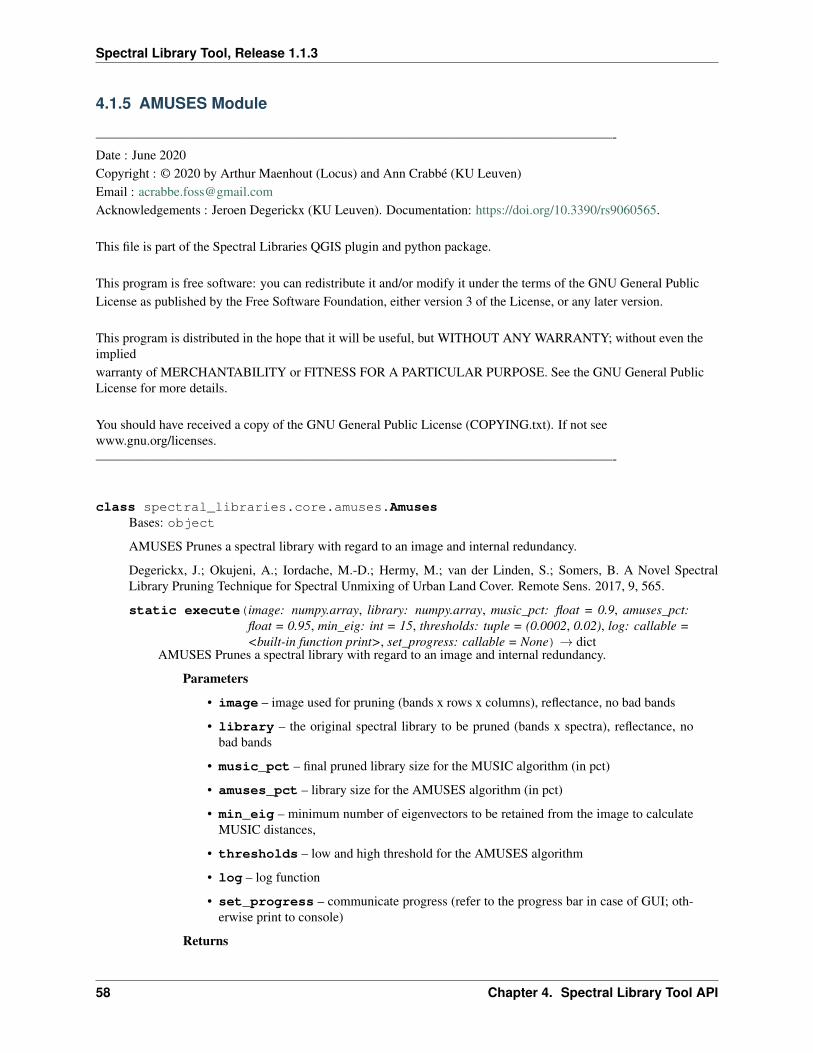
Spectral Library Tool, Release 1.1.3
4.1.5 AMUSES Module
———————————————————————————————————————-Date : June 2020Copyright : © 2020 by Arthur Maenhout (Locus) and Ann Crabbé (KU Leuven)Email : [email protected] : Jeroen Degerickx (KU Leuven). Documentation: https://doi.org/10.3390/rs9060565.
This file is part of the Spectral Libraries QGIS plugin and python package.
This program is free software: you can redistribute it and/or modify it under the terms of the GNU General PublicLicense as published by the Free Software Foundation, either version 3 of the License, or any later version.
This program is distributed in the hope that it will be useful, but WITHOUT ANY WARRANTY; without even theimpliedwarranty of MERCHANTABILITY or FITNESS FOR A PARTICULAR PURPOSE. See the GNU General PublicLicense for more details.
You should have received a copy of the GNU General Public License (COPYING.txt). If not seewww.gnu.org/licenses.———————————————————————————————————————-
class spectral_libraries.core.amuses.AmusesBases: object
AMUSES Prunes a spectral library with regard to an image and internal redundancy.
Degerickx, J.; Okujeni, A.; Iordache, M.-D.; Hermy, M.; van der Linden, S.; Somers, B. A Novel SpectralLibrary Pruning Technique for Spectral Unmixing of Urban Land Cover. Remote Sens. 2017, 9, 565.
static execute(image: numpy.array, library: numpy.array, music_pct: float = 0.9, amuses_pct:float = 0.95, min_eig: int = 15, thresholds: tuple = (0.0002, 0.02), log: callable =<built-in function print>, set_progress: callable = None)→ dict
AMUSES Prunes a spectral library with regard to an image and internal redundancy.
Parameters
• image – image used for pruning (bands x rows x columns), reflectance, no bad bands
• library – the original spectral library to be pruned (bands x spectra), reflectance, nobad bands
• music_pct – final pruned library size for the MUSIC algorithm (in pct)
• amuses_pct – library size for the AMUSES algorithm (in pct)
• min_eig – minimum number of eigenvectors to be retained from the image to calculateMUSIC distances,
• thresholds – low and high threshold for the AMUSES algorithm
• log – log function
• set_progress – communicate progress (refer to the progress bar in case of GUI; oth-erwise print to console)
Returns
58 Chapter 4. Spectral Library Tool API

Spectral Library Tool, Release 1.1.3
dictionary with each output metric as a numpy array in a key-value pair - music_indices:library indices after pruning with the MUSIC algorithm - music_eigenvectors: first kf eigen-vectors of image subspace (needed for sparse unmixing)
kf = estimated number of eigenvectors in the image estimated by Hysime algorithm
• music_distances: MUSIC distances of the pruned library spectra to the image, sorted fromlow to high
• amuses_indices: library indices after pruning with the AMUSES algorithm
spectral_libraries.core.amuses.printProgress(value: int)Replacement for the GUI progress bar
See the User Guide for instructions on using the Command Line Interface.
4.1. Spectral Library Optimization 59

Spectral Library Tool, Release 1.1.3
60 Chapter 4. Spectral Library Tool API
CHAPTER 5
About The Spectral Library Tool
The Spectral Library Tool software package is both a QGIS plugin and stand-alone python package that provides asuite of processing tools for multi- and hyperspectral spectral libraries.
The software is based on VIPER Tools: code written for ENVI/IDL and released in 2007. Several updates have beenreleased since and now it has been ported to PyQGIS in the period 2017 - 2020. The original VIPER Tools is now splitover two python/QGIS tools: Spectral Library Tools and MESMA.
Spectral Library Tool provides the following:
• Creating spectral libraries interactively (selecting spectra from an image or using regions of interest) andmanaging the metadata (developed by HU Berlin)
• Optimizing spectral libraries with Iterative Endmember Selection, Ear-Masa-Cob, CRES, MUSIC orAMUSES
• Website: <https://spectral-libraries.readthedocs.io>
• Repository: https://bitbucket.org/kul-reseco/spectral-libraries
MESMA provides the following:
• Running SMA and MESMA (with multi-level fusion, stable zone unmixing, . . . )
• Post-processing of the MESMA results (visualisation tool, shade normalisation, . . . )
• Website: <https://mesma.readthedocs.io>
• Repository: https://bitbucket.org/kul-reseco/mesma
The software has now been developed in the open source environment to encourage further development of the tool.
PLEASE GIVE US CREDIT
When using The Spectral Library Tool, please use the following citation:
Crabbé, A. H., Jakimow, B., Somers, B., Roberts, D. A., Halligan, K., Dennison, P., Dudley, K. (2020). SpectralLibrary QGIS Plugin (Version x) [Software]. Available from https://bitbucket.org/kul-reseco/spectral-libraries.
ACKNOWLEDGEMENTS
61

Spectral Library Tool, Release 1.1.3
The software and user guide are based on VIPER Tools 2.0 (UC Santa Barbara, VIPER Lab): Roberts, D. A., Halligan,K., Dennison, P., Dudley, K., Somers, B., Crabbe, A., 2018, Viper Tools User Manual, Version 2, 91 pp.
The software also makes use of the QGISPluginSupport python packages developed by Benjamin Jakimow (HUBerlin): https://bitbucket.org/jakimowb/qgispluginsupport.
The MUSIC and AMUSES algorithms are based on work and code by Jeroen Degerickx (KU Leuven): https://doi.org/10.3390/rs9060565.
This revision is funded primarily through BELSPO (the Belgian Science Policy Office) in the framework of theSTEREO III Programme – Project LUMOS - SR/01/321.
Logo’s were created for free at https://logomakr.com.
SOFTWARE LICENSE
This program is free software: you can redistribute it and/or modify it under the terms of the GNU General PublicLicense as published by the Free Software Foundation, either version 3 of the License, or any later version.
This program is distributed in the hope that it will be useful, but WITHOUT ANY WARRANTY; without even theimplied warranty of MERCHANTABILITY or FITNESS FOR A PARTICULAR PURPOSE. See the GNU GeneralPublic License for more details.
You should have received a copy of the GNU General Public License (COPYING.txt). If not seewww.gnu.org/licenses.
5.1 Indexes
• genindex
• modindex
62 Chapter 5. About The Spectral Library Tool

Bibliography
[BioucasDias2008] Bioucas-Dias JM, Nascimento JMP. 2008. Hyperspectral Subspace Identification. IEEE Transac-tions on Geoscience and Remote Sensing, volume 46, p. 2435-2445.
[Clark2005] Clark M. 2005. An assessment of Hyperspectral and Lidar Remote Sensing for the Monitoring of TropicalRain Forest Trees. University of California, Santa Barbara, 319 pp.
[Degerickx2016] Degerickx J, Iordache MD, Okujeni A, Hermy M, van der Linden S, Somers B. 2016. Spectralunmixing of urban land cover using a generic library approach. In Proceedings of the SPIE 10008, RemoteSensing Technologies and Applications in Urban Environments, Edinburgh, UK, 26 September 2016.
[Degerickx2017] Degerickx J, Okujeni A, Iordache M-D, Hermy M, van der Linden S, Somers B. 2017. A NovelSpectral Library Pruning Technique for Spectral Unmixing of Urban Land Cover. Remote Sensing, vol-ume 9, 565.
[Dennison2003] Dennison PE, Roberts DA. 2003. The Effects of Vegetation Phenology on Endmember Selectionand Species Mapping in Southern California Chaparral. Remote Sensing of Environment, volume 87, p.295-309.
[Dennison2004] Dennison PE, Halligan KQ and Roberts DA. 2004. A Comparison of Error Metrics and Constraintsfor Multiple Endmember Spectral Mixture Analysis and Spectral Angle Mapper. Remote Sensing ofEnvironment, volume 93, p. 359-367.
[Dudley2015] Dudley KL, Dennison PE, Roth KL, Roberts DA and Coates AR. 2015. A Multitemporal SpectralLibrary Approach for Mapping Vegetation Species Across Spatial and Temporal Phenological Gradients.Remote Sensing of Environment, volume 167, p. 121-134.
[Fernandez2016] Fernandez-Manso A, Quintano C and Roberts DA. 2016. Burn severity influence on post-fire vege-tation cover resilience from Landsat MESMA fraction images time series in Mediterranean forest ecosys-tems. Remote Sensing of Environment, volume 184, p. 112-123.
[Gardner1997] Gardner M. 1997. Mapping chaparral with AVIRIS using Advanced Remote Sensing Techniques.University of California, Santa Barbara, 58 pp.
[Halligan2002] Halligan KQ. 2002. Multiple Endmember Spectral Mixture Analysis of Vegetation in the NortheastCorner of Yellowstone National Park. University of California, Santa Barbara, 64 pp.
[Iordache2014] Iordache MD, Bioucas-Dias JM, Plaza A, Somers B. 2014. MUSIC-CSR: Hyperspectral unmixingvia multiple signal classification and collaborative sparse regression. IEEE Transactions on Geoscienceand Remote Sensing, volume 52, p. 4364-4382.
63

Spectral Library Tool, Release 1.1.3
[Padma2014] Padma S, Sanjeevi S. 2014. Jeffries Matusita based mixed-measure for improved spectral matching inhyperspectral image analysis. International Journal of Applied Earth Observation and Geoinformation,volume 32, p. 138-151.
[Quintano2017] Quintano C, Fernandez-Manso A and Roberts DA. 2017. Burn severity mapping from LandsatMESMA fraction images and Land Surface Temperatures. Remote Sensing of Environment, volume 190,p. 83-95.
[Roberts1993] Roberts DA, Adams JB and Smith MO. 1993. Discriminating Green Vegetation, Non-PhotosyntheticVegetation and Soils in AVIRIS Data. Remote Sensing of Environment, volume 44, p. 255-270.
[Roberts1997] Roberts DA, Gardner ME, Church R Ustin SL and Green RO. Optimum Strategies for Mapping Veg-etation using Multiple Endmember Spectral Mixture Models. Proceedings of the SPIE, volume 3118, p.108-119.
[Roberts1998] Roberts DA, Gardner M, Church R, Ustin S, Scheer G and Green RO. 1998. Mapping Chaparral inthe Santa Monica Mountains using Multiple Endmember Spectral Mixture Models, Remote Sensing ofEnvironment, volume 65, p. 267-279.
[Roberts2002] Roberts DA, Numata I, Holmes KW, Batista G, Krug T, Monteiro A, Powell B and Chadwick O. 2002.Large area mapping of land-cover change in Rondônia using multitemporal spectral mixture analysis anddecision tree classifiers. Journal of Geophysical Research: Atmospheres, volume 107, p. 40-1 to 40-18.
[Roberts2003] Roberts DA, Dennison PE, Gardner M, Hetzel Y, Ustin SL and Lee C. 2003. Evaluation of the Po-tential of Hyperion for Fire Danger Assessment by Comparison to the Airborne Visible/Infrared ImagingSpectrometer. IEEE Transactions on Geoscience and Remote Sensing, volume 41, p. 1297-1310.
[Roberts2004] Roberts DA, Ustin SL, Ogunjemiyo S, Greenberg J, Dobrowski SZ, Chen J and Hinckley TM. 2004.Spectral and structural measures of Northwest forest vegetation at leaf to landscape scales, Ecosystems,volume 7, p. 545-562.
[Roberts2015] Roberts DA, Dennison PE, Roth KL, Dudley K and Hulley G. 2015. Relationships Between DominantPlant Species, Fractional Cover and Land Surface Temperature in a Mediterranean Ecosystem. RemoteSensing of Environment, volume 167, p. 152-167.
[Roth2012] Roth KL, Dennison PE and Roberts DA. 2012. Comparing endmember selection techniques for accuratemapping of plant species and land cover using imaging spectrometer data. Remote Sensing of Environ-ment, volume 127, p. 139-152.
[Roth2015] Roth KL, Roberts DA, Dennison PE, Alonzo M, Peterson SH and Beland M. 2015. Differentiating PlantSpecies within and across Diverse Ecosystems with Imaging Spectroscopy. Remote Sensing of Environ-ment, volume 167, p. 135-151.
[Schaaf2011] Schaaf AN, Dennison PE, Fryer GK, Roth KL and Roberts DA. 2011. Mapping Plant Functional Typesat Multiple Spatial Resolutions using Imaging Spectrometer Data. GIScience Remote Sensing, volume48, p. 324-344.
[Wu2004] Wu C. 2004. Normalized spectral mixture analysis for monitoring urban composition using ETM+ im-agery. Remote Sensing of Environment, volume 93, p. 480-492.
[Herold2004] Herold M, Roberts DA, Gardner ME and Dennison PE. 2004. Spectrometry for urban area remotesensing – Development and analysis of a spectral library from 350 to 2400 nm. Remote Sensing of Envi-ronment, volume 91, p. 304-319.
[Roberts2003] Roberts DA, Dennison PE, Gardner M, Hetzel Y, Ustin SL and Lee C. 2003. Evaluation of the Po-tential of Hyperion for Fire Danger Assessment by Comparison to the Airborne Visible/Infrared ImagingSpectrometer. IEEE Transactions on Geoscience and Remote Sensing, volume 41, p. 1297-1310.
[Roberts2015] Roberts DA, Dennison PE, Roth KL, Dudley K and Hulley G. 2015. Relationships Between DominantPlant Species, Fractional Cover and Land Surface Temperature in a Mediterranean Ecosystem. RemoteSensing of Environment, volume 167, p. 152-167.
64 Bibliography

Spectral Library Tool, Release 1.1.3
[Roberts2017] Roberts DA, Alonzo M, Wetherley E, Dudley K and Dennison P. 2017. Scale in Remote Sensing andGIScience Applications. Chapter: Multiscale Analysis of Urban Areas using Mixing Models, p. 247-282.
[Roth2012] Roth KL, Dennison PE and Roberts DA. 2012. Comparing endmember selection techniques for accuratemapping of plant species and land cover using imaging spectrometer data. Remote Sensing of Environ-ment, volume 127, p. 139-152.
Bibliography 65

Spectral Library Tool, Release 1.1.3
66 Bibliography

Python Module Index
sspectral_libraries.core.amuses, 58spectral_libraries.core.cres, 54spectral_libraries.core.ear_masa_cob,
51spectral_libraries.core.ies, 53spectral_libraries.core.music, 56
67

Spectral Library Tool, Release 1.1.3
68 Python Module Index
Index
AAmuses (class in spectral_libraries.core.amuses), 58
CCres (class in spectral_libraries.core.cres), 54
EEarMasaCob (class in spec-
tral_libraries.core.ear_masa_cob), 52estimate_noise() (spec-
tral_libraries.core.music.Music method),56
execute() (spectral_libraries.core.amuses.Amusesstatic method), 58
execute() (spectral_libraries.core.cres.Cres method),55
execute() (spectral_libraries.core.ear_masa_cob.EarMasaCobstatic method), 52
execute() (spectral_libraries.core.ies.Ies method), 53execute() (spectral_libraries.core.music.Music
method), 57
Fflatten_image() (spec-
tral_libraries.core.music.Music static method),57
Gget_fractions() (spectral_libraries.core.cres.Cres
method), 55get_header() (spectral_libraries.core.cres.Cres
method), 55
Hhysime2() (spectral_libraries.core.music.Music
method), 57
IIes (class in spectral_libraries.core.ies), 53
index() (spectral_libraries.core.cres.Cres method), 55
MMusic (class in spectral_libraries.core.music), 56
Nnormalize_brightness() (spec-
tral_libraries.core.music.Music static method),57
PprintProgress() (in module spec-
tral_libraries.core.amuses), 59printProgress() (in module spec-
tral_libraries.core.ies), 54
Sspectral_libraries.core.amuses (module),
58spectral_libraries.core.cres (module), 54spectral_libraries.core.ear_masa_cob
(module), 51spectral_libraries.core.ies (module), 53spectral_libraries.core.music (module), 56
69


![CRISM Data Users' Workshop Nili Fossae Data Processing ......Smectite PHY07_02 [Link to Spectral Library] Smectite PHY07 [Link to Spectral Library] 03/22/2009 CRISM Workshop - Data](https://img.pdfslide.net/doc/110x75/60b27f7c389ce535bc442a75/crism-data-users-workshop-nili-fossae-data-processing-smectite-phy0702.jpg)