Spectral Processing of Tangential Vector Fields · 2016-05-26 · Spectral mesh processing Within the last decade a large num-ber of methods for tasks in shape analysis and processing

Volume 35 (2016), Number 2 pp. 1–14 COMPUTER GRAPHICS forum

Spectral Processing of Tangential Vector Fields

Christopher Brandt Leonardo Scandolo Elmar Eisemann Klaus Hildebrandt

Delft University of Technology

Abstract

We propose a framework for the spectral processing of tangential vector fields on surfaces. The basis is a Fourier-type repre-sentation of tangential vector fields that associates frequencies with tangential vector fields. To implement the representationfor piecewise constant tangential vector fields on triangle meshes, we introduce a discrete Hodge–Laplace operator that fitsconceptually to the prominent cotan discretization of the Laplace–Beltrami operator. Based on the Fourier representation, weintroduce schemes for spectral analysis, filtering and compression of tangential vector fields. Moreover, we introduce a spline-type editor for modeling of tangential vector fields with interpolation constraints for the field itself and its divergence and curl.Using the spectral representation, we propose a numerical scheme that allows for real-time modeling of tangential vector fields.

Categories and Subject Descriptors (according to ACM CCS): I.3.5 [Computer Graphics]: Computational Geometry and ObjectModeling—

1. Introduction

Tangential vector fields are a fundamental representation of direc-tional information on a surface. For example, gradients of functionsare tangential vector fields and flows, stresses, strains, or curvaturedirections are tangential to a surface. Therefore, the processing oftangential vector fields is important for algorithms for many appli-cations in graphics.

Spectral methods are well established for the processing of func-tions and signals over planar domains. Within the last decade, spec-tral methods for the processing of curved surfaces and functionson them have been developed and the field of spectral mesh pro-cessing has been established. Central is the eigendecomposition ofthe Laplace–Beltrami operator, which generalizes the Fourier basisfrom planar domains to curved surfaces. Whereas on planar do-mains, spectral methods can be directly generalized to the process-ing of vector fields by simply applying the method to each of thecomponent functions of the vector field, this is not possible for tan-gential vector fields on curved surfaces because there is no rigidCartesian coordinate system.

In this paper, we introduce a framework for spectral processingof tangential vector fields on curved surfaces. The foundation is aFourier-type representation that associates frequencies with tangen-tial vector fields. To construct the Fourier-type basis on the space oftangential vector fields, we combine the eigendecomposition of theHodge–Laplace operator and the Hodge decomposition to obtainbasis fields that are either integrable, co-integrable or harmonic.

We formulate the spectral processing framework for piecewiseconstant tangential vector fields on triangle meshes. These vector

fields are widely used in graphics applications and a discrete Hodgedecomposition has been established. To define the spectral basis,we introduce a discrete Hodge–Laplace operator for piecewise con-stant vector fields on surface meshes. The operator shares importantproperties with its continuous counterpart and fits conceptually tothe prominent cotan discretization of the Laplace–Beltrami opera-tor. We show that a sparse matrix representation of the operator canbe obtained by combining a set of simple matrices. Additionally, wederive a discrete Dirichlet energy that can be used as a regularizeror fairness energy for piecewise constant tangential vector fieldson surfaces. For solving the eigenproblem of the discrete Hodge–Laplace operator, we introduce a scheme that boils the computationof the eigenfields down to the computation of the eigenfunctions oftwo discrete Laplace–Beltrami operators.

To illustrate the potential of our framework for the applications,we introduce tools for spectral filtering and analysis, compressionand real-time tangential vector field design. The filtering tools al-low users to design filters in the spectral domain. Individual filterscan be specified for the integrable and co-integrable parts of a field.The compression scheme allows for lossy compression of tangen-tial vector fields at high compression rates. For vector field design,we follow the approach introduced by Fisher et al. [Fisher2007].A tangential vector field is constructed by minimizing the Dirich-let energy subject to soft constraints that implement the user input.We demonstrate that by restricting the design space to the spacespanned by 1-2k low-frequency eigenfields, the computation is sig-nificantly accelerated (up to a factor of 200 in our experiments).

Our second main contribution is a “spline-like”-editor for tan-

c© 2016 The Author(s)Computer Graphics Forum c© 2016 The Eurographics Association and JohnWiley & Sons Ltd. Published by John Wiley & Sons Ltd.

C. Brandt, L. Scandolo, E. Eisemann & K. Hildebrandt / Spectral Processing of Tangential Vector Fields

gential vector fields. It allows for modeling tangential vector fieldsusing hard constraints on the field and its divergence and curl. Tan-gential vector field splines (TVFS) can be defined (analogous tocubic splines) as the minimizers of a biharmonic energy under con-straints. This idea was already discussed in [Fisher2007] as a pos-sible extension of the design method introduced in the paper. How-ever their approach has two limitations: only soft constraints canbe imposed and the resulting scheme is not fast enough to allowfor interactive editing. In this work, we overcome both limitationsand transfer the approach to piecewise constant vector fields. Tobe able to formulate TVFS for piecewise constant vector fields, weintroduce a biharmonic energy for these fields. Furthermore, we in-troduce a numerical scheme for computing the TVFS in real-time.The scheme combines the spectral basis and an efficient solver ofthe quadratic problem. The supplementary video illustrates the ben-efits of hard constraints for vector field modeling. A live editingsession demonstrates the benefit of the TVFS editor for the designof fur on meshes.

We want to remark that after the submission of this paper wefound that concurrently to our work the discrete Hodge–Laplaceoperator for piecewise constant vector fields was also introducedin [dGDT15] and a scheme for computing the eigenfields usingeigenfunctions was introduced in [LMH∗15], also concurrent tothis work.

2. Related Work

Spectral mesh processing Within the last decade a large num-ber of methods for tasks in shape analysis and processing that usethe spectrum and eigenfunctions of the Laplace–Beltrami opera-tor have been proposed. In the following, we briefly discuss someof the applications. For an introduction to spectral mesh process-ing and a broader overview of applications, we refer to the sur-veys by Lévy and Zhang [LZ09] and Zhang, van Kaick and Dyer[ZvKD10].

The eigendecomposition of the Laplace–Beltrami operatoryields a basis of the space of functions on a curved surface anal-ogous to the Fourier basis for signals over a one-dimensional do-main. By transforming a function into this basis, it is decomposedinto oscillations that are ordered by their frequencies. Even the sur-face itself (i.e., the embedding of the surface in R3) can be treatedin this way. Vallet and Lévy [VL08] proposed a framework for thedesign of mesh filters. The framework allows for amplifying andsuppressing the different frequencies in the embedding of the mesh.For example, high and low pass filters for sharpening and smooth-ing the mesh can be constructed. Karni and Gotsman [KG00] pro-posed a scheme for the compression of triangle meshes based onthe eigendecomposition of a combinatorial Laplacian. Recently, ascheme for the compression of dynamic mesh sequences was in-troduced by Váša et al. [VMHB14]. The regular pattern of min-ima and maxima of the eigenfunctions are used for generating aquadrangular mesh on a surface. Dong et al. [DBG∗06] introducea technique that uses the Morse–Smale complex of a carefully cho-sen eigenfunction to generate a coarse quadrangulation. Huang etal. [HZM∗08] and Ling et al. [LHJ∗14] extended this approachsuch that it can provide a user with control of the shape, size, orien-tation, and feature alignment of the faces of the resulting quadran-

gulation. Spectral methods for shape segmentation have been intro-duced by Sharma et al. [SHKvL09] and Huang et al. [HWAG09].

The eigenfunctions enjoy many desirable properties. They areintrinsic, which means they do not change if the mesh is iso-metrically deformed. Since they are derived as the discretizationof a continuous concept, they are mesh independent. They arevariational, which makes them robust to remeshing. These prop-erties make them well-suited for the design of pose-independentand mesh-independent shape descriptors. Various descriptors havebeen designed including the Shape-DNA introduced by Reuter etal. [RWP05, RWP06], Rustamov’s Global Point Signature (GPS)[Rus07], the Heat Kernel Signature (HKS) proposed by Sun etal. [SOG09], the Auto Diffusion Function introduced by Gebalet al. [GBAL09] and the Wave Kernel Signature by Aubry etal. [ASC11]. A signature involving not only intrinsic, but also ex-trinsic information about the surface was introduced in [HSvTP10,HSvTP12]. Based on the GPS and the HKS, Ovsjanikov etal. [OSG08, OMMG10] introduced schemes for the detection ofshape symmetries. The pose and mesh independence has also beenthe basis of schemes for shape correspondences and matching. Deyet al. [DLL∗10] propose a robust pose-oblivious shape matchingalgorithm based on persistent extrema of the HKS. The functionalmaps framework, introduced by Ovsjanikov at el. [OBCS∗12], useslow-frequency eigenfunctions of the Laplace–Beltrami operator ontwo shapes for constructing a linear map between the functionspaces of the shapes. Rustamov et al. [ROA∗13] used this func-tional correspondence to compare shapes.

Discrete Laplace–Beltrami operators are the backbone of spec-tral mesh processing. Commonly, piecewise linear and continuousfunctions (linear Lagrange finite elements) over triangle meshes areconsidered. The discretization of the Laplace–Beltrami operator inthis setting leads to the prominent cotan weights [PP93,MDSB03].Discretizations with higher-order elements were consider by Reuteret al. [RWP05]. Properties of the discrete Laplace operators havebeen studied by Wardetzky et al. [WMKG07,AW11]. Convergenceof the discrete operators and their spectrum have been studied byHildebrandt et al. [HPW06, HP11] and Dey et al. [DRW10].

In this paper, we are proposing a framework that allows forapplying spectral methods for the processing of tangential vectorfields on surface meshes. The spectral analysis of vector fieldson planar domains has been treated by Wagner, Garth and Ha-gen [WGH12] and a construction of reduced bases for fluid sim-ulation on planar domains using Laplace eigenfunctions was intro-duced by de Witt, Lessig and Fiume [DWLF12]. These techniqueshowever do not carry over to curved surfaces since they require afixed Cartesian coordinate system, which is not available for tan-gential fields on curved surfaces.

Tangential vector field processing Tangential vector fields ap-pear in many applications in graphics. They are used for control-ling anisotropic shading of surfaces [MRMH12, RGB∗14], non-photorealistic rendering [HZ00, YCLJ12, CYZL14], texture gener-ation [WL01, KCPS15], simulation of fluid and liquids on surfaces[AWO∗14, AVW∗15], surface segmentation [SBCBG11, ZZCJ14]and surface construction [IBB15, PLS∗15]. For a recent surveyson direction field synthesis, design, and processing, we referto [dGDT15, VCD∗16]. Methods that use tangential vector fields

c© 2016 The Author(s)Computer Graphics Forum c© 2016 The Eurographics Association and John Wiley & Sons Ltd.


and more general direction fields for surface meshing have receivedmuch attention in recent years. Some examples are [RLL∗06,KNP07, BZK09, LLZ∗11, TPP∗11, ECBK14, CK14, LLW15]. Fora recent survey on the topic, we refer to [BLP∗13].

The Hodge decomposition of vector fields is an important toolfor the processing of tangential vector fields. It allows for decom-posing the fields into an integrable, a co-integrable and a harmonicpart. A discrete Hodge decomposition of the space of piecewiseconstant vector fields on a surface mesh has been introduced byPolthier and Preuss [PP00, PP03]. Tong et al. [TLHD03] general-ized this decomposition to 3-dimensional domains and introduceda multi-resolution representation of vector fields using the potentialand co-potential of a vector field. Wardetzky [War06] extended theapproach from simply-connected domains to surfaces of arbitrarygenus and proved convergence of the decomposition. The spectraldecomposition we are proposing is compatible with this discreteHodge decomposition. For a recent survey on discretizations andapplications of the Hodge decomposition, we refer to [BNPB13].

Fairness energies are used for the reconstruction, design and syn-thesis of tangential vector and direction fields. Fairness energies fordifferent representations of vector and direction fields have beenproposed [ZMT06,ZHT07,RVLL08,BZK09,KCPS13,DVPSH14].Here, we introduce a discretization of the Dirichlet energy forpiecewise constant tangential vector fields using a combination ofconforming and non-conforming discrete divergence and curl op-erators.

Alternatively to working with vector fields, one can dualizeand consider 1-forms. Discrete Exterior Calculus [DHLM05] pro-vides notions of discrete k-forms and discrete operators on themincluding a discrete Hodge Laplacian for k-forms. A discreteHodge decomposition for 1-forms was introduced by Fisher etal. [FSDH07] and a spectral decomposition of a discrete HodgeLaplacian on spaces of discrete k-forms has been derived by Arnoldet al. [AFW06].

3. Background: Hodge Decomposition of Vector Fields

In this section, we review the Hodge decomposition of vector fieldson a smooth surface M embedded in R3. We denote the surfacenormal field by N, and, for any point p ∈ M the tangent planeofM at p by TpM. Before stating the Hodge decomposition, weintroduce basic differential operators on the space of functions andvector fields on surfaces.

Gradient, divergence, curl and Laplace–Beltrami The gradientis a linear operator mapping differentiable functions to tangentialvector fields. For any point p ∈M the gradient of f at p is definedas the tangential vector grad f (p) that satisfies

〈grad f (p),v〉R3 = dv f (p)

for all v ∈ TpM. Here, dv f (p) is the derivative of f at p in direc-tion v. At any point, grad f points in direction of the steepest ascentof f . We denote by J the operator that rotates any vector of a vec-tor field in its tangent plane by π

2 (following the orientation of thesurface). Besides the gradient operator, we consider the operatorJ grad, which concatenates the gradient and the rotation J. We callthis operator the co-gradient.

The divergence and curl are linear operators that map vectorfields to functions. The divergence of a vector field v at a pointp ∈M is defined by

div v(p) =2

∑i=1〈∇ei v(p),ei〉,

where∇ is the covariant derivative and {e1,e2} forms an orthogo-nal basis of the tangent plane at p. We define the curl as

curl v =−div J v. (1)

The divergence and curl are related to the gradient and co-gradient.To describe this relation, we use the L2-scalar products on thespaces of square-integrable functions and vector fields. These aredefined as

〈 f ,g〉L2 =∫M

f (p)g(p)dA (2)

〈v,w〉L2 =∫M〈v(p),w(p)〉R3 dA (3)

The divergence and gradient as well as the curl and the co-gradientsatisfy

〈divv, f 〉L2 =−〈v,grad f 〉L2 (4)

〈curl v, f 〉L2 =−〈v,Jgrad f 〉L2 , (5)

for all pairs of a continuously differentiable function f and tan-gential vector field v, which follows from an integration by parts.By combining the operators introduced above, we can define theLaplace–Beltrami operator

∆ =−divgrad (6)

on the space of twice differentiable functions. Note that the opera-tor could alternatively be defined as the negative of the curl of theco-gradient: ∆ =−curl Jgrad.

Hodge decomposition and harmonic fields The space X ofsmooth tangential vector fields on a surface with vanishing bound-ary can be decomposed into three L2-orthogonal subspaces

X = Image(grad)⊕ Image(J grad)⊕H,

The first subspace is formed by the gradients of smooth functions.Fields in this space are curl-free and represent the integrable partof a vector field. Similarly, the second subspace is the space ofco-gradients of smooth functions, which are divergence-free. Thisspace represents the co-integrable part of a vector field. The thirdspace consists of the harmonic tangential vector fields H. Thesefields are neither gradients nor co-gradients of functions. The spaceH can be defined as the intersection of the kernel of the diver-gence and the curl. In other words, these are exactly the fields thathave vanishing divergence and curl. The space contains informa-tion about the topology of the surface. H equals the first singularcohomology of the surface. This is an important relation betweenvector calculus and algebraic topology. We refer to the literature,e.g. [War13], for more about this connection. One consequence isthat the dimension ofH on a surface of genus g is 2g.

4. Discrete Hodge Decomposition

In graphics applications, we are often dealing with piecewise con-stant vector fields on triangle meshes. A discrete counterpart of the



Hodge decomposition for piecewise constant vector fields has beenintroduced in [PP00, PP03, TLHD03, War06]. In this section, wereview this construction.

Function spaces We denote the space of vector fields that are con-stant in every triangle of a meshMh by Xh. In addition, we con-sider two function spaces. Both consist of functions on Mh thatare linear polynomials in every triangle. The two spaces are con-structed by imposing continuity constraints on the linear polynomi-als of neighboring triangles: the space Sh of piecewise linear poly-nomials that are globally continuous and the space S∗h of piecewiselinear polynomials that are continuous at the midpoints of all inte-rior edges. The combination of Sh and S∗h is needed for the discreteHodge decomposition.

Discrete operators The gradients of functions in Sh and S∗h are de-fined for all points in the interior of a triangle and they are constantwithin each triangle. Hence the gradient is a linear map from Shand S∗h into Xh. While the gradient can be directly transferred tothe discrete setting, we define the discrete divergence and curl op-erators indirectly using the gradient and equations (4) and (5). Asin the continuous case, the discrete divergence and curl map vectorfields to functions. Since we are working with two function spaces,we get two discrete divergence and curl operators. The conformingdiscrete divergence is the linear operator

divh : Xh 7→ Sh

that satisfies

〈divhv, f 〉L2 =−〈v,grad f 〉L2

for all v ∈ Xh and f ∈ Sh and the nonconforming discrete diver-gence is the linear operator

div∗h : Xh 7→ S∗h

that satisfies ⟨div∗h v,g

⟩L2 =−〈v,grad g〉L2

for all v ∈ Xh and g ∈ S∗h . Following the definition (1) of the curlin the continuous case, the conforming and nonconforming discretecurl operators are defined as

curlhv =−divhJv and curl∗h v =−div∗h Jv.

We discuss explicit matrix representations of the operators in Sec-tion 5.

Finally, we want to remark that there is a difference betweenthe discrete operators we define here and the definitions in [PP03,War06]. They define the divergences and curls of vector fields asintegrated quantities, while in the presented definitions, the diver-gences and curls of vector fields are piecewise linear functions(hence pointwise quantities). The notions are related, one can usethe mass matrix (see Section 5) to convert one into the other. We re-fer to [WBH∗07] for a discussion of integrated vs. pointwise quan-tities.

Discrete Hodge decomposition As in the continuous case, the dis-crete Hodge decomposition divides the space of vector fields intothree orthogonal subspaces: the image of the gradient, the image

of the co-gradient and a space of harmonic vector fields. To ob-tain spaces of harmonic fields that are 2g-dimensional as in thecontinuous case, we need to combine the spaces Sh and S∗h . Thediscrete Hodge decomposition of the space of piecewise constantvector fields is

Xh = Image(grad|Sh)⊕ Image(J grad|S∗

h)⊕Hh. (7)

The first component, Image(grad|Sh), consists of the vector fields

that are gradients of functions in Sh. This part describes the inte-grable part of a vector field, which has vanishing nonconformingdiscrete curl. This means the first component is part of the ker-nel of curl∗h . The second component, Image(J grad|S∗

h), consists of

the vector fields that are co-gradients of functions in S∗h , the co-integrable part. These vector fields have vanishing conforming dis-crete divergence. Hence, the second component is part of the kernelof divh. For surfaces with genus zero (homeomorphic to a sphere),Image(grad|Sh

) is exactly the kernel of curl∗h and Image(J grad|S∗h)

is exactly the kernel of divh. However, for surfaces with non-vanishing genus g there is a 2g-dimensional spaceHh of piecewiseconstant vector fields for which curl∗h and divh vanish. These vec-tor fields are neither gradients of functions in Sh nor co-gradientsof functions in S∗h . We call

Hh = Kernel(divh)∩Kernel(curl∗h )

the space of discrete harmonic vector fields.

We want to emphasize that this theory requires the interplay ofthe conforming and nonconforming spaces and operators. For ex-ample, a vector field is the gradient of a function in Sh (on a simply-connected domain) if curl∗h vanishes. Moreover, to get spaces ofdiscrete harmonic vector fields of dimension 2g, the spaces Sh andS∗h have to be combined. If only gradients and co-gradients of func-tions in Sh are used, the dimension of the resulting space of har-monic fields depend on the mesh (and not only on the genus of thesurface) and are usually large (e.g. the dimension grows under meshrefinement).

As an alternative to (7), we could exchange theroles of Sh and S∗h and obtain the decompositionXh =Image(grad|S∗

h)⊕Image(J grad|Sh

) ⊕ H∗h . Since in thiscase the integrable part of a vector field is the gradient of afunction in S∗h , we call this the nonconforming discrete Hodgedecomposition. The resulting space of nonconforming discreteharmonic fields is H∗h =Kernel(div∗h )∩Kernel(curlh). The fact thatthere are two different discrete Hodge decompositions is specificto the discrete setting and is not present in the continuous case.In [War06], it was shown that both decompositions converge totheir smooth counterpart under suitable refinement of the surfacemeshes. In this sense, the two decompositions are similar.

In the following, we will consider only the decomposition (7).However, for any notion we introduce, there is a corresponding no-tion where the roles of the spaces Sh and S∗h are exchanged.

5. Discrete Hodge–Laplace Operator for Vector Fields

In this section, we introduce a discrete Hodge–Laplace operatorfor piecewise constant vector fields on surface meshes and the cor-responding discrete Dirichlet and biharmonic energies. Before weconsider the discrete setting, we first review the smooth setting.



The smooth setting By combining the operators discussed in Sec-tion 3, one can construct the Hodge–Laplace operator

∆ =−(grad div+ J grad curl) (8)

on the space of smooth tangential vector fields on a surface. Weuse the minus sign in (8) to get positive eigenvalues for the Hodge–Laplace operator.

Since we could not find a reference where (8) is stated, we wantto put this formula in context with the literature (the supplementarymaterial includes a more detailed derivation). The Hodge Laplacianis usually defined as an operator on smooth k-forms on a Rieman-nian manifold [AF02]. For surfaces, 0- and 2-forms can be identi-fied with functions and the Hodge Laplacian for these forms is theLaplace–Beltrami operator (6) for functions. 1-forms on a surfacecan be identified with vector fields via v↔ 〈v, ·〉. Using this iso-morphism, we can carry over the Hodge Laplacian from 1-forms tovector fields and express this operator in terms of the operators J,grad, div and curl. Formula (8) is the resulting operator. For vec-tor fields on planar domains, this operator agrees with the vectorLaplacian. In this sense, the Hodge Laplacian generalizes the vectorLaplacian from vector fields on planar domain to tangential vectorfields on curved surfaces.

Discrete Hodge–Laplace operators Using the definition (8) ofthe smooth Hodge–Laplace operator for tangential vector fields ona surface and the discrete operators introduced in Section 4, wecan construct the discrete Hodge–Laplace operator for piecewiseconstant vector fields on a surface mesh. As for the discrete Hodgedecomposition, the discretization mixes the conforming discrete di-vergence and the non-conforming discrete curl operators

∆h =−(grad divh + J grad curl∗h ).

The discrete Hodge–Laplace operator ∆h shares many propertieswith its continuous counterpart ∆.

1. Symmetry The operator ∆h is self-adjoint with respect to theL2-scalar product, i.e.,

〈∆hv,w〉L2 = 〈v,∆hw〉L2

for any pair v,w ∈ Xh.2. Harmonic fields The discrete harmonic vector fields (which we

defined in Section 4) are exactly the piecewise constant fieldswith vanishing discrete Hodge–Laplace operator, i.e.,

Hh = Kernel(∆h).

3. Positive semi-definite The operator ∆h is positive semi-definite. The symmetry guarantees that all eigenvalues are real.The harmonic fields have eigenvalue zero, all other eigenvaluesare positive.

4. Locality The continuous Hodge–Laplace operator is local, i.e.,evaluating the smooth Hodge–Laplace of a vector field at apoint p does not depend on the surface or the vector field out-side of an arbitrarily small neighborhood of p. We achieve thisproperty by using a diagonal mass matrix for the L2-scalar prod-uct on Sh. Then, for any v ∈ Xh and triangle t ∈Mh, the vectorthat ∆h(v) assumes in t depends only on the vectors of v in thetriangles that share a common vertex with t and the geometry ofthese triangles.

5. Intrinsic The discrete Hodge–Laplace operator is an intrinsicoperator, i.e., it can be constructed using only the length of alledges of the mesh. As a consequence it does not change if thesurface is isometrically deformed.

6. Hodge decomposition The discrete Hodge–Laplace operatorrespects the corresponding discrete Hodge decomposition. Theimage of an integrable vector field is an integrable vector fieldand the image of a co-integrable vector field is a co-integrablevector field.

Discrete energies Based on the discrete Hodge–Laplace operator,we introduce two quadratic functionals (or energies) on the spaceof piecewise constant tangential vector fields: the Dirichlet energy

ED(v) = 〈∆hv,v〉L2 =∫Mh

((divh v)2 +(curl∗h v)2

)dA (9)

and the biharmonic energy

EB(v) = 〈∆hv,∆hv〉L2 =∫Mh

‖∆hv‖2 dA. (10)

For simply-connected surfaces (topological spheres) the energiesare positive definite, and, for surfaces of genus g > 0, the energiesare semi-positive definite. In the latter case, the harmonic fields arein the kernel of the energies. We will use these energies as regular-izers for the construction of smooth vector fields.

Matrix representations Matrix representations of all the discreteoperators and the energies can be obtained as products and sumsof a set of six simple matrices. This illustrates the structure un-derlying the operators and simplifies the implementation. To get amatrix representation of an operator, we first have to fix bases in therelevant spaces. We use the nodal bases, i.e., a function in Sh is rep-resented by a vector listing a function value for every vertex and afunction in S∗h is represented by a vector listing a function value forevery edge. The linear polynomials over each triangle correspond-ing to a nodal vector are uniquely determined via interpolation. ForS∗h , the nodes are located at the midpoints of the edges. For a vectorfield in Xh, we are listing one tangential vector for every triangle.To describe the vectors, we fix a (positively oriented) orthonormalbasis of the tangent plane in every triangle.

Once the bases are fixed, we can construct the matrices. The firsttwo matrices are the gradients G and G∗ on Sh and S∗h . Both ma-trices are sparse (three entries per row). Explicit formulas for thecomputation of the gradient of a linear polynomial over a trianglecan be found in [PP93] and [BKP∗10, pp. 40–41]. Furthermore, weneed three diagonal mass matrices M, M∗, and M representing theL2-scalar products in Sh,S

∗h and Xh. The ith diagonal entry of M is

a third of the combined area of the triangles adjacent to the ith ver-tex and the jth diagonal entry of M∗ is a third of the combined areaof the two triangles sharing the jth edge. Alternatively, the Voronoiareas of the vertices and edge midpoints can be used. The diagonalentries of the matrix M are simply the areas of the correspondingtriangles. We refer to [WBH∗07] for a discussion of mass matri-ces. The last matrix J is the matrix representation of the operatorJ that rotates every vector of a piecewise constant vector field byπ/2 in the tangent plane. The matrix is block diagonal, each blockconsists of a 2× 2 matrix that represents the π/2-rotation in onetriangle with respect to the chosen orthonormal basis. All the 2×2



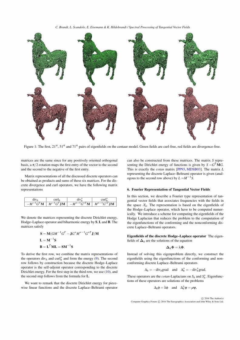
Figure 1: The first, 21st, 51st and 71st pairs of eigenfields on the centaur model. Green fields are curl-free, red fields are divergence-free.

matrices are the same since for any positively oriented orthogonalbasis, a π/2-rotation maps the first entry of the vector to the secondand the second to the negative of the first entry.

Matrix representations of all the discussed discrete operators canbe obtained as products and sums of these six matrices. For the dis-crete divergence and curl operators, we have the following matrixrepresentations

divh curlh div∗h curl∗h−M−1GT M M−1GT JM −M∗−1G∗T M M∗−1G∗T JM

We denote the matrices representing the discrete Dirichlet energy,Hodge–Laplace operator and biharmonic energy by S,L and B. Thematrices satisfy

S = M(GM−1GT −JG∗M∗−1G∗T J)M

L = M−1S

B = LT ML = SM−1S

To derive the first row, we combine the matrix representations ofthe operators divh and curl∗h and form the energy (9). The secondrow follows by construction because the discrete Hodge–Laplaceoperator is the self-adjoint operator corresponding to the discreteDirichlet energy. For the first step in the third row, we use (10), andthe second step follows from the formula for L.

We want to remark that the discrete Dirichlet energy for piece-wise linear functions and the discrete Laplace–Beltrami operator

can also be constructed from these matrices. The matrix S repre-senting the Dirichlet energy of functions is given by S =GT MG.This is exactly the cotan matrix [PP93, MDSB03]. The matrix Lrepresenting the discrete Laplace–Beltrami operator is given (anal-ogous to the second row above) by L =M−1S.

6. Fourier Representation of Tangential Vector Fields

In this section, we describe a Fourier type representation of tan-gential vector fields that associates frequencies with the fields inthe space Xh. The representation is based on the eigenfields ofthe Hodge–Laplace operator, which have to be computed numer-ically. We introduce a scheme for computing the eigenfields of theHodge Laplacian that reduces the problem to the computation ofthe eigenfunctions of the conforming and the nonconforming dis-crete Laplace–Beltrami operators.

Eigenfields of the discrete Hodge–Laplace operator The eigen-fields of ∆h are the solutions of the equation

∆hΦ = λΦ.

Instead of solving this eigenproblem directly, we construct theeigenfields using the eigenfunctions of the conforming and non-conforming discrete Laplace–Beltrami operators

∆h =−divhgrad and ∆∗h =−div∗h grad.

These operators are the cotan-Laplacians on Sh and S∗h . Eigenfunc-tions of these operators are solutions of the problems

∆hφ = λφ and ∆∗h ψ = µψ,



where φ ∈ Sh and ψ ∈ S∗h . The numerical treatment of the eigen-problem for the conforming operator is the basis for spectral geom-etry processing and is treated in detail in [VL08]. The nonconform-ing case can be treated in the same way, only the matrices M∗ andS∗ = G∗T MG∗ are used instead of M and S = GT MG.

The following Lemma summarizes the relation of the eigenfunc-tions of ∆h and ∆

∗h and the eigenfields of ∆h and is the basis of our

scheme for computing the eigenfields.

Lemma 1 The gradient of any eigenfunction of ∆h is an eigen-field of ∆h and the co-gradient of any eigenfunction of ∆

∗h is an

eigenfield of ∆h. The eigenvalues of an eigenfunction and the cor-responding eigenfield are the same.

Proof Let φ be an eigenfunction of ∆h with eigenvalue λ. Then,

∆hgrad φ =−grad divhgrad φ− J grad curl∗h grad φ

= grad ∆h φ = λgrad φ.

This proves the lemma for eigenfunctions of ∆h. The statementabout the co-gradients of eigenfunctions of ∆

∗h is proved in a similar

manner.

Fourier representation We denote the number of vertices, edgesand the genus of our mesh by nv, ne, and g. The following lemmashows that we can use Lemma 1 to construct an orthonormal basisof Xh.

Lemma 2 Let {φ0,φ1, ...,φnv−1} and {ψ0,ψ1, ...,ψne−1} beeigenbases of ∆h and ∆

∗h (where φ0 and ψ0 are the con-

stant functions), and let {Γ1,Γ2, ...,Γ2g} be an orthonor-mal basis of the subspace of harmonic fields Hh. Then, theset B = {Φ1,Φ2, ...,Φnv−1,Ψ1,Ψ2, ...,Ψne−1,Γ1,Γ2, ...,Γ2g},where Φi =

1‖gradφi‖L2

gradφi and Ψi =1

‖gradψi‖L2J gradψi, is an

orthonormal basis of the space Xh of piecewise constant tangentialvector fields.

Proof We first show that any pair of vector fields from B is orthog-onal. For i 6= j, we have⟨

gradφi,gradφ j⟩

L2 =⟨∆hφi,φ j

⟩L2 = λi

⟨φi,φ j

⟩L2 = 0,

which implies ⟨Φi,Φ j

⟩L2 = 0.

In a similar manner, we can show that any pair Ψi,Ψ j is orthonor-mal. The discrete Hodge decomposition (7) guarantees that anypair of vector fields with different letters is orthogonal, becausesuch fields are in different components of the Hodge decompo-sition. It remains to show that the number of vector fields in theset equals the dimension of the space Hh. The set B consistes of|B| = nv − 1 + ne − 1 + g vector fields. Using the Euler formulanv− ne + n f = 2− 2g, we get |B| = 2ne− n f . Since our mesh isa closed manifold, every edge is in two triangles, which means3n f = 2ne. Using this equation, we get |B| = 2n f , which is exactythe dimesion of Xh. We showed that B is an orthonormal set in Xhwith 2n f elements, which proves that B is an orthonormal basis ofXh.

As consequence of the lemma, we can represent any field v∈Xh

in the basis B

v =nv−1

∑i=1

αiΦi +ne−1

∑i=1

βiΨi +2g

∑i=1

γiΓi, (11)

where αi = 〈v,Φi〉L2 , βi = 〈v,Ψi〉L2 and γi = 〈v,Γi〉L2 . Since anybasis field is an eigenfield of the discrete Hodge–Laplace operator,we can associate a frequency, the square root of the eigenvalue, toevery basis field. Hence, this representation associates frequencieswith tangential vector fields. In this sense, (11) is a Fourier repre-sentation. In the following sections, we will show benefits of thisrepresentation for the applications.

In the continuous case, the eigenfunctions come in pairs. Forevery eigenfield Φ, the rotated field, J Φ, is also an eigenfield withthe same eigenvalue. Since we construct the basis as gradients andco-gradients of eigenfunction of the Laplace–Beltrami operator, wechoose in every eigenspace the basis such that every basis vector isin one component of the Hodge decomposition. As a result, theFourier representation refines the Hodge decomposition. Since inthe discrete case two different function space, Sh and S∗h , have to becombined, the symmetry is broken and “pairs” of eigenfields haveonly approximately the same eigenvalues. Figure 1 shows “pairs”of eigenfields of the discrete operator.

Computation of the eigenfields Our scheme for computing thelow-frequency eigenfields proceeds in three steps. The input is amaximum eigenvalue λmax (or alternatively the number of eigen-fields to be computed). The first step is to compute a basis of thespace of discrete harmonic fields (which along the way providesus with a basis of the cohomology of the surface). The space is2g-dimensional, where g is the genus of the surface. The idea isto project 2g random vector fields to the space of harmonic fields.These will span the space of harmonic fields (the probability thatthe random vectors or their projections are linearly dependent van-ishes). Finally, we orthonormalize these vectors. To project a vectorfield v into the space of harmonic fields, we remove the integrableand the co-integrable parts. The potentials of the integrable and theco-integrable part can be determined by solving the least squaresproblem

argminf∈Sh,g∈S∗h

‖v−grad f − J grad g‖2 .

Since the integrable and co-integrable parts are orthogonal, solv-ing this problem can be carried out in two steps: first computethe integrable part, then the co-integrable part. Both steps requiresolving a linear system where the matrices are the cotan matricesS = GT MG and S∗ = G∗T MG∗. The second step is to compute lin-early independent eigenfunctions φ of ∆h with eigenvalue smallerthan λmax. Since all eigenvalues are positive, we compute bands ofeigenfunctions with increasing eigenvalue starting with zero untilwe reach λmax. Then we compute the corresponding eigenfieldsΦ =grad φ and orthonormalize them. The third step is to computethe eigenfunctions ψ of ∆

∗h with eigenvalue smaller than λmax. As

before, we compute the corresponding eigenfields Ψ=J grad ψ andorthonormalize them. For the computation of the eigenfunctions of∆h and ∆

∗h , we follow [VL08].

The resulting eigenbasis refines the discrete Hodge decompo-sition. By construction each type of eigenfield belongs to one sub-



space ofXh. The fields Φ are in the integrable component, the fieldsΨ in the co-integrable component and the rest forms a basis of thespace of harmonic fields.

7. Tangential Vector Field Splines

Many classical splines can be characterized by variational princi-ples. Splines in tension are minimizers of a weighted sum of thebiharmonic and the Dirichlet energy subject to constraints (cubicsplines are the special case when the weight of the Dirichlet energyvanishes). Following the classical example, we define the tangen-tial vector field splines (TVFS) as minimizers of the weighted sumof the biharmonic and the Dirichlet energy

EB(v)+ωED(v) (12)

subject to linear equality constraints on the vectors of v and itsdivergence and curl. Vortices can be constructed by prescribingnon-zero curl, sinks and sources are created via positive or nega-tive divergence respectively. Alternatively, singularities can be con-structed by specifying a few vector constraints around their desiredlocations. We refer to the several images and the supplementaryvideo to see several examples of this type of topology control inaction. The biharmonic energy is needed to obtain smooth enoughvector fields that satisfy the hard constraints. The effect is shown inFigure 2.

We want to remark that the idea of defining tangential vectorfield splines as minimizers of (12) was introduced in [FSDH07] asan extension of their vector field design approach. However, theirapproach has two limitations: only soft constraints can be imposedand the resulting scheme is not fast enough to allow for interactiveediting.

Real-time computation The computation of a TVFS amounts tosolving a sparse quadratic problem with linear equality constraints.The challenge is to solve the problems at real-time rates to enablean interactive TVFS editor.

Directly solving the resulting linear systems to compute a TVFSis not an option since this can take several minutes. Directly re-using a sparse factorization is not possible, because the size ofthe matrix changes, whenever constraints are added or removed.A fast approximation algorithm can be established using the basisof eigenfields. We are using the property of the eigenbasis that in

Figure 2: The per-face Dirichlet energy of a tangential vector fieldspline from a single constraint on an irregular sphere is shown (red:high Dirichlet energy, green: low Dirichlet energy). On the left, weshow the minimizer of the Dirichlet energy only, without higherorder regularizer, on the right, we use the biharmonic energy (12)with low ω.

Figure 3: Real-time tangential vector field spline editing on the ar-madillo model (left, 331904 faces) and the resulting fur (right).

this basis the Dirichlet and the biharmonic energy are representedby diagonal matrices.

In a preprocess, we compute the d eigenfields with the smallesteigenvalue as described in Section 6. We assemble the vectors toform the columns of a matrix U ∈ R2n f×d . A tangent field in thed-dimensional subspace can be described by reduced coordinates,i.e., a vector v ∈ Rd . The matrix U transforms from reduced co-ordinates v to the full coordinates x = Uv ∈ R2n f . Since we areusing a basis of eigenfields, in the reduced coordinates the energiesare represented by diagonal matrices. The matrix Λ representingthe Dirichlet energy has the eigenvalues on the diagonal. Then, Λ2

represents the biharmonic energy and the resulting energy matrixD is

D = Λ2 +ωΛ.

We consider nc linear constraints, which in the unreduced coordi-nates have the form C̃x = c, where C̃ ∈ Rnc×2n f , c ∈ Rnc and x ∈R2n f . To constrain the divergence or curl of the field at a vertex oran edge, we copy the corresponding row from the divergence andcurl matrices (see Section 5) into C̃. The entry in the vector c speci-fies the value the divergence or curl assumes. Values at arbitrary lo-cations in a triangle can be specified using barycentric coordinates.In a similar manner, vectors in triangles can be prescribed. Oncethe matrix C̃ is constructed, we can obtain its reduced counterpartby matrix multiplication: C = C̃U. The matrix C ensures that thereduced solution exactly satisfies the constraints. The matrix is ofsmall size, C ∈ Rnc×d .

Now we describe how to efficiently solve the constrained linearsystem. We first consider the case of a surface of genus 0. In thiscase, the matrix D has full rank and since it is diagonal, it can beeasily inverted. Using Lagrange multipliers, represented by a vectorµ ∈ Rnc , the solution v of the constraint optimization problem iscomputed by solving the linear system

Dv−CT µ = 0

Cv = c

Instead of solving this system directly, we first transform it. Toeliminate v from the second equation, we multiply the first equa-



tion by CD−1 and subtract it from the second equation

Dv−CT µ = 0 (13)

CD−1CT µ = c (14)

To compute the solution v, we first solve (14) for µ and then (13)for v. To compute µ, we factor the matrix CD−1CT , which is avery small matrix of size nc×nc. A new factorization is computedwhenever the set of constraints changes, changing the value of theconstraints affects only the right-hand side of the equation. Solvingfor v is very fast since D is diagonal.

In the case, of a surface of genus g > 0, the matrix D has theharmonic fields in its kernel. The resulting system can be solvedby treating the harmonic part separately. The system can be re-arranged such that first the harmonic part and the Lagrange mul-tipliers are determined and then v is computed. An alternative is toslightly modify the system by setting the eigenvalues of the har-monic part to a small positive constant (e.g., a tenth of the lowestnon-zero eigenvalue).

Since we are restricting the computation to a subspace spannedby low-frequency fields, the algorithm computes a low-pass filteredTVFS. From a signal theoretic point of view, the TVFS are low-frequency fields by construction. Our computational scheme cuts-off the remaining high-frequencies of the field. In this sense, thereduced solution could even be the preferred solution. Using basesof 1-2k eigenfields, the reduced results are typically very close tothe TVFS.

8. Applications and Experiments

8.1. Computation of the eigenfields

Table 1 lists timings for the computation of the eigenfields of theHodge Laplacian. The column Bases setup contains the total timeto setup the conforming and nonconforming Laplace–Beltrami op-erator, computing their eigenfunctions and then computing theirgradients and co-gradients. To compute the low-frequency eigen-functions, we use the shift-and-invert Lanczos method. The im-plementation was done in Java with native calls to the MUMPSlibrary [ADKL01] for solving the sparse linear systems. The com-putation was performed on a Dell Precision M3800.

Figure 1 shows examples of low-frequency eigenfields. For eachintegrable field (green), the corresponding co-integrable field (red)is shown.

8.2. Spline editor for tangential fields

In Section 7, we described a system for modeling tangential vec-tor field splines in real-time, making use of our reduced basis. Weimplemented this system, using a dense Cholesky factorization andutilizing the GPU to quickly map from the reduced space to a fullfield representation. In total, we get real-time responses in an inter-active editing environment, where vector constraints can be spec-ified via click-and-drag and a globally optimal tangential field isinstantly updated. The method scales well with the sizes of themeshes and allows for real-time tangential vector field modelingon larger meshes: aside from mapping the reduced coordinates to

Figure 4: Comparison between editing using our tangential vectorfield spline editor as described in Section 7 (left) and using softconstrained vector field design (cf. [FSDH07]) (right). As can beseen, not all constraints on the right are satisfactorily obeyed.

the full representation (which can be done efficiently on the GPU),the size of the system to be solved is independent of the resolutionof the mesh.

In Table 1, 4th column, we list the resulting total time for gen-erating tangential vector field splines on various meshes from 30user defined constraints using a basis of 1000 eigenfields. We sepa-rately list the timings for setting-up and factorizing the system andthe timing for a solve (including the time for sending the reducedcoordinates to the GPU and there mapping them to the full repre-sentation). When a new constraint is added, both those steps haveto be executed, but if a constraint is just modified (e.g., changingthe direction of a vector constraint), only the solve time has to betaken into account, which is below 5ms even for our largest testmesh (the Armadillo mesh).

In Figure 4, top, we show a result of designing a vector fieldusing our spline editor. As can be seen, all constraints are exactlyobeyed but the overall field is still very smooth. In the supplemen-tary video, a real-time editing session can be seen. Another resultof TVFS editing on a high-resolution meshes can be seen in Fig-ures 3 and 5, where we effortlessly designed tangent vector fieldson meshes with 331k and 70k faces respectively.

8.3. Fur design

As an application of tangential vector field spline editing, we intro-duce a tool for fur design on surface meshes. A demonstration isshown in the supplementary video and results are shown in Figures5 and 3. The efficient and intuitive way to design smooth tangent

Model #faces Bases Spline Editing Reduced Soft Design Full Soft DesignName setup Setup \Solve Factor \Solve Factor \SolveHand 12184 23s 12ms \ 1ms 148ms \ 2.5ms 1.4s \ 16msRocker Arm 20088 43s 15ms \ 1ms 148ms \ 2.6ms 3.3s \ 28msBunny 69666 184s 18ms \ 2ms 155ms \ 2.4ms 22.7s \ 141msBumpy Torus 140240 395s 17ms \ 2ms 169ms \ 3.1ms 86.8s \ 379msArmadillo 331904 1246s 49ms \ 4ms 150ms \ 3.5ms 187.7s\ 818ms

Table 1: Timings for tangential vector field bases computation,solving the reduced tangential vector field spline system and solv-ing the reduced and full design system. In all three systems we useda second order energy term as an additional regularizer. In all exam-ples a basis size of 1000 was used (500 divergence free and 500 curlfree eigenfields of the Hodge–Laplace operator) and 30 constraintswere specified.



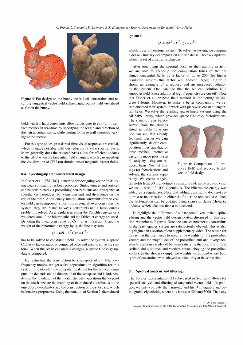
Figure 5: Fur design on the bunny mesh. Left: constraints and re-sulting tangential vector field spline, right: output field visualizedas fur on the bunny.

fields via few hard constraints allows a designer to edit fur on sur-face meshes in real-time by specifying the length and direction ofthe hair at certain spots, while aiming for an overall smoothly vary-ing hair direction.

For this type of design task real-time visual responses are crucial,which is made possible with our reduction via the spectral basis.More generally does the reduced basis allow for efficient updatesto the GPU when the tangential field changes, which can speed-upthe visualization of CPU-run simulations of tangential vector fields.

8.4. Speeding-up soft constrained design

In Fisher et al. [FSDH07], a method for designing vector fields us-ing weak constraints has been proposed. Sinks, sources and vorticescan be constructed via prescribing non-zero curl and divergence atspecific vertices/edges, but vanishing curl and divergence on therest of the mesh. Additionally, interpolation constraints for the vec-tor field can be imposed. Since this, in general, over-constrains thesystem, they are treated as weak constraints and a least-squaresproblem is solved. As a regularizer, either the Dirichlet energy or aweighted sum of the biharmonic and the Dirichlet energy are used.Denoting the linear constraints by C̃x = c, as in Section 7, and theweight of the biharmonic energy by ω, the linear system

(S+ωB+C̃T C̃)x = C̃T c

has to be solved to construct a field. To solve the system, a sparseCholesky factorization is computed once and used to solve the sys-tems. When the set of constraints changes, a sparse Cholesky up-date is computed.

By restricting the construction to a subspace of d =1-2k low-frequency modes, we get a fast approximation algorithm for thissystem. In particular, the computational cost for the reduced com-putation depends on the dimension of the subspace and is indepen-dent of the resolution of the mesh. The only operations that dependon the mesh size are the mapping of the reduced coordinates to theunreduced coordinates and the construction of the subspace, whichis done in a preprocess. Using the notation of Section 7, the reduced

system is

(Λ+ωΛ2 +CTC)v =CT c,

which is a d-dimensional system. To solve the system, we computea dense Cholesky decomposition and use dense Cholesky updates,when the set of constraints changes.

After employing the spectral basis to the resulting system,we are able to speed-up the computation times of the de-signed tangential fields by a factor of up to 200 (for higherresolution meshes this factor will become larger). Figure 6shows an example of a reduced and an unreduced solutionto the system. One can see that the reduced solution is asmoother field (since additional high frequencies are cut-off). Notethat Fisher et al. propose their method in the setting of dis-crete 1-forms. However, to make a better comparison, we re-implemented their system to work with piecewise constant tangen-tial fields. We solve the resulting sparse linear systems using theMUMPS library, which provides sparse Cholesky factorizations.

Figure 6: Comparison of unre-duced (left) and reduced (right)vector field design.

The speed-up can be ob-served from the timingslisted in Table 1, whereone can see, that alreadyfor small meshes we gainsignificantly shorter com-putation times, and that forlarge meshes, interactivedesign is made possible atall only by using our re-duced basis. We list tim-ings for factorizations andsolving the systems sepa-rately. We create tangen-tial fields from 30 user defined constraints and, in the reduced case,we use a basis of 1000 eigenfields. The biharmonic energy wasadded as a regularizer. Note that adding constraints does not re-quire a re-factorization in either the full or the reduced case, sincethe factorization can be updated using sparse or dense Choleskyupdates, which take less than a millisecond.

To highlight the difference of our tangential vector field splineediting and the vector field design system discussed in this sec-tion, we point to Figure 4. Here one can see how not all constraintsin the least squares system are satisfactorily obeyed. This is alsohighlighted in a section of our supplementary video. The reason forthis is that the user needs to specify the weights for the prescribedvectors and the magnitudes of the prescribed curl and divergence,which results in a trade-off between satisfying the locations of pre-scribed sinks, sources and vortices versus obeying the prescribedvectors. In the shown example, no weights were found where bothtypes of constraints were obeyed satisfactorily at the same time.

8.5. Spectral analysis and filtering

The Fourier representation (11) discussed in Section 6 allows forspectral analysis and filtering of tangential vector fields. In prac-tice, we only compute the harmonic and first k integrable and co-integrable eigenfields, where k is between 500 and 5000. Then any



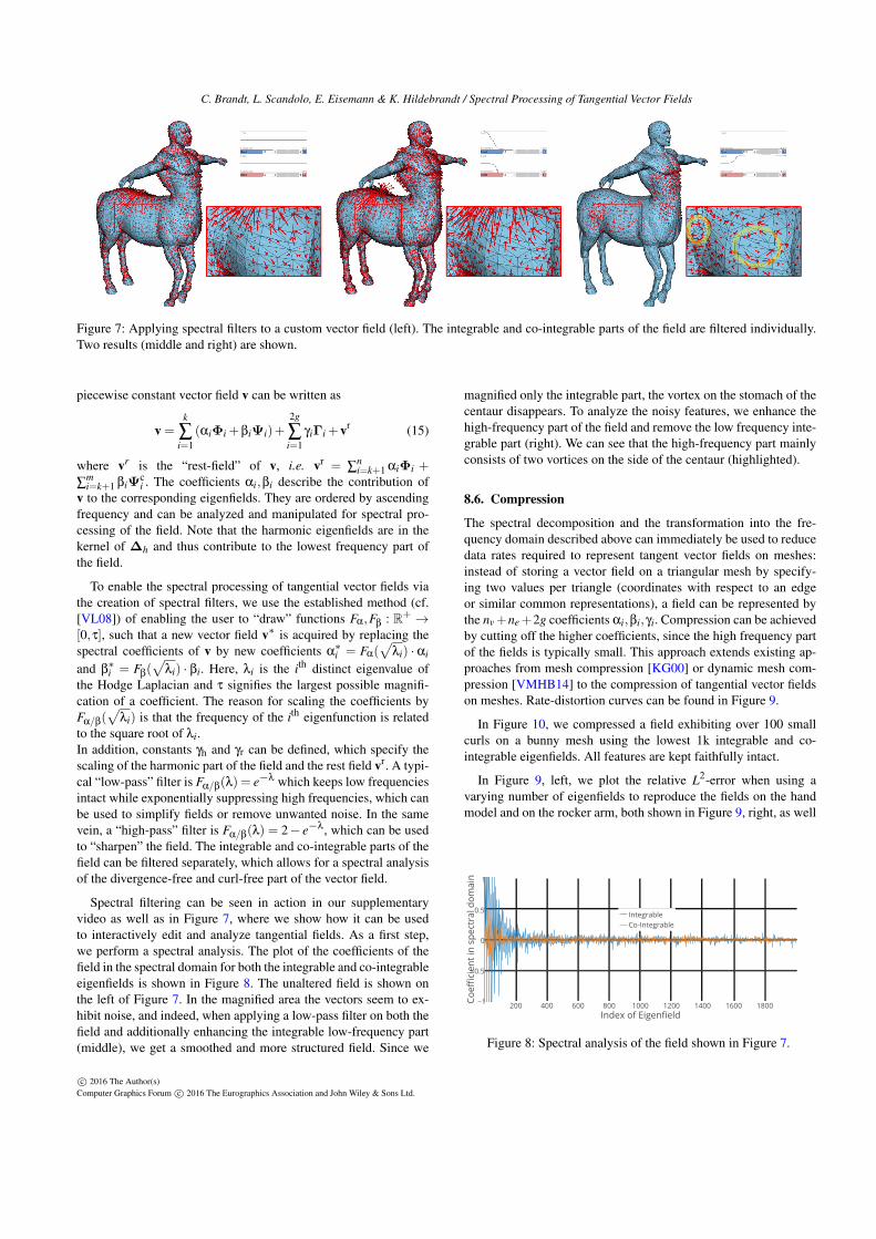
Figure 7: Applying spectral filters to a custom vector field (left). The integrable and co-integrable parts of the field are filtered individually.Two results (middle and right) are shown.

piecewise constant vector field v can be written as

v =k

∑i=1

(αiΦi +βiΨi)+2g

∑i=1

γiΓi +vr (15)

where vr is the “rest-field” of v, i.e. vr = ∑ni=k+1 αiΦi +

∑mi=k+1 βiΨ

ci . The coefficients αi,βi describe the contribution of

v to the corresponding eigenfields. They are ordered by ascendingfrequency and can be analyzed and manipulated for spectral pro-cessing of the field. Note that the harmonic eigenfields are in thekernel of ∆h and thus contribute to the lowest frequency part ofthe field.

To enable the spectral processing of tangential vector fields viathe creation of spectral filters, we use the established method (cf.[VL08]) of enabling the user to “draw” functions Fα,Fβ : R+ →[0,τ], such that a new vector field v∗ is acquired by replacing thespectral coefficients of v by new coefficients α

∗i = Fα(

√λi) · αi

and β∗i = Fβ(

√λi) · βi. Here, λi is the ith distinct eigenvalue of

the Hodge Laplacian and τ signifies the largest possible magnifi-cation of a coefficient. The reason for scaling the coefficients byFα/β(

√λi) is that the frequency of the ith eigenfunction is related

to the square root of λi.In addition, constants γh and γr can be defined, which specify thescaling of the harmonic part of the field and the rest field vr. A typi-cal “low-pass” filter is Fα/β(λ) = e−λ which keeps low frequenciesintact while exponentially suppressing high frequencies, which canbe used to simplify fields or remove unwanted noise. In the samevein, a “high-pass” filter is Fα/β(λ) = 2− e−λ, which can be usedto “sharpen” the field. The integrable and co-integrable parts of thefield can be filtered separately, which allows for a spectral analysisof the divergence-free and curl-free part of the vector field.

Spectral filtering can be seen in action in our supplementaryvideo as well as in Figure 7, where we show how it can be usedto interactively edit and analyze tangential fields. As a first step,we perform a spectral analysis. The plot of the coefficients of thefield in the spectral domain for both the integrable and co-integrableeigenfields is shown in Figure 8. The unaltered field is shown onthe left of Figure 7. In the magnified area the vectors seem to ex-hibit noise, and indeed, when applying a low-pass filter on both thefield and additionally enhancing the integrable low-frequency part(middle), we get a smoothed and more structured field. Since we

magnified only the integrable part, the vortex on the stomach of thecentaur disappears. To analyze the noisy features, we enhance thehigh-frequency part of the field and remove the low frequency inte-grable part (right). We can see that the high-frequency part mainlyconsists of two vortices on the side of the centaur (highlighted).

8.6. Compression

The spectral decomposition and the transformation into the fre-quency domain described above can immediately be used to reducedata rates required to represent tangent vector fields on meshes:instead of storing a vector field on a triangular mesh by specify-ing two values per triangle (coordinates with respect to an edgeor similar common representations), a field can be represented bythe nv+ne+2g coefficients αi,βi,γi. Compression can be achievedby cutting off the higher coefficients, since the high frequency partof the fields is typically small. This approach extends existing ap-proaches from mesh compression [KG00] or dynamic mesh com-pression [VMHB14] to the compression of tangential vector fieldson meshes. Rate-distortion curves can be found in Figure 9.

In Figure 10, we compressed a field exhibiting over 100 smallcurls on a bunny mesh using the lowest 1k integrable and co-integrable eigenfields. All features are kept faithfully intact.

In Figure 9, left, we plot the relative L2-error when using avarying number of eigenfields to reproduce the fields on the handmodel and on the rocker arm, both shown in Figure 9, right, as well

Figure 8: Spectral analysis of the field shown in Figure 7.



Figure 9: Rate distortion curves when compressing various customtangential vector fields on three different meshes.

as the field on the bunny shown in Figure 10. The plot is essentiallya rate-distortion curve, as the number k of pairs of eigenfields usedto compress the field directly relates to the data rate, namely thenumber of bits per vertex is 2 · 64 · k/n (where n is the number ofvertices) when using double precision for the coefficients. In caseof the tangential field on the bunny mesh, the error only slowlyconverges to 0, since the field contains a lot of high frequencyelements (of course, the error still reaches 0 as the number ofeigenfields reaches the number of vertices plus the number ofedges). This is visualized in Figure 10, right, where the part of thefield is shown which cannot be reproduced by the 1k lowest pairsof eigenfields (note that the LIC visualization shows the structureof the field, but does not reveal its magnitude). When creatingthe same plot for a more regular field, namely the ones shown inFigure 9, we can see that we are able to reach an almost losslesscompression by using the 2k lowest pairs of eigenfields. It is worthnoting that quite a large number of eigenfields is required to get alow L2-error, even for this fairly simple field, while a very smallnumber of eigenfields is required to get visually indistinguishableresults that preserve all the large features. The compression of thefield on the rocker arm yields the best results, where we get anessentially lossless compression for k = 1100, which correspondsto a compression rate of 36.52 when comparing to the usualrepresentation of two doubles per triangle.

Figure 10: A field exposing a lot of small features (left) and thecompressed version made from the 5from the 1000 lowest pairs(middle). In the last picture (right) we show the part of the origi-nal field that cannot be constructed from the 1000 lowest pairs ofeigenfields.

In Figure 11 we show a snapshot of a time-dependenttangent field on the bumpy torus (140240 faces),

Figure 11: Snapshot from theuncompressed (left) and com-pressed (right) time-dependenttangential vector field on thebumpy torus.

consisting of 500 fields,which amounts to a filesize of 560,96 Megabytewhen representing the vec-tors in each face by twosingle precision floatingpoint numbers (4 bytes).We compress the sequenceusing a basis of 500 eigen-fields which amounts toa file-size of exactly 1Megabyte. On average weget a relative L2-error of10 percent between com-pressed and uncompressedframes, however, as can beseen in the supplementaryvideo, where both time-series are shown next to each other, the twotime series are visually indistinguishable.

The timings for the compression are very low, once the eigen-fields have been computed, which only needs to be done once permesh (for timings see Table 1). Whenever a new field on the meshis to be compressed, all that needs to be done is to compute the L2-scalar products of the field with the 2 · k eigenfields (0.67 secondsfor the hand-mesh and k = 1000). Recovering the usual represen-tation of the vector simply requires a dense matrix vector productof the matrix containing the eigenfields as columns with the coeffi-cient vector (0.06 seconds for the hand-mesh and k = 1000, below1ms when done using the GPU).

9. Conclusion

We introduce a framework for spectral processing of tangentialvector fields using a Fourier-type representation of tangential vec-tor fields that associates frequencies with tangential vector fields.To formulate the framework for piecewise constant vector fieldson surface meshes, we introduce a discretization of the Hodge–Laplace operator. We demonstrate how techniques from spectralmesh processing can be transferred to tangential vector field pro-cessing using this framework. We show results for spectral filtering,analysis and compression. Moreover, we introduce a spline-like ed-itor for modeling tangential vector fields using interpolation con-straints. Based on the spectral representation, we propose a com-putational scheme that enables modeling of tangential vector fieldsplines in real-time.

Future work One direction of future work is to find more applica-tions of the Fourier representation of tangential vector fields, e.g.,by transferring techniques from spectral mesh processing to tan-gential vector field processing.

For applications, e.g., surface meshing, more general types offields (direction fields, RoSy fields,...) are considered. We areworking on establishing a Fourier-type representation for directionfields. This involves the construction of analog differential opera-tors and decompositions for these fields. In this paper, we are for-



mulating the Hodge Laplacian and Dirichlet energy in terms of theclassical operators grad, div and curl. This could be helpful sincerecent work is already addressing the construction of a curl opera-tor [DVPSH15] for direction fields to ensure integrability.

Acknowledgements

The idea of using a random projection algorithm for computingbases of the spaces harmonic vector fields originates from discus-sions with Max Wardetzky. We would like to thank Mirela Ben-Chen for inspiring discussions and the anonymous reviewers forhelpful comments and suggestions. This work was partially sup-ported by the EU project Harvest4D (FP7-323567) and the IntelVisual Computing Institute at Saarland University.

References[ADKL01] AMESTOY P. R., DUFF I. S., KOSTER J., L’EXCELLENT J.-

Y.: A fully asynchronous multifrontal solver using distributed dynamicscheduling. SIAM Journal on Matrix Analysis and Applications 23, 1(2001), 15–41. 9

[AF02] AGRICOLA I., FRIEDRICH T.: Global Analysis: DifferentialForms in Analysis, Geometry, and Physics. AMS, 2002. 5

[AFW06] ARNOLD D. N., FALK R. S., WINTHER R.: Finite elementexterior calculus, homological techniques, and applications. Acta nu-merica 15, 1 (2006). 3

[ASC11] AUBRY M., SCHLICKEWEI U., CREMERS D.: The wave ker-nel signature: A quantum mechanical approach to shape analysis. InICCV (2011), pp. 1626–1633. 2

[AVW∗15] AZENCOT O., VANTZOS O., WARDETZKY M., RUMPF M.,BEN-CHEN M.: Functional thin films on surfaces. In Symposium onComputer Animation (2015), pp. 137–146. 2

[AW11] ALEXA M., WARDETZKY M.: Discrete Laplacians on generalpolygonal meshes. ACM Trans. Graph. 30, 4 (2011), 102:1–102:10. 2

[AWO∗14] AZENCOT O., WEISSMANN S., OVSJANIKOV M.,WARDETZKY M., BEN-CHEN M.: Functional fluids on surfaces.In Computer Graphics Forum (2014), vol. 33. 2

[BKP∗10] BOTSCH M., KOBBELT L., PAULY M., ALLIEZ P., LEVY B.:Polygon Mesh Processing. AK Peters, 2010. 5

[BLP∗13] BOMMES D., LÉVY B., PIETRONI N., PUPPO E., SILVA C.,TARINI M., ZORIN D.: Quad-mesh generation and processing: A sur-vey. Comput. Graph. Forum 32, 6 (2013), 51–76. 3

[BNPB13] BHATIA H., NORGARD G., PASCUCCI V., BREMER P.-T.:The Helmholtz–Hodge decomposition—a survey. IEEE Transactions onVisualization and Computer Graphics 19, 8 (2013), 1386–1404. 3

[BZK09] BOMMES D., ZIMMER H., KOBBELT L.: Mixed-integer quad-rangulation. ACM Trans. Graph. 28, 3 (2009). 3

[CK14] CAMPEN M., KOBBELT L.: Quad layout embedding via alignedparameterization. Computer Graphics Forum 33, 8 (2014), 69–81. 3

[CYZL14] CHI M., YAO C., ZHANG E., LEE T.: Optical illusion shapetexturing using repeated asymmetric patterns. The Visual Computer 30,6-8 (2014). 2

[DBG∗06] DONG S., BREMER P.-T., GARLAND M., PASCUCCI V.,HART J. C.: Spectral surface quadrangulation. ACM Trans. Graph.25, 3 (2006), 1057–1066. 2

[dGDT15] DO GOES F., DESBRUN M., TONG Y.: Vector field pro-cessing on triangle meshes. In SIGGRAPH Asia 2015 Courses (2015),pp. 17:1–17:48. 2

[DHLM05] DESBRUN M., HIRANI A., LEOK M., MARSDEN J.: Dis-crete exterior calculus. preprint, arXiv:math.DG/0508341, 2005. 3

[DLL∗10] DEY T. K., LI K., LUO C., RANJAN P., SAFA I., WANGY.: Persistent heat signature for pose-oblivious matching of incompletemodels. Computer Graphics Forum 29, 5 (2010), 1545–1554. 2

[DRW10] DEY T. K., RANJAN P., WANG Y.: Convergence, stability, anddiscrete approximation of Laplace spectra. In Symp. Discrete Algorithms(2010), pp. 650–663. 2

[DVPSH14] DIAMANTI O., VAXMAN A., PANOZZO D., SORKINE-HORNUNG O.: Designing N-PolyVector fields with complex polyno-mials. Computer Graphics Forum 33, 5 (2014), 1–11. 3

[DVPSH15] DIAMANTI O., VAXMAN A., PANOZZO D., SORKINE-HORNUNG O.: Integrable PolyVector fields. ACM Trans. Graph. 34,4 (2015). 13

[DWLF12] DE WITT T., LESSIG C., FIUME E.: Fluid simulation usingLaplacian eigenfunctions. ACM Trans. Graph. 31, 1 (2012), 10:1–10:11.2

[ECBK14] EBKE H.-C., CAMPEN M., BOMMES D., KOBBELT L.:Level-of-detail quad meshing. ACM Trans. Graph. 33, 6 (2014), 184:1–184:11. 3

[FSDH07] FISHER M., SCHRÖDER P., DESBRUN M., HOPPE H.: De-sign of tangent vector fields. ACM Trans. Graph. 26, 3 (2007). 3, 8, 9,10

[GBAL09] GEBAL K., BÆRENTZEN J. A., AANÆS H., LARSEN R.:Shape analysis using the auto diffusion function. Computer GraphicsForum 28, 5 (2009), 1405–1413. 2

[HP11] HILDEBRANDT K., POLTHIER K.: On approximation of theLaplace–Beltrami operator and the Willmore energy of surfaces. Com-puter Graphics Forum 30, 5 (2011), 1513–1520. 2

[HPW06] HILDEBRANDT K., POLTHIER K., WARDETZKY M.: On theconvergence of metric and geometric properties of polyhedral surfaces.Geometricae Dedicata 123 (2006), 89–112. 2

[HSvTP10] HILDEBRANDT K., SCHULZ C., VON TYCOWICZ C.,POLTHIER K.: Eigenmodes of surface energies for shape analysis. InProceedings of Geometric Modeling and Processing (2010), pp. 296–314. 2

[HSvTP12] HILDEBRANDT K., SCHULZ C., VON TYCOWICZ C.,POLTHIER K.: Modal shape analysis beyond Laplacian. Computer AidedGeometric Design 29, 5 (2012), 204–218. 2

[HWAG09] HUANG Q., WICKE M., ADAMS B., GUIBAS L.: Shapedecomposition using modal analysis. Computer Graphics Forum 28, 2(2009), 407–416. 2

[HZ00] HERTZMANN A., ZORIN D.: Illustrating smooth surfaces. InProc. SIGGRAPH 2000 (2000). 2

[HZM∗08] HUANG J., ZHANG M., MA J., LIU X., KOBBELT L., BAOH.: Spectral quadrangulation with orientation and alignment control.ACM Trans. Graph. 27, 5 (2008), 1–9. 2

[IBB15] IARUSSI E., BOMMES D., BOUSSEAU A.: Bendfields: Regular-ized curvature fields from rough concept sketches. ACM Trans. Graph.34, 3 (2015). 2

[KCPS13] KNÖPPEL F., CRANE K., PINKALL U., SCHRÖDER P.: Glob-ally optimal direction fields. ACM Trans. Graph. 32, 4 (2013), 59:1–59:10. 3

[KCPS15] KNÖPPEL F., CRANE K., PINKALL U., SCHRÖDER P.: Stripepatterns on surfaces. ACM Trans. Graph. 34 (2015). 2

[KG00] KARNI Z., GOTSMAN C.: Spectral compression of mesh geom-etry. In ACM SIGGRAPH (2000), pp. 279–286. 2, 11

[KNP07] KÄLBERER F., NIESER M., POLTHIER K.: Quadcover - sur-face parameterization using branched coverings. Computer GraphicsForum 26, 3 (2007). 3

[LHJ∗14] LING R., HUANG J., JÜTTLER B., SUN F., BAO H., WANGW.: Spectral quadrangulation with feature curve alignment and elementsize control. ACM Trans. Graph. 34, 1 (2014), 11:1–11:11. 2



[LLW15] LI Y., LIU Y., WANG W.: Planar hexagonal meshing for archi-tecture. IEEE Trans. Vis. Comput. Graph. 21, 1 (2015). 3

[LLZ∗11] LI E., LÉVY B., ZHANG X., CHE W., DONG W., PAUL J.-C.: Meshless quadrangulation by global parameterization. Computers &Graphics (2011). 3

[LMH∗15] LIU B., MASON G., HODGSON J., TONG Y., DESBRUN M.:Model-reduced variational fluid simulation. ACM Trans. Graph. 34, 6(2015), 244:1–244:12. 2

[LZ09] LÉVY B., ZHANG H.: Spectral mesh processing. In ACM SIG-GRAPH ASIA Courses (2009), pp. 1–47. 2

[MDSB03] MEYER M., DESBRUN M., SCHRÖDER P., BARR A. H.:Discrete differential-geometry operators for triangulated 2-manifolds. InVisualization and Mathematics III. Springer, 2003, pp. 35–57. 2, 6

[MRMH12] MEHTA S. U., RAMAMOORTHI R., MEYER M., HERY C.:Analytic tangent irradiance environment maps for anisotropic surfaces.Computer Graphics Forum 31, 4 (2012). 2

[OBCS∗12] OVSJANIKOV M., BEN-CHEN M., SOLOMON J.,BUTSCHER A., GUIBAS L.: Functional maps: A flexible repre-sentation of maps between shapes. ACM Trans. Graph. 31, 4 (2012),30:1–30:11. 2

[OMMG10] OVSJANIKOV M., MÉRIGOT Q., MÉMOLI F., GUIBAS L.:One point isometric matching with the heat kernel. Computer GraphicsForum 29, 5 (2010), 1555–1564. 2

[OSG08] OVSJANIKOV M., SUN J., GUIBAS L.: Global intrinsic sym-metries of shapes. Computer Graphics Forum 27, 5 (2008), 1341–1348.2

[PLS∗15] PAN H., LIU Y., SHEFFER A., VINING N., LI C.-J., WANGW.: Flow aligned surfacing of curve networks. ACM Trans. Graph. 34,4 (2015). 2

[PP93] PINKALL U., POLTHIER K.: Computing discrete minimal sur-faces and their conjugates. Experimental Mathematics 2, 1 (1993), 15–36. 2, 5, 6

[PP00] POLTHIER K., PREUSS E.: Variational approach to vector fielddecomposition. In Proc. Eurographics Workshop on Scientific Visualiza-tion (2000), pp. 147–156. 3, 4

[PP03] POLTHIER K., PREUSS E.: Identifying vector field singularitiesusing a discrete Hodge decomposition. In Visualization and MathematicsIII (2003). 3, 4

[RGB∗14] RAYMOND B., GUENNEBAUD G., BARLA P., PACANOWSKIR., GRANIER X.: Optimizing brdf orientations for the manipulation ofanisotropic highlights. Comput. Graph. Forum 33, 2 (2014). 2

[RLL∗06] RAY N., LI W. C., LÉVY B., SHEFFER A., ALLIEZ P.: Pe-riodic global parameterization. ACM Trans. Graph. 25, 4 (2006), 1460–1485. 3

[ROA∗13] RUSTAMOV R. M., OVSJANIKOV M., AZENCOT O., BEN-CHEN M., CHAZAL F., GUIBAS L.: Map-based exploration of intrinsicshape differences and variability. ACM Trans. Graph. 32, 4 (2013), 72:1–72:12. 2

[Rus07] RUSTAMOV R. M.: Laplace–Beltrami eigenfunctions for de-formation invariant shape representation. In Symposium on GeometryProcessing (2007), pp. 225–233. 2

[RVLL08] RAY N., VALLET B., LI W. C., LÉVY B.: N-symmetry di-rection field design. ACM Trans. Graph. 27, 2 (2008). 3

[RWP05] REUTER M., WOLTER F.-E., PEINECKE N.: Laplace-spectraas fingerprints for shape matching. In Symposium on Solid and PhysicalModeling (2005), pp. 101–106. 2

[RWP06] REUTER M., WOLTER F.-E., PEINECKE N.: Laplace–Beltrami spectra as "Shape-DNA" of surfaces and solids. Computer-Aided Design 38, 4 (2006), 342–366. 2

[SBCBG11] SOLOMON J., BEN-CHEN M., BUTSCHER A., GUIBAS L.:Discovery of intrinsic primitives on triangle meshes. vol. 30, pp. 365–374. 2

[SHKvL09] SHARMA A., HORAUD R. P., KNOSSOW D., VON LA-VANTE E.: Mesh segmentation using Laplacian eigenvectors and Gaus-sian mixtures. In Manifold Learning and Its Applications (2009). 2

[SOG09] SUN J., OVSJANIKOV M., GUIBAS L. J.: A concise and prov-ably informative multi-scale signature based on heat diffusion. ComputerGraphics Forum 28, 5 (2009), 1383–1392. 2

[TLHD03] TONG Y., LOMBEYDA S., HIRANI A. N., DESBRUN M.:Discrete multiscale vector field decomposition. ACM Trans. Graph. 22,3 (2003), 445–452. 3, 4

[TPP∗11] TARINI M., PUPPO E., PANOZZO D., PIETRONI N.,CIGNONI P.: Simple quad domains for field aligned mesh parametriza-tion. ACM Trans. Graph. 30, 6 (2011). 3

[VCD∗16] VAXMAN A., CAMPEN M., DIAMANTI O., PANOZZO D.,BOMMES D., HILDEBRANDT K., BEN-CHEN M.: Directional FieldSynthesis, Design, and Processing. Computer Graphics Forum 35, 2(2016). 2

[VL08] VALLET B., LÉVY B.: Spectral geometry processing with man-ifold harmonics. Computer Graphics Forum (2008). 2, 7, 11

[VMHB14] VÁŠA L., MARRAS S., HORMANN K., BRUNNETT G.:Compressing dynamic meshes with geometric Laplacians. ComputerGraphics Forum 33, 2 (2014), 145–154. 2, 11

[War06] WARDETZKY M.: Discrete Differential Operators on Polyhe-dral Surfaces–Convergence and Approximation. PhD thesis, Freie Uni-versität Berlin, 2006. 3, 4

[War13] WARNER F. W.: Foundations of differentiable manifolds and Liegroups, vol. 94. Springer, 2013. 3

[WBH∗07] WARDETZKY M., BERGOU M., HARMON D., ZORIN D.,GRINSPUN E.: Discrete quadratic curvature energies. Comput. AidedGeom. Des. 24, 8-9 (2007). 4, 5

[WGH12] WAGNER C., GARTH C., HAGEN H.: Harmonic field analy-sis. In New Developments in the Visualization and Processing of TensorFields. Springer, 2012, pp. 363–379. 2

[WL01] WEI L.-Y., LEVOY M.: Texture synthesis over arbitrary mani-fold surfaces. In SIGGRAPH (2001). 2

[WMKG07] WARDETZKY M., MATHUR S., KÄLBERER F., GRINSPUNE.: Discrete Laplace operators: No free lunch. In Symposium on Geom-etry Processing (2007), pp. 33–37. 2

[YCLJ12] YAO C.-Y., CHI M.-T., LEE T.-Y., JU T.: Region-based linefield design using harmonic functions. IEEE Trans. Vis. Comput. Graph.18, 6 (2012). 2

[ZHT07] ZHANG E., HAYS J., TURK G.: Interactive tensor field designand visualization on surfaces. IEEE Trans. Vis. Comput. Graph. 13, 1(2007). 3

[ZMT06] ZHANG E., MISCHAIKOW K., TURK G.: Vector field designon surfaces. ACM Trans. Graph. 25, 4 (2006), 1294–1326. 3

[ZvKD10] ZHANG H., VAN KAICK O., DYER R.: Spectral mesh pro-cessing. Computer Graphics Forum 29, 6 (2010), 1865–1894. 2

[ZZCJ14] ZHUANG Y., ZOU M., CARR N., JU T.: Anisotropic geodesicsfor live-wire mesh segmentation. Comput. Graph. Forum 33, 7 (2014).2


Documents

Spectral Processing of Tangential Vector Fields · 2016-05-26 · Spectral mesh processing Within the last decade a large num-ber of methods for tasks in shape analysis and processing