Spectral Representation of Random Processes

Spectral Representation of Random Processes

Example: Represent u(t,x,Q) by!

u

K(t, x,Q) =KX

k=0

uk(t, x) k(Q)

where k(Q) are orthogonal polynomials.

Single Random Variable:!Let k(Q) be orthogonal with respect to ⇢Q(q) with 0(Q) = 1. Then

E[ 0(Q)] = 1

and!E[ i(Q) j(Q)] =

Z

� i(q) j(q)⇢Q(q)dq

= h i, ji⇢= �ij�i

Normalization factor:!

�i = E[ 2i (Q)] = h i, ii⇢

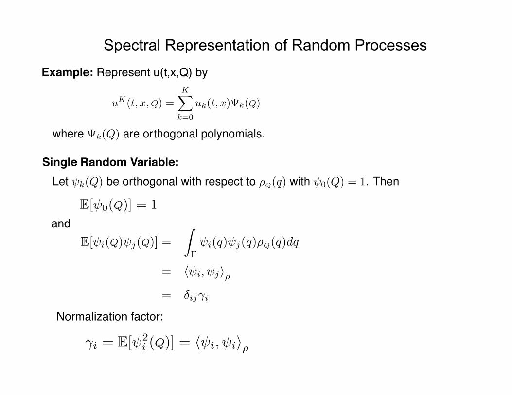
Random Process:!


E⇥u

K(t, x,Q)⇤= E

"KX

k=0

uk(t, x) k(Q)

#

= u0(t, x)E[ 0(Q)] +KX

k=1

uk(t, x)E[ k(Q)]

= u0(t, x)

var[uK(t, x,Q)] = Eh�u

K(t, x,Q)� E[uK(t, x,Q)]�2i

= E

2

4

KX

k=0

uk(t, x) k(Q)� u0(t, x)

!23

5

= E

2

4

KX

k=1

uk(t, x) k(Q)

!23

5

=KX

k=1

u

2k(t, x)�k

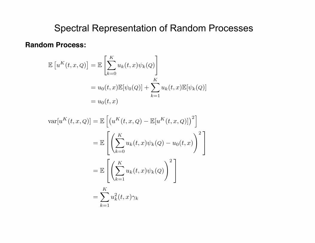
Hermite Polynomials:!


Q ⇠ N(0, 1)

Normalization factor:!

with the weight!

H0(Q) = 1 , H1(Q) = Q , H2(Q) = Q 2 � 1

H3(Q) = Q 3 � 3Q , H4(Q) = Q 4 � 6Q 2 + 3

⇢Q(q) =1p2⇡

e�q2/2

�i =

Z

R 2(q)⇢Q(q)dq = i!

Legendre Polynomials:!Q ⇠ U(�1, 1)

P0(Q) = 1 , P1(Q) = Q , P2(Q) =3

2Q 2 � 1

2

P3(Q) =5

2Q 3 � 3

2Q , P4(Q) =

35

8Q 4 � 15

4Q 2 +

3

8,

with the weight!

⇢Q(q) =1

2


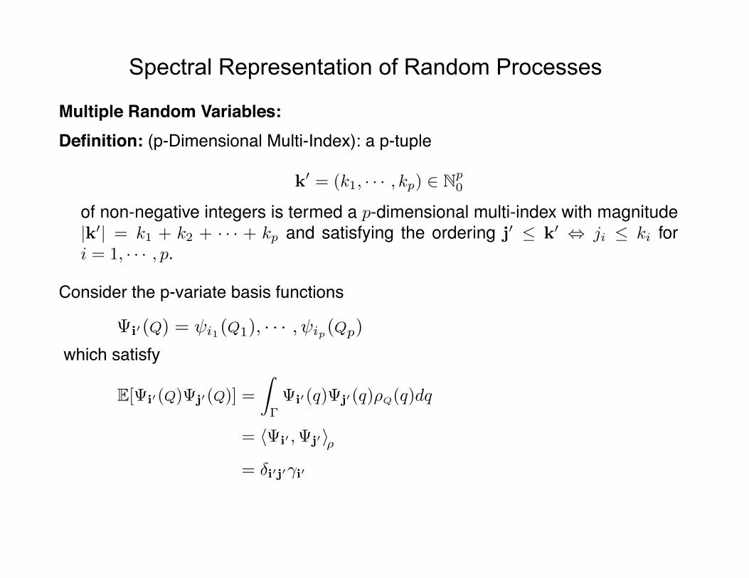
Multiple Random Variables:!Definition: (p-Dimensional Multi-Index): a p-tuple !

k0 = (k1, · · · , kp) 2 Np0

of non-negative integers is termed a p-dimensional multi-index with magnitude

|k0| = k1 + k2 + · · · + kp and satisfying the ordering j0 k0 , ji ki for

i = 1, · · · , p.

Consider the p-variate basis functions!

i0(Q) = i1(Q1), · · · , ip(Qp)

which satisfy !

E[ i0(Q) j0(Q)] =

Z

� i0(q) j0(q)⇢Q(q)dq

= h i0 , j0i⇢= �i0j0�i0


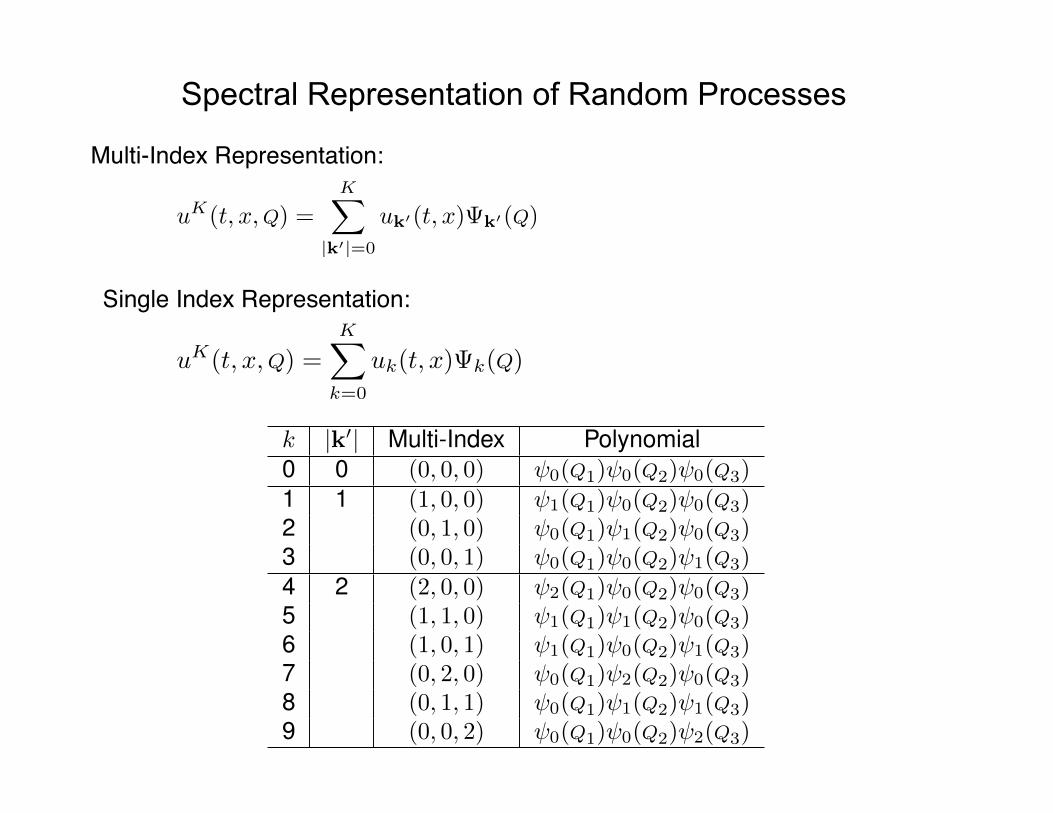
Multi-Index Representation:!

u

K(t, x,Q) =KX

|k0|=0

uk0(t, x) k0(Q)

Single Index Representation:!

u

K(t, x,Q) =KX

k=0

uk(t, x) k(Q)

k |k0| Multi-Index Polynomial

0 0 (0, 0, 0) 0(Q1) 0(Q2) 0(Q3)1 1 (1, 0, 0) 1(Q1) 0(Q2) 0(Q3)2 (0, 1, 0) 0(Q1) 1(Q2) 0(Q3)3 (0, 0, 1) 0(Q1) 0(Q2) 1(Q3)4 2 (2, 0, 0) 2(Q1) 0(Q2) 0(Q3)5 (1, 1, 0) 1(Q1) 1(Q2) 0(Q3)6 (1, 0, 1) 1(Q1) 0(Q2) 1(Q3)7 (0, 2, 0) 0(Q1) 2(Q2) 0(Q3)8 (0, 1, 1) 0(Q1) 1(Q2) 1(Q3)9 (0, 0, 2) 0(Q1) 0(Q2) 2(Q3)

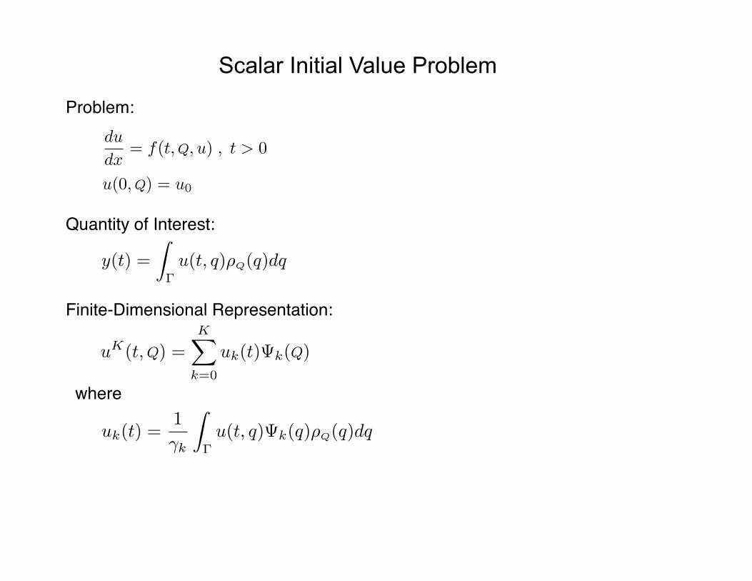
Scalar Initial Value Problem

Problem:!du

dx

= f(t,Q, u) , t > 0

u(0,Q) = u0

Quantity of Interest:!

y(t) =

Z

�u(t, q)⇢Q(q)dq

Finite-Dimensional Representation:!

uK(t,Q) =KX

k=0

uk(t) k(Q)

where!

uk(t) =1

�k

Z

�u(t, q) k(q)⇢Q(q)dq

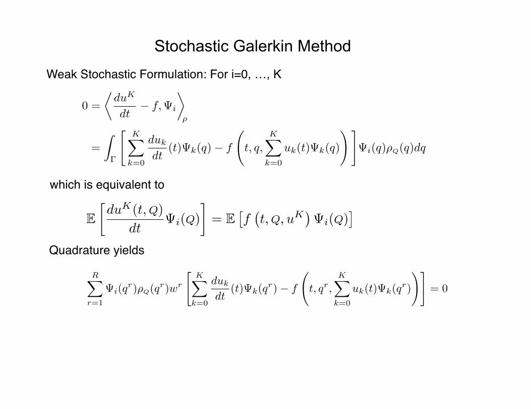
Stochastic Galerkin Method

Weak Stochastic Formulation: For i=0, …, K!

0 =

⌧duK

dt� f, i

�

⇢

=

Z

�

"KX

k=0

duk

dt(t) k(q)� f

t, q,

KX

k=0

uk(t) k(q)

!# i(q)⇢Q(q)dq

which is equivalent to!

EduK(t,Q)

dt i(Q)

�= E

⇥f�t,Q, uK

� i(Q)

⇤

Quadrature yields!

RX

r=1

i(qr)⇢Q(q

r)wr

"KX

k=0

duk

dt(t) k(q

r)� f

t, qr,

KX

k=0

uk(t) k(qr)

!#= 0


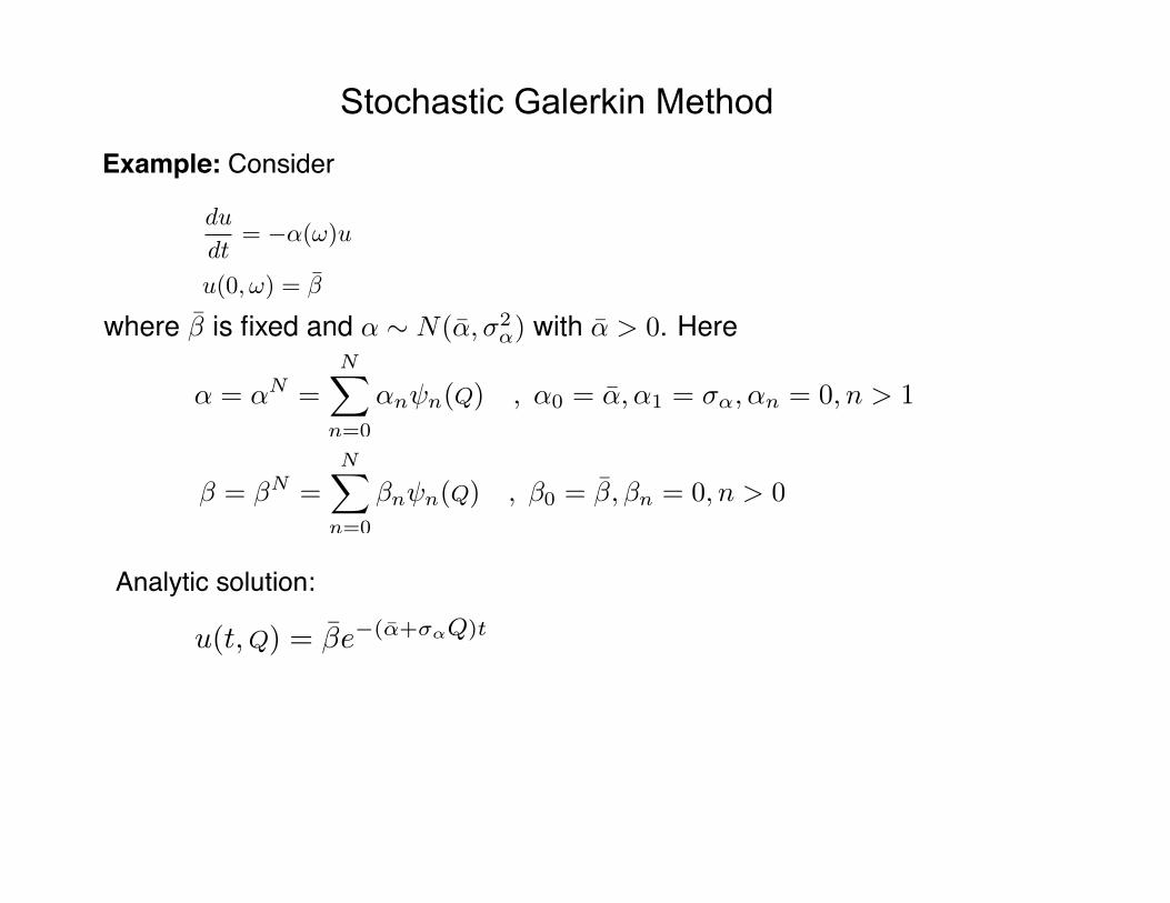
Example: Consider!

du

dt= �↵(!)u

u(0,!) = �

where � is fixed and ↵ ⇠ N(↵,�2↵) with ↵ > 0. Here

↵ = ↵N =NX

n=0

↵n n(Q) , ↵0 = ↵,↵1 = �↵,↵n = 0, n > 1

� = �N =NX

n=0

�n n(Q) , �0 = �,�n = 0, n > 0

Analytic solution:!

u(t,Q) = �e�(↵+�↵Q)t


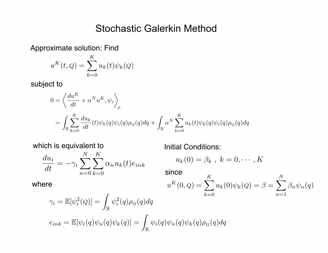
Approximate solution: Find!

uK(t,Q) =KX

k=0

uk(t) k(Q)

subject to!

0 =

⌧duK

dt+ ↵NuK , i

�

⇢

=

Z

R

KX

k=0

duk

dt(t) k(q) i(q)⇢Q(q)dq +

Z

R↵N

KX

k=0

uk(t) k(q) i(q)⇢Q(q)dq

which is equivalent to!dui

dt= ��i

NX

n=0

KX

k=0

↵nuk(t)eink

where!

�i = E[ 2i (Q)] =

Z

R 2i (q)⇢Q(q)dq

eink = E[ i(q) n(q) k(q)] =

Z

R i(q) n(q) k(q)⇢Q(q)dq

Initial Conditions:!uk(0) = �k , k = 0, · · · ,K

since!uK(0,Q) =

KX

k=0

uk(0) k(Q) = � =NX

n=1

�n n(q)

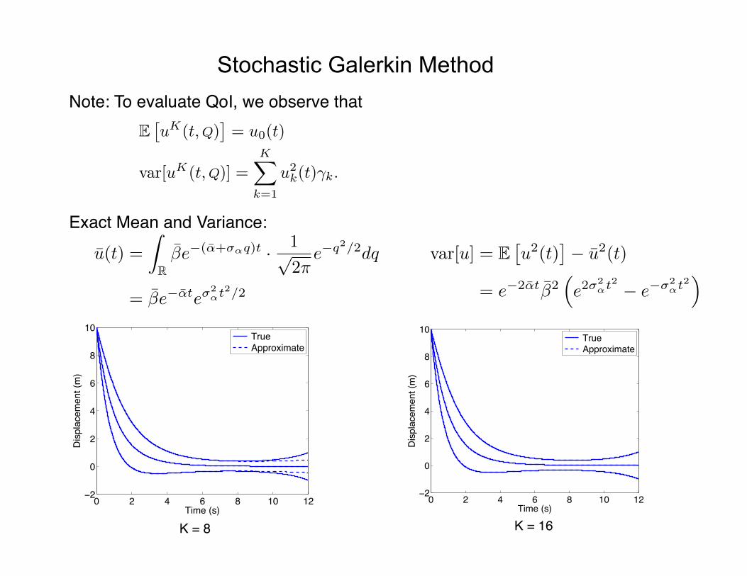
Stochastic Galerkin Method Note: To evaluate QoI, we observe that!

E⇥uK(t,Q)

⇤= u0(t)

var[uK(t,Q)] =KX

k=1

u2k(t)�k.

Exact Mean and Variance:!

u(t) =

Z

R�e�(↵+�↵q)t · 1p

2⇡e�q2/2dq

= �e�↵te�2↵t2/2

var[u] = E⇥u2(t)

⇤� u2(t)

= e�2↵t�2⇣e2�

2↵t2 � e��2

↵t2⌘

0 2 4 6 8 10 12−2

0

2

4

6

8

10

Time (s)

Dis

plac

emen

t (m

)

True Approximate

0 2 4 6 8 10 12−2

0

2

4

6

8

10

Time (s)

Dis

plac

emen

t (m

)

True Approximate

K = 8! K = 16!

Stochastic Galerkin Method Properties:!•  Accuracy is optimal in L2 sense.!

•  Disadvantages!§  Method is intrusive and hence difficult to implement with legacy

codes or codes for which only executable is available.!

§  Method requires densities with associated orthogonal polynomials. These can sometimes be constructed from empirical histograms.!

§  Method requires mutually independent parameters. !

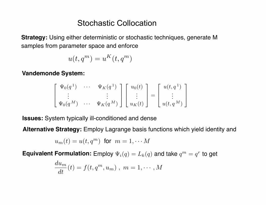
Stochastic Collocation

Strategy: Using either deterministic or stochastic techniques, generate M samples from parameter space and enforce!

u(t, qm) = uK(t, qm)

Vandemonde System:!2

64 0(q 1) · · · K(q 1)

......

0(qM ) · · · K(qM )

3

75

2

64u0(t)

...uK(t)

3

75 =

2

64u(t, q 1)

...u(t, qM )

3

75

Issues: System typically ill-conditioned and dense !

Alternative Strategy: Employ Lagrange basis functions which yield identity and !

um(t) = u(t, qm) for m = 1, · · ·M

Equivalent Formulation: !Employ i(q) = Lk(q) and take qm = qr to get

dum

dt(t) = f(t, qm, um) , m = 1, · · · ,M

Stochastic Collocation Properties:!•  Whereas motivated in the context of a Galerkin method, collocation is

based on interpolation theory.!•  Advantages!

§  Method is nonintrusive in the sense that once M collocation points are specified, one solves M deterministic problems using existing software.!

§  Method is applicable to general parameter distributions with correlated parameters.!

§  Algorithms available in Sandia Dakota package.!

•  Disadvantages!§  Evaluation of QoI typically requires sampling from joint distribution,

which may not be available.!

Discrete Projection Method

Problem:!du

dx

= f(t,Q, u) , t > 0

u(0,Q) = u0

Finite-Dimensional Representation:!

uK(t,Q) =KX

k=0

uk(t) k(Q)

where!

uk(t) =1

�k

Z

�u(t, q) k(q)⇢Q(q)dq

Discrete Projection (Pseudo-spectral):!

uk(t) =1

�k

RX

r=1

u(t, qr) k(qr)⇢Q(q

r)wr

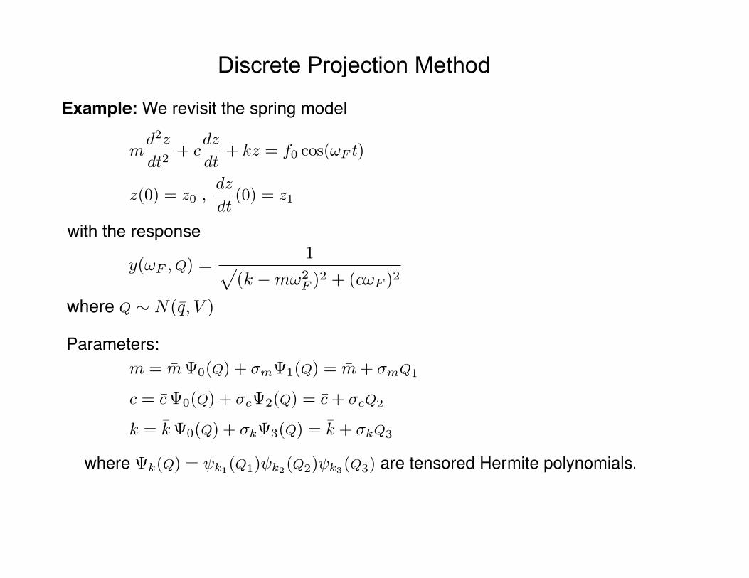
Discrete Projection Method

Example: We revisit the spring model!

md2z

dt2+ c

dz

dt+ kz = f0 cos(!F t)

z(0) = z0 ,dz

dt(0) = z1

with the response!

y(!F ,Q) =1p

(k �m!2F )

2 + (c!F )2

where Q ⇠ N(q, V )

Parameters:!m = m 0(Q) + �m 1(Q) = m+ �mQ1

c = c 0(Q) + �c 2(Q) = c+ �cQ2

k = k 0(Q) + �k 3(Q) = k + �kQ3

where k(Q) = k1(Q1) k2(Q2) k3(Q3) are tensored Hermite polynomials.

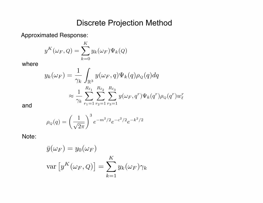
Discrete Projection Method Approximated Response:!

yK(!F ,Q) =KX

k=0

yk(!F ) k(Q)

where!

yk(!F ) =1

�k

Z

R3

y(!F , q) k(q)⇢Q(q)dq

⇡ 1

�k

R`1X

r1=1

R`2X

r2=1

R`3X

r3=1

y(!F , qr) k(q

r)⇢Q(qr)wr

`

and!

⇢Q(q) =

✓1p2⇡

◆3

e�m2/2e�c2/2e�k2/2

Note:!

y(!F ) = y0(!F )

var⇥yK(!F ,Q)

⇤=

KX

k=1

yk(!F )�k

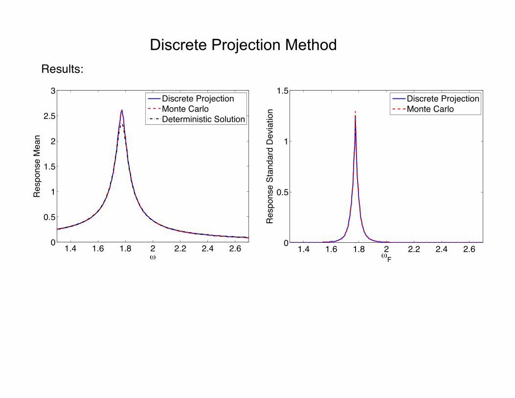
Discrete Projection Method Results:!

1.4 1.6 1.8 2 2.2 2.4 2.60

0.5

1

1.5

2

2.5

3

t

Res

pons

e M

ean

Discrete ProjectionMonte CarloDeterministic Solution

1.4 1.6 1.8 2 2.2 2.4 2.60

0.5

1

1.5

tFR

espo

nse

Stan

dard

Dev

iatio

n

Discrete ProjectionMonte Carlo

Discrete Projection Properties:!•  Advantages!

§  Like collocation, the method is nonintrusive and hence can be employed with post-processing to existing codes. The method is often referred to as nonintrusive PCE.!

§  Algorithms available in Sandia Dakota package.!

•  Disadvantages!§  Requires the construction of the joint density which often relies on

mutually independent parameters.!

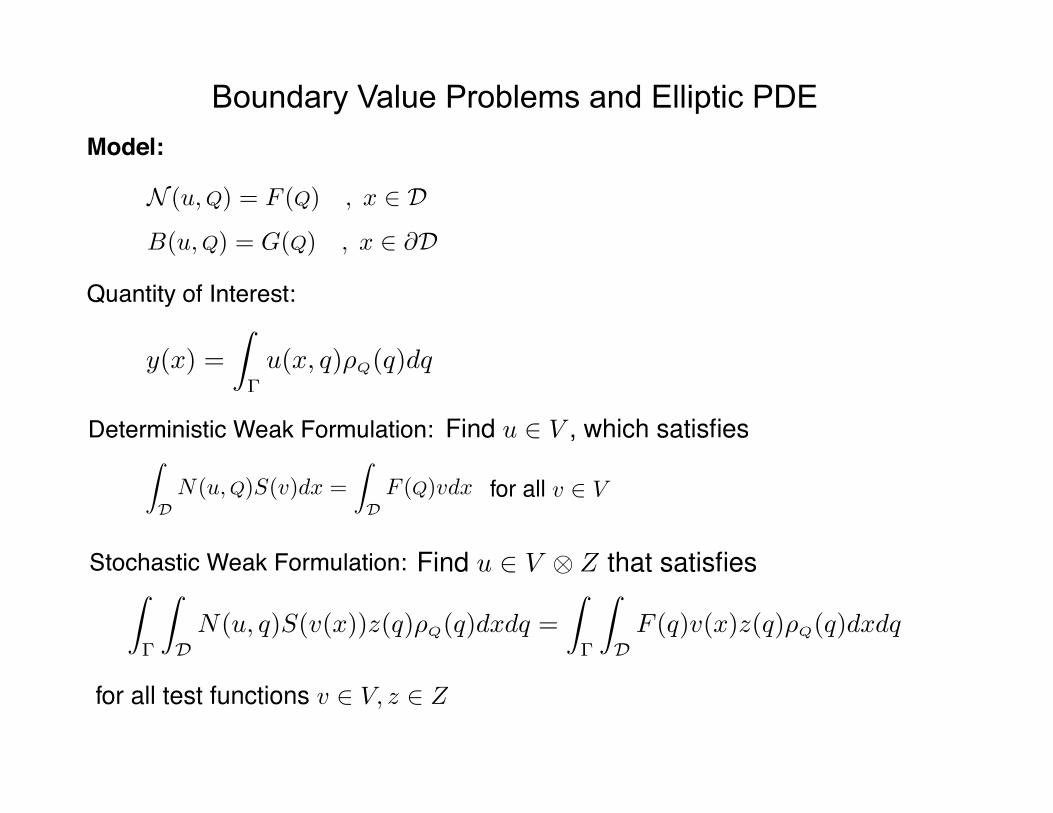
Boundary Value Problems and Elliptic PDE Model:!

N (u,Q) = F (Q) , x 2 D

B(u,Q) = G(Q) , x 2 @D


y(x) =

Z

�u(x, q)⇢Q(q)dq

Deterministic Weak Formulation:! Find u 2 V , which satisfiesZ

DN(u,Q)S(v)dx =

Z

DF (Q)vdx

for all v 2 V

Stochastic Weak Formulation:!Find u 2 V ⌦ Z that satisfiesZ

�

Z

DN(u, q)S(v(x))z(q)⇢Q(q)dxdq =

Z

�

Z

DF (q)v(x)z(q)⇢Q(q)dxdq

for all test functions v 2 V, z 2 Z

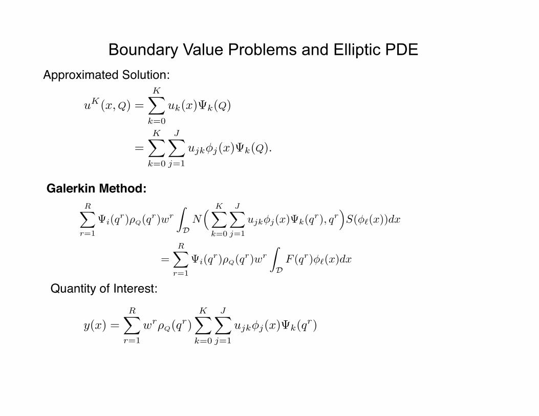
Boundary Value Problems and Elliptic PDE Approximated Solution:!

u

K(x,Q) =KX

k=0

uk(x) k(Q)

=KX

k=0

JX

j=1

ujk�j(x) k(Q).

Galerkin Method:!RX

r=1

i(qr)⇢Q(q

r)wr

Z

DN

⇣ KX

k=0

JX

j=1

ujk�j(x) k(qr), qr

⌘S(�`(x))dx

=RX

r=1

i(qr)⇢Q(q

r)wr

Z

DF (qr)�`(x)dx


y(x) =RX

r=1

w

r⇢Q(q

r)KX

k=0

JX

j=1

ujk�j(x) k(qr)

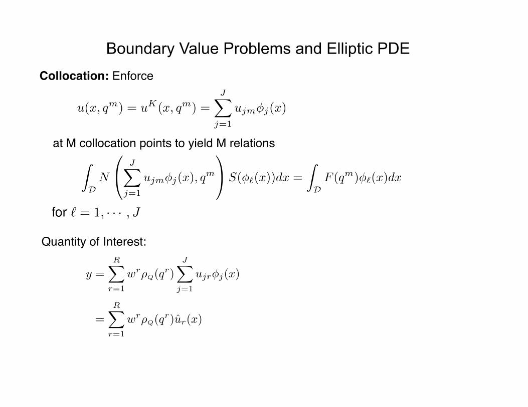
Boundary Value Problems and Elliptic PDE Collocation: Enforce!

u(x, qm) = u

K(x, qm) =JX

j=1

ujm�j(x)

at M collocation points to yield M relations!Z

DN

0

@JX

j=1

ujm�j(x), qm

1

AS(�`(x))dx =

Z

DF (qm)�`(x)dx

for ` = 1, · · · , J


y =RX

r=1

w

r⇢Q(q

r)JX

j=1

ujr�j(x)

=RX

r=1

w

r⇢Q(q

r)ur(x)

Documents

Spectral Representation of Random Processes