Embed Size (px)
Citation preview

1
Spectrum estimation using
Periodogram, Bartlett and Welch
Guido Schuster
Slides follow closely chapter 8 in the book „Statistical Digital Signal Processing and Modeling“ by Monson H. Hayes and most of the figures and formulas are taken from there
2
Introduction
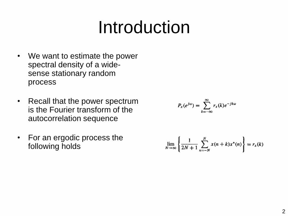
• We want to estimate the power spectral density of a wide-sense stationary random process
• Recall that the power spectrum is the Fourier transform of the autocorrelation sequence
• For an ergodic process the following holds
3
Introduction
• The main problem of power spectrum estimation is
– The data x(n) is always finite!
• Two basic approaches
– Nonparametric (Periodogram, Bartlett and Welch)
• These are the most common ones and will be presented in the next pages
– Parametric approaches
• not discussed here since they are less common
4
Nonparametric methods
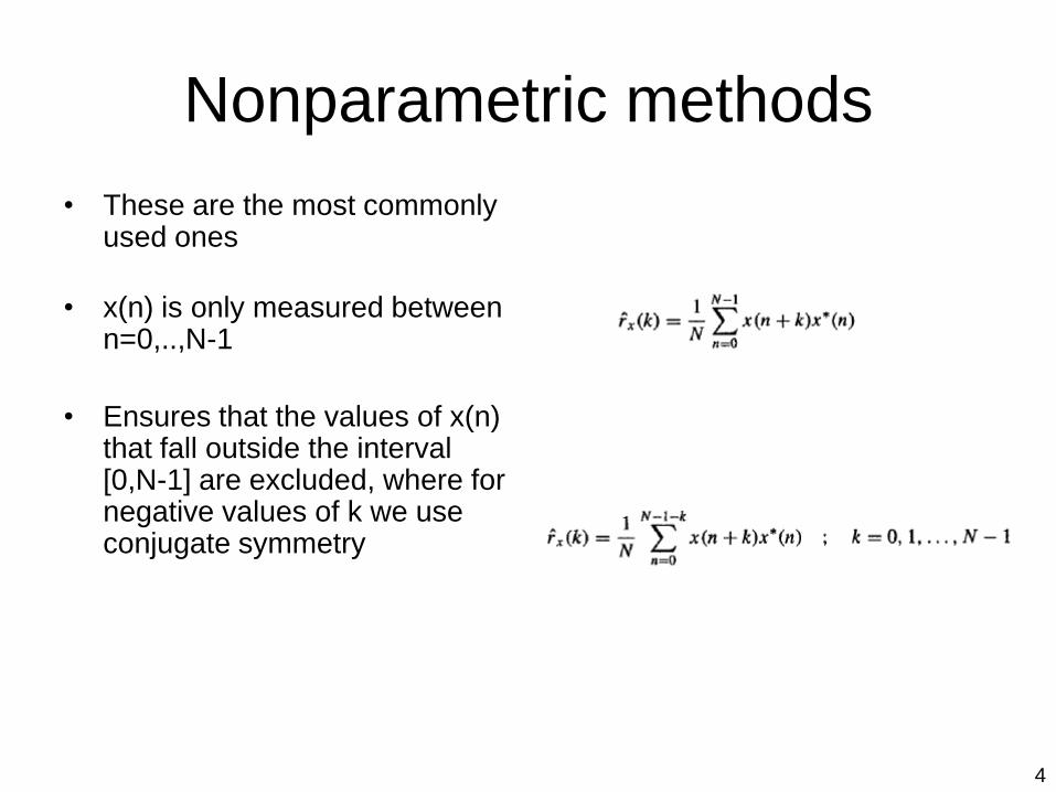
• These are the most commonly used ones
• x(n) is only measured between n=0,..,N-1
• Ensures that the values of x(n) that fall outside the interval [0,N-1] are excluded, where for negative values of k we use conjugate symmetry

5
Periodogram
• Taking the Fourier transform of this autocorrelation estimate results in an estimate of the power spectrum, known as the Periodogram
• This can also be directly expressed in terms of the data x(n) using the rectangular windowed function xN(n)
6
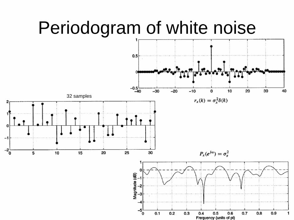
Periodogram of white noise
32 samples

7
Performance of the Periodogram
• If N goes to infinity, does the
Periodogram converge
towards the power spectrum in
the mean squared sense?
• Necessary conditions
– asymptotically unbiased:
– variance goes to zero:
• In other words, it must be a
consistent estimate of the
power spectrum

8
Recall: sample mean as estimator
• Assume that we measure an iid process x[n] with mean and
variance 2
• The sample mean is m=(x[0]+x[1]+x[2]+..+x[N-1])/N
• The sample mean is unbiased
E[m] =E[(x[0]+x[1]+x[2]+..+x[N-1])/N]
=(E[x[0]]+E[x[1]]+E[x[2]]+..+E[x[N-1]])/N
=N
=
• The variance of the sample mean is inversely proportional to the
number of samples
VAR[m] =VAR[(x[0]+x[1]+x[2]+..x[N-1])/N]=
=(VAR[x[0]]+VAR[x[1]]+VAR[x[2]]+..+VAR[x[N-1]])/N2
= N 2/N2
= 2/N
9
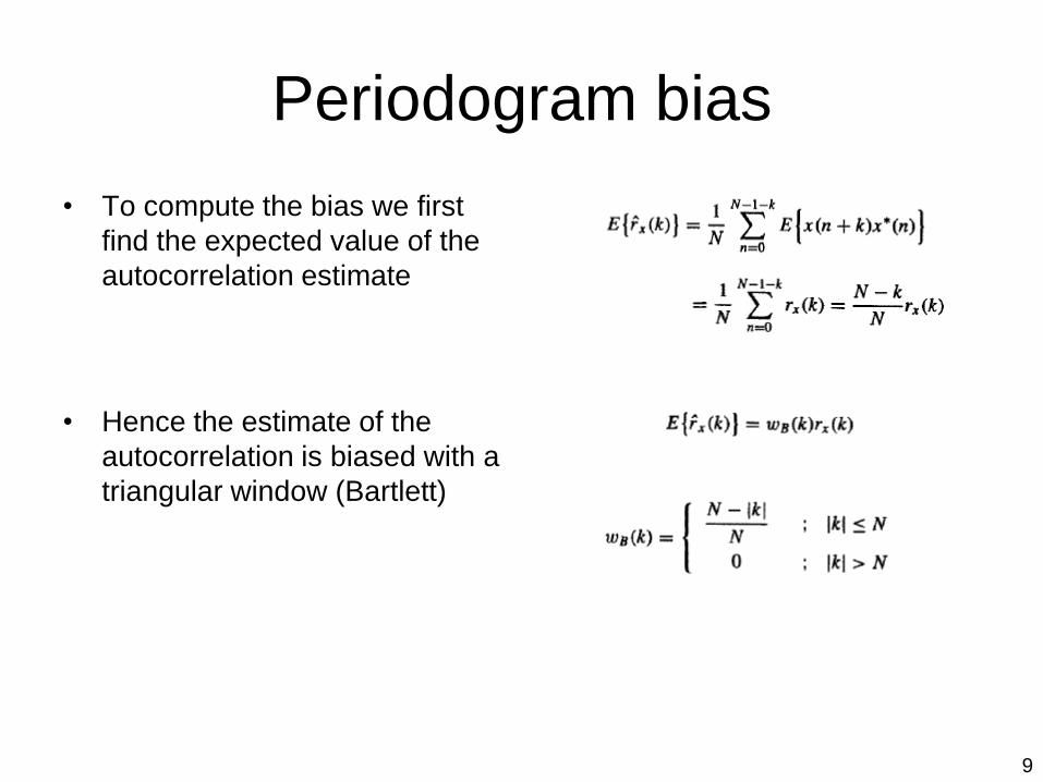
Periodogram bias
• To compute the bias we first
find the expected value of the
autocorrelation estimate
• Hence the estimate of the
autocorrelation is biased with a
triangular window (Bartlett)

10
Periodogram bias
• The expected value of the Periodogram can now be calculated:
• Thus the expected value of the Periodogram is the convolution of the power spectrum with the Fourier transform of a Bartlett window
11
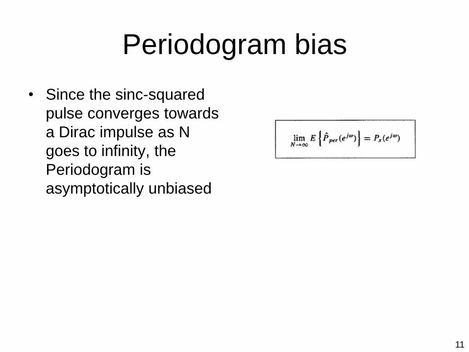
Periodogram bias
• Since the sinc-squared
pulse converges towards
a Dirac impulse as N
goes to infinity, the
Periodogram is
asymptotically unbiased
12
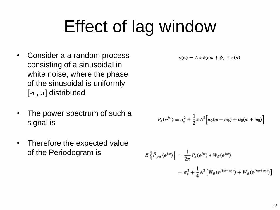
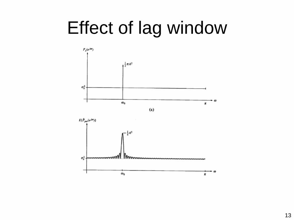
Effect of lag window
• Consider a a random process
consisting of a sinusoidal in
white noise, where the phase
of the sinusoidal is uniformly
[- , ] distributed
• The power spectrum of such a
signal is
• Therefore the expected value
of the Periodogram is
13
Effect of lag window
14
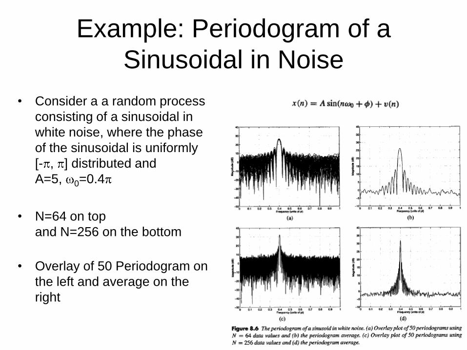
Example: Periodogram of a
Sinusoidal in Noise
• Consider a a random process
consisting of a sinusoidal in
white noise, where the phase
of the sinusoidal is uniformly
[- , ] distributed and
A=5, 0=0.4
• N=64 on top
and N=256 on the bottom
• Overlay of 50 Periodogram on
the left and average on the
right
15
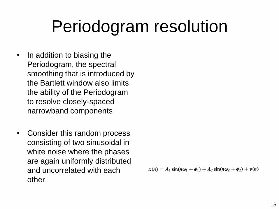
Periodogram resolution
• In addition to biasing the
Periodogram, the spectral
smoothing that is introduced by
the Bartlett window also limits
the ability of the Periodogram
to resolve closely-spaced
narrowband components
• Consider this random process
consisting of two sinusoidal in
white noise where the phases
are again uniformly distributed
and uncorrelated with each
other

16
Periodogram resolution
• The power spectrum of the
above random process is
• And the expected value of the
Periodogram is

17
Periodogram resolution
• Since the width of the main lobe increases as N decreases, for a given N there is a limit on how closely two sinusoidal may be located before they can no longer be resolved
• This is usually defined as the bandwidth of the window at its half power points (-6dB), which is for the Bartlett window at 0.89*2 /N
• This is just a rule of thumb!
18
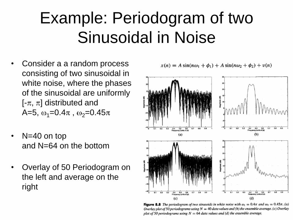
Example: Periodogram of two
Sinusoidal in Noise
• Consider a a random process
consisting of two sinusoidal in
white noise, where the phases
of the sinusoidal are uniformly
[- , ] distributed and
A=5, 1=0.4 , 2=0.45
• N=40 on top
and N=64 on the bottom
• Overlay of 50 Periodogram on
the left and average on the
right

19
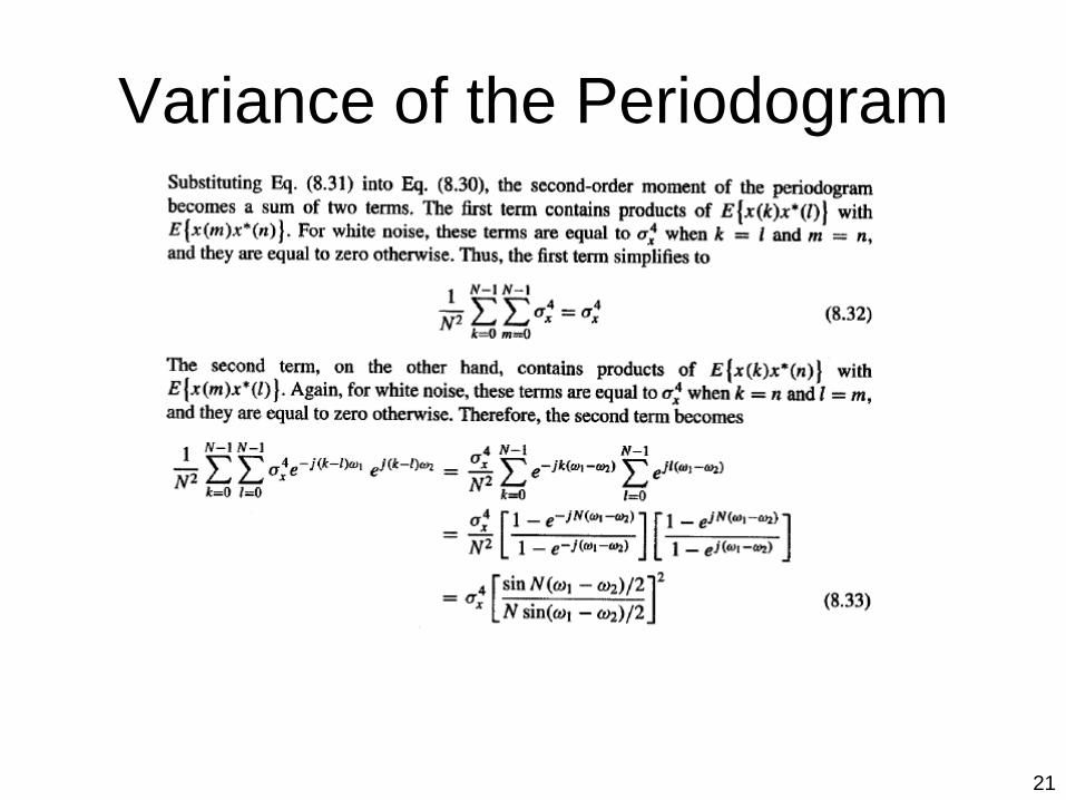
Variance of the Periodogram
• The Periodogram is an asymptotically unbiased estimate of the power spectrum
• To be a consistent estimate, it is necessary that the variance goes to zero as N goes to infinity
• This is however hard to show in general and hence we focus on a white Gaussian noise, which is still hard, but can be done

20
Variance of the Periodogram
21
Variance of the Periodogram

22
Variance of the Periodogram

23
Example: Periodogram of
white Gaussian noise• For a white Gaussian noise
with variance 1, the following
holds
• The expected value of the
Periodogram is
• Which results in
• And the variance is
• Which results in
24
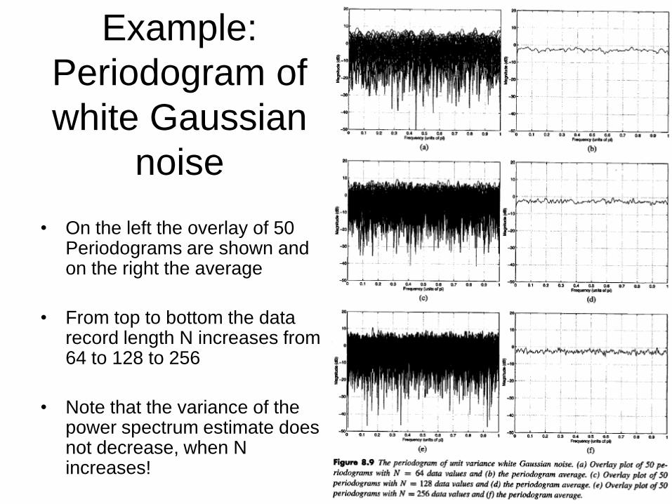
Example:
Periodogram of
white Gaussian
noise
• On the left the overlay of 50 Periodograms are shown and on the right the average
• From top to bottom the data record length N increases from 64 to 128 to 256
• Note that the variance of the power spectrum estimate does not decrease, when N increases!

25
So what if the process is not white
and/or not Gaussian?• Interpret the process as filtered
white noise v(n) with unit variance
• The white noise process and the colored noise process have the following Periodograms
• Although xN(n) is NOT equal to the convolution of vN(n) and h(n), if N is large compared to the length of h(n) then the transient effects are small
26
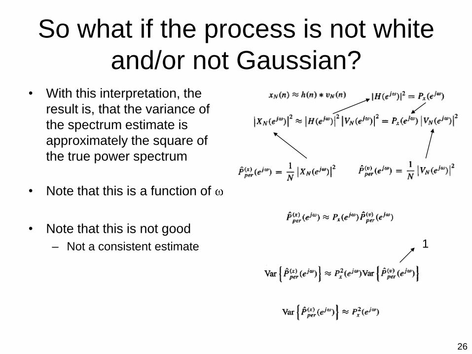
So what if the process is not white
and/or not Gaussian?• With this interpretation, the
result is, that the variance of
the spectrum estimate is
approximately the square of
the true power spectrum
• Note that this is a function of
• Note that this is not good
– Not a consistent estimate 1
27
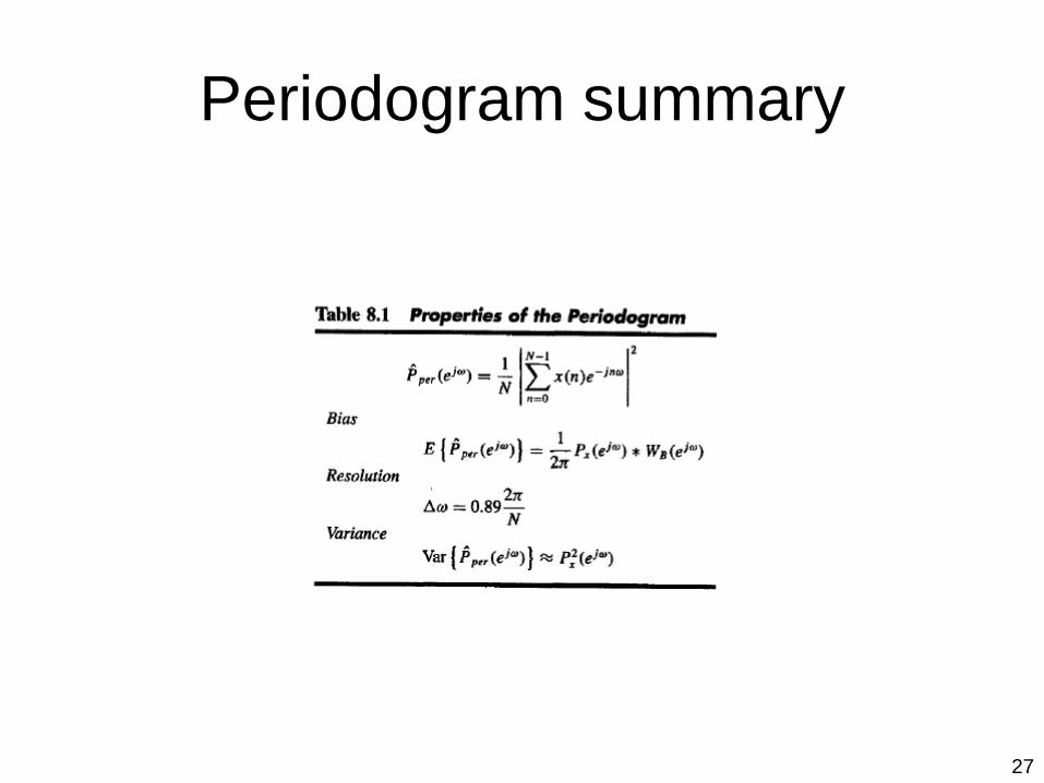
Periodogram summary

28
The modified Periodogram
• What happens when another
window (instead of the
rectangular window) is used?
• The window shows itself in the
Bias, but not directly but as a
convolution with itself

29
The modified Periodogram
• With the change of variables
k=n-m this becomes
• Where wB(k) is a Bartlett
window
• Hence in the frequency
domain, this becomes

30
The modified Periodogram
• Smoothing is determined by the window that is applied to the data
• While the rectangular window as the smallest main lobe of all
windows, its sidelobes fall off rather slowly
Hamming data windowRectangular data window

31
The modified Periodogram
• Nothing is free. As you notice, the Hamming window has a wider main lobe
• The Periodogram of a process that is windowed with a general window is called modified Periodogram
• N is the length of the window and U is a constant that is needed so that the modified Periodogram is asymptotically unbiased
32
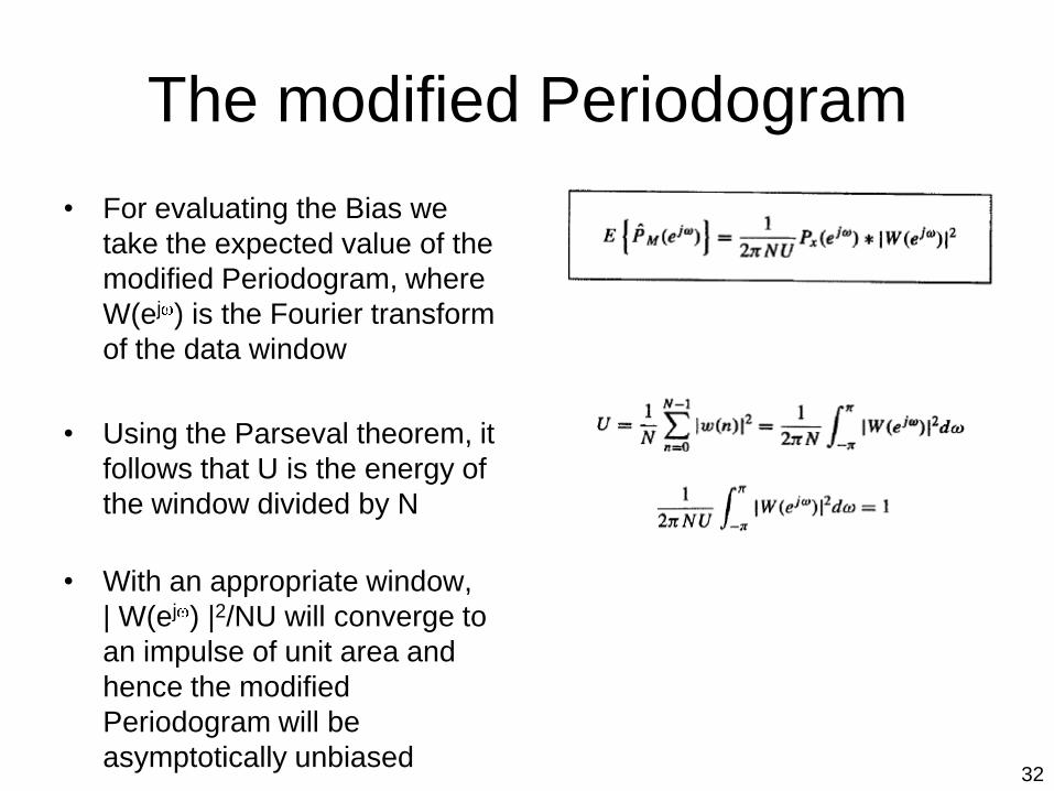
The modified Periodogram
• For evaluating the Bias we
take the expected value of the
modified Periodogram, where
W(ej ) is the Fourier transform
of the data window
• Using the Parseval theorem, it
follows that U is the energy of
the window divided by N
• With an appropriate window,
| W(ej ) |2/NU will converge to
an impulse of unit area and
hence the modified
Periodogram will be
asymptotically unbiased

33
Variance of the modified
Periodogram• Since the modified
Periodogram is simply the
Periodogram of a windowed
data sequence, not much
changes
• Hence the estimate is still not
consistent
• Main advantage is that the
window allows a tradeoff
between spectral resolution
(main lobe width) and spectral
masking (sidelobe amplitude)

34
Resolution versus masking of the
modified Periodogram• The resolution of the modified
Periodogram defined to be the
3dB bandwidth of the data
window
• Note that when we used the
Bartlett lag window before, the
resolution was defined as the
6dB bandwidth. This is
consistent with the above
definition, since the 3dB points
of the data window transform
into 6dB points in the
Periodogram

35
Modified periodogram summary
36
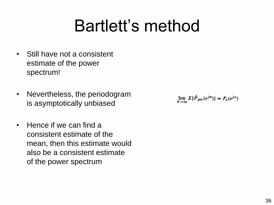
Bartlett’s method
• Still have not a consistent
estimate of the power
spectrum!
• Nevertheless, the periodogram
is asymptotically unbiased
• Hence if we can find a
consistent estimate of the
mean, then this estimate would
also be a consistent estimate
of the power spectrum

37
Bartlett’s method
• Averaging (sampe mean) a set of uncorrelated measurements of a
random variable results in a consistent estimate of its mean
• In other words: Variance of the sample mean is inversely
proportional to the number of measurements
• Hence this should also work here, by averaging Periodograms

38
Bartlett’s method
• Averaging these Periodograms
• This results in an asymptotically
unbiased estimate of the power
spectrum
• Since we assume that the
realizations are uncorrelated, it
follows, that the variance is
inversely proportional to the number
of measurements K
• Hence this is a consistent estimate
of the power spectrum, if L and K go
to infinity
39
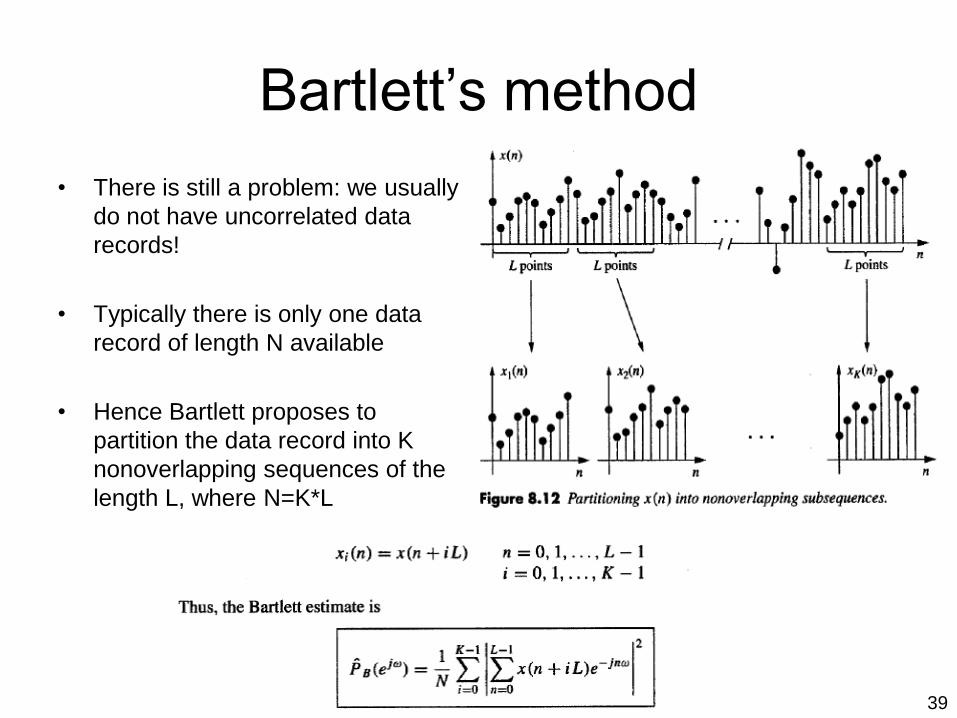
Bartlett’s method
• There is still a problem: we usually
do not have uncorrelated data
records!
• Typically there is only one data
record of length N available
• Hence Bartlett proposes to
partition the data record into K
nonoverlapping sequences of the
length L, where N=K*L

40
Bartlett’s method
• Each expected value of the
periodogram of the subsequences
are identical hence the process of
averaging subsequences
Periodograms results in the same
average value => asymptotically
unbiased
• Note that the data length used for
the Periodograms are now L and
not N anymore, the spectral
resolution becomes worse (this is
the price we are paying)
41
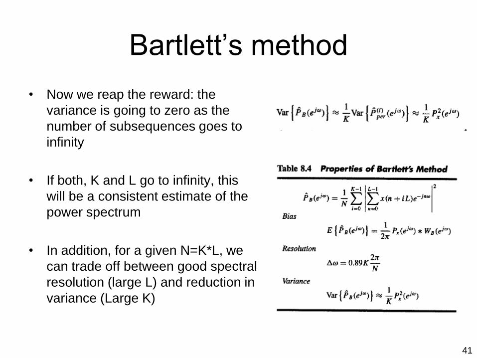
Bartlett’s method
• Now we reap the reward: the
variance is going to zero as the
number of subsequences goes to
infinity
• If both, K and L go to infinity, this
will be a consistent estimate of the
power spectrum
• In addition, for a given N=K*L, we
can trade off between good spectral
resolution (large L) and reduction in
variance (Large K)

42
Bartlett’s method:
White noise• a) Periodogram with N=512
• b) Ensemble average
• c) Overlay of 50 Bartlett
estimates with K=4 and L=128
• d) Ensemble average
• e) Overlay of 50 Bartlett
estimates with K=8 and L=64
• f) Ensemble average
Ensemble AverageOverlay of 50 estimates

43
Bartlett’s method: Two sinusoidal in
white noise• a) Periodogram with N=512
• b) Ensemble average
• c) Overlay of 50 Bartlett estimates with K=4 and L=128
• d) Ensemble average
• e) Overlay of 50 Bartlett estimates with K=8 and L=64
• f) Ensemble average
Note how larger K results in shorter L and hence in less spectral resolution

44
Welch’s method
• Two modifications to Bartlett’s
method
– 1) the subsequences are allowed to
overlap
– 2) instead of Periodograms,
modified Periodograms are
averaged
• Assuming that successive
sequences are offset by D points
and that each sequence is L points
long, then the ith sequence is
• Thus the overlap is L-D points and if
K sequences cover the entire N
data points then
45
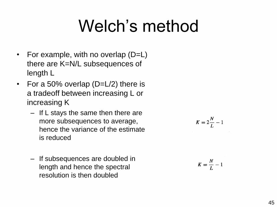
Welch’s method
• For example, with no overlap (D=L)
there are K=N/L subsequences of
length L
• For a 50% overlap (D=L/2) there is
a tradeoff between increasing L or
increasing K
– If L stays the same then there are
more subsequences to average,
hence the variance of the estimate
is reduced
– If subsequences are doubled in
length and hence the spectral
resolution is then doubled

46
Performance of Welch’s method
• Welch’s method can be written in
terms of the data record as follows
• Or in terms of modified
Periodograms
• Hence the expected value of
Welch’s estimate is
• Where W(ej ) is the Fourier
transform of the L-point data
window w(n)

47
Performance of Welch’s method
• Welch’s method is asymptotically
unbiased estimate of the power
spectrum
• The variance is much harder to
compute, since the overlap results
in a correlation
• Nevertheless for an overlap of 50%
and a Bartlett window it has been
shown that
• Recall Bartlett’s Method results in

48
Performance of Welch’s method
• For a fixed number of data N, with
50% overlap, twice as many
subsequences can be averaged,
hence expressing the variance in
terms of L and N we have
• Since N/L is the number of
subsequences K used in Bartlett’s
method it follows
• In other words, and not surprising,
with 50% overlap (and Bartlett
window), the variance of Welch’s
method is about half that of
Bartlett’s method

49
Welch’s method summary
50
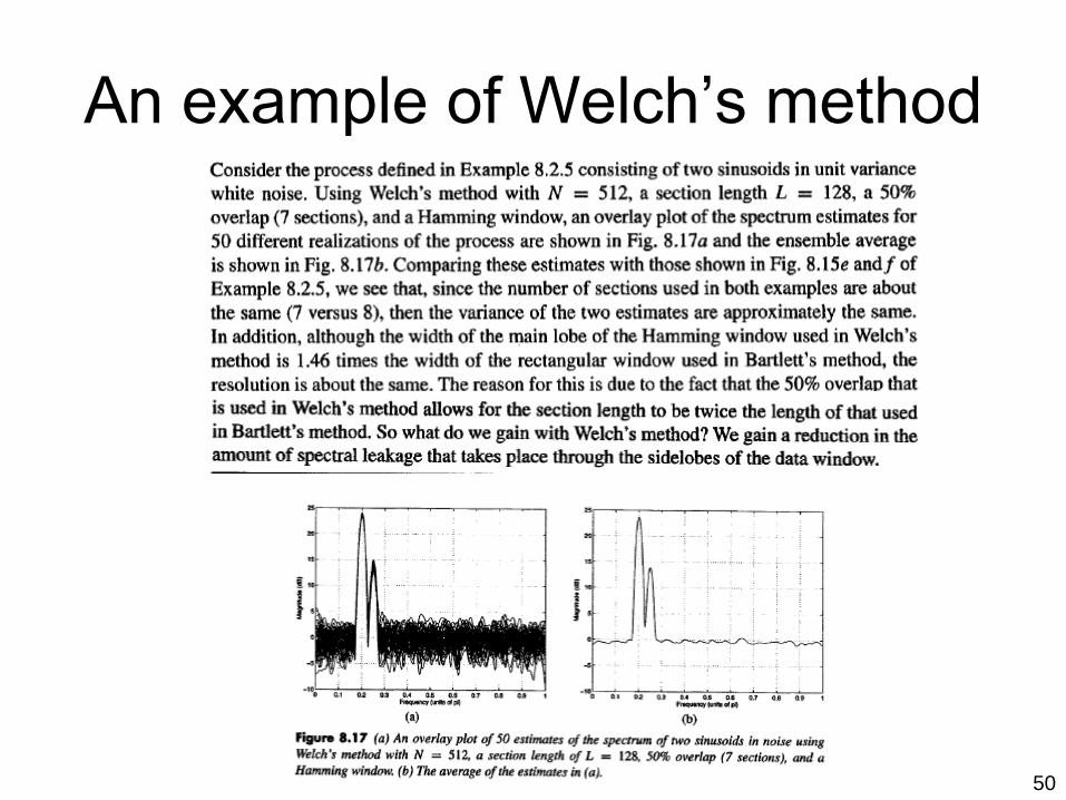
An example of Welch’s method

51
Exercises
52
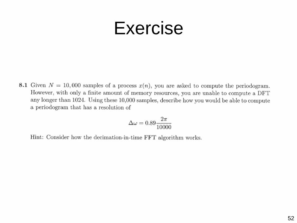
Exercise
53
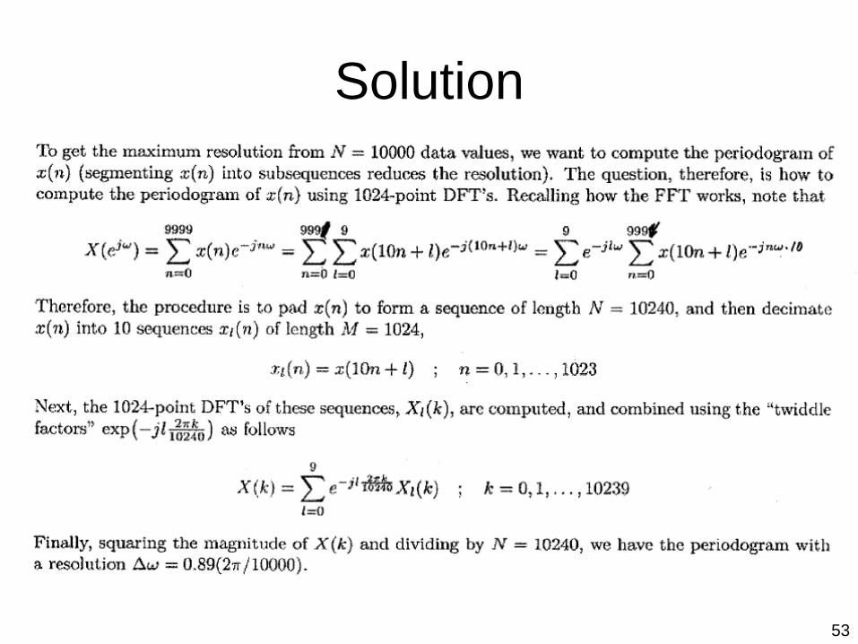
Solution

54
Solution
55
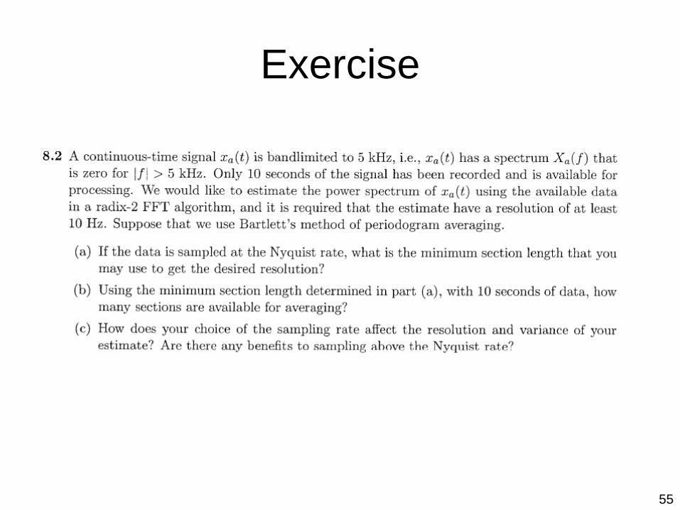
Exercise

56
Solution

57
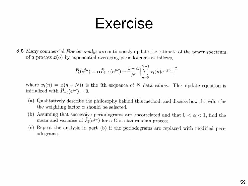
Exercise

58
Solution
59
Exercise

60
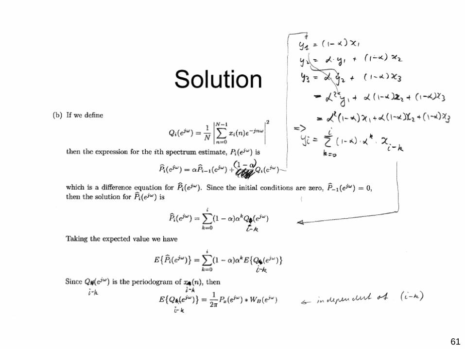
Solution
61
Solution

62
Solution

63
Solution