Speech Signal Analysis - School of Informatics

Speech Signal Analysis

Hiroshi Shimodaira and Steve Renals

Automatic Speech Recognition— ASR Lectures 2&317,21 January 2019

ASR Lectures 2&3 Speech Signal Analysis 1

Overview

Speech Signal Analysis for ASR

Features for ASR

Spectral analysis

Cepstral analysis

Standard features for ASR: FBANK, MFCCs and PLP analysis

Dynamic features

Reading:

Jurafsky & Martin, sec 9.3

P Taylor, Text-to-Speech Synthesis, chapter 12, signalprocessing background chapter 10


Speech signal analysis for ASR

AcousticModel

Lexicon

LanguageModel

Recorded Speech

SearchSpace

Decoded Text (Transcription)

TrainingData

SignalAnalysis


Speech production model

1

1

1

larynx

pharynxlips

teeth

oral cavity

Vocal Organs & Vocal Tract

nasal cavity

vocal folds

lungs

t

1

00

0

|H( )|

=1/TF

T

|V( )|

|X( )|

vocal folds

v(t)

Cavity

CavityNasal

tongue

(ï6dB/oct.)

+6dB/oct.

lipsx(t)

F2F1F3

(formants)

Lary

nx +

Mouth

Phar

ynx

ï12dB/oct.

frequency

F1F3

F2

(F0 : fundamental frequency)


A/D conversion — Sampling

Convert analogue signals in digital form

c

waveSound pressure

d

sc

c

s

s c

c

p

cc

T

t t

x (t )

tT

1

x (t ) x[t ]Conversion fromimpulse train todiscrete−time sequence

s (t )

Microphone


A/D conversion — Sampling (cont.)

Things to know:

Sampling Frequency (Fs = 1/Ts )

Speech Sufficient FsMicrophone voice (< 10kHz) 20 kHzTelephone voice (< 4kHz) 8 kHz

Analogue low-pass filtering to avoid ’aliasing’NB: the cut-off frequency should be less than theNyquist frequency (= Fs/2)


Acoustic Features for ASR

Acoustic Model

ASRFront End

Sampled signal

x(n) ot(k)

Acoustic feature vectors

Speech signal analysis to produce a sequence of acoustic featurevectors


Acoustic Features for ASR

Desirable characteristics of acoustic features used for ASR:

Features should contain sufficient information to distinguishbetween phones

good time resolution (10ms)good frequency resolution (20 ∼ 40 channels)

Be separated from F0 and its harmonics

Be robust against speaker variation

Be robust against noise or channel distortions

Have good “pattern recognition characteristics”

low feature dimensionfeatures are independent of each other (NB: this applies toGMMs, but not required for NN-based systems)


MFCC-based front end for ASR

c

dd

o [i]

e

x(t )

y [j]e

e

e

y [j],

y [j],

y [j],

x[t ] x’[t ]

x [n]

∆

∆∆∆∆

∆

2t

t

t

t

t

t

t

t

tt

t

t

t

Model

log(Y [m])

Acoustic

A/D conversion

Feature

Window

Energy

IDFTTransform

Mel filterbank

log( )

Dynamicfeatures

|X [k]|

Y [m]

DFTPreempahsis


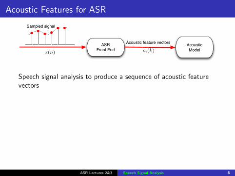
Pre-emphasis and spectral tilt

Pre-emphasis increases the magnitude of higher frequencies inthe speech signal compared with lower frequencies

Spectral Tilt

The speech signal has more energy at low frequencies (forvoiced speech)This is due to the glottal source (see the figure)

Pre-emphasis (first-order) filter boosts higher frequencies:

x ′[td ] = x [td ]− αx [td−1] 0.95 < α < 0.99


Pre-emphasis: example

Example of pre-emphasis

•  Before and after pre-emphasis

 Spectral slice from the vowel [aa]

Vowel /aa/ - time slice of the spectrum

(Jurafsky & Martin, fig. 9.9)


Windowing

The speech signal is constantly changing (non-stationary)Signal processing algorithms usually assume that the signal isstationaryPiecewise stationarity: model speech signal as a sequence offrames (each assumed to be stationary)Windowing: multiply the full waveform s[n] by a windoww [n] (in time domain):

x [n] = w [n] s[n] ( xt [n] = w [n] x ′[td +n] )

Simply cutting out a short segment (frame) from s[n] is arectangular window — causes discontinuities at the edges ofthe segmentInstead, a tapered window is usually usede.g. Hamming (α = 0.46164) or Hanning (α = 0.5) window

w [n] = (1−α)− α cos

(2πn

L−1

)L : window width


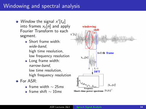
Windowing and spectral analysis

Window the signal x ′[td ]into frames xt [n] and applyFourier Transform to eachsegment.

Short frame width:wide-band,high time resolution,low frequency resolutionLong frame width:narrow-band,low time resolution,high frequency resolution

For ASR:

frame width ∼ 25msframe shift ∼ 10ms

frame

DFT

t+1 th

Short−time power spectrum

shift

windowing

Magn

itu

de

Frequency

d

|X [k]|

x’[t ]

|X [k]|

x [n]

0 L−1

t+1

2

2

t

t+1


Short-time spectral analysis

windowingshift

frame

Shortïtime power spectrum

Fourier TransformDiscrete ï

Frequency

Inte

nsity

0

10

20

30

40

50

60

70

Frequency

Time (frame)


Discrete Fourier Transform (DFT)

Purpose: extracts spectral information from a windowedsignal (i.e. how much energy at each frequency band)

Input: windowed signal x [0], . . . , x [L−1] (time domain)

Output: a complex number X [k] for each of N frequencybands representing magnitude and phase for the kth frequencycomponent (frequency domain)

Discrete Fourier Transform (DFT):

X [k] =N−1∑n=0

x [n] exp

(−j 2π

Nkn

)NB: exp(jθ) = e jθ = cos(θ) + j sin(θ)

Fast Fourier Transform (FFT) — efficient algorithm forcomputing DFT when N is a power of 2, and N ≥ L.


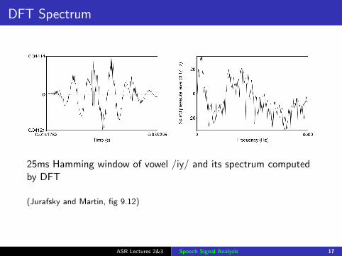
DFT Spectrum

Discrete Fourier Transform computing a spectrum

•  A 25 ms Hamming-windowed signal from [iy]

 And its spectrum as computed by DFT (plus other smoothing)

25ms Hamming window of vowel /iy/ and its spectrum computedby DFT

(Jurafsky and Martin, fig 9.12)


Wide-band and narrow-band spectrograms358 Chapter 12. Analysis of Speech Signals

Figure 12.8 Wide band spectrogram

Figure 12.9 Narrow band spectrogram

is centred around the pitch period. As pitch is generally changing, this makes the frame shiftvariable. Pitch-synchronous analysis has the advantage that each frame represents the output ofthe same process, that is, the excitation of the vocal tract with a glottal pulse. In unvoiced sections,the frame rate is calculated at even intervals. Of course, for pitch-synchronous analysis to work,we must know where the pitch periods actually are: this is not a trivial problem and will beaddressed further in section 12.7.2. Note that fixed frame shift analysis is sometimes referred toas pitch-asynchronous analysis.

Figure 12.3 shows the waveform and power spectrum for 5 different window lengths. Tosome extent, all capture the envelope of the spectrum. For window lengths of less than one period,it is impossible to resolve the fundamental frequency and so no harmonics are present. As the win-dow length increases, the harmonics can clearly be seen. At the longest window length, we havea very good frequency resolution, but because so much time-domain waveform is analysed, theposition of the vocal tract and pitch have changed over the analysis window, leaving the harmonicsand envelope to represent an average over this time rather than a single snapshot.

window width = 2.5ms

window width = 25ms

(Taylor, figs 12.8, 12.9)


Effect of windowing — time domain

0

0.2

0.4

0.6

0.8

1

0 200 400 600 800 1000 1200

rectangle

0

0.2

0.4

0.6

0.8

1

0 200 400 600 800 1000 1200

rectangle

0

0.2

0.4

0.6

0.8

1

0 200 400 600 800 1000 1200

rectangle

0

0.2

0.4

0.6

0.8

1

0 200 400 600 800 1000 1200

rectangle

0

0.2

0.4

0.6

0.8

1

0 200 400 600 800 1000 1200

rectangle

0

0.2

0.4

0.6

0.8

1

0 200 400 600 800 1000 1200 0

0.2

0.4

0.6

0.8

1

0 200 400 600 800 1000 1200

hammin

0

0.2

0.4

0.6

0.8

1

0 200 400 600 800 1000 1200

hammin

0

0.2

0.4

0.6

0.8

1

0 200 400 600 800 1000 1200

hammin

0

0.2

0.4

0.6

0.8

1

0 200 400 600 800 1000 1200

hammin

0

0.2

0.4

0.6

0.8

1

0 200 400 600 800 1000 1200 0

0.2

0.4

0.6

0.8

1

0 200 400 600 800 1000 1200 0

0.2

0.4

0.6

0.8

1

0 200 400 600 800 1000 1200

hannin

0

0.2

0.4

0.6

0.8

1

0 200 400 600 800 1000 1200

hannin

0

0.2

0.4

0.6

0.8

1

0 200 400 600 800 1000 1200

hannin

Rectangular Hamming Hanning352 Chapter 12. Analysis of Speech Signals

-1

-0.5

0

0.5

1

0 100 200 300 400 500

amplitud

e

samples

(a) Rectangular window

-1-0.8-0.6-0.4-0.2

0 0.2 0.4 0.6 0.8

1

0 100 200 300 400 500

amplitud

e

samples

(b) Hanning window

-1-0.8-0.6-0.4-0.2

0 0.2 0.4 0.6 0.8

1

0 100 200 300 400 500

amplitud

e

samples

(c) Hamming window

Figure 12.1 Effect of windowing in the time domain

shows a spike at the sinusoid frequency, but also shows prominent energy on either side. Thiseffect is much reduced in the hanning window. In the log version of this, it is clear there thereis a wider main lobe than in the rectangular case - this is the key feature as it means that moreenergy is allowed to pass through at this point in comparison with the neighbouring frequencies.The hamming window is very similar to the hanning, but has the additional advantage that the sidelobes immediately neighbouring the main lobe are more suppressed. Figure 12.3 shows the effectof the windowing operation on a square wave signal and shows that the harmonics are preservedfar more clearly in the case where the Hamming window is used.

12.1.2 Short term spectral representations

Using windowing followed by a DFT, we can generate short term spectra from speech wave-forms. The DFT spectrum is complex and and can be represented by its real and imaginary partsor its magnitude and phase parts. As explained in section 10.1.5 the ear is not sensitive to phaseinformation in speech, and so the magnitude spectrum is the most suitable frequency domain rep-resentation. The ear interprets sound amplitude in an approximately logarithmic fashion - so adoubling in sound only produces an additive increase in perceived loudness. Because of this, it isusual to represent amplitude logarithmically, most commonly on the decibel scale. By convention,we normally look at the log power spectrum, that is the log of the square of the magnitude spec-trum. These operations produce a representation of the spectrum which attempts to match humanperception: because phase is not perceived, we use the power spectrum, and because our responseto signal level is logarithmic we use the log power spectrum.

(Taylor, fig 12.1)


Effect of windowing — frequency domain

-60

-50

-40

-30

-20

-10

0

0 0.2 0.4 0.6 0.8 1

log magnitude [dB]

Normalised freqency [f/pi]

|X(w)|

-1

-0.5

0

0.5

1

0 50 100 150 200

time

x[n]

-60

-50

-40

-30

-20

-10

0

0 0.2 0.4 0.6 0.8 1

log magnitude [dB]


Rectangle

-60

-50

-40

-30

-20

-10

0

0 0.2 0.4 0.6 0.8 1

log magnitude [dB]


Hamming

-60

-50

-40

-30

-20

-10

0

0 0.2 0.4 0.6 0.8 1

log magnitude [dB]


Hanning

-60

-50

-40

-30

-20

-10

0

0 0.2 0.4 0.6 0.8 1

log magnitude [dB]


Blackman

x(t) = 0.15 sin(2πf1t) + 0.85 sin(2πf2t + 0.3)f1 = 0.13, f2 = 0.22


Effect of windowing — frequency domain

-0.1

0

0.1

0.2

0.3

0.4

0.5

0 0.2 0.4 0.6 0.8 1

Magnitute


|X(w)|

-1

-0.5

0

0.5

1

0 50 100 150 200

time

x[n]

-0.1

0

0.1

0.2

0.3

0.4

0.5

0 0.2 0.4 0.6 0.8 1

Magnitute


Rectangle

-0.1

0

0.1

0.2

0.3

0.4

0.5

0 0.2 0.4 0.6 0.8 1

Magnitute


Hamming

-0.1

0

0.1

0.2

0.3

0.4

0.5

0 0.2 0.4 0.6 0.8 1

Magnitute


Hanning

-0.1

0

0.1

0.2

0.3

0.4

0.5

0 0.2 0.4 0.6 0.8 1

Magnitute


Blackman

x(t) = 0.15 sin(2πf1t) + 0.85 sin(2πf2t + 0.3)f1 = 0.13, f2 = 0.22


DFT Spectrum Features for ASR

Equally-spaced frequency bands — but human hearing lesssensitive at higher frequencies (above ∼ 1000Hz)

The estimated power spectrum contains harmonics of F0,which makes it difficult to estimate the envelope of thespectrum

4 6 8

10 12

0 50 100 150 200 250

Log |X(w)|

Frequency bins of STFT are highly correlated each other, i.e.power spectrum representation is highly redundant


Human hearing

Physical quality Perceptual qualityIntensity Loudness

Fundamental frequency PitchSpectral shape Timbre

Onset/offset time TimingPhase difference in binaural hearing Location

Technical terms

equal-loudness contours

masking

auditory filters (critical-band filters)

critical bandwidth


Equal loudness contour


Nonlinear frequency scaling

Human hearing is less sensitive to higher frequencies — thushuman perception of frequency is nonlinear

Mel scale

M(f ) = 1127 ln(1 + f /700)

Bark scale

b(f ) = 13 arctan(0.00076f )

+ 3.5 arctan((f /7500)2)

Linear frequency [Hz]

0

1500

2000

2500

2000 4000 6000 8000 10000 12000 14000

500

1000

3000

3500

Mel fr

equency [M

el]

0

MelBark

ln()

12000 10000 8000 6000 4000 0 0

0.2

0.6

0.8

1.0

2000

Linear frequency [Hz]

0.4W

arp

ed

no

rma

lize

d f

req

ue

ncy


Mel-Filter Bank

Apply a mel-scale filter bank to DFT power spectrum toobtain mel-scale power spectrumEach filter collects energy from a number of frequency bandsin the DFTLinearly spaced < 1000 Hz, logarithmically spaced > 1000 Hz

2

Y[m]

|X[k]|

Triangular band−pass filters

Mel−scale power spectrum

DFT(STFT) power spectrum

Frequency bins1 2 N

1 2 M


Mel-Filter Bank (cont.)

Yt [m] =N∑

k=1

Wm[k] |Xt [k]|2

where k : DFT bin number (1, . . . ,N)m : mel-filter bank number (1, . . . ,M).

How many number of mel-filter channels?

≈ 20 for GMM-HMM based ASR20 ∼ 40 for DNN (+HMM) based ASR


Log Mel Power Spectrum

Compute the log magnitude squared of each mel-filter bankoutput: logY [m]

Taking the log compresses the dynamic rangeHuman sensitivity to signal energy is logarithmic — i.e.humans are less sensitive to small changes in energy at highenergy than small changes at low energyLog makes features less variable to acoustic coupling variationsRemoves phase information — not important for speechrecognition (not everyone agrees with this)

Aka “log mel-filter bank outputs” or “FBANK features”,which are widely used in recent DNN-HMM based ASRsystems


DFT Spectrum Features for ASR

Equally-spaced frequency bands — but human hearing lesssensitive at higher frequencies (above ∼ 1000Hz)

The estimated power spectrum contains harmonics of F0,which makes it difficult to estimate the envelope of thespectrum

4 6 8

10 12

0 50 100 150 200 250

Log |X(w)|

Frequency bins of STFT are highly correlated each other, i.e.power spectrum representation is highly redundant


Cepstral Analysis

Source-Filter model of speech production

Source: Vocal cord vibrations create a glottal source waveformFilter: Source waveform is passed through the vocal tract:position of tongue, jaw, etc. give it a particular shape andhence a particular filtering characteristic

Source characteristics (F0, dynamics of glottal pulse) do nothelp to discriminate between phones

The filter specifies the position of the articulators

... and hence is directly related to phone discrimination

Cepstral analysis enables us to separate source and filter


Cepstral Analysis

Split power spectrum into spectral envelope and F0 harmonics.

4 6 8

10 12

0 50 100 150 200 250

Log |X(w)|

0 0.1 0.2 0.3 0.4 0.5 0.6 0.7 0.8 0.9

0 50 100 150 200 250

Cepstrum

4 6 8

10 12

0 50 100 150 200 250

Envelope (Lag=30)

0 2 4 6 8

10

0 50 100 150 200 250

Residue

Log spectrum (freq domain)

⇓ Inverse Fourier Transform

Cepstrum (time domain) (quefrency)⇓ Liftering to get low/high part

(lifter: filter used in cepstral domain)

⇓ Fourier Transform

Smoothed log spectrum (freq domain)[low-part of cepstrum]

+

Fine structure[high-part of cepstrum]


The Cepstrum

Cepstrum obtained by applying inverse DFT to log magnitudespectrum (may be mel-scaled)

Cepstrum is time-domain (we talk about quefrency)

Inverse DFT:

x [n] =1

N

N−1∑k=0

X [k] exp

(j

2π

Nnk

)Since log power spectrum is real and symmetric the inverseDFT is equivalent to a discrete cosine transform (DCT)

yt [n] =M−1∑m=0

log(Yt [m]) cos(n(m+0.5)

π

M

), n = 0, . . . , J


MFCCs

Smoothed spectrum: transform to cepstral domain, truncate,transform back to spectral domain

Mel-frequency cepstral coefficients (MFCCs): use the cepstralcoefficients directly

Widely used as acoustic features in HMM-based ASRFirst 12 MFCCs are often used as the feature vector (removesF0 information)Less correlated than spectral features — easier to model thanspectral featuresVery compact representation — 12 features describe a 20msframe of dataFor standard HMM-based systems, MFCCs result in betterASR performance than filter bank or spectrogram featuresMFCCs are not robust against noise


PLP — Perceptual Linear Prediction

y [n] =P∑

k=1

ak yt [n−k]

PLP (Hermansky, JASA 1990)

Uses equal loudness pre-emphasisand cube-root compression(motivated by perceptual results)rather than log compression

Uses linear predictiveauto-regressive modelling to obtaincepstral coefficients

PLP has been shown to lead to

slightly better ASR accuracyslightly better noiserobustness

compared with MFCCs


Dynamic features

Speech is not constant frame-to-frame, so we can add featuresto do with how the cepstral coefficients change over time

∆∗, ∆2∗ are delta features (dynamic features / timederivatives)

Simple calculation of delta features d(t) at time t for cepstralfeature c(t) (e.g. yt [j ]):

d(t) =c(t + 1)− c(t − 1)

2

More sophisticated approach estimates the temporal derivativeby using regression to estimate the slope (typically using 4frames each side)“Standard” ASR features (for GMM-based systems) are 39dimensions:

12 MFCCs, and energy12 ∆MFCCs, ∆energy12 ∆2MFCCs, ∆2energy


Estimating dynamic features

timet0

0

c(t)

’c (t )


Feature Transforms

Orthogonal transformation (orthogonal bases)

DCT (discrete cosine transform)PCA (principal component analysis)

Transformation based on the bases that maximises theseparability between classes.

LDA (linear discriminant analysis) / Fisher’s lineardiscriminantHLDA (heteroscedastic linear discriminant analysis)


Feature Normalisation

Basic Idea: Transform the features to reduce mismatchbetween training and test

Cepstral Mean Normalisation (CMN): subtract the averagefeature value from each feature, so each feature has a meanvalue of 0. makes features robust to some linear filtering ofthe signal (channel variation)

Cepstral Variance Normalisation (CVN): Divide feature vectorby standard deviation of feature vectors, so each featurevector element has a variance of 1

Cepstral mean and variance normalisation, CMN/CVN:

yt [j ] =yt [j ]− µ(y [j ])

σ(y [j ])

Compute mean and variance statistics over longest availablesegments with the same speaker/channel

Real time normalisation: compute a moving average


Acoustic features in state-of-the-art ASR systems

See Tables 1, 2, and 3 in

Jinyu Li, Dong Yu, Jui-Ting Huang, and Yifan Gong,“Improving Wideband Speech Recognition Using Mixed-BandwidthTraining Data In CD-DNN-HMM”,2012 IEEE Workshop in Spoken Language Technology (SLT2012).https://doi.org/10.1109/SLT.2012.6424210


https://doi.org/10.1109/SLT.2012.6424210

Summary: Speech Signal Analysis for ASR

Good characteristics of ASR features

FBANK features

Short-time DFT analysisMel-filter bankLog magnitude squaredWidely used for DNN ASR (M ≈ 40)

MFCCs - mel frequency cepstral coefficients

FBANK featuresInverse DFT (DCT)Use first few (12) coefficientsWidely used for GMM-HMM ASR

Delta features (dynamic features)

39-dimension feature vector (for GMM-HMM ASR):MFCC-12 + energy; + Deltas; + Delta-Deltas


References

J&M: Daniel Jurafsky and James H. Martin (2008). Speechand Language Processing, Pearson Education (2nd edition).

Taylor: Paul Taylor (2009). Text-to-Speech Synthesis,Cambridge University Press.

Hynek Hermansky, “Perceptual linear predictive (PLP)analysis of speech,” The Journal of the Acoustical Society ofAmerica, Vol.87, No.4, pp.1737–1752, 1980.


Documents

Speech Signal Analysis - School of Informatics