Speed Control With Low ArmaSpeed Control With Low Armature Loss for Very Small Sensoture Loss for Very Small Senso

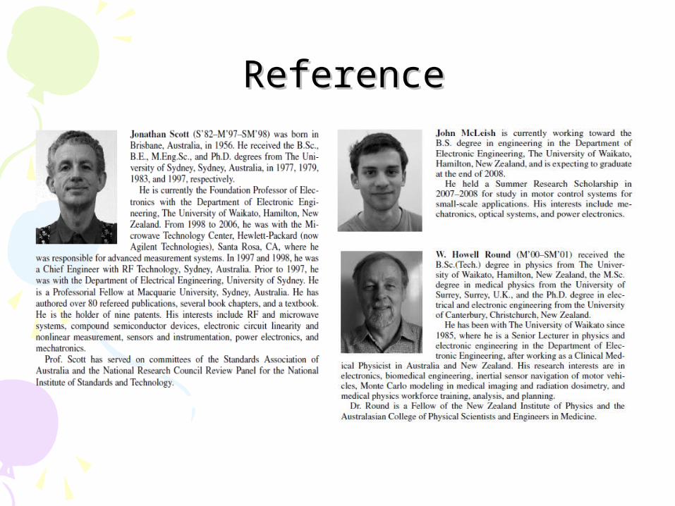
rless Brushed DC Motorsrless Brushed DC MotorsJonathan Scott, Jonathan Scott, Senior Member, IEEESenior Member, IEEE, John McLeish, and W. Howell Round, , John McLeish, and W. Howell Round, Senior MeSenior Me

mber, IEEEmber, IEEE

Adviser : Ming-Shyan Wang

Student : Ping-Hung Huang

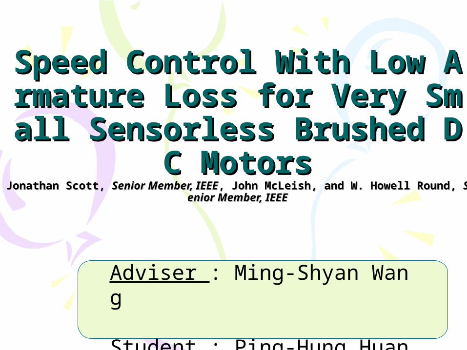
AbstractA method for speed control of brushed dc motors is presented. It is particularly applicable to motors with armatures of less than 1 cm3. Motors with very small armatures are difficult to control using the usual pulsewidth-modulation (PWM) approach and are apt to overheat if so driven. The technique regulates speed via the back electromotive force but does not require currentdiscontinuousdrives.

Armature heating in small motors under PWM drive is explained and quantified. The method is verified through simulation and measurement. Control is improved, and armature losses are minimized. The method can expect to findapplication in miniature mechatronic equipment.

Index Terms—DC motor drives, micromotors, (PM) motors, pulsewidth modulation (PWM), rotating machine stability, variable-speed drives.

I. INTRODUCTIONLow-cost and mechanically small brushed motors do not have a dedicated shaft sensor; therefore,back-electromotive-force (EMF) sensing is the established way to sense speed.

With pulsewidth modulation (PWM), speed sensing is achieved by running the motor in discontinuous-conduction mode and directly sampling the back EMF that appears on the terminals after inductive flyback currents subside.

It is possible to estimate speed by more complicated means, but this is not common.

Problems arise when this method is applied to very small motors.The plant contains two real poles, and the speed sensor adds a zeroth-order hold.

One pole is chiefly defined by the rotating mass of the system; this pole is typically the dominant one and can vary with mechanical load.

The hold arises because the speed is sensed only once per period of the PWM drive, when the back EMF is exposed during the off part of the drive cycle, after the inductive freewheel period.

This rate, the PWM frequency, is typically 50–400 Hz. In the case of very small motors, the mechanical pole and PWM frequency lie close together.

Because the drive must be current discontinuous, the motor inductance limits the maximum PWM frequency and, therefore, also the rate at which the speed is sampled.

Problems arise when this method is applied to very small motors.The plant contains two real poles, and the speed sensor adds a zeroth-order hold.

Motor 1 is a low-cost cellphone vibrator motor of a closed-can design with an armature of approximately0.04 cm3.

Motor 2 is a high-quality motor with an armature of Approximately 0.3 cm3 designed to use shaft-drivenconvective cooling, unlike motor 1 that is in a sealed can.

As appropriate,one or the other motor, or a comparison between the two will be used in this paper.

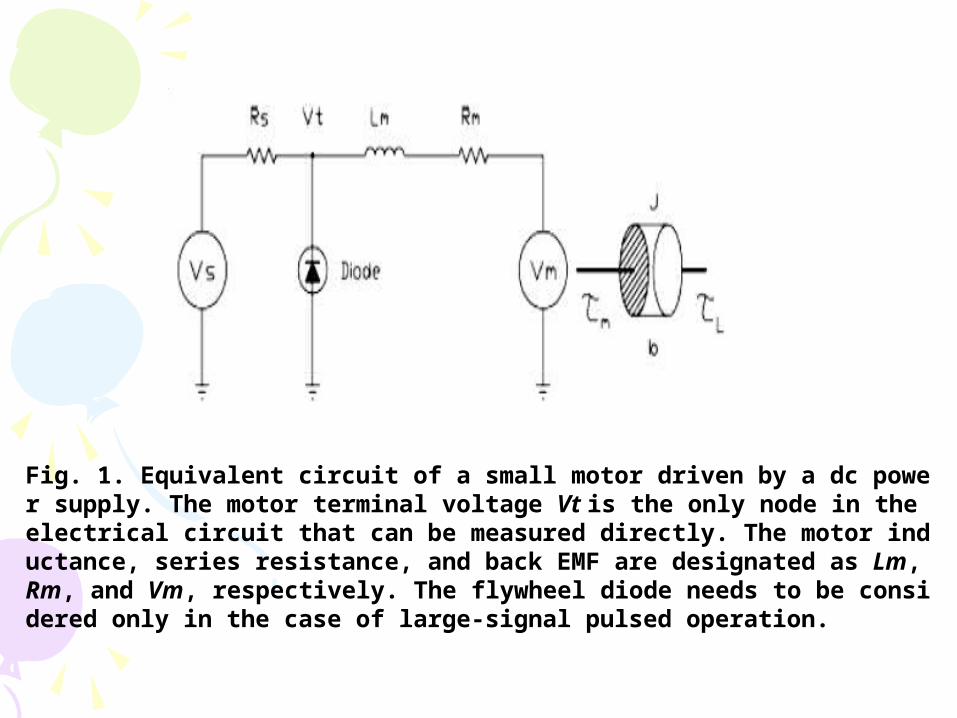
Fig. 1. Equivalent circuit of a small motor driven by a dc power supply. The motor terminal voltage Vt is the only node in the electrical circuit that can be measured directly. The motor inductance, series resistance, and back EMF are designated as Lm, Rm, and Vm, respectively. The flywheel diode needs to be considered only in the case of large-signal pulsed operation.

II. Negative-Ressistance Control

A. Practical Implementation

B. Controller Stability

C. Adaptive Tuning

II. NEGATIVE-RESISTANCE CONTROL

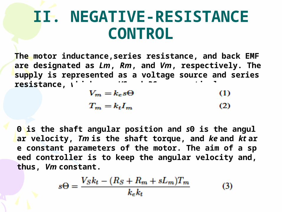
The motor inductance,series resistance, and back EMF are designated as Lm, Rm, and Vm, respectively. The supply is represented as a voltage source and series resistance, which are VS and RS, respectively.

Θ is the shaft angular position and sΘ is the angular velocity, Tm is the shaft torque, and ke and kt are constant parameters of the motor. The aim of a speed controller is to keep the angular velocity and, thus, Vm constant.

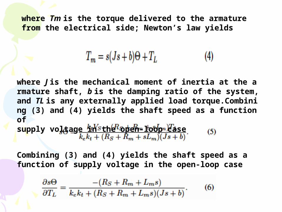
Combining (3) and (4) yields the shaft speed as a function of supply voltage in the open-loop case

where Tm is the torque delivered to the armature from the electrical side; Newton’s law yields

where J is the mechanical moment of inertia at the armature shaft, b is the damping ratio of the system, and TL is any externally applied load torque.Combining (3) and (4) yields the shaft speed as a function ofsupply voltage in the open-loop case

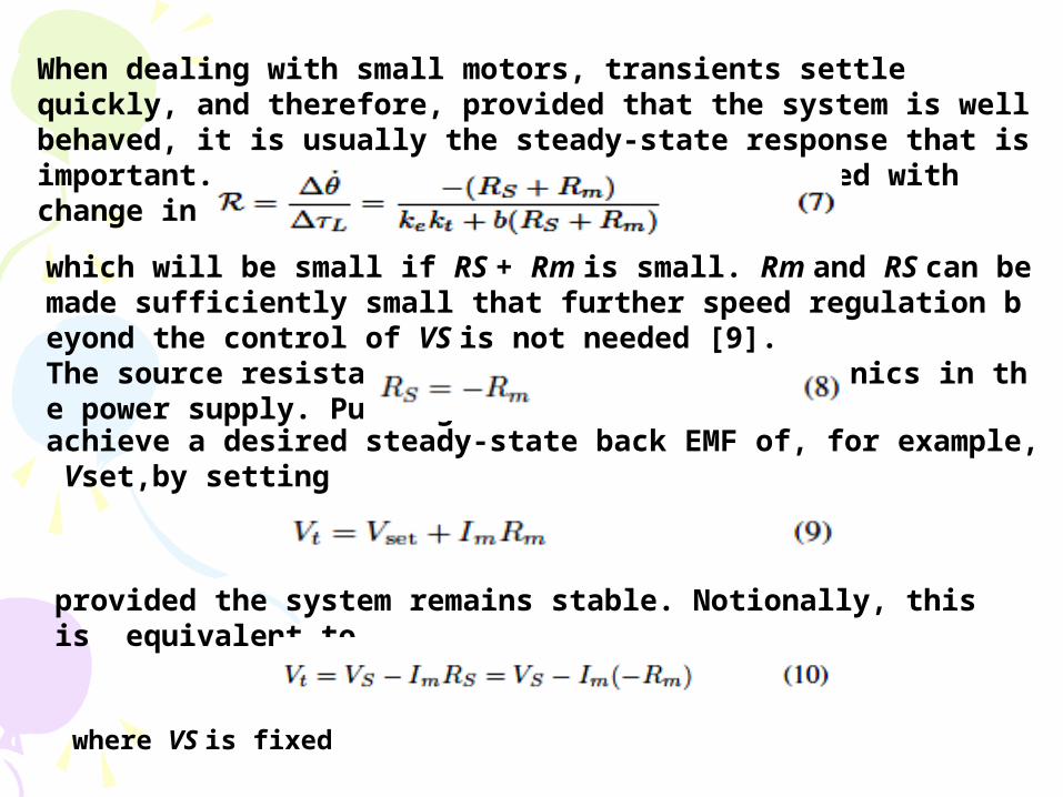
When dealing with small motors, transients settle quickly, and therefore, provided that the system is well behaved, it is usually the steady-state response that is important. Let the steady-state change in speed with change in load be

which will be small if RS + Rm is small. Rm and RS can be made sufficiently small that further speed regulation beyond the control of VS is not needed [9]. The source resistance RS can be set by electronics in the power supply. Putting

achieve a desired steady-state back EMF of, for example, Vset,by setting

provided the system remains stable. Notionally, this is equivalent to

where VS is fixed

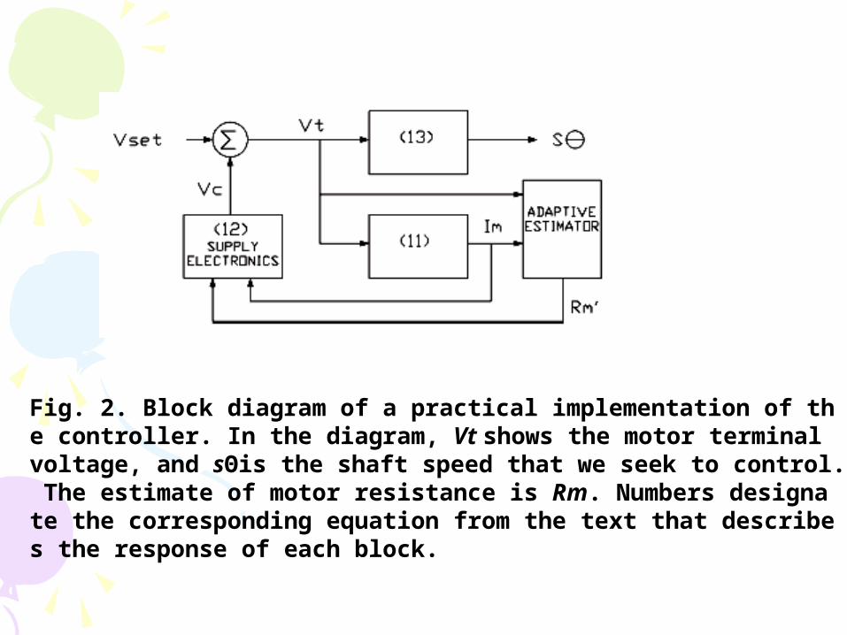
Fig. 2. Block diagram of a practical implementation of the controller. In the diagram, Vt shows the motor terminal voltage, and sΘis the shaft speed that we seek to control. The estimate of motor resistance is Rm. Numbers designate the corresponding equation from the text that describes the response of each block.

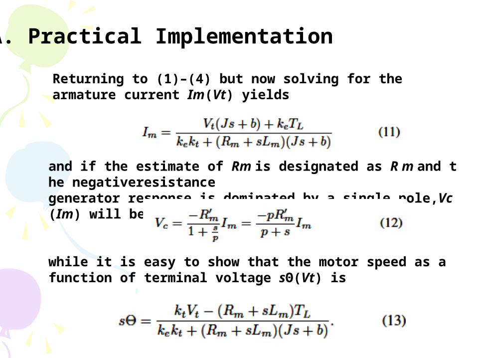
A. Practical Implementation

Returning to (1)–(4) but now solving for the armature current Im(Vt) yields

and if the estimate of Rm is designated as R m and the negativeresistancegenerator response is dominated by a single pole,Vc(Im) will be

while it is easy to show that the motor speed as a function of terminal voltage sΘ(Vt) is

B. Controller Stability

The control loop of Fig. 2 has the characteristic equation

The control loop of Fig. 2 has the characteristic equation

a cubic in canonical form As3 + Bs2 + Cs + D = 0.

Trivially, A > 0 and B > 0, while C > 0 if

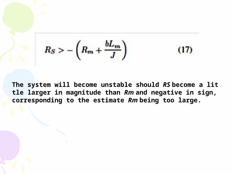
The system will become unstable should RS become a little larger in magnitude than Rm and negative in sign, corresponding to the estimate Rm being too large.

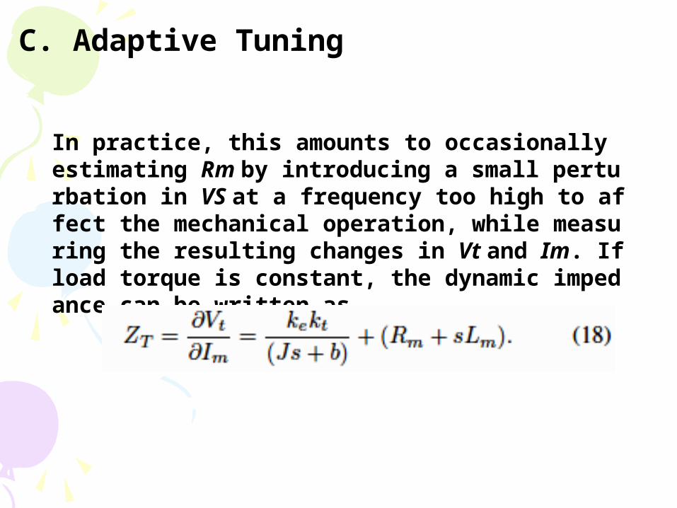
C. Adaptive Tuning

In practice, this amounts to occasionally estimating Rm by introducing a small perturbation in VS at a frequency too high to affect the mechanical operation, while measuring the resulting changes in Vt and Im. If load torque is constant, the dynamic impedance can be written as

III. SIMULATION

It was asserted in Section I that feedback control was problematic in the case of very small motors. In this section, this assertion will be demonstrated quantitatively by means of simulation.

Fig. 3 shows a number of speed-time traces simulated

for motor 1, shown in Fig. 4.

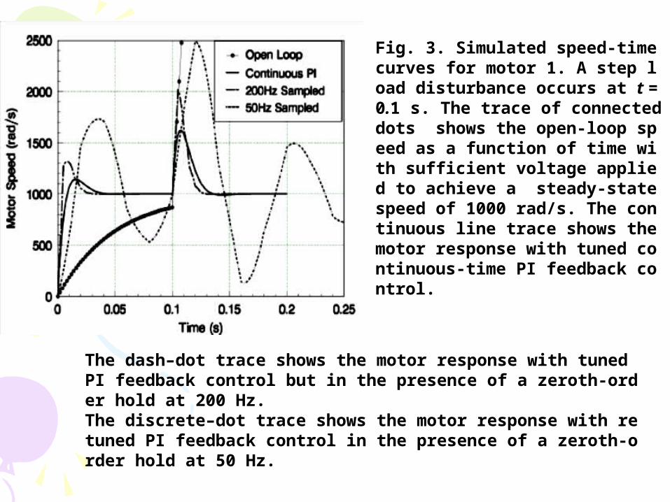
Fig. 3. Simulated speed-time curves for motor 1. A step load disturbance occurs at t = 0.1 s. The trace of connected dots shows the open-loop speed as a function of time with sufficient voltage applied to achieve a steady-state speed of 1000 rad/s. The continuous line trace shows the motor response with tuned continuous-time PI feedback control.

The dash–dot trace shows the motor response with tuned PI feedback control but in the presence of a zeroth-order hold at 200 Hz. The discrete–dot trace shows the motor response with retuned PI feedback control in the presence of a zeroth-order hold at 50 Hz.

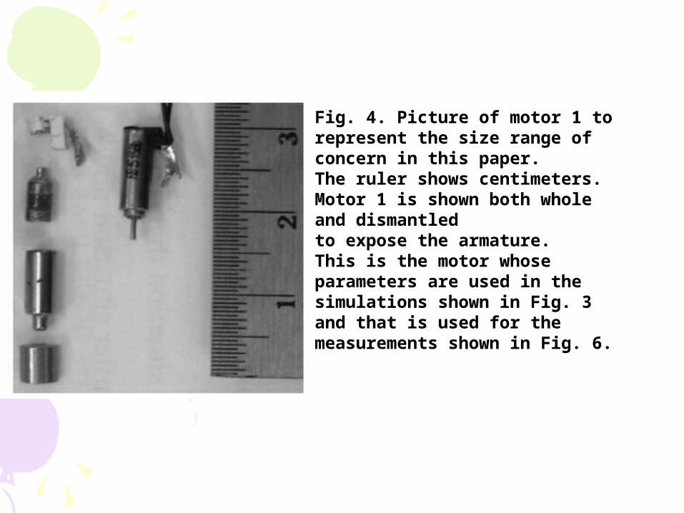
Fig. 4. Picture of motor 1 to represent the size range of concern in this paper.The ruler shows centimeters. Motor 1 is shown both whole and dismantledto expose the armature. This is the motor whose parameters are used in the simulations shown in Fig. 3 and that is used for the measurements shown in Fig. 6.

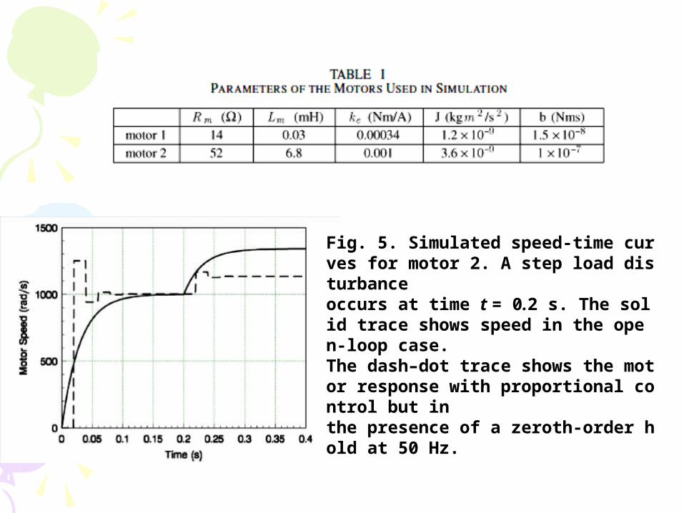
Fig. 5. Simulated speed-time curves for motor 2. A step load disturbanceoccurs at time t = 0.2 s. The solid trace shows speed in the open-loop case.The dash–dot trace shows the motor response with proportional control but inthe presence of a zeroth-order hold at 50 Hz.

IV. MEASURED RESULTS

B. Speed Regulation

A. Motor Heating

A. Motor Heating

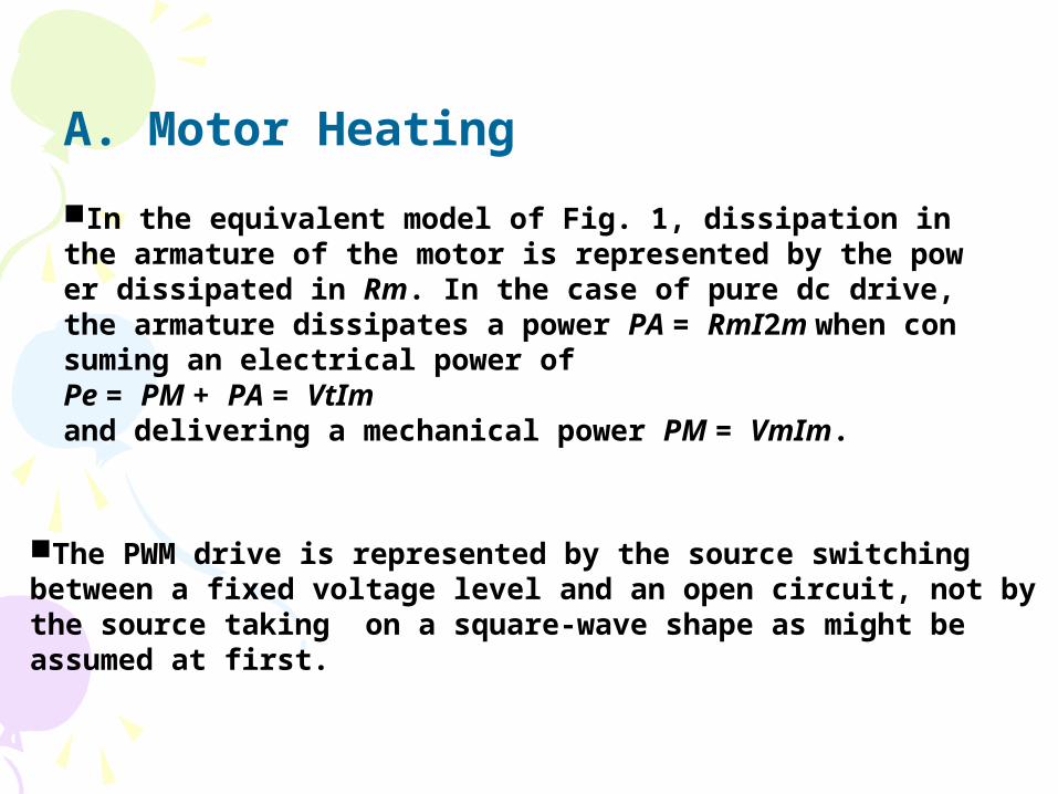
In the equivalent model of Fig. 1, dissipation in the armature of the motor is represented by the power dissipated in Rm. In the case of pure dc drive, the armature dissipates a power PA = RmI2m when consuming an electrical power of Pe = PM + PA = VtIm and delivering a mechanical power PM = VmIm.

The PWM drive is represented by the source switching between a fixed voltage level and an open circuit, not bythe source taking on a square-wave shape as might be assumed at first.

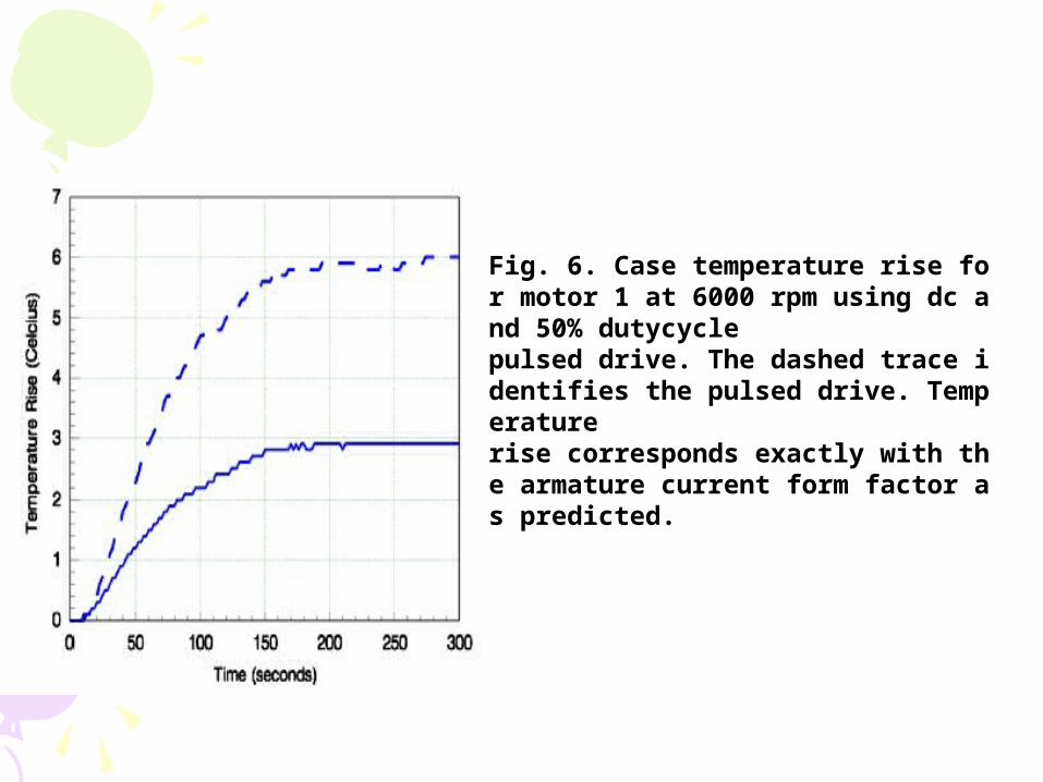
Fig. 6. Case temperature rise for motor 1 at 6000 rpm using dc and 50% dutycyclepulsed drive. The dashed trace identifies the pulsed drive. Temperaturerise corresponds exactly with the armature current form factor as predicted.

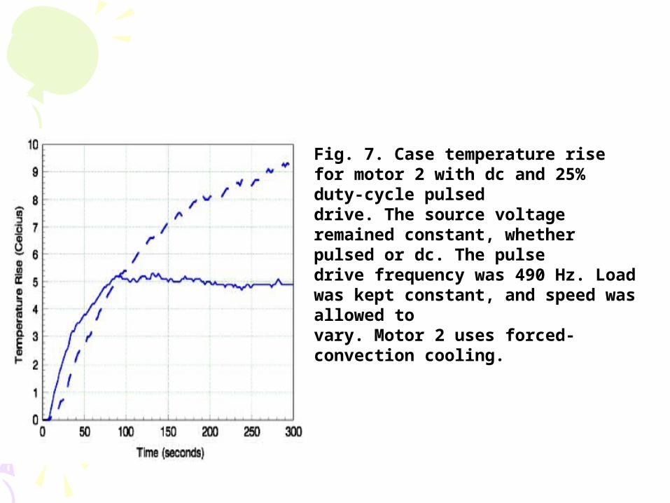
Fig. 7. Case temperature rise for motor 2 with dc and 25% duty-cycle pulseddrive. The source voltage remained constant, whether pulsed or dc. The pulsedrive frequency was 490 Hz. Load was kept constant, and speed was allowed tovary. Motor 2 uses forced-convection cooling.

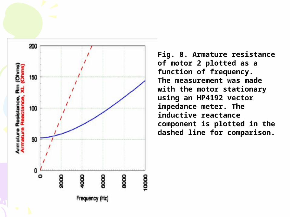
Fig. 8. Armature resistance of motor 2 plotted as a function of frequency.The measurement was made with the motor stationary using an HP4192 vectorimpedance meter. The inductive reactance component is plotted in the dashed line for comparison.

B. Speed Regulation

In order to demonstrate the viability of this approach, both a fixed negative-R controller and an elementary adaptive version were implemented.

These were compared with four alterna-tives, namely, plain constant-voltagedrive,two commercially available EMF-sensing proportional-only PWM feedback controllers,and an EMF-sensing controller that can implementproportional–integral–derivative (PID) control.

It is customary to test a motor with a mechanical arrangement that can apply a known constant load torque, such as a disk brake with the caliper applying force to a scale.

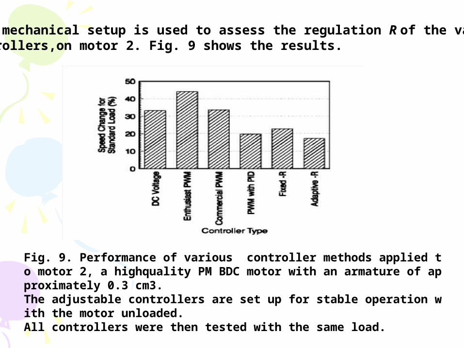
Fig. 9. Performance of various controller methods applied to motor 2, a highquality PM BDC motor with an armature of approximately 0.3 cm3. The adjustable controllers are set up for stable operation with the motor unloaded.All controllers were then tested with the same load.

This mechanical setup is used to assess the regulation R of the various controllers,on motor 2. Fig. 9 shows the results.

The PID controller had a 125-Hz PWM frequency, while the design in [12] used 200 Hz and and the design in [13] used 50 Hz. The PID controller is tuned to give modest overshoot and, therefore, has a long settling time.

The 15-s measurement duration explains why it yields a speed error.

It is clear that, in the case of this small motor, even the commercial controller is worse than a well-regulated dc supply. To an extent, this is not surprising for two reasons:

The controller described in [13] was on the edge of stability with an unloaded motor; therefore, it was possible to conclude that it had a good choice of loop gain given the constraint of unconditional stability

2. The controller described in [13] was on the edge of stability with an unloaded motor; therefore, it was possible to conclude that it had a good choice of loop gain given the constraint of unconditional stability

1. The purchased controllers did not allow loop gain to be changed but were factory preset, and they necessarily present a high impedance for a part of the cycle to expose the back EMF as noted earlier

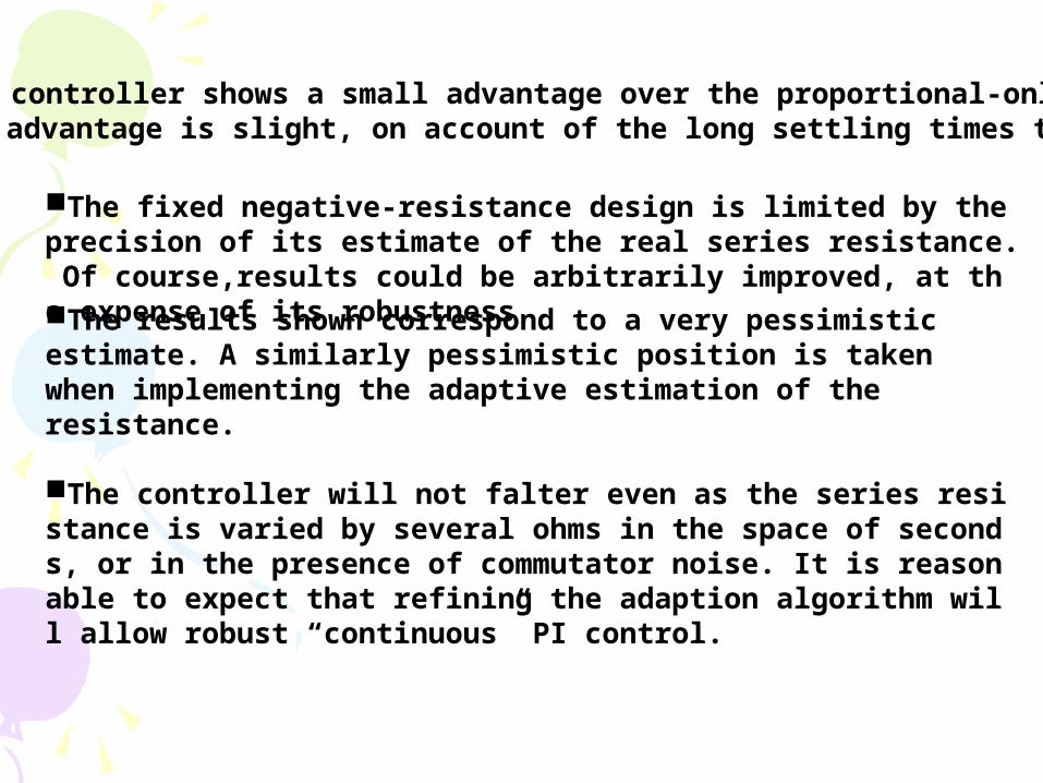
The PID controller shows a small advantage over the proportional-only designs, but this advantage is slight, on account of the long settling times that result

The fixed negative-resistance design is limited by the precision of its estimate of the real series resistance. Of course,results could be arbitrarily improved, at the expense of its robustness

The results shown correspond to a very pessimistic estimate. A similarly pessimistic position is taken when implementing the adaptive estimation of the resistance.

The controller will not falter even as the series resistance is varied by several ohms in the space of seconds, or in the presence of commutator noise. It is reasonable to expect that refining the adaption algorithm will allow robust “continuous” PI control.

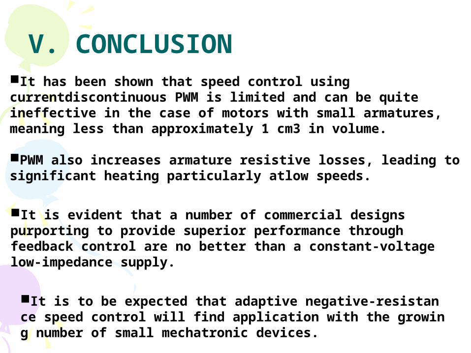
V. CONCLUSION

It is to be expected that adaptive negative-resistance speed control will find application with the growing number of small mechatronic devices.

It has been shown that speed control usingcurrentdiscontinuous PWM is limited and can be quite ineffective in the case of motors with small armatures,meaning less than approximately 1 cm3 in volume.

PWM also increases armature resistive losses, leading tosignificant heating particularly atlow speeds.

It is evident that a number of commercial designs purporting to provide superior performance through feedback control are no better than a constant-voltagelow-impedance supply.

ReferenceReference

ReferenceReference