Embed Size (px)
Citation preview

8/11/2019 Speed Delay
http://slidepdf.com/reader/full/speed-delay 1/141
AN
ANALYSIS
OF
TRAVEL
SPEED AND
DELAY
ON
A
HIGH' VOL
UME
HIGHWA Y

8/11/2019 Speed Delay
http://slidepdf.com/reader/full/speed-delay 2/141

8/11/2019 Speed Delay
http://slidepdf.com/reader/full/speed-delay 3/141
AN
ANALYSIS
OP
TRAVEL
SPEED
AND
DEIAY
ON A
HIGH-
VOLUME
HIGHWAY
To:
K.
B.
Woods,
Director
Joint
Highway
Research
Project
July
9,
1965
From:
H. L.
Michael,
Associate
Director
Project:
C-36-66C
Joint
Highway
Research
Project
Pile:
8-7-3
The
attached
report,
entitled
An
Analysis
of
Travel
Speed
and
Delay
on
a
High-Volume
Highway/'
is
part
of
the
Initial
Inventory
and
Study
for
the
project,
Evaluation
of
the
Effectiveness
of
Traffic
Engineering
Applied
to
the
US
52 Bypass.
This HPR-HPS
research
project,
C-36-66C,
was
approved
by the
Advisory
Board
on
March
6,
196k.
The
report
was
prepared
by Mr.
Theodore
B.
Treadway,
Graduate
Assistant,
under
the
direction
of
Professor
J. C.
Oppenlander.
Relationships were
developed
to
express
overall
travel
speeds
and
delays
as
functions
of
elements
that
were
descriptive
of
the
traffic
stream,
roadway
geometry,
and
roadside
development.
These
equations
permit
the
quantitative
evaluation
of
traffic
engineering
improvements
designed
to
reduce
the
travel
time
on
the
study
bypass.
The
report
is
presented
for the
record
and
will be
submitted
to
the
Highway
Commission
and
the
Bureau
of Public
Roads
for
review
and
comment.
Respectfully
submitted,
Harold L.
Michael,
Secretary
HLM:bc
Attachment
Copies:
P.
L.
Ashbaucher
p. B.
Mendenhall
J.
R.
Cooper
R.
D.
Miles
J. W.
Delleur
J.
C.
Oppenlander
W.
L.
Dolch
W.
P.
Privette
W.
H.
Goetz
M.
B.
Scott
P.
F.
Havey
j.
v.
Smythe
P.
S.
Hill
F.
w.
Stubbs
G.
A.
Leonards
E.
J.
Yoder
J. P.
McLaughlin
J. W.
Delleur

8/11/2019 Speed Delay
http://slidepdf.com/reader/full/speed-delay 4/141
final
Report
AN
ANALYSIS
OF
TRAVEL
SPEED
AND
DEIAY
ON
A
HIGH-VOLUME
HIGHWAY
by
Theodore B.
Treadvay
Graduate
Assistant
Joint
Highvay
Research
Project
Project:
C-36-66C
Pile;
8-7-3
as
Part of an
Investigation
Conducted
by
Joint Highway
Research Project
Engineering
Experiment
Station
Purdue
University
in
cooperation
with
Indiana
State
Highway
Commission
and
the
Bureau
of
Public
Roads
U
S
Department
of
Commerce
School
of Civil
Engineering
Purdue
University
Lafayette,
Indiana
July
9,
1965
Not
Reviewed
By
Indiana
State
Eighway
Commission
or
the
Bureau
of
Public
Roads
Not
Released
For
Publication
Subject
to
Change
8/11/2019 Speed Delay
http://slidepdf.com/reader/full/speed-delay 5/141
Digitized
by
the
Internet
Archive
in
2011 with
funding from
LYRASIS members and Sloan Foundation;
Indiana
Department of Transportation
http://www.archive.org/details/analysisoftravel6510trea

8/11/2019 Speed Delay
http://slidepdf.com/reader/full/speed-delay 6/141
ii
ACKNOWLEDGMENT
S
The
author
is indebted
to Professor
J.
C.
Oppenlander
for his guidance
throughout the study and his
critical
review
of
the manuscript.
Thanks
are
also
extended to
Professors
Harlley
E.
McKean
and
William
L.
Grecco for
their reviews
of
the
manuscript.
Professor
A.
D.
M.
Lewis
is acknowledged for his aid
in
the
computer
programming
and
Mr.
Robert
A.
McLean
for
his
advice
in
the
statistical
analysis.
The
assistance of
Mr.
Gordon
A.
Shunk
and
Mr.
Arvid
0.
Peterson
in
the data
collection
is
also appreciated.
8/11/2019 Speed Delay
http://slidepdf.com/reader/full/speed-delay 7/141
iii
TABLE
OF CONTENTS
Page
LIST
OF TABLES
v
LIST
OF
FIGURES
vii
ABSTRACT
ix
INTRODUCTION
1
REVIEW
OF
LITERATURE
4
Travel Times, Travel
Speeds,
and
Delays
....
4
Fundamental Concepts
5
Methods
of
Field
Measurement
6
Travel Times
6
Delays
at
Signalized Intersections
....
10
Variables
Influencing
Travel Speeds and
Delays
.
12
Multivariate Analysis
Techniques
15
Factor Analysis 16
Multiple
Linear
Regression
and
Correlation
Analysis
17
PROCEDURE
19
Design
of
Study 19
Collection of
Data
27
Analysis of
Data 30
Preliminary
Data
Processing
30
Multivariate Analyses
34
Factor Analysis
.....
34
Multiple
Linear
Regression and
Correlation
Analysis
37
Mathematical
Models
40
RESULTS
41
Uninterrupted
Flow
41
Factor
Analysis
..........
.
43
Multiple
Linear Regression
and Correlation
Analysis
57
8/11/2019 Speed Delay
http://slidepdf.com/reader/full/speed-delay 8/141
iv
TABLE OF
CONTENTS
(continued)
Page
Interrupted
Flow
.
60
Factor
Analysis
65
Multiple
Linear
Regression
and
Correlation
Analysis
76
Recommended
Improvements 81
Short-Range Improvements
.
.
83
Long-Range Improvements
........
85
SUMMARY
OF RESULTS
AND
CONCLUSIONS
86
SUGGESTIONS
FOR FURTHER RESEARCH
89
BIBLIOGRAPHY
91
References 92
Computer
Programs
.......... .
95
APPENDICES
96
Appendix
A
-
Test Sections,
U.S.
52
Bypass
...
97
Appendix
B -
Summary
Data
119
8/11/2019 Speed Delay
http://slidepdf.com/reader/full/speed-delay 9/141
LIST
OF
TABLES
Table
Page
1.
Average Overall Travel Speeds,
Uninterrupted
Flow
42
2.
Rotated-Factor
Matrix, Uninterrupted
Flow
.
44
3.
Factor-Score
Matrix, Uninterrupted
Flow
...
51
4.
Correlation
of
Mean Travel
Speed
with
Factors, Uninterrupted
Flow
54
5.
Multiple Linear
Regression and
Correlation
Analysis,
Uninterrupted
Flow
59
6.
Average Travel
Speeds,
Interrupted
Flow
... 61
7.
Average
Stopped
Times,
Interrupted
Flow
...
63
8.
Average Delays, Interrupted
Flow
64
9.
Rotated-Factor Matrix,
Interrupted
Flow
...
66
10.
Factor-Score
Matrix,
Interrupted
Flow
....
71
11.
Correlation
of
Mean
Travel
Speed
and
Delay
with
Factors, Interrupted
Flow
74
12.
Multiple Linear
Regression and
Correlation
Analysis, Interrupted
Flow
77
13.
Means and
Standard Deviations of
the
Study
Variables,
Uninterrupted Flow
120
14.
Correlation
of Travel Speed
with
the
Other
Variables,
Uninterrupted Flow
121
15.
Contributions of
the
13
Principal
Factors,
Uninterrupted
Flow
122
16.
Means
and
Standard
Deviations
of
the
Study
Variables,
Interrupted
Flow
123

8/11/2019 Speed Delay
http://slidepdf.com/reader/full/speed-delay 10/141
vi
LIST
OF
TABLES
(continued)
Table
^age
17.
Correlation of
Travel
Speed
and
Delay
with
the
Other
Variables,
Interrupted
Flow
. .
.
124
18.
Contributions of
the 11
Principal
Factors,
Interrupted Flow
125

8/11/2019 Speed Delay
http://slidepdf.com/reader/full/speed-delay 11/141
LIST
OF
FIGURES
vii
Figure
1.
Test
Sections of
U.S.
52
Bypass
.
2.
Flow Diagram
for
Data Processing
3.
Flow
Diagram for
Factor Analysis
4.
Flow
Diagram
for
Multiple
Linear
Regression
Analysis
5.
Average Travel Speeds
for
Sections
.
6.
Annual Average Daily Traffic
for
Sections
7.
Bypass,
Section
1
8.
Bypass
9.
Bypass
10.
Bypass
11.
Bypass
12.
Bypass
13*
Bypass
14.
Bypass
15.
Bypass
16.
Bypass
17.
Bypass
18.
Bypass
19.
Bypass
20.
Bypass
Section
2
Section
3
Section
4
Section
5
Section
6A
Section
6B
Section
7A
Section
7B
Section
8
Section
9
Section 10
Section
11
Section
12
Page
20
31
35
38
82
84
98
99
100
101
102
103
104
105
106
107
108
109
110
111
8/11/2019 Speed Delay
http://slidepdf.com/reader/full/speed-delay 12/141
viii
LIST
OF
FIGURES
(continued)
Figure
Page
21.
Bypass,
Section 13
H2
22.
Bypass,
Section
14
113
23.
Bypass,
Section
15
114
24.
Bypass, Section
16A
115
25.
Bypass,
Section
16B
116
26.
Bypass, Section
17.
117
27.
Bypass,
Section 18
118

8/11/2019 Speed Delay
http://slidepdf.com/reader/full/speed-delay 13/141
ix
ABSTRACT
Treadway,
Theodore
Barr.
MSCE,
Purdue
University,
June
1965.
An
Analysis
of
Travel
Speed
and
Delay
on *
High
-Volume
Highway
.
Major
Professor:
J.
C.
Op
j,enlander.
This investigation
was
a
part of
a
project designed
to
evaluate
the effectiveness
of
traffic engineering
applied
to problems of traffic movement
on
the
U.S.
52
Bypass
in
Lafayette,
Indiana.
The
specific
purposes of
this
research
were
to
identify
the locations
of
delays
on
the
bypass, to determine
the significant factors
causing
these
delays,
and
to
make recommendations
for
improving
the
flow
of
traffic.
The
movements of
traffic
on the
highway
were classified
as
uninterrupted
flow
between
intersections and
as
interrupted
flow
at
the
signalized intersections.
Factor
analysis
and
multiple
linear
regression
techniques were
applied to
express overall
travel
speeds
and
delays
as
functions
of
factors and variables that were
descriptive of the traffic
stream,
roadway geometry, and roadside
development.
The
most significant factors in
accounting
for the
variations in travel
speeds
of
uninterrupted
flow were the
types of roadside development (commercial,
urban,
and
8/11/2019 Speed Delay
http://slidepdf.com/reader/full/speed-delay 14/141
X
rural)
and stream
friction. Vehicular
delays
at traffic
signals were largely
dependent
on
the signal
design,
volume,
and the
chance of
whether or not
stops occurred. These
results formed
the
basis
of
suggestions for reducing
delays
on the bypass. Proposed
short-range
improvements included
the limitation
and channelization of access
points,
the
improvement of the
geometric
design of signalized
inter-
sections, and
the critical evaluation of the
signal-cycle
phases.
A
long-range
recommendation was the
reconstruc-
tion
of
the
bypass
as
a
four-lane,
divided
highway
to
provide
the proper
highway
and intersection
capacities.
8/11/2019 Speed Delay
http://slidepdf.com/reader/full/speed-delay 15/141
INTRODUCTION
The
movement of people
and goods is largely
dependent
on the
motor
vehicle.
To
insure the
safe
and efficient
operation
of
motor vehicles
at
levels
of
comfort
and
convenience
acceptable
to
the
driver, an adquate
system
of
highways
is
essential.
In
recent
years, vehicular
travel
has
increased
at a
tremendous rate.
The
construction
of new
highways
and
the
improvement
of
existing
facilities have
failed
to keep
pace
with the growth of motor-vehicle travel.
The
problem
is
especially acute
in
urban
areas,
where
major arterial
highways lack needed
capacity
for handling
the
large
movements of
intracity travel.
Many
urban
roads were
constructed
decades
ago,
when the
present
status
of
vehicular
travel was inconceivable.
Inadequate planning
and improvement of these facilities
have resulted in
con-
gestion and delays
which
are
costly
and
irritable
to
the
road
users.
Limited-access
freeways
are
being
constructed
in
large
urban
areas
to
accommodate
the
major
flows of through
and
intracity
travel. Existing arterial
highways
continue
to
play an important
role
in the movement
of traffic,
however,

8/11/2019 Speed Delay
http://slidepdf.com/reader/full/speed-delay 16/141
and they serve
as
collectors
and distributors
for
the new
expressways.
Through
sound
traffic
engineering
techniques,
the
improvement
of
these
arterial
facilities is necessary
for
the
efficient
and safe
functioning
of the
complete
trans-
portation system of
an
urban area.
With
a
large expenditure
of funds for the construction of new roads,
the continuing
renovation
of
the
present
highways
has been
largely
neglected.
A
project was undertaken
by
the
Joint
Highway
Research
Project
of
Purdue
University,
the
Indiana
State
Highway
Commission,
and
the
U.
S.
Bureau of Public Roads
to
evaluate
the effectiveness of traffic
engineering
as
applied
to
the
improvement
of
a congested
urban arterial highway.
The
purpose
of
this research investigation,
as
a
portion of
that
project,
was
a
detailed analysis
of travel
speeds and
delays on
the
highway. The
specific
objectives
of
this study
were
the
following:
l
a
Identify
the
locations
of reduced
travel
speeds
and
delays?
2.
Determine
the significant
factors and
variables
which
influence
travel
speeds
and
delays?
3.
Develop
statistical models using
these
significant
variables
to
predict travel
speeds
and
delays? and
8/11/2019 Speed Delay
http://slidepdf.com/reader/full/speed-delay 17/141
4.
Make
recommendations
of traffic
engineering
techniques to
improve the
movement
of
traffic
on
this bypass facility.
The
various
mathematical
models
developed
to
express
travel speeds and delays
as
functions
of
factors
and
variables
that are
descriptive
of
the
roadway
and its
environment
gave
an
insight into the
characteristics of
traffic flow on
this
study route. The relationships permitted
the
determination
and evaluation of
appropriate improve-
ments
in
the
existing
roadway and in
traffic control
devices
to minimize travel delays.
The
planning and design
of new
facilities
are also
benefited by the multivariate
analyses of
travel speeds
on
existing
highways.

8/11/2019 Speed Delay
http://slidepdf.com/reader/full/speed-delay 18/141
REVIEW
OF
LITERATURE
The subjects
of
travel time, overall travel speed, and
delay
appear
frequently in
highway and
traffic
engineering
literature.
This literature review
is
confined
to those
articles
which
apply
to
this research investigation.
The
following
topics are discussed.
1.
Travel
times,
travel
speeds,
and
delays
a.
Fundamental concepts
b. Methods of field measurement
c.
Variables
influencing
travel
speeds and
delays
2.
Multivariate
analysis
techniques
a.
Factor
analysis
b. Multiple linear
regression
and
correlation
analysis
Travel
Times, Travel Speeds,
and
Delays
Travel time
studies
have
been
performed
for
various
purposes,
all of
which
are
related
to
the
evaluation
of
the
level of service
afforded by
a
highway
section.
Because the
driver often
considers
total travel time in
reaching
his
8/11/2019 Speed Delay
http://slidepdf.com/reader/full/speed-delay 19/141
destination
as
the
criterion
for selecting
a
certain
route,
travel
time
is
given consideration
in
the
evaluation
of
a
highway system.
(7)
Some specific
objectives
of
travel time studies
aret
1.
Identifying locations
and
causes of
traffic
delays,
2.
Predicting traffic
diversion
from
an
existing
road-
way to
a
new facility, and
3.
Analyzing road-user benefits.
(6)
Fundamental Concepts
Overall travel time,
composed
of
running
time and
stopped
time,
is
the
total
interval
during which
a
vehicle
traverses
a
given section of
highway.
In
roost
cases
travel
times are converted to rates of
motion
or overall
travel
speeds. Therefore,
test
sections of unequal lengths
may
be
compared
on
a standard
basis.
(24)
The
subject
of delay
is
complicated
by
many
different
concepts.
One
definition
is to
consider
delay
as the
stopped
time. Another
expression
of
delay
is
the difference
between
overall travel
time and
some
ideal travel
time, in
which
a
driver
can
make
a
trip without stopping
or
slowing
down
for
any
reason.
This
level of travel time is
difficult to
measure
quantitatively because
of
the variations among
individual driving habits.
Various
ratings and indices have been established
to
express
delays.
These
ratings
combine travel
times
and
*
Numbers
in
parentheses
refer
to items
in
the Bibliography.
8/11/2019 Speed Delay
http://slidepdf.com/reader/full/speed-delay 20/141
speeds
with volumes
and
fluctuations
in
speeds.
Their
use
is
mostly
limited
to peak
conditions.
(4)
C.
A.
Rothrock
and
L.
E.
Keefer
have
proposed
the
vehicle
time
-of
-occupancy
to indicate
delay.
This
measure
is
defined
as the
number
of vehicles traveling through
a
highway
section
in
a
given
interval
multiplied by the
average
vehicular
travel
time.
When too many vehicles
occu-
py
space for
too
long a time,
congestion
results.
In
field
studies the total
vehicle
time-of-occupancy increased
directly
with
volume
for
f
reef
lowing conditions.
As
conges-
tion
developed
the
vehicle
time continued to Increase
while
volumes
remained
constant
or
decreased slightly.
(23)
Methods
of
Field
Measurement
Several methods have
been
used
to
measure travel times
and delays.
Each technique
has
its
own
advantages
and
short-
comings,
and the
selection of
the
appropriate
method depends
on
the
nature and the objectives of the
study.
Travel
Times
.
A
reliable way of
measuring
travel
times
is
the license
matching
procedure,
which
often
serves
as
a
standard for evaluating other
methods.
Observers
record
the
license
numbers of vehicles
and
the times
at which
they
enter
and leave
a
test
section.
The difference of
the
values
for
a particular license number
is
the
travel time
for
that
vehicle.
This
technique
produces
the
true
travel
8/11/2019 Speed Delay
http://slidepdf.com/reader/full/speed-delay 21/141
times
of
vehicles
traversing the teat
section,
because
the
variations in
individual
driving habits
are
accounted for.
Only
total travel times are measured,
however, and
stopped
times and running times,
along
with
the
locations
and causes
of
delays
are not
obtained.
The
procedure
is also
time
con-
suming as
license
numbers
must
be
matched
and
travel
times
computed.
(28)
A
variation
of
the license
matching process is
the
arrival-output method,
in which
only
the times are recorded
for
vehicles
entering
and
leaving
the
test
section.
The
average
travel
time
for
the
route
is
the difference
of
the
average
vehicle entrance time
and the
average
vehicle exit
time.
This
technique
is
applicable
where
all
vehicles
pass
through
the
entire
test section:
that
is,
there are
no
points
of
access or egress along the roadway.
(28)
The
test-car procedure
is
most
often
used in
obtaining
travel-time
data.
The travel time of a test car
driven
in
traffic stream
is
measured
between
selected
control
points.
There
are three
variations of
the
test-car
technique.
One
is
the
floating-car
method,
in
which the
driver
is
instruc-
ted
to
pass
the
same
number
of
vehicles that
overtake him.
This
procedure
is most
reliable for
two-lane highways
during
low volumes
and
over
long
distances.
(1,
6)
Greater
accuracy
has
been obtained
using the average-
car technique.
The
driver is instructed to operate
at
a
speed,
which
in his opinion,
is representative
of
the speed
8/11/2019 Speed Delay
http://slidepdf.com/reader/full/speed-delay 22/141
8
of all
traffic
In the stream. The
balance in
the number
of
passings
is
mentally
noted,
but
the
driver
does
not
try
to
pass a
vehicle every time
another
vehicle
passes him.
(3)
D. S.
Berry
compared
results
from
these
two
test-car
methods
to the license matching procedure and expressed the following
conclusions
Average
test
cars,
driven at
speeds which,
in the
opinion
of
the drivers,
are
representa-
tive
of
the
average
speed of
all
traffic,
can
provide
a practical measure
of
the
mean
travel
time
and
the mean
over-all
travel speed
of
vehicles in the
traffic
stream
of
heavily travel-
ed signalized
urban
streets
and
heavily
traveled
two-lane rural highways.
(1)
Researchers
at
North Carolina
State
College disclosed that
the
average-car
data estimated the
true average speed
within
-
2
mph,
for
a
5
percent
level of
significance.
The true
speed
was calculated by
the
license matching method.
(6)
The third
variation
is
the
maximum-car
method.
The test
car
is
driven
at
the posted
speed
limit
unless
there is
a
restriction
in
the
traffic
stream.
The
advantage
of
this
technique
is
that
the variations
in
speeds
due to
psychological factors are
minimized. Also, reductions in
speeds
and delays
are
caused
by
actual
physical conditions
and
by restrictions
in the
traffic
stream.
(6)
Consequently,
an
effective
evaluation
of the influence
of roadway and
traffic characteristics
on
delay is
obtained.
The
procedure,
does
not
produce
an
accurate
indication
of the
average
travel time.

8/11/2019 Speed Delay
http://slidepdf.com/reader/full/speed-delay 23/141
Travel
times
are
usually measured with
a
stop
watch
by
an observer In
the test vehicle.
If
supplementary
data is
desired, special types
of measuring equipment are available.
A
speed
and
delay meter
consisting
of
a
printing
and
timing
mechanism
eliminates
the
need for
an
observer.
The
driver
pushes a button
which records the time, distance, and
code
number.
This code
identifies control points
or
causes
and
locations
of
delays.
(17)
A
continuous record of the
test-car
speed
is
produced
by the
recording
speedometer.
The movement
of the paper on
which
the
speed is
recorded is either
synchronized
with the
time
or
with
the
distance traveled by
the vehicle.
An
alternate
mechanism,
the
traffic
chronograph,
moves
the
paper
in relation to
the speed of the
vehicle. The movement of the
pen across
the
paper
varies
with time.
(8)
The
uniqueness
of
these
devices is
that an
actual
picture of the
speed
fluctuations
of
the
test
car
is
recorded.
A
special type of
motion
picture camera, the Marfcel
Camera,
has
been used in test
cars.
Pictures taken through
the
windshield
include
speedometer
and stop
watch readings
transmitted through
a
prism.
(17)
The
chief advantage
of the test-car
methods
is
that
locations and causes
of
delay are
readily
identified.
(28)
In
addition, test-car techniques
facilitate
the measuring
of travel times
for
short segments of
the
highway.
(3)
The
major
disadvantage
of the test car
is
that
unreliable results
8/11/2019 Speed Delay
http://slidepdf.com/reader/full/speed-delay 24/141
10
are
obtained
for low
volume
conditions
or
on roultilane high-
ways because the overall speed of
the
car is
more
directly
a
function
of the driver's individual
behavior.
Other manners of obtaining
travel times are
appropriate
for certain conditions.
Fixed-time
interval photographs
provide useful
information
on
vehicle
spacings,
lane usage,
merging and
crossing
maneuvers, queue formations,
and
their
relationships
to travel
time.
When
this
technique is applied,
locations
where
the
entire
test
section
can be
covered
in
the
field
of
the camera must be available.
In
some
instances
special
flying
equipment
has
been
utilized.
(28)
If
time is
limited
and
a
large
area is
to be
covered, field
interviews
are
an
advantageous
way
of
obtaining
travel-time
data.
(28)
These
interviews
are used
effectively
with
an
origin
and
destination
survey.
Investigations have been
made
with
spot
speeds
as indi-
cations of overall travel speeds.
The
use
of
spot
speeds
in this manner assumes that
the
driver
maintains his
speed
throughout
the test section. Constant speeds
are
restricted
to
low-volume,
free-flowing
conditions.
(1,
28)
Delays
at
Signalized
Intersections
.
A
major
portion
of
the
total
vehicular delay
on
urban arterial highways
occurs
at
signalized
intersections. According
to
W.
W.
Johnston,
three
stops
per mile
reduce
the
capacity
of a roadway by
50
percent.
(18)
Certain
studies
have
been restricted
to
8/11/2019 Speed Delay
http://slidepdf.com/reader/full/speed-delay 25/141
11
measuring
delays at
traffic
signals, and special
methods
for
measuring
these
delays
have
been
devised.
A
sampling
technique
effectively
estimates
the
total
vehicle-seconds
of
stopped
time
at
an
approach
to
a
signalized
intersection.
At
specific
intervals
an
observer
records the
number of vehicles stopped at
that
particular time.
The
total
stopped time
is
computed
by
multiplying the total
number
of
stopped
vehicles by
the
interval
of time between
observa-
tions.
When
this procedure
is
used,
the time
Interval
be-
tween
observations
must not
be some multiple
of the signal
cycle length.
This
requirement provides
a
sampling
of
different
parts
of the signal
phase.
(2)
A
special
type of delay meter
accumulates the total
vehicle-seconds
of
delay. This
time
is
proportional
to
the
number
of vehicles
stopped
at
a
given
instant.
The
operator
of
the
meter
continually
adjusts a
dial as the
accumulation of
stopped vehicles
varies.
(12)
Stationary
cameras
are also used
to
study delay
at
intersections.
Pictures taken
at
intervals
of
0.5,
1,
or
2 sec
include
several
hundred
feet of the
intersection
approach. Stopped
times,
overall travel
times, and
volumes
are
obtained by examining
the
film
on a screen
with
properly
established
grid lines.
(2)
Using
the
camera as
a
control,
D.
S.
Berry
found
that
both the delay meter and the sampling
procedure
provided
reasonably
consistent values
of accumu-
lated
stopped
times
under
high
traffic
volumes.
The
visual
8/11/2019 Speed Delay
http://slidepdf.com/reader/full/speed-delay 26/141
12
sampling
method produced
results
within
6.4
percent of
those
obtained
by the
serial
photographs.
(2)
Variables
Influencing Travel Speeds
and
Delays
Previous investigations have been
performed
to
determine
those
variables
that have
significant
effects
on travel speed.
These
variables are
generally classified in
the
categories
of traffic
stream,
roadway
geometry, roadway
development,
and
traffic
controls.
Overall
travel
speed appears to
be
related
closely
to
traffic
volume.
W.
P.
Walker
found that
for
a
highway
sec-
tion
on
which
all
variables were controlled
except
volume,
the
average speed
of traffic decreased
with
an
increase
in
volume.
In
rural
areas
a straight-line
relationship
occurred
between
volume
and
average
travel speed
when the
critical
density
of the
highway
was
not
exceeded.
Beyond
this
density, speed
continued
to
decrease
but
volume
also
decreased
because of congestion.
(28)
In
the
Chicago area
travel speeds
were
observed
to
decrease
continually
with
increasing
volumes without
a
break signifying
critical
density.
Product-moment correlations
between
speed
and
volume
were
low for
rural
and
urban
streets.
(15)
The
characteristics
of the
traffic stream
have important
effects
on travel
speed,
but
this
influence
has
not
been
conclusively substantiated
by field
investigations.
(28)
8/11/2019 Speed Delay
http://slidepdf.com/reader/full/speed-delay 27/141
12
The
character
of
traffic
includes
such
items
as
through
traffic, local
traffic, driver residence,
trip purpose,
and
trip
destination.
In
one
study,
the
percentage
of consnercial
vehicles
had
a negligible influence
on
travel
speed.
(33)
Little information
is
available
concerning
the relation-
ship
of
overall
travel
speed
with highway geometry.
A
linear
correlation of travel time with street
width was
made
by
R. R.
Coleman.
The
width alone
did not
affect
travel time
significantly.
(33)
Commercial
development
causes delays to
vehicular
move-
ments
in
various
ways.
Additional
traffic
is
generated
and
delays are incurred by vehicles
entering
and
leaving
the
traffic
stream.
Commercial
establishments
also
distract
the
driver
and
divert
his
attention from
the
road ahead.
The
effects
of
various
types of impedances
on
the
average
overall
speeds of
test
vehicles
were studied in
North Carolina.
Many
of
these
impedances were related
to
commercial
development.
These
resistances
included
various
types of
turning
movements,
slow-moving
vehicles,
marginal friction
such
as
parked
cars
and pedestrians, and vehicles
passing in
the
opposing direc-
tion.
The presence
of
slow-moving
vehicles
had
the
most
significant
influence
in reducing speeds.
Left
and
right
turns
from
the
direction
of
travel
of
the test
car
were
also
important causes
of
speed
reductions. The remaining
imped-
ances
examined
in
that
study
were
both
individually and
collectively
insignificant.
The
maximum-car technique
was

8/11/2019 Speed Delay
http://slidepdf.com/reader/full/speed-delay 28/141
14
used
in this
research.
Definite negative linear relationships
were
found
between
the
speeds
of the maximum
car
and
the
numbers
of
slow-moving
and
turning vehicles
that
were
encountered.
(6)
Turning
movements
have
been
studied
separately
for
various categories
of
commercial establishments.
Multiple
linear
regression
equations were
developed for
each
group.
The total
number
of
turns
per
day
was the dependent
variable,
and the
independent variables
were daily traffic volume
and
daily dollar
income.
Multiple correlation coefficients
indi-
cated
a
high
degree of
linear
relationship among the
variables.
(6)
Poor
weather
conditions reduce
vehicular speeds,
but
the amount
of
reduction actually
depends
on
the
type
and
severity
of
the
weather.
(16)
In
one
investigation
wet
pavements on
all surface
types
did not significantly
lower
vehicular speeds.
(25)
Delays resulting
from
snow
and
ice
vary
with the
prevailing
conditions.
Investigations have been
made to evaluate
and
compare
the
performance
of
different
types
of
traffic
signals
and
their
relationships
to travel
speeds
and
delays.
W.
N.
Volk
reported that
stopped-time delays
to
vehicles which
were
required to stop
were
much
greater at
fixed-time signals
than
for
traffic-actuated
signals and
for two-way and
four-way
stopped-cont
rolled intersections.
In the
same
study
inter-
sections exhibiting
similar
relationships between
delays
and
volumes
were
grouped
together. Simple linear
regression
8/11/2019 Speed Delay
http://slidepdf.com/reader/full/speed-delay 29/141
15
equations
were
developed
to
predict
delay
from
volume
with
an acceptable degree of
reliability.
In
many
cases,
however,
there
was a
great
variation
in
the
physical
characteristics
of
each
intersection.
(27)
A
straight-line relationship
between
mean
travel
time
and
signal
density
was
established
for
urban
areas in Penn-
sylvania. Regression equations developed
for
various
volume-to-capacity ratios were
reasonably
precise for
uncongested conditions.
(5)
Travel
times
for test
sections
with
coordinated
signals
were
compared
with
times
for
a
series
of non-coordinated signals.
The
sections with
coordinated
signals
had reduced
travel
times,
but
the
difference was
not
statistically
significant.
(5)
Multivariate
Analysis
Techniques
Multivariate analyses have
recently
become
practical
statistical
procedures
with
the advent of
high-speed
digital
computers.
Previously,
the
number of variables
included
in
such
analyses
had
to
be
limited because of the
multiplicity
of
computations
involved.
Different techniques
have
been
programed for
computers,
and the
selection
of the
proper
method depends
on the
purpose and
the nature
of
the
study.
(18)
8/11/2019 Speed Delay
http://slidepdf.com/reader/full/speed-delay 30/141
16
Factor
Analysis
Factor
analysis,
employed primarily
by
behavioral
scientists,
is
Just
beginning
to
be utilized
in
other
fields such as highway research.
This
procedure
resolves
a
given
number
of
variables into
a smaller
number
of
factors,
which
describe
a
certain phenomenon.
(18)
A
particular
factor
is
a
concept
which embodies
a
number of variables that
have
something
in
common.
(29)
The
method
is
especially
useful where
many
variables
are
to be analyzed,
as a
smaller
number
of
factors
is
easier
to
comprehend.
(26)
The
subject
of
factor
analysis is
treated fully
in
various textbooks.
(10)
J.
Versace performed
a
factor
analysis
on
accident rates
and 13
other variables
describing
two-lane,
rural
highways.
These
variables
were reduced
to
four
factors:
capacity,
traffic
conflict,
modern roads, and roadside structures.
Traffic conflict
was the
most
significant
factor
in explaining
accident rates.
(26)
J.
C.
Oppenlar.dsr
included
a
factor
analysis in
his
study
of
spot speeds
on two-lane, rural highways.
Driver,
vehicle,
roadway,
traffic,
and
environmental characteristics
were
represented
by 48 variables,
which
were
resolved
into
17
factors.
These factors were
then
correlated
with
spot
speeds.
Those
factors which were statistically
significant
were horizontal resistance,
long-distance
travel,
marginal
friction, vertical
resistance,
and obsolete
pavement.
(18)
8/11/2019 Speed Delay
http://slidepdf.com/reader/full/speed-delay 31/141
17
R.
H.
Wortman
performed
a
similar
investigation of
four-lane,
rural highways,
and the
two factors described
as
stream
friction
and
traffic-stream
composition
significantly
explained
the
mean
spot speeds.
(29)
Multiple Linear
Regression
and
Correlation Analysis
Multiple
linear
regression
and correlation techniques
involve the
seeking of
a
functional relationship
between two
or
more related variables.
(
21
)
Multiple
linear
regression
analysis is
concerned
with
obtaining
the
best
linear relation-
ship
among
these
variables
while correlation
analysis
measures
the degree of this
linear
association.
(21)
This
type
of analysis has
been
utilized
in
predicting
delay from volume
for
a
certain
type of
intersection,
and
in estimating
turning
movements
from volume and sales
receipts.
(6,
27).
L.
E.
Keefer
developed
multiple
linear
regression equations to predict
average travel
speeds for
different
types
of highway facilities in
the
urban area
of
Chicago.
The equations contained
from
two to seven
Independent
variables
which
described
volume,
traffic
composition,
fric-
tion
points,
and
traffic
signals.
(15)
J.
C.
Oppenlander evolved
a
multiple
linear regression
model
to
estimate
spot speeds on
two-lane,
rural highways.
With
the aid of factor
analysis, eight
independent
variables
were
selected
for use in
the
following
model:

8/11/2019 Speed Delay
http://slidepdf.com/reader/full/speed-delay 32/141
18
1.
S
=
39.34
0.0267X
1
0.1369X
2
-
0.8125X
3
-
0.1126X
4
+
0.0007X
5
+
0.6444X
6
-
0.5451X
?
-
0.0082X
8
where
S
=
mean spot speed, raph,
X.
=
out-of-state passenger
cars, percent,
X
truck
combinations,
percent,
X_
=
degree
of curve,
degree,
X
=
signed
gradient, percent,
X
=
minimum
sight
distance,
ft,
X u
lane
width, ft,
X
a
number
of
comroerical
establishments,
no. per
mile,
and
X
=
total
traffic
volume,
vph.
(18)
Computer
routines
have been
programed
which enable
multiple
linear regression
models
to be
built
up
or
torn
down, so that
variables which
contribute
little
to
the
functional
relation-
ship
are eliminated.
Consequently
the
final
model
contains
only those variables
which
are statistically
significant
with
the
dependent variable.
R.
H.
Wortman
used
this type
of
analysis in
his
study of
four-lane, rural highways.
(29)
8/11/2019 Speed Delay
http://slidepdf.com/reader/full/speed-delay 33/141
19
PROCEDURE
This
portion of the report
describes
the
procedure
which
was
employed
in
conducting the study.
The
design
of
the
study,
the methods of data
collection,
and the analysis
of the data are
discussed.
The
highway analyzed in this
investigation was
the
U.
S.
52
Bypass
at
Lafayette,
Indiana,
A
variety of traffic functions served
by
this
two-lane
facility include:
1.
Through
traffic
between
Indianapolis,
Chicago,
and
intermediate
points?
2.
Terminal
traffic from
throughout
Tippecanoe
County
to
Lafayette, an
industrial
center
and
the county
seat,
and
to
Purdue
University
in
adjoining
West
Lafayette;
and
3.
Local
traffic
to
commercial
and
industrial
establishments
abutting
the bypass.
Design
of
Study
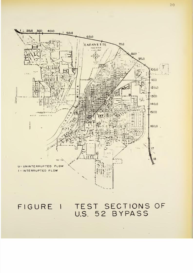
The
bypass
was
divided
into 18
homogeneous
study
sections
by considering
geometry,
speed limit, roadside
development, and
location
of traffic
signals.
These
sections
are shown
in
Figure
1.
Signalized
intersections
8/11/2019 Speed Delay
http://slidepdf.com/reader/full/speed-delay 34/141
20
i
2(U)
311)
4(U)
J
Oh
13(1)
I*
p.<
j|tlafiJ-|'Hl
I
IJJLJULJ I6(U)
$.7
—
-;
rosf
r\
sA^SOL
IKI)
i2(u)
14(U)
U-
UNINTERRUPTED
FLOW
\
I
=
INTERRUPTED
FLOW
rib
tap
17
,18
FIGURE
I
TEST
SECTIONS
OF
U.S.
5
2
BYPASS

8/11/2019 Speed Delay
http://slidepdf.com/reader/full/speed-delay 35/141
21
were
separated
fro™
the
other
sections
of
thi
t
These
intersect
ions,
which wore
categorized
as
int
w,
represented
a special conditio
required
to stop
for
the
red-signal
indication.
of
'
ach
side of the
center
j
r
U
v/as
established to
define
the
zonn
of
1
of
th
traffic
signal.
I
the light changed and the
driver
was
required
to
stop,
allowance
was
made
for
a
reasonaV
comfortable
stop
within
this distance for
uncongested
coni
-
tions.
This distance was
also
sufficient
for
a
vehicle
to i
fsume
a
normal
operating speed.
Sections
3,
8, 11,
13,
and
15
were
classified
in this category of interrupted
flow.
The
signal in
Section
3
was semi
-actuated, and the
other
four
signals had fixed-time
cycles.
The
remain:
portion
of the two-lane
by
t ass
was
designated
and analyzed
as uninterrut
ted
flow.
This
category
included
Sections
2,
4,
5,
6, 7,
9,
10,
12,
14,
and
1C.
The
remaining
three
unique sections of the bypass
were
not
included in the
multivariate
analyses
of
the
interrupted
and the
uninterrupted
flows.
Sections
1 and
17
included
transitions
from
a
four-lane, divided
highway to
a
two-
lane
roadway:
Section
18
was entirely
a
four-lane
facility.
A
required
stop for all southbound
traffic
turning
left
onto
the bypass occurred in Section l,and
traffic signals
were
present
in
Sections 17
and
18.
Drawings of
all
sec-
tions
are
presented in
Appendix
A.

8/11/2019 Speed Delay
http://slidepdf.com/reader/full/speed-delay 36/141
2?
The
selection
of the variables
to
be included
in
the
multivariate
analyses
was
dependent
on
an examination
those
variables included
in previous
investigations
and
on
the
availability
and
ease
of
collecting
dat^.
The
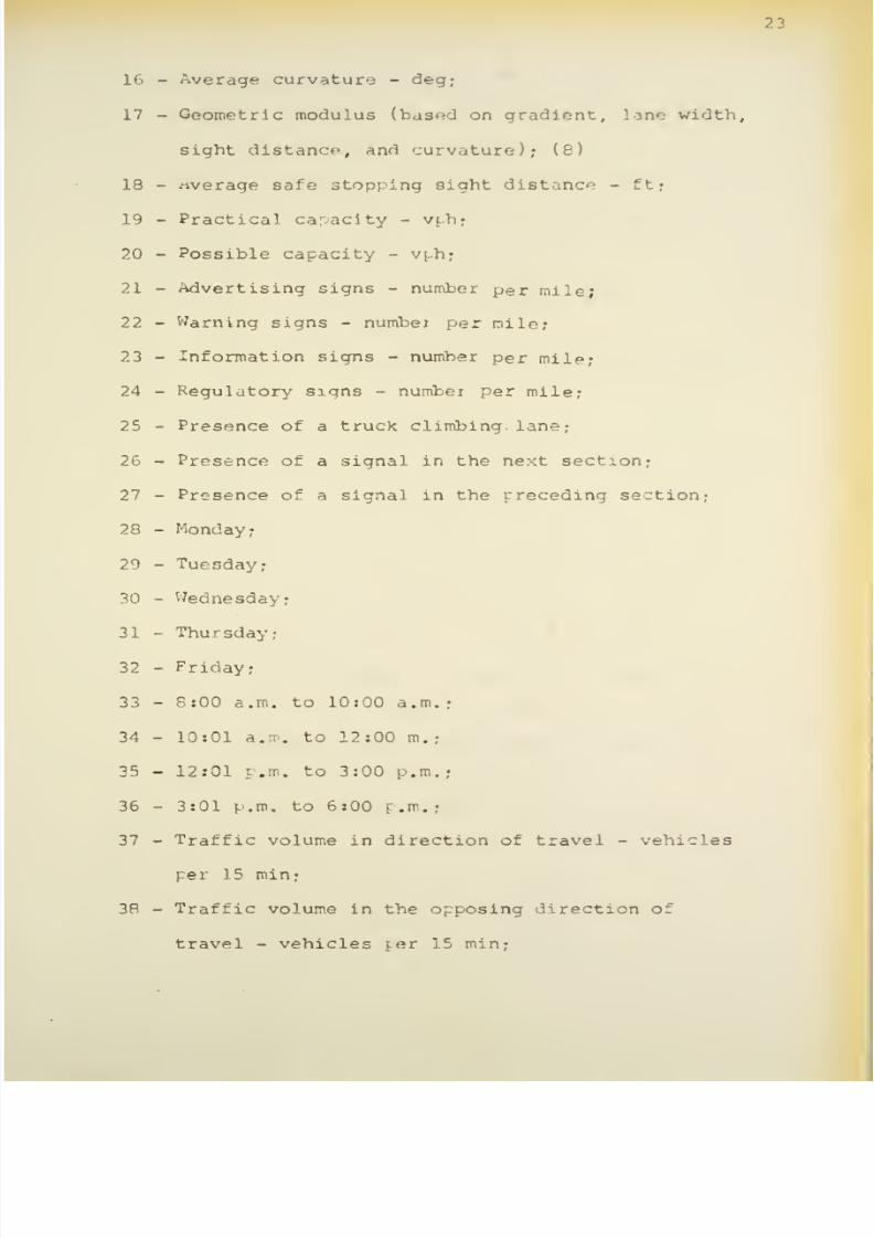
following variables
were included
in the analysis
or
unin-
terrupted flow
by
direction of
travel:
1
-
Intersecting
streets on
the right
-
number
per
mile?
2
-
Intersecting
streets on the left
-
number
ter
mile?
3
-
Intersecting
streets on
both sides
-
number per
mile
4
-
Access
drives
on
the
right
-
number
per
mile:
5
-
Access
drives
on
the
left
-
number per
mile*
6
-
Access
drives
on both sides
-
number
per
mile;
7
-
Commercial
establishments on the
right
-
number
per
mile?
8
-
Commercial
establishments
on
the
left
-
number
per
mile
•
9
-
Commercial
estahlishments
on
both
sides
-
number
per
mile;
10
-
Posted speed
limit
-
rnrh;
11
-
Average
shoulder
width
on
the
right
-
ft;
12
-
Average shoulder width
on the
left
-
ft;
13
-
Portion of section length
where passing
was not
permitted
-
percent;
14
-
Average
absolute
grade
-
percent;
15
-
Average
algebraic grade
•
signed
percent;
8/11/2019 Speed Delay
http://slidepdf.com/reader/full/speed-delay 37/141
23
16
-
Average curvature
-
deg;
17
-
Geometric
modulus
(based
on gradient, lane
width,
sight
distance,
anci
curvature);
(6)
18
-
average safe
stopping
sight
distance
-
ftj
19
-
Practical capacity
-
vphj
20
-
Possible
capacity
-
vph;
21
-
Advertising
signs
-
number
p
e
r
mile;
22
-
Warning
signs
-
number
per
mile;
23
-
Information signs
-
number
per
mile;
24
-
Regulatory
signs
-
number
per
mile;
25
-
Presence
of a
truck
climbing.
lane
26
-
Presence of
a
signal in the
next
section;
27
-
Presence
of
a
signal
in
the
preceding
section?
28
-
Monday;
29
-
Tuesday;
30
-
Wednesday;
31
-
Thursday;
32
-
Friday;
33
-
8:00
a.m.
to
10:00
a.m.;
34
-
10:01
a.m.
to
12:00
m.
35
-
12:01
p.m.
to
3:00 p.m.;
36
-
3:01 p.m.
to
6:00
p.m.;
37
-
Traffic volume
in direction of
travel
-
vehicles
per
15
min;
38
-
Traffic
volume
in
the opposing direction
of
travel
-
vehicles
jer
15 min;

8/11/2019 Speed Delay
http://slidepdf.com/reader/full/speed-delay 38/141
24
39
-
Commercial vehicles
(larger
than
a small pickup
truck)
-
percent;
40
-
Southeast direction
of travel?
41
-
Northwest
direction
of
travel;
42
-
Total traffic volume
-
vehicles
per 15
mini
43
-
Volume
to
practical capacity
ratio;
44
-
Volume
to
possible capacity ratio;
and
45
-
Overall
travel
speed
-
mph.
The
remaining
variables
were included
in the
analysis
of
interrupted
flow:
46
-
Presence
of
a
semi
-actuated signal;
47
-
Presence of
a
special
signal
for
left-turn movement;
48
-
Presence
of
a
special
right-turn lane;
49
-
Length
of approach to
special
turning
lane
-
ft;
50
-
Length
of
exit for special
merging
lane
-
ft;
51
-
Average
algebraic
grade of
approach
-
percent;
52
-
Average algebraic
grade of
exit
-
percent;
53
-
Intersecting
streets,
excluding
that
street
with
the
signal,
on
the
right
-
number;
54
-
Intersecting
streets,
excluding
that street
with
the signal, on the
left
-
number;
55
-
Intersecting streets, excluding
those
streets
with
the signal,
on
both sides
-
number;
56
-
Access
drives
on the
right
-
number;
57
-
Access
drives
on
the left
-
number;
58
-
Access
drives
on
both
sides
-
number;

8/11/2019 Speed Delay
http://slidepdf.com/reader/full/speed-delay 39/141
25
59
-
Commercial
establishments
on
the
right
-
number;
60
-
Commercial
establishments
on
the
left
-
number*
61
-
Commercial
establishments
on
both sides
-
number?
62
-
Cycle
length
of
traffic
signal
-
sec per cycle;
63
-
Green time
in direction
of flow
-
sec
per
cycle;
64
-
Practical
approach capacity
-
vj-h;
65
-
Advertising
signs
-
number;
66
-
Warning
signs
-
number;
67
-
Information
signs
-
number;
68
-
Regulatory
signs
-
number;
69
-
Southeast
direction
of
flow;
70
-
Northwest
direction of flow*
71
-
Vehicles
making
left
turns
from the direction
of
travel
-
percent;
72
-
Vehicles making
right
turns
from
the
direction
of
travel
-
percent?
73
-
Vehicles
making left
turns
from
the
opposing
direction
of travel
-
percent;
74
-
Average
shoulder
width
on
the
right
-
ft;
75
-
Average
shoulder width on the
left
-
ft;
76
-
Monday;
77
-
Tuesday;
78
-
Wednesday;
79
-
Thursday;
80
-
Friday*
81
-
8:00
a.m.
to
10:00
a.m.;
8/11/2019 Speed Delay
http://slidepdf.com/reader/full/speed-delay 40/141
26
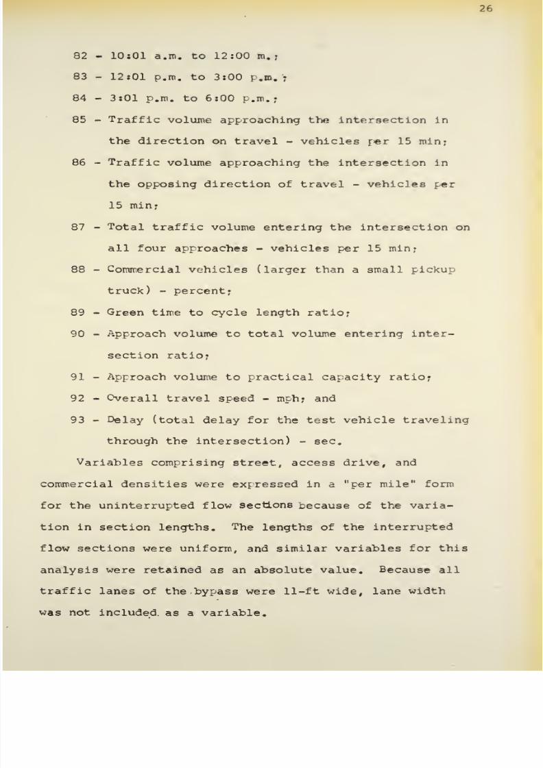
82
-
10x01
a.m.
to 12:00 m.
83
-
12:01
p.m.
to
3:00
p.m.;
84
-
3:01 p.m. to 6:00
P.m.;
85
-
Traffic
volume
approaching
the
intersection
in
the
direction
on
travel
-
vehicles per 15
min;
86
-
Traffic
volume
approaching the intersection in
the
opposing
direction
of travel
-
vehicles
per
15 min;
87
-
Total
traffic
volume entering the intersection on
all four approaches
-
vehicles
per 15
min;
88
-
Commercial
vehicles
(larger than
a small
pickup
truck)
-
percent?
89
-
Green
time
to
cycle length ratio;
90
-
Approach
volume
to
total
volume entering
inter-
section
ratio;
91
-
Approach volume
to
practical capacity ratio;
92
-
Overall
travel speed
-
inch;
and
93
-
Delay
(total
delay
for
the
test
vehicle
traveling
through
the
intersection)
-
sec.
Variables
comprising street, access
drive, and
commercial densities
were
expressed in
a
per
mile*
1
form
for the
uninterrupted flow
sections
because
of the
varia-
tion in section
lengths.
The
lengths of
the
interrupted
flow
sections were uniform,
and
similar
variables
for
this
analysis
were
retained
as an absolute
value.
Because
all
traffic
lanes
of the
bypass
were
11-ft wide,
lane
width
was not
included
as
a
variable.
8/11/2019 Speed Delay
http://slidepdf.com/reader/full/speed-delay 41/141
27
Collection
of
Data
Many
variables
in both
analyses
described the
physical
characteristics,
and
these values
remained
constant
for
each
test section.
The exceptions
were those
variables
associated with
volumes,
commercial vehicles,
time
periods,
days
of
the week, travel
speeds,
and delays.
An
inventory of
the physical
characteristics for
the
bypass
was
made from
construction plans
and
aerial photo-
graphs.
In some
cases, actual measurements
were performed
in the
field.
Section
lengths measured
by
a
fifth-wheel
odometer
were
checked with
the
control
points
located on
the construction
plans.
Possible
and
practical
capacities
were computed
in
accordance
with
methods described
in
the
Highway
Capacity
Manual
.
(11)
A
special procedure
was devised
for
computing
capacities of
the
signalized
intersections.
All
of
the
intersection? had turning
lanes on the
right
side for
both directions
of
travel.
In
only one
case, however,
was
the turning lane designated for
a
specific movement.
Drivers
used
the
added
lanes for
making
right
turns
and
for
passing
vehicles waiting
to
make
left-hand
turns.
The
additional
lane
was not fully
effective
as a
special
turning lane
in
increasing
the
approach capacity.
Capacities
were
first
computed
for the through lane.
In
addition,
the
capacities
of
the
added
turning
lane
were
8/11/2019 Speed Delay
http://slidepdf.com/reader/full/speed-delay 42/141
28
calculated for
the following
conditions:
1.
If
the predominant turning movement
was
to the
right,
the
added lane was considered
as
a right-
turn
lane; or
2.
If
the predominant turning movement was to
the
left,
the
center
lane was
considered
as
a
special
left-
turn
lane,
and
the added
lane
on the
right
was
assumed
to
handle through
and
right-turn move-
ments.
Capacities were observed
at
a
selected
intersection by
counting the number of
vehicles
passing through the
traffic
signal
during loaded green
cycles. In
a
loaded
cycle
there
was
always
a
vehicle waiting
to
enter the intersection.
The
observed capacities
were
approximately one-third of the
computed
capacities
of
the special
turning
lanes.
Therefore,
all
capacities
of
the added turning lanes
were considered
as
one-third
of
the
amount
calculated from the
Highway
Capacity
Manual
.
(11)
Volumes were recorded simultaneously
with
the measure-
ment of
travel times.
Counts were
taken
at
four
points
for
15-min
intervals.
The
control
stations,
located in Sections
2,
6,
10,
and
16,
were used
to expand the
volumes
by hour
and
by direction for
the remaining sections. All
volumes
were obtained with
recording
counters actuated by pneumatic
hoses.
The result
of
a
traffic composition
analysis
at
repre-
sentative sections
was
that the percentage
of
vehicles
8/11/2019 Speed Delay
http://slidepdf.com/reader/full/speed-delay 43/141
29
larger than a
small two-axle
pickup
truck was constant
for
all
sections
of
the bypass. Hourly fluctuations
did
occur,
and
ratios
were
established
for
different
periods
of the day.
The
percentages
of
vehicles
turning
right
and
left
at a
given
signalized intersection did
not vary
signifi-
cantly for
different
periods of
the day.
Average
values for
all types
of
turning
movements included
in
the
analysis
were
established for
each intersection.
Travel
times were
measured by the average-car
technique.
This
method was
especially
appropriate,
because
the heavy
traffic
volumes
permitted
few
opportunities
for
passing
maneuvers.
The
driver
operated
the
test
car
at a speed
which
in
his
opinion
was
representative
of the
average
speed
of
the traffic stream.
During
periods
when the test car
was
not
influenced
by
other
vehicles,
the
driver observed
the speed limit.
Travel
times at the section
boundaries
were
recorded
with
a
stop watch by
an
observer
in the
car.
Whenever
the
vehicle
was
forced
to
stop, the
duration
of
this stop
was
measured
with
a
second
stop
watch.
Forty
runs
were
made
in each direction
to assure
a
good
estimate
of
the mean
travel
speed for
each
section.
(1,19)
This
procedure
provided
a
sample
size
of
800
observations
for
the ten sections representing
uninterrupted
flow.
Five
sections provided
a
sample
size
of
400
observa-
tions for the
analysis of
interrupted
flow.
All test
car
runs
were made
over
the
entire
length
of
the bypass.
The
test vehicle entered the
traffic
stream

8/11/2019 Speed Delay
http://slidepdf.com/reader/full/speed-delay 44/141
30
about
0.5
mile
before
the
first
section
and
continued
for
approximately
the same distance after
the last section.
The
data
collections
were
made on weekdays,
in
daylight
between
the
hours
of
8:00
a.m. and
6:00
f.m., and
during
clear
and
dry
weather
conditions.
To
insure
a
variation
in
traffic volumes,
trips were
made
during
teak
and off-peak
hour
s
Analysis
of
D*ta
Data
collected
in
this investigation
were coded, punched
on
IBM
cards,
and verified.
The
computations
were
performed
on an
IBM
7094
Computer.
In
addition
to using
programs
from
the
Statistical Laboratory
of Purdue University,
special
programs were
written
to
organize
and
summarize the data.
Preliminary
Data Processing
The
data
were
first
processed and summarized
before
the
multivariate analyses were
initiated.
A
flow
diagram
of the
procedure
is
depicted
in
Figure
2.
Travel
times for
each
run and
section
were
converted
to
overall
travel
speeds
as
follows
2
s
.
L
(3600)
'•
~
T
where
S
=
overall
travel speed, mph,
L =
length
of test section,
miles,
and
T
=
travel
time, sec.

8/11/2019 Speed Delay
http://slidepdf.com/reader/full/speed-delay 45/141
31
OBSERVED
DATA
PUNCH
TRAVEL TIMES
ON
CARDS
AND
VERIFY
COMPUTE
TRAVEL
SPEEDS,
DELAYS,
AND
SUMMARIZE
RESULTS
PUNCH DATA
FOR
MULT I
-
VARIATE
ANALYSIS
ON
CARDS
AND
VERIFY
CORRELATION
ANALYSIS
1
DELETE
VARIABLES
TO
AVOID
SINGULARITY
CALCULATE
INTERSECTION
DELAYS
BY
THEORETICAL
METHOD
AND
COMPARE
WITH OBSERVED DATA
MULTIPLE LINEAR
REGRESSION
ANALYSIS
(
A
J
FACTOR
ANALYSIS
©
FIGURE
2
FLOW
DIAGRAM
FOR
DATA
PROCESSING
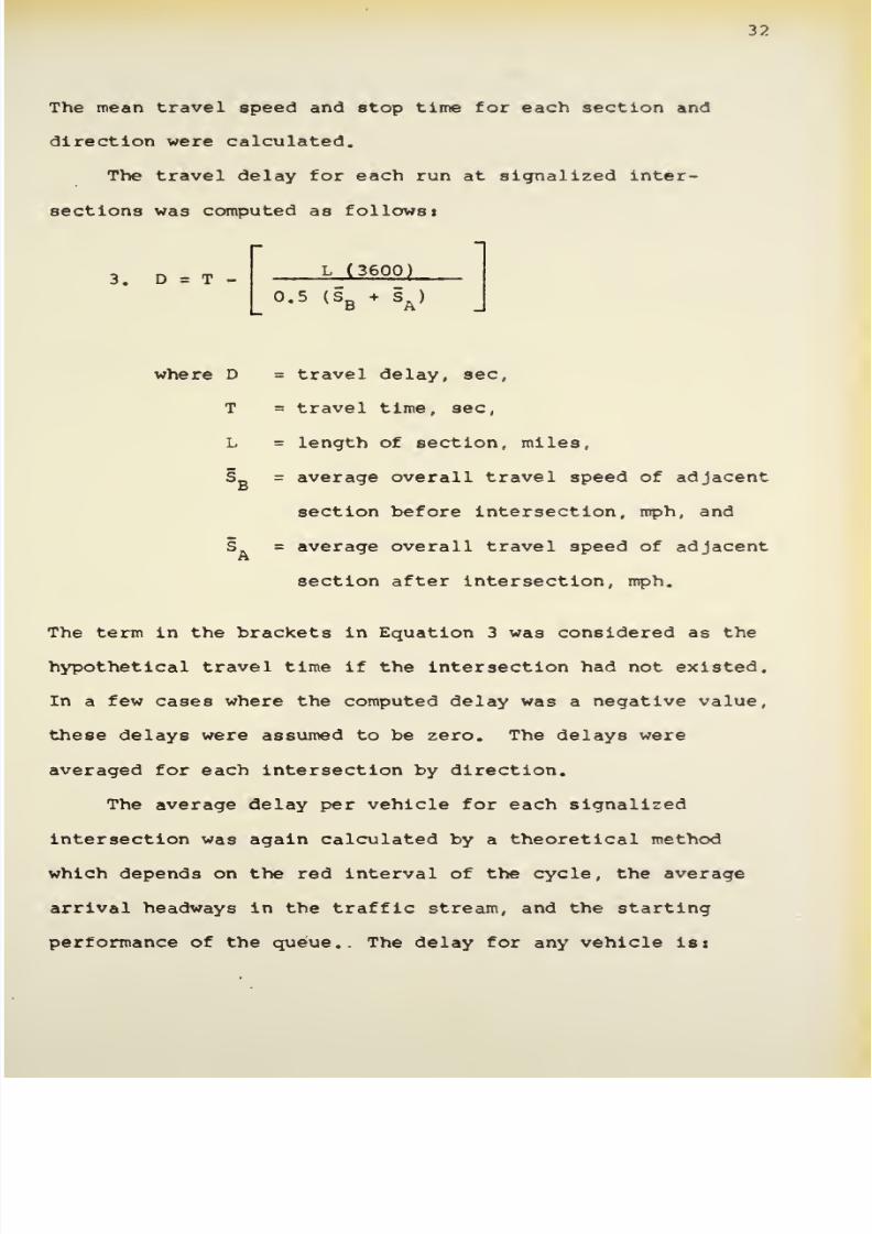
8/11/2019 Speed Delay
http://slidepdf.com/reader/full/speed-delay 46/141
32
The
mean
travel speed
and
atop time
for
each
section
and
direction were calculated.
The
travel delay
for each
run
at
signalized
inter-
sections
was
computed
as
follows
3.
D
=
T
-
L
(3600)
0.5
(S
B
*
S
A
)
where
D
=
travel
delay,
sec,
T
=
travel
time,
sec,
L
=
length
of section,
miles,
S_
=
average
overall travel
speed of
adjacent
section
before
intersection,
mph,
and
S
=
average overall travel
speed
of adjacent
section
after intersection,
mph.
The
term
in the
brackets in
Equation
3
was considered as the
hypothetical
travel
time if the intersection
had
not
existed.
In
a
few
cases
where
the computed delay was
a
negative
value,
these delays
were assumed to be zero.
The
delays
were
averaged for
each
intersection by direction.
The
average
delay
per
vehicle
for
each
signalized
intersection was
again
calculated by
a
theoretical
method
which
depends
on
the red
interval
of the cycle,
the average
arrival headways
in
the traffic stream, and the starting
performance
of the
queue. The
delay
for any
vehicle
is:

8/11/2019 Speed Delay
http://slidepdf.com/reader/full/speed-delay 47/141
33
•
a
1=R
-^l_^i
+
E
Dj
X
x=l
where
d
=
delay
for
i-th
vehicle,
sec,
R =
length
of stop
time
in
cycle,
sec,
A
=
average
arrival
headway, sec,
i
=
any
selected
vehicle,
and
D
=
headway of departure
of
x-th
vehicle,
sec.
The
total
delay
for
the
n
vehicles
stopped
in
R
is:
x=l
x=l
where
T
=
total
delay
for
all
vehicles,
sec,
and
n
=
total
number of vehicles
stopped
in
R.
The
equation
is
simf
lif ied by considering
D
as
a
constant:
6#
T
=
nR
.
h a
+
?
,
l(n)(n
*
1)
+
3#7n
_
Q
where
D
=
constant (depending
on
the
value on
n).
The number
of
vehicles
stopped
in
the red
interval
is
determined
by differentiating
T
with respect to n:
n
R
+
4.75
7
-
n
=
A
-
2 l
The
average
delay
per
vehicle
is
S.
T.§ft

8/11/2019 Speed Delay
http://slidepdf.com/reader/full/speed-delay 48/141
34
where
T
=
average
delay per
vehicle,
sec, and
C
=
cycle
length,
sec.
Complete details
of this derivation are presented in
the
textbook,
Traffic
Engineering
.
(16)
Multivariate
Analyses
The
first
step
in
each multivariate
analysis
was
the
calculation
of
a
correlation
matrix
for
the
study
variables,
because certain variables
had
to
be
deleted to
avoid
singu-
larities. These variables
included
commerical
establish-
ments, access
drives,
street
intersections,
and volumes.
If
any
two
of
the three
variables
(for
example number
of
access
drives
on the
right, number
of
access drives
on the
left, and
total
number
of
access drives)
were
known,
then
the
third
value
could
be computed.
The
variable which
had
the
smallest
product-moment
correlation
with the dependent
variable
was
removed.
Factor
Analysis
.
Before
the
factor
analysis was
per-
formed,
the
dependent variables
were
deleted
from the
correlation
matrix.
This
procedure permitted later
correlations between
the
dependent
variables
and
the genera-
ted
factors.
A
flow
diagram for
the factor analysis
is
shown
in
Figure
3.
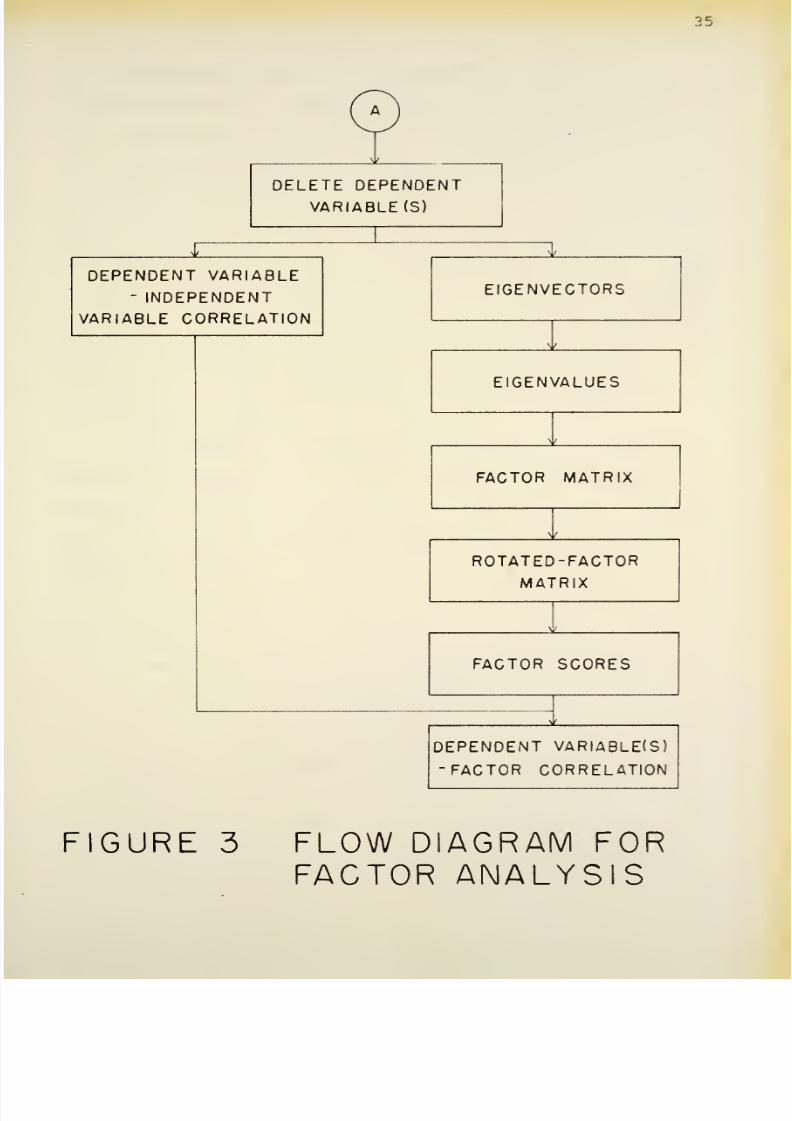
8/11/2019 Speed Delay
http://slidepdf.com/reader/full/speed-delay 49/141
25
DELETE
DEPENDENT
VARIABLE
(S)
£
DEPENDENT VARIABLE
-
INDEPENDENT
VARIABLE CORRELATION
EIGENVECTORS
*
EIGENVALUES
v
FACTOR
MATRIX
1
v
ROTATED-FACTOR
MATRIX
V
'
FACTOR
SCORES
3
DEPENDENT
VARIABLE(S)
-FACTOR
CORRELATION
FIGURE
3
FLOW
DIAGRAM FOR
FACTOR
ANALYSIS

8/11/2019 Speed Delay
http://slidepdf.com/reader/full/speed-delay 50/141
36
Orthogonal
factors
were
generated so
that
a
maximum
contribution
to
the
residual
communality was
provided.
(
20,
31)
The
generation of
the factors
was
terminated
when
the
eigenvalue became
less
than
1.00.
It
has
been
arbitrarily
established that factors with
eigenvalues
of
1.00
contribute
significantly
to
the total
variance
of
the variables.
(18)
The
factor matrix
was
thus
established,
which
contained
less
elements
than
the original
correlation
matrix.
This
factor
matrix was
rotated
with
the
varimax method
to aid
interpre-
tation of each
factor.
(20,
31) An
examination
of
the
rotated-factor matrix resulted
in
the
identif
iciation of
the
generated factors.
Coefficients
were
developed
to express
each factor
in
terms
of
the original
variables.
Thus,
the
factors
were
evaluated
from
the
values
of
the
variables
that
were
signifi-
cantly
related
to
each factor.
These
factor
scores
were
computed
as
follows:
9.
E =
FA'Y~
2
A
where
E
=
factor-score
matrix,
F
=
rotated-factor
matrix,
A =
factor
matrix,
and
Y
=
diagonal
matrix
of
eigenvalues. (18)
The
final
step
in
the
factor
analysis
was the
correlation
of
the
factors
with the dependent
variables.
The
resulting multiple
linear
regression
equation
expressed

8/11/2019 Speed Delay
http://slidepdf.com/reader/full/speed-delay 51/141
37
the
dependent
variable
as
a
function
of
the significant
factors.
The
regression
coefficients
were
calculated from
the
following
matrix equation:
10.
c
=
Er'
where
c
=
column vector
of
regression coefficients,
E
=
factor-score matrix, and
r
=
row
vector
of correlation
coefficients
for dependent
variables correlated
with
other variables.
(18)
Multiple
Linear
Regression
and
Correlation
Analysis.
A
build
up
regression analysis
was performed on the study
variables.
(32)
A
flow
diagram
for
this procedure is
shown
in
Figure
4.
At
each
step
in
the
routine,
a
F-to-remove
value was
computed
for
each
variable in the
regression
equation,
and
F-to-enter
values
were computed for
the
variables
not
in
th« equation.
Independent variables
were
deleted
and added
under
the
following conditions
1.
If
in
the
regresson equation
there
were
one or
more
independent
variables
which
had
an
F
value
less than the critical
M
F-to-remove value
speci-
fied,
the
variable
with
the smallest
F
value was
removed
y
2.
If
no
variable was removed and there
were
one
or
more
independent
variables,
not
in
the
regression

8/11/2019 Speed Delay
http://slidepdf.com/reader/full/speed-delay 52/141
38
B
COMPUTE
REGRESSION
EQUATION
COMPUTE
F
TO REMOVE
VALUE
FOR
EACH
VARIABLE IN EQUATION
>F
CRITICAL
^L
COMPUTE F TO ENTER
VALUE
FOR
EACH
VARI
-
ABLE NOT
IN EQUATION
<FCRITICAL
TERMINATE PROCEDURE
<
F
CRITICAL
DELETE
VARIABLE
>F
CRITICAL
ENTER
VARIABLE
FIGURE
4 FLOW
DIAGRAM
FOR
MULTIPLE
LINEAR
REGRESSION
ANALYSIS
8/11/2019 Speed Delay
http://slidepdf.com/reader/full/speed-delay 53/141
39
equation, which
passed
a
tolerance test,
the
variable
with the highest
F
value was added*
and
3.
If
no
variable was added
or
deleted, the procedure
was
terminated. (20)
Values of
0.01
and
0.005
were
specified
as
F-levels
for
inclusion
and
deletion, respectively.
The
variables
were
assigned
numerical ratings.
Those
variables
with the lowest
rating
were considered
first
for
deletion?
likewise,
the
vari-
ables
with
the
highest
rating
were considered
initially
for
entrance
into
the
equation.
The
procedure
was
repeated
for
the
variables
with
the
next-to-lowest
and
next-to-highest
ratings considered for
exit
and
entrance,
respectively,
until
the program was
terminated. These ratings affected
only
the
order of adding and
removing
the
study
variables,
and
the
regression
coefficients were
not
altered
in
magnitude
or
sign.
(20)
The
following criteria were
used in rating
the
vari-
ables for inclusion
in
the
multiple
linear
regression
equa-
tions:
1.
Each
significant factor
was
represented
by
at
least one closely related
variable*
2.
The
final model
involved
a
minimum of computations
with readily obtainable
data;
and
3.
The
multiple coefficient
of determination did not
increase significantly by including additional
variables.

8/11/2019 Speed Delay
http://slidepdf.com/reader/full/speed-delay 54/141
40
Mathematical
Models
The
development
of
functional relationships
between
the dependent variables and
the
factors and
independent
variables involved
the formulation
of
mathematical models,
These
statistical models
provide
a
basis of
formulating
theories
in
traffic flow.
The
types of
multiple
linear
regression
equations used
in
the
analysis
weret
11.
Y
1
=
Y
+
y
(cjFj
+
c
2
F
2
+
. .
.
c
F
where
Y
=
predicted
mean
dependent
variable,
Y
=
grand
mean
of
dependent
variable,
y
=
standard deviation of
dependent
variable,
c
=
common factor
coefficient,
F
=
common
factor,
and
q
=
number
of
common factors.
12.
Y
=
a
+
b.X
+
b_X
+
.
.
.
+
b
X
2
112
2
p
p
where
Y
=
predicted mean dependent
variable,
a
=
intercept,
b
=
regression
coefficient,
X =
independent variable,
and
p
=
number
of independent
variables.
These
multiple
linear
regression
equations
were developed
assuming
that
the
sample
data
were
randomly
selected
from
normal
populations.
Also,
homogeneity
of
variance
was
8/11/2019 Speed Delay
http://slidepdf.com/reader/full/speed-delay 55/141
41
RESULTS
The
results
of
the
multivariate
analyses of
travel
speeds and delays
are
presented
and
discussed
in this
section.
The
data
were
first
summarized by computing
mean
travel speeds
and delays
for
each
study section.
A
factor
analysis was
performed to
gain
an
insight
into the
relation-
ships
among
the
study variables.
Multiple
linear regres-
sion equations were
developed to
predict mean travel
speeds
and delays
in
terms of the
factors
and the
variables.
The
results of these
analyses
were
then
applied in
recommending
improvements
to
minimize
delays on
the
bypass
location.
All
variables
were
identified
by
the numbers
which
are
listed
in
the
discussion
of
the experimental
design.
Each
factor
was labeled
with
a
letter
in
the
evaluation of
the
results
of the
factor
analysis.
Uninterrupted
Flow
The
overall travel
speeds for each
test
section
in
the analysis
of
uninterrupted flow were
averaged for
both
directional flows
and the combined flows.
These
mean travel
speeds
are
summarized
in
Table
1.
The
highest speeds
occurred
in Sections
5,
6,
and
7 where the commerical
roadside

8/11/2019 Speed Delay
http://slidepdf.com/reader/full/speed-delay 56/141
TABLE
1
AVERAGE
OVERALL
TRAVEL
SPEEDS,
UNINTERRUPTED
FLOW
42
Section
Average
Overall
Travel
Speed,
mph
SE Flow
NW
Flow
Combined
Flow3
2
41.4
40.6
41.0
4
42.0
47.7
44.9
5
51.0
52.5
51.8
6
52.8
53.9
53.4
7
45.1
45.2
45.2
9
40.3
42.0
41.2
10
40.8
42.6
41.7
12
34.4
39.3
36.9
14
30.4
33.5
32.0
16
35.3 35.3 35.3

8/11/2019 Speed Delay
http://slidepdf.com/reader/full/speed-delay 57/141
43
development
was sparse.
In
Sections
12, 14,
16
where
heavy
commercial
strip
development
occurred,
the
lowest
speeds
were
recorded.
Factor
Analysis
A
correlation matrix
was
calculated for
variables
1
to
45
inclusive.
The
correlation
of
travel
speed
with the
other
variables
is
presented
in
Table
14,
Appendix
B.
Variables
2,
5,
8,
and
38
were deleted from
the
matrix
to
avoid
singularities.
Variables
40
and
41,
which
identified
the
directional flows,
and
variable
45,
overall travel
speed,
were
also
removed.
This
speed variable
was
later
correlated
with
the generated factors.
The
revised correlation matrix
was
factorized with
unities
inserted
in
the main
diagonal
of the
matrix.
The
38 variables were reduced
to
13
factors
which accounted
for
88
percent of
the
total variance of the
variables.
The
eigenvalue
and the
portion of
variation
explained
by
each factor
are shown
in
Table
15,
Appendix
B.
The
13 factors were then
rotated to
aid
in
their
identi-
fication.
This rotated-f
actor
matrix
is
presented
in
Table
2,
The
signed factor coefficients
indicate
the
relative
importance of each
variable in the explanation of
the
generated
factors.
The
plus
and
minus signs are indicative,
respectively,
of the
increasing
or
decreasing
presence
of
the variables
in
the
composition
of
the
factors. Each
factor

8/11/2019 Speed Delay
http://slidepdf.com/reader/full/speed-delay 58/141
TABLE
2
ROTATED-FACTOR
MATRIX,
UNINTERRUPTED
FLOW
44
Vari-
able
Factors
A
B
C
D
E
F
1
-0.0056
+0.3019 +0.0136
+0.1050
+0.0222
+0.8397
3 -0.1582
+0.3942
-0.0119
+0.0404
-0.0071 +0.7510
4
+0.9290
-0.1625
+0.0069
-0.0207 -0.0020 +0.0790
6
+0.9294
-0
.
1 848
+0.0079
-0.0088
+0.0006
-0.0676
7 +0.9176 -0.1792
+0.0054
-0.0354
-0.CO62 +0.0188
9
+0.9287
-0.2071 +0.0079
-0.0119 -0.0021 -0.1201
10
-0.49
30
-0.1115 -0.0062
+0.0555 +0.0011 -0.4368
11
+0.2341 +0.0806 +0.0101
+0.1530
-0.0035 +0.1327
12 +0.5259 +0.0973
+0.0108
-0.2712
-0.0112 +0.5798
13
-0.0929
+0.9244
-0.0273 -0.0062
-0.0115
+0.1711
14
-0.3658
+0.1278
+0.0171
-0.1663
+0.0404
-0.2513
15 +0.0152 +0.0130 -0.0093 -0.9151
-0.0134 +0.0981
16
-0.0560
+0.7644 -0.0101
-0.0366
+0.0009
+0.1718
17
+0.2464 -0.869
3
+0.0228
+0.0199
+0.0175
-0.1567
18
+0.1329
-0.744
3
+0.0312
-0.0305
+0.0457
-0.2903
19
+0.4734
-0.7638
+0.0404
-0.0406 +0.0224 +0.1154
20
-0.0910 -0.7556
+0.0412
-0.1030 +0.0424
-0.1330
21
+0.0862 +0.2952 +0.0013
+0.1395
+0.0143
+0.2244
22 +0.2828 +0.1170 +0.0064
-C.6533
+0.0102 -0.2374
23
-0.1591
+0.0204
-0.0179
-0.1585
-0.0260 -0.2668
24 +0.1862
-0.4398
+0.0198
-0.0983
+0.0126
+0.4697
25
-0.1380
-0.2072
+0.0134
-0.6860 +0.0231
-0.0665
26
+0.4114
+0.0460 +0.0034
-0.3607
-0.0081
-0.0014
27
+0.5888
+0.1605
-0.0065
+0.3658
-0.0169 +0.1828
28
-0.0042 +0.0108
+0.3523
+0.0026
+0.1313
-0.0053
29
+0.0066
+0.0096
+0.1059
+0.0106 +0.1712
+0.0031
30
-0.0028 -0.0181
-0.1230
-0.0092 -0.7612
+0.0114
31
+0.0054 -0.0139 -0.6170 -0.0078 +0.4544
-0.0045
32
-0.0066
+0.0221
+0.4392
+0.0079 +0.2336
-0.0104
33
+0.0035
-0.0228
-0.2464 -0.0187 +0.1671 -0.0021
34 +0.0033 -0.0111
-0.7637 +0.0030 +0.3788
+0.0152
35
-0.0029 -0.0044 -0.0831 +0.0041
-0.8616 -0.0145
36
-0.0025
+0.0252 +0.8724 +0.0042
+0.3225
+0.0007
37
+0.4374
+0.0378 +0.4516
-0.0408
+0.2133 +0.0624
39 +0.0110
-0.0231
-0.9082
-0.0102
-0.0649
+0.0034
42
+0.4683
+0.0246
+0.4839
-0.0671 +0.2212
+0.0691
43
-0.0865
+0.8605 +0.2957 -0.0169 +0.1362
-0.07
30
44
+0.3728
+0.4906 +0.3996 -0.0408 +0.1786 +0.0933
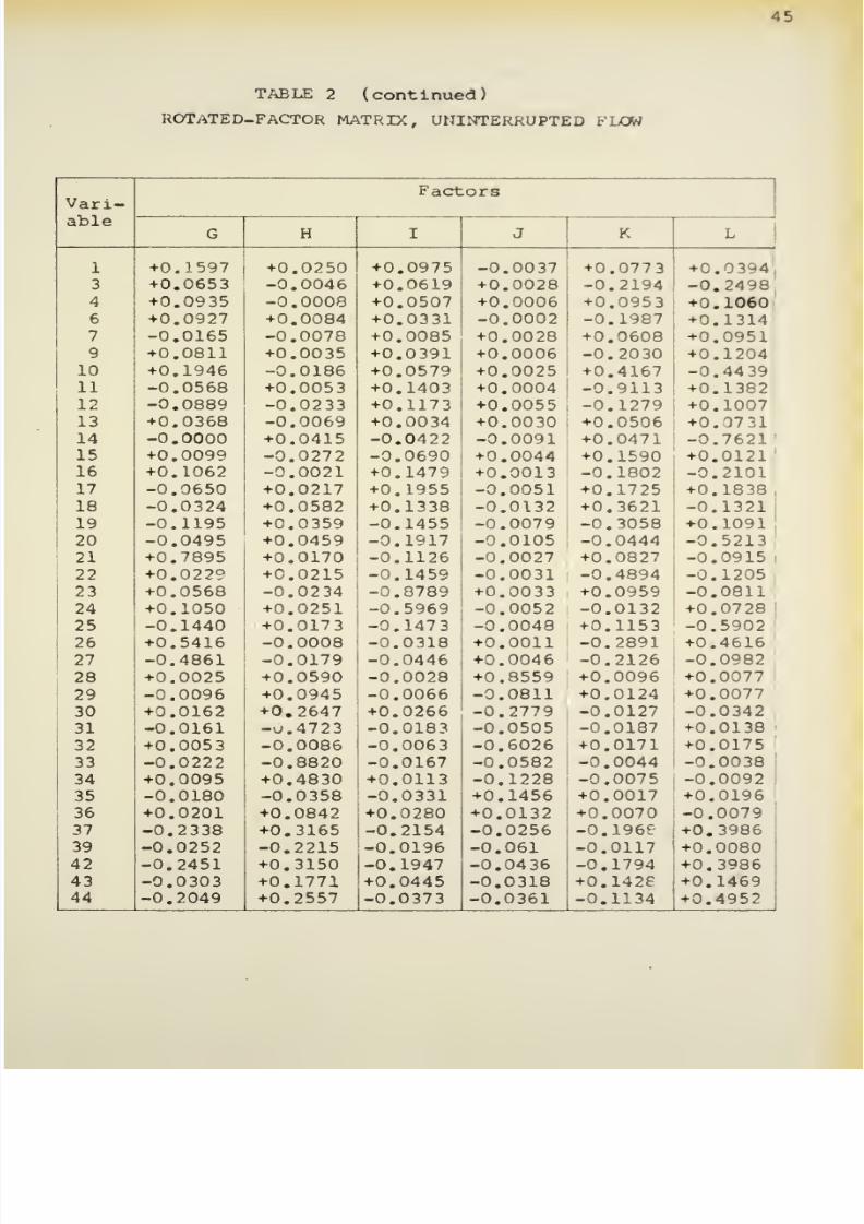
8/11/2019 Speed Delay
http://slidepdf.com/reader/full/speed-delay 59/141
TABLE
2
(continued)
ROTATED-FACTOR
MATRIX,
UNINTERRUPTED
FLOW
45
Vari-
Factors
able
G H
I
J
K
L
1
+0.1597
+0.0250
+0.0975 -0.0037 +0.0773
+0.0394
3
+0.0653 -0.0046
+0.0619
+0.0028
-0.2194
-0.2498
4
+0.0935
-0.0008
+0.0507
+0.0006 +0.0953
+0.1060
6 +0.0927 +0.0084
+0.0331
-0.0002
-0.1987
+0.1314
7
-0.0165 -0.0078
+0.0085
+0.0028 +0.0608
+0.0951
9 +0.0811
+0.0035
+0.0391
+0.0006
-0.2030
+0.1204
10
+0.1946 -0.0186
+0.0579 +0.0025
+0.4167 -0.44
39
11
-0.0568
+0.0053 +0.1403
+0.0004
-0.9113
+0.1382
12
-0.0889
-0.0233 +0.1173
+0.0055
-0.1279
+0.1007
13 +0.0368
-0.0069
+0.0034
+0.0030
+0.0506 +0.3731
14
-0.0000
+0.0415 -0.0422 -0.0091
+0.0471
-0.7621
15
+0.0099
-0.0272
-0.0690
+0.0044
+0.1590 +0.0121
16
+0.1062
-0.0021
+0.1479 +0.0013 -0.1802 -0.2101
17 -0.0650
+0.0217
+0.1955 -0.0051
+0.1725
+0.1838
18
-0.0324
+0.0582 +0.1338
-0.0132
+0.3621 -0.1321
19
-0.1195
+0.0359
-0.1455
-0.0079
-0.3058
+0.1091
20
-0.0495 +0.0459 -0.1917 -0.0105 -0.0444 -0.5213
21
+0.7895 +0.0170 -0.1126
-0.0027 +0.0827 -0.0915
22
+0.0229 +0.0215
-0.1459 -0.0031 -0.4894 -0.1205
23
+0.0568
-0.02
34
-0.8789
+0.0033 +0.0959
-0.0811
24 +0.1050
+0.0251
-0.5969
-0.0052 -0.0132 +0.0728
25
-0.1440
+0.0173
-0.147
3
-0.0048
+0.1153
-0.5902
26 +0.5416
-0.0008 -0.0318
+0.0011
-0.2891 +0.4616
27
-0.4861 -0.0179 -0.0446 +0.0046
-0.2126
-0.0982
28 +0.0025 +0.0590
-0.0028
+0.8559
+0.0096 +0.0077
29
-0.0096 +0.0945
-0.0066 -0.0811
+0.0124
+0.0077
30
+0.0162
+0.2647
+0.0266
-0.2779 -0.0127
-0.0342
31
-0.0161
-u.4723
-0.0183
-0.0505
-0.0187 +0.0138
32
+0.0053
-0.0086
-0.0063 -0.6026 +0.0171
+0.0175
33
-0.0222
-0.8820 -0.0167
-0.0582
-0.0044
-0.0038
34
+0.0095
+0.4830 +0.0113
-0.1228
-0.0075 -0.0092
35
-0.0180
-0.0358
-0.0331 +0.1456 +0.0017
+0.0196
36
+0.0201
+0.0842 +0.0280 +0.0132
+0.0070 -0.0079
37 -0.2338
+0.3165
-0.2154
-0.0256
-0.196f
+0.3986
39
-0.0252
-0.2215
-0.0196
-0.061 -0.0117
+0.0080
42
-0.2451 +0.3150
-0.1947
-0.04
36
-0.1794
+0.3986
43
-0.0303
+0.1771 +0.0445
-0.0318
+0.1428
+0.1469
44
-0.2049
+0.2557
-0.0373 -0.0361
-0.1134
+0.4952
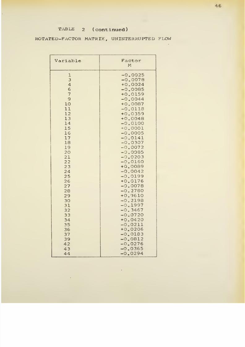
8/11/2019 Speed Delay
http://slidepdf.com/reader/full/speed-delay 60/141
46
TABLE
2
(continued)
ROTATED-F
ACTOR
MATRIX, UNINTERRUPTED
FLOW
Variable
Factor
M
1
-0.0025
3
-0.0078
4
+0.0024
6 -0.0085
7 +0.0159
9
-0.0044
10
+0.0087
11
-0.0118
12 +0.0359
13
+0.0048
14
-0.0100
15
+0.0001
16
-0.0005
17
-0.0141
18
-0.0307
19
-0.0072
20
-0.0085
21
-0.0203
22
-0.0160
23
+0.0089
24
-0.0042
25
-0.0199
26
+0.0176
27
-0.0078
28
-0.2780
29
+0.9610
30
-0.2198
31
-0.1997
32
-0.3467
33
-0.0720
34
+0.04 20
35
-0.0211
36
+0.0206
37
-0.0183
39
-0.0812
42
-0.0276
43
-0.0365
44
-0.0294
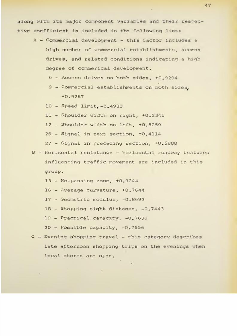
8/11/2019 Speed Delay
http://slidepdf.com/reader/full/speed-delay 61/141
47
along
with
its
major
component
variables
and their
resrec-
tive
coefficient
is
included in
the following
list;
A
-
Commercial
development
-
this factor
includes
a
high
number
of
commercial establishments,
access
drives, and
related
conditions
indicating
a
high
degree of
commerical
development.
6
-
Access
drives
on
both
sides, +0.9294
9
-
Commercial
establishments
on
both
sides.
+0.9287
10
-
Speed
limit, -0.4930
11
-
Shoulder
width
on
right,
+0.2341
12
-
Shoulder
width on left,
+0.5259
26
-
Signal
in
next
section,
+0.4114
27
-
Signal
in
preceding section,
+0.5888
B
-
Horizontal
resistance
-
horizontal
roadway features
influencing traffic
movement
are
included
in
this
group.
13
-
No-passing
zone,
+0.9244
16
-
Average
curvature, +0.7644
17
-
Geometric modulus, -0.8693
18
-
Stopping
sight distance, -0.7443
19
-
Practical
capacity,
-0.7638
20
-
Possible
capacity,
-0.7556
C -
Evening
shopping
travel
-
this category describes
late
afternoon shopping trips
on the
evenings
when
local
stores
are
open.
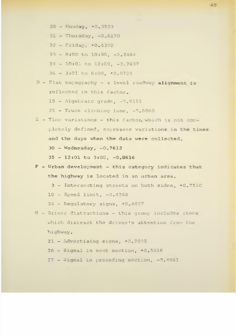
8/11/2019 Speed Delay
http://slidepdf.com/reader/full/speed-delay 62/141
48
28
-
Monday,
+0.3523
31
-
Thursday,
-0.6170
32
-
Friday,
+0.4392
33
-
8:00
to
10:00,
-0.2464
3-1 -
10:01
to
12:00,
-0.7637
36
-
3:01
to
6:00,
+0.8724
D
-
Flat
topography
-
a
level roadway
alignment
is
reflected
in
this
factor.
15
-
Algebraic
grade,
-0.9151
25
-
Truck
clinvbing
lane,
-0.6860
£
-
Time
variations
-
this
factor,
which
is
not c:
-
pletely
defined,
expresses variations
in
the
tiroes
and the
days
when
the
data
were
collected.
30
-
Wednesday,
-0.7612
35
-
12:01
to
3:00,
-0.8616
F
-
Urban
development
-
this
category
indicates that
the
highway
is
located
in an
urban
area.
3
-
Intersecting
streets
on
both sides, +0.751C
10
-
Speed
limit,
-0.4
368
24
-
Regulatory
signs,
+0.4697
G -
Driver
distractions
-
this
group
includes
iters
which
distract
the driver's attention
iron
the
highway.
21
-
Advertising
signs,
+0.78
26
-
Signal
in
next
section,
+0.5416
27
-
Signal
in
preceding
section,
-0.4861
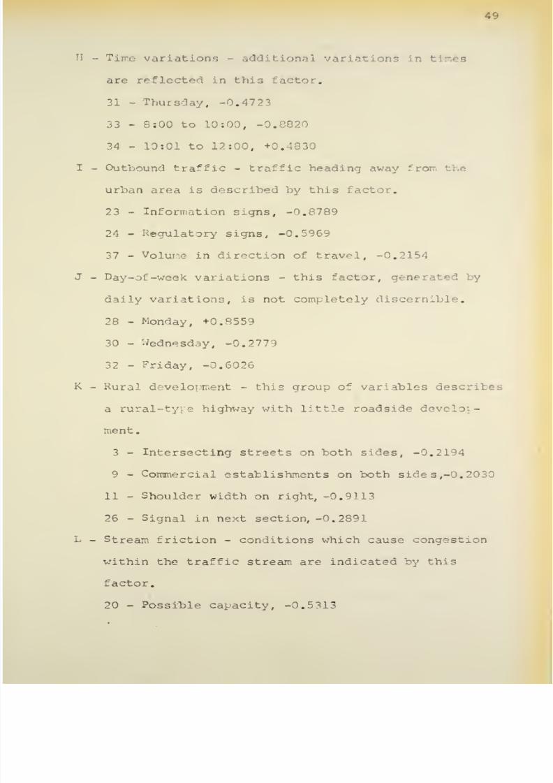
8/11/2019 Speed Delay
http://slidepdf.com/reader/full/speed-delay 63/141
49
n
-
Time
variations
-
additional
variations in
tir.es
are
reflected
in this
factor.
31
-
Thursday, -0.4723
33
-
8:00
to
10:00,
-0.8820
34
-
10:01
to
12:00,
+0.4830
I
-
Outbound traffic
-
traffic
heading
away
from the
urban area
is
described by
this factor.
23
-
Information
signs,
-0.8789
24
-
Regulatory
signs,
-0.5969
37
-
Volur.e
in direction
of
travel,
-0.2154
J
-
Day-of-week
variations
-
this
factor,
generated
by
daily
variations,
is
not completely
discernible.
28
-
Monday,
+0.8559
30
-
Wednesday,
-0.2779
32
-
Friday,
-0.6026
K
-
Rural
development
-
this
group
of
variables
describes
a
rural
-tyve
highway
with
little
roadside
develo
-
ment.
3
-
Intersecting
streets
on both sides,
-0.2194
9
-
Commercial
establishments
on
both
side
s,
-0.2030
11
-
Shoulder width
on right,
-0.9113
26
-
Signal
in
next
section,
-0.2891
L
-
Stream
friction
-
conditions
which
cause
congestion
within
the
traffic stream are
indicated
by this
factor.
20
-
Possible
capacity, -0.5313

8/11/2019 Speed Delay
http://slidepdf.com/reader/full/speed-delay 64/141
50
25
-
Truck
climbing
lane, -0.5902
26
-
Signal
in next
section,
+0.4616
37
-
Volume
in
direction
of
travel, +0.3986
44
-
Volume
to
|.ossible
capacity
ratio,
+0.4952
M
-
Day-of-week
variations
-
this
factor
reflects
further
variations
for
different
days
of
the
week.
28
-
Monday,
-0.2780
29-
Tuesday,
+0.9610
32 -
Friday, -0.3467
These
factors
were
readily
identified
except
for
those
associated with time-of-day
and day-of-week characteristics.
These
variations
resulted from the random selection
of
different
days
and time periods for conducting
the travel-
time
studies.
The
next execution in the factor-analysis procedure
was
the computation of the factor-score matrix
which
is
presented
in
Table
3.
The
coefficients
in
this
matrix
permit
the
factors
to be
evaluated
as
functions
of the
original variables
which
are
expressed
in
terms
of
multiple
linear regression equations. Exam>
les
of these equations
are presented later
in
the
results.
The
final
step was the
correlation of
each
factor
with
the mean
overall travel
speed
to determine
those fac-
tors
which
significantly
accounted for the variation in
travel
speeds.
These correlation coefficients are listed
in
Table
4.
The
four
factors which
were
significant
at
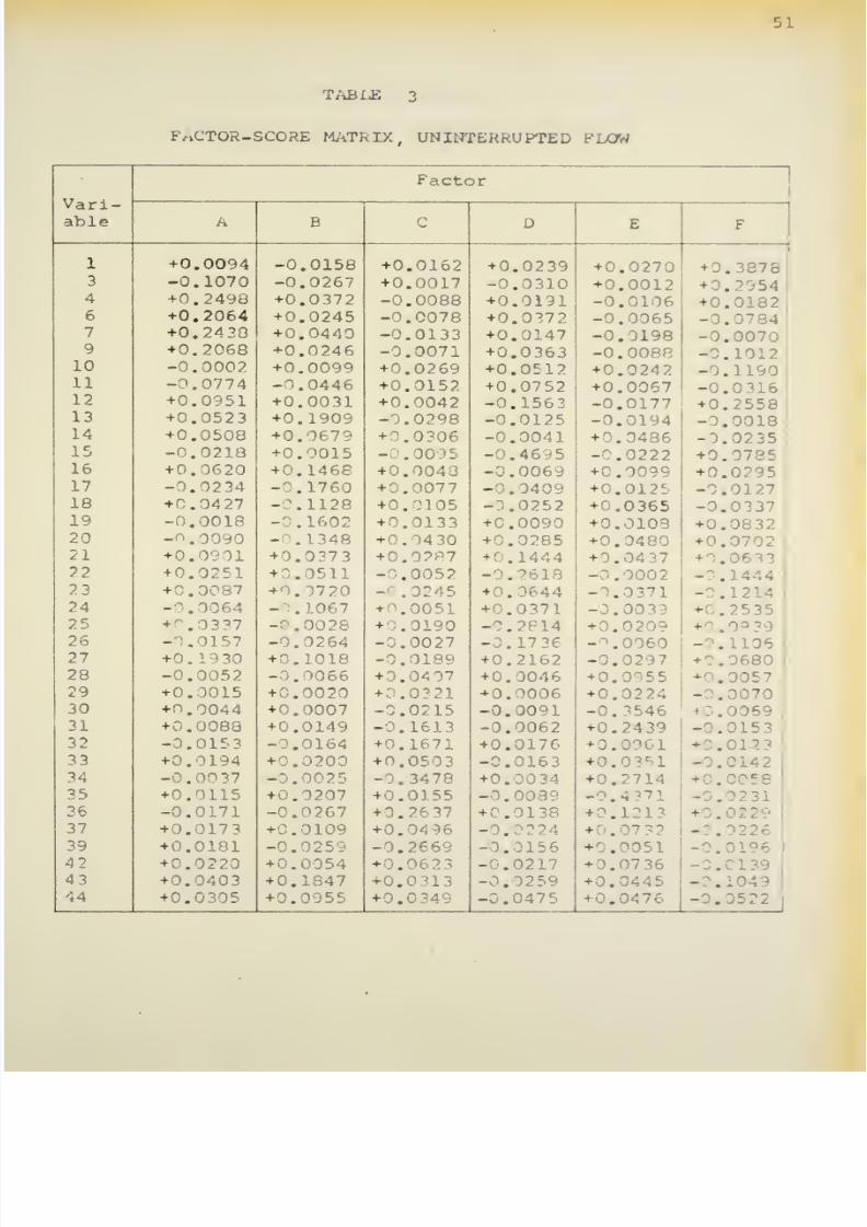
8/11/2019 Speed Delay
http://slidepdf.com/reader/full/speed-delay 65/141
TABUS
FACTOR-SCORE
MATklX,
UNINTERRUPTED
FLOW
Vari-
Factor
able
A
B
C
D
E
F
1
+0.0094
-0.0158
+0.0162
+0.0239
+0.0270
+0.387&
3
-0.1070
-0.0267
+0.0017
-0.0310
+0.0012
+0.2354
4
+0.2498
+0.0372
-0.0088
+0.0191
-0.0106
+0.0182
;
6
+0.2064
+0.0245
-0.0078
+0.0372
-0.0065
-0.0784
7
+0.2430
+0.0440
-0.0133
+0.0147
-:.3198
-3.0070
9
+0.2068
+0.0246
-0.0071
+0.0363
-0.0088
-0.1012
10
-0.0002
+0.0099
+0.0269 +0.0512 +0.0242
-3.1190
'
11
-1.0774
-0.0446
+0.0152
+0.0752
+0.0067
-0.0316
12
+0.0951
+0.0031
+0.0042
-0.1563
-0.0177
+0.2558
13
+0.0523
+0.1909
-0.0298
-0.0125
-0.0194
-
.0018
14
+0.0508
+0.0679 +^.0306
-0.0041
+0.0486
-3.0235
15
- .0218
+0.0015
-
.0005
-0.46
-
.0222
+0.0785
16
+0.0620
+0.1468
+0.0048
-0.0069
+0.0099
40.0295
17
-
.0234 -0.1760
+0.0077
-
.3409 +0.0125 -0.0127
18
+0.0427
-
.1128
+0.0105
-^.0252
+0.0365
-0.0
337
19 -0.0018
-
.1602
+0.0133
+0.0090
+0.0103
+0.0832
20
-
.0090
-
.1348
+0.04
30
+
.0285
+0.0480
+0.0702
21
+0.0901 +0.0373
+0.0287
+
.1444
+ 3. +
0.0'
22
+0.0251
+
.0511
-
.0052
-
.
>6ia
-
.0002
-
.1444
23
•
.
0087
+0.0720
-
.3245 +0.3644
-
.
)371
-
.1214
,
24
-~.1064
-
.1067
+
.0051
+0.0371
39 +
.2535
;
25
+0.0337
-
.0028
+
.0190
-0.2814
+0.0209
-
26
-
.3157
-
. )264
-
.0027
-
.1736
-0.0060
-
.1106
27
+0.1930
*
.1018
-0.0189
+0.2162
-
.029
7
-
.0680
i
28
-0.0052
-
.
166
+0.0407
+0.0046 +0.0955
-
.0057
29
+0.0015
+0.0020 +
.0321
+0.0006
+0.0224
-
.0070
30
+0.0044
+O.0007
-0.0215
-0.0091
-0.3546
•
.0069
31
+0.0088
+0.0149
-0.1613
-0.0062
+0.2439
-
.0153
32 -0.015
3
-
.0164
•
.1671
+0.01
-
.
1
6
-
.0123
33
+0.0194
+0.0200 +0.0503
-0.0163
+0,
-
.0142
34
-0.00
37
-'
.
>025
-
.
3478
+0.00
34
.2714
-
.
35 +0.0115 +
.1207
+0.0155
-0.0089
-0.4371
-
.
:3i
36
-0.0171 -0.0267
+0.2637
4
,
+
-'.1213 -
.
37
+0.017?
+0.0109
+0.04
56
-
.
24
. 7
-
.
39
+0.0181
-
.
.
-0.2669
.
j156
*
.
'51
-
.0196
42
+0.0220 +0.0054
+
.
-0.0217
-
.
36
.
139
43
+0.0403
+0.1847
+0.0313 -0.0259
+0.0445
-
.1049
44
+0.0305 +0.0955
+0.0
349
.0475
+0.0476
-0.3522
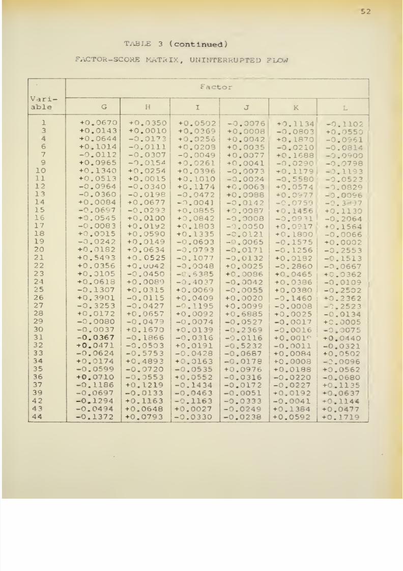
8/11/2019 Speed Delay
http://slidepdf.com/reader/full/speed-delay 66/141
TaBLE
3
(continued)
FACTOR-SCORE
MATRIX, UNINTERkUPTED
FLOW
Vari-
Factor
able
G
H
I
J K
L
1
+0.0670
+0.0350
+0.0502
-0.0076
+0.1134
-
.1102
3 +0.0143 +0.0010
+0.0369
+0.0008 -'.0803
.
4
+0.0644
-0.0173
+0.9256
+0.0042
+0.1870
-0.0961
6
+0.1014
-
i.0111
+0.0203
+0.0035
-0.0210
-0.0814
7
-0.0112
-0.0307
-0.0049
+0.0077
+0.1688
-
.
-00
9
+0.0965
-0.0154
-
.
261
+O.0041
-0.0290
-
.0798
10
+0.1340
+0.0254
+0.0396
-0.007
3
+0.1179
-
.1193
11
+0.0513
+0.0015
+0.1010
-
.0024 -0.5590
-3.0523
12 -0.0964
-0.0340
+0.1174
-
.0063
+0.0574
-
.0829
13
-0.0360
-0.0198
-0.047
2
+0.0088
+0.0977
-
.0096
14
+0.0084
+0.0677
-
.0041
-
.
-
.0759
-
.
15
-0.06
7
-0.0293
+0.0855
.
:o87
+0.1456
+0.1130
16 +
.0545 +0.0100
+
.0842
-0.0008
-0.0931
-0.2064
17
-0.008
3 +0.0192
+0.1803
-
.0050
+0.0917
+0.15<=-4
18
+
''.0015
+0.0590
+0.1335
. .21 +0.1800
-0.0066
19 -0.0242
+0.0149
-0.0603
-
.0065
-
.1575
+0.00
20
+0.0182
+0.0634
-
.0793
-
.0171 -0.1256
-0.2553
21 +0.5493
+0.0525
-0.1077
-0.0132
+0.0192
-0.1513
22
+0.0356
+0.OU42
-0.0048
+0.0025
-0.2860
-
.0667
23
+0.0105 -0.0450
-
.6385
+0.0086 +0.0465 +:
.3362
24
+0.0618
+0.0089
-
.40
37
-0.0042
+0.0386
-0.0109
25
-0.1307
+0.0315
+0.0069
-0.0055
+0.0380 -0.2502
26
+0.3901 -0.0115
+0.0409
+0.0020
-9.1460
.2362
27
-0.3253
-0.0427
-
.1195 +0.0099
-0
.
0008
-
.2523
28
+0.0172
+0.0657
+0.0092 +0.6885
+0.002
5
-0.0134
29
-0.0080
-0.0479
-0.0074
-0.0527
-0.0017
-
.0005
30
-0.0037
+0.1670
+0.0139 -0.2369
-0.0016
-
.0075
31 -0.0367
-0.1866
-0.0316 -0.0116
+0.001'
+0.0440
32
+0.0471
-0.0503
+0.0191 -0.5232
-0.0011
-0.0321
33 -0.0624
-0.5753
-
.0428
-0.0687
+0.0084
+0.0502
34
+0.0174
+0.4893 +
.3163
-0.0178 +0.0008
-3.0096
35
-0.0599
-0.0720
-0.0535
+0.0976 +0.0188
+0.0562
36
+0.0710
-0.3553
+0.0552
.0316
-0.0220 -0.0680
37
-0.1186
+0.1219 -0.1434 -0.0172
-0.0227
+0.1135
39
-0.0697
-0.0133 -0.0463 -0.0051
+0.0192
+0.0637
42
-0.1294
+0.1163 -0.1163
-0.0333
-0.0041
+0.1144
4?
-0.0494
+0.0648
+0.0027 -0.0249
+0.1384
+0.0477
44
-0.1372
+0.0793
-0.0330 -0.0238
+0.0592 +0.1719

8/11/2019 Speed Delay
http://slidepdf.com/reader/full/speed-delay 67/141
53
TABLE
3
(continued)
FACTOR-SCORE
MATRIX,
UNINTERRUPTED
FLOW
Variable
F
ictor
M
1
-0.0216
3
-0.0113
4
+0.0033
6
-0.0023
7
+0.0192
9
+0.9026
10
-
.0029
11
-0.00
30
12
+0.0339
13
+0.0086
14
-0.02
34
15
+0.0110
16
-
.0034
17
-0.0170
18
-
.0405
19
-0.0071
20
-0.0222
21
-0.0378
22
-0.0014
23
+0.0233
24
-0.0087
25
-0.0206
26
+0.0212
27 +0.0039
28
-0.2310
29
+0.7829
30
-0.1701
31
-
.1554
32
-
\3027
33
+0.0219
34
-0.0593
35
+0.04
39
36
+0.0024
37
-0.0398
39
-0.0558
42
-0.0472
43
-0.0459
44
-0.0402

8/11/2019 Speed Delay
http://slidepdf.com/reader/full/speed-delay 68/141
54
TABLE
CORRELATION OF
MEAN TRAVEL SPEED
WITH
FACTORS,
UNINTERRUPTED
FLOW
Factor
Correlation
Coefficient
A
-0.5507*
B
-0.0525
C
-0.0928
D
+0.0049
E
-0.0659
F
-0.1874*
G
+C.0956
H
-0.0920
I
+0.0535
J
+0.0289
K
+0.1744*
L
-0.2674*
M
-C.0400
Significant at
the
5-percent
level

8/11/2019 Speed Delay
http://slidepdf.com/reader/full/speed-delay 69/141
55
the
5-percent level were,
in
their order
of
lmportano
,
commercial
development,
stream friction, urban development,
and rural development. The
correlation
coefficients also
serve
as
multiple
linear
regression
coefficients
of
the
factors.
Thus,
the
following multiple
linear regression
equation
was evolved
to
predict
mean travel
speeds
from the
significant
factors:
13.
S
1
=
42.30
+
9.185
(-0.5507F
A
-0.1874F
p
+0.1744F
K
-0.2674F
)
where
S
=
mean travel speed, mph,
F„
=
commercial development,
Fp
=
urban development,
F„ =
rural development,
and
F
L
=
stream friction.
The
multiple correlation coefficient of this expression
was
0.664.
Approximately 44
percent
of
the total variation in
travel speeds were
explained
by
the
four
factors.
The
precision of the
estimate
was
measured by the
standard error
of
estimate of
6.87
mph.
Multiple
linear
regression equations
were
developed
to
evaluate the significant factors in
terms of those variables
which predominantly explained
each
factor.
The
following
equations were written
from
the
coefficients in the factor-
score
matrix:
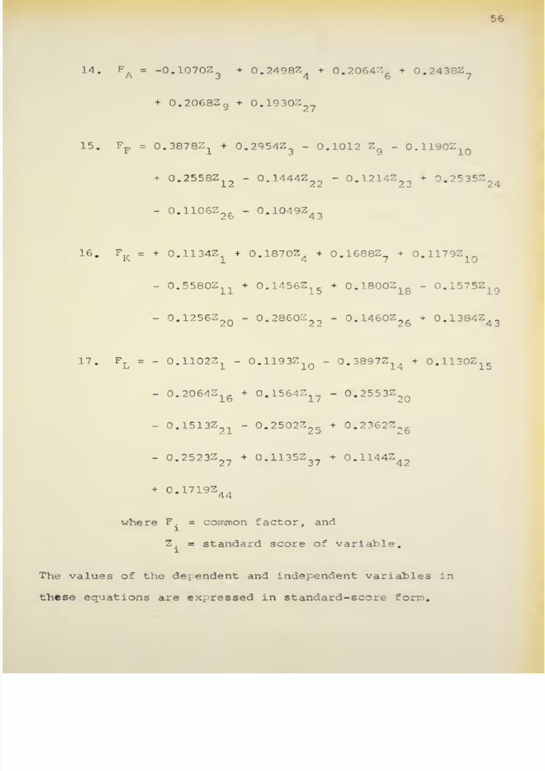
8/11/2019 Speed Delay
http://slidepdf.com/reader/full/speed-delay 70/141
c
.6
14.
F
A
=
-0.1070Z
3
+
0.2498Z
4
+
0.20647^
+
0.2438Z
?
+
0.2063Z
9
+
0.1930Z
27
15.
F
p
=
0.3878Z
1
+
0.2954Z
3
-
0.1012
Z
g
-
0.1190Z
1Q
+
0.2558Z -
0.1444Z..
-
0.1214Z +
0.2535Z-.
12
22
23 24
-
0.1106Z
96
-
0.1049Z
43
16.
F
=
+
0..U34Z,
+
0.1870Z„ +
0.1688Z_
+ 0.1179Z
lo
^
1
4 7
1Q
-
0.5580Z + 0.1456Z
15
+
0.1800Z
lg
-
0.1575Z
lg
-
0.1256Z
20
-
0.28602
-
0.1460Z
26
+
0.1384Z
43
17.
F
L
=
-
0.11023
1
-
0.1193Z
-
0.3897Z
14
+
0.1130Z
15
-
0.2064Z
+
0.1564Z
1?
-
0.2553Z
7Q
-
0.1513Z
- 0.2502Z^
5
+
0.2362Z^
&
-
0.2523Z
2?
+ 0.1135Z
37
+
0.1144Z
42
+
0.1719Z.
44
where
F.
=
common factor,
and
Z.
standard
score
of variable.
The
values
of
the
dependent and independent variables
in
these equations
are expressed
in
standard-score form.

8/11/2019 Speed Delay
http://slidepdf.com/reader/full/speed-delay 71/141
57
Standard
scores
are
computed
by the following
relationship*
18.
Z
i
=
(X
±
-
X
i
)
/
s
i
where
Z
=
standard score of
variable,
X
=
observed
value
of
variable,
X
=
grand
mean
of
variable,
and
s.
=
standard
deviation
of
variable.
The
grand means
and
standard
deviations
for
each
variable
are
listed
in
Table
13,
Appendix
B.
Multiple Linear
Regression and Correlation
Analysis
The
second
phase
of the
multivariate
analysis
of
uninterrupted-flow conditions
was
the
development
of
a
multiple
linear
regression equation
to
predict
mean
travel
speed
from the
significant
variables.
The
38
variables
in
the
revised
correlation
matrix were included in
a
buildup
regression
technique.
(32)
The
routine was
first
performed
without
weighting any of the variables.
This procedure
causes the variables
to
be
entered into
the
equation
in
the
order
of their importance.
The
most
significant variables
were
total
volume,
commercial
establishments, and inter-
secting
streets,
which
were
all
closely related to
the
four
significant factors.
With
these
variables held
in
the
equation by the weighting option of the computer crogram,
different combinations
of
the
remaining variables
were
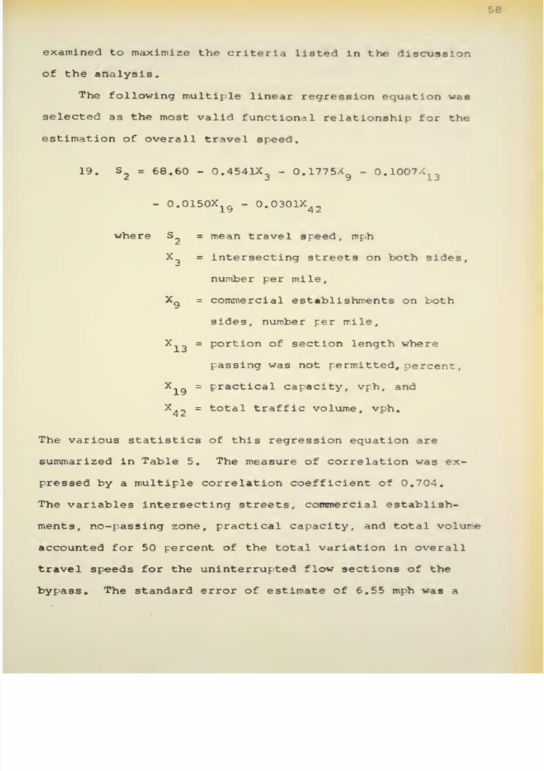
8/11/2019 Speed Delay
http://slidepdf.com/reader/full/speed-delay 72/141
se
examined
to
maximize
the
criteria
listed
in
the
discussion
of the
analysis.
The
following
multiple
linear
regression
equation was
selected
as
the
most valid functional
relationship
for the
estimation of
overall
travel
speed.
19.
S
2
=
68.60
-
0.4541X
3
-
0.1775X
g
-
0.1007/^
-
0.0150X
19
-
0.0301X
42
where
S
=
mean
travel
speed,
mph
X
=
intersecting
streets
on both sides,
number
per mile,
X_
=
commercial establishments
on both
sides, number
per
mile,
X
=
portion
of
section length
where
passing
was
not
permitted,
percent,
X
=
practical
capacity, vph, and
X
=
total
traffic
volume, vph.
The
various statistics
of
this
regression
equation
are
summarized
in
Table
5.
The
measure of
correlation
was
ex-
pressed by
a
multiple correlation
coefficient
of
0.704.
The
variables
intersecting
streets,
commercial establish-
ments, no-passing zone,
practical
capacity,
and
total
volume
accounted
for
50
percent of the total variation in
overall
travel speeds for
the
uninterrupted flow sections of
the
bypass.
The
standard
error
of
estimate
of
6.55
mph was
a
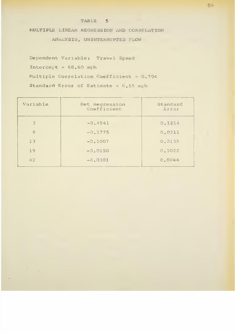
8/11/2019 Speed Delay
http://slidepdf.com/reader/full/speed-delay 73/141
TABLE
5
MULTIPLE LINEAR
REGRESSION
AND
CORRELATION
ANALYSIS,
UNINTERRUPTED FLOW
Dependent
Variable:
Travel Speed
Intercept
=
68.60 mph
Multiple
Correlation Coefficient
=
0.704
Standard
Error
of Estimate
=
6.55
mph
Variable
Net
Regression
Standard
Coefficient Error
3
-0.4541
0.1214
9
-0.177
5
0.0211
13
-0.1007
0.0135
19
-0.0150 0.0022
42
-0.0301
0.0044

8/11/2019 Speed Delay
http://slidepdf.com/reader/full/speed-delay 74/141
60
measure of
the
precision of the
equation.
This
multiple
linear
regression
equation
is
more
reliable
and
appropriate
than the factor
equation for predicting
mean travel
sreeds
on
the
bypass,
as
values
for the
variables
are
easier
to
obtain.
A
significant
portion of the
unexplained variation in
overall travel
speeds was
probably caused by
individual
driver
behavior. Variations were
evident
in
the
driving
habits of
vehicle
operators
as
the test-car
driver
attempted
to
relate
his
speed
to
the average speed
of the
traffic
stream.
In
addition, variations occurred within
the
test
driver
in his
reactions
to
the many
conditions
influencing
his
speed.
Interrupted Flow
The
analysis of interrupted flow
followed
the
same
pattern
as
the investigation
of uninterrupted
flow.
Mean
overall
travel
speeds
and
mean
running speeds were
com-
puted for directional
flows
and for the
combined flow*
in
each section.
These
mean
speeds
are
presented
in
Table
6.
The
overall speed equaled
the
running
speed in
the
north-
west flow of Section
1
because
no stop was required
in
this
direction.
The
mean
speeds in
Sections 17
and
18
were
higher
than for the
other
sections;
these sections
were
longer and the
delays
caused by the signal
were
distributed over
a greater
distance.
Of
the
five
sections
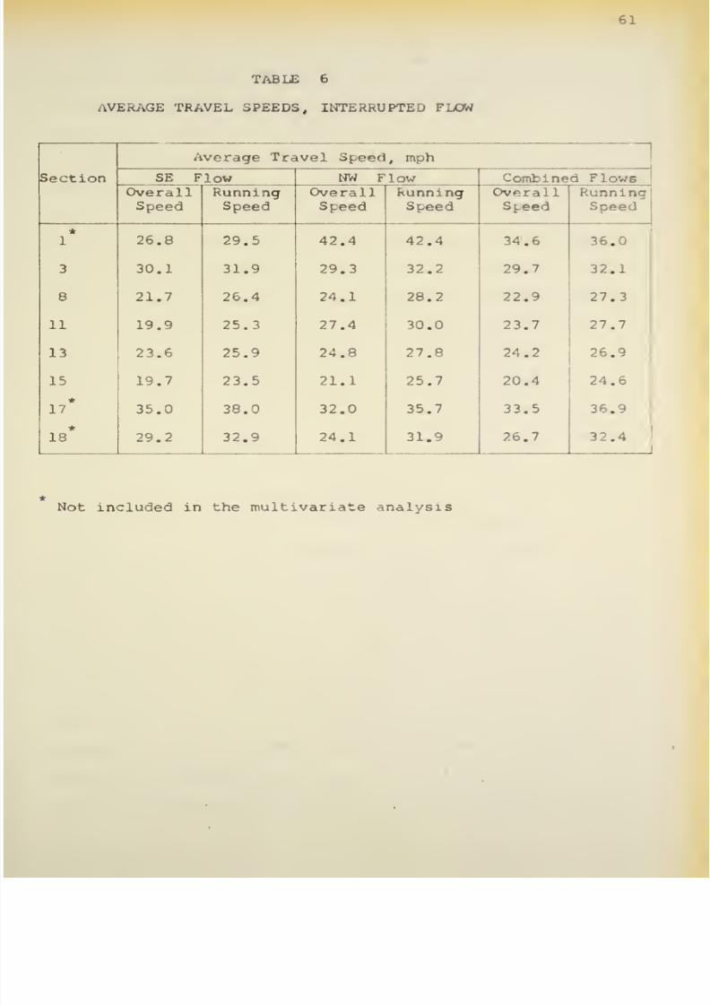
8/11/2019 Speed Delay
http://slidepdf.com/reader/full/speed-delay 75/141
TABLE
6
AVERAGE
TRAVEL
SPEEDS,
INTERRUPTED
FLOW
61
Section
Average Travel
Speed
,
mph
1
SE
Flow
NW
Flow Combined Flows
Overall
Speed
Running
Speed
Overall
Speed
Running
Speed
Overall
Speed
Runnl
Speed
*
1
26.8
29.5 42.4 42.4
34.6 36.0
3
30.1 31.9 29.3 32.2
29.7
32.1
8
21.7 26.4
24.1
28.2
22.9 27.3
11
19.9
25.3 27.4 30.0 23.7
27.7
13
23.6
25.9 24.8 27.8
24.2 26.9
15 19.7 23.5
21.1
25.7
20.4 24.6
17
35.0
38.0 32.0
35.7
33.5
36.9
*
18 29.2
32.9 24.1 31.9
26.7 32.4
Not
included in
the multivariate
analysis

8/11/2019 Speed Delay
http://slidepdf.com/reader/full/speed-delay 76/141
62
included in the
multivariate
analysis,
Section
1,
which
had
a
semi-actuated
traffic
signal (for the
traffic
on
the
road
crossing
the
bypass), had
the
highest
overall travel
speeds.
The
stopped
times for each
section
were
summarized
by
computing
the mean
stopped
time of
each run, the
mean
dura-
tion
of
the
stop,
and
the
percent
of
the
runs
when
stops
occurred.
These
results
are
presented
in
Table
7.
Because
a
stop
sign existed
in the southeast flow
of
Section
1,
the
test vehicle
was always forced
to stop.
The
stopped
times
were
less
at
Section
3
with
the semi-actuated signal
than
at
any
other
signal.
In
Section
11
the
test vehicle
encountered
fewer stopped
times in the
northwest
flow,
as
there
was
a
10-sec
advance
cycle
for
left
turns and
through
movements
in that
direction.
The
test
vehicle
stopped more
times
heading Northwest
than
Southeast
in
Sections
17
and
18.
Vehicles
arrived in
a
random
fashion in
the northwest
flow,
but
traffic
in
the southeast direction was
grouped
in
platoons
formed
at
the
preceding signals.
The
signals
in
these two sections
were
not
interconnected.
The
average delays per vehicle for
both
bypass
approaches
to each intersection included
in the
multivariate
analysis
were computed by the two
methods
described
in the discussion
of
the
procedure.
These
total delays,
including
both
stopped
and running
delays,
are summarized
in
Table
8.
The
delays
computed
by the
two
methods
were
quite
similar.
A
hypo-
thesis test
was performed
to
determine
whether
the
mean
of
the
differences
of
the
computed
and the theoretical
mean

8/11/2019 Speed Delay
http://slidepdf.com/reader/full/speed-delay 77/141
63
TABLE
7
AVERAGE
STOPPED
TIMES,
INTERRUPTED
FLOW
Section
SE
Flow NW
Flow
Average
Stopped
Time
per
Run,
sec
Average
Length
of
Stop,
sec
Percent
of
Runs
When
Stops
Occurred
average
Stopped
Time
per
Run,
sec
Average
Length
of
Stop,
sec
Percent
of
Runs
When
Stops
Occurred
*
1
5.3
5.3
100.0
3 3.7 12.4 30.0 4.1 15.3 27.5
8
10.0
16.6
60.0 8.1 15.0
52.5
11 12.1
18.7 65.0 4.2
10.5 4C.
13 4.8 11.4
42.5
5.7
12.8
45.0
15 9.2 17.5
52.5
8.6 16.5
.0
*
17
5.3
16.4
32.5
8.0 16.3
60.0
*
18 8.8
17.6
50.0
15.8
. ..
... .
. 1
19.6
72.5
Not
included
in
the
multivariate
analysis.
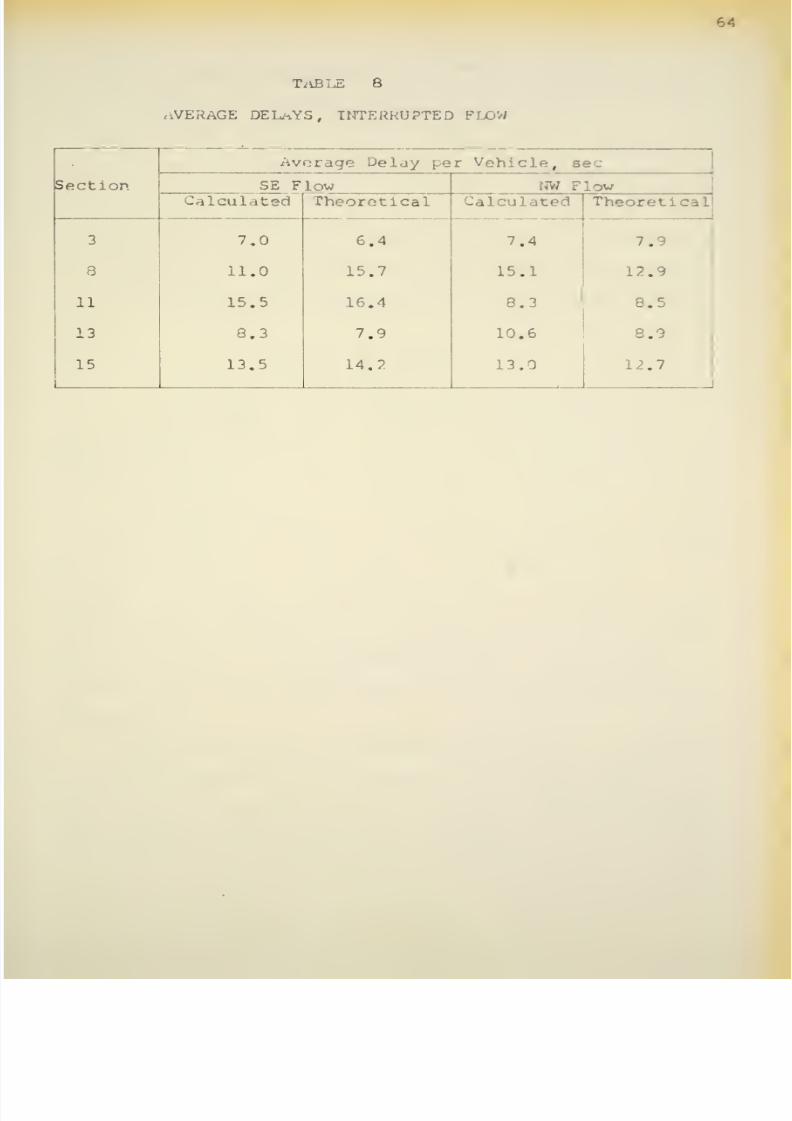
8/11/2019 Speed Delay
http://slidepdf.com/reader/full/speed-delay 78/141
64
TaBLE
8
AVERAGE
DELAYS,
INTERRUPTED
F
Section
Average Delay
pe
r
Vehicle,
sec
SE
Flow
NW
Flow
Calculated
Theoretical Calculated Theoretical
3
7.0
6.4 7.4 7.9
8
11.0
15.7
15.1
12.9
11
15.5 16.4
8.3 8.5
13
8.3
7.9
10.6
8.9
15
1
13.5
14.2 13.0
12.7
i

8/11/2019 Speed Delay
http://slidepdf.com/reader/full/speed-delay 79/141
delays
at each
approach
was
equal
to
zero.
The
hyr-othesis
was
accepted
for
a 5-percent
level
of
significance.
Therefore,
the
results
of
the two computational
methods
did
not
differ
significantly.
Delays were then
computed
from
the
travel-time
data
for
each test-car
run.
The
greatest
delays
occurred at
Sections
8 and 15
for
both flows,
and
Section
11
for
the
southeast
flow.
The
relative
delays
for
each
section corresponded
closely
to
the
stopped
times.
Factor
Analysis
The
correlation
matrix
including variables
46
to 93
inclusive
was
computed
and examined.
The
correlations
of
travel speed
and
delay with the other variables are
listed
in
Table
17,
Appendix
B.
Variables
53,
57,
59,
69,
and
70
and the dependent
variables 92 and 93
were
deleted,
and
the
resultant
matrix
was factorized by the principal-axes
method.
The
factor
analysis
reduced the
41 variables
to 11
factors
which
accounted for 90 percent
of the total
variance
of
the
variables.
The eigenvalue and
that
portion
of the
variation
explained by
each
factor
are
listed
in
Table
18,
Appendix
B.
An
examination
of the rotated-f
actor
matrix,
presented
in
Table
9,
permitted
the
identification
of each factor.
The
following
factors
and their
important
component variables
and respective
coefficients
were
identified*
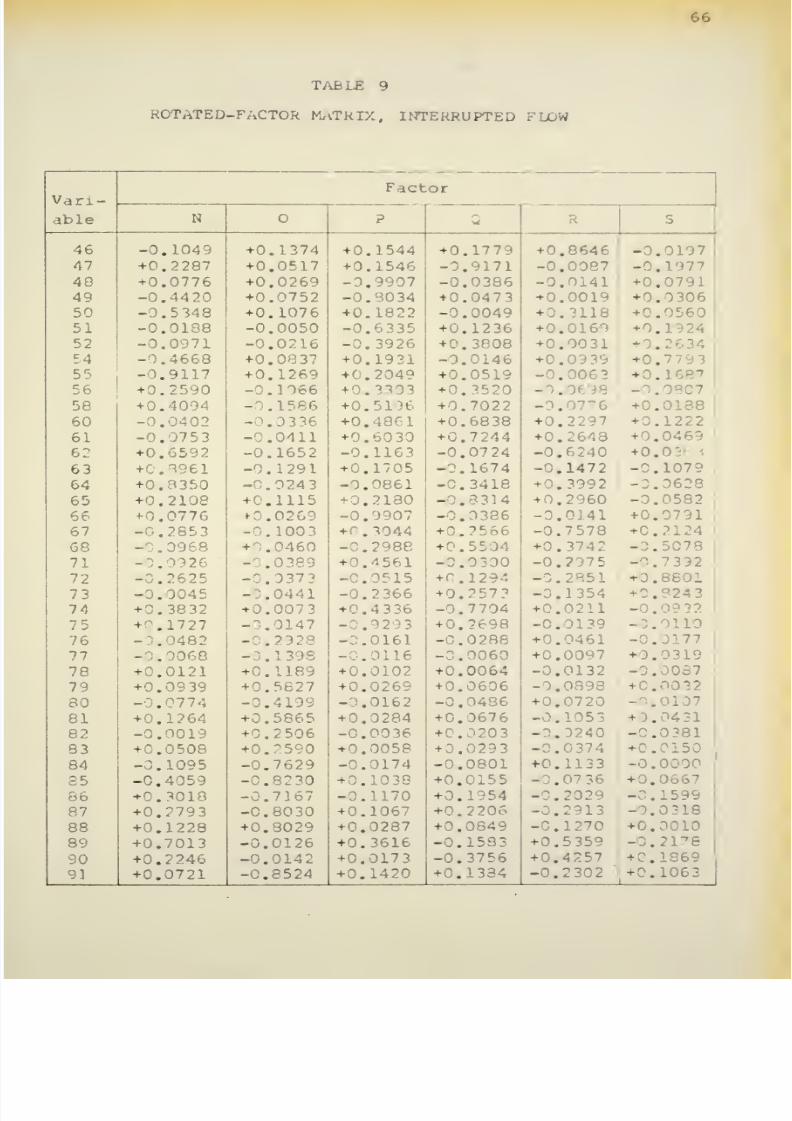
8/11/2019 Speed Delay
http://slidepdf.com/reader/full/speed-delay 80/141
TAb
LE
9
ROTATED-FACTOR
MATRIX,
INTERRUPTED
.
66
Factor
Vari-
able
N
?
Q
R
S
46
-0.1049
+0.1374
+0.1544
+0.1779
+0.8646
-
.0197
47
+0.2287
+0.0517 +0.1546
-0.9171
-o.ooe7
48
+0.0776
+0.0269
-0.9907
-0.0386
-0.0141
+0.0791
49
-0.4420 +0.0752 -0.3034 +0.0473
+0.0019 +0.0306
;
50
-0.5
348
+0.1076
+0.1822
-0.0049
-
.
Lie
-
.
51
-0.0188
-0.0050 -0.6335
+0.1236
+0.0160
+0.1924
52
-0.0971
-0.0216
-
.3926
+0.3808
+0.0031
+
.2634
54
-0.4668
+0.0837
+0.1931 -0.0146
+o.o:-
+0.7793
55
-0.9117
+0.1269
+0.2049 +0.0519
-0.0063
+
0.
56 +0.2590 -0.1066
+
0.
3^0?
+0.3520
-
.
-
.
58
+0.4094
-
.1386 +0.51 +0.7022
-
.07~
+0.0188
60
-0.0402
-
.3336
+0.
+0.6838
+0.2297
-
.1222
61 -0.0753
-
.0411
+0.6030
+0.7244
+0.2648
-
.0469
62
+0.6592
-0.1652
-0.1163 -0.0724
-0.6240
+
0.V
63
»
.8961
-0.1291
+0.1705
-0.1674
-0.1472
-
.1079
64
+0.3350
-^.0243
-3.0861
.3418
-
.3992
.0628
65
+0.2108
+0.1115 .2180
-
.3314
+0.2960
-
.0582
66
+0.0776 +0.0269 -0.0907
-
.0386 .0141
+0.0701
67
-
.2853
-
.
1 00 3
+
.3044
+0.2566
-0.7578
.
68
-
.0968
+
.0460
-
.298e +0.5504
+0.-
;
742
-
.5078
71 -0.0926
-
.0389
+0.4561
-0.3
330
-0
.
2975
— . 332
72
-
.2625
-
.037
3
15
+0.12
-0.2851
-
.8601
73
-0.0045
-
.0441
-0.2366
+0.2573
-
.1354
243
74
+
~.3832
+0.0073
+i
.4336
-0.7704
-
.0211
-0.0932
75
+
.1727
-
.3147 -0.92
+0.2698
-0.31??
-3.
'113
76 .0482
-
,2928
-
.0161
-C.0288
+0.0461
-0.0177
77
-
.0068
-
.1333
.
3: 16
-
.0060
+C.0097
+3.0319
78
+0.0121
+0.1189 +0.0102
+0.0064
-
.3132
-
.
337
79
+0.09
39
+0.5827 +0.0269
1-0.0606
-
.0898
+0.0032
80
-
.
774
-0.4199
-
.0162
-0.0436
-
.0720
-
.
81
+0.1264
+0.5865
-
.3284
+0.0676
-
.
431
82
-0.0019 +0.2506
-0.0036
. 203
-
.
40
-
.
]
31
83
+0.0508
+0.2590
+0.0058
-
. 1
-
.0374
+0.0150
84
-
.1095
-0.7629
-0.3174 -0.0801
+0.1133
30
35
-0.4059
-0.82
30
+0.1038
+0.0155
-
.
-
.
86
+0.3018
-0.7167
-
.1170
+0.1954
-
.2029
-
.1599
87 +0.2793
-C.8030
+0.1067
+0.2206
-0.2913
-
.
18
88
+0.1228
+0.8029
+0.0287
+0.0849 -0.]
+0.0010
89
+0.7013
-0.0126
+0.3616
-0.1583
+0.5359
-0.217
90
+0.2246 -0.0142 +0.0173 -0.3756
+c.
-
.1869
9] +0.0721
-0.8524
+0.1420
+0.1334
-0.2
302
-
.1063

8/11/2019 Speed Delay
http://slidepdf.com/reader/full/speed-delay 81/141
TABLE
9
(continued)
ROTATE
D-F
ACTOR
MATRIX,
INTERRUPTED
FLOW
67
F
actor
Vari
-
able
T
U
V
//
46
-0.0020
+0.0188
+0.0026
+0.0192 +0.0045
47
+0.0012 -0.1810
+0.0024
-0.0007
+0.0062
48 +0.0007
-0.0274
-0.0126
-0.00
39
-
.
1
5 3
49
-0.0043
+0.0433
+0.04
38 +0.0236
+0.0446
50 +0.0124
+0.7288
-0.0293
-0.0011 -0.0
304
51
+0.0055
+0.6973
-0.0024
-0.0044
-0.0017
52
-0.0012 +0.7365 +0.0179 +0.0109 +0.0145
54
-J. 0008
-0.2291
-0.0202
-0.0016
-
.0095
55 -0.0032
-0.0173
+0.0061
+0.0198
+0.0162
56
-
.0004
4
.8096
+0.0233
+0.00
>0
58
-
.0058
+0.1568
+0.0222
+0.0031
-
.
U0O
60 -C.0054
-0.4504
+0.0010
-C.0017
+0.0114
61
-C.0014
+0.1578
+0.0068 +0.0051 +0.0046
62
-
.0172
-0.0401
+0.0526 +0.0208
+0.0321
63
-0.0130
-0.0426
+0.04
37
+0.0163
+0.0252
64 +0.0020
-
.0365
-
.0033
-0,
?084 -0.0110
65 +0.0037
-
.1565
-0.04
37
-0.007
3
-
.0411
66
+0.0007
-0.0274 -0.0126
-0.0039 -0.0153
67
-0.0153
-•.0876
+0.0519 +0.0276 +0.0386
68
+0.0079
+ .2465
- .0745
-0.0243
-0.0539
71
-0.0085
-
.3017
+0.0378 +0.0127 +0.0518
72
-0.0015
-0.0001
+0.0237
+0.0014
+0.0212
73
+0.0043 +0.3475
-0.0232 -0.0097
-0.0405
74
-0.0015
-0.196
3
+0.0170
+0.0C19 +0.0187
75
-0.0011 +0.0853 -0.0108
-0.0012 -0.0194
76
+
.1308
+^.0095 -0.2212
+^.8456
+0.2427
77
+0.1422
+
.
0007
+0.0663
-
.0586
-0.9225
78
.8219
-0.0000 +0.0383 -C.2491
+0.1768
79
+C.5977 -0.0121
+0.2
300
-
.0953
+0.2653
80
+0.1752
+0.0024
-0.1744
-0.6064 +0.3217
81
+0.4812
-0.0166
-0.3519
-0.1240
+0.2051
82
+0.1770
+0.0324
+0.8699
-C.0994
-0.1175
83
-0.7767 -0.0176
-0.1566 +0.1674
+0.0772
84
+0.2603
-C.0060
-0.4207
+0.0107
-0.0656
85
+0.0774 -0.0768
+0.1496
+0.0128
+0.0853
86
+0.0819
+0.1725
-0.1149 -0.0504
-j.1299
87
+0.1025
+0.0779
-0.0806
-0.0137
-0.0281
88
+0.0301
+0.0098
+0.4160
-0.0777
+0.1251
89
-0.0007
-0.0171 +0.0082
+0.0020
+0.0019
90
-0.0533 -0.2679 +0.3943
+0.0524 +0.2180
91
+0.0805
-0.07
47
+0.1577
+0.0140
+0.1030
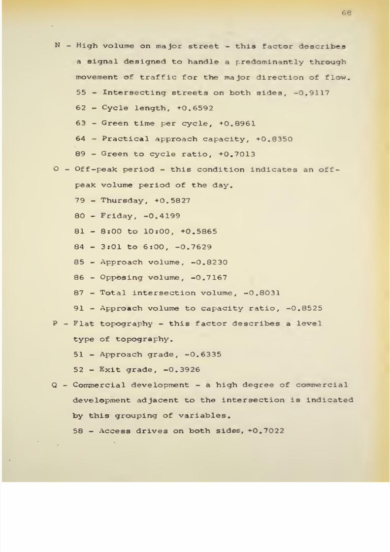
8/11/2019 Speed Delay
http://slidepdf.com/reader/full/speed-delay 82/141
68
N
-
High
volume
on
major
street
-
this factor
describes
a
signal
designed
to
handle
a predominantly
through
movement of
traffic
for
the
major
direction of
flow.
55
-
Intersecting streets
on
both sides, -0.9117
62
-
Cycle
length,
+0.6592
63
-
Green
time
per cycle,
+0.8961
64
-
Practical
approach
capacity,
+0.8350
89
-
Green
to cycle
ratio, +0.7013
-
Off-peak
period
-
this
condition
indicates
an
off-
peak volume period of the day.
79
-
Thursday,
+0.5827
80
-
Friday,
-0.4199
81
-
8:00
to
10:00,
+0.5865
84
-
3:01
to
6:00,
-0.7629
85
-
Approach
volume,
-0.8230
86
-
Opposing
volume,
-0.7167
87
-
Total
intersection volume,
-0.8031
91
-
Approach
volume to capacity ratio,
-0.8525
P
-
Flat topography
-
this
factor describes
a
level
type
of
topography.
51
-
Approach
grade,
-0.6335
52
-
Exit
grade,
-0.3926
Q
-
Commercial
development
-
a
high
degree of commercial
development
adjacent to
the
intersection is indicated
by this
grouping of
variables.
58
-
Access drives
on
both
sides,
+0.7022

8/11/2019 Speed Delay
http://slidepdf.com/reader/full/speed-delay 83/141
69
61
-
Commercial
establishments
on
both sides,
+0.7244
68
-
Regulatory
signs,
+0.5504
R
-
Low
minor-street
traffic
-
this factor describes
an
intersection
with
a
relatively minor
street
intersecting
the
major
traffic
flow.
46
-
Semi-actuated
signal,
+0.8646
62
-
Cycle
length,
-0.6240
87
-
Total intersection
volume,
-0.2913
90
-
Approach to total volume
ratio,
+0.4257
S
-
Concentrated
turning
movements
-
this
factor
indicates
a
large
percentage
of
turning
movements
from both streams of
the
major
traffic
flow
to
the
right
side of the
direction
of travel
of the test
vehicle.
71
-
Left
turns
from directional
travel,
-0.7392
72
-
Right
turns
from directional
travel,
+0.8801
73
-
Left
turns
from opposing
travel,
+0.8243
T
-
Time variations
-
variations in
the
times
and
days
when
the
data were
recorded
are
reflected
in
this
factor,
which is
not completely
defined.
78
-
Wednesday,
-0.8220
79
-
Thursday, +0.5977
81
-
8t00 to 10:00,
+0.4812
83
-
12:01
to
3:00,
-0.7767

8/11/2019 Speed Delay
http://slidepdf.com/reader/full/speed-delay 84/141
70
U
-
Vertical
resistance
-
this group
describes the
vertical
alignment
affecting the traffic flow.
50
-
Length
of
exit
merge
lane,
+0.7288
51
-
Approach
grade,
+0.6978
52
-
Exit
grade,
+0.7365
V
-
Long-distance
travel
-
through traffic
traversing
the
entire
length of
the
bypass is
reflected
in
this factor.
81
-
8:00
to
10:00,
-0.3519
82
-
10:01
to
12:00,
+0.8699
84
-
3:01
to
6:00,
-0.4207
88
-
Commercial
vehicles,
+0.4160
90
-
Approach to total
volume ratio,
+0.3943
W
-
Day-of-week variations
-
the
variation in days
for
which
travel
times
were
obtained
contribute
to
this
partially defined
factor.
76
-
Monday,
+0.8456
78
-
Wednesday,
-0.2492
80
-
Friday,
-0.6065
X
-
Day-of-week
variations
-
further
variations
within
the week
are
evident
in
this group.
77
-
Tuesday,
-0.9226
79
-
Thursday,
+0.2653
80
-
Friday,
+0.3217
Following the
identification
of
each factor,
the factor-
score matrix
was computed.
This
matrix is
presented
in
Table
10.
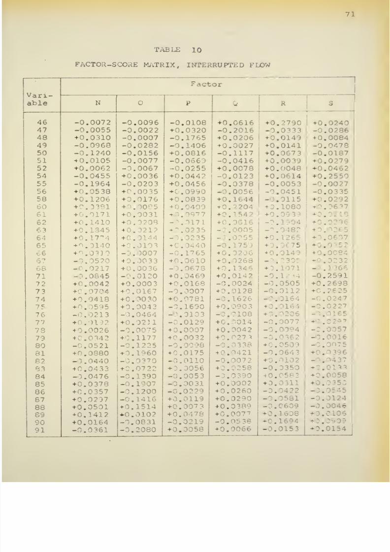
8/11/2019 Speed Delay
http://slidepdf.com/reader/full/speed-delay 85/141
71
TABLE
10
FACTOR-SCORE
MATRIX,
INTERRUPTED
FLOW
Vari-
Factor
able
N
P
-
R
S
46 -0.0072
-0.0096
-0.0108
+0.0616 +0.2790
+0.0240
47 -0.0055
-0.0022
+0.0
320
-0.2016
-
.
^33
-0.0286
48
+0.0310
-0.0007 -0.1765
+0.0206
+0.0149
|
+0.0084
49
-0.0968
-0.0282
-0.1406
+0.0027
+0.0141
-0.0478
50 -0.1240
-0.0156
+0.0816
-0.1117
+0.067
3
'
-0.0187
]
51
+0.0105 -0.0077
-0.0669
-0.0416 +0.0039 +0.0279
52
+0.0062
-).0067 -0.0255
+0.0078
+0.0048
+0.0462
:
54
-0.0455
+0.0036
+0.0441'
-0.0123 +0.0614
+0.2550
55
-0.1964
-
.0203
+0.0456
-0.0378
-0.0053 -0.0027
:
56
+
.0538 +(
.0035
+
.0990
-0.0056
-0.0451 -0.0335
58
+0.1206
+
.0176 +0.08
39
+0.1644
-
.0115 .0292
60
+
).
)381
+
.00
l
?5 +0.0409
+0.2204
*
.1080
-
.
61
+
.0171
.0031
T
. +
.
A?
+0.09
39
-
.
62
+l
. L410
+0.0208
-
. '171
.
16
.
04
-
.
6 3
+
.
J45
+0.021?
-
.0235
-
.
005
.
-
.
64
+0.1774
-
.0144
-
.^2
35
-
.0255
+0.1265
.
65
.
L40
+
.0]
-
.
)440
-
.
.
^5
-
.
66
4
.0310
-
.
007
-
.1765 +0.02
-
.0149
.
B4
-
.
+0.00
3
3
+0.0610
+0.0268
-
.
-
.
68
-
.0217 +0
.
00
.0673
i
.1346
.
)71
-
.
:
>66
71
.0845
-
.0120
+0.0469
+0.01
'
-0.
.
-0.25
72
.0042
+0.000
3
+0.0168
-0.0024
-^.0505
+0.2698
73
+0.07
+
3.
5
167
-0.0007
-
.2128
-0.0112
-
.2625
74
-
.
)418
+0.0030
-
,
^731
-
.1626
-
.0164
-
.0247
75
+0.
595
+0.0043
.1600
+0.0903
*
.
-
-
.0213
-
.0464
-
>.0103
-
.
^108
f
0.0206
.
77
*
.
11
4
.3231
-
.0129
*
-
.
)77 .
78
H
).
^026
-
.
007
5
+0.0007
+0.0042
-
]
, 394
-0.0057
79
*
.0342
+0.1177
4
.0032
73
-
.0016
80
-
.0521
-
.1225
-0.0098
-
.
'38
-
.0509
-
.
61
+
.
0880
-
.1960
*
.0175
-
.
21
-
.
4
3
-
.
96
82
-
)
.
0440
-
.03^0
-
:.0110
-
.
*
.
-02
83
+0.04
33
+
.0722
-
.
J56 .
58
-0.0350 +0.0133
84
-
.0476
-
.1390
-
.0053
-
.0
390
+0.
582
-
.0058
85
+0.0378
-0.1907
-(
.00
31
+0.0002
-
.
11
•
+
0.
86
+C.0357
-0.1200
-
.
'29
-
.0260
-:.
422
-
.
87
+0.0297
-
.1416
+0.0119
+0.0290
-
.0581
-o.oi:
88
+0.0501
+0.1514
-
.0073
+0.0389
-
.
09
-.0046
89
+0.1412
+
.0102
+0.0478
*
.007
-
.1608
-
.0106
90
+0.0164 -0.0831 -0.0219
- .
-
.1694
+0.C
91
-0.0
361
-0.2080
+
.0058
+0.0066 -0.0153
-
.0154

8/11/2019 Speed Delay
http://slidepdf.com/reader/full/speed-delay 86/141
72
T,kBLE
10
(continued)
FACTOR-SCORE
MATRIX,
INTERRUPTED
FLOW
Vari-
Factor
able
T
U
V
/
46
+0.0085
-0.0326
+0.0225
+0.0131
+0.0165
47
+0.0051
+0.0493
-0.0040
-
.
.055
-
. 18
48 +0.0014
-0.0747
-
..0026
-
.0008
.
49
+0.0013
-0.0317
+0.0726
+0.0249
-
.
50
+0.0080
+0.3066
+0.0290
-0.
>317
70
51
-0.0018
+0.2274
+0.0244
+0.0029
+0.03U
52
-0.0064
+0.2
289
+0.0
367
+0.0173
.
>433
54
+0.0066
-0.1007
-0.0321
-0.0144
.0274
55
+0.0049
+0.0031
+0.0413
-
.0119
+0.0278
56
-
.0110
+0.3171
+
.
252
+
.0175
+0.0293
58
-0.0124
+0.0117
-0.0145
+
0.
5C
-0.->982
60
-0.0011
.2488
-
.0240
-
>.0051
-
.0185
61
-0.0032
+0.007 3
4
.0033
.
JJ60
.
)21
62
-0.0186
+0.0006
-
.0071
.1256
-
.
14
63
-(
.0129 +
,0129
-
.
147
+0.
)]
>4
-3.004
3
64
+0.0018
.0034
-
.0333
-
.
'77
-
.0215
65
+0.0099
+0.0351
-
.0425 -1.0162
-
.
66
+0.0014
-
.0747
-
.
026
08 -0.0019
67
-0.0145
-
1.0192
+0.0219
+0.0270
+0.3148
68
+0.0040
*
.
133
-0.0183
-0.0165 -0.0165
71
-0.0060.
-
.0561
l
.
.
'
+
.0163
-
.
72
-
1.0022
-1.0282
-
.0074
-}.
30
38
+0.0010
7
3
-
1.0021
+0.0772
-C
.0435
-
.0112
-
. 395
74
+0.0020
+
.0 382
-
\0098
- .0032
-0.
26
75
-
.0028
-
.0026 +0.0053
-
.0036
76
+0.080
3
+0.0151
-.0263
+0.6813
-
.
1
>33
77
+0.0557 -0.0358
-0.0098
-
.0363
-0.7222
78
-0.4C
+0.0118
+0.0183
-
.2254 +0.1297
70
+0.2968
+0.0024 +0.0755
-3.0316
+0.1876
80
+0.0677
+0.0069 -0.0898
-
.5271
+0.2848
81
+0.2496 -0.0208
-
.^433
-
.1063 +0.09
39
82
+0.0704
+0.0321 +0.5573
+0.0009
-0.0452
83
-0.3657
-0.0061 -0.1143
+
.1107
+0.0208
84
+0.1214
-
.0117
-0.1936 -0.0367
-0.
>2
08
85
+0.0183
-
.0222
+0.1744
+
.0087
+0.1124
86 +0.0208
+0.0402
-0.0240
-
.0555
-0.0675
87
+0.0304 +0.0176 +0.0056
-0.0259 +0.0093
88
+0.0195 +0.0133
+0.1769
-
.0108
-
.0672
89
+0.0011
+0.0135
-0.0159 +0.0017
-0.0088
90
-0.024
3
-0.0664
+0.23°7
+0.0643 +0.1943
91
+0.0189
-?.0238
+0.1973 +0.0094 +0.1342

8/11/2019 Speed Delay
http://slidepdf.com/reader/full/speed-delay 87/141
The
factors were correlated
with
both mean
travel
speed
and
mean
delay;
these factor
correlations
are listed
in
Table
11.
The
same three
factors
were signifiant
at the
5-percent
level
in
accounting
for
the
variations
of
both
dependent
variables.
These
factors
were off-peak
period,
flat topography,
and low
minor-streettraf
f
ic.
Multiple
linear
regression
equations were developed to predict
travel speed and
delay
from these
significant
factors.
The
following
relationship
was
derived to
estimate
travel speed
for interrupted
flow:
20.
S
3
=
24.16
+
10.186
(0.2202F
Q
+
0.1404F
p
+
0.2676F
R
)
where
S
=
mean
travel
speed, mph,
F
=
off-peak
period,
F
=
flat
topography, and
F
=
low minor-street traffic.
The
degree
of
correlation
of this
equation
was
expressed
by
a
multiple
correlation
coefficient
of
0.364.
Approxi-
mately 13 percent
of
the
total
variation in
travel
speed
was
reflected in the
three
significant
factors.
The
standard
error of estimate was 9.49
mph.
Delay
was related
to
the
significant
factors by the
following
formula:
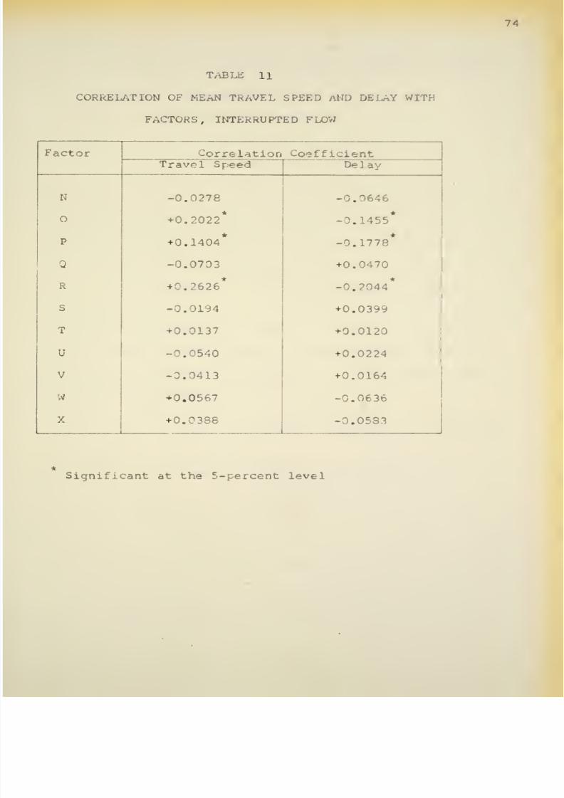
8/11/2019 Speed Delay
http://slidepdf.com/reader/full/speed-delay 88/141
74
TABLE
11
CORRELATION OF MEAN
TRAVEL SPEED
AND
DELAY
WITH
FACTORS,
INTERRUPTED
FLO//
Factor
Correlation
Coefficient
Travel
Speed
Delay
N
-0.0278
-0.0646
O
+0.2022*
-0.1455*
p
+0.1404*
-0.1778*
Q
-0.0703
+0.0470
R
+0.2626*
-0.2044*
S
-0.0194
+0.0399
T
+0.0137
+0.0120
U
-0.0540
+0.0224
V
-0.0413
+0.0164
w
+0.0567 -0.0636
X
+0.0388
-0.05S3
Significant
at the 5-percent level

8/11/2019 Speed Delay
http://slidepdf.com/reader/full/speed-delay 89/141
75
21.
D
1
=
16.49
+
14.23
(-0.1455F
Q
-0.1778F
p
-0.2044P
R
)
where
D
=
mean delay, sec,
F =
off-peak
period,
Fp
=
flat
topography,
and
F
=
low
minor-street
traffic.
The
multiple
correlation
coefficient
of
0.307
measured the
degree of
linear
association
between delay
and the three
significant
factors. The
three
factors
explained only
9
percent of
the total
variation in
delays.
An
index of
precision was
provided
by the
standard error of
estimate
of
13.54
sec.
The
significant
factors
were
evaluated
in
terms of
the
original
study variables.
The
following
multiple
linear
regression
equations
were
developed in
standard-score
form
to
express
these factors:
22.
F
Q
=
0.1177Z
7g
-
0.1225Z
Q0
+
0.1960Z
81
- 0.1390Zq
4
-
0.1907Z
85
-
0.1200Z
86
-
0.1416Z
8?
+
0.1514Z
88
-
0.2080Z
gi
23.
F
p
=
-0.1765Z
48
-
0.1406Z
4g
- 0.1765Z
66
-
0.1690Z
75
24.
F
R
=
0.2790Z
46
+
0.1080Z
60
-0.1904Z
62
+
0.1265Z
64

8/11/2019 Speed Delay
http://slidepdf.com/reader/full/speed-delay 90/141
76
-
0.2305Z
67
+ 0.1071Z
6Q
-
0.1234Z
71
+
0.1608Zg
g
+
0.1694Z
9Q
where
F
=
common
factor and
Z
=
standard
score
of
variable.
The
standard
scores
of
each
variable
are
computed
from
Equa-
tion
18.
The
means and
standard deviations of
each
variable
are
listed
in
Table
16,
Appendix
B
#
Multiple
Linear
Regression
and Correlation Analysis
Multiple
linear
regression equations were developed
to
estimate
travel speeds
and
delays
for
interrupted flow
as
functions
of
the
significant variables.
The
techniques
for
deriving
these relationships were similar
to
the
standards followed
in
the
uninterrupted
flow
analysis.
The
multiple linear
equations
expressing
overall
travel
speed and
delay
as
functions
of the
significant
variables
are
presented in
Table
12.
The
speed
relation-
ship has
the
following form:
25.
S
4
=
?8.595
-
0.4165X
51
-
0.2118X
62
-
0.0120Xg
5
-
0.0170X
Q7
+
29.4800X
Q9
where
S
=
mean
travel
speed, mph.

8/11/2019 Speed Delay
http://slidepdf.com/reader/full/speed-delay 91/141
77
TABLE
12
MULTIPLE
LINEAR REGRESSION AND
CORRELATION
ANALYSIS, INTERRUPTED FLOW
Dependent Variable
:
Travel
Speed
Intercept
=
28.59 mph
Multiple
Correlation
Coefficient
=
0.36E
Standard
Error
of
Estimate
=
9.53
mph
'
Variable
Net
Regression
Coefficient
Standard
Error
51
-0.4165 0.3235
62
-^.2118 0.0587
85
-0.0120 0.0280
87
-0.0170
0.0104
89
+29.4800
7.4739

8/11/2019 Speed Delay
http://slidepdf.com/reader/full/speed-delay 92/141
78
tab IE
12
(continued)
MULTIPLE LINEAR
kEGkESSION
aND
CGRRELATIGN
ANALYSIS,
INTERRUPTED
FLOW
Dependent
Variable:
Travel Delay
Intercept
=
11.95
sec
Multiple
Correlation Coefficient.
=
0.326
Standard Error of
Estimate
-
13.544
mph
Variable
Net Regression
Standard
Coefficient
Error
49
+0.0052
0.0024
62
+0.2299
0.0833
85
+0.0135
0.0401
87
+0.0168
0.0154
89
-35.7935
12.7107

8/11/2019 Speed Delay
http://slidepdf.com/reader/full/speed-delay 93/141
70
X
=
average algebraic
grade
of
approach,
percent,
X
=
cycle
length
cf
traffic
signal, sec,
X
=
traffic
volume
approaching
the
intersection
in
the
direction of
travel, vehicles
per
15
min,
X
=
total traffic volume
entering the inter-
section
on
all
four approaches,
vehicles
per
15
min,
and
X
=
green time
to
cycle
length
ratio.
The
degree
of
linear
correlation
was
indicated by
a
multiple
correlation
coefficient of
0.368.
The
significant
variables
(approach grade, cycle length,
approach
volume, total inter-
section
volume, and
green-to-cycle
ratio)
accounted
for
14
percent of the variation in travel speeds.
The
reliability
of
the
estimate
was
expressed
by
a
standard error of 9.53
mph.
The
following
multiple
linear
regression equation
for
travel delay
was
evolved:
26.
D
2
=
11.951
+
0.0052X
4g
+ 0.2299X
62
+
0.0135X
g5
+ 0.0168X
87
-
35.7935X
gg
8/11/2019 Speed Delay
http://slidepdf.com/reader/full/speed-delay 94/141
80
where
D
=
mean
travel
delay, sec,
X
=
length
of
approach
to
special
turning
lane,
ft,
X
62
=
cvcle
length
of traffic
signal,
sec,
X
_=
traffic
volume
approaching the
intersection
in
the direction
of
travel, vehicles
per
15
min,
X
=
total traffic
volume entering
the
inter-
section
on
all
four
approaches,
vehicles
per 15
min,
and
X
=
green
time to
cycle
length ratio.
By
The
correlation
coefficient
of
0.326 measured
the
degree
of
the
functional
relationship
of
the variables.
Approxi-
mately
11 percent
of the
variability
in
delay was
explained
by
the independent
variables. These five
variables
were
length
of
approach to
turning
lane,
cycle
length,
approach
volume, total intersection
volume,
and green-to-cycle
ratio.
The
standard
error of estimate was
13.54
mph. The
sign
of the
regression
coefficient
of the
length
of
approach
to
turning
lane
variable was
contrary
to
expectation.
The
plus
sign
indicated that
delay
increased as the
length
of
the
approach
increased
in combination
with the
other
variables
in the
model.
The
length
of the
approach,
how-
ever,
was
associated
with
a
high
-volume intersection and
with
a
relatively
high
number of
turning movements. These
conditions
contributed
to
the
increased
delays.

8/11/2019 Speed Delay
http://slidepdf.com/reader/full/speed-delay 95/141
81
The
multiple
correlation
coefficients
of
these
two
regression
equations
were
lower
for
the analysis
of
the
interrupted
flow
versus
those
for
the
uninterrupted flow.
Overall travel
speeds
and
delays
at
signalized intersections
depended
greatly
on
whether
or
not
the
vehicle was
required
to
stop. This
condition
of chance
was
not accounted
for
in
the
analysis.
In
addition,
those variables which were
significant
in
the final
models
exhibited
little variation
among the
study
intersections.
The
unexplained
variability
with
individual
drivers
was
again evident
in
the
analysis.
Recommended
Imrrovements
The
results
of the analyses
of
uninterrupted
and
interrupted
flow
were
applied
for
the
recommendation
of
traffic
engineering improvements
to minimize delays
on
the
U.S.
52
Bypass.
The
major
delays to the traffic
stream
occurred
at the
signalized intersections.
These
delays
are
evident
by an
examination
of the average
travel speeds
for
all
sections depicted
in
Figure
5.
The
significant
factors
in
causing
the
delays
were
largely
associated
with
the design
of
the 6ignal
and
the
approach
volumes.
Reduc-
tions
in speed
for the
uninterrupted flow portions of
the
bypass were
mainly
influenced by
the
degree
of
commercial
development,
the
related number
of access points, and by
volume.
The
annual
average
daily
traffic
of each
section
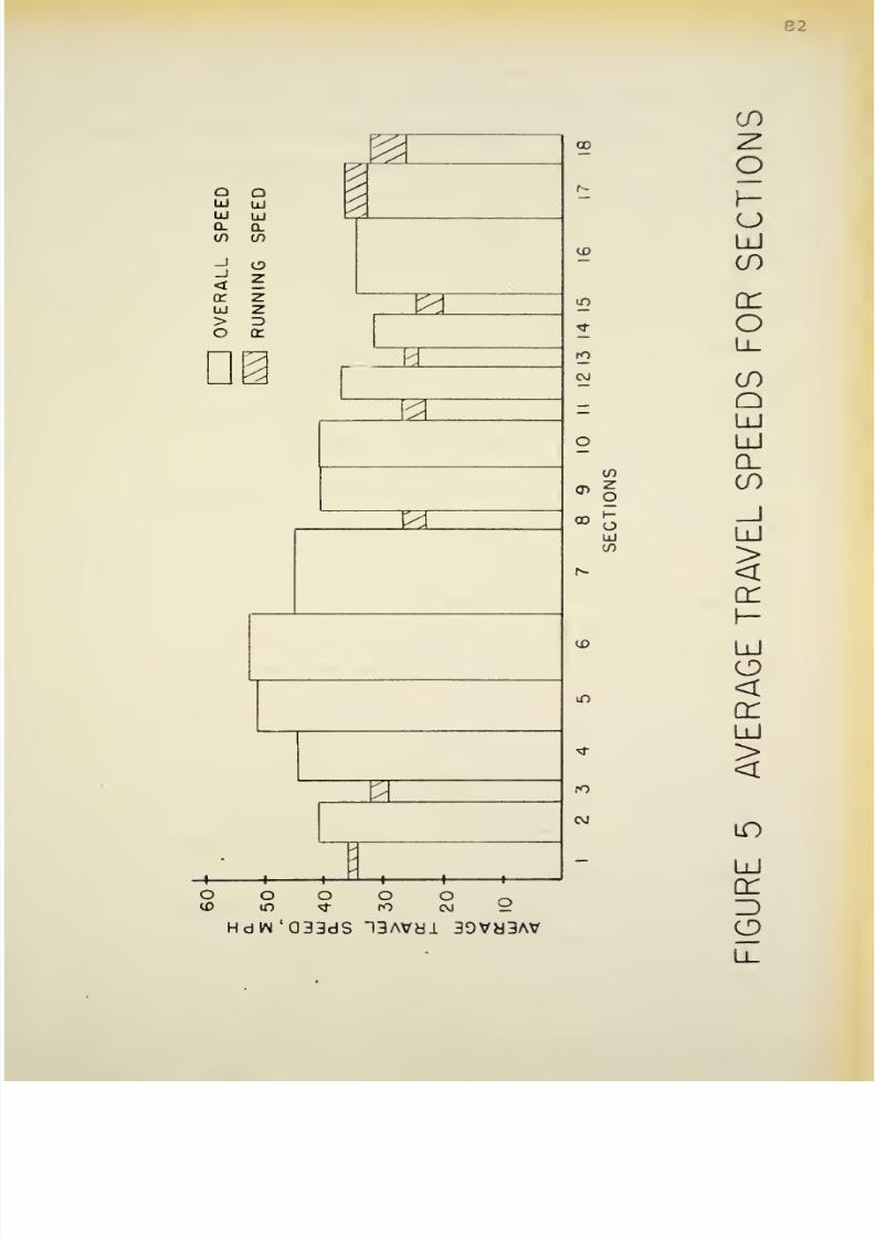
8/11/2019 Speed Delay
http://slidepdf.com/reader/full/speed-delay 96/141
82
UJ
o_
GO
o
UJ
UJ
0.
CO
<
?
cr
z
ui
z
>
3
o
cr
i-'.
o
o
m
o
o
fO
O
CO
CO
in
CJ
go
(T
oo
CO
u
LU
(f)
cr
o
Ll_
CO
o
LU
LU
Q_
(/)
—
(J
UJ
LU
CO
>
N-
<
cr
h-
<x>
LU
ID
in
<
cr
LU
<j-
><
ro
OJ
m
—
LU
cr
HdW'Q33dS
13AVH1
30VH3AV
o

8/11/2019 Speed Delay
http://slidepdf.com/reader/full/speed-delay 97/141
83
is
shown in Figure
6.
The
lack
of
capacity
of
the
two-
lane
highway was
also evident
in
the
peak-hour
}«riods.
In
compliance
with
these
general
conclusions,
the fol-
lowing
recommendations
were
made
to aid
in
reducing
delays.
Certain
modifications
are
first
presented
for
immediate
implementation
at minimum
cost. These
improvements
are
to
serve until
a
long-range
plan
of
complete
reconstruction
is
carried
out.
A
second
group
of
recommendations
apply
to such
reconstruction.
Short-Range
Improvements
The
following
traffic
engineering
techniques are
suggested
for immediate
consideration
to
minimize delays
and
increase
overall
travel
speed on
the U.S.
52
Bypass.
1.
The
design of
the
existing traffic signals
should
be
carefully
reviewed with consideration given to
the
proper assignment
of
green
time
for all inter-
section
approaches.
2.
Turning
lanes
at
the
signalized
intersections
should be
improved
and
clearly marked. Lanes
should
be
designated
for
the proper
traffic
movements.
3.
Entrances
to
commercial
establishments
should
be
limited and
clearly
channelized.
In
many
cases,
drivers
can
presently
leave
the
highway
at
any

8/11/2019 Speed Delay
http://slidepdf.com/reader/full/speed-delay 98/141
94
o
O
o
o
o
CVJ
o
o
o.
o
o
o
o
o
o
o
in
00
OUdVHl
A1IVQ
39VH3AV
IVHNNV
—
Li_
r--
U_
<
cr
10
h-
m
>
<t
_i
m
<
C\J
O
—
LU
o
CO
<
CO
<T>
o
cr
^
CO
o
LU
o
I
s
-
UJ
CO
>
<
o
_J
LU
<
(/)
tO
Z>
^
cr
m
2
o
<
Li_
^
rO
CD
CM
LU
cr
o
Ll
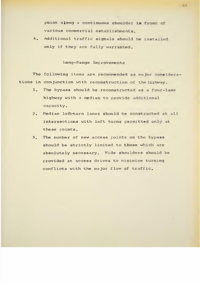
8/11/2019 Speed Delay
http://slidepdf.com/reader/full/speed-delay 99/141
l
c
.
point
along
a
continuous
shoulder
in
front
of
various
commercial
establishments.
4.
Additional
traffic
signals
should
be
installed
only
if
they
are
fully
warranted.
Long-Range
Improvements
The
following
items
are
recommended
as
major
considera-
tions
in
conjunction
with
reconstruction
of the
highway.
1.
The
bypass should
be
reconstructed
as a four-lane
highway
with
a
median to provide
additional
capacity.
2.
Median left-turn
lanes should be
constructed
at
all
intersections
with
left turns permitted only at
these
points.
3.
The
number
of
new access
;x>ints on
the bypass
should
be
strictly
limited to
those
which
are
absolutely
necessary.
Wide
shoulders
should be
provided at
access
drives
to
minimize turning
conflicts
with
the
major
flow of traffic.

8/11/2019 Speed Delay
http://slidepdf.com/reader/full/speed-delay 100/141
B€
SUMMARY
OF
RESULTS
AND
CONCLUSIONS
The
following
conclusions
were
derived
from
the
results
of the multivariate
analyses of overall
travel
speed
and
delay
on
the
U.S.
52
Bypass
located
in
Lafayette, Indiana.
The
movements of
traffic
on
the
bypass
were
classified
by
two categories. Uninterrupted
flow
was
distinguished
from
interrupted flow
at
signalized
intersections
where traffic
was
required
to stop
for
the
red-signal indication.
These
conclusions are
valid only
for
the
flow
of traffic
on
the
bypass,
but
these
findings also
serve as
generalizations
of
the
significant
determinants
of
travel
speeds
and delays
on
similar
type facilities.
1.
The
overall travel
speeds of the
uninterrupted-
flow
portions
of the
bypass
were
influenced
by
four
significant
factors.
Commercial develop-
ment,
urban
development,
and
stream
friction
were
negatively
related
to
speed,
and
the
remaining
factor,
rural
development,
was
associated
with
travel
speed in a
positive
manner.
Commercial
development
accounted for
30 percent
of
the
variation
in
travel
speed.

8/11/2019 Speed Delay
http://slidepdf.com/reader/full/speed-delay 101/141
87
2.
Five
variables
were
significant
in
the
prediction
of
mean
overall
travel
steeds for
the uninterrupted
flow
sections. These
variables,
which
were
total
number
of street
intersections
[«r
mile,
total
number
of
commercial
establishments
per mile,
percent
of
section
where
passing was not per-
mitted,
practical
capacity,
and
total
volume,
were
all negatively
related
with
travel speed.
3.
For
the
interrupted-flow
portions
the
factors
which
significantly
explained
both
overall
travel
speeds
and
delays
were
off-peak
period,
flat
topography,
and
low
minor-street
traffic.
These
three factors
were
associated with
increased travel speeds
and
decreased
delays.
4.
The
variables of cycle
length, traffic
volume
approaching
the
intersection
in the
direction of
travel,
and
total intersection volume
contributed
to
decreased
speeds
and
increased delays.
The
green
time
to cycle
length
ratio accounted
for
significant variations
in
travel speeds
and
delays in
a
positive
and
negative
manner,
respectively,
The approach
grade
of the
intersection
was
nega-
tively
related
to speed, and the
length
of
the
approach
to
the turning
lane was
positively
associated
with
delay.

8/11/2019 Speed Delay
http://slidepdf.com/reader/full/speed-delay 102/141
bft
5.
Multiple
linear regression equations
were
developed
to
estimate
mean
travel
speeds
and
delays
from
the
significant
factors and
variables
for
both
flows.
Approximately
50
percent
of
th: variation
in
speed
of uninterrupted
flow was
explained
and
10 to 15
percent of the
variation in
travel
speeds
and
delays
at
signalized
intersections
was
accounted
for.
The
reliability
of
these
relation-
ships was limited
by
the
unknown
effects
of
driver
behavior
which
was
not included in the
analysis.
In
addition,
delays
at
traffic
signals
were
largely
dependent on
whether
or not
a
stop
occurred.

8/11/2019 Speed Delay
http://slidepdf.com/reader/full/speed-delay 103/141
SUGGESTIONS
FOR
FURTHER
RESEARCH
The
findings
of
this
investigation
have
brought
about
several
possibilities
for
further
research. The
following
items
are
suggested
for
continued
study.
1.
The
multiple
linear
regression
equations
to
predict
mean travel
speeds for
uninterrupted
and interrupted
flows
should
be
verified
on
another two-lane,
urban
highway. These
statistical models
may be valid as
reliable
estimators of
travel speeds
on
similar
types of
highways.
2.
Similar multiple
linear
regression
models
should
be
developed
for multi-lane highways in
urban
areas.
Different
groups
of factors and
variables
with
adjusted
coefficients
and
intercepts may
adequately
describe
the
flow
of traffic
on
multi-
lane
facilities.
3.
The
analysis
of interrupted
flow at signalized
intersections should
be
expanded to
include
a
larger
sample of
intersection
conditions.
A
greater range
in
the
values
of
the
significant
variables
should
produce
a
more
reliable
multiple
linear
regression
equation.

8/11/2019 Speed Delay
http://slidepdf.com/reader/full/speed-delay 104/141
4. Non-linear
forms
of
the
variables and Interaction
terms
may
increase
the
precision
of
the estimates
of travel
speeds and
delays.
The
statistical
models
developed
in
this
study did
not
include
curvilinear
or
Joint
functional
relationships.
5.
After
the
bypass
has
been
reconstructed,
travel-
speed
and delay data should
be
collected
and
analyzed
again
to
determine the
effects of
the
improvements.
Statistical
models developed for
this
facility
could
form
the basis of
travel-speed
predictions
for mult
i
-lane,
urban highways.

8/11/2019 Speed Delay
http://slidepdf.com/reader/full/speed-delay 105/141
BIBLIOGRAPHY

8/11/2019 Speed Delay
http://slidepdf.com/reader/full/speed-delay 106/141
92
REFEn£NCES
1.
Berry,
D. S.,
Evaluation
of
Techniques
for Detenrining
Over-All
Travel
Time,
Proceedings . Highway
Research
Board, Vol.
31,
1952,
pp.
429-440.
2.
Berry,
D.
S.,
and
C.
J.
Van
Til,
A
Comparison
of
Three
Methods
for
Measuring
Delay
at
intersections,
Traffic
Engineering
.
Vol.
25,
December
1954,
pp.
93-99.
3.
Bone,
A.
J.,
Travel
-Time
and
Gasoline-Consumption
Studies
in
Boston,
Proceedings
.
Highway
Research
Board,
Vol.
31,
1952,
pp.
440-466.
4.
Clifford,
E.
J.,
The
Measurement of
Traffic
Flow,
Traffic
Engineering.
Vol.
26,
March,
1956,
pp.
243-246.
5.
Coleman,
R.
R., A
Study
of Urban
Travel Times
in Pennsyl-
vania
Cities,
Bulletin
303
.
Highway Research
Board,
l^^i,
pp.
62-75.
6.
Cribbins,
P.
D., J.
W.
Horn,
and
C.
E.
Vick, Develop-
ment and
Use
of
Maximum-Car
Techniques for
Measuring
Travel
Time, Bulletin
303 . Highway
Research
Board,
1?
,
pp.
94-102.
7.
Determining Travel Time
.
Procedure Manual
3E
,
National
Committee
on
Urban
Transportation,
1958.
8.
Dixon,
W.
J.
,
Biomedical
Computer
Programs
.
Health
Sciences
Computing
Facility, University of California,
Los
Angeles,
January
1,
1964,
pp.
169-184,
233-257.
9.
Hall,
E. M.,
and
G.
Stephen,
Jr.,
Travel
Time-An
Effective Measure of
Congestion
and
Level
of
Service,
Proceedings
.
Highway Research
Board,
Vol.
38,
1959,
pp.
511-529.
10.
Harman,
H. H.
f
Modern
Factor
Analysis
.
Chicago,
The
University
of
Chicago
Press,
1960.
11.
Highway
Capacity
Manual
.
U.
S.
Department
of
Commerce,
Bureau
of
Public
Roads,
Washington,
D.
C., 0.
S.
Govern-
ment
Printing
Office,
1950,
pp.
35-10T.

8/11/2019 Speed Delay
http://slidepdf.com/reader/full/speed-delay 107/141
12.
Hixon,
C.
D.,
An
Analysis
of
Urban Travel
Times
and
Traffic
Volume
Characteristics,
Bulletin
303
. Highway
Research
Board,
1961,
pp.
103-116.
13.
Horn,
J.
W.,
p.
d.
Cribbins, J. D.
Blackburn,
and
C.
E.
Vick,
Jr.,
Effects
of
Commercial
Roadside
D-
Trent
on
Traffic
Flow
in
North
Carolina,
Bulletin
303
.
Highway
Research
Board,
1961,
pp.
76-93.
14.
Johnston,
W.
W.
, Travel
Time
and
Planning, Traffic
Quarterly.
Vol.
10,
January
1950,
pp.
67-78.
15.
Keefer,
L.
E.
#
The
Relation Between
Speed
and Volume
on
Urban
Streets,
Chicago
Area
Transportation
Study,
1958,
unpublished.
16. Matson,
T.
M.,
W.
S.
Smith,
and
F.
W.
Hurd, Traffic
Engineering
,
New
York,
McGraw-Hill
Book
Company,
Inc.,
1955,
pp.
327-334.
17.
Mueller,
E. A.,
Recent
Speed
and
Delay
Instruments,
Traffic
Engineering
.
Vol.
25,
December
1954,
pp.
100-114.
18.
Oppenlander,
J.
C.,
Multivariate
Analysis
of Vehicular
Speeds,
Record
35
f
Highway Research Board,
1963,
pc.
41-77.
19.
Oppenlander,
J.
C.,
W.
F.
Bunte,
and
P.
L. Kadakia,
Sample Size
Requirements
for
Vehicular
Speed Studies,
Bulletin
281
.
Highway
Research
Board,
1961,
pp.
68-86.
20.
Oppenlander,
J.
C.,
and
R. F.
Dawson,
Criteria
for
Balanced Geometric Design of
Two-Lane,
Rural
Highways,
Highway
Research
Board,
in
press.
21.
Ostle,
B.
#
Statistics
in
Research
.
Ames,
Iowa,
The
Iowa
State
University Press,
1963.
22.
Rodgers,
L. M.
,
A
New
Traffic
Delay
Measuring Device,
Traffic Engineering
.
Vol.
27,
February
1957,
pp.
223-228.
23.
Rothrock,
C. A.,
and
L.
E.
Keefer,
Measurement
of
Urban
Traffic
Congestion,
Bulletin 156
.
Highway
Research
Board,
1957,
pp.
1-13.
24.
Sawhill,
R. B.,
and
K. C.
Crandall,
Some
Measurable
Qualities
of
Traffic
Service
Influenced by
Freeways,
Research
Report
No.
11,
Transportation
Research Group,
University
of
Washington,
June
1964.
8/11/2019 Speed Delay
http://slidepdf.com/reader/full/speed-delay 108/141
25.
Stohner,
W.
R.
f
Speeds
of
Passenger
Cars
on
Wet
and
Dry
Pavements,
Bulletin
139
f
Highway Research
Hoard,
1956,
pp.
79-84.
26.
Versace,
J.,
Factor
Analysis of
Roadway and
Accident
Data,
Bulletin
240
,
Highway
Research
Board,
iy
r
,
pp.
24-32.
27.
Volk,
W.
M.,
Effect
of
Type
of
Control on
Intersection
Delay,
Proceedings
.
Highway Research
Board,
1956,
Vol.
35,
pp.
523-533.
28.
Walker,
W.
P.,
Speed
and Travel
Time
Measurement
in
Urban
Areas,
Bulletin 156 .
Highway Research
Board,
1957,
pp.
27-44.
29.
Wortman,
R.
H., A
Multivariate
Analysis of
Vehicular
Speeds
on
Four-Lane
Highways, Civil
Engineering
Studies,
Traffic Engineering
Series
No.
13,
University
of
Illinois,
1963.

8/11/2019 Speed Delay
http://slidepdf.com/reader/full/speed-delay 109/141
95
COMPUTER
PROGRAMS
30.
Correlation Program,
BIMD 2D,
Statistical
laboratory
Library Program,
Purdue University.
31.
Factor Analysis,
BIMD
3M,
Statistical
Laboratory
Library Program,
Purdue
University.
32.
Stepwise
Regression,
BIMD
2R,
Statistical
Laboratory
Library Program,
Purdue
University.

8/11/2019 Speed Delay
http://slidepdf.com/reader/full/speed-delay 110/141

8/11/2019 Speed Delay
http://slidepdf.com/reader/full/speed-delay 111/141
97
APPENDIX
A
TEST
SECTIONS,
U.S.
52
BYPASS
(SCALE
1
=
300'
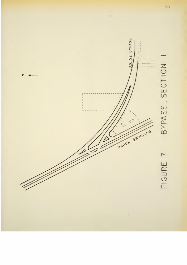
8/11/2019 Speed Delay
http://slidepdf.com/reader/full/speed-delay 112/141
96
(/>
W
<
CL
>-
CD
.
<\l
If)
/
uil
o
o
LlI
CO
CO
CO
<
CL
>
CD
Ld
cr
Z)
CD
Ll_

8/11/2019 Speed Delay
http://slidepdf.com/reader/full/speed-delay 113/141
C\J
D
O
o
LU
IF
CO
CO
<
a.
>-
oo
LU
cr
o
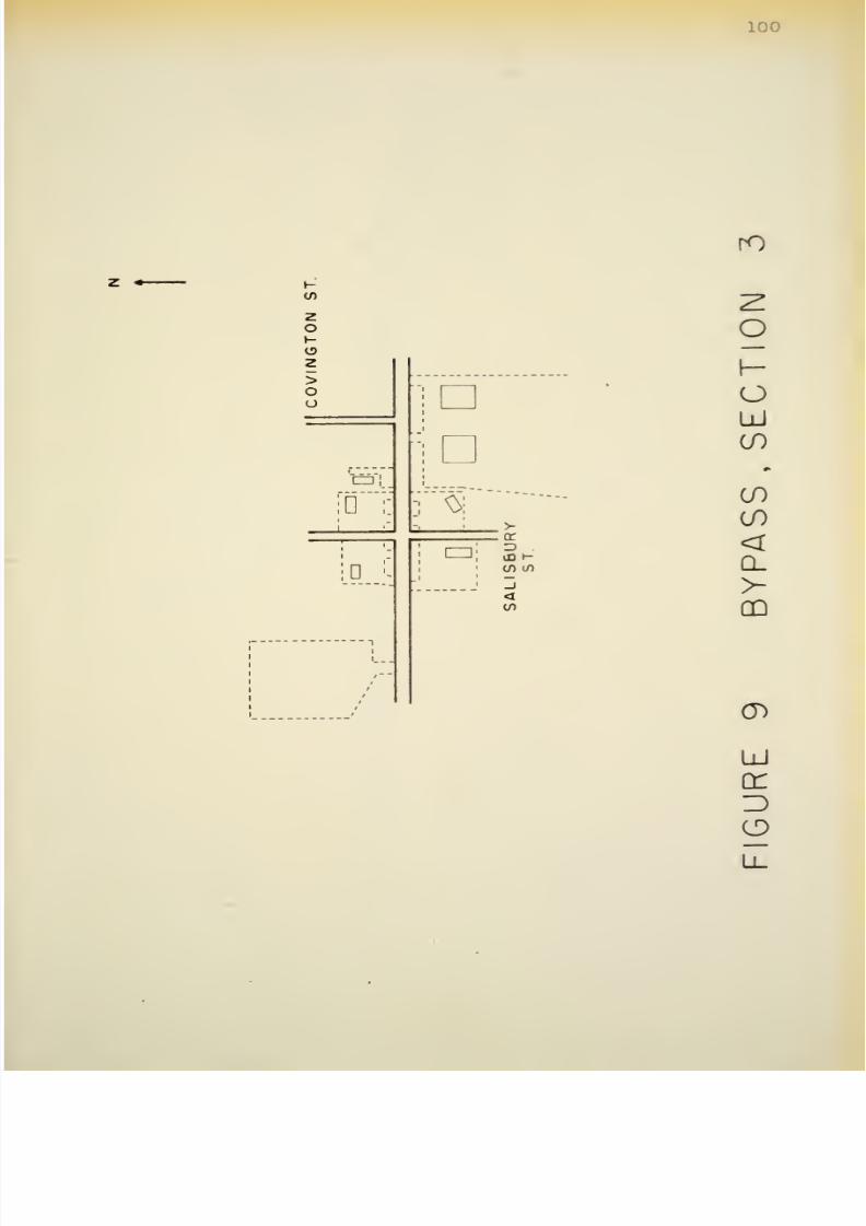
8/11/2019 Speed Delay
http://slidepdf.com/reader/full/speed-delay 114/141
100
z
*-
en
2
O
I-
o
>
o
o
CZD
D
D
Q
,
cr
=) .
<
to
rO
O
O
LU
CO
CO
CO
<
CL
>
GO
LU
DC
Z>
o
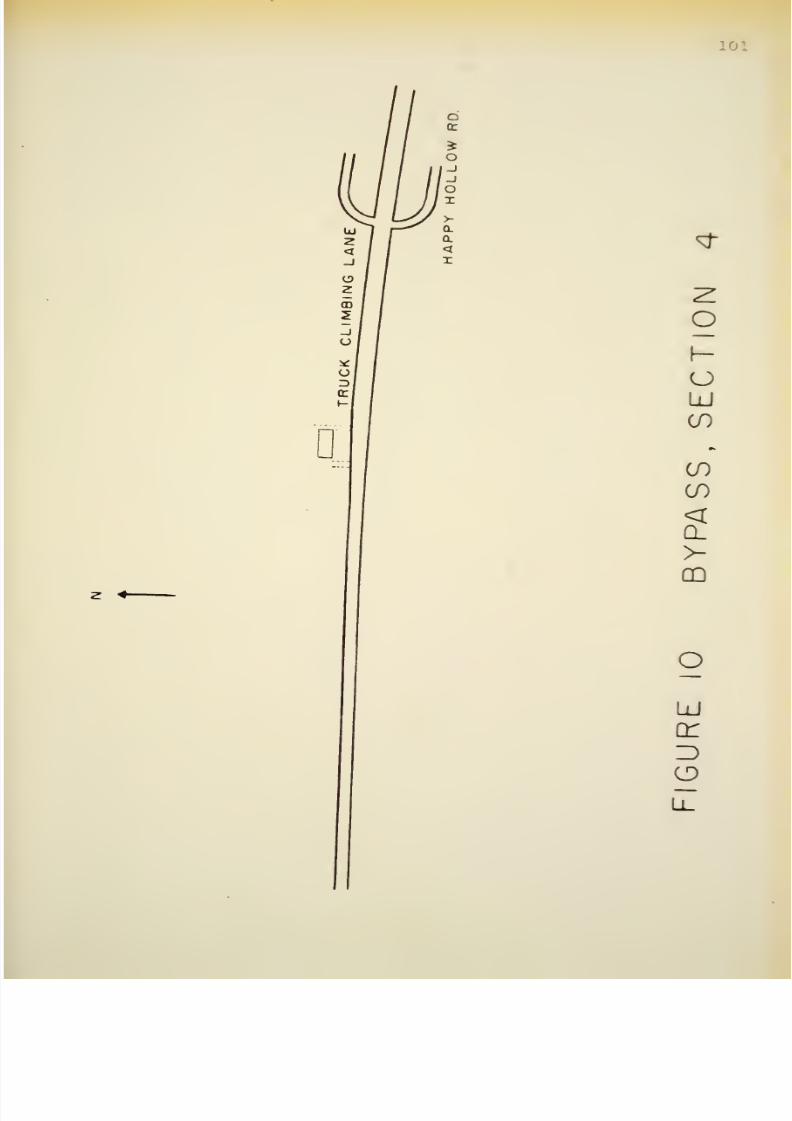
8/11/2019 Speed Delay
http://slidepdf.com/reader/full/speed-delay 115/141
10]
o
O
o
Ld
CO
pi
LD
CO
<
CL
>-
O
LU
or
z>
o

8/11/2019 Speed Delay
http://slidepdf.com/reader/full/speed-delay 116/141
u
lO
o
o
LU
CO
UJ
z
4-
Ci>
CD
CO
CO
<
CL
>
LU
U_

8/11/2019 Speed Delay
http://slidepdf.com/reader/full/speed-delay 117/141
2
+
<
CD
O
O
LU
00
CO
<
Q_
CO
Ld
(T
ID
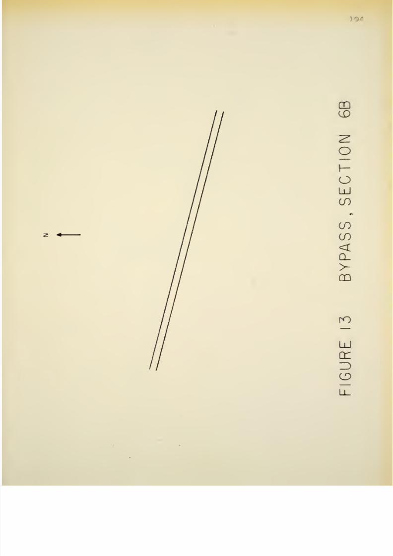
8/11/2019 Speed Delay
http://slidepdf.com/reader/full/speed-delay 118/141
CD
CD
O
o
LU
CO
CO
CO
<
CL
>
00
ro
LU
cr
O
l_L_
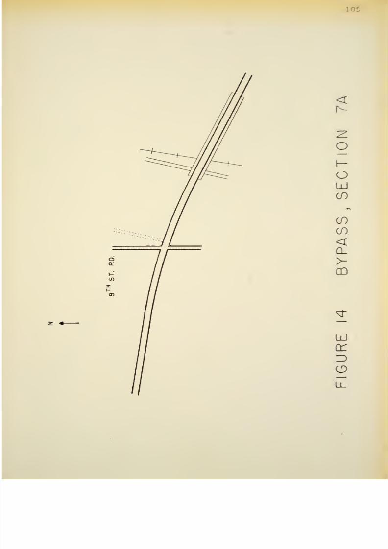
8/11/2019 Speed Delay
http://slidepdf.com/reader/full/speed-delay 119/141
10
<
O
o
LU
if)
CO
CO
<
Q_
>
CD
LU
cr
Z)
o
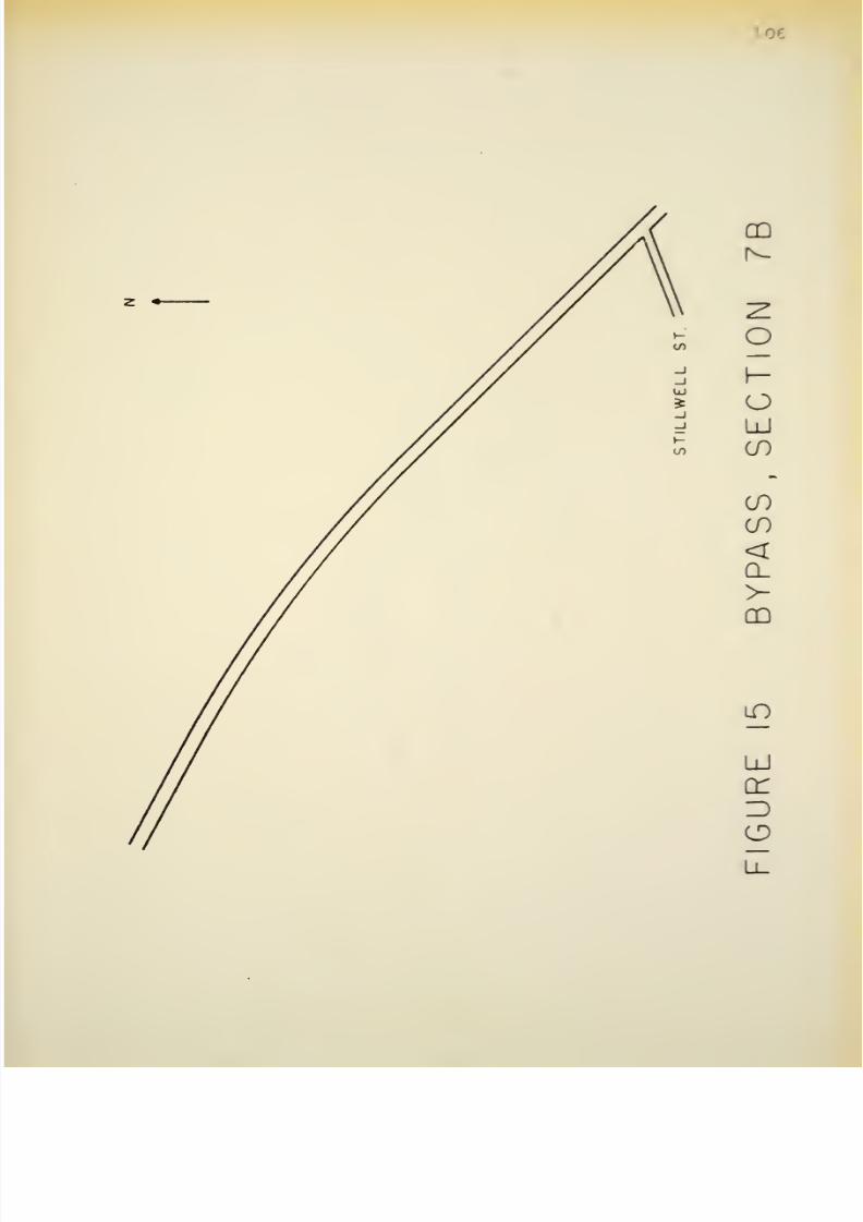
8/11/2019 Speed Delay
http://slidepdf.com/reader/full/speed-delay 120/141
CD
O
o
LU
CO
CO
CO
<
CL
DQ
LU
cr
CD
LL

8/11/2019 Speed Delay
http://slidepdf.com/reader/full/speed-delay 121/141
00
o
o
UJ
CO
00
CO
<
CL
>
00
LU
o

8/11/2019 Speed Delay
http://slidepdf.com/reader/full/speed-delay 122/141
•
08
2 *
<T>
O
O
Ld
V)
00
CO
<
CL
>
CD
LU
cr

8/11/2019 Speed Delay
http://slidepdf.com/reader/full/speed-delay 123/141
o
o
h-
o
LU
(f)
CO
CO
<
CL
>-
00
00
LU
cr
Ll
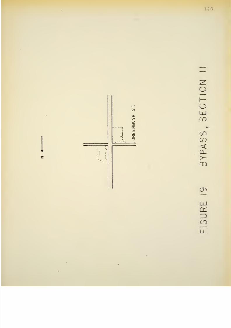
8/11/2019 Speed Delay
http://slidepdf.com/reader/full/speed-delay 124/141
:
LO
o
i-
U)
X
in
3
CD
1
z
1
Lu
D
Lu
IT
10
t
z
D
O
LU
CO
CO
CO
<
Q_
>
00
LU
DC
O

8/11/2019 Speed Delay
http://slidepdf.com/reader/full/speed-delay 125/141
Ill
t
z
D
1
1
- - -'
D
Di
CO
o
I—
o
LU
CO
if)
CO
<
CL
>-
00
O
CO
UJ
cr
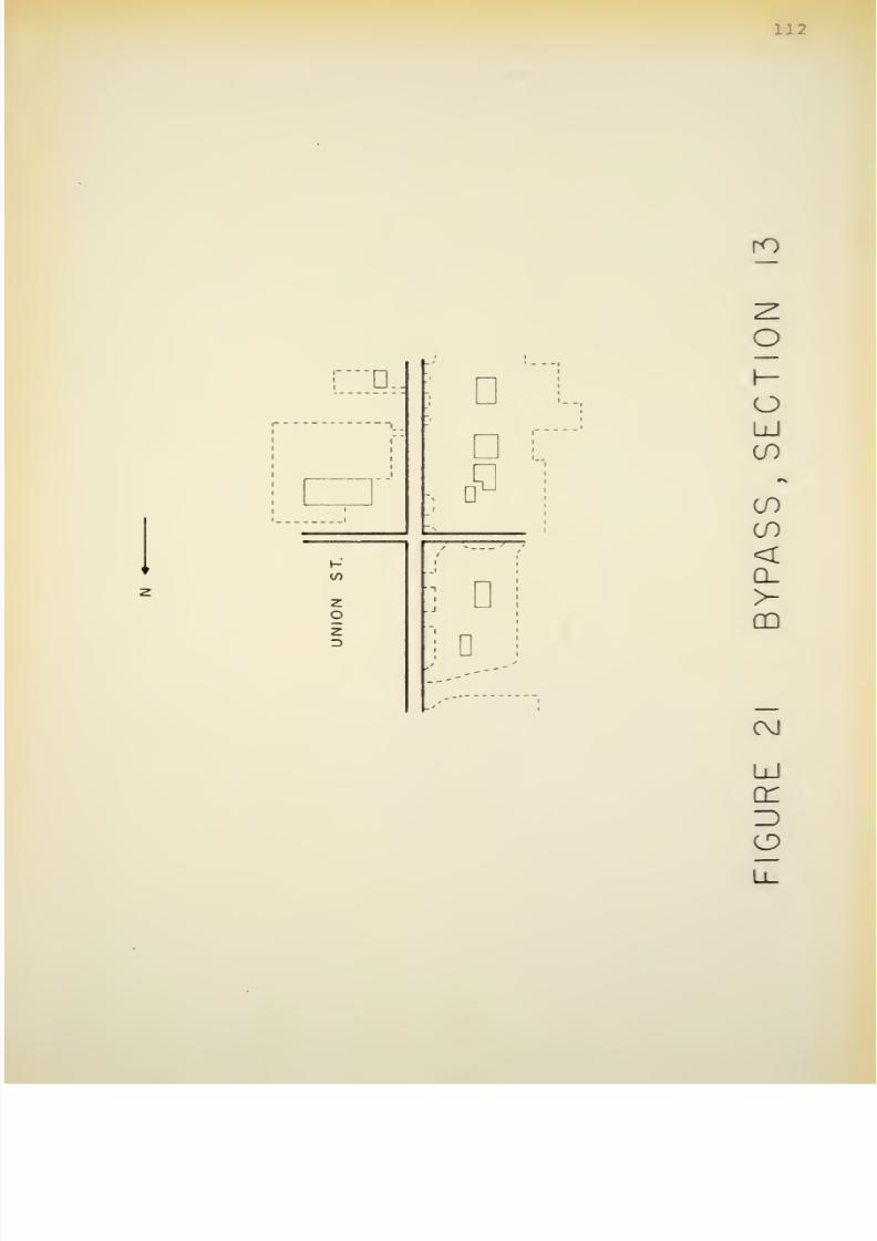
8/11/2019 Speed Delay
http://slidepdf.com/reader/full/speed-delay 126/141
112
D.
z
o
Z
3
D
D
D
.-
•--
.
]
i
I
D I
rO
O
O
LU
CO
CO
CO
<
CL
>
CM
LU
cr

8/11/2019 Speed Delay
http://slidepdf.com/reader/full/speed-delay 127/141
^r
D
/:.
O
O
LU
CO
.1
—
i
i
.
D'
C
a
\d
CO
CO
<
Q_
>-
CD
C\J
C\J
V.J.
_.-
Q
-=-.=
LU
cr
o
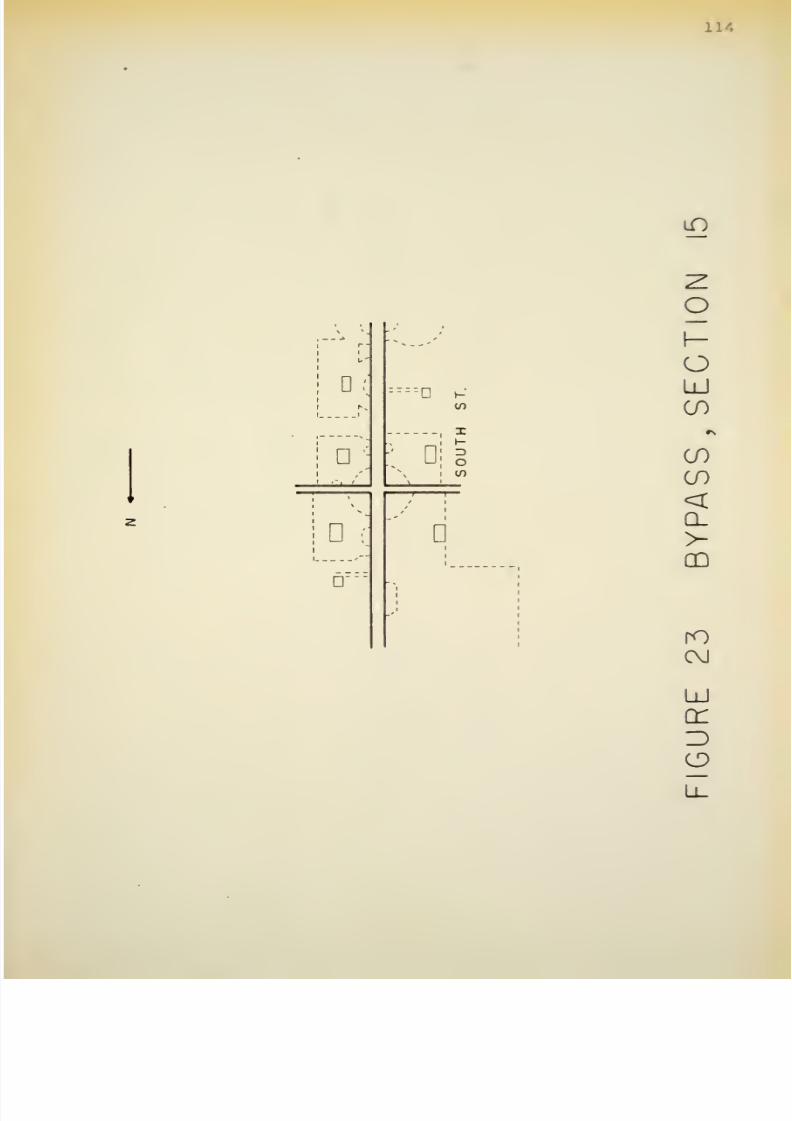
8/11/2019 Speed Delay
http://slidepdf.com/reader/full/speed-delay 128/141
114
D
:
,
'
'
•
•*
-''
:::
Z
D
1-
T
1-
'
u
3
O
\
(O
. . .
D
'
T
D
in
o
o
LU
CO
CO
CO
<
CL
>
QD
ro
cvi
UJ
cr
Ll
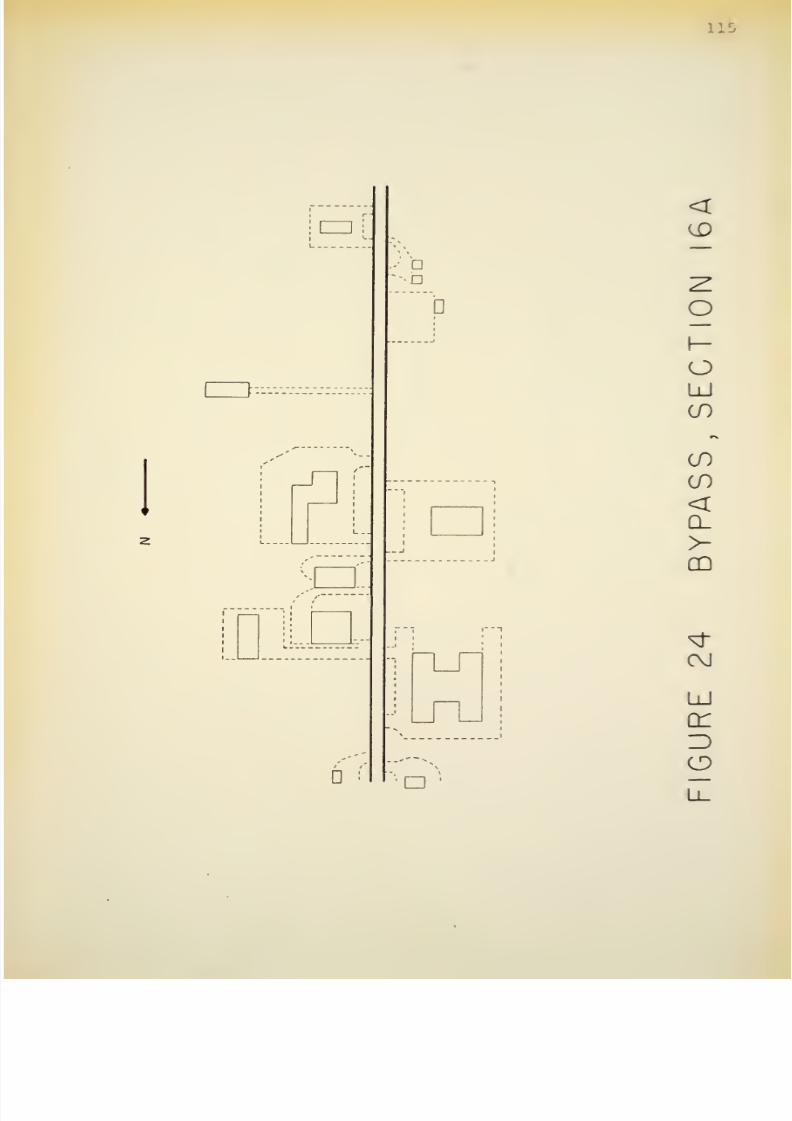
8/11/2019 Speed Delay
http://slidepdf.com/reader/full/speed-delay 129/141

8/11/2019 Speed Delay
http://slidepdf.com/reader/full/speed-delay 130/141
116
j
CD
CD
O
o
LU
CO
if)
if)
<
Q_
>
CD
D
to
to
to
o
in
CO
LU
O
LL.
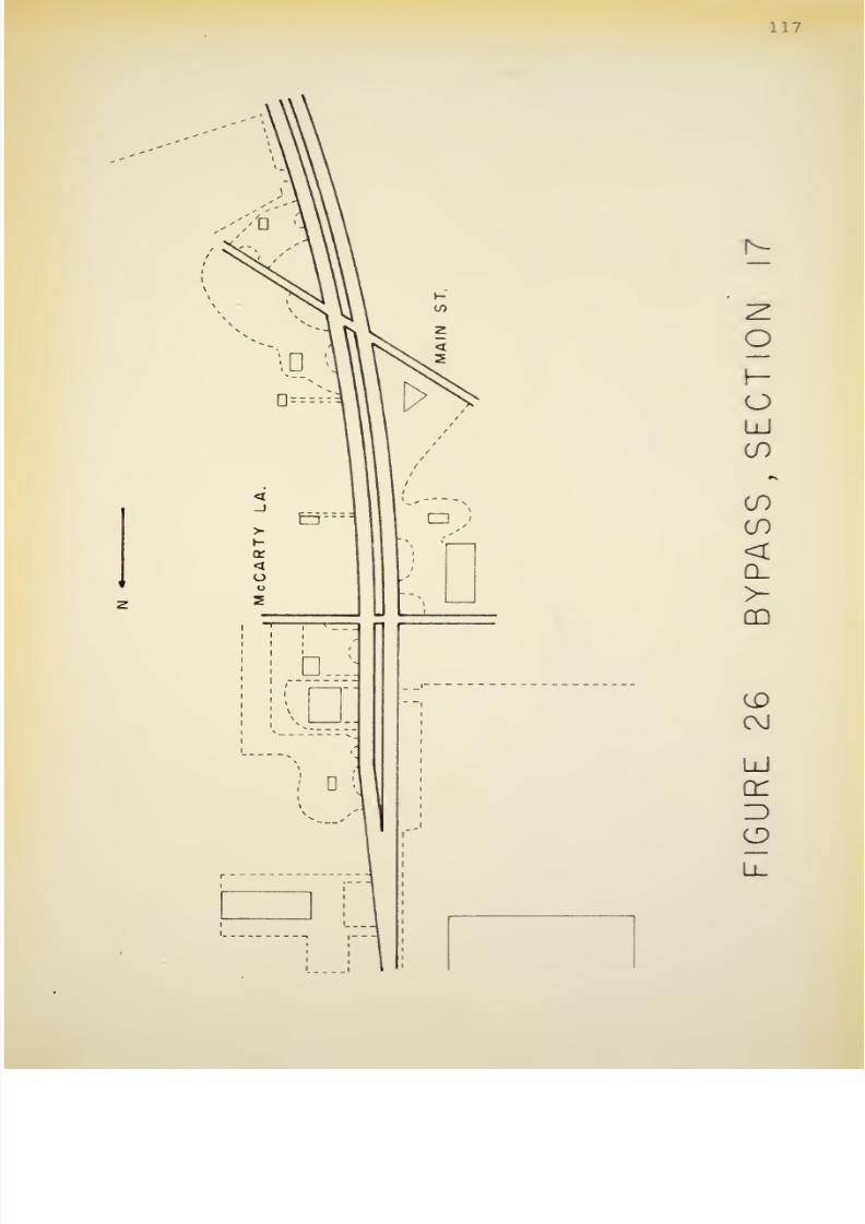
8/11/2019 Speed Delay
http://slidepdf.com/reader/full/speed-delay 131/141
117
2
N
O
o
LU
CO
if)
if)
<
CL
00
CD
00
Ld
Z>
if)
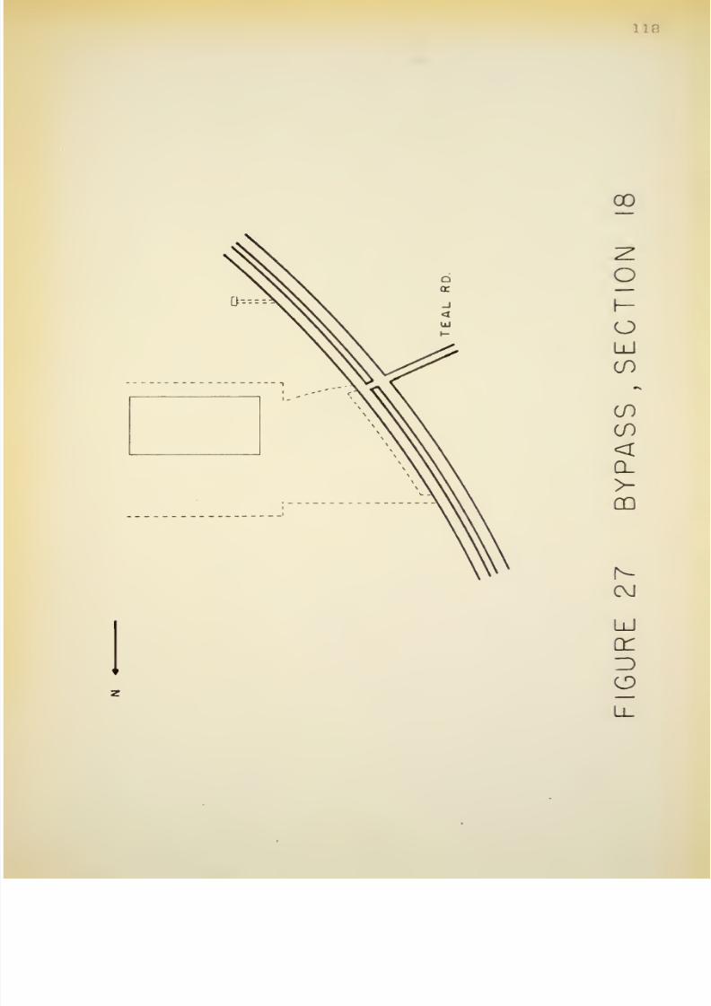
8/11/2019 Speed Delay
http://slidepdf.com/reader/full/speed-delay 132/141
I
L8
CD
O
o
Ld
CO
CO
CO
<
Q_
>-
GO
1^-
00
LiJ
cr
u_

8/11/2019 Speed Delay
http://slidepdf.com/reader/full/speed-delay 133/141
APPENDIX B
SUMMARY DaTA
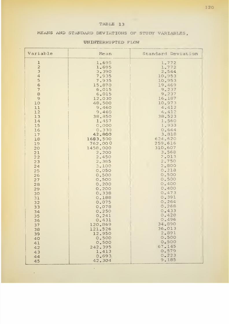
8/11/2019 Speed Delay
http://slidepdf.com/reader/full/speed-delay 134/141
120
TABLE
13
MEANS
AND
STANDARD
DEVIATIONS
OF
STUDY VARIABLES,
UNINTERRUPTED
FLOW
Variable
Mean Standard Deviation
1
2
3
4
5
6
7
8
9
10
11
12
13
14
15
16
17
18
19
20
21
22
23
24
25
26
27
28
29
30
31
32
33
34
35
36
37
38
39
40
41
42
43
44
45
1
1
3
7
7
15
6
6
12
48
9
9
38
1
42
1683
762
145?
2
2
2
120
121
12
242
1
42
.695
.695
.390
.935
.935
.870
.015
.015
.030
.500
.460
.460
.350
.457
.000
.330
.800
.500
.00
.000
.200
.450
.
385
.100
.050
.500
.500
.200
.200
.338
.188
.075
.078
.250
.241
.431
.869
.526
.950
.500
.500
.395
.413
.693
.304
1.
1.
2.
10.
10.
19.
9.
9.
16.
10.
4.
4.
38.
1.
1.
0.
3.
624.
259.
310.
.
2.
2.
o]
0.
0.
0.
:.
o.
0.
0.
0.
0.
0.
0.
34.
36.
2.
0.
0.
67.
0.
C
9,
772
772
544
953
95
3
469
237
237
187
973
412
412
523
560
933
644
818
620
616
607
568
013
750
300
213
500
500
400
400
47
3
391
264
268
433
428
496
890
013
891
500
500
145
5
-
^
223
185

8/11/2019 Speed Delay
http://slidepdf.com/reader/full/speed-delay 135/141
121
TABLE
14
CORRELATION
OF TRAVEL
SPEED
WITH
THE
OTHER
VARIABLES,
UNINTERRUPTED
PLOW
1
Correlation
Coefficient,
Travel
Speed
-0.169
-0.113
-0.196
-0.506
-0.468
-0.548
-C.512
-0.421
-0.5
32
+0.586
-0.340
-0.426
-0.074
+0.406
0.028
+0.032
-0.103
+0.064
-0.365
+0.224
-0.005
-0.208
0.158
-0.221
+0.255
-0.362
-0.429
-0.006
-0.081
+0.044
+0.067
-0.045
+0.077
+0.003
+0.063
-0.099
-0.527
-0.495
+0.087
-0.103
0.103
-0.539
-0.062
-0.503

8/11/2019 Speed Delay
http://slidepdf.com/reader/full/speed-delay 136/141
122
TiiliLL
15
CONTRIBUTIONS
OF
THE
13
PRINCIPAL
FACTOR
UNINTERRUPTED
FLOW
(Unities
in
Diagonal
of
Correlation
Matrix)
Factor
Eigenvalue
Percent
of
Cum.
Percent
of
Total
Variance
Total
Variar
A
7.63
20.01
20.01
B
6.63
17.52 37.5 3
C
3.86 10.16 47.69
D
2.54
6.69
54.38
E
2.08 5.48 59.86
F
1.88
4.94 64.80
G
1.61
4.22
69.02
H
1.50
3.96
72.98
I
1.32
3.46
76.44
J
1.20
3.17
79.61
K
1.14
2.99
82.60
L
1.12
2.94
85.54
M
1.01
2.68
68.22
1
1

8/11/2019 Speed Delay
http://slidepdf.com/reader/full/speed-delay 137/141
123
TaBLE
16
MEANS
AND
STANDARD
DEVIATIONS
OF
STUDY
VARIABLES,
INTERRUPTED
FLOW
Variable
Mean
Standard Deviation
46
0.200
0.400
47
0.100
0.300
48
0.100
0.300
49
482.600
371.428
50
377.000
218.327
51
0.401
1.558
52
-0.401
1.558
53
0.300
0.641
54
0.300
0.641
55
0.600
0.801
56
5.200
3.030
57
5.200
3.030
58
10.400
4.133
59
3.000
1.343
60
3.000
1.34
3
61
6.000
2.100
62
65.000
8.955
63
37.100
7.377
64
544.399
56.602
65
0.300
0.641
66
0.100 0.300
67
1.600
1.802
68
0.700
0.458
69
0.500
0.501
70
0.500
0.501
71
9.319
5.685
72
10.779
9.160
73
9.319
5.685
74
10.690
3.709
75
10.690 3.709
76
0.200
0.400
77
0.200
0.400
78
0.337
0.473
79
0.187
0.390
80
0.075 0.263
81
0.075
0.263
82
0.250
0.433
83
0.245
0.4
30
84
0.430
0.495
85
132.330
34.573
86
133.320
35.186
87
336.262
89.498
88
12.950
2.€
89
0.569
0.072
90
0.398
0.061
91
0.974
0.242
92
24.160
10.166

8/11/2019 Speed Delay
http://slidepdf.com/reader/full/speed-delay 138/141
TABLE
17
124
CORRELATION OF TRAVEL
SPEED
AND DELAY WITH
THE
OTHER VARIABLES, INTERRUPED
FLOW
Variable
46
47
48
49
50
51
52
53
54
55
56
57
58
59
60
61
62
63
64
65
66
67
68
69
70
71
72
73
74
75
76
77
78
79
80
81
82
83
84
85
86
87
88
89
90
91
Correlation Coefficient
Travel
Speed
+0.271
+0.106
-0.139
-0.085
0.102
-0.127
-0.122
+0.003
+0.088
+0.073
-0.071
-0.003
-0.054
+0.033
+0.103
+0.087
-0.237
-0.056
+0.096
+0.190
-0.139
-0.200
+0.028
-0.114
+0.114
+0.018
-0.101
-0.140
+0.131
-0.173
+0.020
-0.074
+0.027
+0.090
-0.100
+0.127
+0.001
+0.028
-0.092
-0.180
-0.225
-0.244
+0.112
+0.190
+0.135
-0.223
Delay
-0.175
-0.110
+0.177
+0.177
-0.047
+0.122
+0.126
+0.065
-0.017
+0.038
-0.007
-0.046
-0.039
-0.053
-0.111
-0.105
+0.157
-0.028
-0.144
-C.157
+0.177
+0.188
-0.021
+0.135
-0.135
-0.053
+0.106
+0.135
-0.164
+0.192
-0.035
+0.097
-0.048
-0.071
+0.097
-0.084
-0.012
-0.037
+0.088
+0.091
+0.149
+0.139
-0.102
-0.229
-0.112
+0.147

8/11/2019 Speed Delay
http://slidepdf.com/reader/full/speed-delay 139/141
Table
18
contributions of
the
11
principal factor
interruptej flow
(Unities
in
Diagonal
of
Correlation
Matrix)
Factor
Eigenvalue
Percent
of
Cum. Percent of
Total Variance
Total
Variance
N
7.61 18.57
18.57
6.09
14.85 33.42
P
5.81
14.17
47.59
Q
3.90
9.50 57.
R
3.22
7.86
64.95
S
2.57
6.27
71.22
T
2.07
5.06
76.23
U
1.95
4.76
81.04
V
1.50
3.67
84.71
W
1.19
2.90
87.61
X
1.10
2.68
90.29

8/11/2019 Speed Delay
http://slidepdf.com/reader/full/speed-delay 140/141

8/11/2019 Speed Delay
http://slidepdf.com/reader/full/speed-delay 141/141