Spin Connection Resonance in the Bedini

Machine

by

Myron W. Evans,Civil List Scientist,

Treasury(emyrone@aol.com)

H. Eckardt, C. Hubbard, J. Shelburne,Alpha Institute for Advanced Studies (AIAS)(www.aias.us, www.atomicprecision.com)

Abstract

Spin connection resonance (SCR) is used to explain theoretically why devicesin electrical engineering can use the properties of space-time to induce voltage.Einstein Cartan Evans (ECE) theory has shown why classical electrodynamicsis a theory of general relativity in which covariant derivatives are used with thespin connection playing a central role. These concepts are applied to a deviceknown as the Bedini machine.

Keywords: Spin connection resonance, electrodynamics in general relativity,Einstein Cartan Evans theory, Bedini machine.

1 Introduction

Recently [1]- [10] the Einstein Cartan Evans (ECE) �eld theory has been gen-erally accepted as the �rst successful uni�ed �eld theory on the classical andquantum levels. It shows that classical electrodynamics is a theory of generalrelativity, not of special relativity. In ECE theory the spin connection plays acentral role in the structure of the laws of electrodynamics and in the way theelectric and magnetic �elds are related to the scalar and vector potentials. TheECE equations of classical electrodynamics allow the existence of resonancesin potential which can be used to extract electric power from the structure ofspace-time. This structure is not the vacuum, the latter in relativity theoryis a universe devoid of all curvature and torsion. The resonance phenomenoninduced by these equations is known as spin connection resonance (SCR). Inthis paper it is applied to a device known as the Bedini machine [11], which hasbeen patented and which has been shown to be experimentally reproducible and

1

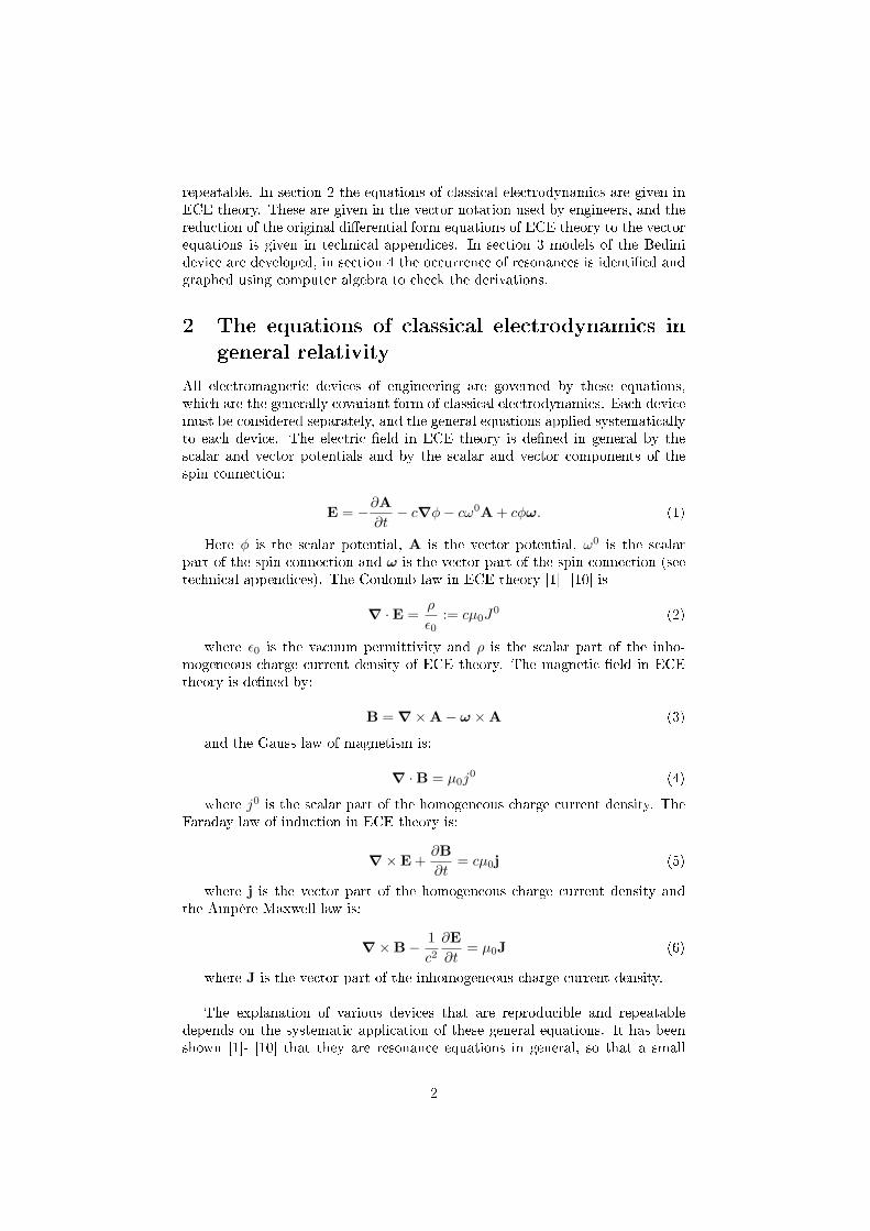
repeatable. In section 2 the equations of classical electrodynamics are given inECE theory. These are given in the vector notation used by engineers, and thereduction of the original di�erential form equations of ECE theory to the vectorequations is given in technical appendices. In section 3 models of the Bedinidevice are developed, in section 4 the occurrence of resonances is identi�ed andgraphed using computer algebra to check the derivations.

2 The equations of classical electrodynamics in

general relativity

All electromagnetic devices of engineering are governed by these equations,which are the generally covariant form of classical electrodynamics. Each devicemust be considered separately, and the general equations applied systematicallyto each device. The electric �eld in ECE theory is de�ned in general by thescalar and vector potentials and by the scalar and vector components of thespin connection:

E = −∂A∂t− c∇φ− cω0A + cφω. (1)

Here φ is the scalar potential, A is the vector potential, ω0 is the scalarpart of the spin connection and ω is the vector part of the spin connection (seetechnical appendices). The Coulomb law in ECE theory [1]- [10] is

∇ ·E =ρ

ε0:= cµ0J

0 (2)

where ε0 is the vacuum permittivity and ρ is the scalar part of the inho-mogeneous charge current density of ECE theory. The magnetic �eld in ECEtheory is de�ned by:

B = ∇×A− ω ×A (3)

and the Gauss law of magnetism is:

∇ ·B = µ0j0 (4)

where j0 is the scalar part of the homogeneous charge current density. TheFaraday law of induction in ECE theory is:

∇×E +∂B∂t

= cµ0j (5)

where j is the vector part of the homogeneous charge current density andthe Ampère Maxwell law is:

∇×B− 1c2∂E∂t

= µ0J (6)

where J is the vector part of the inhomogeneous charge current density.

The explanation of various devices that are reproducible and repeatabledepends on the systematic application of these general equations. It has beenshown [1]- [10] that they are resonance equations in general, so that a small

2

driving term can produce a very large ampli�cation of space-time e�ects throughthe inter-mediacy of the spin connection. Devices which �nd no explanation inthe standard model can be explained in this way. For example, we considerthe Bedini device [11] as one in which an electric pulse produced by the rateof change of a magnetic �eld is induced in a generator. The electric �eld pulseproduces a pulse of electrons in a battery [11] as controlled by Eqs. (1) and (2),from which:

∇ ·∇φ+1c

∂

∂t(∇ ·A) + ∇ ·

(ω0A

)−∇ · (φω) = −µ0J

0. (7)

This equation produces resonances in two ways, each of which gives a reso-nance equation.

1. If it is assumed that the origin of E is purely due to φ, we obtain the basicresonance equations of paper 63 and 92 of the ECE series [1]- [10].

2. If it is assumed that the origin of E is purely magnetic, and that the scalarpotential is zero, we have:

1c

∂

∂t(∇ ·A) + ∇ ·

(ω0A

)= −µ0J

0. (8)

i.e.

∇ ·(

1c

∂A∂t

+ ω0A)

= −µ0J0. (9)

which can be integrated to give a resonance equation. It is also possibleto produce a time dependent resonance equation from Eqs. (1) and (6). TheAmpère Maxwell law (6) is considered to produce a driving term:

∂E∂t

= c2 (∇×B− µ0J)driving = −∇∂φ

∂t− ∂

2A∂t2− ∂

∂t

(cω0A

)+∂

∂t(cφω) (10)

so that the most general resonance equation of time-dependent type is:

∂2A∂t2

+ c∂ω0

∂tA + cω0 ∂A

∂t= c

∂φ

∂tω + cφ

∂ω

∂t+ c2µ0J−∇∂φ

∂t− c2∇×B. (11)

If there is no charge and current density this equation reduces to:

∂2A∂t2

+ cω0 ∂A∂t

+ c∂ω0

∂tA = −c2 (∇×B)driving . (12)

There is resonance in A under the following conditions:

1. the scalar part, ω0, of the spin connection is non-zero,

2. the time derivative, ∂ω0

∂t , is non-zero,

3. the curl ∇×B is non-zero and also time dependent.

3

When investigating various claims such as the Bedini machine it is necessaryto use equations such as this, which show for example that the magnetic �eld inthe design must be both space and time dependent, and produced by a devicethat satis�es these requirements. That is an example of a design prediction ofECE theory in engineering.

In addition to Eq. (6) there exists the Coulomb law (2), which is the reso-nance equation [1]- [10]:

∇ ·(cφω −∇φ− ∂A

∂t− cω0A

)=

ρ

ε0. (13)

In the absence of charge this equation reduces to:

∇ ·(∂A∂t

+ cω0A)

= 0 (14)

so ω0 may be eliminated between equations (12) and (14). Eq. (14) is:

∇ · ∂A∂t

= −c(A ·∇ω0 + ω0∇ ·A

). (15)

Therefore ω0 is governed by Eqs. (12) and (15) which must be solved simulta-neously. The latter equation can be integrated with the divergence theorem [12].For any well behaved vector �eld V(r) de�ned with a volume surrounded by aclosed surface S: ∮

S

V · n da =∫V

∇ ·V d3r. (16)

Thus for the Coulomb law 12:∫V

(∇ ·E− ρ

ε0

)d3r = 0 (17)

i.e. ∮S

E · n da =1ε0

∫V

ρ(r) d3r. (18)

So the integration of Eq. (14) is:∮S

(∂A∂t

+ cω0A)· n da = 0 (19)

i.e. ∮S

∂A∂t· n da = −c

∮S

ω0A · n da. (20)

Eq. (20) is a relation between ω0 and A. The correct way of solving (12)is simultaneously with (18). This can be carried out numerically for variousmodels of ∇ × B produced by various devices. It can be seen that ω0 canbe eliminated and that Eq. (12) reduces to an undamped oscillator [1]- [10]because ∂A

∂t is eliminated in favour of A. So in this example A can be ampli�edto INFINITY for various models of ∇ ·B acting as a driving force. There is noneed to model ω0 because it can be expressed in terms of A.

4

3 Systematic evaluation of equations for the Be-

dini machine

If no scalar potential is present, the ECE �eld equations (1-6) in the base man-ifold take the simple form:

∇×E + B = 0 (21)

∇×B− 1c2

E = 0 (22)

∇ ·B = 0 (23)

∇ ·E = 0 (24)

with the de�nition equations

B = ∇×A− ω ×A (25)

E = −A− c ω0A. (26)

Here the dot denotes the time derivative, A is the vector potential, ω thevector spin connection and ω0 the scalar spin connection, both in units of 1/m.It is more convenient to transform the scalar spin connection to a time frequency:

ω0 := c ω0. (27)

Eqs. (21-24) represent a system of eight equations and by the right-handside of Eqs. (25-26) seven variables are de�ned. In the most general case thescalar potential Φ is the eights variable so that (21)-(24) can be solved uniquely.Here we restrict consideration to the case without charges and therefore withouta scalar potential.

In classical electrodynamics we have the same equations, but without thespin connection. This leads to an inconsistency for solving the equations. Some-times solely the �elds E and B are considered, then only the equations (21)-(22)can be used. The Gauss and Coulomb law are tried to be handled as �con-straints�, but this leads to an over-determined equation system. In other cases(when charges and currents are present) the potentials A and Φ are taken asvariables. Then only the Eqs. (22) and (24) can be used, the other two arehomogeneous and lead to the trivial solution A = 0. In contrast, ECE the-ory presents a perfectly well-de�ned situation with eight equations and eightvariables.

There are basically two methods to combine these equations to obtain reso-nances for particular cases:

1. use (21) and (22) completely to de�ne driving terms, use (25) and (26) asbasis for resonance solutions,

2. use the terms B, E in (21), (22) as driving terms, insert curl of (25) and(26) into (21) and (22) and use these equations for resonance solutions.

5

We will see that both methods are not applicable in all possible cases.In addition to both methods, we have to use one of the equations (3), (4).

The actual choice depends on the case if ω or ω0 occurs in the equations (21)and (22). In the following we work out the distinguished cases 1 and 2 each forEq. (21) (called sub-case a) and Eq. (22) (called sub-case b).

1a: Faraday Law as driving term, B �eld resonance

By de�nition we have

(∇×E)driving = −(B)driving (28)

Inserting the time derivative of (25) into (28):

∇× A− ω ×A− ω × A = (B)driving = −(∇×E)driving (29)

In order to obtain resonance a di�erential equation of second order in timeis required, therefore we take a further time derivative:

∇× A− ω ×A− 2ω × A− ω × A = (B)driving (30)

This is a resonance equation in A (for constant ω) as well as in ω (for con-stant A). The spin connection can be obtained from simultaneously solving Eq.(23). This could be su�cient, if not all components of A or ω are di�erent fromzero. In the most general case further equations have to be added.

1b: Ampère-Maxwell Law as driving term, E �eld resonance

In analogy to case 1a we obtain from (22):

(∇×B)driving =1c2

(E)driving (31)

and by applying (26):

A + ω0A + ω0A = −(E)driving (32)

This is an equation for a damped resonance for ω0 > 0. The spin connectioncan be determined by combining (32) with (24).

2a: B �eld de�nition as driving term, Faraday Law as resonance

equation

Taking the magnetic �eld in (21) as driving term gives

∇×E = −(B)driving. (33)

Inserting (26) into (33):

∇× A + ∇× (ω0A) = (B)driving (34)

or after taking a further time derivative:

∇× A + ∇× (ω0A) + ∇× (ω0A) = (B)driving (35)

which is the equivalent of (30) with the other type of spin connection.

6

2b: E �eld de�nition as driving term, Ampère-Maxwell Law as reso-

nance equation

Starting with Eq. (22) we obtain

∇×B =1c2

(E)driving (36)

and with (25):

∇×∇×A−∇× ω ×A =1c2

(E)driving (37)

or

∇ (∇ ·A)−∇2A−ω (∇ ·A)+A (∇ · ω)−(A ·∇) ω+(ω ·∇) A =1c2

(E)driving.

(38)This is a resonance equation for the space coordinates of A. Investigating

time-dependent resonances requires a twofold additional time derivation whichmakes this equation impractible.

4 Detailed investigation of the Bedini Machine

4.1 Description of the Bedini machine

In the book "Free Energy Generation" [13], see also [14], Bedini explains hisbattery charging device of 1984. He presents some variants of the machineconstructed within 20 years. The basic design has remained the same. Thepatented Bedini machine inventor claims that his machines are able to extractenergy from the surrounding space in the form of radiant energy. The authorshere attempt to show that the energy produced by these machines is the result ofdisturbing the local space-time unit volume, creating a resonance e�ect, whichallows energy to �ow out of the local unit volume, in the form of asymmetricelectromagnetic wave forms into a recti�er circuit, where it can be then sent toa storage device. The mathematical expressions developed are based on ECE�eld theory. The resulting expressions will allow electrical designers to produceproductive circuits, based on this math, since the inventor has not furnishedan adequate explanation of the machines' operation. One of the authors hasreplicated two of the Bedini machines successfully, and others have had successbuilding and operating the machines.

The Bedini machine has several distinct elements (see Fig. 1). The inputpower supply, which can be a battery or a recti�ed power supply from an externalsupply, provides the transducer coil and trigger circuitry with energy to pulsethe unit volume through the trigger winding.

The magnet induces an asymmetric pulse into the transducer core, whichinduces an e-m pulse in the trigger winding, power winding, and generatorwinding. The trigger pulse causes power to �ow into the power winding, givinga boot to the magnet as it goes on by, thereby powering the rotor to the nextmagnet. The transducer pulse from the coils �ows into the unit volume, up-setting the local �eld, and the resulting return energy is recti�ed after �owingthrough the generator winding.

7

Figure 1: Bedini machine (from [13], p. 47).

All of these windings of the transducer are separate coils, wound concentri-cally on a spool, which has a core consisting of mild iron rods, typically 1/16"in diameter. Once the rotor is spun manually, and the power source and storagedevice are connected, the rotor will accelerate to a select speed determined bya tuning rheostat, and the machine will maintain that speed inde�nitely, charg-ing the storage device, using less energy to run than it stores, thereby achievingover unity in its operation. One of the authors has determined that the machineoperates more e�ciently at 24 Volts DC, than at 12 Volts DC, and the machineoperates at almost twice the rpm as compared to 12 Volt operation.

Mr. Bedini has built several demonstrator machines in the kilowatt size,however, one of the authors' machines is only capable of 10-15 watts of output,but this size is adequate to provide meaningful test results. One of the authorsis presently building a larger machine to replicate Mr. Bedini's claims of higherpower outputs. In addition to the rotor style machines, the inventor has shownsolid state designs, which the authors have not replicated yet, but others have,with limited output success. A company using Mr. Bedini's designs is presentlymarketing a line of battery chargers claiming to use radiant energy to enhancebattery life and longevity.

8

4.2 Models of the Bedini machine

Charging of a battery means a �ow of ions in the electrolyte in direction reverseto the discharging current. According to the explanations of Bedini, the batterycharging process is evoked by high frequency pulses. This type of charging iscompletely di�erent from the conventional DC charging process where the iontransport is e�ected by applying a DC voltage. Bedini points out that the highfrequency / high voltage oscillations initiate a coupling to spacetime so that theions resonate and move in the direction opposite to the discharge current. Nosigni�cant conventional recharging energy has to be expended in this process.

Key of understanding the process is the mechanism of tapping the vacuumbackground energy, i.e. to evoke a resonant coupling to the spacetime back-ground. As has been shown by ECE �eld theory [papers 63, 92], a coupling tospacetime background can be achieved by a resonance circuit. Such an originalcircuit from Bedini is shown in Fig. 1.

The key component of the Bedini machine is the tri�lar wound coil whichacts as a combined transmitter-receiver transducer. In the following we use theworking hypothesis that the spacetime coupling takes place by means of thiscoil. Therefore we need not consider the complex electro-chemical processes inthe battery, and an electrical potential Φ can be omittet as already done inEquations (21-26).

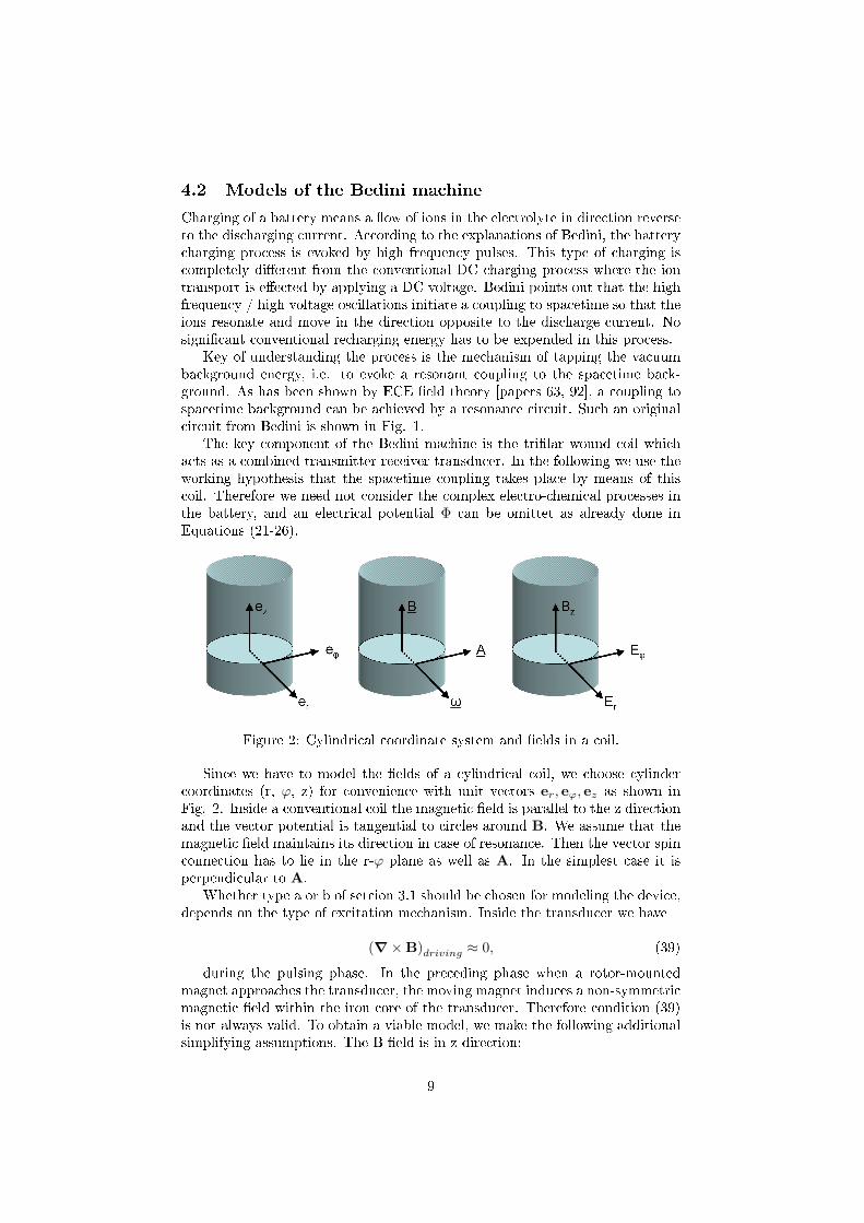
Figure 2: Cylindrical coordinate system and �elds in a coil.

Since we have to model the �elds of a cylindrical coil, we choose cylindercoordinates (r, ϕ, z) for convenience with unit vectors er, eϕ, ez as shown inFig. 2. Inside a conventional coil the magnetic �eld is parallel to the z directionand the vector potential is tangential to circles around B. We assume that themagnetic �eld maintains its direction in case of resonance. Then the vector spinconnection has to lie in the r-ϕ plane as well as A. In the simplest case it isperpendicular to A.

Whether type a or b of setcion 3.1 should be chosen for modeling the device,depends on the type of excitation mechanism. Inside the transducer we have

(∇×B)driving ≈ 0, (39)

during the pulsing phase. In the preceding phase when a rotor-mountedmagnet approaches the transducer, the moving magnet induces a non-symmetricmagnetic �eld within the iron core of the transducer. Therefore condition (39)is not always valid. To obtain a viable model, we make the following additionalsimplifying assumptions. The B �eld is in z direction:

9

B =

00Bz

. (40)

The vector potential in classical electrodynamics then has only a ϕ and rcomponent:

A =

ArAϕ0

. (41)

Since the spin connection ω cannot be in parallel to A and B according toEq. (25), we choose

ω =

ωrωϕ0

. (42)

Due to the rotational symmetry of the device, there cannot be a ϕ depen-dence of the �elds. In total we have the functional dependencies

Bz = Bz(r, t)Ar = Ar(r, t)Aϕ = Aϕ(r, t)ωr = ωr(r, t)ωϕ = ωϕ(r, t)ω0 = ω0(r, t)

(43)

With (40-42) we have (using the di�erential operators in cylinder coordi-nates)

∇×A =

00

1r∂∂r (rAϕ)− ∂Ar

∂ϕ

, (44)

ω ×A =

00

ωrAϕ − ωϕAr

. (45)

The divergence of a vector V is in cylindric coordinates:

∇ ·V =1r

∂

∂r(rVr) +

1r

∂

∂ϕ(Vϕ) +

∂

∂z(Vz) . (46)

We are now ready to apply the methods 1a, 1b, 2a. Starting with 1a, weobtain from Eq. (30) with the special form of A and ω (40-45):

1r

∂

∂r(rAϕ)− ∂Ar

∂ϕ−ωrAϕ+ωϕAr−2(ωrAϕ−ωϕAr)−ωrAϕ+ωϕAr = (Bz)driving

(47)From (23) follows

∇ · (∇×A− ω ×A) = 0 (48)

10

or

∂

∂z

(1r

∂

∂r(rAϕ)− ωrAϕ + ωϕAr

)= 0. (49)

This equation is trivially ful�lled. Even if we additionally assume Ar =ωϕ = 0 we have one equation with two unknowns Aϕ and ωr so that no uniquesolution is obtained.

Considering the alternative case 2a we get from Eq. (35):

1r

∂

∂r

(rAϕ + rω0Aϕ + rω0Aϕ

)− ∂

∂ϕ

(Ar + ω0Ar + ω0Ar

)= (Bz)driving. (50)

From Eq. (24) follows

∇ ·(−A− ω0A

)= 0 (51)

or1r

∂

∂r

(rAr + rω0Ar

)+

1r

∂

∂ϕ

(Aϕ + ω0Aϕ

)= 0 (52)

According to (43) Eqs. (50) and (52) can be simpli�ed to

1r

∂

∂r

(rAϕ + rω0Aϕ + rω0Aϕ

)= (Bz)driving (53)

1r

∂

∂r

(rAr + rω0Ar

)= 0 (54)

These are two equations for three unknowns and not unique as before.Finally we apply case 1b. This is di�erent from the previous ones since the

electrical �eld is considered to be the driving term. From Eq. (32) we obtainthe two equations

Ar + ω0Ar + ω0Ar = −(Er)driving (55)

Aϕ + ω0Aϕ + ω0Aϕ = −(Eϕ)driving (56)

and from Eq. (24):

1r

∂

∂r

(rAr + rω0Ar

)= 0 (57)

or

Ar +(ω0 + r

∂ω0

∂r

)Ar + r

∂Ar∂r

+ rω0∂Ar∂r

= 0. (58)

We see that the spin connection is coupled to the radial part of the vectorpotential. This indicates that the unit volume interacting with spacetime maybe somewhat extended beyond the transducer. The occurrence of E implies anon-vanishing curl of B according to (31).

The result (57) can further be simpli�ed by applying the divergence theoremas explained at the end of section 2. The surface integral of Eq. (19) is to betaken over the cylinder surface of the model. The parts over the circular areascancel out due to the assumed symmetry in z direction. For the cylindrical partthe ϕ component of the vector potential is perpedicular to the surface normal

11

and does not contribute anything. The only contributing part is the radialcomponent: ∫

V

∇ ·Ad3r =∫S

(Ar + ω0Ar)da = 0 (59)

SinceAr and ω0 are independent on the individual surface points, the integralcan be evaluated trivially and results in

ω0 = − ArAr

. (60)

The equations (55, 56, 60) are three equations for three unknowns Ar, Aϕ,ω0. This set of equations has to be solved numerically to provide guidanceto designers in sizing the transducer, designing the trigger and power circuits,and predicting power outputs. Since the unit volume is surrounded by thelarge number of unit volumes in a spherical con�guration(the rest of space), thetheoretical power input to the machine transducer is limited by its conductorsize and impedance seen looking into the transducer from the space side.

This paper discusses the Bedini machine in particular, but the concept of atransducer acting as a transmitter-receiver for power extraction from the sur-rounding space should be applicable to other machine designs also.

The inventor has put forth a hypothesis as to how his machines operate,which is non-conventional in its premise. The authors here suggest that thelatest ECE theory will provide a rational explanation to the machines' operation,using conventional mathematical notation, and recognized physical theory.

4.3 Resonance behaviour of the vector potential

Without doing any numerical calculations, we can demonstrate that resonancesolutions for Eqs. (55, 56) exist. We assume a harmonic time dependence

Ar = A1(r) sin(ωt) (61)

ω0 = ω1(r) sin(ωt) (62)

with a frequency ω (not to be confused with the spin connection ω0) andradius dependent functions A1 and ω1. Let's further denote the right-hand sideof (55) by f1, then this equation can be written:

2A1ω1ω cos(ωt) sin(ωt)−A1ω2 sin(ωt) = −f1. (63)

For ωt = π/4 we have

sin(ωt) = cos(ωt) =1√2

(64)

and (63) simpli�es to

A1(ω1ω −ω2

√2

) = −f1 (65)

which gives the solution for Ar:

12

A1 =f1

ω2√2− ω1ω

. (66)

There is resonance when the denominator approaches zero, i.e.

ω1 =ω√2. (67)

If we had de�ned (61,62) by the cosine function, we had got the same valuefor ω0 with a negative sign. From this simple model we learn that the spinconnection can assume both signs (in contrast to a real frequency) and show upsharp resonances for certain phases of the time period. This is in accordancewith the experimental �ndings. From the original Eqs. (55,56) we would expecta damped oscillation, but these equations are non-linear and therefore someunexpected results can occur, in this case an undamped oscillation.

4.4 Computation of the energy balance

The theory should provide a method to estimate the energy balance of theBedini machine. According to the previous section it is assumed that the excessenergy comes from the spacetime processes in the extended unit volume, wherethey are evoked by the transducer. So a calculation has to compare the energydensity of the input �elds (E)driving or (B)driving to the energy of the total�elds being present in the resonance case. The result may depend on whetherwe consider the energy of the force �elds only or whether we include the e�ectson the spacetime potential A. In the �rst case we can de�ne the energy densitiesfor input and output:

uin =ε02

(E2)driving +1

2µ0(B2)driving, (68)

uout =ε02

E2 +1

2µ0B2. (69)

The resulting total energies then are obtained by integrating over the unitvolume and time:

Ein =∫uin d

3r dt (70)

Eout =∫uout d

3r dt (71)

and the �coe�cient of performance� is

COP =EoutEin

. (72)

Alternatively, the output energy can be related to the spacetime potential.From the minimal prescription of momentum density p

p→ p+ eA (73)

we can de�ne the kinetic energy density of the �eld by

13

u =e2A2

2m(74)

where m is the �mass� of the �eld volume. According to the de Broglieequation

m =~ωc2

(75)

the mass corresponds to a frequency ω. This leads to the expression

u = uout =e2c2

2~ωA2. (76)

4.5 Analytical and numerical solutions

The equations to be solved for the model we have developed (Eqs. 55, 56, 60)read

Ar + ω0Ar + ω0Ar = −f1 (77)

Aϕ + ω0Aϕ + ω0Aϕ = −f2 (78)

ω0 = − ArAr

. (79)

with driving terms f1(r) and f2(r). Instead of Eq. (79) we can alternativelyuse its original form (58) without application of the divergence theorem:

Ar +(ω0 + r

∂ω0

∂r

)Ar + r

∂Ar∂r

+ rω0∂Ar∂r

= 0. (80)

The di�erence is that the original form represents a di�erential equation inr while the r di�erentiation has vanished in the other form. Thus Eqs. (77-79)are only to be solved in the time domain which is a great alleviation. In thiscase Eq. (79) can be inserted into (77). Then all terms on the left cancel out,leading to the condition

f1 = 0. (81)

Obviously this is a compatibility condition, indicating that a driving forcef1 cannot be applied. The second Equation (78) can be solved analytically bycomputer algebra and gives the particular solution

Aϕ = ω0 f2

(e−ω0 t

∫eω0 t

ω0 ω0 t− ω0 + ω20

dt−∫

1ω0 ω0 t− ω0 + ω2

0

dt

)(82)

As already made plausible in section 4.3, this is a resonance equation if thedenominator goes to zero. This means that resonances occur at solutions of thedi�erential equation

ω0 ω0 t− ω0 + ω20 = 0. (83)

Computer algebra gives for this equation the general solution

14

ω0 t− log (ω0) = c (84)

with a constant c. This is a transcendent equation for ω0. Since c is arbitrary,there is an in�nite number of resonances in the whole interval of real numbersfor ω0.

All further investigations are made by a numerical model. As we have seen byanalysing Eq. (77) the vector potential Ar can be chosen freely. Considering theBedini machine, such a radial component can only be created by an asymmetricdisturbance of the �eld potential of the transducer coil. This is achieved bythe magnets of the wheel passing the transducer. We model these pulses by asinoidal function:

Ar(t) = A1 sin6(ωt) (85)

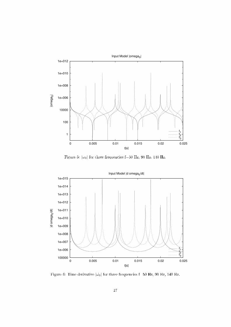
with an arbitrary amplitude A1 and a time frequency ω. This function andits time derivative are shown in Figs. 3 and 4 for three frequencies. With thisansatz, Eq. (79) takes the form

ω0(t) = −6ω cot(ωt). (86)

This function has vertical tangents where the values approach in�nity, seeFig. 5 for a plot of |ω0| for three frequencies in a logarithmic scale. Consequently,the derivative shows also this behaviour (Fig. 6).

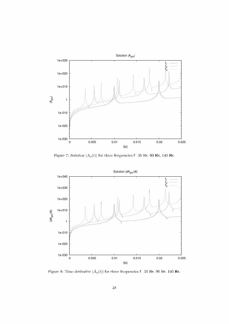
Eq. (78) has been solved numerically for Aϕ. The driving force f2 wasassumed to be in proportion to the �symmetry breaking� potential Ar. Withω0 having the singular behaviour, the solution spans a remarkable order ofmagnitude and is vulnerable to numerical instabilities. Therefore the solutionwas checked by inserting it back into Eq. (78) and checking for equality with f2.In all cases the equality was maintained within su�cient precision. The result(Fig. 7) shows giant resonance peaks over 15 orders of magnitude which occurin coincidence with the structure of ω0. Obviously these peaks correspond tothe peak signals in the Bedini machine. The time frequency is to be identi�edwith the passing rate of the magnets over the transducer. To make comparisoneven more appropriate, in Fig. (8) the derivative of Aϕ is shown which shouldcorrespond to the induced voltage

Uind = −Aϕ. (87)

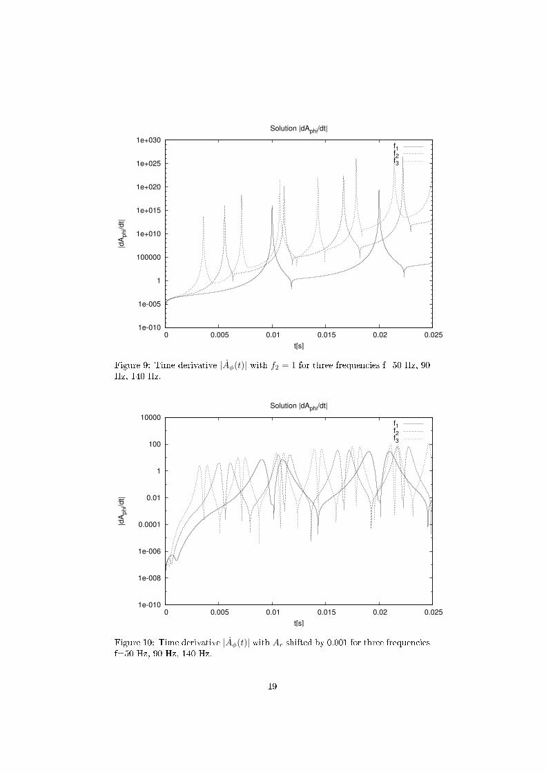
The structure is very similar to that of Aϕ itself.Next we have tested the dependence of the solution on the driving force f2.

It results that Aϕ is practically insensitive to the form of f2, provided the valueis di�erent from zero where ω0 has its poles. It is even su�cient to take a spikepulse of one percent of the time period. Fig. 9 shows the result for a constantvalue of f2.

Since the zero crossing of Ar is essential for the resonances, we have modi�edEq. (85) by adding a constant value of 0.001, thus displacing the curve of Fig.3 by this value from zero. The result (Fig. 10) shows a far smaller resonancestructure indicating that resonances are very sensitive to the form of Ar via ω0.

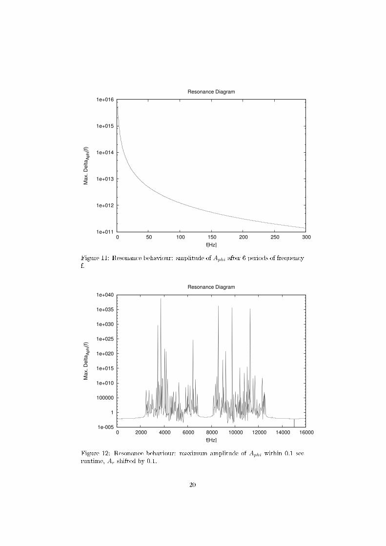
Next we inspect the development of the maximum amplitude. In Fig. 11 themaximum di�erence over the �rst six time periods is plotted in dependence of thetime frequency. Obviously the resonance is most dramatic for low frequencies.

15

0

0.2

0.4

0.6

0.8

1

0 0.005 0.01 0.015 0.02 0.025

Ar(

t)

t[s]

Input Model Ar(t)

f1f2f3

Figure 3: Radial component of vector potential Ar for three frequencies f=50Hz, 90 Hz, 140 Hz.

-1500

-1000

-500

0

500

1000

1500

0 0.005 0.01 0.015 0.02 0.025

dA

r/dt

t[s]

Input Model dAr/dt

f1f2f3

Figure 4: Time derivative Ar for three frequencies f=50 Hz, 90 Hz, 140 Hz.

16

1

100

10000

1e+006

1e+008

1e+010

1e+012

0 0.005 0.01 0.015 0.02 0.025

|om

ega

0|

t[s]

Input Model |omega0|

f1f2f3

Figure 5: |ω0| for three frequencies f=50 Hz, 90 Hz, 140 Hz.

100000

1e+006

1e+007

1e+008

1e+009

1e+010

1e+011

1e+012

1e+013

1e+014

1e+015

0 0.005 0.01 0.015 0.02 0.025

|d o

mega

0/d

t|

t[s]

Input Model |d omega0/dt|

f1f2f3

Figure 6: Time derivative |ω0| for three frequencies f=50 Hz, 90 Hz, 140 Hz.

17

1e-030

1e-020

1e-010

1

1e+010

1e+020

1e+030

0 0.005 0.01 0.015 0.02 0.025

|Ap

hi|

t[s]

Solution |Aphi|

f1f2f3

Figure 7: Solution |Aφ(t)| for three frequencies f=50 Hz, 90 Hz, 140 Hz.

1e-030

1e-020

1e-010

1

1e+010

1e+020

1e+030

1e+040

0 0.005 0.01 0.015 0.02 0.025

|dA

ph

i/dt|

t[s]

Solution |dAphi/dt|

f1f2f3

Figure 8: Time derivative |Aφ(t)| for three frequencies f=50 Hz, 90 Hz, 140 Hz.

18

1e-010

1e-005

1

100000

1e+010

1e+015

1e+020

1e+025

1e+030

0 0.005 0.01 0.015 0.02 0.025

|dA

ph

i/dt|

t[s]

Solution |dAphi/dt|

f1f2f3

Figure 9: Time derivative |Aφ(t)| with f2 = 1 for three frequencies f=50 Hz, 90Hz, 140 Hz.

1e-010

1e-008

1e-006

0.0001

0.01

1

100

10000

0 0.005 0.01 0.015 0.02 0.025

|dA

ph

i/dt|

t[s]

Solution |dAphi/dt|

f1f2f3

Figure 10: Time derivative |Aφ(t)| with Ar shifted by 0.001 for three frequenciesf=50 Hz, 90 Hz, 140 Hz.

19

1e+011

1e+012

1e+013

1e+014

1e+015

1e+016

0 50 100 150 200 250 300

Max. D

elta

Ap

hi(f)

f[Hz]

Resonance Diagram

Figure 11: Resonance behaviour: amplitude of Aphi after 6 periods of frequencyf.

1e-005

1

100000

1e+010

1e+015

1e+020

1e+025

1e+030

1e+035

1e+040

0 2000 4000 6000 8000 10000 12000 14000 16000

Max. D

elta

Ap

hi(f)

f[Hz]

Resonance Diagram

Figure 12: Resonance behaviour: maximum amplitude of Aphi within 0.1 secruntime, Ar shifted by 0.1.

20

1e-060

1e-040

1e-020

1

1e+020

1e+040

0 0.005 0.01 0.015 0.02 0.025

Inte

gra

l A

ph

i2/o

mega

t[s]

Radiated Energy

f1f2f3

Figure 13: Integral over radiated energy for three frequencies f=50 Hz, 90 Hz,140 Hz.

In the next �gure (Fig. 12) the maximum amplitude di�erence was recorded overa constant simulated time of 0.1 sec. To avoid numerical instabilities inferredby the calculation we used a modi�ed Ar input value as discussed for Fig.10 (shifted by 0.1 upwards, no zero crossing). Solutions are stable in the lowfrequency range but there are windows of unstability for higher frequencies. Weargue that the di�erential equation (78) can show chaotic behaviour and mustbe carefully evaluated.

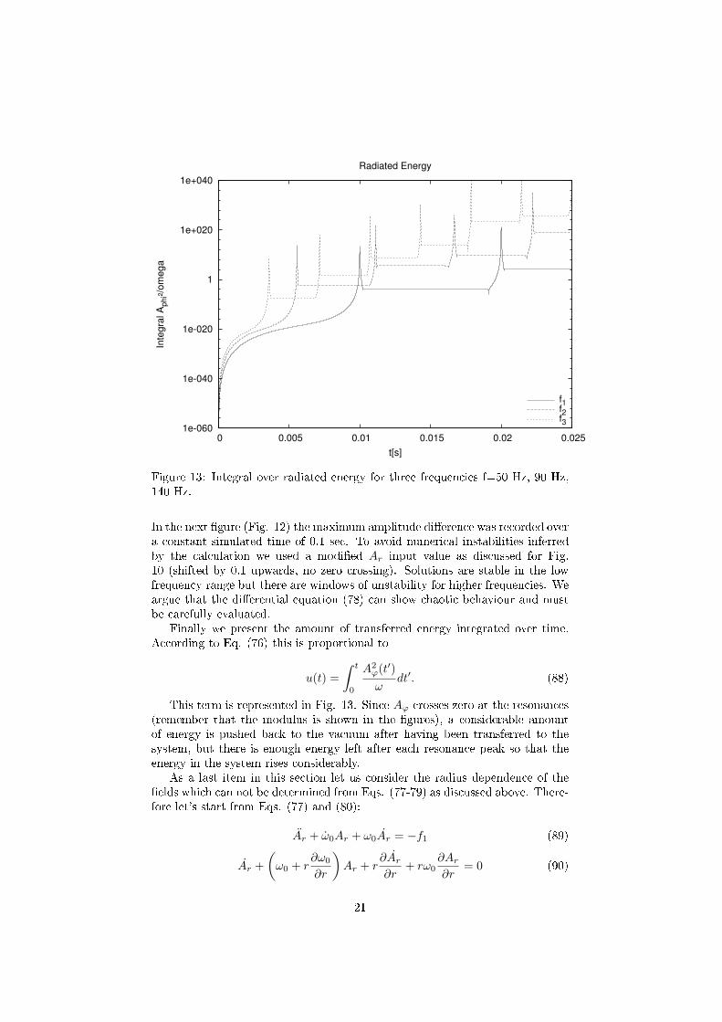
Finally we present the amount of transferred energy integrated over time.According to Eq. (76) this is proportional to

u(t) =∫ t

0

A2ϕ(t′)ω

dt′. (88)

This term is represented in Fig. 13. Since Aϕ crosses zero at the resonances(remember that the modulus is shown in the �gures), a considerable amountof energy is pushed back to the vacuum after having been transferred to thesystem, but there is enough energy left after each resonance peak so that theenergy in the system rises considerably.

As a last item in this section let us consider the radius dependence of the�elds which can not be determined from Eqs. (77-79) as discussed above. There-fore let's start from Eqs. (77) and (80):

Ar + ω0Ar + ω0Ar = −f1 (89)

Ar +(ω0 + r

∂ω0

∂r

)Ar + r

∂Ar∂r

+ rω0∂Ar∂r

= 0 (90)

21

We will make an ansatz for Ar and compute the solution for ω0 which iscompatible with this. We choose

Ar = C e−αr−iβt (91)

which is a conventional approach for a radially decreasing vector potentialwhich oscillates in time with frequency β. Inserting this into Eq. (89) resultsin a di�erential equation for ω0 in the variable t:

−(β2 + i ω0 β − ω0

)e−α r−i β C = −f1 (92)

The solution of this equation is

ω0(t) = c(r) eiβt + i β − f1t

Ceαr+i βt (93)

with a constant c(r) which is dependent on r in general. Inserting (93) into(90) yields

(i α β r − ω0 α r + ω0 r − i β + ω0) e−α r−i β t C = 0 (94)

which has the solution

ω0(r) =c(t)r

eα r + i β. (95)

Since both solutions (93) and (95) must be compatible, we have to assume

c(r) = 0. (96)

By comparison of both equations for ω0 (93 and 95) we �nd

c(t) = −f1 tCeiβ t (97)

and �nally

ω0(r) = −f1 tCeα r+iβ t + iβ. (98)

We see that the spin connection has a diverging behaviour in space as wellas in time which is consistent with the results of the numerical model.

4.6 Summary and discussion

The Bedini device has been analysed by analytical and numerical methods.Based on a model of cylindrical symmetry of the transducer, which is consideredto be the essential part for spacetime coupling, the following mechanism ofspacetime interaction could be identi�ed:

Under undisturbed conditions, the magnetic �eld in the transducer is cylin-drically symmetric. The radial part of the vector potential must vanish due tothe Gauss law. The passing magnets of the wheel distort the symmetry of themagnetic �eld in the transducer by inducing an asymmetric signal. This leadsto a radial component of the vector potential which was not present before.The vector potential changes in time and therefore induces an electric �eld.Consequently, the Coulomb law has to be ful�lled as an additional condition,

22

in this case for a vanishing charge density (the electric �eld is completely aradiated �eld). The ECE �eld equations show that for the Coulomb law theradial component of the vector potential has either to be zero, or the scalar spinconnection must exist to compensate a non-vanishing radial component of thevector potential. The latter case is ful�lled in the Bedini device and leads tothe observed resonant behaviour.

A model has been developed which takes a timely varying radial vectorpotential Ar as a given input. By means of the Coulomb law, a spin connectionω0 is produced. The zero crossings of Ar lead to a singular value of the spinconnection, leading in turn to very high values of the ϕ component of the vectorpotential. These are the giant resonances which are strong enough in practiceto transfer signi�cant amounts of energy from spacetime to the machine.

For some spacetime resonance experiments it is reported that there is a glow-ing or �uorescent light e�ect around the apparatus when it is at resonance. Atthe same time the measured current of the driving mechanism takes a minimum.This can qualitatively be explained by analyzing the contributions of the ECEelectric charge current density. It is given in general by

J = (R ∧A− ω ∧ F ) (99)

(in short hand notation) for the Hodge duals of curvature R and the elec-tromagnetic �eld F as well as the potential A. At spin connection resonance,it may happen that the term ω ∧ F outweights the curvature term. Then thecharge current can become signi�cantly smaller while the region of space hasa high energy density due to the large spin connection term. Obviously no�negative energy� is required to explain the e�ect.

The only experimental feature which cannot be directly related to our modelis the required behaviour of the driving current. According to Bedini, the motorpulse acts as driving force for the spacetime resonance and must be very shortand sharp without oscillations. The model calculations showed that the formof the driving force is not important as long as it is di�erent from zero at thediverging time positions of the spin connection.

Based on the results of this paper we can give some recommendations forfurther investigations and improvements of the Bedini design, under the prereq-uisite that our model is correct:

1. The vector potential Ar has to be provided in a way to have zero crossings.This could be enforced by positioning magnets with alternating polarityon the wheel.

2. Since mechanical parts limit the lifetime of a device, a design withoutmoving parts is desirable. The principles of the design can be retained byreplacing the wheel by a rotating electromagnetic �eld (for example basedon a three-phase AC voltage). Then arbitrary rotation frequencies can beapplied without mechanical restrictions.

3. E�ects of the asymmetry of the signal inducing the resonance should beinvestigated. For example it could be tested if a linear motion of a magnetperpendicular to the transducer would evoke resonance e�ects too.

23

Appendix 1: Reduction of form notation to vector

notation

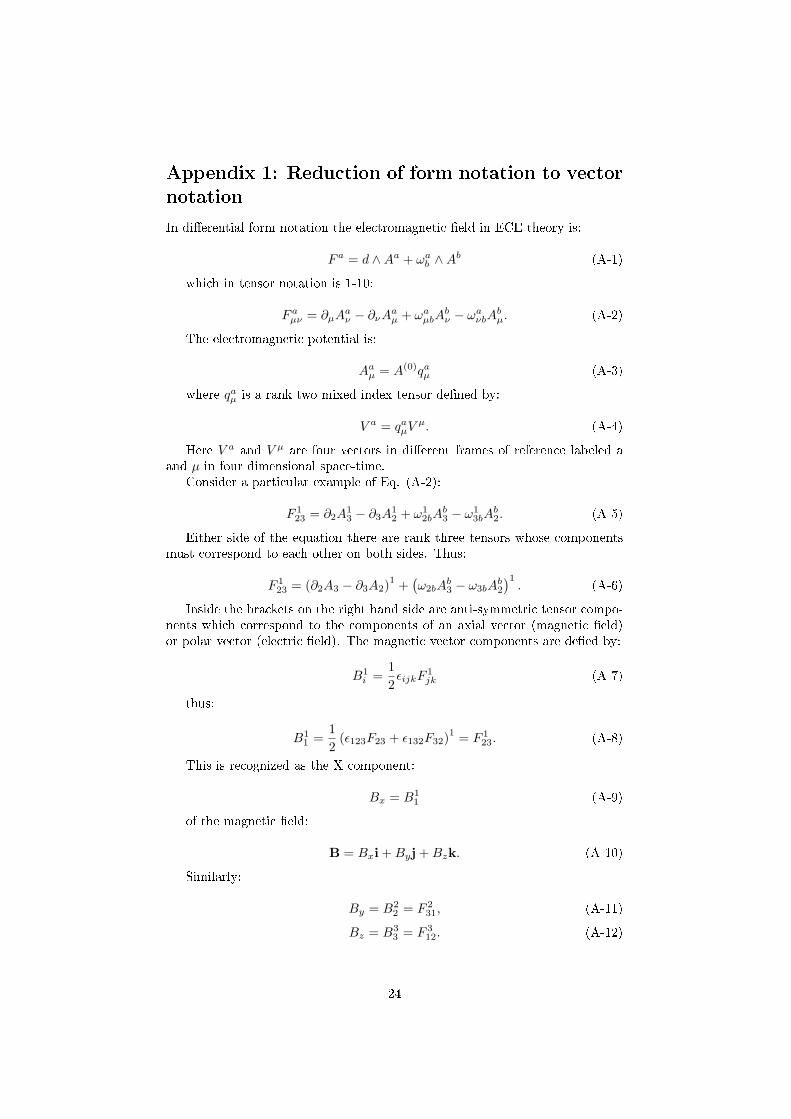
In di�erential form notation the electromagnetic �eld in ECE theory is:

F a = d ∧Aa + ωab ∧Ab (A-1)

which in tensor notation is 1-10:

F aµν = ∂µAaν − ∂νAaµ + ωaµbA

bν − ωaνbAbµ. (A-2)

The electromagnetic potential is:

Aaµ = A(0)qaµ (A-3)

where qaµ is a rank two mixed index tensor de�ned by:

V a = qaµVµ. (A-4)

Here V a and V µ are four vectors in di�erent frames of reference labeled aand µ in four dimensional space-time.

Consider a particular example of Eq. (A-2):

F 123 = ∂2A

13 − ∂3A

12 + ω1

2bAb3 − ω1

3bAb2. (A-5)

Either side of the equation there are rank three tensors whose componentsmust correspond to each other on both sides. Thus:

F 123 = (∂2A3 − ∂3A2)1 +

(ω2bA

b3 − ω3bA

b2

)1. (A-6)

Inside the brackets on the right hand side are anti-symmetric tensor compo-nents which correspond to the components of an axial vector (magnetic �eld)or polar vector (electric �eld). The magnetic vector components are de�ed by:

B1i =

12εijkF

1jk (A-7)

thus:

B11 =

12

(ε123F23 + ε132F32)1 = F 123. (A-8)

This is recognized as the X component:

Bx = B11 (A-9)

of the magnetic �eld:

B = Bxi +Byj +Bzk. (A-10)

Similarly:

By = B22 = F 2

31, (A-11)

Bz = B33 = F 3

12. (A-12)

24

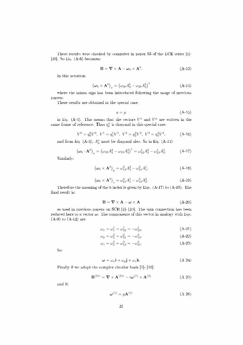
These results were checked by computer in paper 93 of the ECE series [1]-[10]. So Eq. (A-6) becomes:

B = ∇×A− ωb ×Ab. (A-13)

In this notation: (ωb ×Ab

)x

=(ω3bA

b2 − ω2bA

b3

)1(A-14)

where the minus sign has been introduced following the usage of previouspapers.

These results are obtained in the special case:

a = µ (A-15)

in Eq. (A-4). This means that the vectors V a and V µ are written in thesame frame of reference. Thus qaµ is diagonal in this special case:

V 0 = q00V0, V 1 = q11V

1, V 2 = q22V2, V 3 = q33V

3, (A-16)

and from Eq. (A-3), Aaµ must be diagonal also. So in Eq. (A-14)(ωb ·Ab

)x

=(ω32A

22 − ω23A

33

)1= ω1

32A22 − ω1

23A33. (A-17)

Similarly: (ωb ×Ab

)y

= ω213A

33 − ω2

31A11, (A-18)

(ωb ×Ab

)z

= ω321A

11 − ω3

12A22. (A-19)

Therefore the meaning of the b index is given by Eqs. (A-17) to (A-19). The�nal result is:

B = ∇×A− ω ×A (A-20)

as used in previous papers on SCR [1]- [10]. The spin connection has beenreduced here to a vector ω. The components of this vector in analogy with Eqs.(A-9) to (A-12) are:

ωx = ω11 = ω1

32 = −ω123, (A-21)

ωy = ω22 = ω2

31 = −ω213, (A-22)

ωz = ω33 = ω3

12 = −ω321. (A-23)

So:

ω = ωxi + ωyj + ωzk. (A-24)

Finally if we adopt the complex circular basis [1]- [10]:

B(3)∗ = ∇×A(3)∗ − iω(1) ×A(2) (A-25)

and if:

ω(1) = gA(1) (A-26)

25

we obtain the B(3)∗ spin �eld:

B(3)∗ = −igA(1) ×A(2). (A-27)

26

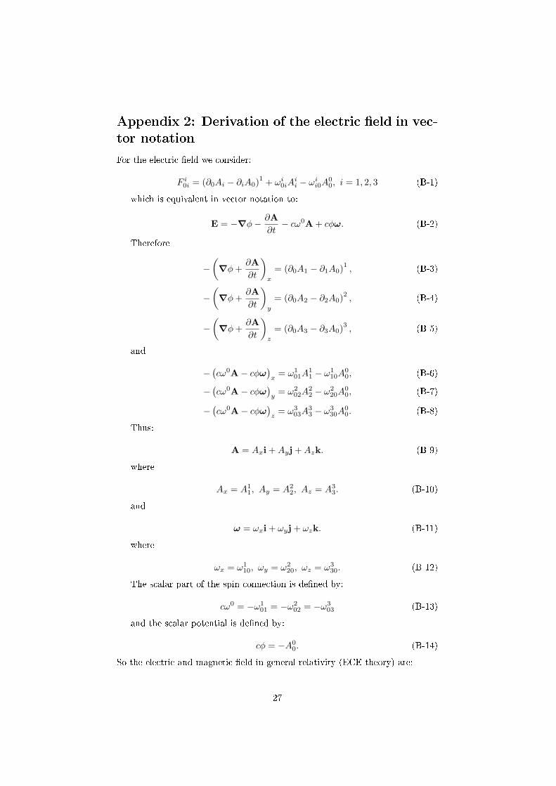
Appendix 2: Derivation of the electric �eld in vec-

tor notation

For the electric �eld we consider:

F i0i = (∂0Ai − ∂iA0)1 + ωi0iAii − ωii0A0

0, i = 1, 2, 3 (B-1)

which is equivalent in vector notation to:

E = −∇φ− ∂A∂t− cω0A + cφω. (B-2)

Therefore

−(

∇φ+∂A∂t

)x

= (∂0A1 − ∂1A0)1 , (B-3)

−(

∇φ+∂A∂t

)y

= (∂0A2 − ∂2A0)2 , (B-4)

−(

∇φ+∂A∂t

)z

= (∂0A3 − ∂3A0)3 , (B-5)

and

−(cω0A− cφω

)x

= ω101A

11 − ω1

10A00, (B-6)

−(cω0A− cφω

)y

= ω202A

22 − ω2

20A00, (B-7)

−(cω0A− cφω

)z

= ω303A

33 − ω3

30A00. (B-8)

Thus:

A = Axi +Ayj +Azk. (B-9)

where

Ax = A11, Ay = A2

2, Az = A33. (B-10)

and

ω = ωxi + ωyj + ωzk. (B-11)

where

ωx = ω110, ωy = ω2

20, ωz = ω330. (B-12)

The scalar part of the spin connection is de�ned by:

cω0 = −ω101 = −ω2

02 = −ω303 (B-13)

and the scalar potential is de�ned by:

cφ = −A00. (B-14)

So the electric and magnetic �eld in general relativity (ECE theory) are:

27

E = −∇φ− ∂A∂t− cω0A + cωφ. (B-15)

B = ∇×A− ω ×A. (B-16)

28

References

[1] M. W. Evans, "Generally Covariant Uni�ed Field Theory" (Abramis, Suf-folk, 2005 onwards), volumes one to four, volume �ve in prep. (Papers 71to 93 on www.aias.us).

[2] L. Felker. "The Evans Equations of Uni�ed Field Theory" (Abramis, Suf-folk, 2007).

[3] K. Pendergast, "Crystal Spheres" (Abramis to be published, preprint onwww.aias.us, 2008).

[4] M. W. Evans, Acta Phys. Polonica, 38, 2211 (2007).

[5] M. W. Evans and H. Eckardt, Physica B, 400, 175 (2007).

[6] M. W. Evans, Physica B, 403, 517 (2008).

[7] M. W. Evans, Omnia Opera of www.aias.us, 1992 to present.

[8] M. W. Evans and H. Eckardt, Paper 63 of www.aias.us, published in volumefour of ref. (1).

[9] M. W. Evans, reviews in Adv. Chem. Phys., vols. 119(2) and 119(3) (2001).

[10] M. W. Evans and L. B. Crowell, "Classical and Quantum Electrodynamicsand the B(3) Field" (World Scienti�c, 2001); M. W. Evans and J.-P. Vigier,"The Enigmatic Photon" (Kluwer, Dordrect, 1994 to 2002, hardback andsoftback), in �ve volumes.

[11] J. Bedini, US patents on the Bedini devices: US Patent No.6,392,370 (2002), 6,545,444 (2003), 20020097013 (2002), 20020130633(2002); industry certi�cation test report (German TUV, 2002) underhttp://www.icehouse.net/john34/bedinibearden.html.

[12] E. G. Milewski, ed., "Vector Analysis Problem Solver" (Education Associ-ation, New York, 1984).

[13] J. Bedini and T. E. Bearden, �Free Energy Generation�, Cheniere Press,2006.

[14] http://tech.groups.yahoo.com/group/Bedini_Monopole.

29