Split Incentives in Residential Energy Consumption

Kenneth Gillingham, Matthew Harding, and David Rapson

August 17, 2011

Kenneth GillinghamYale University

School of Forestry & Environmental Studies195 Prospect Street

New Haven, CT 06511Phone: (650) 353-6578

Email: kenneth.gillingham@yale.edu

Matthew HardingStanford University

Department of Economics579 Serra Mall

Stanford, CA 94305Phone: (650) 723-4116

Fax: (650) 725-5702Email: mch@stanford.edu

David RapsonUniversity of California, Davis

Department of EconomicsOne Shields AveDavis, CA 95616

Phone: (530) 752-5368Email: dsrapson@ucdavis.edu

Split Incentives in Residential Energy Consumption

We explore two split incentive issues between owners and occupants of residential dwellings: heat-

ing or cooling incentives are suboptimal when the occupant does not pay for energy use, and insu-

lation incentives are suboptimal when the occupant cannot perfectly observe the owner’s insulation

choice. We empirically quantify the effect of these two market failures and how they affect behav-

ior in California. We find that those who pay are 16 percent more likely to change the heating

setting at night and owner-occupied dwellings are 20 percent more likely to be insulated in the at-

tic or ceiling. However, in contrast to common conception, we find that only small overall energy

savings may be possible from policy interventions aimed at correcting the split incentive issues.

JEL: Q4,Q5

Keywords: principal-agent; asymmetric information; CO2 emissions.

1

1. INTRODUCTION

It is often claimed that differing incentives between owners and occupants of residential dwellings

lead to the over-consumption of energy. For example, the New York Times recently quoted build-

ing managers in New York estimating that apartments that do not pay for electricity “expend at

least 30 percent more electricity year-round than their counterparts” and suggested that this came

with a “considerable environmental cost” (New York Times 2010). The concern here is that apart-

ment occupants face a zero marginal cost for the energy used to provide cooling. An identical split

incentive issue may occur when occupants do not pay for heat. Differing incentives may also occur

when a prospective occupant imperfectly observes the owner’s choice of energy efficiency of the

dwelling, reducing the owner’s incentive to properly insulate the dwelling. These issues of differ-

ing incentives are principal-agent problems that have the potential to lead to inefficient allocation

of resources. In the policy realm, these potential market failures are often used to justify energy

efficiency standards or other regulatory actions. With residential buildings making up just over 20

percent of 2006 primary energy demand in the United States, and with over a third of all occupied

housing units being rental units, the amount of energy consumption affected by these misaligned

incentives might reasonably be expected to be substantial (EIA 2008, US Census Bureau 2010).

Yet, to date, our understanding of these split incentive issues in residential energy consumption is

remarkably limited.

We provide empirical evidence quantifying the magnitude of split incentives issues in California.

First, we find evidence of a heating or cooling split incentive issue when the occupant does not pay

for heating or cooling. For example, households that pay for heating are 16 percent more likely

to change the heating setting at night. Second, we find evidence of an insulation split incentive

issue due to asymmetric information in the contracting process between the owner and prospective

2

occupant. We find that owner-occupied dwellings where the resident pays for heating and cooling

are 20 percent more likely to be insulated in the attic or ceiling and 13 percent more likely to be

insulated in the exterior walls.

There is a long history of economic theory developed to explain a variety of situations where

two parties have differing incentives, usually occurring in settings where there is asymmetric in-

formation between a principal and an agent either before or after the contracting phase (e.g., Ar-

row (1963), Spence and Zeckhauser (1971), Alchian and Demsetz (1972), Jensen and Meckling

(1976), Grossman and Hart (1982), Laffont and Martimort (2001)). The possibility of split incen-

tives between owners and occupants of residential dwellings was first described with case stud-

ies indicating a “landlord-tenant” issue of asymmetric information leading to less insulation and

less energy efficient appliances than might otherwise be expected (Blumstein, Krieg, Schipper,

and York 1980). Since then, split incentives between owners and occupants have been quali-

tatively discussed in a variety of studies elucidating the potential market failures that may im-

pede investments in improving residential energy efficiency (Fisher and Rothkopf 1989, Jaffe

and Stavins 1994, Nadel 2002, Gillingham, Newell, and Palmer 2006, Gillingham, Newell, and

Palmer 2009).

Murtishaw and Sathaye (2006) provide quantitative estimates of the potential importance of

principal-agent problems between landlords and tenants in several areas of residential energy use.

Specifically, they examine the number of dwellings that may be affected by split incentive issues

in at least one type of energy use, and use this number to calculate a theoretical upper bound of

energy savings possible if policies could be implemented to entirely address these issues. They find

that 35 percent of residential energy use may be affected by at least one split incentive problem,

suggesting that the issue may be a large one. A report by the International Energy Agency (2007)

3

looks at case studies of situations where split incentives appear to be very important. Both of

these studies discuss the differing ways that split incentives may occur in energy consumption, but

neither provides empirical evidence of the extent to which the different types of problems may

exist.

Levinson and Niemann (2004) provide empirical evidence for a principal-agent problem when

landlords pay for heat. Levinson and Niemann use the US Department of Energy’s Residential En-

ergy Consumption Survey (RECS) to note that when heat is included in the rent, the average winter

indoor temperature is higher than when the heat is not included. Davis (2009) empirically exam-

ines the possibility of a principal-agent problem in the purchase of energy efficient appliances by

landlords when occupants pay the electricity bill. Davis finds that after controlling for household

covariates, landlords who do not pay the electricity bill are less likely to have purchased “Energy

Star” appliances.1

We find only limited empirical evidence for a split incentive issue in the level of temperature set-

ting for heating or cooling, and posit that these findings may be partly related to heterogeneity in

preferences for heat at different times of day. However, we find stronger evidence that split incen-

tives can affect behavior by influencing when occupants change their temperature setting. Those

who do not pay for heating or cooling are less likely to change the setting. We also find statisti-

cally significant evidence that owner-occupied dwellings where the owner pays for heat are more

likely to be insulated. Using these empirical results, we perform a back-of-the-envelope calcula-

tion, which indicates that while split incentive issues may change household behavior, the resulting

energy and carbon dioxide savings from fully correcting for these issues would be moderate, with

greater savings coming from the insulation split incentive issue. This result can be explained by

1To achieve the Energy Star designation from the U.S. Environmental Protection Agency, an appliance must meet astringent standard for energy efficiency.

4

the small number of households who do not pay for heat and the moderate behavioral changes we

find for both insulation and heating or cooling. An implication of these results is that while cer-

tain low-cost policies may improve economic efficiency by addressing market failures from split

incentive issues, addressing these issues would not dramatically change energy use or even be sig-

nificant step toward meeting California’s obligations under the Global Warming Solutions Act of

2006 (Assembly Bill 32).

This paper is structured as follows. In the next section, we provide a conceptual framework to

help formalize when and how split incentives in the owner-occupant relationship may lead to an

overconsumption of energy. This framework provides the hypotheses to be tested in our empirical

analysis. The third section describes our dataset. The fourth section quantifies each aspect of the

split incentive problem, reporting our empirical results for heating, cooling, and insulation. The

next section describes the results of our back-of-the-envelope calculations, quantifying a rough up-

per bound for the energy savings that policies to address these split incentive issues could achieve.

The final section concludes with a discussion of implications for energy efficiency policy.

2. CONCEPTUAL FRAMEWORK

Split incentives can occur when the dwelling is either owned or rented, depending on whether

the occupant pays the energy bill. This section presents a conceptual framework for the split

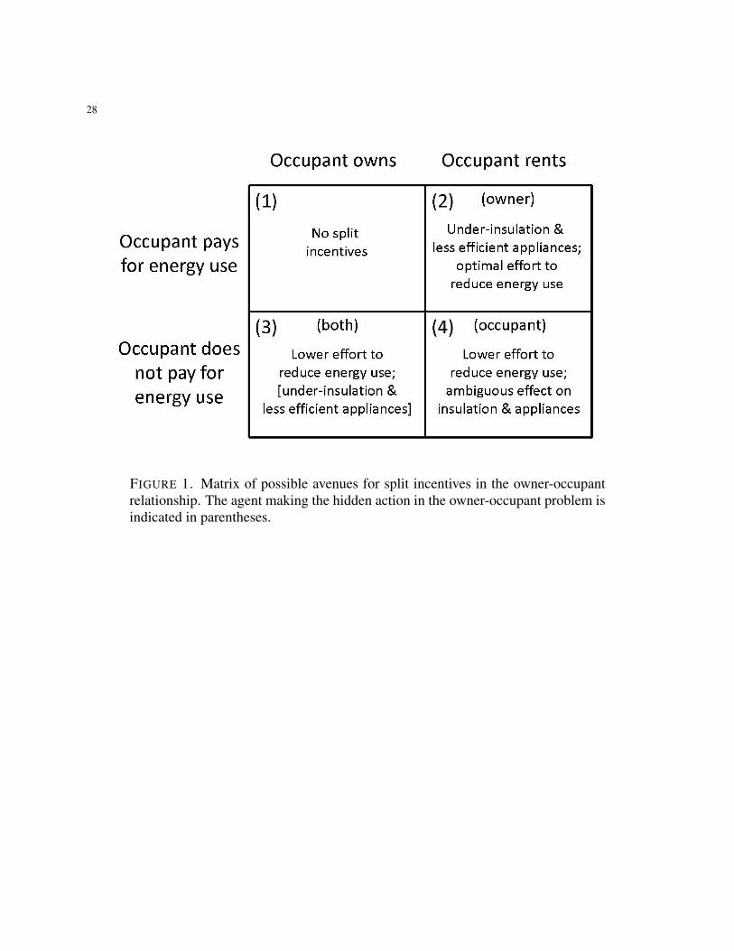
incentive issues we will investigate empirically in the later sections.2 Figure 1 indicates three

possible avenues for split incentives to play a role.

[ Figure 1 about here ]

2We also mathematically formalize this conceptual framework in a contract theory model of the principal-agent prob-lems. This model is available on the authors’ websites or upon request.

5

In the upper left box (1), the dwelling is owner-occupied and the occupant pays for energy use.

There are no split incentive concerns here.3 In the lower right (labeled (4)), the occupant is a renter

and does not pay for at least some part of their energy use, such as heating, central cooling, or even

electricity. In this case, the occupant faces a zero marginal cost for energy use and thus has little

incentive to pay attention to the amount of energy used, which can be thought of as a principal-

agent problem where the owner is a principal and tenant is an agent. This may lead to greater

use of heating or cooling, less effort exerted to change heating or cooling settings (e.g., turning

heating down at night), or fewer purchases of energy-efficient appliances.4 Since the owner is

paying for energy use and also making the choice of the level of insulation and energy efficiency

of appliances, the owner’s incentives to invest in efficiency are theoretically ambiguous. There are

two effects that work in opposite directions. If the owner expects the occupant to over-consume

energy, then the owner may over-invest in insulation to compensate. On the other hand, if the

owner is unable to fully capitalize investment in efficiency into the rent or property resale value,

the owner may choose to under-invest in efficiency.

The upper right box (2) shows a situation where the occupant is a renter who pays for all of his or

her energy use, but may not be able to perfectly observe previous choices made by the owner that

affect the energy efficiency of the dwelling. In this case, the owner has little incentive to insulate the

dwelling or to install energy-efficient appliances (e.g., refrigerators, washers & dryers). Here there

is a principal-agent problem where the owner is the agent who makes a (partly) hidden action.

Davis (2009) finds empirical evidence for this particular issue in the context of energy-efficient

appliances. Since the occupant pays for the energy use, the occupant has an incentive to pay

3This presumes that home improvements are fully capitalized – or at least that consumers consider this to be the case.4Levinson and Niemann (2004) provide empirical evidence for a greater use of heating in this particular situation, butdo no consider the insulation decision.

6

attention to the use of energy, and thus there is less likely to be a principal-agent problem relating

to the effort to reduce energy use from the existing stock of durable goods in the household.5

In the bottom left (box (3)), the dwelling is owner-occupied, but for some reason, the occupant

does not pay for at least some part of the energy use. This is most likely to occur for townhouses

and other attached housing complexes. Since the occupant does not pay for his or her entire

energy use, he or she may keep the heating set higher and cooling set lower, and may make fewer

purchases of energy-efficient appliances (as in box (4)). In addition, there may be a split incentive

issue where the third-party provider of the energy is the agent in the principal-agent problem, as

in box (2). This issue would only occur if the occupant is responsible for the choice of insulation

and the energy efficiency of the appliances but does not pay for the energy use. While this may

occur in some settings, often in attached housing complexes where the owner-occupiers do not

pay for their energy use, in most cases there are guidelines determining the amount of insulation

required. In addition, it is possible for the payer of the energy bill to install additional insulation or

energy-efficient appliances themselves. Thus, the split incentive issue may be internalized through

creative contracts. Hence, we include “under-insulation and less efficient appliances” in brackets

in Figure 1.

2.1. Testable implications. The framework developed above provides several testable implica-

tions for our empirical analysis:

• We expect occupants who rent their dwellings and pay for heating or cooling to reside in

under-insulated dwellings relative to those who rent and do not pay for heating or cooling

(box (2) in Figure 1).

5A principal-agent problem could still occur for energy-efficient investments by the occupant if the investment has alonger lifespan than the expected length of the lease.

7

• We expect occupants who do not pay for their heating or cooling to put in less effort to

reduce their heating and cooling use relative to those who pay for their heating or cooling

(boxes (3) and (4) in Figure 1). This can come about through changing heating or cool-

ing settings more often, higher temperatures when heating, and lower temperatures when

cooling. This is also expected regardless of whether the tenant owns or rents the dwelling.

• We expect occupants who own their dwelling and do not pay for their heating or cooling to

under-insulate their dwelling relative to those who own and pay for their heating or cooling

(box (3) in Figure 1).

3. DATA

3.1. Data sources. Our dataset is from the California Statewide Residential Appliance Saturation

Study (RASS), which was administered by the California Energy Commission. The study sur-

veys households in California to assess the determinants of the saturation of different appliances

in order to inform the utility planning process. The survey was performed in 2003, and involved

first sending out mail surveys to 100,000 single-metered homes randomly chosen throughout Cal-

ifornia. After two rounds of mail surveys, 18,970 responses were received. To address possible

participation bias, a sample of 2,183 of the non-respondents were contacted, either through a third

mail survey with an incentive, a telephone interview, or an in-person interview.6 In addition, there

was a separate process for master-metered customers. In a first stage, 616 telephone surveys were

conducted with the manager of the master-metered facility. Following this, mail surveys were sent

to the individual customers within each of the master-metered facilities, with a follow-up phone

interview to raise response rates. Of the 5,593 surveys sent out, 767 were completed and returned.

6The characteristics of the non-respondents do not appear to differ appreciably from those who first responded.

8

After combining these data, the end result is a dataset of 20,933 responses designed to be rep-

resentative of California households in terms of geography, income, housing type, and other key

characteristics.7

While the California Energy Commission took significant steps to ensure unbiased participation

across the different demographic groups, some participation issues could not be eliminated. Ex-

tremely low and extremely high users of electricity did not participate in the surveys. There also

appears to be some under-reporting by the hispanic population in part due to undocumented resi-

dents. The overall participation rate, while relatively low, is consistent with other recent California

surveys.

We augmented the RASS dataset with 2003 electricity price data from each electric utility. The

data were matched based on the annual kilowatt-hour (kWh) electricity consumption and utility

climate zone of the electricity customer. California has a “tiered-rate” electricity price schedule,

whereby consumers pay a low rate for consumption below a certain amount, a higher rate for the

next increment of consumption, and so on.8 The annual kWh consumption variable in the RASS

dataset allows us to place each observation on the electricity price tier they are most likely on – so

each household is matched with the most likely marginal price they face.

We recognize that this electricity price variable has limitations in an analysis of consumer behav-

ior, for there is some evidence that consumers do not realize what tier they are on, and thus what

marginal price of electricity they are being charged. For example, we cannot rule out that con-

sumers may make decisions based on the average price of electricity (Borenstein 2009, Ito 2010).

Moreover, RASS only contains the annual kWh electricity consumption, but consumers may be

7In cleaning the dataset, we dropped a small number of observations that were coded as living in mobile homes or“other” dwellings, or had more than 10 children.8See Borenstein (2008) and Borenstein (2009) for further details of California’s tiered electricity pricing schedule.

9

on different tiers at different months of the year. Finally, some electricity customers receive lower

rates if they are low income customers or have medical conditions and we do not observe these

particular situations. Fortunately, we find our results are completely insensitive to the inclusion or

exclusion of the electricity price variable.

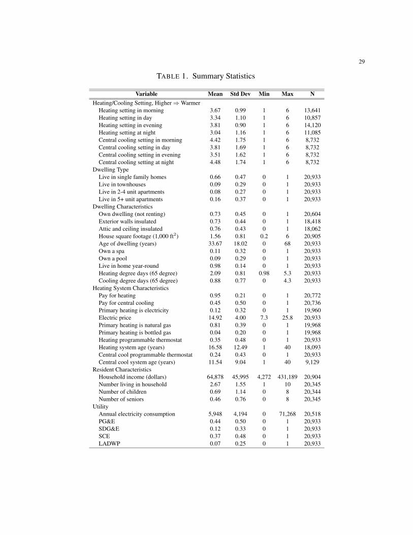
3.2. Summary statistics. The key variables from the RASS dataset used in this study include

a variety of housing characteristics, demographics, and, most importantly, owner and occupant

choices that may be affected by principal-agent problems. Summary statistics for these variables

in our full final cleaned dataset are given in Table 1.

[ Table 1 about here ]

The reported heating and cooling settings at different times of day (i.e., morning, day, evening,

and night) are two of our primary variables of interest that help us identify a heating or cooling

split incentive issue. These take values from one to six. For the heating variables, these correspond

having heat below 55◦F, 56− 60◦F, 61− 65◦F, 66− 70◦F, 71− 75◦F, and over 75◦F. For the central

cooling variables, these categories correspond to having the temperature below 70◦F, 70 − 73◦F,

74− 76◦F, 77− 80◦F, and over 80◦F.

The RASS dataset also includes two variables capturing the degree to which the dwelling is

insulated. One variable of interest is an indicator variable for whether the attic/ceiling of the

dwelling is insulated at all. The second variable of interest is an indicator variable for whether at

least some of the exterior walls of the dwelling are insulated.9

We take a separate subsample of our final cleaned dataset for our heating and cooling results.

Specifically, we recognize that heating costs are not likely to be a major concern for large areas

9This variable is created from a categorical variable taking a value one for “yes, all”, two for “yes, some”, and threefor “no.” An alternative coding of one if “yes, all” and zero otherwise gives similar results.

10

of Southern California that rarely use much heating, so we take a subsample where we include

all observations with greater than 2,000 65◦F heating degree days (HDD65), where HDD65 are

defined as the difference between the average temperature in that day and 65◦F summed over all

days of the year that are cooler than 65◦F.10 By focusing on consumers in cooler climates, we can

examine behavioral responses from those consumers for whom we would expect heating bills to be

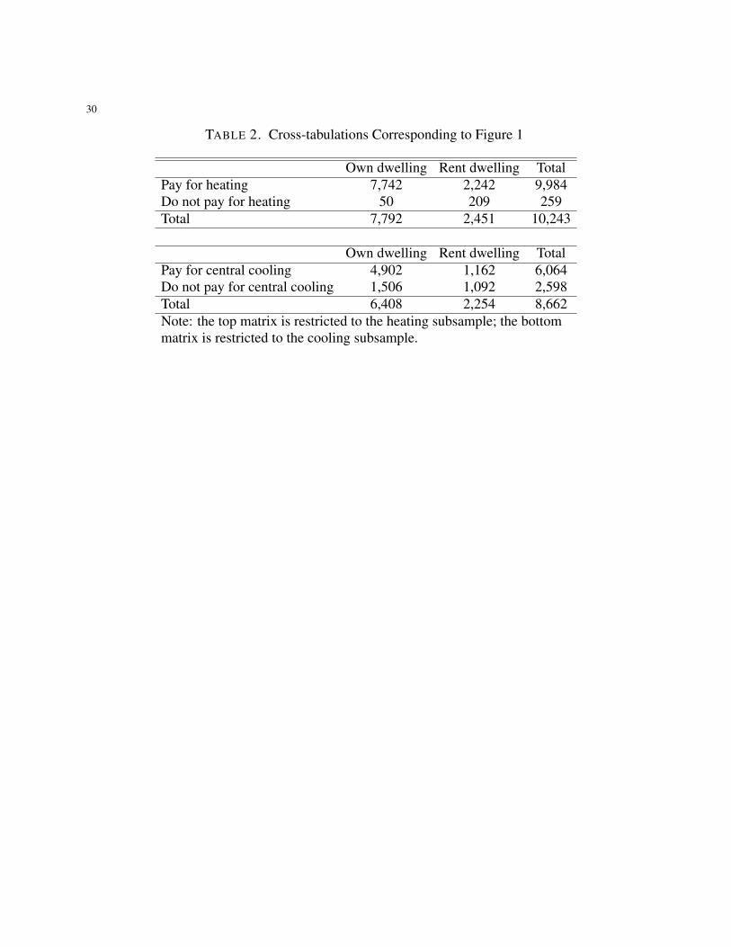
significant. This heating subsample consists of 10,453 observations. For this subsample, Table 2

(top) gives a cross-tabulation for the number of observations that fall into the categories described

in Figure 1. This cross-tabulation indicates that much of the sampled population (76 percent) falls

into box (1) in Figure 1, where there are no split incentive issues. The cross-tabulation also shows

that a reasonable number of the observations fall within categories where there are split incentive

issues, and in particular box (2), where we would expect to find under-insulation (22 percent).

[ Table 2 about here ]

Similarly, cooling costs are not likely to be a major concern for much of Northern California.

Thus, we take a subsample in which we include all observations with greater than 1,000 65◦F

cooling degree days (CDD65), where CDD65 are defined as the difference between the average

temperature in that day and 65◦F summed over all days of the year that are warmer than 65◦F.

We consider this subsample much more likely to capture the behavioral responses from those

consumers for whom we would expect cooling bills to be significant. This cooling subsample

consists of 8,800 observations. The bottom half of Table 2 gives a cross-tabulation for the number

of observations that use central cooling and fall into the categories described in Figure 1. We focus

on central cooling, rather than room air conditioning, due to the data availability for central cooling

and the greater ability to control the temperature in centrally cooled dwellings. Just as for heating,10The choice of 2,000 HDD65 is somewhat arbitrary, but the results do not appear to change appreciably with reason-able changes to this assumption.

11

the cross-tabulation shows that much of the sampled population (57 percent) is not subject to split

incentive issues, for it falls into box (1) in Figure 1. However, over 30 percent do not pay for

cooling, and thus may have split incentives leading to less effort to reduce cooling use (boxes (3)

and (4)). Since insulation is an important factor for energy use in both hot and cold climates, we

use the combined sample when analyzing the insulation choice.

4. ESTIMATION OF HOUSEHOLD BEHAVIOR

The conceptual framework in Section 2 suggested several hypotheses that can be tested in our

data. We begin by discussing the estimation of whether homeowners invest effort in order to save

energy, the split incentive issue indicated in boxes (3) and (4) in Figure 1. An attractive feature

of our dataset for this purpose is that we observe the heating and cooling settings in the home at

different times of the day. As discussed in the previous section, the temperature settings are defined

as ordered choices that fall into six distinct bins corresponding to the temperature interval.11

To begin, we ask: are households that do not pay for heat more likely to have a higher heating

setting? Consider a model for heating choices,Hj,t = {1, 2, 3, 4, 5, 6} for household j in period t =

{morning, day, evening, night}. Let H∗j,t be a continuous latent variable denoting the optimal

setting:

(1) H∗j,t = αt + βtPayj + γtOwnj +

∑c

δt,cCj,c +∑d

ηt,dDj,d + uj,t.

We thus model the optimal temperature setting decision as a function of whether the household

pays for heating (Payj) or owns the dwelling (Ownj), as well as a variety of dwelling characteris-

tics (C). The most important dwelling characteristics are the quantity of insulation, the price and

11It is tempting to model this variable as interval-coded data, but we are concerned that the surveyed households mayhave interpreted the categories loosely when filling out the survey – thus interpreting the variable as a series of orderedchoices appears more reasonable.

12

type of heating, the heating degree days, the geographic location of the home, the size of the living

space, and the availability of a programmable thermostat. Additionally, we model the decision as

also depending on household characteristics (D) such as income, number of children and elderly

residents, and education levels. The error term uj,t is assumed to be Normally distributed.

Furthermore, let us assume that there is a sequence of cut-off points τ0, τ1, τ2, . . . such that

intervals on H∗j,t map into the reported approximations of heating settings throughout the day in a

monotonic fashion. Thus, for example, a report of Hj,t = 2, or “56 − 60◦F,” corresponds to the

latent heating choice greater than τ0 but less than τ1. The cut-off points are known to the household

but not observed by the econometrician. Under the Normality assumption on the error distribution,

the probability of observing a report of “56− 60◦F” for household j in period t corresponds to the

probability:

(2) Pr(τ0 < H∗j,t < τ1) = Φ(τ1 − νj,t)− Φ(τ0 − νj,t),

where νj,t = αt + βtPayj + γtOwnj +∑

c δt,cCj,c +∑

d ηt,dDj,d, and Φ(·) denotes the standard

Normal cdf. The unknown parameters of the model (including the cut-off points) can thus be

estimated by maximum likelihood as an ordered probit model. For ease of interpretation, we are

interested in the estimated marginal effects evaluated at the mean.

The marginal effect of a change in some dwelling attribute Cc on a given heating setting s is

given by:

(3)∂Pr(Ht = s)

∂Cc

= δt,c(φ(τs − ν̄t)− φ(τs−1 − ν̄t)),

which we evaluate at the mean values of the covariates ν̄t, and φ(·) denotes the standard Normal

pdf. The marginal effect with respect to all of the other covariates are defined similarly. An

analogous specification can be assumed for central cooling.

13

While this empirical model is easy to estimate and represents a convenient reduced form spec-

ification for the choice of a heating setting, the parameters of interest are only identified with our

cross-sectional data if we believe that our controls entirely capture household-level heterogeneity

that may be correlated with whether or not the household pays for heating. Our rich set of covariate

controls may well be sufficient. However, all but a small percentage of households pay for their

heating (three percent of the heating subsample), so a relatively small number of households will

be identifying the coefficients in each of the heating setting bins.

These factors suggest that in addition to examining the level of the temperature setting, it may

also be worthwhile to examine other features of the data that also imply a split incentive issue.

Section 2 suggests that rational individuals who pay for their heat would change their temperature

settings during the day to reduce energy use during times of lower heating needs. For example, a

household looking to save energy may consider reducing or switching off the heating during the

day when they are at work, even if they have a strong preference for warmth when they are at home.

The ordered temperature settings in the RASS dataset are well-suited to this type of analysis. In

this case, we only must believe that households choose a living arrangement (i.e., whether to live

in a place where heat is paid for) based on larger factors and not on the effort cost of changing the

thermostat. This appears very plausible.

We define an indicator variable Yj which equals 1 if the household changes the heating settings

during the day, thereby exhibiting effort to reduce energy use. We then posit the following probit

model:

(4) Pr(Yj = 1) = Φ

(α + βPayj + γOwnj +

∑c

δcCj,c +∑d

ηdDj,d

).

14

We assume that the above equation corresponds to the reduced form of the optimal decision of

whether to change the heating setting. We report the estimated marginal effects ∂Pr(Y=1)∂Cc

= δcφ(ν̄),

where ν̄ corresponds to α+βPayj+γOwnj+∑

c δcCj,c+∑

d ηdDj,d evaluated at the mean values.

Of course, whether or not a household changes the heating settings at all during the day is just

one of several plausible empirical models of heating setting switching behavior. We also examine

analogous models where the dependent variable equals one if the household changes the heating

setting between morning and evening, evening and night or night and morning. Furthermore, we

explore whether households set their heating warmer in the evening than at night and warmer in

the morning than at night. We also examine a analogous specifications for central cooling to all of

those described above.

Finally, we can examine the insulation split incentive issue using a similar probit model to (4).

The dependent variable for the insulation regression is either an indicator variable for whether

the walls are insulated or an indicator variable for whether the attic/ceiling is insulated. In these

estimations we can explore the relationship between the presence of insulation and whether the

home is owner-occupied, while controlling for a number of home characteristics and resident de-

mographics. Throughout we report estimated marginal effects evaluated at the mean.

5. EMPIRICAL RESULTS

5.1. Heating and cooling.

5.1.1. Heating and cooling settings. First let us investigate how the probability that a consumer

is in any one of the heating or cooling setting bins changes if the consumer pays for their energy

use. We would expect to find that households who pay for their energy use will attempt to save on

15

their energy bill by lowering the level of heating in their home. Surprisingly, we find only limited

support for this hypothesis.

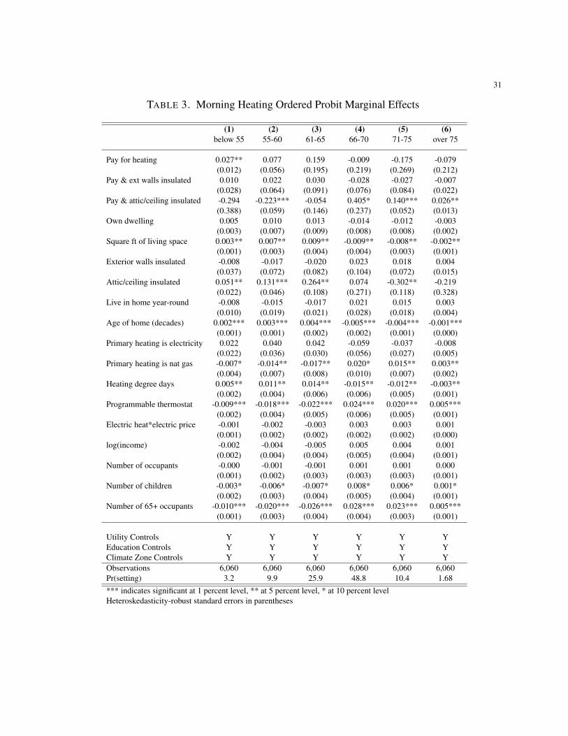
[ Table 3 about here ]

Tables 3 presents marginal effects estimated from the ordered probit model for heating settings in

the morning. The columns of the tables correspond to the different heating bins. One can interpret

the results as changes in the probability of choosing a given temperature setting in response to a

change in the covariates for the mean household. We find extremely similar results for other times

of day, although with more significance in other bins and less in the below 55◦F bin. However, the

signs and the general magnitude of the coefficients are similar. The central cooling results are also

similar but with slightly less statistical significance.

These findings suggest that households who pay for heat are more likely to select lower heating

settings below 65◦F. The results for the other categories display the sign we would expect, but are

for the most part not statistically significant. One possible explanation for not finding a stronger

relationship is that the energy bill is just not very salient in consumer decision-making. We view

this as possible, but less likely given the statistically significant results in Levinson and Niemann

(2004). Alternatively, these results can be viewed as attesting to the importance of heterogene-

ity in preferences over heating levels, a possible endogeneity concern that we cannot control or

instrument for. This provides motivation for the changes specification in the next section.

Several of the other coefficients point to the most important factors determining the heating

setting – many of which appear to dominate paying for heat in importance. We find statistically

significant evidence that households with larger houses or who live in colder climates choose lower

heating settings both in the morning and at night. We interpret this as reflecting the difficulty of

heating such homes to a higher degree, which may present both technological challenges as well as

16

substantially higher costs. Similarly, we find that homes with more children and seniors are heated

to a higher degree, reflecting the increased level of heating required for comfort in such homes.

5.1.2. Changes in heating and cooling settings. Our second estimation strategy focuses on whether

households make changes to their heating or cooling settings during the day in response to eco-

nomic incentives. This estimation strategy is less likely to suffer from unobserved heterogeneity

since irrespective of the chosen level of heating it remains rational to make changes between differ-

ent periods during the day. For example, one can save energy by turning down the heating during

the day or at night.

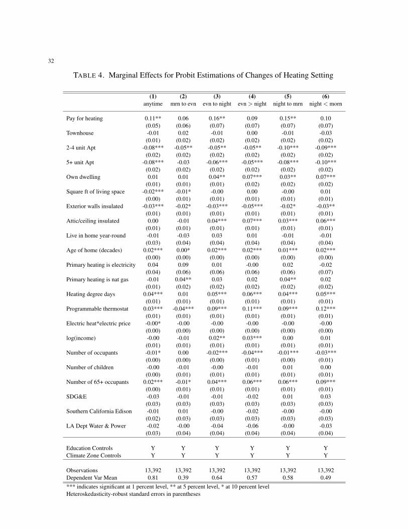
Table 4 reports the estimated marginal effects. The columns of this table correspond to different

dependent variables. Column 1 reports the results of a model where the dependent variable is

an indicator for whether the household made any changes to the heating setting during the day.

Columns 2, 3, and 5 analyze the cases where households choose different settings in the morning

and evening, evening and night and night and morning respectively. Column 4 reports the results

of a probit model where households choose a higher setting in the evening than at night, as would

be expected. Column 6 reports the corresponding results when a household chooses a lower setting

at night than in the morning.

[ Table 4 about here ]

These results indicate that households who pay for heating are more likely to make changes

during the day, between evening and night, between night and morning. These results are both sta-

tistically and economically significant, suggesting that economic incentives can make a substantial

difference in driving optimizing behavior during the day. For example, the results suggest that

those who pay for heat are 16 percent more likely to change the heating setting at night. Columns

17

4 and 5 suggest that there is heterogeneity in the direction that households change the heating

setting.

The propensity to make changes to the heating settings during the day varies with both physical

home characteristics and demographics. The results indicate that households who own their homes

and have programmable thermostats are more likely to make changes to their settings. On the other

hand, households residing in apartment dwellings are less likely to make changes. Households

living in colder climates also appear to change settings more often, presumably in response to

more extreme temperatures. Households with more occupants over the age of 65 are also more

likely to change the heating setting during the day.

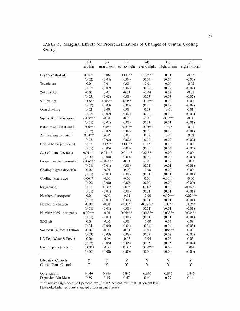
Table 5 presents similar results for cooling settings. Households that pay for central AC are

more likely to make changes to their cooling settings at any point in time during the day and also

between evening and night. They are less likely to do so however if they live in large apartment

buildings. Older residents are also more likely to make changes to their cooling settings. Most of

the other demographic coefficients are not statistically significant.

[ Table 5 about here ]

The picture that emerges from the heating and cooling results is one where households are more

likely to engage in some form of energy economizing behavior if they pay for their heating or cool-

ing. The results are somewhat stronger for heating than central cooling. Interestingly, the extent

to which households engage in this form of economizing behavior depends on the opportunities

for improving comfort available. Households living in colder areas are more likely to keep their

homes cooler but also more likely to keep their homes cooler at night than during in the evening

and morning. This suggests that the response to economic incentives may in fact be larger when

the opportunities for savings are more substantial.

18

5.1.3. Robustness to unobserved heterogeneity. We recognize that if there is unobserved hetero-

geneity across households that is somehow correlated with the decision of whether to pay for

heating or cooling, we may have an endogeneity concern. While it is plausible to us that whether

a housing contract includes the cost of heating or cooling is a secondary issue to more important

factors that individuals consider when choosing where to live, we feel it is still worthwhile to per-

form an additional robustness check. Our cross-sectional dataset does not allow for household

fixed or random effects in the previous regressions, but by focusing on within-day choices, we

can construct a panel dataset. Then, we can consider the choice to change heating and cooling

settings between morning and day, day and evening, evening and night and night and morning as

choices made by the same household during four consecutive choice occasions. This allows us to

include household-specific effects for these choices under the assumption that we observe choices

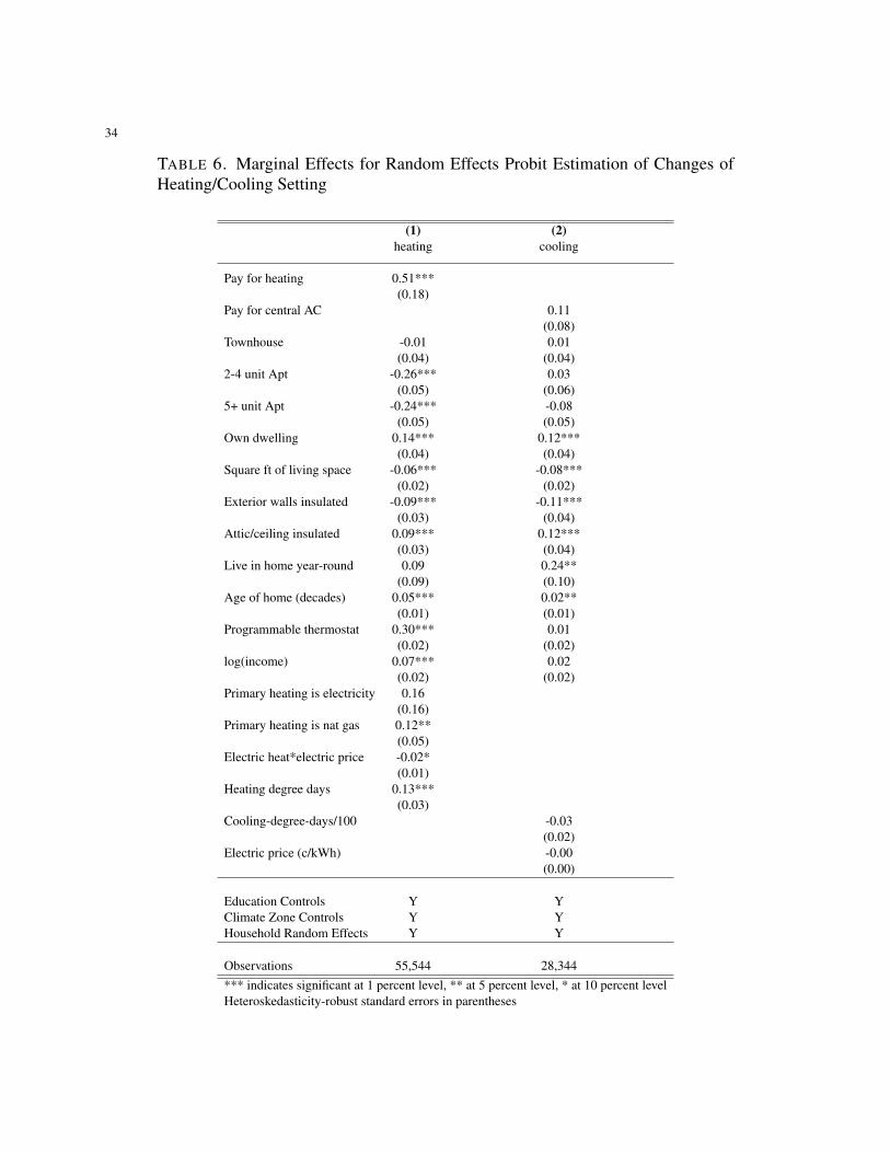
for T = 4 choice occasions. Table 6 reports the estimated marginal effects from a random effects

probit model.

[ Table 6 about here ]

The results presented in Table 6 suggest that our previous results are likely to be robust to

unobserved household-level heterogeneity. Households who pay for heating have a large and sta-

tistically significant propensity to adjust heating settings during the day. However, they are less

likely to adjust their heating settings if they live in apartment buildings. Households are more likely

to adjust their settings when they live in colder areas. Wealthier (and more educated) individuals

are more likely to optimize during the day. Similar but weaker results are obtained for cooling

decisions.

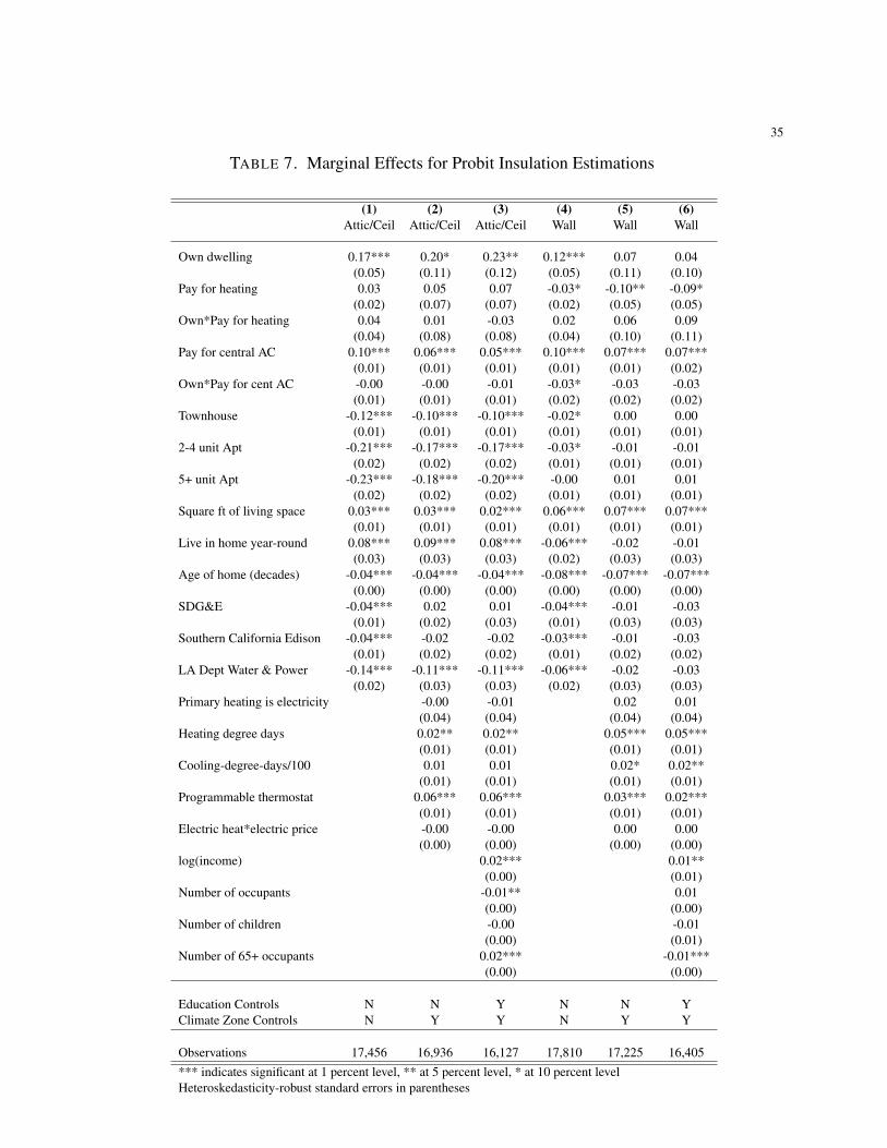
5.2. Insulation. In Table 7 we investigate the extent to which the presence of either attic/ceiling

insulation or exterior wall insulation in a home is related to whether the occupant owns the dwelling

19

(box (2) in Figure 1). We perform the estimation for both attic/ceiling insulation (first three

columns) and wall insulation (latter three columns), and we interact home ownership with pay-

ing for heating and central cooling.

[ Table 7 about here ]

Several of these results match our theoretical predictions well. Owner-occupied dwellings where

the resident pays for heating (box (1) in Figure 1) are roughly 20 percent more likely to be insulated

in the attic/ceiling. A joint test of the coefficients indicates that this result is statistically significant

to the 1 percent confidence level. Similarly, owner-occupied dwellings where the resident pays

for heating are roughly 13 percent more likely to be insulated in the exterior walls. This result is

statistically significant to the 10 percent level with a joint test of the coefficients. Owner-occupied

dwellings where the resident pays for central cooling are also roughly 20 percent more likely to be

insulated in the attic/ceiling – again a statistically significant result. Moreover, rented dwellings

where the resident pays for heating (box (2) of Figure 1) are 9 percent less likely to be insulated in

the exterior walls, a result statistically significant at the 10 percent level. Combined, these results

provide clear evidence for a split incentive issue in insulation that corresponds with the theoretical

predictions discussed above.

Some of the other results in Table 7 do not have as clear of an interpretation. For example, owner-

occupied dwellings where the resident does not pay for heating or cooling (box (3) in Figure 1) are

23 percent more likely to be insulated in the attic/ceiling. Owner-occupied dwellings where the

resident does not pay for heating or cooling are 4 percent more likely to be insulated in the exterior

walls, but this result is not statistically significant. Recall that there was not a strong theoretical

prediction for box (3) in Figure 1, for the result depended on the nature of the housing where

people own their dwelling but do not pay for their heating or cooling. Thus, we deem these results

20

as indicative that in these cases the building manager who provides and pays for the heating or

cooling was also involved in the construction of the building, and thus was more likely to ensure

that the dwelling was insulated.

In all cases insulation is more likely to be present in colder areas and in homes with a pro-

grammable thermostat. Larger homes tend to be better insulated and homes in Southern California

are more likely to lack insulation. This suggests that homeowners in colder areas are more likely

to insulate their dwelling. We also find that attic/ceiling insulation is less likely in multi-unit com-

plexes.

6. ENERGY SAVINGS AND EMISSIONS REDUCTIONS

What energy savings and emissions reductions could we anticipate if we found a way to entirely

correct these split incentive issues? We perform a series of back-of-the-envelope calculations to

get a sense of the magnitude of the energy savings and emissions reductions that could be achiev-

able from fully correcting each of the split incentive issues. The details of these calculations are

described in Appendix A. Throughout the calculations, we strive to make generous assumptions,

so that our estimates can be considered as a rough upper bound. We recognize that our back-of-

the-envelope methodology abstracts from some details, but we intend for it to captures the most

important factors of interest.

A primary finding is that the energy savings and emissions reductions from addressing the in-

sulation split incentive issue would be quite a bit larger than the corresponding savings from ad-

dressing the heating or cooling split incentive issue. This result is driven both by the number of

households that may be affected by the issue as well as the empirically estimated magnitude of the

issue.

21

We find that renters who use natural gas for heating and cooling would save roughly 605 ft3

of natural gas per year if the insulation split incentive issues was corrected for both wall and at-

tic/ceiling insulation. Just over half of this savings is from heating. For comparison purposes, the

sample average natural gas usage is 32,572 ft3 per year. Renters who use electricity for heating

and cooling would save roughly 21 kWh/year, with just over half of this savings from heating. The

sample average electricity usage (for all purposes, not just heating or cooling) is 4,048 kWh/year.

Since 75 percent of the households use natural gas for heating, and nearly 100 percent use elec-

tricity for cooling, the resulting energy savings for any given household will likely involve some

natural gas savings and some electricity savings. Looking at the magnitude of the savings, it is

clear that correcting the insulation split incentive problem may yield noticeable energy savings,

yet these savings are relatively small compared to the energy usage of an average household.

The corresponding carbon dioxide emissions reductions come out to 9.15 kg C/year per house-

hold. Extrapolating to the roughly 12 million households in California, the reductions are on the

order of 109,800 metric tons of CO2 per year. Just over half of these emissions reductions are

from wall insulation, and the rest are from attic or ceiling insulation improvements. Relative to

the 2007 residential (non-electric) CO2 emissions for California of 28 million metric tons of CO2,

these emissions reductions are extremely small. For a rough sense of the cost of improving the

insulation, the cost for fiberglass insulation is in the range of $0.30 per ft2 for R-13 or $0.90 per ft2

for R-30 insulation.12 So for a 1,000 ft2 roof, the difference is $900.

To calculate the energy savings possible from fully addressing the heating split incentive issue

we adjust the probability that households keep their temperature at each of the settings by the

empirically estimated marginal effects from the ordered probit regressions. We calculate that a 5

12These values are from the authors’ observations at the local Home Depot.

22

degree decrease in heating temperature setting corresponds to an energy savings of roughly 2,500

ft3 of natural gas per year or 75 kWh per year, depending on the heating fuel. Using these values

and extrapolating to California, we find emissions reductions of roughly 10,500 metric tons CO2

per year. Correcting for this issue with central cooling would yield a similar, but slightly smaller

emissions reduction.

The relatively small magnitude of emissions reductions from correcting the heating or cooling

split incentive issues is due both to the moderate behavioral changes in our empirical results and

to the fact that in our sample only 5 percent of Californians do not pay for their own heat (using

sample weights). While this small percentage may seem surprising, a comparison with the 2005

Residential Energy Consumption Survey (RECS) indicates that nationwide only about 5 percent

do not pay for electric heat, 4 percent do not pay for central cooling, and 11 percent do not pay for

natural gas heating. Thus, the RASS data on paying for heat in California appear quite reasonable,

and we feel comfortable that our back-of-the-envelope calculation gives a helpful sense of what

can be achieved.

7. CONCLUSIONS

This study lays out a conceptual framework to elucidate when and how split incentives could lead

to principal-agent problems in two important cases: (1) when owners pay for heating or cooling

and occupants face zero marginal cost for these energy services and (2) when occupants who pay

for heating or cooling and cannot perfectly observe the prior choice of insulation by the owner. We

test the theoretical implications in order to provide some of the first empirical evidence quantifying

the effects of split incentives in both situations.

23

We find some evidence that paying for heating affects the heating or cooling temperature setting.

We find stronger evidence that occupants who pay for heating change their heating setting more

often than those who do not. For example, those who pay for heating are 16 percent more likely to

turn down their heat at night. This suggests that those who are paying for heating are also thinking

much more about their heating bill and putting in more effort to reduce their heating bill. The

same split incentive issue also appears to hold for central air conditioning, although slightly less

strongly.

There is also a clear mapping between our theoretical and empirical results on a split incentive

issue relating to ownership of the dwelling and the degree to which the dwelling is insulated.

For example, if the dwelling is owner-occupied and the resident pays for heating or cooling, the

attic/ceiling is roughly 20 percent more likely to be insulated, and the exterior walls are roughly

13 percent more likely to be insulated. Both the insulation and heating/cooling results match the

theoretical predictions of our conceptual framework.

Given the amount of policy discussion about principal-agent problems in energy use, we found

it illustrative to calculate rough estimates of the energy savings and emissions reductions possible

from completely correcting these split incentive issues. Our estimates indicate that the split in-

centive issue relating to insulation leads to greater additional energy consumption and emissions

than the split incentive issue from not paying for energy use. Specifically, split incentive problems

may increase total natural gas use by as much as 2 percent and total electricity use by as much as

1 percent. The emissions reductions from fully addressing the insulation split incentive issue in

California are estimated to be roughly 109,800 metric tons of CO2 per year, while the reductions

from fully addressing the heating split incentive issue in California are estimated to be 10,500

metric tons of CO2 per year. This difference is driven both by our empirical estimates and by the

24

much larger number of households occupied by renters who pay for energy use (box (2) in Figure

1) than the number of households where the occupant does not pay for energy use (boxes (3) and

(4) in Figure 1). Importantly, our estimates are quite small relative to total residential emissions,

suggesting that if the policy goal is to reduce emissions substantially, split incentive issues should

be a sidelight to a broader climate change policy.

Of course, even if the residential split incentive issues are not large relative to total emissions,

there may be low-cost targeted policies that could improve economic efficiency by helping to

address these issues. For instance, since the insulation issue inherently involves asymmetric infor-

mation, information programs, such as required insulation quality disclosure on rental leases, may

be a cost-effective approach. It may also be possible that providing consumers real-time feedback

on electricity use and emissions may lead households motivated by environmental concerns to ex-

ert more effort to save energy. Minimum standards on new rental units may cost-effectively help

to address the insulation split-incentive issue. Analyzing the effects of these policies on reducing

the importance of split incentive issues in the owner-occupant relationship is a promising area of

future research.

ACKNOWLEDGMENTS

We are grateful for the excellent research assistance from Kester Tong, Paul Ma, Rachid ElKhattabi, Annie Xuanwen, Paris Georgoudis, Binying Liu. We would also like to thank LarryGoulder, Danny Cullenward, Sebastien Houde, Arthur van Benthem, Anant Sudarshan, and AdamMillard-Ball for comments and suggestions. We thank the California Public Utilities Commissionfor providing the RASS dataset and Glen Sharp for his assistance with understanding the data. Wewould like to thank the Precourt Energy Efficiency Center for the funding making this researchpossible.

25

REFERENCES

ALCHIAN, A., AND H. DEMSETZ (1972): “Production, Information Costs, and Economic Organization,” AmericanEconomic Review, 62, 777–795.

ARROW, K. (1963): Social Choice and Individual Values. Wiley: New York.BLUMSTEIN, C., B. KRIEG, L. SCHIPPER, AND C. YORK (1980): “Overcoming Social and Institutional Barriers toEnergy Conservation,” Energy, 5(4), 355–371.

BORENSTEIN, S. (2008): “Equity Effects of Increasing-Block Electricity Pricing,” University of California EnergyInstitute CSEM WP 180.

(2009): “To What Electricity Price Do Consumers Respond? Residential Demand Elasticity UnderIncreasing-Block Pricing,” UC Berkeley Working Paper.

CALIFORNIA ENERGY COMMISSION (2003): “California’s Electricity Generation and Transmission InterconnectionNeeds Under Alternative Scenarios,” Discussion paper, Prepared by Electric Power Group, LLC.

DAVIS, L. (2009): “Evaluating the Slow Adoption of Energy Efficient Investments: Are Renters Less Likely to HaveEnergy Efficient Appliances?,” UC-Berkeley mimeo.

EIA (2008): “Annual Energy Outlook 2008,” .FISHER, A., AND M. ROTHKOPF (1989): “Market Failure and Energy Policy: A Rationale for Selective Conserva-tion,” Energy Policy, 17(4), 397–406.

GILLINGHAM, K., R. NEWELL, AND K. PALMER (2006): “Energy Efficiency Policies: A Retrospective Examina-tion,” Annual Review of Environment and Resources, 31, 193–237.

(2009): “Energy Efficiency Economics and Policy,” Annual Review of Resource Economics, 1, 597–619.GROSSMAN, S., AND O. HART (1982): Economics of Information and Uncertainty ,chap. Corporate Financial Struc-ture and Managerial Incentives, (ed) J McCall. University of Chicago Press: Chicago, IL.

INTERNATIONAL ENERGY AGENCY (2007): “Mind The Gap: Quantifying Principal-Agent Problems in EnergyEfficiency,” Discussion paper, OECD/IEA.

ITO, K. (2010): “How Do Consumers Respond to Nonlinear Pricing? Evidence from Household Electricity Demand,”UC-Berkeley Working Paper.

JAFFE, A., AND R. STAVINS (1994): “The Energy Efficiency Gap: What Does it Mean?,” Energy Policy, 22(10),804–810.

JENSEN, M., AND W. MECKLING (1976): “Theory of the Firm: Managerial Behavior, Agency Costs and OwnershipStructure,” Journal of Financial Economics, 3, 305–360.

LAFFONT, J.-J., AND D. MARTIMORT (2001): The Theory of Incentives: The Principal-Agent Model. PrincetonUniversity Press.

LEVINSON, A., AND S. NIEMANN (2004): “Energy Use by Apartment Tenants When Landlords Pay for Utilities,”Resource and Energy Economics, 26(1), 51–75.

MURTISHAW, S., AND J. SATHAYE (2006): “Quantifying the Effect of the Principal-Agent Problem on US EnergyUse,” Discussion paper, Lawrence Berkeley National Laboratory, LBNL-59773.

NADEL, S. (2002): “Appliance and Equipment Efficiency Standards,” Annual Review of Energy and the Environment,27, 159–192.

NEW YORK TIMES (2010): “Air-Conditioners That Run When Nobodys Home,” August 15.SPENCE, M., AND R. ZECKHAUSER (1971): “Insurance, Information, and Individual Action,” American EconomicReview, 61(2), 380–387.

US CENSUS BUREAU (2010): “Current Population Survey/Housing Vacancy Survey,” .

26

APPENDIX A. ENERGY SAVINGS AND EMISSIONS REDUCTIONS CALCULATIONS

This appendix describes the assumptions used in the back-of-the-envelope calculations of theenergy savings and emissions reductions. All calculations use the sample weights included theRASS dataset. First, we describe the calculations for an estimate of the energy savings fromaddressing the insulation split incentive issue, then move on to energy savings from the heating splitincentive issue, and finally describe the conversion factors used to calculate emissions reductions.

The methodology for calculating energy savings from correcting the insulation split incentiveissue is based on the following physical relationship:

HL = TD · A/R,where HL is the rate of heat loss, TD is the differential between the inside and outside tem-

perature, A is the surface area by which heat can escape, and R is the R-value of the insulation (ameasure of insulation quality). To calculate the temperature differential, we first find daily data onthe high, low, and average temperature at test stations in each county in California from the UCIPM Online: Statewide Integrated Pest Management Program (www.ipm.ucdavis.edu). We use theaverage high-low-average temperature for each county in California and match these by county tothe observations in our dataset. For the three counties that did not have a test station, we choosean adjacent county that to the best of our knowledge has a similar climate. We then calculate thetemperature difference between the observed indoor temperature in each time of day, and the hightemperature for daytime, the low temperature for nighttime, and the average temperature for morn-ing and evening. This gives us a temperature difference for each day of the year and for each ofthe four times-of-day.

To calculate the surface area in square feet, we make the following assumptions: single-familyhomes are square and have all four walls exposed to the outside, townhouses are rectangles andhave two walls exposed to the outside, 2-4 unit apartments are square and have two walls exposedto the outside, and 5+ unit apartments are square and have one wall exposed to the outside. We thenuse the observed square footage of the dwelling, observed number of stories of the dwelling, andan assumed height of 12 feet per story to calculate the wall area and ceiling area. For single-familyhomes and townhouses, we assume that the roof has a pitch such that the surface area is 1.2 timesa flat roof.

We take R-values of the insulated apartments from the Department of Energy suggested insula-tion levels for California. These are R-values of 5 for walls and 30 for attics/ceilings. For poorlyinsulated dwellings, we use an estimate of 3 for walls and 9 for attics/ceilings. We can then cal-culate the rate of heat loss by time of day and day of year. These estimates are then aggregatedfor both heating and cooling and converted to cubic feet of natural gas or kWh of electricity. Thenwe use our marginal effects from Table 7 to calculate how many more observations in our samplewould be insulated if the split incentive issue did not exist. In other words, for renters we increasedthe sample probability of being insulated by 20 percent for attic/ceiling insulation and 13 percentfor wall insulation. We then can calculate the total energy savings (in natural gas or electricity) be-tween the current case and the counterfactual where the insulation split incentive issue was entirelycorrected.

27

To find the energy savings from addressing the heating split incentive issue, we begin by per-forming a simple linear fit of the heating setting at each time of day on the household yearly naturalgas use and all of the covariates used in Table 5 for households that use natural gas. For householdsthat use electricity, we perform a similar linear fit on the household yearly electricity consumption.For all four time periods, the result for natural gas indicates that a one degree increase in heatingsetting corresponds to roughly 2,500 ft3 per year in additional natural gas use. For electricity, theestimation result indicates that a one degree increase in heating setting corresponds to roughly 75kWh per year in additional electricity use.

We then use a similar methodology as for insulation, by focusing on those who do not pay forheat and changing the sample probability of being in one of the heating setting categories by themarginal effects estimated in the ordered probit estimation. The calculation is done separately forthose who use natural gas and electricity. These give a result of the number in the sample whocurrently are in some (e.g., high) heating setting but in the counterfactual when the split incentiveissue is corrected, would be in a different (e.g., lower) heating setting. This number is multipliedby the energy savings to get the total energy savings. Note that when our sample is extrapolatedout to the population of California, the data indicate that 95 percent of residents pay for heat attheir dwelling. So the resulting energy savings and carbon dioxide emissions reflect this relativelysmall number who do not pay for heating. On the other hand, roughly 25 percent of the dwellingsare rented.

Carbon dioxide emissions reductions are based on carbon intensity of natural gas (1 m3 = 0.49 kgcarbon) for those who use natural gas, and the average carbon intensity of electricity in California(1 MJ = 0.01 kg carbon) based on estimates of the primary energy sources used California in 2003(California Energy Commission 2003). To the extent that California’s electric power sector isfurther de-carbonizing, this estimate is an over-estimate.

28

FIGURE 1. Matrix of possible avenues for split incentives in the owner-occupantrelationship. The agent making the hidden action in the owner-occupant problem isindicated in parentheses.

29

TABLE 1. Summary Statistics

Variable Mean Std Dev Min Max NHeating/Cooling Setting, Higher ⇒ Warmer

Heating setting in morning 3.67 0.99 1 6 13,641Heating setting in day 3.34 1.10 1 6 10,857Heating setting in evening 3.81 0.90 1 6 14,120Heating setting at night 3.04 1.16 1 6 11,085Central cooling setting in morning 4.42 1.75 1 6 8,732Central cooling setting in day 3.81 1.69 1 6 8,732Central cooling setting in evening 3.51 1.62 1 6 8,732Central cooling setting at night 4.48 1.74 1 6 8,732

Dwelling TypeLive in single family homes 0.66 0.47 0 1 20,933Live in townhouses 0.09 0.29 0 1 20,933Live in 2-4 unit apartments 0.08 0.27 0 1 20,933Live in 5+ unit apartments 0.16 0.37 0 1 20,933

Dwelling CharacteristicsOwn dwelling (not renting) 0.73 0.45 0 1 20,604Exterior walls insulated 0.73 0.44 0 1 18,418Attic and ceiling insulated 0.76 0.43 0 1 18,062House square footage (1,000 ft2) 1.56 0.81 0.2 6 20,905Age of dwelling (years) 33.67 18.02 0 68 20,933Own a spa 0.11 0.32 0 1 20,933Own a pool 0.09 0.29 0 1 20,933Live in home year-round 0.98 0.14 0 1 20,933Heating degree days (65 degree) 2.09 0.81 0.98 5.3 20,933Cooling degree days (65 degree) 0.88 0.77 0 4.3 20,933

Heating System CharacteristicsPay for heating 0.95 0.21 0 1 20,772Pay for central cooling 0.45 0.50 0 1 20,736Primary heating is electricity 0.12 0.32 0 1 19,960Electric price 14.92 4.00 7.3 25.8 20,933Primary heating is natural gas 0.81 0.39 0 1 19,968Primary heating is bottled gas 0.04 0.20 0 1 19,968Heating programmable thermostat 0.35 0.48 0 1 20,933Heating system age (years) 16.58 12.49 1 40 18,093Central cool programmable thermostat 0.24 0.43 0 1 20,933Central cool system age (years) 11.54 9.04 1 40 9,129

Resident CharacteristicsHousehold income (dollars) 64,878 45,995 4,272 431,189 20,904Number living in household 2.67 1.55 1 10 20,345Number of children 0.69 1.14 0 8 20,344Number of seniors 0.46 0.76 0 8 20,345

UtilityAnnual electricity consumption 5,948 4,194 0 71,268 20,518PG&E 0.44 0.50 0 1 20,933SDG&E 0.12 0.33 0 1 20,933SCE 0.37 0.48 0 1 20,933LADWP 0.07 0.25 0 1 20,933

30

TABLE 2. Cross-tabulations Corresponding to Figure 1

Own dwelling Rent dwelling TotalPay for heating 7,742 2,242 9,984Do not pay for heating 50 209 259Total 7,792 2,451 10,243

Own dwelling Rent dwelling TotalPay for central cooling 4,902 1,162 6,064Do not pay for central cooling 1,506 1,092 2,598Total 6,408 2,254 8,662Note: the top matrix is restricted to the heating subsample; the bottommatrix is restricted to the cooling subsample.

31

TABLE 3. Morning Heating Ordered Probit Marginal Effects

(1) (2) (3) (4) (5) (6)below 55 55-60 61-65 66-70 71-75 over 75

Pay for heating 0.027** 0.077 0.159 -0.009 -0.175 -0.079(0.012) (0.056) (0.195) (0.219) (0.269) (0.212)

Pay & ext walls insulated 0.010 0.022 0.030 -0.028 -0.027 -0.007(0.028) (0.064) (0.091) (0.076) (0.084) (0.022)

Pay & attic/ceiling insulated -0.294 -0.223*** -0.054 0.405* 0.140*** 0.026**(0.388) (0.059) (0.146) (0.237) (0.052) (0.013)

Own dwelling 0.005 0.010 0.013 -0.014 -0.012 -0.003(0.003) (0.007) (0.009) (0.008) (0.008) (0.002)

Square ft of living space 0.003** 0.007** 0.009** -0.009** -0.008** -0.002**(0.001) (0.003) (0.004) (0.004) (0.003) (0.001)

Exterior walls insulated -0.008 -0.017 -0.020 0.023 0.018 0.004(0.037) (0.072) (0.082) (0.104) (0.072) (0.015)

Attic/ceiling insulated 0.051** 0.131*** 0.264** 0.074 -0.302** -0.219(0.022) (0.046) (0.108) (0.271) (0.118) (0.328)

Live in home year-round -0.008 -0.015 -0.017 0.021 0.015 0.003(0.010) (0.019) (0.021) (0.028) (0.018) (0.004)

Age of home (decades) 0.002*** 0.003*** 0.004*** -0.005*** -0.004*** -0.001***(0.001) (0.001) (0.002) (0.002) (0.001) (0.000)

Primary heating is electricity 0.022 0.040 0.042 -0.059 -0.037 -0.008(0.022) (0.036) (0.030) (0.056) (0.027) (0.005)

Primary heating is nat gas -0.007* -0.014** -0.017** 0.020* 0.015** 0.003**(0.004) (0.007) (0.008) (0.010) (0.007) (0.002)

Heating degree days 0.005** 0.011** 0.014** -0.015** -0.012** -0.003**(0.002) (0.004) (0.006) (0.006) (0.005) (0.001)

Programmable thermostat -0.009*** -0.018*** -0.022*** 0.024*** 0.020*** 0.005***(0.002) (0.004) (0.005) (0.006) (0.005) (0.001)

Electric heat*electric price -0.001 -0.002 -0.003 0.003 0.003 0.001(0.001) (0.002) (0.002) (0.002) (0.002) (0.000)

log(income) -0.002 -0.004 -0.005 0.005 0.004 0.001(0.002) (0.004) (0.004) (0.005) (0.004) (0.001)

Number of occupants -0.000 -0.001 -0.001 0.001 0.001 0.000(0.001) (0.002) (0.003) (0.003) (0.003) (0.001)

Number of children -0.003* -0.006* -0.007* 0.008* 0.006* 0.001*(0.002) (0.003) (0.004) (0.005) (0.004) (0.001)

Number of 65+ occupants -0.010*** -0.020*** -0.026*** 0.028*** 0.023*** 0.005***(0.001) (0.003) (0.004) (0.004) (0.003) (0.001)

Utility Controls Y Y Y Y Y YEducation Controls Y Y Y Y Y YClimate Zone Controls Y Y Y Y Y YObservations 6,060 6,060 6,060 6,060 6,060 6,060Pr(setting) 3.2 9.9 25.9 48.8 10.4 1.68*** indicates significant at 1 percent level, ** at 5 percent level, * at 10 percent levelHeteroskedasticity-robust standard errors in parentheses

32

TABLE 4. Marginal Effects for Probit Estimations of Changes of Heating Setting

(1) (2) (3) (4) (5) (6)anytime mrn to evn evn to night evn > night night to mrn night < morn

Pay for heating 0.11** 0.06 0.16** 0.09 0.15** 0.10(0.05) (0.06) (0.07) (0.07) (0.07) (0.07)

Townhouse -0.01 0.02 -0.01 0.00 -0.01 -0.03(0.01) (0.02) (0.02) (0.02) (0.02) (0.02)

2-4 unit Apt -0.08*** -0.05** -0.05** -0.05** -0.10*** -0.09***(0.02) (0.02) (0.02) (0.02) (0.02) (0.02)

5+ unit Apt -0.08*** -0.03 -0.06*** -0.05*** -0.08*** -0.10***(0.02) (0.02) (0.02) (0.02) (0.02) (0.02)

Own dwelling 0.01 0.01 0.04** 0.07*** 0.03** 0.07***(0.01) (0.01) (0.01) (0.02) (0.02) (0.02)

Square ft of living space -0.02*** -0.01* -0.00 0.00 -0.00 0.01(0.00) (0.01) (0.01) (0.01) (0.01) (0.01)

Exterior walls insulated -0.03*** -0.02* -0.03*** -0.05*** -0.02* -0.03**(0.01) (0.01) (0.01) (0.01) (0.01) (0.01)

Attic/ceiling insulated 0.00 -0.01 0.04*** 0.07*** 0.03*** 0.06***(0.01) (0.01) (0.01) (0.01) (0.01) (0.01)

Live in home year-round -0.01 -0.03 0.03 0.01 -0.01 -0.01(0.03) (0.04) (0.04) (0.04) (0.04) (0.04)

Age of home (decades) 0.02*** 0.00* 0.02*** 0.02*** 0.01*** 0.02***(0.00) (0.00) (0.00) (0.00) (0.00) (0.00)

Primary heating is electricity 0.04 0.09 0.01 -0.00 0.02 -0.02(0.04) (0.06) (0.06) (0.06) (0.06) (0.07)

Primary heating is nat gas -0.01 0.04** 0.03 0.02 0.04** 0.02(0.01) (0.02) (0.02) (0.02) (0.02) (0.02)

Heating degree days 0.04*** 0.01 0.05*** 0.06*** 0.04*** 0.05***(0.01) (0.01) (0.01) (0.01) (0.01) (0.01)

Programmable thermostat 0.03*** -0.04*** 0.09*** 0.11*** 0.09*** 0.12***(0.01) (0.01) (0.01) (0.01) (0.01) (0.01)

Electric heat*electric price -0.00* -0.00 -0.00 -0.00 -0.00 -0.00(0.00) (0.00) (0.00) (0.00) (0.00) (0.00)

log(income) -0.00 -0.01 0.02** 0.03*** 0.00 0.01(0.01) (0.01) (0.01) (0.01) (0.01) (0.01)

Number of occupants -0.01* 0.00 -0.02*** -0.04*** -0.01*** -0.03***(0.00) (0.00) (0.00) (0.01) (0.00) (0.01)

Number of children -0.00 -0.01 -0.00 -0.01 0.01 0.00(0.00) (0.01) (0.01) (0.01) (0.01) (0.01)

Number of 65+ occupants 0.02*** -0.01* 0.04*** 0.06*** 0.06*** 0.09***(0.00) (0.01) (0.01) (0.01) (0.01) (0.01)

SDG&E -0.03 -0.01 -0.01 -0.02 0.01 0.03(0.03) (0.03) (0.03) (0.03) (0.03) (0.03)

Southern California Edison -0.01 0.01 -0.00 -0.02 -0.00 -0.00(0.02) (0.03) (0.03) (0.03) (0.03) (0.03)

LA Dept Water & Power -0.02 -0.00 -0.04 -0.06 -0.00 -0.03(0.03) (0.04) (0.04) (0.04) (0.04) (0.04)

Education Controls Y Y Y Y Y YClimate Zone Controls Y Y Y Y Y Y

Observations 13,392 13,392 13,392 13,392 13,392 13,392Dependent Var Mean 0.81 0.39 0.64 0.57 0.58 0.49*** indicates significant at 1 percent level, ** at 5 percent level, * at 10 percent levelHeteroskedasticity-robust standard errors in parentheses

33

TABLE 5. Marginal Effects for Probit Estimations of Changes of Central CoolingSetting

(1) (2) (3) (4) (5) (6)anytime mrn to evn evn to night evn < night night to mrn night > morn

Pay for central AC 0.09** 0.06 0.13*** 0.12*** 0.01 -0.03(0.02) (0.04) (0.04) (0.04) (0.04) (0.03)

Townhouse -0.01 0.01 0.01 -0.01 0.00 -0.02(0.02) (0.02) (0.02) (0.02) (0.02) (0.02)

2-4 unit Apt -0.01 0.01 -0.01 -0.04 0.02 -0.01(0.03) (0.03) (0.03) (0.03) (0.03) (0.02)

5+ unit Apt -0.06** -0.06** -0.05* -0.06** 0.00 0.00(0.03) (0.03) (0.03) (0.03) (0.02) (0.02)

Own dwelling 0.02 0.00 0.03 0.03 -0.01 0.01(0.02) (0.02) (0.02) (0.02) (0.02) (0.02)

Square ft of living space -0.03*** -0.01 -0.02 -0.01 -0.02** -0.00(0.01) (0.01) (0.01) (0.01) (0.01) (0.01)

Exterior walls insulated -0.06*** -0.03* -0.04** -0.05** -0.02 -0.01(0.02) (0.02) (0.02) (0.02) (0.02) (0.01)

Attic/ceiling insulated 0.04** 0.04* 0.03 0.02 -0.01 -0.02(0.02) (0.02) (0.02) (0.02) (0.02) (0.02)

Live in home year-round 0.07 0.12** 0.14*** 0.11** 0.06 0.00(0.05) (0.05) (0.05) (0.05) (0.04) (0.04)

Age of home (decades) 0.01*** 0.01*** 0.01*** 0.01*** 0.00 0.00(0.00) (0.00) (0.00) (0.00) (0.00) (0.00)

Programmable thermostat -0.06*** -0.04*** -0.01 -0.01 0.02 0.02*(0.01) (0.01) (0.01) (0.01) (0.01) (0.01)

Cooling-degree-days/100 -0.00 -0.01 -0.00 -0.00 0.00 0.00(0.01) (0.01) (0.01) (0.01) (0.01) (0.01)

Cooling system age -0.00*** -0.00 -0.00 0.00 -0.00*** -0.00(0.00) (0.00) (0.00) (0.00) (0.00) (0.00)

log(income) 0.01 0.03** 0.02* 0.02* 0.00 -0.02**(0.01) (0.01) (0.01) (0.01) (0.01) (0.01)

Number of occupants -0.01 -0.00 -0.01 -0.00 -0.02*** -0.02***(0.01) (0.01) (0.01) (0.01) (0.01) (0.01)

Number of children -0.00 -0.01 -0.02** -0.02*** 0.02** 0.02**(0.01) (0.01) (0.01) (0.01) (0.01) (0.01)

Number of 65+ occupants 0.02*** -0.01 0.05*** 0.04*** 0.03*** 0.04***(0.01) (0.01) (0.01) (0.01) (0.01) (0.01)

SDG&E -0.04 -0.06 0.01 -0.00 0.05 0.03(0.04) (0.04) (0.04) (0.04) (0.04) (0.03)

Southern California Edison -0.02 -0.03 -0.01 -0.03 0.08*** 0.03(0.03) (0.03) (0.03) (0.03) (0.03) (0.02)

LA Dept Water & Power -0.06 -0.08 -0.05 -0.04 0.06 0.05(0.05) (0.05) (0.05) (0.05) (0.05) (0.04)

Electric price (c/kWh) -0.00** -0.00 -0.00* -0.00** 0.00 0.00*(0.00) (0.00) (0.00) (0.00) (0.00) (0.00)

Education Controls Y Y Y Y Y YClimate Zone Controls Y Y Y Y Y Y

Observations 6,846 6,846 6,846 6,846 6,846 6,846Dependent Var Mean 0.69 0.45 0.47 0.40 0.27 0.14*** indicates significant at 1 percent level, ** at 5 percent level, * at 10 percent levelHeteroskedasticity-robust standard errors in parentheses

34

TABLE 6. Marginal Effects for Random Effects Probit Estimation of Changes ofHeating/Cooling Setting

(1) (2)heating cooling

Pay for heating 0.51***(0.18)

Pay for central AC 0.11(0.08)

Townhouse -0.01 0.01(0.04) (0.04)

2-4 unit Apt -0.26*** 0.03(0.05) (0.06)

5+ unit Apt -0.24*** -0.08(0.05) (0.05)

Own dwelling 0.14*** 0.12***(0.04) (0.04)

Square ft of living space -0.06*** -0.08***(0.02) (0.02)

Exterior walls insulated -0.09*** -0.11***(0.03) (0.04)

Attic/ceiling insulated 0.09*** 0.12***(0.03) (0.04)

Live in home year-round 0.09 0.24**(0.09) (0.10)

Age of home (decades) 0.05*** 0.02**(0.01) (0.01)

Programmable thermostat 0.30*** 0.01(0.02) (0.02)

log(income) 0.07*** 0.02(0.02) (0.02)

Primary heating is electricity 0.16(0.16)

Primary heating is nat gas 0.12**(0.05)

Electric heat*electric price -0.02*(0.01)

Heating degree days 0.13***(0.03)

Cooling-degree-days/100 -0.03(0.02)

Electric price (c/kWh) -0.00(0.00)

Education Controls Y YClimate Zone Controls Y YHousehold Random Effects Y Y

Observations 55,544 28,344*** indicates significant at 1 percent level, ** at 5 percent level, * at 10 percent levelHeteroskedasticity-robust standard errors in parentheses

35

TABLE 7. Marginal Effects for Probit Insulation Estimations

(1) (2) (3) (4) (5) (6)Attic/Ceil Attic/Ceil Attic/Ceil Wall Wall Wall

Own dwelling 0.17*** 0.20* 0.23** 0.12*** 0.07 0.04(0.05) (0.11) (0.12) (0.05) (0.11) (0.10)

Pay for heating 0.03 0.05 0.07 -0.03* -0.10** -0.09*(0.02) (0.07) (0.07) (0.02) (0.05) (0.05)

Own*Pay for heating 0.04 0.01 -0.03 0.02 0.06 0.09(0.04) (0.08) (0.08) (0.04) (0.10) (0.11)

Pay for central AC 0.10*** 0.06*** 0.05*** 0.10*** 0.07*** 0.07***(0.01) (0.01) (0.01) (0.01) (0.01) (0.02)

Own*Pay for cent AC -0.00 -0.00 -0.01 -0.03* -0.03 -0.03(0.01) (0.01) (0.01) (0.02) (0.02) (0.02)

Townhouse -0.12*** -0.10*** -0.10*** -0.02* 0.00 0.00(0.01) (0.01) (0.01) (0.01) (0.01) (0.01)

2-4 unit Apt -0.21*** -0.17*** -0.17*** -0.03* -0.01 -0.01(0.02) (0.02) (0.02) (0.01) (0.01) (0.01)

5+ unit Apt -0.23*** -0.18*** -0.20*** -0.00 0.01 0.01(0.02) (0.02) (0.02) (0.01) (0.01) (0.01)

Square ft of living space 0.03*** 0.03*** 0.02*** 0.06*** 0.07*** 0.07***(0.01) (0.01) (0.01) (0.01) (0.01) (0.01)

Live in home year-round 0.08*** 0.09*** 0.08*** -0.06*** -0.02 -0.01(0.03) (0.03) (0.03) (0.02) (0.03) (0.03)

Age of home (decades) -0.04*** -0.04*** -0.04*** -0.08*** -0.07*** -0.07***(0.00) (0.00) (0.00) (0.00) (0.00) (0.00)

SDG&E -0.04*** 0.02 0.01 -0.04*** -0.01 -0.03(0.01) (0.02) (0.03) (0.01) (0.03) (0.03)

Southern California Edison -0.04*** -0.02 -0.02 -0.03*** -0.01 -0.03(0.01) (0.02) (0.02) (0.01) (0.02) (0.02)

LA Dept Water & Power -0.14*** -0.11*** -0.11*** -0.06*** -0.02 -0.03(0.02) (0.03) (0.03) (0.02) (0.03) (0.03)

Primary heating is electricity -0.00 -0.01 0.02 0.01(0.04) (0.04) (0.04) (0.04)

Heating degree days 0.02** 0.02** 0.05*** 0.05***(0.01) (0.01) (0.01) (0.01)

Cooling-degree-days/100 0.01 0.01 0.02* 0.02**(0.01) (0.01) (0.01) (0.01)

Programmable thermostat 0.06*** 0.06*** 0.03*** 0.02***(0.01) (0.01) (0.01) (0.01)

Electric heat*electric price -0.00 -0.00 0.00 0.00(0.00) (0.00) (0.00) (0.00)

log(income) 0.02*** 0.01**(0.00) (0.01)

Number of occupants -0.01** 0.01(0.00) (0.00)

Number of children -0.00 -0.01(0.00) (0.01)

Number of 65+ occupants 0.02*** -0.01***(0.00) (0.00)

Education Controls N N Y N N YClimate Zone Controls N Y Y N Y Y

Observations 17,456 16,936 16,127 17,810 17,225 16,405*** indicates significant at 1 percent level, ** at 5 percent level, * at 10 percent levelHeteroskedasticity-robust standard errors in parentheses