Embed Size (px)
Citation preview

NeuroImage 86 (2014) 111–122
Contents lists available at ScienceDirect
NeuroImage
j ourna l homepage: www.e lsev ie r .com/ locate /yn img
SPoC: A novel framework for relating the amplitude of neuronaloscillations to behaviorally relevant parameters☆
Sven Dähne a,d,⁎, Frank C. Meinecke a, Stefan Haufe a,b, Johannes Höhne a, Michael Tangermann a,Klaus-Robert Müller a,b,c,d,e,⁎⁎, Vadim V. Nikulin c,d,⁎⁎⁎a Machine Learning Group, Department of Computer Science, Berlin Institute of Technology, Marchstr. 23, 10587 Berlin, Germanyb Bernstein Focus Neurotechnology, Berlin, Germanyc Neurophysics Group, Department of Neurology, Campus Benjamin Franklin, Charité University Medicine Berlin, 12203 Berlin, Germanyd Bernstein Center for Computational Neuroscience, Berlin, Germanye Department of Brain and Cognitive Engineering, Korea University, Anam-dong, Seongbuk-gu, Seoul 136-713, Republic of Korea
☆ This is an open-access article distributed under the tAttribution-NonCommercial-NoDerivativeWorks License,use, distribution, and reproduction in anymedium, provideare credited.⁎ Correspondence to: S. Dähne, Machine Learning Gr
Science, Berlin Institute of Technology, Marchstr. 23, 1058⁎⁎ Correspondence to: K.-R. Müller, Bernstein Focus Neu⁎⁎⁎ Correspondence to: V.V. Nikulin, Neurophysics GroCampus Benjamin Franklin, Charité University Medicine B
E-mail addresses: [email protected] (S. Dä[email protected] (K.-R.Müller), vadim.n
1053-8119/$ – see front matter © 2013 The Authors. Pubhttp://dx.doi.org/10.1016/j.neuroimage.2013.07.079
a b s t r a c t
a r t i c l e i n f oArticle history:Accepted 30 July 2013Available online 15 August 2013
Keywords:EEGMEGOscillationsSPoCSource power comodulationASSEP
Previously, modulations in power of neuronal oscillations have been functionally linked to sensory, motor andcognitive operations. Such links are commonly established by relating the power modulations to specific targetvariables such as reaction times or task ratings. Consequently, the resulting spatio-spectral representation issubjected to neurophysiological interpretation. As an alternative, independent component analysis (ICA) or alter-native decompositionmethods can be applied and the power of the componentsmay be related to the target var-iable. In this paperwe show that these standard approaches are suboptimal as thefirst does not take into accountthe superposition of many sources due to volume conduction, while the second is unable to exploit available in-formation about the target variable. To improve upon these approacheswe introduce a novel (supervised) sourceseparation framework called Source Power Comodulation (SPoC). SPoC makes use of the target variable in thedecomposition process in order to give preference to componentswhose power comodulateswith the target var-iable. We present two algorithms that implement the SPoC approach. Using simulations with a realistic headmodel, we show that the SPoC algorithms are able extract neuronal components exhibiting high correlation ofpower with the target variable. In this task, the SPoC algorithms outperform other commonly used techniquesthat are based on the sensor data or ICA approaches. Furthermore, using real electroencephalography (EEG) re-cordings during an auditory steady state paradigm, we demonstrate the utility of the SPoC algorithms byextracting neuronal components exhibiting high correlation of power with the intensity of the auditory input.Taking into account the results of the simulations and real EEG recordings, we conclude that SPoC representsan adequate approach for the optimal extraction of neuronal components showing coupling of power with con-tinuously changing behaviorally relevant parameters.
© 2013 The Authors. Published by Elsevier Inc. All rights reserved.
Introduction
Neural oscillations as measured by electro- and magnetoencepha-lography (EEG/MEG) have long been associated with sensory, motor,as well as cognitive processing (Buzsáki and Draguhn, 2004) and
erms of the Creative Commonswhich permits non-commerciald theoriginal author and source
oup, Department of Computer7 Berlin, Germany.rotechnology, Berlin, Germany.up, Department of Neurology,erlin, 12203 Berlin, Germany.e),[email protected] (V.V. Nikulin).
lished by Elsevier Inc. All rights reser
information transfer within the brain (Colgin et al., 2009; Womelsdorfand Fries, 2007).
In particular, it is widely believed that the amplitude/power modu-lation of these oscillations reflects the amount of spatial synchronizationamong neurons corresponding to different brain states (see (Riederet al., 2011) for a review).
Cognitive phenomena, that have been shown to correlate with bandpowermodulations, include e.g. attention (Başar et al., 1997; Bauer et al.,2006; Brovelli et al., 2005; Debener et al., 2003; Haegens et al., 2011a;Kaiser et al., 2006; Klimesch et al., 1998; Tallon-Baudry et al., 2005),memory encoding (Jensen et al., 2007; Klimesch, 1999; Osipova et al.,2006), vigilance in operational environments (Gevins et al., 1995;Holm et al., 2009), sleep stages (Darchia et al., 2007; Demanuele et al.,2012), perception (Gonzalez Andino et al., 2005; Jin et al., 2006;Makeig and Jung, 1996; Plourde et al., 1991; Thut et al., 2006), and deci-sion making (Haegens et al., 2011a, 2011b). In Transcranial MagneticStimulation research it has also been shown that the excitability of the
ved.

Fig. 1. Illustration of the problem setting. The unobservable source space signals (e.g. oscil-latory brain sources) are mixed to constitute the sensor space signals (e.g. EEG/MEG). Thetime course of the observed target variable z (e.g. stimulus intensity, reaction times) cor-responds to the power (or envelope) modulation of one of the sources.
1 The term noise sources subsumes all signals whose power is not related to the targetvariable. Specifically, this also includes actual brain sources which are different from e.g.measurement noise.
112 S. Dähne et al. / NeuroImage 86 (2014) 111–122
motor (Sauseng et al., 2009) and visual cortices (Romei et al., 2008),measured in terms of the amplitude of alpha oscillations, can also bepredictive of muscular motor evoked potentials and visual perception,respectively. In the field of Brain–Computer Interfaces (BCI), voluntarymodulation of EEG bandpower is used to control computer applications,such as text entry systems (Blankertz et al., 2007, 2008). It has beenshown recently that variability in BCI control-performance can be par-tially explained by the variability of spectral power across subjects(Blankertz et al., 2010), as well as within subjects (Grosse-Wentrupet al., 2011; Maeder et al., 2012).
For the purpose of this paper, we introduce the concept of a targetvariable (in the following denoted by z), which in principle can be anyscalar function of time. In the present neuroscience context, this targetvariablewill typically represent a behavioralmeasure as thefinal outputof the central nervous activity (e.g. reaction time, sensory detection,task rating, motor evoked potentials, etc.) or parameters of externalstimuli (e.g. when studying how amplitude modulation of neuronal os-cillations correlates with stimulus properties).
In general, we want to investigate the relation between EEG/MEGspectral power and such z variable in order to find a possible functionalrelationship between neuronal amplitude modulations and a behavioror stimulus. There are two standard approaches for establishing this re-lationship. In the first one, the spectral power is computed for eachchannel/sensor. A correlation to the target variable is then eitherassessed per channel, or using a multivariate regression approach. Inthe second approach, a linear projection from a sensor space into so-called source space is performed and further processing is performedtherein. As we will show later in detail, neither of the two common ap-proaches can be expected to yield optimal performance with EEG/MEGdata both in terms of themaximized correlation scores and the accuracywith which the underlying sources are extracted, thus limiting the sub-sequent neurophysiological interpretation of the results.
This paper explains the drawbacks of the conventional analyses andsuggests the novel Source Power Comodulation (SPoC) framework,which provides a theoretically sound andmathematically optimal solu-tion to the problem of relating EEG/MEG data to a given target variable.
The remainder of this article is organized as follows. In the Methodssection we recall the EEG/MEG forward model, discuss standard ap-proaches to obtaining correlations between band power and a targetvariable, and thereafter introduce the SPoC framework and two specificSPoC algorithms. The new approach is validated in simulations andwithreal world data, both described in the Validation section. Results arepresented in the Results section and we conclude with a discussion inthe Discussion section.
Methods
The generative model of EEG/MEG data
Electro- and magnetoencephalography are non-invasive techniquesallowing to measure macroscopic neuronal activity of the brain. WhileEEG measures scalp electrical potentials caused by neuronal activity,MEG measures the corresponding magnetic fields. Due to the volumeconduction in the head, the neuronal signals are spatially smearedwhile propagating to the EEG/MEG sensors. For the frequencies of inter-est in the analysis of brain oscillations (which are typically below1 kHz)this superposition is linear and instantaneous (Baillet et al., 2001;Nunezand Srinivasan, 2006; Parra et al., 2005). Thus, the following linearmodel holds for EEG/MEG data:
x tð Þ ¼ As tð Þ þ � tð Þ: ð1Þ
The vectorx tð Þ∈RNx here denotes themeasured data in sensor space(electrical potential or magnetic field) at time t, with Nx being the num-ber of recording channels. Themeasurement is a linear superposition ofNs sources (or components) with individual time courses si(t) and fixed
spatial patterns ai∈RNx , where s tð Þ ¼ s1 tð Þ;…; sNs tð Þð Þ⊤ contains thetime courses of the individual sources, A ¼ a1;…; aNs
� �contains the re-
spective spatial patterns in the columns, and �(t) models additive noise.Generally, the time courses of the sources are assumed to beuncorrelated and to have unit variance. Furthermore, the noise termcan be absorbed into the product As by adding additional columns inA and respective dimensions in s. Therefore we will omit the noiseterm in the following considerations.
Here we are interested in neural oscillations whose power timecourse comodulates (e.g. is correlated or anti-correlated)with an exter-nal variable. These neural oscillations are however not unambiguouslyobservable on the sensor level. Instead, they are superimposed withthe background brain activity and noise according to Eq. (1). This prob-lem setting is illustrated in Fig. 1.
Conventional approaches
Correlating the power of single sensorsDue to the sourcemixing, each sensor signal is generally a linear sum
of (1) the signal-of-interest s, whose power correlates with the targetvariable z and (2) noise1 sources n, whose power does not correlatewith the target. This implies that the correlation between z and theband power at any electrode is in fact a correlation between the powerof s with z, normalized by a term that grows monotonically with thesquared mixing coefficients of both the signal and noise sources, aswell as with the variances of their band power time courses (seeAppendix A). This illustrates the major drawbacks of the univariateapproach:
• Low signal-to-noise ratio. The true correlation between the power of sand z may be heavily underestimated in the presence of strong noisesources with high power.
• Lack of interpretability. The noise contribution may differ across elec-trodes, introducing a channel-specific bias in the correlation coeffi-cients. Hence, topographic maps of sensor-space correlation may notgive a good indication of where the signal-of-interest is strongestand are thereby hard to interpret in neurophysiological terms.
• Disregard of the generative model. It is practically impossible to disen-tangle signal and noise contributions by looking only at single elec-trodes. More generally, this approach does not provide a factorizationof the measurement x(t) into A and s(t) according to the generativelinear model of EEG/MEG data (see Eq. (1)).

Fig. 2. Illustration of different approaches to relating spectral power to a target variable.The input to all three approaches is the EEG/MEG data x(t) and the target variable z. Pro-cessing steps are organized from top to bottom. Left: an approach that is based on regres-sion. First, spectral power is computed on each sensor. Then the power time courses arelinearly combined to resemble z as close as possible. Middle: an approach that is basedon blind source separation (BSS) methods. A BSS method such as ICA tries to estimatethe sources prior to computation of spectral power. This approach is in line with the gen-erative EEG model and in principle could have the potential to find the true source. How-ever, BSS techniques do notmake use of the information contained in z and is bound to failfor low SNR or if the number of sources is larger than the number of channels. Right: Ournovel SPoC approach method makes use of z to guide the source estimation and to givepreference to sources whose power time course resembles z. Spectral power is computedon the estimated sources.
2 Working with epoched data instead of continuous data does not represent a loss ofgenerality, because all of the following derivations can be reformulated for continuous da-ta as well, provided that the target variable changes slowly enough. We choose to workwith epoched data because it resembles the format of data obtained in trial-basedexperiments.
113S. Dähne et al. / NeuroImage 86 (2014) 111–122
Correlating linear combinations of sensor powerInstead of correlating the band power of individual channels with z,
multivariate approaches can be applied, in which the target variable z iscorrelated with a weighted sum of the channel-wise band power. Usu-ally, the weights are chosen by regressing the band-power with the tar-get variable, thereby effectively maximizing the correlation. Using thisapproach, it is generally possible to achieve a high correlation (on thedata used to train the weight vector) if a sufficient amount of trainingdata is available. This may achieve superior performance compared tounivariate correlation in low signal-to-noise scenarios, thereby improv-ing upon the first point in the list above. However, in principle the othertwo drawbacks remain:
• Lack of interpretability. The regression weight vector does not neces-sarily contain neurophysiologically interpretable information aboutthe location of the underlying correlating source, because it is againa function of both the signal-of-interest and the noise (an explanationfor this can be found in (Blankertz et al., 2011)).
• Disregard of the generative model. Linearly regressing power valuesviolates the underlying generative model for EEG and MEG data,because it is linear in the ‘raw’ data, not in the squared data.
Blind source separation methodsA transformation into source space can be obtained by way of
so-called blind source separation methods (BSS). These methodsusually estimate a linear projection of the data x(t) onto a set ofweight vectors, which are represented here by the matrix W∈RNx�Ns ,where W ¼ w1;…;wi;…;wNs
� �, wi∈RNx , and Ns corresponds to the
number of estimated sources bsi tð Þ . In accordance with the literature,we refer to these weight vectors wi as spatial filters. Each of the spatialfilters is meant to extract the signal from one source while suppressingthe activity of the others, such that the resulting projected signal is a
close approximation of the original source signal, i.e. bsi tð Þ ¼ wi⊤x tð Þ .Band power correlations are then computed using bsi tð Þ instead ofxk(t). Popular BSS approaches, such as ICA, are in line with the genera-tive model of EEG/MEG and can thus in principle deliver results thatare interpretable within this model.
Note however that, by design, BSS methods are unsupervised learn-ing methods. They do not make use of a target variable z but optimizeother objectives instead, such as statistical independence, for example.This lack of optimizing for the desired target z leads to a suboptimal per-formance of BSS methods if:
• There is a low signal-to-noise ratio,• There are more sources than channels,• The target and the independence assumption contradict one another dueto dependencies between the sources.
The SPoC approach
The core idea of the SPoC framework is to (i) decompose the multi-variate EEG/MEGdata into a set of source components and (ii) to use theinformation contained in the target variable to guide thedecomposition.The result of this approach is a set of spatial filters,W, which directly op-timize the comodulation between the target variable z and the powertime course of the spatially filtered signal. Fig. 2 illustrates the contrastbetween regression of channel-wise band power features, BSSmethods,and the SPoC approach.
In the following subsection, we describe two algorithms that imple-ment the SPoC framework andwe refer to these twomethods as SPoCr2and SPoCλ. The difference between SPoCr2 and SPoCλ lies in the exactdefinition of comodulation between band power and z: SPoCr2 directlyoptimizes correlation, while SPoCλ optimizes covariance subject to ascaling constraint on the spatial filter. However, both algorithms invertthe generative model given in Eq. (1) prior to the computation of bandpower and thereby avoid pitfalls that were outlined above.
The SPoC algorithms
This subsection describes two possible ways to implement the SPoCidea outlined above.While the following definitions and derivations areimportant for understanding how the actual SPoC algorithms work, themathematically less inclined reader may skip ahead to the Validationsection without missing out on the main message of this paper.
Assumptions and definitionsWe assume that the EEG/MEG data x(t) has been band-pass filtered
in the frequency band of interest already. Thus, the power of theprojected signalw⊤x(t)within a given time interval iswell approximatedby the variance ofw⊤x(t) within that interval. We refer to such time in-tervals as epochs and assume that the EEG/MEG data can be divided upinto consecutive or overlapping epochs of suitable length.2 Epochs willbe indexed by the index e.
We assume the target variable z to only have a single value perepoch, which can be achieved by appropriate resampling. Furthermorewe assumewithout loss of generality that z has zeromean and unit var-iance, which can be achieved by normalization.
It is our goal to approximate the target variable zwith a quantity thatwe denote by ez, which depends on a spatial filterw. Let Var[w⊤x(t)](e)

114 S. Dähne et al. / NeuroImage 86 (2014) 111–122
denote the variance of w⊤x(t) in a given epoch e. This epoch-wisevariance of the projected signal will serve as the approximation of z.However, in the following we will slightly modify this quantitysuch that it has zero mean by definition. First, we note thatVar[w⊤x(t)](e) = w⊤C(e)w, where C(e) denotes the covariance matrixof x(t) in the eth epoch. Then we define the mean covariance matrix
C :¼ C eð Þh i; ð2Þ
where ⟨⋅⟩ denote the average across epochs. With these definitions wecan now define our quantity of interest as
ez eð Þ :¼ Var w⊤x tð Þh i
eð Þ−w⊤Cw¼ w⊤ C eð Þ−Cð Þw:
ð3Þ
Accordingly, the first twomoments ofez can be expressed in terms ofthe weight vector and epoch-wise covariance matrices as:
ez eð Þ� � ¼ w⊤ C eð Þ−Cð ÞwD E
¼⊤ C eð Þh iw−w⊤Cw¼ w⊤Cw−w⊤Cw¼ 0
ð4Þ
and
Var ez eð Þ� � ¼ ez eð Þ− ez eð Þ� �� �2D Ew⊤ C eð Þ−Cð Þw
� 2 �
:ð5Þ
Finally, we define the matrix
Cz :¼ C eð Þz eð Þh i; ð6Þ
which helps to conveniently express the covariance between ez and z as
Cov ez eð Þ; z eð Þ� � ¼ ez eð Þ− ez eð Þ� �� �z eð Þ− z eð Þh ið Þ� �
¼ w⊤ C eð Þ−Cð Þw�
z eð ÞD E
¼ w⊤ C eð Þz eð Þh iw− w⊤Cw�
z eð Þh i¼ w⊤Czw;
ð7Þ
where in the transition from line 1 to line 2 of this equation wehave used the fact that ez eð Þ� � ¼ z eð Þh i ¼ 0and substituted the definitionforez eð Þ. The next line is the result of factoring out. Finally, we made useof ⟨z(e)⟩ = 0 again and applied the definition for Cz, given in Eq. (6).
In the following subsections we formulate the objectives optimizedby the two algorithms that implement the SPoC approach. For ease ofnotation, the derivations are given for a single weight vector w∈RNx ,but generalize naturally to multiple filters providing a full-rank decom-positions of the data matrix.
Optimizing source power correlationWe are interested in positive as well as negative correlations and
hence choose to maximize the squared correlation between z and ez .We refer to this SPoC algorithm as SPoCr2 and maximize the followingobjective function:
f r2 ¼ Corr ez eð Þ; z eð Þ� �2¼ Cov ez eð Þ; z eð Þ� �2
Var ez eð Þ� �Var z eð Þ½ �
¼w⊤Czw
� 2
w⊤ C eð Þ−Cð Þw� 2
� :
ð8Þ
In the last equality of Eq. (8) we have used Eqs. (7) and (5), and the factthat Var[z(e)] = 1.
Theweight vectorw thatmaximizes fr2 cannot be found analytically.It should therefore be found using iterative optimization methods suchas gradient descent for example.
Optimizing source power covarianceHere we approximate the previous objective function by optimizing
the covariance betweenez and z. As wewill show shortly, this leads to anobjective function that has a number of computationally desirably prop-erties. We refer to this algorithm as SPoCλ. Unlike the correlation, thecovariance is affected by the scaling of its arguments. Thus far we haveassumed z to have zero mean and unit variance, i.e. that the scaling ofz is limited. Since we have only assumed ez to have zero mean, it is fur-thermore necessary to limit the scaling of ez. In SPoCλ we impose a con-straint on the norm of w and thereby limit the scaling of ez. Specificallywe choose the constraint such that the output of the spatial filter hasunit variance.With these definitionswe arrive at the followingobjectivefunction:
f λ ¼ Cov ez eð Þ; z eð Þ� � ¼ w⊤Czw; ð9Þ
with respect to the following norm constraint:
Var w⊤x tð Þh i
¼ w⊤Cw¼! 1: ð10Þ
This constraint optimization problem can be solved using themethod ofLagrange multipliers. Setting the first derivative of the correspondingLagrangian to zero leads to the following generalized eigenvalueequation:
Czw ¼ λCw; ð11Þ
where the eigenvalue λ corresponds to the value of fλ evaluated at therespective eigenvector w. Thus λ can directly be interpreted as the co-variance between ez and z.
Finding the solution to optimizing fλ is not as time consuming as it-erative optimization procedures and the obtained solution is unique, i.e.no restarts are necessary. Furthermore, the result of solving the general-ized eigenvalue problem is a full set of weight vectors, i.e. a matrix Wwith the eigenvectors in its columns. Thismatrix contains a column vec-tor w that maximizes fλ as well as a different column w that minimizesthe same objective function. After sorting the columns of W accordingto their respective eigenvalues, one finds these weight vectors in thefirst and last column of W. The matrix W has full rank but its columnsare not mutually orthogonal, as is the case in PCA for example.
Spatial patternsOurmodeling approach (i.e. the SPoC objective functions) allows for
a meaningful interpretation of the results. Since we are seeking a linearspatial filterw, we are able to derive the corresponding spatial pattern,which we denote with the vector a. By spatial patterns we refer to thecolumns of the mixing matrix A (see Eq. (1)), which can, for example,be obtained by inverting the full filter matrix W. If the full filter matrixis not available, estimates for a spatial pattern a corresponding to indi-vidual spatial filter w can be obtained via the relation
a∝Xt
x tð Þ w⊤x tð Þ�
∝Cw:ð12Þ
See (Parra et al., 2005) for further details. The spatial pattern of a filterwcan be interpreted as the scalp projection of the sourcewhose activity isextracted via w. In accordance with (Parra et al., 2005) and (Blankertzet al., 2011) we suggest to visualize the spatial patterns rather thanthe filters in order to interpret the results.
3 ICA without PCA preprocessing was also tested but the resulting performance wasworse compared to ICA with PCA preprocessing.
115S. Dähne et al. / NeuroImage 86 (2014) 111–122
Validation
SPoC is designed tofind a spatialfilter that extracts an oscillatory sig-nal whose power modulation follows a given target variable. We testedthis ability in high dimensional and noisy environments by applyingSPoC as well as linear regression and a BSS method (here we usedICA) to simulated as well as real EEG data. In the simulations, the timecourse of the source signal (and therefore also its power modulation)are known. Thus the results of the methods can be compared to theground truth. For the real EEG data, we choose an auditory steadystate paradigm in which the near linear relationships between stimulusintensity and neuronal amplitude modulations have been reported be-fore (Picton et al., 2003).
Simulated data
Data generation. Simulated 58 channel EEGdatawas created according tothe generative model outlined in The generative model of EEG/MEG datasection. The mixing matrix A and the source time courses swere createdseparately. For Awe used realistic spatial patterns obtained from placingdipoles with random orientations at random locations in a head modeland then computing the respective scalp projections. Oscillatory sourcetime courses with controlled spectra and known band power modula-tions were created using the inverse Fourier transform. A single targetsource and 100 background sources were created in this manner andthe SNR between them is controlled by a parameter, which we denoteby γ. See the Appendix of this manuscript for a detailed account onhow the simulated data was generated and how the SNR is controlled.
In a given simulation run, a total of 850 s (i.e. approximately 9 min)of data were simulated. Using an epoch length of 1 s, the data was seg-mented into 850 non-overlapping epochs. Of this data, the first 250epochs were used for training the algorithms, while the remaining600 epochs we used for testing. The training signal for linear regressionand the two SPoC algorithms consisted of the power time course of thetarget source.
In order to assess the robustness of the algorithm with respect tonoise, the outlined simulation procedurewas repeated for different levelsof the SNR parameter γ, while keeping the amount of data constant (i.e.250 training and 600 test epochs). For each value of γ, the simulationswere repeated 500 times, each time with newly created data (i.e. newsource time courses and new patterns). Thereby a distribution of correla-tion values was obtained for each of the methods at each SNR level.
Furthermore, the effect of the amount of available training data at afixed SNR level was investigated.
The SNR level used in these simulations was set to γ = 100.4 ≈ 2.5.The amount of testing epochs was the same as above (600 epochs), butthe number of epochs used for training was varied systematically from10 to 200, in steps of 10. For each number of training epochs, the simu-lations were repeated 500 times, each time with newly created data,also yielding a distribution of correlation values for each method.
Data analysis. Two metrics were used to quantify the quality of therecovered filter w. The first metric was the correlation betweenthe known true power time course z and the estimated power timecourse ez. The secondmetric was the similarity between the true spatialpattern and the estimated spatial pattern. This similarity was quantifiedvia the absolute value of the spatial correlation between the true and theestimated pattern. Please note that in contrast to SPoCr2, SPoCλ does notexplicitly optimize correlation but covariance instead. However, herewe evaluated all algorithms with respect to correlation in order tohave a common metric for comparison between them.
For the linear regression, channel-wise variance features of thetraining and test data were computed. The regression model was fit tothe training data and the resulting weights were applied to the testdata. It is common practice to use PCA as a preprocessing before ICA.This type of preprocessing for ICA was adopted here as well, retaining
enough PCA components to contain 99% of the variance.3 In the caseof ICA and SPoCλ, an entire set of weight vectors (components) isobtained, and for ICA these resulting components are not ordered apriori. Therefore the estimated target sourcewas identified on the train-ing data as follows: the ICA componentwhose power time course corre-lated maximally with the target variable on the training data waschosen for evaluation on the test data. For SPoCλ, on the other hand,the resulting components were ordered with respect to the respectiveeigenvalues. After ordering the SPoC component set obtained from thetraining data, the first component was used for evaluation on the testdata. For SPoCr2 only one weight vector was obtained by optimizingthe respective objective functions on the training data.
Real EEG dataIn order to compare the analysismethods on real EEGdata, an exper-
iment on steady-state auditory evoked potentials (SSAEPs) (Pictonet al., 2003) was conducted with 11 participants, of which N = 7showed a SSAEP. The data from the remaining 4 participants was notused in this analysis.
Experimental paradigm. The auditory stimulus consisted of a sinusoidwith a carrier frequency of 500 Hz which was amplitude modulatedwith a 40 Hz raised cosine, thus resulting in the steady-statemodulation.The resulting sound stimulus is referred to as the steady-state stimulus. Ithas been shown that such a stimulus induces a reliable steady state re-sponse in the auditory system, i.e. a significant increase in EEG/MEGpower at the stimulation frequency (Galambos et al., 1981; Hari et al.,1989; John et al., 2003; Picton et al., 2003; Plourde et al., 1991). TheSSAEP literature suggests a positive correlation between the amplitudeof the evoked EEG response and the intensity of the steady-state stimu-luswhenmeasured in decibel (dB) (Plourde et al., 1991; Rodriguez et al.,1986).
In our paradigm, we realized a continuous amplitude modulation ofthe sound stimulus by multiplying it with a slowly varying function,which we refer to as the intensity modulation. This function modulatedthe loudness of the stimulus between 10 and 35 dB relative to thesubject- and ear specific hearing level (HL). The intensity modulationwas created by low-pass filtering white noise with a cut-off frequencyof 0.05 Hz, which yields a random, yet smoothly varyingfluctuation. Be-fore applying the intensitymodulation to the sound stimulus, we equal-ized the histogram of the intensity modulation such that all soundintensity levels appear with equal probability. The beginning and theend of the sound stimulus were faded in/out to minimal intensityusing a half cosine window of 10 s duration. Fig. 3 illustrates the exper-imental setup, including the construction of the sound stimulus.
The experiment consisted of 3 blocks of 5 min continuous stimula-tion. Between each block, there was a short pause (less than 1 min) forthe participants to rest briefly. The sound stimulus was delivered usingin-ear headphones and during the EEG recording participants wereinstructed to relax but keep their eyes open and to focus on the sound.
Data acquisition. EEG signals were recorded using a Fast'n Easy Cap(EasyCap GmbH)with 63wet Ag/AgCl electrodes placed at symmetricalpositions based on the International 10–20 system. Channels werereferenced to the nose. Electrooculogram (EOG) signals were recordedin addition but not used in the present context. Signals were amplifiedusing two 32-channel amplifiers (Brain Products) and sampled at 1 kHz.
Data analysis. For the offline analysis in MATLAB, the signals were low-pass filtered with a cutoff frequency of 90 Hz and subsequently down-sampled to 250 Hz. Additionally a notchfilter around50 Hzwas appliedto attenuate line noise. The down-sampled and notch filtered EEG datawere then band pass filtered with a 3 Hz pass band centered on the

A B C
D
Fig. 3. Auditory stimulus and experimental setup. (A) Threeminute excerpt of the intensitymodulated steady state stimulus. A 500 Hz sinusoidwasmultiplied with a 40 Hz raised cosine(see the 0.5 s and 0.05 s excerpts in A1 and A2, respectively). The slowly varying intensity modulation (green line in A, A1, and A2) was applied to the full length steady state stimulus.(B) Participants received the sound stimulus via in-ear headphones and EEG was measured concurrently. (C) The raw EEG was analyzed offline to extract an estimate of the intensitymodulation (D).
116 S. Dähne et al. / NeuroImage 86 (2014) 111–122
steady-state frequency of 40 Hz, yielding a pass band from 39 to 41 Hz.The band pass filtered data was then segmented into consecutiveepochs of 2 s length and 1 s overlap.
The SSAEP literature suggests a linear relationship between thestimulus intensity (measured in dB) and EEG amplitude at the stimulusfrequency. Since the SPoC algorithms and linear regression work onpower features (i.e. squared amplitude), we used the squared stimulusintensity as the target variable z.
Similar to the analysis on simulated data, a PCA preprocessing (di-mensionality reduction, retaining 99% of the variance) was employedfor ICA as this improved the results compared to using ICA withoutPCA preprocessing.
In order the get an unbiased estimate of each of the methods' abilityto model the stimulus intensity modulations, we employed a 10-foldchronological cross-validation procedure (Lemm et al., 2011). Thismeans that the whole data was split up into 10 equally sized folds, ofwhich 9 folds served as training data while the remaining fold wasused for testing. This training/testing split was repeated such that eachfold became the test fold once, yielding a correlation value for eachsplit. Cross-validationwas performed for all methods. The obtained cor-relations were transformed using Fisher's z-transform, averaged, andthe mean z-value was then transformed back into a correlation valueusing the inverse of Fisher's z-transform.
Results
Simulations
Fig. 4 shows the results of the simulations. In all plots in the figurethe recovery of the correlations becomes better as one moves alongthe x-axis from left to right (i.e. the SNR or the amount of training dataincreases). In plots (A) and (B) of that figure, the y-axis indicates thecorrelation between z and ez , i.e. the power time course correlation,whereas in plots (C) and (D) the y-axis indicates the correlation be-tween the true source pattern and the pattern found by the respectivemethod, i.e. the pattern correlation. Please note that all reported correla-tions are obtained on test data that was not used to train the algorithms.
Plots (A) and (C) in Fig. 4 display the performance of themethods asa function of SNR. It can be seen, that for higher SNRs all methods havesatisfactory performance, i.e. they are able to extract the target powertime course from the data with a high degree of correlation. In termsof pattern reconstruction, ICA and the SPoC algorithms reach near per-fect performance at high SNR regimes. This metric is not applicable forthe regression, because the regression weights cannot be interpretedas the field pattern of a neuronal source.
However, in lower SNR regimes the SPoC algorithms clearlyoutperform ICA and regression. Comparing the performance of theSPoC methods, we find that the performance of SPoCr2 is consistentlyhigher than the performance of SPoCλ. This is true for both performancemeasures and does not come as a surprise because only SPoCr2 is actu-ally optimizing the correlation. The difference in performance betweenSPoCr2 and SPoCλ is strongest in the correlations between z andez in highSNR regimes. In terms of pattern correlation the differences betweenSPoCr2 and SPoCλ are non-negligible but not as pronounced as the dif-ferences between the SPoC variants and ICA.
Plots (B) and (D) in Fig. 4 show the performance of the methodsas the amount of training data is varied. The amount of test data isthe same for all conditions and the signal-to-noise ratio was fixed toγ = 100.4 ≈ 2.5 (compare with the SNR plot). If only very smallamounts of training data are available (i.e. less than 50 epochs), theplots show that SPoCr2 is outperformed on the test data by its contes-tants. In those regimes the algorithm exhibits a tendency to overfit tothe training data and consequently it may generalize less well with re-spect to the test data. However, as more training data becomes avail-able, the performance of the two SPoC algorithms rises faster than ICAand regression. The performance of SPoCr2 and SPoCλ is already closeto maximum after about 150 to 200 epochs of training data, while theperformance of ICA and regression is still considerably lower with thesame amount of training data.
Fig. 5 shows the results obtained from a representative simulationrun with γ = 100.2 ≈ 1.5. As in the SNR simulations, there were 250epochs in the training and 600 epochs in the test data. The scalp plotin Fig. 5(A) depicts the true spatial pattern of the simulated targetsource. Underneath we show as a scalp map the correlations betweenchannel-wise band power time courses and the power time course ofthe target source. Note how little the correlation pattern resemblesthe spatial pattern of the simulated source. In Fig. 5(C), the estimatedpatterns from SPoCr2, SPoCλ, and ICA, aswell as theweights of the linearregression are depicted. Regression weights should not be interpretedwith respect to the spatial pattern of the source of interest. Yet, theyare plotted here in order to make the point explicit. A scatter plot be-tween the true source power time course (z) and the estimated powertime courses from the respective methods (ez) is shown underneatheach scalp pattern.
Real EEG data
Fig. 6 depicts the results obtained from the auditory steady state ex-periment with a slowly changing intensity (i.e. loudness) modulation.Each colored line in the left part of the figure corresponds to a single

0
0.2
0.4
0.6
0.8
1
corr
elat
ion,
r
10−0.4 100 100.4 101
SPoCr2
SPoCλ
ICAregression
A
0.3
0.4
0.5
0.6
0.7
0.8
0.9
1SPoC
r2
SPoCλ
ICA
B
DC
power time course correlation
pattern correlation
power time course correlation
pattern correlation
10−1
10−0.4 100 100.4 10110−1
signal-to-noise ratio γ nr of training epochs
signal-to-noise ratio γ nr of training epochs
corr
elat
ion,
r
corr
elat
ion,
r
corr
elat
ion,
r
0 50 100 150 200 250 3000.3
0.4
0.5
0.6
0.7
0.8
0.9
1
SPoCr2
SPoCλ
ICA
0 50 100 150 200 250 3000
0.2
0.4
0.6
0.8
1
SPoCr2
SPoCλ
ICAregression
Fig. 4. Simulation results: power time course correlation as a function of signal-to-noise-ratio (A) and as a function of the amount of training data (B). Pattern correlation (similarity be-tween simulated and recovered spatial patterns) as a function of signal-to-noise ratio (C) and as a function of the amount of training data (D). For plots (A) and (C) the number of trainingepochs was 250. For plots (B) and (D) the SNR was set to γ = 100.4 ≈ 2.5. All correlations are obtained on test data, which was not used for training the algorithms.
117S. Dähne et al. / NeuroImage 86 (2014) 111–122
participant, while the right part of the figure shows the average acrossparticipants. The SPoC algorithms and ICA return several componentsand therefore the plotted values refer to the cross-validated correlations
A
B
C
Fig. 5. Simulation results: an example simulation run using 250 training epochs and an SNR ofrelations between channel-wise band power and the band power of the target source, plotted asscatter plots between true and estimated source power for the different methods.
obtained from the extracted component that had the highest correlationbetween its power time course and the sound intensity modulation. Itcan be seen that SPoCr2 and SPoCλ outperform ICA and regression in
γ = 100.2 ≈ 1.5. (A) The true spatial pattern of the simulated target source. (B) The cor-a scalpmap. (C) The scalp patterns of best correlating components and the corresponding

A B
Fig. 6.Real EEGdata results: correlation between stimulus intensity and EEGpower at the steady state frequency. (A) Each colored line corresponds to a participant and shows the obtainedcorrelations for all methods (mean over cross-validation folds). (B) Same information as in A, averaged over subjects. Error bars depict the standard error of the mean and a black starindicates statistically significant difference at p b 0.05.
Fig. 7. Real EEG data results: spatial patterns obtained by SPoCr2 for each participant. Thespatial patterns correspond to the filters that maximize the correlation between powertime course and stimulus intensity.
118 S. Dähne et al. / NeuroImage 86 (2014) 111–122
the majority of subjects. The SPoC algorithms yield statistically signifi-cant larger correlations between power time courses and the sound in-tensity modulation than ICA or regression (p b 0.05, Wilcoxon ranksum test). Furthermore, on this data set the performance of SPoCλ is sta-tistically indistinguishable from the performance of SPoCr2.
Fig. 7 shows the spatial patterns (see last paragraph of theOptimizing source power covariance section) corresponding to thebest spatial filters for each subject. Best spatialfilter heremeans the spa-tial filterw that yielded the largest correlation between the power timecourse of w⊤x (i.e. the power time course of the filtered signal) and z.Please note that the polarity of the spatial patterns (aswell as of the cor-responding filters) is arbitrary. For each pattern, the polarity was setsuch that the pattern value at EEG electrode Cz is positive.
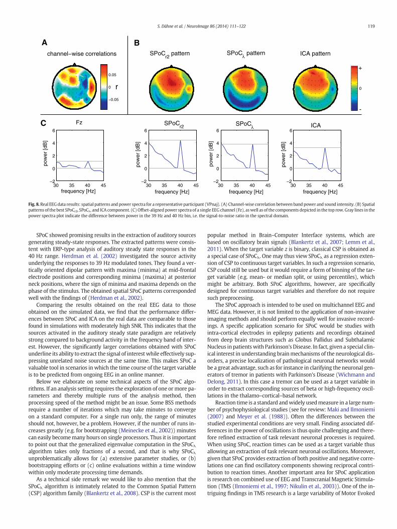
Fig. 8 shows more detailed results for a representative participant(VPnaj). These plots show channel-wise correlations plotted as a scalpmap; the spatial patterns of highest correlating SPoCr2, SPoCλ, and ICAcomponents; as well as the power spectra of a single EEG channel (Fz)and the spectra obtained after spatial filtering with the correspondingSPoCr2, SPoCλ, or ICA filter. Please note that for all subjects the SPoCλ fil-ter that maximized the covariance (i.e. the objective function of SPoCλ)also exhibited the maximal correlation between the power time courseand stimulus intensity. It can be seen that the channel-wise correlationsare low in magnitude and that the pattern of correlation values showslittle resemblancewith the components obtained from the spatial filter-ingmethods. Between SPoCr2, SPoCλ, and ICA, the obtained patterns arequite similar, indicating that the same source (or set of sources) hasbeen extracted by the algorithms. The second row of plots in Fig. 8shows the offset-aligned power spectra of EEG channel Cz and the re-spective best SPoCr2, SPoCλ, and ICA components (corresponding tothe spatial patterns above). The spatial filtering methods show a muchclearer peak at the steady-state frequency compared to the individualrecording channel. The peak is most pronounced in the componentextracted by SPoCr2, thus yielding the highest signal-to-noise ratio forthis particular participant.
Discussion
We presented a novel approach for the extraction of oscillatorysources showing a comodulation of their power with the target func-tion, the latter being for instance reaction time, hit rate or somephysicalproperties of the sensory stimuli (e.g. intensity). The SPoC approach isthe first to explicitly address the problem of component extraction forband power correlation/covariance. Using two implementations of ourapproach (the SPoCλ and the SPoCr2 algorithm) we were able to showthat it performed better than other methods commonly used for the in-vestigation of a relationship between behavioral measures and a powerof oscillations (sensor space regressions, ICA).
−0.05
0
0.05
channel−wise correlations SPoCr2
pattern SPoCλ pattern ICA pattern
Fz
frequency [Hz]
pow
er [d
B]
frequency [Hz] frequency [Hz] frequency [Hz]
ICASPoCλSPoC
r2
pow
er [d
B]
pow
er [d
B]
pow
er [d
B]
+
0
-
r
A
C
B
30 35 40 45−2
0
2
4
6
30 35 40 45−2
0
2
4
6
30 35 40 45−2
0
2
4
6
30 35 40 45−2
0
2
4
6
Fig. 8. Real EEGdata results: spatial patterns and power spectra for a representative participant (VPnaj). (A) Channel-wise correlation between band power and sound intensity. (B) Spatialpatterns of the best SPoCr2, SPoCλ, and ICA component. (C)Offset-aligned power spectra of a single EEG channel (Fz), aswell as of the components depicted in the top row. Gray lines in thepower spectra plot indicate the difference between power in the 39 Hz and 40 Hz bin, i.e. the signal-to-noise ratio in the spectral domain.
119S. Dähne et al. / NeuroImage 86 (2014) 111–122
SPoC showed promising results in the extraction of auditory sourcesgenerating steady-state responses. The extracted patterns were consis-tent with ERP-type analysis of auditory steady state responses in the40 Hz range. Herdman et al. (2002) investigated the source activityunderlying the responses to 39 Hz modulated tones. They found a ver-tically oriented dipolar pattern with maxima (minima) at mid-frontalelectrode positions and corresponding minima (maxima) at posteriorneck positions, where the sign of minima and maxima depends on thephase of the stimulus. The obtained spatial SPoC patterns correspondedwell with the findings of (Herdman et al., 2002).
Comparing the results obtained on the real EEG data to thoseobtained on the simulated data, we find that the performance differ-ences between SPoC and ICA on the real data are comparable to thosefound in simulations with moderately high SNR. This indicates that thesources activated in the auditory steady state paradigm are relativelystrong compared to background activity in the frequency band of inter-est. However, the significantly larger correlations obtained with SPoCunderline its ability to extract the signal of interest while effectively sup-pressing unrelated noise sources at the same time. This makes SPoC avaluable tool in scenarios in which the time course of the target variableis to be predicted from ongoing EEG in an online manner.
Below we elaborate on some technical aspects of the SPoC algo-rithms. If an analysis setting requires the exploration of one ormore pa-rameters and thereby multiple runs of the analysis method, thenprocessing speed of the method might be an issue. Some BSS methodsrequire a number of iterations which may take minutes to convergeon a standard computer. For a single run only, the range of minutesshould not, however, be a problem. However, if the number of runs in-creases greatly (e.g. for bootstrapping (Meinecke et al., 2002)) minutescan easily becomemany hours on single processors. Thus it is importantto point out that the generalized eigenvalue computation in the SPoCλalgorithm takes only fractions of a second, and that is why SPoCλunproblematically allows for (a) extensive parameter studies, or (b)bootstrapping efforts or (c) online evaluations within a time windowwithin only moderate processing time demands.
As a technical side remark we would like to also mention that theSPoCλ algorithm is intimately related to the Common Spatial Pattern(CSP) algorithm family (Blankertz et al., 2008). CSP is the current most
popular method in Brain–Computer Interface systems, which arebased on oscillatory brain signals (Blankertz et al., 2007; Lemm et al.,2011). When the target variable z is binary, classical CSP is obtained asa special case of SPoCλ. One may thus view SPoCλ as a regression exten-sion of CSP to continuous target variables. In such a regression scenario,CSP could still be used but it would require a form of binning of the tar-get variable (e.g. mean- or median split, or using percentiles), whichmight be arbitrary. Both SPoC algorithms, however, are specificallydesigned for continuous target variables and therefore do not requiresuch preprocessing.
The SPoC approach is intended to be used on multichannel EEG andMEG data. However, it is not limited to the application of non-invasiveimaging methods and should perform equally well for invasive record-ings. A specific application scenario for SPoC would be studies withintra-cortical electrodes in epilepsy patients and recordings obtainedfrom deep brain structures such as Globus Pallidus and SubthalamicNucleus in patientswith Parkinson's Disease. In fact, given a special clin-ical interest in understanding brainmechanisms of the neurological dis-orders, a precise localization of pathological neuronal networks wouldbe a great advantage, such as for instance in clarifying the neuronal gen-erators of tremor in patients with Parkinson's Disease (Wichmann andDelong, 2011). In this case a tremor can be used as a target variable inorder to extract corresponding sources of beta or high-frequency oscil-lations in the thalamo–cortical–basal network.
Reaction time is a standard andwidely usedmeasure in a large num-ber of psychophysiological studies (see for review: Maki and Ilmoniemi(2007) and Meyer et al. (1988)). Often the differences between thestudied experimental conditions are very small. Finding associated dif-ferences in the power of oscillations is thus quite challenging and there-fore refined extraction of task relevant neuronal processes is required.When using SPoC, reaction times can be used as a target variable thusallowing an extraction of task relevant neuronal oscillations. Moreover,given that SPoC provides extraction of both positive and negative corre-lations one can find oscillatory components showing reciprocal contri-bution to reaction times. Another important area for SPoC applicationis research on combined use of EEG and Transcranial Magnetic Stimula-tion (TMS (Ilmoniemi et al., 1997; Nikulin et al., 2003)). One of the in-triguing findings in TMS research is a large variability of Motor Evoked

120 S. Dähne et al. / NeuroImage 86 (2014) 111–122
Potentials (MEPs) produced by the stimulation of themotor cortex. Thisvariability in MEPs most likely reflects changes in cortical excitability,and thus analysis of pre-stimulus oscillatory activitymight allowuniqueopportunity to trace the nature of neuronal processes responsible forchanges in excitability. Previous research on this topic has primarilybeen performed in sensor space (Maki and Ilmoniemi, 2010; Sausenget al., 2009), where a mixture of multiple sources was a major draw-back. The use of SPoC would allow extraction of specific oscillatorysources associatedwith the changes in cortical excitability. Another sce-nariowhere SPoC can be used is for studying cortico-muscular rhythmicinteractions. They are usually studied with phase synchronization mea-sures (so called cortico-muscular coherence (Baker, 2007)). However, itbecomes increasingly clear that not only phase-to-phase but alsoamplitude-to-amplitude neuronal interactions (Bayraktaroglu et al.,2013; Daffertshofer and vanWijk, 2011) are important for understand-ing brain functioning. The use of SPoC would allow studying neuronalsources showing amplitude-to-amplitude interactions, which is indica-tive of interactions between local dynamics in the cortex and spinal cord(Bayraktaroglu et al., 2013).
The ability to gain understanding about the results of a parameteroptimization is an important aspect of machine learning methods(Montavon et al., 2013). Note that SPoC properly implements the com-monly accepted generative model of EEG/MEG and therefore it is possi-ble to meaningfully interpret its results within this generative model.This also allows subsequent source localization (Baillet et al., 2001;Haufe et al., 2008, 2011) or further multimodal processing (Bießmannet al., 2011; Fazli et al., 2012) — aspects that we will pursue in a futureresearch effort towards a better understanding of cognitive brainfunction.
In summary, SPoC is an approach that enables a reliable and fast ex-traction of neuronal oscillations,whose power time course comodulateswith an external target function. Because of SPoC's superiority to otherstandard techniques, we advocate its use for recovering associations be-tween cognitive/motor variables and neuronal activity.
Acknowledgments
SD, JH, and MT acknowledge funding by the European ICTProgramme Project FP7-224631 (TOBI). SD is also supported by GRK1589/1. FCM gratefully acknowledges support by the German Ministryof Education and Research (BMBF) through the ‘Adaptive BCI’ Project,FKZ 01GQ1115. SH acknowledges support by the BMBF Grant No.01GQ0850. KRM acknowledges funding by the World Class UniversityProgram through the National Research Foundation of Korea fundedby the Ministry of Education, Science, and Technology, under grantR31-10008. VNacknowledges fundingby theGermanResearch Founda-tion (DFG) grant no. KFO 247 and by the Bernstein Center for Computa-tional Neuroscience, Berlin.
Appendix A. Correlating the power of single sensors
Let us for simplicity assume that s is the only source whose power iscorrelated to the target, and there is only one noise source n, whosepower is not correlated to the target. The measurement at electrode kis then expressed as xk(t) = aks(t) + bkn, where ak and bk are the re-spective mixing coefficients. The band power at xk is given as the vari-ance over time, which simplifies as
Var xk tð Þ½ � ¼ a2kVar s tð Þ½ � þ b2kVar n tð Þ½ �¼ a2k þ b2k
due to the uncorrelatedness and unit variance properties of s and n. Letus now assume the data has been divided up into (subsequent) epochs,and the strengths of the signal and noise sources depend on the epoch.In the following we will adopt the convention that Var[⋅], Cov[⋅],and Corr[⋅] will be evaluated across the index of their arguments, e.g.
Var[g(t)] is the variance of some function g across the time index t andCov[g(e), f(e)] is the covariance of two functions f and g across epochs.Let Var[xk(t)](e) denote the variance of xk(t) in the epoch with indexe, thus making Var[xk](e) a function of e. The correlation between z(e)and the band power at channel k across epochs is then given by
Corr Var xk tð Þ½ � eð Þ; z eð Þ½ �
¼Cov a2k eð Þ þ b2k eð Þ; z eð Þ
h iffiffiffiffiffiffiffiffiffiffiffiffiffiffiffiffiffiffiffiffiffiffiffiffiffiffiffiffiffiffiffiffiffiffiffiffiffiffiffiffiffiffiffiffiffiffiffiffiffiffiffiffiffiffiffiffiffiVar a2k eð Þ þ b2k eð Þ� �
Var z eð Þ½ �q :
ðA:1Þ
Without loss of generality we can assume that Var[z(e)] = 1. More-over, since the noise power bk
2(e) is neither correlated to the signalpower ak2(e) nor to the target z(e),
Corr Var xk tð Þ½ � eð Þ; z eð Þ½ �
¼Cov a2k eð Þ; z eð Þ
h iffiffiffiffiffiffiffiffiffiffiffiffiffiffiffiffiffiffiffiffiffiffiffiffiffiffiffiffiffiffiffiffiffiffiffiffiffiffiffiffiffiffiffiffiffiffiffiffiffiffiVar a2k eð Þ� �þ Var b2k eð Þ� �q
¼Cov a2k eð Þ; z eð Þ
h iffiffiffiffiffiffiffiffiffiffiffiffiffiffiffiffiffiffiffiffiffiffiffiVar a2k eð Þ� �q
�ffiffiffiffiffiffiffiffiffiffiffiffiffiffiffiffiffiffiffiffiffiffiffiVar a2k eð Þ� �q
ffiffiffiffiffiffiffiffiffiffiffiffiffiffiffiffiffiffiffiffiffiffiffiffiffiffiffiffiffiffiffiffiffiffiffiffiffiffiffiffiffiffiffiffiffiffiffiffiffiffiVar a2k eð Þ� �þ Var b2k eð Þ� �q
¼ 1qCorr a2k eð Þ; z eð Þ
h i;
ðA:2Þ
with
q ¼
ffiffiffiffiffiffiffiffiffiffiffiffiffiffiffiffiffiffiffiffiffiffiffiffiffiffiffiffiffiffiffiffi1þ
Var b2k eð Þh i
Var a2k eð Þ� �vuut
: ðA:3Þ
That is, the correlation between z and the band power at channel k isthe desired correlation between z and the band power of the signalsource s normalized by a factor q which depends on the ratio of theband power variation of the signal and noise sources (and hence also in-directly on the strength of the mixing coefficients ak
2(e) and bk2(e)).
Hence, only for zero noise contribution bk(e) = 0,∀e or for zero noisepower variation Var[bk2(e)] = 0 the desired correlation can be recov-ered. If both these quantities are nonzero, the correlation score will bediscounted by a factor which differs for each channel.
Appendix B. Simulated EEG
Simulated EEGdatawas createdusing the following steps. Firstly,wegenerated time courses of Nbg + 1 hypothetical band-limited EEGsources (1 target source and Nbg + 100 background sources). For illus-trative purposes we chose the α-band as the frequency band of interest,i.e. 8 to 12 Hz. The oscillatory signals were created individually byconstructing the amplitude and phase spectrum and then using inverseFourier transform to obtain the time-domain signal. In the amplitudespectrum, the coefficients of the alpha band were set to 1, whereasthe amplitudes of all other frequencies were set to zero. The phase spec-trumwas chosen randomly for each source time course. Once the time-domain signalswere constructed, their envelopeswere normalized to 1.Thereafter the signals were multiplied with an amplitude modulationfunction that consisted of low-pass filtered white noise (filter cut-offbelow 0.5 Hz). An offset was added such that the slow amplitude mod-ulation was always larger than zero. Squaring the amplitude modula-tion function of a source yields the power modulation of that source.This constitutes the EEG data in ‘source space’.
Physiologically plausible spatial patternswere generated via a realis-tic EEG forward model (Fonov et al., 2011; Nolte and Dassios, 2005).Specifically, we placed model neural sources (i.e. electrical dipoles,here with randomly chosen orientation) at randomly chosen locations

121S. Dähne et al. / NeuroImage 86 (2014) 111–122
in 3D voxel space and computed the resulting scalp projections, whichwe denotewith the vectorai∈RNx for the ith source, whereNx = 58 de-notes the number of simulated EEG channels. Using these scalp projec-tions, we separately constructed the sensor space representation of thetarget source (denoted by xt) and the sensor space representation ofbackground neural activity (denoted by xbg):
xt tð Þ ¼ a1st tð Þ
xbg tð Þ ¼XNbg
i¼1
aisi tð Þ:
Additionally we added Gaussian distributed noise (zero mean andunit variance), which is spatially as well as temporally uncorrelated.The noise vector is denoted by �(t). These three constituents (source sig-nal, background activity and sensor noise) were stored in respectivedata matrices (e.g. Xt = [xt(1), ⋯, xt(T)], where Xbg as well as X� are de-fined accordingly). Finally, the data matrices were combined accordingto the following parameterized equation
X ¼ γXtþ Xbgþ γ�
Xtk kFX�; ðB:1Þ
where ‖Xt‖F denotes the Frobenius norm of the matrix Xt. The parame-ters γ and γ� control the relative weightings of the signal constituents:γ� controls the strength of the sensor noise, while γ controls thestrength of the target source. The value of γ� was fixed to 0.1 for all sim-ulations and the value of γ was varied.
References
Baillet, S., Mosher, J.C.J., Leahy, R.M.R., 2001. Electromagnetic brain mapping. IEEE SignalProcess. Mag. 18, 14–30. http://dx.doi.org/10.1109/79.962275.
Baker, S.N., 2007. Oscillatory interactions between sensorimotor cortex and the periphery.Curr. Opin. Neurobiol. 17, 649–655.
Başar, E., Schürmann, M., Başar-Eroglu, C., Karakaş, S., 1997. Alpha oscillations in brainfunctioning: an integrative theory. Int. J. Psychophysiol. 26, 5–29.
Bauer, M., Oostenveld, R., Peeters, M., Fries, P., 2006. Tactile spatial attention enhancesgamma-band activity in somatosensory cortex and reduces low-frequency activityin parieto-occipital areas. J. Neurosci. 26, 490–501. http://dx.doi.org/10.1523/JNEUROSCI.5228-04.2006.
Bayraktaroglu, Z., von Carlowitz-Ghori, K., Curio, G., Nikulin, V.V., 2013. It is not all aboutphase: amplitude dynamics in corticomuscular interactions. NeuroImage 64,496–504.
Bießmann, F., Plis, S.M., Meinecke, F.C., Eichele, T., Müller, K.R., 2011. Analysis of multi-modal neuroimaging data. IEEE Rev. Biomed. Eng. 4, 26–58.
Blankertz, B., Dornhege, G., Krauledat, M., Müller, K.R., Curio, G., 2007. The non-invasiveBerlin brain–computer interface: fast acquisition of effective performance in untrainedsubjects. NeuroImage 37, 539–550. http://dx.doi.org/10.1016/j.neuroimage.2007.01.051.
Blankertz, B., Tomioka, R., Lemm, S., Kawanabe, M., Müller, K.R., 2008. Optimizingspatial filters for robust EEG single-trial analysis. IEEE Signal Process. Mag. 25,41–56. http://dx.doi.org/10.1109/MSP.2008.4408441.
Blankertz, B., Sannelli, C., Halder, S., Hammer, E.M., Kübler, A., Müller, K.R., Curio, G.,Dickhaus, T., 2010. Neurophysiological predictor of SMR-based BCI performance.NeuroImage 51, 1303–1309. http://dx.doi.org/10.1016/j.neuroimage.2010.03.022.
Blankertz, B., Lemm, S., Treder, M., Haufe, S., Müller, K.R., 2011. Single-trial analysisand classification of ERP components — a tutorial. NeuroImage 56, 814–825.http://dx.doi.org/10.1016/j.neuroimage.2010.06.048.
Brovelli, A., Lachaux, J.P., Kahane, P., Boussaoud, D., 2005. High gamma frequency oscilla-tory activity dissociates attention from intention in the human premotor cortex.NeuroImage 28, 154–164. http://dx.doi.org/10.1016/j.neuroimage.2005.05.045.
Buzsáki, G., Draguhn, A., 2004. Neuronal oscillations in cortical networks. Science(New York, N.Y.) 304, 1926–1929. http://dx.doi.org/10.1126/science.1099745.
Colgin, L.L., Denninger, T., Fyhn, M., Hafting, T., Bonnevie, T., Jensen, O., Moser,M.B., Moser,E.I., 2009. Frequency of gamma oscillations routes flow of information in the hippo-campus. Nature 462, 353–357. http://dx.doi.org/10.1038/nature08573.
Daffertshofer, A., van Wijk, B.C.M., 2011. On the influence of amplitude on the connectiv-ity between phases. Front. Neuroinform. 5, 6.
Darchia, N., Campbell, I., Tan, X., Feinberg, I., 2007. Kinetics of NREM delta EEG powerdensity across NREM periods depend on age and on delta-band designation. Sleep30, 71–79.
Debener, S., Herrmann, C.A.C.S., Kranczioch, C., Gembris, D., Engel, A.K., 2003. Top–downattentional processing enhances auditory evoked gamma band activity. NeuroReport14, 683–686. http://dx.doi.org/10.1097/01.wnr.0000064987.
Demanuele, C., Broyd, S.J., Sonuga-Barke, E.J.S., James, C., 2012. Neuronal oscillations in theEEG under varying cognitive load: a comparative study between slow waves andfaster oscillations. Clin. Neurophysiol. 124, 247–262.
Fazli, S., Mehnert, J., Steinbrink, J., Curio, G., Villringer, A., Müller, K.R., Blankertz, B., 2012.Enhanced performance by a hybrid NIRS–EEG brain computer interface. NeuroImage59, 519–529.
Fonov, V., Evans, A.C., Botteron, K., Almli, C.R., McKinstry, R.C., Collins, D.L., 2011. Unbiasedaverage age-appropriate atlases for pediatric studies. NeuroImage 54, 313–327.
Galambos, R., Makeig, S., Talmachoff, P.J., 1981. A 40-Hz auditory potential recorded fromthe human scalp. Proc. Natl. Acad. Sci. U. S. A. 78, 2643–2647.
Gevins, A., Leong, H., Du, R., Smith, M.E., Le, J., DuRousseau, D., Zhang, J., Libove, J., 1995.Towards measurement of brain function in operational environments. Biol. Psychol.40, 169–186.
Gonzalez Andino, S.L., Michel, C.M., Thut, G., Landis, T., Grave de Peralta, R., 2005. Predic-tion of response speed by anticipatory high-frequency (gamma band) oscillations inthe human brain. Hum. BrainMapp. 24, 50–58. http://dx.doi.org/10.1002/hbm.20056.
Grosse-Wentrup, M., Schölkopf, B., Hill, J., 2011. Causal influence of gamma oscillations onthe sensorimotor rhythm. NeuroImage 56, 837–842. http://dx.doi.org/10.1016/j.neuroimage.2010.04.265.
Haegens, S., Händel, B.F., Jensen, O., 2011a. Top–down controlled alpha band activity insomatosensory areas determines behavioral performance in a discrimination task.J. Neurosci. 31, 5197–5204. http://dx.doi.org/10.1523/JNEUROSCI.5199-10.2011.
Haegens, S., Nácher, V., Hernández, A., Luna, R., Jensen, O., Romo, R., 2011b. Beta oscillationsin the monkey sensorimotor network reflect somatosensory decision making. Proc.Natl. Acad. Sci. U. S. A. 108, 10708–10713. http://dx.doi.org/10.1073/pnas.1107297108.
Hari, R., Hämäläinen, M., Joutsiniemi, S.L., 1989. Neuromagnetic steady-state responses toauditory stimuli. J. Acoust. Soc. Am. 86, 1033–1039.
Haufe, S., Nikulin, V.V., Ziehe, A., Müller, K.R., Nolte, G., 2008. Combining sparsity and ro-tational invariance in EEG/MEG source reconstruction. NeuroImage 42, 726–738.
Haufe, S., Tomioka, R., Dickhaus, T., Sannelli, C., Blankertz, B., Nolte, G., Müller, K.R., 2011.Large-scale EEG/MEG source localization with spatial flexibility. NeuroImage 54,851–859. http://dx.doi.org/10.1016/j.neuroimage.2010.09.003.
Herdman, A.T., Lins, O., Van Roon, P., Stapells, D.R., Scherg, M., Picton, T.W., 2002. Intrace-rebral sources of human auditory steady-state responses. Brain Topogr. 15, 69–86.
Holm, A., Lukander, K., Korpela, J., Sallinen, M., Müller, K.M.I., 2009. Estimating brain loadfrom the EEG. Sci. World J. 9, 639–651. http://dx.doi.org/10.1100/tsw.2009.83.
Ilmoniemi, R.J., Virtanen, J., Ruohonen, J., Karhu, J., Aronen, H.J., Näätänen, R., Katila, T.,1997. Neuronal responses to magnetic stimulation reveal cortical reactivity and con-nectivity. Neuroreport 8, 3537–3540.
Jensen, O., Kaiser, J., Lachaux, J.P., 2007. Human gamma-frequency oscillations associatedwith attention and memory. Trends Neurosci. 30, 317–324. http://dx.doi.org/10.1016/j.tins.2007.05.001.
Jin, Y., OHalloran, J.P., Plon, L., Sandman, C.A., Potkin, S.G., 2006. Alpha EEEG predictsvisual teaction time. Int. J. Neurosci. 116, 1035–1044. http://dx.doi.org/10.1080/00207450600553232.
John, M.S., Dimitrijevic, A., Picton, T.W., 2003. Efficient stimuli for evoking auditorysteady-state responses. Ear Hear. 24, 406–423. http://dx.doi.org/10.1097/01.AUD.0000090442.37624.BE.
Kaiser, J., Hertrich, I., Ackermann, H., Lutzenberger, W., 2006. Gamma-band activity overearly sensory areas predicts detection of changes in audiovisual speech stimuli.NeuroImage 30, 1376–1382. http://dx.doi.org/10.1016/j.neuroimage.2005.10.042.
Klimesch, W., 1999. EEG alpha and theta oscillations reflect cognitive and memoryperformance: a review and analysis. Brain Res. Rev. 29, 169–195.
Klimesch, W., Doppelmayr, M., Russegger, H., Pachinger, T., Schwaiger, J., 1998. Inducedalpha band power changes in the human EEG and attention. Neurosci. Lett. 244,73–76.
Lemm, S., Blankertz, B., Dickhaus, T., Müller, K.R., 2011. Introduction to machine learningfor brain imaging. NeuroImage 56, 387–399. http://dx.doi.org/10.1016/j.neuroimage.2010.11.004.
Maeder, C.L., Sannelli, C., Haufe, S., Blankertz, B., 2012. Prestimulus sensorimotor rhythmsinfluence brain–computer interface classification performance. IEEE Trans. NeuralSyst. Rehabil. Eng. 20, 653–662.
Makeig, S., Jung, T.P., 1996. Tonic, phasic, and transient EEG correlates of auditory aware-ness in drowsiness. Cogn. Brain Res. 4, 15–25.
Maki, H., Ilmoniemi, R.J., 2007. What, when, where in the brain? Exploring mental chro-nometry with brain imaging and electrophysiology. Rev. Neurosci. 18, 159–171.
Maki, H., Ilmoniemi, R.J., 2010. The relationship between peripheral and early corticalactivation induced by transcranial magnetic stimulation. Neurosci. Lett. 478, 24–28.
Meinecke, F., Ziehe, A., Kawanabe, M., Müller, K.R., 2002. A resampling approach to estimatethe stability of one-dimensional or multidimensional independent components. IEEETrans. Biomed. Eng. 49, 1514–1525. http://dx.doi.org/10.1109/TBME.2002.805480.
Meyer, D.E., Osman, A.M., Irwin, D.E., Yantis, S., 1988. Modern mental chronometry. Biol.Psychol. 26, 3–67.
Montavon, G., Braun, M.L., Krueger, T., Müller, K.-R., 2013. Analyzing local structure inKernel-based learning: explanation, complexity and reliability assessment. Signal Pro-cessing Magazine, IEEE 30 (4), 62–74. http://dx.doi.org/10.1109/MSP.2013.2249294.
Nikulin, V.V., Kicic, D., Kähkönen, S., Ilmoniemi, R.J., 2003. Modulation of electroencepha-lographic responses to transcranial magnetic stimulation: evidence for changes incortical excitability related to movement. Eur. J. Neurosci. 18, 1206–1212.
Nolte, G., Dassios, G., 2005. Analytic expansion of the EEG lead field for realistic volumeconductors. Phys. Med. Biol. 50, 3807–3823.
Nunez, P.L., Srinivasan, R., 2006. Electric Fields of the Brain: The Neurophysics of EEG,vol. 35. Oxford University Press. http://dx.doi.org/10.1063/1.2915137.
Osipova, D., Takashima, A., Oostenveld, R., Fernández, G., Maris, E., Jensen, O., 2006. Thetaand gamma oscillations predict encoding and retrieval of declarative memory.J. Neurosci. 26, 7523–7531. http://dx.doi.org/10.1523/JNEUROSCI.1948-06.2006.

122 S. Dähne et al. / NeuroImage 86 (2014) 111–122
Parra, L.C., Spence, C.D., Gerson, A.D., Sajda, P., 2005. Recipes for the linear analysis of EEG.NeuroImage 28, 326–341. http://dx.doi.org/10.1016/j.neuroimage.2005.05.032.
Picton, T.W., John, M.S., Dimitrijevic, A., Purcell, D., 2003. Human auditory steady-state re-sponses. Int. J. Audiol. 42, 177–219.
Plourde, G., Stapells, D.R., Picton, T.W., 1991. The human auditory steady-state evokedpotentials. Acta Otolaryngol. 491, 153–160.
Rieder, M.K., Rahm, B., Williams, J.D., Kaiser, J., 2011. Human γ—band activity and behav-ior. Int. J. Psychophysiol. 79, 39–48. http://dx.doi.org/10.1016/j.ijpsycho.2010.08.010.
Rodriguez, R., Picton, T., Linden, D., Hamel, G., Laframboise, G., 1986. Human auditorysteady state responses: effects of intensity and frequency. Ear Hear. 7, 300–313.
Romei, V., Brodbeck, V., Michel, C., Amedi, A., Pascual-Leone, A., Thut, G., 2008. Spontane-ous fluctuations in posterior alpha-band EEG activity reflect variability in excitabilityof human visual areas. Cereb. Cortex 18, 2010–2018. http://dx.doi.org/10.1093/cercor/bhm229.
Sauseng, P., Klimesch, W., Gerloff, C., Hummel, F.C., 2009. Spontaneous locally restricted EEGalpha activity determines cortical excitability in the motor cortex. Neuropsychologia 47,284–288. http://dx.doi.org/10.1016/j.neuropsychologia.2008.07.021.
Tallon-Baudry, C., Bertrand, O., Hénaff, M.A., Isnard, J., Fischer, C., 2005. Attentionmodulatesgamma-band oscillations differently in the human lateral occipital cortex and fusiformgyrus. Cereb. Cortex 15, 654–662. http://dx.doi.org/10.1093/cercor/bhh167.
Thut, G., Nietzel, A., Brandt, S.A., Pascual-Leone, A., 2006. Alpha-band electroencephalo-graphic activity over occipital cortex indexes visuospatial attention bias and predictsvisual target detection. J. Neurosci. 26, 9494–9502. http://dx.doi.org/10.1523/JNEUROSCI.0875-06.2006.
Wichmann, T., Delong, M.R., 2011. Deep-brain stimulation for basal ganglia disorders.Basal Ganglia 1, 65–77. http://dx.doi.org/10.1016/j.baga.2011.05.001.
Womelsdorf, T., Fries, P., 2007. The role of neuronal synchronization in selective attention.Curr. Opin. Neurobiol. 17, 154–160. http://dx.doi.org/10.1016/j.conb.2007.02.002.