Solar Phys (2012) 280:321–333DOI 10.1007/s11207-012-9949-0

A DVA N C E S I N E U RO P E A N S O L A R P H Y S I C S

Spontaneous Formation of Magnetic FluxConcentrations in Stratified Turbulence

Koen Kemel · Axel Brandenburg · Nathan Kleeorin ·Dhrubaditya Mitra · Igor Rogachevskii

Received: 2 December 2011 / Accepted: 13 February 2012 / Published online: 20 March 2012© Springer Science+Business Media B.V. 2012

Abstract The negative effective magnetic pressure instability discovered recently in directnumerical simulations (DNSs) may play a crucial role in the formation of sunspots and ac-tive regions in the Sun and stars. This instability is caused by a negative contribution ofturbulence to the effective mean Lorentz force (the sum of turbulent and non-turbulent con-tributions) and results in the formation of large-scale inhomogeneous magnetic structuresfrom an initially uniform magnetic field. Earlier investigations of this instability in DNSsof stably stratified, externally forced, isothermal hydromagnetic turbulence in the regime oflarge plasma β are now extended into the regime of larger scale separation ratios where thenumber of turbulent eddies in the computational domain is about 30. Strong spontaneousformation of large-scale magnetic structures is seen even without performing any spatialaveraging. These structures encompass many turbulent eddies. The characteristic time ofthe instability is comparable to the turbulent diffusion time, L2/ηt, where ηt is the turbu-lent diffusivity and L is the scale of the domain. DNSs are used to confirm that the effec-tive magnetic pressure does indeed become negative for magnetic field strengths below theequipartition field. The dependence of the effective magnetic pressure on the field strengthis characterized by fit parameters that seem to show convergence for larger values of themagnetic Reynolds number.

Keywords Magnetohydrodynamics (MHD) · Sun: dynamo · Sunspots · Turbulence

Advances in European Solar PhysicsGuest Editors: Valery M. Nakariakov, Manolis K. Georgoulis, and Stefaan Poedts

K. Kemel · A. Brandenburg (�) · N. Kleeorin · D. Mitra · I. RogachevskiiNordita, AlbaNova University Center, Roslagstullsbacken 23, 10691 Stockholm, Swedene-mail: brandenb@nordita.org

K. Kemel · A. BrandenburgDepartment of Astronomy, Stockholm University, 10691 Stockholm, Sweden

N. Kleeorin · I. RogachevskiiDepartment of Mechanical Engineering, Ben-Gurion University of the Negev, POB 653,Beer-Sheva 84105, Israel

322 K. Kemel et al.

1. Introduction

The 11-year solar activity cycle manifests itself through a periodic variation of the sunspotnumber. Sunspots consist of vertical magnetic fields with a strength of up to 3 kG in theircenter (see, e.g., Parker, 1979; Ossendrijver, 2003). It is generally believed that these fieldsalso continue in a similarly concentrated fashion beneath the surface in the form of mag-netic flux tubes or fibers (Parker, 1982). It was thought that fibral magnetic fields constitutea lower energy state and might therefore be preferred (Parker, 1984). Tube-like magneticfields were frequently seen in hydromagnetic turbulence simulations (Nordlund et al., 1992;Brandenburg, Procaccia, and Segel, 1995; Brandenburg et al., 1996), yet those tubes weresimilar to the vortex tubes in hydrodynamic turbulence. Such vortex tubes have typical di-ameters comparable to the viscous length; similarly, the aforementioned magnetic tubes seenin simulations have a thickness comparable to the resistive length. However, for the Sun, theresulting tube thickness would be too small to be relevant for sunspots.

At the surface, strong magnetic flux concentrations also form in regions of strong flowconvergence, but the size of these regions is too small for sunspots, because sunspots areusually much bigger than a single granular convection cell. In fact, a typical sunspot canhave a diameter of some 30 pressure scale heights. The tremendous size of sunspots hastherefore been used as an argument that they do not form near the surface, but at muchgreater depths near the bottom of the convection zone. At the bottom of the convection zonethe convection cells are big enough and could in principle be responsible for producingmuch bigger flux concentrations. Magnetic flux tubes can also form through the action ofshear, as shown by various simulations (Cline, Brummell, and Cattaneo, 2003; Guerrero andKäpylä, 2011). However, again it is possible that the size of such flux structures is related tothe resistive scale and therefore too small. While shear is likely an important ingredient ofthe solar dynamo, it remains unclear whether the resulting magnetic tubes are really able toproduce sunspots as a result of their piercing through the solar surface and, more importantly,whether one should consider them as being tied to the deep shear layers of the Sun.

In this paper we discuss an alternative scenario in which sunspots are shallow phenomenathat are not anchored at the bottom of the convection zone. Various mechanisms have beendiscussed, but of particular interest here are mechanisms that are based on the suppression ofturbulence by magnetic fields. In the mechanism of Kitchatinov and Mazur (2000) it is thesuppression of the turbulent heat flux, while in the mechanism of Rogachevskii and Kleeorin(2007) it is the suppression of the turbulent hydromagnetic pressure. Both mechanisms leadto a linear large-scale instability in a stratified medium. However, these mechanisms may beof different importance in different layers.

In this study we focus mainly on the second mechanism, which has recently been studiedin direct numerical simulations (DNSs) as well as in mean-field calculations. This mecha-nism is called the negative effective magnetic pressure instability (NEMPI). It is a convectivetype instability that is similar to the interchange instability in plasmas (Tserkovnikov, 1960;Newcomb, 1961; Priest, 1982) and the magnetic buoyancy instability (Parker, 1966). How-ever, the free energy in interchange and magnetic buoyancy instabilities is due to the gravi-tational field, while in NEMPI it is provided by the small-scale turbulence. NEMPI is causedby the suppression of turbulent hydromagnetic pressure by the mean magnetic field. Whenthe hydrodynamic Reynolds number is larger than unity and the mean magnetic field isless than the equipartition field strength, the negative turbulent contribution to the meanLorentz force is large enough so that the effective mean magnetic pressure (the sum ofturbulent and non-turbulent contributions) becomes negative (Kleeorin, Rogachevskii, andRuzmaikin, 1989, 1990; Rogachevskii and Kleeorin, 2007). This is the main reason for the

Spontaneous Formation of Magnetic Flux Concentrations 323

excitation of the large-scale instability that results in the formation of large-scale inhomo-geneous magnetic structures.

The effect of the suppression of the turbulent heat flux has not yet been studied as ex-tensively as NEMPI. An exception is the work of Kitchatinov and Olemskoy (2006), whohave used the model of Kitchatinov and Mazur (2000) to study the decay of sunspots. More-over, there is now some evidence that the effects anticipated by Kitchatinov and Mazur(2000) may have already been in operation in various simulations of solar convection wherethe spontaneous formation of pores has been seen (Stein et al., 2011). Such pores are ofthe size of several granules, but one may hope that the step toward structures of the sizeof active regions is a quantitative one that is controlled by the amount of flux present.Another example is the large-eddy simulation of Kitiashvili et al. (2010), where an im-posed vertical large-scale magnetic field is concentrated into giant vortices. This result isreminiscent of that of Tao et al. (1998), who found a segregation into magnetized andnearly unmagnetized regions in stratified convection simulations. However, it has not yetbeen possible to obtain large-scale magnetic structures resembling sunspots, except in mod-els with a strong imposed magnetic flux tube structure at the bottom of the domain (see,e.g., Rempel, Schüssler, and Knölker, 2009; Rempel et al., 2009; Cheung et al., 2010;Rempel, 2011a, 2011b). Such simulations demonstrate quite clearly that many aspects ofsunspot formation are now well understood. However, the physics involved in these simu-lations must become part of a larger picture in which the need for manually imposed fluxconcentrations is relaxed by self-consistently modeling their formation. Whether such fluxconcentrations originate from the tachocline (e.g., Cally, Dikpati, and Gilman, 2003) or fromthe upper layers remains an open question (Brandenburg, 2005). Here we focus on the latterscenario, where both NEMPI and the suppression of convective heat flux have been dis-cussed.

In the rest of this paper, we focus on NEMPI, which was first found in mean-field calcula-tions of a stratified layer (Kleeorin, Mond, and Rogachevskii, 1996; Rogachevskii and Klee-orin, 2007; Brandenburg, Kleeorin, and Rogachevskii, 2010; Kemel et al., 2012). However,those results remained unconvincing until NEMPI was also discovered in DNS (Branden-burg et al., 2011, hereafter BKKMR). It is therefore most appropriate to begin our discussionwith the latter.

2. The Model

Following the earlier work of BKKMR, we solve the equations for the velocity U, the mag-netic vector potential A, and the density ρ,

ρDUDt

= −c2s ∇ρ + J × B + ρ(f + g) + ∇ · (2νρS), (1)

∂A∂t

= U × B + η∇2A, (2)

∂ρ

∂t= −∇ · ρU, (3)

where ν is the kinematic viscosity, η is the magnetic diffusivity due to Spitzer conductiv-ity of the plasma, B = B0 + ∇ × A is the magnetic field, B0 = (0,B0,0) is the imposeduniform field, J = ∇ × B/μ0 is the current density, μ0 is the vacuum permeability, andSij = 1

2 (∂iUj + ∂jUi) − 13δij∇ · U is the traceless rate of strain tensor. The forcing func-

tion f consists of random, white-in-time, non-polarized plane waves with a certain average

324 K. Kemel et al.

wavenumber kf. The forcing strength is such that the turbulent rms velocity is approximatelyindependent of z with urms = 〈u2〉1/2 ≈ 0.1cs. We consider a domain of size Lx × Ly × Lz

in Cartesian coordinates (x, y, z), with periodic boundary conditions in the x and y direc-tions and stress-free perfectly conducting boundaries at top and bottom (z = ±Lz/2). Thevolume-averaged density is therefore constant in time and equal to its initial value, ρ0 = 〈ρ〉.The gravitational acceleration g = (0,0,−g) is chosen such that k1Hρ = 1, which leads to adensity contrast between bottom and top of exp(2π) ≈ 535, where k1 = 2π/Lz is the lowestwavenumber in the domain and Hρ = c2

s /g is the density scale height. Thus Lz/Hρ = 2π ,so the domain extends in the vertical direction over approximately six scale heights.

Our simulations are characterized by the scale separation ratio, kf/k1, the fluid Reynoldsnumber Re ≡ urms/νkf, the magnetic Prandtl number PrM = ν/η, and the magnetic Reynoldsnumber ReM ≡ Re PrM. Following earlier work (Brandenburg et al., 2012), it is clear thatNEMPI is more effective for small values of PrM, so here we choose PrM = 0.5 and ReM

in the range 0.7 – 70. The magnetic field is expressed in units of the local equipartition fieldstrength, Beq = √

μ0ρurms, while B0 is specified in units of the volume-averaged value,Beq0 = √

μ0ρ0urms. Note that Beq(z) = Beq0√

ρ(z)/ρ0. In addition to visualizations of theactual magnetic field, we also monitor �By = By − B0, where By is an average over y anda certain time interval �t . Time is expressed in eddy turnover times, τto = (urmskf)

−1. Thisis the relevant adjustment time to the application of a magnetic field, for example. It is alsothe relevant time scale for small-scale dynamo action. For comparison, we also considerthe turbulent-diffusive time scale, τtd = (ηt0k

21)

−1, where ηt0 = urms/3kf is the estimatedturbulent magnetic diffusivity. This is the time scale relevant for mean-field phenomena suchas those discussed here. Another diagnostic quantity is the rms magnetic field in the Fouriermode of k = k1, referred to as B1, which is taken here as an average over 2 ≤ k1z ≤ 3, and isclose to the top at k1z = π (note that B1 does not include the imposed field B0 at k = 0). Wehave chosen this z range because it is the one where the instability appears first; therefore,it is best seen in that range.

The simulations are performed with the PENCIL CODE,1 which uses sixth-order explicitfinite differences in space and a third-order accurate time stepping method. We use numer-ical resolutions of 1283 and 2563 mesh points when Lx = Ly = Lz, and 1024 × 1282 whenLx = 8Ly = 8Lz. To capture mean-field effects on the slower turbulent-diffusive time scale,which is τtd/τto = 3k2

f /k21 times slower than the dynamical time scale, we perform simula-

tions for several thousand turnover times.

3. Results

In simulations, the clearest indication of a spontaneous flux concentration is seen when thescale separation ratio is large. In BKKMR, we only used kf/k1 = 15. Here we considercalculations where this ratio is twice as large. A useful diagnostic is the magnetic fieldaveraged along the direction of the imposed field, i.e., along the y direction. In particular,we shall be looking at the y component of the field, i.e., 〈�By〉y/Beq. To see the effect evenmore clearly, we perform an additional time average over about 100 turnover times. Thisaverage is then referred to as 〈�By〉yt . In Figure 1 we show 〈�By〉yt /Beq for kf/k1 = 30. Theother parameters are ReM = 18 and PrM = 0.5. An inhomogeneous magnetic structure formsfirst near the surface (at t/τtd = 0.79), but then the structure propagates downward. This is

1http://pencil-code.googlecode.com.

Spontaneous Formation of Magnetic Flux Concentrations 325

Figure 1 Visualizations of 〈�By 〉y(x, z, t) for different times. Time is indicated in turbulent–diffusivetimes, (ηt0k2

1)−1, corresponding to about 5000 turnover times, i.e., t = 5000/urmskf, and the dimensionsin the horizontal and vertical directions are in units of Hρ . ReM = 18 and PrM = 0.5.

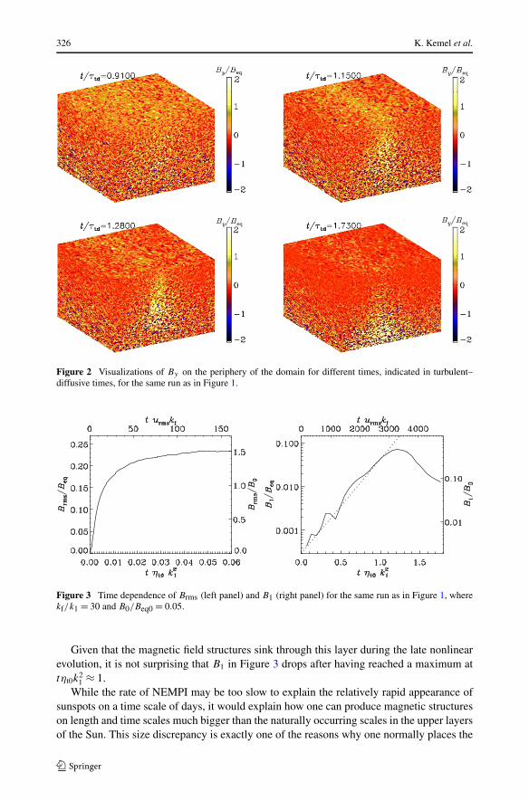
consistent with our interpretation that this is caused by negative effective magnetic pressureoperating on the scale of many turbulent eddies. Indeed, a local decrease of the effectivemagnetic pressure must be compensated by an increase in gas pressure, which implies higherdensity, so the structure becomes heavier and sinks in the nonlinear stage of NEMPI. Thisis also seen in three-dimensional visualizations without averaging; see Figure 2 with thesame parameters as in Figure 1. The top view of this figure justifies our assumption thatthe structures are two dimensional, and that averaging over the y direction was thereforemeaningful.

To confirm that NEMPI really is a large-scale instability, we would expect to see an ex-ponential growth phase. This is shown in the right-hand panel of Figure 3, where we showthe growth of B1 versus time. We recall that B1 measures the magnetic field variation nearthe top layer in 2 ≤ k1z ≤ 3; note that the equipartition field used for normalization is alsoaveraged over this layer. We give time both in turbulent-diffusive times (lower abscissa)as well as in eddy turnover times (upper abscissa). We do see that there is an exponen-tial growth phase which lasts for about one turbulent-diffusive time; i.e., the growth rate iscomparable to (ηt0k

2)−1, where ηt ≈ urms/3kf is the expected turbulent magnetic diffusivity(Sur, Brandenburg, and Subramanian, 2008). However, compared with the eddy turnovertime, (urmskf)

−1, the turbulent-diffusive time scale is 3(kf/k1)2 times slower. This illustrates

that NEMPI is indeed a very slow process compared with, for example, the saturation of theoverall rms magnetic field (left-hand panel of Figure 3).

326 K. Kemel et al.

Figure 2 Visualizations of By on the periphery of the domain for different times, indicated in turbulent–diffusive times, for the same run as in Figure 1.

Figure 3 Time dependence of Brms (left panel) and B1 (right panel) for the same run as in Figure 1, wherekf/k1 = 30 and B0/Beq0 = 0.05.

Given that the magnetic field structures sink through this layer during the late nonlinearevolution, it is not surprising that B1 in Figure 3 drops after having reached a maximum attηt0k

21 ≈ 1.

While the rate of NEMPI may be too slow to explain the relatively rapid appearance ofsunspots on a time scale of days, it would explain how one can produce magnetic structureson length and time scales much bigger than the naturally occurring scales in the upper layersof the Sun. This size discrepancy is exactly one of the reasons why one normally places the

Spontaneous Formation of Magnetic Flux Concentrations 327

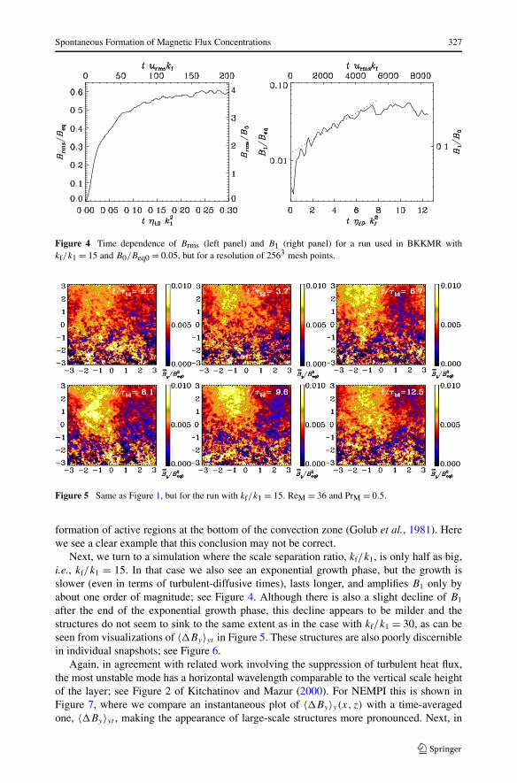
Figure 4 Time dependence of Brms (left panel) and B1 (right panel) for a run used in BKKMR withkf/k1 = 15 and B0/Beq0 = 0.05, but for a resolution of 2563 mesh points.

Figure 5 Same as Figure 1, but for the run with kf/k1 = 15. ReM = 36 and PrM = 0.5.

formation of active regions at the bottom of the convection zone (Golub et al., 1981). Herewe see a clear example that this conclusion may not be correct.

Next, we turn to a simulation where the scale separation ratio, kf/k1, is only half as big,i.e., kf/k1 = 15. In that case we also see an exponential growth phase, but the growth isslower (even in terms of turbulent-diffusive times), lasts longer, and amplifies B1 only byabout one order of magnitude; see Figure 4. Although there is also a slight decline of B1

after the end of the exponential growth phase, this decline appears to be milder and thestructures do not seem to sink to the same extent as in the case with kf/k1 = 30, as can beseen from visualizations of 〈�By〉yt in Figure 5. These structures are also poorly discerniblein individual snapshots; see Figure 6.

Again, in agreement with related work involving the suppression of turbulent heat flux,the most unstable mode has a horizontal wavelength comparable to the vertical scale heightof the layer; see Figure 2 of Kitchatinov and Mazur (2000). For NEMPI this is shown inFigure 7, where we compare an instantaneous plot of 〈�By〉y(x, z) with a time-averagedone, 〈�By〉yt , making the appearance of large-scale structures more pronounced. Next, in

328 K. Kemel et al.

Figure 6 Visualizations of By on the periphery of the domain for the run with kf/k1 = 15 and two timesthat are also shown in Figure 5. Note some slight enhancement of the field in the left part of the domain atlate times.

Figure 7 Visualization of By(x, z) for an elongated box (1024 × 1282 mesh points) with ReM = 36 ata time during the statistically steady state. The top panel shows the y average 〈�By 〉y/Beq at one timewhile the lower panel shows an additional time average 〈�By 〉yt /Beq covering about 80 turnover times. Thedimensions in the horizontal and vertical directions are Hρ , so the extent is 16πHρ × 2πHρ .

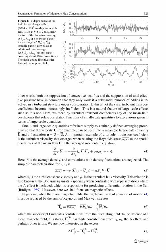
Figure 8 we compare cross sections of �By(x) (for fixed values of y, z, and t ; top panel)with corresponding y averages (middle panel) and yt averages (bottom panel). Here, ReM =36, kf/k1 = 15, and B0/Beq0 = 0.05. Without averaging, no clear magnetic structure is seenyet, but the structures become clearly more pronounced with y and t averaging. Runs withsimilar parameters have been shown in BKKMR for a computational domain whose x extentis 2π/k1 instead of 16π/k1.

The large-scale flux concentrations have an amplitude of only B1 ≈ 0.1Beq and are there-fore not easily seen in single snapshots, where the field reaches peak strengths compara-ble to Beq. Furthermore, as for any linear instability, the flux concentrations form a repeti-tive pattern, and are in that sense similar to flux concentrations seen in the calculations ofKitchatinov and Mazur (2000) that were based on the magnetic suppression of the turbulentheat flux. However, there are indications that, at larger values of ReM, flux concentrationsoccur more rarely, which might be more realistic in view of astrophysical applications.

4. Quantifying the Negative Effective Magnetic Pressure Effect

An important condition for the formation of structures by the mechanisms of Kitchatinovand Mazur (2000) and Rogachevskii and Kleeorin (2007) is sufficient scale separation. In

Spontaneous Formation of Magnetic Flux Concentrations 329

Figure 8 x dependence of thefield for an elongated box(1024 × 1282 mesh points) withReM = 36 at k1z = 2 (i.e., nearthe top of the domain) showing�By/Beq at y = 0 (top panel),its y average 〈�By 〉y/Beq(middle panel), as well as anadditional time average〈�By 〉yt /Beq (bottom panel)covering about 80 turnover times.The dash-dotted line gives thelevel of the imposed field.

other words, both the suppression of convective heat flux and the suppression of total effec-tive pressure have in common that they only work if a substantial number of eddies is in-volved in a turbulent structure under consideration. If this is not the case, turbulent transportcoefficients become increasingly inefficient. This is a natural feature of large-scale effectssuch as this one. Here, we mean by turbulent transport coefficients any of the mean-fieldcoefficients that relate correlation functions of small-scale quantities to expressions given interms of large-scale quantities.

Small- and large-scale quantities refer here simply to a suitably defined averaging proce-dure so that the velocity U, for example, can be split into a mean (or large-scale) quantityU and a fluctuation u = U − U. An important example of a turbulent transport coefficientis the turbulent viscosity that emerges when relating the Reynolds stress uiuj to the spatialderivatives of the mean flow U in the averaged momentum equation,

∂

∂tρ Ui = − ∂

∂xj

(ρ UiUj + ρ uiuj + · · ·). (4)

Here, ρ is the average density, and correlations with density fluctuations are neglected. Thesimplest parameterization for uiuj is

uiuj = −νt(Ui,j + Uj,i) − μtδij∇ · U, (5)

where νt is the turbulent shear viscosity and μt is the turbulent bulk viscosity. This relation isalso known as the Boussinesq ansatz, especially when contrasted with representations wherethe effect is included, which is responsible for producing differential rotation in the Sun(Rüdiger, 1989). However, here we shall focus on magnetic effects.

In general, when there are magnetic fields, the right-hand side of equation of motion (4)must be replaced by the sum of Reynolds and Maxwell stresses

�fij ≡ ρ uiuj − bibj /μ0 + 1

2b2/μ0, (6)

where the superscript f indicates contributions from the fluctuating field. In the absence of a

mean magnetic field, this stress, �f,0ij , has finite contributions from νt, μt, the effect, and

perhaps other terms. We are now interested in the excess,

��fij = �

f,Bij − �

f,0ij , (7)

330 K. Kemel et al.

that is caused solely by the presence of B. The only tensors that can be constructed with B

are those proportional to δij B2

and BiBj . This leads to the ansatz

��fij = qsBiBj/μ0 − 1

2qpδij B

2/μ0. (8)

Note in particular the definition of the signs of the terms involving the functions qs(B)

and qp(B). This becomes clear when writing down the mean Maxwell stress resulting fromboth mean and fluctuating fields, i.e.,

−BiBj/μ0 + 1

2δij B

2/μ0 + ��

fij = −(1 − qs)BiBj/μ0 + 1

2(1 − qp)δij B

2/μ0 + · · · (9)

Thus, the signs are defined such that for positive qs and qp the effects of magnetic stressand magnetic pressure are reduced and the signs of the net effects may even change.Equations (8) and (9) have been derived using the spectral τ relaxation approach (Klee-orin, Rogachevskii, and Ruzmaikin, 1990; Kleeorin, Mond, and Rogachevskii, 1996;Rogachevskii and Kleeorin, 2007) and the renormalization procedure (Kleeorin and Ro-gachevskii, 1994).

A broad range of different DNSs in stratified turbulence (Brandenburg et al., 2011, 2012)or turbulent convection (Käpylä et al., 2011) have now confirmed that qp is positive forReM > 1, but qs is small and perhaps even negative. A positive value of qs (but with largeerror bars) was originally reported for unstratified turbulence (Brandenburg, Kleeorin, andRogachevskii, 2010). Later, stratified simulations with isothermal stable stratification (Bran-denburg et al., 2012) and convectively unstable stratification (Käpylä et al., 2011) haveshown that it is small and negative. Nevertheless, qp(B) is consistently larger than unityprovided ReM > 1 while B/Beq is below a certain critical value that is around 0.5. This isshown in Figure 9, where we plot the effective magnetic pressure,

Peff(β) = 1

2

[1 − qp(β)

]β2 versus β ≡ |B|/Beq (10)

for different values of ReM using PrM = 0.5 and kf/k1 = 15. Note that the minimum ofPeff(β) is deeper for the case with ReM = 11 and then becomes shallower.

Note that βcrit is well below unity. This implies that it is probably not possible to pro-duce flux concentrations stronger than half the equipartition field strength. As such, mak-ing sunspots with this mechanism alone may be unlikely, and other effects such as that ofKitchatinov and Mazur (2000) may be needed. Such a mechanism would possibly work pref-erentially in the uppermost layers, provided that enough flux has already been accumulated.This may then be achieved with NEMPI, which also works in somewhat lower layers.

To compare the resulting functions Peff(β) in a systematic fashion for different parame-ters, we use the fit formula (Kemel et al., 2012)

qp(β) = qp0

1 + β2/β2p

= β2�

β2p + β2

, where β2� = qp0β2

p. (11)

To describe NEMPI accurately in a mean-field model, the fit should be good at low valuesof β. In Figure 9 we overplot fits where the parameters qp0 and βp have been determinedsuch that the minimum is well reproduced. However, note that then the fit becomes poor atlarger values of β, provided ReM 1.

The resulting dependencies βp(ReM), β�(ReM), and qp0(ReM) are shown in Figure 10 andcompared with the results of Brandenburg et al. (2012) for kf/k1 = 5. We see that β�(ReM)

varies relatively little between 0.1 and 0.2 and is typically around 0.15. For small values ofReM, βp(ReM) drops from 1 to 0.1 and then stays approximately constant, while qp0(ReM)

Spontaneous Formation of Magnetic Flux Concentrations 331

Figure 9 Normalized effectivemagnetic pressure, Peff(β), forlow (upper panel) and higher(lower panel) values of ReM. Thesolid lines represent the fits to thedata shown as dotted lines.

Figure 10 ReM dependence ofβp, β� , and qp0 for PrM = 0.5and kf/k1 = 15 (filled symbols)compared with those forkf/k1 = 5 (open red symbols) ofBrandenburg et al. (2012).

332 K. Kemel et al.

rises proportional to Re2M for ReM ≤ 10 and then levels off at a value around 40. The values

of βp and β� are slightly bigger for larger scale separation, while the values of qp0 are moresimilar.

The significance of a positive qs value comes from mean-field simulations with qs > 0 in-dicating the formation of three-dimensional (non-axisymmetric) flux concentrations (Bran-denburg, Kleeorin, and Rogachevskii, 2010). This result was later identified to be a directconsequence of having qs > 0 (Kemel et al., 2012). Before making any further conclusions,it is important to assess the effect of other terms that have been neglected. Two of them arerelated to the vertical stratification, i.e. additional terms in Equation (8) that are proportionalto gigj and giBj + gjBi with g being gravity. The coefficient of the former term seemsto be small (Käpylä et al., 2011), and the second only has an effect when there is a verti-cal or inclined imposed magnetic field. However, there could be other terms such as J iJ j

when the scale separation is not large enough. Furthermore, in astrophysically relevant sit-uations, the flow will possess helicity, so there can be pseudo-scalar coefficients in front ofpseudo-tensors such as J iBj and J jBi . Again, none of these effects is well explored yet.

5. Conclusions

In this paper we have performed detailed investigations of NEMPI detected recently byBKKMR. Most notably, we have extended the values of the scale separation ratio, kf/k1,from 15 to 30. In this case, the spontaneous formation of magnetic structures becomes par-ticularly evident and can be clearly noticed even without any averaging. Whether or not theparticular structures seen in DNS really have a correspondence to phenomena in the Suncannot be answered at the moment, because our model is still quite unrealistic in many re-spects. For example, in the Sun, kf and urms change with depth, which is not currently takeninto account in DNS. Also, of course, the stratification is not isothermal, but convectivelyunstable. However, DNSs in turbulent convection by Käpylä et al. (2011) have shown thatPeff(β) still has a negative minimum in that case, and it may even be deeper and wider thanin the isothermal case.

Regarding the production of sunspots, it is likely that NEMPI will shut off before themagnetic energy density has reached values comparable with the internal energy of the gas,as is the case in sunspots. Thus, some other mechanism is still needed to push the field of fluxconcentrations into that regime. One likely candidate is the mechanism of Kitchatinov andMazur (2000), where the suppression of convective heat flux by the magnetic field is crucial.This impression is further justified by recent calculations of Stein et al. (2011), where poresare seen to form spontaneously in a simulation where horizontal magnetic fields are injectedat the bottom of the domain.

Pores are small sunspots, with scales of a few granules, so something else is neededto make these structures bigger and to amplify this mechanism further. Again, the answercould be related to larger scale separation, which would allow NEMPI to operate and toconcentrate the magnetic field on scales encompassing many turbulent granules. Thus, eventhough NEMPI may not suffice to amplify fields to sunspot strengths, it would still be neededto produce active regions out of which sunspots grow by mechanisms such as convective fluxsuppression, as seen in models of Kitchatinov and Mazur (2000) and simulations of Steinet al. (2011). Thus, it is important to undertake detailed investigations of instabilities instrongly stratified layers with finite heat flux and finite magnetic field.

Spontaneous Formation of Magnetic Flux Concentrations 333

Acknowledgements We thank the anonymous referee for making detailed suggestions. We acknowledgethe NORDITA dynamo programs of 2009 and 2011 for providing a stimulating scientific atmosphere. Com-puting resources were provided by the Swedish National Allocations Committee at the Center for ParallelComputers at the Royal Institute of Technology in Stockholm and the High Performance Computing CenterNorth in Umeå. This work was supported in part by the European Research Council under the AstroDynResearch Project No. 227952.

References

Brandenburg, A.: 2005, Astrophys. J. 625, 539.Brandenburg, A., Procaccia, I., Segel, D.: 1995, Phys. Plasmas 2, 1148.Brandenburg, A., Kleeorin, N., Rogachevskii, I.: 2010, Astron. Nachr. 331, 5.Brandenburg, A., Jennings, R.L., Nordlund, Å., Rieutord, M., Stein, R.F., Tuominen, I.: 1996, J. Fluid Mech.

306, 325.Brandenburg, A., Kemel, K., Kleeorin, N., Mitra, D., Rogachevskii, I.: 2011, Astrophys. J. 740, L50

(BKKMR).Brandenburg, A., Kemel, K., Kleeorin, N., Rogachevskii, I.: 2012, Astrophys. J. doi:10.1088/0004-637X/

748/1/1. arXiv:1005.5700.Cally, P.S., Dikpati, M., Gilman, P.A.: 2003, Astrophys. J. 582, 1190.Cheung, M.C.M., Rempel, M., Title, A.M., Schüssler, M.: 2010, Astrophys. J. 720, 233.Cline, K.S., Brummell, N.H., Cattaneo, F.: 2003, Astrophys. J. 599, 1449.Golub, L., Rosner, R., Vaiana, G.S., Weiss, N.O.: 1981, Astrophys. J. 243, 309.Guerrero, G., Käpylä, P.J.: 2011, Astron. Astrophys. 533, A40.Käpylä, P.J., Brandenburg, A., Kleeorin, N., Mantere, M.J., Rogachevskii, I.: 2011, Mon. Not. Roy. Astron.

Soc. in press. arXiv:1105.5785.Kemel, K., Brandenburg, A., Kleeorin, N., Rogachevskii, I.: 2012, Astron. Nachr. 333, 95.Kitchatinov, L.L., Mazur, M.V.: 2000, Solar Phys. 191, 325.Kitchatinov, L.L., Olemskoy, S.V.: 2006, Astron. Lett. 32, 320.Kitiashvili, I.N., Kosovichev, A.G., Wray, A.A., Mansour, N.N.: 2010, Astrophys. J. 719, 307.Kleeorin, N., Rogachevskii, I.: 1994, Phys. Rev. E 50, 2716.Kleeorin, N.I., Rogachevskii, I.V., Ruzmaikin, A.A.: 1989, Sov. Astron. Lett. 15, 274.Kleeorin, N.I., Rogachevskii, I.V., Ruzmaikin, A.A.: 1990, Sov. Phys. JETP 70, 878.Kleeorin, N., Mond, M., Rogachevskii, I.: 1996, Astron. Astrophys. 307, 293.Newcomb, W.A.: 1961, Phys. Fluids 4, 391.Nordlund, Å., Brandenburg, A., Jennings, R.L., Rieutord, M., Ruokolainen, J., Stein, R.F., Tuominen, I.:

1992, Astrophys. J. 392, 647.Ossendrijver, M.: 2003, Astron. Astrophys. Rev. 11, 287.Parker, E.N.: 1966, Astrophys. J. 145, 811.Parker, E.N.: 1979, Cosmical Magnetic Fields, Oxford University Press, New York.Parker, E.N.: 1982, Astrophys. J. 256, 302.Parker, E.N.: 1984, Astrophys. J. 283, 343.Priest, E.R.: 1982, Solar Magnetohydrodynamics, Reidel, Dordrecht.Rempel, M.: 2011a, Astrophys. J. 729, 5.Rempel, M.: 2011b, Astrophys. J. 740, 15.Rempel, M., Schüssler, M., Knölker, M.: 2009, Astrophys. J. 691, 640.Rempel, M., Schüssler, M., Cameron, R.H., Knölker, M.: 2009, Science 325, 171.Rogachevskii, I., Kleeorin, N.: 2007, Phys. Rev. E 76, 056307.Rüdiger, G.: 1989, Differential Rotation and Stellar Convection: Sun and Solar-Type Stars, Gordon & Breach,

New York.Stein, R.F., Lagerfjärd, A., Nordlund, Å., Georgobiani, D.: 2011, Solar Phys. 268, 271.Sur, S., Brandenburg, A., Subramanian, K.: 2008, Mon. Not. Roy. Astron. Soc. 385, L15.Tao, L., Weiss, N.O., Brownjohn, D.P., Proctor, M.R.E.: 1998, Astrophys. J. 496, L39.Tserkovnikov, Y.A.: 1960, Sov. Phys. Dokl. 5, 87.