SPOT: Sliced Partial Optimal Transport · 2019-11-08 · SPOT: Sliced Partial Optimal Transport NICOLAS BONNEEL, Univ. Lyon, CNRS DAVID COEURJOLLY, Univ. Lyon, CNRS (a) Input (b)

SPOT: Sliced Partial Optimal Transport

NICOLAS BONNEEL, Univ. Lyon, CNRSDAVID COEURJOLLY, Univ. Lyon, CNRS

(a) Input (b) Target

(c) Full histogram matching (d) Partial histogram matching (e) Point clouds (f) Euclidean ICP (g) Our method

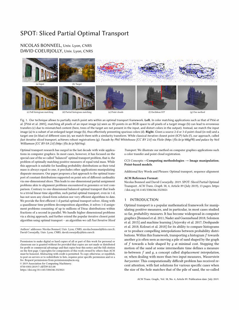
Fig. 1. Our technique allows to partially match point sets within an optimal transport framework. Left. In color matching applications such as that of Pitié etal. [Pitié et al. 2005], matching all pixels of an input image (a) seen as 3D points in an RGB space to all pixels of a target image (b) can lead to erroneoustransfers (c) due to mismatched content (here, trees of the target are not present in the input, and distort colors in the output). Instead, we match the inputimage (a) to a subset of an enlarged target image (b), thus effectively preventing spurious colors (d). Right. Given a source 2-d or 3-d point cloud (in red) and atarget one (in blue) of different sizes (e), we match them with a similarity transform. While classical iterative closest point (ICP) fails (f), our approach, calledfast iterative sliced transport, achieves robust registrations (g). Facade by Phil Whitehouse [CC BY 2.0] via Flickr (http://flic.kr/p/48kgPR) and palace by NeilWilliamson [CC BY-SA 2.0] (http://flic.kr/p/NJ6Vxq).

Optimal transport research has surged in the last decade with wide applica-tions in computer graphics. In most cases, however, it has focused on thespecial case of the so-called “balanced” optimal transport problem, that is, theproblem of optimally matching positive measures of equal total mass. Whilethis approach is suitable for handling probability distributions as their totalmass is always equal to one, it precludes other applications manipulatingdisparate measures. Our paper proposes a fast approach to the optimal trans-port of constant distributions supported on point sets of different cardinalityvia one-dimensional slices. This leads to one-dimensional partial assignmentproblems akin to alignment problems encountered in genomics or text com-parison. Contrary to one-dimensional balanced optimal transport that leadsto a trivial linear-time algorithm, such partial optimal transport, even in 1-d,has not seen any closed-form solution nor very efficient algorithms to date.We provide the first efficient 1-d partial optimal transport solver. Along witha quasilinear time problem decomposition algorithm, it solves 1-d assign-ment problems consisting of up to millions of Dirac distributions withinfractions of a second in parallel. We handle higher dimensional problemsvia a slicing approach, and further extend the popular iterative closest pointalgorithm using optimal transport – an algorithm we call Fast Iterative Sliced

Authors’ addresses: Nicolas Bonneel, Univ. Lyon, CNRS, [email protected];David Coeurjolly, Univ. Lyon, CNRS, [email protected].

Permission to make digital or hard copies of all or part of this work for personal orclassroom use is granted without fee provided that copies are not made or distributedfor profit or commercial advantage and that copies bear this notice and the full citationon the first page. Copyrights for components of this work owned by others than ACMmust be honored. Abstracting with credit is permitted. To copy otherwise, or republish,to post on servers or to redistribute to lists, requires prior specific permission and/or afee. Request permissions from [email protected].© 2019 Association for Computing Machinery.0730-0301/2019/7-ART89 $15.00https://doi.org/10.1145/3306346.3323021

Transport. We illustrate our method on computer graphics applications sucha color transfer and point cloud registration.

CCS Concepts: • Computing methodologies → Image manipulation;Point-based models.

Additional Key Words and Phrases: Optimal transport, sequence alignment

ACM Reference Format:Nicolas Bonneel and David Coeurjolly. 2019. SPOT: Sliced Partial OptimalTransport. ACM Trans. Graph. 38, 4, Article 89 (July 2019), 13 pages. https://doi.org/10.1145/3306346.3323021

1 INTRODUCTIONOptimal transport is a popular mathematical framework for manip-ulating positive measures, and in particular, in most cases studiedso far, probability measures. It has become widespread in computergraphics [Bonneel et al. 2011; Nader and Guennebaud 2018; Solomonet al. 2015] and machine learning [Arjovsky et al. 2017; Deshpandeet al. 2018; Kolouri et al. 2018] for its ability to compare histogramsor to produce compelling interpolations between probability distri-butions. Within this framework, transporting a histogram f towardsanother д is often seen as moving a pile of sand shaped by the graphof f towards a hole shaped by д at minimal cost. Stopping themotion of the sand at some intermediate time defines a measurein-between f and д, a concept called displacement interpolation,or, when dealing with more than two input measures,Wassersteinbarycenter. This computationally difficult problem has received re-cent attention, with fast solutions for various specific cases whenthe size of the hole matches that of the pile of sand, the so-called

ACM Trans. Graph., Vol. 38, No. 4, Article 89. Publication date: July 2019.

http://flic.kr/p/48kgPR

http://flic.kr/p/NJ6Vxq

https://doi.org/10.1145/3306346.3323021

https://doi.org/10.1145/3306346.3323021

https://doi.org/10.1145/3306346.3323021

89:2 • Bonneel et al.

balanced optimal transport problem [Bonneel et al. 2015; Kitagawaet al. 2016; Nader and Guennebaud 2018; Solomon et al. 2015].In our paper, we focus on discrete distributions with uniform

weights, that is, measures of the form∑xi δxi , i.e., a uniformly

weighted point cloud. In that form, the optimal transport problembetween these two measures is also known as a linear assignmentproblem. However, in contrast to most approaches, we do not assumeequal total masses, thus allowing for the hole to be larger than themass it receives. This scenario for instance occurs when one triesto match a 3-d point cloud within a larger point set, or when onetries to transfer colors between images of different sizes, in whichcase the assignment is only partial.Among existing solutions, for large datasets possibly involving

millions of points scattered in high dimension, the only tractable(balanced) optimal transport algorithm to date relies on a slicedapproximation [Bonneel et al. 2015; Pitié et al. 2005; Rabin et al.2011]. Slicing consists in projecting the point cloud onto random one-dimensional lines, and solving one-dimensional transport problems.The speed of this approach relies on the triviality of solving balancedone-dimensional transport problems. But surprisingly, even in 1-d,the partial optimal transport problem has received little attention,making this sliced approach unusable for point clouds of differentsizes.

Drawing connections between partial 1-d optimal transport andsequence alignment problems, we design a first solution of qua-dratic time complexity and linear space complexity outperformingstate-of-the-art dynamic programming solvers such as those usedin genomics. We further propose a new provably correct decom-position technique based on the number of non-injective nearestneighbor matches within quasilinear time complexity. This makesour algorithm efficient, even for problems involving millions ofpoint masses, and with each independent sub-problems solvable inparallel. We integrate this 1-d solver within a sliced optimal trans-port framework to handle higher dimensional point sets. We furtheradapt the popular Iterative Closest Point (ICP) algorithm to replacenearest neighbor’s matches by our sliced partial transport matches.We finally demonstrate applications such as proportion aware colortransfer between images, and point set registration. We summarizeour contributions as follows:• We introduce a fast 1-d exact partial optimal transport al-gorithm that solves problems involving millions on pointswithin fractions of a second. Its speed enables its use within asliced transport framework to manipulate higher dimensionaldistributions.• We develop a variant of the popular iterative closest pointpoint set registration algorithm using sliced partial optimaltransport that is more reliable on poorly initialized pointclouds.

2 PRIOR WORKOptimal transport is a computationally complex problem, oftenexpressed as a linear program due to Kantorovich (Table 1, (a)),and we refer the reader to recent books on the subject for detailson this theory [Peyré et al. 2017; Santambrogio 2015; Villani 2003].The variables being optimized form what is known as a transport

plan to describe the amount of mass from each bin of an input(possibly high-dimensional) histogram that needs to travel to eachbin of a target histogram. In this definition, it is assumed that bothhistograms are normalized. Directly solving this linear program canbe very costly, and has only been typically done for histograms ofup to a few tens of thousands of bins [Bonneel et al. 2011]. Fasteralternate approaches have tried to tackle particular cases, such assemi-discrete formulations [Gu et al. 2013; Kitagawa et al. 2016; Lévy2015; Mérigot 2011] for matching weighted point sets to continuousdensities via geometric constructions, or formulations to match 2-dcontinuous distributions to uniform continuous distributions [Naderand Guennebaud 2018]. Other approaches approximate the problem,such as entropy-regularized optimal transport, which results inblurred transport plan but is extremely fast to compute, especiallywhen data lie on a grid [Solomon et al. 2015]. However, when datado not lie on a grid, this method may require explicitly storing costmatrices between all pairs of bins thus making it intractable formore than a few tens of thousands of bins. As a last resort, slicedoptimal transport [Bonneel et al. 2015; Pitié et al. 2005; Rabin et al.2011] relies on random 1-d projections for which optimal transportis trivial, but comes at the cost of being optimal only on theseprojections and not necessarily on the higher dimensional space.The bulk of the computations lies within the sorting of projectedpoints on the line, which comes at an O(n logn) complexity.When histograms are not normalized, the transport problem

needs to be relaxed. Notably, the “unbalanced” optimal transport ofBenamou et al. [Benamou 2003] replaces hard constraints by softconstraints in a Monge formulation to accommodate for densities ofunequal masses within a PDE framework. Chizat et al. proposed afast numerical solution of the unbalanced problem [2016] in the caseof entropy-regularized optimal transport with soft constraints onmarginals, but suffering from the same space complexity as the bal-anced problem for scattered data. Figalli introduces partial optimaltransport that keeps all constraints of the linear program hard [Fi-galli 2010], but replaces equality with inequality constraints (Table 1,(b)). Our formulation is a special case of this linear program for theproblem of matching point clouds (Table 1, (c)).Our particular case specializes the above problem by Figalli in

four ways. First, we consider a simpler 1-d problem and only move tohigher dimensions via a slicing scheme. Second, we do not considergeneral functions or histograms, but only unweighted sets of Diracs;in the notations of Table 1, this amounts to f0(xi ) = 1 for xi ∈ X andf1(yj ) = 1 for yj ∈ Y where X and Y are two one-dimensional pointsets respectively of sizem andn. Third, we typically consider the costof moving a point from one place to another as being a quadratic cost,that is, c(x ,y) = (x − y)2 (note that we could consider any convexfunction of the distance without changing the assignment [Villani2003]). Finally, we require all the mass from the first, smaller, pointcloud to be matched to some parts of the target point cloud – in thenotations of Table 1, η = min(

∑f0,

∑f1) =m.

While at the surface this problem seems overly specific, it simplyamounts to matching point clouds of different cardinality, a commonproblem in computer graphics as we shall see in Sec. 6. Stated as anassignment problem, this question has been tackled as the linearassignment problem when point clouds have the same size [Lu andBoutilier 2015]. In a form related to the Monge optimal transport


SPOT: Sliced Partial Optimal Transport • 89:3

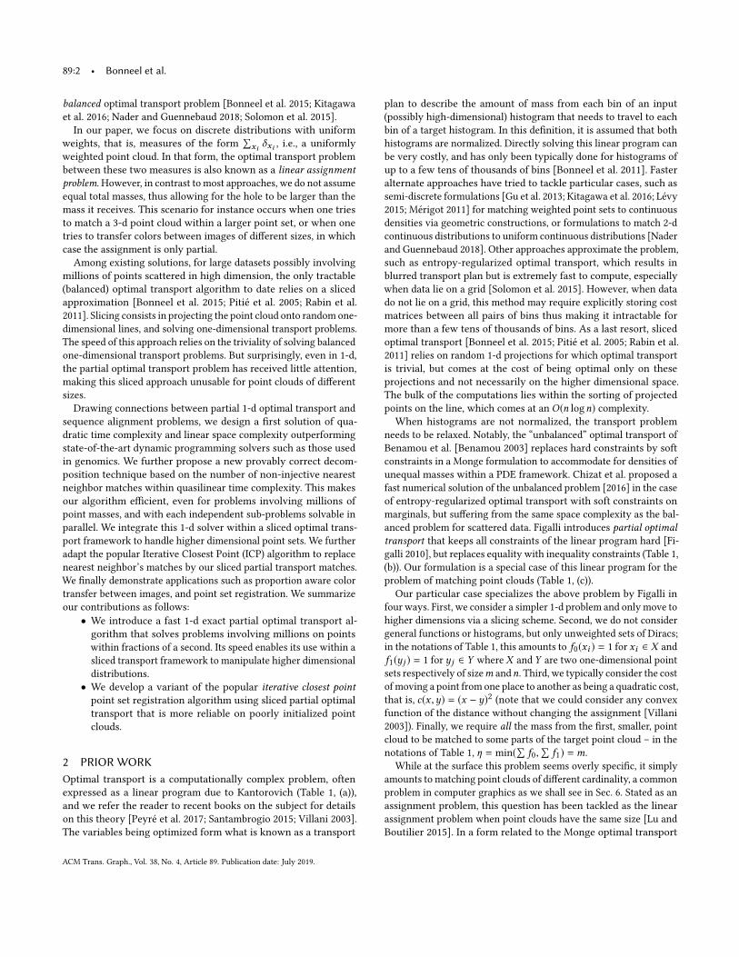
Table 1. We position our formulation (c) with respect to other optimal transport formulations. Formulation (a) assumes histograms are normalized andformalizes the classical optimal transport problem. Formulation (b) deals with histograms of different masses, only transporting a fraction η ≤ min(

∑f0,

∑f1).

Our formulation (c) is a linear assignment problem, and is a special case of (b) when η = min(∑f0,

∑f1) and when dealing with Dirac masses.

(a) Kantorovich discrete OT (b) Partial OT [Figalli 2010] (c) Linear Assignment (ours)

W (f0, f1) = minP

∑i, j

c(xi , yj )Pi, j (1)

s.t.Pi, j ≥ 0 , ∀i, j (2)m∑j=1

Pi, j = f0(xi ) , ∀i (3)

n∑i=1

Pi, j = f1(x j ) , ∀j (4)

Wp (f0, f1) =minP

∑i, j

c(xi , yj )Pi, j (5)

s.t. Pi, j ≥ 0 , ∀i, j (6)n∑j=1

Pi, j ≤ f0(xi ) , ∀i (7)

m∑i=1

Pi, j ≤ f1(x j ) , ∀j (8)

m∑i=1

n∑j=1

Pi, j = η (9)

Ws (f0, f1) = minP

∑i, j(xi − yj )2Pi, j

(10)s.t. Pi, j ≥ 0 , ∀i, j (11)

m∑j=1

Pi, j = 1 , ∀i (12)

n∑i=1

Pi, j ≤ 1 , ∀j (13)

formulation, this formulation amounts to finding an injective mapa : {1,m} ↪−→ {1,n} minimizing

mina injective

∑(xi − ya(i))

2 .

However, despite the simplicity of the problem formulation, suchassignment problems remain extremely difficult to solve, with evenapproximate state-of-the-art solutions taking hours to solve forlarge scale instances (millions of points) [Lu and Boutilier 2015] butusing more general cost functions.When restricting to 1-d domains and the class of cost functions

we target, the problem can be trivially solved ifm = n. In this case, itcan be shown that the trivial solution ends up pairing points in orderfrom left to right [Rabin et al. 2011]. Still in 1-d, whenm , n, theproblem can be solved by using a dynamic time warping algorithm,but this procedure is much more costly and, to our knowledge,has not been investigated for optimal transport. Such an algorithmmakes use of dynamic programming to find an alignment betweenthe two point sequences. This approach has been used in genomicsto align DNA sequences [Charter et al. 2000], for aligning textdocuments to display their “diff” [Gale andChurch 1991], to computethe Levenshtein distance between two strings [Levenshtein 1966], orto align audio sequences [Kaprykowsky and Rodet 2006]. A classicalexact algorithm is the Hirschberg’s algorithm [Hirschberg 1975],that, while only requiring O(m + n) storage (as opposed to O(mn)for standard dynamic programming), still performs in O(mn) timecomplexity and remains too slow in practice for large problems.

In contrast, while remaining in O(mn) in the worst case, we pro-vide an exact solution of large scale instances of millions of pointsin fractions of a second in 1-d, and approximately in seconds orminutes in n-d.

3 PARTIAL TRANSPORT IN 1-DGiven a set of points X = {xi ∈ R}i=1..m and Y = {yj ∈ R}i=1..non the real line,m < n, the goal is to find an injective assignmenta : {1,m} ↪−→ {1,n} minimizing

∑(xi − ya(i))

2.The core of our algorithm lies within an efficient 1-d assignment

procedure. It consists of a worst-case quadratic time complexitymatching that performs in near linear time in practice (Sec. 3.1),

and a problem decomposition that performs in quasilinear timecomplexity and allows each sub-problem to be solved independentlyin parallel (Sec. 3.3). Both rely on the same principles, and start witha (non injective) nearest neighbor assignment t .

3.1 Quadratic time algorithmWe first compute a nearest neighbor assignment t : {1,m} → {1,m}between X and Y . This can be performed in linear time by sortingboth sequences and scanning them at the same time from left toright since t(i + 1) ≥ t(i). The nearest neighbor match alreadyminimizes

∑(xi − yt (i))

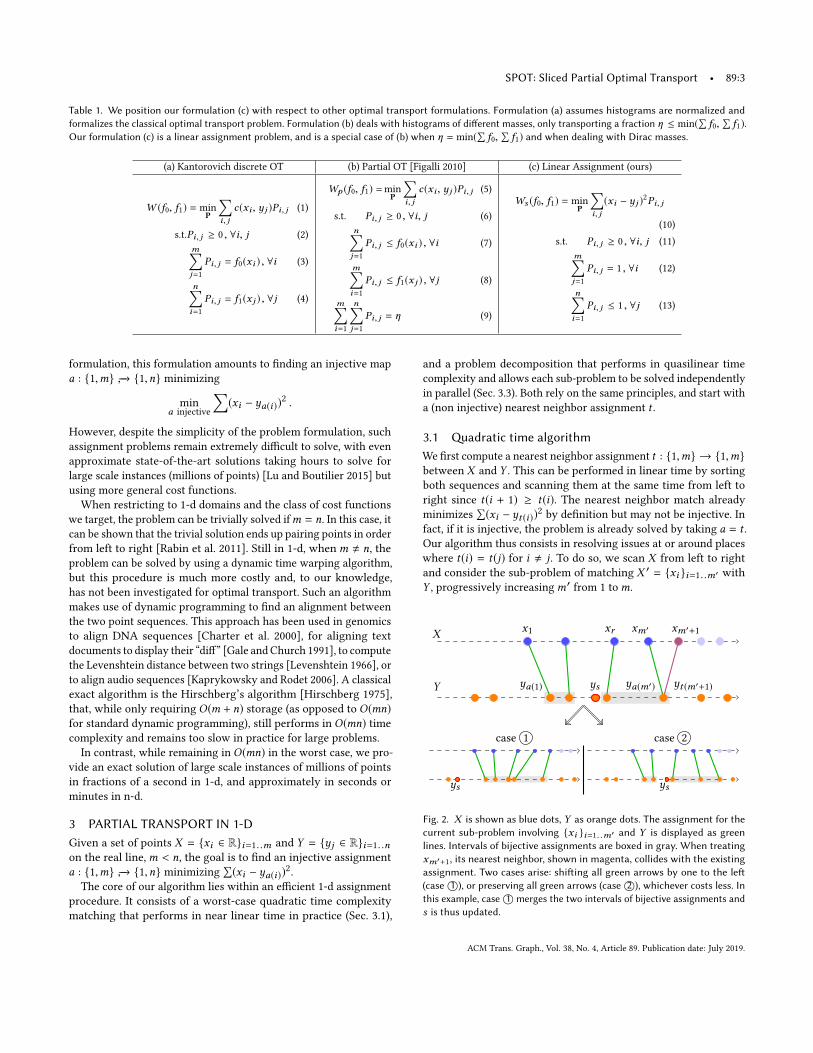
2 by definition but may not be injective. Infact, if it is injective, the problem is already solved by taking a = t .Our algorithm thus consists in resolving issues at or around placeswhere t(i) = t(j) for i , j. To do so, we scan X from left to rightand consider the sub-problem of matching X ′ = {xi }i=1..m′ withY , progressively increasingm′ from 1 tom.

X

Y ys

x1 xr

ya(1)

xm′ xm′+1

yt (m′+1)ya(m′)

ys

case 1

ys

case 2

Fig. 2. X is shown as blue dots, Y as orange dots. The assignment for thecurrent sub-problem involving {xi }i=1. .m′ and Y is displayed as greenlines. Intervals of bijective assignments are boxed in gray. When treatingxm′+1, its nearest neighbor, shown in magenta, collides with the existingassignment. Two cases arise: shifting all green arrows by one to the left(case 1○), or preserving all green arrows (case 2○), whichever costs less. Inthis example, case 1○ merges the two intervals of bijective assignments ands is thus updated.



Notations. Let us assume that we have solved the optimal as-signment problem of X ′ towards Y , denoted by a. The assignmentthus associates X ′ to the range of points {yj }j=a(1)...a(m′) ∈ Y (seeFig. 2). Such a range can be decomposed into intervals of consecu-tive points of Y which are each assigned to consecutive points ofX ′. We denote by s the rightmost point of {ya(1) . . .ya(m′)} whichis not assigned to any point of X ′. If the range has no such freespot s (in that case, a is bijective between X ′ and the range), we sets ← a(1) − 1. We denote by r the index of the point in X ′ such thata(r ) ← s + 11. By construction, a([r ,m′]) is a range of consecutiveinteger values [s + 1,a(m′)].Algorithm 1: Quadratic partial optimal assignment.input :Points X and Y .output :Optimal assignment of X to Y .

1 Let t be the nearest neighbor assignment of X to Y ;2 a(1) ← t(1);3 form′ from 2 tom do4 if t(m′ + 1) > a(m′) then5 a(m′ + 1) ← t(m′ + 1);6 else7 Retrieve s and r ;8 w1←

∑m′i=r (xi − ya(i)−1)

2 + (xm′+1 − ya(m′))2;

9 w2←∑m′i=r (xi − ya(i))

2 + (xm′+1 − ya(m′)+1)2;

10 if w1 < w2 then// case 1

11 a(m′ + 1) ← a(m′) + 1;12 a([r ,m′]) ← [s,a(m′) − 1];13 else

// case 2

14 a(m′ + 1) ← a(m′) + 1;

15 return {a(i)}i=1...m .

Update steps. We now consider the point xm′+1. If t(m′ + 1) >a(m′), we set a(m′+1) ← t(m′+1) – this corresponds to the nearestneighbor match t(m′) not colliding with any existing assignment.If t(m′ + 1) ≤ a(m′), we analyze two cases: case 1 offsets thelast subsequence of consecutive values in a to the left to leaveroom for a new assignment by setting a([r ,m′]) ← [s,a(m′) −1] and a(m′ + 1) ← a(m′) + 1. Case 2 directly pushes the newassignment on the right, that is, directly settinga(m′+1) ← a(m′)+1.To choose between these two cases, we compare their costs (w1and w2 in Algorithm 1) and proceed with the case with smallercost. Algorithm 1 describes this process. Its correctness is given inappendix. As we increasem′ tom during the update step, we endup with the optimal assignment of X to Y in O(max(n +m,m2)):the nearest neighbor assignment t is obtained in O(n +m). Then,for (possibly) eachm′ between 1 andm we evaluate two sums inO(m′ − r ). As we shall see in Sec. 3.4, we can considerably improvethe efficiency of the algorithm making it tractable for large scaleproblems (millions of points) by recursively updating these sums,only re-evaluating them occasionally.

1When a(1) = 1, s is undefined. In that case, we set r ← 1 and proceed with only case2 steps of our algorithm described next.

3.2 Simplifying the problemIn many cases, parts of the initial problem can be solved in lineartime. For instance, we can detect if t is injective in linear time, inwhich case the problem is solved by setting a ← t . Also, ifm = n, thetrivial assignment a([1,m]) ← [1,m] is optimal. We explain belowthree other cases that simplify or even solve the initial problem inlinear time.First, when there exists some k such that xi < y1 ,∀i < k , i.e., X

starts “before” Y , we can assign a(i) ← i ,∀i < k . This can be madeeven stronger: while xi < yi , we set a(i) ← i as illustrated below.

⇒

This holds symmetrically at the end of the sequence and often allowsto significantly reduce the problem range.Second, we can further reduce the range of Y based on the

number of non-injective values in the nearest neighbor map t .Specifically, let p = card{t(i) = t(i + 1), ∀i < m}. Then, itis enough to consider the sub-problem of matching X to Y ′ ={yj }j=max(1,t (1)−p)..min(t (m)+p,n):

⇒p = 3

A less tight bound, considering only the interval [max(1, t(1) −m),min(t(m) +m,n)] in Y , could be constructed in O(logn) with-out requiring any nearest neighbor computation. A proof of bothstatements is provided in supplementary material.Finally, whenm = n − 1, a linear time solution can be obtained,

inspired by Hirschberg’s algorithm [1975]. In this case, there ex-ists some k to be determined such that a([1,k − 1]) = [1,k − 1]and a([k,m]) = [k + 1,n]. Such k minimizes mink

∑k−1i=1 (xi −yi )

2 +∑mi=k (xi − yi+1)

2. Denoting C =∑mi=1(xi − yi+1)

2, the above mini-mization problem can bewrittenmink

∑ki=1(xi−yi )

2+C−(xi−yj+1)2

which can be obtainedwithin a single linear search, asC is a constantand need not be computed.

⇒ yk

All these simplification steps have a computational cost in O(m +n)and can be used as preprocessing to reduce X and Y before usingthe quadratic algorithm of Sec. 3.1.

3.3 Quasilinear time problem decompositionA key component of our algorithm is a quasilinear time decompo-sition, often allowing to decompose the initial problem into manysmall independent sub-problems that can be solved in parallel, andthat all benefit from simplifications exposed in Sec. 3.2.The bottleneck of our quadratic time solution is the need to re-

evaluate a possibly large sum many times during the run of thealgorithm to determine the better of two cases 1 or 2 . The keyintuition is that both cases can be kept as candidates without per-forming any summation. We maintain intervals of points in Y thatcontain both cases – these intervals may thus contain gaps, whichultimately will not be assigned by an point inX . The main advantage



X1 X2 X2

Y1 Y2 Y3

⇒A1 A2 A3

s1 ℓ1s2/s3

ℓ2/ℓ3

X ′1 X ′2

Y ′1 Y ′2

A′1 A′2s1 ℓ1/s2 ℓ2

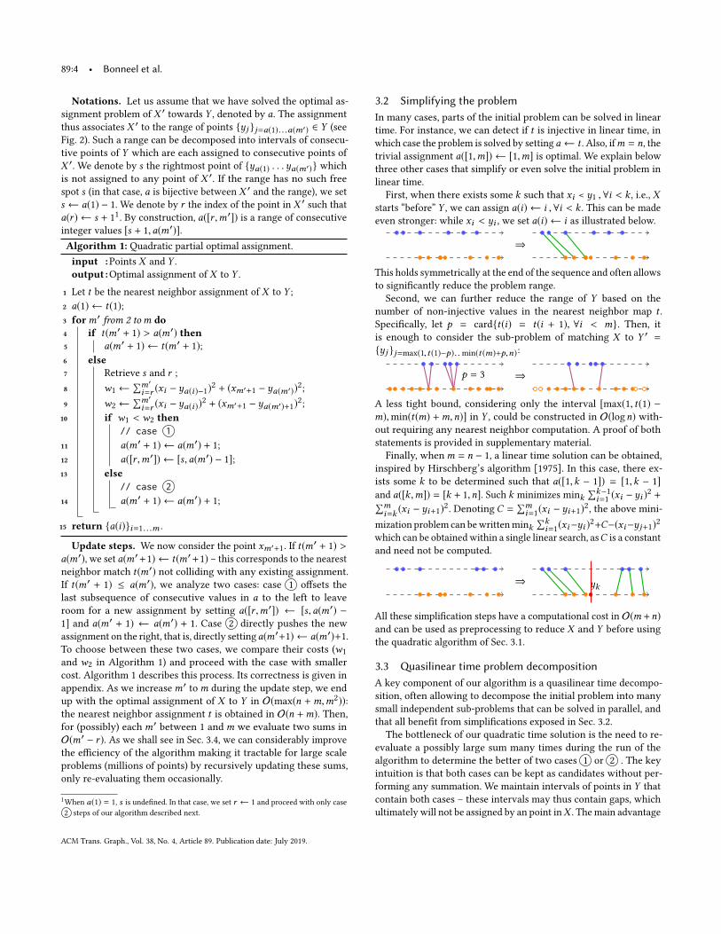
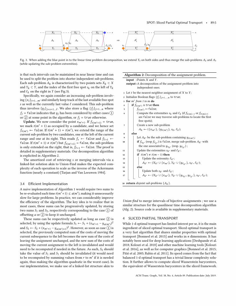
Fig. 3. When adding the blue point in to the linear time problem decomposition, we extend Y3 on both sides and thus merge the sub-problems A2 and A3(while updating the sub-problem extremities).

is that such intervals can be maintained in near linear time and canbe used to split the problem into shorter independent sub-problems.Each sub-problem Ak is characterized by two points sets Xk ⊂ Xand Yk ⊂ Y , and the index of the first free spot sk on the left of Ykand ℓk on the right in Y (see Fig.3).

Specifically, we again consider an increasing sub-problem involv-ing {xi }i=1..m′ and similarly keep track of the last available free spots as well as the currently last value ℓ considered. This sub-problemthus involves {yj }j=s+1..ℓ . We also store a flag { fj }j=1..n wherefj = false indicates that yj has been considered by either cases 1or 2 at some point in the algorithm, or fj = true otherwise.

Update. We now consider the point xm′+1. If ft (m′+1) = true,we mark t(m′ + 1) as occupied by a candidate, and we hence setft (m′) ← false. If t(m′ + 1) = t(m′), we extend the range of thecurrent sub-problem by two candidates, one at the left of the currentrange and one at its right. This reads fs ← false and fℓ+1 ←false. If t(m′ + 1) , t(m′) but ft (m′+1) = false, the sub-problemis only extended on the right, that is, fℓ+1 ← false. The proof isdetailed in supplementary materials. Our decomposition algorithmis explicited in Algorithm 2.The amortized cost of retrieving s or merging intervals via a

linked-list solution akin to Union-Find makes the expected com-plexity of each operation to scale as the inverse of the Ackermannfunction (nearly a constant) [Tarjan and Van Leeuwen 1984].

3.4 Efficient ImplementationA naive implementation of Algorithm 1 would require two sums tobe re-evaluated each time t(m′+1) ≤ a(m′), making it unnecessarilyslow for large problems. In practice, we can considerably improvethe efficiency of the algorithm. The key idea is to realize that inmost cases, these sums can be progressively updated, by storingtwo sums S1 and S2, respectively corresponding to the case 1 ofoffsetting a or 2 to keep it unchanged.These sums can be respectively updated as long as case 2 is

selected, by using the update formula S1 ← S1 + (xm′+1 − ya(m′))2

and S2 ← S2 + (xm′+1 − ya(m′)+1)2. However, as soon as case 1 is

selected, the previously computed sum of the costs of moving thecurrent subsequence to the left becomes the new sum of the costs ofleaving the assignment unchanged, and the new sum of the costs ofmoving the current assignment to the left is invalidated and wouldneed to be recomputed if needed in the future. As such, S2 shouldtake the value of S1 and S1 should be invalidated (it would needto be recomputed by summing values from r tom′ if it is neededagain, thus making the algorithm quadratic in the worst case). Inour implementation, we make use of a linked-list structure akin to

Algorithm 2: Decomposition of the assignment problem.input :Points X and Y .output :A decomposition of the assignment problem into

independent ones.

1 Let t be the nearest neighbor assignment of X to Y ;2 Initialize Boolean flags {fj }j=1. . .n to true;3 form′ from 1 tom do4 if ft (m′) is true then5 ft (m′) ←false;6 Compute the extremities sk and ℓk (if ft (m)−1 or ft (m)+1

are false we may traverse sub-problems to locate the firstfree spots);

7 Create a new sub-problemAk ← ({xm′ }, {yt (m′) }, sk , ℓk );

8 else9 Let Ak′ be the sub-problem containing yt (m′);

10 if fsk′ (resp fℓk′ ) is false, merge sub-problem Ak′ withthe one associated to ysk′ (resp. yℓk′ ) ;

11 Update the extremities sk′ and ℓk′ ;12 if t (m′) , t (m − 1) then13 Update the extremity ℓk′ ;14 Ak′ ← (Xk′ ∪ {xm′ }, Yk′ ∪ {yℓk′ }, sk′, ℓk′ );15 else16 Update both sk′ and ℓk′ ;17 Ak′ ← (Xk′ ∪ {xm′ }, Yk′ ∪ {ysk′ , yℓk′ }, sk′, ℓk′ );

18 return disjoint sub-problems {Ak }.

Union-find to merge intervals of bijective assignments ; we use asimilar structure for the quasilinear time decomposition algorithm(Alg. 2). Source code is available in supplementary materials.

4 SLICED PARTIAL TRANSPORTWhile 1-d optimal transport has limited interest per se, it is the mainingredient of sliced optimal transport. Sliced optimal transport isa very fast algorithm that shares similar properties with optimaltransport [Bonneel et al. 2015] and works in n dimensions. It hasnotably been used for deep learning applications [Deshpande et al.2018; Kolouri et al. 2018] and other machine learning tools [Kolouriet al. 2016], as well as for computer graphics [Bonneel et al. 2015;Pitié et al. 2005; Rabin et al. 2011]. Its speed comes from the fact thatbalanced 1-d optimal transport has a trivial linear complexity solu-tion. It further allows to compute sliced Wasserstein barycenters,the equivalent of Wasserstein barycenters in the sliced framework.



However, the balanced condition makes it difficult to use for prob-lems that are intrinsically unbalanced.Our partial 1-d optimal transport solution, while of quadratic

complexity in the worst case, is fast (see experiments in Sec. 6.4) andis thus amenable to the computation of sliced optimal transport. Also,formulas for gradients and Hessians computed for the balanced caseby Bonneel et al. [2015] remain unchanged in the partial transportcase. The algorithm for sliced (partial) Wasserstein barycenters issummarized below.

The sliced Wasserstein barycenter of a set of d-dimensional pointsets {Xk }k=1..K weighted by {λk }k=1..K is defined as theminimizer

argminX̃

E(X̃ ) = argminX̃

∑k

λk

∫Sd−1

WS (Projω (X̃ ), Projω (Xk ))dω ,

where Sd−1 is the (d − 1)-dimensional sphere of directions, usuallydiscretized over a finite set of directions Θ (uniformly or randomly),Projω (X ) projects the point set X onto the line of direction ω asProjω (X ) = {⟨xi ,ω⟩}i .W is the transport cost as computed in Sec. 3.Minimizing this energy can be performed via a gradient descentor Newton steps [Bonneel et al. 2015]. In fact, the gradient can beeasily expressed as:

∇E(X̃ ) =∑k

λk

∫Sd(Projω (X̃ ) − Projω (Xk ◦ ak )) ,

where ak is the assignment function of the (partial) optimal trans-port between X̃ and Xk . The Hessian is also easily computed inclosed form as

H (X̃ ) =1|Θ|

∑θ ∈Θ

θθ t ≈1dIdd×d ,

where θ t denotes the transpose of the direction θ . With these values,one can perform Newton’s iterations via the update X̃ ← X̃ −

H−1∇E(X̃ ). Transporting an entire point cloudX0 toX1 correspondsto a gradient descent ofW S (X0,X1). In this case, we resort to astochastic gradient descent strategy and perform descent steps witha single randomly determined direction at a time.

5 ITERATIVE TRANSPORT ALGORITHMA common problem in point cloud processing is that of register-ing points under a given transformation model. For instance, onetries to match a point cloud with another by supposing the trans-formation between them is rigid, or constrained to a similarity, oraffine, or homographic, etc. A well-known algorithm to solve thisproblem is the Iterative Closest Point (ICP) algorithm. Given a pointcloud X0 to be matched against X1, this algorithm proceeds by firstmatching points of X0 to their nearest neighbors in X1, and, giventhis assignment, the best transformation in the class of allowedtransformations is found by minimizing an energy (typically, forrigid or similarity transformations, the transformation can be foundvia an orthogonal Procrustes problem [Schönemann 1966] usingSingular Value Decompositions or Kabsch algorithm). The algo-rithm then transforms the initial point cloud using the computedtransformation. The process is repeated until convergence.However, this algorithm requires points clouds to be relatively

close to start with and suffers from local minima.While this has beenaddressed by Yang et al. [2013] for estimating rigid motion leading

to a globally optimal solution, this does not easily extend to otherclasses of transformations. In practice, we observe that extremelybad behaviors may arise when considering similarity transforms(rotation, translation and scaling). In that case, the lack of injectivityof the nearest neighbor map tends to estimate progressively smallerscaling factors as iterations increase, occasionally leading to a trivialzero scale solution: this solution is in fact globally optimal for theICP problem, leading to a zero cost of matching the entire inputpoint cloud to a single nearest neighbor point in the target pointcloud (see Fig. 9). This motivates the use of a metric which accountsfor an injective mapping, such as the sliced metric we are proposing.We thus propose to replace the nearest neighbor matching by

a partial sliced optimal transport matching. We call our algorithmFast Iterative Sliced Transport (FIST). We illustrate our results on 3dpoint cloud registration using a similarity transform in Sec. 6.2.

6 APPLICATIONS AND RESULTSThis section details two applications of our partial sliced optimaltransport framework. The first matches colors in a photograph bypossibly using superpixels, and the second uses our FIST algorithmto register point clouds. We then analyze our algorithm in term ofperformance.

6.1 Color MatchingTransferring colors between images has become a classical imageprocessing problem. The goal is to distort the color distribution ofan input image, without changing its content, to match the style ofa target image. This matching problem has seen numerous optimaltransport solutions [Bonneel et al. 2015, 2013; Pitié et al. 2005; Pitiéet al. 2007; Rabin et al. 2010]. In addition to their use of optimaltransport, a common point to these approaches is that they considerthe problem of matching normalized histograms. A consequenceof that is often acknowledged as a limitation: their content shouldnot differ. For instance, matching an image with 80% trees and 20%sky to an image containing the opposite ratio will inevitably leadto trees becoming blue or sky becoming green. This is illustratedin our teaser, Fig. 1, in which the input image does not contain thecolorful trees of the target image, thus leading to unatural colors inthe transferred example using the formulation of Pitié et al. [2005].Several approaches also require the images to have exactly the samenumber of pixels – this is precisely the case for sliced transporta-tion [Bonneel et al. 2015; Rabin et al. 2010].

To address this issue we propose two solutions within our SPOTframework. Our first solution simply enlarges the target images togive more freedom to each input pixel to be matched to target pixelvalues. Our second solution, inspired by that of Rabin et al. [2014] inthe context of relaxed optimal transport, segments the input imageinto a number of superpixels using the SLIC algorithm [Achantaet al. 2010] and consider the problem of matching each superpixelcolor distribution independently in the target image. To preventdiscontinuities between adjacent superpixels cares need to be taken.In particular, all superpixels should use the same set of projectiondirections, and we further apply the color transfer regularizationtechnique of Rabin et al. [Rabin et al. 2010] (altered to use a crossbilateral filter for simplicity [Paris and Durand 2009]). While the



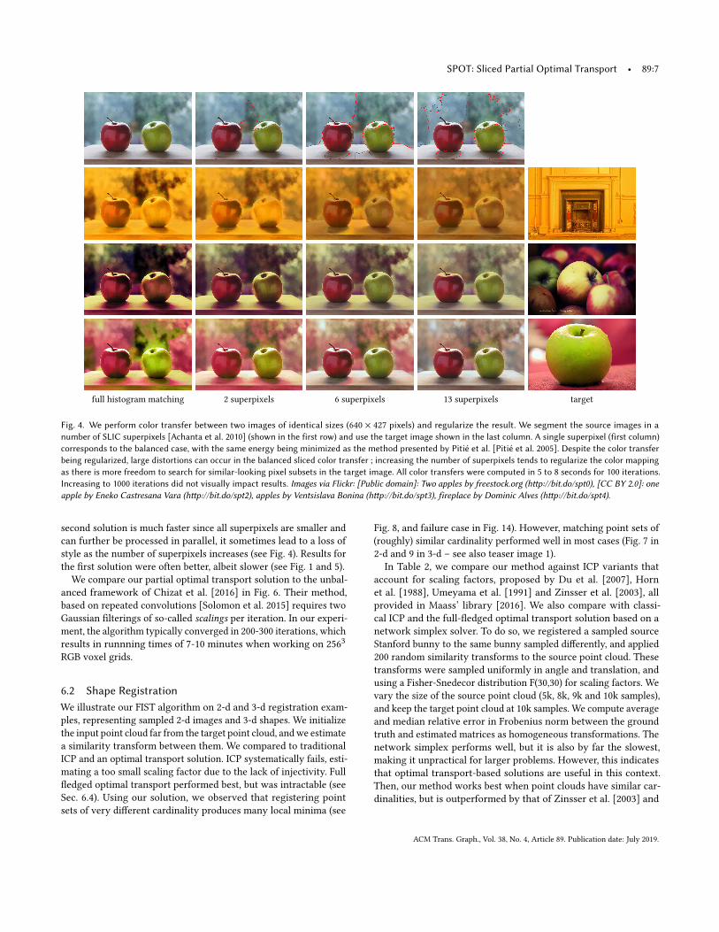
full histogram matching 2 superpixels 6 superpixels 13 superpixels target

Fig. 4. We perform color transfer between two images of identical sizes (640 × 427 pixels) and regularize the result. We segment the source images in anumber of SLIC superpixels [Achanta et al. 2010] (shown in the first row) and use the target image shown in the last column. A single superpixel (first column)corresponds to the balanced case, with the same energy being minimized as the method presented by Pitié et al. [Pitié et al. 2005]. Despite the color transferbeing regularized, large distortions can occur in the balanced sliced color transfer ; increasing the number of superpixels tends to regularize the color mappingas there is more freedom to search for similar-looking pixel subsets in the target image. All color transfers were computed in 5 to 8 seconds for 100 iterations.Increasing to 1000 iterations did not visually impact results. Images via Flickr: [Public domain]: Two apples by freestock.org (http://bit.do/spt0), [CC BY 2.0]: oneapple by Eneko Castresana Vara (http://bit.do/spt2), apples by Ventsislava Bonina (http://bit.do/spt3), fireplace by Dominic Alves (http://bit.do/spt4).

second solution is much faster since all superpixels are smaller andcan further be processed in parallel, it sometimes lead to a loss ofstyle as the number of superpixels increases (see Fig. 4). Results forthe first solution were often better, albeit slower (see Fig. 1 and 5).We compare our partial optimal transport solution to the unbal-

anced framework of Chizat et al. [2016] in Fig. 6. Their method,based on repeated convolutions [Solomon et al. 2015] requires twoGaussian filterings of so-called scalings per iteration. In our experi-ment, the algorithm typically converged in 200-300 iterations, whichresults in runnning times of 7-10 minutes when working on 2563RGB voxel grids.

6.2 Shape RegistrationWe illustrate our FIST algorithm on 2-d and 3-d registration exam-ples, representing sampled 2-d images and 3-d shapes. We initializethe input point cloud far from the target point cloud, andwe estimatea similarity transform between them. We compared to traditionalICP and an optimal transport solution. ICP systematically fails, esti-mating a too small scaling factor due to the lack of injectivity. Fullfledged optimal transport performed best, but was intractable (seeSec. 6.4). Using our solution, we observed that registering pointsets of very different cardinality produces many local minima (see

Fig. 8, and failure case in Fig. 14). However, matching point sets of(roughly) similar cardinality performed well in most cases (Fig. 7 in2-d and 9 in 3-d – see also teaser image 1).In Table 2, we compare our method against ICP variants that

account for scaling factors, proposed by Du et al. [2007], Hornet al. [1988], Umeyama et al. [1991] and Zinsser et al. [2003], allprovided in Maass’ library [2016]. We also compare with classi-cal ICP and the full-fledged optimal transport solution based on anetwork simplex solver. To do so, we registered a sampled sourceStanford bunny to the same bunny sampled differently, and applied200 random similarity transforms to the source point cloud. Thesetransforms were sampled uniformly in angle and translation, andusing a Fisher-Snedecor distribution F(30,30) for scaling factors. Wevary the size of the source point cloud (5k, 8k, 9k and 10k samples),and keep the target point cloud at 10k samples. We compute averageand median relative error in Frobenius norm between the groundtruth and estimated matrices as homogeneous transformations. Thenetwork simplex performs well, but it is also by far the slowest,making it unpractical for larger problems. However, this indicatesthat optimal transport-based solutions are useful in this context.Then, our method works best when point clouds have similar car-dinalities, but is outperformed by that of Zinsser et al. [2003] and


http://bit.do/spt0

http://bit.do/spt2

http://bit.do/spt3

http://bit.do/spt4


(a) Input (b) Target (c) Full Transfer (d) 20% Larger (e) 40% Larger[Bonneel et al. 2015] (Our method) (Our method)

Fig. 5. We transfer the colors of the target image (b) to the input (a). We either resize the images so that the problem is balanced and leads to the sameformulation as that of Pitié [Pitié et al. 2005] (c) or so that the problem becomes unbalanced using a 20% larger target image (both in width and height, columnd) or 40% (e). Images via Flickr: [CC BY 2.0]: Tree by Steve Parker (http://flic.kr/p/26TptPA), [CC BY-SA 2.0]: air balloon by Kirt Edblom (http://flic.kr/p/Ys81nY),roses by Felix Schaumburg (http://flic.kr/p/f6bkoR), clouds by Tim Wang (http://flic.kr/p/5mrPsc), White House by Diego Cambiaso (http://flic.kr/p/qbrBCJ).

(a) Full Transfer (b) Unbalanced (z = 0.99) (c) Unbalanced (z = 0.95)

[Solomon et al. 2015] [Chizat et al. 2016] [Chizat et al. 2016]

Fig. 6. For comparison, we repeat the same experiment as the first tworows of Fig. 5, but instead using the (balanced) entropy-regularized optimaltransport of Solomon et al. [2015] (a), and the unbalanced variant of Chizatet al. [2016] with two different KL constraints on marginals (using theirnotation, z1 = z2 = 0.99 (b) or 0.95 (c)). We post-processed results with thesame filtering [Rabin et al. 2010] to reduce quantization artifacts.

Umeyama et al. [Umeyama 1991] when the source point cloud onlyhas half the number of points of the target point cloud. We did notobserve significant differences between Umeyama et al. and Zinsseret al. In our experiment, classical ICP systematically resulted in

infinite average and median relative errors since in most cases, theestimated scaling factor was 0 – these values are hence not reportedin the table.Table 2. We compare our method against variants of ICP due to Du etal. [2007], Horn et al. [1988], Umeyama et al. [1991] and Zinsser at al. [2003],as well as a (slow) in-house network simplex based optimal transport so-lution [2011]. We show average (and median, in parenthesis) percentagerelative errors in Frobenius norm between ground truth and estimated trans-formations matrices. We vary the size of the source point cloud from 5k to10k samples and keep the target point cloud at 10k samples.

Method \# pts 5k 8k 9k 10kOurs 31.65 (25.53) 3.06 (1.38) 1.73 (0.15) 1.74 (0.16)

Network Simplex 26.70 (13.58) 7.85 (1.85) 3.62 (0.89) 2.14 (0.07)Du 34.04 (7.26) 33.97 (7.24) 34.02 (7.22) 34.25 (7.34)Horn 216.45 (77.53) 332.86 (82.27) INF (86.96) 168.82 (83.73)

Umeyama 21.59 (1.49) 21.58 (1.47) 21.53 (1.48) 21.69 (1.53)Zinsser 21.59 (1.49) 21.58 (1.47) 21.53 (1.48) 21.69 (1.53)

6.3 Sliced Partial BarycentersWe illustrate preliminary results on sliced partial barycenters. InFig. 10, we compute a barycenter between a cat and a dog, bothsampled with 100k points. This barycenter is a distribution of pointsin-between these two input distributions in term of optimal trans-port distances. It requires computing gradient descent steps thatmay lead to different local minimas depending on the initialization


http://flic.kr/p/26TptPA

http://flic.kr/p/Ys81nY

http://flic.kr/p/f6bkoR

http://flic.kr/p/5mrPsc

http://flic.kr/p/qbrBCJ


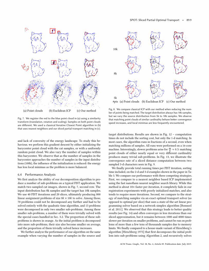
(a) Point clouds (b) Euclidean ICP (c) Our method

Fig. 7. We register the red to the blue point cloud in (a) using a similaritytransform (translation, rotation and scaling). Samples on both point cloudsare different. We used a classical Iterative Closest Point algorithm in (b)that uses nearest neighbors and our sliced partial transport matching in (c).

and lack of convexity of the energy landscape. To study this be-haviour, we perform this gradient descent by either initializing thebarycenter point cloud with the cat samples, or with a uniformlyrandom point cloud. We also vary the number of samples withinthis barycenter. We observe that as the number of samples in thebarycenter approaches the number of samples in the input distribu-tions (100k), the influence of the initialization is reduced: the energyhas less local minimas as the problem is more balanced.

6.4 Performance AnalysisWe first analyze the ability of our decomposition algorithm to pro-duce a number of sub-problems on a typical FIST application. Wematch two sampled cat images, shown in Fig. 7, second row. Theinput distribution has 8k samples and the target has 10k samples.We use 40 FIST iterations and 20 slices, ultimately producing 800linear assignment problems of size 8k × 10k to solve. Among those,70 problems could not be decomposed any further and had to besolved entirely with the quadratic time algorithm, and 13 problemswere decomposed in only two smaller sub-problems. Among thesesmaller sub-problems, a number of them were trivially solved withthe special cases handled in Sec. 3.2. The proportion of these sub-problems is shown in orange. As the initial problem is decomposedinto more sub-problems, their size also become smaller on average,and the proportion of them trivially solved hence increases.

We further analyze the performance of our algorithm on the sameexample when varying the number of samples in the source and

10k

8k

5k#pts (a) Point clouds (b) Euclidean ICP (c) Our method

Fig. 8. We compare classical ICP with our method when reducing the num-ber of points being matched. The target distribution always has 10k samples,but we vary the source distribution from 5k to 10k samples. We observethat matching point clouds of similar cardinality behave better: convergencespeed increases, and local minimas are less frequently encountered.

target distributions. Results are shown in Fig. 12 – computationtimes do not include the sorting cost, but only the 1-d matching. Inmost cases, the algorithm runs in fractions of a second, even whenmatching millions of samples. All runs were performed on a 16-coremachine. Interestingly, slower problems arise for mn ≈ 0.5: matchingpoint clouds of either nearly equal or very different cardinalityproduces many trivial sub-problems. In Fig. 13, we illustrate theconvergence rate of a sliced distance computation between twosampled 3-d characters seen in Fig. 9.

We finally provide total running times per FIST iteration, sortingtime included, on the 2-d and 3-d examples shown in the paper in Ta-ble 3. We compare our performance with three competing strategies.First, we compare to a nearest neighbor based ICP implementedusing the fast nanoflann nearest neighbor search library. While thismethod is about 10× faster per iteration, it completely fails in ourregistration experiments with poorly initialized matches, and alsotends to require more iterations. Second, we compare to the strat-egy of matching samples via an exact optimal transport solver (asopposed to optimal per slice) that uses a state-of-the-art linear pro-gramming solver based on a network simplex algorithm [Bonneelet al. 2011]. We observed that this strategy leads to better qualityresults (see Fig. 14) and often converges in less iterations than oursliced approximation, but it remains between 1000 and 4000 timesslower per iteration on smaller problems, and cannot be run on prob-lems of more than a few tens of thousands samples due to memorylimits. We finally compared to a house-made variant of Hirschberg’salgorithm [Hirschberg 1975] that first decomposes the initial prob-lem into sub-problems using Algorithm 2, and recursively solves



(a) Point clouds (b) Euclidean ICP (c) Our method

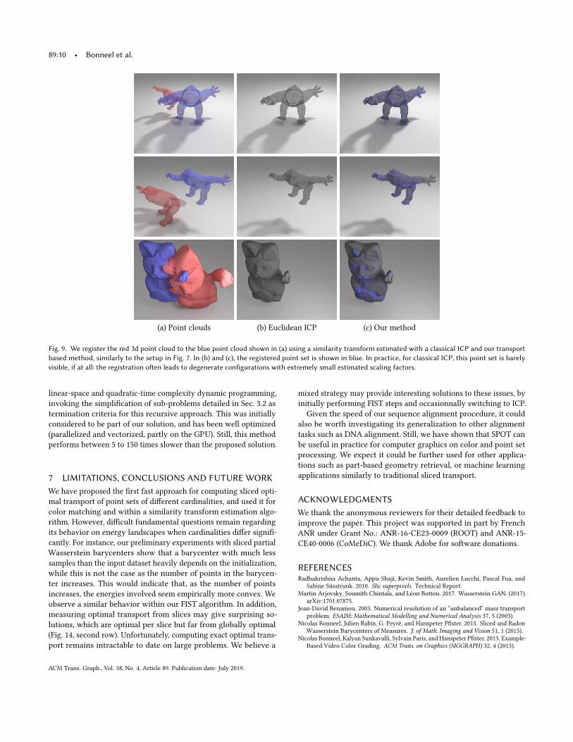
Fig. 9. We register the red 3d point cloud to the blue point cloud shown in (a) using a similarity transform estimated with a classical ICP and our transportbased method, similarly to the setup in Fig. 7. In (b) and (c), the registered point set is shown in blue. In practice, for classical ICP, this point set is barelyvisible, if at all: the registration often leads to degenerate configurations with extremely small estimated scaling factors.

linear-space and quadratic-time complexity dynamic programming,invoking the simplification of sub-problems detailed in Sec. 3.2 astermination criteria for this recursive approach. This was initiallyconsidered to be part of our solution, and has been well optimized(parallelized and vectorized, partly on the GPU). Still, this methodperforms between 5 to 150 times slower than the proposed solution.

7 LIMITATIONS, CONCLUSIONS AND FUTURE WORKWe have proposed the first fast approach for computing sliced opti-mal transport of point sets of different cardinalities, and used it forcolor matching and within a similarity transform estimation algo-rithm. However, difficult fundamental questions remain regardingits behavior on energy landscapes when cardinalities differ signifi-cantly. For instance, our preliminary experiments with sliced partialWasserstein barycenters show that a barycenter with much lesssamples than the input dataset heavily depends on the initialization,while this is not the case as the number of points in the barycen-ter increases. This would indicate that, as the number of pointsincreases, the energies involved seem empirically more convex. Weobserve a similar behavior within our FIST algorithm. In addition,measuring optimal transport from slices may give surprising so-lutions, which are optimal per slice but far from globally optimal(Fig. 14, second row). Unfortunately, computing exact optimal trans-port remains intractable to date on large problems. We believe a

mixed strategy may provide interesting solutions to these issues, byinitially performing FIST steps and occasionnally switching to ICP.Given the speed of our sequence alignment procedure, it could

also be worth investigating its generalization to other alignmenttasks such as DNA alignment. Still, we have shown that SPOT canbe useful in practice for computer graphics on color and point setprocessing. We expect it could be further used for other applica-tions such as part-based geometry retrieval, or machine learningapplications similarly to traditional sliced transport.

ACKNOWLEDGMENTSWe thank the anonymous reviewers for their detailed feedback toimprove the paper. This project was supported in part by FrenchANR under Grant No.: ANR-16-CE23-0009 (ROOT) and ANR-15-CE40-0006 (CoMeDiC). We thank Adobe for software donations.

REFERENCESRadhakrishna Achanta, Appu Shaji, Kevin Smith, Aurelien Lucchi, Pascal Fua, and

Sabine Süsstrunk. 2010. Slic superpixels. Technical Report.Martin Arjovsky, Soumith Chintala, and Léon Bottou. 2017. Wasserstein GAN. (2017).

arXiv:1701.07875.Jean-David Benamou. 2003. Numerical resolution of an “unbalanced” mass transport

problem. ESAIM: Mathematical Modelling and Numerical Analysis 37, 5 (2003).Nicolas Bonneel, Julien Rabin, G. Peyré, and Hanspeter Pfister. 2015. Sliced and Radon

Wasserstein Barycenters of Measures. J. of Math. Imaging and Vision 51, 1 (2015).Nicolas Bonneel, Kalyan Sunkavalli, Sylvain Paris, and Hanspeter Pfister. 2013. Example-

Based Video Color Grading. ACM Trans. on Graphics (SIGGRAPH) 32, 4 (2013).



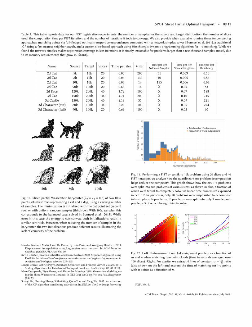
Table 3. This table reports data for our FIST registration experiments: the number of samples for the source and target distribution, the number of slicesused, the computation time per FIST iteration, and the number of iterations it took to converge. We also provide when available running times for competingapproaches: matching points via full-fledged optimal transport correspondences computed with a network simplex solver [Bonneel et al. 2011], a traditionalICP using a fast nearest neighbor search, and a custom slice-based approach using Hirschberg’s dynamic programming algorithm for 1-d matching. While wefound the network simplex makes registration converge in less iterations, it is simply intractable for problems larger than a few thousand samples, mostly dueto its memory requirements that grow in O(mn).

Name Source Target Slices Time per iter. # iter Time per iterNetwork Simplex

Time per iterNearest Neighbor

Time per iterHirschberg

2d Cat 5k 10k 20 0.03 200 31 0.003 0.152d Cat 8k 10k 20 0.04 130 40 0.005 0.562d Cat 10k 10k 20 0.04 14 155 0.006 0.042d Car 90k 100k 20 0.66 16 X 0.05 832d Face 120k 200k 40 1.72 100 X 0.07 1883d Cat 150k 200k 100 4.71 200 X 0.10 745

3d Castle 150k 200k 40 2.18 55 X 0.09 2213d Character (cut) 80k 100k 100 2.29 100 X 0.05 2743d Character (full) 90k 100k 20 0.69 100 X 0.05 40

50k 80k 100k

Fig. 10. Sliced partial Wasserstein barycenter (λ0 = λ1 = 0.5) of two 100kpoints sets (first row) representing a cat and a dog, using a varying numberof samples. The minimization is initialized with the cat point set (secondrow) or with uniform random samples (third row). With 100k samples, thiscorresponds to the balanced case, solved in Bonneel et al. [2015]. Whileeven in this case the energy is non-convex, both initializations result insimilar centroids. However, when reducing the number of samples in thebarycenter, the two initializations produce different results, illustrating thelack of convexity of the problem.

Nicolas Bonneel, Michiel Van De Panne, Sylvain Paris, and Wolfgang Heidrich. 2011.Displacement interpolation using Lagrangian mass transport. In ACM Trans. onGraphics (SIGGRAPH Asia), Vol. 30.

Kevin Charter, Jonathan Schaeffer, and Duane Szafron. 2000. Sequence alignment usingFastLSA. In International conference on mathematics and engineering techniques inmedicine and biological sciences. 239–245.

Lenaic Chizat, Gabriel Peyré, Bernhard Schmitzer, and François-Xavier Vialard. 2016.Scaling Algorithms for Unbalanced Transport Problems. Math. Comp. 87 (07 2016).

Ishan Deshpande, Ziyu Zhang, and Alexander Schwing. 2018. Generative Modeling us-ing the SlicedWasserstein Distance. In IEEE Conf. on Comp. Vis. and Patt. Recognition(CVPR).

Shaoyi Du, Nanning Zheng, Shihui Ying, Qubo You, and Yang Wu. 2007. An extensionof the ICP algorithm considering scale factor. In IEEE Int. Conf. on Image Processing

1 2 5 10 20 50 100 200Number of subproblems

0

10

20

30

40

50

60

70

Num

ber o

f occ

uren

ces

Total number of subproblemsProportion of trivial subproblems

Fig. 11. Performing a FIST on an 8k to 10k problem using 20 slices and 40FIST iterations, we analyze how the quasilinear time problem decompositionhelps reduce the compexity. This graph shows how the 800 1-d problemswere split into sub-problems of various sizes, as shown in blue, a fraction ofwhich were trivial to completely solve via linear time procedures explainedin Sec. 3.2. In particular, only 70 problems were impossible to decomposeinto simpler sub-problems, 13 problems were split into only 2 smaller sub-problems 5 of which being trivial to solve.

10k100 1k 100k 1M 5Mn

100

1k

10k

100k

1M

3M

m

1E-5

1E-4

1E-3

1E-2

1E-1

1

10

100 1k 10k 100k 1M 5Mn

10-4

10-2

100

102

time

(sec

onds

)

80%50%30%5%

Fig. 12. Left. Performance of our 1-d assignment problem as a function ofm and n when matching two point clouds (time in seconds averaged over100 slices). Right. For clarity, we extract 4 lines of constant α = m

n ratio(also shown on the left) and express the time of matching αn 1-d pointswith n points as a function of n.

(ICIP), Vol. 5.



0 50 100 150 200Number of directions

0

20

40

60

80

100

120

Rel

ativ

e pe

rcen

tage

erro

r

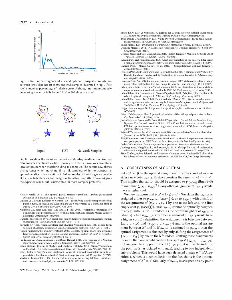
Fig. 13. Rate of convergence of a sliced optimal transport computationbetween two 3-d points set of 80k and 100k samples illustrated in Fig. 9 (firstrow) shown as percentage of relative error. Although not monotonouslydecreasing, the error falls below 1% after 200 slices are used.

Input FIST Network Simplex

Fig. 14. We show the occasional behavior of sliced optimal transport (secondcolumn) when cardinalities differ too much. In the first row, we encounter alocal optimum, when matching 5k to 10k samples. The second row showsslicing issues when matching 1k to 10k samples: while the transport isoptimal per slice, it is not optimal in 2-d as samples of the triangle are outsideof the star. In both cases, full-fledged optimal transport (third column) givesthe expected result, but is intractable for more complex problems.

Alessio Figalli. 2010. The optimal partial transport problem. Archive for rationalmechanics and analysis 195, 2 (2010), 533–560.

William A Gale and Kenneth W Church. 1991. Identifying word correspondences inparallel texts. In Speech and Natural Language: Proceedings of a Workshop Held atPacific Grove, California, February 19-22, 1991.

Xianfeng Gu, Feng Luo, Jian Sun, and S-T Yau. 2013. Variational principles forMinkowski type problems, discrete optimal transport, and discrete Monge-Ampereequations. arXiv:1302.5472 (2013).

Daniel S. Hirschberg. 1975. A linear space algorithm for computing maximal commonsubsequences. Commun. ACM 18, 6 (1975), 341–343.

Berthold KP Horn, Hugh M Hilden, and Shahriar Negahdaripour. 1988. Closed-formsolution of absolute orientation using orthonormal matrices. JOSA A 5, 7 (1988).

Hagen Kaprykowsky and Xavier Rodet. 2006. Globally optimal short-time dynamictime warping, application to score to audio alignment. In IEEE Int. Conf. on Acoustics,Speech and Signal Processing (ICASSP), Vol. 5.

Jun Kitagawa, Quentin Mérigot, and Boris Thibert. 2016. Convergence of a Newtonalgorithm for semi-discrete optimal transport. arXiv:1603.05579 (2016).

Soheil Kolouri, Charles E Martin, and Gustavo K Rohde. 2018. Sliced-WassersteinAutoencoder: An Embarrassingly Simple GenerativeModel. arXiv:1804.01947 (2018).

Soheil Kolouri, Yang Zou, and Gustavo K Rohde. 2016. Sliced wasserstein kernels forprobability distributions. In IEEE Conf. on Comp. Vis. and Patt. Recognition (CVPR).

Vladimir I Levenshtein. 1966. Binary codes capable of correcting deletions, insertions,and reversals. In Soviet physics doklady, Vol. 10. 707–710.

Bruno Lévy. 2015. A Numerical Algorithm for L2 semi-discrete optimal transport in3D. ESAIM M2AN (Mathematical Modeling and Numerical Analysis) (2015).

Tyler Lu and Craig Boutilier. 2015. Value-Directed Compression of Large-Scale Assign-ment Problems. In AAAI Conf. on Artificial Intelligence.

Edgar Maass. 2016. Point cloud alignment: ICP methods compared. Technical Report.Quentin Mérigot. 2011. A Multiscale Approach to Optimal Transport. Computer

Graphics Forum (2011).Georges Nader and Gael Guennebaud. 2018. Instant Transport Maps on 2D Grids. ACM

Trans. on Graphics (SIGGRAPH Asia) 249 (2018).Sylvain Paris and Frédo Durand. 2009. A fast approximation of the bilateral filter using

a signal processing approach. International journal of computer vision 81, 1 (2009).Gabriel Peyré, Marco Cuturi, et al. 2017. Computational optimal transport.

arXiv:1803.00567 (2017).Francois Pitié, Anil C. Kokaram, and Rozenn Dahyot. 2005. N-Dimensional Probablility

Density Function Transfer and Its Application to Colour Transfer. In IEEE Int. Conf.on Computer Vision (ICCV).

François Pitié, Anil C Kokaram, and Rozenn Dahyot. 2007. Automated colour gradingusing colour distribution transfer. Comp. Vis. and Im. Understanding 107, 1-2 (2007).

Julien Rabin, Julie Delon, and Yann Gousseau. 2010. Regularization of transportationmaps for color and contrast transfer. In IEEE Int. Conf. on Image Processing (ICIP).

Julien Rabin, Sira Ferradans, and Nicolas Papadakis. 2014. Adaptive color transfer withrelaxed optimal transport. In IEEE Int. Conf. on Image Processing (ICIP).

Julien Rabin, Gabriel Peyré, Julie Delon, and Marc Bernot. 2011. Wasserstein barycenterand its application to texture mixing. In International Conference on Scale Space andVariational Methods in Computer Vision. Springer, 435–446.

Filippo Santambrogio. 2015. Optimal transport for applied mathematicians. Birkäuser,NY (2015).

Peter H Schönemann. 1966. A generalized solution of the orthogonal procrustes problem.Psychometrika 31, 1 (1966), 1–10.

Justin Solomon, Fernando De Goes, Gabriel Peyré, Marco Cuturi, Adrian Butscher, AndyNguyen, Tao Du, and Leonidas Guibas. 2015. Convolutional wasserstein distances:Efficient optimal transportation on geometric domains. ACM Trans. on Graphics(SIGGRAPH) 34, 4 (2015).

Robert E Tarjan and Jan Van Leeuwen. 1984. Worst-case analysis of set union algorithms.Journal of the ACM (JACM) 31, 2 (1984), 245–281.

Shinji Umeyama. 1991. Least-squares estimation of transformation parameters betweentwo point patterns. IEEE Trans. on Patt. Analysis & Machine Intelligence 4 (1991).

Cédric Villani. 2003. Topics in optimal transportation. American Mathematical Soc.Jiaolong Yang, Hongdong Li, and Yunde Jia. 2013. Go-icp: Solving 3d registration

efficiently and globally optimally. In IEEE Int. Conf. on Computer Vision (ICCV).Timo Zinßer, Jochen Schmidt, and Heinrich Niemann. 2003. A refined ICP algorithm

for robust 3-D correspondence estimation. In IEEE Int. Conf. on Image Processing.

A CORRECTNESS OF ALGORITHM 1.Let a([1,m′]) be the optimal assignment of X ′ to Y and let us con-sider a new point xm′+1. First, we consider the case t(m′+1) > a(m′).This implies that xm′+1 should be assigned to yt (m′+1) (lines 4–5)to minimize

∑(xi −ya(i))

2 as any other assignment of xm′+1 wouldhave a higher cost.We now suppose that t(m′ + 1) ≤ a(m′). We claim that xm′+1 is

assigned either to ya(m′)+1 (case 2 ), or to ya(m′) with a shift ofthe assignments of {xr , . . . ,xm′} by one to the left until the firstempty spot ys (case 1 ). First, xm′+1 cannot be optimally assignedto anyyl with l > m′+1. Indeed, as the nearest neighbor of xm′+1 is(strictly) beforeya(m′)+1, any other assignment of xm′+1 would havea higher cost. By definition, the assignment a is bijective between{xr , . . . ,xm′} and {ya(r ), . . . ,xa(m′)}) and is the optimal assign-ment between X ′ and Y . If xm′+1 is assigned to ya(m′), then theoptimal assignment is obtained by only shifting the assignments of{xr , . . . ,xm′} by one to the left. Indeed, shifting those assignmentsby more than one would create a free spot yl ∈ {ya(r ), . . . ,ya(m′)}not assigned to any point in X ′ ∪ {xm′+1} (letm′′ be the index ofthe point in X ′ associated with yl−1), leading to two independentsub-problems. This would have been detected at stepm′′ of Algo-rithm 1, which is a contradiction to the fact that a is the optimalassignment of X ′ to Y . Similarly, if xm′+1 is assigned to any point



before ya(m′) the assignment would have a higher cost. Algorithm 1compares the costs of the two alternatives, 1 and 2 , to obtain theoptimal partial assignment a : {1,m′+ 1} minimizing

∑(xi −ya(i))

2.


Documents

SPOT: Sliced Partial Optimal Transport · 2019-11-08 · SPOT: Sliced Partial Optimal Transport NICOLAS BONNEEL, Univ. Lyon, CNRS DAVID COEURJOLLY, Univ. Lyon, CNRS (a) Input (b)