Embed Size (px)
Citation preview

Performance Evaluation of Arizona’s LTPP SPS-9 Project: Strategic Study of Flexible Pavement Mix Design Factors
JANUARY 2016
Arizona Department of Transportation Research Center
SPR-396-9B


Performance Evaluation of Arizona’s LTPP SPS‐9 Project: Strategic Study of Flexible Pavement Mix Design Factors
SPR‐396‐9B January 2016 Prepared by: Jason Puccinelli Nichols Consulting Engineers 1885 S. Arlington Avenue, Suite 11 Reno, NV 89505‐3370 Steven M. Karamihas The University of Michigan Transportation Research Institute 2901 Baxter Road Ann Arbor, MI 48109 Sam Shih‐Hsien Yang, Jonathan Minassian, and Kevin Senn Nichols Consulting Engineers 1885 S. Arlington Avenue, Suite 11 Reno, NV 89505‐3370 Published by Arizona Department of Transportation 206 S. 17th Avenue Phoenix, AZ 85007 In cooperation with U.S. Department of Transportation Federal Highway Administration

This report was funded in part through grants from the Federal Highway Administration, U.S.
Department of Transportation. The contents of this report reflect the views of the authors, who are
responsible for the facts and the accuracy of the data, and for the use or adaptation of previously
published material, presented herein. The contents do not necessarily reflect the official views or
policies of the Arizona Department of Transportation or the Federal Highway Administration, U.S.
Department of Transportation. This report does not constitute a standard, specification, or regulation.
Trade or manufacturers’ names that may appear herein are cited only because they are considered
essential to the objectives of the report. The U.S. government and the State of Arizona do not endorse
products or manufacturers.

Technical Report Documentation Page 1. Report No.
FHWA‐AZ‐16‐396(9B)
2. Government Accession No. 3. Recipient's Catalog No.
4. Title and Subtitle Performance Evaluation of Arizona’s LTPP SPS‐9 Project: Strategic Study of Flexible Pavement Mix Design Factors
5. Report Date
January 2016
6. Performing Organization Code
7. Author(s)
Jason Puccinelli, Steven M. Karamihas, Sam Shih‐Hsien Yang, Jonathan Minassian, and Kevin Senn
8. Performing Organization Report No.
9. Performing Organization Name and Address
Nichols Consulting Engineers 1885 South Arlington Avenue Suite 111 Reno, NV 89509‐3370 The University of Michigan Transportation Research Institute 2901 Baxter Road Ann Arbor, MI 48109
10. Work Unit No. (TRAIS)
11. Contract or Grant No.
SPR 000‐1(147) 396‐9B
12. Sponsoring Agency Name and Address
Arizona Department of Transportation 206 S. 17th Avenue Phoenix, AZ 85007
13. Type of Report and Period Covered
14. Sponsoring Agency Code
15. Supplementary Notes
Prepared in cooperation with the US Department of Transportation, Federal Highway Administration
16. Abstract As part of the Long Term Pavement Performance (LTPP) Program, the Arizona Department of Transportation (ADOT) constructed five Specific Pavement Studies 9 (SPS‐9) test sections on U.S. Route 93 near Kingman. This project, SPS‐9B, studied the effect of asphalt specifications and mix designs on flexible pavements, specifically comparing Superpave mix designs with commonly used agency designs. Opened to traffic in 1992, the project was monitored at regular intervals until the pavement was rehabilitated in 2006. Surface distress, profile, and deflection data collected throughout the life of the pavement were used to evaluate the performance of various flexible pavement design features, layer configurations, and thickness. In terms of structural cracking and smoothness, the agency standard mix design performed better than the Superpave mix designs in this study. This report documents the analyses conducted as well as practical findings and lessons learned that will be of interest to ADOT.
17. Key Words
LTPP, pavement performance, Superpave mix, profile, distress, FWD, flexible, AC, deflections, roughness, backcalculation
18. Distribution Statement
Document is available to the U.S. public through the National Technical Information Service, Springfield, VA 22161
23. Registrant's Seal
19. Security Classification
Unclassified
20. Security Classification
Unclassified
21. No. of Pages
75
22. Price

ii
SI* (MODERN METRIC) CONVERSION FACTORS APPROXIMATE CONVERSIONS TO SI UNITS
Symbol When You Know Multiply By To Find Symbol LENGTH
in inches 25.4 millimeters mm ft feet 0.305 meters m yd yards 0.914 meters m mi miles 1.61 kilometers km
AREA in2 square inches 645.2 square millimeters mm2
ft2 square feet 0.093 square meters m2
yd2 square yard 0.836 square meters m2
ac acres 0.405 hectares hami2 square miles 2.59 square kilometers km2
VOLUME fl oz fluid ounces 29.57 milliliters mL gal gallons 3.785 liters L ft3 cubic feet 0.028 cubic meters m3
yd3 cubic yards 0.765 cubic meters m3
NOTE: volumes greater than 1000 L shall be shown in m3
MASS oz ounces 28.35 grams glb pounds 0.454 kilograms kgT short tons (2000 lb) 0.907 megagrams (or "metric ton") Mg (or "t")
TEMPERATURE (exact degrees) oF Fahrenheit 5 (F-32)/9 Celsius oC
or (F-32)/1.8
ILLUMINATION fc foot-candles 10.76 lux lxfl foot-Lamberts 3.426 candela/m2 cd/m2
FORCE and PRESSURE or STRESS lbf poundforce 4.45 newtons N lbf/in2 poundforce per square inch 6.89 kilopascals kPa
APPROXIMATE CONVERSIONS FROM SI UNITS Symbol When You Know Multiply By To Find Symbol
LENGTHmm millimeters 0.039 inches in m meters 3.28 feet ft m meters 1.09 yards yd km kilometers 0.621 miles mi
AREA mm2 square millimeters 0.0016 square inches in2
m2 square meters 10.764 square feet ft2
m2 square meters 1.195 square yards yd2
ha hectares 2.47 acres ackm2 square kilometers 0.386 square miles mi2
VOLUME mL milliliters 0.034 fluid ounces fl oz L liters 0.264 gallons gal m3 cubic meters 35.314 cubic feet ft3
m3 cubic meters 1.307 cubic yards yd3
MASS g grams 0.035 ounces ozkg kilograms 2.202 pounds lbMg (or "t") megagrams (or "metric ton") 1.103 short tons (2000 lb) T
TEMPERATURE (exact degrees) oC Celsius 1.8C+32 Fahrenheit oF
ILLUMINATION lx lux 0.0929 foot-candles fc cd/m2 candela/m2 0.2919 foot-Lamberts fl
FORCE and PRESSURE or STRESS N newtons 0.225 poundforce lbf kPa kilopascals 0.145 poundforce per square inch lbf/in2
*SI is the symbol for th International System of Units. Appropriate rounding should be made to comply with Section 4 of ASTM E380. e(Revised March 2003)

iii
Contents
EXECUTIVE SUMMARY ......................................................................................................................... 1
CHAPTER 1. INTRODUCTION ................................................................................................................ 3
CHAPTER 2. SPS‐9B DEFLECTION ANALYSIS......................................................................................... 15
Analysis of Deflection Data ..................................................................................................................... 15
Maximum Deflection, Minimum Deflection, and AREA Value ............................................................... 15
Backcalculation Using the AASHTO Design Guide Procedure ................................................................ 19
Backcalculation Using Evercalc Software ............................................................................................... 22
CHAPTER 3. SPS‐9B DISTRESS ANALYSIS ............................................................................................. 27
AC Distress Types .................................................................................................................................... 27
Research Approach ................................................................................................................................. 28
Overall Performance Trend Observations .............................................................................................. 30
Key Findings from the SPS‐9B Distress Analysis ..................................................................................... 37
CHAPTER 4. SPS‐9B ROUGHNESS ANALYSIS ........................................................................................ 39
Profile Data Synchronization .................................................................................................................. 39
Data Extraction ....................................................................................................................................... 39
Cross Correlation .................................................................................................................................... 40
Synchronization ...................................................................................................................................... 41
Data Quality Screening ........................................................................................................................... 41
Summary Roughness Values ................................................................................................................... 44
Profile Analysis Tools .............................................................................................................................. 47
Detailed Observations ............................................................................................................................ 50
Summary ................................................................................................................................................. 60
CHAPTER 5. CONCLUSIONS AND RECOMMENDATIONS ...................................................................... 63
REFERENCES ....................................................................................................................................... 65
APPENDIX: ROUGHNESS VALUES ........................................................................................................ 67

iv
LIST OF FIGURES
Figure 1. Structural Layers of SPS‐9B (040900 and 04A900) ........................................................................ 3
Figure 2. Location of SPS‐9B Test Sections 040900 and 04A900 .................................................................. 5
Figure 3. SPS‐9B Test Section Layout ............................................................................................................ 6
Figure 4. SPS‐9B Test Section Layout and Details ......................................................................................... 7
Figure 5. Average Normalized Dmax by Test Section .................................................................................... 16
Figure 6. Average Normalized Dmin by Test Section .................................................................................... 17
Figure 7. AREA Values by Test Section ........................................................................................................ 18
Figure 8. Backcalculated AC Modulus by Test Section (Evercalc Method) ................................................. 24
Figure 9. Backcalculated Subgrade Resilient Modulus by Test Section (Evercalc Method) ....................... 24
Figure 10. Structural Damage Trends for SPS‐9B Test Sections .................................................................. 31
Figure 11. Environmental Damage Trends for SPS‐9B Test Sections .......................................................... 33
Figure 12. Structural Damage Index Summary ........................................................................................... 34
Figure 13. Environmental Damage Index Summary ................................................................................... 35
Figure 14. Rutting Index Summary .............................................................................................................. 36
Figure 15. IRI Progression, Section 04A901 ................................................................................................ 45
Figure 16. IRI Progression, Section 040902 ................................................................................................. 45
Figure 17. IRI Progression, Section 04A902 ................................................................................................ 46
Figure 18. IRI Progression, Section 040903 ................................................................................................. 46
Figure 19. IRI Progression, Section 04A903 ................................................................................................ 47
Figure 20. Periodic Chatter in Elevation Profiles from Section 04A901, Left Side ...................................... 51
Figure 21. Pavement Scuff in the Left Wheelpath, Section 04A901 ........................................................... 52
Figure 22. Narrow Downward Spikes in Elevation Profile, Section 040903, Visit 13 .................................. 57
Figure 23. Summary of IRI Ranges .............................................................................................................. 61
Figure 24. Comparison of HRI to MRI ......................................................................................................... 68

v
LIST OF TABLES
Table 1. Test Section Layer Thickness ........................................................................................................... 4
Table 2. Inputs for LTPP Bind v. 3.1 .............................................................................................................. 8
Table 3. SPS‐9B Mix Design Properties ......................................................................................................... 9
Table 4. Aggregate Properties for Agency Standard Marshall Mix (04A901) ............................................. 10
Table 5. SPS‐9B Mix and Binder Properties (As Constructed) ..................................................................... 11
Table 6. Climatic Information for SPS‐9B .................................................................................................... 12
Table 7. Dynamic Modulus (E*) .................................................................................................................. 13
Table 8. SPS‐9B Traffic‐Loading Summary .................................................................................................. 14
Table 9. General Trends in D0 and AREA Values (Mahoney 1995) .............................................................. 18
Table 10. Structural Parameter Statistics for SPS‐9B .................................................................................. 21
Table 11. Backcalculation Seed Value and Modulus Range ........................................................................ 22
Table 12. Backcalculation Moduli Statistics for SPS‐9B Test Sections ........................................................ 23
Table 13. Flexible Pavement Distress Types and Failure Mechanisms ....................................................... 28
Table 14. Profile Measurement Visits to the SPS‐9B Site ........................................................................... 39
Table 15. Selected Repeats, Section 04A901 .............................................................................................. 42
Table 16. Selected Repeats, Section 040902 .............................................................................................. 42
Table 17. Selected Repeats, Section 04A902 .............................................................................................. 43
Table 18. Selected Repeats, Section 040903 .............................................................................................. 43
Table 19. Selected Repeats, Section 04A903 .............................................................................................. 43
Table 20. Roughness Values ........................................................................................................................ 68

vi
List of Acronyms and Abbreviations
AASHTO American Association of State Highway and Transportation Officials
AB aggregate base
AC asphalt concrete
ADOT Arizona Department of Transportation
COV coefficient of variation
Dmax maximum deflection
Dmin minimum deflection
E* dynamic modulus
EP effective pavement modulus
ESAL equivalent single axle load
FWD falling weight deflectometer
HRI Half‐car Roughness Index
IRI International Roughness Index
ksi kips per square inch
lbf pound force
LTPP Long Term Pavement Performance
MR resilient modulus
MP milepost
MRI Mean Roughness Index
PG performance grade
PSD power spectral density
psi pounds per square inch
RN Ride Number
SHRP Strategic Highway Research Program
SN structural number
SNeff effective structural number
SPS Specific Pavement Studies

1
EXECUTIVE SUMMARY
As part of the Long Term Pavement Performance (LTPP) Program, the Arizona Department of
Transportation (ADOT) constructed five Specific Pavement Studies 9 (SPS‐9) test sections on U.S. Route
93 near Kingman. This project, SPS‐9B, studied the effect of asphalt specifications and mix designs on
flexible pavements, specifically comparing Superpave mix designs with commonly used agency designs.
The SPS‐9B test sections (040900 and 04A900) consisted of three pavement mixes with two replicate
sections. Sections 04A902 and 04A903 were both Level 1 Superpave mix designs with 25‐mm (1‐inch)
aggregate. Sections 040902 and 040903 were also Level 1 Superpave mix designs but were composed of
19‐mm (3/4‐inch) aggregate. Both Superpave mixes were performance grade (PG) 64‐16. Test section
04A901 was an agency standard mix using the Marshall mix design and containing 19‐mm aggregate.
Construction of all five sections occurred between November 1992 and August 1993, and all five
sections were placed out of study in June 2006.
This report provides general information about the project location, including climate, traffic, and
subgrade conditions, as well as details about the mix designs of each test section. The five SPS‐9B test
sections were constructed consecutively and exposed to the same traffic loading, climate, and subgrade
conditions, which allowed for direct comparisons between layer configurations and design features
without the confounding effects introduced by different in situ conditions.
Two of the sections received a slurry seal coat in 2002, which altered the profile features significantly.
The seal coat temporarily smoothed surface deterioration but did not otherwise significantly improve
environmental cracking. The sections not receiving the slurry seal had a very poor surface condition at
the end of their service lives. Most sections had a clear increase in the magnitude of environmental
distress approximately 10 years after construction. The slurry seal was applied after considerable
cracking was present. It would likely have been more effective at slowing deterioration if it had been
placed a few years earlier, prior to the development of cracking (possibly at the first sign of raveling).
The vast majority of sections showed significant growth in longitudinal cracking, and consequently
fatigue cracking. This occurred nine to 10 years after construction, with the rate of crack growth then
slowing until the sections were placed out of study. After 11 years, there was no significant difference in
structural cracking between the 19‐mm and 25‐mm mixes. All sections performed well with regard to
rut resistance. Rutting would not have triggered a rehabilitation event for any section.
The study compared the performance of the Superpave mix designs for asphalt pavements to the
agency standard mix design and found that the agency standard mix design had better performance in
terms of both structural cracking and smoothness. These findings can provide a foundation for future
design decisions, but it should be recognized that Superpave mix designs and construction practices
have evolved over the past two decades. In addition, site‐specific conditions and construction issues
may have negatively affected the performance of the Superpave mixes in this study.

2

3
CHAPTER 1. INTRODUCTION
Understanding how design features contribute to long‐term pavement performance can be extremely
valuable to pavement designers looking to optimize resources and improve overall performance. This
study’s objectives were to document the overall performance trends of the Specific Pavement Studies 9
(SPS‐9) project, identify key differences in performance between the various asphalt specifications and
mix designs, and document key findings that would be useful to the Arizona Department of
Transportation (ADOT).
This report provides the results of surface distress, deflection, and profile analyses for the Long Term
Pavement Performance (LTPP) SPS‐9 site near Kingman (the SPS‐9B project). The SPS‐9B sites were
designed to study the effect of asphalt specifications and mix designs on flexible pavements, specifically
comparing Superpave mix designs with commonly used agency designs. The two SPS‐9B projects
discussed in this report (040900 and 04A900) consist of five newly constructed sections. These sections
were constructed in conjunction with the SPS‐1 project at the same location. The five SPS‐9B test
sections consisted of three pavement mixes with two replicate sections. Sections 04A902 and 04A903
were both Level 1 Superpave mix designs with 25‐mm (1‐inch) aggregate. Sections 040902 and 040903
were also Level 1 Superpave mix designs but were composed of 19‐mm (3/4‐inch) aggregate. Both
Superpave mixes were performance grade (PG) 64‐16. Test section 04A901 was an agency standard mix
using the Marshall mix design and containing 19‐mm aggregate.
All five SPS‐9B test sections had the same thickness design; each consisted of approximately 7 inches of
asphalt concrete laid over 4 inches of granular base placed on top of subgrade. Figure 1 depicts a
structural cross section of the sites as originally constructed.
Note: Layer thicknesses are approximate. Sites 040902 and 04A902 received a 0.5‐inch slurry seal in 2002 (not shown).
Figure 1. Structural Layers of SPS‐9B (040900 and 04A900)
7” Asphalt Concrete
4” Granular Base
Subgrade

4
After original construction in 1992 to 1993, the following maintenance activities were performed:
040902 (Superpave mix, Level 1, PG 64‐16, 19 mm): Slurry seal in 2002.
040903 (Superpave mix, Level 1, PG 64‐16, 19 mm): No rehabilitation or maintenance
conducted.
04A901 (agency standard mix, 19 mm): No rehabilitation or maintenance conducted.
04A902 (Superpave mix, Level 1, PG 64‐16, 25 mm): Crack seal in 2001; slurry seal in 2002.
04A903 (Superpave mix, Level 1, PG 64‐16, 25 mm): No rehabilitation or maintenance
conducted.
All test sections were placed out of study due to reconstruction in the summer of 2006.
Table 1 lists the test section structural properties in further detail. As previously mentioned, Sections
040902 and 04A902 received a 0.5‐inch slurry seal in 2002. The LTPP construction report (Nichols
Consulting Engineers 1997) provides more detail on the layout and structural properties of the site.
Table 1. Test Section Layer Thickness
Section Granular Base Thickness
(inches) Asphalt Concrete Thickness
(inches)
040902 4 7*
040903 4 6.6
04A901 4 6.9
04A902 4 6.5*
04A903 4 6.7
*0.5‐inch slurry seal applied in 2002.
The test pavements were constructed on northbound U.S. Route 93 in Mohave County, Arizona, from
November 1992 to August 1993. The site extends from milepost 53.23 to milepost 46.43, which is north
of Kingman and south of the Nevada/Arizona border. The terrain surrounding the test section is slightly
rolling, and the roadway is straight with grades reaching 3 percent in some areas. The soil is covered
with various desert‐type brush and small trees. Low foothills surround the test section in the distance.
The approximate elevation of the test section is 3523 ft, with a latitude of 35° 23’ and longitude
of ‐114° 15’. The location and layout of the SPS‐9B project are shown in Figures 2 through 4. The five
SPS‐9B test sections were constructed concurrently with the SPS‐1 project. The performance of the
SPS‐1 project is discussed in a separate report (Puccinelli et al. 2012).
5
The test sections are located entirely on a shallow fill of native material. The subgrade and embankment
material are a coarse‐grained silty sand with gravel and cobbles.
During paving, both Superpave mixtures were susceptible to segregation. This segregation was
attributed to the coarseness of the mixes and to worn kickback paddles on the paver. This caused areas
with significant surface voids. However, ADOT reported that after three months of traffic, the surfaces
of the Superpave mixtures appeared less bony and were no longer rich‐looking. At this point,
segregation did not seem to be a problem.
Figure 2. Location of SPS‐9B Test Sections 040900 and 04A900
(Courtesy of Google Maps)

6
Figure 3. SPS‐9 Test Section Layout
7
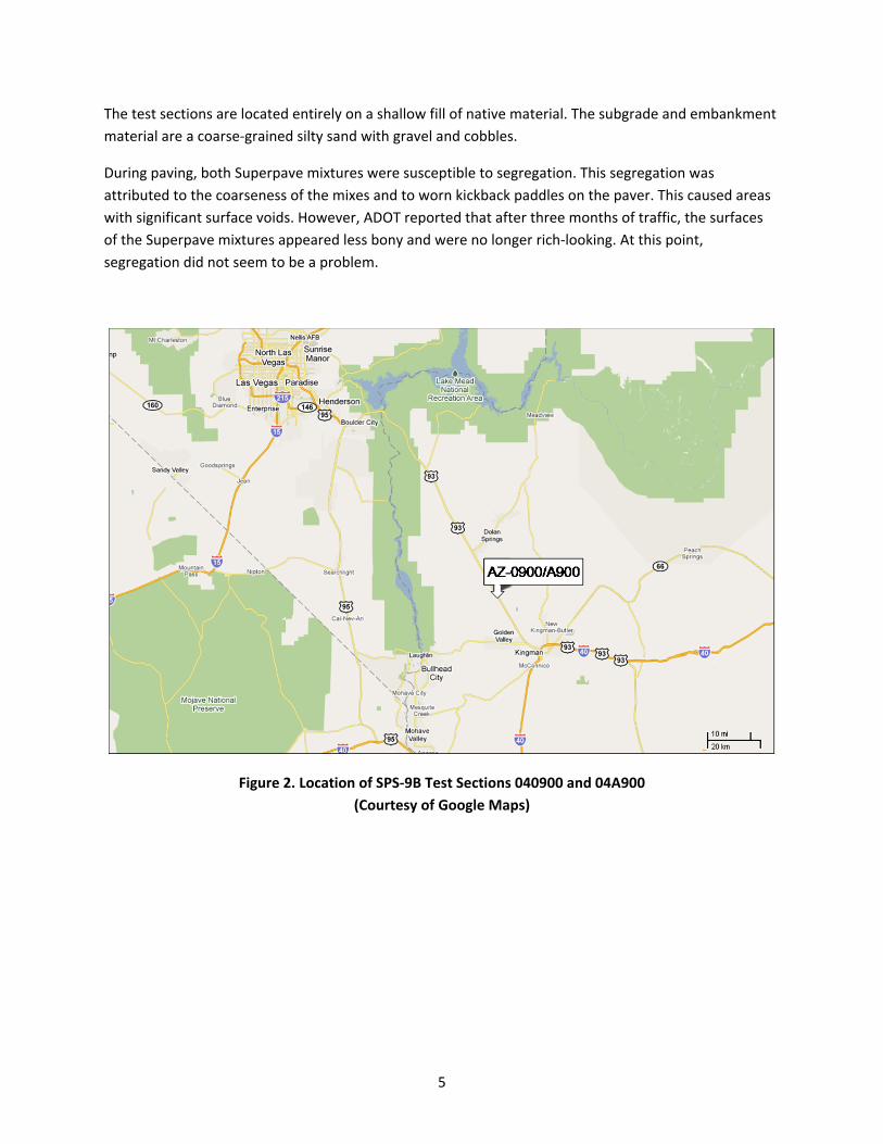
Within the SPS‐9 experiment, early projects such as 040900 and 04A900 were designated SPS‐9P, with the “P” standing for pilot. The test
sections were designed and constructed according to interim Superpave specifications then available, some of which were revised following
construction of the SPS‐9P projects. Additional changes internal to the LTPP program regarding materials sampling and testing requirements for
SPS‐9 applied to projects constructed later and not to the SPS‐9P projects. These changes were not unexpected, and the SPS‐9P sections were
nominated and selected with the understanding that Superpave modifications would occur. It was determined by the Strategic Highway
Research Program (SHRP) and by the participating state and provincial highway agencies that it was more important to develop experience
implementing Superpave specifications than to wait until everything had been finalized.
Figure 4. SPS‐9P Test Section Layout and Details
Station
(ft)
SHRP ID
Original Pavement Configuration
AC Base and Subbase
Thick(in) Type
Thick(in) Type
Base and Subbase
Type
040902
04A902
972+00
977+00985+00
990+00
Distance
(m)
152.4
152.4
04A901
1162+75
1167+75
152.4
04A903
1309+42
1314+42
152.4
040903
1320+42
1325+42
152.4
4.07.0
6.5
6.9
6.7
7.0
4.0
4.0
4.0
4.0
Dense Grade AC
Mix Design Binder Grade
Dense Grade AC
Crush Stone, Gravel/ Slag
Crush Stone, Gravel/ Slag
Silty Sand
Silty Sand
Dense Grade AC
Dense Grade AC
Dense Grade AC
Coarse Grained Soil : Silty Sand with Grav el
Coarse Grained Soil : Well Graded Grav el with Silt and Sand
Coarse Grained Soil : Silty Sand with Grav el
Crushed Gravel
Crushed Gravel
Crushed Gravel
Superpave Level I: ¾ in (19mm)
Superpave Level I: ¾ in (19mm)
ADOT Standard (Marshall Design): ¾ in
(19mm)
Superpave Level I: 1 in (25mm)
Superpave Level I: 1 in (25mm)
AC-30(=PG 64-16)
AC-30(=PG 64-16)
AC-30(=PG 64-16)
AC-30(=PG 64-16)
AC-30(=PG 64-16)

8
As mentioned previously, the five test sections were used to compare three different scenarios, with
two replicate tests. The test sections were constructed using different asphalt specifications and mix
designs. Sections 040902 and 040903 were Superpave Level 1 mixes with 19‐mm gradations, Sections
04A902 and 04A903 were Superpave Level 1 mixes with 25‐mm gradations, and Section 04A901 was a
standard agency mix using a 75‐blow Marshall mix design with a 19‐mm gradation. However, because
the asphalt binder, AC‐30, met both the agency standard and the Superpave design specification, it was
used for all five test sections. Using the LTPP Bind 3.1 software, the recommended binder for this project
site was PG 76‐10. The inputs used in the program are shown in Table 2.
Table 2. Inputs for LTPP Bind v. 3.1
Latitude 35.2°
Lowest yearly air temperature ‐8.8° C
Yearly degree‐days greater than 10° C 3884
Low air temperature standard deviation 3.1° C
Desired reliability 98%
Depth of layer 0 mm
Traffic speed Fast
Traffic loading Up to 3 million ESALs
Table 3 shows the mix design properties of each test section, Table 4 shows the mix property test
results, and Table 5 shows the mix and binder properties as constructed. The Superpave mix design
required an AC content of approximately 5 percent to achieve 4.0 percent air voids. This was noticeably
more binder than the agency mix design required to achieve the same amount of air voids. In fact, the
agency mix with a 5 percent AC content would have yielded only 2 to 3 percent air voids (Sebaaly et al.
2001).

9
Table 3. SPS‐9B Mix Design Properties
Property 040902 040903 04A901 04A902 04A903
Mix type Superpave Superpave Marshall Specification Superpave Superpave
Asphalt binder AC‐30
PG 64‐16 AC‐30
PG 64‐16 AC‐30 N/A
AC‐30 PG 64‐16
AC‐30 PG 64‐16
Maximum specific gravity
2.509 2.509 N/A N/A 2.523 2.523
Bulk specific gravity 2.406 2.406 N/A N/A 2.422 2.422
Specific gravity of aggregate blend
2.670 2.670 N/A N/A 2.683 2.683
Aggregate effective specific gravity
2.724 2.724 N/A N/A 2.727 2.727
Specific gravity of binder (Gb)
1.03 1.03 N/A N/A 1.03 1.03
Asphalt content (%) 5.2 5.2 4.1 N/A 4.9 4.9
Air voids (%) 4.1 4.1 5.6 5.3–5.7 4.0 4.0
Mineral aggregate air voids (%)
14.6 14.6 14.5 14.5–17.0 14.2 14.2
Voids filled with asphalt (%)
73.0 73.0 61.4 N/A 72.0 72.0
Asphalt absorption (%) 0.8 0.8 N/A N/A 0.6 0.6
Effective asphalt content (%)
4.4 4.4 3.9 N/A 4.3 4.3
Marshall stability (lb) 3500 3500 5013 2990 min. 3800 3800
Immersion compression retention
N/A N/A 83.9 50 min. N/A N/A
Number of blows 75 75 75 N/A 75 75
Marshall flow value (1 x 10‐2 inches)
15 15 10 N/A 17 17
Number of gyrations in Superpave Gyratory Compactor
113 113 113 N/A 113 113
Density (kg/m3) 2406 2406 2385 N/A 2423 2423
Percentage of maximum specific gravity at initial number of gyrations (% Gmm @ Nini)
86.7 86.7 N/A N/A 86.0 86.0
Percentage of maximum specific gravity at maximum number of gyrations (% Gmm @ Nmax)
98.3 98.3 N/A N/A 98.2 98.2
Tensile strength ratio (%) N/A N/A N/A N/A 82.6 82.6
N/A: Not available.

10
Table 4. Aggregate Properties for Agency Standard Marshall Mix (04A901)
Property Test Result Specification
Bulk oven‐dried specific gravity (combined)
2.673 2.35–2.85
Saturated surface‐dry specific gravity (combined)
2.693 N/A
Apparent specific gravity (combined)
2.72 N/A
Asphalt absorption (combined) (%) 0.756 0–2.50
Sand equivalent 64 45 min.
Plasticity index Nonplastic N/A
Crushed faces 98 70 min.
LA abrasion test, 100 revolutions (% loss)
6 9 max.
LA abrasion test, 500 revolutions (% loss)
25 40 max.
N/A: Not available.

11
Table 5. SPS‐9B Mix and Binder Properties (As Constructed)
040902 040903 04A901 04A902 04A903
Mix type Superpave Superpave Marshall Superpave Superpave
In situ density (kg/m3) 2335 2345 2191 2302 2311
Average core thickness (inches) 7.10 6.64 6.87 6.51 6.73
Maximum specific gravity 2.555 2.507 N/A 2.520 2.524
Average bulk specific gravity of cores
2.355 2.324 2.328 2.369 2.365
AASHTO T‐283 tensile strength ratio
0.616 0.750 N/A 0.611 0.670
Asphalt content (%) 4.3 4.2 N/A 4.7 4.9
Abson ash content (%) 0.4 0.2 N/A 0.3 0.2
Air voids (%) 7.8 7.3 N/A 6.0 6.3
Coarse aggregate Bulk specific gravity Asphalt absorption (%)
2.66 0.7
2.67 0.9
N/A
2.73 0.6
2.69 0.7
Fine aggregate Bulk specific gravity Asphalt absorption (%)
2.64 1.0
2.62 1.1
N/A
2.62 1.3
2.63 1.3
Recovered asphalt cement Penetration at 25° C (mm) Penetration at 46° C (mm) Penetration index Kinematic viscosity at 135° C (centistokes) Absolute viscosity at 60° C (poise)
31 144 1.6 686
10,824
33 161 1.4 N/A
N/A
N/A
54 258 1.5 482
4144
35 150 2.0 668
8947
Specific gravity of AC 1.040 1.042 N/A 1.043 1.039
Gradation (percentage of aggregate passing metric sieves) 37.5 mm 25.0 mm 19.0 mm 12.5 mm 9.5 mm 4.75 mm 2.00 mm 0.425 mm 0.180 mm 0.075 mm
100 100 97 67 51 33 17 8 5 2.6
100 100 96 69 54 35 19 10 6 3.6
N/A
100 96 84 70 62 43 24 12 7 4.0
100 95 88 74 65 46 24 11 6 4.0
Average MR value at 5° C at 25° C at 40° C
9.827 3.18 0.94
11.5 3.125 0.955
11.99 4.2 1.55
9.175 2.91 0.935
10.655 3.425 1.165
N/A: Not available.
12
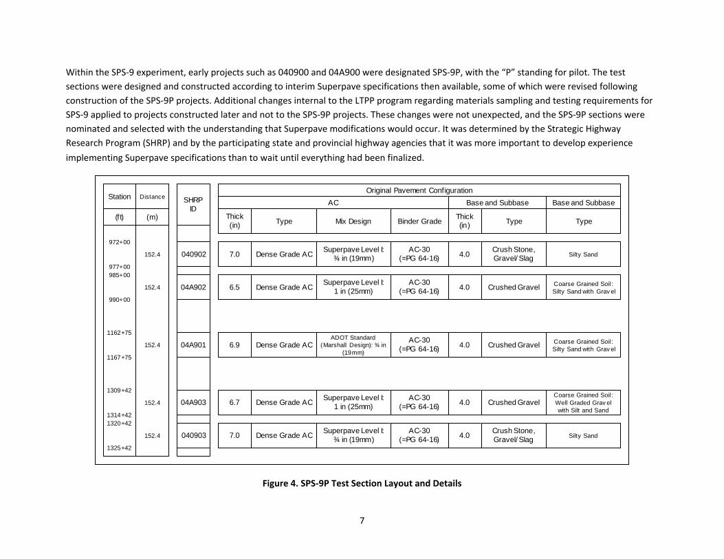
By LTPP definitions, the SPS‐9 project site is a dry, no‐freeze environment (Table 6). The temperature
and precipitation information in Table 6 represents 40 years of recorded data collected at nearby
weather stations. The solar radiation and humidity data were summarized from 14 years of on‐site
weather station data.
Table 6. Climatic Information for SPS‐9B
40‐Year Average
40‐Year Maximum
40‐Year Minimum
Annual average daily mean temperature (°F) 67 71 62
Annual average daily maximum temperature (°F) 80 85 75
Annual average daily minimum temperature (°F) 53 58 49
Absolute maximum annual temperature (°F) 111 118 103
Absolute minimum annual temperature (°F) 22 30 8
Number of days per year above 32° F 130 168 89
Number of days per year below 32° F 22 53 4
Annual average freezing index (°F‐days) 3 27 0
Annual average precipitation (inches) 8.1 17.5 3.1
Annual average daily mean solar radiation (W/ft2) 21.3 39.8 1.1
Annual average daily maximum relative humidity (%) 54 66 45
Annual average daily minimum relative humidity (%) 18 23 14
13
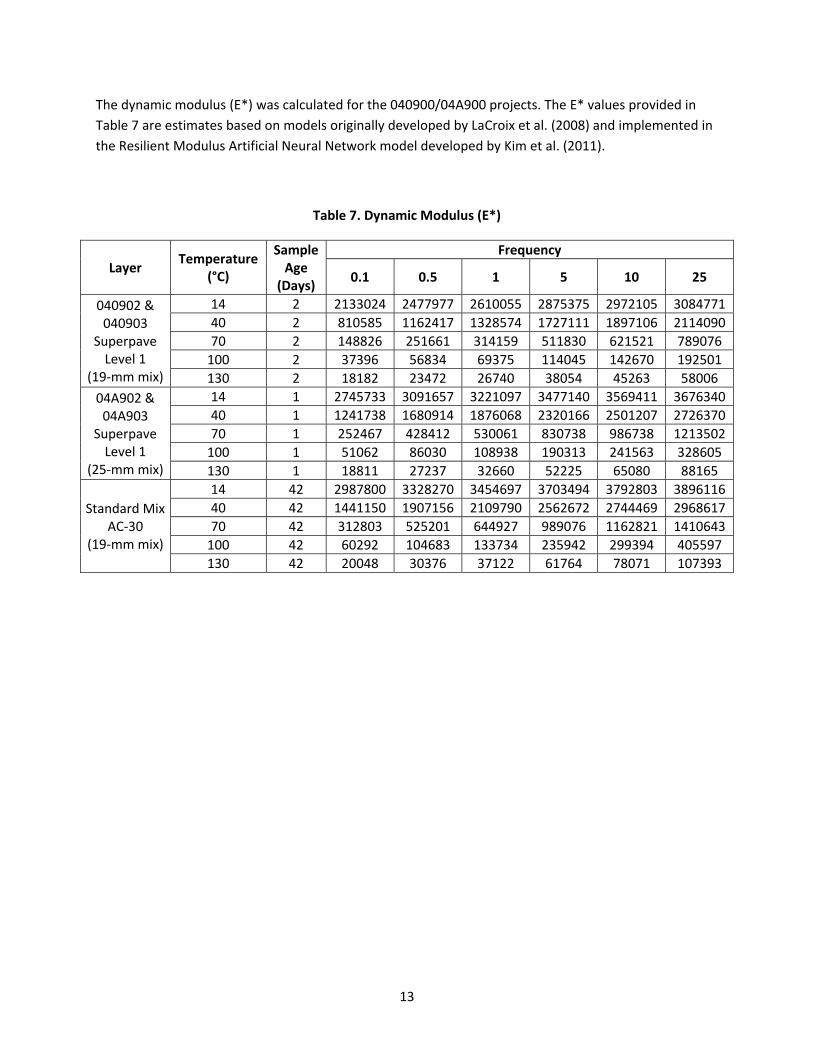
The dynamic modulus (E*) was calculated for the 040900/04A900 projects. The E* values provided in
Table 7 are estimates based on models originally developed by LaCroix et al. (2008) and implemented in
the Resilient Modulus Artificial Neural Network model developed by Kim et al. (2011).
Table 7. Dynamic Modulus (E*)
Layer Temperature
(°C)
Sample Age
(Days)
Frequency
0.1 0.5 1 5 10 25
040902 & 040903
Superpave Level 1
(19‐mm mix)
14 2 2133024 2477977 2610055 2875375 2972105 3084771
40 2 810585 1162417 1328574 1727111 1897106 2114090
70 2 148826 251661 314159 511830 621521 789076
100 2 37396 56834 69375 114045 142670 192501
130 2 18182 23472 26740 38054 45263 58006
04A902 & 04A903
Superpave Level 1
(25‐mm mix)
14 1 2745733 3091657 3221097 3477140 3569411 3676340
40 1 1241738 1680914 1876068 2320166 2501207 2726370
70 1 252467 428412 530061 830738 986738 1213502
100 1 51062 86030 108938 190313 241563 328605
130 1 18811 27237 32660 52225 65080 88165
Standard Mix AC‐30
(19‐mm mix)
14 42 2987800 3328270 3454697 3703494 3792803 3896116
40 42 1441150 1907156 2109790 2562672 2744469 2968617
70 42 312803 525201 644927 989076 1162821 1410643
100 42 60292 104683 133734 235942 299394 405597
130 42 20048 30376 37122 61764 78071 107393

14
Table 8 summarizes the total equivalent single axle loads (ESALs) computed from traffic‐loading
information collected at the SPS‐9 site. For 1993 and 2002, no monitoring traffic data were available.
The ESAL value for 1993 was derived from estimates provided by ADOT. The significant reduction in
ESALs after 2001 is due to the restriction of truck traffic on Hoover Dam implemented following
September 11.
Table 8. SPS‐9B Traffic‐Loading Summary
Year ESALs
1993 230,000*
1994 231,090
1995 252,299
1996 273,576
1997 260,773
1998 282,142
1999 299,002
2000 351,006
2001 380,213
2002 N/A
2003 52,847
2004 57,257
2005 46,917
*ADOT traffic estimate. No monitoring data available. N/A: Not available.
Three analyses were conducted on the SPS‐9B project to evaluate pavement performance: deflection,
distress, and profile. The remaining chapters of this report address each analysis, including a description
of the research approach along with performance comparisons between test sections, overall trends, a
summary of the results, and key findings.

15
CHAPTER 2. SPS‐9B DEFLECTION ANALYSIS
Falling weight deflectometer (FWD) data provide information about the overall strength (i.e., stiffness)
of the pavement structure and individual layers. At the SPS‐9B site, researchers used this information to
evaluate changes with time or, as in the case of the asphalt‐bound layers, temperature. The researchers
conducted additional analyses to gain insight on how various design features affect structural
performance.
ANALYSIS OF DEFLECTION DATA
Using the nondestructive FWD deflection testing data, researchers can identify the structural condition
of the sections over their service life. In this chapter, three levels of analysis are presented. First,
researchers produced the deflection profile plots of maximum deflection (D0), minimum deflection
(D7/ D8), and AREA value for all sections as a preliminary analysis to identify changes in the pavement
and subgrade over time. Next, they backcalculated the subgrade resilient modulus (MR), effective
pavement modulus (EP), and effective structural number (SNeff) as outlined in the AASHTO Guide for
Design of Pavement Structures (AASHTO 1993). Finally, they backcalculated asphalt concrete (AC)
modulus and MR using industry standard software.
MAXIMUM DEFLECTION, MINIMUM DEFLECTION, AND AREA VALUE
Maximum Deflections
The normalized average maximum deflection (D0, measured at the center of the FWD load plate,
normalized to a load level of 9000 pounds and an AC mix temperature of 68° F) typically indicates the
total stiffness of the pavement structure (surface and base) and the underlying subgrade. Increases in
the normalized average maximum deflection (or Dmax) observed over time may be due to weakening of
the pavement structure, weakening of the subgrade, or both.
Figure 5 shows Dmax results for each test section from the first round of testing to the last. Except for
Section 04A901, the first round of testing for all sections was performed in February 1994. The first
round of tests for section 04A901 was performed in January 1998. The last round of testing for all
sections was performed in April 2005.

16
Figure 5. Average Normalized Dmax by Test Section
Minimum Deflections
The minimum deflection (Dmin) is observed in the sensor farthest from the loading plate, which for LTPP
can be either sensor No. 7 or sensor No. 8, depending on the configuration used. Dmin readings are also
normalized to a standard 9000 pounds, but no temperature correction factor is applied. Dmin readings
are indicative of the subgrade characteristics. Figure 6 shows the Dmin measurement from the first round
of testing to the last. Four rounds of testing were conducted on Section 04A901, and six rounds of
testing were conducted on the remaining sections. Similar deflection responses were observed in
Sections 04A901, 04A903, and 040903, where the deflection value was higher than that measured in
Sections 04A902 and 040902. The average Dmin in Sections 04A901, 04A903, and 040903 was about
0.9 mils, and the average Dmin in Sections 04A902 and 040902 was about 0.6 mils.
0
5
10
15
20
A901 A902 0902 A903 0903Dm
axN
orm
aliz
ed t
o 9
000
lbs,
68°
F (
mils
)
AZ SPS-9B Test Section
1994 1995 1998 1999 2002 2005
04A901 04A902 040902 04A903 040903

17
Figure 6. Average Normalized Dmin by Test Section
AREA Value
The AREA parameter is commonly used as a means of quantifying the relative stiffness of a pavement
section. The equation for the AREA value is (AASHTO 1993):
A = 6(D0 + 2D1 + 2D2 + D3)/D0 (Eq. 1)
Where A = area value
D0 = surface deflection at the center of the test load
D1 = surface deflection at 12 inches
D2 = surface deflection at 24 inches
D3 = surface deflection at 36 inches
The AREA value is the normalized area of a slice taken through any deflection basin between the center
of the loaded area and 36 inches. This area is said to be normalized because it is divided by the
0
0.5
1
1.5
2
A901 A902 0902 A903 0903
Dm
inN
orm
aliz
ed t
o 9
000
lbs
(mils
)
AZ SPS-9B Test Section
1994 1995 1998 1999 2002 2005
04A901 04A902 040902 04A903 040903
18
maximum deflection, D0. The maximum value of the AREA parameter is 36 inches, which occurs when all
four deflection values are equal. This would result from testing an extremely rigid section of pavement.
The minimum AREA value is 11.02 inches, which would result from deflection measurements on a one‐
layer system of homogeneous material. This would imply that the pavement structure is of the same
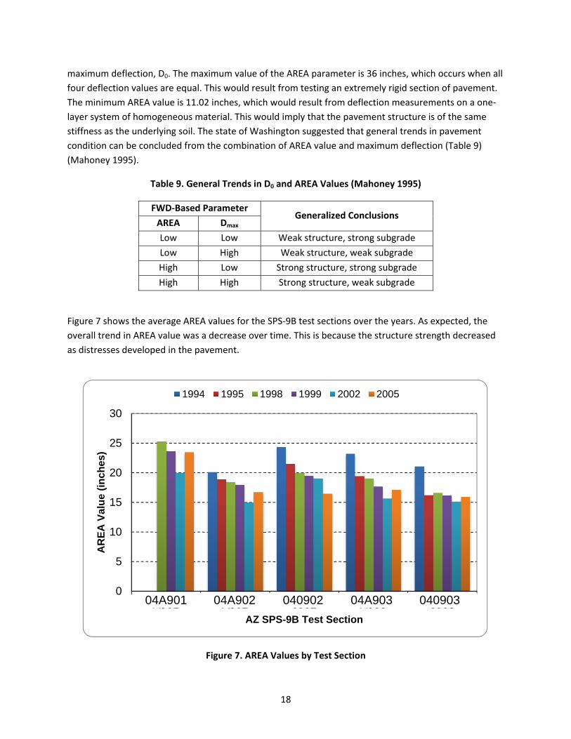
stiffness as the underlying soil. The state of Washington suggested that general trends in pavement
condition can be concluded from the combination of AREA value and maximum deflection (Table 9)
(Mahoney 1995).
Table 9. General Trends in D0 and AREA Values (Mahoney 1995)
FWD‐Based Parameter Generalized Conclusions
AREA Dmax
Low Low Weak structure, strong subgrade
Low High Weak structure, weak subgrade
High Low Strong structure, strong subgrade
High High Strong structure, weak subgrade
Figure 7 shows the average AREA values for the SPS‐9B test sections over the years. As expected, the
overall trend in AREA value was a decrease over time. This is because the structure strength decreased
as distresses developed in the pavement.
Figure 7. AREA Values by Test Section
0
5
10
15
20
25
30
A901 A902 0902 A903 0903
AR
EA
Val
ue
(in
ches
)
AZ SPS-9B Test Section
1994 1995 1998 1999 2002 2005
04A901 04A902 040902 04A903 040903

19
Sections 04A902 and 04A903 were both constructed using Superpave Level I mix with 25‐mm nominal
aggregate size, but the AREA values are larger in Section 04A903 than in Section 04A902. In addition, the
minimum deflection in 04A902 is smaller than in 04A903. This implies that the subgrade is stronger in
04A902 than in 04A903. Thus, the structure strength above the subgrade in 04A902 is much weaker
than in 04A903. By contrast, Section 040903 has generally lower AREA values than Section 040902,
indicating that 040903 is a stronger pavement overall.
BACKCALCULATION USING THE AASHTO DESIGN GUIDE PROCEDURE
The 1993 AASHTO Guide for Design of Pavement Structures (AASHTO 1993) outlines a procedure for
calculating MR, the effective modulus of all pavement layers above the subgrade, and SNeff using
measured deflection data. The deflections, which are measured at a distance of at least 0.7 times the
radius of the stress bulb at the subgrade‐pavement interface, are considered to reflect the deformation
of the subgrade layer only and hence can be used to compute MR. The backcalculated MR can be
calculated as:
R
R rD
PM
21
(Eq. 2)
Where MR = backcalculated subgrade resilient modulus
μ = Poisson’s ratio (μ = 0.5 was assumed in the analysis)
P = applied load (lbf)
r = distance from the center of the load plate to Dr (inches)
Dr = pavement surface deflection at distance r from the center of the load plate (inches)
The radius of the stress bulb can be determined from the following equation:
R
Pe M
EDaa 32
(Eq. 3)

20
Where ae = radius of the stress bulb at the subgrade‐pavement interface (inches)
a = FWD load plate radius (inches)
D = total thickness of pavement layers (inches)
EP = effective pavement modulus
MR = backcalculated subgrade resilient modulus
To obtain EP in this equation, the researchers used an equation linking the FWD deflection at the center
plate (Dmax), EP, and MR:
p
R
pR
E
a
D
M
E
a
DM
Pad
2
3
0
1
11
1
15.1 (Eq. 4)
Where d0 = deflection at the pavement surface (inches), adjusted to a standard temperature of
68° F
P = contact pressure under the loading plate (psi)
a = load plate radius (inches)
D = actual pavement structure thickness (inches)
MR = subgrade resilient modulus (psi)
EP = effective modulus of the pavement structure (psi)
Once EP was determined, SNeff could be calculated:
SNeff = (0.0045) (D) (EP)0.33 (Eq. 5)

21
Where SNeff = effective structural number
D = total thickness of the pavement structure above the subgrade (inches)
EP = effective modulus of the pavement structure above the subgrade (psi)
To accommodate the large quantity of data, the researchers developed a spreadsheet to calculate MR,
EP, and SNeff for each test section. Table 10 presents the statistics of these structural parameters.
Table 10. Structural Parameter Statistics for SPS‐9B
Section Date MR (psi) EP (psi)
SNeff Average Maximum Minimum
COV(%)
Average Maximum Minimum COV (%)
04A901
1998 35,139 55,370 24,515 29.7 498,636 614,634 452,228 8.7 3.81
1999 32,559 52,153 21,523 34.7 440,233 551,078 238,315 17.6 3.66
2002 36,825 70,533 21,267 43.3 497,738 636,591 394,578 14.3 3.68
2005 30,277 47,701 20,761 28.9 564,082 701,365 267,296 21.4 3.86
04A902
1994 40,516 59,080 30,069 20.9 257,499 330,556 130,614 26.3 2.64
1995 31,850 48,152 25,516 19.0 192,128 389,925 50,390 66.1 1.93
1998 30,504 38,197 24,257 11.8 134,876 292,195 40,179 72.1 1.67
1999 27,665 32,782 23,529 11.3 125,552 294,307 44,668 69.8 1.71
2002 32,725 43,584 25,824 14.8 125,464 222,999 89,133 36.0 2.13
2005 29,577 35,283 24,127 10.9 145,526 275,853 79,105 54.2 2.15
040902
1994 30,656 33,680 27,636 7.1 230,124 262,850 186,866 11.2 2.90
1995 28,014 30,615 26,402 4.7 104,787 168,434 68,446 30.2 2.16
1998 29,626 34,155 24,129 15.1 60,127 80,121 42,441 23.6 1.80
1999 28,619 34,478 23,468 13.2 61,886 83,857 48,393 21.5 1.83
2002 34,678 53,887 26,363 23.0 108,332 144,199 84,104 19.4 2.31
2005 29,191 33,535 25,061 9.9 112,618 193,695 66,031 38.1 2.21
04A903
1994 25,904 29,923 22,054 7.5 271,533 341,231 179,841 17.3 2.97
1995 21,064 26,043 18,395 10.5 149,606 250,362 69,093 36.7 2.22
1998 19,955 29,331 17,671 17.2 96,673 255,403 45,201 60.5 1.91
1999 23,162 25,683 19,536 8.7 77,267 225,921 44,419 67.7 1.75
2002 23,782 27,304 20,858 9.1 124,220 212,588 93,600 27.6 2.24
2005 19,865 27,846 17,357 14.4 74,964 145,494 52,234 36.4 1.83
040903
1994 22,921 24,088 20,983 3.9 169,272 239,053 110,939 27.1 2.34
1995 21,925 24,546 20,400 5.0 64,789 76,239 53,040 10.9 1.84
1998 21,482 23,119 20,157 4.7 49,969 57,621 44,267 7.9 1.71
1999 21,704 23,367 19,867 4.9 48,929 54,584 43,339 7.8 1.69
2002 23,567 25,026 22,239 4.5 98,316 114,552 86,155 8.1 2.14
2005 20,401 22,458 18,600 5.8 66,207 73,640 58,682 7.4 1.88

22
Section 04A901 had an MR of 35 ksi in 1998, but MR had decreased by 20 percent at the last round of
testing in 2005. EP increased from 498 ksi at the first round of testing in 1998 to 564 ksi in 2005. Section
04A901 showed little variation in SNeff over time. Sections 04A902 and 040902 contained 1 inch and ¾ inch
of Superpave Level I mix, respectively. In both sections, EP and SNeff showed a declining trend over time.
Similar trends can also be observed in the replicate sections of 04A903 and 040903.
BACKCALCULATION USING EVERCALC SOFTWARE
The researchers also processed the FWD data using the backcalculation software Evercalc, which was
developed by the Washington State Department of Transportation. One set of FWD data at each station
was selected for backcalculation using the representative thickness of each test section obtained from
the LTPP database to determine MR of each layer. Table 11 shows the seed value and modulus range
used for backcalculation. The pavement structure was first assumed to be a four‐layer system: asphalt
concrete, aggregate base, subgrade, and bedrock. However, after running several initial analyses,
researchers found that the base layer was not producing reasonable moduli values. Consequently,
instead of calculating each individual layer modulus, researchers combined the base layer with the
subgrade layer and repeated the backcalculation analysis. This approach produced more reasonable
moduli values.
Table 11. Backcalculation Seed Value and Modulus Range
Layer Seed Modulus
(ksi) Poisson’s Ratio
Minimum Modulus (ksi)
Maximum Modulus (ksi)
Asphalt concrete 400 0.35 100 2100
Aggregate base 25 0.3 10 150
Subgrade 15 0.4 5 50
Table 12 provides the statistics on the backcalculated moduli for the test sections. (The information in
Table 12 is also shown graphically in Figures 8 and 9.) In general, backcalculated AC modulus decreased
as pavement age increased, potentially caused by the progression of pavement distresses over time.
Except in Section 04A901, there is a significant trend in AC moduli decreasing over time. In the case of
04A902, the AC moduli decreased after the first round of testing, and the values bounced back at the
last round of testing. The values also bounced back in Section 040902, but in the second to last round of
testing. The resulting trend coincides with other parameters discussed in the previous section. A similar
decreasing trend can also be observed in the subgrade moduli among all the test sections. This type of
decreasing trend in subgrade modulus did not occur using the AASHTO backcalculation procedure,
which showed uniform subgrade modulus over time. The discrepancy could be caused by the
assumption used in the Evercalc analysis, which combines the base and subgrade layers into one layer. If
the subgrade fines penetrate into the base layer, the base modulus will weaken with time, and thus the
combined subgrade (subgrade and base) modulus will decrease. In general, Sections 04A901, 04A902,

23
and 040902 have higher subgrade modulus values than Sections 04A903 and 040903. This finding is in
agreement with the results of the AASHTO analysis procedure.
Table 12. Backcalculation Moduli Statistics for SPS‐9B Test Sections
Section Date Backcalculated AC
Modulus (ksi)
Backcalculated Subgrade Modulus
(ksi)
Root‐Mean Square Error (%)
04A901
1998 2100.0 37.9 4.56
1999 1501.6 34.4 3.74
2002 600.2 32.2 4.61
2005 1550.3 30.6 1.68
04A902
1994 748.9 50.0 29.84
1995 375.7 34.0 13.24
1998 281.7 29.5 11.91
1999 274.0 23.7 8.31
2002 144.9 20.4 18.87
2005 195.6 27.2 17.78
040902
1994 1033.1 37.8 12.92
1995 463.1 28.2 11.29
1998 293.4 25.1 13.7
1999 276.9 20.6 12.96
2002 235.0 28.9 22.61
2005 166.6 25.7 14.43
04A903
1994 1254.8 28.5 3.52
1995 412.7 20.1 1.12
1998 353.4 16.9 4.02
1999 237.8 15.6 13.71
2002 193.8 14.1 13.13
2005 309.0 11.4 16.59
040903
1994 684.7 24.5 2.6
1995 197.3 16 10.64
1998 198.8 15.6 11.04
1999 190 13.4 15.56
2002 177.8 12.4 16.67
2005 234.6 12.4 16.99

24
Figure 8. Backcalculated AC Modulus by Test Section (Evercalc Method)
Figure 9. Backcalculated Subgrade Resilient Modulus by Test Section (Evercalc Method)
0
500
1000
1500
2000
2500
04A901 04A902 040902 04A903 040903
Bac
kcal
cula
ted
AC
Mo
du
lus
(ksi
)
AZ SPS-9B Test Section
1994 1995 1998 1999 2002 2005
0
10
20
30
40
50
60
04A901 04A902 040902 04A903 040903Bac
kcal
cula
ted
Su
bg
rad
e M
od
ulu
s (k
si)
AZ SPS-9B Test Section
1994 1995 1998 1999 2002 2005

25
KEY FINDINGS FROM THE SPS‐9B DEFLECTION ANALYSIS
The average maximum deflection increased in every SPS‐9B test section except Section 04A901 between
the first round of deflection testing in 1994 and the last round of testing in 2005. This may be due to
weakening over time of the subgrade, the pavement structure above the subgrade, or both.
A clear declining trend in the average subgrade resilient modulus can be observed in Sections 04A901,
04A902, and 04A903 between the first round of testing and the last. There was little or no change in
Sections 040902 and 040903. The decline in subgrade modulus could be due to a gradual increase and
leveling off of the subgrade moisture content after construction.
Using the backcalculation procedure outlined in the AASHTO Guide for Design of Pavement Structures
(1993), researchers observed the following regarding MR, EP, and SNeff of the test sections:
The trend in average EP over time varied significantly across the sections. Section 04A901, the
agency standard mix, showed an increasing trend between the first round of testing in 1994 and
the last round in 2005. Sections 04A902 and 040902 showed reductions in average EP of
51 percent and 43 percent, respectively, between the first round of testing and the last. Sections
04A903 and 040903 showed an even more significant drop in average EP (decreases of
72 percent and 61 percent, respectively).
The average backcalculated SNeff declined in all but one of the test sections between 1995 and
2005, presumably due to damage from traffic loading. In Section 04A901, the average
backcalculated SNeff did not decrease, but rather increased slightly.
Section 04A901 had the highest initial SNeff value (3.81) among the test sections. Sections
040902 and 04A903 had similar initial SNeff values of 2.90 and 2.97, respectively. Section 040903
had the lowest initial SNeff at 2.34. At the last round of testing, the backcalculated SNeff in
Sections 04A902 and 040902 had declined to a similar level (2.2), and the replicate sections
04A903 and 040903 also showed similar behavior (each had a SNeff of 1.8).
Using the industrial standard backcalculation software Evercalc yielded the following results for
subgrade resilient modulus and AC modulus:
o In all sections, the backcalculated AC modulus declined between the first round of testing
and the last.
o In all sections, the backcalculated subgrade resilient modulus shows a declining trend over
time, which does not agree with the results of the backcalculation analysis using the
AASHTO procedure. This is likely due to the combination of the subgrade and base layers
into one layer in the Evercalc analysis. If intermixing between the base and subgrade layers
occurred, the base would weaken and the overall combined subgrade modulus could

26
decrease. In general, Sections 04A901, 04A902, and 040902 had higher subgrade moduli
than Sections 04A903 and 040903.

27
CHAPTER 3. SPS‐9B DISTRESS ANALYSIS
This chapter includes analyses and results from evaluating distress data collected from the SPS‐9B site
using LTPP manual survey techniques (Miller and Bellinger 2003). Surface distress provides powerful
information regarding the nature and extent of pavement deterioration, which can be used to quantify
performance trends as well as to investigate how design features affect service life.
All five of the flexible SPS‐9B test sections were constructed consecutively and exposed to the same
traffic loading, climate, and subgrade conditions. This allows for direct comparisons between layer
configurations and design features without the confounding effects introduced by different in situ
conditions.
AC DISTRESS TYPES
Surface deterioration is composed of multiple distress types. Definitions of each type follow (Huang
1993):
Fatigue cracking: A series of interconnecting cracks caused by repeated traffic loading. Cracking
initiates at the bottom of the asphalt layer where tensile stress is highest under the wheel load.
With repeated loading, the cracks propagate to the surface.
Longitudinal wheelpath cracking: Cracking parallel to the centerline occurring in the wheelpath.
This cracking can be the early stages of fatigue cracking or can initiate from construction‐related
issues such as paving seams and segregation of the mix during paving. In the latter case,
cracking is typically very straight (no meandering).
Longitudinal non‐wheelpath cracking: Cracking parallel to the centerline occurring outside the
wheelpath. This cracking is not load‐related and can initiate from paving seams or where mix
segregation issues occurred during paving. Cracking can also be caused by tensile forces
experienced during temperature changes. Pavements with oxidized or hardened asphalt are
more prone to this type of cracking.
Transverse cracking: Cracking that is predominantly perpendicular to the pavement centerline.
This distress type initiates from tensile forces experienced during temperature changes.
Pavements with oxidized or hardened asphalt are more prone to this type of cracking.
Block cracking: Cracking that forms a block pattern and divides the surface into approximately
rectangular pieces. This distress type initiates from tensile forces experienced during
temperature changes. This type of distress indicates that the asphalt concrete has significantly
oxidized or hardened.
Raveling: Wearing away of the surface caused by dislodging of aggregate particles and loss of
asphalt binder. Raveling is caused by moisture stripping and asphalt hardening.

28
Bleeding: Excessive bituminous binder on the surface that can lead to loss of surface texture or
a shiny, glass‐like, reflective surface. Bleeding is a result of high asphalt content or low air void
content in the mix.
Rutting: A surface depression in the wheelpaths. Rutting can result from consolidation or lateral
movement of material due to traffic loads. It can also signify plastic movement of the asphalt
mix because of inadequate compaction, excessive asphalt, or a binder that is too soft given the
climatic conditions.
The distress types defined above can be grouped into two general categories based on cause or failure
mechanism: structural and environmental factors. Table 13 summarizes the flexible pavement distress
types and their associated failure mechanisms.
Table 13. Flexible Pavement Distress Types and Failure Mechanisms
Distress Type Failure Mechanism
Traffic/Loading Related
Climate/Materials Related
Fatigue cracking X
Longitudinal wheelpath cracking X
Longitudinal non‐wheelpath cracking X
Transverse cracking X
Block cracking X
Raveling X
Bleeding X
Rutting X X
RESEARCH APPROACH
Investigators began their analysis with a review of all distress data collected at each test section to
identify suspect or inconsistent information. The analysis team used photos and distress maps to verify
quantities reported in the database. Because of the subjective nature of the data collection technique
(raters must select distress type and severity based on a set of rules), variation is expected in distress
data. The SPS‐9B data set was well within the acceptable range of variability.
Distress data collected for LTPP purposes are reported at three severity levels: low, moderate, and high.
Inconsistencies between severity levels within a distress type create one of the largest sources of
variability in distress data (Rada et al. 1999). In addition, conducting analyses on three separate severity
levels for each distress type becomes increasingly complex, with results that are difficult to interpret. To
reduce variability and to consolidate the information for analyses, the researchers summed the
quantities from the three severity levels into one composite value.

29
As shown in Table 13, pavement deterioration (when not directly attributable to mix problems or
construction deficiencies) can be attributed to structural or environmental factors. Structural factors are
the result of traffic loading relative to the structural capacity of the pavement section. Environmental
factors represent the influence of climate on pavement deterioration. Therefore, structural and
environmental indices were developed to focus the analyses on overall structural and environmental
damage, which are more consistent and provide a better avenue for comparison, rather than on
individual types of distress, which vary from section to section and year to year.
The structural damage index consists of those distresses generally manifesting from the portion of the
pavement that experiences loading (i.e., wheelpaths). Therefore, the structural damage index was
presented as the percentage of wheelpath damage and included fatigue and longitudinal wheelpath
cracking. To normalize fatigue and longitudinal cracking, the structural damage index took the form of
the following expression:
swp
lwp
LW
CftFS
2
1 (Eq. 6)
Where S = structural damage index
F = area of fatigue (ft2)
Clwp = length of longitudinal wheelpath cracking (ft)
Wwp = width of wheelpath = 3.28 (ft)
Ls = length of test section (ft)
The environmental damage index is a composite of distresses that generally result from climatic effects.
The entire pavement surface is subject to environmental distress; therefore, the environmental damage
index was characterized as the percentage of total pavement area damaged. Typically, transverse
cracking, longitudinal cracking (outside of the wheelpaths), and block cracking are specific to
environmental damage. To normalize the environmental distress for the total area, the environmental
damage index was expressed as:
s
t
s
nwp
tot L
C
L
C
A
BE
(Eq. 7)

30
Where E = environmental damage index
B = area of block cracking (ft2)
Cnwp = length of non‐wheelpath cracking (ft)
Ct = length of transverse cracking (ft)
Atot = total area of test section (ft2)
Ls = length of test section (ft)
Although the structural and environmental distress factors clearly affected the SPS‐9B project’s
structural and functional service life, rutting, patching, and other surface defects (such as potholes,
bleeding, and raveling) also affected performance. Rutting data reported in this study were generated
using a 6‐ft straightedge reference (Simpson 2001).
The experimental design of the SPS‐9B project allowed for replicate data collection (Sections 040902
and 040903 are paired with Sections 04A902 and 04A903, respectively). However, since Sections 040902
and 04A902 received a slurry seal treatment in 2002, the researchers made comparisons using distress
data collected in March and April 2002 (before the treatment) to eliminate any confounding effects
from the slurry seal application.
OVERALL PERFORMANCE TREND OBSERVATIONS
While gathering pavement distress data, researchers became aware of a few significant trends affecting
the overall pavement performance of the project. These observations were clearly driving issues for this
project and were intrinsically important pieces of the distress performance.
Sections 040903 and 04A903 exhibited raveling in the wheelpaths in 2006. All test sections, with the
exception of 04A901, experienced pumping between 1998 and 2006. Sections 040902 and 04A902
received a slurry seal in 2002 and were the only test sections to receive any major maintenance
treatment. The Superpave sections that did not receive the slurry seal (040903 and 04A903) had large
quantities of high‐severity fatigue cracking and experienced raveling.
Figure 10 shows the structural damage trends for each section, and Figure 11 shows the environmental
damage trends. The performance trends are relatively consistent and within the expected range of
variation. The drop in structural damage after May 2002 for Sections 040902 and 04A902 indicates that
the slurry seal masked the underlying deterioration. The drop in environmental damage in 2006 was due
to fatigue cracking spreading to non‐wheelpath areas that were previously rated as longitudinal and
transverse cracking.

31
Figure 10. Structural Damage Trends for SPS‐9B Test Sections
The Superpave sections contained a higher percentage of asphalt cement, which typically produces
higher resistance to fatigue cracking. However, all Superpave sections showed a rapid accumulation of
structurally related damage at early stages of the pavement life, approximately three years after
construction. The accumulation typically slowed in later years.
Compared with the rest of the SPS‐9B project, Section 04A901 exhibited significantly smaller amounts of
structural and environmental damage accumulation, as shown in Figures 10 and 11. The pavement
structure for Section 04A901 used the standard agency mix, which was used over a larger area
extending beyond the test section limits.
The Superpave sections accumulated fatigue much earlier than the agency mix section (04A901). Factors
that may have contributed to the rapid deterioration of the Superpave mixes include:
The traffic loads on the pavement required a Superpave Level 2 mix design. However, only a
Level 1 mix design was permitted due to the lack of equipment and testing protocols (Nichols
Consulting Engineers 1997).
Manual Survey Distress Data
0%
20%
40%
60%
80%
100%
120%
140%
160%
Jan-
94
Jan-
9 5
Jan-
9 6
Jan-
97
Jan-
9 8
Jan-
99
Jan-
00
Jan-
0 1
Jan-
0 2
Jan-
03
Jan-
04
Jan-
05
Jan-
06
Jan-
07
Date
Str
uct
ural
Dam
age
Inde
x
040902
040903
04A901
04A902
04A903

32
During paving, the Superpave mixtures seemed to be susceptible to segregation, which was
attributed to the coarseness of the mixture and to a paver problem. This resulted in random
areas of significant surface voids (Nichols Consulting Engineers 1997).
The Superpave mix design did not include any modifiers or anti‐oxidizing agents (Nichols
Consulting Engineers 1997).
There may have been unforeseen construction issues due to the shorter lengths of the
Superpave test sections and lack of contractor experience in constructing pavements using
Superpave mixtures.
In 2002, a slurry seal was applied to Sections 040902 and 04A902. As shown in Figure 10, the slurry seal
did improve the surface characteristics of the road. It appears to have had a significant effect on Section
04A902, based on a comparison of the structural distress three years after initial construction with the
distress three years after the slurry seal. However, the data may be misleading because the sections
experienced significantly decreased traffic loads after 2001 due to increased security over the Hoover
Dam (see Table 8). Accounting for the reduced traffic loads, Section 040902 actually experienced nearly
the same amount of structural damage three years after the slurry seal as it had three years after initial
construction. This is most likely due to reflective cracking from prior damage. Though the slurry seal
improved the road surface, the seal was applied after cracking was present, which was too late to be
effective as a preventive maintenance treatment. The purpose of such an application is to slow crack
initiation by reducing oxidation and weathering. Oxidation of the asphalt binder increases the brittleness
of the binder and promotes raveling and cracking. Slurry seals do not increase the structural capacity of
the pavement and are not thick enough to prevent existing cracks from reflecting through the
treatment. If cracks are present in the existing pavement, a slurry seal will quickly reflect this cracking,
thereby diminishing the expected resistance to oxidation and weathering.
Timing of surface applications is critical to the effectiveness of the treatments. Figure 10 shows that all
Superpave sections already had a significant amount of cracking in 1998. Applying the slurry seal when
there is not much cracking and the cracks are low in severity may result in slower deterioration and
improved effectiveness of the treatment.

33
Figure 11. Environmental Damage Trends for SPS‐9B Test Sections
As noted above, the performance trends for environmental damage are relatively consistent and within
the expected range of variation (see Figure 11). Section 04A902 experienced the most environmental
damage. The slurry seal applied in 2002 did not appear to have a significant impact on the performance
of the Superpave sections (04A902 and 040902). Although slight decreases were somewhat discernible
for surveys within a year of the slurry seal, environmental distresses clearly increased in magnitude
approximately three years after the slurry seal was applied. There is no clear indication that the slurry
seal provided any abatement in environmental distress.
As previously mentioned, Sections 040902 and 040903 are replicate sections; however, 040902 received
a slurry seal treatment in 2002. Figures 10 and 11 show a noticeable difference in the performance
trends of these replicates. Section 040902 has significantly less structural damage than Section 040903,
but it also has significantly more environmental damage. The slurry seal treatment and the subjective
nature of distress surveys most likely account for this discrepancy. Prior to receiving the slurry seal in
2002, Section 040902 had high‐severity fatigue cracking throughout the entire section. When the slurry
seal was applied, it masked the distress. In 2006, there was a significant amount of longitudinal cracking
along the border of the inner wheelpath, which was most likely the beginning stages of fatigue cracking
(structural distress) reflecting through the pavement. However, the longitudinal cracking was located
Manual Survey Distress Data
0%
50%
100%
150%
200%
250%
Jan-
94
Jan-
95
Jan-
9 6
Jan-
9 7
Jan-
98
Jan-
99
Jan-
00
Jan-
01
Jan-
0 2
Jan-
0 3
Jan-
0 4
Jan-
05
Jan-
06
Jan-
0 7
Date
En
viro
nmen
tal
Dam
age
Inde
x
040902
040903
04A901
04A902
04A903
34
along the border of the wheelpath, and the surveyor rated the distress as non‐wheelpath cracking
(environmental distress). In 2006, Section 040903 showed high‐severity distress cracking throughout the
section and also contained a significant amount of moderately severe block cracking near the beginning
of the section.
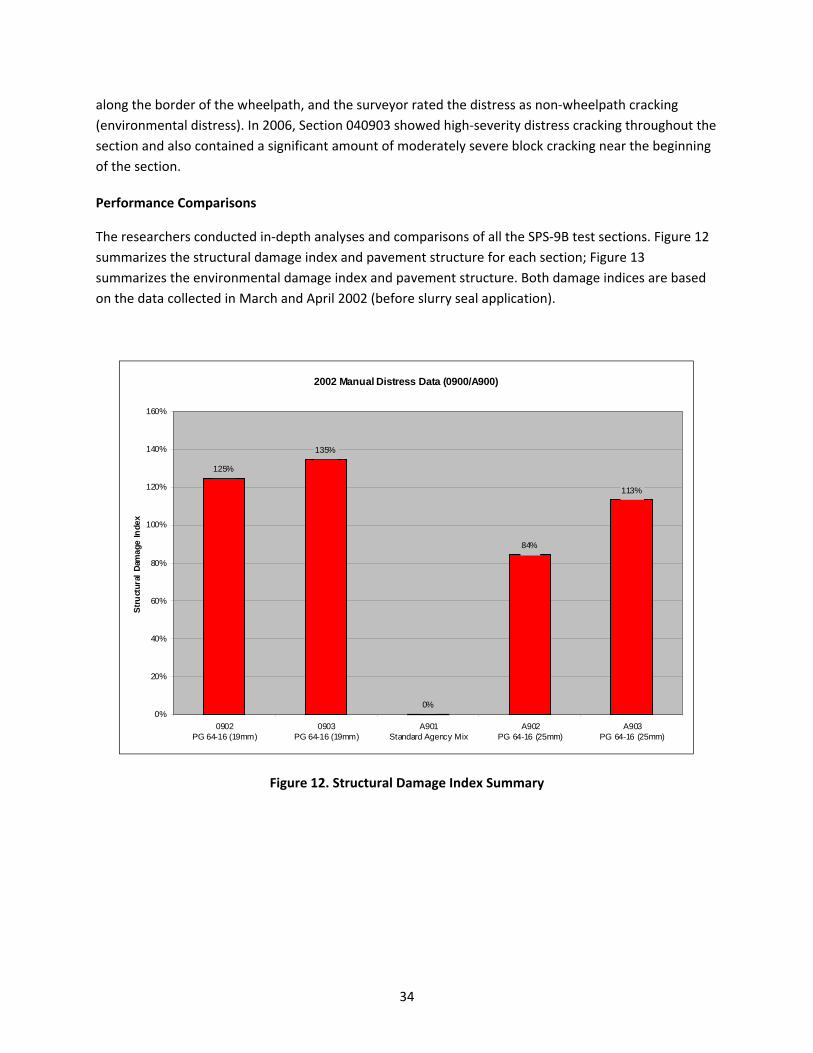
Performance Comparisons
The researchers conducted in‐depth analyses and comparisons of all the SPS‐9B test sections. Figure 12
summarizes the structural damage index and pavement structure for each section; Figure 13
summarizes the environmental damage index and pavement structure. Both damage indices are based
on the data collected in March and April 2002 (before slurry seal application).
Figure 12. Structural Damage Index Summary
2002 Manual Distress Data (0900/A900)
125%
0%
84%
113%
135%
0%
20%
40%
60%
80%
100%
120%
140%
160%
0902PG 64-16 (19mm)
0903PG 64-16 (19mm)
A901Standard Agency Mix
A902PG 64-16 (25mm)
A903PG 64-16 (25mm)
Str
uct
ural
Dam
age
Inde
x

35
Figure 13. Environmental Damage Index Summary
Figure 14 summarizes the amount of rutting in each section as of March or April 2002. The Superpave
sections experienced higher amounts of rutting than the agency mix section (04A901). Comparing the
performance of the Superpave mixes, Sections 04A902 and 04A903 (25‐mm gradation) performed
slightly better than Sections 040902 and 040903 (19‐mm gradation). However, all sections exhibited less
than 9 mm of rutting after over seven years in service, which is well below the level required to trigger
improvements in most pavement management systems. Therefore, rutting was not the driving factor in
the overall condition of the pavement.
2002 Manual Distress Data (0900/A900)
0%
8%
0%
127%
4%
0%
20%
40%
60%
80%
100%
120%
140%
0902PG 64-16 (19mm)
0903PG 64-16 (19mm)
A901Standard Agency Mix
A902PG 64-16 (25mm)
A903PG 64-16 (25mm)
En
viro
nm
enta
l D
amag
e In
dex

36
Figure 14. Rutting Index Summary
Following is a synopsis of the key findings for each section, including overall pavement performance,
structural deterioration, environmental deterioration, rutting, and other unique circumstances.
Section 040902 (Superpave Level 1 Mix, 19‐mm Gradation)
Section 040902 is similar to its replicate, 040903, but 040902 received a slurry seal in 2002. This slurry
seal masked distress and promoted raveling resistance. This section exhibited premature structural
failure and experienced the highest amount of environmental damage. This section experienced the
most rapid increase in environmental distress among all the sections; this occurred from 2002 to 2005.
The researchers attribute this section’s decrease in environmental distress after 2005 to fatigue cracking
spreading outside the wheelpath into existing environmental cracking. This caused cracks that were
rated as environmental cracking in 2005 to be rated as fatigue cracking in 2006.
Section 040903 (Superpave Level 1 Mix, 19‐mm Gradation)
Section 040903 is a replicate of 040902, but unlike 040902, it did not receive any maintenance during
the monitoring period. Like 040902, 040903 experienced premature structural deterioration. In fact, this
section accumulated the most structural damage and the most severe rutting of all the test sections.
However, unlike its counterpart, it experienced significantly less environmental damage (the least of any
2002 Rutting Index (0900/A900)
7.9 7.8
2.2
7.9
6.4
0
1
2
3
4
5
6
7
8
9
0902PG 64-16 (19mm)
0903PG 64-16 (19mm)
A901Standard Agency Mix
A902PG 64-16 (25mm)
A903PG 64-16 (25mm)
Ru
tting
Ind
ex (m
m)

37
section except the agency mix, 04A901). This section also experienced pavement raveling in 2005 and
2006.
Section 04A901 (Standard Agency Mix, 19‐mm Gradation)
The standard agency mix design performed significantly better than all the Superpave sections. Both
structural and environmental deterioration on this section were well below the average for the SPS‐9B
project. Unlike the Superpave sections, this section did not experience pumping, and the amount of
rutting was minimal.
Section 04A902 (Superpave Level 1 Mix, 25‐mm Gradation)
This section exhibited premature structural and environmental deterioration. Section 04A902
experienced the largest amount of environmental distress of all the test sections. This section is similar
to its replicate, 04A903, but 04A902 received a slurry seal in 2002. This slurry seal masked distress and
promoted raveling resistance. However, this section experienced slightly less structural damage and
significantly more environmental damage than its counterpart, 04A903.
Section 04A903 (Superpave Level 1 Mix, 25‐mm Gradation)
Section 04A903 developed the most structural damage of all the test sections. This section is similar to
its replicate, 04A902, but it did not receive any maintenance throughout the monitoring period. This
section experienced slightly more structural damage and significantly less environmental damage than
its counterpart, 04A902. This section also experienced pavement raveling in 2006.
KEY FINDINGS FROM THE SPS‐9B DISTRESS ANALYSIS
The distress data captured at the SPS‐9B project provide valuable insight into pavement performance,
design, management, and construction. Highlights from the SPS‐9B distress analysis follow:
Two of the sections received a slurry seal coat in 2002. This masked the distress that developed
early in the pavement life, but did not otherwise provide a significant improvement in
environmental cracking. Replicates that did not receive the slurry seal experienced higher
amounts of raveling.
All Superpave sections experienced premature structural deterioration, showing significant
growth in fatigue and longitudinal cracking within three years after construction (and in some
cases earlier).
The Superpave mix designs did not include any modifiers or anti‐stripping agents, which may
have contributed to their premature failure.
Construction quality can play a major role in performance. All Superpave sections experienced
segregation during construction that was attributed to the coarseness of the mix and to a paver
problem. Segregation was occurring in the windrow during construction and resulted in random
areas of significant surface voids. Additionally, kickback paddles of the paver appeared to be

38
worn, resulting in a segregated area in the middle of each pass. ADOT observed the mat from
the Superpave mixtures to be very rich and “bony.” However, after three months of traffic the
mat appeared less bony and rich, and segregation did not seem to be a problem. Other factors
that may have contributed to the Superpave sections’ performance were the shorter lengths of
the Superpave sections and a possible lack of contractor experience in constructing pavements
using Superpave mixes as compared to the agency standard mix.
All sections except for 04A902 had reasonable patterns of environmental distress growth, with a
clear increase in magnitude approximately 10 years after construction.
Sections constructed with Superpave mixes exhibited the largest accumulations of structural
deterioration.
Superpave sections with a 19‐mm gradation performed slightly worse in terms of structural
damage than those with a 25‐mm gradation after seven years. However, this performance
difference diminished after 11 years.
All sections performed well with regard to rut resistance. In most sections, rutting would not
have triggered a rehabilitation event.
All Superpave sections experienced pumping by 1998.

39
CHAPTER 4. SPS‐9B ROUGHNESS ANALYSIS
This chapter characterizes the surface roughness of the SPS‐9B test sections throughout their service life
and links the observations to records of pavement distress and its development. Investigators collected
road profile measurements at the site about once per year starting with the winter after the site was
opened to traffic. This study analyzed the profiles in detail by calculating their roughness values,
examining the spatial distribution of roughness within them, viewing them with post‐processing filters,
and examining their spectral properties. These analyses provided details about the roughness
characteristics of the road and provided a basis for quantifying and explaining the changes in roughness
with time.
PROFILE DATA SYNCHRONIZATION
Profile data were collected from the entire Arizona SPS‐9B site on 10 dates between 1994 and 2006 (see
Table 14). Each visit took place during a visit to the SPS‐1 site at the same location. (Note that the visit
numbers in Table 14 correspond to visit numbers referenced in a companion report about the SPS‐1 site,
and that some visits to the SPS‐1 site did not produce any profile measurements on SPS‐9B test
sections.) Raw profile data were available for all 10 visits. Each visit produced a minimum of seven
repeat profile measurements.
Table 14. Profile Measurement Visits to the SPS‐9B Site
Visit Date Time Repeats Section 04A901 040902 04A902 040903 04A903
01 Jan. 27, 1994 — 9 02 Feb 27, 1995 12:45 9 03 Jan. 23, 1997 09:54‐12:50 9 04 Apr. 8, 1998 13:50‐15:31 7 05 Dec. 4, 1998 10:40‐12:16 7 06 Nov. 17, 1999 09:26‐11:06 7 07 Dec. 19, 2000 11:26‐13:31 9 09 Feb. 20, 2002 10:41‐14:25 9 11 March 9, 2004 16:18‐16:40 9 11 March 10, 2004 11:29‐13:34 9 13 March 27, 2006 12:43‐16:12 9
DATA EXTRACTION
Researchers extracted profiles of individual test sections directly from the raw measurements for two
reasons. First, profiles were collected in visits 03 through 09 at a 0.98‐inch sample interval and in visits
11 and 13 at a sample interval of about 0.77 inches. These data appeared in the database after the
application of an 11.8‐inch moving average and decimation to a sample interval of 5.91 inches. The raw

40
data contained the more detailed profiles. Second, this study depended on consistency of the profile
starting and ending points with the construction layout and consistency of the section limits with time.
In particular, a previous quality check revealed that some profiles were shifted (Evans and Eltahan
2000).
In visits 02 through 07, 09, 11, and 13, researchers collected measurements from Sections 04A901,
040902, and 04A902 within long profiles that also included SPS‐1 test sections. Sections 040903 and
04A903 were typically covered in a subsequent set of runs on the same date. The exception was visit 11,
when Sections 040903 and 04A903 were measured on the previous day.
The raw data were used to synchronize all of the profiles to each other through their entire history.
Profiles were synchronized using (1) the site layout from the construction report, (2) event markers in
the raw profiles from the start and end of each section, and (3) automated searching for the longitudinal
offset between repeat measurements.
CROSS CORRELATION
Searching for the longitudinal offset between repeat profile measurements that provides the best
agreement between them is a helpful way to refine their synchronization. This can be done by
inspecting filtered profile plots, but it is very time consuming. Visual assessment is also somewhat
subjective when two profiles do not agree well, which is often the case when measurements are made
several years apart. In this study, investigators used an automated procedure rather than visual
inspection to find the longitudinal offset between measurements.
In this procedure, which is based on a customized version of cross correlation (Karamihas 2004), a basis
measurement is designated that is considered to have the correct longitudinal positioning. A candidate
profile is then searched for the longitudinal offset that provides the highest cross correlation to the basis
measurement. A high level of cross correlation requires a good match of profile shape, the location of
isolated rough spots, and overall roughness level. Therefore, the correlation level is often only high
when the two measurements are synchronized. When the optimal offset is found, a profile is extracted
from the candidate measurement with the proper overall length and endpoint positions. For the rest of
this discussion, this process will be referred to as automated synchronization.
For this application, investigators performed cross correlation after the International Roughness Index
(IRI) filter was applied to the profiles rather than using the unfiltered profiles. This helped assign the
proper weighting to relevant profile features. In particular, it increased the weighting of short‐
wavelength roughness that may be linked to pavement distress. This enhanced the effectiveness of the
automated synchronization procedure. The long‐wavelength content within the IRI output helped
ensure that the longitudinal positioning was nearly correct, and the short‐wavelength content allowed
investigators to leverage profile features at isolated rough spots to fine‐tune the positioning.

41
SYNCHRONIZATION
To extract profiles of individual test sections from the raw measurements, investigators:
1. Established a basis measurement for each section using data from visit 06. This was done using
the event markers from a raw measurement. The first repeat measurement of each section was
used for this purpose. Visit 06 was selected because it included event markers near the
expected locations in each test section. Each section was assumed to begin at the appropriate
event marker and continue for 500 ft.
2. Automatically synchronized the other eight repeats from visit 06 to the basis set.
3. Automatically synchronized the measurements from the previous visit to the current basis set.
4. Designated the previous visit as the current visit.
5. Replaced the basis set with a new set of synchronized measurements from the first repeat of
the current visit.
6. Repeated steps 3 through 5 for each visit from visit 05 to visit 01.
Visits 07 through 13 were also synchronized using steps 3 through 6, but going forward in time.
DATA QUALITY SCREENING
Investigators performed data quality screening to select five repeat profile measurements from each
visit to each section. From the group of available runs, investigators selected the five measurements
that exhibited the best agreement with each other. In this case, agreement between any two profile
measurements was judged by cross correlating them after applying the IRI filter (Karamihas 2004). In
this method, the IRI filter is applied to the profiles, and then the output signals are compared rather
than the overall index. High correlation by this method requires that the overall roughness as well as the
details of the profile shape that affect the IRI agree. The IRI filter was applied before correlation in this
case for several reasons:
• Direct correlation of unfiltered profiles places a premium on very long‐wavelength content, but
ignores much of the contribution of short‐wavelength content.
• Correlation of IRI filter output emphasizes profile features in (approximate) proportion to their
effect on the overall roughness.
• Correlation of IRI filter output provides a good trade‐off between emphasizing localized rough
features at distressed areas in the pavement and placing too much weight on the very short‐
duration, narrow features (spikes) that are not likely to agree between measurements. This is
because the IRI filter amplifies short‐wavelength content, but attenuates macrotexture,
megatexture, and spikes.

42
• A relationship has been demonstrated between the cross correlation level of IRI filter output
and the expected agreement in overall IRI (Karamihas 2004).
Note: This method was performed with a special provision for correcting modest longitudinal distance
measurement errors.
Each comparison between profiles produced a single value that summarized their level of agreement.
When nine repeat profile measurements were available, they produced 36 correlation values. Any
subgroup of five measurements could be summarized by averaging the relevant 10 correlation values.
Researchers selected the subgroup that produced the highest average and excluded the other repeats
from most of the analyses discussed in the rest of this report. Since the number of available profiles
ranged from six to nine, the number of measurements that were excluded ranged from one to four.
Tables 15 through 19 list the selected repeats for each visit to each section and the composite
correlation level they produced.
Table 15. Selected Repeats, Section 04A901
Visit Repeat Numbers Composite Correlation
02 2 3 5 7 8 0.845
03 2 3 4 7 8 0.887
04 1 2 3 4 6 0.847
05 1 2 3 6 7 0.876
06 1 2 4 5 6 0.891
07 1 2 7 8 9 0.910
09 1 2 3 4 5 0.909
11 1 3 4 7 9 0.813
13 2 4 6 7 8 0.848
Table 16. Selected Repeats, Section 040902
Visit Repeat Numbers Composite Correlation
01 1 2 5 7 8 0.894
02 2 3 4 5 9 0.936
03 3 4 6 7 8 0.919
04 1 2 3 6 7 0.852
05 1 2 3 5 7 0.923
06 2 3 5 6 7 0.940
07 2 4 5 7 8 0.941
09 3 4 5 8 9 0.928
11 2 3 7 8 9 0.949
13 2 3 4 5 9 0.949
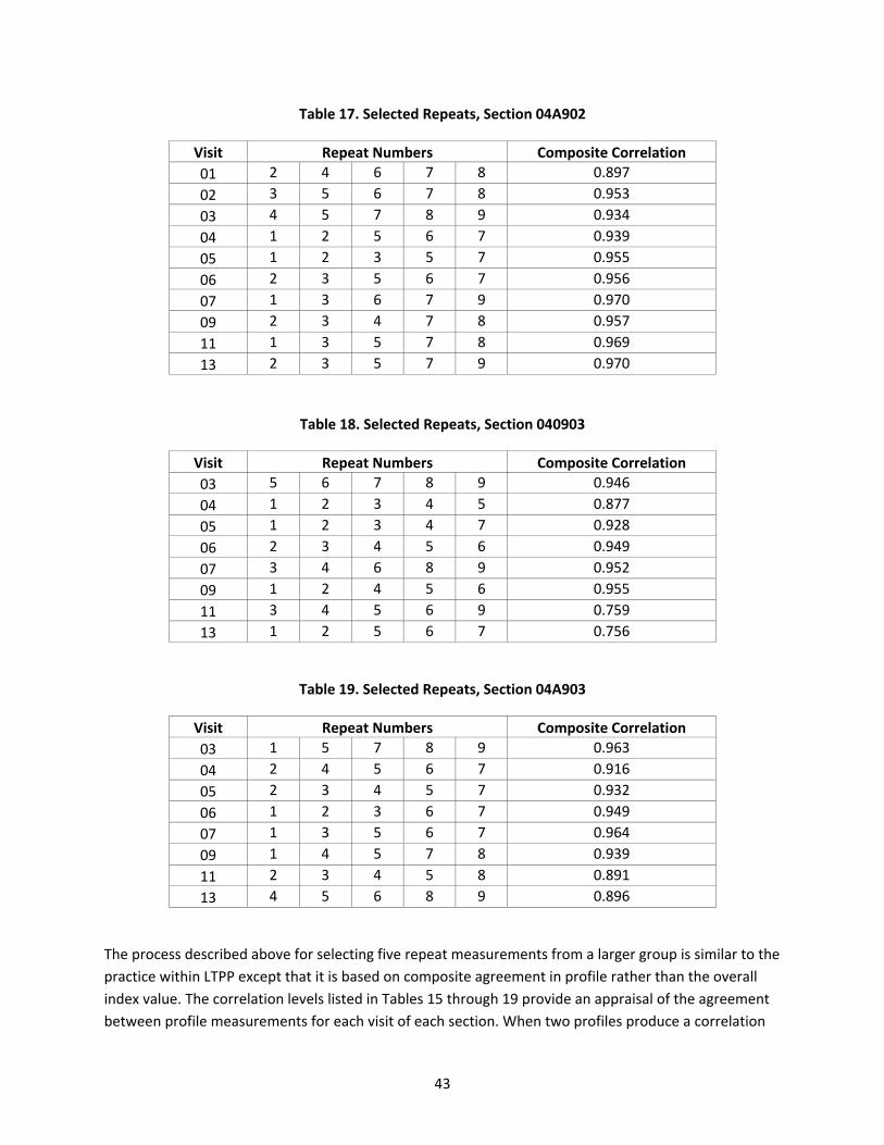
43
Table 17. Selected Repeats, Section 04A902
Visit Repeat Numbers Composite Correlation
01 2 4 6 7 8 0.897
02 3 5 6 7 8 0.953
03 4 5 7 8 9 0.934
04 1 2 5 6 7 0.939
05 1 2 3 5 7 0.955
06 2 3 5 6 7 0.956
07 1 3 6 7 9 0.970
09 2 3 4 7 8 0.957
11 1 3 5 7 8 0.969
13 2 3 5 7 9 0.970
Table 18. Selected Repeats, Section 040903
Visit Repeat Numbers Composite Correlation
03 5 6 7 8 9 0.946
04 1 2 3 4 5 0.877
05 1 2 3 4 7 0.928
06 2 3 4 5 6 0.949
07 3 4 6 8 9 0.952
09 1 2 4 5 6 0.955
11 3 4 5 6 9 0.759
13 1 2 5 6 7 0.756
Table 19. Selected Repeats, Section 04A903
Visit Repeat Numbers Composite Correlation
03 1 5 7 8 9 0.963
04 2 4 5 6 7 0.916
05 2 3 4 5 7 0.932
06 1 2 3 6 7 0.949
07 1 3 5 6 7 0.964
09 1 4 5 7 8 0.939
11 2 3 4 5 8 0.891
13 4 5 6 8 9 0.896
The process described above for selecting five repeat measurements from a larger group is similar to the
practice within LTPP except that it is based on composite agreement in profile rather than the overall
index value. The correlation levels listed in Tables 15 through 19 provide an appraisal of the agreement
between profile measurements for each visit of each section. When two profiles produce a correlation

44
level above 0.82, their IRI values are expected to agree within 10 percent most (95 percent) of the time.
Above this threshold, the agreement between profiles is usually acceptable for studying the influence of
distresses on profile. When two profiles produce a correlation level above 0.92, they are expected to
agree within 5 percent most of the time. Above this threshold, the agreement between profiles is good.
Correlation above 0.92 often depends on consistent lateral tracking of the profiler, and may be very
difficult to achieve on highly distressed surfaces. Note that the IRI values provided in this report are the
average of five observations, which tightens the tolerance even further.
Overall, the majority of the groups of measurements listed in Tables 15 through 19 exhibited good or
better correlation, and most exhibited acceptable correlation. Any group of repeat measurements that
produced a composite correlation level below 0.82 was investigated using filtered plots. These are
discussed below:
Section 04A901, visit 11: Correlation was diminished by sinusoidal chatter in the profiles.
Section 040903, visits 11 and 13: Correlation was significantly diminished by a large number of
narrow downward spikes in the profiles, particularly on the right side.
SUMMARY ROUGHNESS VALUES
Figures 15 through 19 show the left and right IRI values for each pavement section over its monitoring
period. This includes up to 20 summary IRI values (two per visit over up to 10 visits). The figures show
the IRI values versus time in years. In this case, “years” refers from the number of years between the
measurement date and the date the site was opened to traffic, which was August 1, 1993. Fractions of a
year are estimated to the nearest day.
To supplement the plots, the appendix to this report lists the IRI, Half‐car Roughness Index (HRI), and
Ride Number (RN) of each section for each visit. These roughness values are the average of the five
repeat measurements selected in the data quality screening. These are not necessarily the same five
repeat measurements selected for the LTPP database. The appendix also provides the standard
deviation of IRI over the five repeat measurements. This helps identify erratic roughness values that
result from transverse variations in profile caused by surface distresses.
Figures 15 through 19 provide a snapshot of the roughness history of each pavement section. The
remainder of this chapter characterizes the profile content that made up the roughness and explains the
profile features that contributed to roughness progression.

45
Figure 15. IRI Progression, Section 04A901
Figure 16. IRI Progression, Section 040902
0
20
40
60
80
100
120
0 2 4 6 8 10 12 14
RightLeft
Years
IRI (in/mi)
Section A901
0
20
40
60
80
100
120
0 2 4 6 8 10 12 14
RightLeft
Years
IRI (in/mi)
Section 0902

46
Figure 17. IRI Progression, Section 04A902
Figure 18. IRI Progression, Section 040903
0
20
40
60
80
100
120
0 2 4 6 8 10 12 14
RightLeft
Years
IRI (in/mi)
Section A902
0
20
40
60
80
100
120
0 2 4 6 8 10 12 14
RightLeft
Years
IRI (in/mi)
Section 0903

47
Figure 19. IRI Progression, Section 04A903
PROFILE ANALYSIS TOOLS
Investigators used various analysis techniques to study the profile characteristics of each pavement
section and their change with time. These tools help study roughness, roughness distribution, and
roughness progression of each test section, including concentrated roughness that may be linked to
pavement distress. The discussion of each analysis and plotting method is rather brief; Sayers and
Karamihas (1996b) provide more details about these methods.
Roughness Values
Investigators calculated left IRI, right IRI, Mean Roughness Index (MRI), HRI, and RN values. The
appendix to this report provides the average value of each index for each visit of each section. The
discussion of roughness in this analysis emphasizes the left and right IRI. Nevertheless, comparing the
progression of HRI and RN to the MRI provides additional information about the type of roughness that
is changing. For example, a low HRI value relative to MRI indicates roughness that exists on only one side
of the lane. Further, aggressive degradation of RN without a commensurate growth in MRI signifies that
the developing roughness is biased toward short‐wavelength content.
0
20
40
60
80
100
120
0 2 4 6 8 10 12 14
RightLeft
Years
IRI (in/mi)
Section A903
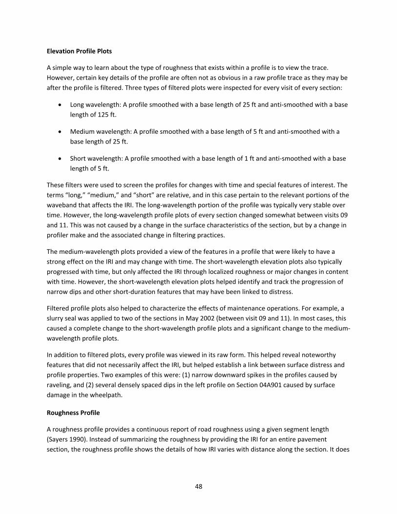
48
Elevation Profile Plots
A simple way to learn about the type of roughness that exists within a profile is to view the trace.
However, certain key details of the profile are often not as obvious in a raw profile trace as they may be
after the profile is filtered. Three types of filtered plots were inspected for every visit of every section:
Long wavelength: A profile smoothed with a base length of 25 ft and anti‐smoothed with a base
length of 125 ft.
Medium wavelength: A profile smoothed with a base length of 5 ft and anti‐smoothed with a
base length of 25 ft.
Short wavelength: A profile smoothed with a base length of 1 ft and anti‐smoothed with a base
length of 5 ft.
These filters were used to screen the profiles for changes with time and special features of interest. The
terms “long,” “medium,” and “short” are relative, and in this case pertain to the relevant portions of the
waveband that affects the IRI. The long‐wavelength portion of the profile was typically very stable over
time. However, the long‐wavelength profile plots of every section changed somewhat between visits 09
and 11. This was not caused by a change in the surface characteristics of the section, but by a change in
profiler make and the associated change in filtering practices.
The medium‐wavelength plots provided a view of the features in a profile that were likely to have a
strong effect on the IRI and may change with time. The short‐wavelength elevation plots also typically
progressed with time, but only affected the IRI through localized roughness or major changes in content
with time. However, the short‐wavelength elevation plots helped identify and track the progression of
narrow dips and other short‐duration features that may have been linked to distress.
Filtered profile plots also helped to characterize the effects of maintenance operations. For example, a
slurry seal was applied to two of the sections in May 2002 (between visit 09 and 11). In most cases, this
caused a complete change to the short‐wavelength profile plots and a significant change to the medium‐
wavelength profile plots.
In addition to filtered plots, every profile was viewed in its raw form. This helped reveal noteworthy
features that did not necessarily affect the IRI, but helped establish a link between surface distress and
profile properties. Two examples of this were: (1) narrow downward spikes in the profiles caused by
raveling, and (2) several densely spaced dips in the left profile on Section 04A901 caused by surface
damage in the wheelpath.
Roughness Profile
A roughness profile provides a continuous report of road roughness using a given segment length
(Sayers 1990). Instead of summarizing the roughness by providing the IRI for an entire pavement
section, the roughness profile shows the details of how IRI varies with distance along the section. It does

49
this by using a sliding window to display the IRI of every possible segment of a given base length along
the pavement.
A roughness profile displays the spatial distribution of roughness within a pavement section. As such, it
can be used to distinguish road sections with uniform roughness from sections with roughness levels
that change over their length. Further, the roughness profile can pinpoint locations with concentrated
roughness and estimate the contribution of a given road disturbance to the overall IRI.
In this work, roughness profiles were generated and viewed using a base length of 25 ft. That means
that every point in the plot shows the IRI of a 25‐ft‐long segment of road, starting 12.5 ft upstream and
ending 12.5 ft downstream. Any location where a peak occurs in the roughness profile that is greater
than or equal to 2.5 times the average IRI for the entire section is considered an area of localized
roughness. All areas of localized roughness are discussed in the detailed observations by identifying
them, listing their severity, and describing the underlying profile features that caused them.
Power Spectral Density Plots
A power spectral density (PSD) plot of an elevation profile shows the distribution of its content within
each waveband. An elevation profile PSD is displayed as mean square elevation versus wave number,
which is the inverse of wavelength. PSD plots were calculated from the slope profile rather than the
elevation profile, which aided in the interpretation of the plots because the content of a slope PSD
typically covers fewer orders of magnitude than an elevation PSD.
A PSD plot is generated by performing a Fourier transform on a profile (or in this case, a slope profile).
The value of the PSD in each waveband is derived from the Fourier coefficients and represents the
contribution to the overall mean square of the profile in that band.
The slope PSD plots provided a very useful breakdown of the content within a profile. In particular, the
plots reveal (1) cases in which significant roughness is concentrated within a given waveband; (2) the
type of content that dominates the profile (e.g., long, medium, or short wavelength); (3) the type of
roughness that increases with time; and (4) the type of roughness that is stable with time.
For the SPS‐9B project, the PSDs rarely provided much value beyond what was learned using filtered
elevation plots and roughness profiles. However, any valuable observations that could be made from
PSD plots are discussed in the following section.
Distress Surveys and Maintenance Records
Once the analysis and plotting were completed, all of the observations were compared to the manual
distress surveys performed on each section. Manual distress survey results were available for each
section on six dates over the monitoring history starting in February 1995. The surveys were performed
using LTPP protocols by technicians certified to perform distress surveys. The surveys provided a means
of relating profile features to known distresses.

50
Researchers also compared observations of changes in profile properties to maintenance records. In
particular, crack sealing affected the presence and shape of narrow dips in one section, and the
application of a slurry seal affected the short‐ and medium‐wavelength content within the profiles on
two sections.
DETAILED OBSERVATIONS
This section reports key observations from the roughness index progression, PSD plots, filtered elevation
profile plots, roughness profiles, and distress surveys. In many cases, similar behavior was noted for
multiple sections. These observations are repeated in each section where appropriate. However,
changes in profile properties with time that were caused by changes in profiler make or model are not
discussed here. These observations are summarized at the end of the report.
Section 04A901, Right Side
Roughness
The IRI increased steadily from 42 to 53 inches/mi over visits 02 through 13.
Elevation Profile Plots
The short‐, medium‐, and long‐wavelength elevation profile plots were very consistent throughout the
monitoring period, with the exception of the area from 360 to 430 ft from the start of the section. In this
area, the medium‐wavelength profile plots changed significantly with each visit. In all visits, a bump over
0.4 inches high appears from 360 to 410 ft from the start of the section. The transitions into and out of
the bump became harsher (i.e., sharper) with time.
Roughness Profiles
Profiles changed very little with time over the first 360 ft of the section. In the last 140 ft of the section,
the roughness increased aggressively with time, and by visit 13 the area centered 413 ft from the start
of the section qualified as localized roughness. The localized roughness there was caused by the trailing
end of the long bump, and had become a sharp slope break by visit 13.
Distress and Maintenance History
Very little distress was recorded for this section, even in later visits.
Section 04A901, Left Side
Roughness
The IRI increased steadily from 35 to 53 inches/mi over visits 02 through 13.
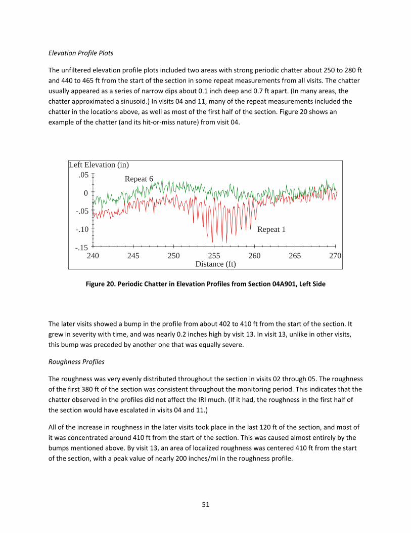
51
Elevation Profile Plots
The unfiltered elevation profile plots included two areas with strong periodic chatter about 250 to 280 ft
and 440 to 465 ft from the start of the section in some repeat measurements from all visits. The chatter
usually appeared as a series of narrow dips about 0.1 inch deep and 0.7 ft apart. (In many areas, the
chatter approximated a sinusoid.) In visits 04 and 11, many of the repeat measurements included the
chatter in the locations above, as well as most of the first half of the section. Figure 20 shows an
example of the chatter (and its hit‐or‐miss nature) from visit 04.
Figure 20. Periodic Chatter in Elevation Profiles from Section 04A901, Left Side
The later visits showed a bump in the profile from about 402 to 410 ft from the start of the section. It
grew in severity with time, and was nearly 0.2 inches high by visit 13. In visit 13, unlike in other visits,
this bump was preceded by another one that was equally severe.
Roughness Profiles
The roughness was very evenly distributed throughout the section in visits 02 through 05. The roughness
of the first 380 ft of the section was consistent throughout the monitoring period. This indicates that the
chatter observed in the profiles did not affect the IRI much. (If it had, the roughness in the first half of
the section would have escalated in visits 04 and 11.)
All of the increase in roughness in the later visits took place in the last 120 ft of the section, and most of
it was concentrated around 410 ft from the start of the section. This was caused almost entirely by the
bumps mentioned above. By visit 13, an area of localized roughness was centered 410 ft from the start
of the section, with a peak value of nearly 200 inches/mi in the roughness profile.
Repeat 1
Repeat 6
240 245 250 255 260 265 270Distance (ft)
-.15
-.10
-.05
0
.05Left Elevation (in)
52
PSD Plots
All of the PSD plots included a peak at a wavelength of about 0.6 ft.
Distress and Maintenance History
Very little distress was recorded for this section, even in later visits. Nothing in the distress histories
explains the bump that caused the localized roughness. A large transverse crack was noted in March
2006 that did appear in the visit 13 profiles as a bump about 44 ft from the section start, but it did not
affect the IRI much.
The chatter in the profile corresponds to a narrow scuff that runs along the left wheelpath over most of
the section and runs off to the edge near the end. It is present in the photos and appears as a long series
of indents about a third of the width of the lane edge stripe. (See Figure 21.)
Figure 21. Pavement Scuff in the Left Wheelpath, Section 04A901
Section 040902, Right Side
Roughness
The IRI increased steadily from 50 to 60 inches/mi.
Elevation Profile Plots
Profiles were very consistent throughout visits 01 through 09, with the exception of some developing
roughness in the medium‐wavelength range. The elevation profiles in the medium‐ and short‐

53
wavelength ranges changed significantly between visits 09 and 11, such that the shape and severity of
most features was often totally different between visits. However, the elevation profiles were extremely
consistent in all 10 repeat measurements from visits 11 and 13. In visits 11 and 13, the feature that
stood out most was a bump 0.1 inch high and 6 ft wide from 78 to 84 ft from the start of the section.
Three other small disturbances were found in the short‐wavelength elevation profile plots 162, 208, and
451 ft from the start of the section.
Roughness Profiles
The roughness was distributed evenly across the section in visits 01 through 09, and the roughness
profiles were fairly consistent across those visits. The visit 11 roughness profiles were significantly
different from those of visit 09. Roughness profiles from visits 11 and 13 were very consistent with each
other, and included one area of localized roughness and another area where localized roughness was
developing. The first was at the bump 78 to 84 ft from the start of the section. This caused a peak in the
roughness profile of about 210 inches/mi. The second rough area appeared about 450 ft from the start
of the section, with a peak value of 120 inches/mi.
Distress and Maintenance History
A slurry seal coat was applied in May 2002. This accounts for the major change in medium‐ and short‐
wavelength content between visits 09 and 11. Nothing in the distress surveys explains the localized
roughness found 78 to 84 ft and 450 ft from the start of the section. Distress surveys from April 2005
and March 2006 identified a significant number of cracks that did not appear to add roughness to the
profiles.
Section 040902, Left Side
Roughness
The IRI generally followed an increasing trend from 48 inches/mi at visit 01 to 66 inches/mi at visit 13.
An out‐of‐trend spike in roughness occurred at visit 09, with an IRI value of 74 inches/mi.
Elevation Profile Plots
No rough features stood out in the short‐wavelength roughness plots in visits 01 through 06. In visit 07,
a dip up to 0.4 inches deep and about 0.5 ft long appeared 213.5 ft from the start of the section. It was
not present in any other visit. Visit 09 profiles included several shallow bumps that did not appear in
profiles from visit 07 or 11. The medium‐ and short‐wavelength elevation profile plots were very similar
in all 10 repeats from visits 11 and 13, but those plots were very different from visit 09. In particular, the
short‐wavelength plots were much smoother in visits 11 and 13 than in visit 09.
Roughness Profiles
Roughness was distributed fairly evenly throughout the section in visits 01 through 07, except that the
area from 160 to 260 ft from the start of the section was about twice as rough as the rest. The narrow

54
dip 213.5 ft from the start of the section was not severe enough to produce localized roughness. The
shallow bumps and extra short‐wavelength roughness in visit 09 caused it to be rougher than previous
visits over the last three‐quarters of the section. In visits 11 and 13, some areas of the section were
rougher than others, but no localized roughness was found. The highest peak in the roughness profile
was caused by a rise in pavement elevation of about 0.25 inches over 5 ft of pavement beginning about
61 ft from the start of the section.
Distress and Maintenance History
A slurry seal coat was applied in May 2002. This accounts for the major change in medium‐ and short‐
wavelength content between visits 09 and 11. Nothing in the distress surveys explains the narrow dip
found in visit 07 or the shallow bumps found in visit 09.
Section 04A902, Right Side
Roughness
The IRI increased steadily from 73 to 96 inches/mi in visits 01 through 09, then diminished to about 69
to 70 inches/mi in visits 11 and 13.
Elevation Profile Plots
Profiles were somewhat consistent from visits 01 through 09. The profiles from visits 11 and 13 were
very consistent with each other. However, in the short‐wavelength range they were not at all similar to
profiles from previous visits, and were markedly different in most locations in the medium‐wavelength
range.
Roughness Profiles
The profiles from visits 01 through 09 included severe localized roughness centered about 260 to 265 ft
from the start of the section. This was caused by a sharp change in slope at the bottom of a long, deep
dip (over 100 ft long and more than 1 inch deep). The dip included a high level of short‐wavelength
roughness at and near its lowest point. Overall, the dip caused a peak in the roughness profile of 240 to
280 inches/mi. In visits 11 and 13, the dip caused a much lower level of peak roughness (150 to 160
inches/mi).
The roughness profiles showed that the roughness progressed across most of the section in visits 01
though 09. The roughness profiles also showed that the roughness was not particularly evenly
distributed along the section in visits 11 and 13, with higher roughness found 60 to 100 ft from the start
of the section, about 410 ft from the start of the section, and at the bottom of the long dip described
above.

55
Distress and Maintenance History
A slurry seal coat was applied in May 2002. This accounts for the change in medium‐ and short‐
wavelength content between visits 09 and 11. Crack sealing was performed on this section in May 2001,
but no major changes occurred in the profiles.
Distress surveys from April 2005 and March 2006 show significant transverse cracking, but no strong
effect (e.g., dips) was found in the profiles.
Section 04A902, Left Side
Roughness
The IRI ranged from 73 to 81 inches/mi without an increasing trend. The highest value occurred in visit
04.
Elevation Profile Plots
Profiles were somewhat consistent in visits 01 through 09. The most noteworthy feature of the profiles
was a set of narrow dips that appeared 355 to 400 ft from the start of the section in visits 05 through 09.
These dips were usually well repeated within a given visit, but they did not always appear in the same
place in different visits.
The profiles from visits 11 and 13 were very consistent with each other. However, they were not at all
similar in the short‐wavelength range to profiles from previous visits, and were markedly different in
most locations in the medium‐wavelength range. The profiles from visits 11 and 13 included a bump
about 0.25 inches high and 0.5 ft long that was 87.5 ft from the start of the section, and a bump
0.2 inches high that ranged from 406 to 414 ft from the start of the section. Neither of these features
were found in previous visits.
Roughness Profiles
The profiles from visits 01 through 09 included localized roughness centered about 260 to 265 ft from
the start of the section. This was caused by a sharp change in slope at the bottom of a long, deep dip
(over 100 ft long and more than 1 inch deep). It caused a peak in the roughness profile of 170 to 230
inches/mi.
In visits 11 and 13, the two bumps described above caused peaks in the roughness profile of over
120 inches/mi, but they were not severe enough to be classified as localized roughness. The long dip
that caused localized roughness in visits 01 through 09 was still present, but it was not as severe.
Distress and Maintenance History
A slurry seal coat was applied in May 2002. This accounts for the change in medium‐ and short‐
wavelength content between visits 09 and 11. Nothing in the distress surveys explains the two bumps
56
noted in visits 11 and 13. Crack sealing was performed on this section in May 2001, but no major
changes occurred in the profiles.
Section 040903, Right Side
Roughness
The IRI increased steadily from 58 to 77 inches/mi from visits 03 through 13.
Elevation Profile Plots
Profiles were very consistent throughout visits 03 through 09, with the exception of some developing
roughness in the medium‐wavelength range. Profiles from visits 11 and 13 were also very similar to
previous visits in the long‐ and medium‐wavelength range, and somewhat similar in the short‐
wavelength range. However, unfiltered plots from visits 11 and 13 included a high density of narrow
downward spikes up to 0.3 inches deep that appeared throughout the section. The spikes rarely
appeared in the same location in more than one or two of the repeat measurements.
Roughness Profiles
The roughness was not particularly evenly distributed along the section, but no areas of localized
roughness were found. The growth in roughness was not isolated to one area.
Distress and maintenance history: A very high level of distress was recorded in April 2005 and May 2006.
This includes fatigue with water bleeding and pumping, and raveling along the entire right wheelpath.
Cracking and raveling, which are confirmed by the photos, explain the narrow downward spikes
dispersed throughout the profiles from visits 11 and 13.
Section 040903, Left Side
Roughness
The IRI followed an unusual trend with time. It was 87 inches/mi in visit 03, 96 inches/mi in visit 04,
91 inches/mi in visit 05, and 82 to 85 inches/mi over the rest of the visits.
Elevation Profile Plots
Profiles were fairly consistent across visits 03 through 05. Profile plots in the long‐, medium‐, and short‐
wavelength ranges were very consistent in visits 06 through 13. However, profiles from visits 11 and 13
included narrow downward spikes up to 0.5 inches deep that appeared throughout the section. The
spikes often appeared in the same location in more than one of the repeat measurements. Fewer spikes
appeared in the left side profiles than on the right, and the spikes that did appear often occurred in
more than one repeat measurement. Figure 22 shows the density and shape of the spikes over 100 ft of
the section in visit 13. In some locations, the spikes appear in only one repeat measurement of the five,
but in others the spikes appear in multiple repeats.

57
Repeat 1
300 320 340 360 380 400
Distance (ft)
-.6
-.4
-.2
0
.2
.4
.6
.8
1.2
1.4
1.6
1.8
2.2
2.4
2.6
2.8Left Elevation (in)
2.0
1.0
Repeat 2
Repeat 5
Repeat 6
Repeat 7
data offset vertically for plotting
Figure 22. Narrow Downward Spikes in Elevation Profile, Section 040903, Visit 13
Roughness Profiles
The roughness was not particularly evenly distributed along the section; the middle third was the
roughest. No areas of localized roughness were found. Although visits 03 through 05 were the roughest,
the roughness profiles did not change much over the monitoring period.
PSD Plots
Significant content was isolated near a wavelength of 40 ft.

58
Distress and Maintenance History
A very high level of distress was recorded in April 2005 and May 2006. This includes fatigue with water
bleeding and pumping, and raveling along the entire right wheelpath. Cracking and raveling, which are
confirmed by the photos, explain the narrow downward spikes dispersed throughout the profiles from
visits 11 and 13.
Section 04A903, Right Side
Roughness
The IRI increased from 72 inches/mi in visit 03 to 113 inches/mi in visit 13. In visits 05 through 07, the IRI
held steady at 98 to 99 inches/mi, and in visits 09, 11, and 13, the IRI was stable at 111 to 113 inches/mi.
Elevation Profile Plots
Profiles did not change much over visits 05 through 07. Unfiltered profiles from visits 11 and 13 included
several downward spikes throughout the length of the section that appeared in only one repeat
measurement in some locations, and in up to three repeats in other locations. With the exception of the
spikes, the profiles from visits 09, 11, and 13 were consistent with each other.
Roughness Profiles
Localized roughness was detected about 70 ft from the start of the section, which caused a peak in the
roughness profile of 180 to 240 inches/mi over the monitoring period. The roughness was caused by a
sharp change in slope about 60 ft from the start of the section at the bottom of a long dip.
In visits 03 through 13, the progression in roughness was very evenly distributed along the section (i.e.,
when roughness increased, it increased equally along the section). The roughness profiles from visits 11
and 13 were very similar to those from visit 09. This is because the spikes in the profiles from visits 11
and 13 were not numerous or severe enough to add significant roughness.
Distress and Maintenance History
A very high level of distress was recorded in April 2005 and May 2006. This includes fatigue with water
bleeding and pumping as well as raveling along the entire right wheelpath. Cracking and raveling, which
are confirmed by the photos, explain the narrow downward spikes dispersed throughout the profiles
from visits 11 and 13.
Section 04A903, Left Side
Roughness
The IRI increased steadily from 71 inches/mi in visit 03 to 108 inches/mi in visit 13.

59
Elevation Profile Plots
The medium‐ and long‐wavelength elevation plots were fairly consistent in visits 03 through 07.
However, the short‐wavelength elevation plots became rougher over time, with the greatest increase
between visits 06 and 09.
The unfiltered elevation profile plots revealed several features that affected roughness. In visit 09, a dip
less than 1 ft long and up to 0.5 inches deep appeared 45 ft from the start of the section. The dip was
not detected in visit 11. It was detected in visit 13 in two of the five repeat measurements, where it was
nearly an inch deep. A less severe dip also appeared 57 ft from the start of the section in two of the five
repeat measurements from visit 09.
Profiles from visits 11 and 13 included several downward spikes throughout the length of the section
that were rarely in the same location in more than one repeat measurement.
Roughness Profiles
No localized roughness was found in any visit, although the roughness was not particularly evenly
distributed along the section. The growth in roughness was not confined to any particular area.
Distress and Maintenance History
A very high level of distress was recorded in April 2005 and May 2006. This includes fatigue with water
bleeding and pumping as well as raveling along the entire left wheelpath. Cracking and raveling, which
are confirmed by the photos, explain the narrow downward spikes dispersed throughout the profiles
from visits 11 and 13. Nothing in the distress measurements explains the dip 45 ft from the start of the
section.

60
SUMMARY
This section summarizes important observations from each section within the SPS‐9B site. Several of the
observations are common to more than one pavement section. In conjunction with the roughness
progression plots (Figures 15 through 19), this summary provides the essential information about each
pavement section. More detail on the profile properties as well as information about data handling and
data quality control is provided in other chapters of this report.
A slurry seal coat was applied to Sections 040902 and 04A902 in May 2002. In both sections, the seal
coat modified the short‐wavelength content of the profiles significantly. Often, the net result was
temporary smoothing of raveling and of narrow dips that appeared at cracks. In both sections, the
medium‐wavelength content of the profiles was also altered. This usually meant that high and low
points within the medium‐wavelength profile plots occurred in roughly the same places, but with
altered shape and severity.
The slurry seal coat reduced the IRI in both sections. The change was largest on the right side of Section
04A902, where the IRI decreased by 27 inches/mi. The change occurred because the right‐side profiles
often included a higher level of narrow dips caused by cracking, which were smoothed out by the seal
coat.
Placement of the seal coat also improved the relationship between the right and left profiles by
eliminating narrow dips and uncorrelated short‐wavelength content. This is demonstrated by the fact
that the difference between the HRI and MRI decreased from 27 percent to 14 percent in Section
040902 and from 25 percent to 10 percent in Section 04A902.
Profiles from Sections 040903 and 04A903 in visits 11 and 13 included several downward spikes that
often appeared in only one or two repeat measurements of each location. These were caused by
cracking and raveling, which covered both wheelpaths; the spikes were more prevalent in the right
wheelpath. The spikes did not affect the IRI significantly.
Significant raveling was also recorded in both sections from visit 09 onward, but the visit 09 profiles did
not include the downward spikes. The explanation may be the change in profiler height sensor footprint
between visits 09 and 11 (Perera and Kohn 2005). In visits 11 and 13, researchers used an International
Cybernetics Corporation MDR 4086L3 profiler. This profiler’s height sensor had a footprint about 1.5 mm
in diameter. In visits 03 through 09, researchers used a K.J. Law Engineers T‐6600 profiler, which had a
height sensor with a footprint that was 38 mm wide and 6 mm long.
The change in profiler in late 2002 affected the long‐wavelength content of the profiles on every test
section. This is because the newer profiler used a high‐pass filter that eliminated a little more of the
profile content than the previous device. The change had no probable effect on the measurement of
localized roughness or the study of narrow bumps and dips caused by distress. However, it did confound
the study of the true effect of the slurry seal coat, since the device change and application of the seal
coat both occurred between visits 09 and 11.

61
Another minor device effect within the profiles was peaks in the PSD plots with no pavement‐related
explanation. In visits 01 and 02 (measured by the K.J. Law DNC 690), most PSD plots from the left side
included a strong peak at a wavelength of 2.5 ft. In visits 03 through 09 (measured by the K.J. Law T‐
6600), all profiles from the left and right sides included a peak in their spectral content at a wavelength
somewhere between 0.35 and 0.65 ft and another at a wavelength of double the first.
Individual Test Sections
The summaries below provide the most important observations made about each test section. To help
provide context for these summary statements, Figure 23 shows the range of left and right IRI for each
section. Note that the highest IRI value for some of the sections did not occur in the final visit. (See the
appendix or Figures 15 through 19.)
Figure 23. Summary of IRI Ranges
Section 04A901
The left side profiles in this section included two patches of sinusoidal chatter in all visits, and included
chatter over the first half of the section in visits 04 and 11. This affected the look of the profiles
0 20 40 60 80 100 120IRI (in/mi)
A901 LR
A902 L
0903
A903
0902
L
L
L
R
R
R
R

62
tremendously, but it did not affect the IRI much. A bump appeared about 400 ft from the start of the
section that became rougher with time, causing localized roughness by visit 13.
Section 040902
The short‐ and medium‐wavelength roughness in this section was altered by the application of a slurry
seal coat in May 2002, which significantly reduced the roughness of the right side. Localized roughness
was found on the right side in visits 11 and 13 at a bump 0.1 inch high from 78 to 84 ft from the start of
the section. A severe narrow dip 0.5 ft long and 0.4 inch deep was found 213.5 ft from the start of the
section in visit 07 only. No corresponding distress was noted.
Section 04A902
The short‐ and medium‐wavelength roughness in this section was altered by the application of a slurry
seal coat in May 2002, which significantly reduced the roughness of the right side. A long, deep dip from
about 205 to 320 ft from the start of the section increased the roughness of the section significantly. The
increase in roughness appeared on both sides, but it was much harsher in the right side profiles. The
feature that affected the roughness most was the change in slope at the deepest part of the dip, and the
short‐wavelength roughness there. The dip registered a much lower level of concentrated roughness on
the right side after the seal coat.
Section 040903
This section showed significant signs of fatigue over the entire pavement surface by the end of the
monitoring period. The profiles from visits 11 and 13 included a large number of narrow downward
spikes caused by cracking and raveling. The location and severity of the spikes was not well correlated
between repeat measurements. No localized roughness was found in this section.
Section 04A903
This section showed significant signs of fatigue over the entire pavement surface by the end of the
monitoring period. The profiles from visits 11 and 13 included a large number of narrow downward
spikes caused by cracking and raveling. The location and severity of the spikes was not well correlated
between repeat measurements. Localized roughness was detected about 70 ft from the start of the
section because of a sharp change in slope at the bottom of a long dip centered 10 ft upstream.

63
CHAPTER 5. CONCLUSIONS AND RECOMMENDATIONS
ADOT initiated the SPS‐9B project to study the relative performance of the Superpave mix designs for
asphalt pavements compared to the agency standard mix design, which will provide a foundation for
future design decisions. While it was found that the agency standard mix design had better performance
in terms of both structural cracking and smoothness, it should be recognized that Superpave mix designs
and construction practices have evolved over the past two decades. (In addition, site‐specific conditions
and construction issues may have negatively affected the performance of the Superpave mixes in this
study.) Surface distress, deflection, and profile data were used as the basis for performance evaluation
and were analyzed as part of the study.
The SPS‐9B project offers a unique opportunity to directly compare performance of various mix designs
while reducing the confounding effect of other variables such as traffic loading, climate, and subgrade
conditions. Conclusions drawn from this comparison are based on one set of in situ conditions;
observations from other climate or loading scenarios may differ from those in this report. Additionally,
the Superpave traffic design and the segregation experienced during the construction of the Superpave
sections may have significantly impacted performance, and the contribution of these factors could not
be fully isolated in the analysis. Therefore, this study’s findings may be unique to the conditions and
construction of this site.
Despite these issues, the data captured at the project provide valuable insight into pavement
performance, design, management, and construction. Following is a summary of lessons learned from
the performance data collected at the SPS‐9B site:
Roughness and roughness progression alone cannot be used to represent the health of a test
section. Several test sections did not exhibit changes in roughness in proportion to the amount
of fatigue cracking, and sections that had clearly reached the end of their service lives did not
necessarily have roughness values that would trigger a rehabilitation event.
In 2002 two test sections received a slurry seal coat, which altered the profile features
significantly and reduced the IRI values. The seal coat masked the distress that began early in
the pavement life, but it did not otherwise significantly improve environmental cracking.
Replicates that did not receive the slurry seal experienced higher amounts of raveling.
Placement of the seal coat improved the relationship between the right‐ and left‐side profiles by
eliminating narrow dips and uncorrelated short‐wavelength content.
All Superpave sections experienced premature structural deterioration, showing significant
growth in fatigue and longitudinal cracking within three years after construction and in some
cases even earlier. Prompted by the overwhelming presence of fatigue, water bleeding, and
pumping, staff from ADOT, FHWA, and Nichols Consulting Engineers conducted a field review of
these sections in 1998. The initial conclusion was that the Superpave sections developed
premature cracking due to stripping of the asphalt concrete (Sebaaly et al. 2001).

64
The Superpave mix designs did not include any modifiers or anti‐stripping agents, which may
have contributed to their premature failure.
Construction quality can play a major role in performance. All Superpave sections experienced
segregation during construction that was attributed to the coarseness of the mix and to a paver
problem. Other factors that may have contributed to the Superpave sections’ performance
included shorter‐length Superpave sections and a possible lack of contractor experience with
using Superpave mixes as compared to the agency standard mix.
All sections except for 04A902 had reasonable patterns of environmental distress growth, with a
clear increase in magnitude approximately 10 years after construction.
Sections constructed with Superpave mixes exhibited the largest accumulations of structural
deterioration.
The agency standard mix (04A901) performed the best both in terms of structural cracking and
smoothness.
Superpave sections with a 19‐mm gradation performed slightly worse in terms of structural
damage than those with a 25‐mm gradation after seven years, but this difference in
performance diminished after 11 years.
All sections performed well with regard to rut resistance. In most sections, rutting would not
have triggered a rehabilitation event.
All Superpave sections experienced pumping by 1998.
A change in profiler equipment or profiler height sensor footprint can greatly affect roughness
data. A profiler change during the test period may have disguised raveling.
Based on these findings, the research team makes the following recommendations:
Site‐specific conditions related to design traffic level and construction issues may have
negatively influenced the performance of the test sections constructed with Superpave mixes.
Therefore, it is important to investigate the performance of other Superpave mixes to obtain a
better understanding of Superpave performance.
The timing of maintenance treatments such as slurry seals should be studied further to
determine the optimum timing to slow environmental deterioration of the pavement.
Most of the pavement test sections appeared to have experienced top‐down cracking, but this
could not be confirmed. It is recommended that forensic analysis be performed at other
locations throughout Arizona to learn about the factors contributing to top‐down cracking.

65
REFERENCES
American Association of State Highway and Transportation Officials (AASHTO). 1993. AASHTO Guide for
Design of Pavement Structures. Washington, D.C.: American Association of State Highway and
Transportation Officials.
Evans, L. D. and A. Eltahan. 2000. LTPP Profile Variability. Publication FHWA‐RD‐00‐113. McLean, VA:
Federal Highway Administration.
Huang, Y. H. 1993. Pavement Analysis and Design. Englewood Cliffs, NJ: Prentice‐Hall.
Karamihas, S. M. 2004. “Development of Cross Correlation for Objective Comparison of Profiles.”
International Journal of Vehicle Design 36(2/3): 173–193.
Karamihas, S. M., T. D. Gillespie, and S. M. Riley. 1995. “Axle Tramp Contribution to the Dynamic Wheel
Loads of a Heavy Truck.” Proceedings of the 4th International Symposium on Heavy Vehicle Weights
and Dimensions, Ann Arbor, MI. C. B. Winkler (ed.): 425–434.
Kim, Y. R., B. Underwood, M. Sakhaei Far, N. Jackson, and J. Puccinelli. 2011. LTPP Computed Parameter:
Dynamic Modulus. Publication FHWA‐HRT‐10‐035. Washington, D.C.: Federal Highway
Administration.
LaCroix, A. T., Y. R. Kim, and S. R. Ranjithan. 2008. “Backcalculation of Dynamic Modulus from Resilient
Modulus of Asphalt Concrete with an Artificial Neural Network.” Transportation Research Record:
Journal of the Transportation Research Board 2057: 107–113.
Mahoney, J. 1995. WSDOT Pavement Guide, Volume 2: Pavement Notes. Olympia: Washington State
Department of Transportation.
Miller, J. S. and W. Y. Bellinger. 2003. Distress Identification Manual for the Long‐Term Pavement
Performance Program. Revised fourth edition. Publication FHWA‐RD‐03‐031. Washington, D.C.:
Federal Highway Administration.
Nichols Consulting Engineers, Chtd. 1997. Arizona SPS‐9P: Construction Report on Site 040900/04A900.
Federal Highway Administration.
Perera, R. W. and S. D. Kohn. 2005. Quantification of Smoothness Index Differences Related to Long‐
Term Pavement Performance Equipment Type. Publication FHWA‐HRT‐05‐054. McLean, VA: Federal
Highway Administration.
Puccinelli, J., S. Karamihas, K. Hall, and K. Senn. 2012. Performance Evaluation of Arizona’s LTPP SPS‐1
Project: Strategic Study of Flexible Pavement Structural Factors. FHWA‐AZ‐12‐396. Phoenix: Arizona
Department of Transportation.

66
Rada, G. R., C. L. Wu, R. K. Bhandari, A. R. Shekharan, G. E. Elkins, and J. S. Miller. 1999. Study of LTPP
Distress Data Variability, Volume I. Publication FHWA‐RD‐99‐074. Washington, D.C.: Federal
Highway Administration.
Sayers, M. W. 1989. “Two Quarter‐Car Models for Defining Road Roughness: IRI and HRI.”
Transportation Research Record: Journal of the Transportation Research Board 1215: 165–172.
Sayers, M. W. 1990. “Profiles of Roughness.” Transportation Research Record: Journal of the
Transportation Research Board 1260: 106–111.
Sayers, M. W. and S. M. Karamihas. 1996a. “Estimation of Rideability by Analyzing Longitudinal Road
Profile.” Transportation Research Record: Journal of the Transportation Research Board 1536: 110–
116.
Sayers, M. W. and S. M. Karamihas. 1996b. Interpretation of Road Roughness Profile Data. Publication
FHWA‐RD‐96‐101 Washington, D.C.: Federal Highway Administration.
Sebaaly, P. E., Z. Eid, and J. A. Epps. 2001. Evaluation of Moisture Sensitivity Properties of ADOT Mixtures
on US 93. FHWA‐AZ98‐402‐01. Phoenix: Arizona Department of Transportation.

67
APPENDIX: ROUGHNESS VALUES
This appendix lists the left International Roughness Index (IRI), right IRI, mean roughness index (MRI),
Half‐car Roughness Index (HRI), and Ride Number (RN) values for each visit of each section. The
roughness values are the average for five repeat runs. The five runs were selected from a group of as
many as nine by automated comparison of profiles, as described in the report. Values of standard
deviation are also provided for left and right IRI to reveal cases of high variability among the five
measurements. However, the screening procedure used to select five repeats usually helped reduce the
level of scatter.
The discussion of roughness in the report emphasizes the left and right IRI. Nevertheless, the other
indexes do provide useful additional information. MRI is simply the average of the left and right IRI
values. HRI is calculated by converting the IRI filter into a half‐car model (Sayers 1989) by collapsing the
left and right profiles into a single profile in which each point is the average of the corresponding left
and right elevations. The IRI filter is then applied to the resulting signal. The HRI is very similar to the IRI
except that side‐to‐side deviations in profile are eliminated. The result is that the HRI value for a pair of
profiles will always be lower than the corresponding MRI value. Comparing the HRI and MRI values
provides a crude indication of the significance of roll (i.e., side‐to‐side profile variation) in the overall
roughness measurement. When HRI is much lower than MRI, roll is significant. This is common among
asphalt pavements (Karamihas et al. 1995). Certain types of pavement distress, such as longitudinal
cracking, may also cause significant differences between HRI and MRI.
Figure 24 compares the HRI and MRI for all of the profile measurements that are covered in this
appendix (225 pairs of roughness values). The figure shows a best fit line with a zero intercept and a line
of equality. The slope of the line is 0.773. This is an unusually large difference between HRI and MRI.
Note that a better linear fit was found without forcing a zero intercept. A simple linear fit produced a
slope of about 0.711 and an intercept of about 4.6 inches/mi.
RN has shown a closer relationship to road user opinion than the other indexes (Sayers and Karamihas
1996a). As such, it may help distinguish the segments from each other by ride quality. Further, the effect
on RN may help quantify the impact of that distress on ride when a particular type of distress dominates
the roughness of a section. In particular, a very low RN value coupled with moderate IRI values indicates
a high level of short‐wavelength roughness and potential sensitivity to narrow dips and measurement
errors caused by coarse surface texture.
Table 20 provides the roughness values. The table also lists the date of each measurement and the time
in years since the site was opened to traffic. Negative values indicate measurements that were made
before rehabilitation.

68
Figure 24. Comparison of HRI to MRI
Table 20. Roughness Values
Section Date Years
Left IRI (inches/mi)
Right IRI (inches/mi)
MRI (inch/mi)
HRI (inch/mi)
RN Avg.
St. Dev.
Avg. St. Dev.
040902
27‐Jan‐94 0.49 48 1.0 50 0.6 49 39 4.05 27‐Feb‐95 1.57 50 0.9 50 0.6 50 40 4.10 23‐Jan‐97 3.48 53 0.6 53 0.3 53 41 3.96 8‐Apr‐98 4.68 62 2.9 55 1.3 59 43 3.70 4‐Dec‐98 5.34 57 0.8 54 1.3 56 41 3.77 17‐Nov‐99 6.29 59 0.7 56 0.5 57 43 3.84 19‐Dec‐00 7.38 59 0.9 55 0.3 57 43 3.77 20‐Feb‐02 8.56 74 0.9 59 1.0 66 48 3.50 10‐Mar‐04 10.61 67 0.7 59 1.0 63 54 3.75 27‐Mar‐06 12.65 66 0.5 60 1.2 63 54 3.75
040903
23‐Jan‐97 3.48 87 0.9 58 0.4 73 57 3.85 8‐Apr‐98 4.68 96 3.0 63 0.5 79 61 3.48 4‐Dec‐98 5.34 91 1.0 61 0.6 76 59 3.58 17‐Nov‐99 6.29 84 0.9 64 0.7 74 58 3.65 19‐Dec‐00 7.38 82 0.4 64 0.7 73 58 3.61 20‐Feb‐02 8.56 82 0.3 69 0.9 75 59 3.42 9‐Mar‐04 10.60 83 2.3 73 2.8 78 60 3.13 27‐Mar‐06 12.65 85 3.2 77 2.2 81 63 2.95
0
20
40
60
80
100
120
0 20 40 60 80 100 120
HRI = 0.773•MRI
Line of Equality
HRI (in/mi)
MRI (in/mi)

69
Table 20. Roughness Values (cont.)
Section Date Years
Left IRI (inches/mi)
Right IRI (inches/mi)
MRI (inch/mi)
HRI (inch/mi)
RN Avg.
St. Dev.
Avg. St. Dev.
04A901
27‐Feb‐95 1.57 35 1.6 42 0.7 38 31 4.27 23‐Jan‐97 3.48 37 0.4 46 0.6 41 32 4.23 8‐Apr‐98 4.68 37 0.7 49 0.3 43 34 4.10 4‐Dec‐98 5.34 37 0.6 48 0.4 43 34 4.16 17‐Nov‐99 6.29 40 0.6 47 1.1 44 35 4.17 19‐Dec‐00 7.38 38 0.9 48 0.3 43 34 4.24 20‐Feb‐02 8.56 43 0.8 48 0.3 45 37 4.16 10‐Mar‐04 10.61 43 0.7 48 1.0 45 37 3.98 27‐Mar‐06 12.65 53 0.9 53 0.7 53 43 3.80
04A902
27‐Jan‐94 0.49 73 1.1 73 1.0 73 60 3.70 27‐Feb‐95 1.57 74 1.1 77 0.9 76 60 3.75 23‐Jan‐97 3.48 76 2.0 82 1.7 79 61 3.65 8‐Apr‐98 4.68 81 2.1 89 1.4 85 64 3.39 4‐Dec‐98 5.34 72 0.5 88 1.8 80 60 3.57 17‐Nov‐99 6.29 75 1.6 90 1.3 83 64 3.52 19‐Dec‐00 7.38 75 0.6 92 1.1 84 65 3.51 20‐Feb‐02 8.56 79 0.8 96 1.1 87 66 3.45 10‐Mar‐04 10.61 75 0.1 69 0.8 72 65 3.76 27‐Mar‐06 12.65 75 0.9 70 0.4 73 65 3.75
04A903
23‐Jan‐97 3.48 71 0.7 72 0.6 71 54 3.73 8‐Apr‐98 4.68 78 1.5 85 1.9 82 62 3.38 4‐Dec‐98 5.34 82 1.4 98 2.5 90 69 3.34 17‐Nov‐99 6.29 90 1.5 98 1.9 94 69 3.36 19‐Dec‐00 7.38 92 1.2 99 1.1 96 70 3.31 20‐Feb‐02 8.56 101 1.1 111 1.5 106 77 2.99 9‐Mar‐04 10.60 98 2.9 111 1.7 105 78 2.90 27‐Mar‐06 12.65 108 1.1 113 1.3 111 81 2.71

70