The Journal of Futures Markets, Vol. 18, No. 5, 487–517 (1998)Q 1998 by John Wiley & Sons, Inc. CCC 0270-7314/98/050487-31

Spread Options,Exchange Options, and

Arithmetic Brownian

Motion

GEOFFREY POITRAS*

INTRODUCTION

Since the early contributions of Black and Scholes (1973) and Merton(1973), the study of option pricing has advanced considerably. Much ofthis progress has been achieved by retaining the assumption that therelevant state variable follows a geometric Brownian motion. Limitationsinherent in using this assumption for many option pricing problems haveled to theoretical extensions involving the introduction of an additionalstate variable process.1 Except in special cases, the presence of this ad-ditional process requires a double integral to be evaluated to solve theexpectation associated with the option valuation problem. This compli-cates the European option pricing problem to the point where a closedform is usually not available and numerical techniques are required tosolve for the option price. Such complications arise in the pricing ofspread options (see Shimko, 1994; Pearson, 1995), options which havea payoff function depending on the difference between two prices and an

This article was written while the author was a Senior Fellow in the Department of Economics andStatistics, National University of Singapore (NUS). Helpful comments were received from JohnHeaney, Christian Wolff, Tse Yiu Kuen, and Lim Boon Tiong as well as from seminar participantsat NUS. The insightful comments of two anonymous referees are also gratefully acknowledged.*For correspondence, Faculty of Business Administration, Simon Fraser University, Burnaby, BritishColumbia, Canada V5A 1S6.1Examples include many of the exotic options as well as the stochastic convenience yield and sto-chastic volatility models (e.g., Rubinstein, 1991a,b; Gibson and Schwartz, 1990; Ball and Roma,1994).

■ Geoffrey Poitras is a Professor at Simon Fraser University.

488 Poitras

exercise value. For lognormally distributed state variables, a closed formfor the spread option price is only available for the special case of anexchange option or, more precisely, an option to exchange one asset foranother (Margrabe, 1978; Carr, 1988; Fu, 1996).2

The objective of this article is to develop pricing formulae for Eu-ropean spread options under the assumption that the prices follow arith-metic Brownian motions.3 Significantly, unlike the lognormal case, as-suming arithmetic Brownian motion does permit the derivation of simpleclosed forms for spread option prices. The potential generality of assum-ing arithmetic Brownian motion for single state variable option pricingproblems has been demonstrated by Goldenberg (1991), who providesvarious option pricing results derived using arithmetic Brownian motionwith an absorbing barrier at zero. Due to the complexities of using ab-sorbed Brownian motion for pricing spread options, this article arguesthat assuming arithmetic Brownian motion without an absorbing barrierat zero is appropriate for developing spread option pricing results. Theresulting option price is a special case of a Bachelier option, an optionprice derived under the assumption of unrestricted arithmetic Brownianmotion.4 In this vein, Bachelier exchange option prices can be contrastedwith the Black-Scholes exchange option to benchmark relative pricingperformance. Even though the homogeneity property used to simplify thelognormal case does not apply to the Bachelier exchange option, the li-nearity property of arithmetic Brownian motion provides for a similarsimplification.

The following section reviews previous studies which have assumedarithmetic Brownian motion to derive an option pricing formula. Argu-ments related to using this assumption in pricing spread options are re-viewed. The second section provides European spread option priceswhere the individual security prices are assumed to follow arithmeticBrownian motion. Bachelier spread option prices for assets with equaland unequal proportional dividends, as well as spread options on futurescontracts, are derived. Implications associated with different types ofspread option contract design are also discussed. The third section pres-

2It is also possible to use lognormality to solve the spread option for the redundant case where thespread is treated as a single random variable. While this case is potentially applicable to a range ofspread options, e.g., credit spreads such as the Treasury bill/Eurodollar (TED) spread, this approachis inconsistent with the assumption that the individual prices are lognormally distributed. This followsbecause the difference of lognormal variables will not be lognormal.3This class of processes includes all untransformed prices with diffusions having stationary distri-butions which are normal. Other terminology such as absolute Brownian motion and Gaussian pro-cess is also used.4This terminology follows Smith (1976) and Goldenberg (1991). Austin (1990) associates a Bachelieroption with absorbed Brownian motion.

Spread Options 489

ents results for alternatives to the Bachelier option. It is demonstratedthat the commonly used Wilcox spread option formula does not satisfyabsence-of-arbitrage requirements. Recognizing that the exchange optionis a special type of spread option, closed form solutions are provided forBlack-Scholes exchange options using securities with dividends as wellas for futures contracts. In the fourth section some simulated pricingscenarios are used to identify relevant features of the Bachelier spreadoption and to contrast the properties of Bachelier exchange options withthe Black-Scholes exchange options. Finally, a summary of the main re-sults is presented.

BACKGROUND INFORMATION ANDLITERATURE REVIEW

Despite having received only limited empirical support in numerous dis-tributional studies of financial prices, the analytical advantages of assum-ing geometric Brownian motion have been substantial enough to favorretaining the assumption in theoretical work. While much the same theo-retical advantages can be achieved with arithmetic Brownian motion, thisassumption has been generally avoided. Reasons for selecting geometricrather than arithmetic Brownian motion were advanced at least as earlyas Samuelson (1965) and some of the studies in Cootner (1964). In re-viewing previous objections, Goldenberg (1991) recognizes three whichare of practical importance: (i) a normal process admits the possibility ofnegative values, a result which is seemingly inappropriate when a securityprice is the relevant state variable; (ii) for a sufficiently large time toexpiration, the value of an option based on arithmetic Brownian motionexceeds the underlying security price; and (iii) as a risk-neutral process,arithmetic Brownian motion without drift implies a zero interest rate.Taken together, these three objections are relevant only to an unrestricted“arithmetic Brownian motion” which is defined to have a zero drift. Assuch, some objections to arithmetic Brownian motion are semantic,avoidable if the process is appropriately specified.

Smith (1976) defines arithmetic Brownian motion to be driftless andprovides an option pricing formula which is attributed to Bachelier (1900)and is subject to all of the three objections. Smith (1976, p. 48) arguesthat objection (ii) is due to the possibility of negative sample paths,though this objection can be avoided by imposing an appropriate drift.Goldenberg (1991) reproduces the Smith-Bachelier formula and pro-ceeds to alter the pricing problem by replacing the unrestricted driftlessprocess with an arithmetic Brownian motion which is absorbed at zero.

490 Poitras

The resulting option pricing formula avoids the first two objections. Thethird objection is addressed by setting the drift of the arithmetic Brownianprocess equal to the riskless interest rate times the security price, con-sistent with an Ornstein-Uhlenbeck (OU) process (e.g., Cox and Miller,1965, pp. 225–228). Using this framework, Goldenberg (1991) gener-alizes an option pricing result in Cox and Ross (1976) to allow for chang-ing variances and interest rates. With the use of appropriate transfor-mations for time and scale, Goldenberg (1991) argues that a wide rangeof European option pricing problems involving diffusion price processescan be handled using the absorbed-at-zero arithmetic Brownian motionapproach.

An alternative to using absorbed Brownian motion, adaptable to thestudy of spread options, is to derive the option price formula using un-restricted arithmetic Brownian motion with drift. While this does notaddress objection (i), it can handle the other two. An option pricing modelfor individual securities which uses this approach does appear in Brennan(1979), a study of the utility-theoretic properties of contingent claimsprices in discrete time.5 However, the intuitive limitations of arithmeticBrownian motion associated with objection (i) combined with the avail-ability of simple closed form solutions for absorbed Brownian motionhave created a situation where results on the Bachelier option for indi-vidual securities are generally unavailable. The situation for spread op-tions is somewhat different. Significantly, for the pricing of spread op-tions, assuming that prices follow unrestricted arithmetic Brownianmotions permits the derivation of substantively simpler closed forms thanassuming that the prices forming the spread follow absorbed Brownianmotions. Even though absorbed arithmetic Brownian motion has greaterintuitive appeal due to the avoidance of negative sample paths for theindividual prices, this advantage typically will not be of much practicalrelevance for pricing spread options.

Determining a spread option formula when the prices are assumedto be absorbed Brownian motions is complicated and the resulting theo-retical prices will only differ from the unrestricted case if there is signifi-cant probability of the price processes reaching zero (Heaney and Poitras,1997). Hence, for pricing traded spread options, much of the concernabout price processes being absorbed at zero is moot, because the prob-ability of either process being absorbed is almost zero. For example, con-

5As in Goldenberg (1991) and Smith (1976), Brennan (1979) neglects to make an obvious simplifi-cation in the formula involving the argument entering the cumulative distribution function (cdf ) andprobability density function (pdf ). As indicated in Cox and Ross (1976), the N and n function ar-guments are the same.

Spread Options 491

sider the following candidate variables for spread options: the differencein the price of heating oil and gasoline; the difference in the Nikkei andthe Dow Jones stock price indices; and the difference in the price of goldor copper futures contracts for different delivery dates. The practical like-lihood of any of these price processes going to zero is negligible. While,in general, the validity of the unrestricted Brownian solution will dependon the type of spread being evaluated, cases for which it is not a plausiblecandidate process are difficult to identify in practice. In addition, directevaluation of the spread option assuming lognormally distributed pricesrequires a complicated double-integration over the joint density of S2 andS1, which has to be evaluated numerically. Again, treating the spread asan unrestricted arithmetic Brownian motion has substantive analyticaladvantages.

Without precise empirical information on specific spread distribu-tions, spread options are a security which arguably could provide a usefulapplication of the Bachelier option. This insight was first exploited in atrade publication (see Wilcox, 1990), which employs arithmetic Brownianmotion to derive a closed form spread option pricing formula. However,as demonstrated in the section “Other Types of Spread and ExchangeOptions,” the Wilcox formula is not consistent with absence-of-arbitrageand, as a result, is not a valid option pricing formula. Despite its theo-retical limitations, the Wilcox model has been used as a benchmark pric-ing result in a number of studies. In particular, Shimko (1994) and Pear-son (1995) both compare the Wilcox model with option prices derivedfrom a double-integration approach involving lognormally distributedprices. Pearson (1995) contrasts the performance of the Wilcox spreadoption with a double-integration approach which is analytically simplifiedby providing a closed form solution to the first integration. A numericalalgorithm is used to solve the second integral and arrive at exact prices.Evaluating option prices and delta for a number of specific examples,Pearson (1995) claims that the double-integral lognormal solution pro-vides substantially more accurate pricing than the Wilcox approach, par-ticularly for long maturity options.

Shimko (1994) applies the Jarrow and Rudd (1982) approximationtechnique to the Wilcox (1990) option price to approximate the “true”lognormal solution. In effect, the Wilcox formula is augmented with theaddition of higher order moment terms which approximate the differencebetween the normal and lognormal cases. Indirect information on therelative performance of the Wilcox option is provided in a specific illus-tration of the “accuracy of analytical approximation” (Shimko, 1994, pp.211–212), which contrasts the prices from the approximation and an

492 Poitras

exact double-integral lognormal solution which encompasses stochasticconvenience yield. However, because Shimko (1994) relies on the Wilcoxspread option formula, the comparison between the double lognormalintegration approach and the arithmetic Brownian motion spread optionmodel is not fully developed. In addition, it is not clear to what extentthe limitations of the Wilcox model have been incorporated in the Jarrowand Rudd approximation solution. Finally, Shimko (1994, p. 184) makesan important, if debatable, statement about spread options: “. . . the be-haviour of the spread option is affected by the behaviour of two tradedcontracts; a spread cannot be modelled as if it is a single asset.” This isprecisely what assuming arithmetic Brownian motion permits.

Shimko (1994) recognizes that a fundamental difficulty in evaluatingspread option pricing models is the limited number of traded securities.As a consequence, there are only a limited number of empirical studieson spread options. Grabbe (1995) provides some empirical informationon copper spread options traded on the London Metals Exchange (LME),while Wilcox (1990) examines traded oil spread options and Falloon(1992) provides some practical examples. Despite the presence of thesefew studies, the data on spread options are, at this point, insufficient tosupport conclusions about the superiority of one pricing method overanother. Related empirical evidence on the distribution of spreads is alsolimited. Poitras (1990) provides a detailed study of the distribution ofgold futures spreads, together with a methodology for deconvolving thedistribution into two component distributions. However, because goldtends to be at or near full-carry, the distributional information is of limitedvalue for inferring the distribution of other types of spreads. Gibson andSchwartz (1990) use a time series approach to evaluate the behavior ofconvenience yield for crude oil, providing useful information about thespread distribution for that commodity. Some limited empirical infor-mation is also available in other sources, e.g., Rechner and Poitras (1993)on the soy crush spread.

BACHELIER SPREAD OPTION PRICING6

On the expiration date, the payout on a spread option has the form7:

C 4 max[S 1 S 1 X, 0]T 2T 1T

6Relevant distribution-free properties of spread options including put-call parity conditions are ex-amined in Shimko (1994) and Grabbe (1995). One fundamental result provided by Shimko (1994,p. 191) is that the value of a spread option with exercise price, X, will be less than or equal to anycombination of a call on S2 with exercise price, X2, and a put on S1 with exercise price, X1, given X2

Spread Options 493

where T is the expiration date of the option, CT is the call option priceat time T, X is the exercise value (which can be either positive or negative),and S2T 1 S1T is the difference between two prices, S2 and S1 at time T.The complexity of the spread option pricing problem is reflected in studieswhich have taken the direct approach to valuation (e.g., Shimko, 1994;Pearson, 1995; Ravindran, 1993; Bjerksund and Stensland, 1994;Grabbe, 1995). The direct approach involves solving the risk-neutral valu-ation problem for the European spread option price:

1rt*C 4 e E[max[S 1 S 1 X, 0]] 4t 2T 1T

1rt*e max[S 1 S 1 X, 0] g[S |S ] ƒ [S ] dS dS2T 1T 2,T 1,T 1,T 2 15# # 6where the risk-neutral expectation is taken with respect to a lognormalconditional density, g[•], and marginal density, f[•]. From this point, anumber of solution techniques are available. However, with lognormallydistributed price processes, it is only possible to achieve a closed formsolution in the special case of an exchange option, where one of the assetscan be used as a numeraire. Otherwise, some numerical technique mustbe implemented to evaluate the double integral. In this process, while itis possible to derive a closed form solution to the first integration wherethe expectation is taken with respect to the conditional density, e.g., Pear-son (1995), the second integral must be evaluated numerically.8

One advantage of having a closed form solution is the avoidance ofhaving to numerically evaluate a double integral to determine optionprices. In the absence of traded securities, it is difficult to assess relativepricing performance and, by implication, the validity of a given modelingapproach. Moreover, it is reasonable to assume that the distributionalassumption selected would depend on the specific type of spread beingmodeled. Unlike individual security prices, the spread distribution de-pends on the difference of two, possibly disparate, distributions. In gen-eral, evaluation of the resulting convolution is difficult, though it is pos-sible to conclude that a wide range of distributions can result.9 Given

1 X1 4 X. In effect, a spread option will be less expensive than trading puts and calls on theunderlying commodities in the spread.7This form of the spread option suppresses consideration of the method of specifying units of thesecurities or commodities being exchanged. In many cases, the number of units being exchanged willbe equal and the option price can be considered a per unit price. In other cases, the units beingexchanged will differ and the prices will represent the value of the items being exchanged.8Hybrid approaches are also possible, as in Grabbe (1995) or Shimko (1994). An alternative pricingmethodology is provided by Brooks (1995) which uses a lattice approach to valuing spread options.9For example, the difference or sum of two lognormally distributed distributions will not usually be

494 Poitras

this, arithmetic Brownian motion is one potentially viable candidate pro-cess. Recognizing that the spread option pricing problem will have dif-ferent solutions, depending on the empirical distribution of the spreadbeing modeled, it is in sharp contrast to the current modeling conventionof assuming lognormally distributed prices and treating the spread optionin a general fashion, making limited reference to either potential varia-tions in the design of the spread option or to empirical characteristics ofthe underlying spread. This ignores the possibility that the solution to thespread option pricing problem can differ, depending on the types ofspreads being considered. For example, S2 and S1 could be the prices ofgold contracts for different delivery dates, an intracommodity futuresspread option or the Nikkei and S&P stock indices, or the prices of crudeoil and gasoline.

One possible generic type of price spread occurs where the securitiesboth pay the same proportional dividend (dS dt). If it is assumed that theindividual price processes both follow arithmetic Brownian motion, thenthe price spread will follow the diffusion:

d(S 1 S ) 4 (r 1 d)(S 1 S ) dt ` r dW (1)2 1 2 1 s s

where the drift and volatility parameters are specified to be consistentwith absence-of-arbitrage. This diffusion is constructed by taking S2 andS1 to both follow unrestricted arithmetic Brownian motions of the form:

dS 4 (r 1 d) S dt ` r dW dS 4 (r 1 d) S dt ` r dW2 2 2 2 1 1 1 1

where the variance of the joint process is specified as

2 2 2r 4 r 1 2r ` rS 1 12 2

Hence, as a consequence of assuming that the individual price processesfollow unrestricted arithmetic Brownian motions with appropriately spec-ified coefficients, it is possible to construct a stochastic differential equa-tion (SDE) for the price spread as eq. (1), where the spread can be treatedas a single random variable. Because the difference of lognormal variablesis not lognormal, a similar simplification is not available if the price pro-cesses are assumed to be lognormal.

In what follows, derivation of the closed form solutions for the spreadoption prices proceeds by stating the partial differential equation (PDE)

lognormal, though the product will be. Similarly, while the sum of two exponentially distributedvariables will be gamma, the same is not true about the difference. A key advantage of using normalrandom variables to model spreads is that the convolution of the difference of two normal distribu-tions is also normal.

Spread Options 495

for the dynamic hedging problem and verifying that the stated solutionsatisfies the PDE. The procedure for deriving the PDE is not stated ex-plicitly but does follow the standard procedure of identifying the relevantriskless hedge portfolio, which is composed of a long and a short positionin the commodities or securities determining the spread. This cash po-sition is dynamically hedged by writing an appropriate number of spreadcall options. This riskless hedge portfolio provides two conditions: oneassociated with applying Ito’s lemma and another associated with therestriction that the net investment in the hedge portfolio must earn theriskless rate of interest. Equating these two conditions and manipulatingprovides the PDE associated with the dynamic hedging problem. Thevalidity of the solutions given in the various propositions is proved byevaluating the relevant partial derivatives of the stated option formulaand verifying that the closed form satisfies the PDE. By construction, ifthe PDE is satisfied, the result is consistent with absence-of-arbitrage.

In the special case where both S2 and S1 are assets which pay thesame constant dividend rate (d), the PDE associated with riskless hedgeportfolio problem for the spread option can be motivated by treating thespread as a single random variable and using the well-known PDE for thesingle variable case which gives:

2]C ]C 1 ] C 24 rC 1 (r 1 d) (S 1 S ) 1 r (2)2 1 s21 2]t ](S 1 S ) 2 ](S 1 S )2 1 2 1

By treating the spread as a single random variable, this PDE involves onlyone delta hedge ratio and one gamma. In general, the riskless hedge port-folio for a spread option will involve two delta hedge ratios, one for eachof the two spot (or futures) positions. Evaluating the riskless hedge port-folio for this dynamic hedging problem produces the PDE:

]C ]C ]C4 rC 1 (r 1 d) S ` S1 25 6]t ]S ]S1 2

2 2 21 ] C ] C ] C2 21 r ` 2 r ` r (3)1 12 22 25 62 ]S ]S ]S ]S1 1 2 2

For the arithmetic Brownian diffusion process, the solutions to the PDEs(2) and (3) are equivalent, a result which can be verified by taking therelevant derivatives of the formula given in Proposition I.

496 Poitras

Given this background, it is now possible to provide the followingresult.

Proposition I: The Bachelier Spread Option forEqual Dividend-Paying Securities

Assuming perfect markets and continuous trading, for a price spread in-volving two prices making equal dividend payments and both obeyingarithmetic Brownian motion, the absence-of-arbitrage solution that sat-isfies the PDEs (2) and (3) is the Bachelier spread option pricing formula:

C [S 1 S , t*; r, d, r, X] 4St 2 1

1d 1t* rt*((S 1 S )e 1 Xe ) N[y] ` V n[y] (4)2t 1t

where

t*1d 1 1 1rt* 2 t* 2rt*d(S 1 S )e 1 Xe e 1 e2t 1ty 4 V 4 rS 5 6!V 2(r 1 d)

CSt is the price of the Bachelier spread call option for equal dividend-paying securities, and N[y] and n[y] represent the cumulative normalprobability function and normal density function, respectively, evaluatedat y.

The proof of Proposition I (given in the Appendix) verifies by directdifferentiation that this solution satisfies the PDE for the dynamic hedg-ing problem. In the section “Other Types of Spread and Exchange Op-tions,” it will be verified that eq. (1), the SDE for the spread processassociated with Proposition I, imposes the appropriate absence-of-arbi-trage restriction on the drift coefficient. The special case of securitieswhich pay no dividends is determined by setting d 4 0 in eq. (4).

The generalization of Proposition I to include securities making un-equal dividend payments has considerable practical importance, e.g., forpricing cross-currency swaptions. The presence of unequal dividend pay-ments involves a restatement of both the diffusion process and the PDEfor the riskless hedge portfolio. Recognizing the absence-of-arbitrage re-strictions on the drift, for the constant proportional dividends case, theabsence-of-arbitrage diffusions are

dS 4 (r 1 d )S dt ` r dW dS 4 (r 1 d )S dt ` r dW2 2 2 2 2 1 1 1 1 1

The PDE for the riskless hedge portfolio is

Spread Options 497

]C ]C ]C4 rC 1 S (r 1 d ) 1 S (r 1 d )1 1 2 2]t ]S ]S1 2

2 2 21 ] C ] C ] C2 21 r ` 2 r ` r1 12 22 25 62 ]S ]S ]S ]S1 1 2 2

From this Proposition II follows.

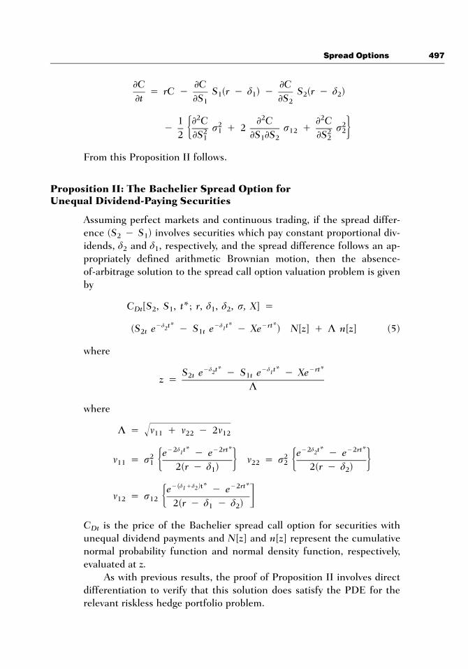
Proposition II: The Bachelier Spread Option forUnequal Dividend-Paying Securities

Assuming perfect markets and continuous trading, if the spread differ-ence (S2 1 S1) involves securities which pay constant proportional div-idends, d2 and d1, respectively, and the spread difference follows an ap-propriately defined arithmetic Brownian motion, then the absence-of-arbitrage solution to the spread call option valuation problem is givenby

C [S , S , t*; r, d , d , r, X] 4Dt 2 1 1 2

1d 1d 1t* t* rt*2 1(S e 1 S e 1 Xe ) N[z] ` K n[z] (5)2t 1t

where

1d 1d 1t* t* rt*2 1S e 1 S e 1 Xe2t 1tz 4K

where

K 4 m ` m 1 2m! 11 22 12

1 d 1 1 d 12 t* 2rt* 2 t* 2rt*1 2e 1 e e 1 e2 2m 4 r m 4 r11 1 22 25 6 5 62(r 1 d ) 2(r 1 d )1 2

1 d `d 1( )t* 2rt*1 2e 1 em 4 r12 12 5 42(r 1 d 1 d )1 2

CDt is the price of the Bachelier spread call option for securities withunequal dividend payments and N[z] and n[z] represent the cumulativenormal probability function and normal density function, respectively,evaluated at z.

As with previous results, the proof of Proposition II involves directdifferentiation to verify that this solution does satisfy the PDE for therelevant riskless hedge portfolio problem.

498 Poitras

The dynamic hedging problem for spread options on futures con-tracts results in a PDE where the restriction that r 1 d 4 0 in eqs. (2)and (3) is imposed due to the ability to create a futures position with nonet investment of funds. For eq. (2), it follows that

2]C 1 ] C24 rC 1 rF 2]t 2 ](F 1 F )1 2

where F2 and F1 are the prices for the relevant futures contract. A similarPDE is related to eq. (3). Given this, the appropriate solution is as follows.

Proposition III: The Bachelier Futures SpreadOption

Assuming perfect markets and continuous trading, for a futures pricespread following arithmetic Brownian motion, the absence-of-arbitragesolution to the spread call option problem is the Bachelier spread optionpricing result:

C [F 1 F , t*; r, r, X] 4Ft 2 1

1rt*e {(F 1 F 1 X) N[u] ` r t* n[u]} (6)!2t 1t F

where

F 1 F 1 X2t 1t 2 2u 4 r 4 r 1 2 r ` rF F F ,F F1 1 2 2r t*!F

CFt is the price of the Bachelier futures spread call option, and N[u] andn[u] represent the cumulative normal probability function and normaldensity function, respectively, evaluated at u.

At present, futures spread options are specified using available con-tract units to determine the value of the commodities being exchanged.For example, one of the New York Mercantile Exchange (NYMEX) crackspread contracts offers an option to exchange futures contracts for crudeoil and heating oil. The LME copper calendar spread option has a similarconfiguration. However, judicious choice of the “prices” used in thespread permits the payoff function to be more appropriately structuredto facilitate speculative trading.

An important illustration of the benefits associated with appropriateselection of units occurs when F1 and F1 refer to contracts for the same

Spread Options 499

commodity but for different delivery dates, a calendar spread option. Forthis example, take F2 and F1 to be the total value of gold represented by,say, the JUNE99 and JUNE98 100 oz. gold contracts, respectively. Eventhough the quantity of gold for each contract is the same, because of thegold futures price contango, F2 and F1 will have different dollar values.For spreads using equal quantities, the change in the spread over timewill be a function of the change in the net implied carry and the changein futures price levels, e.g., Poitras (1990).10 However, when the spreadoption is initially written, F2 and F1 could be equated by tailing thespread. For the gold spread example, this involves taking (F2t/F1t)*100oz. of JUNE98 gold for each 100 oz. of JUNE99 gold. This will equatethe dollar value of the two legs of the spread. This has at least two im-portant implications. First, it simplifies the payoff on the spread optionby making changes in the spread dependent solely on changes in the netimplied carry. Because payoffs depending on changes in price levels areavailable with other options, this would facilitate the market completionproperties of the spread option, supporting demand for the contract. Sec-ond, it means an at-the-money option with an exercise value equal to zerowould have a simple pricing solution, again supporting trade in theoption.

Finally, consistent with an observation made earlier, it is possible toredefine the prices used to specify the spread and model the problem asan arithmetic Brownian motion on one state variable. This is the funda-mental theoretical advantage that assuming the price processes followarithmetic Brownian motions has for solving the spread option pricingproblem. Observing that the sum or difference of normally distributedvariables is also normal permits the spread term in the risk-neutral valu-ation problem to be redefined as a single random variable, y 4 S2T 1

S1T. The resulting changes this redefinition would produce in Proposi-tions I and III are apparent. For these two propositions, modeling thespread using two distinct price processes serves primarily to clarify theprecise form of the volatility process. However, the redefinition requiredto modify Proposition II is much less obvious. While it is still possible tomake a redefinition of the price processes for Proposition II that is con-sistent with modeling the spread as a single random variable, the resultingpricing formula substantively obscures the form of the volatility process.On balance, for practical and pedagogic reasons, Propositions I–III arestated by using distinct price processes.

10Net implied carry is defined as interest and other carry charges net of pecuniary carry returns andconvenience yield.

500 Poitras

OTHER TYPES OF SPREAD AND EXCHANGEOPTIONS

Black-Scholes Exchange Options

To compare the properties of the Bachelier spread options to the lognor-mal case, the spread options are converted to exchange options. An im-portant advantage of spread option solutions based on arithmetic Brown-ian motion is that converting to an exchange option only involves settingX 4 0 in eqs. (4)–(6). The advantage of examining exchange options forgeometric Brownian motion is that, while X ? 0 requires a numericalsolution to a double integral when S2 and S1 or F2 and F1 are jointlylognormal, the X 4 0 lognormal case has a closed form solution. TheBlack-Scholes futures exchange option price differs somewhat from theMargrabe (1978) result, due to the inability to generate cash flows fromthe futures contracts when constructing the riskless hedge portfolio. Asa consequence, the Black-Scholes futures exchange option still retainsthe property of linear homogeneity, but a net investment of funds is re-quired to establish the hedge portfolio leading to the PDE11:

2 2 2]C 1 ] C ] C ] C2 2 2 24 rC 1 r F ` r F ` 2 r F F1 1 2 2 12 1 22 25 6]t 2 ]F ]F ]F ]F1 2 1 2

This leads to the following.

Proposition IV: The Black-Scholes FuturesExchange Option

Assuming perfect markets and continuous trading, if the two prices inthe spread difference (F2 1 F1) involve futures prices which follow con-stant parameter geometric Brownian motions, then the solution to thefutures exchange option valuation problem is given by:

1rt*C 4 e {F N[ f ] 1 F N[ f ]}Bt 2t 1 1t 2

2ln[F /F ] ` (r /2) t*2 1 ff 4 f 4 f 1 r t*!1 2 1 fr t*!f

2 2 2r 4 r 1 2q r r ` r (7)f 1 12 1 2 2

11In specifying the Black-Scholes exchange options the volatility parameters, , are for lognormal2ri

diffusions and are not the same as those used in the section “Bachelier spread option pricing,” whichapply to arithmetic Brownian motion. While the same notation is being used for different parameters,the difference will be apparent from the context.

Spread Options 501

CBt is the price of the Black-Scholes futures exchange option and N[fi]represents the cumulative normal probability function evaluated at fi.

This solution can be proved by direct differentiation of the Black-Scholes futures exchange option formula and verifying that the PDE issatisfied.

Where the securities pay unequal proportional dividends and followseparate geometric Brownian motions, a generalization of Margrabe(1978) provides the following perfect markets, continuous trading resultfor a European exchange option.

Proposition V: The Lognormal Exchange Optionwith Unequal Dividend-Paying Assets

Assuming perfect markets and continuous trading, if the two prices inthe spread difference (S2 1 S1) involve securities which pay constantproportional dividends, d2 and d1, respectively, and the prices follow con-stant parameter geometric Brownian motions, then the solution to theexchange option valuation problem is given by

1d 1dt* t*2 1C 4 S e N[d ] 1 S e N[d ]Ut 2 1 1 2

2ln[S /S ] ` (d 1 d ` r /2) t*2 1 1 2 ud 4 d 4 d 1 r t*!1 2 1 ur t*!u

2 2 2r 4 r 1 2q r r ` r (8)u 1 12 1 2 2

CUt is the price of the Black-Scholes exchange option for securities withunequal dividend payments and N[di] represents the cumulative normalprobability function evaluated at di.

As with the Black-Scholes futures exchange option, Proposition V isproved by direct differentiation of eq. (8) and verifying that the PDE issatisfied. As with Proposition II, Proposition V has considerable practicalvalue for pricing cross-currency exchange swaptions and can be adaptedto pricing cross-currency warrants (e.g., see Dravid, Richardson, and Sun,1994).

Deriving the PDE for the riskless hedge portfolio relevant to secu-rities with unequal dividend payments depends on the linear homogeneityof the Black-Scholes exchange option. This permits the riskless hedgeportfolio to be constructed with no net investment of funds. Recognizingthat the two securities will pay unequal proportional dividends over timeleads to the PDE:

502 Poitras

2 2 2]C 1 ] C ] C ] C2 2 2 24 1 r S ` r S ` 2 r S S1 1 2 2 12 1 22 25 6]t 2 ]S ]S ]S ]S1 2 1 2

]C ]C1 d S 1 d S (9)1 1 2 2]S ]S1 2

The hedge ratios being (exp {1d2} N[d1]) for S2 and 1(exp {1d1} N[d2])for S1, to form the hedge portfolio (S2 exp {1d2} N[d1]) will be sold shortand (N[d2]exp{1d1} S1) purchased with the balance being just sufficientto purchase the spread call option of Proposition V. The self-financingproperty does not apply to the Bachelier exchange option for securitieswith constant but unequal proportional dividends. The solution providedby Proposition II reveals hedge ratios of (exp {1d2} N[z]) and 1(exp {d1}N[z]) for S2 and S1, respectively. The resulting hedge portfolio for X 4 0cannot be constructed without a net investment. Hence, it is not possiblefor r 4 0 requiring rC to appear in the relevant PDE for the risklesshedge portfolio.

The Wilcox Spread Option

The Wilcox spread option is important because it has been acknowledged(e.g., Pearson, 1995; Shimko, 1994) as the spread option pricing formulafor the case where prices follow arithmetic Brownian motion. However,while the formula does have a theoretical foundation in that the solutioncan be motivated by using the risk-neutral valuation problem for a Eu-ropean call option on a nondividend-paying stock, it is possible to dem-onstrate that, as conventionally stated, the Wilcox formula is not consis-tent with absence-of-arbitrage. More precisely, for the single state variablecase12:

1rt*C 4 e E{max [0, S 1 X]}t T

1rt*4 e {E[S 1 X|S $ X] ` E[0|S , X]}T T T

1rt*4 e {E[S 1 X|S $ X]}T T

1rt*4 e {E[S |S $ X] 1 X Prob[S $ X]} (10)T T T

12To be implemented, risk-neutral valuation requires a transition probability density to be specifiedfor evaluating the expectation. Assuming risk neutrality imposes certain conditions on the admissibleform of the transition probability density, typically the restrictions required to apply Girsanov’s the-orem. Risk neutrality also permits discounting by the riskless rate (e.g., see Cox and Ross, 1976, p.153). Stoll and Whalley (1993, chap. 11) provide a useful introduction to risk-neutral valuation witheq. (10) being given on p. 214.

Spread Options 503

where t* 4 (T 1 t)/365, E[•] is the time t expectation taken with respectto the risk-neutral density Prob[•] and r is the riskless interest rate. Forarithmetic Brownian motion, extending this result to spread options in-volves substitution of (S2 1 S1)t for St in eq. (10) to get:

1rt*C 4 e {E[(S 1 S )|(S 1 S ) $ X]T 2T 1T 2T 1T

1 X Prob[(S 1 S ) $ X]} (11)2T 1T

where the E[•] and Prob[•] are for the arithmetic Brownian motion spreadprocess:

d(S 1 S ) 4 a dt ` r dW (12)2 1 s s

where the drift is specified only as some arbitrary constant, as, which mayor may not be some function of S2, S1, and t.

Evaluation of the expectation in eq. (11) using the probability densityassociated with eq. (12) leads to the following.

Proposition VI: The Wilcox Spread OptionFormula

Assuming perfect markets and continuous trading, for a price spread fol-lowing eq. (12), the solution to the valuation problem (11) provides theWilcox spread option pricing result:

C (S 1 S , t*; r, r, X) 4W 2 1

1rt*e {((S 1 S ) ` a t* 1 X) N[w] ` r t* n[w]} (13)!2t 1t S S

where

(S 1 S ) ` a t* 1 X2t 1t Sw 4r t*!S

and N[w] and n[w] represent the cumulative normal probability functionand normal density function, respectively, evaluated at w.

Evaluating the appropriate derivatives of this solution and comparingwith the PDE (3) where d 4 0 reveals that the Wilcox formula does notconform to absence-of-arbitrage due to the presence of the arbitrary pa-rameter alpha. This inconsistency raised by the presence of as in Propo-sition VI is intuitive because as does not appear in either the PDE (3) orthe associated boundary condition, indicating that the absence-of-arbi-trage solution will be independent of as.

504 Poitras

It is possible to develop the Wilcox solution further to identify therestrictions which are imposed on eq. (12) for absence-of-arbitrage. Tobe consistent with absence-of-arbitrage, it is necessary for eq. (13) tosatisfy eq. (2). This leads to the following.

Corollary VI.1: The Absence-of-ArbitrageCoefficient Restrictions on the Bachelier Option

For the solution (13) to satisfy the PDE (2), the drift coefficient in eq.(12) must satisfy the restriction as 4 r(S2 1 S1).

More precisely, Corollary VI.1 indicates that eq. (12) has to be inthe form of an OU process to satisfy absence-of-arbitrage. The require-ment of a nonconstant drift also impacts the volatility used in PropositionVI, which must be rescaled and will be nonconstant. The absence-of-arbitrage restriction is reflected in Propositions I–III. In other words,using the risk-neutral valuation approach associated with eq. (11) wouldhave provided the correct solution if the probability space had been cor-rectly defined.

Spread Option Prices for Absorbed BrownianMotion

If unrestricted arithmetic Brownian motion has the appealing feature ofproviding simpler and more readily implementable closed form solutionsfor option prices, how do these closed forms compare to solutions ob-tained using absorbed Brownian motion? Addressing this question re-quires some consideration of the transition probability density for thespread option, under both absorbed and unrestricted Brownian motion.The importance of the transition density can be identified by consideringthe risk-neutral valuation procedure. On the expiration date, the payouton a spread option has the form, CT 4 max[S2T 1 S1T 1 X, 0]. Risk-neutral valuation determines the spread option pricing formula by eval-uating the discounted expected value of the expiration date payout, wherethe expected value calculation is taken over the assumed probability spacefor the S2 and S1 state variables, a bivariate normal transition probabilitydensity. Evaluating this expected value is decidedly less complicated forunrestricted than for absorbed Brownian motion (Heaney and Poitras,1997).

The transition probability density for a spread option calculated us-ing two price processes which both follow absorbed Brownian motion canbe motivated by generalizing the single variable case given in Cox and

Spread Options 505

Ross (1976, p. 162), in Goldenberg (1991, p. 7), and, more rigorously, inKarlin and Taylor (1975, pp. 354–355). In this case, the transition prob-ability density is specified as the difference between the unrestricted den-sity and the density associated with the paths where the state variablegoes negative. By ignoring the economic restriction that state variableprices must be nonnegative, call option valuation assuming unrestrictedBrownian motion provides a higher theoretical price than for absorbedBrownian motion. The unrestricted solution attaches value to those statevariable paths which reach zero and continue on to exceed the exerciseprice at a later time. Under absorbed Brownian motion, these paths willbe absorbed at zero and will be assigned a zero value. It follows that thedifference between the absorbed and unrestricted solutions, if any, willdepend on the density associated with these paths which, in turn, willdepend on the exercise price level and the probability of absorption, afunction of the maturity of the option, the initial price, and the volatilityof the state variable process.

For the spread option, the expectation taken using the joint densityassociated with the absorbed Brownian motions can be modeled using afour-part density. As in the single variable case, one part applies to theunrestricted paths of S1t and S2t. Hence, as in the single variable case,the unrestricted call option price provides an upper bound on the callprice determined using absorbed Brownian motion. The unrestricted den-sity is adjusted by differencing out the second and third parts of thedensity which apply to paths where one of S1t or S2t is absorbed at zeroand the other path is unrestricted. The fourth part of the density accountsfor the bias in the second and third parts of the density introduced byignoring cases where both S1t and S2t are absorbed. This density is con-ditional, depending on the probability that one price reaches zero giventhat the other variable also reaches zero. While useful for illustrating therelationship between the univariate and spread option solutions, thisfour-part decomposition of the joint density required for risk-neutral valu-ation of the spread option is not the only method for determining theprice formula (Heaney and Poitras, 1997).

In general, when the risk-neutral expectation of the spread option isevaluated, each of the four parts of the decomposed joint density willproduce corresponding terms in the closed form option price. Even inthe case of independent random variables, specification of the relevantdensities and evaluation of the risk-neutral integrations are complex. Al-lowing the random variables to be dependent makes the problem evenmore difficult. The resulting closed form solution will be complicated,whatever the approach used to model the joint density. Taking the expec-

506 Poitras

tation for unrestricted Brownian motion does not require decompositionof the joint density, substantively reducing the number of terms in theclosed form option price. This gain in analytical simplicity is desirable ifthe intuitive disadvantages of assuming unrestricted Brownian motion donot have a significant impact on the pricing of spread options. In partic-ular, if it is not possible for the prices composing the spread (S2 1 S1)to have negative values before the maturity date of the option, the solu-tions for the unrestricted and absorbed cases will be identical for practicalpurposes. In terms of the four-part decomposition of the joint density,those parts associated with one or both of the prices being absorbed willbe zero and the call option solution will be reduced to the unrestrictedcase.

SIMULATION OF SPREAD AND EXCHANGEOPTION PRICES

The closed form spread option prices provided in the section “BachelierSpread Option Pricing” have the desirable characteristic of simplicity. Isthis simplicity achieved at the expense of pricing accuracy? Because aspread option is being priced, answering this question is more compli-cated than for options involving one security price. In particular, the cor-relation between the prices in the spread introduces an additional di-mension to the comparisons. When evaluating option prices associatedwith Propositions I and II, another complication also arises in determin-ing the volatility for the arithmetic process. In order to initially avoid thiscomplication, Table I provides a summary of simulated futures spreadcall prices for Proposition III with selected values of F1, t*, and q12, thecorrelation between F1 and F2. Considerable variation in pricing is ob-served as the absolute value of q increases. One practical implication ofthis result is that calendar spread options typically will have q12 in the0.9 region and many intercommodity spread options often will have q12

in the 0–0.5 region. Hence, even though the same initial dollar valuesmay be traded, the prices for different types of spread options will haveconsiderable variation, depending on the correlation in the state variableprices.

The parameters in Table I are selected to provide rough compara-bility with Pearson (1995, exhibit 5): F2 is fixed at 100 with X 4 4 and r4 0.1. Unfortunately, direct comparison is not possible because Pearson(1995) evaluates a Wilcox option solution similar to eq. (13) and, in theprocess, uses an inappropriate method of determining the volatility. Moreprecisely, to simulate the Wilcox prices, Pearson (1995) estimates as em-

Spread Options 507

TABLE I

Bachelier Futures Spread Call Option Prices for Different Parameter Values

Price of F1/Correlation

q12 F1

Time to Maturity (in Years)

0.08 2 3 4 5

0 95 3.808 11.389 14.140 15.489 16.07997 2.816 10.491 13.328 14.754 15.41499 2.013 9.6411 12.547 14.042 14.767

101 1.386 8.8370 11.796 13.352 14.138103 0.919 8.0792 11.075 12.685 13.526105 0.585 7.3670 10.384 12.041 12.933

0.5 95 2.855 8.1892 10.120 11.062 11.46997 1.863 7.2915 9.308 10.327 10.80499 1.134 6.4601 8.539 9.624 10.164

101 0.640 5.6944 7.813 8.953 9.549103 0.333 4.9932 7.130 8.314 8.960105 0.158 4.3549 6.489 7.707 8.396

0.9 95 1.610 3.9252 4.760 5.157 5.31897 0.618 3.0276 3.948 4.422 4.65399 0.164 2.2770 3.232 3.759 4.045

101 0.028 1.6673 2.610 3.166 3.492103 0.003 1.1870 2.078 2.642 2.993105 0.0002 0.8205 1.631 2.184 2.548

10.5 95 4.544 13.847 17.228 18.889 19.62097 3.552 12.950 16.416 18.154 18.95599 2.714 12.090 15.629 17.437 18.305

101 2.025 11.269 14.866 16.740 17.669103 1.473 10.486 14.129 16.060 17.048105 1.044 9.740 13.416 15.399 16.441

10.9 95 5.045 15.519 19.328 21.200 22.02897 4.053 14.621 18.515 20.465 21.36399 3.198 13.758 17.725 19.747 20.711

101 2.477 12.928 16.958 19.045 20.072103 1.881 12.132 16.212 18.360 19.446105 1.399 11.370 15.488 17.691 18.833

Notes: The following fixed values are used to calculate the spread option prices: F2 4 100, r 4 0.1, X 4 4, r1 4 r2 4

20.78.

pirically and, to determine rs, assumes both S2 and S1 are lognormal.More precisely, Pearson (1995) assumes:

2 2 2 2 2r 4 r S 1 2r S S ` r S a 4 (r 1 d )S 1 (r 1 d )SS 1 1 12 1 2 2 2 S 2 2 1 1

However, this method of specifying the volatility is inconsistent with theassumption of constant parameters used to specify eq. (12) and, as aresult, the simulated Wilcox prices will not satisfy the relevant PDE forthe dynamic hedging problem if these parameter values are used. Pearson

508 Poitras

(1995) compares the resulting Wilcox option price estimates with pricesdetermined from a double-integral lognormal solution which is evaluatednumerically. Pearson (1995) reports substantial deviations between theWilcox option prices and the more complex double-integral solution whent* is large.

Using the same F2, T, and r12 values as in Table I, the Black-Scholesand Bachelier futures exchange option prices are calculated and reportedin Table II. By retaining the same parameters as for Table I, the impactof changing from X 4 4 to X 4 0 can be determined by examining theBachelier prices. As expected, the impact is largest for short maturity, in-the-money options, e.g., an increase of $3.38 for t* 4 0.08, S1 4 95,and q12 4 0.9. Much smaller differences are observed for the longestmaturity options, e.g., an increase of $1.50 for t* 4 5, S1 4 95, and q12

4 0.9. At any given maturity, the difference increases with q12. Examiningthe differences between the Black-Scholes and Bachelier exchange optionprices reported in Table II, the general similarity of the prices is striking.The primary source of difference is that Black-Scholes prices are lessaffected as q12 increases. The absolute size of the difference between theBlack-Scholes and Bachelier prices increases with maturity. At any givent* and q12, price differences are larger for out-of-the-money than in-the-money spread options.

The results in Table II are significantly different than those providedin Pearson (1995, exhibits 2 and 5), where much wider differences be-tween Black-Scholes and Bachelier spread option prices were observed.There are a number of possible reasons for the discrepancy. Futures vol-atility misspecification is one potential reason for this discrepancy, thoughresults in Table I indicate that this is not likely to be a substantive sourceof pricing error. The use of exchange options instead of spread options isalso not likely to be a source of differences in the Bachelier and Black-Scholes prices, e.g., due to the linear impact of X on the Bachelier prices.Another possible difference is that Pearson (1995) uses the Wilcox so-lution, which differs from eq. (6) in a number of ways, such as the needto provide an estimate for the drift of the spread process. Finally, a fun-damental parametric difference is that Table II is calculated for futuresprices, while Pearson (1995) evaluates a physical security which incor-porates dividends. Comparison of eq. (6) with eqs. (4) and (5) reveals anumber of important differences. Significantly, eqs. (4) and (5) involvesecurity volatility estimates which depend on t*, r, and d in a complicatedfashion.

Table III reveals that the impact of introducing dividend paymentson the difference between Bachelier and Black-Scholes exchange option

Spread Options 509

TABLE II

Bachelier and Black-Scholes Futures Exchange Call Option Prices for DifferentParameter Values

Price of F1/Correlation

q12 F1

Time to Maturity (in Years)

0.08 2 3 4 5

Bachelier Options0 95 6.347 13.325 15.857 17.027 17.463

97 4.989 12.334 14.983 16.246 16.76299 3.808 11.389 14.140 15.489 16.079

101 2.816 10.491 13.328 14.754 15.414103 2.013 9.641 12.547 14.042 14.767105 1.386 8.837 11.796 13.352 14.138

0.5 95 5.602 10.192 11.887 12.642 12.88997 4.113 9.163 10.988 11.842 12.17399 2.858 8.199 10.133 11.075 11.483

101 1.866 7.301 9.321 10.341 10.818103 1.136 6.470 8.552 9.638 10.178105 0.642 5.704 7.826 8.967 9.564

0.9 95 4.988 6.155 6.671 6.841 6.91797 3.140 4.969 5.668 5.964 6.03999 1.610 3.925 4.760 5.157 5.318

101 0.618 3.027 3.948 4.422 4.653103 0.164 2.277 3.232 3.759 4.045105 0.028 1.667 2.610 3.166 3.492

Black-Scholes Options0 95 6.179 12.624 14.928 15.955 16.298

97 4.828 11.732 14.183 15.317 15.74699 3.670 10.890 13.470 14.703 15.212

101 2.709 10.097 12.789 14.112 14.697103 1.941 9.352 12.139 13.544 14.199105 1.349 8.653 11.518 12.998 13.718

0.5 95 5.680 10.534 12.301 13.077 13.31997 4.233 9.594 11.511 12.396 12.72699 3.017 8.717 10.763 11.746 12.156

101 2.050 7.903 10.055 11.125 11.610103 1.324 7.148 9.386 10.533 11.087105 0.812 6.452 8.754 9.969 10.585

0.9 95 5.065 7.067 7.871 8.182 8.22297 3.335 5.989 6.968 7.400 7.53699 1.925 5.024 6.140 6.673 6.894

101 0.946 4.173 5.385 6.002 6.295103 0.387 3.430 4.702 5.383 5.737105 0.130 2.791 4.087 4.815 5.220

Notes: The exchange call option prices are for futures contracts. The following fixed values are used to calculate theBachelier exchange option prices: F2 4 100, r 4 0.1, X 4 0, r1 4 r2 4 20.78. The following fixed values are used tocalculate the Black-Scholes exchange option prices: F2 4 100, r 4 0.1, X 4 0, r1 4 r2 4 0.2.

510 Poitras

TABLE III

Bachelier and Black-Scholes Exchange Call Option Prices for DifferentParameter Values and Dividend-Paying Securities

Price of S1/Correlation

q12 S1

Time to Maturity (in Years)

0.08 2 3 4 5

Bachelier Options0 95 5.999 12.277 14.951 16.496 17.414

97 4.582 11.206 13.956 15.558 16.52499 3.366 10.194 13.003 14.654 15.663

101 2.370 9.241 12.093 13.783 14.830103 1.592 8.348 11.224 12.946 14.027105 1.017 7.514 10.398 12.144 13.253

0.5 95 5.411 9.514 11.339 12.386 12.99697 3.848 8.395 10.310 11.420 12.08299 2.547 7.359 9.340 10.501 11.209

101 1.551 6.406 8.429 9.631 10.377103 0.859 5.537 7.578 8.808 9.586105 0.429 4.752 6.786 8.033 8.835

0.9 95 4.993 6.042 6.680 7.036 7.22197 3.088 4.732 5.512 5.956 6.20999 1.489 3.595 4.470 4.980 5.287

101 0.493 2.642 3.559 4.109 4.454103 0.099 1.874 2.780 3.344 3.712105 0.011 1.279 2.127 2.683 3.059

Black-Scholes Options0 95 6.206 13.396 16.737 18.901 20.398

97 4.850 12.450 15.902 18.145 19.70799 3.686 11.557 15.103 17.417 19.039

101 2.721 10.715 14.340 16.718 18.394103 1.949 9.924 13.610 16.044 17.771105 1.355 9.182 12.915 15.397 17.169

0.5 95 5.526 10.300 12.617 14.126 15.17397 4.022 9.277 11.709 13.296 14.40799 2.770 8.330 10.852 12.507 13.676

101 1.796 7.456 10.045 11.758 12.977103 1.092 6.654 9.288 11.047 12.309105 0.620 5.920 8.578 10.373 11.673

0.9 95 5.001 6.334 7.198 7.766 8.15497 3.127 5.091 6.106 6.770 7.23299 1.576 4.010 5.129 5.865 6.385

101 0.589 3.092 4.265 5.049 5.613103 0.153 2.334 3.511 4.319 4.912105 0.026 1.724 2.862 3.672 4.281

Notes: The following fixed values are used to calculate the Bachelier exchange option prices: S2 4 100, r 4 0.1, X 4 0,uv11 4 uv12 4 16.30, d1 4 d2 4 0.045. The following fixed values are used to calculate the Black-Scholes exchange optionprices: S2 4 100, r 4 0.1, X 4 0, r1 4 r2 4 0.2, d1 4 d2 4 0.045.

Spread Options 511

prices is substantial. Determining volatility (K) is a major difficulty incalculating the Bachelier exchange options in Table III. One source ofdifficulty is the singularity point in v12 of Proposition II which preventsthe use of the d1 and d2 used by Pearson. There are similar singularitypoints in v11 and v22. No attempt is made to determine a specific volatilityto calibrate the exchange option prices, though there appears to be cali-bration at q12 4 0.9, t* 4 0.08, and S1 4 95. The v11 and v22 valuesused are determined by solving the implied V for an individual securityusing the same call price as for a constant proportional dividend Black-Scholes call calculated using the parameter values associated with TableIII, e.g., r 4 0.2. To determine the appropriate K for q12 4 0.5 and 0.9,the relevant value for v12 is directly calculated. Bachelier prices are rela-tively unchanged from Table II, while Black-Scholes prices exhibit muchlarger changes, particularly with small q12 and large t*.

The advantage of selecting the specific r, d, and r values used inTable III is that a rough comparison with Pearson is permitted. In as-sessing the differences in the Black-Scholes and Bachelier prices, impli-cations of the method used to determine Bachelier volatility (K) and theimplied calibration of prices have to be recognized. Calibrating prices fora specific volatility would involve selecting some initial parameter valuesand determining the volatilities required for the Black-Scholes and Bach-elier prices to be equal.13 Given this, Table III generally confirms thedifferences reported by Pearson (1995). Substantial pricing differencesare observed, particularly for the long maturity, low q12 cases. This dif-ference would be even larger if negative q12 results were reported. Com-parison of the Black-Scholes results of Table III with Pearson (1995,exhibit 2) can also provide an assessment for the impact of exercise pricechanges on the Black-Scholes spread option. Results similar to those fromthe comparison of Bachelier prices in Tables I and II are observed. Thisindicates a possibility for developing easily calculated heuristic prices forBlack-Scholes spread options by using the Black-Scholes exchange optionsolution, with an adjustment for the exercise price effect.

CONCLUSIONS

Spread trading is an important source of liquidity in both cash and futuresmarkets. Wide variation in the types of spreads being traded can be iden-tified. Just in the futures market there are credit spreads, such as theTED spread between Eurodollar and Treasury bill rates; production

13Some method of calibration is required because Black-Scholes volatility is for returns, while Bach-elier volatility is for prices.

512 Poitras

spreads, such as the soybean crush spread between prices for soybeans,soybean meal, and soybean oil or the crack spread between prices forcrude oil, heating oil, and gasoline; tailed or untailed calendar spreadsbetween the prices for the same commodity on different delivery dates(e.g., see Yano, 1989) and maturity spreads, such as the NOB spreadbetween prices for Treasury notes and Treasury bonds. In addition tothese trades, the cash market also features spreads for other commoditiesas well as spreads based on variations in grade and location. Despite theconsiderable potential for spread option trading to support cash and fu-tures market activity, there is only relatively restricted trading in optionson price differences. There are only a few exchange traded contracts andactivity in the OTC market is limited.

Spread option pricing is complicated by the presence of two randomvariables. Because the spread distribution will be the convolution of twodistributions, closed form solutions for spread options are difficult to de-termine in general. For the conventional options pricing assumption oflognormally distributed random variables and nonzero exercise price,closed form solutions are not available and numerical methods are re-quired to determine option prices. This article exploits the linearity prop-erties of arithmetic Brownian motion to specify closed forms for threetypes of spread option prices: securities paying equal and unequal divi-dends and futures prices. The solutions provided are referred to as Bach-elier spread options. To provide a pricing comparison with solutions as-suming lognormally distributed prices, relevant exchange option pricesfor the lognormal case are derived. Bachelier and Black-Scholes exchangeoption prices are then compared and differences identified. For spreadsinvolving the difference of two futures prices, the Black-Scholes andBachelier spread option prices are similar. However, sizable pricing dif-ferences are observed for spread options involving securities making div-idend payments. These differences are partly due to difficulties in deter-mining volatility for the arithmetic processes and, in turn, calibrating thatvolatility to the lognormal case.

APPENDIX

Proof of Proposition I

The derivations in the following propositions require the result that

2]n[g] ] 1 ]{1g /2} ]g ]g21g /24 e 4 n[g] 4 n[g] (1g)]x ]x ]g ]x ]x2p!

Spread Options 513

Given this, the proof proceeds by treating the spread as a single randomand evaluating the PDE (2). For ease of notation, let (S2 1 S1) 4 S andobserve that the relevant derivatives of eq. (4) are now

]C ]N ]n1d 1d 1 1dt* t* rt* t*4 e N[h] ` (Se 1 Xe ) ` V 4 e N[h]]S ]S ]S

1 d2 2 t*] C ]N ]h e1d 1dt* t*4 e 4 e n[h] 4 n[h]2]S ]S ]S V

]C ]N1d 1 1d 1t* rt* t* rt*4 (1dSe ` rXe ) N[h] ` (Se 1 Xe )]t* ]t*

]V ]n` n[h] ` V

]t* ]t*

]C ]V1d 1t* rt*4 1 4 (1dSe ` rXe ) N[h] ` n[h]]t ]t*

Substitution back into the PDE and canceling leads to

t*1d]V 1 e21 n[h] 4 r V n[h] 1 r n[h]]t* 2 V

1/21 d 1 1 d 1 1d2 2 t* 2rt* 2 2 t* 2rt* t*r 1d e 1 r e r (e 1 e ) 1 e21 4 r 1 r5 6 1 22V r 1 d 2(r 1 d) 2 V

Multiplying through by V and then by [2(r 1 d)]/r2 and canceling provesthe proposition. Derivatives for verifying that eq. (4) also obeys eq. (3)can be obtained by examining and, where appropriate, simplifying thesolutions to Proposition II.

Proof of Proposition II

For ease of notation, let Ci denote partial differentiation with respect toSi. Second derivatives are similarly defined. The relevant derivatives ofeq. (5) are

514 Poitras

1d 1dt* t*1 2C 4 e N[z] C 4 1e N[z]1 2

1d 1d 1 d `dt* t* ( )t*1 21 2e e eC 4 n[z] C 4 n[z] C 4 1 n[z]11 22 12V V V

]C ]C 1d 1d 1t* t* rt*2 14 1 4 (1d S e ` d S e ` rXe ) N[z]2 2 1 1]t* ]t

]N ]V ]n1d 1d 1t* t* rt*2 1` (S e 1 S e 1 Xe ) ` n[z] ` V2 1 ]t* ]t* ]t*

]V1d 1d 1t* t* rt*2 14 (1d S e ` d S e ` rXe ) N[z] ` n[z]2 2 1 2 ]t*

Substituting these results back into the PDE and canceling terms leaves:

]V 1 1 d 1d 1 d `d2 2 t* 2 t* ( )t*1 2 1 2n[z] 4 rVn[z] 1 (r e ` r e 1 2r e ) n[z]1 2 12]t* 2V

Evaluating {]V/]t*}, cross-multiply by 12V and cancel n[z], which iscommon to all terms. All terms involving r e1rt* now cancel. Collectingthe remaining terms from rVn[z] and {]V/]t*} and canceling the denom-inators where appropriate, the remaining terms all cancel, which provesthe proposition.

Proof of Proposition III

The relevant derivatives of eq. (6) are

12 rt*]C ] C e1rt*4 e N[k] 4 n[k]2]F ]F r t*!

]C ]N1 1rt* rt*4 1r e [(F 1 X) N[k] ` r t* n[k]] ` e (F 1 X)!]t* ]t*

r ]n ]C1 1rt* rt*` e n[k] ` e r t* 4 1!]t* ]t2 t*!

r1 1rt* rt*4 1r e [(F 1 X) N[k] ` r t* n[k]] ` e n[k]!2 t*!

Substitution back into the PDE and canceling proves the proposition.

Spread Options 515

Proof of Proposition VI

From eq. (12), over the time interval starting at t and ending at T, witht* 4 (T 1 t)/365:

S 1 S 1 at*T tS 4 S ` at* ` r t* Z or Z 4!T tr t*!

where Z is N(0,1). Evaluating eq. (10) gives:

S ` at* 1 XtX Prob[S $ X] 4 X NT 3 4r t*!

``

E[S |S $ X] 4 (S ` at* ` r t* Z) n[Z] dZ!T T t#(X1S 1at*)/r t*!t

` 1 r(S at* X)/ t*! ``t

4 (S ` at*) n[Z] dZ ` r t* Z n[Z] dZ!t # #1` (X1S 1at*)/r t*!t

S ` at* 1 X S ` at* 1 Xt t4 (S ` at*) N ` r t* n!t 3 4 3 4

r t* r t*! !

Substituting these results into eq. (10) and observing the definition of ggives Proposition VI.

Proof of Corollary VI.1

Given the rule for differentiating n[•], the relevant derivatives of eq. (13)are

]C ]N ]n1 1rt* rt*4 e N[g] ` (S ` at* 1 X) ` r t* 4 e N[g]!5 6]S ]S ]S

2] C ]N ]g n[g]1 1 1rt* rt* rt*4 e 4 e n[g] 4 e2]S ]S ]S r t*!

]C ]C4 1 4 1rC `

]t* ]t

]N 1 r ]n1rt*e aN ` (S ` at* 1 X) ` n[g] ` r t*!5 6]t* 2 ]t*t*!

1 r1rt*4 1rC ` e aN ` n[g]5 62 t*!

Substituting these results into eq. (2) and canceling proves the corollary.

516 Poitras

BIBLIOGRAPHY

Austin, M. (1990): “A Modification and Re-examination of the Bachelier OptionPricing Model,” American Economist, (Fall): 34–41.

Bachelier, L. (1900): “Theory of Speculation” (English translation) in Cootner,The Random Character of Stock Market Prices, 17–78.

Ball, C., and Roma, A. (1994): “Stochastic Volatility Option Pricing,” Journal ofFinancial and Quantitative Analysis, 29:589–607.

Bjerksund, P., and Stensland, G. (1994): “An American Call on the Differenceof Two Assets,” International Review of Economics and Finance, 3:1–26.

Black, F., and Scholes M. (1973): “The Pricing of Options and Corporate Lia-bilities,” Journal of Political Economy, 81:637–654.

Brennan, M. (1979): “The Pricing of Contingent Claims in Discrete Time Mod-els,” Journal of Finance, 24:53–68.

Brooks, R. (1995): “A Lattice Approach to Interest Rate Option Spreads,” Journalof Financial Engineering, 4:281–296.

Carr, P. (1988): “The Valuation of Sequential Exchange Opportunities,” Journalof Finance, 43:1235–1256.

Cootner, P. (1964): The Random Character of Stock Market Prices. Cambridge,MA: MIT Press.

Cox, D., and Miller, H. (1965): The Theory of Stochastic Processes. London:Chapman & Hall.

Cox, J., and Ross, S. (1976): “The Valuation of Options for Alternative StochasticProcesses,” Journal of Financial Economics, 3:145–166.

Dravid, A., Richardson, M., and Sun, T. (1994): “The Pricing of Dollar-Denom-inated Yen/DM Warrants,” Journal of International Money and Finance,13:517–536.

Falloon, W. (1992): “Promise and Performance,” Risk, 5(9):31–32.Fu, Q. (1996): “On the Valuation of an Option to Exchange One Interest Rate

for Another,” Journal of Banking and Finance, 20:645–653.Gibson, R., and Schwartz, E. (1990): “Stochastic Convenience Yield and the

Pricing of Oil Contingent Claims,” Journal of Finance, 45:959–976.Goldenberg, D. (1991): “A Unified Method for Pricing Options on Diffusion

Processes,” Journal of Financial Economics, 29:3–34.Grabbe, O. (1995): “Copper-Bottom Pricing,” Risk, May:63–66.Heaney, J., and Poitras, G. (1997): “Unrestricted versus Absorbed Arithmetic

Brownian Motion for Pricing Different Types of Options.” Working paper,Simon Fraser University, Burnaby, British Columbia, Canada.

Jarrow, R., and Rudd, A. (1982): “Approximate Option Valuation for ArbitraryStochastic Processes,” Journal of Financial Economics, 10:347–369.

Karlin, S., and Taylor, H. (1975): A First Course in Stochastic Processes. 2nd ed.New York: Academic Press.

Margrabe, W. (1978): “The Value of an Option to Exchange One Asset for An-other,” Journal of Finance, 33:177–186.

Merton, R. (1973): “The Theory of Rational Option Pricing,” Bell Journal ofEconomics and Management Science, 4:141–183.

Pearson, N. (1995): “An Efficient Approach for Pricing Spread Options,” Journalof Derivatives, Fall:76–91.

Spread Options 517

Poitras, G. (1990): “The Distribution of Gold Futures Spreads,” The Journal ofFutures Markets, 10:643–659.

Ravindran, K. (1993): “Low-Fat Spreads,” Risk, October:66–67.Rechner, D., and Poitras, G. (1993): “Putting on the Crush: Day Trading the

Soybean Complex Spread,” The Journal of Futures Markets, 13:61–75.Rubinstein, M. (1991a): “Exotic Options.” Working paper no. 220, University of

California at Berkeley.Rubinstein, M. (1991b): “Somewhere over the Rainbow,” Risk, November:63–

66.Samuelson, P. (1965): “Rational Theory of Option Pricing,” Industrial Manage-

ment Review, 6:13–31.Shimko, D. (1994): “Options on Futures Spreads: Hedging, Speculation and

Valuation,” The Journal of Futures Markets, 14:183–213.Smith, C. (1976): “Option Pricing: A Review,” Journal of Financial Economics,

3:3–51.Stoll, H., and Whalley, R. (1993): Futures and Options. Cincinnati:

Southwestern.Wilcox, D. (1990): Energy Futures and Options: Spread Options in Energy Mar-

kets. New York: Goldman Sachs & Co.Yano, A. (1989): “Configurations for Arbitrage Using Financial Futures,” The

Journal of Futures Markets, 9:439–488.