Embed Size (px)
Citation preview

Spreading and Precoding for WirelessMIMO-OFDM Systems
DISSERTATION
zur Erlangung des akademischen Gradeseines
DOKTOR-INGENIEURS(DR.-ING.)
der Fakultat fur Ingenieurwissenschaftenund Informatik der Universitat Ulm
von
DORIS YASMOU YACOUB
AUS HELIOPOLIS/KAIRO
1. Gutachter: Prof. Dr.–Ing. Jurgen Lindner
2. Gutachter: Prof. Dr. rer. nat. Dr. h. c. Hermann Rohling
Amtierender Dekan: Prof. Dr. rer. nat. Helmuth Partsch
Ulm, 13. Juni 2008

Acknowledgments
First, I would like to express my warm and sincere gratitude to my supervisorProfessor Jurgen Lindner for giving me the opportunity to join his researchgroup at the Institute of Information Technology, Ulm University as wellas for his understanding, personal guidance, and for his important andunfailing support throughout this work.
I also wish to express my sincere thanks to Professor Hermann Rohling, Headof the Telecommunications Institute at Technische Universitat Hamburg-Harburg, not just for being a co-reviewer of this thesis, but also for givingme the opportunity to participate in the OFDM-Workshop for several yearsof which I have very fond memories.
My warm thanks are also due to Dr. Werner G. Teich for his sincere adviceand friendly help. His discussions about my work have always been veryhelpful.
I also wish to give a special thanks my colleague and friend Ivan Perisafor his support throughout those years. My sincere thanks are also due toall my colleagues for many valuable discussions and for proof-reading thisthesis.
Last but not least, my warm and loving thanks to my husband HendrikRoscher for his unceasing support and encouragement throughout.
Doris Y. Yacoub
Ulm, June 2008

Contents
1 Introduction 1
2 Theoretical Background 3
2.1 MIMO Channel Model . . . . . . . . . . . . . . . . . . . . . . . . . 4
2.2 Orthogonal Frequency Division Multiplexing . . . . . . . . . . . . 5
2.2.1 SISO-OFDM . . . . . . . . . . . . . . . . . . . . . . . . . . . 5
2.2.2 MIMO-OFDM . . . . . . . . . . . . . . . . . . . . . . . . . . 11
2.2.3 Spreading . . . . . . . . . . . . . . . . . . . . . . . . . . . . 14
2.3 Correlated MIMO-OFDM Channel Model . . . . . . . . . . . . . . 16
2.4 Effect of Antenna Correlations . . . . . . . . . . . . . . . . . . . . 19
2.4.1 Channel Condition Number . . . . . . . . . . . . . . . . . . 19
2.4.2 Diversity and Correlation Measures . . . . . . . . . . . . . 19
2.5 Block Equalizers . . . . . . . . . . . . . . . . . . . . . . . . . . . . 22
2.5.1 Hard Decision Equalizers . . . . . . . . . . . . . . . . . . . 23
2.5.2 Soft Decision Equalizers . . . . . . . . . . . . . . . . . . . 25
2.6 Iterative Equalization and Decoding . . . . . . . . . . . . . . . . . 29
2.7 Test Channels . . . . . . . . . . . . . . . . . . . . . . . . . . . . . 34
2.8 Summary . . . . . . . . . . . . . . . . . . . . . . . . . . . . . . . . 40
3 Spreading 41
3.1 Diversity . . . . . . . . . . . . . . . . . . . . . . . . . . . . . . . . . 42
3.2 Space Time and Space Frequency Codes . . . . . . . . . . . . . . 44
3.3 Spreading Criteria for MIMO-OFDM . . . . . . . . . . . . . . . . . 46
3.4 MC-Code Division Multiplexing . . . . . . . . . . . . . . . . . . . 48
3.5 MC-Cyclic Antenna Frequency Spreading . . . . . . . . . . . . . 49
3.6 Spreading, Matched Filter Bound and Interference . . . . . . . . 59
3.6.1 Effect of Antenna Correlations on Interference and MFB . 62
3.6.2 Asymptotic Behavior of α and β . . . . . . . . . . . . . . . 66
3.6.3 Effect of Interference Distribution on the BER . . . . . . . 70
I
Contents
3.7 Rotated MC-CAFS . . . . . . . . . . . . . . . . . . . . . . . . . . . 72
3.7.1 Rotations Type I . . . . . . . . . . . . . . . . . . . . . . . . 73
3.7.2 Rotations Type II . . . . . . . . . . . . . . . . . . . . . . . . 73
3.8 Coded Transmission . . . . . . . . . . . . . . . . . . . . . . . . . . 81
3.9 Summary . . . . . . . . . . . . . . . . . . . . . . . . . . . . . . . . 84
3.A Appendix to Chapter 3 . . . . . . . . . . . . . . . . . . . . . . . . . 85
3.A.1 Expected Values of Functions of Correlated Complex Ran-dom Variable for Kronecker Correlation Model . . . . . . . 85
3.A.2 Expected values of α, β and the var(r) . . . . . . . . . . . . 87
4 Precoding 91
4.1 Linear Precoding . . . . . . . . . . . . . . . . . . . . . . . . . . . . 92
4.2 Full Channel Knowledge at the Transmitter . . . . . . . . . . . . 93
4.3 Partial Channel Knowledge at the Transmitter . . . . . . . . . . 94
4.3.1 Flat Fading Channels . . . . . . . . . . . . . . . . . . . . . 95
4.3.2 Frequency Selective Channels . . . . . . . . . . . . . . . . 96
4.4 Uncoded Transmission . . . . . . . . . . . . . . . . . . . . . . . . 99
4.4.1 Imperfect Transmit Correlation Knowledge . . . . . . . . . 102
4.4.2 Different Antenna Correlation at each Channel Tap . . . 105
4.5 Coded Transmission . . . . . . . . . . . . . . . . . . . . . . . . . . 107
4.6 Summary . . . . . . . . . . . . . . . . . . . . . . . . . . . . . . . . 118
4.A Appendix to Chapter 4 . . . . . . . . . . . . . . . . . . . . . . . . . 120
4.A.1 Antenna Correlations in Frequency Domain . . . . . . . . 120
4.A.2 BER curves and EXIT-Charts . . . . . . . . . . . . . . . . 121
5 MIMO Channel Capacity: Theory versus Measurement 131
5.1 MIMO Channel Capacity . . . . . . . . . . . . . . . . . . . . . . . 131
5.1.1 No channel knowledge at the transmitter . . . . . . . . . . 132
5.1.2 Full channel knowledge at the transmitter . . . . . . . . . 134
5.1.3 Partial channel knowledge at the transmitter . . . . . . . 135
5.1.4 Impact of Antenna Correlations on MIMO Capacity . . . . 136
5.1.5 Impact of Line of Sight on MIMO Capacity . . . . . . . . . 136
5.2 Measurement Setup . . . . . . . . . . . . . . . . . . . . . . . . . . 138
5.3 Measured Channel Capacity . . . . . . . . . . . . . . . . . . . . . 141
5.4 Two Path Channel Model . . . . . . . . . . . . . . . . . . . . . . . 145
5.5 Antenna Correlations . . . . . . . . . . . . . . . . . . . . . . . . . 148
5.6 Summary . . . . . . . . . . . . . . . . . . . . . . . . . . . . . . . . 151
6 Summary and Conclusion 153
II

Contents
A Matrix Basics 157A.1 Matrix Basics . . . . . . . . . . . . . . . . . . . . . . . . . . . . . . 157
A.1.1 Inverse, Transpose and Hermitian . . . . . . . . . . . . . . 157A.1.2 Trace, Determinant and Frobenious Norm . . . . . . . . . 158
A.2 Mathematical Definitions . . . . . . . . . . . . . . . . . . . . . . . 159A.2.1 Kronecker Product . . . . . . . . . . . . . . . . . . . . . . . 159A.2.2 Hadamard Product . . . . . . . . . . . . . . . . . . . . . . . 159
B Mathematical Notations, Symbols and List of Abbreviations 161
III

Contents
IV
Chapter1Introduction
In recent years, multiple input multiple output (MIMO) systems have gainedconsiderable attention due to their potential of achieving very high data ratesand for providing a new diversity, spatial diversity, to the communicationsystem. Multicarrier (MC) transmission schemes on the other hand are con-sidered to be promising candidates for the fourth generation (4G) of mobilecommunications due to their efficient utilization of the available bandwidth,thus also allowing for high data rates. Orthogonal frequency division multi-plexing (OFDM) is one of several MC variants and is a well-known techniqueused in broadcast media like, e. g. European terrestrial digital television(DVB-T) and digital audio broadcasting (DAB), and in wireless local area net-works (WLAN). Thus, MIMO-OFDM transmission schemes, which offer bothspatial and frequency diversity, have become an important area of research.
The goal of this work is to introduce and present new methods that exploitboth the frequency and spatial diversities, i. e. utilize all diversity branchesprovided by MIMO-OFDM, in order to improve the system performance. Be-fore we proceed to give an outline of this dissertation, we would like to give ashort analogy between the system considered here and the game of chance,Roulette. Roulette is the french word for small wheel and is a gambling game
1
1 Introduction
where a wheel is spun in one direction, and a ball in the opposite. The ballfinally falls on the wheel and into one of the 38 colored and numbered holeson it. Players can place their bets, for example, on the number of the holethe ball might land in or on a range of holes. Without any knowledge aboutthe ball’s speed or the Roulette wheel’s rotational speed, any hole on thewheel is equally probable from the player’s point of view and he/she mightjust as well bet on any of 38 holes or any range of holes. However, if – asthe physics student Farmer did in 1978 – the player had knowledge of theinitial ball’s speed and the wheel’s rotational speed, the range where the ballmight fall can be limited to a small range, a sector of the wheel. The playerthen has a much better chance of winning. In the best case, when all theparameters are known, the hole where the ball falls can be fully predictedand the player then only needs to bet on this one hole. Our communicationsystem can be compared to the Roulette wheel and ball and our transmittedsymbols to the bets placed by the players. If nothing is known about thecommunication channel at the transmitter, the best one can do is to trans-mit all signals equally (bets) over all diversity branches (all Roulette holes). Ifpartial channel knowledge is available (a sector of the wheel), then transmit-ting in that approximate direction can improve the system performance overthe no knowledge case. Finally, if full channel knowledge is available, thenthe perfect direction of transmission is known and the performance can beimproved even further. Of course, this is just a simplified analogy that servesas an example to aid the reader in understanding the idea and the structurebehind this work, which is outlined as follows:
In Chapter 2, we present the theoretical background required for under-standing this work. The MIMO-OFDM transmission model is presented indetails which include, but not limited to, the modulation, demodulation,channel model and equalization. Chapter 3, deals with the case for whichno channel knowledge is available at the transmitter. In this Chapter, wepresent the transmission scheme known as spreading and provide criteriafor choosing spreading matrices that achieve the full diversity provided byMIMO-OFDM channel and introduce a family of spreading matrices satis-fying those criteria. In Chapter 4, transmission with full or partial channelknowledge is presented. This transmission scheme is known as precoding.In this chapter, we will concentrate on the latter case, partial channel knowl-edge, and show the optimal direction for transmission. Finally, in Chapter 5,we present a theoretical overview of MIMO channel capacities for all of theafore described cases of channel knowledge at the transmitter. In addition,the capacities of measured MIMO channels for an outdoor scenario are ex-amined and compared to the theoretical ones. Last but not least, throughoutthis work, we always assume the channel to be fully known at the receiver.
Parts of this work were published in [62, 65, 69, 90, 100, 106].
2
Chapter2Theoretical Background
The aim of this Chapter is to present a theoretical background for multiple-input-multiple-output orthogonal frequency division multiplexing or for shortMIMO-OFDM and suboptimum equalization techniques suitable for detectingsymbols transmitted over such systems. We start by introducing the conceptof MIMO systems as well as an overview and a theoretical background forOFDM. We then combine those two systems into one (MIMO-OFDM) and de-rive the equivalent matrix vector transmission model in Sec. 2.2.2. We shallalso show how spreading can be incorporated into the MIMO-OFDM matrixvector model. A distinctive feature of MIMO systems –antenna correlations–and a mathematical model of it shall be presented in Sec. 2.3. Dependingon the magnitude of the antenna correlations, significant reduction in sys-tem performance and capacity are to be expected. Finally, in Sec. 2.5, wedescribe different block equalizers that have been used in this work to detectsymbols transmitted over MIMO-OFDM systems.
From now on, vectors and matrices will be denoted by underlined anddoubly-underlined letters, respectively. All vectors are column vectors. Low-
ercase letters will be used for the time domain whereas the uppercase LET-TERS for the frequency domain. Scalars will be simply designated by letters.
3
2 Theoretical Background
......
nT nR
11
22
h11
h21
hiRiT
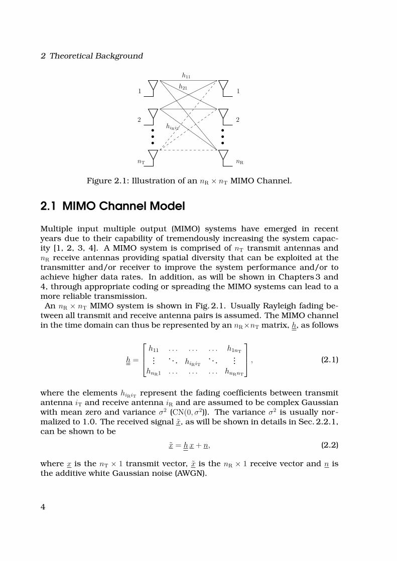
Figure 2.1: Illustration of an nR × nT MIMO Channel.
2.1 MIMO Channel Model
Multiple input multiple output (MIMO) systems have emerged in recentyears due to their capability of tremendously increasing the system capac-ity [1, 2, 3, 4]. A MIMO system is comprised of nT transmit antennas andnR receive antennas providing spatial diversity that can be exploited at thetransmitter and/or receiver to improve the system performance and/or toachieve higher data rates. In addition, as will be shown in Chapters 3 and4, through appropriate coding or spreading the MIMO systems can lead to amore reliable transmission.An nR × nT MIMO system is shown in Fig. 2.1. Usually Rayleigh fading be-
tween all transmit and receive antenna pairs is assumed. The MIMO channelin the time domain can thus be represented by an nR×nT matrix, h, as follows
h =
h11 . . . . . . . . . h1nT
.... . . hiRiT
. . ....
hnR1 . . . . . . . . . hnRnT
, (2.1)
where the elements hiRiT represent the fading coefficients between transmitantenna iT and receive antenna iR and are assumed to be complex Gaussianwith mean zero and variance σ2 (CN(0, σ2)). The variance σ2 is usually nor-malized to 1.0. The received signal x, as will be shown in details in Sec. 2.2.1,can be shown to be
x = hx + n, (2.2)
where x is the nT × 1 transmit vector, x is the nR × 1 receive vector and n isthe additive white Gaussian noise (AWGN).
4
2.2 Orthogonal Frequency Division Multiplexing
2.2 Orthogonal Frequency Division Multiplexing
Orthogonal frequency division multiplexing (OFDM) is a special case of fre-quency division multiplexing (FDM). The basic idea of OFDM is to dividethe available spectrum into several subchannels narrow enough that signalstransmitted over those subchannels experience flat fading. In addition, allof the subcarriers are transmitted simultaneously. As will be shown in thenext section, the subchannels are chosen such that they are orthogonal toeach other and thus no guard bands are required. In fact, the subchannelsare overlapping and the resulting channel is a sum of the narrow orthogonalsubchannels. OFDM is thus capable of achieving a high spectral efficiencywhile at the same time is able to combat multipath fading. The use of dis-crete Fourier transform (DFT) for modulation and demodulation, proposedby Weinstein and Ebert in 1971, eliminated the need for subcarrier oscilla-tors [5]. However, since Weinstein and Ebert only used a guard space betweenthe OFDM symbols, they could not obtain perfect orthogonality between thesubcarriers over multipath channels. In 1980, Peled and Ruiz were able tosolve the orthogonality problem by introducing the cyclic prefix (CP) to re-place the guard space. In the following section, we shall first describe SISO-OFDM using a CP and show its equivalent matrix vector transmission model.We then extend this model to the MIMO case. In all that follows, we shallassume that the channel is constant during one OFDM symbol duration.
2.2.1 SISO-OFDM
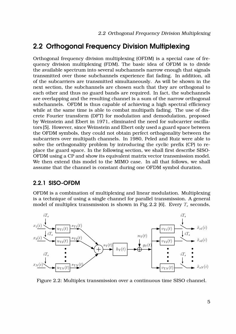
OFDM is a combination of multiplexing and linear modulation. Multiplexingis a technique of using a single channel for parallel transmission. A generalmodel of multiplex transmission is shown in Fig. 2.2 [6]. Every Ts seconds,
........
....
nT(t)
gT(t)sT(t)hT(t)
sT1(t)
sT2(t)
sTN(t)
x1(i)
x2(i)
xN(i)
uT1(t)
uT2(t)
uTN(t)
vT1(t)
vT2(t)
vTN(t)
iTs
iTs
iTsiTs
iTs
iTs
xo1(i)
xo2(i)
xoN(i)
Figure 2.2: Multiplex transmission over a continuous time SISO channel.
5
2 Theoretical Background
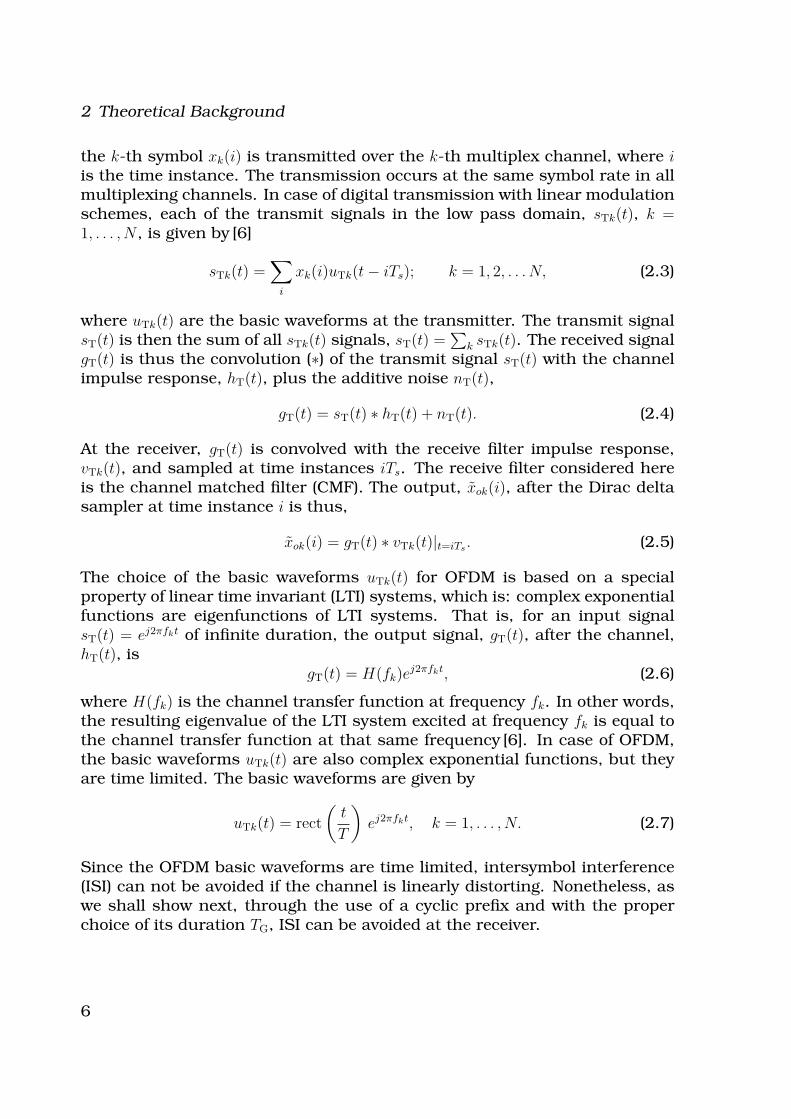
the k-th symbol xk(i) is transmitted over the k-th multiplex channel, where iis the time instance. The transmission occurs at the same symbol rate in allmultiplexing channels. In case of digital transmission with linear modulationschemes, each of the transmit signals in the low pass domain, sTk(t), k =1, . . . , N , is given by [6]
sTk(t) =∑
i
xk(i)uTk(t − iTs); k = 1, 2, . . . N, (2.3)
where uTk(t) are the basic waveforms at the transmitter. The transmit signalsT(t) is then the sum of all sTk(t) signals, sT(t) =
∑
k sTk(t). The received signalgT(t) is thus the convolution (∗) of the transmit signal sT(t) with the channelimpulse response, hT(t), plus the additive noise nT(t),
gT(t) = sT(t) ∗ hT(t) + nT(t). (2.4)
At the receiver, gT(t) is convolved with the receive filter impulse response,vTk(t), and sampled at time instances iTs. The receive filter considered hereis the channel matched filter (CMF). The output, xok(i), after the Dirac deltasampler at time instance i is thus,
xok(i) = gT(t) ∗ vTk(t)|t=iTs. (2.5)
The choice of the basic waveforms uTk(t) for OFDM is based on a specialproperty of linear time invariant (LTI) systems, which is: complex exponentialfunctions are eigenfunctions of LTI systems. That is, for an input signalsT(t) = ej2πfkt of infinite duration, the output signal, gT(t), after the channel,hT(t), is
gT(t) = H(fk)ej2πfkt, (2.6)
where H(fk) is the channel transfer function at frequency fk. In other words,the resulting eigenvalue of the LTI system excited at frequency fk is equal tothe channel transfer function at that same frequency [6]. In case of OFDM,the basic waveforms uTk(t) are also complex exponential functions, but theyare time limited. The basic waveforms are given by
uTk(t) = rect
(
t
T
)
ej2πfkt, k = 1, . . . , N. (2.7)
Since the OFDM basic waveforms are time limited, intersymbol interference(ISI) can not be avoided if the channel is linearly distorting. Nonetheless, aswe shall show next, through the use of a cyclic prefix and with the properchoice of its duration TG, ISI can be avoided at the receiver.
6
2.2 Orthogonal Frequency Division Multiplexing
s(t), first path
s(t−τ1), second path
Output of Two Path Channel
s(t), first path
s(t−τ2), second path
Output of Two Path Channel
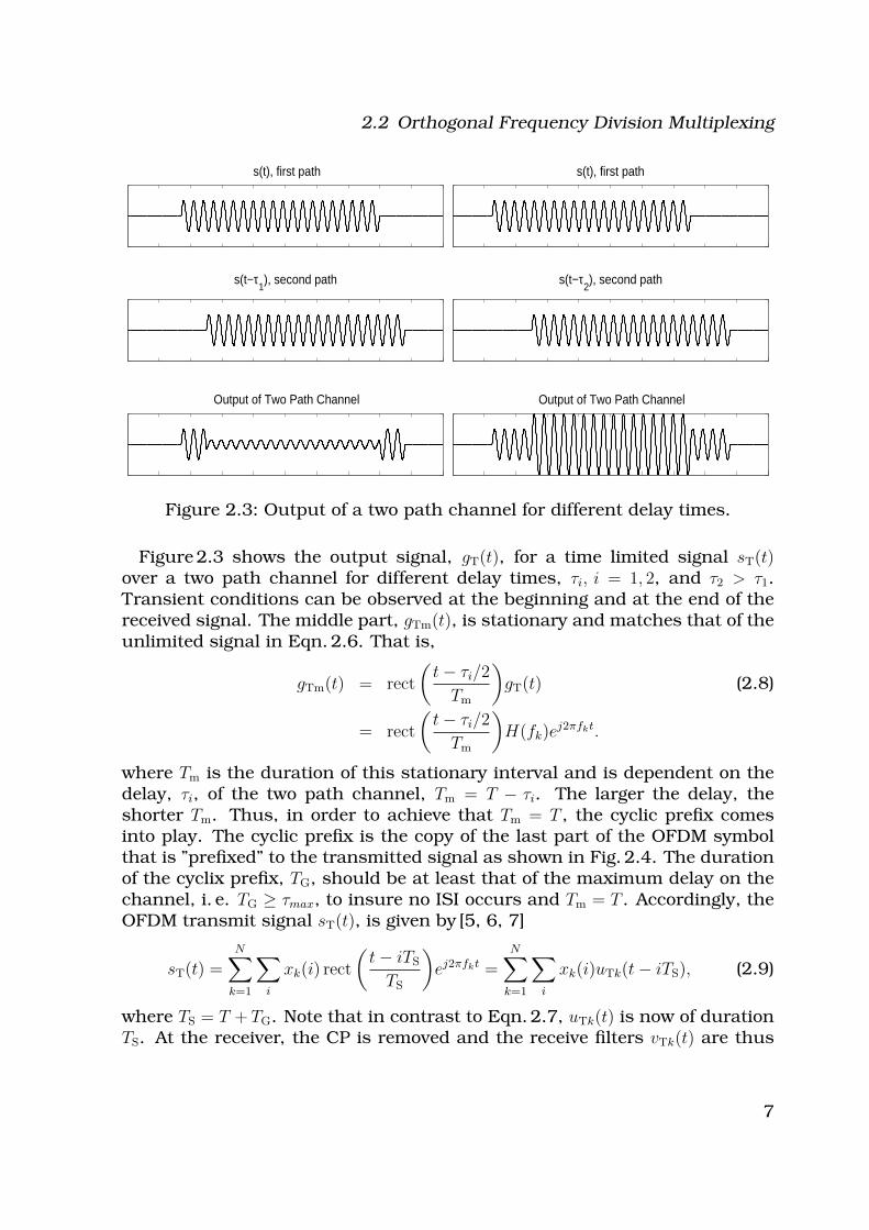
Figure 2.3: Output of a two path channel for different delay times.
Figure 2.3 shows the output signal, gT(t), for a time limited signal sT(t)over a two path channel for different delay times, τi, i = 1, 2, and τ2 > τ1.Transient conditions can be observed at the beginning and at the end of thereceived signal. The middle part, gTm(t), is stationary and matches that of theunlimited signal in Eqn. 2.6. That is,
gTm(t) = rect
(
t − τi/2
Tm
)
gT(t) (2.8)
= rect
(
t − τi/2
Tm
)
H(fk)ej2πfkt.
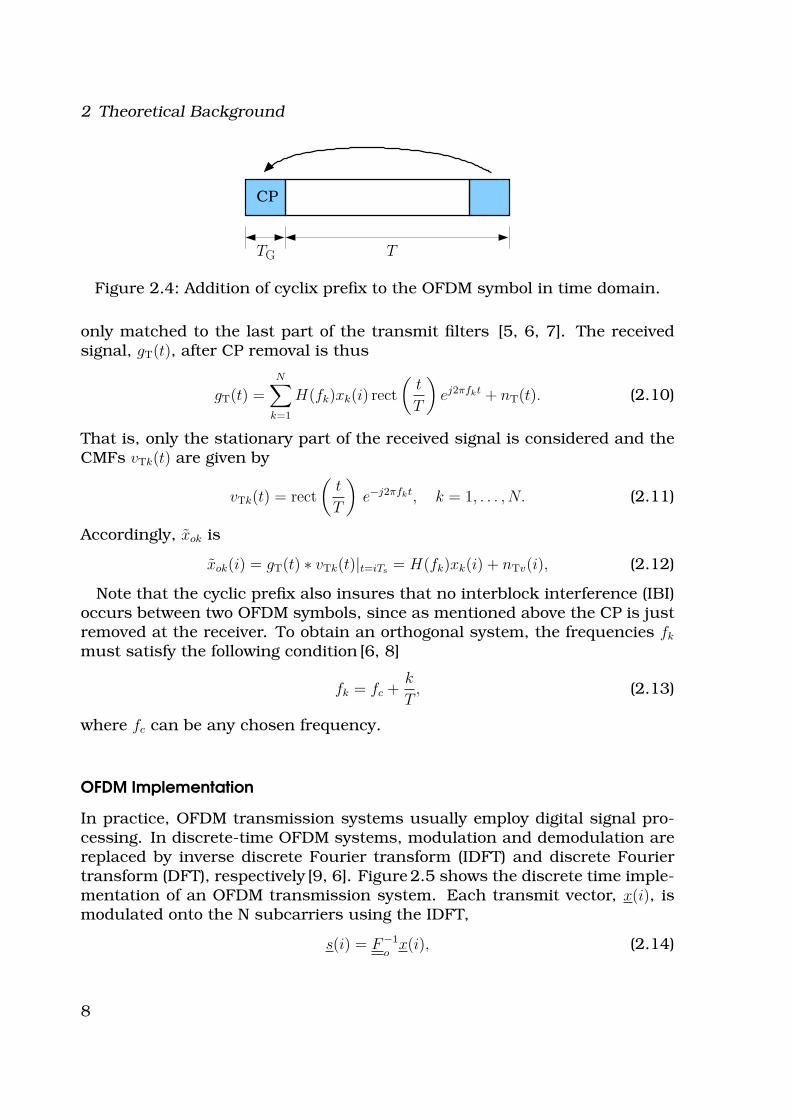
where Tm is the duration of this stationary interval and is dependent on thedelay, τi, of the two path channel, Tm = T − τi. The larger the delay, theshorter Tm. Thus, in order to achieve that Tm = T , the cyclic prefix comesinto play. The cyclic prefix is the copy of the last part of the OFDM symbolthat is ”prefixed” to the transmitted signal as shown in Fig. 2.4. The durationof the cyclix prefix, TG, should be at least that of the maximum delay on thechannel, i. e. TG ≥ τmax, to insure no ISI occurs and Tm = T . Accordingly, theOFDM transmit signal sT(t), is given by [5, 6, 7]
sT(t) =N∑
k=1
∑
i
xk(i) rect
(
t − iTS
TS
)
ej2πfkt =N∑
k=1
∑
i
xk(i)uTk(t − iTS), (2.9)
where TS = T + TG. Note that in contrast to Eqn. 2.7, uTk(t) is now of durationTS. At the receiver, the CP is removed and the receive filters vTk(t) are thus
7
2 Theoretical Background
CP
TG T
Figure 2.4: Addition of cyclix prefix to the OFDM symbol in time domain.
only matched to the last part of the transmit filters [5, 6, 7]. The receivedsignal, gT(t), after CP removal is thus
gT(t) =N∑
k=1
H(fk)xk(i) rect
(
t
T
)
ej2πfkt + nT(t). (2.10)
That is, only the stationary part of the received signal is considered and theCMFs vTk(t) are given by
vTk(t) = rect
(
t
T
)
e−j2πfkt, k = 1, . . . , N. (2.11)
Accordingly, xok is
xok(i) = gT(t) ∗ vTk(t)|t=iTs = H(fk)xk(i) + nTv(i), (2.12)
Note that the cyclic prefix also insures that no interblock interference (IBI)occurs between two OFDM symbols, since as mentioned above the CP is justremoved at the receiver. To obtain an orthogonal system, the frequencies fk
must satisfy the following condition [6, 8]
fk = fc +k
T, (2.13)
where fc can be any chosen frequency.
OFDM Implementation
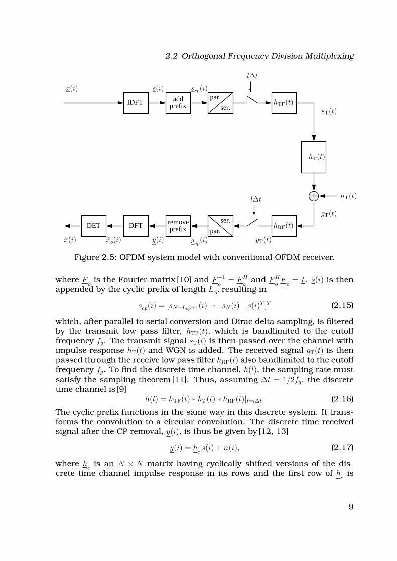
In practice, OFDM transmission systems usually employ digital signal pro-cessing. In discrete-time OFDM systems, modulation and demodulation arereplaced by inverse discrete Fourier transform (IDFT) and discrete Fouriertransform (DFT), respectively [9, 6]. Figure 2.5 shows the discrete time imple-mentation of an OFDM transmission system. Each transmit vector, x(i), ismodulated onto the N subcarriers using the IDFT,
s(i) = F−1
ox(i), (2.14)
8
2.2 Orthogonal Frequency Division Multiplexing
IDFT prefix
removeprefix
add
DFT
par.
ser.
par.DET
ser.
nT(t)
gT(t)
sT(t)
hT(t)
yT(t)
s(i) scp(i)
y(i) ycp
(i)
hTF(t)
hRF(t)
xo(i)x(i)
x(i)
l∆t
l∆t
Figure 2.5: OFDM system model with conventional OFDM receiver.
where Fo
is the Fourier matrix [10] and F−1
o= FH
oand FH
oF
o= I. s(i) is then
appended by the cyclic prefix of length Lcp resulting in
scp(i) = [sN−Lcp+1(i) · · · sN(i) s(i)T ]T (2.15)
which, after parallel to serial conversion and Dirac delta sampling, is filteredby the transmit low pass filter, hTF(t), which is bandlimited to the cutofffrequency fg. The transmit signal sT(t) is then passed over the channel withimpulse response hT(t) and WGN is added. The received signal gT(t) is thenpassed through the receive low pass filter hRF(t) also bandlimited to the cutofffrequency fg. To find the discrete time channel, h(l), the sampling rate mustsatisfy the sampling theorem [11]. Thus, assuming ∆t = 1/2fg, the discretetime channel is [9]
h(l) = hTF(t) ∗ hT (t) ∗ hRF(t)|t=l∆t. (2.16)
The cyclic prefix functions in the same way in this discrete system. It trans-forms the convolution to a circular convolution. The discrete time receivedsignal after the CP removal, y(i), is thus be given by [12, 13]
y(i) = hcs(i) + n(i), (2.17)
where hc
is an N × N matrix having cyclically shifted versions of the dis-crete time channel impulse response in its rows and the first row of h
cis
9
2 Theoretical Background
......
n1
x1
H1
xo1
n2
x2
H2
xo2
nN
xN
HN
xoN
(a) Parallel SISO-OFDMsubcarriers
n
x xoH
(b) Equivalent matrix vector trans-mission model
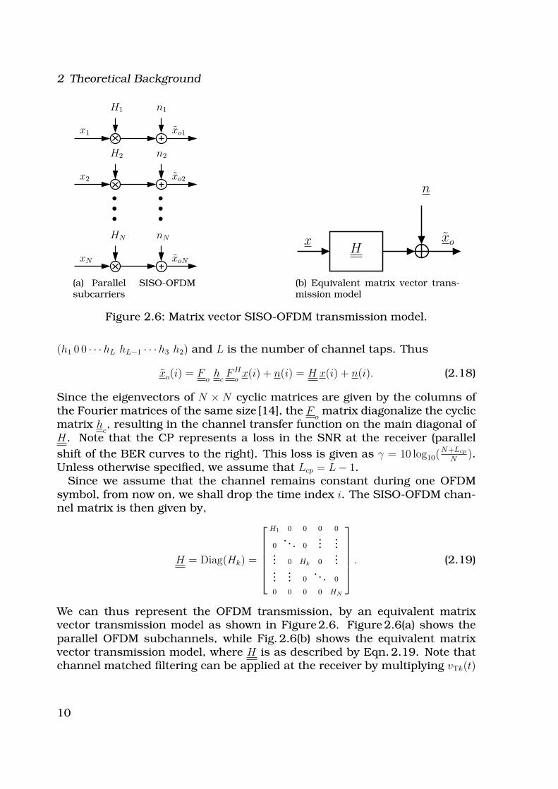
Figure 2.6: Matrix vector SISO-OFDM transmission model.
(h1 0 0 · · ·hL hL−1 · · ·h3 h2) and L is the number of channel taps. Thus
xo(i) = Fo
hcFH
ox(i) + n(i) = H x(i) + n(i). (2.18)
Since the eigenvectors of N × N cyclic matrices are given by the columns ofthe Fourier matrices of the same size [14], the F
omatrix diagonalize the cyclic
matrix hc, resulting in the channel transfer function on the main diagonal of
H. Note that the CP represents a loss in the SNR at the receiver (parallel
shift of the BER curves to the right). This loss is given as γ = 10 log10(N+Lcp
N).
Unless otherwise specified, we assume that Lcp = L − 1.Since we assume that the channel remains constant during one OFDM
symbol, from now on, we shall drop the time index i. The SISO-OFDM chan-nel matrix is then given by,
H = Diag(Hk) =
H1 0 0 0 0
0... 0
......
... 0 Hk 0...
...... 0
... 0
0 0 0 0 HN
. (2.19)
We can thus represent the OFDM transmission, by an equivalent matrixvector transmission model as shown in Figure 2.6. Figure 2.6(a) shows theparallel OFDM subchannels, while Fig. 2.6(b) shows the equivalent matrixvector transmission model, where H is as described by Eqn. 2.19. Note thatchannel matched filtering can be applied at the receiver by multiplying vTk(t)
10
2.2 Orthogonal Frequency Division Multiplexing
1 2 3 4 5 6 7 8
1
2
3
4
5
6
7
8
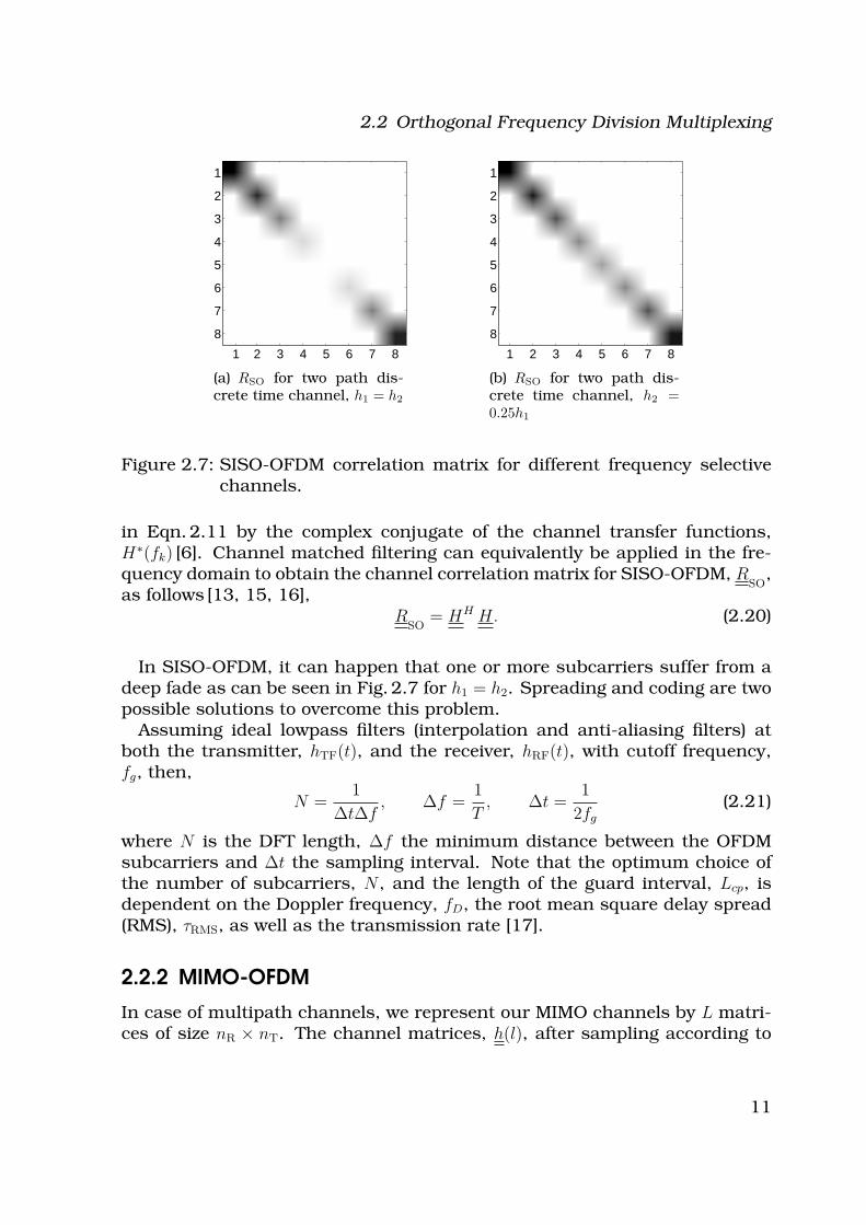
(a) RSO for two path dis-crete time channel, h1 = h2
1 2 3 4 5 6 7 8
1
2
3
4
5
6
7
8
(b) RSO for two path dis-crete time channel, h2 =0.25h1
Figure 2.7: SISO-OFDM correlation matrix for different frequency selectivechannels.
in Eqn. 2.11 by the complex conjugate of the channel transfer functions,H∗(fk) [6]. Channel matched filtering can equivalently be applied in the fre-quency domain to obtain the channel correlation matrix for SISO-OFDM, R
SO,
as follows [13, 15, 16],R
SO= HH H. (2.20)
In SISO-OFDM, it can happen that one or more subcarriers suffer from adeep fade as can be seen in Fig. 2.7 for h1 = h2. Spreading and coding are twopossible solutions to overcome this problem.
Assuming ideal lowpass filters (interpolation and anti-aliasing filters) atboth the transmitter, hTF(t), and the receiver, hRF(t), with cutoff frequency,fg, then,
N =1
∆t∆f, ∆f =
1
T, ∆t =
1
2fg
(2.21)
where N is the DFT length, ∆f the minimum distance between the OFDMsubcarriers and ∆t the sampling interval. Note that the optimum choice ofthe number of subcarriers, N , and the length of the guard interval, Lcp, isdependent on the Doppler frequency, fD, the root mean square delay spread(RMS), τRMS, as well as the transmission rate [17].
2.2.2 MIMO-OFDM
In case of multipath channels, we represent our MIMO channels by L matri-ces of size nR × nT. The channel matrices, h(l), after sampling according to
11
2 Theoretical Background
par.
ser.
par.
ser.
111 1 11 1
DFT
1
1 1
DFT
1
1 1
DFT
1
Spre
adin
g
IDFT
1add
IDFT
1 1add
prefix
IDFT
1 1add
prefix
1
1
par.
ser.prefix
Rec
eive
r
Join
t Det
ectio
n
ser.
par.
remove
prefix
ser.
par.
remove
prefix
ser.
par.
remove
prefix
MIMO Channel
x xx
Tx1
Tx2
TxnT NnTNnTNnT NN
NN
N
NN
NN
NNN
N+Lcp
N+Lcp
N+Lcp
N+Lcp
N+LcpN+Lcp
CM
Fan
dD
espre
adin
g
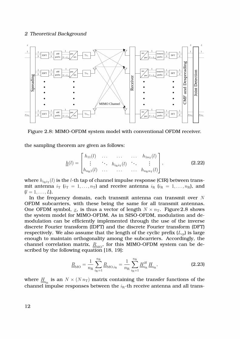
Figure 2.8: MIMO-OFDM system model with conventional OFDM receiver.
the sampling theorem are given as follows:
h(l) =
h11(l) . . . . . . . . . h1nT(l)
.... . . hiRiT(l)
. . ....
hnR1(l) . . . . . . . . . hnRnT(l)
, (2.22)
where hiRiT(l) is the l-th tap of channel impulse response (CIR) between trans-mit antenna iT (iT = 1, . . . , nT) and receive antenna iR (iR = 1, . . . , nR), and(l = 1, . . . , L).
In the frequency domain, each transmit antenna can transmit over NOFDM subcarriers, with these being the same for all transmit antennas.One OFDM symbol, x, is thus a vector of length N × nT. Figure 2.8 showsthe system model for MIMO-OFDM. As in SISO-OFDM, modulation and de-modulation can be efficiently implemented through the use of the inversediscrete Fourier transform (IDFT) and the discrete Fourier transform (DFT)respectively. We also assume that the length of the cyclic prefix (Lcp) is largeenough to maintain orthogonality among the subcarriers. Accordingly, thechannel correlation matrix, R
MO, for this MIMO-OFDM system can be de-
scribed by the following equation [18, 19]:
RMO
=1
nR
nR∑
iR=1
RMO,iR
=1
nR
nR∑
iR=1
HH
iRH
iR, (2.23)
where HiR
is an N × (N nT) matrix containing the transfer functions of the
channel impulse responses between the iR-th receive antenna and all trans-
12

2.2 Orthogonal Frequency Division Multiplexing
mit antennas, HiR
= [HiR1
, . . . , HiRnT
], where (·)H denotes the complex conju-
gate transpose operation also known as Hermitian. The submatrices HiRiT
are N × N diagonal matrices and are given by:
HiRiT
= Diag(DFT(hiRiT)) =
HiRiT(1) 0 0 0 0
0... 0
......
... 0 HiRiT(k) 0
......
... 0... 0
0 0 0 0 HiRiT(N)
, . (2.24)
where hiRiT= [hiRiT(1), . . . , hiRiT(l), . . . , hiRiT(L)] and represents the channel im-
pulse response (CIR) between transmit antenna iT and receive antenna iR,and L is the maximum number of taps. DFT stands for the discrete Fouriertransform and accordingly HiRiT(k) is the transfer function at frequency k,k = 1, . . . , N for the channel between transmit antenna iT and receive an-tenna iR .The channel correlation matrix, R
MO, can alternatively be described by the
following equation [19, 18]:
RMO
=1
nR
HH H, (2.25)
where H is an (N nR) × (N nT) matrix containing the transfer functions of thechannel impulse responses between all receive and transmit antennas. H isgiven by
H =
H11
. . . . . . . . . H1nT
.... . . H
iRiT
. . ....
HnR1
. . . . . . . . . HnRnT
, (2.26)
where iT = 1 . . . nT and iR = 1 . . . nR. The submatrices HiRiT
are N ×N diagonal
matrices and are also given by Eqn. 2.24. Note that the diagonal elements,rii, of R
MOare always positive and contain the receive diversity. The diagonal
elements are given by rii = 1/nR
∑nR
iR=1 H∗iRiT
(k)HiRiT(k), where i represents thediagonal element belonging to transmit antenna iT and frequency k. Thisweighted sum over all receive antennas obtained through the use of the CMF(Eqns. 2.25 and 2.23) is also known as maximum ration combining (MRC) [6].The MRC operation maximizes the SNR if the channel is perfectly known atthe receiver [20].
Figure 2.9 shows the matrix vector transmission model for MIMO-OFDM.The channel matrices, H, unlike for SISO-OFDM are not diagonal matrices.Intersymbol interference occurs between symbols that are transmitted from
13
2 Theoretical Background
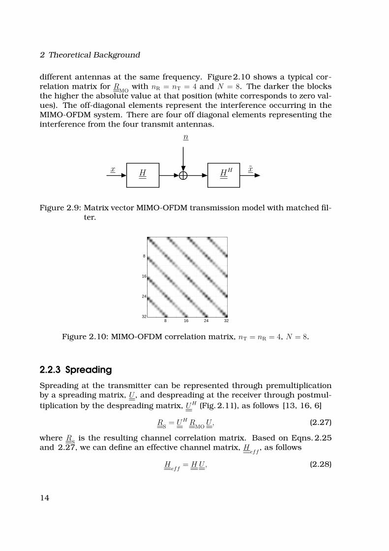
different antennas at the same frequency. Figure 2.10 shows a typical cor-relation matrix for R
MOwith nR = nT = 4 and N = 8. The darker the blocks
the higher the absolute value at that position (white corresponds to zero val-ues). The off-diagonal elements represent the interference occurring in theMIMO-OFDM system. There are four off diagonal elements representing theinterference from the four transmit antennas.
n
x xH HH
Figure 2.9: Matrix vector MIMO-OFDM transmission model with matched fil-ter.
8 16 24 32
8
16
24
32
Figure 2.10: MIMO-OFDM correlation matrix, nT = nR = 4, N = 8.
2.2.3 Spreading
Spreading at the transmitter can be represented through premultiplicationby a spreading matrix, U , and despreading at the receiver through postmul-
tiplication by the despreading matrix, UH (Fig. 2.11), as follows [13, 16, 6]
RS
= UH RMO
U, (2.27)
where RS
is the resulting channel correlation matrix. Based on Eqns. 2.25and 2.27, we can define an effective channel matrix, H
eff, as follows
Heff
= H U, (2.28)
14
2.2 Orthogonal Frequency Division Multiplexing
eplacements
n
x xH HHU UH
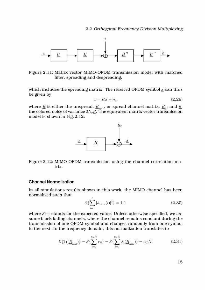
Figure 2.11: Matrix vector MIMO-OFDM transmission model with matchedfilter, spreading and despreading.
which includes the spreading matrix. The received OFDM symbol x can thusbe given by
x = R x + nc, (2.29)
where R is either the unspread, RMO
, or spread channel matrix, RS, and nc
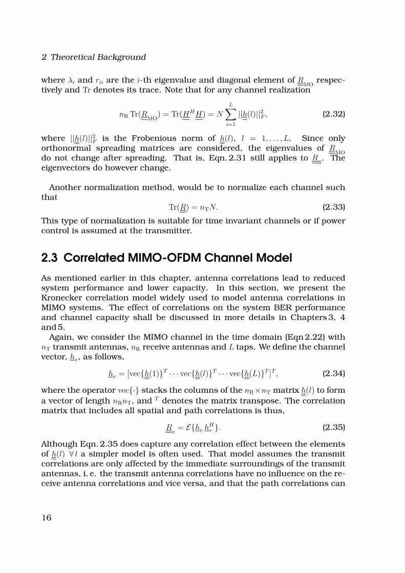
the colored noise of variance 2NoR. The equivalent matrix vector transmissionmodel is shown in Fig. 2.12.
nc
x xR
Figure 2.12: MIMO-OFDM transmission using the channel correlation ma-trix.
Channel Normalization
In all simulations results shown in this work, the MIMO channel has beennormalized such that
E{L∑
i=1
|hiRiT(l)|2} = 1.0, (2.30)
where E{·} stands for the expected value. Unless otherwise specified, we as-sume block fading channels, where the channel remains constant during thetransmission of one OFDM symbol and changes randomly from one symbolto the next. In the frequency domain, this normalization translates to
E{Tr(RMO
)} = E{nTN∑
i=1
rii} = E{nTN∑
i=1
λi(RMO)} = nTN, (2.31)
15
2 Theoretical Background
where λi and rii are the i-th eigenvalue and diagonal element of RMO
respec-tively and Tr denotes its trace. Note that for any channel realization
nR Tr(RMO
) = Tr(HHH) = N
L∑
i=1
||h(l)||2F , (2.32)
where ||h(l)||2F is the Frobenious norm of h(l), l = 1, . . . , L. Since onlyorthonormal spreading matrices are considered, the eigenvalues of R
MOdo not change after spreading. That is, Eqn. 2.31 still applies to R
S. The
eigenvectors do however change.
Another normalization method, would be to normalize each channel suchthat
Tr(R) = nTN. (2.33)
This type of normalization is suitable for time invariant channels or if powercontrol is assumed at the transmitter.
2.3 Correlated MIMO-OFDM Channel Model
As mentioned earlier in this chapter, antenna correlations lead to reducedsystem performance and lower capacity. In this section, we present theKronecker correlation model widely used to model antenna correlations inMIMO systems. The effect of correlations on the system BER performanceand channel capacity shall be discussed in more details in Chapters 3, 4and 5.
Again, we consider the MIMO channel in the time domain (Eqn 2.22) withnT transmit antennas, nR receive antennas and L taps. We define the channelvector, hv, as follows,
hv = [vec{h(1)}T · · · vec{h(l)}T · · · vec{h(L)}T ]T , (2.34)
where the operator vec{·} stacks the columns of the nR×nT matrix h(l) to form
a vector of length nRnT, and T denotes the matrix transpose. The correlationmatrix that includes all spatial and path correlations is thus,
Rv
= E{hv hHv }. (2.35)
Although Eqn. 2.35 does capture any correlation effect between the elementsof h(l) ∀ l a simpler model is often used. That model assumes the transmitcorrelations are only affected by the immediate surroundings of the transmitantennas, i. e. the transmit antenna correlations have no influence on the re-ceive antenna correlations and vice versa, and that the path correlations can
16
2.3 Correlated MIMO-OFDM Channel Model
be separated from spatial correlations, the correlation matrix in Eqn. 2.35can be expressed by the Kronecker product of the transmit, receive and pathcorrelations as follows [21],
Rv
= kP⊗ kT
T(1) ⊗ k
R(1), (2.36)
where kP
is the path correlation, kT(1), k
R(1) transmit and receive correla-
tions at the non-delay tap l = 1 respectively. This correlation model is wellknown as the Kronecker correlation model [21, 22]. If, in addition, we as-sume an equal power delay profile (PDP) and no path correlations (i. e. thedifferent channel taps fade independently), k
P= I, the correlation matrix R
vin Eqn. 2.36 becomes
Rv
= I ⊗ kT
T(1) ⊗ k
R(1) (2.37)
If correlation matrices of the other channel taps are to be taken into consid-eration, again assuming uncorrelated paths and equal PDP,
Rv
= BlkDiag([Rkv
(1) · · ·Rkv
(l) · · ·Rkv
(L)]), (2.38)
where Rkv
(l) = kT(l)T ⊗ k
R(l), and BlkDiag forms a block diagonal matrix with
the matrices Rk(l) on the main diagonal. Based on the Kronecker correlation
model described above, the correlated channel matrices, hc(l), can thus bemodeled as follows [21, 22],
hc(l) = k1/2
R(l)h(l)k1/2
T(l), (2.39)
where kR(l) = k1/2
R(l)k1/2
R(l) and k
T(l) = k1/2
T(l)k1/2
T(l) are the nR × nR receive
and nT × nT transmit correlation matrices for the l-th tap respectively. Thetransmit and receive correlation matrices can be calculated as follows,
kT(l) = 1
nRE{h(l)Hh(l)}, (2.40)
kR(l) = 1
nTE{h(l)h(l)H}. (2.41)
If we assume that the transmit and receive correlation matrices are thesame for all taps, i. e.,
k(l) = k1/2(l)k1/2(l) = k1/2k1/2 = k, (2.42)
where k is either the transmit or receive correlation matrix, then Rv inEqn. 2.38 simplifies to R
v= I ⊗ k
T⊗ k
R.
Since the correlation matrices are positive definite, the eigenvalue decom-position was used to calculate the square root of the correlation matrices asfollows,
k = v e vH ,
k1/2 = v e1/2 vH . (2.43)
17
2 Theoretical Background
v is a matrix containing the eigenvectors of k and e is a diagonal matrixcontaining its eigenvalues. The square root of a diagonal matrix is simplythe square root of its diagonal elements. Thus, Hc is then simply calculatedby replacing hiRiT
by hciRiT
in Eqn. 2.24, i. e. Hc
iRiT= diag[DFT(hc
iRiT)]. In other
words, the correlated channel matrices in Eqn. 2.39 are used instead ofEqn. 2.22 to obtain H in Eqn. 2.26.
Antenna Correlation Models
We assume linear antenna arrays with uniformly spaced antennas at boththe transmitter and receiver. Antennas at the same distance m are also as-sumed to experience the same correlations. Thus, k
Rand k
Ttake the follow-
ing form,
1 c12 c13 · · · c1n
c21 1 c23 · · · c2n
c31 c32 1 ..cij.. :: : : : :: ..cji.. : : :
cn1 . . . . . . . . . 1
=
1 ρ1 ρ2 · · · ρn−1
ρ∗1 1 ρ1 · · · ρn−2
ρ∗2 ρ∗
1 1 ..ρm.. :: : : : :: ..ρ∗
m.. : : :ρ∗
n−1 . . . . . . . . . 1
, (2.44)
where n is either nR or nT, cii = 1 and cij = ρj−i for j > i and cji = c∗ij for j < i(i = 1, . . . , n, j = 1, . . . , n). Accordingly, ρm is the correlation coefficient betweenantennas with spacing m = |j−i|. Throughout this work, we shall concentrateon two correlation models: constant and exponential correlation model. Forthe constant correlation model, the correlation coefficients are real and thesame for all antennas, i. e. ρm = ρ ∀m and |ρ| < 1. For the exponentialcorrelation model, the correlation coefficients are defined as follows [23],
cij = ρm = ρj−i ∀ i ≤ j (2.45)
cji = c∗ij,
for real coefficients ρ, |ρ| < 1 and
cij = ρm = (ρ +√−1 ρ)j−i ∀ i ≤ j (2.46)
cji = c∗ij,
for complex coefficients ρ +√−1 ρ. Note that |ρ +
√−1 ρ| < 1 for the corre-
lation matrix to remain positive definite. Another example of a widely usedcorrelation matrix is the tridiagonal correlation matrix [24]. The correlationmatrix is given by Eqn. 2.44 where ρm = ρ ∀m ≤ M and ρm = 0 otherwiseand M < n.
18
2.4 Effect of Antenna Correlations
2.4 Effect of Antenna Correlations
In this section, we introduce three different measures that show how antennacorrelations can affect the performance of the MIMO system.
2.4.1 Channel Condition Number
The condition number, χ, is defined as the ratio between the maximum, λmax,and the minimum, λmin, eigenvalue of a matrix [25].
χ =λmax
λmin
(2.47)
If λi = 1 ∀i, then the matrix is an identity matrix. A singular matrix has aCN = ∞, since λmin = 0. That is, the higher the condition number, the moresingular the channel correlation matrix gets and worse BER performance isto be expected. As will be shown in Chapter 3, increasing the antenna cor-relations leads to higher condition numbers and accordingly to deterioratingperformance.
2.4.2 Diversity and Correlation Measures
Definition 1 For a flat fading channel, the diversity measure of Rv, Ψ(R
v),
was first introduced in [26, 27] and is given by
Ψ(Rv) =
(
Tr(Rv)
||Rv||F
)2
=
( ∑Mi=1 λi
√
∑Mi=1 λ2
i
)2
(2.48)
where Rv
= E{hvhHv } is an M × M (M = nTnR) matrix, hv = vec{h} and λi is the
ith eigenvalue of Rv. Ψ(R
v) is bound by [26]
1 ≤ Ψ(Rv) ≤ M (2.49)
An important property of the diversity measure is, if the first n eigenvaluesof R
vare identical (i. e. λ1 = λ2, · · · , = λn) and the remaining eigenvalues are
zeros, then Ψ = n. That is, the correlation measure becomes equal to therank of R
v. If the nonzero eigenvalues of R
vare not equal, Ψ < n which can
be interpreted as the number of dominant eigenvalues [27, 28]. That is, thediversity measure gives the number of dominant eigenvalues of R
vand not its
rank. The rank of Rv
is always equal to M as long as the correlation matriceshave full rank. rank(R
v) = 1 if and only if the channel is fully correlated. For
Rv
= 1 (1 is an all one matrix), the diversity measure is 1, while for Rv
= I,
19
2 Theoretical Background
the diversity measure is M. Accordingly, the larger the spread the lower thediversity measure.
According to the correlation model given in Sec. 2.3, Rv
for a flat fadingchannel (L = 1) is given by
Rv
= kT⊗ k
R. (2.50)
Consequently, from Appendix A.2.1, the rank Rv
= rank kT· rank k
R, and R
vremains full rank as long as both k
Tand k
Rare full rank. The diversity
measure can accordingly also be expressed by [26]
Ψ(Rv) = Ψ(k
T)Ψ(k
R), (2.51)
where Ψ(kT) and Ψ(k
R) are the transmit and receive diversity measures re-
spectively.
Definition 2 In [26, 27], the correlation measure was also defined, Φ(k) for
an n × n correlation matrix k
Φ(k) =
√
n/Ψ(k) − 1
n − 1(2.52)
which can be used as a measure for the amount of correlation present.
The correlation measure is especially useful if different correlation modelsare compared. Φ(k) ranges between 0.0 (all equal eigenvalues: uncorrelated)and 1.0 (rank one correlation matrix: full correlation). It is also worth notinghere, that the correlation measure for the constant correlation model isΦ(k) = ρ.
In case of frequency selective channels, we look at the channel in the fre-quency domain. The diversity measure is the sum of the diversity measuresof the uncorrelated subcarriers when using OFDM. Then the diversity mea-sure can be calculated as follows,
Ψ(Rv) =
Nc∑
k=1
Ψ(Rvk
)
where Nc is the number of coherence bandwidth, and Ψ(Rvk
) is the diversity
measure calculated at each coherence bandwidth. If we assume the sameantenna correlations at each frequency, and independent and uncorrelatedfading of the channel taps of equal power delay profile then
Ψ(Rv) = L Ψ(R
vk), (2.53)
20

2.4 Effect of Antenna Correlations
where Ψ(Rvk
) is the diversity measure at any frequency k, Rvk
=
E{vec{Hk} vec{H
k}H}, H
kis the nR × nT channel frequency response at fre-
quency k and L is the number of channel taps. Thus, in case of a frequencyselective channel, the diversity measure is bound by
L ≤ Ψ(Rv) ≤ LM, (2.54)
where M = nTnR.
0 0.2 0.4 0.6 0.8 11
1.5
2
2.5
3
3.5
4
ρ
Ψ(k
)
constexpcomplex exp
(a) Diversity Measure Ψ(k)
0 0.2 0.4 0.6 0.8 11
4
7
10
13
16
ρ
Ψ(k
R)Ψ
(kT)
constexpcomplex exp
(b) Diversity Measure Ψ(kT)Ψ(k
R)
Figure 2.13: Diversity measure versus ρ for 4 × 4 constant, exponential andcomplex exponential correlation matrices.
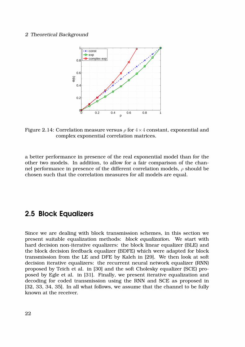
Figures 2.13 and 2.14 show the diversity and correlation measures for thethree previously described correlation matrices of size 4 × 4. Figure 2.13(a)shows the diversity measure in presence of transmit correlations only andFig.2.13(b) in presence of both transmit and receive correlations. It is shownin Appendix 3.A.2, that the higher the antenna correlations, the wider theeigenvalue spread and accordingly, the lower the diversity measure. The di-versity measure is lower if both transmit and receive correlations exist thanif only one or the other is present since a larger eigenvalue spread is expectedfor the former case. The real exponential correlation matrix has the highestdiversity measure and lowest correlation measure for a given ρ. The constantand complex exponential correlation matrices have comparable diversity andcorrelation measure values for ρ ≤ 0.4. The complex exponential reachesits highest correlation measure (1.0) for ρ ≈ 0.7 (i. e. |c| = 1). The diversityand correlation measures therefore give an indication of the expected systemperformance. The higher the correlation measure and the lower the diversitymeasure the worse the expected performance. Thus, for a given ρ, we expect
21
2 Theoretical Background
0 0.2 0.4 0.6 0.8 10
0.2
0.4
0.6
0.8
1
ρ
Φ(k
)
constexpcomplex exp
Figure 2.14: Correlation measure versus ρ for 4×4 constant, exponential andcomplex exponential correlation matrices.
a better performance in presence of the real exponential model than for theother two models. In addition, to allow for a fair comparison of the chan-nel performance in presence of the different correlation models, ρ should bechosen such that the correlation measures for all models are equal.
2.5 Block Equalizers
Since we are dealing with block transmission schemes, in this section wepresent suitable equalization methods: block equalization. We start withhard decision non-iterative equalizers: the block linear equalizer (BLE) andthe block decision feedback equalizer (BDFE) which were adapted for blocktransmission from the LE and DFE by Kaleh in [29]. We then look at softdecision iterative equalizers: the recurrent neural network equalizer (RNN)proposed by Teich et al. in [30] and the soft Cholesky equalizer (SCE) pro-posed by Egle et al. in [31]. Finally, we present iterative equalization anddecoding for coded transmission using the RNN and SCE as proposed in[32, 33, 34, 35]. In all what follows, we assume that the channel to be fullyknown at the receiver.
22
2.5 Block Equalizers
x x xo
Θ(·)G
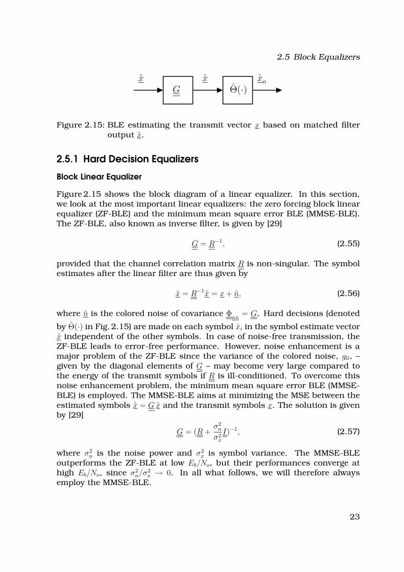
Figure 2.15: BLE estimating the transmit vector x based on matched filteroutput x.
2.5.1 Hard Decision Equalizers
Block Linear Equalizer
Figure 2.15 shows the block diagram of a linear equalizer. In this section,we look at the most important linear equalizers: the zero forcing block linearequalizer (ZF-BLE) and the minimum mean square error BLE (MMSE-BLE).The ZF-BLE, also known as inverse filter, is given by [29]
G = R−1, (2.55)
provided that the channel correlation matrix R is non-singular. The symbolestimates after the linear filter are thus given by
x = R−1x = x + n, (2.56)
where n is the colored noise of covariance Φnn
= G. Hard decisions (denoted
by Θ(·) in Fig. 2.15) are made on each symbol xi in the symbol estimate vectorx independent of the other symbols. In case of noise-free transmission, theZF-BLE leads to error-free performance. However, noise enhancement is amajor problem of the ZF-BLE since the variance of the colored noise, gll, –given by the diagonal elements of G – may become very large compared tothe energy of the transmit symbols if R is ill-conditioned. To overcome thisnoise enhancement problem, the minimum mean square error BLE (MMSE-BLE) is employed. The MMSE-BLE aims at minimizing the MSE between theestimated symbols x = G x and the transmit symbols x. The solution is givenby [29]
G = (R +σ2
n
σ2x
I)−1, (2.57)
where σ2n is the noise power and σ2
x is symbol variance. The MMSE-BLEoutperforms the ZF-BLE at low Eb/No, but their performances converge athigh Eb/No, since σ2
n/σ2x → 0. In all what follows, we will therefore always
employ the MMSE-BLE.
23
2 Theoretical Background
.x x xoxf
xb
Θ(·)
Gb
Gf
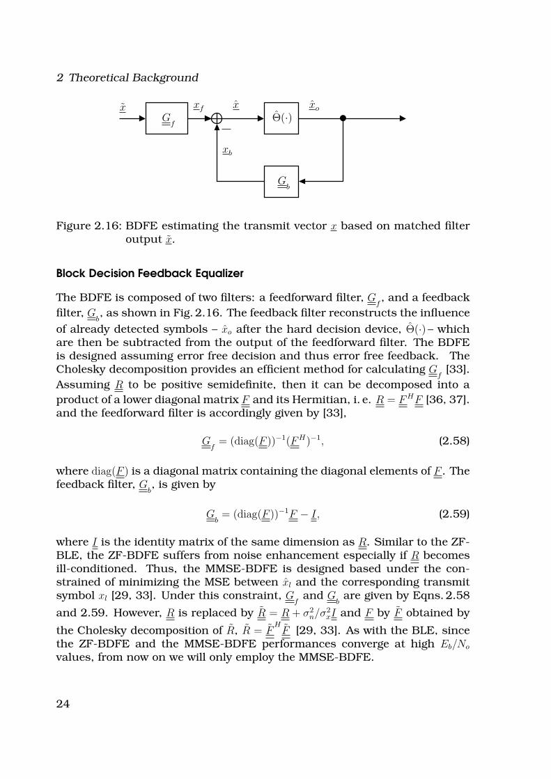
Figure 2.16: BDFE estimating the transmit vector x based on matched filteroutput x.
Block Decision Feedback Equalizer
The BDFE is composed of two filters: a feedforward filter, Gf, and a feedback
filter, Gb, as shown in Fig. 2.16. The feedback filter reconstructs the influence
of already detected symbols – xo after the hard decision device, Θ(·) – whichare then be subtracted from the output of the feedforward filter. The BDFEis designed assuming error free decision and thus error free feedback. TheCholesky decomposition provides an efficient method for calculating G
f[33].
Assuming R to be positive semidefinite, then it can be decomposed into a
product of a lower diagonal matrix F and its Hermitian, i. e. R = FHF [36, 37].and the feedforward filter is accordingly given by [33],
Gf
= (diag(F ))−1(FH)−1, (2.58)
where diag(F ) is a diagonal matrix containing the diagonal elements of F . Thefeedback filter, G
b, is given by
Gb= (diag(F ))−1F − I, (2.59)
where I is the identity matrix of the same dimension as R. Similar to the ZF-BLE, the ZF-BDFE suffers from noise enhancement especially if R becomesill-conditioned. Thus, the MMSE-BDFE is designed based under the con-strained of minimizing the MSE between xl and the corresponding transmitsymbol xl [29, 33]. Under this constraint, G
fand G
bare given by Eqns. 2.58
and 2.59. However, R is replaced by R = R + σ2n/σ2
xI and F by F obtained by
the Cholesky decomposition of R, R = FH
F [29, 33]. As with the BLE, sincethe ZF-BDFE and the MMSE-BDFE performances converge at high Eb/No
values, from now on we will only employ the MMSE-BDFE.
24
2.5 Block Equalizers
2.5.2 Soft Decision Equalizers
The above described equalizers apply hard decisions on the symbol esti-mates. In case of the BLE, the hard decisions are made on each symbolindependent of the others, while for the BDFE the already hard decided sym-bols are fed back through the feedback filter. In this section, we consider twoiterative equalizers that use soft estimates of the detected symbols for thefeedback: the recurrent neural network and the soft Cholesky equalizer.
Recurrent Neural Network Equalizer
.x
x[η] xo
x[η]x[η−1]
R−diag(R) (diag(R))−1 Hard decision
D Θ(x[η])
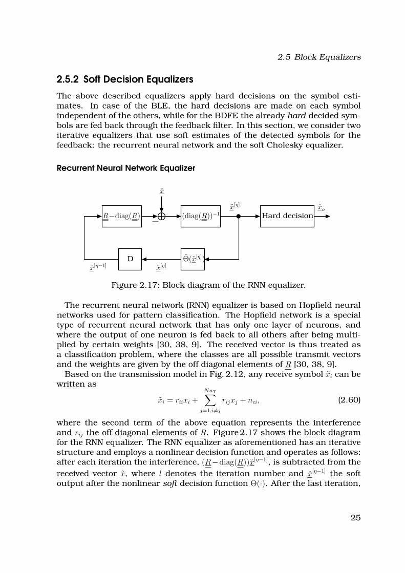
Figure 2.17: Block diagram of the RNN equalizer.
The recurrent neural network (RNN) equalizer is based on Hopfield neuralnetworks used for pattern classification. The Hopfield network is a specialtype of recurrent neural network that has only one layer of neurons, andwhere the output of one neuron is fed back to all others after being multi-plied by certain weights [30, 38, 9]. The received vector is thus treated asa classification problem, where the classes are all possible transmit vectorsand the weights are given by the off diagonal elements of R [30, 38, 9].
Based on the transmission model in Fig. 2.12, any receive symbol xi can bewritten as
xi = riixi +
NnT∑
j=1,i6=j
rijxj + nci, (2.60)
where the second term of the above equation represents the interferenceand rij the off diagonal elements of R. Figure 2.17 shows the block diagramfor the RNN equalizer. The RNN equalizer as aforementioned has an iterativestructure and employs a nonlinear decision function and operates as follows:after each iteration the interference, (R−diag(R))x[η−1], is subtracted from the
received vector x, where l denotes the iteration number and x[η−1] the softoutput after the nonlinear soft decision function Θ(·). After the last iteration,
25
2 Theoretical Background
−6 −4 −2 0 2 4 6−1
−0.5
0
0.5
1
xR
ℜ{Θ
opt(x
)}
σ2
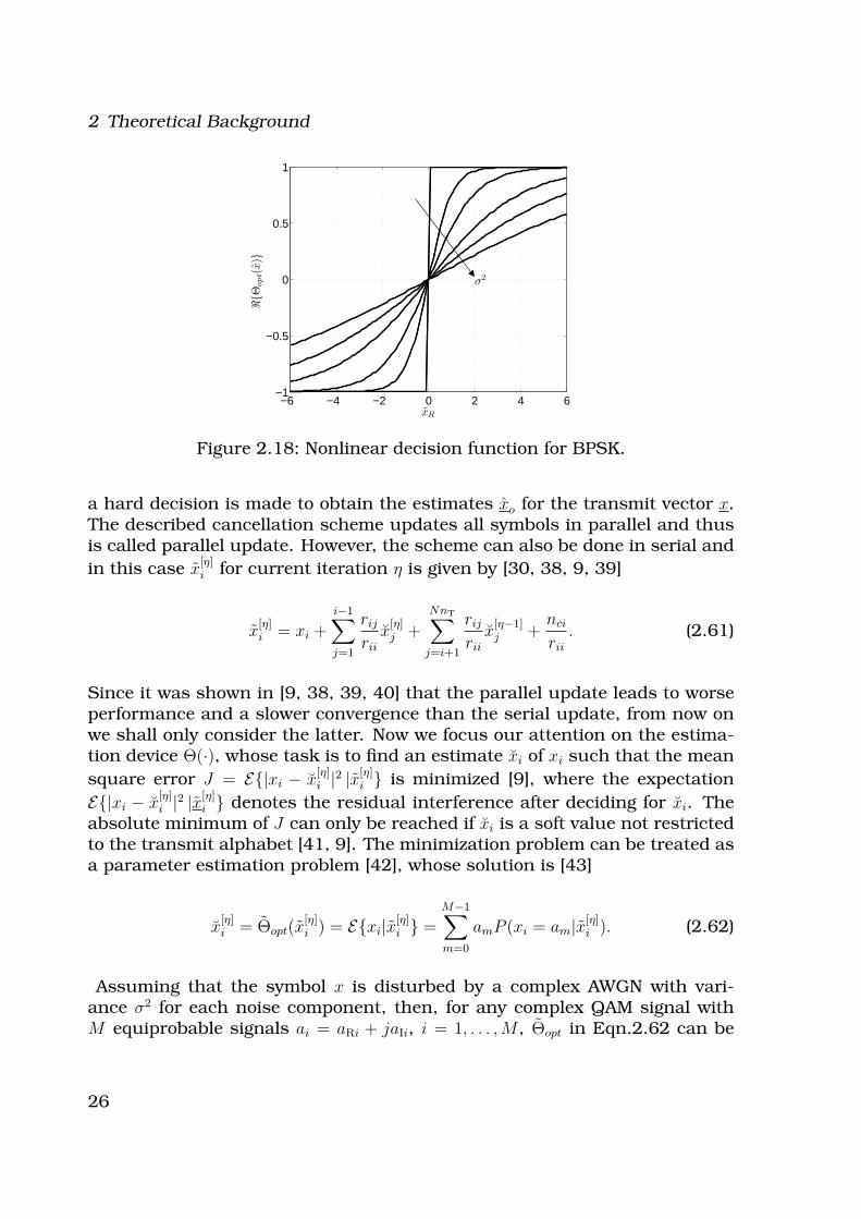
Figure 2.18: Nonlinear decision function for BPSK.
a hard decision is made to obtain the estimates xo for the transmit vector x.The described cancellation scheme updates all symbols in parallel and thusis called parallel update. However, the scheme can also be done in serial and
in this case x[η]i for current iteration η is given by [30, 38, 9, 39]
x[η]i = xi +
i−1∑
j=1
rij
rii
x[η]j +
NnT∑
j=i+1
rij
rii
x[η−1]j +
nci
rii
. (2.61)
Since it was shown in [9, 38, 39, 40] that the parallel update leads to worseperformance and a slower convergence than the serial update, from now onwe shall only consider the latter. Now we focus our attention on the estima-tion device Θ(·), whose task is to find an estimate xi of xi such that the mean
square error J = E{|xi − x[η]i |2 |x[η]
i } is minimized [9], where the expectation
E{|xi − x[η]i |2 |x[η]
i } denotes the residual interference after deciding for xi. Theabsolute minimum of J can only be reached if xi is a soft value not restrictedto the transmit alphabet [41, 9]. The minimization problem can be treated asa parameter estimation problem [42], whose solution is [43]
x[η]i = Θopt(x
[η]i ) = E{xi|x[η]
i } =M−1∑
m=0
amP (xi = am|x[η]i ). (2.62)
Assuming that the symbol x is disturbed by a complex AWGN with vari-ance σ2 for each noise component, then, for any complex QAM signal withM equiprobable signals ai = aRi + jaIi, i = 1, . . . ,M , Θopt in Eqn.2.62 can be
26
2.5 Block Equalizers
written as follows [9, 38, 40]
x = Θopt(x) =
∑Mi=1 ai exp
(
−|ai|2
2σ2 + ℜ{ai}ℜ{x}σ2 + ℑ{ai}ℑ{x}
σ2
)
∑Mi=1 exp
(
−|ai|2
2σ2 + ℜ{ai}ℜ{x}σ2 + ℑ{ai}ℑ{x}
σ2
) . (2.63)
For the special case of BPSK, Eqn. 2.63 simplifies to ℜ{Θopt(x)} = tanh(xR/σ2)and ℑ{Θopt(x)} = 0. The nonlinear decision function for increasing values ofσ2 and BPSK is shown in Fig. 2.18. As can be seen, the decision functionbecomes harder as σ2 decreases.
In order to calculate x, the noise variance, σ2, should be known. The noiseis assumed to be a sum of two statistically independent random variables:the colored noise of the channel, σ2
n,i = σ2n/|rii|2, and the residual interference
power which is assumed to be a kind of additive noise with variance σ2I,i
[η]
given as follows [9, 38]
σ2I,i
[η]=
i−1∑
j=1
|rij|2|rii|2
σ[η]res,j +
NnT∑
j=i+1
|rij|2|rii|2
σ[η−1]res,j . (2.64)
It is clear from the previous equation that σ2I,i
[η]is dependent on the iteration
number since the residual interference after each iteration is dependent on
the quality of the estimate of x. The individual interference powers σ[η]res,j are
given by [9, 38]
σ[η]res,j = E{|xj|2 |x[η]
j } − |x[η]j |2 =
∑Mi=1 |ai|2 exp
(
−|ai|2
2σ2 + ℜ{ai}ℜ{x}σ2 + ℑ{ai}ℑ{x}
σ2
)
∑Mi=1 exp
(
−|ai|2
2σ2 + ℜ{ai}ℜ{x}σ2 + ℑ{ai}ℑ{x}
σ2
) − |x[η]j |2,
(2.65)
where σ2 = σ2n,i+σ2
I,i[η]
, since the two random variables are assumed to be inde-
pendent. In case of MPSK modulation, Eqn. 2.65 reduces to σ[η]res,j = 1 − |x[η]
j |2.Clearly, the noise variance decreases with increasing number of iterations(i. e. harder decisions).
Soft Cholesky Equalizer
The SCE is derived from the ZF-BDFE and employs the same filters, how-ever, like the RNN equalizer, it is iterative and employs a soft decision deviceinstead of the hard one for feedback. Like the ZF-BDFE, the feedforward fil-ter G
f= (FH)−1 (note that the normalization by (diag(F ))−1 has been dropped
here). Thus the output of the feedforward filter is given by
ζ = F x + n, (2.66)
27
2 Theoretical Background
x ζ
n
F
(a) Block diagram of the equiva-lent vector valued transmissionscheme
x(η,l)
x(η)lζ ζ(η,l)
F\l
σ2R σ2
I
decsoft
(b) Symbol update for iteration η
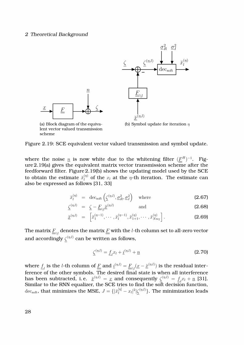
Figure 2.19: SCE equivalent vector valued transmission and symbol update.
where the noise n is now white due to the whitening filter (FH)−1. Fig-ure 2.19(a) gives the equivalent matrix vector transmission scheme after thefeedforward filter. Figure 2.19(b) shows the updating model used by the SCE
to obtain the estimate x(η)l of the xl at the η-th iteration. The estimate can
also be expressed as follows [31, 33]
x(η)l = decsoft
(
ζ(η,l), σ2R, σ2
I
)
where (2.67)
ζ(η,l) = ζ − F\lx(η,l) and (2.68)
x(η,l) =[
x(η−1)1 , · · · , x
(η−1)l , x
(η)1+1, · · · , x
(η)NnT
]
. (2.69)
The matrix F\l
denotes the matrix F with the l-th column set to all-zero vector
and accordingly ζ(η,l) can be written as follows,
ζ(η,l) = flxl + i(η,l) + n (2.70)
where flis the l-th column of F and i(η,l) = F
\l(x − x(η,l)) is the residual inter-
ference of the other symbols. The desired final state is when all interferencehas been subtracted, i. e. x(η,l) = x and consequently ζ(η,l) = f
lxl + n [31].
Similar to the RNN equalizer, the SCE tries to find the soft decision function,
decsoft, that minimizes the MSE, J = {|x[η]l − xl|2|ζ(η,l)}. The minimization leads
28
2.6 Iterative Equalization and Decoding
to the following soft decision function [31, 33]
x[η]l = E{xl|ζ(η,l)} =
M−1∑
m=0
amP (xl = am|ζ(η,l)), (2.71)
and by applying Bayes’ rule, assuming equiprobable transmit symbols andwhite disturbance we get [31, 33]
x[η]l = decsoft
(
ζ(η,l), σ2R, σ2
I
)
=M−1∑
m=0
am
[
∏NnT−1j=0 p(ζ
(η,l)j |xl = am)
∑M−1k=0
∏NnT−1j=0 p(ζ
(η,l)j |xk = am)
]
. (2.72)
Moreover, by assuming Gaussian interference the probability p(ζ(η,l)j |xl = am)
is given by [31, 33]
p(ζ(η,l)j |xl = am) =
1
2πσ(η,l)Rj σ
(η,l)Ij
exp
(
−(ℜ{ζ(η,l)j − fjlam})2
2σ2Rj
(η,l)
)
exp
(
−(ℑ{ζ(η,l)j − fjlam})2
2σ2Ij
(η,l)
)
(2.73)
and σ2Rj
(η,l)and σ2
Ij(η,l)
are given by
σRj(η,l) =
√
σ2n + i2Rj
(η,l)(2.74)
σIj(η,l) =
√
σ2n + i2Ij
(η,l). (2.75)
The decision function of the SCE thus collects all of the energy of the trans-
mit symbol xl spread over ζ(η,l)j by making the decision function dependent on
the whole column fl. Accordingly, it does not suffer from the SNR-loss that
is unavoidable for the BDFE, which can only make use of the energy on themain diagonal of F [31]. We also would like to mention at this point, thatthe difference between the RNN detector and the SCE lies in the soft deci-sion function and an additional preprocessing step of the SCE (feedforwardwhitening filter). The soft decision function of the RNN detector processes asingle symbol, whereas the SCE as aforementioned makes a decision basedon the whole symbol vector. Furthermore, since the SCE applies a whiten-ing filter, it usually offers better performance. However, the computationalcomplexity of the SCE is higher compared to that of the RNN detector.
2.6 Iterative Equalization and Decoding
In the coded case, we apply iterative equalization and decoding (also knownas turbo detection or iterative detection). Figure 2.20 depicts the discrete-time
29
2 Theoretical Background
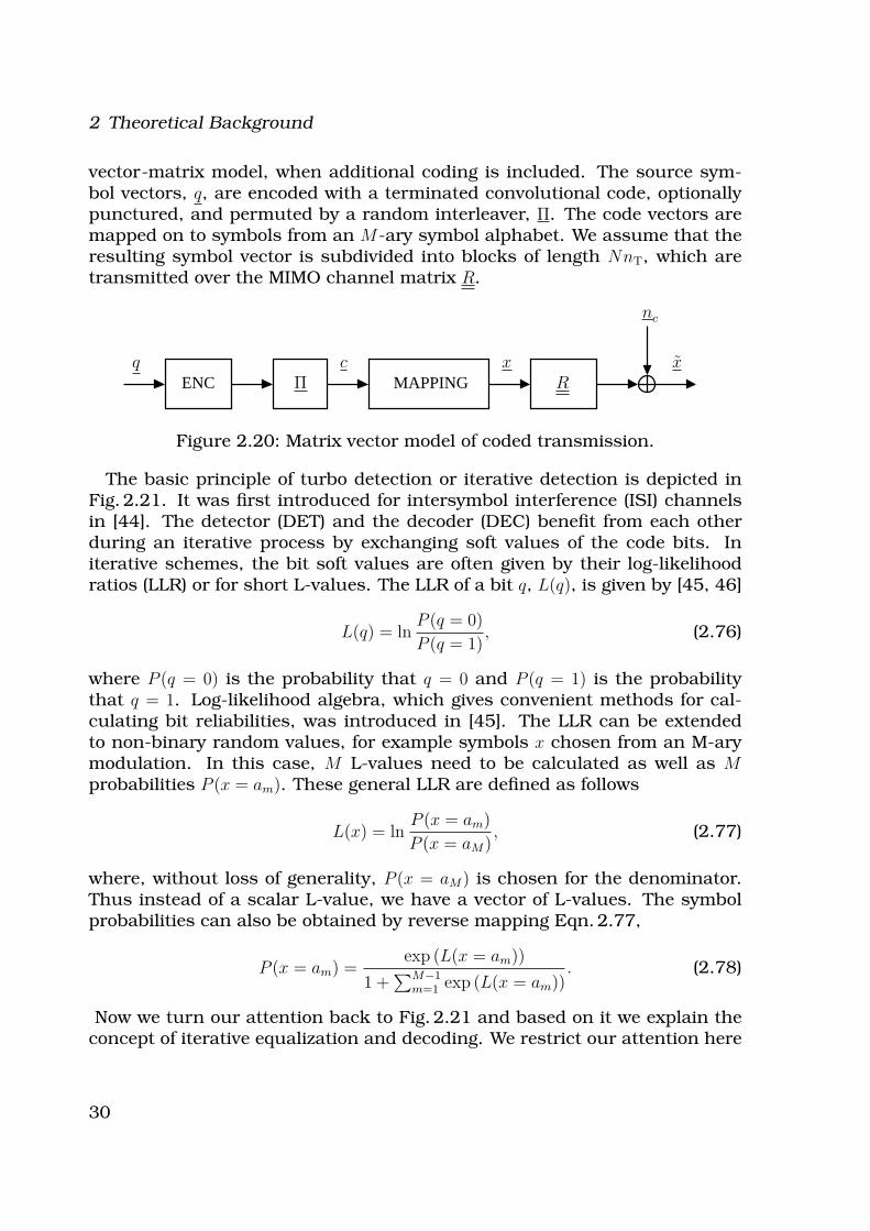
vector-matrix model, when additional coding is included. The source sym-bol vectors, q, are encoded with a terminated convolutional code, optionallypunctured, and permuted by a random interleaver, Π. The code vectors aremapped on to symbols from an M-ary symbol alphabet. We assume that theresulting symbol vector is subdivided into blocks of length NnT, which aretransmitted over the MIMO channel matrix R.
ENC MAPPINGΠq c
nc
x xR
Figure 2.20: Matrix vector model of coded transmission.
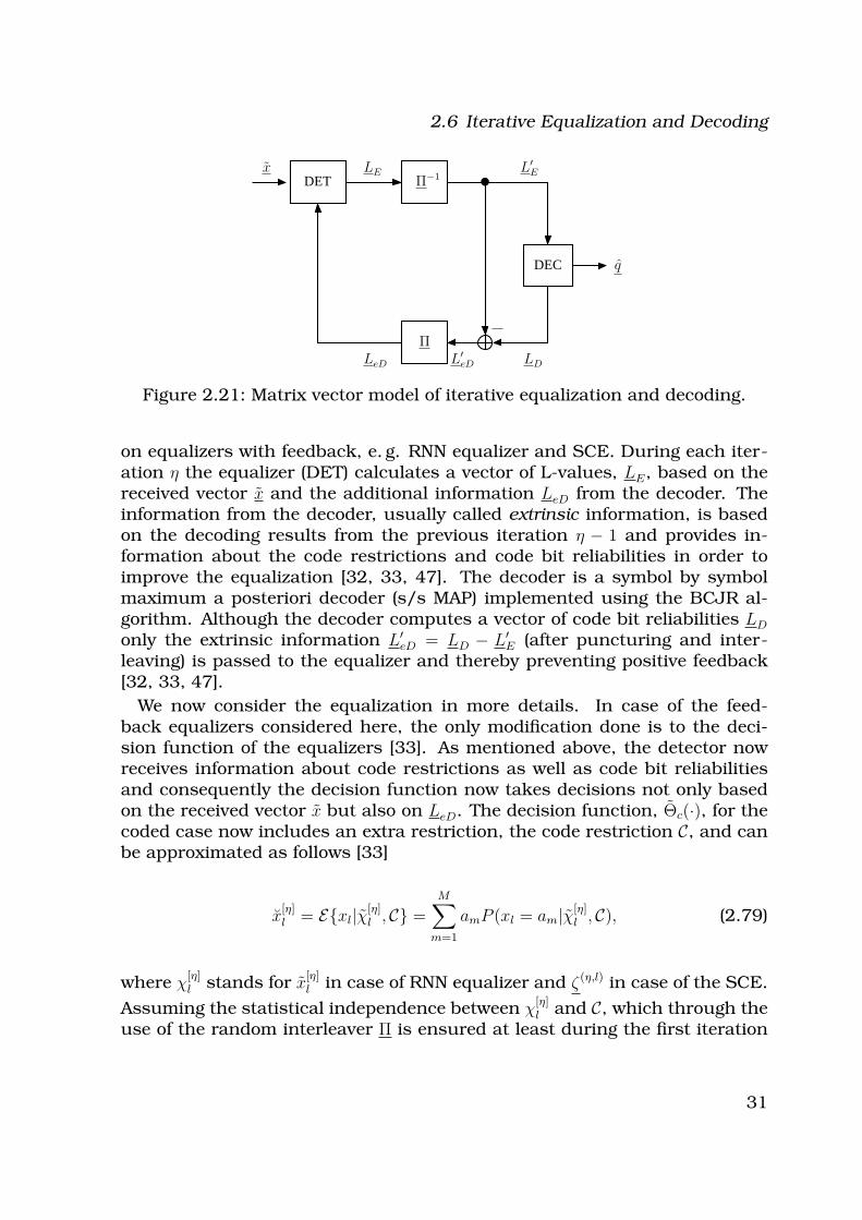
The basic principle of turbo detection or iterative detection is depicted inFig. 2.21. It was first introduced for intersymbol interference (ISI) channelsin [44]. The detector (DET) and the decoder (DEC) benefit from each otherduring an iterative process by exchanging soft values of the code bits. Initerative schemes, the bit soft values are often given by their log-likelihoodratios (LLR) or for short L-values. The LLR of a bit q, L(q), is given by [45, 46]
L(q) = lnP (q = 0)
P (q = 1), (2.76)
where P (q = 0) is the probability that q = 0 and P (q = 1) is the probabilitythat q = 1. Log-likelihood algebra, which gives convenient methods for cal-culating bit reliabilities, was introduced in [45]. The LLR can be extendedto non-binary random values, for example symbols x chosen from an M-arymodulation. In this case, M L-values need to be calculated as well as Mprobabilities P (x = am). These general LLR are defined as follows
L(x) = lnP (x = am)
P (x = aM), (2.77)
where, without loss of generality, P (x = aM) is chosen for the denominator.Thus instead of a scalar L-value, we have a vector of L-values. The symbolprobabilities can also be obtained by reverse mapping Eqn. 2.77,
P (x = am) =exp (L(x = am))
1 +∑M−1
m=1 exp (L(x = am)). (2.78)
Now we turn our attention back to Fig. 2.21 and based on it we explain theconcept of iterative equalization and decoding. We restrict our attention here
30
2.6 Iterative Equalization and Decoding
DEC
DET .
Π
Π−1
q
LE
LD
L′E
LeD L′eD
x
Figure 2.21: Matrix vector model of iterative equalization and decoding.
on equalizers with feedback, e. g. RNN equalizer and SCE. During each iter-ation η the equalizer (DET) calculates a vector of L-values, LE, based on thereceived vector x and the additional information LeD from the decoder. Theinformation from the decoder, usually called extrinsic information, is basedon the decoding results from the previous iteration η − 1 and provides in-formation about the code restrictions and code bit reliabilities in order toimprove the equalization [32, 33, 47]. The decoder is a symbol by symbolmaximum a posteriori decoder (s/s MAP) implemented using the BCJR al-gorithm. Although the decoder computes a vector of code bit reliabilities LD
only the extrinsic information L′eD = LD − L′
E (after puncturing and inter-leaving) is passed to the equalizer and thereby preventing positive feedback[32, 33, 47].
We now consider the equalization in more details. In case of the feed-back equalizers considered here, the only modification done is to the deci-sion function of the equalizers [33]. As mentioned above, the detector nowreceives information about code restrictions as well as code bit reliabilitiesand consequently the decision function now takes decisions not only basedon the received vector x but also on LeD. The decision function, Θc(·), for thecoded case now includes an extra restriction, the code restriction C, and canbe approximated as follows [33]
x[η]l = E{xl|χ[η]
l , C} =M∑
m=1
amP (xl = am|χ[η]l , C), (2.79)
where χ[η]l stands for x
[η]l in case of RNN equalizer and ζ(η,l) in case of the SCE.
Assuming the statistical independence between χ[η]l and C, which through the
use of the random interleaver Π is ensured at least during the first iteration
31
2 Theoretical Background
[32, 48], and applying Bayes’ rule we get
P (xl = am|χ[η]l , C) =
p(χ[η]l |xl = am)P (xl = am|C)
p(χ[η]l |C)
=p(χ
[η]l |xl = am)P (xl = am|C)
p(χ[η]l )
.
(2.80)The probabilities P (xl = am|C) can be represented as a function of the decoderextrinsic values LeD(cl,ν |C) [32, 48, 49],
P (xl = am|C) =
log2 M∏
ν=1
exp ((1 − bin[am, ν])LeD(cl,ν |C))
1 + exp ((LeD(cl,ν |C)), (2.81)
where bin[am, ν] denotes the value of the ν-th bit of symbol am. The channelreliability values of the code bits cl,ν, LE(cl,ν)
LE(χ[η]l |ci,ν) = ln
∑
am∈A[0]ν
p(χ[η]l |xi = am)
∑
am∈A[1]ν
p(χ[η]l |xi = am)
, (2.82)
where A[b]ν denotes the set of modulation symbols defined by a bit sequence
b at the ν-th position, and b = 0, 1. The output of the detector, LE, is thendeinterleaved Π−1 and depunctured and fed to the decoder.
Extrinsic Information Transfer Chart
The extrinsic information transfer chart or for short the EXIT chart is oneof the most well known methods for visualizing the convergence behavior ofiterative detection schemes. It is done by observing the exchange of mutualinformation between the partaking devices and was introduced by ten Brinkin [50, 51, 52]. The mutual information between two random variables X andΞ is given by [53, 54]
I(X, Ξ) =
∫
X
∫
Ξ
p(ξ, x) log2
(
p(ξ, x)
p(ξ)p(x)
)
dξdx =
∫
X
∫
Ξ
p(ξ|x)p(x) log2
(
p(ξ|x)
p(ξ)
)
dξdx,
(2.83)where we made use of the relation p(ξ, x) = p(ξ|x)p(x) to obtain the right-hand side of the above equation. We first consider the decoder and assume
perfect interleaving i. e. we assume the input L-values, LE(χ[η]l |ci,ν), to be
independent and identically distributed random variables AD. The probabilitydensity function (pdf) of AD conditioned on the code bits p(ζ|c) is Gaussianwith mean σ2
A and mean σ2A/2(1 − 2b), where b = 0, 1 [51, 52],
pAD(ζ|c = b) =
1√
2πσ2A
exp
(
−ζ − σ2A
2b
2σ2A
)
. (2.84)
32
2.6 Iterative Equalization and Decoding
Thus, the mutual information, IA,dec, between the input L-values AD and theunmapped code bits according to Eqn. 2.83, assuming equiprobable codebits, is [51, 52]
IA,dec =1
2
∑
b=−1,1
∫ ∞
−∞
pAD(ζ|c = b) log2
(
2pAD(ζ|c = b)
pAD(ζ|c = −1) + pAD
(ζ|c = 1)
)
dξ. (2.85)
The pdf of the extrinsic output L-values of the decoder, LeD(ci,ν |C), condi-tioned on the code bits, pED
(ζ|c = b), can not be calculated and are measuredusing Monte Carlo simulations. The mutual information at the output of thedecoder, IE,dec, between the code bits c and the random output L-values ED
are then calculated as in Eqn. 2.85. Since IA,dec is monotonically increasingin σ2
A and thus invertible, artificial L-values with mean σ2A/2(1 − 2b), and
variance σ2A can be generated for a given value of IA,dec. The generated
L-values are then fed to the decoder and pED(ζ|c = b) of ED and in turn IE,dec
are calculated.
The extrinsic information for the SCE and the RNN equalizer can not beobtained by the previously described straightforward method. The abovederivation of the EXIT-chart assumes memory-less components, a conditionthat does not apply to feedback equalizers such as the SCE and RNN.These equalizers use decisions from previous iterations for interferencecancellation and thus have memory. However, the condition of memory-lesscomponents can be relaxed so as to be able to find EXIT charts for the SCEand RNN [33]. This can be achieved by running those equalizers for severaliterations using the same extrinsic information for all iterations and therebyreducing the memory effect [33, 35, 48]. In other words, extrinsic L-valuesof the decoder are artificially generated and fed to the equalizer which isthen allowed to run for more than one iteration while keeping the L-valuesunaltered. As the number of iterations tends to infinity, an upperboundfor the extrinsic transfer characteristics of the feedback equalizers can beobtained. Yet, it was shown in [33, 35, 48] that the extrinsic transfer curvesfor more than one iteration lie very close to each other. The curves for two orthree iterations are thus enough to approximate the extrinsic transfer curvesof the feedback equalizers.
Now, to analyze the convergence behavior of iterative equalization and de-coding, the EXIT charts for both the equalizer and decoder are included inthe same graph, where the input to the decoder is equal to the output ofthe equalizer (IA,dec = IE,eq on the ordinate) and the output of the decoder isequal to the input of the equalizer (IE,dec = IA,eq on the abscissa). Note thatthe decoder chart is now flipped. A schematic of the EXIT charts for the
33
2 Theoretical Background
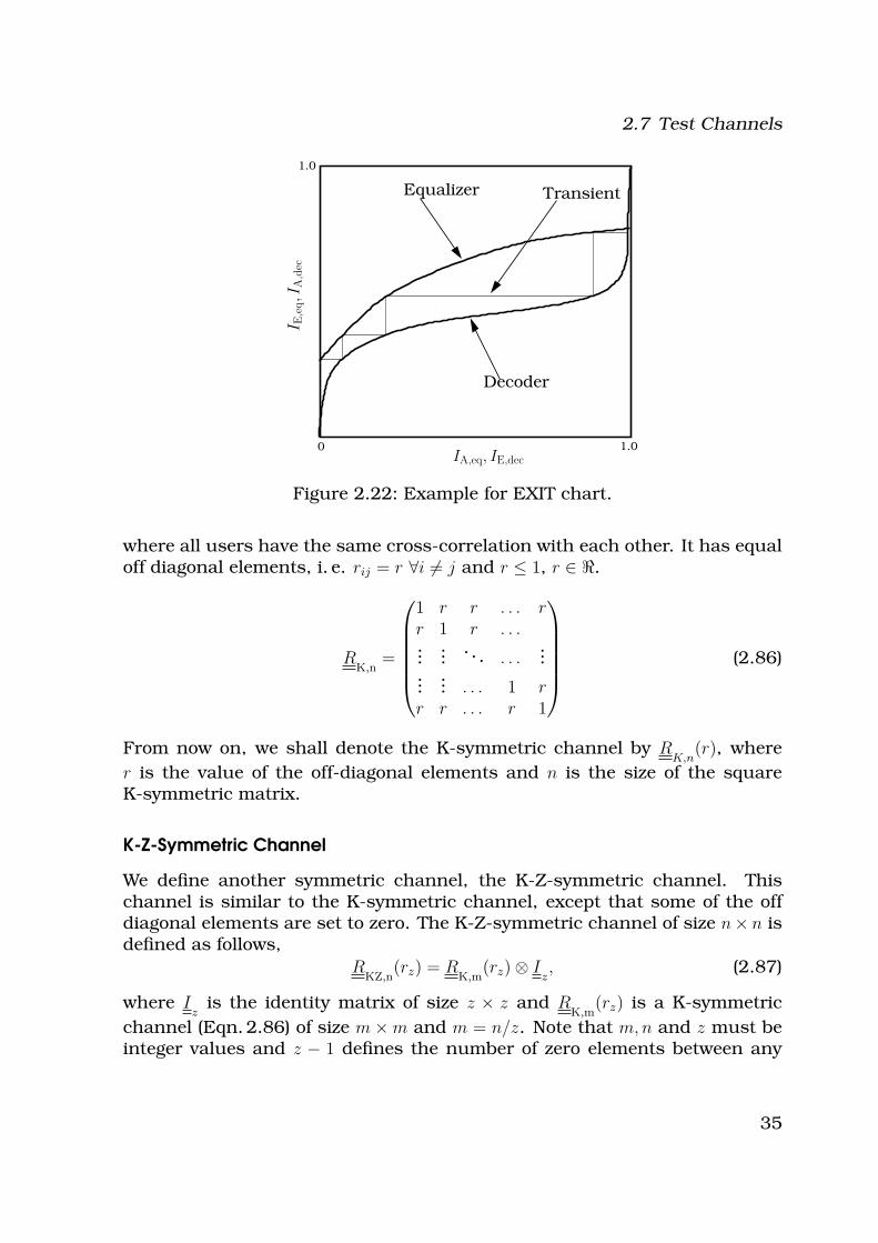
equalizer and decoder is shown Fig. 2.22. The iterative process starts withthe equalizer and ends with the decoder. The starting point is thus IE,eq forIA,eq = 0 i. e. no extrinsic information available. After that, the equalizer out-put becomes the decoder input i. e. IA,dec = IE,eq. This is represented by a lineparallel to the abscissa starting at the previous IE,eq point and ending at theintersection with the decoder chart at some new IE,dec. This is the decoderoutput which in turn becomes the equalizer input IE,dec = IA,eq. Similarly, thisis represented by a line parallel to the ordinate starting at the previous IE,dec
and ending at the intersection with the equalizer chart at a new point IE,eq.This is continued until equalizer and decoder EXIT characteristics intersect.This intersection point is important since the hard decision are made afterthe decoder in the last iteration i. e. a higher IE,dec corresponds to lower BER.Those above described lines are called the transient trajectory and, as can beseen in Fig. 2.22, they are upper bounded by the equalizer EXIT characteris-tics and lower bounded by the decoder EXIT characteristics. The convergencespeed of the iterative process is thus dependent on the size and shape of theenclosed area. The larger the enclosed area the faster the convergence i. e.less iterations are required to achieve the best performance. It was shownthrough simulation results in [33, 18, 48, 19] that the starting point IE,eq ofthe equalizer chart is highly dependent on the amount of interference in thechannel, where higher interference leads to lower IE,eq values. The final IE,eq
on the other hand was found to be dependent on the matched filter bound(MFB), with better MFB leading to higher final IE,eq values. We shall look atthis behavior again in more details in Chapter 4. It is also important to men-tion at this point, that those transient trajectories should only be seen asan approximation and that the actual trajectory may be significantly differ-ent from the above described theoretical trajectory. For example, the actualtrajectory does not have to hit either of the EXIT characteristic curves.
2.7 Test Channels
To assess the effect of the total interference and the distribution of the in-dividual interference values as well as the MFB on the performance of theequalizers described in Sec. 2.5, two standard channels are proposed in thissection. These channels are then used for judging the behavior of the equal-izers under different interference and matched filter bound (MFB) conditions.
K-Symmetric Channel
The K-symmetric channel is an n×n correlation matrix and was first definedin [55]. It was used to describe the cross-correlation matrix between K users,
34
2.7 Test Channels
PSfrag
IA,eq, IE,dec
I E,e
q,I
A,d
ec
Transient
Decoder
Equalizer
0 1.0
1.0
Figure 2.22: Example for EXIT chart.
where all users have the same cross-correlation with each other. It has equaloff diagonal elements, i. e. rij = r ∀i 6= j and r ≤ 1, r ∈ ℜ.
RK,n
=
1 r r . . . rr 1 r . . ....
.... . . . . .
......
... . . . 1 rr r . . . r 1
(2.86)
From now on, we shall denote the K-symmetric channel by RK,n
(r), where
r is the value of the off-diagonal elements and n is the size of the squareK-symmetric matrix.
K-Z-Symmetric Channel
We define another symmetric channel, the K-Z-symmetric channel. Thischannel is similar to the K-symmetric channel, except that some of the offdiagonal elements are set to zero. The K-Z-symmetric channel of size n× n isdefined as follows,
RKZ,n
(rz) = RK,m
(rz) ⊗ Iz, (2.87)
where Iz
is the identity matrix of size z × z and RK,m
(rz) is a K-symmetric
channel (Eqn. 2.86) of size m × m and m = n/z. Note that m,n and z must beinteger values and z − 1 defines the number of zero elements between any
35
2 Theoretical Background
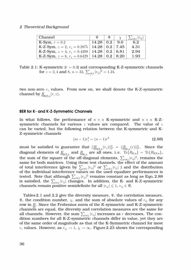
Channel Ψ Φ χ∑
i6=j |rij|K-Sym, r = 0.2 14.28 0.2 9.0 6.2K-Z-Sym, z = 2, rz = 0.2875 14.28 0.2 7.45 4.31K-Z-Sym, z = 4, rz = 0.4209 14.28 0.2 6.81 2.94K-Z-Sym, z = 8, rz = 0.6429 14.28 0.2 8.20 1.93
Table 2.1: K-symmetric (r = 0.3) and corresponding K-Z-symmetric channelsfor z = 2, 4 and 8, n = 32,
∑
i6=j |rij|2 = 1.24..
two non-zero rz values. From now on, we shall denote the K-Z-symmetricchannel by R
KZ,n(r, z).
BER for K- and K-Z-Symmetric Channels
In what follows, the performance of n × n K-symmetric and n × n K-Z-symmetric channels for various z values are compared. The value of zcan be varied, but the following relation between the K-symmetric and K-Z-symmetric channels
(m − 1)r2z = (n − 1)r2 (2.88)
must be satisfied to guarantee that ||RKZ,n
(rz)||2F = ||RK,n
(r)||2F . Since the
diagonal elements of RKZ,n
and RK,n
are all ones, i. e. Tr{RK,n} = Tr{RKZ,n},the sum of the square of the off-diagonal elements,
∑
i6=j |rij|2, remains thesame for both matrices. Using these test channels, the effect of the amountof total interference (given by
∑
i6=j |rij|2 or∑
i6=j |rij| ) and the distributionof the individual interference values on the used equalizer performances istested. Note that although
∑
i6=j |rij|2 remains constant as long as Eqn. 2.88is satisfied, the
∑
i6=j |rij| changes. In addition, the K- and K-Z-symmetricchannels remain positive semidefinite for all |rij| ≤ 1, rij ∈ ℜ.
Tables 2.1 and 2.2 give the diversity measure, Ψ, the correlation measure,Φ, the condition number, χ, and the sum of absolute values of rij for anyrow in R. Since the Frobenius norm of the K-symmetric and K-Z-symmetricchannels are equal, the diversity and correlation measures are the same forall channels. However, the sum
∑
i6=j |rij| increases as r decreases. The con-dition numbers for all K-Z-symmetric channels differ in value, yet they areof the same order of magnitude as that of the K-Symmetric channel for mostrz values. However, as rij → 1, χ → ∞. Figure 2.23 shows the corresponding
36
2.7 Test Channels
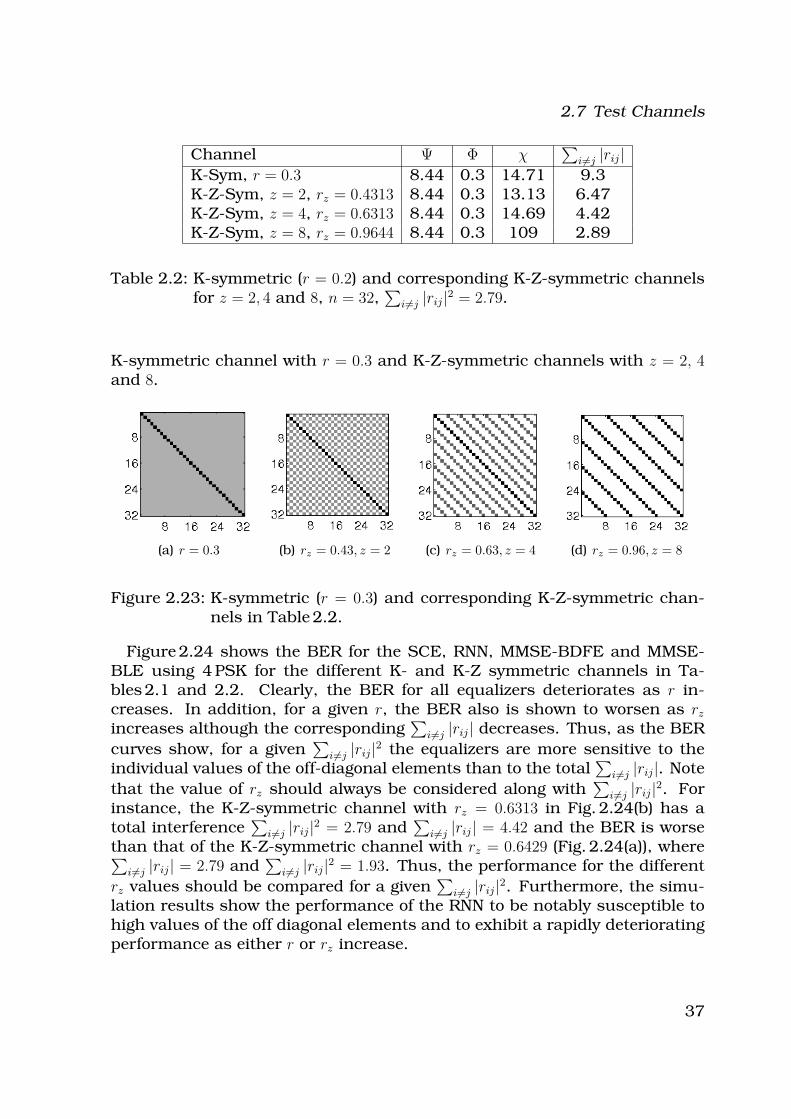
Channel Ψ Φ χ∑
i6=j |rij|K-Sym, r = 0.3 8.44 0.3 14.71 9.3K-Z-Sym, z = 2, rz = 0.4313 8.44 0.3 13.13 6.47K-Z-Sym, z = 4, rz = 0.6313 8.44 0.3 14.69 4.42K-Z-Sym, z = 8, rz = 0.9644 8.44 0.3 109 2.89
Table 2.2: K-symmetric (r = 0.2) and corresponding K-Z-symmetric channelsfor z = 2, 4 and 8, n = 32,
∑
i6=j |rij|2 = 2.79.
K-symmetric channel with r = 0.3 and K-Z-symmetric channels with z = 2, 4and 8.
(a) r = 0.3 (b) rz = 0.43, z = 2 (c) rz = 0.63, z = 4 (d) rz = 0.96, z = 8
Figure 2.23: K-symmetric (r = 0.3) and corresponding K-Z-symmetric chan-nels in Table 2.2.
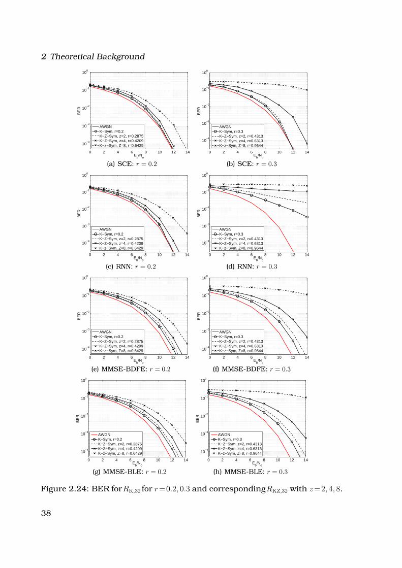
Figure 2.24 shows the BER for the SCE, RNN, MMSE-BDFE and MMSE-BLE using 4 PSK for the different K- and K-Z symmetric channels in Ta-bles 2.1 and 2.2. Clearly, the BER for all equalizers deteriorates as r in-creases. In addition, for a given r, the BER also is shown to worsen as rz
increases although the corresponding∑
i6=j |rij| decreases. Thus, as the BER
curves show, for a given∑
i6=j |rij|2 the equalizers are more sensitive to theindividual values of the off-diagonal elements than to the total
∑
i6=j |rij|. Note
that the value of rz should always be considered along with∑
i6=j |rij|2. Forinstance, the K-Z-symmetric channel with rz = 0.6313 in Fig. 2.24(b) has atotal interference
∑
i6=j |rij|2 = 2.79 and∑
i6=j |rij| = 4.42 and the BER is worsethan that of the K-Z-symmetric channel with rz = 0.6429 (Fig. 2.24(a)), where∑
i6=j |rij| = 2.79 and∑
i6=j |rij|2 = 1.93. Thus, the performance for the different
rz values should be compared for a given∑
i6=j |rij|2. Furthermore, the simu-lation results show the performance of the RNN to be notably susceptible tohigh values of the off diagonal elements and to exhibit a rapidly deterioratingperformance as either r or rz increase.
37
2 Theoretical Background
0 2 4 6 8 10 12 14
10−4
10−3
10−2
10−1
100
Eb/N
o
BE
R
AWGNK−Sym, r=0.2K−Z−Sym, z=2, r=0.2875K−Z−Sym, z=4, r=0.4209K−z−Sym, Z=8, r=0.6429
(a) SCE: r = 0.2
0 2 4 6 8 10 12 14
10−4
10−3
10−2
10−1
100
Eb/N
o
BE
R
AWGNK−Sym, r=0.3K−Z−Sym, z=2, r=0.4313K−Z−Sym, z=4, r=0.6313K−z−Sym, Z=8, r=0.9644
(b) SCE: r = 0.3
0 2 4 6 8 10 12 14
10−4
10−3
10−2
10−1
100
Eb/N
o
BE
R
AWGNK−Sym, r=0.2K−Z−Sym, z=2, r=0.2875K−Z−Sym, z=4, r=0.4209K−z−Sym, Z=8, r=0.6429
(c) RNN: r = 0.2
0 2 4 6 8 10 12 14
10−4
10−3
10−2
10−1
100
Eb/N
o
BE
R
AWGNK−Sym, r=0.3K−Z−Sym, z=2, r=0.4313K−Z−Sym, z=4, r=0.6313K−z−Sym, Z=8, r=0.9644
(d) RNN: r = 0.3
0 2 4 6 8 10 12 14
10−4
10−3
10−2
10−1
100
Eb/N
o
BE
R
AWGNK−Sym, r=0.2K−Z−Sym, z=2, r=0.2875K−Z−Sym, z=4, r=0.4209K−z−Sym, Z=8, r=0.6429
(e) MMSE-BDFE: r = 0.2
0 2 4 6 8 10 12 14
10−4
10−3
10−2
10−1
100
Eb/N
o
BE
R
AWGNK−Sym, r=0.3K−Z−Sym, z=2, r=0.4313K−Z−Sym, z=4, r=0.6313K−z−Sym, Z=8, r=0.9644
(f) MMSE-BDFE: r = 0.3
0 2 4 6 8 10 12 14
10−4
10−3
10−2
10−1
100
Eb/N
o
BE
R
AWGNK−Sym, r=0.2K−Z−Sym, z=2, r=0.2875K−Z−Sym, z=4, r=0.4209K−z−Sym, Z=8, r=0.6429
(g) MMSE-BLE: r = 0.2
0 2 4 6 8 10 12 14
10−4
10−3
10−2
10−1
100
Eb/N
o
BE
R
AWGNK−Sym, r=0.3K−Z−Sym, z=2, r=0.4313K−Z−Sym, z=4, r=0.6313K−z−Sym, Z=8, r=0.9644
(h) MMSE-BLE: r = 0.3
Figure 2.24: BER forRK,32 for r=0.2, 0.3 and correspondingRKZ,32 with z=2, 4, 8.
38
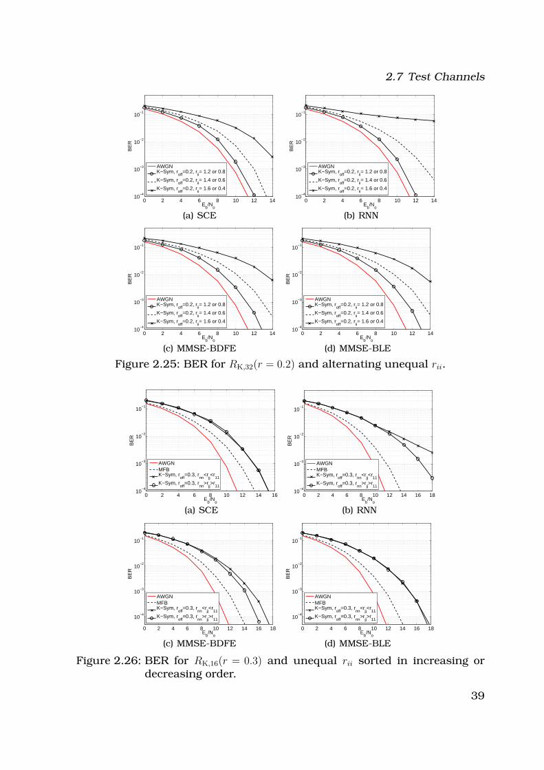
2.7 Test Channels
0 2 4 6 8 10 12 1410
−4
10−3
10−2
10−1
Eb/N
o
BE
R
AWGNK−Sym, r
off=0.2, r
ii= 1.2 or 0.8
K−Sym, roff
=0.2, rii= 1.4 or 0.6
K−Sym, roff
=0.2, rii= 1.6 or 0.4
(a) SCE
0 2 4 6 8 10 12 1410
−4
10−3
10−2
10−1
Eb/N
o
BE
R
AWGNK−Sym, r
off=0.2, r
ii= 1.2 or 0.8
K−Sym, roff
=0.2, rii= 1.4 or 0.6
K−Sym, roff
=0.2, rii= 1.6 or 0.4
(b) RNN
0 2 4 6 8 10 12 1410
−4
10−3
10−2
10−1
Eb/N
o
BE
R
AWGNK−Sym, r
off=0.2, r
ii= 1.2 or 0.8
K−Sym, roff
=0.2, rii= 1.4 or 0.6
K−Sym, roff
=0.2, rii= 1.6 or 0.4
(c) MMSE-BDFE
0 2 4 6 8 10 12 1410
−4
10−3
10−2
10−1
Eb/N
o
BE
R
AWGNK−Sym, r
off=0.2, r
ii= 1.2 or 0.8
K−Sym, roff
=0.2, rii= 1.4 or 0.6
K−Sym, roff
=0.2, rii= 1.6 or 0.4
(d) MMSE-BLE
Figure 2.25: BER for RK,32(r = 0.2) and alternating unequal rii.
0 2 4 6 8 10 12 14 1610
−4
10−3
10−2
10−1
Eb/N
o
BE
R
AWGNMFBK−Sym, r
off=0.3, r
nn<r
jj<r
11K−Sym, r
off=0.3, r
nn>r
jj>r
11
(a) SCE
0 2 4 6 8 10 12 14 16 1810
−4
10−3
10−2
10−1
Eb/N
o
BE
R
AWGNMFBK−Sym, r
off=0.3, r
nn<r
jj<r
11K−Sym, r
off=0.3, r
nn>r
jj>r
11
(b) RNN
0 2 4 6 8 10 12 14 16 18
10−4
10−3
10−2
10−1
Eb/N
o
BE
R
AWGNMFBK−Sym, r
off=0.3, r
nn<r
jj<r
11K−Sym, r
off=0.3, r
nn>r
jj>r
11
(c) MMSE-BDFE
0 2 4 6 8 10 12 14 16 18
10−4
10−3
10−2
10−1
Eb/N
o
BE
R
AWGNMFBK−Sym, r
off=0.3, r
nn<r
jj<r
11K−Sym, r
off=0.3, r
nn>r
jj>r
11
(d) MMSE-BLE
Figure 2.26: BER for RK,16(r = 0.3) and unequal rii sorted in increasing ordecreasing order.
39
2 Theoretical Background
Effect of the MFB
Here, we modify the K-symmetric and K-Z-symmetric channels, such thatthe diagonal elements are not longer equal to one. The sum of the diagonalelements remains however the same. In Fig. 2.25, the diagonal elements, rii,alternatingly take on two different values, while in Fig. 2.26 the diagonal ele-
ments are sorted either in increasing or decreasing order with rii = 0.87(1.1−l),and l = −(n/2 − 1), . . . , n/2. Note that the diagonal elements had to be care-fully chosen so that the resulting channels remain positive definite. Theoff-diagonal elements are all equal and remain the same irrespective of thevalue of the diagonal elements. This way, we can test the effect of the MFBon the BER performance of the employed equalizers. Figures 2.25 and 2.26show that the performance of all equalizers deteriorates as the MFB worsens,i. e. as the difference between the values of the diagonal elements increases.In addition, the RNN and MMSE-BDFE equalizers are sensitive to the orderof sorting (increasing or decreasing) of the diagonal elements as can be seenin Figs. 2.26(b) and 2.26(c). They both seem to be more sensitive to propaga-tion errors than the SCE. The MMSE-BLE, as expected, is not affected by theorder since it does not employ any feedback filters.
The results of the test channels give a guideline as to how the differentequalizers perform and how this performance is affected by interference, itsdistribution and MFB. They thus aid in predicting their operation for otherchannels as will be shown in the next chapters.
2.8 Summary
In this chapter, we described the matrix vector transmission model forSISO-OFDM and extended it to MIMO-OFDM systems and presented howspreading can be incorporated into that model. In addition, we showed howantenna correlations can be integrated in the MIMO-OFDM channel model.We described four different suboptimum equalizers (SCE, RNN, MMSE-BLEand MMSE-BDFE) that will be used throughout this work and presentedhow the RNN equalizer and SCE can be incorporated in iterative equalizationand decoding schemes. We have also looked at the performance of thosesuboptimal equalizers for a set of test channels and showed that the perfor-mance is dependent on the MFB as well as on the amount of interference.The performance of the equalizers for those test channels will be used asa guideline to judge their performance in MIMO frequency selective channels.
40
Chapter3Spreading
Time, frequency and spatial diversity are available for signals transmittedover frequency selective, time varying MIMO channels. In order to capturethose diversities, signals need to be coded. The codeword dimensions de-pend in general on the number of transmit and receive antennas as well asthe codeword duration and bandwidth. In addition, the maximum diver-sity that can be captured by a codeword depends on the coherence time,coherence distance and coherence bandwidth. For instance, the maximumavailable time diversity a codeword of duration T can capture is T/Tc, whereTc is the coherence time. Similarly, for a bandwidth BW and coherence band-width BWc, BW/BWc represents the number of frequency diversity branches.In addition, the MIMO antennas must be at least separated by the coher-ence distance. Intuitively speaking, diversity gain can be seen as the numberof independently fading paths that a symbol is transmitted through. In aflat fading channel with nT transmit antennas and nR receive antennas, themaximum achievable diversity is nTnR for a codeword of duration T ≤ Tc.In a frequency selective channel with L taps, the maximum achievable di-versity would be nTnRL. In this Chapter, we consider spreading techniquesfor frequency selective MIMO channels assuming no channel knowledge at
41
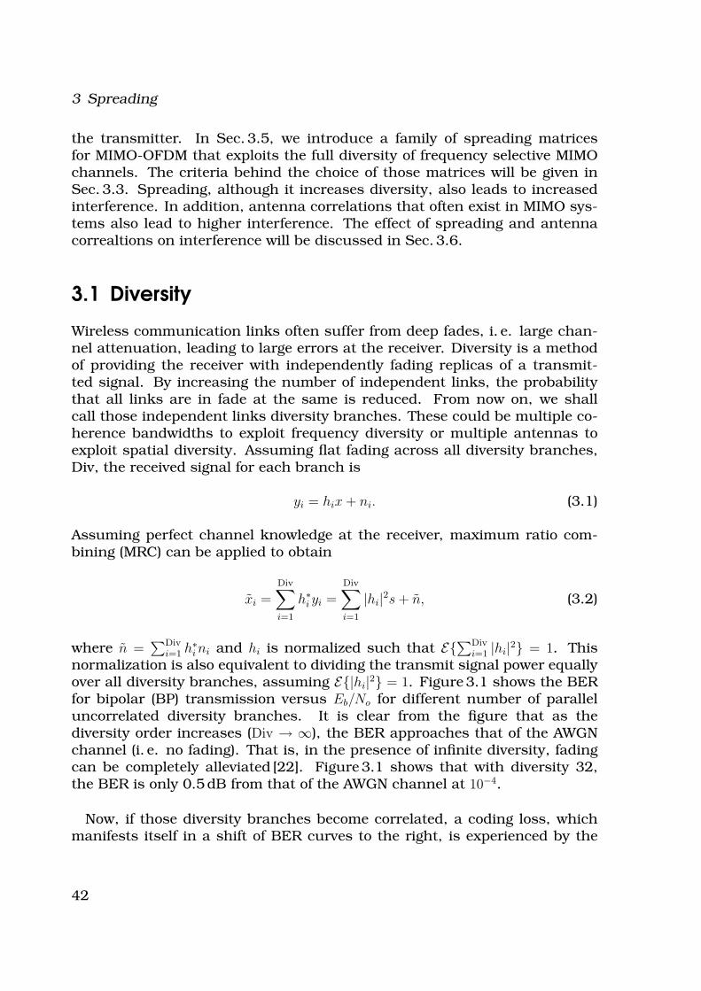
3 Spreading
the transmitter. In Sec. 3.5, we introduce a family of spreading matricesfor MIMO-OFDM that exploits the full diversity of frequency selective MIMOchannels. The criteria behind the choice of those matrices will be given inSec. 3.3. Spreading, although it increases diversity, also leads to increasedinterference. In addition, antenna correlations that often exist in MIMO sys-tems also lead to higher interference. The effect of spreading and antennacorrealtions on interference will be discussed in Sec. 3.6.
3.1 Diversity
Wireless communication links often suffer from deep fades, i. e. large chan-nel attenuation, leading to large errors at the receiver. Diversity is a methodof providing the receiver with independently fading replicas of a transmit-ted signal. By increasing the number of independent links, the probabilitythat all links are in fade at the same is reduced. From now on, we shallcall those independent links diversity branches. These could be multiple co-herence bandwidths to exploit frequency diversity or multiple antennas toexploit spatial diversity. Assuming flat fading across all diversity branches,Div, the received signal for each branch is
yi = hix + ni. (3.1)
Assuming perfect channel knowledge at the receiver, maximum ratio com-bining (MRC) can be applied to obtain
xi =Div∑
i=1
h∗i yi =
Div∑
i=1
|hi|2s + n, (3.2)
where n =∑Div
i=1 h∗i ni and hi is normalized such that E{∑Div
i=1 |hi|2} = 1. Thisnormalization is also equivalent to dividing the transmit signal power equallyover all diversity branches, assuming E{|hi|2} = 1. Figure 3.1 shows the BERfor bipolar (BP) transmission versus Eb/No for different number of paralleluncorrelated diversity branches. It is clear from the figure that as thediversity order increases (Div → ∞), the BER approaches that of the AWGNchannel (i. e. no fading). That is, in the presence of infinite diversity, fadingcan be completely alleviated [22]. Figure 3.1 shows that with diversity 32,the BER is only 0.5 dB from that of the AWGN channel at 10−4.
Now, if those diversity branches become correlated, a coding loss, whichmanifests itself in a shift of BER curves to the right, is experienced by the
42
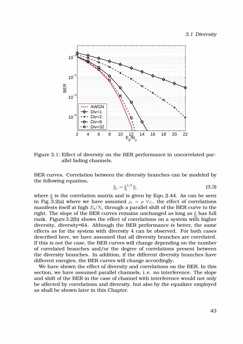
3.1 Diversity
2 4 6 8 10 12 14 16 18 20 22
10−4
10−3
10−2
10−1
Eb/N
o
BE
R
AWGNDiv=1Div=2Div=8Div=32
Figure 3.1: Effect of diversity on the BER performance in uncorrelated par-allel fading channels.
BER curves. Correlation between the diversity branches can be modeled bythe following equation,
hc = k1/2 h, (3.3)
where k is the correlation matrix and is given by Eqn. 2.44. As can be seenin Fig. 3.2(a) where we have assumed ρi = ρ ∀ i., the effect of correlationsmanifests itself at high Eb/No through a parallel shift of the BER curve to theright. The slope of the BER curves remains unchanged as long as k has fullrank. Figure 3.2(b) shows the effect of correlations on a system with higherdiversity, diversity=64. Although the BER performance is better, the sameeffects as for the system with diversity 4 can be observed. For both casesdescribed here, we have assumed that all diversity branches are correlated.If this is not the case, the BER curves will change depending on the numberof correlated branches and/or the degree of correlations present betweenthe diversity branches. In addition, if the different diversity branches havedifferent energies, the BER curves will change accordingly.
We have shown the effect of diversity and correlations on the BER. In thissection, we have assumed parallel channels, i. e. no interference. The slopeand shift of the BER in the case of channel with interference would not onlybe affected by correlations and diversity, but also by the equalizer employedas shall be shown later in this Chapter.
43
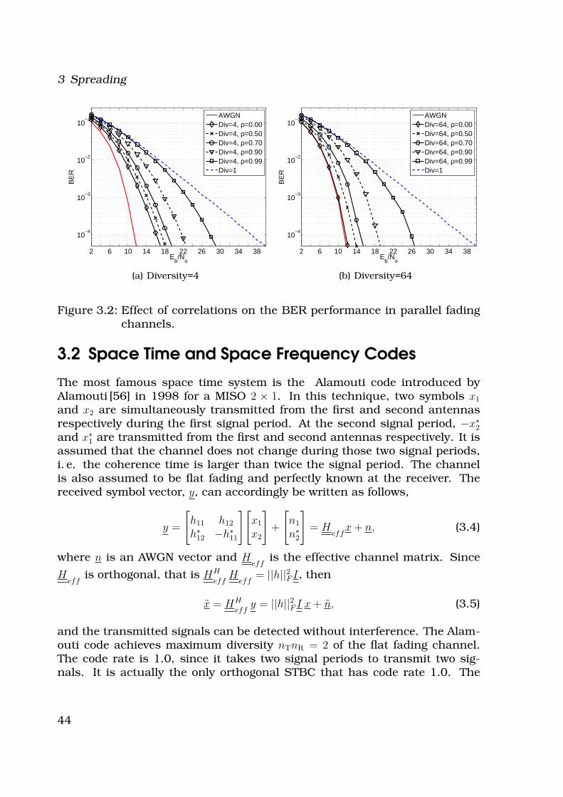
3 Spreading
2 6 10 14 18 22 26 30 34 38
10−4
10−3
10−2
10−1
Eb/N
o
BE
R
AWGNDiv=4, ρ=0.00Div=4, ρ=0.50Div=4, ρ=0.70Div=4, ρ=0.90Div=4, ρ=0.99Div=1
(a) Diversity=4
2 6 10 14 18 22 26 30 34 38
10−4
10−3
10−2
10−1
Eb/N
o
BE
R
AWGNDiv=64, ρ=0.00Div=64, ρ=0.50Div=64, ρ=0.70Div=64, ρ=0.90Div=64, ρ=0.99Div=1
(b) Diversity=64
Figure 3.2: Effect of correlations on the BER performance in parallel fadingchannels.
3.2 Space Time and Space Frequency Codes
The most famous space time system is the Alamouti code introduced byAlamouti [56] in 1998 for a MISO 2 × 1. In this technique, two symbols x1
and x2 are simultaneously transmitted from the first and second antennasrespectively during the first signal period. At the second signal period, −x∗
2
and x∗1 are transmitted from the first and second antennas respectively. It is
assumed that the channel does not change during those two signal periods,i. e. the coherence time is larger than twice the signal period. The channelis also assumed to be flat fading and perfectly known at the receiver. Thereceived symbol vector, y, can accordingly be written as follows,
y =
[
h11 h12
h∗12 −h∗
11
][
x1
x2
]
+
[
n1
n∗2
]
= Heff
x + n, (3.4)
where n is an AWGN vector and Heff
is the effective channel matrix. Since
Heff
is orthogonal, that is HH
effH
eff= ||h||2F I, then
x = HH
effy = ||h||2F I x + n, (3.5)
and the transmitted signals can be detected without interference. The Alam-outi code achieves maximum diversity nTnR = 2 of the flat fading channel.The code rate is 1.0, since it takes two signal periods to transmit two sig-nals. It is actually the only orthogonal STBC that has code rate 1.0. The
44
3.2 Space Time and Space Frequency Codes
above Alamouti scheme, although it requires only one receive antenna, canbe used with multiple receive antennas which leads to improved BER andhigher diversity. The design of STBC for larger number of transmit antennascan be found in [57]. In this work, the authors introduced two design criteriafor ST code construction: the rank criterion and the determinant criterion.These criteria are based on the pairwise error probability (PEP) between anytwo codewords assuming maximum likelihood (ML) detection. For Rayleighfading, the upperbound on the PEP between any two codewords C and Eaveraged over all channels for high SNR (Es/No >> 1) is
P (C → E) ≤ 1(
Πr(Y )
k=1 λk(Y ))nR
(
Es
4No
)−r(Y )nR
, (3.6)
where Y = G GH, G = C −E, λk(Y ) are the non-zero eigenvalues of G and r(Y )is the rank of Y (which is also equal to the rank of G). The rank criterionoptimizes the diversity gain while the determinant criterion optimizes thecoding gain. To achieve maximum diversity nTnR, the matrix G must be offull rank for any two codeword pairs. To maximize the coding gain givena diversity target of nTnR, the minimum of the determinant of Y must bemaximized for all pairs of codewords [57]. The coding gain is a measure of thegain due to coding compared to an uncoded system with the same diversity.At high SNR, the coding gain leads to a shift in the SER curve to the left whilethe diversity gain to an increase in its slope [22].
In [58], the authors showed that space-time codes designed to achieve fulldiversity in flat fading environment will in general not achieve the full space-frequency diversity, since they do not exploit the extra frequency diversityavailable. Similar to [57], they presented a design criteria for MIMO-OFDMalso based on the pairwise error probability and maximum likelihood detec-tion. The authors took the frequency diversity into account when deriving thedesign criteria. Assuming no spatial or tap correlations and a uniform powerdelay profile of the Rayleigh fading channels, the pairwise error probability,after averaging over all channel realizations, can be written as [58]
P (C → E) =
r(Y )∏
i=0
(
1 +Es
4No
λi(Y )
)−nR
. (3.7)
The matrix Y = G GH where
G = [(C − E)T D(C − E)T · · · Dl(C − E)T · · · DL−1(C − E)T ], (3.8)
D = diag{e−j 2πN
k}N−1k=0 and λi are the eigenvalues of Y and r(Y ) is its rank.
Again, similar to STBC, to achieve full diversity, the matrix G has to be full
45
3 Spreading
rank. That is, C − E has to have full rank for all codeword pairs and each
block Bi
= Di(C − E) should be linearly independent of the other blocks Bl
for all i 6= l and l = 0, . . . , L − 1. Ensuring that the space frequency codeexploits the available frequency diversity, ensures the linear independence ofthe blocks B
l[22, 58]. In [59], the authors provided a class of space-frequency
codes which achieve full spatial and frequency diversity based on the criteriain [58]. As with ST codes, the design criteria in [59] impose limits on theproposed code rate. Another example of maximum diversity space time codescan be found for example in [60].
Space-time and space-frequency codes, although achieve high diversityand eliminate intersymbol interference at the receiver (i. e. no equalizationis required), they offer a transmission rate which is only a fraction of that ofa non-coded system. In the next Section, we look at spreading matrices forMIMO-OFDM that can achieve full diversity and full data rates (i. e. no datarate reduction compared to the non-coded system). In contrast to space timefrequency codes, spreading matrices do not eliminate intersymbol interfer-ence at the receive and equalization is thus necessary.
3.3 Spreading Criteria for MIMO-OFDM
The aim of this Section is to introduce a family of spreading matrices thatmaintains the same transmission rate, and yet achieves the maximum pos-sible diversity in a frequency selective channel. That is, we want to transmitevery signal over all independently fading paths of the MIMO channel. Weshall show the conditions under which this family of matrices achieves max-imum diversity.Before giving the criteria a spreading matrix needs to fulfill in order to achievemaximum diversity, we first take a closer look at the diagonal elements , riT,k,of the channel matrix R
MObefore spreading. The indices of riT,k are separated
by a comma since they only refer to the diagonal elements of RMO
accordingto transmit antenna, iT, and frequency, k. riT,k can be expressed as follows:
riT,k =1
nR
nR∑
iR=1
|HiRiT(k)|2, (3.9)
which is the sum over all receive antennas, and represents the MRC tech-nique at subcarrier k for symbols transmitted from antenna iT. The transferfunction between transmit antenna iT and receive antenna iR at frequency kis as follows
HiRiT(k) =L∑
m=1
hiRiT(m)e−j2π((k−1)(m−1)
N). (3.10)
46
3.3 Spreading Criteria for MIMO-OFDM
Equation 3.10 represents the k-th diagonal element of Eqn. 2.24. The abso-lute value squared of |HiRiT(k)|2 is thus given by
|HiRiT(k)|2 =L∑
m=1
hiRiT(m)e−j2π((k−1)m
N)
L∑
l=1
h∗iRiT
(l)ej2π((k−1)l
N)
=L∑
m=1
|hiRiT(m)|2 +L∑
m=1
hiRiT(m)e−j2π((k−1)m
N)
L∑
l 6=m
h∗iRiT
(l)ej2π((k−1)l
N)
=L∑
m=1
|hiRiT(m)|2 +L∑
m=1
L∑
l>m
2Re{hiRiT(m)h∗iRiT
(l)e−j2π((k−1)(l−m)
N)}.
(3.11)
Equations 2.31, 3.9, and 3.11 give a guideline for selecting the appropriatespreading.
Criterion 1 To achieve maximum diversity, spreading should be applied such
that the diagonal elements of RS, sriT,k, satisfy the following equation
sriT,k =∑
k⊂S1,iT⊂S2
|wiT,k|2riT,k, (3.12)
where S1 and S2 are sets containing all frequencies and transmit antennas,
i. e. S1= {1, . . . , N} and S2= {1, . . . , nT}. Since we are trying to achieve both
spatial and frequency diversity, the subsets chosen from S1 and S2 can not
be empty. The |wiT,k|2 are weighting constants dependent on the subsets of S1
and S2 and should satisfy∑
k⊂S1,iT⊂S2|wiT,k|2 = 1. They ensure that Eqn. 2.31
is satisfied after spreading. Equation 3.12 imposes the requirement that no
signal should be transmitted from different antennas at the same frequency,
i. e. no signal should interfere with itself after spreading. For the spreading
matrices considered here, the absolute values for wiT,k are the same for all iTand k, i. e. |wiT,k| = |w|. That is, the signal energy is equally spread over all
diversity branches.
Criterion 2 The subsets of S1 and S2 should be chosen such that
∑
k⊂S1,iT⊂S2
|wiT,k|2nR∑
iR=1
L∑
m=1
L∑
l>m
2A = |w|2∑
k⊂S1,iT⊂S2
nR∑
iR=1
L∑
m=1
L∑
l>m
2A = 0, (3.13)
where
A = Re{hiRiT(m)h∗iRiT
(l)e−j2π((k−1)(l−m)
N)}. (3.14)
Equation 3.13 is also satisfied, if only the following sum is zero,
∑
k⊂S1
L∑
m=1
L∑
l>m
2Re{hiRiT(m)h∗iRiT
(l)e−j2π((k−1)(l−m)
N)} = 0. (3.15)
47
3 Spreading
Thus, if, through spreading, the subsets for iT and k in Eqns. 3.12 and 3.13(or 3.15) are adequately chosen, the diagonal elements of R
Sbecome
sriT,k =1
nRnT
nR∑
iR=1
nT∑
iT=1
L∑
l=1
|hiRiT(l)|2 =1
nRnT
||h||2F , (3.16)
for all iT and k. The square norm ||h||2F is defined as
||h||2F =L∑
l=1
||h(l)||2F , (3.17)
where ||h(l)||2F is the squared Frobenius norm of h(l), and E{‖|h||2F} = nTnR.That is, the diagonal elements of R
Sare equal, maximum diversity is achieved
and for the ideal case, when all interference has been removed (MFB), thereceived OFDM symbol x can be expressed by
x =1
nRnT
||h||2F InTN
x + n, (3.18)
where x is the transmitted OFDM symbol, InT N
the identity matrix of size nTN
and n is the noise vector.
3.4 MC-Code Division Multiplexing
Multi-carrier coded division multiplexing (MC-CDM) spreads the energy ofeach symbol equally over the N subcarriers of its corresponding transmitantenna. No spreading is performed in the antenna direction. The spreadingmatrix for MC-CDM is given by [19, 61, 62, 18]:
UMC−CDM
=
S 0 0 . . . 00 S 0 . . . 0...
.... . . . . .
...0 0 . . . S 00 0 0 . . . S
, (3.19)
where S is an N × N orthogonal matrix, and 0 are zero matrices of the samesize. Alternatively, we can express the spreading matrix as follows
UMC−CDM
= InT
⊗ S, (3.20)
where ⊗ is the Kronecker product and InT
is the idenity matrix of size nT×nT.
Note that although the MC-CDM spreading matrix satisfies Eqn. 3.15, thesubset iT⊂ S2 in Eqn.3.12 is empty (Criterion 2 is not satisfied) and thus fulldiversity can not be achieved. The maximum achievable diversity for MC-CDM spreading is thus nRL.
48
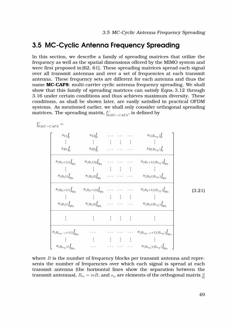
3.5 MC-Cyclic Antenna Frequency Spreading
3.5 MC-Cyclic Antenna Frequency Spreading
In this section, we describe a family of spreading matrices that utilize thefrequency as well as the spatial dimensions offered by the MIMO system andwere first proposed in [62, 61]. These spreading matrices spread each signalover all transmit antennas and over a set of frequencies at each transmitantenna. These frequency sets are different for each antenna and thus thename MC-CAFS: multi-carrier cyclic antenna frequency spreading. We shallshow that this family of spreading matrices can satisfy Eqns. 3.12 through3.16 under certain conditions and thus achieves maximum diversity. Theseconditions, as shall be shown later, are easily satisfied in practical OFDMsystems. As mentioned earlier, we shall only consider orthogonal spreadingmatrices. The spreading matrix, U
MC−CAFS, is defined by
UMC−CAFS
=
s11I s12I . . . . . . . . . s1(BnT)I
......
......
......
sB1I sB2I . . . . . . . . . sB(BnT)I
s(B1+1)1Ip1s(B11)2Ip1
. . . . . . . . . s(B1+1)(BnT)Ip1
......
......
......
s(B2)1Ip1s(B2)2Ip1
. . . . . . . . . s(B2)(BnT)Ip1
s(B2+1)1Ip2s(B2+1)2Ip2
. . . . . . . . . s(B2+1)(BnT)Ip2
......
......
......
s(B3)1Ip2s(B3)2Ip2
. . . . . . . . . s(B3)(BnT)Ip2
......
......
......
s(BnT−1+1)1Ipn. . . . . . . . . . . . s(BnT−1+1)(BnT
)Ipn
......
......
......
s(BnT)1Ipn
. . . . . . . . . . . . s(BnT)(BnT
)Ipn
(3.21)
where B is the number of frequency blocks per transmit antenna and repre-sents the number of frequencies over which each signal is spread at eachtransmit antenna (the horizontal lines show the separation between thetransmit antennas), Bm = mB, and sij are elements of the orthogonal matrix S
49
3 Spreading
(i. e. SHS = I) of size (nTB)×(nTB). I is identity matrices of size (N/B)×(N/B)and I
piis its i-th permutation. The permutations imply that each signal is
spread over different frequencies at each transmit antenna and ensure thatthe first criterion (Eqn. 3.12) is satisfied [62]. Note that the number of allowedpermutations, n, must satisfy n ≤ (nT − 1) (i. e. no permutation should re-peat), else U
MC−CAFSwill loose its orthogonality. This condition translates to
(N/B) ≥ nT and gives an upper bound for B:
B ≤ N/nT. (3.22)
In addition, to insure that Eqn. 3.15 is satisfied, B must be lower boundedby:
B ≥ L (3.23)
This can be proven by closely looking at the exponential term of Eqn. 3.13.At any transmit antenna, this equation is satisfied if we spread over a subsetof frequencies such that:
∑
k=Si1⊂S1
cos(k2π
N(l − m)) = 0,
∑
k=Si1⊂S1
sin(k2π
N(l − m)) = 0, (3.24)
where∑
i Si1 = S1. Note that Eqns 3.24 are readily satisfied for k = S1. How-ever, choosing k = S1 contradicts with Criterion 1. Without loss of generality,we consider the case where N is an even integer. This is applicable to OFDMsystems where the fast Fourier transform (FFT) and the inverse fast Fouriertransform (IFFT) are employed. Accordingly, Si1 include the subset of fre-quencies such that
∆k2π
N(l − m) = π, (3.25)
∆k =
⌈ N2(l−m)
⌉ if (l − m) even
N2
if (l − m) odd
, (3.26)
where ⌈x⌉ rounds x towards infinity. Thus, to insure that Eqn. 3.15 is satis-fied, any one symbol must be spread over an integer number of B frequenciessatisfying
B = max{ N
∆k} ≥ L. (3.27)
50
3.5 MC-Cyclic Antenna Frequency Spreading
The MC-CAFS spreading would therefore achieve maximum diversity, if Bsatisfies the following criteria
L ≤ B ≤ N
nT
. (3.28)
Note that for a given N , nT and L, there is a set of B values (i. e. set ofspreading matrices) that would satisfy eqns. 3.12 to 3.16. In addition, Bmust also be chosen such that N/B is an integer.
To summarize, it is clear that for Eqn. 3.13 to be satisfied, it is enough toinsure that any symbol is spread over the adequate number of frequencies ofits corresponding transmit antenna (Eqn.3.15). The choice of the subset iT ⊂S2= {1, . . . , nT} does not affect the equality in Eqn. 3.13, but affects validity ofEqn. 3.16. By choosing iT =S2, Eqn. 3.16 is satisfied. That is, although thesymbols need not be spread over all frequencies, they must be spread overall antennas. Through the use of the permutations, MC-CAFS satisfies thisrequirement without violating the first criterion.
Example 1
For example, consider a nR × nT MIMO-OFDM system with N = 8 and forthe cases, L = 2, L = 3 and L = 4. For L = 2, the maximum possible valuefor (l − m) = 1, for L = 3 and L = 4, they are (l − m) = 2 and 3 respectively.
Fig. 3.3 shows the values of E(k) = e−j2π(k−1)(l−m)
N for (l − m) = 1, 2 and 3. Forevery point on the circle, there is another point satisfying E(k + ∆k) = −E(k)(separated by an angle of π). For L = 2, ∆k = 4, while for L = 3 and (l−m) = 2,∆k = 2. Thus, for L = 2, it would be enough to spread over B = 2 frequenciesseparated by ∆k = 4 and over B = 4 frequencies separated by ∆k = 2 forL = 3. For L = 4 and (l − m) = 3, ∆k = 4 and accordingly B = 2 would besufficient. However, since the sum in Eqn. 3.15 also includes the sum for(l − m) = 2, thus ∆k = 2 must be chosen. Also note that in the case of L = 3,the condition for (l − m) = 1 is automatically satisfied if ∆k = 2, that is B = 4.
Example 2
Consider a MIMO-OFDM channel with nT = nR = 2, L = 2 and N = 4. Thediagonal elements of R before spreading for the first antenna at k = 1 and 3
51
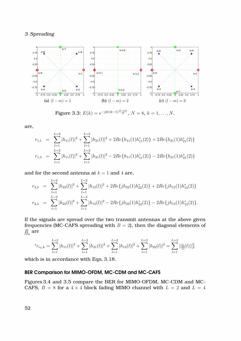
3 Spreading
−1 −0.75 −0.5 −0.25 0 0.25 0.5 0.75 1−1
−0.75
−0.5
−0.25
0
0.25
0.5
0.75
1
k=1
k=2 k=3 k=4
k=5
k=6 k=7
k=8
(a) (l − m) = 1
−1 −0.75 −0.5 −0.25 0 0.25 0.5 0.75 1−1
−0.75
−0.5
−0.25
0
0.25
0.5
0.75
1
k=1,5
k=2,6
k=3,7
k=4,8
(b) (l − m) = 2
−1 −0.75 −0.5 −0.25 0 0.25 0.5 0.75 1−1
−0.75
−0.5
−0.25
0
0.25
0.5
0.75
1
k=1
k=2
k=3
k=4
k=5
k=6
k=7
k=8
(c) (l − m) = 3
Figure 3.3: E(k) = e−j2π(k−1)(l−m)
N , N = 8, k = 1, . . . , N .
are,
r1,1 =L=2∑
l=1
|h11(l)|2 +L=2∑
l=1
|h21(l)|2 + 2Re{h11(1)h∗11(2)} + 2Re{h21(1)h∗
21(2)}
r1,3 =L=2∑
l=1
|h11(l)|2 +L=2∑
l=1
|h21(l)|2 − 2Re{h11(1)h∗11(2)} − 2Re{h21(1)h∗
21(2)}
and for the second antenna at k = 1 and 4 are,
r2,2 =L=2∑
l=1
|h22(l)|2 +L=2∑
l=1
|h12(l)|2 + 2Re{jh22(1)h∗22(2)} + 2Re{jh12(1)h∗
12(2)}
r2,4 =L=2∑
l=1
|h22(l)|2 +L=2∑
l=1
|h12(l)|2 − 2Re{jh22(1)h∗22(2)} − 2Re{jh12(1)h∗
12(2)}.
If the signals are spread over the two transmit antennas at the above givenfrequencies (MC-CAFS spreading with B = 2), then the diagonal elements ofR
sare
sriT,k =L=2∑
l=1
|h11(l)|2 +L=2∑
l=1
|h21(l)|2 +L=2∑
l=1
|h12(l)|2 +L=2∑
l=1
|h22(l)|2 =L=2∑
l=1
||h(l)||2F
which is in accordance with Eqn. 3.18.
BER Comparison for MIMO-OFDM, MC-CDM and MC-CAFS
Figures 3.4 and 3.5 compare the BER for MIMO-OFDM, MC-CDM and MC-CAFS, B = 8 for a 4 × 4 block fading MIMO channel with L = 2 and L = 4
52
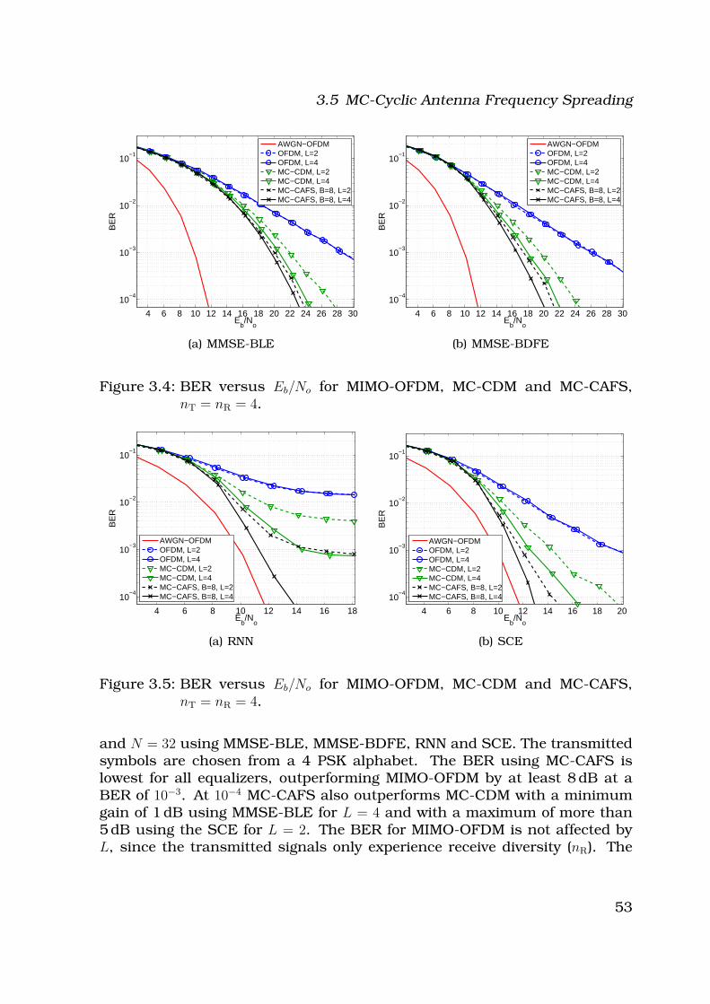
3.5 MC-Cyclic Antenna Frequency Spreading
4 6 8 10 12 14 16 18 20 22 24 26 28 30
10−4
10−3
10−2
10−1
Eb/N
o
BE
R
AWGN−OFDMOFDM, L=2OFDM, L=4MC−CDM, L=2MC−CDM, L=4MC−CAFS, B=8, L=2MC−CAFS, B=8, L=4
(a) MMSE-BLE
4 6 8 10 12 14 16 18 20 22 24 26 28 30
10−4
10−3
10−2
10−1
Eb/N
o
BE
R
AWGN−OFDMOFDM, L=2OFDM, L=4MC−CDM, L=2MC−CDM, L=4MC−CAFS, B=8, L=2MC−CAFS, B=8, L=4
(b) MMSE-BDFE
Figure 3.4: BER versus Eb/No for MIMO-OFDM, MC-CDM and MC-CAFS,nT = nR = 4.
4 6 8 10 12 14 16 18
10−4
10−3
10−2
10−1
Eb/N
o
BE
R
AWGN−OFDMOFDM, L=2OFDM, L=4MC−CDM, L=2MC−CDM, L=4MC−CAFS, B=8, L=2MC−CAFS, B=8, L=4
(a) RNN
4 6 8 10 12 14 16 18 20
10−4
10−3
10−2
10−1
Eb/N
o
BE
R
AWGN−OFDMOFDM, L=2OFDM, L=4MC−CDM, L=2MC−CDM, L=4MC−CAFS, B=8, L=2MC−CAFS, B=8, L=4
(b) SCE
Figure 3.5: BER versus Eb/No for MIMO-OFDM, MC-CDM and MC-CAFS,nT = nR = 4.
and N = 32 using MMSE-BLE, MMSE-BDFE, RNN and SCE. The transmittedsymbols are chosen from a 4 PSK alphabet. The BER using MC-CAFS islowest for all equalizers, outperforming MIMO-OFDM by at least 8 dB at aBER of 10−3. At 10−4 MC-CAFS also outperforms MC-CDM with a minimumgain of 1 dB using MMSE-BLE for L = 4 and with a maximum of more than5 dB using the SCE for L = 2. The BER for MIMO-OFDM is not affected byL, since the transmitted signals only experience receive diversity (nR). The
53

3 Spreading
small shift between the BER curve for L = 2 and L = 4 is only due to thecyclic prefix. The diversity gain (steeper BER curve), for all L, using MC-CAFS compared to MC-CDM is most obvious when the SCE or RNN equalizersare employed (see Fig. 3.5). In addition, the BER curve for MC-CAFS forL = 4 is steeper than that for L = 2 due to increased diversity. This resultis not as obvious for MMSE-BLE and MMSE-BDFE for L = 4. However, athigher Eb/No, the difference in the BER curve slopes might become morenoticeable. The RNN equalizer is sensitive to interference and can sufferfrom an error floor (cf. Chap. 2). Here, the error floor is observed to occurat around 14 dB. Increasing the Eb/No beyond 14 dB does not lead to lowerBER. The BER performance for the RNN equalizer benefits the most fromMC-CAFS spreading. The error floor drops by at least one decade for L = 2compared to OFDM. For L = 4 the error floor drops even further. Due tothe high interference present, the performance of the MMSE-BLE and theMMSE-BDFE is in general worse than that of the RNN and SCE. Even withMC-CAFS spreading, the BER curves are at least 8 dB from the AWGN-OFDMcurve at a BER of 10−4.
0 0.1 0.2 0.3 0.4 0.5 0.6 0.7 0.8 0.9
10−4
10−3
10−2
10−1
ρ
BE
R
Eb/N
o=14dB
OFDMMC−CDMMC−CAFS,B=8
(a) RNN
0 0.1 0.2 0.3 0.4 0.5 0.6 0.7 0.8 0.9
10−5
10−4
10−3
10−2
10−1
ρ
BE
R
Eb/N
o=14dB
OFDMMC−CDMMC−CAFS,B=8
(b) SCE
Figure 3.6: BER versus ρTx,exp = ρRx,exp = ρ at Eb/No = 14 dB for MIMO-OFDM,MC-CDM and MC-CAFS, nT = nR = 4, L = 4.
Figure 3.6 shows the BER versus ρ (ρTx,exp = ρRx,exp = ρ) assuming an expo-nential correlation model at Eb/No = 14 dB for RNN and SCE using 4 PSK. TheBER for MC-CAFS is the lowest for low to moderate correlation values (ρ ≤ 0.6for SCE and ρ ≤ 0.3 for RNN). In case of the RNN equalizer, both MC-CDMand MC-CAFS have comparable performance for ρ ≥ 0.3. For ρ > 0.5, thesystem performance for MC-CAFS, MC-CDM and OFDM is poor and the BERcurves lie close together with OFDM leading to slightly lower BERs. Similarly
54
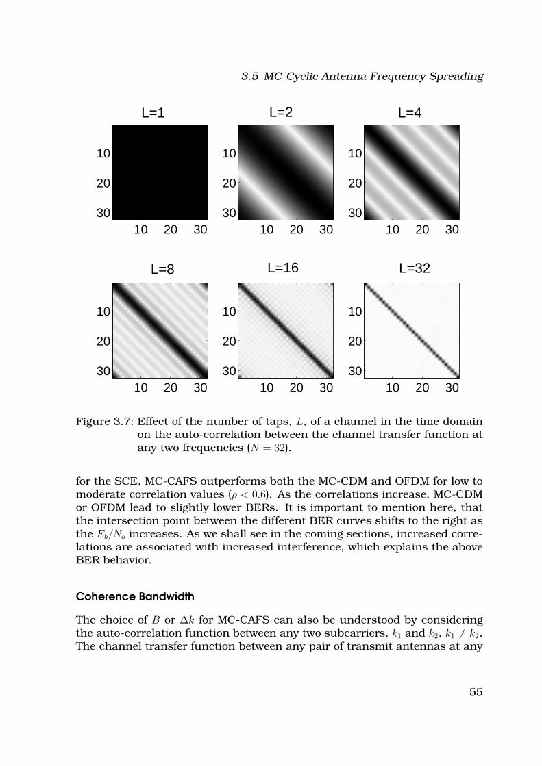
3.5 MC-Cyclic Antenna Frequency Spreading
10 20 30
10
20
3010 20 30
10
20
3010 20 30
10
20
30
10 20 30
10
20
3010 20 30
10
20
3010 20 30
10
20
30
L=1 L=2 L=4
L=8 L=16 L=32
Figure 3.7: Effect of the number of taps, L, of a channel in the time domainon the auto-correlation between the channel transfer function atany two frequencies (N = 32).
for the SCE, MC-CAFS outperforms both the MC-CDM and OFDM for low tomoderate correlation values (ρ < 0.6). As the correlations increase, MC-CDMor OFDM lead to slightly lower BERs. It is important to mention here, thatthe intersection point between the different BER curves shifts to the right asthe Eb/No increases. As we shall see in the coming sections, increased corre-lations are associated with increased interference, which explains the aboveBER behavior.
Coherence Bandwidth
The choice of B or ∆k for MC-CAFS can also be understood by consideringthe auto-correlation function between any two subcarriers, k1 and k2, k1 6= k2.The channel transfer function between any pair of transmit antennas at any
55
3 Spreading
subcarrier k1 can be written as follows
Hij(k1) =L∑
l=1
hij(l)e−j 2π
Nk1(l−1). (3.29)
The auto-correlation function between between any two subcarriers, assum-ing independent fading paths, can thus be given by
E{Hij(k1)H∗ij(k2)} =
L∑
l=1
E{|hij(l)2|}e−j 2π
N∆k(l−1), (3.30)
where ∆k = k2−k1. Assuming a uniform power profile, i. e. E{|hij(l)2|} = σ2, ∀ l,
then
E{Hij(k1)H∗ij(k2)} = σ2
L∑
l=1
e−j 2πN
∆k(l−1). (3.31)
Now we find ∆k for which Eqn. 3.31 is equal to zero. In other words, thecorrelations are zero, if
L∑
l=1
cos2π
N∆k(l − 1) = 0,
L∑
l=1
sin2π
N∆k(l − 1) = 0,
(3.32)
which is satisfied if
∆k =N
L. (3.33)
The value of ∆k in Eqn. 3.33 can also be interpreted as the coherence band-width if we assume uncorrelated scattering (US) of the channel taps withequal PDP. That is, the delay spread in the channel have independent fading[22]. The subcarriers with spacing larger than the coherence bandwidth ex-perience independent fading. To achieve maximum diversity it is thus enoughto spread over N/Bc = N/∆k frequencies separated by the coherence band-width, i. e. to spread over all coherence bandwidths. Figure 3.7 shows theauto-correlation between any two subcarriers for different number of channeltaps, L. As the number of channel taps increases, the coherence Bandwidthdecreases. For N = L, the coherence Bandwidth is zero.
Even for non-equal PDP, Eqns. 3.32 are still satisfied for ∆k = N/L. How-ever, in this case ∆k is not necessarily equal to the coherence bandwidth. Incase of non-equal PDP, where some of the taps have more power than others,
56
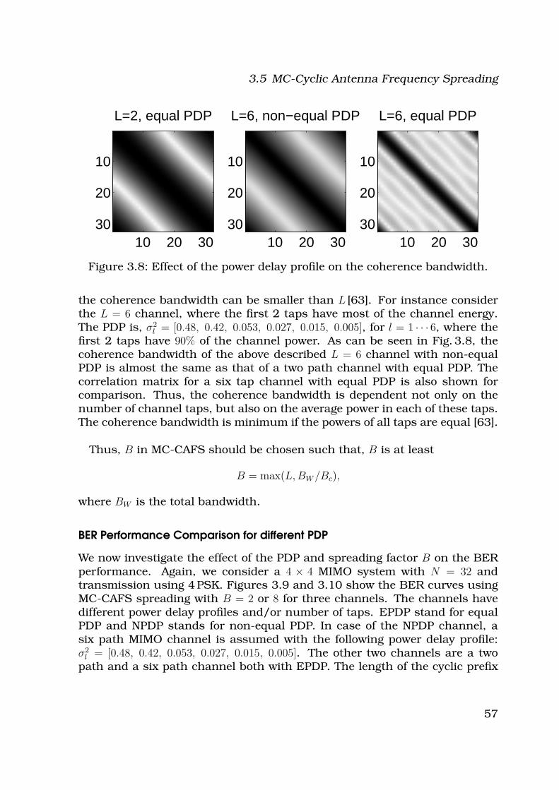
3.5 MC-Cyclic Antenna Frequency Spreading
L=2, equal PDP
10 20 30
10
20
30
L=6, non−equal PDP
10 20 30
10
20
30
L=6, equal PDP
10 20 30
10
20
30
Figure 3.8: Effect of the power delay profile on the coherence bandwidth.
the coherence bandwidth can be smaller than L [63]. For instance considerthe L = 6 channel, where the first 2 taps have most of the channel energy.The PDP is, σ2
l = [0.48, 0.42, 0.053, 0.027, 0.015, 0.005], for l = 1 · · · 6, where thefirst 2 taps have 90% of the channel power. As can be seen in Fig. 3.8, thecoherence bandwidth of the above described L = 6 channel with non-equalPDP is almost the same as that of a two path channel with equal PDP. Thecorrelation matrix for a six tap channel with equal PDP is also shown forcomparison. Thus, the coherence bandwidth is dependent not only on thenumber of channel taps, but also on the average power in each of these taps.The coherence bandwidth is minimum if the powers of all taps are equal [63].
Thus, B in MC-CAFS should be chosen such that, B is at least
B = max(L,BW /Bc),
where BW is the total bandwidth.
BER Performance Comparison for different PDP
We now investigate the effect of the PDP and spreading factor B on the BERperformance. Again, we consider a 4 × 4 MIMO system with N = 32 andtransmission using 4 PSK. Figures 3.9 and 3.10 show the BER curves usingMC-CAFS spreading with B = 2 or 8 for three channels. The channels havedifferent power delay profiles and/or number of taps. EPDP stand for equalPDP and NPDP stands for non-equal PDP. In case of the NPDP channel, asix path MIMO channel is assumed with the following power delay profile:σ2
l = [0.48, 0.42, 0.053, 0.027, 0.015, 0.005]. The other two channels are a twopath and a six path channel both with EPDP. The length of the cyclic prefix
57
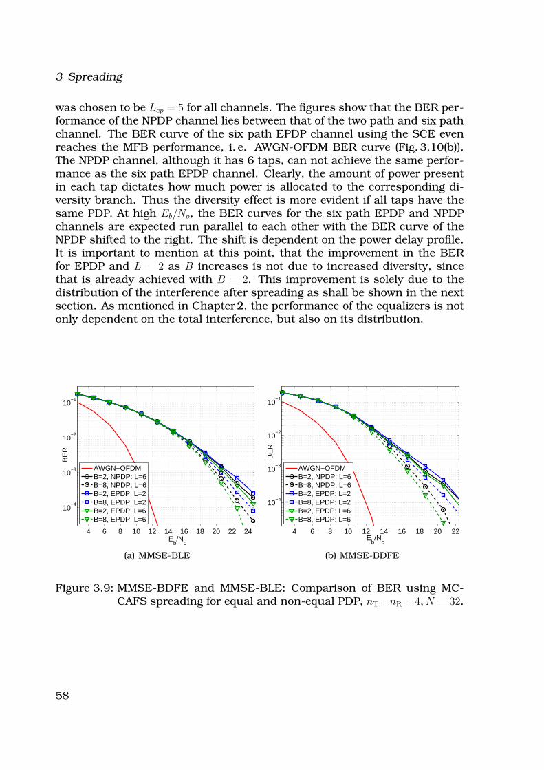
3 Spreading
was chosen to be Lcp = 5 for all channels. The figures show that the BER per-formance of the NPDP channel lies between that of the two path and six pathchannel. The BER curve of the six path EPDP channel using the SCE evenreaches the MFB performance, i. e. AWGN-OFDM BER curve (Fig. 3.10(b)).The NPDP channel, although it has 6 taps, can not achieve the same perfor-mance as the six path EPDP channel. Clearly, the amount of power presentin each tap dictates how much power is allocated to the corresponding di-versity branch. Thus the diversity effect is more evident if all taps have thesame PDP. At high Eb/No, the BER curves for the six path EPDP and NPDPchannels are expected run parallel to each other with the BER curve of theNPDP shifted to the right. The shift is dependent on the power delay profile.It is important to mention at this point, that the improvement in the BERfor EPDP and L = 2 as B increases is not due to increased diversity, sincethat is already achieved with B = 2. This improvement is solely due to thedistribution of the interference after spreading as shall be shown in the nextsection. As mentioned in Chapter 2, the performance of the equalizers is notonly dependent on the total interference, but also on its distribution.
4 6 8 10 12 14 16 18 20 22 24
10−4
10−3
10−2
10−1
Eb/N
o
BE
R
AWGN−OFDMB=2, NPDP: L=6B=8, NPDP: L=6B=2, EPDP: L=2B=8, EPDP: L=2B=2, EPDP: L=6B=8, EPDP: L=6
(a) MMSE-BLE
4 6 8 10 12 14 16 18 20 22
10−4
10−3
10−2
10−1
Eb/N
o
BE
R
AWGN−OFDMB=2, NPDP: L=6B=8, NPDP: L=6B=2, EPDP: L=2B=8, EPDP: L=2B=2, EPDP: L=6B=8, EPDP: L=6
(b) MMSE-BDFE
Figure 3.9: MMSE-BDFE and MMSE-BLE: Comparison of BER using MC-CAFS spreading for equal and non-equal PDP, nT =nR = 4, N = 32.
58
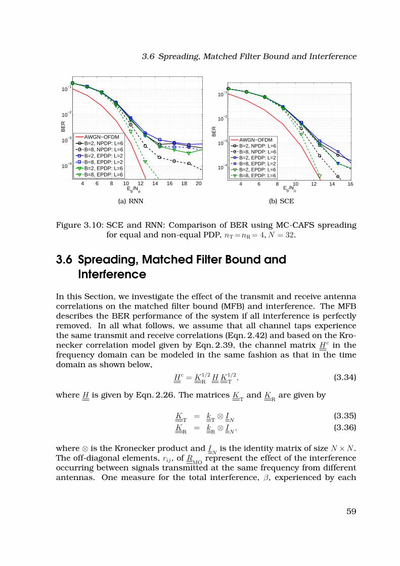
3.6 Spreading, Matched Filter Bound and Interference
4 6 8 10 12 14 16 18 20
10−4
10−3
10−2
10−1
Eb/N
o
BE
R
AWGN−OFDMB=2, NPDP: L=6B=8, NPDP: L=6B=2, EPDP: L=2B=8, EPDP: L=2B=2, EPDP: L=6B=8, EPDP: L=6
(a) RNN
4 6 8 10 12 14 16
10−4
10−3
10−2
10−1
Eb/N
o
BE
R
AWGN−OFDMB=2, NPDP: L=6B=8, NPDP: L=6B=2, EPDP: L=2B=8, EPDP: L=2B=2, EPDP: L=6B=8, EPDP: L=6
(b) SCE
Figure 3.10: SCE and RNN: Comparison of BER using MC-CAFS spreadingfor equal and non-equal PDP, nT =nR = 4, N = 32.
3.6 Spreading, Matched Filter Bound and
Interference
In this Section, we investigate the effect of the transmit and receive antennacorrelations on the matched filter bound (MFB) and interference. The MFBdescribes the BER performance of the system if all interference is perfectlyremoved. In all what follows, we assume that all channel taps experiencethe same transmit and receive correlations (Eqn. 2.42) and based on the Kro-necker correlation model given by Eqn. 2.39, the channel matrix Hc in thefrequency domain can be modeled in the same fashion as that in the timedomain as shown below,
Hc = K1/2
RH K1/2
T, (3.34)
where H is given by Eqn. 2.26. The matrices KT
and KR
are given by
KT
= kT⊗ I
N(3.35)
KR
= kR⊗ I
N, (3.36)
where ⊗ is the Kronecker product and IN
is the identity matrix of size N ×N .The off-diagonal elements, rij, of R
MOrepresent the effect of the interference
occurring between signals transmitted at the same frequency from differentantennas. One measure for the total interference, β, experienced by each
59
3 Spreading
transmit symbol is defined as follows [64, 65],
β =1
nTN
∑
i6=j
|rij|2 ≥ 0, (3.37)
where rij are the off-diagonal elements of R, and R being either RMO
or RS.
Another measure for the total interference would be
β1/2 =1
nTN
∑
i6=j
|rij| ≥ 0, (3.38)
which is simply the sum of the absolute values of the off-diagonal elements.In what follows, we will concentrate on β, but we shall also consider β1/2 lateron. The variance of the subchannel power, α, from the mean r, is given by[64, 65]
α =1
nTN
∑
i
(rii − r)2 ≥ 0, (3.39)
where rii are the diagonal elements of R and
r =1
NnT
NnT∑
i=1
rii. (3.40)
α gives a measure for the MFB bound, with a larger value of α correspondingto a worse MFB and vice versa. If α = 0, then all signals undergo the sameamount of fading. In this case, the MFB is governed by the amount of diver-sity and correlations present in the channel as was discussed in Sec. 3.1.
From the above definitions of α and β, we can write
α + β =||R||2FnTN
− r2, (3.41)
where ||R||2F is the Frobenius norm of R. Since, we only consider orthogonalspreading matrices, neither ||R||2F nor r change after spreading. Thus, theindividual values of α and β can change, but their sum remains constant. Asmentioned above, a large α value corresponds to a poor MFB and a large βvalue to high interference. Yet, since α and β are both positive, it is obviousfrom Eqn. 3.41 that if α increases, then β decreases and vice versa. Thesum α + β = 0, if and only if R is a scaled identity matrix, which is the idealcase. MC-CAFS spreading leads to α = 0 and β thus reaches its maximum
value(
β =||R||2FnTN
− r2)
. However, as we have seen in the previous Sections,the BER performance of MC-CAFS is still better than for other spreadingmatrices due to increased diversity (improved MFB). On the other hand, if
60
3.6 Spreading, Matched Filter Bound and Interference
perfect channel knowledge is present at the transmitter, we can use theeigenvectors of the channel correlation matrix, R
MO, as precoding matrices
and thus diagonalizing the channel matrix. In this case, β = 0, and α reachesits maximum value. Precoding will be discussed in more detail in the nextChapter.
Equation 3.41 gives the values of α + β for one channel realization. Theexpected value of the sum in Eqn. 3.41 is thus,
E{α + β} = E{α} + E{β} =E{||R||2F}
nTN− (1 + var(r)), (3.42)
where E{r2} = (E{r})2 + var(r) = 1 + var(r). We have shown in Appendix 3.A.2,that var (r) = 1/Ψ(R
v), where Ψ(R
v) is given by Eqn. 2.51 and R
vby Eqn. 2.53.
Accordingly, based on derivations in Appendix 3.A.2, we obtain
E{α} + E{β} =nT
nR
+2nT
n2R
nR−1∑
i=1
(nR − i)|ρRxi|2 +2
nT
nT−1∑
j=1
(nT − j)|ρTxj|2 − var(r),
(3.43)
where ρRxi and ρTxj are the elements of kR
and kT
respectively. For the un-spread MIMO-OFDM, by expanding Eqn. 3.39, we get
α =1
nTN
nTN∑
i=1
(rii − r)2 =1
nTN
nTN∑
i=1
(r2ii + r2 − 2rrii) =
1
nTN
nTN∑
i=1
r2ii − r2 (3.44)
Thus,
E{α} =1
nR
+2
n2R
nR−1∑
i=1
(nR − i)|ρRxi|2 − var(r). (3.45)
Note that the var(r) represents the effect of the different fading occurring inthe different MIMO channels, for example, frequency selectivity.
The expected value of β is
E{β} = (nT − 1)
(
1
nR
+2
n2R
nR−1∑
i=1
(nR − i)|ρRxi|2)
+2
nT
nT−1∑
j=1
(nT − j)|ρTxj|2. (3.46)
For equal correlation coefficients (ρm = ρ, ∀m ), Eqn. 3.43 reduces to
E{α + β} =nT
nR
+nT
nR
(nR − 1)|ρRx|2 + (nT − 1)|ρTx|2 − var(r), (3.47)
61
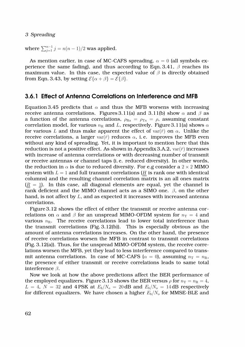
3 Spreading
where∑n−1
j=1 j = n(n − 1)/2 was applied.
As mention earlier, in case of MC-CAFS spreading, α = 0 (all symbols ex-perience the same fading), and thus according to Eqn. 3.41, β reaches itsmaximum value. In this case, the expected value of β is directly obtainedfrom Eqn. 3.43, by setting E{α + β} = E{β}.
3.6.1 Effect of Antenna Correlations on Interference and MFB
Equation 3.45 predicts that α and thus the MFB worsens with increasingreceive antenna correlations. Figures 3.11(a) and 3.11(b) show α and β asa function of the antenna correlations, ρRx = ρTx = ρ, assuming constantcorrelation model, for various nR and L, respectively. Figure 3.11(a) shows αfor various L and thus make apparent the effect of var(r) on α. Unlike thereceive correlations, a larger var(r) reduces α, i. e. improves the MFB evenwithout any kind of spreading. Yet, it is important to mention here that thisreduction is not a positive effect. As shown in Appendix 3.A.2, var(r) increaseswith increase of antenna correlations or with decreasing number of transmitor receive antennas or channel taps (i. e. reduced diversity). In other words,the reduction in α is due to reduced diversity. For e.g consider a 2 × 2 MIMOsystem with L = 1 and full transmit correlations (H is rank one with identicalcolumns) and the resulting channel correlation matrix is an all ones matrix(R = 1). In this case, all diagonal elements are equal, yet the channel isrank deficient and the MIMO channel acts as a SIMO one. β, on the otherhand, is not affect by L, and as expected it increases with increased antennacorrelations.
Figure 3.12 shows the effect of either the transmit or receive antenna cor-relations on α and β for an unspread MIMO-OFDM system for nT = 4 andvarious nR. The receive correlations lead to lower total interference thanthe transmit correlations (Fig. 3.12(b)). This is especially obvious as theamount of antenna correlations increases. On the other hand, the presenceof receive correlations worsen the MFB in contrast to transmit correlations(Fig. 3.12(a)). Thus, for the unspread MIMO-OFDM system, the receive corre-lations worsen the MFB, yet they lead to less interference compared to trans-mit antenna correlations. In case of MC-CAFS (α = 0), assuming nT = nR,the presence of either transmit or receive correlations leads to same totalinterference β.
Now we look at how the above predictions affect the BER performance ofthe employed equalizers. Figure 3.13 shows the BER versus ρ for nT = nR = 4,L = 4, N = 32 and 4 PSK at Eb/No = 20 dB and Eb/No = 14 dB respectivelyfor different equalizers. We have chosen a higher Eb/No for MMSE-BLE and
62
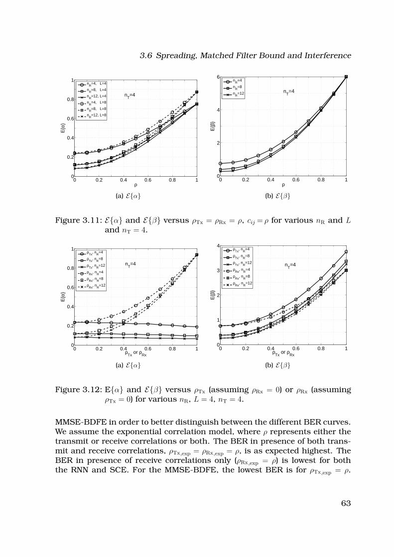
3.6 Spreading, Matched Filter Bound and Interference
0 0.2 0.4 0.6 0.8 10
0.2
0.4
0.6
0.8
1
ρ
E{α
}
nT=4
n
R=4, L=4
nR
=8, L=4
nR
=12, L=4
nR
=4, L=8
nR
=8, L=8
nR
=12, L=8
(a) E{α}
0 0.2 0.4 0.6 0.8 10
2
4
6
ρ
E{β
}
nT=4
n
R=4
nR
=8
nR
=12
(b) E{β}
Figure 3.11: E{α} and E{β} versus ρTx = ρRx = ρ, cij = ρ for various nR and Land nT = 4.
0 0.2 0.4 0.6 0.8 10
0.2
0.4
0.6
0.8
1
ρTx
or ρRx
E{α
}
nT=4
ρ
Tx, n
R=4
ρTx
, nR
=8
ρTx
, nR
=12
ρRx
, nR
=4
ρRx
, nR
=8
ρRx
, nR
=12
(a) E{α}
0 0.2 0.4 0.6 0.8 10
1
2
3
4
ρTx
or ρRx
E{β
}
nT=4
ρ
Tx, n
R=4
ρTx
, nR
=8
ρTx
, nR
=12
ρRx
, nR
=4
ρRx
, nR
=8
ρRx
, nR
=12
(b) E{β}
Figure 3.12: E{α} and E{β} versus ρTx (assuming ρRx = 0) or ρRx (assumingρTx = 0) for various nR, L = 4, nT = 4.
MMSE-BDFE in order to better distinguish between the different BER curves.We assume the exponential correlation model, where ρ represents either thetransmit or receive correlations or both. The BER in presence of both trans-mit and receive correlations, ρTx,exp = ρRx,exp = ρ, is as expected highest. TheBER in presence of receive correlations only (ρRx,exp = ρ) is lowest for boththe RNN and SCE. For the MMSE-BDFE, the lowest BER is for ρTx,exp = ρ.
63
3 Spreading
0 0.2 0.4 0.6 0.810
−3
10−2
10−1
ρ
BE
R
Eb/N
o=20dB
OFDM, ρ=ρTx,exp
=ρRx,exp
OFDM, ρ=ρTx,exp
OFDM, ρ=ρRx,exp
(a) MMSE-BLE
0 0.2 0.4 0.6 0.810
−3
10−2
10−1
ρ
BE
R
Eb/N
o=20dB
OFDM, ρ=ρTx,exp
=ρRx,exp
OFDM, ρ=ρTx,exp
OFDM, ρ=ρRx,exp
(b) MMSE-BDFE
0 0.1 0.2 0.3 0.4 0.5 0.6 0.7 0.8 0.910
−3
10−2
10−1
ρ
BE
R
Eb/N
o=14dB
OFDM, ρ=ρTx,exp
=ρRx,exp
OFDM, ρ=ρTx,exp
OFDM, ρ=ρRx,exp
(c) RNN
0 0.1 0.2 0.3 0.4 0.5 0.6 0.7 0.8 0.910
−3
10−2
10−1
ρ
BE
R
Eb/N
o=14dB
OFDM, ρ=ρTx,exp
=ρRx,exp
OFDM, ρ=ρTx,exp
OFDM, ρ=ρRx,exp
(d) SCE
Figure 3.13: MIMO-OFDM: Comparison of BER in presence of either transmitor receive correlations or both for nT = nR = 4, L = 4 and N = 32.
In presence of either transmit or receive correlations, the MMSE-BLE BERcurves are almost identical for both cases. As afore mentioned, receive corre-lations, although worsen the MFB, leads to lower interference, which seemsto play a more important factor in the system performance at high antennacorrelations for the RNN and SCE. For the MMSE-BDFE, the MFB appears toplay the more important role. This may be due to the fact the MMSE-BDFEis prone to propagation errors.
Figure 3.14 shows E{α + β} for different correlation models: constant,exponential and complex exponential correlation model. We assume thepresence of antenna correlations at both the transmitter and receiver withρRx = ρTx = ρ. Based on the definition of the correlation measure in Sec. 2.4.2,
64
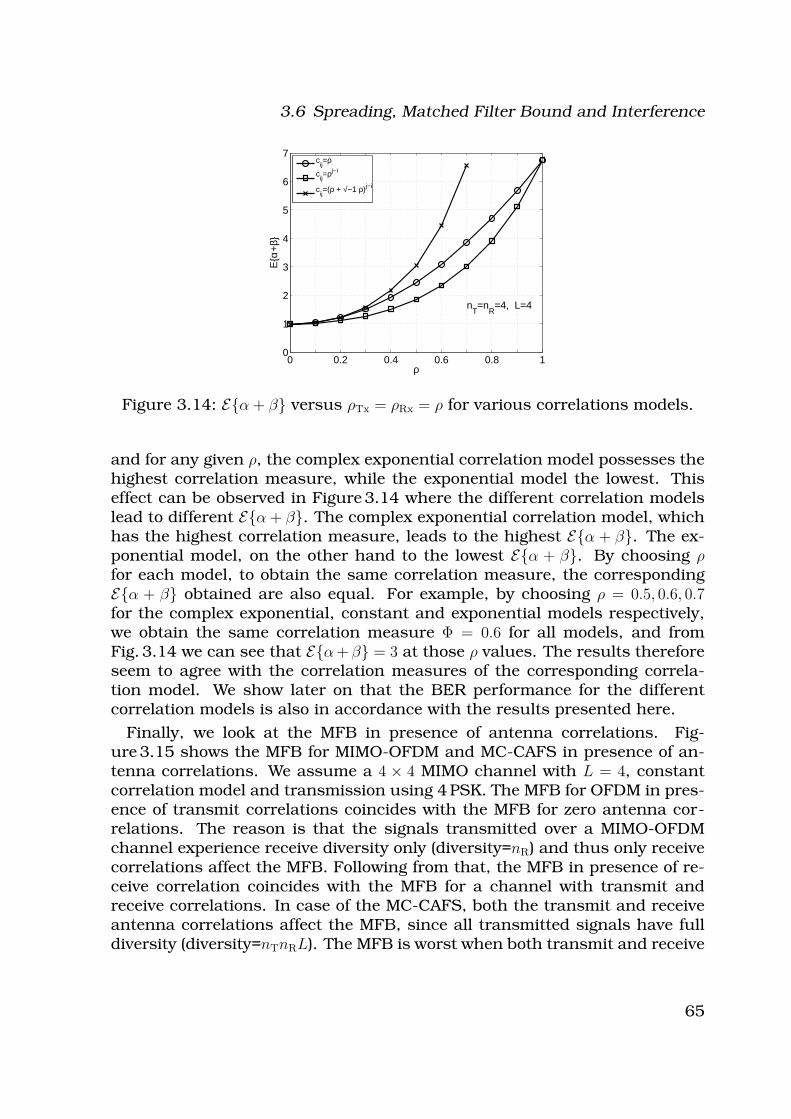
3.6 Spreading, Matched Filter Bound and Interference
0 0.2 0.4 0.6 0.8 10
1
2
3
4
5
6
7
ρ
E{α
+β}
nT=n
R=4, L=4
c
ij=ρ
cij=ρj−i
cij=(ρ + √−1 ρ)j−i
Figure 3.14: E{α + β} versus ρTx = ρRx = ρ for various correlations models.
and for any given ρ, the complex exponential correlation model possesses thehighest correlation measure, while the exponential model the lowest. Thiseffect can be observed in Figure 3.14 where the different correlation modelslead to different E{α + β}. The complex exponential correlation model, whichhas the highest correlation measure, leads to the highest E{α + β}. The ex-ponential model, on the other hand to the lowest E{α + β}. By choosing ρfor each model, to obtain the same correlation measure, the correspondingE{α + β} obtained are also equal. For example, by choosing ρ = 0.5, 0.6, 0.7for the complex exponential, constant and exponential models respectively,we obtain the same correlation measure Φ = 0.6 for all models, and fromFig. 3.14 we can see that E{α + β} = 3 at those ρ values. The results thereforeseem to agree with the correlation measures of the corresponding correla-tion model. We show later on that the BER performance for the differentcorrelation models is also in accordance with the results presented here.
Finally, we look at the MFB in presence of antenna correlations. Fig-ure 3.15 shows the MFB for MIMO-OFDM and MC-CAFS in presence of an-tenna correlations. We assume a 4 × 4 MIMO channel with L = 4, constantcorrelation model and transmission using 4 PSK. The MFB for OFDM in pres-ence of transmit correlations coincides with the MFB for zero antenna cor-relations. The reason is that the signals transmitted over a MIMO-OFDMchannel experience receive diversity only (diversity=nR) and thus only receivecorrelations affect the MFB. Following from that, the MFB in presence of re-ceive correlation coincides with the MFB for a channel with transmit andreceive correlations. In case of the MC-CAFS, both the transmit and receiveantenna correlations affect the MFB, since all transmitted signals have fulldiversity (diversity=nTnRL). The MFB is worst when both transmit and receive
65
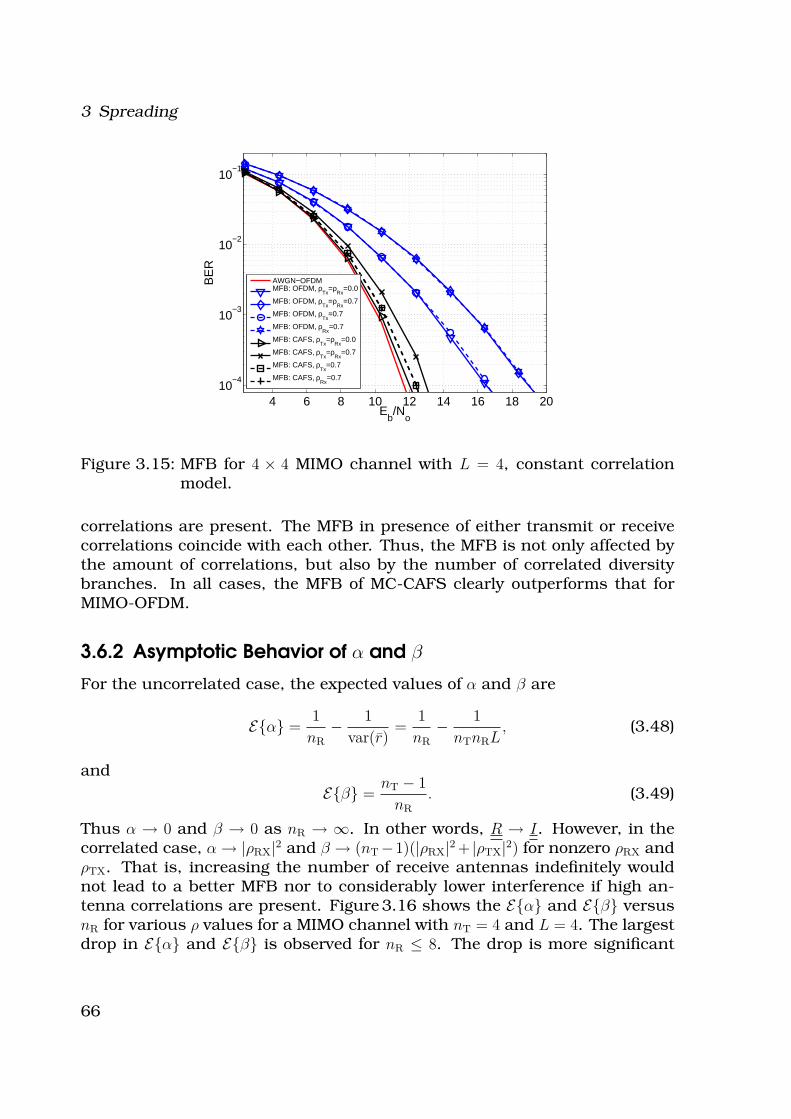
3 Spreading
4 6 8 10 12 14 16 18 2010
−4
10−3
10−2
10−1
Eb/N
o
BE
R
AWGN−OFDMMFB: OFDM, ρ
Tx=ρ
Rx=0.0
MFB: OFDM, ρTx
=ρRx
=0.7
MFB: OFDM, ρTx
=0.7
MFB: OFDM, ρRx
=0.7
MFB: CAFS, ρTx
=ρRx
=0.0
MFB: CAFS, ρTx
=ρRx
=0.7
MFB: CAFS, ρTx
=0.7
MFB: CAFS, ρRx
=0.7
Figure 3.15: MFB for 4 × 4 MIMO channel with L = 4, constant correlationmodel.
correlations are present. The MFB in presence of either transmit or receivecorrelations coincide with each other. Thus, the MFB is not only affected bythe amount of correlations, but also by the number of correlated diversitybranches. In all cases, the MFB of MC-CAFS clearly outperforms that forMIMO-OFDM.
3.6.2 Asymptotic Behavior of α and β
For the uncorrelated case, the expected values of α and β are
E{α} =1
nR
− 1
var(r)=
1
nR
− 1
nTnRL, (3.48)
and
E{β} =nT − 1
nR
. (3.49)
Thus α → 0 and β → 0 as nR → ∞. In other words, R → I. However, in thecorrelated case, α → |ρRX|2 and β → (nT−1)(|ρRX|2 + |ρTX|2) for nonzero ρRX andρTX. That is, increasing the number of receive antennas indefinitely wouldnot lead to a better MFB nor to considerably lower interference if high an-tenna correlations are present. Figure 3.16 shows the E{α} and E{β} versusnR for various ρ values for a MIMO channel with nT = 4 and L = 4. The largestdrop in E{α} and E{β} is observed for nR ≤ 8. The drop is more significant
66
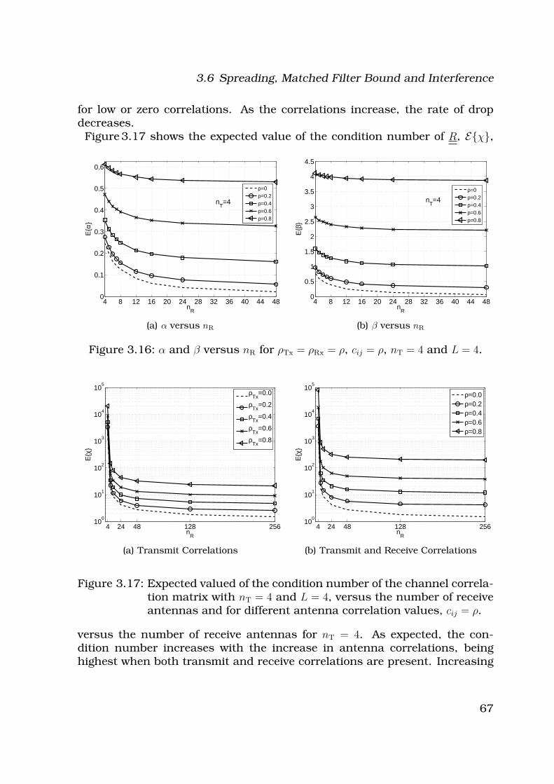
3.6 Spreading, Matched Filter Bound and Interference
for low or zero correlations. As the correlations increase, the rate of dropdecreases.Figure 3.17 shows the expected value of the condition number of R, E{χ},
4 8 12 16 20 24 28 32 36 40 44 480
0.1
0.2
0.3
0.4
0.5
0.6
nR
E{α
}
nT=4
ρ=0ρ=0.2ρ=0.4ρ=0.6ρ=0.8
(a) α versus nR
4 8 12 16 20 24 28 32 36 40 44 480
0.5
1
1.5
2
2.5
3
3.5
4
4.5
nR
E{β
}
nT=4
ρ=0ρ=0.2ρ=0.4ρ=0.6ρ=0.8
(b) β versus nR
Figure 3.16: α and β versus nR for ρTx = ρRx = ρ, cij = ρ, nT = 4 and L = 4.
4 24 48 128 25610
0
101
102
103
104
105
nR
E{χ
}
ρTx
=0.0
ρTx
=0.2
ρTx
=0.4
ρTx
=0.6
ρTx
=0.8
(a) Transmit Correlations
4 24 48 128 25610
0
101
102
103
104
105
nR
E{χ
}
ρ=0.0ρ=0.2ρ=0.4ρ=0.6ρ=0.8
(b) Transmit and Receive Correlations
Figure 3.17: Expected valued of the condition number of the channel correla-tion matrix with nT = 4 and L = 4, versus the number of receiveantennas and for different antenna correlation values, cij = ρ.
versus the number of receive antennas for nT = 4. As expected, the con-dition number increases with the increase in antenna correlations, beinghighest when both transmit and receive correlations are present. Increasing
67
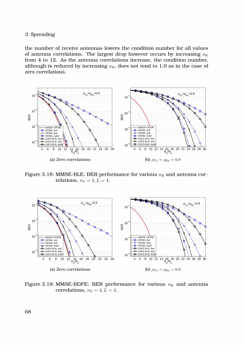
3 Spreading
the number of receive antennas lowers the condition number for all valuesof antenna correlations. The largest drop however occurs by increasing nR
from 4 to 12. As the antenna correlations increase, the condition number,although is reduced by increasing nR, does not tend to 1.0 as in the case ofzero correlations.
4 6 8 10 12 14 16 18 20 22 24 26 28
10−4
10−3
10−2
10−1
Eb/N
o
BE
R
ρTx
=ρRx
=0.0
AWGN−OFDMOFDM, 4x4OFDM, 4x8OFDM, 4x48CAFS B=8, 4x4CAFS B=8, 4x8CAFS B=8, 4x48
(a) Zero correlations
4 6 8 10 12 14 16 18 20 22 24 26 28 3010
−4
10−3
10−2
10−1
Eb/N
o
BE
R
ρTx
=ρRx
=0.8
AWGN−OFDMOFDM, 4x4OFDM, 4x8OFDM, 4x48CAFS B=8, 4x4CAFS B=8, 4x8CAFS B=8, 4x48
(b) ρTx = ρRx = 0.8
Figure 3.18: MMSE-BLE: BER performance for various nR and antenna cor-relations, nT = 4, L = 4.
4 6 8 10 12 14 16 18 20 22 24 26
10−4
10−3
10−2
10−1
Eb/N
o
BE
R
ρTx
=ρRx
=0.0
AWGN−OFDMOFDM, 4x4OFDM, 4x8OFDM, 4x48CAFS B=8, 4x4CAFS B=8, 4x8CAFS B=8, 4x48
(a) Zero correlations
4 6 8 10 12 14 16 18 20 22 24 26 28 3010
−4
10−3
10−2
10−1
Eb/N
o
BE
R
ρTx
=ρRx
=0.8
AWGN−OFDMOFDM, 4x4OFDM, 4x8OFDM, 4x48CAFS B=8, 4x4CAFS B=8, 4x8CAFS B=8, 4x48
(b) ρTx = ρRx = 0.8
Figure 3.19: MMSE-BDFE: BER performance for various nR and antennacorrelations, nT = 4, L = 4.
68
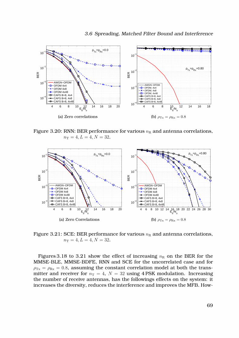
3.6 Spreading, Matched Filter Bound and Interference
4 6 8 10 12 14 16 18 20
10−4
10−3
10−2
10−1
Eb/N
o
BE
R
ρTx
=ρRx
=0.0
AWGN−OFDMOFDM 4x4OFDM 4x8OFDM 4x48CAFS B=8, 4x4CAFS B=8, 4x8CAFS B=8, 4x48
(a) Zero correlations
4 6 8 10 12 14 16 1810
−4
10−3
10−2
10−1
Eb/N
o
BE
R
ρTx
=ρRx
=0.80
AWGN−OFDMOFDM, 4x4OFDM, 4x8OFDM, 4x48CAFS B=8, 4x4CAFS B=8, 4x8CAFS B=8, 4x48
(b) ρTx = ρRx = 0.8
Figure 3.20: RNN: BER performance for various nR and antenna correlations,nT = 4, L = 4, N = 32.
4 6 8 10 12 14 16 18 20
10−4
10−3
10−2
10−1
Eb/N
o
BE
R
ρTx
=ρRx
=0.0
AWGN−OFDMOFDM 4x4OFDM 4x8OFDM 4x48CAFS B=8, 4x4CAFS B=8, 4x8CAFS B=8, 4x48
(a) Zero Correlations
4 6 8 10 12 14 16 18 20 22 24 26 28 30
10−4
10−3
10−2
10−1
Eb/N
o
BE
R
ρTx
=ρRx
=0.80
AWGN−OFDMOFDM 4x4OFDM 4x8OFDM 4x48CAFS B=8, 4x4CAFS B=8, 4x8CAFS B=8, 4x48
(b) ρTx = ρRx = 0.8
Figure 3.21: SCE: BER performance for various nR and antenna correlations,nT = 4, L = 4, N = 32.
Figures 3.18 to 3.21 show the effect of increasing nR on the BER for theMMSE-BLE, MMSE-BDFE, RNN and SCE for the uncorrelated case and forρTx = ρRx = 0.8, assuming the constant correlation model at both the trans-mitter and receiver for nT = 4, N = 32 using 4 PSK modulation. Increasingthe number of receive antennas, has the followings effects on the system: itincreases the diversity, reduces the interference and improves the MFB. How-
69
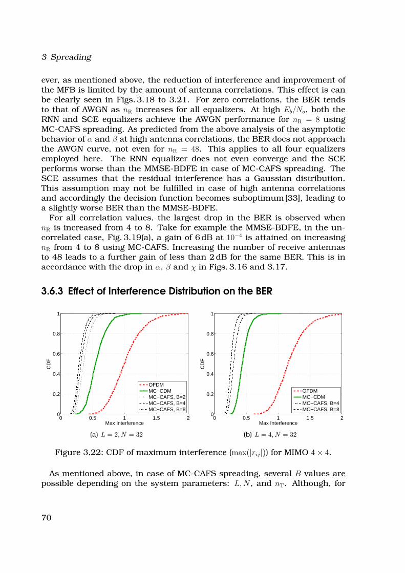
3 Spreading
ever, as mentioned above, the reduction of interference and improvement ofthe MFB is limited by the amount of antenna correlations. This effect is canbe clearly seen in Figs. 3.18 to 3.21. For zero correlations, the BER tendsto that of AWGN as nR increases for all equalizers. At high Eb/No, both theRNN and SCE equalizers achieve the AWGN performance for nR = 8 usingMC-CAFS spreading. As predicted from the above analysis of the asymptoticbehavior of α and β at high antenna correlations, the BER does not approachthe AWGN curve, not even for nR = 48. This applies to all four equalizersemployed here. The RNN equalizer does not even converge and the SCEperforms worse than the MMSE-BDFE in case of MC-CAFS spreading. TheSCE assumes that the residual interference has a Gaussian distribution.This assumption may not be fulfilled in case of high antenna correlationsand accordingly the decision function becomes suboptimum [33], leading toa slightly worse BER than the MMSE-BDFE.
For all correlation values, the largest drop in the BER is observed whennR is increased from 4 to 8. Take for example the MMSE-BDFE, in the un-correlated case, Fig. 3.19(a), a gain of 6 dB at 10−4 is attained on increasingnR from 4 to 8 using MC-CAFS. Increasing the number of receive antennasto 48 leads to a further gain of less than 2 dB for the same BER. This is inaccordance with the drop in α, β and χ in Figs. 3.16 and 3.17.
3.6.3 Effect of Interference Distribution on the BER
0 0.5 1 1.5 20
0.2
0.4
0.6
0.8
1
Max Interference
CD
F
OFDMMC−CDMMC−CAFS, B=2MC−CAFS, B=4MC−CAFS, B=8
(a) L = 2, N = 32
0 0.5 1 1.5 20
0.2
0.4
0.6
0.8
1
Max Interference
CD
F
OFDMMC−CDMMC−CAFS, B=4MC−CAFS, B=8
(b) L = 4, N = 32
Figure 3.22: CDF of maximum interference (max(|rij|)) for MIMO 4 × 4.
As mentioned above, in case of MC-CAFS spreading, several B values arepossible depending on the system parameters: L,N , and nT. Although, for
70
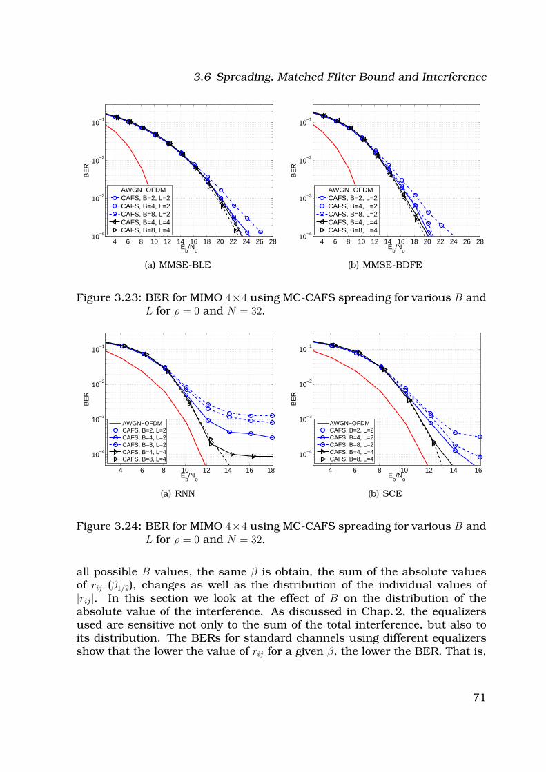
3.6 Spreading, Matched Filter Bound and Interference
4 6 8 10 12 14 16 18 20 22 24 26 2810
−4
10−3
10−2
10−1
Eb/N
o
BE
R
AWGN−OFDMCAFS, B=2, L=2CAFS, B=4, L=2CAFS, B=8, L=2CAFS, B=4, L=4CAFS, B=8, L=4
(a) MMSE-BLE
4 6 8 10 12 14 16 18 20 22 24 26 2810
−4
10−3
10−2
10−1
Eb/N
o
BE
R
AWGN−OFDMCAFS, B=2, L=2CAFS, B=4, L=2CAFS, B=8, L=2CAFS, B=4, L=4CAFS, B=8, L=4
(b) MMSE-BDFE
Figure 3.23: BER for MIMO 4×4 using MC-CAFS spreading for various B andL for ρ = 0 and N = 32.
4 6 8 10 12 14 16 18
10−4
10−3
10−2
10−1
Eb/N
o
BE
R
AWGN−OFDMCAFS, B=2, L=2CAFS, B=4, L=2CAFS, B=8, L=2CAFS, B=4, L=4CAFS, B=8, L=4
(a) RNN
4 6 8 10 12 14 16
10−4
10−3
10−2
10−1
Eb/N
o
BE
R
AWGN−OFDMCAFS, B=2, L=2CAFS, B=4, L=2CAFS, B=8, L=2CAFS, B=4, L=4CAFS, B=8, L=4
(b) SCE
Figure 3.24: BER for MIMO 4×4 using MC-CAFS spreading for various B andL for ρ = 0 and N = 32.
all possible B values, the same β is obtain, the sum of the absolute valuesof rij (β1/2), changes as well as the distribution of the individual values of|rij|. In this section we look at the effect of B on the distribution of theabsolute value of the interference. As discussed in Chap. 2, the equalizersused are sensitive not only to the sum of the total interference, but also toits distribution. The BERs for standard channels using different equalizersshow that the lower the value of rij for a given β, the lower the BER. That is,
71
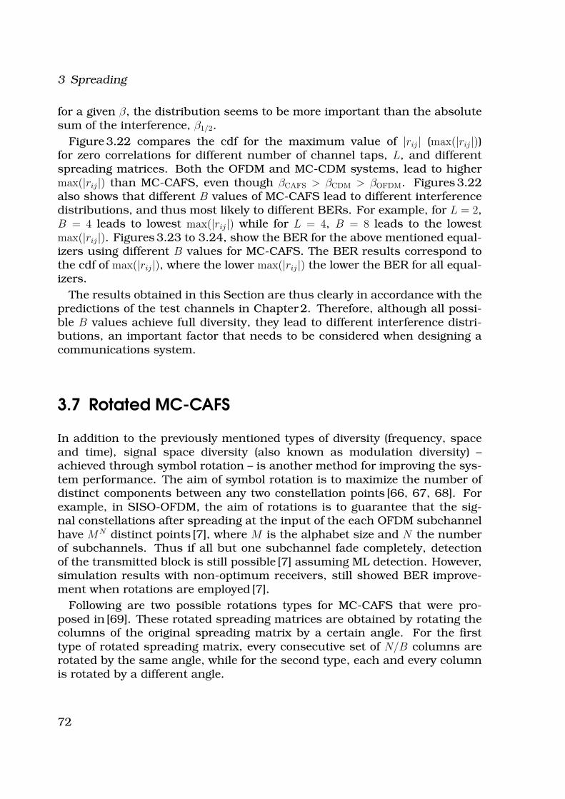
3 Spreading
for a given β, the distribution seems to be more important than the absolutesum of the interference, β1/2.
Figure 3.22 compares the cdf for the maximum value of |rij| (max(|rij|))for zero correlations for different number of channel taps, L, and differentspreading matrices. Both the OFDM and MC-CDM systems, lead to highermax(|rij|) than MC-CAFS, even though βCAFS > βCDM > βOFDM. Figures 3.22also shows that different B values of MC-CAFS lead to different interferencedistributions, and thus most likely to different BERs. For example, for L = 2,B = 4 leads to lowest max(|rij|) while for L = 4, B = 8 leads to the lowestmax(|rij|). Figures 3.23 to 3.24, show the BER for the above mentioned equal-izers using different B values for MC-CAFS. The BER results correspond tothe cdf of max(|rij|), where the lower max(|rij|) the lower the BER for all equal-izers.
The results obtained in this Section are thus clearly in accordance with thepredictions of the test channels in Chapter 2. Therefore, although all possi-ble B values achieve full diversity, they lead to different interference distri-butions, an important factor that needs to be considered when designing acommunications system.
3.7 Rotated MC-CAFS
In addition to the previously mentioned types of diversity (frequency, spaceand time), signal space diversity (also known as modulation diversity) –achieved through symbol rotation – is another method for improving the sys-tem performance. The aim of symbol rotation is to maximize the number ofdistinct components between any two constellation points [66, 67, 68]. Forexample, in SISO-OFDM, the aim of rotations is to guarantee that the sig-nal constellations after spreading at the input of the each OFDM subchannelhave MN distinct points [7], where M is the alphabet size and N the numberof subchannels. Thus if all but one subchannel fade completely, detectionof the transmitted block is still possible [7] assuming ML detection. However,simulation results with non-optimum receivers, still showed BER improve-ment when rotations are employed [7].
Following are two possible rotations types for MC-CAFS that were pro-posed in [69]. These rotated spreading matrices are obtained by rotating thecolumns of the original spreading matrix by a certain angle. For the firsttype of rotated spreading matrix, every consecutive set of N/B columns arerotated by the same angle, while for the second type, each and every columnis rotated by a different angle.
72

3.7 Rotated MC-CAFS
3.7.1 Rotations Type I
To obtain UMC−CAFSRotI
, the orthogonal matrix, S, in Sec. 3.5 used for calcu-
lating the spreading matrix UMC−CAFS
is replaced by SRot
which is given as
follows:S
Rot= S D
n, (3.50)
where Dn
is diagonal matrix of size n×n. The diagonal elements, dii, of Dn
forM-PSK are given by [7, 70]
dii = exp(
j2π
M
(i − 1)
n
)
, (3.51)
where i = 1, . . . , n and for rotations of Type I, n = nTB, the size of S. Thus,each column of S is rotated by a different angle or equivalently every N/Bconsecutive columns of U
MC−CAFSare rotated by the same angle. The rotated
spreading matrix, UMC−CAFSRotI
, can alternatively be obtained as follows,
UMC−CAFSRotI
= UMC−CAFS
DkronI
(3.52)
whereD
kronI= D
nTB⊗ I
N/B, (3.53)
and ⊗ is the Kronecker product, IN/B
is the identity matrix of size N/B ×N/B
and DnTB
is again given by Eqn. 3.51 with n = nTB.
3.7.2 Rotations Type II
To obtain UMC−CAFSRotII
, the spreading matrix UMC−CAFS
is postmultiplied by
the diagonal rotation matrix Dn
as follows:
UMC−CAFSRotII
= UMC−CAFS
Dn
(3.54)
Again, Dn
is a diagonal matrix whose diagonal elements are given byEqn. 3.51. However, n = nTN in this case. Thus, for rotations type II, allantennas and frequencies are rotated by different angles.
Assessment of Rotated MC-CAFS
To assess how rotations can affect the system performance, we shall look atthe following three aspects:
- the minimum Euclidean distance after the channel,
73
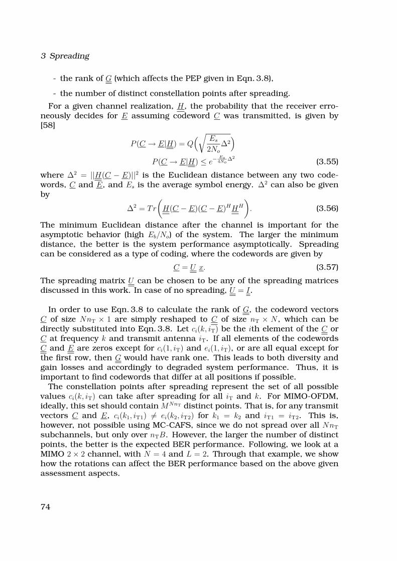
3 Spreading
- the rank of G (which affects the PEP given in Eqn. 3.8),
- the number of distinct constellation points after spreading.
For a given channel realization, H, the probability that the receiver erro-neously decides for E assuming codeword C was transmitted, is given by[58]
P (C → E|H) = Q(
√
Es
2No
∆2)
P (C → E|H) ≤ e−Es4No
∆2
(3.55)
where ∆2 = ||H(C − E)||2 is the Euclidean distance between any two code-words, C and E, and Es is the average symbol energy. ∆2 can also be givenby
∆2 = Tr
(
H(C − E)(C − E)HHH
)
. (3.56)
The minimum Euclidean distance after the channel is important for theasymptotic behavior (high Eb/No) of the system. The larger the minimumdistance, the better is the system performance asymptotically. Spreadingcan be considered as a type of coding, where the codewords are given by
C = U x. (3.57)
The spreading matrix U can be chosen to be any of the spreading matricesdiscussed in this work. In case of no spreading, U = I.
In order to use Eqn. 3.8 to calculate the rank of G, the codeword vectorsC of size NnT × 1 are simply reshaped to C of size nT × N , which can bedirectly substituted into Eqn. 3.8. Let ci(k, iT) be the ith element of the C orC at frequency k and transmit antenna iT. If all elements of the codewordsC and E are zeros except for ci(1, iT) and ei(1, iT), or are all equal except forthe first row, then G would have rank one. This leads to both diversity andgain losses and accordingly to degraded system performance. Thus, it isimportant to find codewords that differ at all positions if possible.
The constellation points after spreading represent the set of all possiblevalues ci(k, iT) can take after spreading for all iT and k. For MIMO-OFDM,ideally, this set should contain MNnT distinct points. That is, for any transmitvectors C and E, ci(k1, iT1) 6= ei(k2, iT2) for k1 = k2 and iT1 = iT2. This is,however, not possible using MC-CAFS, since we do not spread over all NnT
subchannels, but only over nTB. However, the larger the number of distinctpoints, the better is the expected BER performance. Following, we look at aMIMO 2 × 2 channel, with N = 4 and L = 2. Through that example, we showhow the rotations can affect the BER performance based on the above givenassessment aspects.
74
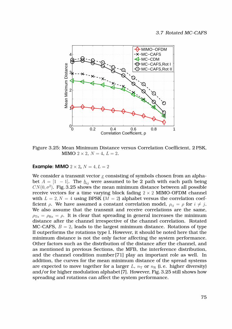
3.7 Rotated MC-CAFS
0 0.2 0.4 0.6 0.8 10
1
2
3
4
Correlation Coefficient, ρ
Mea
n M
inim
um D
ista
nce
MIMO−OFDMMC−CAFSMC−CDMMC−CAFS,Rot IMC−CAFS,Rot II
Figure 3.25: Mean Minimum Distance versus Correlation Coefficient, 2 PSK,MIMO 2 × 2, N = 4, L = 2.
Example: MIMO 2 × 2, N = 4, L = 2
We consider a transmit vector x consisting of symbols chosen from an alpha-bet A = [1 − 1]. The hij were assumed to be 2 path with each path beingCN(0, σ2). Fig. 3.25 shows the mean minimum distance between all possiblereceive vectors for a time varying block fading 2 × 2 MIMO-OFDM channelwith L = 2, N = 4 using BPSK (M = 2) alphabet versus the correlation coef-ficient ρ. We have assumed a constant correlation model, ρij = ρ for i 6= j.We also assume that the transmit and receive correlations are the same,ρTx = ρRx = ρ. It is clear that spreading in general increases the minimumdistance after the channel irrespective of the channel correlation. RotatedMC-CAFS, B = 2, leads to the largest minimum distance. Rotations of typeII outperforms the rotations type I. However, it should be noted here that theminimum distance is not the only factor affecting the system performance.Other factors such as the distribution of the distance after the channel, andas mentioned in previous Sections, the MFB, the interference distribution,and the channel condition number [71] play an important role as well. Inaddition, the curves for the mean minimum distance of the spread systemsare expected to move together for a larger L, nT or nR (i. e. higher diversity)and/or for higher modulation alphabet [7]. However, Fig. 3.25 still shows howspreading and rotations can affect the system performance.
75
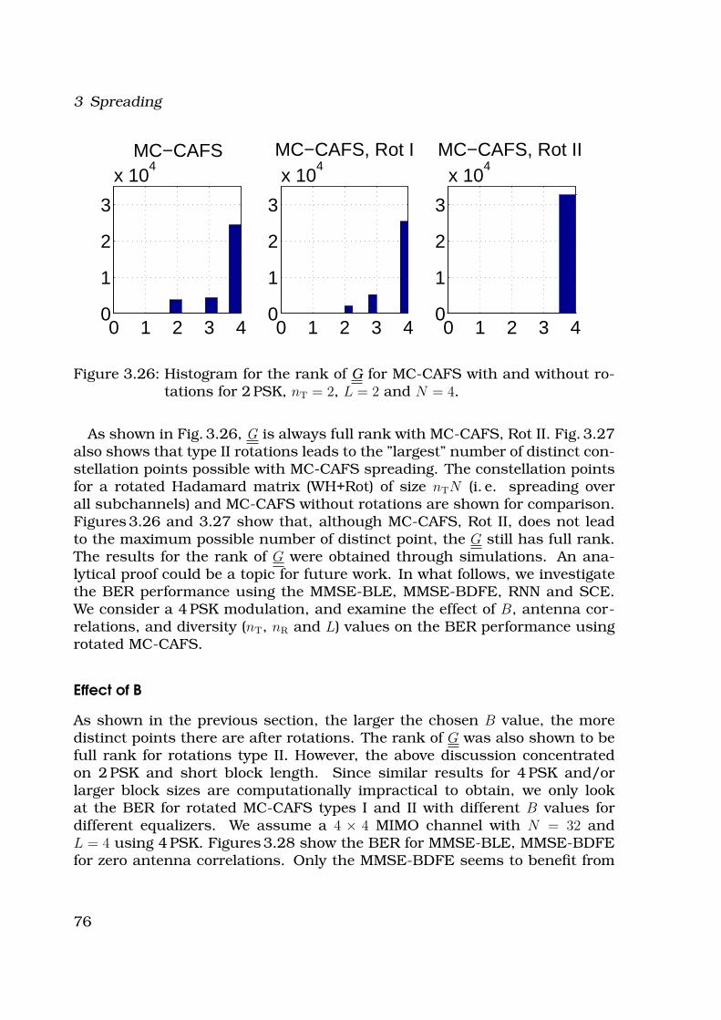
3 Spreading
0 1 2 3 40
1
2
3
x 104
MC−CAFS
0 1 2 3 40
1
2
3
x 104
MC−CAFS, Rot I
0 1 2 3 40
1
2
3
x 104
MC−CAFS, Rot II
Figure 3.26: Histogram for the rank of G for MC-CAFS with and without ro-tations for 2 PSK, nT = 2, L = 2 and N = 4.
As shown in Fig. 3.26, G is always full rank with MC-CAFS, Rot II. Fig. 3.27also shows that type II rotations leads to the ”largest” number of distinct con-stellation points possible with MC-CAFS spreading. The constellation pointsfor a rotated Hadamard matrix (WH+Rot) of size nTN (i. e. spreading overall subchannels) and MC-CAFS without rotations are shown for comparison.Figures 3.26 and 3.27 show that, although MC-CAFS, Rot II, does not leadto the maximum possible number of distinct point, the G still has full rank.The results for the rank of G were obtained through simulations. An ana-lytical proof could be a topic for future work. In what follows, we investigatethe BER performance using the MMSE-BLE, MMSE-BDFE, RNN and SCE.We consider a 4 PSK modulation, and examine the effect of B, antenna cor-relations, and diversity (nT, nR and L) values on the BER performance usingrotated MC-CAFS.
Effect of B
As shown in the previous section, the larger the chosen B value, the moredistinct points there are after rotations. The rank of G was also shown to befull rank for rotations type II. However, the above discussion concentratedon 2 PSK and short block length. Since similar results for 4 PSK and/orlarger block sizes are computationally impractical to obtain, we only lookat the BER for rotated MC-CAFS types I and II with different B values fordifferent equalizers. We assume a 4 × 4 MIMO channel with N = 32 andL = 4 using 4 PSK. Figures 3.28 show the BER for MMSE-BLE, MMSE-BDFEfor zero antenna correlations. Only the MMSE-BDFE seems to benefit from
76
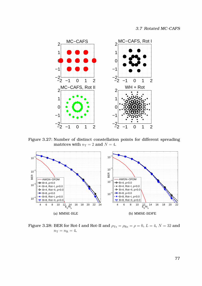
3.7 Rotated MC-CAFS
−2 −1 0 1 2−2
−1
0
1
2MC−CAFS, Rot I
−2 −1 0 1 2−2
−1
0
1
2MC−CAFS, Rot II
−2 −1 0 1 2−2
−1
0
1
2MC−CAFS
−2 −1 0 1 2−2
−1
0
1
2WH + Rot
Figure 3.27: Number of distinct constellation points for different spreadingmatrices with nT = 2 and N = 4.
4 6 8 10 12 14 16 18 20 22 24
10−4
10−3
10−2
10−1
Eb/N
o
BE
R
AWGN−OFDMB=4, ρ=0.0B=4, Rot−I, ρ=0.0B=4, Rot−II, ρ=0.0B=8, ρ=0.0B=8, Rot−I, ρ=0.0B=8, Rot−II, ρ=0.0
(a) MMSE-BLE
4 6 8 10 12 14 16 18 20 22
10−4
10−3
10−2
10−1
Eb/N
o
BE
R
AWGN−OFDMB=4, ρ=0.0B=4, Rot−I, ρ=0.0B=4, Rot−II, ρ=0.0B=8, ρ=0.0B=8, Rot−I, ρ=0.0B=8, Rot−II, ρ=0.0
(b) MMSE-BDFE
Figure 3.28: BER for Rot-I and Rot-II and ρTx = ρRx = ρ = 0, L = 4, N = 32 andnT = nR = 4.
77
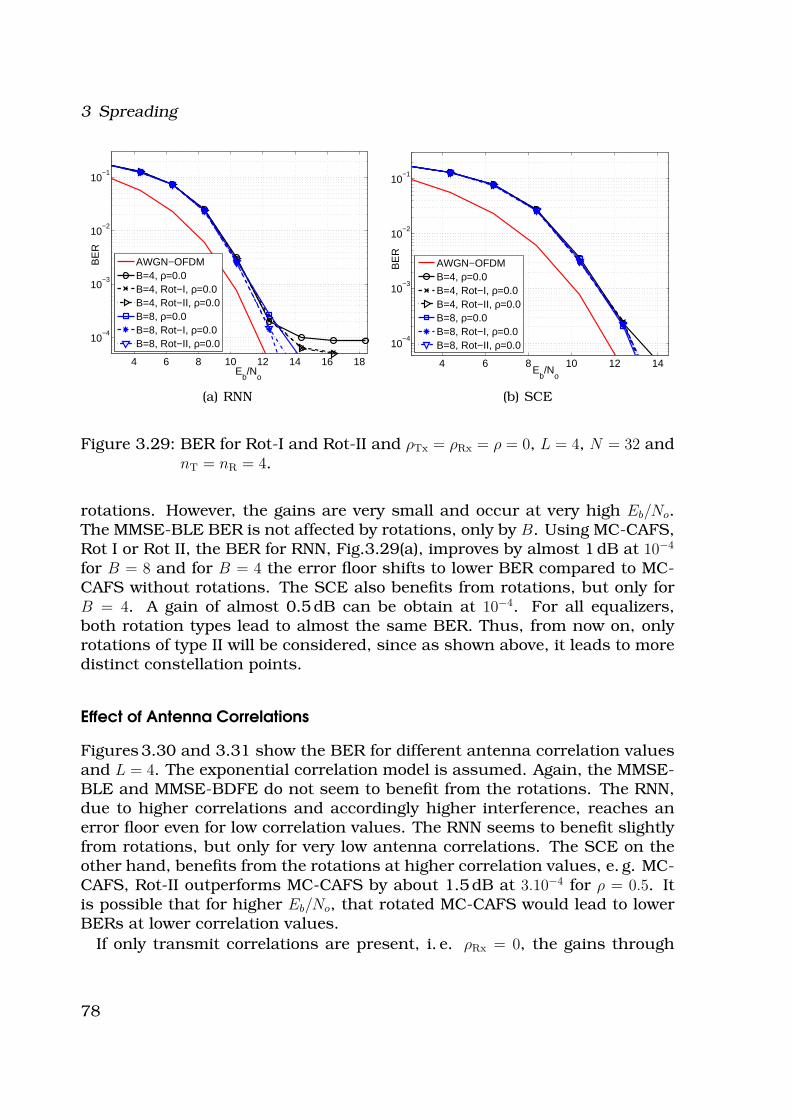
3 Spreading
4 6 8 10 12 14 16 18
10−4
10−3
10−2
10−1
Eb/N
o
BE
R
AWGN−OFDMB=4, ρ=0.0B=4, Rot−I, ρ=0.0B=4, Rot−II, ρ=0.0B=8, ρ=0.0B=8, Rot−I, ρ=0.0B=8, Rot−II, ρ=0.0
(a) RNN
4 6 8 10 12 14
10−4
10−3
10−2
10−1
Eb/N
o
BE
R
AWGN−OFDMB=4, ρ=0.0B=4, Rot−I, ρ=0.0B=4, Rot−II, ρ=0.0B=8, ρ=0.0B=8, Rot−I, ρ=0.0B=8, Rot−II, ρ=0.0
(b) SCE
Figure 3.29: BER for Rot-I and Rot-II and ρTx = ρRx = ρ = 0, L = 4, N = 32 andnT = nR = 4.
rotations. However, the gains are very small and occur at very high Eb/No.The MMSE-BLE BER is not affected by rotations, only by B. Using MC-CAFS,Rot I or Rot II, the BER for RNN, Fig.3.29(a), improves by almost 1 dB at 10−4
for B = 8 and for B = 4 the error floor shifts to lower BER compared to MC-CAFS without rotations. The SCE also benefits from rotations, but only forB = 4. A gain of almost 0.5 dB can be obtain at 10−4. For all equalizers,both rotation types lead to almost the same BER. Thus, from now on, onlyrotations of type II will be considered, since as shown above, it leads to moredistinct constellation points.
Effect of Antenna Correlations
Figures 3.30 and 3.31 show the BER for different antenna correlation valuesand L = 4. The exponential correlation model is assumed. Again, the MMSE-BLE and MMSE-BDFE do not seem to benefit from the rotations. The RNN,due to higher correlations and accordingly higher interference, reaches anerror floor even for low correlation values. The RNN seems to benefit slightlyfrom rotations, but only for very low antenna correlations. The SCE on theother hand, benefits from the rotations at higher correlation values, e. g. MC-CAFS, Rot-II outperforms MC-CAFS by about 1.5 dB at 3.10−4 for ρ = 0.5. Itis possible that for higher Eb/No, that rotated MC-CAFS would lead to lowerBERs at lower correlation values.
If only transmit correlations are present, i. e. ρRx = 0, the gains through
78
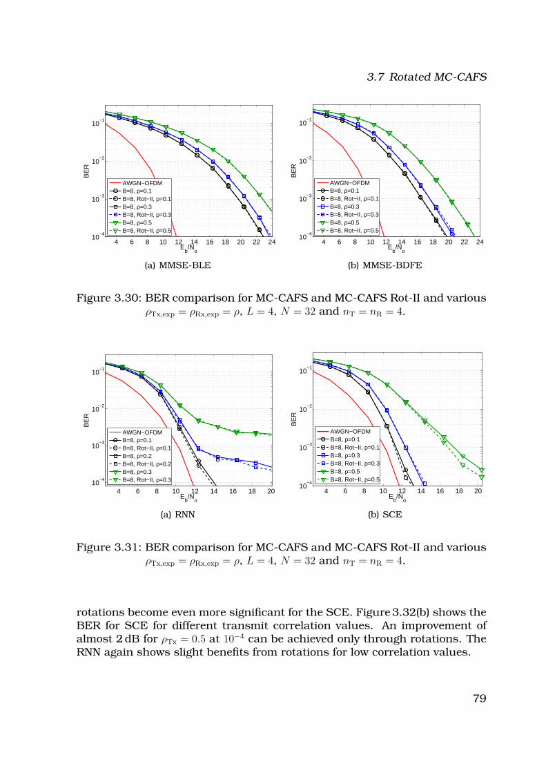
3.7 Rotated MC-CAFS
4 6 8 10 12 14 16 18 20 22 2410
−4
10−3
10−2
10−1
Eb/N
o
BE
R
AWGN−OFDMB=8, ρ=0.1B=8, Rot−II, ρ=0.1B=8, ρ=0.3B=8, Rot−II, ρ=0.3B=8, ρ=0.5B=8, Rot−II, ρ=0.5
(a) MMSE-BLE
4 6 8 10 12 14 16 18 20 22 2410
−4
10−3
10−2
10−1
Eb/N
o
BE
R
AWGN−OFDMB=8, ρ=0.1B=8, Rot−II, ρ=0.1B=8, ρ=0.3B=8, Rot−II, ρ=0.3B=8, ρ=0.5B=8, Rot−II, ρ=0.5
(b) MMSE-BDFE
Figure 3.30: BER comparison for MC-CAFS and MC-CAFS Rot-II and variousρTx,exp = ρRx,exp = ρ, L = 4, N = 32 and nT = nR = 4.
4 6 8 10 12 14 16 18 2010
−4
10−3
10−2
10−1
Eb/N
o
BE
R
AWGN−OFDMB=8, ρ=0.1B=8, Rot−II, ρ=0.1B=8, ρ=0.2B=8, Rot−II, ρ=0.2B=8, ρ=0.3B=8, Rot−II, ρ=0.3
(a) RNN
4 6 8 10 12 14 16 18 2010
−4
10−3
10−2
10−1
Eb/N
o
BE
R
AWGN−OFDMB=8, ρ=0.1B=8, Rot−II, ρ=0.1B=8, ρ=0.3B=8, Rot−II, ρ=0.3B=8, ρ=0.5B=8, Rot−II, ρ=0.5
(b) SCE
Figure 3.31: BER comparison for MC-CAFS and MC-CAFS Rot-II and variousρTx,exp = ρRx,exp = ρ, L = 4, N = 32 and nT = nR = 4.
rotations become even more significant for the SCE. Figure 3.32(b) shows theBER for SCE for different transmit correlation values. An improvement ofalmost 2 dB for ρTx = 0.5 at 10−4 can be achieved only through rotations. TheRNN again shows slight benefits from rotations for low correlation values.
79
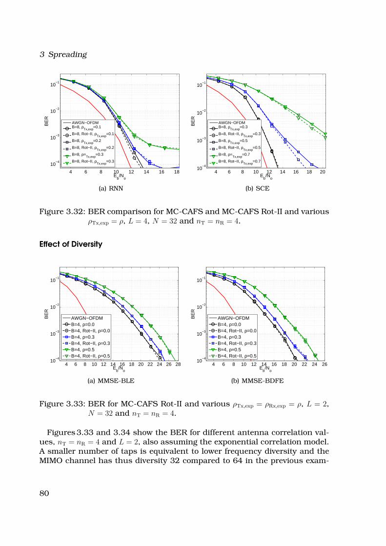
3 Spreading
4 6 8 10 12 14 16 18
10−4
10−3
10−2
10−1
Eb/N
o
BE
R
AWGN−OFDMB=8, ρ
Tx,exp=0.1
B=8, Rot−II, ρTx,exp
=0.1
B=8, ρTx,exp
=0.2
B=8, Rot−II, ρTx,exp
=0.2
B=8, ρ=Tx,exp
=0.3
B=8, Rot−II, ρTx,exp
=0.3
(a) RNN
4 6 8 10 12 14 16 18 2010
−4
10−3
10−2
10−1
Eb/N
o
BE
R
AWGN−OFDMB=8, ρ
Tx,exp=0.3
B=8, Rot−II, ρTx,exp
=0.3
B=8, ρTx,exp
=0.5
B=8, Rot−II, ρTx,exp
=0.5
B=8, ρ=Tx,exp
=0.7
B=8, Rot−II, ρTx,exp
=0.7
(b) SCE
Figure 3.32: BER comparison for MC-CAFS and MC-CAFS Rot-II and variousρTx,exp = ρ, L = 4, N = 32 and nT = nR = 4.
Effect of Diversity
4 6 8 10 12 14 16 18 20 22 24 26 2810
−4
10−3
10−2
10−1
Eb/N
o
BE
R
AWGN−OFDMB=4, ρ=0.0B=4, Rot−II, ρ=0.0B=4, ρ=0.3B=4, Rot−II, ρ=0.3B=4, ρ=0.5B=4, Rot−II, ρ=0.5
(a) MMSE-BLE
4 6 8 10 12 14 16 18 20 22 24 2610
−4
10−3
10−2
10−1
Eb/N
o
BE
R
AWGN−OFDMB=4, ρ=0.0B=4, Rot−II, ρ=0.0B=4, ρ=0.3B=4, Rot−II, ρ=0.3B=4, ρ=0.5B=4, Rot−II, ρ=0.5
(b) MMSE-BDFE
Figure 3.33: BER for MC-CAFS Rot-II and various ρTx,exp = ρRx,exp = ρ, L = 2,N = 32 and nT = nR = 4.
Figures 3.33 and 3.34 show the BER for different antenna correlation val-ues, nT = nR = 4 and L = 2, also assuming the exponential correlation model.A smaller number of taps is equivalent to lower frequency diversity and theMIMO channel has thus diversity 32 compared to 64 in the previous exam-
80
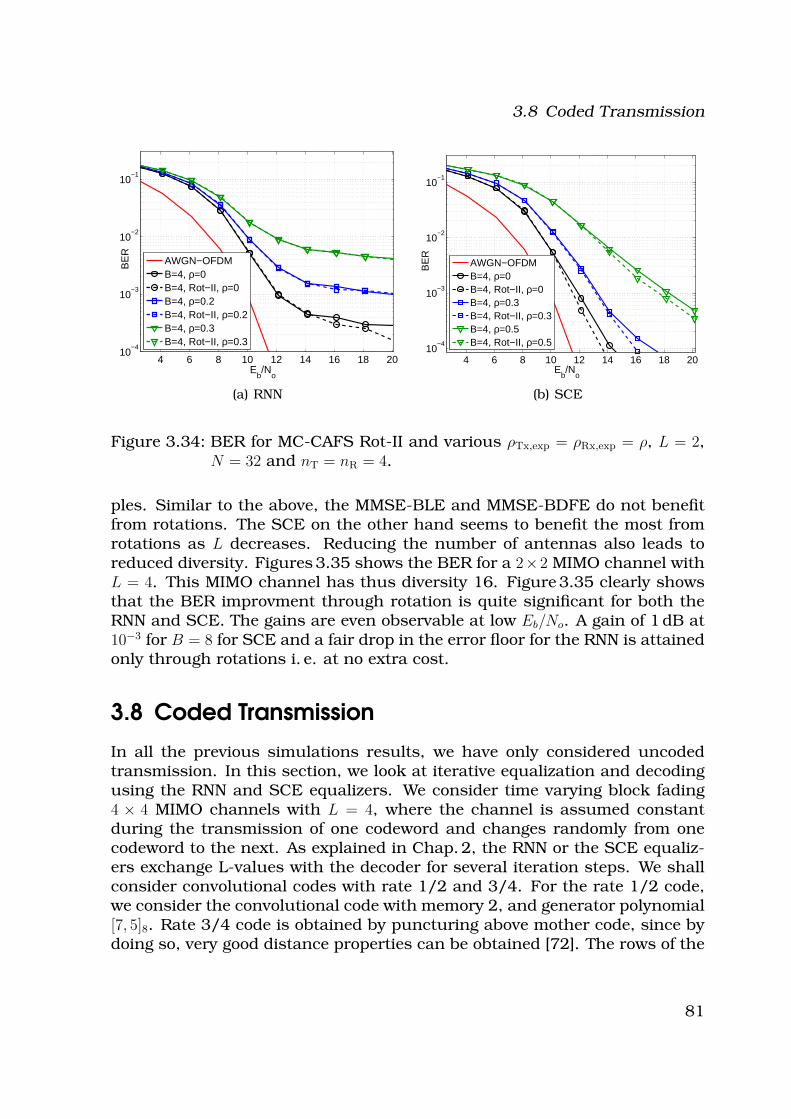
3.8 Coded Transmission
4 6 8 10 12 14 16 18 2010
−4
10−3
10−2
10−1
Eb/N
o
BE
R
AWGN−OFDMB=4, ρ=0B=4, Rot−II, ρ=0B=4, ρ=0.2B=4, Rot−II, ρ=0.2B=4, ρ=0.3B=4, Rot−II, ρ=0.3
(a) RNN
4 6 8 10 12 14 16 18 2010
−4
10−3
10−2
10−1
Eb/N
o
BE
R
AWGN−OFDMB=4, ρ=0B=4, Rot−II, ρ=0B=4, ρ=0.3B=4, Rot−II, ρ=0.3B=4, ρ=0.5B=4, Rot−II, ρ=0.5
(b) SCE
Figure 3.34: BER for MC-CAFS Rot-II and various ρTx,exp = ρRx,exp = ρ, L = 2,N = 32 and nT = nR = 4.
ples. Similar to the above, the MMSE-BLE and MMSE-BDFE do not benefitfrom rotations. The SCE on the other hand seems to benefit the most fromrotations as L decreases. Reducing the number of antennas also leads toreduced diversity. Figures 3.35 shows the BER for a 2×2 MIMO channel withL = 4. This MIMO channel has thus diversity 16. Figure 3.35 clearly showsthat the BER improvment through rotation is quite significant for both theRNN and SCE. The gains are even observable at low Eb/No. A gain of 1 dB at10−3 for B = 8 for SCE and a fair drop in the error floor for the RNN is attainedonly through rotations i. e. at no extra cost.
3.8 Coded Transmission
In all the previous simulations results, we have only considered uncodedtransmission. In this section, we look at iterative equalization and decodingusing the RNN and SCE equalizers. We consider time varying block fading4 × 4 MIMO channels with L = 4, where the channel is assumed constantduring the transmission of one codeword and changes randomly from onecodeword to the next. As explained in Chap. 2, the RNN or the SCE equaliz-ers exchange L-values with the decoder for several iteration steps. We shallconsider convolutional codes with rate 1/2 and 3/4. For the rate 1/2 code,we consider the convolutional code with memory 2, and generator polynomial[7, 5]8. Rate 3/4 code is obtained by puncturing above mother code, since bydoing so, very good distance properties can be obtained [72]. The rows of the
81
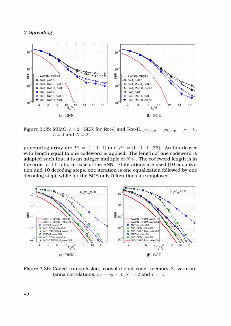
3 Spreading
4 6 8 10 12 14 16 1810
−4
10−3
10−2
10−1
Eb/N
o
BE
R
AWGN−OFDMB=4, ρ=0.0B=4, Rot−I, ρ=0.0B=4, Rot−II, ρ=0.0B=8, ρ=0.0B=8, Rot−I, ρ=0.0B=8, Rot−II, ρ=0.0
(a) RNN
4 6 8 10 12 14 1610
−4
10−3
10−2
10−1
Eb/N
o
BE
R
AWGN−OFDMB=4, ρ=0.0B=4, Rot−I, ρ=0.0B=4, Rot−II, ρ=0.0B=8, ρ=0.0B=8, Rot−I, ρ=0.0B=8, Rot−II, ρ=0.0
(b) SCE
Figure 3.35: MIMO 2 × 2: BER for Rot-I and Rot-II, ρTx,exp = ρRx,exp = ρ = 0,L = 4 and N = 32.
puncturing array are P1 = [1 0 1] and P2 = [1 1 0] [73]. An interleaverwith length equal to one codeword is applied. The length of one codeword isadapted such that it is an integer multiple of NnT. The codeword length is inthe order of 104 bits. In case of the RNN, 10 iterations are used (10 equaliza-tion and 10 decoding steps, one iteration is one equalization followed by onedecoding step), while for the SCE only 5 iterations are employed.
4 5 6 7 8 9 10 11
10−5
10−4
10−3
10−2
10−1
Eb/N
o
BE
R
ρTx
=ρRx
=0.0
AWGN−OFDM, rate=1/2AWGN−OFDM, rate=3/4OFDM, rate=1/2MC−CDM, rate=1/2MC−CAFS B=4, rate=1/2OFDM, rate=3/4MC−CDM, rate=3/4MC−CAFS B=4, rate=3/4
(a) RNN
4 5 6 7 8 9 10 11
10−5
10−4
10−3
10−2
10−1
Eb/N
o
BE
R
ρTx
=ρRx
=0.0
AWGN−OFDM, rate=1/2AWGN−OFDM, rate=3/4OFDM, rate=1/2MC−CDM, rate=1/2MC−CAFS B=4, rate=1/2OFDM, rate=3/4MC−CDM, rate=3/4MC−CAFS B=4, rate=3/4
(b) SCE
Figure 3.36: Coded transmission, convolutional code, memory 2, zero an-tenna correlations, nT = nR = 4, N = 32 and L = 4.
82
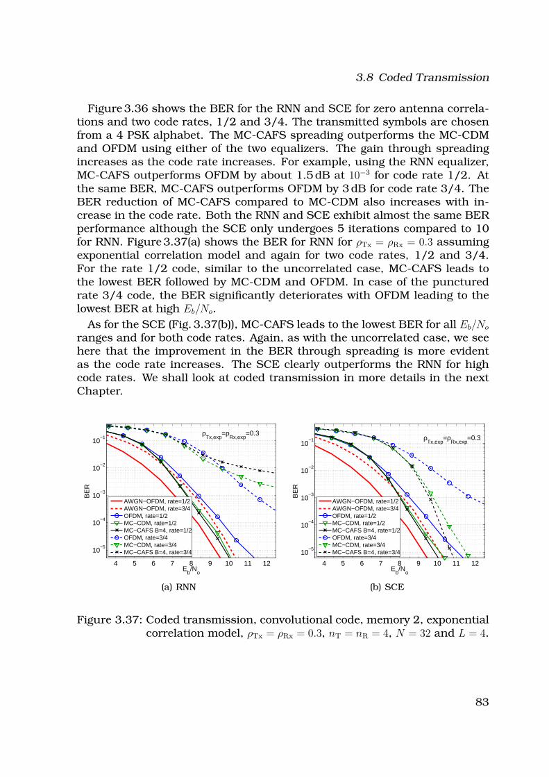
3.8 Coded Transmission
Figure 3.36 shows the BER for the RNN and SCE for zero antenna correla-tions and two code rates, 1/2 and 3/4. The transmitted symbols are chosenfrom a 4 PSK alphabet. The MC-CAFS spreading outperforms the MC-CDMand OFDM using either of the two equalizers. The gain through spreadingincreases as the code rate increases. For example, using the RNN equalizer,MC-CAFS outperforms OFDM by about 1.5 dB at 10−3 for code rate 1/2. Atthe same BER, MC-CAFS outperforms OFDM by 3 dB for code rate 3/4. TheBER reduction of MC-CAFS compared to MC-CDM also increases with in-crease in the code rate. Both the RNN and SCE exhibit almost the same BERperformance although the SCE only undergoes 5 iterations compared to 10for RNN. Figure 3.37(a) shows the BER for RNN for ρTx = ρRx = 0.3 assumingexponential correlation model and again for two code rates, 1/2 and 3/4.For the rate 1/2 code, similar to the uncorrelated case, MC-CAFS leads tothe lowest BER followed by MC-CDM and OFDM. In case of the puncturedrate 3/4 code, the BER significantly deteriorates with OFDM leading to thelowest BER at high Eb/No.
As for the SCE (Fig. 3.37(b)), MC-CAFS leads to the lowest BER for all Eb/No
ranges and for both code rates. Again, as with the uncorrelated case, we seehere that the improvement in the BER through spreading is more evidentas the code rate increases. The SCE clearly outperforms the RNN for highcode rates. We shall look at coded transmission in more details in the nextChapter.
4 5 6 7 8 9 10 11 12
10−5
10−4
10−3
10−2
10−1
Eb/N
o
BE
R
ρTx,exp
=ρRx,exp
=0.3
AWGN−OFDM, rate=1/2AWGN−OFDM, rate=3/4OFDM, rate=1/2MC−CDM, rate=1/2MC−CAFS B=4, rate=1/2OFDM, rate=3/4MC−CDM, rate=3/4MC−CAFS B=4, rate=3/4
(a) RNN
4 5 6 7 8 9 10 11 12
10−5
10−4
10−3
10−2
10−1
Eb/N
o
BE
R
ρTx,exp
=ρRx,exp
=0.3
AWGN−OFDM, rate=1/2AWGN−OFDM, rate=3/4OFDM, rate=1/2MC−CDM, rate=1/2MC−CAFS B=4, rate=1/2OFDM, rate=3/4MC−CDM, rate=3/4MC−CAFS B=4, rate=3/4
(b) SCE
Figure 3.37: Coded transmission, convolutional code, memory 2, exponentialcorrelation model, ρTx = ρRx = 0.3, nT = nR = 4, N = 32 and L = 4.
83
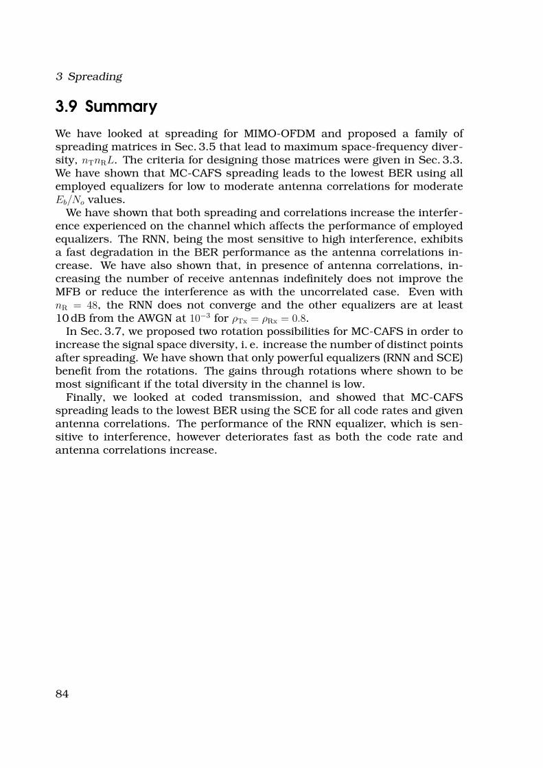
3 Spreading
3.9 Summary
We have looked at spreading for MIMO-OFDM and proposed a family ofspreading matrices in Sec. 3.5 that lead to maximum space-frequency diver-sity, nTnRL. The criteria for designing those matrices were given in Sec. 3.3.We have shown that MC-CAFS spreading leads to the lowest BER using allemployed equalizers for low to moderate antenna correlations for moderateEb/No values.
We have shown that both spreading and correlations increase the interfer-ence experienced on the channel which affects the performance of employedequalizers. The RNN, being the most sensitive to high interference, exhibitsa fast degradation in the BER performance as the antenna correlations in-crease. We have also shown that, in presence of antenna correlations, in-creasing the number of receive antennas indefinitely does not improve theMFB or reduce the interference as with the uncorrelated case. Even withnR = 48, the RNN does not converge and the other equalizers are at least10 dB from the AWGN at 10−3 for ρTx = ρRx = 0.8.
In Sec. 3.7, we proposed two rotation possibilities for MC-CAFS in order toincrease the signal space diversity, i. e. increase the number of distinct pointsafter spreading. We have shown that only powerful equalizers (RNN and SCE)benefit from the rotations. The gains through rotations where shown to bemost significant if the total diversity in the channel is low.
Finally, we looked at coded transmission, and showed that MC-CAFSspreading leads to the lowest BER using the SCE for all code rates and givenantenna correlations. The performance of the RNN equalizer, which is sen-sitive to interference, however deteriorates fast as both the code rate andantenna correlations increase.
84
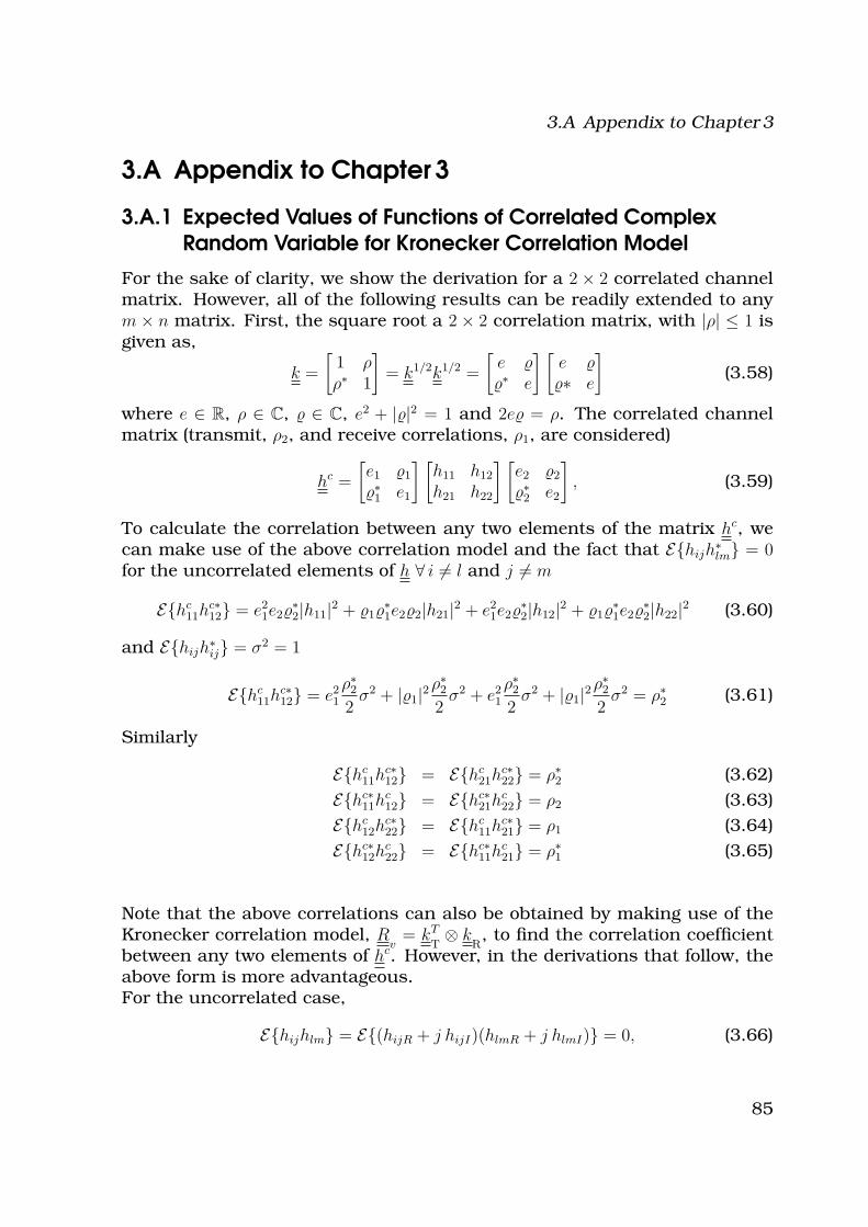
3.A Appendix to Chapter 3
3.A Appendix to Chapter 3
3.A.1 Expected Values of Functions of Correlated Complex
Random Variable for Kronecker Correlation Model
For the sake of clarity, we show the derivation for a 2 × 2 correlated channelmatrix. However, all of the following results can be readily extended to anym × n matrix. First, the square root a 2 × 2 correlation matrix, with |ρ| ≤ 1 isgiven as,
k =
[
1 ρρ∗ 1
]
= k1/2k1/2 =
[
e ∗ e
] [
e ∗ e
]
(3.58)
where e ∈ R, ρ ∈ C, ∈ C, e2 + ||2 = 1 and 2e = ρ. The correlated channelmatrix (transmit, ρ2, and receive correlations, ρ1, are considered)
hc =
[
e1 1
∗1 e1
] [
h11 h12
h21 h22
] [
e2 2
∗2 e2
]
, (3.59)
To calculate the correlation between any two elements of the matrix hc, wecan make use of the above correlation model and the fact that E{hijh
∗lm} = 0
for the uncorrelated elements of h ∀ i 6= l and j 6= m
E{hc11h
c∗12} = e2
1e2∗2|h11|2 + 1
∗1e22|h21|2 + e2
1e2∗2|h12|2 + 1
∗1e2
∗2|h22|2 (3.60)
and E{hijh∗ij} = σ2 = 1
E{hc11h
c∗12} = e2
1
ρ∗2
2σ2 + |1|2
ρ∗2
2σ2 + e2
1
ρ∗2
2σ2 + |1|2
ρ∗2
2σ2 = ρ∗
2 (3.61)
Similarly
E{hc11h
c∗12} = E{hc
21hc∗22} = ρ∗
2 (3.62)
E{hc∗11h
c12} = E{hc∗
21hc22} = ρ2 (3.63)
E{hc12h
c∗22} = E{hc
11hc∗21} = ρ1 (3.64)
E{hc∗12h
c22} = E{hc∗
11hc21} = ρ∗
1 (3.65)
Note that the above correlations can also be obtained by making use of theKronecker correlation model, R
v= kT
T⊗ k
R, to find the correlation coefficient
between any two elements of hc. However, in the derivations that follow, theabove form is more advantageous.For the uncorrelated case,
E{hijhlm} = E{(hijR + j hijI)(hlmR + j hlmI)} = 0, (3.66)
85
3 Spreading
since the real and imaginary parts are assumed independent. FromEqn. 3.66, It can be shown that for σ2
real = σ2imag = σ2/2
E{hijhij} = σ2real − σ2
imag = 0, (3.67)
Using the correlation model of Eqn. 3.59, the results of Eqns. 3.66, 3.67, andproceeding with the derivation as in Eqn. 3.60, it can be shown that
E{hcijh
clm} = 0, (3.68)
∀ i, j, l and m. Using Eqns. 3.66 to 3.68, we now can derive the expectedvalues of functions of the correlated complex random variables.If xi are real jointly normal random variables with mean zero, variance one,and E{xixj} = ρij, then [43]
E{x1x2x3x4} = ρ12ρ34 + ρ13ρ24 + ρ14ρ23 (3.69)
For complex random variables xi (CN(0, 1)), Eqn. 3.70 can be derived by ex-panding xi into their real and imaginary parts and using Eqns. 3.67, 3.68and 3.69.
E{x∗1x2x3x
∗4} = ρ∗
12ρ34 + ρ∗13ρ24 (3.70)
For any two real random variables, x and y, that are jointly normal with zeromean [43]
E{x2y2} = E{x2}E{y2} + 2E2{xy} (3.71)
Accordingly, for two CN(0, 1) random variables, x and y, the following Eqn.can be derived
E{|x|2|y|2}=E{(x2real + x2
imag)(y2real + y2
imag)}=1 + |ρxy|2 (3.72)
From Eqn. 3.72,E{|x|4} = E{|x|2|x|2} = 2, (3.73)
since |ρxx|2 = 1.
86
3.A Appendix to Chapter 3
3.A.2 Expected values of α, β and the var(r)
The aim of the following derivations is to find a closed form expression forthe E{α} and E{β} as a function the antenna correlations and the numberof transmit and receive antennas for the unspread MIMO-OFDM system. Inall that follows, we assume that HiRiT(k) to be complex Gaussian with zeromean and variance σ2 = 1, i. e. (CN(0, 1)). This is easily satisfied, even for nonGaussian channel taps, since, based on the central limit theory, the sum Lof independent random variables tends to be Gaussian as L → ∞. Thus, [43]
E{HiRiT(k)H∗jRjT
(k)} = E{HiRiT(k)}E{H∗jRjT
(k)} + ρijσiσj = ρij = ρ∗ji (3.74)
Based on the Kronecker correlation model and the correlated channel matrixin the frequency domain (Eqn. 3.34),
E{HiRiT(k)H∗iRjT
(k)} = ρTxm, m = jT − iT
E{HiRiT(k)H∗jRiT
(k)} = ρRxm, m = jR − iR, (3.75)
where ρTxm and ρRxm are the transmit and receive correlations between trans-mit/receive antennas with spacing m (see Sec. 2.3).
Expected Values of the Diagonal Elements of R
The diagonal elements of RMO
are real and are given by
rii =1
nR
nR∑
iR=1
|HiRiT(k)|2 (3.76)
where i in this case is i = k+(iT−1)N , k = 1, . . . , N . The square of the diagonalelements, r2
ii , is thus
E{r2ii} =
1
n2R
E{(|H1iT(k)|2 + · · · + |HnRiT(k)|2)2}
=1
n2R
(
nR∑
iR=1
E{|HiRiT(k)|4} + 2
nR∑
l=1
nR∑
m>l
E{|HliT(k)|2|HmiT(k)|2})
=2
nR
+2
n2R
(
nR−1∑
m=1
(1 + |ρRxm|2)(nR − m))
= 1 +1
nR
+2
n2R
(
nR−1∑
m=1
|ρRxm|2(nR − m))
(3.77)
where we have made use of Appendix 3.A.1 to obtain E{|HliT(k)|2|HmiT(k)|2}.
87
3 Spreading
Expected Values of Off-Diagonal Elements of R
We shall denote the ith column of H by H i(k) where again i = k + (iT − 1)Nand k = 1 . . . N . Thus, the off diagonal elements of R
MO, rij for i 6= j, can be
written as
rij =1
nR
HHi (k1)Hj(k2) (3.78)
Note that rij = 0 for k1 6= k2. The expected value of |rij|2 can thus be given by
E{|rij|2} =1
n2R
E{|HHi (k)Hj(k)|2}
=1
n2R
nR∑
m=1
E{|Hmi|2|Hmj|2} +1
n2R
nR∑
m=1
nR∑
l 6=m
E{H∗miHmjHliH
∗lj}
(3.79)
From Eqn.3.74, 3.75 and Appendix 3.A.1,
E{|rij|2} =1
nR
+ |ρTx(j−i)|2 +
nR−1∑
m=1
(nR − 1)
n2R
|ρRxm|2 (3.80)
Let l = j − i, the expected value of the Frobenius norm of RMO
for any i canthen be written as follows,
E{||RMO
||2F} = NnTE{r2ii} + 2N
nT−1∑
l=1
(nT − l)E{|ri(l+i)|2}. (3.81)
Variance of r
r is defined as the mean of the diagonal elements of R. Based on the channelnormalization, the expected value of r, E{r} = 1. Since the variance of raffects the value of α, in this section we derive the expression for variance of ras a function of the antenna correlations. We shall show that var(r) = 1/Ψ(R
v),
where Ψ(Rv) is the diversity measure in Eqn. 2.53.
To calculate the variance of r, var{r}, we shall make use of the followingequation (see Chapter 2 for more details on normalization)
nR
Tr(R)
N= nTnR r =
L∑
l=1
||h(l)||2F ,
where the elements of h(l) are assumed to be complex Gaussian, CN(0, 1/L),random variables. Accordingly, E{|hij|2} = 1/L, var (|hij|2) = 1/L2, andE{||h(l)||2F} = nTnR/L. Since the individual channel taps are assumed to be
88

3.A Appendix to Chapter 3
uncorrelated, with equal PDP, and to fade independently, we can make useof the central limit theory as follows,
var
( L∑
l=1
||h(l)||2F)
=L∑
l=1
var(||h(l)||2F ), (3.82)
and
E{L∑
l=1
||h(l)||2F} =L∑
l=1
E{||h(l)||2F} = nTnR. (3.83)
Thus, the variance of r can be obtained as follows
var (r) =
var
(
∑Ll=1 ||h(l)||2F
)
n2Tn2
R
=
∑Ll=1 var(||h(l)||2F )
n2Tn2
R
. (3.84)
Now, we look at the individual channel taps to calculate var(||h(l)||2F )
var(||h(l)||2F ) = E{(
||h(l)||2F)2} −
(
E{||h(l)||2F})2
,
= E{(
||h(l)||2F)2} − n2
Tn2R
L2, (3.85)
where
E{(
||h(l)||2F)2} =
(
nR∑
i=1
nT∑
j=1
|hij|2)2
. (3.86)
Since for complex Gaussian random variables (CN(0, 1/L)) with zero meanand variance 1/L (see Appendix 3.A.1)
E{|hij|2|hlk|2} =1
L2(1 + |ρTxm
|2|ρRxn|2), (3.87)
where m = |k − j|, n = |l − i|, and
E{|hij|4} =2
L2, (3.88)
the var(
||h(l)||2F)2
can be obtained by expanding Eqn. 3.86 and usingEqns. 3.87 and 3.88 and subsituting into Eqn. 3.85. After some manipu-lations we obtain,
var(
||h(l)||2F)
=nTnR
L2+
2
L2
(
nR
nT−1∑
m=1
(nT − m)|ρTxm|2 + nT
nR−1∑
n=1
(nR − m)|ρRxn|2)
+4
L2
(
nT−1∑
m=1
(nT − m)|ρTxm|2
nR−1∑
n=1
(nR − m)|ρRxn|2)
. (3.89)
89

3 Spreading
Thus, from Eqn, 3.84,
var (r) =1
nTnRL+
2
n2Tn2
RL
(
nR
nT−1∑
m=1
(nT − m)|ρTxm|2 + nT
nR−1∑
n=1
(nR − m)|ρRxn|2)
+4
n2Tn2
RL
(
nT−1∑
m=1
(nT − m)|ρTxm|2
nR−1∑
n=1
(nR − m)|ρRxn|2)
. (3.90)
In the uncorrelated case
var (r) =1
nTnRL. (3.91)
In case of full transmit correlations and zero receive correlations
var (r) =1
nRL, (3.92)
and for full receive correlaions and zero transmit correlations
var (r) =1
nTL. (3.93)
In the fully correlated case, ρTxm= ρRxn
= 1 for all n and m,
var (r) =1
L, (3.94)
i. e. the variance of var (r) is maximum. Thus 1L≤ var (r) ≤ 1
nTnRLand for high
diversity, the var (r) ≈ 0.
Now, we take a closer look at the diversity measure in Eqns. 2.48, 2.51 and2.53, where, for the frequency selective MIMO channel and k
T(l) = k
Tand
kR(l) = k
Rfor all l = 1 · · ·L, we can write
1
Ψ(Rv)
=1
L
1
Ψ(kT)
1
Ψ(kR)
=1
L
||kT||2F
n2T
||kR||2F
n2R
, (3.95)
and
||kT||2F = nT + 2
nT−1∑
i=1
(nT − i)|ρTxi|2,
||kR||2F = nR + 2
nR−1∑
i=1
(nR − i)|ρRxi|2 (3.96)
By subsituting Eqns.3.96 in Eqn 3.95 we get,
var (r) =1
Ψ(Rv). (3.97)
90
Chapter4
Precoding
So far, we have assumed that only the receiver has full channel knowledge.In this Chapter, we consider the case where either full or partial channelknowledge is available at the transmitter. While full channel knowledgeat the receiver is usually available, at the transmitter such knowledge istypically limited. In wireless communications, channel feedback from thereceiver to the transmitter is common. However, the channel may be varyingtoo fast that the feedback does not give an accurate estimate of the currentchannel. However, partial channel knowledge at the transmitter, e.g onlytransmit correlations, can be available. Correlations can be statisticallycalculated for a short time duration and do not change as fast as the actualchannel [74, 75]. In this chapter, we show the precoder for the above twocases. However, we focus on the case, when only partial CSIT is available atthe transmitter.
91
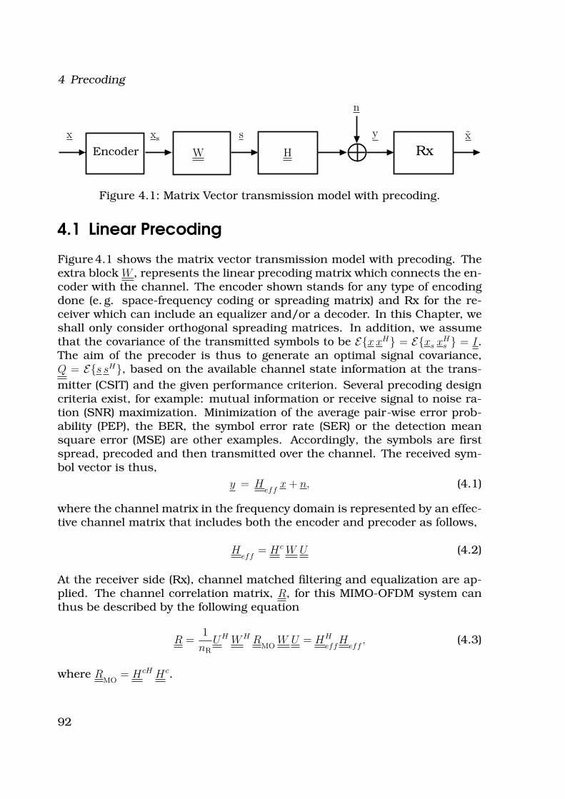
4 Precoding
x xs s
H
n
y x
WEncoder Rx
Figure 4.1: Matrix Vector transmission model with precoding.
4.1 Linear Precoding
Figure 4.1 shows the matrix vector transmission model with precoding. Theextra block W , represents the linear precoding matrix which connects the en-coder with the channel. The encoder shown stands for any type of encodingdone (e. g. space-frequency coding or spreading matrix) and Rx for the re-ceiver which can include an equalizer and/or a decoder. In this Chapter, weshall only consider orthogonal spreading matrices. In addition, we assumethat the covariance of the transmitted symbols to be E{x xH} = E{xs xH
s } = I.The aim of the precoder is thus to generate an optimal signal covariance,Q = E{s sH}, based on the available channel state information at the trans-
mitter (CSIT) and the given performance criterion. Several precoding designcriteria exist, for example: mutual information or receive signal to noise ra-tion (SNR) maximization. Minimization of the average pair-wise error prob-ability (PEP), the BER, the symbol error rate (SER) or the detection meansquare error (MSE) are other examples. Accordingly, the symbols are firstspread, precoded and then transmitted over the channel. The received sym-bol vector is thus,
y = Heff
x + n, (4.1)
where the channel matrix in the frequency domain is represented by an effec-tive channel matrix that includes both the encoder and precoder as follows,
Heff
= Hc W U (4.2)
At the receiver side (Rx), channel matched filtering and equalization are ap-plied. The channel correlation matrix, R, for this MIMO-OFDM system canthus be described by the following equation
R =1
nR
UH WH RMO
W U = HH
effH
eff, (4.3)
where RMO
= HcH Hc.
92
4.2 Full Channel Knowledge at the Transmitter
4.2 Full Channel Knowledge at the Transmitter
In this Section, the channel is assumed to be fully known at both the trans-mitter and the receiver. That is, full CSI is available at both the transmit-ter and the receiver. If the goal is to maximize the mutual information [53],or to minimize the average pairwise error probability (PEP) [76], the sum orweighted sum of the mean square errors (MSE) of all subchannels [77, 78],the precoder is given by,
W = V Λ1/2, (4.4)
where V is obtained by the singular value decomposition (SVD) of the channel
matrix, H = U Σ V H and Λ is the power allocation matrix. At the receiver, alsoassuming full channel knowledge, the signal is left-multiplied by U to obtain
x = Σ s + n, (4.5)
where Σ is a diagonal matrix containing the singular values of the channel
matrix H and s = Λ1/2xs. The covariance matrix of s is Λ and is subjectedto the power constraint: Tr(Λ) = po, where po is available transmit power. Inother words, the channel diagonalizing structure is optimal and V representsthe optimal beam direction for perfect CSIT at the transmitter. The choice ofΛ on the other hand, as we shall show next, depends on the optimizationcriterion. In case of frequency selective channels, the optimum precoderand decoder as shown above can be applied to the individual OFDM sub-channels [78, 79] since this multicarrier approach is known to be capacity-lossless [79].
For other criteria, such as the minimization of the average BER or themaximum MSE, the precoding matrix is given by [77]
W = V Λ1/2UH
Rot, (4.6)
where UH
Rotis a unitary matrix which can be chosen to be any rotation ma-
trix, e. g. Hadamard or DFT matrix [77]. Note that the covariance matrix ofthe transmit signal does not change by UH
Rot. The authors showed that the
MMSE-BLE is the optimal receiver in this case. Again, for frequency selec-tive channels, the results can be directly extended to the individual OFDMsubcarriers [77].
The difference between the above design criteria is whether the objectivefunctions used for optimization are Schur-concave or Schur-convex. ForSchur-convex objective functions, the channel diagonalizing structure(Eqn.4.5) is optimum while for Schur-concave objective functions the diag-onal structure is optimal only in combination with a specific rotation of thetransmitted symbols (Eqn. 4.6) [77].
93
4 Precoding
Power Allocation Strategies
If the goal is to maximize the channel ergodic capacity, then the optimumΛ
optis obtained through the well known water-filling solution on the square
of the channel singular values λi = σ2i [4, 3, 53],
pi =
(
µ − No
λi
)
+
, (4.7)
where No is the noise power, and µ is chosen such that∑
i pi = po and ()+ de-notes max(0, pi). Thus, depending on the amount of available transmit power,some of the weak modes might receive zero power and the signals transmittedin direction of eigenvectors with good eigenvalues are assigned more powerthan those transmitted over eigenvectors corresponding to small eigenvalues.MIMO channel capacity will be discussed in more details in Chapter 5.
Sampath et al. in [78] obtained the optimum linear precoder and decoderusing the weight minimum mean-squared error (weight MMSE) criterion sub-jected to transmit power constraint. As mentioned previously, the optimumlinear precoder and decoder were found to diagonalize the channel into eigensubchannels for any chosen set of error weights. Only the power allocationstrategy is dependent on the error weights. The weight matrix is chosenbased on several design criteria, eg. quality of service (QoS), or equal error(i. e. equal SNR on all subchannels), or information rate maximization (in thiscase, the power allocation is as given in Eqn. 4.7). For example, assumingthe design criterion is the equal error, then the power allocation matrix isgiven by [78],
Λ1/2 =
√
po
Tr(Σ−1)Σ−1/2, (4.8)
If the aim is to minimize the PEP per distance (i. e. minimizing the PEPbased on a given codeword distance, for example the minimum distancecodeword), the optimal solution would be to allocate all of the power to thestrongest eigenmode [76]. In this case, precoding is reduced to single beam-forming and represents an extreme case of selective power allocation. Yet, itmaximizes the receive SNR and extracts the full spatial diversity [22].
4.3 Partial Channel Knowledge at the Transmitter
In this subsection, only partial channel knowledge is assumed at the trans-mitter. In this case, the transmission model in Fig. 4.1 still remains valid.However, the precoding matrix W is not based on the full channel knowl-edge, but only on partial knowledge. We assume that only the transmit
94
4.3 Partial Channel Knowledge at the Transmitter
correlation matrix is known at the transmitter. As aforementioned, this isa well-founded assumption, since, while the channel might be fast changing,the channel correlations remain constant for longer periods of time [74, 75] .
4.3.1 Flat Fading Channels
Several authors have looked at precoding in presence of partial channelknowledge, e. g. [80, 81, 82, 76, 83]. All have found that transmitting inthe direction of the eigenvectors of the transmit correlations is the optimumdirection for both capacity maximization ([80, 82]) and pairwise error proba-bility minimization ([81, 76]). It was shown in [80], that the optimal transmitstrategy for capacity maximization is to transmit along the eigenvectors of thetransmit correlation matrix. The power allocation is done through numericaloptimization and resembles that of waterfilling, where stronger modes areallocated more power than weaker ones. The authors in [82] considered bothtransmit and receive correlations and have shown that, although one stillneeds to transmit in direction of the transmit correlations eigenvectors, theenergy distribution at the transmitter is dependent on both the transmit andreceive correlations. In [84], it was shown that taking the receive correlationsinto account has little to no effect on the BER.
In [81], it was shown that the optimum precoder, w, that minimizes theaverage pairwise error probability for a flat fading MIMO channel employingSTBC encoding is
w = vT
φ vH
C, (4.9)
where kT
= vTeT
vHT
and c cH = vCeC
vHC
and c = x1− x
2is the error matrix
between any two codewords. φ is a diagonal matrix describing the power
allocation strategy for the transmit symbols under the power constraintTr {w wH} = po, where po is the total available power. In this precoding strat-egy, both the error matrix and the transmit correlations are taken into ac-count. For orthogonal STBC, c cH = αI. That is, the code word error matrix isa scaled identity matrix, where α can be chosen to be either the minimum oraverage distance. In this case, v
Ccan be omitted and the precoder reduces
to
w = vT
φ (4.10)
The matrix, φ2, is obtained by waterfilling over the eigenvalues of the channel
correlation matrix [81]. In case of quasi-orthogonal space time block codes(QSTBC), the c cH is not a scaled identity matrix. However, E{c cH} is a scaledidentity matrix and v
Ccan also be omitted if the average distance is consid-
ered [76, 85].
95
4 Precoding
To summarize, we can think of the precoder as a link between the encoderand the channel. The precoder has the task of decorrelating the comingencoded symbols (if the covariance matrix is different from an identity matrix)and adjusting the symbol covariance to that suitable to the channel, basedon the available channel knowledge.
4.3.2 Frequency Selective Channels
Now, we shall extend the above precoding to MIMO-OFDM. As aforemen-tioned, flat fading techniques can be applied to frequency selective channelsby implementing the precoding at the individual subcarriers of the OFDMsystem [21, 76, 77, 86, 87]. We again use the channel matrix in the fre-quency domain from Chapter 3. However, in this Chapter, we shall permutethe channel matrix H such that the entries are grouped by frequency. In thiscase, H is a block diagonal matrix and we denote it by H
B,
Hc
B= K1/2
RH
BK1/2
T, (4.11)
The block matrix HB
is as follows
HB
=
H1
. . . . . . . . . 0...
. . . Hk
. . ....
0 . . . . . . . . . HN
(4.12)
where Hk
are nR × nT matrices containing the channel transfer function atthe kth frequency. The matrices K
Tand K
Rare given by
KT
= IN⊗ k
T(4.13)
KR
= IN⊗ k
R, (4.14)
where ⊗ is the Kronecker product and IN
is the identity matrix of size N ×N .Note that both K
Tand K
Ralways have the same structure as H. That
is, if the elements of H are grouped by frequency, so are KT
and KR
(i. e.K = k ⊗ I
N) as was the case in Chapter 3. Both forms are completely equiv-
alent. However, when spreading is considered, the antenna grouping is amore convenient representation while when precoding is treated grouping byfrequency is the more suitable one.
We make use of the PEP from [88], where the transmit antenna correlationsare included in the Eqn. 3.8.
CY
=L∑
l=0
[
Dl(Cp− E
p)T k∗
T(l)(C
p− E
p)∗D−l
]
⊗ InR
= Y ⊗ InR
, (4.15)
96

4.3 Partial Channel Knowledge at the Transmitter
where Cp
and Ep
are the precoded transmit matrices and kT
is assumed to
be full rank. As mentioned in Chapter 3, Cp
and Ep
are simply obtained by
reshaping the transmit vectors Cp and Ep,
Cp = W C = (IN⊗ w) C =
w C1
w C2...
w CN
=
Cp1
Cp2...
CpN
, (4.16)
where Cj are nT × 1 subvectors of the nTN × 1 transmit vector C. The nT × N
reshaped transmit matrix is thus Cp
=[
Cp1 Cp2 Cpj · · · CpN
]
. We define the
error vector between any two transmit vectors as ∆E = C − E. Thus, afterprecoding and reshaping, the error matrix ∆E
pcan be written as,
∆Ep
= Cp− E
p= w ∆E. (4.17)
Since the eigenvalues CY
are equal to those of Y occurring with nR multiplic-ity (as was also the case in Chapter 3), in all what follows, we concentrateon Y . By precoding at each OFDM subcarrier, assuming that k
T(l) = k
T, the
precoder can be described as follows,
W = IN⊗ w. (4.18)
Our goal is thus to find the precoding matrix W (or equivalently w), to mini-mize the average PEP which is equivalent to maximizing
maxW
J =
rank(Y )∏
i=1
(
1 +Es
4No
λi(Y )
)
, (4.19)
subjected to the power constraint Tr{W WH} = po, and where λi(Y ) are the
eigenvalues of Y . We now proceed as in [81], assuming w = vT
φ vH∆E
, where
∆E ∆EH = v∆E
e∆E
vH∆E
and subsituting Eqn. 4.17 into Y as given in Eqn. 4.15.Accordingly,
Y =L−1∑
l=0
[
Dl∆ET wT k∗
Tw∗∆E∗D−l
]
(4.20)
=L−1∑
l=0
[
Dl∆ET v∗
∆EφT vT
Tk∗
Tv∗
Tφ∗vT
∆E∆E∗D−l
]
=L−1∑
l=0
[
Dl∆ET v∗
∆EφT e
Tφ∗vT
∆E∆E∗D−l
]
= F FH ,
97
4 Precoding
where vTTk∗
Tv∗
T= e
Tand F is given by,
F =[
D0∆ET v∗
∆EφT e1/2
T· · ·DL−1∆ET v∗
∆EφT e1/2
T
]
(4.21)
since the eigenvalues of F FH are equal to those of FHF , we shall now con-sider the latter expression,
FHF =
G GH G D GH · · · GDL−1GH
G D−1GH G GH · · · G DL−2GH
...... G GH ...
G D−(L−1)GH · · · · · · G GH
(4.22)
where
G GH = e1/2
Tφ∗vT
∆E∆E∗∆ET v∗
∆EφT e1/2
T(4.23)
andG DlGH = e1/2
Tφ∗vT
∆E∆E∗Dl ∆ET v∗
∆EφT e1/2
T. (4.24)
As in [76, 85], from now on we shall only look at the average PEP and thusonly consider the average distance (covariance of the error matrix) for theoptimization in Eqn. 4.19. That is, we consider E{∆E ∆EH} = v
∆Ee∆E
vH∆E
,
instead of ∆E ∆EH. Since we assume that all transmit symbols powers are
equal and E{C CH} = I, the E{∆E∗∆ET} = αI, is a scaled identity matrix andthus v
∆Ecan be any arbitrary orthonormal matrix. Accordingly, by taking
the average over all ∆E, we get
G GH = e1/2
Tφ∗vT
∆EE{∆E∗∆ET}v∗
∆EφT e1/2
T= αe1/2
Tφ∗φT e1/2
T, (4.25)
andG DlGH = e1/2
Tφ∗vT
∆EE{∆E∗Dl ∆ET}v∗
∆EφT e1/2
T= 0, (4.26)
since∑
(Dl)ii = 0, and accordingly E{∆E∗Dl ∆ET} = 0. The matrix definedby Eqn. 4.22 thus reduces to a block diagonal matrix. Now, we look again atEqn. 4.19, and using the Hadamard inequality, we can upperbound Eqn. 4.19as follows
J ≤nTL∏
i=1
(
1 +Es
4No
(FHF )ii
)
, (4.27)
where (FHF )ii are the diagonal elements of FHF . The upperbound is achieved
if and only if FHF is diagonal, that is if φ is diagonal. In this case, Eqn.4.27
becomes
J =
nTL∏
i=1
(
1 +αEs
4No
λTiiφ2ii
)
, (4.28)
98
4.4 Uncoded Transmission
where λTii and φii are the diagonal elements of eT
and φ respectively.
Now we look at the power distribution to find the optimum values ofφ2
ii that maximizes J subjected to the power constraint Tr{W WH} = po.Maximizing J is equivalent to maximizing its log, i. e. maximizing
log2(J) =∑nTL
i=1 log2
(
1 + αEs
4NoλTiiφ
2ii
)
and the solution to which is the well
know water-filling method on the eigenvalues of kT
[53, 89]. Thus theoptimum precoder that minimizes the average PEP transmits in the directionof the transmit antenna correlations at each subcarrier and pours power onthe eigenmodes of k
T. As was shown [21], transmitting in the direction of
the transmit antenna correlations at each subcarrier is also the optimumdirection for capacity maximization. In this case however, the optimumpower allocation is obtained through numerical optimization. Nonetheless,it was shown in [21] that waterfilling on the eigenmodes of the transmitcorrelations, although is suboptimal, leads to almost optimal performance.
As aforementioned, v∆E
can be any arbitrary chosen unitary matrix, forexample, as in [81, 76], we can choose v
∆E= I. However, we can consider
our spreading matrices, which are orthonormal, as part of our precoder. Thatis we can write
W = (IN⊗ w) U, (4.29)
as in [77]. As was shown in Sec. 3.6, the spreading matrix, U , as well as thecorrelations affect the amount of interference in the channel. In addition,the BER was shown to also depend on the equalizer employed at the receiver.Similarly, in the case of precoded transmission, the chosen spreading matrix,which although does not affect the covariance of the transmitted symbols, isexpected to affect the BER.
4.4 Uncoded Transmission
In this Section, we look at the BER performance with precoding. As withprevious Chapters, we consider the MMSE-BLE, MMSE-BDFE, RNN, andSCE equalizers. In addition, we also assume a 4 × 4 MIMO channel, withL = 4, N = 32 and uncoded transmission using 4 PSK.
Figures 4.2 and 4.3 show the BER at Eb/No = 14 dB for different spreadingmatrices and the unspread MIMO-OFDM versus the correlation coefficientρ, where the exponential correlation model is assumed, i. e. cij = ρj−i. Thetransmit and receive correlations are assumed equal. For transmission with-out precoding and at low to moderate correlation values, the lowest BER cor-responds to the spreading matrix with highest diversity: MC-CAFS. As the
99
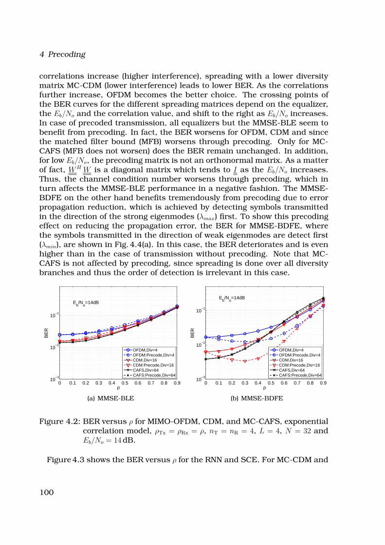
4 Precoding
correlations increase (higher interference), spreading with a lower diversitymatrix MC-CDM (lower interference) leads to lower BER. As the correlationsfurther increase, OFDM becomes the better choice. The crossing points ofthe BER curves for the different spreading matrices depend on the equalizer,the Eb/No and the correlation value, and shift to the right as Eb/No increases.In case of precoded transmission, all equalizers but the MMSE-BLE seem tobenefit from precoding. In fact, the BER worsens for OFDM, CDM and sincethe matched filter bound (MFB) worsens through precoding. Only for MC-CAFS (MFB does not worsen) does the BER remain unchanged. In addition,for low Eb/No, the precoding matrix is not an orthonormal matrix. As a matterof fact, WH W is a diagonal matrix which tends to I as the Eb/No increases.Thus, the channel condition number worsens through precoding, which inturn affects the MMSE-BLE performance in a negative fashion. The MMSE-BDFE on the other hand benefits tremendously from precoding due to errorpropagation reduction, which is achieved by detecting symbols transmittedin the direction of the strong eigenmodes (λmax) first. To show this precodingeffect on reducing the propagation error, the BER for MMSE-BDFE, wherethe symbols transmitted in the direction of weak eigenmodes are detect first(λmin), are shown in Fig. 4.4(a). In this case, the BER deteriorates and is evenhigher than in the case of transmission without precoding. Note that MC-CAFS is not affected by precoding, since spreading is done over all diversitybranches and thus the order of detection is irrelevant in this case.
0 0.1 0.2 0.3 0.4 0.5 0.6 0.7 0.8 0.910
−3
10−2
10−1
ρ
BE
R
Eb/N
o=14dB
OFDM,Div=4OFDM:Precode,Div=4CDM,Div=16CDM:Precode,Div=16CAFS,Div=64CAFS:Precode,Div=64
(a) MMSE-BLE
0 0.1 0.2 0.3 0.4 0.5 0.6 0.7 0.8 0.910
−3
10−2
10−1
ρ
BE
R
Eb/N
o=14dB
OFDM,Div=4OFDM:Precode,Div=4CDM,Div=16CDM:Precode,Div=16CAFS,Div=64CAFS:Precode,Div=64
(b) MMSE-BDFE
Figure 4.2: BER versus ρ for MIMO-OFDM, CDM, and MC-CAFS, exponentialcorrelation model, ρTx = ρRx = ρ, nT = nR = 4, L = 4, N = 32 andEb/No = 14 dB.
Figure 4.3 shows the BER versus ρ for the RNN and SCE. For MC-CDM and
100
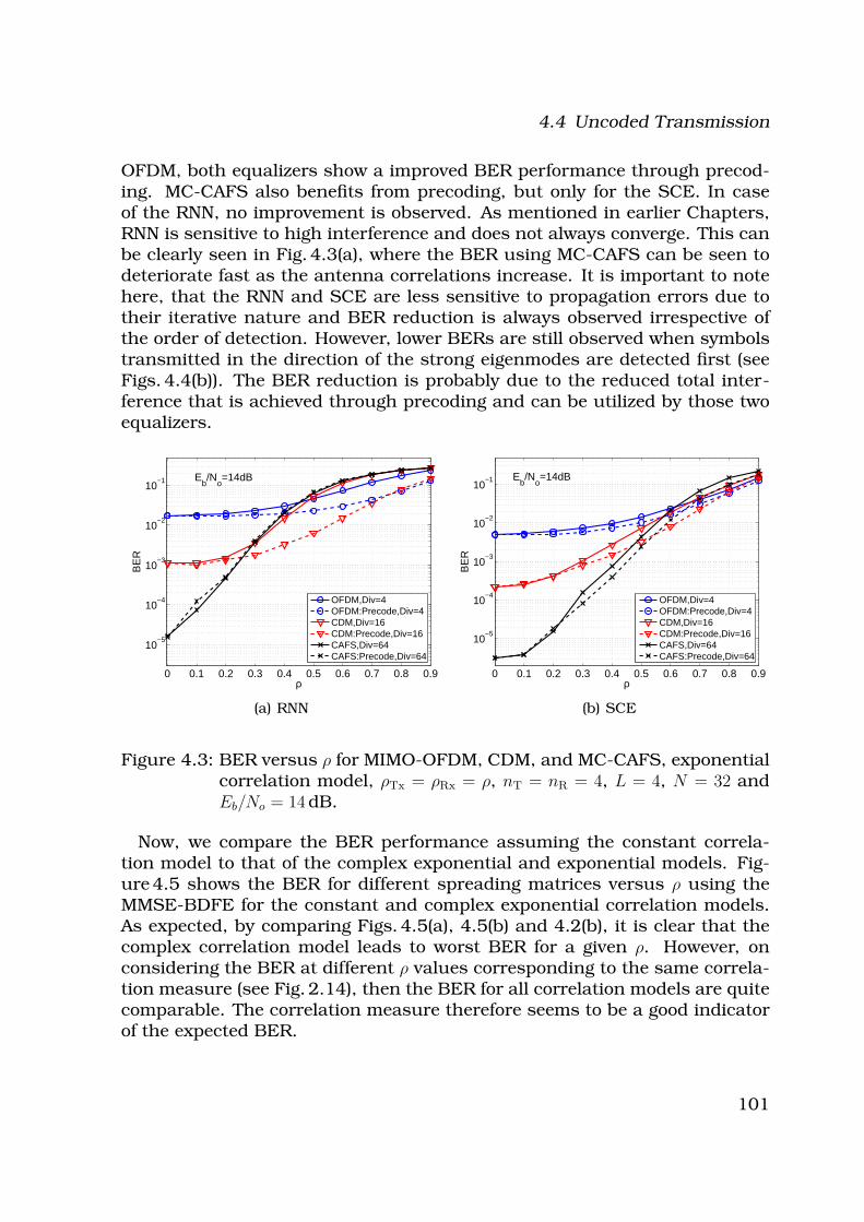
4.4 Uncoded Transmission
OFDM, both equalizers show a improved BER performance through precod-ing. MC-CAFS also benefits from precoding, but only for the SCE. In caseof the RNN, no improvement is observed. As mentioned in earlier Chapters,RNN is sensitive to high interference and does not always converge. This canbe clearly seen in Fig. 4.3(a), where the BER using MC-CAFS can be seen todeteriorate fast as the antenna correlations increase. It is important to notehere, that the RNN and SCE are less sensitive to propagation errors due totheir iterative nature and BER reduction is always observed irrespective ofthe order of detection. However, lower BERs are still observed when symbolstransmitted in the direction of the strong eigenmodes are detected first (seeFigs. 4.4(b)). The BER reduction is probably due to the reduced total inter-ference that is achieved through precoding and can be utilized by those twoequalizers.
0 0.1 0.2 0.3 0.4 0.5 0.6 0.7 0.8 0.9
10−5
10−4
10−3
10−2
10−1
ρ
BE
R
Eb/N
o=14dB
OFDM,Div=4OFDM:Precode,Div=4CDM,Div=16CDM:Precode,Div=16CAFS,Div=64CAFS:Precode,Div=64
(a) RNN
0 0.1 0.2 0.3 0.4 0.5 0.6 0.7 0.8 0.9
10−5
10−4
10−3
10−2
10−1
ρ
BE
RE
b/N
o=14dB
OFDM,Div=4OFDM:Precode,Div=4CDM,Div=16CDM:Precode,Div=16CAFS,Div=64CAFS:Precode,Div=64
(b) SCE
Figure 4.3: BER versus ρ for MIMO-OFDM, CDM, and MC-CAFS, exponentialcorrelation model, ρTx = ρRx = ρ, nT = nR = 4, L = 4, N = 32 andEb/No = 14 dB.
Now, we compare the BER performance assuming the constant correla-tion model to that of the complex exponential and exponential models. Fig-ure 4.5 shows the BER for different spreading matrices versus ρ using theMMSE-BDFE for the constant and complex exponential correlation models.As expected, by comparing Figs. 4.5(a), 4.5(b) and 4.2(b), it is clear that thecomplex correlation model leads to worst BER for a given ρ. However, onconsidering the BER at different ρ values corresponding to the same correla-tion measure (see Fig. 2.14), then the BER for all correlation models are quitecomparable. The correlation measure therefore seems to be a good indicatorof the expected BER.
101
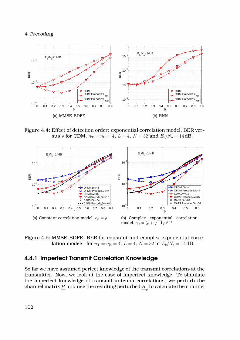
4 Precoding
0 0.1 0.2 0.3 0.4 0.5 0.6 0.7 0.8 0.910
−3
10−2
10−1
ρ
BE
R
Eb/N
o=14dB
CDMCDM:Precode:λ
min
CDM:Precode:λmax
(a) MMSE-BDFE
0 0.1 0.2 0.3 0.4 0.5 0.6 0.7 0.8 0.9
10−4
10−3
10−2
10−1
ρ
BE
R
Eb/N
o=14dB
CDMCDM:Precode:λ
min
CDM:Precode:λmax
(b) RNN
Figure 4.4: Effect of detection order: exponential correlation model, BER ver-sus ρ for CDM, nT = nR = 4, L = 4, N = 32 and Eb/No = 14 dB.
0 0.1 0.2 0.3 0.4 0.5 0.6 0.7 0.8 0.910
−3
10−2
10−1
ρ
BE
R
Eb/N
o=14dB
OFDM,Div=4OFDM:Precode,Div=4CDM,Div=16CDM:Precode,Div=16CAFS,Div=64CAFS:Precode,Div=64
(a) Constant correlation model, cij = ρ
0 0.1 0.2 0.3 0.4 0.5 0.610
−3
10−2
10−1
ρ
BE
R
Eb/N
o=14dB
OFDM,Div=4OFDM:Precode,Div=4CDM,Div=16CDM:Precode,Div=16CAFS,Div=64CAFS:Precode,Div=64
(b) Complex exponential correlationmodel, cij = (ρ +
√−1 ρ)j−i
Figure 4.5: MMSE-BDFE: BER for constant and complex exponential corre-lation models, for nT = nR = 4, L = 4, N = 32 at Eb/No = 14 dB.
4.4.1 Imperfect Transmit Correlation Knowledge
So far we have assumed perfect knowledge of the transmit correlations at thetransmitter. Now, we look at the case of imperfect knowledge. To simulatethe imperfect knowledge of transmit antenna correlations, we perturb thechannel matrix H and use the resulting perturbed H
pto calculate the channel
102
4.4 Uncoded Transmission
correlations [90]. We have opted for this method, since directly perturbing kT
does not guarantee that they remain positive semi-definite. Accordingly, wemodel the perturbed channels as follows,
Hkp
= Hc
k+ E
k(4.30)
where Hkp
and Ek
are the perturbed channel and the perturbation matrix at
the k-th frequency respectively. The elements of Ek
are modeled as uncorre-
lated CN(0,σ2e ). Note that the elements of E
kneed not be uncorrelated. E
kcan
be assumed to have covariance matrix different from a scaled identity ma-trix. By assuming uncorrelated elements, we are investigating the case wherethe transmitter assumes lower correlations than the true ones, especially asσ2
e → 1.0. If we would assume E{EH
kE
k} = σ2
e1nT(an nT × nT matrix of ones)
then we would be looking at the other extreme, where the transmitter as-sumes higher correlations than the true ones. We assume the perturbationsto be independent of the channel coefficients. The channel coefficients arenormalized such that σ2
e + σ2h = 1.0, where σ2
h is the variance of the elementsof Hc
k. Accordingly, the transmit antenna correlations at each frequency are
obtained as follows,
kTe
=1
nR
E{HH
kpH
kp} (4.31)
Based on the above assumptions,
kTe
= σ2hkT
+ σ2eInT
(4.32)
Thus, kTe
= kT
only if σ2e = 0. However, it is not important for k
Tebe exactly
or almost equal to kT, but that the eigenvectors of k
Tediagonalize k
T(i. e.
vTe
≈ vT, where v
Teare the eigenvectors of k
Te). As a measure for that, we
introduce the following norm, Fvv,
Fvv =√
||vHTe
kTv
Te− e
T||2F . (4.33)
If vTe
= vT, then Fvv = 0. The worst case for this model would be to estimate
uncorrelated transmit antennas while the antennas at the transmitter arefully correlated and thus transmitting in direction of eigenmodes with zeroeigenvalues. σ2
e = 1 corresponds to this worst case. For kT
= 1nT
, and kTe
= InT
(vTe
= InT
),
Fvv =√
2nT(nT − 1) = Fmax.
Figure 4.6 show Fvv/Fmax for 100 and 1000 channel realizations used for theestimation of k
T. The exponential correlation model is assumed. The figures
clearly show that for low σ2e values, Fvv remains low. As expected, the higher
103
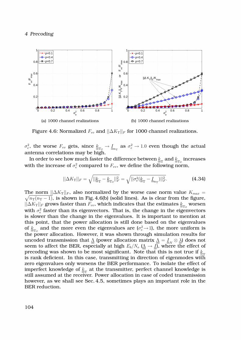
4 Precoding
0 0.2 0.4 0.6 0.8 10
0.2
0.4
0.6
0.8
1
σ2e
Fvv
/Fm
ax
ρ=0.1ρ=0.4ρ=0.7
(a) 1000 channel realizations
0 0.2 0.4 0.6 0.8 10
0.2
0.4
0.6
0.8
1
σ2e
||∆ K
T|| F
/Km
ax
or
F
vv/F
max
||∆ KT||
F/K
max
ρ=0.1ρ=0.4ρ=0.7
(b) 1000 channel realizations
Figure 4.6: Normalized Fvv and ||∆KT||F for 1000 channel realizations.
σ2e , the worse Fvv gets, since k
Te→ I
nTas σ2
e → 1.0 even though the actual
antenna correlations may be high.
In order to see how much faster the difference between kT
and kTe
increases
with the increase of σ2e compared to Fvv, we define the following norm,
||∆KT||F =√
||kT− k
Te||2F =
√
||σ2e(kT
− InT
)||2F . (4.34)
The norm ||∆KT||F , also normalized by the worse case norm value Kmax =√
nT(nT − 1), is shown in Fig. 4.6(b) (solid lines). As is clear from the figure,||∆KT||F grows faster than Fvv, which indicates that the estimates k
Teworsen
with σ2e faster than its eigenvectors. That is, the change in the eigenvectors
is slower than the change in the eigenvalues. It is important to mention atthis point, that the power allocation is still done based on the eigenvaluesof k
Teand the more even the eigenvalues are (σ2
e →1), the more uniform is
the power allocation. However, it was shown through simulation results foruncoded transmission that Λ (power allocation matrix Λ = I
N⊗ λ) does not
seem to affect the BER, especially at high Eb/No (Λ → I), where the effect ofprecoding was shown to be most significant. Note that this is not true if k
Tis rank deficient. In this case, transmitting in direction of eigenmodes withzero eigenvalues only worsens the BER performance. To isolate the effect ofimperfect knowledge of k
Tat the transmitter, perfect channel knowledge is
still assumed at the receiver. Power allocation in case of coded transmissionhowever, as we shall see Sec. 4.5, sometimes plays an important role in theBER reduction.
104
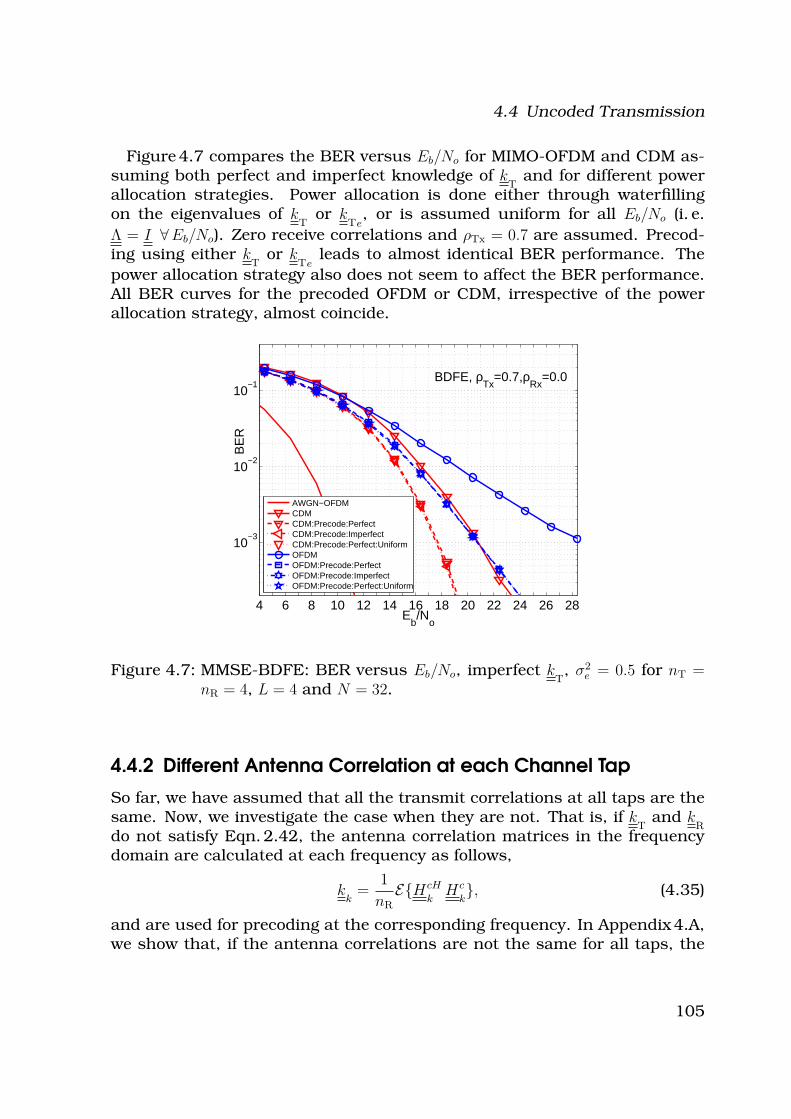
4.4 Uncoded Transmission
Figure 4.7 compares the BER versus Eb/No for MIMO-OFDM and CDM as-suming both perfect and imperfect knowledge of k
Tand for different power
allocation strategies. Power allocation is done either through waterfillingon the eigenvalues of k
Tor k
Te, or is assumed uniform for all Eb/No (i. e.
Λ = I ∀Eb/No). Zero receive correlations and ρTx = 0.7 are assumed. Precod-ing using either k
Tor k
Teleads to almost identical BER performance. The
power allocation strategy also does not seem to affect the BER performance.All BER curves for the precoded OFDM or CDM, irrespective of the powerallocation strategy, almost coincide.
4 6 8 10 12 14 16 18 20 22 24 26 28
10−3
10−2
10−1
Eb/N
o
BE
R
BDFE, ρTx
=0.7,ρRx
=0.0
AWGN−OFDMCDMCDM:Precode:PerfectCDM:Precode:ImperfectCDM:Precode:Perfect:UniformOFDMOFDM:Precode:PerfectOFDM:Precode:ImperfectOFDM:Precode:Perfect:Uniform
Figure 4.7: MMSE-BDFE: BER versus Eb/No, imperfect kT, σ2
e = 0.5 for nT =nR = 4, L = 4 and N = 32.
4.4.2 Different Antenna Correlation at each Channel Tap
So far, we have assumed that all the transmit correlations at all taps are thesame. Now, we investigate the case when they are not. That is, if k
Tand k
Rdo not satisfy Eqn. 2.42, the antenna correlation matrices in the frequencydomain are calculated at each frequency as follows,
kk
=1
nR
E{HcH
kHc
k}, (4.35)
and are used for precoding at the corresponding frequency. In Appendix 4.A,we show that, if the antenna correlations are not the same for all taps, the
105
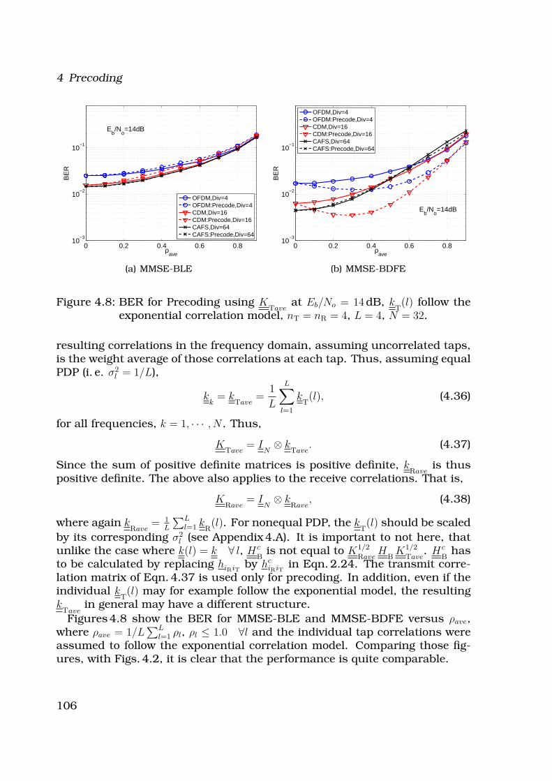
4 Precoding
0 0.2 0.4 0.6 0.810
−3
10−2
10−1
ρave
BE
R
Eb/N
o=14dB
OFDM,Div=4OFDM:Precode,Div=4CDM,Div=16CDM:Precode,Div=16CAFS,Div=64CAFS:Precode,Div=64
(a) MMSE-BLE
0 0.2 0.4 0.6 0.810
−3
10−2
10−1
ρave
BE
R
Eb/N
o=14dB
OFDM,Div=4OFDM:Precode,Div=4CDM,Div=16CDM:Precode,Div=16CAFS,Div=64CAFS:Precode,Div=64
(b) MMSE-BDFE
Figure 4.8: BER for Precoding using KTave
at Eb/No = 14 dB, kT(l) follow the
exponential correlation model, nT = nR = 4, L = 4, N = 32.
resulting correlations in the frequency domain, assuming uncorrelated taps,is the weight average of those correlations at each tap. Thus, assuming equalPDP (i. e. σ2
l = 1/L),
kk
= kTave
=1
L
L∑
l=1
kT(l), (4.36)
for all frequencies, k = 1, · · · , N . Thus,
KTave
= IN⊗ k
Tave. (4.37)
Since the sum of positive definite matrices is positive definite, kRave
is thuspositive definite. The above also applies to the receive correlations. That is,
KRave
= IN⊗ k
Rave, (4.38)
where again kRave
= 1L
∑Ll=1 k
R(l). For nonequal PDP, the k
T(l) should be scaled
by its corresponding σ2l (see Appendix 4.A). It is important to not here, that
unlike the case where k(l) = k ∀ l, Hc
Bis not equal to K1/2
RaveH
BK1/2
Tave. Hc
Bhas
to be calculated by replacing hiRiTby hc
iRiTin Eqn. 2.24. The transmit corre-
lation matrix of Eqn. 4.37 is used only for precoding. In addition, even if theindividual k
T(l) may for example follow the exponential model, the resulting
kTave
in general may have a different structure.
Figures 4.8 show the BER for MMSE-BLE and MMSE-BDFE versus ρave,where ρave = 1/L
∑Ll=1 ρl, ρl ≤ 1.0 ∀l and the individual tap correlations were
assumed to follow the exponential correlation model. Comparing those fig-ures, with Figs. 4.2, it is clear that the performance is quite comparable.
106
4.5 Coded Transmission
4.5 Coded Transmission
In this Section, we first consider coded transmission over time varying chan-nels. We assume a block fading model where the channel remains constantduring the transmission of one codeword. Again, we look at a 4 × 4 MIMOchannel, with L = 4 and transmission using 4 PSK. At the receiver, itera-tive equalization and decoding is performed using either the RNN or SCE asexplained in Chapter 2. We consider the convolutional code with generatorpolynomial [7, 5]8 with memory 2 and rate 1/2. Note that in all what follows,the BER is always plotted versus the transmit Eb/No. That way, the effect oftransmit power distribution can be captured.
Figure 4.9 shows the BER versus the transmit Eb/No using the RNN andSCE equalizers the assuming exponential correlation model. We considerthree cases: ρTx = ρRx = 0.3, ρTx = 0.7, ρRx = 0.0 and ρTx = 0.7, ρRx = 0.7. As ex-pected, the BER deteriorates with increasing correlations. The RNN and SCEhave a very comparable performance for low correlation values (Figs. 4.9(a)and 4.9(b)). Both benefit from precoding only when MC-CAFS spreading isapplied. Precoding with OFDM and MC-CDM leads to worse BERs than with-out.
With increased correlations (ρTx = 0.7), the SCE continues to benefit fromprecoding when MC-CAFS spreading is employed. In case of OFDM and MC-CDM, precoding only improves the performance at low to moderate Eb/No
values. The range of Eb/No values where this improvement is observed in-creases as the amount of correlation present in the channel increases (com-pare Figs. 4.9(b) 4.9(d) and 4.9(f)). However, at high Eb/No, precoding withOFDM and MC-CDM only worsens the BER. The RNN on the other hand, ex-hibits a totally different behavior. Precoding with MC-CDM spreading seemsnow to improve the BER. When correlations are high at both the transmitterand receiver (ρTx = ρRx = 0.7), precoding with OFDM also leads to improvedBER performance.
To better understand the behavior of those equalizers as part of the itera-tive equalization and decoding loop, we shall now consider the EXIT chartsas an analysis tool. However, in order for the EXIT charts to make sense,we have to consider one channel at a time, and look at the EXIT chart foreach channel realization. Due to the computational complexity and volumeinvolved, we instead look at three MIMO 4 × 4 channel groups:
- Group 1 with four channels having low correlations at both the transmitterand receiver ρTx = ρRx = 0.3.- Group 2 with four channels having high correlations at the transmitter andzero receive correlations ρTx = 0.7, ρRx = 0.0.
- Group 3 also with four channels having high correlations at both the trans-
107
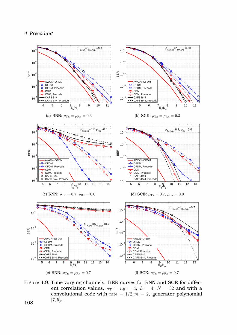
4 Precoding
4 5 6 7 8 9 10 11
10−5
10−4
10−3
10−2
10−1
Eb/N
o
BE
R
ρTx,exp
=ρRx,exp
=0.3
AWGN−OFDMOFDMOFDM, PrecodeCDMCDM, PrecodeCAFS B=4CAFS B=4, Precode
(a) RNN: ρTx = ρRx = 0.3
4 5 6 7 8 9 10 11
10−5
10−4
10−3
10−2
10−1
Eb/N
o
BE
R
ρTx,exp
=ρRx,exp
=0.3
AWGN−OFDMOFDMOFDM, PrecodeCDMCDM, PrecodeCAFS B=4CAFS B=4, Precode
(b) SCE: ρTx = ρRx = 0.3
5 6 7 8 9 10 11 12 13 1410
−5
10−4
10−3
10−2
10−1
Eb/N
o
BE
R
ρTx,exp
=0.7, ρRx
=0.0
AWGN−OFDMOFDMOFDM, PrecodeCDMCDM, PrecodeCAFS B=4CAFS B=4, Precode
(c) RNN: ρTx = 0.7, ρRx = 0.0
5 6 7 8 9 10 11 12 1310
−5
10−4
10−3
10−2
10−1
Eb/N
o
BE
R
ρTx,exp
=0.7, ρRx
=0.0
AWGN−OFDMOFDMOFDM, PrecodeCDMCDM, PrecodeCAFS B=4CAFS B=4, Precode
(d) SCE: ρTx = 0.7, ρRx = 0.0
5 6 7 8 9 10 11 12 13 1410
−4
10−3
10−2
10−1
Eb/N
o
BE
R
ρTx,exp
=ρRx,exp
=0.7
AWGN−OFDMOFDMOFDM, PrecodeCDMCDM, PrecodeCAFS B=4CAFS B=4, Precode
(e) RNN: ρTx = ρRx = 0.7
5 6 7 8 9 10 11 12 13
10−5
10−4
10−3
10−2
10−1
Eb/N
o
BE
R
ρTx,exp
=ρRx,exp
=0.7
AWGN−OFDMOFDMOFDM, PrecodeCDMCDM, PrecodeCAFS B=4CAFS B=4, Precode
(f) SCE: ρTx = ρRx = 0.7
Figure 4.9: Time varying channels: BER curves for RNN and SCE for differ-ent correlation values, nT = nR = 4, L = 4, N = 32 and with aconvolutional code with rate = 1/2,m = 2, generator polynomial[7, 5]8.108
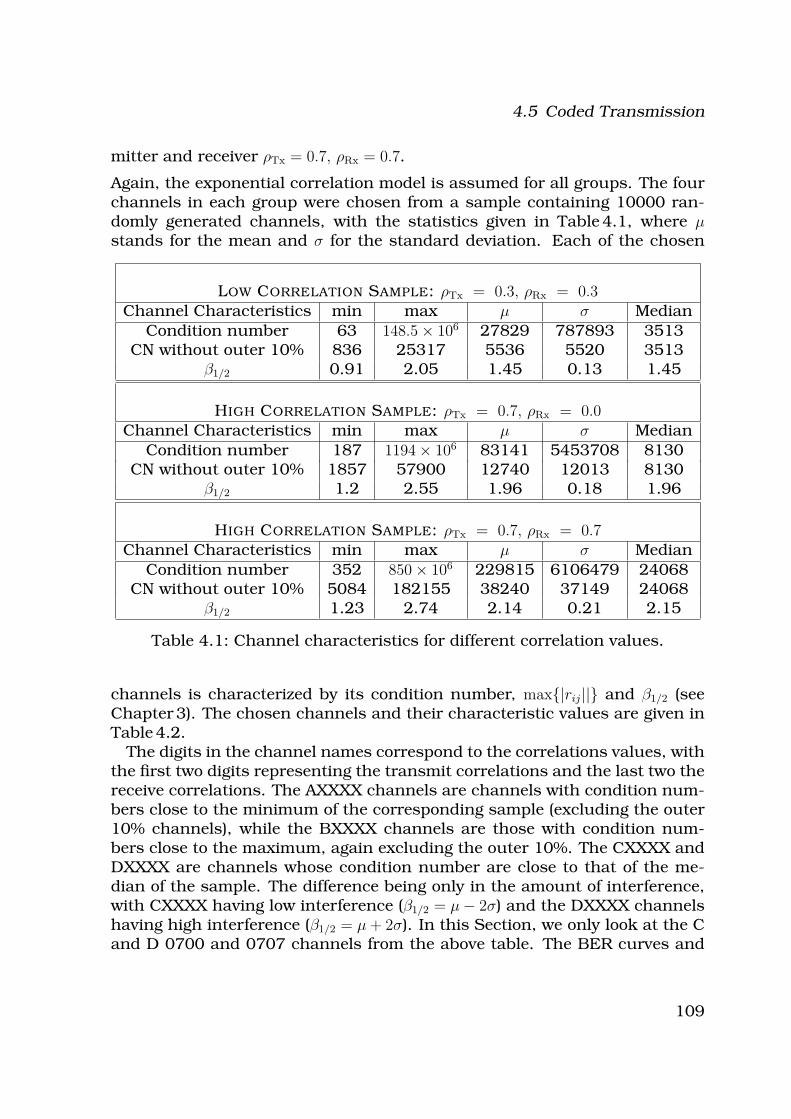
4.5 Coded Transmission
mitter and receiver ρTx = 0.7, ρRx = 0.7.
Again, the exponential correlation model is assumed for all groups. The fourchannels in each group were chosen from a sample containing 10000 ran-domly generated channels, with the statistics given in Table 4.1, where µstands for the mean and σ for the standard deviation. Each of the chosen
LOW CORRELATION SAMPLE: ρTx = 0.3, ρRx = 0.3Channel Characteristics min max µ σ Median
Condition number 63 148.5 × 10⁶ 27829 787893 3513CN without outer 10% 836 25317 5536 5520 3513
β1/2 0.91 2.05 1.45 0.13 1.45
HIGH CORRELATION SAMPLE: ρTx = 0.7, ρRx = 0.0Channel Characteristics min max µ σ Median
Condition number 187 1194 × 106 83141 5453708 8130CN without outer 10% 1857 57900 12740 12013 8130
β1/2 1.2 2.55 1.96 0.18 1.96
HIGH CORRELATION SAMPLE: ρTx = 0.7, ρRx = 0.7Channel Characteristics min max µ σ Median
Condition number 352 850 × 106 229815 6106479 24068CN without outer 10% 5084 182155 38240 37149 24068
β1/2 1.23 2.74 2.14 0.21 2.15
Table 4.1: Channel characteristics for different correlation values.
channels is characterized by its condition number, max{|rij||} and β1/2 (seeChapter 3). The chosen channels and their characteristic values are given inTable 4.2.
The digits in the channel names correspond to the correlations values, withthe first two digits representing the transmit correlations and the last two thereceive correlations. The AXXXX channels are channels with condition num-bers close to the minimum of the corresponding sample (excluding the outer10% channels), while the BXXXX channels are those with condition num-bers close to the maximum, again excluding the outer 10%. The CXXXX andDXXXX are channels whose condition number are close to that of the me-dian of the sample. The difference being only in the amount of interference,with CXXXX having low interference (β1/2 = µ − 2σ) and the DXXXX channelshaving high interference (β1/2 = µ + 2σ). In this Section, we only look at the Cand D 0700 and 0707 channels from the above table. The BER curves and
109
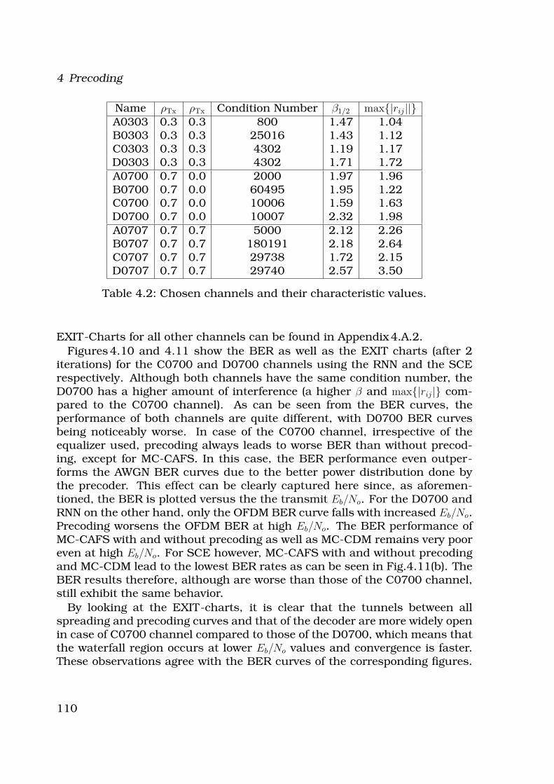
4 Precoding
Name ρTx ρTx Condition Number β1/2 max{|rij||}A0303 0.3 0.3 800 1.47 1.04B0303 0.3 0.3 25016 1.43 1.12C0303 0.3 0.3 4302 1.19 1.17D0303 0.3 0.3 4302 1.71 1.72
A0700 0.7 0.0 2000 1.97 1.96B0700 0.7 0.0 60495 1.95 1.22C0700 0.7 0.0 10006 1.59 1.63D0700 0.7 0.0 10007 2.32 1.98
A0707 0.7 0.7 5000 2.12 2.26B0707 0.7 0.7 180191 2.18 2.64C0707 0.7 0.7 29738 1.72 2.15D0707 0.7 0.7 29740 2.57 3.50
Table 4.2: Chosen channels and their characteristic values.
EXIT-Charts for all other channels can be found in Appendix 4.A.2.
Figures 4.10 and 4.11 show the BER as well as the EXIT charts (after 2iterations) for the C0700 and D0700 channels using the RNN and the SCErespectively. Although both channels have the same condition number, theD0700 has a higher amount of interference (a higher β and max{|rij|} com-pared to the C0700 channel). As can be seen from the BER curves, theperformance of both channels are quite different, with D0700 BER curvesbeing noticeably worse. In case of the C0700 channel, irrespective of theequalizer used, precoding always leads to worse BER than without precod-ing, except for MC-CAFS. In this case, the BER performance even outper-forms the AWGN BER curves due to the better power distribution done bythe precoder. This effect can be clearly captured here since, as aforemen-tioned, the BER is plotted versus the the transmit Eb/No. For the D0700 andRNN on the other hand, only the OFDM BER curve falls with increased Eb/No.Precoding worsens the OFDM BER at high Eb/No. The BER performance ofMC-CAFS with and without precoding as well as MC-CDM remains very pooreven at high Eb/No. For SCE however, MC-CAFS with and without precodingand MC-CDM lead to the lowest BER rates as can be seen in Fig.4.11(b). TheBER results therefore, although are worse than those of the C0700 channel,still exhibit the same behavior.
By looking at the EXIT-charts, it is clear that the tunnels between allspreading and precoding curves and that of the decoder are more widely openin case of C0700 channel compared to those of the D0700, which means thatthe waterfall region occurs at lower Eb/No values and convergence is faster.These observations agree with the BER curves of the corresponding figures.
110
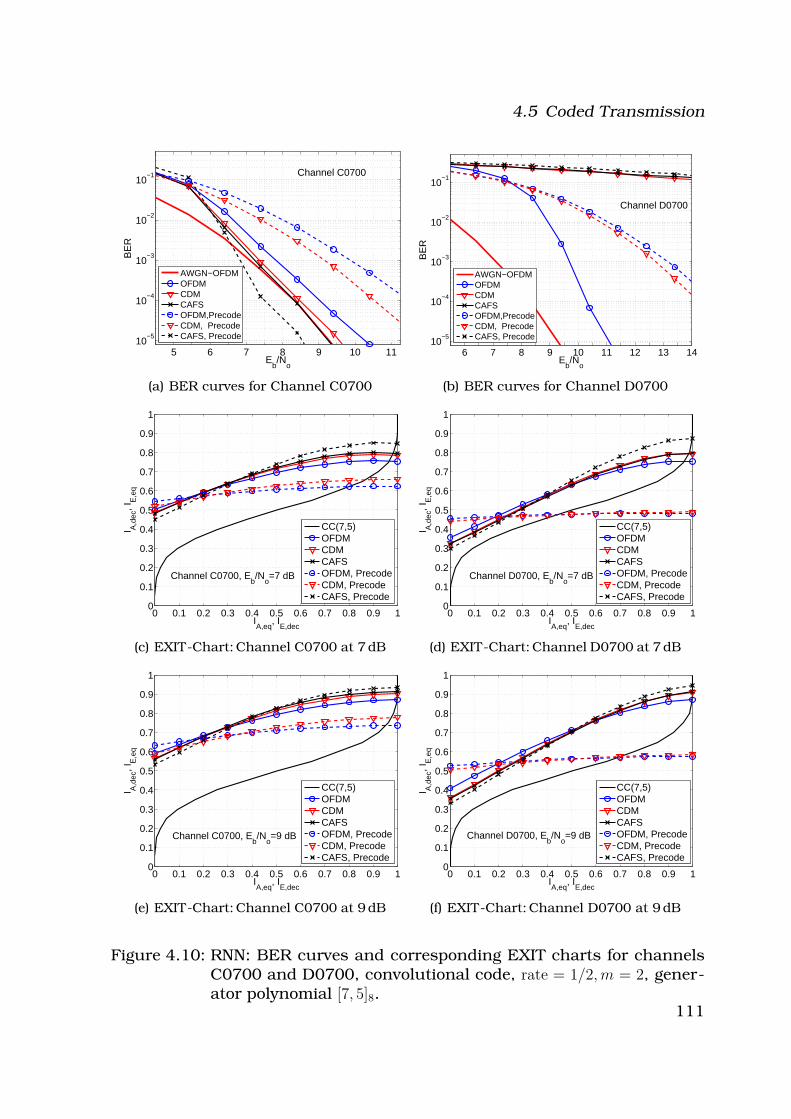
4.5 Coded Transmission
5 6 7 8 9 10 1110
−5
10−4
10−3
10−2
10−1
Eb/N
o
BE
R
Channel C0700
AWGN−OFDMOFDMCDMCAFSOFDM,PrecodeCDM, PrecodeCAFS, Precode
(a) BER curves for Channel C0700
6 7 8 9 10 11 12 13 1410
−5
10−4
10−3
10−2
10−1
Eb/N
o
BE
R
Channel D0700
AWGN−OFDMOFDMCDMCAFSOFDM,PrecodeCDM, PrecodeCAFS, Precode
(b) BER curves for Channel D0700
0 0.1 0.2 0.3 0.4 0.5 0.6 0.7 0.8 0.9 10
0.1
0.2
0.3
0.4
0.5
0.6
0.7
0.8
0.9
1
IA,eq
, IE,dec
I A,d
ec, I
E,e
q
Channel C0700, Eb/N
o=7 dB
CC(7,5)OFDMCDMCAFSOFDM, PrecodeCDM, PrecodeCAFS, Precode
(c) EXIT-Chart: Channel C0700 at 7 dB
0 0.1 0.2 0.3 0.4 0.5 0.6 0.7 0.8 0.9 10
0.1
0.2
0.3
0.4
0.5
0.6
0.7
0.8
0.9
1
IA,eq
, IE,dec
I A,d
ec, I
E,e
q
Channel D0700, Eb/N
o=7 dB
CC(7,5)OFDMCDMCAFSOFDM, PrecodeCDM, PrecodeCAFS, Precode
(d) EXIT-Chart: Channel D0700 at 7 dB
0 0.1 0.2 0.3 0.4 0.5 0.6 0.7 0.8 0.9 10
0.1
0.2
0.3
0.4
0.5
0.6
0.7
0.8
0.9
1
IA,eq
, IE,dec
I A,d
ec, I
E,e
q
Channel C0700, Eb/N
o=9 dB
CC(7,5)OFDMCDMCAFSOFDM, PrecodeCDM, PrecodeCAFS, Precode
(e) EXIT-Chart: Channel C0700 at 9 dB
0 0.1 0.2 0.3 0.4 0.5 0.6 0.7 0.8 0.9 10
0.1
0.2
0.3
0.4
0.5
0.6
0.7
0.8
0.9
1
IA,eq
, IE,dec
I A,d
ec, I
E,e
q
Channel D0700, Eb/N
o=9 dB
CC(7,5)OFDMCDMCAFSOFDM, PrecodeCDM, PrecodeCAFS, Precode
(f) EXIT-Chart: Channel D0700 at 9 dB
Figure 4.10: RNN: BER curves and corresponding EXIT charts for channelsC0700 and D0700, convolutional code, rate = 1/2,m = 2, gener-ator polynomial [7, 5]8.
111
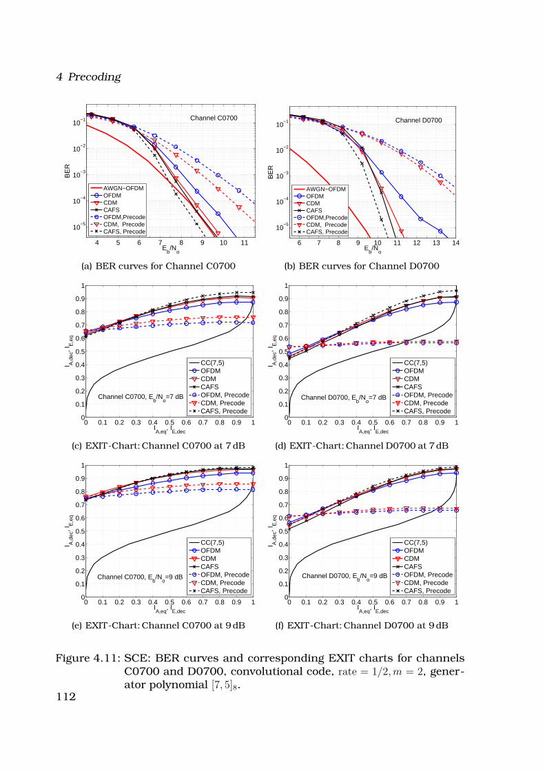
4 Precoding
4 5 6 7 8 9 10 11
10−5
10−4
10−3
10−2
10−1
Eb/N
o
BE
R
Channel C0700
AWGN−OFDMOFDMCDMCAFSOFDM,PrecodeCDM, PrecodeCAFS, Precode
(a) BER curves for Channel C0700
6 7 8 9 10 11 12 13 14
10−5
10−4
10−3
10−2
10−1
Eb/N
o
BE
R
Channel D0700
AWGN−OFDMOFDMCDMCAFSOFDM,PrecodeCDM, PrecodeCAFS, Precode
(b) BER curves for Channel D0700
0 0.1 0.2 0.3 0.4 0.5 0.6 0.7 0.8 0.9 10
0.1
0.2
0.3
0.4
0.5
0.6
0.7
0.8
0.9
1
IA,eq
, IE,dec
I A,d
ec, I
E,e
q
Channel C0700, Eb/N
o=7 dB
CC(7,5)OFDMCDMCAFSOFDM, PrecodeCDM, PrecodeCAFS, Precode
(c) EXIT-Chart: Channel C0700 at 7 dB
0 0.1 0.2 0.3 0.4 0.5 0.6 0.7 0.8 0.9 10
0.1
0.2
0.3
0.4
0.5
0.6
0.7
0.8
0.9
1
IA,eq
, IE,dec
I A,d
ec, I
E,e
q
Channel D0700, Eb/N
o=7 dB
CC(7,5)OFDMCDMCAFSOFDM, PrecodeCDM, PrecodeCAFS, Precode
(d) EXIT-Chart: Channel D0700 at 7 dB
0 0.1 0.2 0.3 0.4 0.5 0.6 0.7 0.8 0.9 10
0.1
0.2
0.3
0.4
0.5
0.6
0.7
0.8
0.9
1
IA,eq
, IE,dec
I A,d
ec, I
E,e
q
Channel C0700, Eb/N
o=9 dB
CC(7,5)OFDMCDMCAFSOFDM, PrecodeCDM, PrecodeCAFS, Precode
(e) EXIT-Chart: Channel C0700 at 9 dB
0 0.1 0.2 0.3 0.4 0.5 0.6 0.7 0.8 0.9 10
0.1
0.2
0.3
0.4
0.5
0.6
0.7
0.8
0.9
1
IA,eq
, IE,dec
I A,d
ec, I
E,e
q
Channel D0700, Eb/N
o=9 dB
CC(7,5)OFDMCDMCAFSOFDM, PrecodeCDM, PrecodeCAFS, Precode
(f) EXIT-Chart: Channel D0700 at 9 dB
Figure 4.11: SCE: BER curves and corresponding EXIT charts for channelsC0700 and D0700, convolutional code, rate = 1/2,m = 2, gener-ator polynomial [7, 5]8.
112
4.5 Coded Transmission
We can also see that the starting point (IA,dec at IE,dec = 0) for OFDM and CDMfor the precoded case are higher than those without precoding. As mentionedin Chapter 2, this initial point is dependent on the amount of interference inthe channel, being higher for less interference. This is especially importantwhen the tunnel opening is small i. e. at low Eb/No. Since precoding reducesthe amount of total interference, the starting point shifts upwards, whichexplains why precoding with OFDM and MC-CDM improves the BER at lowEb/No. On the other hand, the intersection points between those curves andthat of the decoder become more important as Eb/No increases (wider tun-nel). This intersection point is dependent on the MFB, and shifts to the rightas the MFB improves. Since the hard decisions are made after the decoder,a higher IE,dec at the intersection point means in general better BER. Thisexplains why the OFDM and MC-CDM do not converge to the AWGN perfor-mance as the Eb/No increases. The starting points for all EXIT-chart curvesin case of SCE are higher than for those of the RNN at the same Eb/No. Inaddition, the SCE EXIT-charts tunnel openings are wider than those of theRNN. Both factors thus explain the better BER performance and the fasterconvergence using the SCE.
Figures 4.12 and 4.13 show the BER curves and corresponding EXIT-charts for the C0707 and D0707 channels again using the RNN and SCErespectively. Due to the presence of the receive correlations, the amountof interference increases compared to the C0700 and D0700 channels (seeChapter 3). Due to increased interference values, both the RNN and SCE BERcurves converge slower and the waterfall region starts at later Eb/No valuescompared to the 0700 channels. For the D0707, the BER remain very higheven at Eb/No = 11 dB for both equalizers. In case of the RNN, and as can beseen in the EXIT-charts in Figs. 4.12(d) and 4.12(f), that even at 13 dB, thecurves of the MC-CDM, MC-CAFS with and without precoding lie below thatof the decoder. That is, the tunnel is closed and no exchange of informationis possible between the RNN and the decoder. As a result, the BER remainsvery high (almost 0.4). A tunnel opening exists for OFDM with and withoutprecoding and MC-CDM with precoding. As can be seen in Fig. 4.12(f), al-though the intersection point of OFDM without precoding with the decodercurve occurs at higher IE,dec value than for OFDM with precoding, the BER isworse. This can be explain by looking at the IA,dec value at IE,dec = 0, whichis lower in case of OFDM without precoding than for OFDM with precoding.The starting point seems to be a more important factor even at this Eb/No
due to the high amount of interference. All of the above can be applied to theSCE, except that the tunnels are already open at much lower Eb/No valuescompared to the RNN equalizer.
In case of the C0707 channel, the tunnels for all spreading and precod-ing curves are open and convergence can be seen to occur at much lower
113
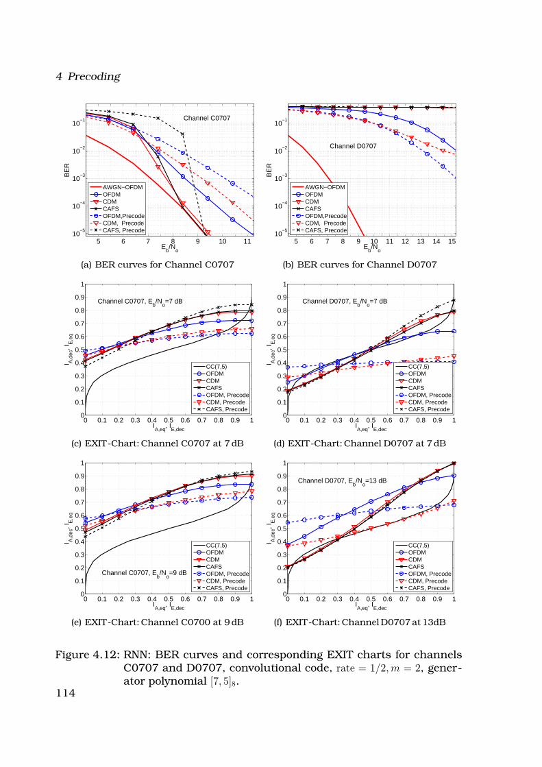
4 Precoding
5 6 7 8 9 10 1110
−5
10−4
10−3
10−2
10−1
Eb/N
o
BE
R
Channel C0707
AWGN−OFDMOFDMCDMCAFSOFDM,PrecodeCDM, PrecodeCAFS, Precode
(a) BER curves for Channel C0707
5 6 7 8 9 10 11 12 13 14 1510
−5
10−4
10−3
10−2
10−1
Eb/N
o
BE
R
Channel D0707
AWGN−OFDMOFDMCDMCAFSOFDM,PrecodeCDM, PrecodeCAFS, Precode
(b) BER curves for Channel D0707
0 0.1 0.2 0.3 0.4 0.5 0.6 0.7 0.8 0.9 10
0.1
0.2
0.3
0.4
0.5
0.6
0.7
0.8
0.9
1
IA,eq
, IE,dec
I A,d
ec, I
E,e
q
Channel C0707, Eb/N
o=7 dB
CC(7,5)OFDMCDMCAFSOFDM, PrecodeCDM, PrecodeCAFS, Precode
(c) EXIT-Chart: Channel C0707 at 7 dB
0 0.1 0.2 0.3 0.4 0.5 0.6 0.7 0.8 0.9 10
0.1
0.2
0.3
0.4
0.5
0.6
0.7
0.8
0.9
1
IA,eq
, IE,dec
I A,d
ec, I
E,e
q
Channel D0707, Eb/N
o=7 dB
CC(7,5)OFDMCDMCAFSOFDM, PrecodeCDM, PrecodeCAFS, Precode
(d) EXIT-Chart: Channel D0707 at 7 dB
0 0.1 0.2 0.3 0.4 0.5 0.6 0.7 0.8 0.9 10
0.1
0.2
0.3
0.4
0.5
0.6
0.7
0.8
0.9
1
IA,eq
, IE,dec
I A,d
ec, I
E,e
q
Channel C0707, Eb/N
o=9 dB
CC(7,5)OFDMCDMCAFSOFDM, PrecodeCDM, PrecodeCAFS, Precode
(e) EXIT-Chart: Channel C0700 at 9 dB
0 0.1 0.2 0.3 0.4 0.5 0.6 0.7 0.8 0.9 10
0.1
0.2
0.3
0.4
0.5
0.6
0.7
0.8
0.9
1
IA,eq
, IE,dec
I A,d
ec, I
E,e
q
Channel D0707, Eb/N
o=13 dB
CC(7,5)OFDMCDMCAFSOFDM, PrecodeCDM, PrecodeCAFS, Precode
(f) EXIT-Chart: Channel D0707 at 13dB
Figure 4.12: RNN: BER curves and corresponding EXIT charts for channelsC0707 and D0707, convolutional code, rate = 1/2,m = 2, gener-ator polynomial [7, 5]8.
114
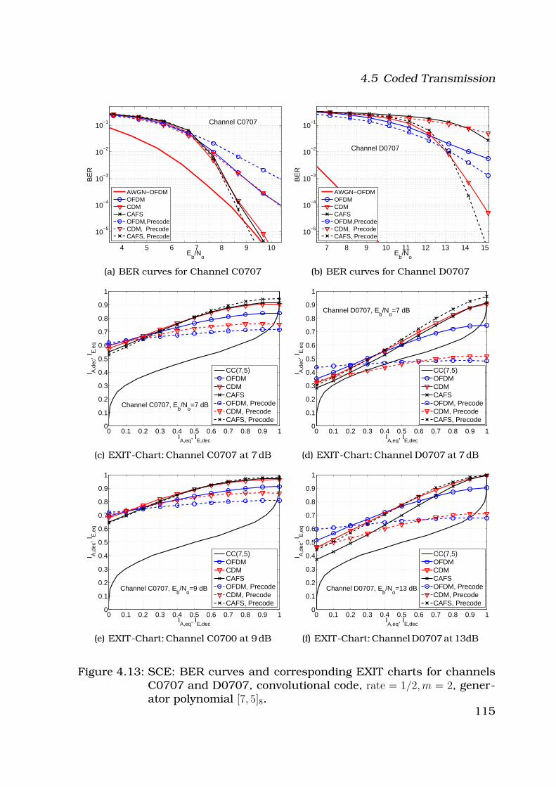
4.5 Coded Transmission
4 5 6 7 8 9 10
10−5
10−4
10−3
10−2
10−1
Eb/N
o
BE
R
Channel C0707
AWGN−OFDMOFDMCDMCAFSOFDM,PrecodeCDM, PrecodeCAFS, Precode
(a) BER curves for Channel C0707
7 8 9 10 11 12 13 14 15
10−5
10−4
10−3
10−2
10−1
Eb/N
o
BE
R
Channel D0707
AWGN−OFDMOFDMCDMCAFSOFDM,PrecodeCDM, PrecodeCAFS, Precode
(b) BER curves for Channel D0707
0 0.1 0.2 0.3 0.4 0.5 0.6 0.7 0.8 0.9 10
0.1
0.2
0.3
0.4
0.5
0.6
0.7
0.8
0.9
1
IA,eq
, IE,dec
I A,d
ec, I
E,e
q
Channel C0707, Eb/N
o=7 dB
CC(7,5)OFDMCDMCAFSOFDM, PrecodeCDM, PrecodeCAFS, Precode
(c) EXIT-Chart: Channel C0707 at 7 dB
0 0.1 0.2 0.3 0.4 0.5 0.6 0.7 0.8 0.9 10
0.1
0.2
0.3
0.4
0.5
0.6
0.7
0.8
0.9
1
IA,eq
, IE,dec
I A,d
ec, I
E,e
q
Channel D0707, Eb/N
o=7 dB
CC(7,5)OFDMCDMCAFSOFDM, PrecodeCDM, PrecodeCAFS, Precode
(d) EXIT-Chart: Channel D0707 at 7 dB
0 0.1 0.2 0.3 0.4 0.5 0.6 0.7 0.8 0.9 10
0.1
0.2
0.3
0.4
0.5
0.6
0.7
0.8
0.9
1
IA,eq
, IE,dec
I A,d
ec, I
E,e
q
Channel C0707, Eb/N
o=9 dB
CC(7,5)OFDMCDMCAFSOFDM, PrecodeCDM, PrecodeCAFS, Precode
(e) EXIT-Chart: Channel C0700 at 9 dB
0 0.1 0.2 0.3 0.4 0.5 0.6 0.7 0.8 0.9 10
0.1
0.2
0.3
0.4
0.5
0.6
0.7
0.8
0.9
1
IA,eq
, IE,dec
I A,d
ec, I
E,e
q
Channel D0707, Eb/N
o=13 dB
CC(7,5)OFDMCDMCAFSOFDM, PrecodeCDM, PrecodeCAFS, Precode
(f) EXIT-Chart: Channel D0707 at 13dB
Figure 4.13: SCE: BER curves and corresponding EXIT charts for channelsC0707 and D0707, convolutional code, rate = 1/2,m = 2, gener-ator polynomial [7, 5]8.
115
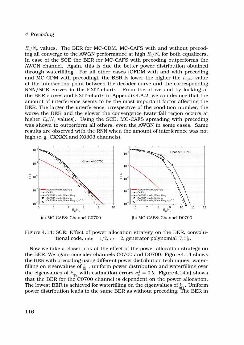
4 Precoding
Eb/No values. The BER for MC-CDM, MC-CAFS with and without precod-ing all converge to the AWGN performance at high Eb/No for both equalizers.In case of the SCE the BER for MC-CAFS with precoding outperforms theAWGN channel. Again, this is due the better power distribution obtainedthrough waterfilling. For all other cases (OFDM with and with precodingand MC-CDM with precoding), the BER is lower the higher the IE,dec valueat the intersection point between the decoder curve and the correspondingRNN/SCE curves in the EXIT-charts. From the above and by looking atthe BER curves and EXIT-charts in Appendix 4.A.2, we can deduce that theamount of interference seems to be the most important factor affecting theBER. The larger the interference, irrespective of the condition number, theworse the BER and the slower the convergence (waterfall region occurs athigher Eb/No values). Using the SCE, MC-CAFS spreading with precodingwas shown to outperform all others, even the AWGN in some cases. Sameresults are observed with the RNN when the amount of interference was nothigh (e. g. CXXXX and X0303 channels).
5 6 7 8 9 1010
−5
10−4
10−3
10−2
10−1
Eb/N
o
BE
R
Channel C0700
AWGN−OFDM, rate=1/2CAFSCAFS:Precode, WaterfillingCAFS:Precode, UniformCAFS:Precode, Waterfilling, σ2
e=0.5
(a) MC-CAFS: Channel C0700
6 7 8 9 10 11 1210
−5
10−4
10−3
10−2
10−1
Eb/N
o
BE
R
Channel D0700
AWGN−OFDM, rate=1/2CAFSCAFS:Precode, WaterfillingCAFS:Precode, UniformCAFS:Precode, Waterfilling, σ2
e=0.5
(b) MC-CAFS: Channel D0700
Figure 4.14: SCE: Effect of power allocation strategy on the BER, convolu-tional code, rate = 1/2, m = 2, generator polynomial [7, 5]8.
Now we take a closer look at the effect of the power allocation strategy onthe BER. We again consider channels C0700 and D0700. Figure 4.14 showsthe BER with precoding using different power distribution techniques: water-filling on eigenvalues of k
T, uniform power distribution and waterfilling over
the eigenvalues of kTe
with estimation errors σ2e = 0.5. Figure 4.14(a) shows
that the BER for the C0700 channel is dependent on the power allocation.The lowest BER is achieved for waterfilling on the eigenvalues of k
T. Uniform
power distribution leads to the same BER as without precoding. The BER in
116
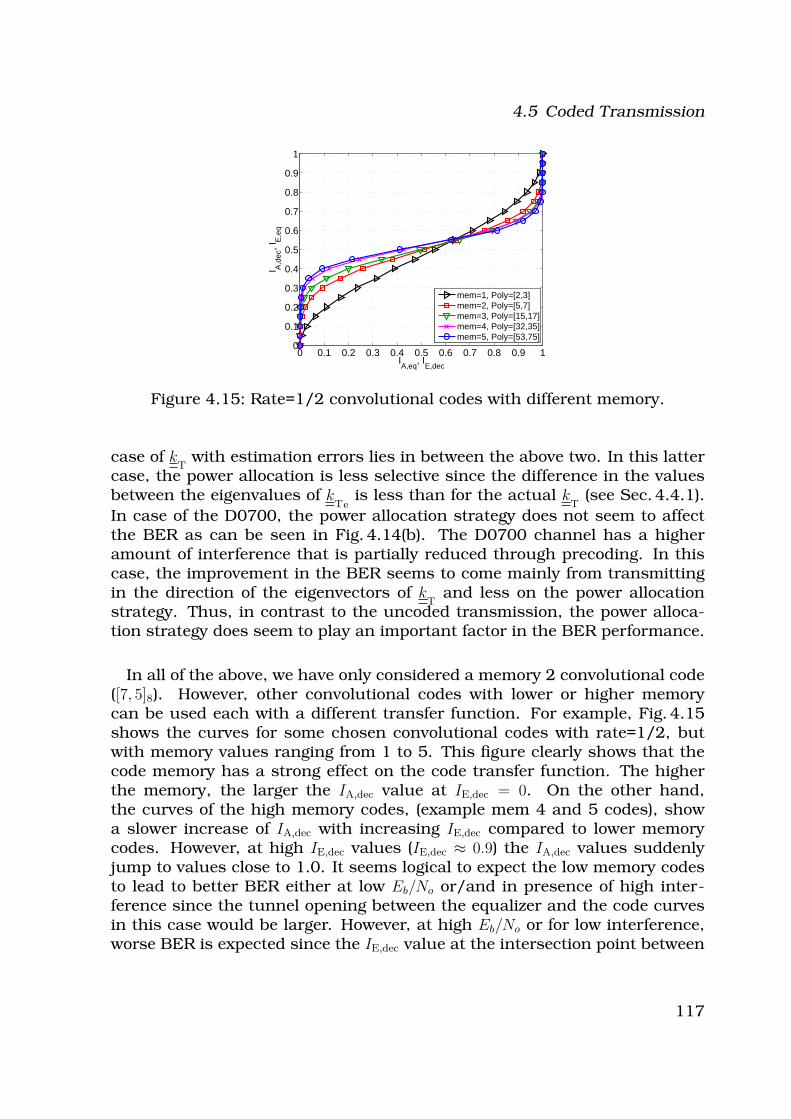
4.5 Coded Transmission
0 0.1 0.2 0.3 0.4 0.5 0.6 0.7 0.8 0.9 10
0.1
0.2
0.3
0.4
0.5
0.6
0.7
0.8
0.9
1
IA,eq
, IE,dec
I A,d
ec, I
E,e
q
mem=1, Poly=[2,3]mem=2, Poly=[5,7]mem=3, Poly=[15,17]mem=4, Poly=[32,35]mem=5, Poly=[53,75]
Figure 4.15: Rate=1/2 convolutional codes with different memory.
case of kT
with estimation errors lies in between the above two. In this lattercase, the power allocation is less selective since the difference in the valuesbetween the eigenvalues of k
Teis less than for the actual k
T(see Sec. 4.4.1).
In case of the D0700, the power allocation strategy does not seem to affectthe BER as can be seen in Fig. 4.14(b). The D0700 channel has a higheramount of interference that is partially reduced through precoding. In thiscase, the improvement in the BER seems to come mainly from transmittingin the direction of the eigenvectors of k
Tand less on the power allocation
strategy. Thus, in contrast to the uncoded transmission, the power alloca-tion strategy does seem to play an important factor in the BER performance.
In all of the above, we have only considered a memory 2 convolutional code([7, 5]8). However, other convolutional codes with lower or higher memorycan be used each with a different transfer function. For example, Fig. 4.15shows the curves for some chosen convolutional codes with rate=1/2, butwith memory values ranging from 1 to 5. This figure clearly shows that thecode memory has a strong effect on the code transfer function. The higherthe memory, the larger the IA,dec value at IE,dec = 0. On the other hand,the curves of the high memory codes, (example mem 4 and 5 codes), showa slower increase of IA,dec with increasing IE,dec compared to lower memorycodes. However, at high IE,dec values (IE,dec ≈ 0.9) the IA,dec values suddenlyjump to values close to 1.0. It seems logical to expect the low memory codesto lead to better BER either at low Eb/No or/and in presence of high inter-ference since the tunnel opening between the equalizer and the code curvesin this case would be larger. However, at high Eb/No or for low interference,worse BER is expected since the IE,dec value at the intersection point between
117
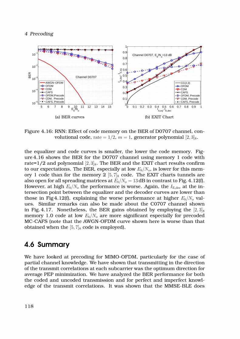
4 Precoding
5 6 7 8 9 10 11 12 13 14 1510
−5
10−4
10−3
10−2
10−1
Eb/N
o
BE
R
Channel D0707
AWGN−OFDMOFDMCDMCAFSOFDM,PrecodeCDM, PrecodeCAFS, Precode
(a) BER curves
0 0.1 0.2 0.3 0.4 0.5 0.6 0.7 0.8 0.9 10
0.1
0.2
0.3
0.4
0.5
0.6
0.7
0.8
0.9
1
IA,eq
, IE,dec
I A,d
ec, I
E,e
q
Channel D0707, Eb/N
o=13 dB
CC(2,3)OFDMCDMCAFSOFDM, PrecodeCDM, PrecodeCAFS, Precode
(b) EXIT Chart
Figure 4.16: RNN: Effect of code memory on the BER of D0707 channel, con-volutional code, rate = 1/2, m = 1, generator polynomial [2, 3]8.
the equalizer and code curves is smaller, the lower the code memory. Fig-ure 4.16 shows the BER for the D0707 channel using memory 1 code withrate=1/2 and polynomial [2, 3]8. The BER and the EXIT chart results confirmto our expectations. The BER, especially at low Eb/No, is lower for this mem-ory 1 code than for the memory 2 [5, 7]8 code. The EXIT charts tunnels arealso open for all spreading matrices at Eb/No = 13 dB in contrast to Fig. 4.12(f).However, at high Eb/No the performance is worse. Again, the IE,dec at the in-tersection point between the equalizer and the decoder curves are lower thanthose in Fig 4.12(f), explaining the worse performance at higher Eb/No val-ues. Similar remarks can also be made about the C0707 channel shownin Fig. 4.17. Nonetheless, the BER gains obtained by employing the [2, 3]8memory 1.0 code at low Eb/No are more significant especially for precodedMC-CAFS (note that the AWGN-OFDM curve shown here is worse than thatobtained when the [5, 7]8 code is employed).
4.6 Summary
We have looked at precoding for MIMO-OFDM, particularly for the case ofpartial channel knowledge. We have shown that transmitting in the directionof the transmit correlations at each subcarrier was the optimum direction foraverage PEP minimization. We have analyzed the BER performance for boththe coded and uncoded transmission and for perfect and imperfect knowl-edge of the transmit correlations. It was shown that the MMSE-BLE does
118
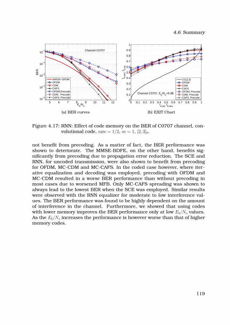
4.6 Summary
5 6 7 8 9 10 11 1210
−5
10−4
10−3
10−2
10−1
Eb/N
o
BE
R
Channel C0707
AWGN−OFDMOFDMCDMCAFSOFDM,PrecodeCDM, PrecodeCAFS, Precode
(a) BER curves
0 0.1 0.2 0.3 0.4 0.5 0.6 0.7 0.8 0.9 10
0.1
0.2
0.3
0.4
0.5
0.6
0.7
0.8
0.9
1
IA,eq
, IE,dec
I A,d
ec, I
E,e
q
Channel C0707, Eb/N
o=9 dB
CC(2,3)OFDMCDMCAFSOFDM, PrecodeCDM, PrecodeCAFS, Precode
(b) EXIT Chart
Figure 4.17: RNN: Effect of code memory on the BER of C0707 channel, con-volutional code, rate = 1/2, m = 1, [2, 3]8.
not benefit from precoding. As a matter of fact, the BER performance wasshown to deteriorate. The MMSE-BDFE, on the other hand, benefits sig-nificantly from precoding due to propagation error reduction. The SCE andRNN, for uncoded transmission, were also shown to benefit from precodingfor OFDM, MC-CDM and MC-CAFS. In the coded case however, where iter-ative equalization and decoding was employed, precoding with OFDM andMC-CDM resulted in a worse BER performance than without precoding inmost cases due to worsened MFB. Only MC-CAFS spreading was shown toalways lead to the lowest BER when the SCE was employed. Similar resultswere observed with the RNN equalizer for moderate to low interference val-ues. The BER performance was found to be highly dependent on the amountof interference in the channel. Furthermore, we showed that using codeswith lower memory improves the BER performance only at low Eb/No values.As the Eb/No increases the performance is however worse than that of highermemory codes.
119
4 Precoding
4.A Appendix to Chapter 4
4.A.1 Antenna Correlations in Frequency Domain
For the sake of clarity, we derive the expression for kTave
for a 2 × 2 MIMOsystem with L = 2. However, the following derivations can be easily extendedto any nT × nR MIMO system with any number of uncorrelated channel tapsL. Accordingly, the 2 × 2 correlation matrices at each channel tap, l, with|ρl| ≤ 1
k(l) =
[
1 ρl
ρ∗l 1
]
=
[
el l
∗l el
] [
el l
l∗ el
]
(4.39)
where el ∈ R, ρl ∈ C, l ∈ C, e2l + |l|2 = 1 and 2ell = ρl.
We shall only consider transmit correlations, but the same derivations canbe applied to obtain the receive k
Rave. The channel matrices at each tap, l
are,
hc(l) =
[
h11(l) h12(l)h21(l) h22(l)
] [
el l
∗l el
]
, (4.40)
Without lost of generality, we shall only consider the first subcarrier fre-quency, k = 1. Thus, we start by calculating the transmit correlation in thefrequency domain at frequency k = 1 as follows
kk
=1
nR
E{HcH
kHc
k} =
1
nR
E{HcH
1Hc
1}, (4.41)
where, using the discrete Fourier transform, the channel transfer functionsat k = 1 are given by,
Hc
1=
[
hc11(1) + hc
11(2) hc12(1) + hc
12(2)hc
21(1) + hc21(2) hc
22(1) + hc22(2)
]
=
[
Hc11 Hc
12
Hc21 Hc
22
]
. (4.42)
Accordingly
HcH
1Hc
1=
[
|Hc11|2 + |Hc
21|2 Hc∗11H
c12 + Hc∗
21Hc22
Hc11H
c∗12 + Hc
21Hc∗22 |Hc
12|2 + |Hc22|2
]
, (4.43)
Similar to the derivation in Appendix 3.A.1, and assuming equal PDP for thechannel taps (E{|hij(l)|2} = 1/L), we can calculate the expected value of diag-onal elements of the above matrix, as follows,
E{|Hc11|2} = E{e2
1|h11(1)|2 + |1|2 |h12(1)|2 + e22|h11(2)|2 + |2|2 |h12(2)|2} = 1.0, (4.44)
and
E{|Hc11|2} = E{|Hc
12|2} = E{|Hc21|2} = E{|Hc
22|2} = 1.0, (4.45)
120
4.A Appendix to Chapter 4
and the off diagonal elements,
E{H∗c11H
c12} = E{e11|h11(1)|2 + e11|h12(1)|2 + e22|h11(2)|2 + e22|h12(2)|2}
=1
2(ρ1 + ρ2) =
1
L
L∑
l=1
ρl, (4.46)
andE{Hc∗
11Hc12} = E{Hc∗
21Hc22} (4.47)
Subsituting the above two equations in Eqn. 4.41, we get
k1
=
[
1 1L
∑Ll=1 ρl
1L
∑Ll=1 ρ∗
l 1
]
=1
L
L∑
l=1
k(l). (4.48)
The above derivation can also be repeated for any frequency k, however theresult does not change, that is
kk
= k1
= kTave
(4.49)
Thus, we can still express KT
as follows,
KTave
= kTave
⊗ IN
. (4.50)
In case of non-equal PDP (E{|hij(l)|2} = σ2l ),
kTave
=
[
1∑L
l=1 σ2l ρl
∑Ll=1 σ2
l ρ∗l 1
]
, (4.51)
where σ2l is the power in the lth MIMO channel tap, and
∑Ll=1 σ2
l = 1.0.
4.A.2 BER curves and EXIT-Charts
BER curves and EXIT-charts for:- A0303, B0303, C0303 and D0303- A0700 and B0700- A0707 and B0707in Table 4.2 for RNN and SCE equalizers and convolutional code withrate=1/2, memory 2 and generator polynomial [7, 5]8.
121
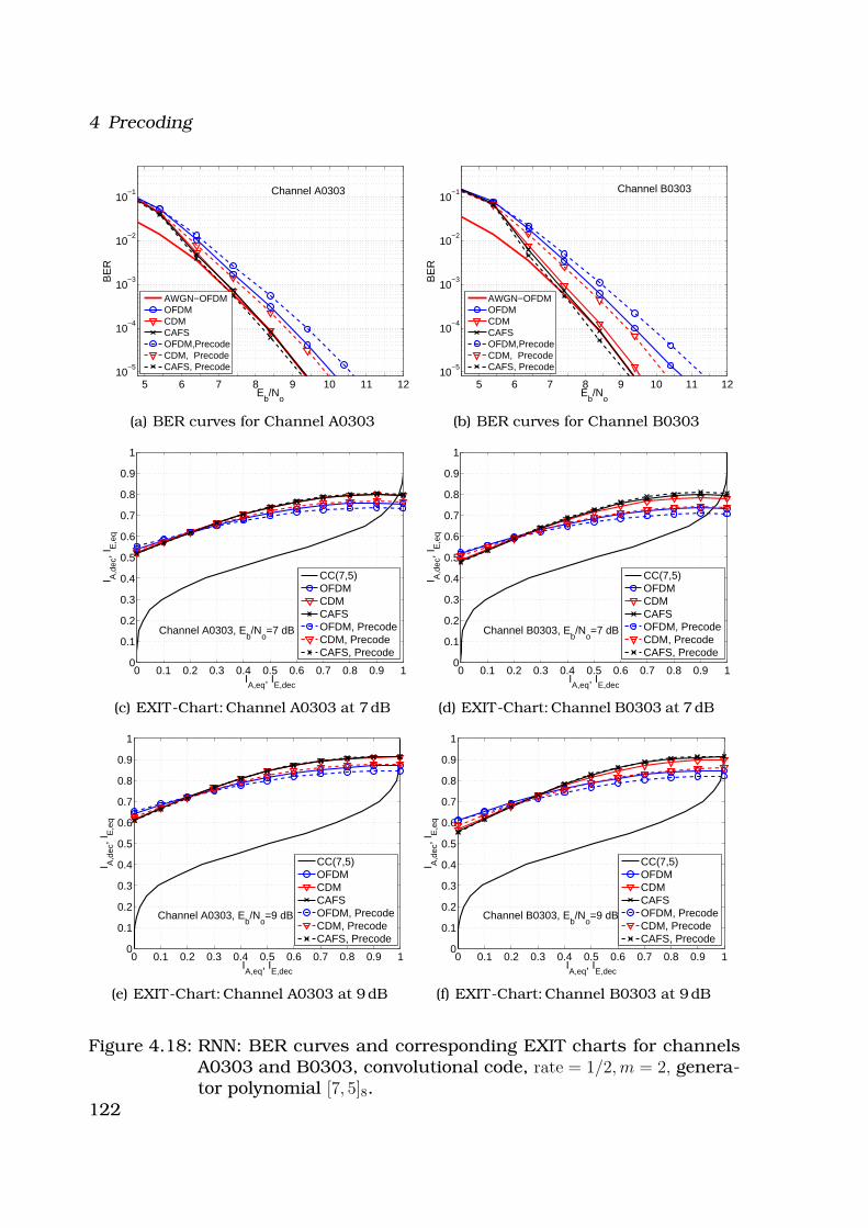
4 Precoding
5 6 7 8 9 10 11 1210
−5
10−4
10−3
10−2
10−1
Eb/N
o
BE
R
Channel A0303
AWGN−OFDMOFDMCDMCAFSOFDM,PrecodeCDM, PrecodeCAFS, Precode
(a) BER curves for Channel A0303
5 6 7 8 9 10 11 1210
−5
10−4
10−3
10−2
10−1
Eb/N
o
BE
R
Channel B0303
AWGN−OFDMOFDMCDMCAFSOFDM,PrecodeCDM, PrecodeCAFS, Precode
(b) BER curves for Channel B0303
0 0.1 0.2 0.3 0.4 0.5 0.6 0.7 0.8 0.9 10
0.1
0.2
0.3
0.4
0.5
0.6
0.7
0.8
0.9
1
IA,eq
, IE,dec
I A,d
ec, I
E,e
q
Channel A0303, Eb/N
o=7 dB
CC(7,5)OFDMCDMCAFSOFDM, PrecodeCDM, PrecodeCAFS, Precode
(c) EXIT-Chart: Channel A0303 at 7 dB
0 0.1 0.2 0.3 0.4 0.5 0.6 0.7 0.8 0.9 10
0.1
0.2
0.3
0.4
0.5
0.6
0.7
0.8
0.9
1
IA,eq
, IE,dec
I A,d
ec, I
E,e
q
Channel B0303, Eb/N
o=7 dB
CC(7,5)OFDMCDMCAFSOFDM, PrecodeCDM, PrecodeCAFS, Precode
(d) EXIT-Chart: Channel B0303 at 7 dB
0 0.1 0.2 0.3 0.4 0.5 0.6 0.7 0.8 0.9 10
0.1
0.2
0.3
0.4
0.5
0.6
0.7
0.8
0.9
1
IA,eq
, IE,dec
I A,d
ec, I
E,e
q
Channel A0303, Eb/N
o=9 dB
CC(7,5)OFDMCDMCAFSOFDM, PrecodeCDM, PrecodeCAFS, Precode
(e) EXIT-Chart: Channel A0303 at 9 dB
0 0.1 0.2 0.3 0.4 0.5 0.6 0.7 0.8 0.9 10
0.1
0.2
0.3
0.4
0.5
0.6
0.7
0.8
0.9
1
IA,eq
, IE,dec
I A,d
ec, I
E,e
q
Channel B0303, Eb/N
o=9 dB
CC(7,5)OFDMCDMCAFSOFDM, PrecodeCDM, PrecodeCAFS, Precode
(f) EXIT-Chart: Channel B0303 at 9 dB
Figure 4.18: RNN: BER curves and corresponding EXIT charts for channelsA0303 and B0303, convolutional code, rate = 1/2,m = 2, genera-tor polynomial [7, 5]8.
122
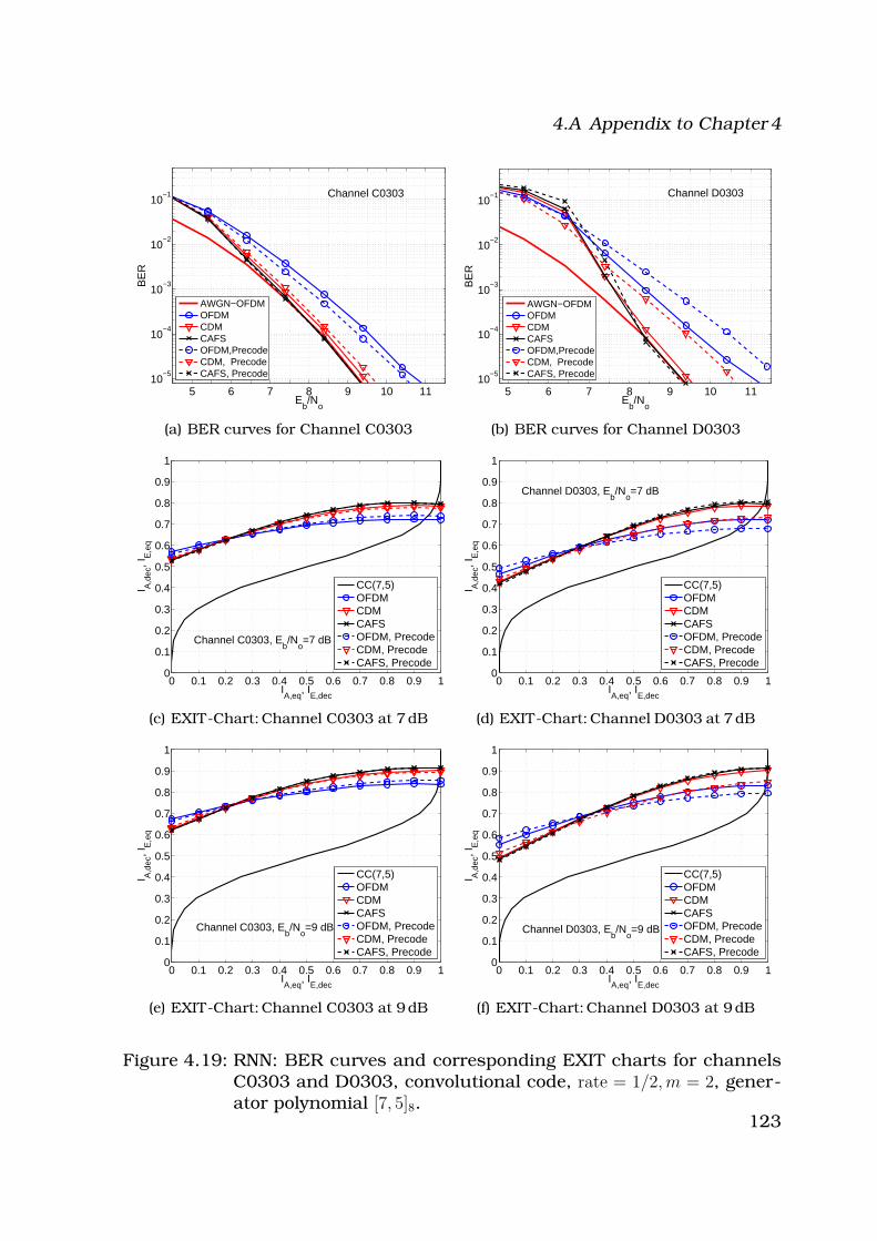
4.A Appendix to Chapter 4
5 6 7 8 9 10 1110
−5
10−4
10−3
10−2
10−1
Eb/N
o
BE
R
Channel C0303
AWGN−OFDMOFDMCDMCAFSOFDM,PrecodeCDM, PrecodeCAFS, Precode
(a) BER curves for Channel C0303
5 6 7 8 9 10 1110
−5
10−4
10−3
10−2
10−1
Eb/N
o
BE
R
Channel D0303
AWGN−OFDMOFDMCDMCAFSOFDM,PrecodeCDM, PrecodeCAFS, Precode
(b) BER curves for Channel D0303
0 0.1 0.2 0.3 0.4 0.5 0.6 0.7 0.8 0.9 10
0.1
0.2
0.3
0.4
0.5
0.6
0.7
0.8
0.9
1
IA,eq
, IE,dec
I A,d
ec, I
E,e
q
Channel C0303, Eb/N
o=7 dB
CC(7,5)OFDMCDMCAFSOFDM, PrecodeCDM, PrecodeCAFS, Precode
(c) EXIT-Chart: Channel C0303 at 7 dB
0 0.1 0.2 0.3 0.4 0.5 0.6 0.7 0.8 0.9 10
0.1
0.2
0.3
0.4
0.5
0.6
0.7
0.8
0.9
1
IA,eq
, IE,dec
I A,d
ec, I
E,e
q
Channel D0303, Eb/N
o=7 dB
CC(7,5)OFDMCDMCAFSOFDM, PrecodeCDM, PrecodeCAFS, Precode
(d) EXIT-Chart: Channel D0303 at 7 dB
0 0.1 0.2 0.3 0.4 0.5 0.6 0.7 0.8 0.9 10
0.1
0.2
0.3
0.4
0.5
0.6
0.7
0.8
0.9
1
IA,eq
, IE,dec
I A,d
ec, I
E,e
q
Channel C0303, Eb/N
o=9 dB
CC(7,5)OFDMCDMCAFSOFDM, PrecodeCDM, PrecodeCAFS, Precode
(e) EXIT-Chart: Channel C0303 at 9 dB
0 0.1 0.2 0.3 0.4 0.5 0.6 0.7 0.8 0.9 10
0.1
0.2
0.3
0.4
0.5
0.6
0.7
0.8
0.9
1
IA,eq
, IE,dec
I A,d
ec, I
E,e
q
Channel D0303, Eb/N
o=9 dB
CC(7,5)OFDMCDMCAFSOFDM, PrecodeCDM, PrecodeCAFS, Precode
(f) EXIT-Chart: Channel D0303 at 9 dB
Figure 4.19: RNN: BER curves and corresponding EXIT charts for channelsC0303 and D0303, convolutional code, rate = 1/2,m = 2, gener-ator polynomial [7, 5]8.
123

4 Precoding
6 7 8 9 10 1110
−5
10−4
10−3
10−2
10−1
Eb/N
o
BE
R
Channel A0700
AWGN−OFDMOFDMCDMCAFSOFDM,PrecodeCDM, PrecodeCAFS, Precode
(a) BER curves for Channel A0700
5 6 7 8 9 10 1110
−5
10−4
10−3
10−2
10−1
Eb/N
o
BE
R
Channel B0700
AWGN−OFDMOFDMCDMCAFSOFDM,PrecodeCDM, PrecodeCAFS, Precode
(b) BER curves for Channel B0700
0 0.1 0.2 0.3 0.4 0.5 0.6 0.7 0.8 0.9 10
0.1
0.2
0.3
0.4
0.5
0.6
0.7
0.8
0.9
1
IA,eq
, IE,dec
I A,d
ec, I
E,e
q
Channel A0700, Eb/N
o=7 dB
CC(7,5)OFDMCDMCAFSOFDM, PrecodeCDM, PrecodeCAFS, Precode
(c) EXIT-Chart: Channel A0700 at 7 dB
0 0.1 0.2 0.3 0.4 0.5 0.6 0.7 0.8 0.9 10
0.1
0.2
0.3
0.4
0.5
0.6
0.7
0.8
0.9
1
IA,eq
, IE,dec
I A,d
ec, I
E,e
q
Channel B0700, Eb/N
o=7 dB
CC(7,5)OFDMCDMCAFSOFDM, PrecodeCDM, PrecodeCAFS, Precode
(d) EXIT-Chart: Channel B0700 at 7 dB
0 0.1 0.2 0.3 0.4 0.5 0.6 0.7 0.8 0.9 10
0.1
0.2
0.3
0.4
0.5
0.6
0.7
0.8
0.9
1
IA,eq
, IE,dec
I A,d
ec, I
E,e
q
Channel A0700, Eb/N
o=9 dB
CC(7,5)OFDMCDMCAFSOFDM, PrecodeCDM, PrecodeCAFS, Precode
(e) EXIT-Chart: Channel A0700 at 9 dB
0 0.1 0.2 0.3 0.4 0.5 0.6 0.7 0.8 0.9 10
0.1
0.2
0.3
0.4
0.5
0.6
0.7
0.8
0.9
1
IA,eq
, IE,dec
I A,d
ec, I
E,e
q
Channel B0700, Eb/N
o=9 dB
CC(7,5)OFDMCDMCAFSOFDM, PrecodeCDM, PrecodeCAFS, Precode
(f) EXIT-Chart: Channel B0700 at 9 dB
Figure 4.20: RNN: BER curves and corresponding EXIT charts for channelsA0700 and B0700, convolutional code, rate = 1/2,m = 2, genera-tor polynomial [7, 5]8.
124
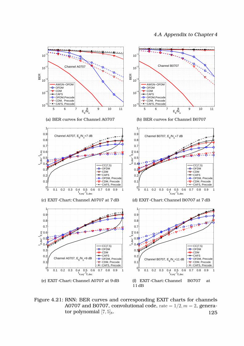
4.A Appendix to Chapter 4
5 6 7 8 9 10 1110
−5
10−4
10−3
10−2
10−1
Eb/N
o
BE
R
Channel A0707
AWGN−OFDMOFDMCDMCAFSOFDM,PrecodeCDM, PrecodeCAFS, Precode
(a) BER curves for Channel A0707
5 6 7 8 9 10 1110
−5
10−4
10−3
10−2
10−1
Eb/N
o
BE
R
Channel B0707
AWGN−OFDMOFDMCDMCAFSOFDM,PrecodeCDM, PrecodeCAFS, Precode
(b) BER curves for Channel B0707
0 0.1 0.2 0.3 0.4 0.5 0.6 0.7 0.8 0.9 10
0.1
0.2
0.3
0.4
0.5
0.6
0.7
0.8
0.9
1
IA,eq
, IE,dec
I A,d
ec, I
E,e
q
Channel A0707, Eb/N
o=7 dB
CC(7,5)OFDMCDMCAFSOFDM, PrecodeCDM, PrecodeCAFS, Precode
(c) EXIT-Chart: Channel A0707 at 7 dB
0 0.1 0.2 0.3 0.4 0.5 0.6 0.7 0.8 0.9 10
0.1
0.2
0.3
0.4
0.5
0.6
0.7
0.8
0.9
1
IA,eq
, IE,dec
I A,d
ec, I
E,e
q
Channel B0707, Eb/N
o=7 dB
CC(7,5)OFDMCDMCAFSOFDM, PrecodeCDM, PrecodeCAFS, Precode
(d) EXIT-Chart: Channel B0707 at 7 dB
0 0.1 0.2 0.3 0.4 0.5 0.6 0.7 0.8 0.9 10
0.1
0.2
0.3
0.4
0.5
0.6
0.7
0.8
0.9
1
IA,eq
, IE,dec
I A,d
ec, I
E,e
q
Channel A0707, Eb/N
o=9 dB
CC(7,5)OFDMCDMCAFSOFDM, PrecodeCDM, PrecodeCAFS, Precode
(e) EXIT-Chart: Channel A0707 at 9 dB
0 0.1 0.2 0.3 0.4 0.5 0.6 0.7 0.8 0.9 10
0.1
0.2
0.3
0.4
0.5
0.6
0.7
0.8
0.9
1
IA,eq
, IE,dec
I A,d
ec, I
E,e
q
Channel B0707, Eb/N
o=11 dB
CC(7,5)OFDMCDMCAFSOFDM, PrecodeCDM, PrecodeCAFS, Precode
(f) EXIT-Chart: Channel B0707 at11 dB
Figure 4.21: RNN: BER curves and corresponding EXIT charts for channelsA0707 and B0707, convolutional code, rate = 1/2,m = 2, genera-tor polynomial [7, 5]8. 125
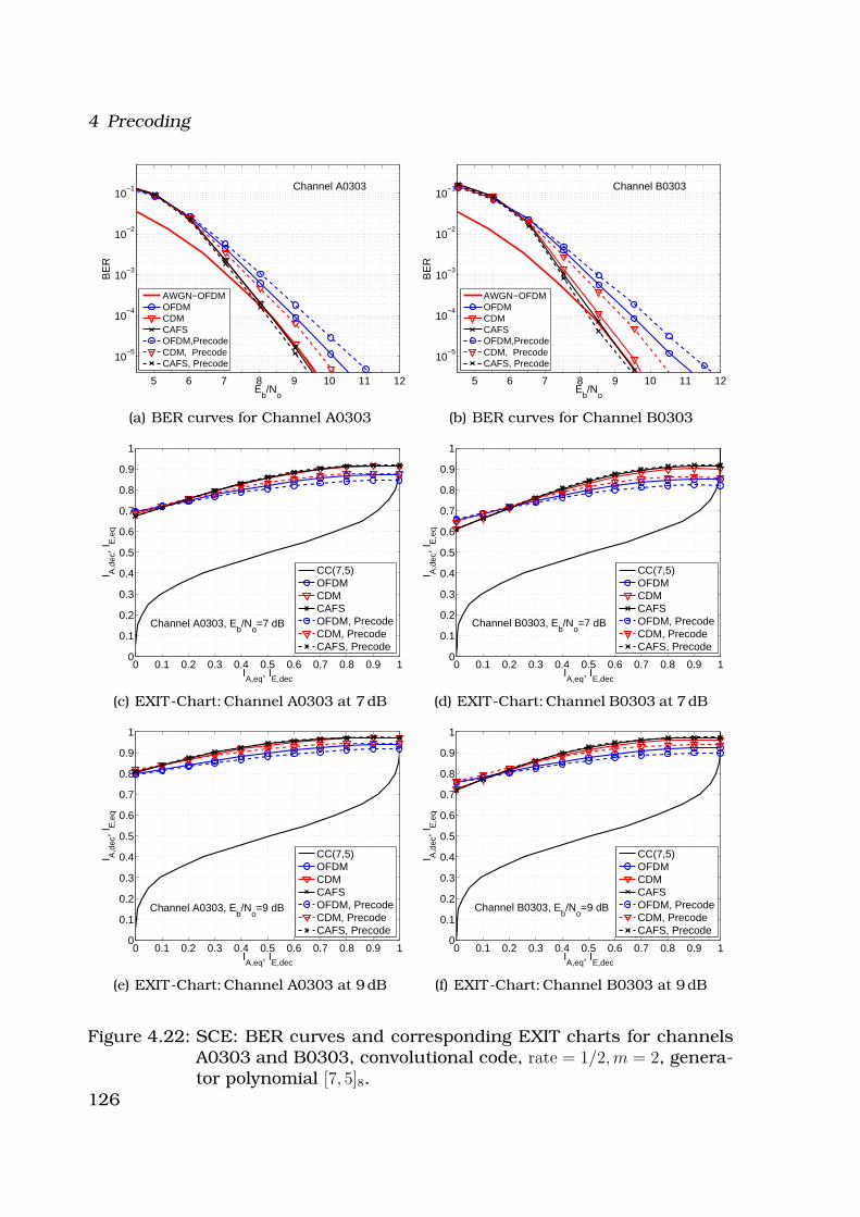
4 Precoding
5 6 7 8 9 10 11 12
10−5
10−4
10−3
10−2
10−1
Eb/N
o
BE
R
Channel A0303
AWGN−OFDMOFDMCDMCAFSOFDM,PrecodeCDM, PrecodeCAFS, Precode
(a) BER curves for Channel A0303
5 6 7 8 9 10 11 12
10−5
10−4
10−3
10−2
10−1
Eb/N
o
BE
R
Channel B0303
AWGN−OFDMOFDMCDMCAFSOFDM,PrecodeCDM, PrecodeCAFS, Precode
(b) BER curves for Channel B0303
0 0.1 0.2 0.3 0.4 0.5 0.6 0.7 0.8 0.9 10
0.1
0.2
0.3
0.4
0.5
0.6
0.7
0.8
0.9
1
IA,eq
, IE,dec
I A,d
ec, I
E,e
q
Channel A0303, Eb/N
o=7 dB
CC(7,5)OFDMCDMCAFSOFDM, PrecodeCDM, PrecodeCAFS, Precode
(c) EXIT-Chart: Channel A0303 at 7 dB
0 0.1 0.2 0.3 0.4 0.5 0.6 0.7 0.8 0.9 10
0.1
0.2
0.3
0.4
0.5
0.6
0.7
0.8
0.9
1
IA,eq
, IE,dec
I A,d
ec, I
E,e
q
Channel B0303, Eb/N
o=7 dB
CC(7,5)OFDMCDMCAFSOFDM, PrecodeCDM, PrecodeCAFS, Precode
(d) EXIT-Chart: Channel B0303 at 7 dB
0 0.1 0.2 0.3 0.4 0.5 0.6 0.7 0.8 0.9 10
0.1
0.2
0.3
0.4
0.5
0.6
0.7
0.8
0.9
1
IA,eq
, IE,dec
I A,d
ec, I
E,e
q
Channel A0303, Eb/N
o=9 dB
CC(7,5)OFDMCDMCAFSOFDM, PrecodeCDM, PrecodeCAFS, Precode
(e) EXIT-Chart: Channel A0303 at 9 dB
0 0.1 0.2 0.3 0.4 0.5 0.6 0.7 0.8 0.9 10
0.1
0.2
0.3
0.4
0.5
0.6
0.7
0.8
0.9
1
IA,eq
, IE,dec
I A,d
ec, I
E,e
q
Channel B0303, Eb/N
o=9 dB
CC(7,5)OFDMCDMCAFSOFDM, PrecodeCDM, PrecodeCAFS, Precode
(f) EXIT-Chart: Channel B0303 at 9 dB
Figure 4.22: SCE: BER curves and corresponding EXIT charts for channelsA0303 and B0303, convolutional code, rate = 1/2,m = 2, genera-tor polynomial [7, 5]8.
126

4.A Appendix to Chapter 4
4 5 6 7 8 9 10 11 12
10−5
10−4
10−3
10−2
10−1
Eb/N
o
BE
R
Channel C0303
AWGN−OFDMOFDMCDMCAFSOFDM,PrecodeCDM, PrecodeCAFS, Precode
(a) BER curves for Channel C0303
5 6 7 8 9 10 11 12
10−5
10−4
10−3
10−2
10−1
Eb/N
o
BE
R
Channel D0303
AWGN−OFDMOFDMCDMCAFSOFDM,PrecodeCDM, PrecodeCAFS, Precode
(b) BER curves for Channel D0303
0 0.1 0.2 0.3 0.4 0.5 0.6 0.7 0.8 0.9 10
0.1
0.2
0.3
0.4
0.5
0.6
0.7
0.8
0.9
1
IA,eq
, IE,dec
I A,d
ec, I
E,e
q
Channel C0303, Eb/N
o=7 dB
CC(7,5)OFDMCDMCAFSOFDM, PrecodeCDM, PrecodeCAFS, Precode
(c) EXIT-Chart: Channel C0303 at 7 dB
0 0.1 0.2 0.3 0.4 0.5 0.6 0.7 0.8 0.9 10
0.1
0.2
0.3
0.4
0.5
0.6
0.7
0.8
0.9
1
IA,eq
, IE,dec
I A,d
ec, I
E,e
q
Channel D0303, Eb/N
o=7 dB
CC(7,5)OFDMCDMCAFSOFDM, PrecodeCDM, PrecodeCAFS, Precode
(d) EXIT-Chart: Channel D0303 at 7 dB
0 0.1 0.2 0.3 0.4 0.5 0.6 0.7 0.8 0.9 10
0.1
0.2
0.3
0.4
0.5
0.6
0.7
0.8
0.9
1
IA,eq
, IE,dec
I A,d
ec, I
E,e
q
Channel C0303, Eb/N
o=9 dB
CC(7,5)OFDMCDMCAFSOFDM, PrecodeCDM, PrecodeCAFS, Precode
(e) EXIT-Chart: Channel C0303 at 9 dB
0 0.1 0.2 0.3 0.4 0.5 0.6 0.7 0.8 0.9 10
0.1
0.2
0.3
0.4
0.5
0.6
0.7
0.8
0.9
1
IA,eq
, IE,dec
I A,d
ec, I
E,e
q
Channel D0303, Eb/N
o=9 dB
CC(7,5)OFDMCDMCAFSOFDM, PrecodeCDM, PrecodeCAFS, Precode
(f) EXIT-Chart: Channel D0303 at 9 dB
Figure 4.23: SCE: BER curves and corresponding EXIT charts for channelsC0303 and D0303, convolutional code, rate = 1/2,m = 2, gener-ator polynomial [7, 5]8.
127
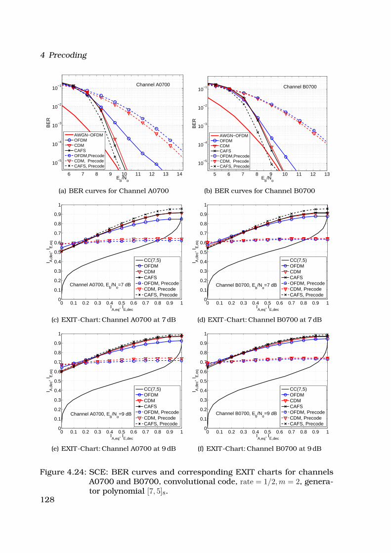
4 Precoding
6 7 8 9 10 11 12 13 14
10−5
10−4
10−3
10−2
10−1
Eb/N
o
BE
R
Channel A0700
AWGN−OFDMOFDMCDMCAFSOFDM,PrecodeCDM, PrecodeCAFS, Precode
(a) BER curves for Channel A0700
5 6 7 8 9 10 11 12 13
10−5
10−4
10−3
10−2
10−1
Eb/N
o
BE
R
Channel B0700
AWGN−OFDMOFDMCDMCAFSOFDM,PrecodeCDM, PrecodeCAFS, Precode
(b) BER curves for Channel B0700
0 0.1 0.2 0.3 0.4 0.5 0.6 0.7 0.8 0.9 10
0.1
0.2
0.3
0.4
0.5
0.6
0.7
0.8
0.9
1
IA,eq
, IE,dec
I A,d
ec, I
E,e
q
Channel A0700, Eb/N
o=7 dB
CC(7,5)OFDMCDMCAFSOFDM, PrecodeCDM, PrecodeCAFS, Precode
(c) EXIT-Chart: Channel A0700 at 7 dB
0 0.1 0.2 0.3 0.4 0.5 0.6 0.7 0.8 0.9 10
0.1
0.2
0.3
0.4
0.5
0.6
0.7
0.8
0.9
1
IA,eq
, IE,dec
I A,d
ec, I
E,e
q
Channel B0700, Eb/N
o=7 dB
CC(7,5)OFDMCDMCAFSOFDM, PrecodeCDM, PrecodeCAFS, Precode
(d) EXIT-Chart: Channel B0700 at 7 dB
0 0.1 0.2 0.3 0.4 0.5 0.6 0.7 0.8 0.9 10
0.1
0.2
0.3
0.4
0.5
0.6
0.7
0.8
0.9
1
IA,eq
, IE,dec
I A,d
ec, I
E,e
q
Channel A0700, Eb/N
o=9 dB
CC(7,5)OFDMCDMCAFSOFDM, PrecodeCDM, PrecodeCAFS, Precode
(e) EXIT-Chart: Channel A0700 at 9 dB
0 0.1 0.2 0.3 0.4 0.5 0.6 0.7 0.8 0.9 10
0.1
0.2
0.3
0.4
0.5
0.6
0.7
0.8
0.9
1
IA,eq
, IE,dec
I A,d
ec, I
E,e
q
Channel B0700, Eb/N
o=9 dB
CC(7,5)OFDMCDMCAFSOFDM, PrecodeCDM, PrecodeCAFS, Precode
(f) EXIT-Chart: Channel B0700 at 9 dB
Figure 4.24: SCE: BER curves and corresponding EXIT charts for channelsA0700 and B0700, convolutional code, rate = 1/2,m = 2, genera-tor polynomial [7, 5]8.
128
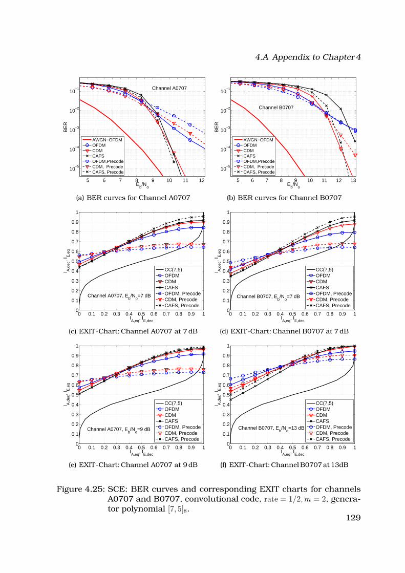
4.A Appendix to Chapter 4
5 6 7 8 9 10 11 12
10−5
10−4
10−3
10−2
10−1
Eb/N
o
BE
R
Channel A0707
AWGN−OFDMOFDMCDMCAFSOFDM,PrecodeCDM, PrecodeCAFS, Precode
(a) BER curves for Channel A0707
5 6 7 8 9 10 11 12 13
10−5
10−4
10−3
10−2
10−1
Eb/N
o
BE
R
Channel B0707
AWGN−OFDMOFDMCDMCAFSOFDM,PrecodeCDM, PrecodeCAFS, Precode
(b) BER curves for Channel B0707
0 0.1 0.2 0.3 0.4 0.5 0.6 0.7 0.8 0.9 10
0.1
0.2
0.3
0.4
0.5
0.6
0.7
0.8
0.9
1
IA,eq
, IE,dec
I A,d
ec, I
E,e
q
Channel A0707, Eb/N
o=7 dB
CC(7,5)OFDMCDMCAFSOFDM, PrecodeCDM, PrecodeCAFS, Precode
(c) EXIT-Chart: Channel A0707 at 7 dB
0 0.1 0.2 0.3 0.4 0.5 0.6 0.7 0.8 0.9 10
0.1
0.2
0.3
0.4
0.5
0.6
0.7
0.8
0.9
1
IA,eq
, IE,dec
I A,d
ec, I
E,e
q
Channel B0707, Eb/N
o=7 dB
CC(7,5)OFDMCDMCAFSOFDM, PrecodeCDM, PrecodeCAFS, Precode
(d) EXIT-Chart: Channel B0707 at 7 dB
0 0.1 0.2 0.3 0.4 0.5 0.6 0.7 0.8 0.9 10
0.1
0.2
0.3
0.4
0.5
0.6
0.7
0.8
0.9
1
IA,eq
, IE,dec
I A,d
ec, I
E,e
q
Channel A0707, Eb/N
o=9 dB
CC(7,5)OFDMCDMCAFSOFDM, PrecodeCDM, PrecodeCAFS, Precode
(e) EXIT-Chart: Channel A0707 at 9 dB
0 0.1 0.2 0.3 0.4 0.5 0.6 0.7 0.8 0.9 10
0.1
0.2
0.3
0.4
0.5
0.6
0.7
0.8
0.9
1
IA,eq
, IE,dec
I A,d
ec, I
E,e
q
Channel B0707, Eb/N
o=13 dB
CC(7,5)OFDMCDMCAFSOFDM, PrecodeCDM, PrecodeCAFS, Precode
(f) EXIT-Chart: Channel B0707 at 13dB
Figure 4.25: SCE: BER curves and corresponding EXIT charts for channelsA0707 and B0707, convolutional code, rate = 1/2,m = 2, genera-tor polynomial [7, 5]8.
129

4 Precoding
130

Chapter5MIMO Channel Capacity: Theoryversus Measurement
In this chapter, we look at the capacity and correlations of measured MIMOchannels for a specific outdoor scenario. We first start by giving a theoret-ical overview of MIMO channel capacity for both flat fading and frequencyselective channels in presence of no, partial or full channel knowledge at thetransmitter. We then describe the measurement setup and give the corre-sponding channel capacities and antenna correlations. The calculated ca-pacity of the measured MIMO channels is compared with that of theoreticalmodels.
5.1 MIMO Channel Capacity
In this section, we give the capacity for flat fading MIMO. The expression forthe MIMO channel capacity was first introduced in [1]. The author differenti-ated between deterministic channels (channel state information is present atthe transmitter CSIT) and randomly changing channels (Channel unknown
131
5 MIMO Channel Capacity: Theory versus Measurement
to the transmitter). As mentioned in the previous chapter, although full chan-nel knowledge is not always available at the transmitter, partial knowledge(e. g. fading correlations) is more readily available and can be utilized by thetransmitter. In what follows, we thus present the MIMO channel capacityfor three cases: no channel knowledge, full channel knowledge and partialchannel knowledge at the transmitter. We always assume that the channelis known to the receiver.
5.1.1 No channel knowledge at the transmitter
The capacity of any channel can be calculated either in the frequency or thetime domain. We first look at the capacity of a flat fading random channel inthe time domain. In this case, the MIMO ergodic (mean) channel capacity isgiven by [1, 4]
CR = E{log2 det(InR
+P
NonT
hQhH)} = E{log2 det(InR
+ρo
nT
hhH)}, (5.1)
where h is the channel matrix in the time domain and the expectation is takenover all channel realizations, P is the total transmit power, No is the noisepower, and thus ρo = P/No is the signal to noise ratio (SNR). The covariancematrix of the transmit signals, Q, is given by
Q = InT
. (5.2)
That is, the total transmit power is distributed equally over all transmit an-tennas nT. It is important to mention here that this is not the Shannoncapacity in the true sense, since, as shown next, in presence of full channelknowledge a signal covariance matrix can be chosen that outperforms thatin Eqn. 5.2 [22]. Nonetheless, as is customarily done in the literature, weshall still refer to Eqn. 5.1 as the channel capacity. Equation 5.1 can also bewritten in terms of the channel singular values, λi, (i. e. the eigenvalues ofhhH ) as follows [1, 4, 3]
CR = E{log2 det(InR
+ρo
nT
hhH)} = E{r∑
i=1
log2(1 +ρo
nT
λi)}, (5.3)
where r is the rank of h.
As mentioned above, the channel capacity can be equivalently calculatedin the frequency domain. For a frequency selective channel, it is easier tocalculate the capacity in the frequency domain. In this case, we can makeuse of the discrete Fourier transform (DFT) [79, 91]. The capacity CR of a
132
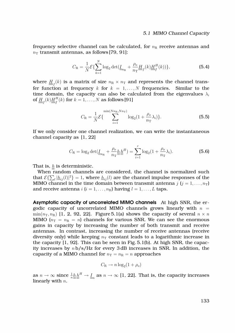
5.1 MIMO Channel Capacity
frequency selective channel can be calculated, for nR receive antennas andnT transmit antennas, as follows [79, 91]:
CR =1
NE{
N∑
k=1
log2 det(InR
+ρo
nT
Hf(k)HH
f(k))}, (5.4)
where Hf(k) is a matrix of size nR × nT and represents the channel trans-
fer function at frequency k for k = 1, . . . , N frequencies. Similar to thetime domain, the capacity can also be calculated from the eigenvalues λi
of Hf(k)HH
f(k) for k = 1, . . . , N as follows [91]
CR =1
NE{
min(NnR,NnT)∑
i=1
log2(1 +ρo
nT
λi)}. (5.5)
If we only consider one channel realization, we can write the instantaneouschannel capacity as [1, 22]
CR = log2 det(InR
+ρo
nT
hhH) =r∑
i=1
log2(1 +ρo
nT
λi). (5.6)
That is, h is deterministic.
When random channels are considered, the channel is normalized suchthat E{∑l |hij(l)|2} = 1, where hij(l) are the channel impulse responses of theMIMO channel in the time domain between transmit antenna j (j = 1, . . . , nT)and receive antenna i (i = 1, . . . , nR) having l = 1, . . . , L taps.
Asymptotic capacity of uncorrelated MIMO channels At high SNR, the er-godic capacity of uncorrelated MIMO channels grows linearly with n =min(nT, nR) [1, 2, 92, 22]. Figure 5.1(a) shows the capacity of several n × nMIMO (nT = nR = n) channels for various SNR. We can see the enormousgains in capacity by increasing the number of both transmit and receiveantennas. In contrast, increasing the number of receive antennas (receivediversity only) while keeping nT constant leads to a logarithmic increase inthe capacity [1, 92]. This can be seen in Fig. 5.1(b). At high SNR, the capac-ity increases by n b/s/Hz for every 3 dB increases in SNR. In addition, thecapacity of a MIMO channel for nT = nR = n approaches
CR → n log2(1 + ρo)
as n → ∞ since 1nhhH → I
nas n → ∞ [1, 22]. That is, the capacity increases
linearly with n.
133
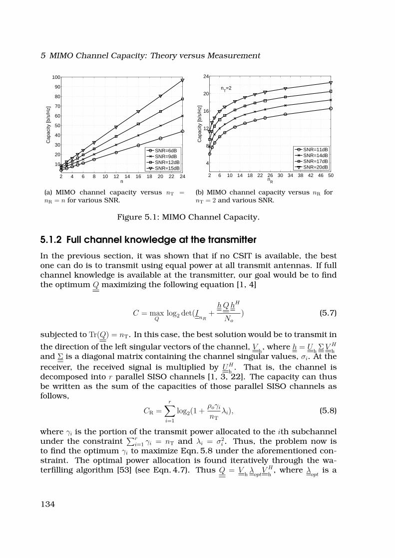
5 MIMO Channel Capacity: Theory versus Measurement
2 4 6 8 10 12 14 16 18 20 22 24
10
20
30
40
50
60
70
80
90
100
n
Cap
acity
[b/s
/Hz]
SNR=6dBSNR=9dBSNR=12dBSNR=15dB
(a) MIMO channel capacity versus nT =nR = n for various SNR.
2 6 10 14 18 22 26 30 34 38 42 46 50
4
8
12
16
20
24
nR
Cap
acity
[b/s
/Hz]
nT=2
SNR=11dBSNR=14dBSNR=17dBSNR=20dB
(b) MIMO channel capacity versus nR fornT = 2 and various SNR.
Figure 5.1: MIMO Channel Capacity.
5.1.2 Full channel knowledge at the transmitter
In the previous section, it was shown that if no CSIT is available, the bestone can do is to transmit using equal power at all transmit antennas. If fullchannel knowledge is available at the transmitter, our goal would be to findthe optimum Q maximizing the following equation [1, 4]
C = maxQ
log2 det(InR
+hQhH
No
) (5.7)
subjected to Tr(Q) = nT. In this case, the best solution would be to transmit in
the direction of the left singular vectors of the channel, Vh, where h = U
hΣ V H
hand Σ is a diagonal matrix containing the channel singular values, σi. At the
receiver, the received signal is multiplied by UH
h. That is, the channel is
decomposed into r parallel SISO channels [1, 3, 22]. The capacity can thusbe written as the sum of the capacities of those parallel SISO channels asfollows,
CR =r∑
i=1
log2(1 +ρoγi
nT
λi), (5.8)
where γi is the portion of the transmit power allocated to the ith subchannelunder the constraint
∑ri=1 γi = nT and λi = σ2
i . Thus, the problem now isto find the optimum γi to maximize Eqn. 5.8 under the aforementioned con-straint. The optimal power allocation is found iteratively through the wa-terfilling algorithm [53] (see Eqn. 4.7). Thus Q = V
hλ
optV H
h, where λ
optis a
134
5.1 MIMO Channel Capacity
diagonal matrix containing the optimum γi values. As mentioned in Sec.4.2depending on the channel eigenvalues and the available transmit power someof the weak modes might receive zero power. If only one eigenmode gets allof the available transmit power (Q is rank 1), we denote this transmission
strategy beamforming [93].
5.1.3 Partial channel knowledge at the transmitter
In the previous sections, we considered the cases of either full or no channelknowledge at the transmitter. Now, we consider the case of partial channelknowledge being available. To be more specific, we also assume that only thetransmit correlation matrix, k
T, is known to the transmitter. In this case, the
channel capacity is given by
C = maxQ
E{log2 det(InR
+H Q HH
No
)}
subjected to Tr(Q) = nT. In this case, the optimum input covariance matrix
is given by [94, 80]Q = v
Tλ
optvH
T,
where kT
= vTeT
vHT
and, as mentioned in Sec. 4.3, the diagonal matrix λopt
is obtained through numerical optimization resembling that of waterfilling,where stronger modes are allocated more power than weaker ones [94, 80].The authors in [82] considered both transmit and receive correlations andhave shown that, although one still needs to transmit in direction of thetransmit correlation eigenvectors, the energy distribution at the transmitteris dependent on both the transmit and receive correlations.
Although numerical power allocation strategies are optimum, transmittingusing less optimum solutions can still lead to results very close to the op-timum ones. In [75], a non optimum power allocation strategy, stochastic
water-filling, was proposed where waterfilling is done on the weighted eigen-values of k
T. This stochastic strategy performs very close to the optimum
power allocation when fading correlations are high.Similarly, for frequency selective channels, it was shown in [21] that trans-
mitting in the direction of the transmit correlations eigenvectors at eachsubcarrier maximizes the capacity. Likewise, the power allocation is donethrough numerical optimization. The authors nonetheless showed that wa-terfilling on the eigenvalues of the transmit correlations, although subopti-mal, leads to almost optimum results.
Figure 5.2 compares the MIMO capacity for correlated fading with that ofuncorrelated fading assuming full, partial or no channel knowledge at the
135
5 MIMO Channel Capacity: Theory versus Measurement
transmitter. For the correlated case, the exponential correlation model isassumed with ρ = 0.9. In case of partial CSIT, the stochastic water-fillingalgorithm was employed. As expected, the presence of antenna correlationscauses a loss in capacity, especially if absolutely no channel knowledge isavailable at the transmitter. Nonetheless, in case of partial CSIT, the channelcapacity using this suboptimum stochastic waterfilling method is seen to lievery close to that of full channel knowledge.
5.1.4 Impact of Antenna Correlations on MIMO Capacity
To closely examine the effect of antenna correlations on the MIMO capacity,we consider the MIMO capacity at high SNR assuming nT = nR = n and k
Tand k
Rto be full rank. The capacity can thus be written as [22]
C ≈ log2 det(ρo
nT
hhH) + log2 det(kT) + log2 det(k
R), (5.9)
where h are the white uncorrelated zero mean complex channel coefficients.Clearly, k
Tand k
Rhave the same effect on the channel capacity. Since the
det(k) =∏
i λi(k) and∑
i λi(k) = n and making use of the inequality of thearithmetic and geometric means, we have
∏
i λi(k) ≤ 1.0. That is, log2(det(k)) ≤0 and is zero only if k = I. Thus, correlations are detrimental to the MIMOcapacity leading to loss in capacity as is also shown in Fig. 5.2.
5.1.5 Impact of Line of Sight on MIMO Capacity
The effect of the line of sight (LOS) component on the MIMO channel capacitycan be examined by considering Rician fading where the channel is modeledas a sum of a LOS matrix and a Rayleigh fading matrix as follows
h =
√
K
1 + Kh +
√
1
1 + Kh
w(5.10)
where h is the fixed component, hw
the Rayleigh component and K the Ricianfactor. K is equal to the ratio of the power in the LOS component to that inthe pure fading channel. K = 0 represents pure Rayleigh fading, and K → ∞represents a non fading channel. The performance of the Rician channel isthus dependent on K as well on the components of the matrix h. Thus, ifK = 0, the capacity reduces to that of a Rayleigh channel. On the other side,if K → ∞, then the capacity is dependent on the structure of h as we shownext.
136
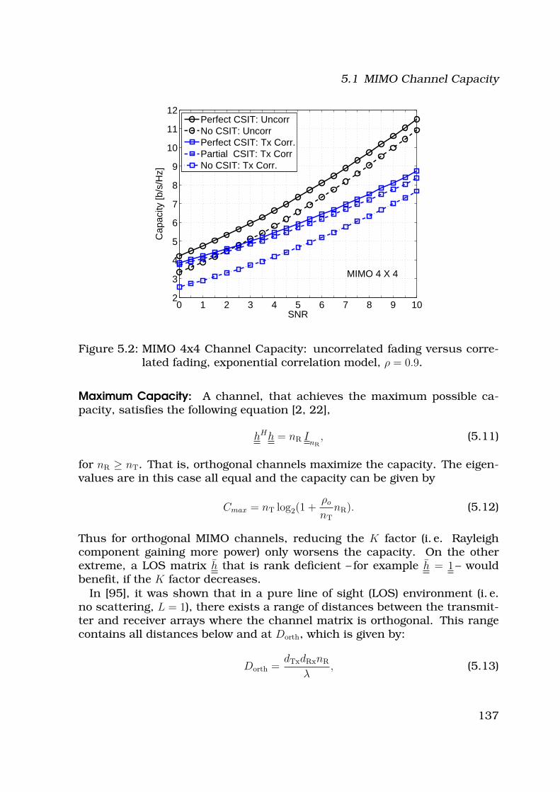
5.1 MIMO Channel Capacity
0 1 2 3 4 5 6 7 8 9 102
3
4
5
6
7
8
9
10
11
12
SNR
Cap
acity
[b/s
/Hz]
MIMO 4 X 4
Perfect CSIT: UncorrNo CSIT: UncorrPerfect CSIT: Tx Corr.Partial CSIT: Tx CorrNo CSIT: Tx Corr.
Figure 5.2: MIMO 4x4 Channel Capacity: uncorrelated fading versus corre-lated fading, exponential correlation model, ρ = 0.9.
Maximum Capacity: A channel, that achieves the maximum possible ca-pacity, satisfies the following equation [2, 22],
hHh = nR InR
, (5.11)
for nR ≥ nT. That is, orthogonal channels maximize the capacity. The eigen-values are in this case all equal and the capacity can be given by
Cmax = nT log2(1 +ρo
nT
nR). (5.12)
Thus for orthogonal MIMO channels, reducing the K factor (i. e. Rayleighcomponent gaining more power) only worsens the capacity. On the otherextreme, a LOS matrix h that is rank deficient – for example h = 1 – wouldbenefit, if the K factor decreases.
In [95], it was shown that in a pure line of sight (LOS) environment (i. e.no scattering, L = 1), there exists a range of distances between the transmit-ter and receiver arrays where the channel matrix is orthogonal. This rangecontains all distances below and at Dorth, which is given by:
Dorth =dTxdRxnR
λ, (5.13)
137
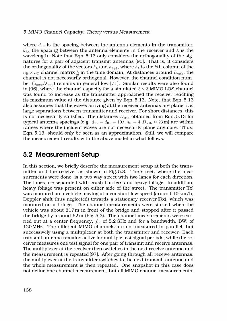
5 MIMO Channel Capacity: Theory versus Measurement
where dTx is the spacing between the antenna elements in the transmitter,dRx the spacing between the antenna elements in the receiver and λ is thewavelength. Note that Eqn. 5.13 only considers the orthogonality of the sig-natures for a pair of adjacent transmit antennas [95]. That is, it considersthe orthogonality of the vectors hk and hk+1, where hk is the kth column of thenR × nT channel matrix h in the time domain. At distances around Dorth, thechannel is not necessarily orthogonal. However, the channel condition num-ber (λmax/λmin) remains in general low [71]. Similar results were also foundin [96], where the channel capacity for a simulated 3 × 3 MIMO LOS channelwas found to increase as the transmitter approached the receiver reachingits maximum value at the distance given by Eqn. 5.13. Note, that Eqn. 5.13also assumes that the waves arriving at the receiver antennas are plane, i. e.large separations between transmitter and receiver. For short distances, thisis not necessarily satisfied. The distances Dorth obtained from Eqn. 5.13 fortypical antenna spacings (e.g. dTx = dRx = 10λ, nR = 4, Dorth ≈ 23 m) are withinranges where the incident waves are not necessarily plane anymore. Thus,Eqn. 5.13, should only be seen as an approximation. Still, we will comparethe measurement results with the above model in what follows.
5.2 Measurement Setup
In this section, we briefly describe the measurement setup at both the trans-mitter and the receiver as shown in Fig. 5.3. The street, where the mea-surements were done, is a two way street with two lanes for each direction.The lanes are separated with crash barriers and heavy foliage. In addition,heavy foliage was present on either side of the street. The transmitter (Tx)was mounted on a vehicle moving at a constant low speed (around 10 km/h,Doppler shift thus neglected) towards a stationary receiver (Rx), which wasmounted on a bridge. The channel measurements were started when thevehicle was about 217 m in front of the bridge and stopped after it passedthe bridge by around 62 m (Fig. 5.3). The channel measurements were car-ried out at a center frequency, fo, of 5.2 GHz and for a bandwidth, BW, of120 MHz. The different MIMO channels are not measured in parallel, butsuccessively using a multiplexer at both the transmitter and receiver. Eachtransmit antenna remains active for multiple test signal periods, while the re-ceiver measures one test signal for one pair of transmit and receive antennas.The multiplexer at the receiver then switches to the next receive antenna andthe measurement is repeated [97]. After going through all receive antennas,the multiplexer at the transmitter switches to the next transmit antenna andthe whole measurement is then repeated. One snapshot in this case doesnot define one channel measurement, but all MIMO channel measurements.
138
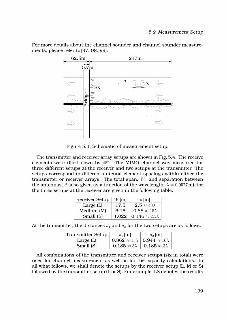
5.2 Measurement Setup
For more details about the channel sounder and channel sounder measure-ments, please refer to [97, 98, 99].
TxRx
Bri
dge
v
217m62.5m
5.7m
Figure 5.3: Schematic of measurement setup.
The transmitter and receiver array setups are shown in Fig. 5.4. The receiveelements were tilted down by 45o. The MIMO channel was measured forthree different setups at the receiver and two setups at the transmitter. Thesetups correspond to different antenna element spacings within either thetransmitter or receiver arrays. The total span, W , and separation betweenthe antennas, d (also given as a function of the wavelength, λ = 0.0577 m), forthe three setups at the receiver are given in the following table.
Receiver Setup W [m] d [m]
Large (L) 17.5 2.5 ≈ 43λMedium (M) 6.16 0.88 ≈ 15λ
Small (S) 1.022 0.146 ≈ 2.5λ
At the transmitter, the distances d1 and d2 for the two setups are as follows:
Transmitter Setup d1 [m] d2 [m]
Large (L) 0.862 ≈ 15λ 0.944 ≈ 16λSmall (S) 0.185 ≈ 3λ 0.185 ≈ 3λ
All combinations of the transmitter and receiver setups (six in total) wereused for channel measurement as well as for the capacity calculations. Inall what follows, we shall denote the setups by the receiver setup (L, M or S)followed by the transmitter setup (L or S). For example, LS denotes the results
139
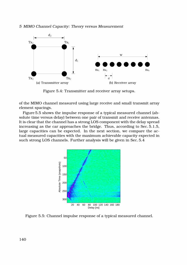
5 MIMO Channel Capacity: Theory versus Measurement
Tx1
Tx2Tx3
Tx4
d1
d2
(a) Transmitter array
Rx1 Rx8Rx2
d
W
(b) Receiver array
Figure 5.4: Transmitter and receiver array setups.
of the MIMO channel measured using large receive and small transmit arrayelement spacings.
Figure 5.5 shows the impulse response of a typical measured channel (ab-solute time versus delay) between one pair of transmit and receive antennas.It is clear that the channel has a strong LOS component with the delay spreadincreasing as the car approaches the bridge. Thus, according to Sec. 5.1.5,large capacities can be expected. In the next section, we compare the ac-tual measured capacities with the maximum achievable capacity expected insuch strong LOS channels. Further analysis will be given in Sec. 5.4
Delay [ns]
Abs
olut
e T
ime
(sna
psho
ts)
20 40 60 80 100 120 140 160 180
50
100
150
200
250
300
Figure 5.5: Channel impulse response of a typical measured channel.
140
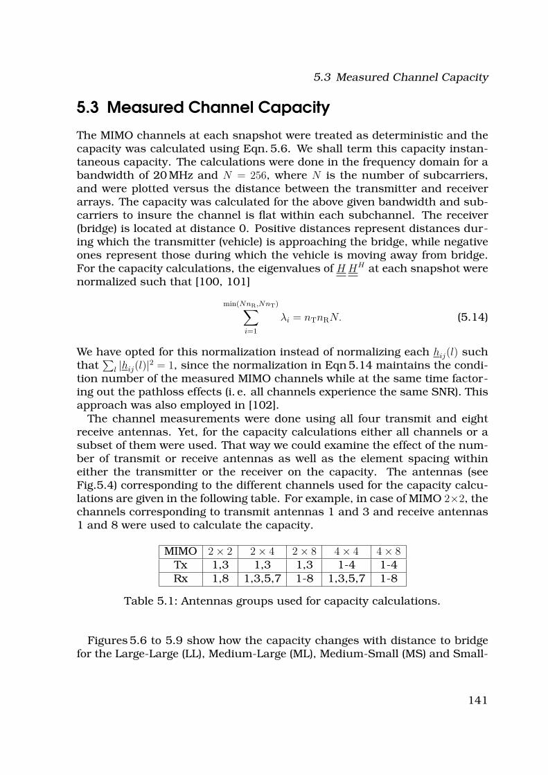
5.3 Measured Channel Capacity
5.3 Measured Channel Capacity
The MIMO channels at each snapshot were treated as deterministic and thecapacity was calculated using Eqn. 5.6. We shall term this capacity instan-taneous capacity. The calculations were done in the frequency domain for abandwidth of 20 MHz and N = 256, where N is the number of subcarriers,and were plotted versus the distance between the transmitter and receiverarrays. The capacity was calculated for the above given bandwidth and sub-carriers to insure the channel is flat within each subchannel. The receiver(bridge) is located at distance 0. Positive distances represent distances dur-ing which the transmitter (vehicle) is approaching the bridge, while negativeones represent those during which the vehicle is moving away from bridge.For the capacity calculations, the eigenvalues of H HH at each snapshot werenormalized such that [100, 101]
min(NnR,NnT)∑
i=1
λi = nTnRN. (5.14)
We have opted for this normalization instead of normalizing each hij(l) suchthat
∑
l |hij(l)|2 = 1, since the normalization in Eqn 5.14 maintains the condi-tion number of the measured MIMO channels while at the same time factor-ing out the pathloss effects (i. e. all channels experience the same SNR). Thisapproach was also employed in [102].
The channel measurements were done using all four transmit and eightreceive antennas. Yet, for the capacity calculations either all channels or asubset of them were used. That way we could examine the effect of the num-ber of transmit or receive antennas as well as the element spacing withineither the transmitter or the receiver on the capacity. The antennas (seeFig.5.4) corresponding to the different channels used for the capacity calcu-lations are given in the following table. For example, in case of MIMO 2×2, thechannels corresponding to transmit antennas 1 and 3 and receive antennas1 and 8 were used to calculate the capacity.
MIMO 2 × 2 2 × 4 2 × 8 4 × 4 4 × 8Tx 1,3 1,3 1,3 1-4 1-4
Rx 1,8 1,3,5,7 1-8 1,3,5,7 1-8
Table 5.1: Antennas groups used for capacity calculations.
Figures 5.6 to 5.9 show how the capacity changes with distance to bridgefor the Large-Large (LL), Medium-Large (ML), Medium-Small (MS) and Small-
141
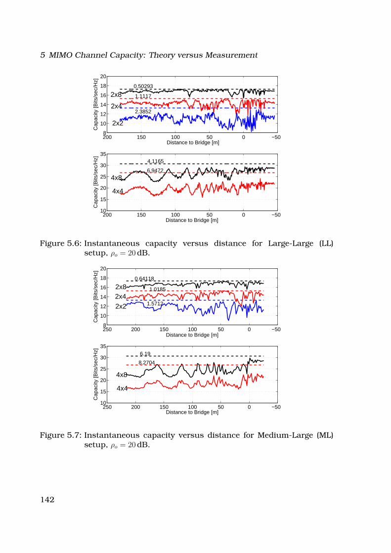
5 MIMO Channel Capacity: Theory versus Measurement
−500501001502008
10
12
14
16
18
20
2x2
2.3852
Distance to Bridge [m]
Cap
acity
[Bits
/sec
/Hz]
2x4
1.11172x80.50293
−5005010015020010
15
20
25
30
35
4x8
4.1165
Distance to Bridge [m]
Cap
acity
[Bits
/sec
/Hz]
4x4
6.9472
Figure 5.6: Instantaneous capacity versus distance for Large-Large (LL)setup, ρo = 20 dB.
−5005010015020025010
15
20
25
30
35
4x8
6.19
Distance to Bridge [m]
Cap
acity
[Bits
/sec
/Hz]
4x4
8.2704
−500501001502002508
10
12
14
16
18
20
2x2 1.5712
Distance to Bridge [m]
Cap
acity
[Bits
/sec
/Hz]
2x41.01852x8
0.64118
Figure 5.7: Instantaneous capacity versus distance for Medium-Large (ML)setup, ρo = 20 dB.
142
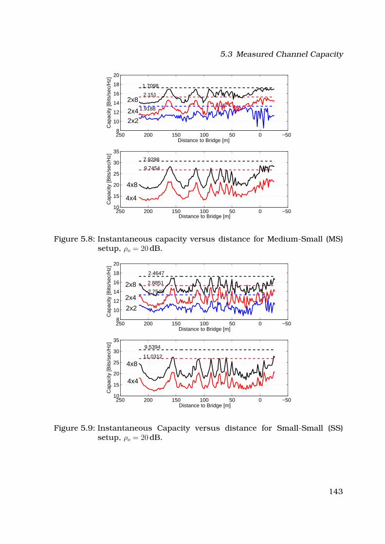
5.3 Measured Channel Capacity
−500501001502002508
10
12
14
16
18
20
2x2
1.9188
Distance to Bridge [m]
Cap
acity
[Bits
/sec
/Hz]
2x4
2.1512x8
1.7098
−5005010015020025010
15
20
25
30
35
4x8
7.9298
Distance to Bridge [m]
Cap
acity
[Bits
/sec
/Hz]
4x4
9.7454
Figure 5.8: Instantaneous capacity versus distance for Medium-Small (MS)setup, ρo = 20 dB.
−500501001502002508
10
12
14
16
18
20
2x2
2.7549
Distance to Bridge [m]
Cap
acity
[Bits
/sec
/Hz]
2x4
2.88512x8
2.4647
−5005010015020025010
15
20
25
30
35
4x8
9.5394
Distance to Bridge [m]
Cap
acity
[Bits
/sec
/Hz]
4x4
11.0312
Figure 5.9: Instantaneous Capacity versus distance for Small-Small (SS)setup, ρo = 20 dB.
143
5 MIMO Channel Capacity: Theory versus Measurement
Small (SS) array setups and different number of transmit and receive an-tennas for SNR=20 dB. The dashed horizontal lines represent the maximumcapacity that can be achieved for the given nR × nT MIMO system (Eqn. 5.12).The numbers on the lines are the difference between the mean capacity overdistance and the maximum one. As expected, the capacity increases as thenumber of either transmit or receive antennas is increased. Also, as thenumber of receive antennas increases, the gap between the measured ca-pacity and the maximum one decreases. In addition, the larger the antennaspacing, either at the transmitter or receiver, the higher the calculated ca-pacity.
Furthermore, the calculated capacities are seen to fluctuate as the trans-mitter approaches the receiver. This is especially true for small antennaspacing within either the transmitter or receiver arrays. Reflections from thestreet surface that lead to either destructive or constructive interference asthe vehicle moves may explain this behavior. To test this theory, the LOSmodel was extended to a two-path model. The results of the simulations willbe shown in Sec. 5.4. The figures also show that the fluctuations seem tobe more obvious the smaller the antenna element spacing within either thetransmitter or receiver arrays. Channel correlations, which are higher thecloser the antennas are to each other, are most probably the reason whythe fluctuations are more obvious in for example the SS setup than in theLL setup. In other words, the MIMO channels experience almost the samefading at all antennas the closer the antennas are to each other. This is es-pecially clear in the 2 × nR capacities, as we have chosen antennas that arefurthest from each other (see above table). In the LL setup, the 2 × nR MIMOchannel capacities experience no obvious fluctuations in contrast to the SSsetup. Antenna correlations will be discussed in more details in Sec. 5.5.
As mentioned in the previous section, the observed channels exhibit astrong LOS and we thus wish to compare the calculated capacities with themaximum achievable according to Sec. 5.1.5. The following table gives ap-proximate values for Dorth according to Eqn. 5.13. The same Dorth is obtainedfor nR = 4 and 8, since the distance between two receive antennas for nR = 4is twice that for nR = 8.
nR LL ML MS SS
2 600 m 213 m 40 m 7 m
4, 8 346 m 122 m 23 m 4 m
Table 5.2: Dorth for the different setups.
According to the above table, the LL setup as well as the ML with nR = 2 liewithin the orthogonal range through out the whole measurement distance.
144
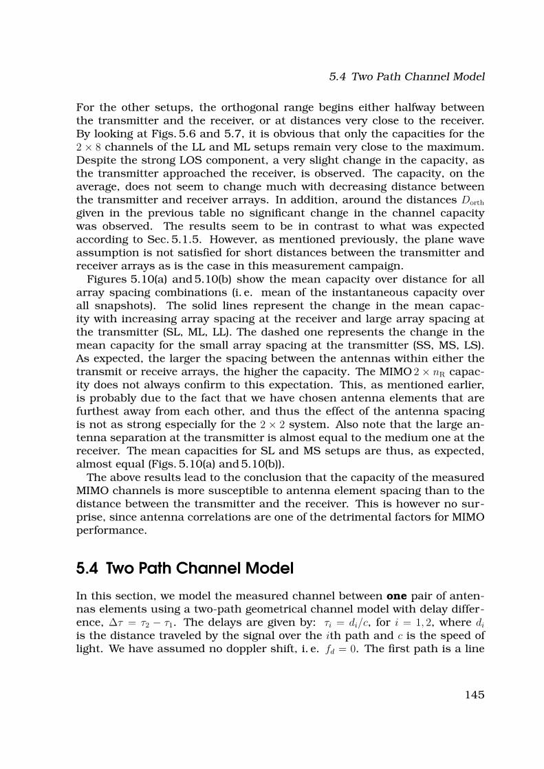
5.4 Two Path Channel Model
For the other setups, the orthogonal range begins either halfway betweenthe transmitter and the receiver, or at distances very close to the receiver.By looking at Figs. 5.6 and 5.7, it is obvious that only the capacities for the2 × 8 channels of the LL and ML setups remain very close to the maximum.Despite the strong LOS component, a very slight change in the capacity, asthe transmitter approached the receiver, is observed. The capacity, on theaverage, does not seem to change much with decreasing distance betweenthe transmitter and receiver arrays. In addition, around the distances Dorth
given in the previous table no significant change in the channel capacitywas observed. The results seem to be in contrast to what was expectedaccording to Sec. 5.1.5. However, as mentioned previously, the plane waveassumption is not satisfied for short distances between the transmitter andreceiver arrays as is the case in this measurement campaign.
Figures 5.10(a) and 5.10(b) show the mean capacity over distance for allarray spacing combinations (i. e. mean of the instantaneous capacity overall snapshots). The solid lines represent the change in the mean capac-ity with increasing array spacing at the receiver and large array spacing atthe transmitter (SL, ML, LL). The dashed one represents the change in themean capacity for the small array spacing at the transmitter (SS, MS, LS).As expected, the larger the spacing between the antennas within either thetransmit or receive arrays, the higher the capacity. The MIMO 2 × nR capac-ity does not always confirm to this expectation. This, as mentioned earlier,is probably due to the fact that we have chosen antenna elements that arefurthest away from each other, and thus the effect of the antenna spacingis not as strong especially for the 2 × 2 system. Also note that the large an-tenna separation at the transmitter is almost equal to the medium one at thereceiver. The mean capacities for SL and MS setups are thus, as expected,almost equal (Figs. 5.10(a) and 5.10(b)).
The above results lead to the conclusion that the capacity of the measuredMIMO channels is more susceptible to antenna element spacing than to thedistance between the transmitter and the receiver. This is however no sur-prise, since antenna correlations are one of the detrimental factors for MIMOperformance.
5.4 Two Path Channel Model
In this section, we model the measured channel between one pair of anten-nas elements using a two-path geometrical channel model with delay differ-ence, ∆τ = τ2 − τ1. The delays are given by: τi = di/c, for i = 1, 2, where di
is the distance traveled by the signal over the ith path and c is the speed oflight. We have assumed no doppler shift, i. e. fd = 0. The first path is a line
145
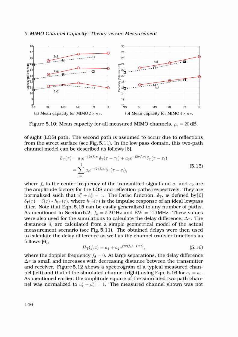
5 MIMO Channel Capacity: Theory versus Measurement
SS SL MS ML LS LL8
9
10
11
12
13
14
15
16
17
18
2x2
2x4
2x8
Cap
acity
[Bits
/sec
/Hz]
(a) Mean capacity for MIMO 2 × nR.
SS SL MS ML LS LL10
12
14
16
18
20
22
24
26
28
30
4x4
4x8
Cap
acity
[Bits
/sec
/Hz]
(b) Mean capacity for MIMO 4 × nR.
Figure 5.10: Mean capacity for all measured MIMO channels, ρo = 20 dB.
of sight (LOS) path. The second path is assumed to occur due to reflectionsfrom the street surface (see Fig. 5.11). In the low pass domain, this two-pathchannel model can be described as follows [6],
hT(τ) = a1e−j2πfoτ1δT(τ − τ1) + a2e
−j2πfoτ2δT(τ − τ2)
=2∑
i=1
aie−j2πfoτiδT(τ − τi),
(5.15)
where fo is the center frequency of the transmitted signal and a1 and a2 arethe amplitude factors for the LOS and reflection paths respectively. They arenormalized such that a2
1 + a22 = 1. The Dirac function, δT, is defined by [6]
δT(τ) = δ(τ) ∗ hLP(τ), where hLP(τ) is the impulse response of an ideal lowpassfilter. Note that Eqn. 5.15 can be easily generalized to any number of paths.As mentioned in Section 5.2, fo = 5.2 GHz and BW = 120 MHz. These valueswere also used for the simulations to calculate the delay difference, ∆τ . Thedistances di are calculated from a simple geometrical model of the actualmeasurement scenario (see Fig. 5.11). The obtained delays were then usedto calculate the delay difference as well as the channel transfer functions asfollows [6],
HT(f, t) = a1 + a2ej2π(fdt−f∆τ), (5.16)
where the doppler frequency fd = 0. At large separations, the delay difference∆τ is small and increases with decreasing distance between the transmitterand receiver. Figure 5.12 shows a spectrogram of a typical measured chan-nel (left) and that of the simulated channel (right) using Eqn. 5.16 for a1 = a2.As mentioned earlier, the amplitude square of the simulated two path chan-nel was normalized to a2
1 + a22 = 1. The measured channel shown was not
146
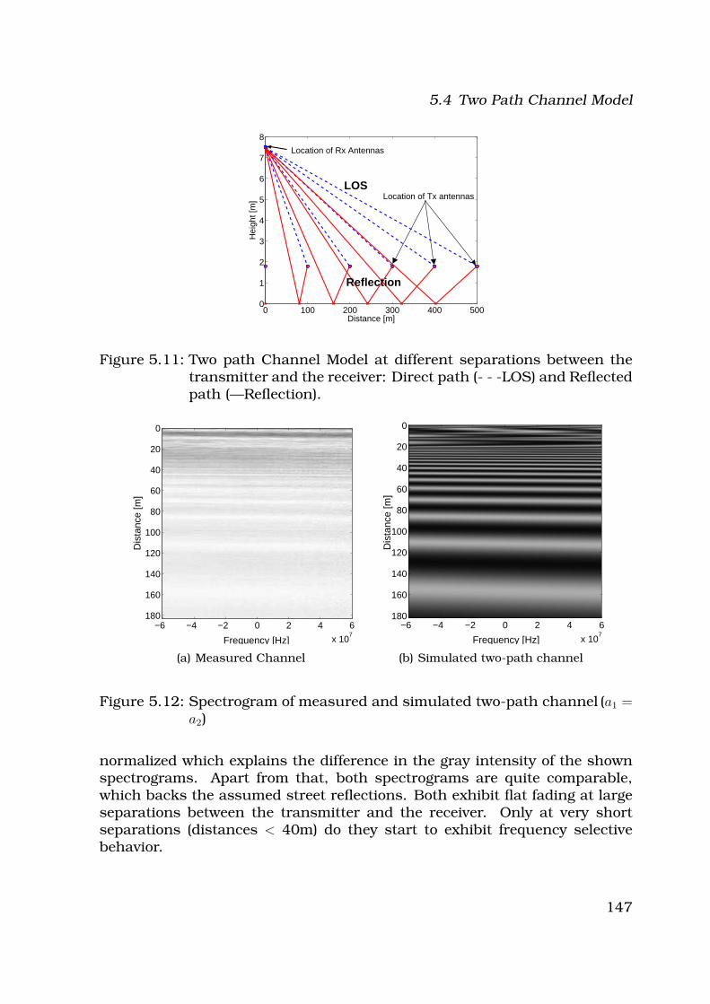
5.4 Two Path Channel Model
0 100 200 300 400 5000
1
2
3
4
5
6
7
8
Distance [m]
Hei
ght [
m]
LOS
Reflection
Location of Rx Antennas
Location of Tx antennas
Figure 5.11: Two path Channel Model at different separations between thetransmitter and the receiver: Direct path (- - -LOS) and Reflectedpath (—Reflection).
Dis
tanc
e [m
]
Frequency [Hz]
−6 −4 −2 0 2 4 6
x 107
0
20
40
60
80
100
120
140
160
180
(a) Measured Channel
Dis
tanc
e [m
]
Frequency [Hz]
−6 −4 −2 0 2 4 6
x 107
0
20
40
60
80
100
120
140
160
180
(b) Simulated two-path channel
Figure 5.12: Spectrogram of measured and simulated two-path channel (a1 =a2)
normalized which explains the difference in the gray intensity of the shownspectrograms. Apart from that, both spectrograms are quite comparable,which backs the assumed street reflections. Both exhibit flat fading at largeseparations between the transmitter and the receiver. Only at very shortseparations (distances < 40m) do they start to exhibit frequency selectivebehavior.
147
5 MIMO Channel Capacity: Theory versus Measurement
5.5 Antenna Correlations
To calculate the spatial correlation, ρij, between any pair of channel impulseresponses for antenna elements i and j, the following equation was applied[103, 104]
ρij =E{hih
∗j} − E{hi}E{h∗
j}√
(E{|hi|2} − |E{hi}|2)(E{|hj|2} − |E{hj}|2), (5.17)
where the denominator normalized the random variables. In Chapter 2,MIMO channel correlations were defined by the following equations,
kT
=1
nR
E{hHh}, (5.18)
kR
=1
nT
E{h hH}. (5.19)
The above equations basically correspond to Eqn. 5.17, where however inEqn. 5.18 the correlations are averaged over all receive antennas and inEqn. 5.19 they are averaged over all transmit antennas. They also assumethe channel to be zero mean and the average channel energy to be one. Thus,before the correlations can be calculated, the channel should be normalizedand the mean subtracted. In all what follows, the antenna correlations werecalculated using the second tap, the one with the highest amplitude. Thechannel mean was first calculated for 50 snapshots and subtracted, andthen the channel matrices were normalized. Finally, the correlations werecalculated by consecutively averaging over 200 snapshots.
Transmit Correlations
Figures 5.13 and 5.14 show the absolute values of the transmit correlationsfor the LL, SL, LS and SS setups respectively versus the snapshot num-ber. Larger snapshot values correspond to shorter distances between thetransmitter and receiver. The average of the correlations for antenna ele-ments lying behind each other for an observer on the bridge (Tx1 and Tx4as well as Tx2 and Tx3 in Figure 5.4(a)) are compared to the average of thecorrelations for all other antenna element combinations. In addition to thefact that the smaller the distance between the transmit antenna elementsthe higher the correlations, three important observations can be made fromthose figures. First, the antenna correlations are dependent of the geomet-rical setup of the antennas. Correlations for antennas lying behind eachother are in general higher than the correlations for all other antenna ele-ment combinations. This can be perceived best for the LL setup. Second,the transmit correlations are affected by the antenna configuration at the re-ceiver. By comparing the correlations for the LL and SL setups in Fig. 5.13,
148
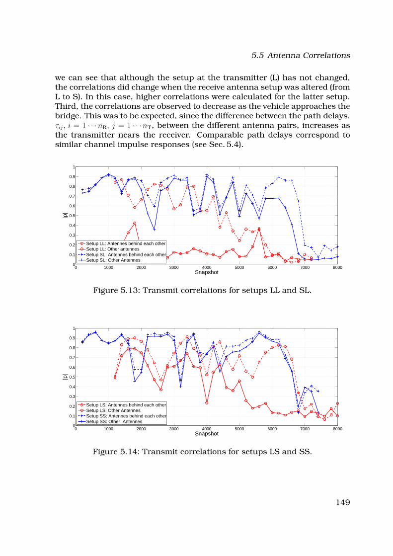
5.5 Antenna Correlations
we can see that although the setup at the transmitter (L) has not changed,the correlations did change when the receive antenna setup was altered (fromL to S). In this case, higher correlations were calculated for the latter setup.Third, the correlations are observed to decrease as the vehicle approaches thebridge. This was to be expected, since the difference between the path delays,τij, i = 1 · · ·nR, j = 1 · · ·nT, between the different antenna pairs, increases asthe transmitter nears the receiver. Comparable path delays correspond tosimilar channel impulse responses (see Sec. 5.4).
0 1000 2000 3000 4000 5000 6000 7000 80000
0.1
0.2
0.3
0.4
0.5
0.6
0.7
0.8
0.9
1
Snapshot
|ρ|
Setup LL: Antennes behind each otherSetup LL: Other antennesSetup SL: Antennes behind each otherSetup SL: Other Antennes
Figure 5.13: Transmit correlations for setups LL and SL.
0 1000 2000 3000 4000 5000 6000 7000 80000
0.1
0.2
0.3
0.4
0.5
0.6
0.7
0.8
0.9
1
Snapshot
|ρ|
Setup LS: Antennes behind each otherSetup LS: Other AntennesSetup SS: Antennes behind each otherSetup SS: Other Antennes
Figure 5.14: Transmit correlations for setups LS and SS.
149

5 MIMO Channel Capacity: Theory versus Measurement
1000 2000 3000 4000 5000 6000 7000 80000
0.1
0.2
0.3
0.4
0.5
0.6
0.7
0.8
0.9
1
Snapshot
|ρ|
Element spacing dElement spacing 2dElement spacing 3dElement spacing 4dElement spacing 5dElement spacing 6dElement spacing 7d
Figure 5.15: Receive correlations for ML Setup.
0 1000 2000 3000 4000 5000 6000 70000
0.1
0.2
0.3
0.4
0.5
0.6
0.7
0.8
0.9
1
Snapshot
|ρ|
Element spacing dElement spacing 2dElement spacing 3dElement spacing 4dElement spacing 5dElement spacing 6dElement spacing 7d
Figure 5.16: Receive correlations for MS Setup.
Receive Correlations
Figures 5.15 and 5.16 show the absolute value of the correlations betweenantenna elements at the receiver for the ML and MS setups. Shown are themeans of the correlations for antenna elements with same spacing, e. g. ρ4d
is the mean of ρ15, ρ26, ρ37 and ρ48. Similar to transmit correlations, the re-ceive correlations are affected by the transmit array configuration. Thus, theassumption of independence between the transmit and receive correlationsused in the Kronecker correlation model is not valid in this scenario. Similarobservations were also made in [105]. The receive correlations are also ob-served to decrease as the transmitter approaches the receiver. In addition,it can be seen from Figs. 5.15 and 5.16 and Table 5.3 that the correlations,in general, decrease as the element spacing increases. However, contraryto what is expected, the correlations for elements with spacing 7d are high
150
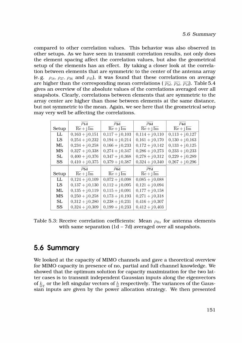
5.6 Summary
compared to other correlation values. This behavior was also observed inother setups. As we have seen in transmit correlation results, not only doesthe element spacing affect the correlation values, but also the geometricalsetup of the elements has an effect. By taking a closer look at the correla-tion between elements that are symmetric to the center of the antenna array(e. g. ρ18, ρ27, ρ36 and ρ45), it was found that these correlations on averageare higher than the corresponding mean correlations ( ρ5d, ρ3d, ρ1d). Table 5.4gives an overview of the absolute values of the correlations averaged over allsnapshots. Clearly, correlations between elements that are symmetric to thearray center are higher than those between elements at the same distance,but not symmetric to the mean. Again, we see here that the geometrical setupmay very well be affecting the correlations.
ρ1d ρ2d ρ3d ρ4d
Setup Re + j Im Re + j Im Re + j Im Re + j Im
LL 0,163 + j 0,151 0,117 + j 0,103 0,114 + j 0,110 0,113 + j 0,127LS 0,254 + j 0,232 0,194 + j 0,214 0,161 + j 0,170 0,130 + j 0,163ML 0,234 + j 0,258 0,166 + j 0,233 0,172 + j 0,142 0,133 + j 0,125MS 0,327 + j 0,338 0,274 + j 0,347 0,286 + j 0,273 0,233 + j 0,233SL 0,400 + j 0,376 0,347 + j 0,368 0,278 + j 0,312 0,229 + j 0,289SS 0,410 + j 0,375 0,379 + j 0,387 0,324 + j 0,340 0,267 + j 0,296
ρ5d ρ6d ρ7d
Setup Re + j Im Re + j Im Re + j Im
LL 0,124 + j 0,109 0,072 + j 0,098 0,085 + j 0,088LS 0,137 + j 0,130 0,112 + j 0,095 0,121 + j 0,094ML 0,135 + j 0,119 0,115 + j 0,091 0,177 + j 0,158MS 0,250 + j 0,258 0,173 + j 0,193 0,271 + j 0,318SL 0,312 + j 0,280 0,238 + j 0,231 0,416 + j 0,307SS 0,324 + j 0,309 0,199 + j 0,233 0,412 + j 0,403
Table 5.3: Receive correlation coefficients: Mean ρRx for antenna elementswith same separation (1d – 7d) averaged over all snapshots.
5.6 Summary
We looked at the capacity of MIMO channels and gave a theoretical overviewfor MIMO capacity in presence of no, partial and full channel knowledge. Weshowed that the optimum solution for capacity maximization for the two lat-ter cases is to transmit independent Gaussian inputs along the eigenvectorsof k
Tor the left singular vectors of h respectively. The variances of the Gaus-
sian inputs are given by the power allocation strategy. We then presented
151
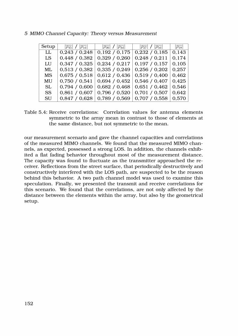
5 MIMO Channel Capacity: Theory versus Measurement
Setup |ρ45| / |ρ1d| |ρ36| / |ρ3d| |ρ27| / |ρ5d| |ρ18|LL 0,243 / 0,248 0,192 / 0,175 0,232 / 0,185 0,143LS 0,448 / 0,382 0,329 / 0,260 0,248 / 0,211 0,174LU 0,347 / 0,325 0,234 / 0,217 0,197 / 0,157 0,105ML 0,513 / 0,382 0,335 / 0,249 0,256 / 0,202 0,257MS 0,675 / 0,518 0,612 / 0,436 0,519 / 0,400 0,462MU 0,750 / 0,541 0,694 / 0,452 0,546 / 0,407 0,425SL 0,794 / 0,600 0,682 / 0,468 0,651 / 0,462 0,546SS 0,861 / 0,607 0,796 / 0,520 0,701 / 0,507 0,642SU 0,847 / 0,628 0,789 / 0,569 0,707 / 0,558 0,570
Table 5.4: Receive correlations: Correlation values for antenna elementssymmetric to the array mean in contrast to those of elements atthe same distance, but not symmetric to the mean.
our measurement scenario and gave the channel capacities and correlationsof the measured MIMO channels. We found that the measured MIMO chan-nels, as expected, possessed a strong LOS. In addition, the channels exhib-ited a flat fading behavior throughout most of the measurement distance.The capacity was found to fluctuate as the transmitter approached the re-ceiver. Reflections from the street surface, that periodically destructively andconstructively interfered with the LOS path, are suspected to be the reasonbehind this behavior. A two path channel model was used to examine thisspeculation. Finally, we presented the transmit and receive correlations forthis scenario. We found that the correlations, are not only affected by thedistance between the elements within the array, but also by the geometricalsetup.
152
Chapter6Summary and Conclusion
In recent years, there has been a continuous demand for reliable wirelesstransmission at even higher data rates. This trend is very unlikely tochange and, as a matter of fact, the demands are expected to increase.Thus, switching to MIMO communication systems is inevitable. In this work,several transmission techniques for MIMO-OFDM were studied. The aim wasto improve the system reliability depending on the amount of informationpresent at the transmitter and type of equalizer at the receiver mitigatingthe interference. We have focused our attention on two cases: no andpartial channel state information at the transmitter. Both are of practicalimportance, since full channel state information is hardly available at thetransmitter.
In Chapter 2, a detailed theoretical background for MIMO-OFDM as well asan overview of four block equalizers employed in this work for equalizationwas presented. Chapter 3 focused on the case of no channel state informa-tion at the transmitter. Two criteria, that need to be satisfied by spreadingmatrices if full diversity is to be achieved, were defined. A family of spreadingmatrices, MC-CAFS, which were devised based on those criteria was then
153
6 Summary and Conclusion
presented. In addition, we demonstrated how spreading and antenna corre-lations affect the interference and the matched filter bound and in turn theBER performance. The main conclusions of this chapter are as follows:
- Spreading improves the matched filter bound, but increases the inter-ference. The higher the diversity offered by the spreading matrix, thehigher the interference.
- Spreading with full diversity, although increases the interference to itsmaximum, leads to the lowest BER for a range of antenna correlations,0 to some ρ value. The width of this range depends on the equalizer usedas well as on the Eb/No. The range gets wider as the Eb/No increases.
- The matched filter bound is dependent not only on the diversity, butalso on the number of correlated diversity branches.
- Antenna correlations increase the interference, which makes it harderfor the equalizer to mitigate the interference as correlations increase. Inaddition, receive correlations worsen the matched filter bound.
- Rotated MC-CAFS can lead to lower BER. This is achieved at no extracost.
Chapter 4 concentrated on partial channel state information at the trans-mitter, yet an overview of precoding in presence of full channel state informa-tion at the transmitter was also presented. We considered precoding undercovariance information (transmit correlations knowledge). We showed thattransmitting in the direction of the transmit correlation eigenvectors at eachsubcarrier was the optimum direction for average pairwise error probabilityminimization. For the uncoded transmission, precoding was shown to im-prove the BER for all equalizers except for the MMSE-BLE. Coded transmis-sion with iterative equalization and decoding was also investigated in details.The results can be summarized as follows:
- At high Eb/No and for MIMO-OFDM and MC-CDM precoding leads tohigher BER since the matched filter bound worsens.
- Precoding along with MC-CAFS and SCE always achieved the lowestBER at high Eb/No.
- The BER is highly dependent on the interference in the channel and lesson the condition number. The RNN was shown to be especially sensitiveto interference and sometimes does not even converge.
- The code memory affects the BER performance. A code with low mem-ory improves the BER at low Eb/No compared to a high memory code.However, the reverse is true at high Eb/No.
154
- EXIT charts are a very useful convergence analysis tool that can aid indesigning the communication system, e. g. deciding on the code memoryand equalizer used.
Thus, with a powerful equalizer such as the SCE and a full diversity spread-ing matrix as MC-CAFS, precoding can significantly reduce the BER.
Finally, in Chapter 5 a theoretical overview for MIMO channel capacity wasgiven to demonstrate the potential of MIMO transmission. The capacity andthe antenna correlations for a measured outdoor scenario with a strong lineof sight were calculated and shown in this chapter. The measured capaci-ties were found to increase by increasing the number of transmit or receiveantennas, as well as by increasing the antenna element spacing within thetransmitter or receiver arrays which agrees with the theoretical predictions.Nonetheless, in contrast to the theories, we found that high antenna cor-relations are present even for large antenna element spacings. In addition,contrary to the theoretical Kronecker correlation model, the transmit corre-lations were found to depend on the receiver array configuration and viceversa.
155

6 Summary and Conclusion
156

AppendixAMatrix Basics
A.1 Matrix Basics
A.1.1 Inverse, Transpose and Hermitian
• (A B)−1 = B−1A−1
• (A B C · · · )−1 = · · ·C−1B−1A−1
• (AT )−1 = (A−1)T
• (A + B)T = AT + BT
• (A B)T = BT AT
• (A B C · · · )T = · · ·CT BT AT
• (AH)−1 = (A−1)H
• (A + B)H = AH + BH
157

A Matrix Basics
• (AB C · · · )H = · · ·CHBHAH
A.1.2 Trace, Determinant and Frobenious Norm
• Tr (A) =∑
i aii, where aii is the ith diagonal element of A
• Tr (A) =∑
i λi λi = eig(A)
• Tr (A) = Tr (AT )
• Tr (AB) = Tr (B A)
• Tr (A + B) = Tr (B + A)
• Tr (AB C) = Tr (B C A) = Tr (C AB)
• det (AB) = det (A) det (B)
• det (A−1) = 1/ det (A)
• det (A) = Πiλi λi = eig(A)
• ||A||2F =∑n
i=1
∑nj=1 |aij|2
• For an n × n positive definite matrix A
det (A) = Πiλi ≤ Πni=1aii.
Tr (A) =∑n
i=1 λi.
||A)||2F = Tr (AHA) =∑n
i=1 λ2i λi = eig(A) and λ2
i = eig(AHA)
158

A.2 Mathematical Definitions
A.2 Mathematical Definitions
A.2.1 Kronecker Product
Definition
A ⊗ B =
a11B · · · a1nB...
. . .
am1B · · · amnB
(A.1)
Properties of Kronecker product
• (A ⊗ B)T = AT ⊗ BT
• (A ⊗ B)−1 = A−1 ⊗ B−1
• (A ⊗ B)H = AH ⊗ BH
• (A ⊗ B) ⊗ C = A ⊗ (B ⊗ C)
• (A + B) ⊗ C = A ⊗ C + B ⊗ C
• A ⊗ (B + C) = A ⊗ B + A ⊗ C
• (A ⊗ B)(C ⊗ D) = (A ⊗ C)(B ⊗ D)
• rank(A ⊗ B) = rank(A) rank(B)
• For any m × m complex matrix A with eigenvalues λi, i = 1 · · ·m and ann × n complex matrix B with eigenvalues µj, j = 1 · · ·n, then
– the eigenvalues of A ⊗ B are λiµj, i = 1 · · ·m, j = 1 · · ·n– det(A ⊗ B) = det(A)rank(B) det(B)rank(A)
– Tr(A ⊗ B) = Tr(A) Tr(B)
A.2.2 Hadamard Product
Definition, for any two m × n matrices A and B
A ◦ B =
a11b11 · · · a1nb1n...
. . .
am1bm1 · · · amnbmn
(A.2)
159

A Matrix Basics
Properties of Hadamard product
• A ◦ B = B ◦ A
• A ◦ (B + C) = A ◦ B + A ◦ C
• A ◦ (λB) = λ(A ◦ B)
• Theorem For any two m × n matrices A and Brank(A ◦ B) ≤ rank(A) rank(B)
• Schur Product TheoremIf the square matrices A and B are positive semidefinite, then A ◦ B isalso positive semidefinite
• If the square matrices A and B are positive semidefinite, then
– det(A ◦ B) ≤ det(A) det(B)
– λmin(A ◦ B) ≥ λmin(A)λmin(B)
– λmax(A ◦ B) ≤ λmax(A)λmax(B)
160

AppendixBMathematical Notations, Symbolsand List of Abbreviations
Mathematical Notation
(·)∗ Conjugate(·)H Conjugate transpose of a matrix (·) (hermitian)det(·) Determinate of a matrix (·)BlkDiag([A · · ·Z]) Forms a block diagonal matrix from a set of matrices
diag(·) Diagonal of a matrix (·)Diag(·) Forms a diagonal matrix from a vectorE{x} Expected value a random variable x|| · ||2F Frobenious norm of a matrix (·)ℑ{·} Imaginary part of a complex number⊗ Kronecker productlog2 Log to the base of 2max(·) maximum of a set of elementsmin(·) minimum of a set of elementsrank(·) Rank of a matrix (·)
161

B Mathematical Notations, Symbols and List of Abbreviations
ℜ{·} Real part of a complex numberTr Trace of a matrix (·)(·)T Transpose of a matrix (·)var(x) Variance of a random variable xvec(·) Stacks the columns of a matrix (·) to form a vector
Symbols
α Matched filter bound measureB MC-CAFS: number of spreading frequencies per antennaβ Measure of interferenceβ1/2 Measure of interferenceCR Channel Capacityχ Condition numbereT
Eigenvalues of transmit correlation matrix
fd Doppler frequencyfg Cut-off frequency of low pass filterfo Center frequencyF
oFouier matrix
F Cholesky decompostion of channel correlation matrix
Φ(·) Correlation measure of a correlaion matrix (·)g(t) Receive signalh SISO channel vector in time domainh(l) MIMO channel matrix in time domain at lth tap
H Channel matrix in frequency domain
Heff
Effective Channel matrix in frequency domain
I(X,Y ) Mutual Information between random variables X and YI
NIdentiy matrix of size N × N
K Rician factork
TTransmit correlation matrix
kR
Receive correlation matrix
k Transmit or Receive correlation matrix
L Number of channel tapsLcp Length of cyclix prefixL(q) Log-likelihood Ratio of bit qλ Wavelengthλi ith eigenvalue of a matrixλmax Maximum eigenvalue of a matrix
162
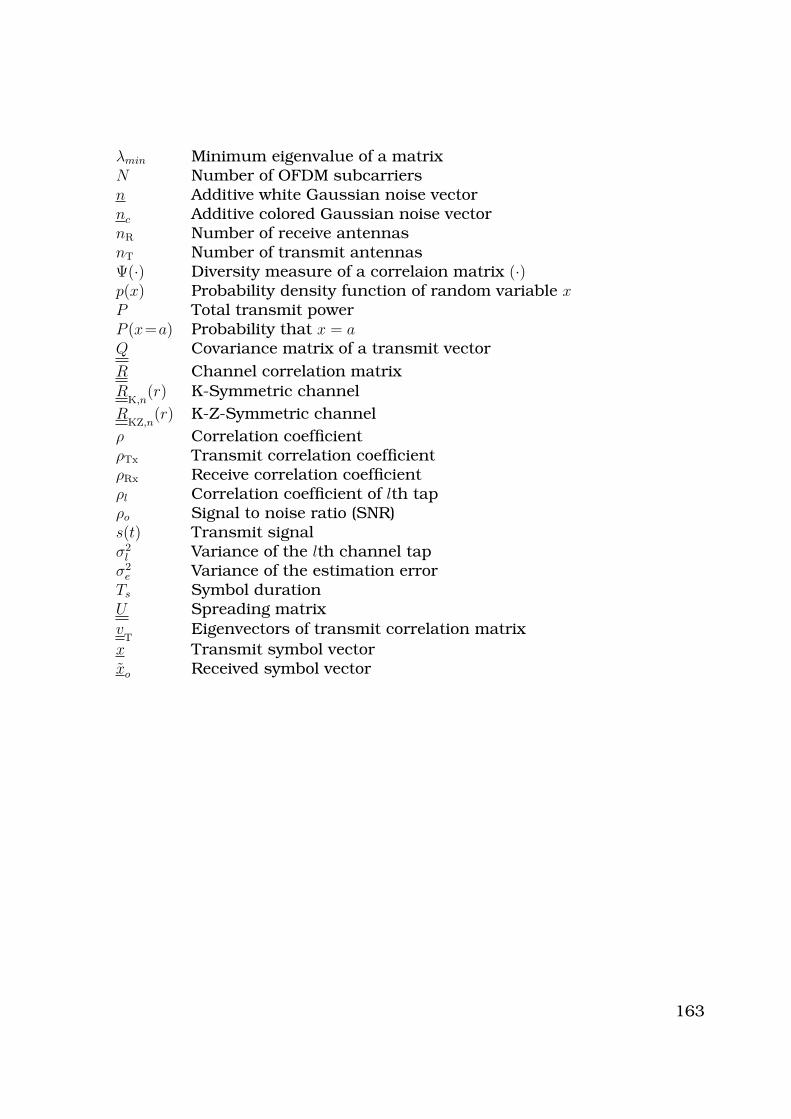
λmin Minimum eigenvalue of a matrixN Number of OFDM subcarriersn Additive white Gaussian noise vectornc Additive colored Gaussian noise vectornR Number of receive antennasnT Number of transmit antennasΨ(·) Diversity measure of a correlaion matrix (·)p(x) Probability density function of random variable xP Total transmit powerP (x=a) Probability that x = aQ Covariance matrix of a transmit vector
R Channel correlation matrix
RK,n
(r) K-Symmetric channel
RKZ,n
(r) K-Z-Symmetric channel
ρ Correlation coefficientρTx Transmit correlation coefficientρRx Receive correlation coefficientρl Correlation coefficient of lth tapρo Signal to noise ratio (SNR)s(t) Transmit signalσ2
l Variance of the lth channel tapσ2
e Variance of the estimation errorTs Symbol durationU Spreading matrix
vT
Eigenvectors of transmit correlation matrix
x Transmit symbol vectorxo Received symbol vector
163

B Mathematical Notations, Symbols and List of Abbreviations
List of Abbreviations
AWGN: Additive white Gaussion noiseBW BandwidthBWc Coherence BandwidthBER: Bit error rateCIR: Channel impulse responseCMF: Channel matched filterCP: Cyclic prefixCSI: Channel state informationCSIT: Channel state information at the transmitterDFT: Discrete Fourier transformEXIT: Extrinsic information transfer chartIBI: Inter block interferenceIDFT: Inverse discrete Fourier transformISCI: Inter subcarrier interferenceISI: Inter symbol interferenceLLR: Log-likelihood RatioLOS: Line of sightMC-CAFS: Multi-carrier cyclic antenna frequency spreadingMC-CDM: Multi-carrier code division multiplexingMFB: Matched filter boundMIMO: Multiple Input Multiple OutputMMSE-BDFE: Minimum mean square error block decision feedback equalizerMMSE-BLE: Minimum mean square error block linear equalizerMRC: Maximum Ratio CombiningOFDM: Orthogonal frequency division multiplexingpdf: Probability density functionPDP: Power delay profilePEP: Pairwise error probabilityPSK: Phase shift keyingRNN: Recurrent neural networksSCE: Soft Cholesky equalizerSISO: Single Input Single OutputSNR: Signal to noise ratioSTBC: Space Time Block Code
164

Bibliography
[1] I. Telatar, “Capacity of Multi-Antenna Gaussian Channels,” ATT Bell
Laboratoires, 1995.
[2] G. J. Foschini and M. J. Gans, “On limits of wirless communicationsin a fading environment when using multiple antennas,” Wireless Per-
sonal Communications, vol. 40, no. 6, pp. 311–335, Aug 1998.
[3] B. Holter, “On the capacity of the MIMO channel -a tutorialintroduction-,” http:// ilab0.ux.his.no/ norsig/ finalPapers/ 57.Capac-
ity of 1992001154555.pdf.
[4] I. Telatar, “Capacity of Multi-Antenna Gaussian Channels,” Euro Trans.
Telecommun., vol. 1, no. 6, pp. 585–595, Nov/Dec. 1999.
[5] O. Edfors, M. Sandell, J.-J. van de Beek, D. Landstrom, and F. Sjoberg,An introduction to orthogonal frequency division multiplexing. ResearchReport 1996/16, Lulea University of Technology, Sweden, 1996.
[6] J. Lindner, Informationsubertragung: Grundlagen der Kommunikation-
stechnik, 1st ed. Springer, 2004.
[7] A. Bury, Efficient Multi-Carrier Spread Spectrum Transmission. Disser-tation, Ulm University, VDI Verlag GmbH, 2001.
[8] J. Heiskala and J. Terry, OFDM Wireless LANs: A Theoretical and Prac-
tical Guide. Sams Publishing, 2002.
[9] A. Engelhart, Vector Detection Techniques with Moderate Complexity.Dissertation, Ulm University, VDI Verlag GmbH, 2003.
[10] K.-E. Kruger, Transformationen, 1st ed. Vieweg & Sohn, 2002.
165
Bibliography
[11] K.-D. Kammeyer and K. Kroschel, Digitale Signalverarbeitung: Filterung
und Spektralanalyse mit Matlab-Ubungnen, 5th ed. Teubner, 2002.
[12] J. Lindner, “Channel Coding and Modulation for Transmission overMultipath Channels,” Archiv fur Elekrtonik und Ubertragungstechnik,
AEU (International Jouranl of Electronics and Communications), vol. 49,no. 3, pp. 110–119, Jan. 1995.
[13] ——, “MC-CDMA and its Relation to General Mul-tiuser/MultisubchannelTransmission System,” IEEE Fourth Inter-
national Symposium on Spread Spectrum Techniques (IEEE ISSSTA’96),vol. 1, pp. 115–120, Sept. 1996.
[14] R. Zurmuhl and S. Falk, Matrizen und ihre Anwendungen, 4th ed.Springer-Verlag, 1984.
[15] J. Lindner, “MC-CDMA Spread Spectrum: An Attractive Special Case ofGeneral Multiuser/Multisubchannel Transmission Methods,” K. Fazel
and G.P. Fettweis (eds.), Multi-Carrier Spread-Sprectrum, Kluwer Aca-
demic Publishers, Netherlands, pp. 3–12, 1997.
[16] ——, “MC-CDMA in the Context of General Multiuser/MultisubchannelTransmission Methods,” European Trans. Telecomm., vol. 10, no. 5, pp.351–367, July/Aug. 1999.
[17] S. Hara and R. Prasad, Multicarrier Techniques for 4G Mobile Communi-
cations, 1st ed. Artech House, 2003.
[18] M. Dangl, D. Y. Yacoub, U. Marxmeier, W. G. Teich, and J. Lindner,“Performance of Joint Detection Techniques for Coded MIMO-OFDMand MIMO-MC-CDM,” in COST 273, Workshop on Broadband Wireless
Local Access, Paris/France, May 2003.
[19] D. Y. Yacoub, M. A. Dangl, U. Marxmeier, W. G. Teich, and J. Lindner,“Comparison of Iterative Detection Schemes for MIMO Systems withSpreading based on OFDM,” in 4th International Workshop on Multi-
Carrier Spread Spectrum (MC-SS), Oberpfaffenhofen/Germany, Sept.2003, pp. 101–111.
[20] J. G. Proakis, Digital Communications, 3rd ed. McGraw-Hill, 1998.
[21] E. Yoon, J. Hansen, and A. Paulraj, “Space-Frequency Precoding for anOFDM Based System Exploiting Spatial and Path Correlation,” in IEEE
GLOBECOM, vol. 1, 2004, pp. 436–440.
166
Bibliography
[22] A. Paulraj, R. Nabar, and D. Gore, Introduction to Space-Time Wireless
Communications, 1st ed. Cambridge Univ. Press, 2003.
[23] S. L. Loyka, “Channel Capacity of MIMO Architecture Using the Ex-ponential Correlation Matrix,” IEEE Comm. Letters, vol. 5, no. 9, pp.369–371, Sept. 2001.
[24] H. Shin, “MIMO Diversity in the Presence of Double Scattering,” insubmitted to IEEE transcations on Information Theory, vol. 1, 2005.
[25] R. A. Horn and C. R. Johnson, Topics in Matrix Analysis, 1st ed. Cam-bridge University Press, 1991.
[26] M. T. Ivrlac and J. A. Nossek, “Quantifying Diversity and Correlation inRayleigh Fading MIMO Communication Systems,” in IEEE International
Symposium on Signal Processing and Information Technology,ISSPIT’03,Darmstadt, Germany, Dec 2003.
[27] ——, “Diversity and Correlation in Rayleigh Fading MIMO Channels,” inIEEE Vehicular Technology Conference, VTC 2005, vol. 1, Spring 2005,pp. 151– 155.
[28] T. Betlehem, T. D. Abhayapala, and T. A. Lamahewa, “Space-TimeMIMO Channel Modelling using Angular Power Distributions,” in IEEE
7th Australian Communication Theory Workshop, vol. 1, 2006, pp. 163–168.
[29] G. K. Kaleh, “Channel Equalization for Block Transmission Systems,”IEEE Journal on Selected Areas in Communications, vol. 13, no. 1, pp.110–121, Jan. 1995.
[30] W. G. Teich and M. Seidl, “Code division multiple access communica-tions: Multiuser detection based on a recurrent neural network struc-ture,” in Proc. IEEE ISSSTA, vol. 3, Mainz/Germany, Sept. 1996, pp.979–984.
[31] J. Egle, C. Sgraja, and J. Lindner, “Iterative soft Cholesky block de-cision feedback equalizer – a promising approach to combat interfer-ence,” in Proc. IEEE VTC, vol. 3, Rhodes/Greece, May 2001, pp. 1604–1608.
[32] J. Egle and J. Lindner, “Iterative Joint Equalization and Decodingbased on Soft Cholesky Equalization for General Complex Valued Mod-ulation Symbols,” in DSPCS ’02 - 6th Int. Symposium on DSP for Com-
munication Systems, vol. 3, Sydney-Manly/Australia, 28-31 Jan. 2002,pp. 163–170.
167
Bibliography
[33] J. Egle, Detection Methods for Power and Bandwidth Efficient Single
Carrier Block Transmissions. Dissertation, Ulm University, VDI VerlagGmbH, 2004.
[34] M. A. Dangl, J. Egle, C. Sgraja, W. G. Teich, and J. Lindner, “Joint Iter-ative Equalization, Demapping, and Decoding with a Soft InterferenceCanceler,” in COST 289 meeting, Hamburg Germany, July 2003.
[35] ——, “Convergence of RNN Based Iterative Equalization and Decoding ,”in COST 262 MCM Meeting, TD 068(02), Prague/Czech Republic, Sept.2002.
[36] R. Bronson, Matrix Methods An Introduction, 2nd ed. Academic Press,1991.
[37] D. S. Watkins, Fundamentals of Matrix Computations, 1st ed. JohnWiley & Sons, 1991.
[38] C. Sgraja, A. Engelhart, W. G. Teich, and J. Lindner, “Equalization withrecurrent neural networks for complex-valued modulation schemes,”in Proc. 3rd Workshop Kommunikationstechnik, Reisensburg/Germany,June 1999.
[39] C. Sgraja, W. G. Teich, A. Engelhart, and J. Lindner, “Mul-tiuser/Multisubchannel Detection Based on Recurrent Neural Net-work Structures for Linear Modulation Schemes with general Complex-valued Symbol Alphabet,” in COST 262 Workshop Multiuser Detection in
Spread Spectrum Communications.
[40] A. Engelhart, W. G. Teich, J. Lindner, G. Jeney, S. Imre, and L. Pap,“A Survey of Multiuser/Multisubchannel Detection Schemes Basedon Recurrent Neural Networks,” Wireless Communications and Mobile
Computing, vol. 2, no. 3, pp. 269–284, May 2002.
[41] A. Engelhart, W. G. Teich, and J. Lindner, Complex Valued Signal Esti-
mation for Interference Cancellation Schemes. Technical Report, Uni-versity of Ulm, ITUU-TR-1998/4, 1998.
[42] T. Frey and M. Reinhardt, “Signal Estimation for Interference Cancel-lation and Cecision Feedback Equalization,” in IEEE Vehicular Technol-
ogy Conference, vol. 1, 1997, pp. 155–159.
[43] A. Papoulis and S. U. Pillai, Probability, Random Variables and Stochas-
tic Processes, 4th ed. Mc Graw Hill, 2002.
168
Bibliography
[44] C. Douillard, M. Jezequel, C. Berrou, A. Picart, P. Didier, andA. Glavieux, “Iterative correction of intersymbol interference: Turbo-equalization,” in European Trans. Telecomm., vol. 6, Sept/Oct. 1995,pp. 507–511.
[45] J. Hagenauer, E. Offer, and L. Papke, “Iterative Decoding of BinaryBlock and Convolutional Codes,” IEEE Transactions on Information The-
ory, vol. 42, no. 2, pp. 429–445, March 1996.
[46] B. Sklar, “A Primer on Turbo Code Concepts,” IEEE Communications
Magazine, pp. 94–101, Dec. 1997.
[47] C. Sgraja, A. Engelhart, W. G. Teich, and J. Lindner, “Combined equal-ization and decoding for BDFM packet transmission,” in 1st Interna-
tional OFDM-Workshop, Hamburg/Germany, Sept. 1999.
[48] M. A. Dangl, J. Egle, C. Sgraja, W. G. Teich, and J. Lindner, “Conver-gence Behavior of Iterative Equalization and Decoding Schemes withMemory,” in Proc. IEEE Global Telecommunications Conference (GLOBE-
COM), vol. 3, San Francisco (CA)/USA, Dec. 2003, pp. 1710–1715.
[49] ——, “Joint Iterative Equalization, Demapping, and Decoding with aSoft Interference Canceler,” in International Symposium on Communica-
tion Theory and Applications (ISCTA), Ambleside/England, July 2003,pp. 36–41.
[50] S. ten Brink, “Convergence of iterative decoding,” Electronic Letters,vol. 35, no. 10, pp. 806–808, May 1999.
[51] ——, “Designing Iterative Decoding Schemes with the Extrinsic Infor-mation Transfer Chart,” AEU International Journal of Electronics and
Communications, no. 6, pp. 389–398, Nov. 2000.
[52] ——, “Convergence Behavior of Iteratively Decoded Parallel Concate-nated Codes,” IEEE Transactions on Communications, vol. 49, no. 10,pp. 1727–1736, Oct. 2001.
[53] T. M. Cover and J. A. Thomas, Elements of Information Theory, 2nd ed.John Wiley & Sons, INC., 1991.
[54] J. Hagenauer, “The EXIT chart - Introduction to the Extrinsic Informa-tion Transfer in Iterative Processing,” in 12th European Signal Process-
ing Conference (EUSIPCO), Vienna/Austria, Sept. 2004, pp. 1541–1548.
169
Bibliography
[55] M. Moher, “An Iterative Multiuser Decoder for Near-Capacity Com-munications,” in IEEE Transactions on Communications, vol. 46, July1998, pp. 870–880.
[56] S. M. Alamouti, “A Simple Transmit Diversity Technique for WirelessCommunications,” IEEE Journal on Select areas in Communicaions,vol. 16, no. 8, pp. 1451–1457, Oct. 1998.
[57] V. Tarokh, N. Seshadri, and A. R. Calderbank, “Space-Time Codes forHigh Data Rate Wireless Communication: Performance Criterion andCode Construction,” IEEE Transactions on Information Theory, vol. 44,no. 2, pp. 744–763, March 1998.
[58] H. Boelsckei and A. J. Paulraj, “Space-Frequency Coded BroadbandOFDM Systems,” in IEEE WCNC, Sept. 2000.
[59] ——, “Space-Frequency Codes for Broadband Fading Channels,” in ISIT
2001, 2001.
[60] L. Shao, S. Roy, and S. Sandhu, “Rate-one Space Frequency Blockcodes with Maximum Diversity gain for MIMO-OFDM,” in IEEE Global
Telecommunications Conference - GLOBECOM 2003, Dec 2003, pp.809–813.
[61] D. Y. Yacoub, W. G. Teich, and J. Lindner, “MC-Cyclic Antenna Fre-quency Spread: A Novel Space-Frequency Spreading for MIMO-OFDM,”in COST 289 7th MCM: Spectrum and Power Efficient Broadband Com-
munications, Oberpfaffenhoffen/Germany, March 2005.
[62] ——, “MC-Cyclic Antenna Frequency Spread: A Novel Space-FrequencySpreading for MIMO-OFDM,” in 8th International Symposium on Com-
munication Theory and Applications (ISCTA ’05), Ambleside, Lake Dis-trict / UK, July 2005.
[63] R. Vaughan and J. B. Andersen, Channels, Propagation and Antennas
for Mobile Communications. The Institution of Engineering and Tech-nology, IET, 2003.
[64] D. Y. Yacoub, W. G. Teich, and J. Lindner, “MC-Cyclic Antenna Fre-quency Spread: Effect of Interference on the Performance of a SpreadMIMO-OFDM System,” in 10th International OFDM-Workshop, Ham-burg/ Germany, Aug./Sept. 2005, pp. 323–327.
[65] ——, “Effect of Antenna Correlations on Interference and Performanceof a Spread MIMO-OFDM System (MC-CAFS) ,” in 11th International
OFDM-Workshop, Hamburg/ Germany, Aug. 2006, pp. 111–115.
170
Bibliography
[66] J. Boutros and E. Viterbo, “Signal Space Diversity: A Power- andBandwidth-Efficient Diversity Technique for the Rayleigh Fading Chan-nel,” IEEE Trans. on Information Theory, vol. 44, no. 4, pp. 1453–1467,July 1998.
[67] Y. Xin, Z. Wang, and G. B. Giannakis, “Space-Time Diversity Systemsbased on Unitary Constellation-Rotating Precoders,” in IEEE Interna-
tional Conference on Acoustics, Speech and Signal Processing (ICASSP
2001), May 2001, pp. 2429–2432.
[68] Z. Liu, Y. Xin, and G. B. Giannakis, “Linear Constellation Precodingfor OFDM with Maximum Multipath Diversity and Coding gains,” IEEE
Transactions on Communications, vol. 51, no. 3, pp. 416–427, March2003.
[69] D. Y. Yacoub, W. G. Teich, and J. Lindner, “Rotated MC-Cyclic AntennaFrequency Spread: Effect of Rotations in Correlated MIMO-OFDM Sys-tems ,” in 7th IEEE International Workshop on Signal Processing Ad-
vances for Wireless Communications (SPAWC 2006), Cannes / France,July 2006.
[70] A. Bury, J. Egle, and J. Lindner, “Diversity Comparison of Spread-ing Transforms for Multicarrier Spread Spectrum Transmission,” IEEE
Transactions on Communications, vol. 51, no. 5, pp. 774–781, May2003.
[71] D. Y. Yacoub, E. Msechu, W. G. Teich, and J. Lindner, “Effect ofSpreading in an Outdoor MIMO-OFDM System,” in 9th International
OFDM-Workshop, Dresden/ Germany, Sept. 2004, pp. 12–16.
[72] M. Bossert, Channel Coding for Telecommunications. John Wiley &Sons Ltd, 1999.
[73] L. H. C. Lee, Convolutional Coding: Fundamentals and Applications.Artech House, 1997.
[74] D. Gerlach and A. Paulraj, “Adaptive Transmitting Antenna Methodsfor multipath Envornments,” in IEEE Globecom, 1994, pp. 425–429.
[75] D. Shiu and J. Kahn, “Power Allocation Strategies for Wireless Systemswith Multiple Transmit Antennas,” in Internal report of University of
California at Berekley, July 1998.
[76] M. Vu and A. Paulraj, “MIMO Wireless Linear Precoding,” accepted to
IEEE Signal Procccessing Magazine, 2006.
171
Bibliography
[77] D. P. Palomar, J. M. Cioffi, , and M. A. Lagunas, “Joint Tx-Rx Beam-forming Design for Multicarrier MIMO Channels: A Unified Frame-work for Convex Optimization,” IEEE Transactions on Signal Process-
ing, vol. 51, no. 9, pp. 2381–2401, Sept. 2003.
[78] H. Sampath, P. Stocia, and A. Paulraj, “Generalized Linear Precoderand Decoder Design for MIMO Channels using the Weighted MMSECritieron,” IEEE Transactions on Communications, vol. 49, no. 12, pp.2198–2206, Dec. 2001.
[79] G. G. Raleigh and J. M. Cioffi, “Spatio-temporal coding for wirelesscommunication,” IEEE Transactions on Communications, vol. 46, no. 3,pp. 357–366, March 1998.
[80] S. A. Jafar, S. Vishwanath, and A. Goldsmith, “Channel Capacity andBeamforming for Multiple Transmit and Receive Antennas with Covari-ance Feedback,” in Proc. ICC 2001, 2001.
[81] H. Sampath and A. Paulraj, “Linear Precoding for Space-Time CodedSystems with known Fading Correlations,” IEEE Communication Let-
ters, vol. 6, no. 6, pp. 239–241, June 2002.
[82] E. A. Jorswieck and H. Boche, “Channel Capacity and Capacity-Rangeof Beamforming in MIMO Wireless Systems under Correlated Fadingwith Covariance Feedback,” IEEE Transactions on Wireless Communi-
cations, vol. 3, no. 5, pp. 1543–1553, Sept 2004.
[83] S. A. Jafar and A. Goldsmith, “Transmitter Optimization and Optimal-ity of Beamforming for Multiple Antenna Systems,” IEEE Transactions
on Wireless Communications, vol. 3, no. 4, pp. 1165–1175, July 2004.
[84] Y. Zhao, R. Adve, and T. J. Lim, “Precoding of Orthogonal STBC withChannel Covariance Feedback for Minimum Error Probability,” in 15th
IEEE International Symposium on Personal, Indoor and Mobile Radio
Communications, PIMRIC 2004, vol. 1, Sept. 5-8 2004, pp. 503–507.
[85] M. Vu and A. Paulraj, “Optimal Linear Precoders for MIMO-WirelessCorrelated Channels With Nonzero Mean in Space-Time Coded Sys-tems,” IEEE Signal Transactions on Signal Processing, vol. 54, no. 6,pp. 2318–2332, June 2006.
[86] P. Xia, S. Zhou, and G. B. Giannakis, “Adaptive MIMO-OFDM BasedPartial Channel State Information,” IEEE Transactions on Signal Pro-
cessing, vol. 52, no. 1, pp. 202–213, Jan. 2004.
172
Bibliography
[87] S. Zhou and G. B. Giannakis, “Optimal Transmitter Eigen-Beamforming and Space-Time Block Coding Based on Channel MeanFeedback,” IEEE Transactions on Signal Processing, vol. 50, no. 10, pp.2599–2613, Oct. 2002.
[88] H. Boelsckei, M. Borgmann, and A. J. Paulraj, “Impact of the Propaga-tion Enviroment on the Perfomance of Space-Frequency Coded MIMO-OFDM,” IEEE Journal on selected areas in communications, vol. 21,no. 3, pp. 427–439, April 2003.
[89] S. Boyd and L. Vandenberghe, Convex Optimization. Cambridge Uni-versity Press, 2006.
[90] D. Y. Yacoub, W. G. Teich, and J. Lindner, “Precoding and Spreadingfor MIMO-OFDM in the Presence of Antenna Correlations ,” in 12th In-
ternational OFDM-Workshop, Hamburg/ Germany, Aug. 2007, pp. 105–109.
[91] G. Bauch, ,,Turbo-Entzerrung” und Sendeantennen-Diversity mit
,,Space-Time-Codes” im Mobilfunk. VDI-Verl., 2001, ISBN: 3-18-366010-5.
[92] G. J. Foschini, “Layered Space-Time Architecture for Wireless Com-munication in a Fading Enviorement when using Multi-Element An-tennas,” Bell Labs Technical Journal, pp. 41–59, Autumn 1996.
[93] S. A. Jafar and A. Goldsmith, “Beamforming Capacity and SNR Maxi-mization for Multiple Antenna Systems,” in VTC 2001, 2001, pp. 43–47.
[94] E. Visotsky and U. Madhow, “Space-Time Transmit Precoding with Im-perfect Feedback,” IEEE Transactions on Information Theory, vol. 4,no. 6, pp. 2632–2639, Sept 2001.
[95] D. Gesbert, H. Boelsckei, D. A. Gore, and A. Paulraj, “Outdoor MIMOWireless Channels: Models and Performance Prediction,” IEEE Trans-
action on Communications, vol. 50, no. 12, pp. 1926–1933, Dec. 2002.
[96] D. Y. Yacoub, W. G. Teich, and J. Lindner, “Capacity of Vehicle-BridgeMIMO Channels,” in COST 273, Workshop on Broadband Wireless Lo-
cal Access, 5th Management Committee Meeting, Lisbon/Portugal, Sept.2002.
[97] MEDAV GmbH, Uttenreuth: Channel Sounder, MIMO Extension,http://www.channelsounder.de/mimoconcept flash.htm.
173
Bibliography
[98] MEDAV GmbH, Uttenreuth: Broadband Vector Channel Sounder forMIMO Channels, www.channelsounder.de/medavdocs/RUSK-MIMO-Produktinfo-E W701WI.096 .pdf.
[99] R. S. Thoma, D. Hampicke, A. Richter, G. Sommerkorn, andU. Trautwein, “MIMO Vector Channel Sounder Measurement for SmartAntenna System Evaluation,” in European Transactions on Telecommu-
nications ETT, vol. 12, Sept. 2001, pp. 427–438.
[100] D. Y. Yacoub, W. G. Teich, and J. Lindner, “Capacity of Measured MIMOChannels in Dependence of Array Element Spacing and Distance be-tween Antennas ,” in International ITG - IEEE Workshop on Smart An-
tennas 2006, Reisensburg / Germany, March 2006.
[101] D. Y. Yacoub, C. Schneider, S. Warzuegel, W. G. Teich, R. Thom”a, andJ. Lindner, “Capacity of Measured MIMO Channels in Dependence ofArray Element Spacing and Distance between Antennas ,” in COST
289, Spectrum and Power Efficient Broadband Communications, 9th
MCM, Madrid / Spain, Nov 2005.
[102] F. Hagebolling, O. Weikert, and U. Zolzer, “Deterministic Predictionof Channel Capacity of Frequency Selective MIMO channels,” in 11th
International OFDM-Workshop, 2006, pp. 208–212.
[103] J. P. Kermoal, L. Schumacher, P. E. Mogensen, and K. I. Pedersenu,“Experimental Investigation of Correlation Properties of MIMO RadioChannels for Indoor Picocell Scenarios,” in IEEE Vehicular Technology
Conference, vol. 1, Fall 2000, pp. 14–21.
[104] P. Kyritsi, D. C. Cox, R. A. Valenzuela, and P. W. Wolniansky, “Correla-tion Analysis Based on MIMO Channel Measurements in an Indoor En-vironment,” IEEE Journal on Selected Areas in Communications, vol. 21,no. 5, pp. 713–720, June 2003.
[105] C. Zimmerman, M. Paasch, O. Weikert, and U. Zolzer, “On InvestigatingSpatial Correlations of MIMO Indoor Channels,” in 12th International
OFDM-Workshop, 2007, pp. 276–280.
[106] D. Y. Yacoub, B. Baumgartner, W. G. Teich, and J. Lindner, “Precod-ing and spreading for coded MIMO-OFDM,” in International ITG - IEEE
Workshop on Smart Antennas WSA, Darmstadt / Germany, Feb. 2008,pp. 296–303.
174
Index
AAlamouti Space Time Block
code . . . . . . . . . . . . . . . . . . . . . . 44
Antenna Correlations . 16, 96, 148
Capacity . . . . . . . . . . . . . . . . . . . 136
Frequency Domain . . . . 96, 120
Kronecker Model . . . . . . . . . . . . 17
Measurement Results . . . . . 148
BBlock Decision Feedback Equal-
izer . . . . . . . . . . . . . . . . . . . . . . . 24
MMSE-BDFE .. . . . . . . . . . . . . . . 24
ZF-BDFE .. . . . . . . . . . . . . . . . . . . 24
Block Equalizers . . . . . . . . . . . . . . . . 22
Block Decision FeedbackEqualizer . . . . . . . . . . . . . . . . 24
Block Linear Equalizer . . . . . 23
Recurrent Neural NetworkEqualizer (RNN) . . . . . . . . . 25
Soft Cholesky Equalizer(SCE) . . . . . . . . . . . . . . . . . . . . . 27
Block Linear Equalizer . . . . . . . . . 23
MMSE-BLE .. . . . . . . . . . . . . . . . . 23
ZF-BLE .. . . . . . . . . . . . . . . . . . . . . 23
CCapacity . . . . . . . . . . . . . . . . . . . . . . . 131
Antenna Correlations . . . . . 136
Line of Sight . . . . . . . . . . . . . . . 136
Cholesky Decomposition . . . . . . . 24
Coherence Bandwidth . . . . . . . . . . 55Condition Number . . . . . . . . . . . . . . 19Correlation Measure . . . . . . . . . . . . 20
DDiscrete Fourier Transform .. . . . 8Diversity . . . . . . . . . . . . . . . . . . . . . . . . . 42Diversity Measure . . . . . . . . . . . . . . 19
EEXIT Chart . . . . . . . . . . . . . . . . . . . . . . 32
Transient Trajectory . . . . . . . . 34Exponential Correlation Model 18
HHard Decision Equalizers . . . . . . 23
IIterative Equalization and Decod-
ing . . . . . . . . . . . . . . . . . . . . . . . 29Feedback Equalizers . . . . . . . . 31
KK-Symmetric Channel . . . . . . . . . . 34K-Z-Symmetric Channel . . . . . . . 35Kronecker Correlation Model . . 17,
59, 85
LLog-Likelihood Ratios (L-values) 30
MMatched Filter Bound . . . . . . 40, 60
175
Index
Matrix Vector Transmission ModelMIMO-OFDM .. . . . . . . . . . . . . . . 13Precoding . . . . . . . . . . . . . . . . . . . . 91SISO-OFDM .. . . . . . . . . . . . . . . . 10Spreading . . . . . . . . . . . . . . . . . . . 14
MC-CAFS .. . . . . . . . . . . . . . . . . . . . . . 49MC-CDM .. . . . . . . . . . . . . . . . . . . . . . . 48Measure of Interference . . . . 59, 60Measure of matched filter
bound . . . . . . . . . . . . . . . . . . . . 60MIMO .. . . . . . . . . . . . . . . . . . . . . . . . . . . . 4
Channel capacity . . . . . . . . . . 131Channel model . . . . . . . . . . . . . . . 4
MIMO-OFDM .. . . . . . . . . . . . . . . . . . 13Antenna correlations . . . . . . . 16Precoding . . . . . . . . . . . . . . . 93, 96Spreading Criteria . . . . . . . . . . 46
Mutual Information . . . . . . . . . . . . 32
OOFDM .. . . . . . . . . . . . . . . . . . . . . . . . . . . . 5
Cyclic prefix . . . . . . . . . . . . . . . . . . 7MIMO-OFDM .. . . . . . . . . . . . . . . 11
Antenna correlations . . . . . 16Channel model . . . . . . . . . . . . 12
SISO-OFDM .. . . . . . . . . . . . . . . . . 5Spreading . . . . . . . . . . . . . . . . . . . 14
PPairwise Error Probability . . . . . . 45Precoding . . . . . . . . . . . . . . . . . . . . . . . 91
Full channel knowledge . . . . 93Power Allocation Strate-
gies . . . . . . . . . . . . . . . . . . . . . . . 94Partial channel knowledge . 94
Flat Fading Channels . . . . . 95Frequency Selective Chan-
nels . . . . . . . . . . . . . . . . . . . . . . 96
RRecurrent Neural Network Equal-
izer (RNN) . . . . . . . . . . . . . . . . 25Rotated MC-CAFS .. . . . . . . . . . . . . 72
SSoft Cholesky Equalizer (SCE) . 27Soft Decision Equalizers . . . . . . . 25Space Frequency codes . . . . . . . . 46Space Time codes . . . . . . . . . . . . . . . 44
Alamouti . . . . . . . . . . . . . . . . . . . . . 44Spreading Matrices
MC-CAFS .. . . . . . . . . . . . . . . . . . . 49MC-CDM .. . . . . . . . . . . . . . . . . . . 48Rotated MC-CAFS .. . . . . . . . . 72
TTest Channels . . . . . . . . . . . . . . . . . . 34
K-Symmetric Channel . . . . . . 34K-Z-Symmetric Channel . . . . 35
Transient Trajectory . . . . . . . . . . . . 34
176

![Reduction PAPR of OFDM Signals by Combining Grouped ...Z. P. Wang, S. F. Chen 138 4. Grouped DCT Precoding The paper, by Park al.,et [10] proposes a scheme for PAPR reduction in OFDM](https://img.pdfslide.net/doc/110x75/604deb8294aed630874d7f6d/reduction-papr-of-ofdm-signals-by-combining-grouped-z-p-wang-s-f-chen-138.jpg)
![Circularly Pulse-Shaped Precoding for OFDM: A New Waveform ... · literature (e.g., [32]–[34]) often have undesirable complexity and compatibility issues for 5G NR actualization](https://img.pdfslide.net/doc/110x75/5ecbebcd667b0365126a35a9/circularly-pulse-shaped-precoding-for-ofdm-a-new-waveform-literature-eg.jpg)


![Improved N-continuous OFDM for 5G Wireless Communications · to-noise ratio (SNR) loss with high complexity. In the precoding methods [10–12], complicate decoding In the precoding](https://img.pdfslide.net/doc/110x75/5d54994988c993134b8b7e64/improved-n-continuous-ofdm-for-5g-wireless-communications-to-noise-ratio-snr.jpg)