Embed Size (px)
Citation preview
C. L. Cox Relaxation Processes in Glass
and Polymers, Lecture 4
Special Topics in Relaxation in Glass and Polymers
Lecture 4: Differential Equations
Dr. Chris Cox
Department of Mathematical Sciences
Clemson University
C. L. Cox Relaxation Processes in Glass
and Polymers, Lecture 4 Outline • Fourier transform solution of differential equations
• Brief review
• Ordinary differential equation
• Partial differential equation (heat equation)
• Laplace transform solution of differential equations
• Brief review
• Spring-mass equation
• System of equations
• Quiz (multiple-choice)
Resources • Erwin Kreysig, Advanced Engineering Mathematics, 5th edition.
• Chapters 5 (Laplace Transformation) & 12: Complex Numbers. Complex Analytic Functions • Gilbert Strang, Introduction to Applied Mathematics
• Section 4.3: Fourier Integrals • George W. Scherer, Relaxation in Glass and Composite, 1992
• Appendix A: Laplace Transform • Stanley J. Farlow, Partial Differential Equations for Scientists and Engineers, Dover, 1993
• Lesson 12: The Fourier Transform and Its Application to PDEs
C. L. Cox Relaxation Processes in Glass
and Polymers, Lecture 4 Fourier Transform Method Some more historical background
In 1811, Fourier submitted to the French Academy of Sciences a revised version of the rejected 1807 paper. The new version won a prize but was still refused publication because some details were deemed unclear by the reviewers.
The Fourier transform actually appeared in writings of Cauchy and Laplace, starting around 1782.
Most of the 1822 results plus new results were finally published by Fourier in 1822.
-Peter V. O’Neil, Advanced Engineering Mathematics
Lithograph of Joseph Fourier, 1768-1830, by Jules Boilly, 1823, in the Academy of Sciences, Paris.
C. L. Cox Relaxation Processes in Glass
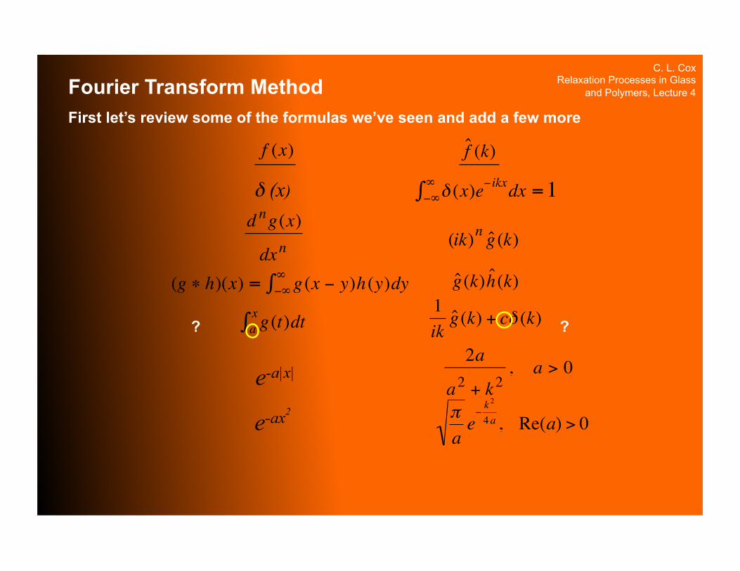
and Polymers, Lecture 4 Fourier Transform Method First let’s review some of the formulas we’ve seen and add a few more
? ?
€
ˆ f (k)
€
f (x)
€
d ng(x)
dxn
€
(ik)n ˆ g (k)
€
2a
a2 + k2, a > 0e-a|x| €
(g ∗ h)(x) = g (x − y)h (y)dy−∞∞∫
€
ˆ g (k) ˆ h (k)
e-ax2
€
πae−k 2
4a , Re(a) > 0€
g (t)dtax∫
€
1ik
ˆ g (k) + cδ (k)€
δ (x)e−ikxdx−∞∞∫ =1δ (x)
C. L. Cox Relaxation Processes in Glass
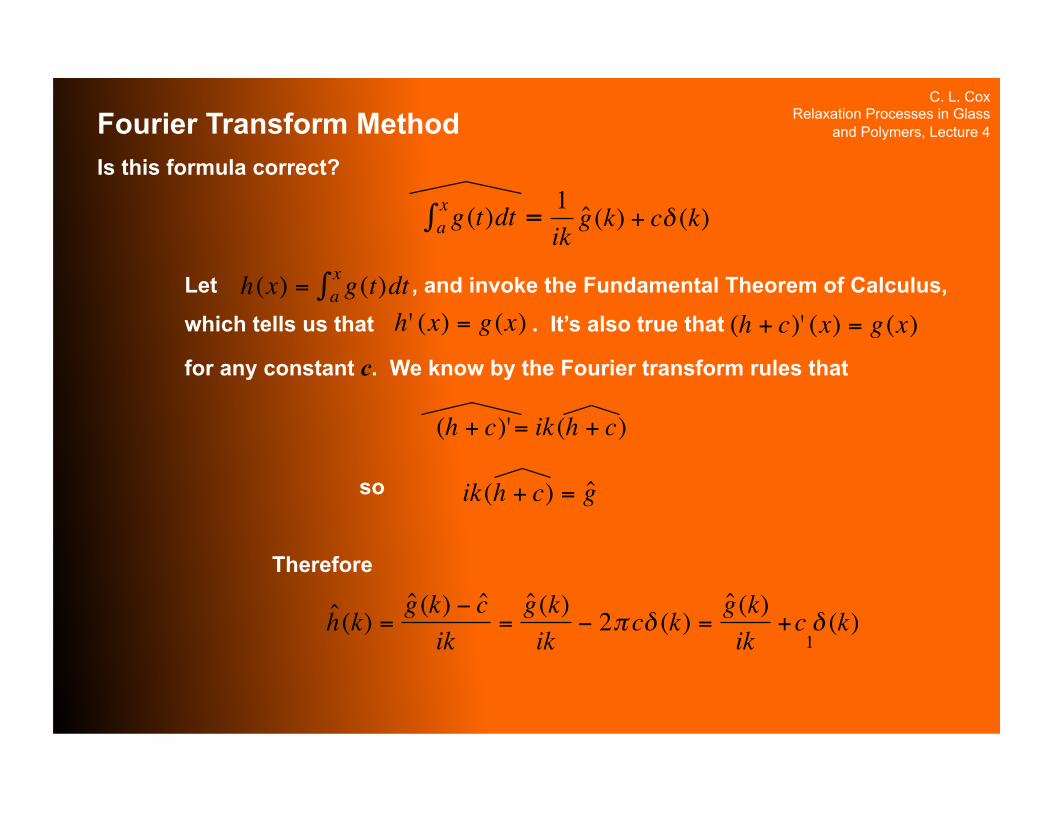
and Polymers, Lecture 4 Fourier Transform Method Is this formula correct?
Let , and invoke the Fundamental Theorem of Calculus,
which tells us that . It’s also true that
for any constant c. We know by the Fourier transform rules that
so
Therefore
€
g (t)dtax∫ =
€
1ik
ˆ g (k) + cδ (k)
€
h(x) = g(t)dtax∫
€
h' (x) = g (x)
€
(h + c)' (x) = g (x)
€
(h + c)'= ik (h + c)
€
ik(h + c) = ˆ g
€
ˆ h (k) =ˆ g (k) − ˆ c
ik=
ˆ g (k)ik
− 2π cδ (k) =ˆ g (k)ik
+c1δ (k)

C. L. Cox Relaxation Processes in Glass
and Polymers, Lecture 4 Fourier Transform Method for Solving Differential Equations
• Primarily used for linear differential equations with constant coefficients
• General step in applying method:
• Choose the appropriate form of the transform* • Apply FT to the differential equation
• Solve the resulting equation in the transform domain
• Invert the transform solution to find the solution of the original problem
* Depending on the range of independent variable, other forms of the Fourier transform may be desirable. For partial differential equations, the form of the boundary conditions may influence the decision.
For example, if the domain is 0 < x < , then a Fourier Cosine or Sine Transform may be better for the problem. These are defined as
and
(we‘ll focus on problems making use of the FT as we originally defined it) €
∞
€
ˆ f c
(k) = f (x) cos(kx)dx0∞∫
€
ˆ f s(k) = f (x) sin(kx)dx0
∞∫

C. L. Cox Relaxation Processes in Glass
and Polymers, Lecture 4 Fourier Transform Method Example 1: An ordinary differential equation
Consider the differential equation
Take the Fourier transform term by term, using linearity and the derivative rule:
Solve for :
Take the inverse transform to find :
Could we write the solution in terms of rather than ?
€
−d2udx 2
+ a2u = h(x), −∞ < x <∞
€
−(ik)2 ˆ u (k) + a2 ˆ u (k) = ˆ h (k)
€
ˆ u (k)
€
ˆ u (k) =ˆ h (k)
a2 + k 2
€
u(x)
€
u(x) =1
2π
ˆ h (k)
a2 + k 2 eikxdk−∞∞∫
€
h(k)
€
ˆ h (k)
C. L. Cox Relaxation Processes in Glass
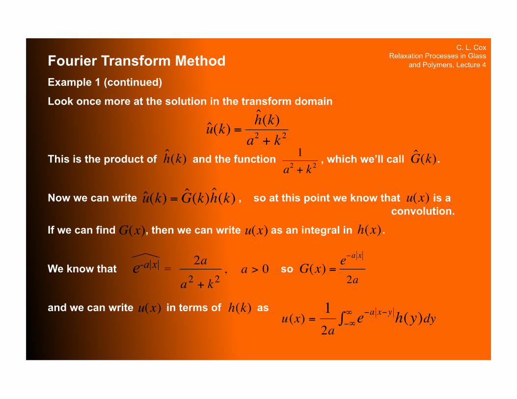
and Polymers, Lecture 4 Fourier Transform Method Example 1 (continued)
Look once more at the solution in the transform domain
This is the product of and the function , which we’ll call .
Now we can write , so at this point we know that is a convolution.
If we can find , then we can write as an integral in .
We know that so
and we can write in terms of as
€
ˆ u (k) =ˆ h (k)
a2 + k 2
€
ˆ h (k)
€
1a2 + k 2
€
ˆ G (k)
€
ˆ u (k) = ˆ G (k) ˆ h (k)
€
u(x)
€
G(x)
€
u(x)
€
h(x)
€
2a
a2 + k2, a > 0e-a|x| =
€
G(x) =e−a x
2a
€
u(x)
€
h(k)
€
u(x) =12a
e−a x−y h(y)dy−∞∞∫

C. L. Cox Relaxation Processes in Glass
and Polymers, Lecture 4 Fourier Transform Method Example 2: A partial differential equation – the heat equation
Heat flow in an infinite rod with initial temperature is governed by the initial value problem
Taking the Fourier transform term by term with respect to x will turn the partial differential equation into a first order ordinary equation.
Applying FT to the pde and the initial condition:
Keep in mind that actually depends on k and t , but we can treat the problem in the transform domain as an ode.
€
∂u∂t
= c 2 ∂2u∂x 2
, −∞ < x <∞, 0 < t <∞
€
φ(x)
€
u(x,0) = φ(x), −∞ < x <∞
€
d ˆ u dt
= −c 2k 2 ˆ u
€
ˆ u (k,0) = ˆ φ (k)
€
ˆ u
C. L. Cox Relaxation Processes in Glass
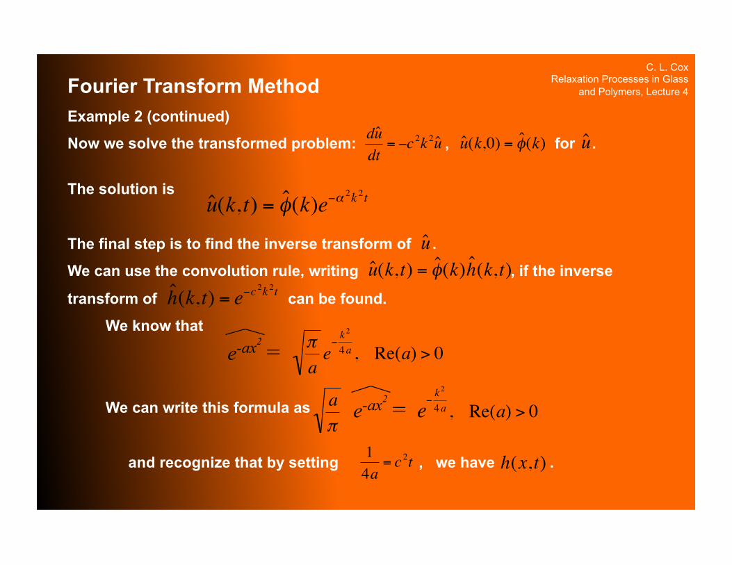
and Polymers, Lecture 4 Fourier Transform Method Example 2 (continued)
Now we solve the transformed problem: , for .
The solution is
The final step is to find the inverse transform of .
We can use the convolution rule, writing , if the inverse
transform of can be found.
We know that
We can write this formula as
and recognize that by setting , we have .
€
d ˆ u dt
= −c 2k 2 ˆ u
€
ˆ u (k,0) = ˆ φ (k)
€
ˆ u
€
ˆ u (k, t) = ˆ φ (k)e−α2k 2t
€
ˆ u
€
ˆ u (k, t) = ˆ φ (k) ˆ h (k, t)
€
ˆ h (k, t) = e−c 2k 2t
e-ax2 =
€
πae−k 2
4a , Re(a) > 0
€
aπ
e−k 2
4a , Re(a) > 0e-ax2 =
€
14a
= c 2t
€
h(x, t)

C. L. Cox Relaxation Processes in Glass
and Polymers, Lecture 4 Fourier Transform Method Example 2 (continued)
Summarizing what we just found:
We know that the Fourier transform of the solution of our initial value problem has the form
with
as long as we set , i.e.
Therefore,
and finally,
Comment: What we refer to as is often called , for Green’s function,
and it has interesting interpretations from both physical and mathematical perspectives.
€
ˆ u (k, t) = ˆ φ (k) ˆ h (k, t)
€
ˆ h (k, t) = e−c 2k 2t =aπ
πa
e−c 2k 2t =
€
14a
= c 2t
€
a =14c 2t
€
aπ
€
e−ax2
€
h(x, t) =aπe−ax
2
=1
4πc 2te−x 2
4c 2t =1
2c π te−x 2
4 c 2t
€
u(x, t) = φ(x)∗ h(x,t) = φ(x − y)−∞∞∫
12c π t
e−y 2
4 c 2t dy
€
h(x, t)
€
G(x, t)
C. L. Cox Relaxation Processes in Glass
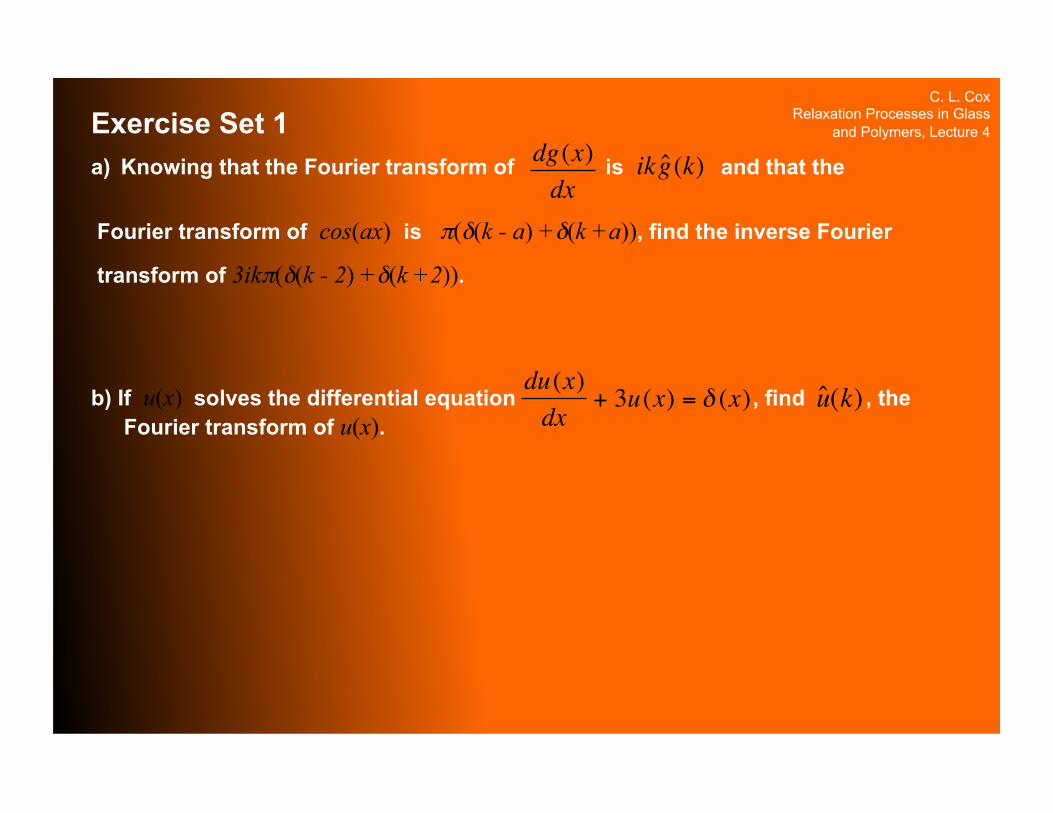
and Polymers, Lecture 4 Exercise Set 1 a) Knowing that the Fourier transform of is and that the
Fourier transform of cos(ax) is π(δ(k - a) +δ(k +a)), find the inverse Fourier
transform of 3ikπ(δ(k - 2) +δ(k +2)).
b) If u(x) solves the differential equation , find , the Fourier transform of u(x).
€
dg(x)dx
€
ik ˆ g (k)
€
du(x)dx
+ 3u(x) = δ (x)
€
ˆ u (k)

C. L. Cox Relaxation Processes in Glass
and Polymers, Lecture 4 Laplace Transform Method Some more historical background
The transform actually originates with Leonhard Euler (1707-1783), the Swiss mathematician. The Italian-French mathematical physicist Joseph Louis Lagrange (1736-1813) used similar integrals for work in probability theory. This work influenced Laplace.
- Paul J. Nahin, Behind the Laplace transform, IEEE Spectrum, March 1991.
Pierre-Simon Laplace (1749–1827). Posthumous portrait by Madame Feytaud, 1842.
C. L. Cox Relaxation Processes in Glass
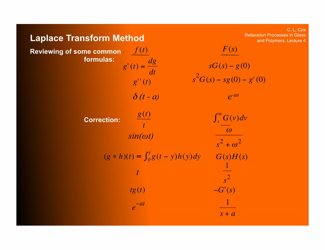
and Polymers, Lecture 4 Laplace Transform Method Reviewing of some common
formulas:
Correction:
€
F (s)
€
f (t)
€
g' (t) =dgdt
€
sG (s) − g (0)
€
g' ' (t)
€
s2G (s) − sg(0) − g' (0)
€
G (v)dvs∞∫
€
g(t)t
sin(ωt)
€
ω
s2 +ω2
€
(g ∗ h)(t) = g(t − y)h(y)dy0t∫
€
G (s)H (s)
€
1
s2t
€
tg(t)
€
− ′ G (s)
€
1s + a
€
e−at
e-as δ (t - a)
C. L. Cox Relaxation Processes in Glass
and Polymers, Lecture 4 Laplace Transform Method for Solving Differential Equations
• Primarily used for linear differential equations with constant coefficients (same as Fourier Transform method
• General step in applying method:
• Transform the differential equation from the time domain to the frequency domain
• Solve the resulting algebraic equations for the transform solution
• Invert the transform solution to find the solution of the original problem

C. L. Cox Relaxation Processes in Glass
and Polymers, Lecture 4 Laplace Transform Method Example 1: An initial value problem for a spring-mass system
Consider the forced oscillations of a body attached at the lower end of an elastic spring whose upper end is fixed as shown in the picture.
The position of the mass with respect to the equilibrium position is governed by the initial value problem
The mass of the body is
The driving force is
The spring modulus is
Prime notation ( ) denotes derivative with respect to t.
The main part of the spring was drawn as a helix in Maple with the commands
€
my' '+ky = K0 sin pty(0) = 0y'(0) = 0
€
y
€
K0 sin pt
equilibrium
€
m
€
K0 sin pt
€
k
€
'with(plots); spacecurve([2*cos(t), 2*sin(t), t], t = 0 .. 32*Pi, numpoints = 1000, color = black, thickness = 1);

C. L. Cox Relaxation Processes in Glass
and Polymers, Lecture 4 Laplace Transform Method Example 1 (continued)
Introduce the variables and and the original equation
simplifies to
Taking the Laplace transform of this equation term-by-term results in the subsidiary equation
which could potentially have two more terms if the initial conditions are nonzero.
Solving for Y(s):
€
my' '+ky = K0 sin pt€
K =K0
m
€
ω0 =km
€
y' '+ω02 y = K sin pt
€
s2Y (s) +ω02Y (s) = K p
s2 + p2
€
Y (s) = Kp
s2 +ω02( ) s2 + p2( )
C. L. Cox Relaxation Processes in Glass
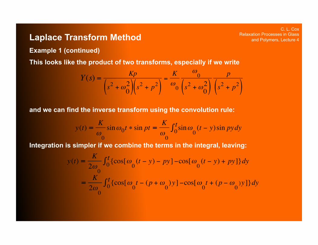
and Polymers, Lecture 4 Laplace Transform Method Example 1 (continued)
This looks like the product of two transforms, especially if we write
and we can find the inverse transform using the convolution rule:
Integration is simpler if we combine the terms in the integral, leaving:
€
Y (s) = Kp
s2 +ω02( ) s2 + p2( )
=Kω0
ω0
s2 +ω02( )
p
s2 + p2( )
€
y(t) = Kω0
sinω0t ∗ sin pt = Kω0
sinω0(t − y) sin pydy0
t∫
€
y(t) = K2ω
0
{cos[ω0(t − y) − py] −cos[ω
0(t − y) + py]}dy0
t∫
€
= K2ω
0
{cos[ω0t − (p +ω
0)y ] −cos[ω
0t + (p − ω
0)y ]}dy0
t∫

C. L. Cox Relaxation Processes in Glass
and Polymers, Lecture 4 Laplace Transform Method Example 1 (continued)
Integrating
results in
and we’re done, UNLESS
Suppose . Then simplifying the integrand, and evaluating the integral results
in the solution
Now, instead of the superposition of two harmonic oscillations, we have the amplitude growing as t increases. This is called resonance.
€
y(t) = K2ω
0
{cos[ω0t − (p +ω
0)y] −cos[ω
0t + (p − ω
0)y]}dy0
t∫
€
y(t) = K
p2 − ω02
pω0
sinω0t − sin pt
€
p2 − ω02 = 0
€
p = ω0
€
y(t) = K
2ω02sinω
0t − ω
0t cosω
0t( )

C. L. Cox Relaxation Processes in Glass
and Polymers, Lecture 4 Laplace Transform Method Example 2: An initial value problem with variable coefficients in the differential equation
Solve this IVP:
First consider the Laplace transform of :
Similarly
So the differential equation becomes
Gathering terms results in the equation
€
t y' '+(4t − 2)y'−4y = 0y(0) =1
€
t y' '
€
L t y''{ } = −dds
L y''{ } = −dds
s 2Y − sy(0)− y'(0)
= −(2sY + s2Y '−y(0))
€
L t y'{ } = −dds
L y'{ } = −dds
sY − y(0)( ) = −Y − sY '
€
(s2 + 4s)Y '+(4s+ 8)Y = 3€
−(2sY + s2Y '−y(0)) − 4(Y + sY ') − 2(sY − y(0)) − 4Y = 0
C. L. Cox Relaxation Processes in Glass
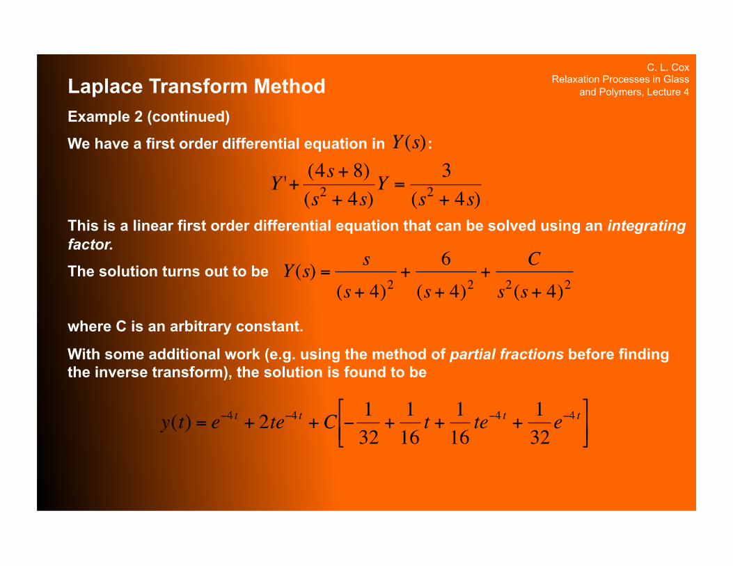
and Polymers, Lecture 4 Laplace Transform Method Example 2 (continued)
We have a first order differential equation in :
This is a linear first order differential equation that can be solved using an integrating factor.
The solution turns out to be
where C is an arbitrary constant.
With some additional work (e.g. using the method of partial fractions before finding the inverse transform), the solution is found to be
€
Y '+ (4s+ 8)(s2 + 4s)
Y =3
(s2 + 4s)€
Y (s)
€
Y (s) =s
(s+ 4)2+
6
(s+ 4)2+
C
s2(s+ 4)2
€
y(t) = e−4 t + 2te−4 t + C −132
+116t +
116te−4 t +
132e−4 t
C. L. Cox Relaxation Processes in Glass
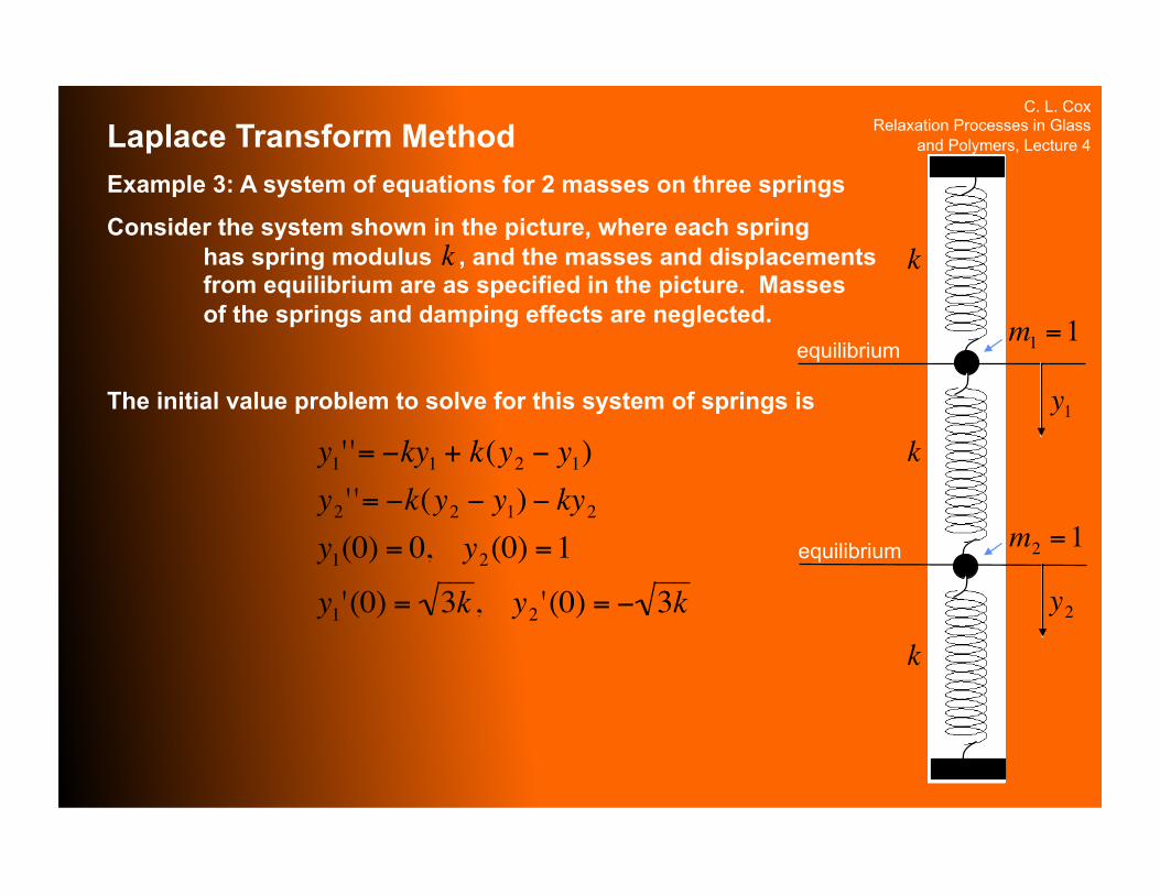
and Polymers, Lecture 4 Laplace Transform Method Example 3: A system of equations for 2 masses on three springs
Consider the system shown in the picture, where each spring has spring modulus , and the masses and displacements from equilibrium are as specified in the picture. Masses of the springs and damping effects are neglected.
The initial value problem to solve for this system of springs is
€
y1' '= −ky1 + k(y2 − y1)y2 ' '= −k(y2 − y1) − ky2y1(0) = 0, y2(0) =1
y1'(0) = 3k , y2 '(0) = − 3k
€
y1
equilibrium €
k
€
k
€
y2
equilibrium €
k
€
k
€
m1 =1
€
m2 =1
C. L. Cox Relaxation Processes in Glass
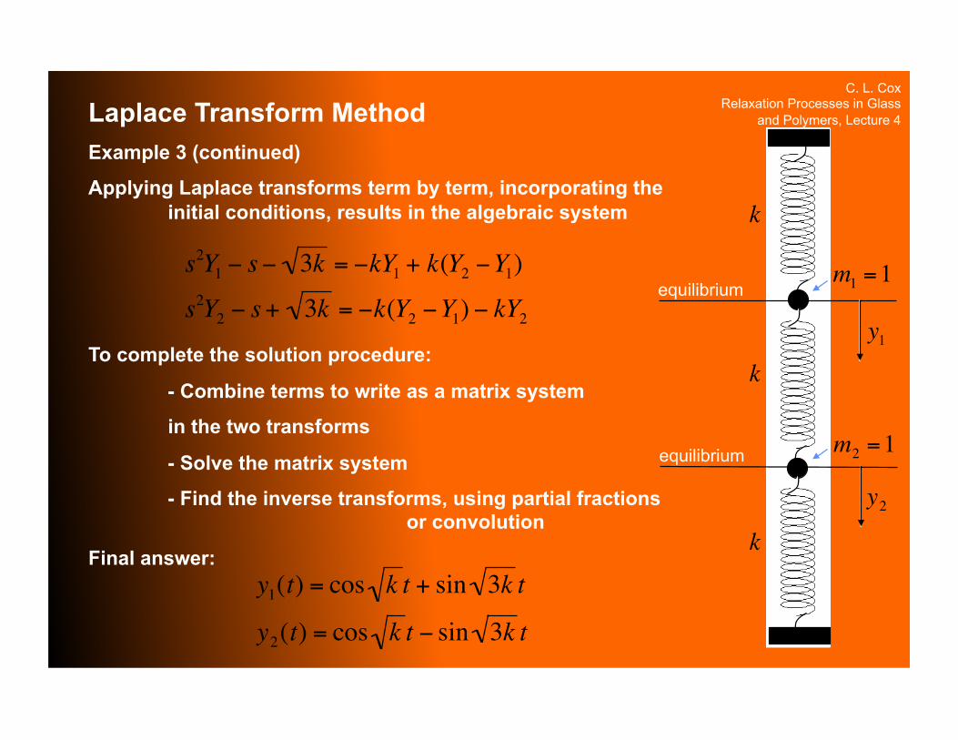
and Polymers, Lecture 4 Laplace Transform Method Example 3 (continued)
Applying Laplace transforms term by term, incorporating the initial conditions, results in the algebraic system
To complete the solution procedure:
- Combine terms to write as a matrix system
in the two transforms
- Solve the matrix system
- Find the inverse transforms, using partial fractions or convolution
Final answer:
€
s2Y1 − s− 3k = −kY1 + k(Y2 −Y1)
s2Y2 − s+ 3k = −k(Y2 −Y1) − kY2
€
y1
equilibrium €
k
€
y2
equilibrium €
k
€
k
€
m1 =1
€
m2 =1
€
y1(t) = cos k t + sin 3k t
y2(t) = cos k t − sin 3k t
C. L. Cox Relaxation Processes in Glass
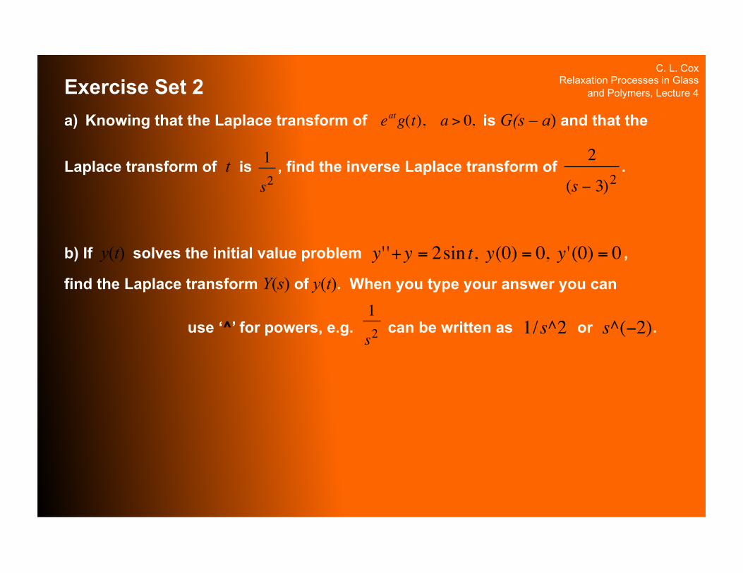
and Polymers, Lecture 4 Exercise Set 2 a) Knowing that the Laplace transform of is G(s – a) and that the
Laplace transform of t is , find the inverse Laplace transform of .
b) If y(t) solves the initial value problem ,
find the Laplace transform Y(s) of y(t). When you type your answer you can
use ‘^’ for powers, e.g. can be written as or .
€
eatg(t), a > 0,
€
1
s2
€
2
(s − 3)2
€
y' '+y = 2sin t, y(0) = 0, y'(0) = 0
€
1
s2
€
1/s^2
€
s^(−2)