Embed Size (px)
Citation preview
Statistics and Research Methodology Dr. Samir Safi
١
١
Statistics and Research Methodology
Statistics Part
By
Dr. Samir Safi
Associate Professor of Statistics
Spring 2012
١
٢٢
Lecture #1
Introduction
Numerical Descriptive Techniques
Statistics and Research Methodology Dr. Samir Safi
٢
٣
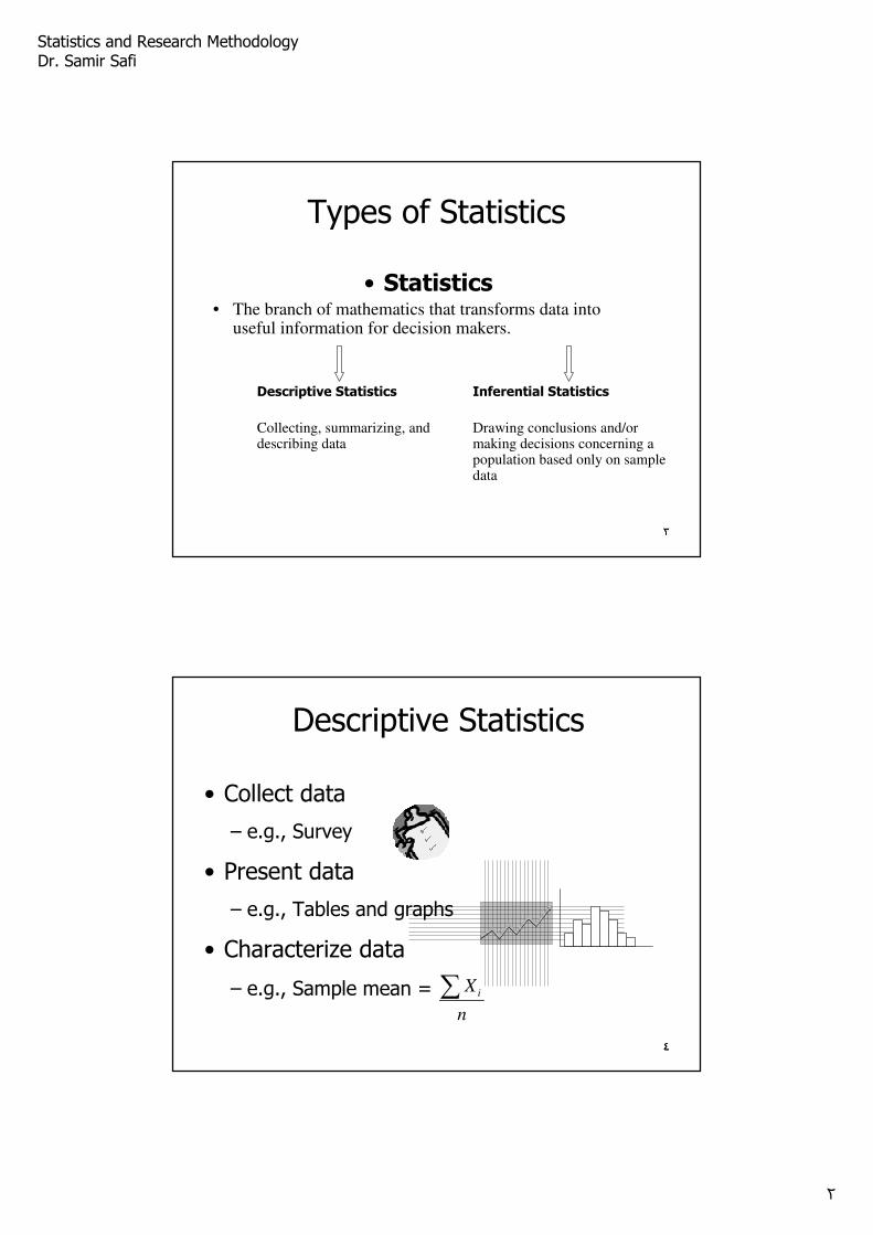
Types of Statistics
• Statistics • The branch of mathematics that transforms data into
useful information for decision makers.
Descriptive Statistics
Collecting, summarizing, and describing data
Inferential Statistics
Drawing conclusions and/or making decisions concerning a population based only on sample data
٣
٤
Descriptive Statistics
• Collect data
– e.g., Survey
• Present data
– e.g., Tables and graphs
• Characterize data
– e.g., Sample mean = iX
n
∑
٤
Statistics and Research Methodology Dr. Samir Safi
٣
٥
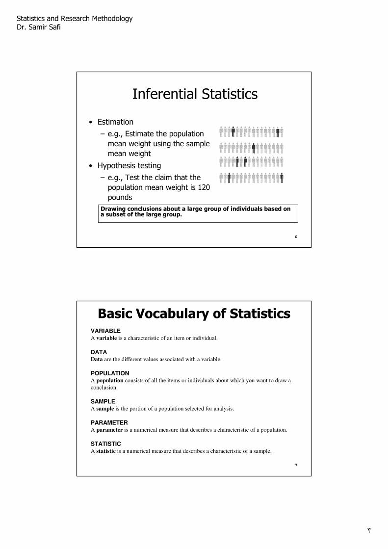
Inferential Statistics
• Estimation
– e.g., Estimate the population
mean weight using the sample
mean weight
• Hypothesis testing
– e.g., Test the claim that the
population mean weight is 120
pounds
Drawing conclusions about a large group of individuals based on a subset of the large group.
٥
٦
Basic Vocabulary of StatisticsVARIABLEA variable is a characteristic of an item or individual.
DATAData are the different values associated with a variable.
POPULATIONA population consists of all the items or individuals about which you want to draw a
conclusion.
SAMPLEA sample is the portion of a population selected for analysis.
PARAMETERA parameter is a numerical measure that describes a characteristic of a population.
STATISTICA statistic is a numerical measure that describes a characteristic of a sample.
٦
Statistics and Research Methodology Dr. Samir Safi
٤
٧٧
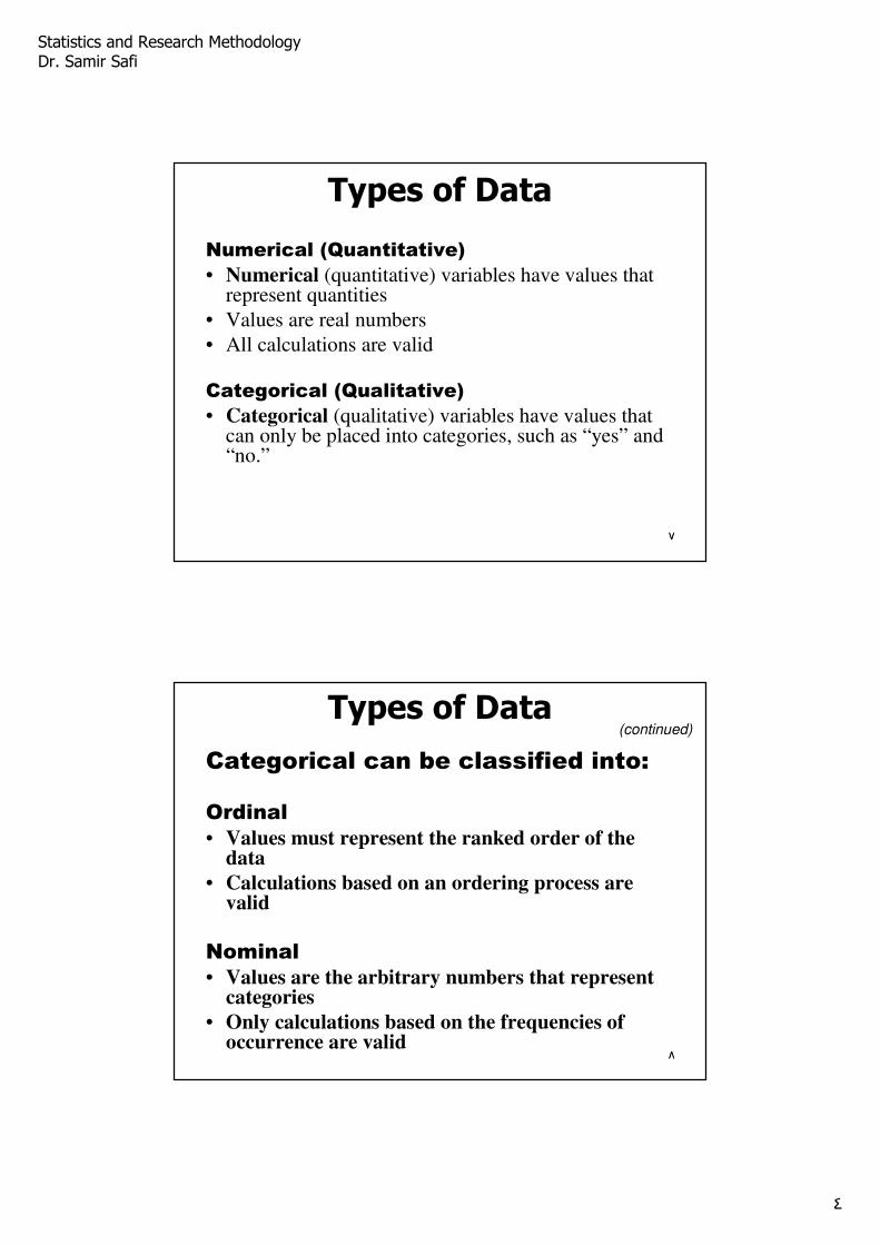
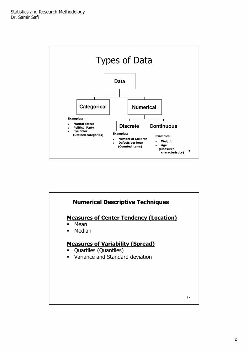
Types of Data
Numerical (Quantitative)
• Numerical (quantitative) variables have values that represent quantities
• Values are real numbers
• All calculations are valid
Categorical (Qualitative)
• Categorical (qualitative) variables have values that can only be placed into categories, such as “yes” and “no.”
٨
Types of Data
Categorical can be classified into:
Ordinal
• Values must represent the ranked order of the data
• Calculations based on an ordering process are valid
Nominal
• Values are the arbitrary numbers that represent categories
• Only calculations based on the frequencies of occurrence are valid
٨
(continued)
Statistics and Research Methodology Dr. Samir Safi
٥
٩
Types of Data
Data
Categorical Numerical
Discrete Continuous
Examples:
� Marital Status
� Political Party� Eye Color
(Defined categories) Examples:
� Number of Children
� Defects per hour
(Counted items)
Examples:
� Weight
� Age
(Measured characteristics) ٩
١٠١٠
Numerical Descriptive Techniques
Measures of Center Tendency (Location)� Mean� Median
Measures of Variability (Spread)� Quartiles (Quantiles)� Variance and Standard deviation
Statistics and Research Methodology Dr. Samir Safi
٦
١١
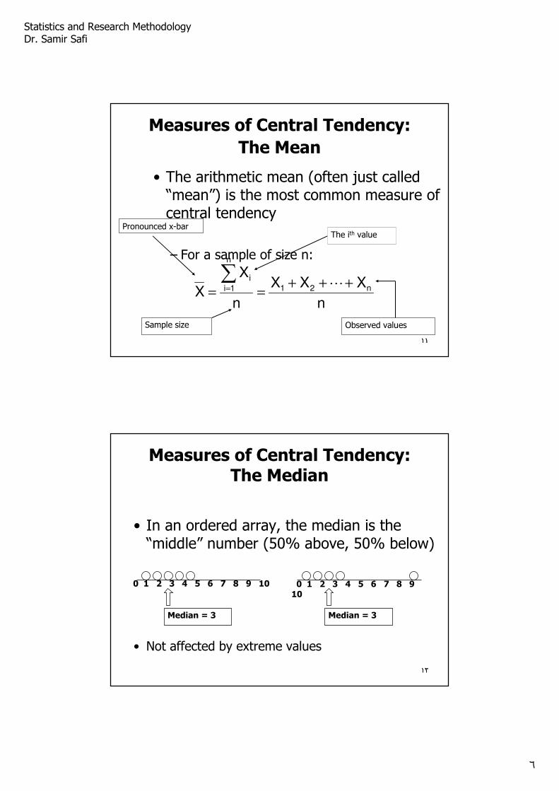
Measures of Central Tendency:
The Mean
• The arithmetic mean (often just called “mean”) is the most common measure of central tendency
– For a sample of size n:
Sample size
n
XXX
n
X
X n21
n
1ii +++
==∑
= ⋯
Observed values
The ith valuePronounced x-bar
١١
١٢
Measures of Central Tendency:The Median
• In an ordered array, the median is the “middle” number (50% above, 50% below)
• Not affected by extreme values
0 1 2 3 4 5 6 7 8 9 10
Median = 3
0 1 2 3 4 5 6 7 8 9 10
Median = 3
١٢
Statistics and Research Methodology Dr. Samir Safi
٧
١٣
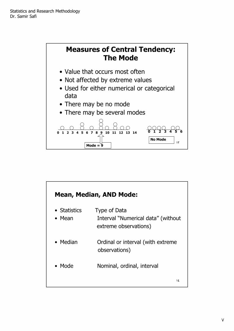
Measures of Central Tendency:The Mode
• Value that occurs most often
• Not affected by extreme values
• Used for either numerical or categorical data
• There may be no mode
• There may be several modes
0 1 2 3 4 5 6 7 8 9 10 11 12 13 14
Mode = 9
0 1 2 3 4 5 6
No Mode١٣
١٤١٤
Mean, Median, AND Mode:
• Statistics Type of Data
• Mean Interval “Numerical data” (without
extreme observations)
• Median Ordinal or interval (with extreme
observations)
• Mode Nominal, ordinal, interval
Statistics and Research Methodology Dr. Samir Safi
٨
١٥١٥
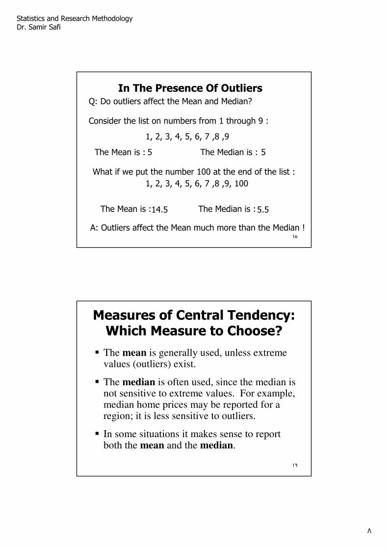
In The Presence Of OutliersQ: Do outliers affect the Mean and Median?
Consider the list on numbers from 1 through 9 :
1, 2, 3, 4, 5, 6, 7 ,8 ,9
The Mean is : 5 The Median is : 5
What if we put the number 100 at the end of the list :
The Mean is :
1, 2, 3, 4, 5, 6, 7 ,8 ,9, 100
14.5 The Median is :5.5
A: Outliers affect the Mean much more than the Median !
١٦
Measures of Central Tendency:Which Measure to Choose?
� The mean is generally used, unless extreme values (outliers) exist.
� The median is often used, since the median is not sensitive to extreme values. For example, median home prices may be reported for a region; it is less sensitive to outliers.
� In some situations it makes sense to report both the mean and the median.
١٦
Statistics and Research Methodology Dr. Samir Safi
٩
١٧Chap 3-١٧
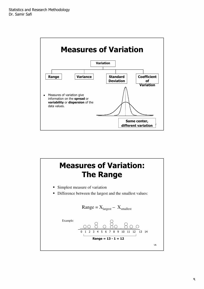
Same center,
different variation
Measures of Variation
� Measures of variation give information on the spread orvariability or dispersion of the data values.
Variation
Standard Deviation
Coefficient of
Variation
Range Variance
١٨
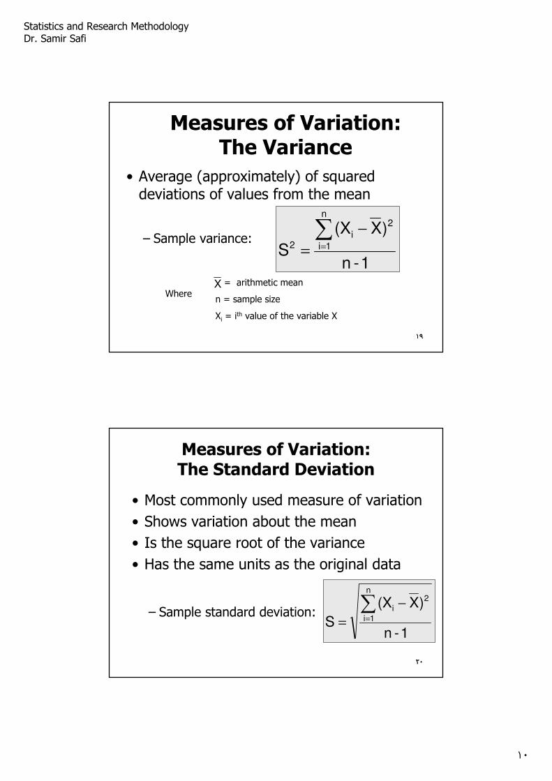
Measures of Variation:The Range
� Simplest measure of variation
� Difference between the largest and the smallest values:
Range = Xlargest – Xsmallest
0 1 2 3 4 5 6 7 8 9 10 11 12 13 14
Range = 13 - 1 = 12
Example:
١٨
Statistics and Research Methodology Dr. Samir Safi
١٠
١٩
• Average (approximately) of squared deviations of values from the mean
– Sample variance:
Measures of Variation:The Variance
1-n
)X(X
S
n
1i
2i
2∑
=
−
=
Where= arithmetic mean
n = sample size
Xi = ith value of the variable X
X
١٩
٢٠
Measures of Variation:The Standard Deviation
• Most commonly used measure of variation
• Shows variation about the mean
• Is the square root of the variance
• Has the same units as the original data
– Sample standard deviation:
1-n
)X(X
S
n
1i
2i∑
=
−
=
٢٠
Statistics and Research Methodology Dr. Samir Safi
١١
٢١
Measures of Variation:Summary Characteristics
� The more the data are spread out, the greater the range, variance, and standard deviation.
� The more the data are concentrated, the smaller the range, variance, and standard deviation.
� If the values are all the same (no variation), all these measures will be zero.
� None of these measures are ever negative.
٢١
٢٢
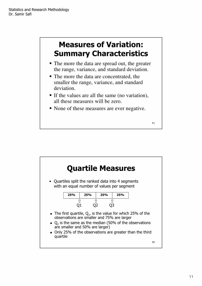
Quartile Measures
• Quartiles split the ranked data into 4 segments with an equal number of values per segment
25%
� The first quartile, Q1, is the value for which 25% of the observations are smaller and 75% are larger
� Q2 is the same as the median (50% of the observations are smaller and 50% are larger)
� Only 25% of the observations are greater than the third quartile
Q1 Q2 Q3
25% 25% 25%
٢٢
Statistics and Research Methodology Dr. Samir Safi
١٢
٢٣
Quartile Measures:The Interquartile Range (IQR)
• The IQR is Q3 – Q1 and measures the spread in the middle 50% of the data
• The IQR is also called the midspread because it covers the middle 50% of the data
• The IQR is a measure of variability that is not influenced by outliers or extreme values
• Measures like Q1, Q3, and IQR that are not influenced by outliers are called resistant measures
٢٣
٢٤
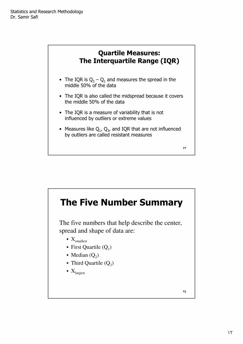
The Five Number Summary
The five numbers that help describe the center,
spread and shape of data are:
� Xsmallest
� First Quartile (Q1)
� Median (Q2)
� Third Quartile (Q3)
� Xlargest
٢٤
Statistics and Research Methodology Dr. Samir Safi
١٣
٢٥٢٥
Which Measure To Use ?
Q: When is the mean better than median? When is the five number summary better than the standard deviation?
Rules Of Thumb
A1: If outliers appear, or if your distribution is skewed, then the mean could be affected, so use the median and the five number summary.
A2: If the distribution is reasonably symmetric and is free of outliers, then the mean and standard deviationshould be used.
٢٦٢٦٢٦
Lecture #2
Introduction to Statistical Inference
• Introduction
• T-Tests
٢٦
Statistics and Research Methodology Dr. Samir Safi
١٤
٢٧٢٧٢٧
Introudction to Statistical Inference
Statistical inference involves using data collected in a sample to make statements (inferences) about unknown population parameters.
Two types of statistical inference are:• estimation of parameters (Point and Confidence estimation).• statistical tests about parameters (Testing Hypothesis).
٢٧
٢٨٢٨٢٨
Tests of Significance
There are two common types of formal statistical inference:
1) Confidence intervals
• They are appropriate when our goal is toestimate a population parameter.
2) Hypothesis Testing
• To assess the evidence provided by the datain favor of some claim about the population.
٢٨
Statistics and Research Methodology Dr. Samir Safi
١٥
٢٩٢٩
General Terms: Hypotheses :What is a
Hypothesis?
• A hypothesis is a claim (assertion) about a population parameter:
- population mean
–population proportion
Example: The mean monthly cell phone bill in this city is µ = $42
Example: The proportion of adults in this city with cell phones is π = 0.68
٢٩
٣٠٣٠٣٠
General Terms: Hypotheses
The null hypothesis, denoted by H0, is a conjecture about a population parameter that is presumed to be true. It is usually a statement of no effect or no change.
Example: The population is all students taking the Research Methodology. The parameter of interest is the mean Research Methodology score. ( µµµµ = mean Methodology score)
Suppose we believe that the mean Methodology score is 75.
Then H0: µ µ µ µ = 75
٣٠
Statistics and Research Methodology Dr. Samir Safi
١٦
٣١٣١
The Null Hypothesis, H0
• Begin with the assumption that the null hypothesis is true
–Similar to the notion of innocent until proven guilty
• Always contains “=” , “≤” or “≥≥≥≥” sign
• May or may not be rejected
(continued)
٣١
٣٢٣٢٣٢
General Terms and Characteristics
The alternative (or research) hypothesis, denoted by Ha or H1, is a conjecture about a population parameter that the researcher suspects or hopes is true.
Example: A new course has been developed which will hopefully improve students scores on the Research Methodology. We want to test to see if there is an improvement.
Then Ha: µ > 75
٣٢
Statistics and Research Methodology Dr. Samir Safi
١٧
٣٣٣٣
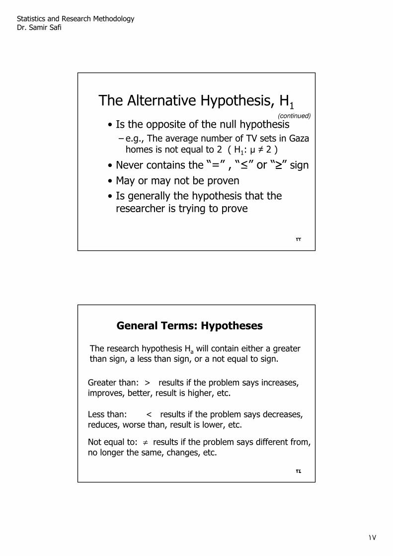
The Alternative Hypothesis, H1
• Is the opposite of the null hypothesis
– e.g., The average number of TV sets in Gaza homes is not equal to 2 ( H1: µ ≠ 2 )
• Never contains the “=” , “≤” or “≥≥≥≥” sign
• May or may not be proven
• Is generally the hypothesis that the researcher is trying to prove
(continued)
٣٣
٣٤٣٤٣٤
The research hypothesis Ha will contain either a greater than sign, a less than sign, or a not equal to sign.
Greater than: > results if the problem says increases, improves, better, result is higher, etc.
Less than: < results if the problem says decreases, reduces, worse than, result is lower, etc.
Not equal to: ≠ results if the problem says different from,
no longer the same, changes, etc.
General Terms: Hypotheses
٣٤
Statistics and Research Methodology Dr. Samir Safi
١٨
٣٥٣٥٣٥
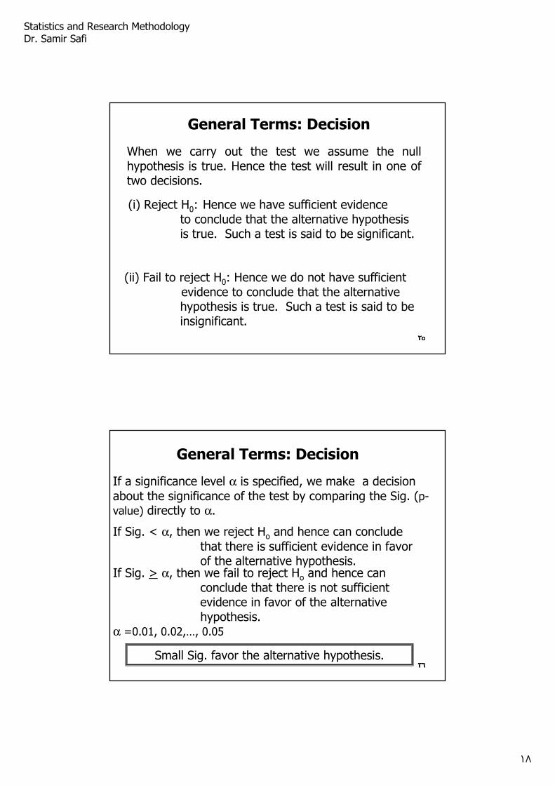
General Terms: Decision
When we carry out the test we assume the null hypothesis is true. Hence the test will result in one of two decisions.
(i) Reject H0: Hence we have sufficient evidence to conclude that the alternative hypothesisis true. Such a test is said to be significant.
(ii) Fail to reject H0: Hence we do not have sufficientevidence to conclude that the alternativehypothesis is true. Such a test is said to beinsignificant.
٣٥
٣٦٣٦٣٦
General Terms: Decision
If a significance level α is specified, we make a decision
about the significance of the test by comparing the Sig. (p-
value) directly to α.
If Sig. < α, then we reject Ho and hence can conclude
that there is sufficient evidence in favorof the alternative hypothesis.
If Sig. > α, then we fail to reject Ho and hence canconclude that there is not sufficientevidence in favor of the alternativehypothesis.
α =0.01, 0.02,…, 0.05
Small Sig. favor the alternative hypothesis.٣٦
Statistics and Research Methodology Dr. Samir Safi
١٩
٣٧٣٧٣٧
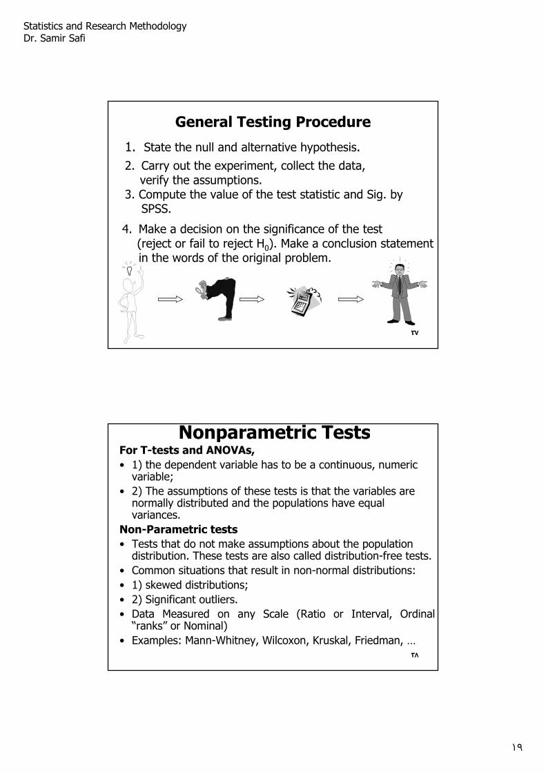
General Testing Procedure
1. State the null and alternative hypothesis.
2. Carry out the experiment, collect the data,verify the assumptions.
3. Compute the value of the test statistic and Sig. by SPSS.
4. Make a decision on the significance of the test(reject or fail to reject H0). Make a conclusion statement in the words of the original problem.
٣٧
٣٨
Nonparametric TestsFor T-tests and ANOVAs,
• 1) the dependent variable has to be a continuous, numeric variable;
• 2) The assumptions of these tests is that the variables are normally distributed and the populations have equal variances.
Non-Parametric tests
• Tests that do not make assumptions about the population distribution. These tests are also called distribution-free tests.
• Common situations that result in non-normal distributions:
• 1) skewed distributions;
• 2) Significant outliers.
• Data Measured on any Scale (Ratio or Interval, Ordinal “ranks” or Nominal)
• Examples: Mann-Whitney, Wilcoxon, Kruskal, Friedman, …٣٨٣٨
Statistics and Research Methodology Dr. Samir Safi
٢٠
٣٩٣٩
Choosing Between Parametric And Nonparametric Tests
• Definitely choose a parametric test if you are sure that your data were sampled from a population that follows a Normal distribution (at least approximately).
• Definitely select a nonparametric test if the outcome is a rank or a score and the population is clearly not Normal. e.g class ranking of students, or a Likert scale “Strongly disagree (1), disagree (2), Neutral (3), Agree (4), Strongly agree (5)”.
٣٩
٤٠
Normality Test
• We can examine the normality assumption both graphically and by use a formal statistical test.
• The Kolmogorov-Smirnov and Shapiro-Wilk tests assess whether there is a significant departure from normality in the population distribution for the interested data.
• The Lilliefors correction is appropriate when the mean and variance are estimated from the data.
• The Shapiro-Wilks test is more sensitive to outliers in the data and is computer only when the sample size is less than 50.
• The Kolmogorov-Smirnov test is used when the sample size is at least 50 .
• For normality test, the null Hypothesis states that the population distribution is normal.
•
٤٠
Statistics and Research Methodology Dr. Samir Safi
٢١
٤١
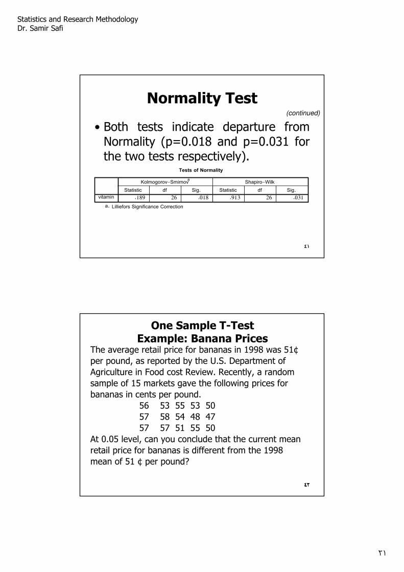
Normality Test
• Both tests indicate departure from Normality (p=0.018 and p=0.031 for the two tests respectively).
٤١
(continued)
Tests of Normality
.189 26 .018 .913 26 .031vitaminStatistic df Sig. Statistic df Sig.
Kolmogorov-Smirnova
Shapiro-Wilk
Lilliefors Significance Correctiona.
٤٢٤٢٤٢
One Sample T-TestExample: Banana Prices
The average retail price for bananas in 1998 was 51¢
per pound, as reported by the U.S. Department of
Agriculture in Food cost Review. Recently, a random
sample of 15 markets gave the following prices for
bananas in cents per pound.
56 53 55 53 50
57 58 54 48 47
57 57 51 55 50
At 0.05 level, can you conclude that the current mean
retail price for bananas is different from the 1998
mean of 51 ¢ per pound?
٤٢
Statistics and Research Methodology Dr. Samir Safi
٢٢
٤٣٤٣٤٣
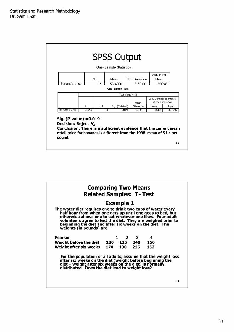
SPSS OutputOne-Sample Statistics
15 53.4000 3.50102 .90396Banana's priceN Mean Std. Deviation
Std. ErrorMean
One-Sample Test
2.655 14 .019 2.40000 .4612 4.3388Banana's pricet df Sig. (2-tailed)
MeanDifference Lower Upper
95% Confidence Intervalof the Difference
Test Value = 51
Sig. (P-value) =0.019Decision: Reject H0
Conclusion: There is a sufficient evidence that the current meanretail price for bananas is different from the 1998 mean of 51 ¢ per
pound.
٤٣
٤٤٤٤٤٤
Comparing Two MeansRelated Samples: T- Test
Example 1The water diet requires one to drink two cups of water every
half hour from when one gets up until one goes to bed, but otherwise allows one to eat whatever one likes. Four adult volunteers agree to test the diet. They are weighed prior to beginning the diet and after six weeks on the diet. The weights (in pounds) are
Pearson 1 2 3 4Weight before the diet 180 125 240 150Weight after six weeks 170 130 215 152
For the population of all adults, assume that the weight loss after six weeks on the diet (weight before beginning the diet – weight after six weeks on the diet) is normally distributed. Does the diet lead to weight loss?
٤٤
Statistics and Research Methodology Dr. Samir Safi
٢٣
٤٥٤٥٤٥
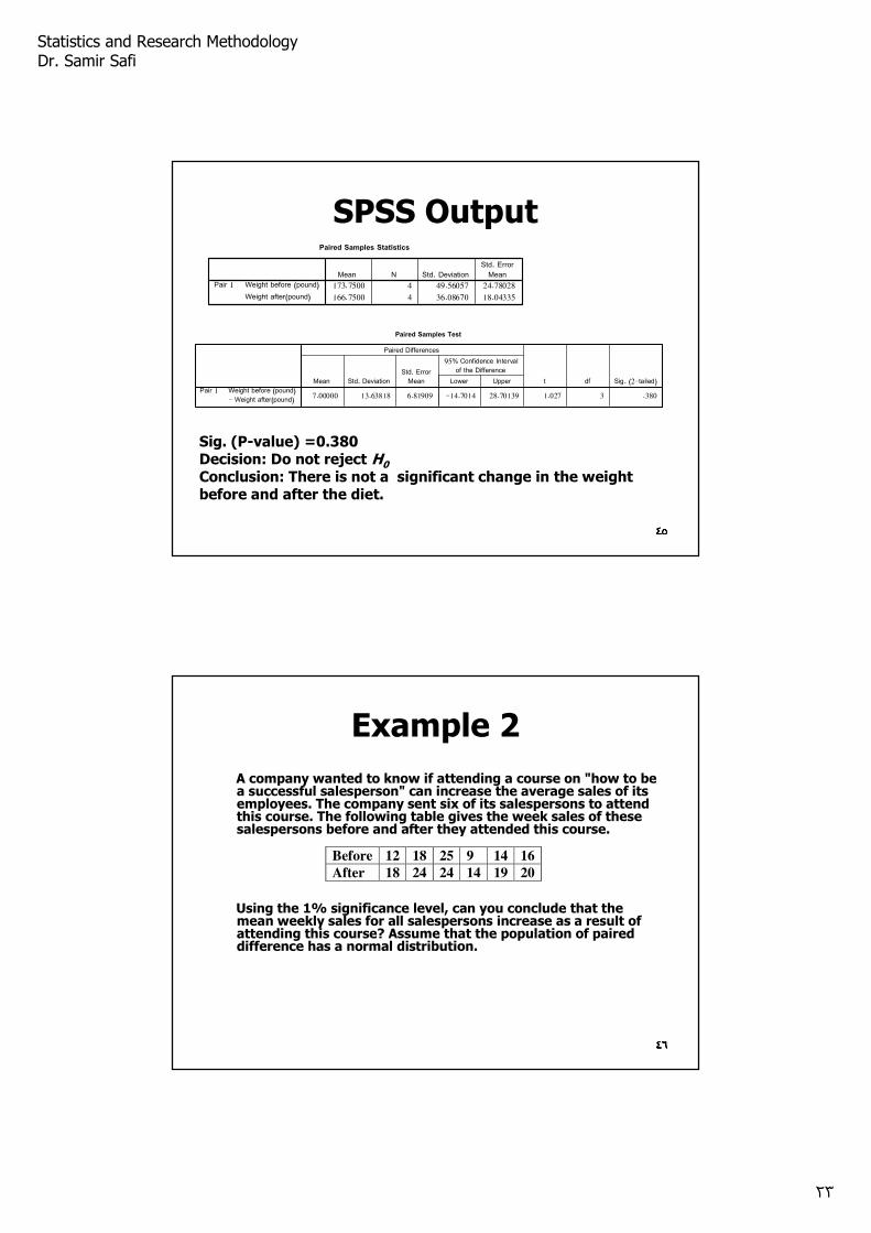
SPSS OutputPaired Samples Statistics
173.7500 4 49.56057 24.78028
166.7500 4 36.08670 18.04335
Weight before (pound)
Weight after(pound)
Pair 1Mean N Std. Deviation
Std. ErrorMean
Paired Samples Test
7.00000 13.63818 6.81909 -14.7014 28.70139 1.027 3 .380Weight before (pound)- Weight after(pound)
Pair 1Mean Std. Deviation
Std. ErrorMean Lower Upper
95% Confidence Intervalof the Difference
Paired Differences
t df Sig. (2-tailed)
Sig. (P-value) =0.380Decision: Do not reject H0
Conclusion: There is not a significant change in the weight before and after the diet.
٤٥
٤٦٤٦٤٦
Example 2
A company wanted to know if attending a course on "how to be a successful salesperson" can increase the average sales of its employees. The company sent six of its salespersons to attend this course. The following table gives the week sales of these salespersons before and after they attended this course.
Using the 1% significance level, can you conclude that the mean weekly sales for all salespersons increase as a result of attending this course? Assume that the population of paired difference has a normal distribution.
Before 12 18 25 9 14 16
After 18 24 24 14 19 20
٤٦
Statistics and Research Methodology Dr. Samir Safi
٢٤
٤٧٤٧
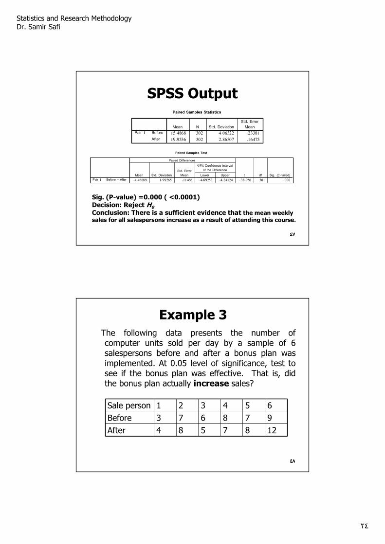
SPSS OutputPaired Samples Statistics
15.4868 302 4.06322 .23381
19.9536 302 2.86307 .16475
Before
After
Pair 1Mean N Std. Deviation
Std. ErrorMean
Paired Samples Test
-4.46689 1.99265 .11466 -4.69253 -4.24124 -38.956 301 .000Before - AfterPair 1Mean Std. Deviation
Std. ErrorMean Lower Upper
95% Confidence Intervalof the Difference
Paired Differences
t df Sig. (2-tailed)
Sig. (P-value) =0.000 ( <0.0001)Decision: Reject H0
Conclusion: There is a sufficient evidence that the mean weekly sales for all salespersons increase as a result of attending this course.
٤٧
٤٨٤٨٤٨
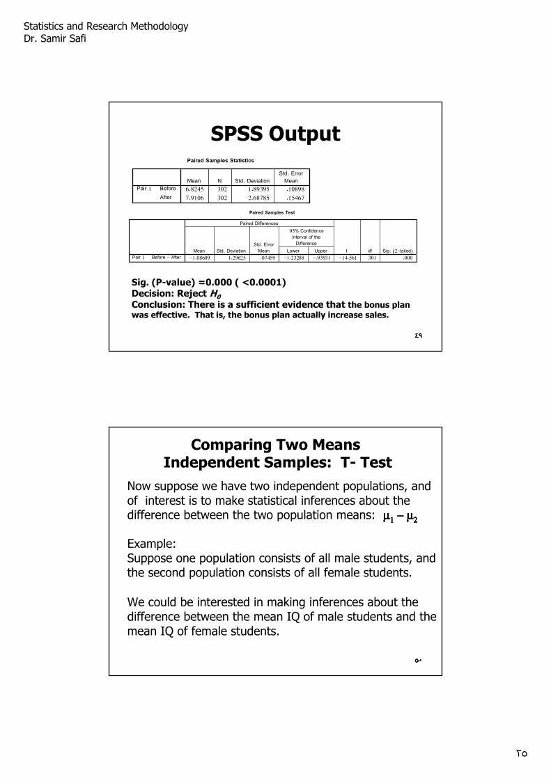
The following data presents the number of computer units sold per day by a sample of 6 salespersons before and after a bonus plan was implemented. At 0.05 level of significance, test to see if the bonus plan was effective. That is, did the bonus plan actually increase sales?
Example 3
Sale person 1 2 3 4 5 6
Before 3 7 6 8 7 9
After 4 8 5 7 8 12
٤٨
Statistics and Research Methodology Dr. Samir Safi
٢٥
٤٩٤٩
SPSS OutputPaired Samples Statistics
6.8245 302 1.89395 .10898
7.9106 302 2.68785 .15467
Before
After
Pair 1Mean N Std. Deviation
Std. ErrorMean
Paired Samples Test
-1.08609 1.29625 .07459 -1.23288 -.93931 -14.561 301 .000Before - AfterPair 1Mean Std. Deviation
Std. ErrorMean Lower Upper
95% ConfidenceInterval of the
Difference
Paired Differences
t df Sig. (2-tailed)
Sig. (P-value) =0.000 ( <0.0001)Decision: Reject H0
Conclusion: There is a sufficient evidence that the bonus plan was effective. That is, the bonus plan actually increase sales.
٤٩
٥٠٥٠٥٠
Comparing Two MeansIndependent Samples: T- Test
Now suppose we have two independent populations, and of interest is to make statistical inferences about the difference between the two population means: µµµµ1111 −−−− µµµµ2222
Example:Suppose one population consists of all male students, and the second population consists of all female students.
We could be interested in making inferences about the difference between the mean IQ of male students and the mean IQ of female students.
٥٠
Statistics and Research Methodology Dr. Samir Safi
٢٦
٥١٥١
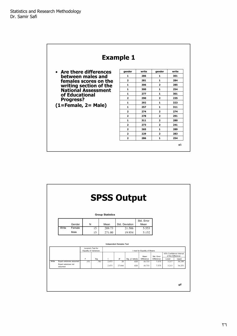
Example 1
• Are there differences between males and females scores on the writing section of the National Assessment of Educational Progress?
(1=Female, 2= Male)
gender write gender write
1 286 1 301
2 281 1 284
1 306 2 285
1 300 1 254
1 277 1 301
2 290 2 235
1 292 1 323
1 257 1 311
2 274 2 274
2 278 2 291
1 311 2 280
2 273 2 241
2 265 1 289
2 229 2 283
2 286 1 254
٥١
٥٢٥٢
SPSS Output
Group Statistics
15 289.73 21.506 5.553
15 271.00 19.954 5.152
GenderFemale
Male
WriteN Mean Std. Deviation
Std. ErrorMean
Independent Samples Test
.151 .701 2.473 28 .020 18.733 7.575 3.217 34.249
2.473 27.844 .020 18.733 7.575 3.213 34.253
Equal variances assumed
Equal variances notassumed
WriteF Sig.
Levene's Test forEquality of Variances
t df Sig. (2-tailed)Mean
DifferenceStd. ErrorDifference Lower Upper
95% Confidence Intervalof the Difference
t-test for Equality of Means
٥٢
Statistics and Research Methodology Dr. Samir Safi
٢٧
٥٣٥٣
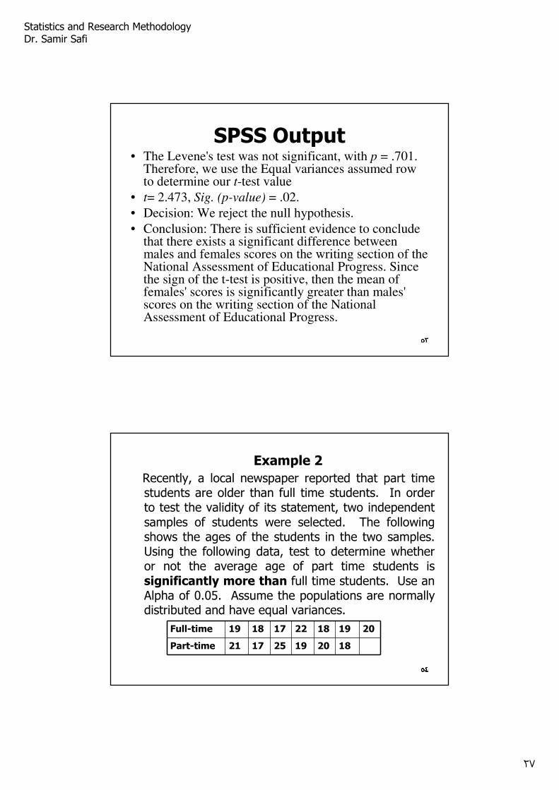
SPSS Output• The Levene's test was not significant, with p = .701.
Therefore, we use the Equal variances assumed row to determine our t-test value
• t= 2.473, Sig. (p-value) = .02.
• Decision: We reject the null hypothesis.
• Conclusion: There is sufficient evidence to conclude that there exists a significant difference between males and females scores on the writing section of the National Assessment of Educational Progress. Since the sign of the t-test is positive, then the mean of females' scores is significantly greater than males' scores on the writing section of the National Assessment of Educational Progress.
٥٣
٥٤٥٤٥٤
Example 2
Recently, a local newspaper reported that part time students are older than full time students. In order to test the validity of its statement, two independent samples of students were selected. The following shows the ages of the students in the two samples. Using the following data, test to determine whether or not the average age of part time students is significantly more than full time students. Use an Alpha of 0.05. Assume the populations are normally distributed and have equal variances.
Full-time 19 18 17 22 18 19 20
Part-time 21 17 25 19 20 18
٥٤
Statistics and Research Methodology Dr. Samir Safi
٢٨
٥٥٥٥٥٥
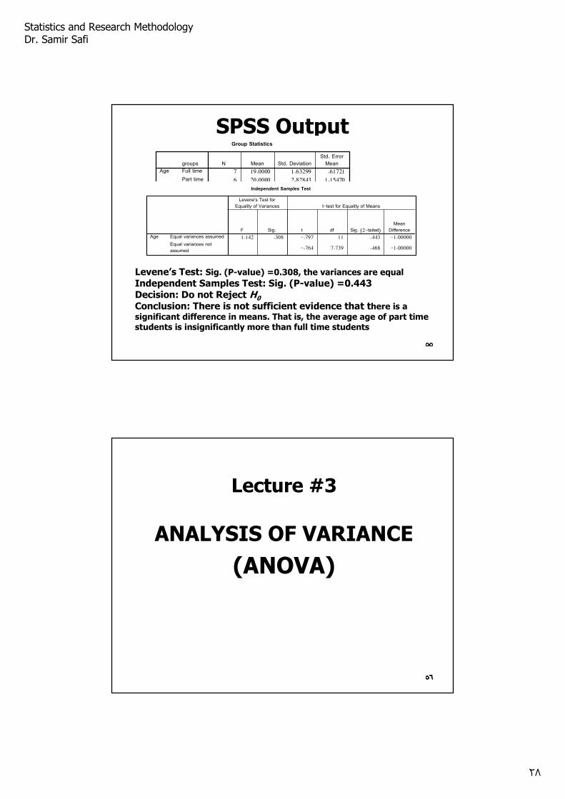
SPSS OutputGroup Statistics
7 19.0000 1.63299 .61721
6 20.0000 2.82843 1.15470
groupsFull time
Part time
AgeN Mean Std. Deviation
Std. ErrorMean
Independent Samples Test
1.142 .308 -.797 11 .443 -1.00000
-.764 7.739 .468 -1.00000
Equal variances assumed
Equal variances notassumed
AgeF Sig.
Levene's Test forEquality of Variances
t df Sig. (2-tailed)Mean
Difference
t-test for Equality of Means
Levene’s Test: Sig. (P-value) =0.308, the variances are equal
Independent Samples Test: Sig. (P-value) =0.443Decision: Do not Reject H0
Conclusion: There is not sufficient evidence that there is a significant difference in means. That is, the average age of part time students is insignificantly more than full time students
٥٥
٥٦٥٦٥٦
Lecture #3
ANALYSIS OF VARIANCE
(ANOVA)
٥٦
Statistics and Research Methodology Dr. Samir Safi
٢٩
٥٧
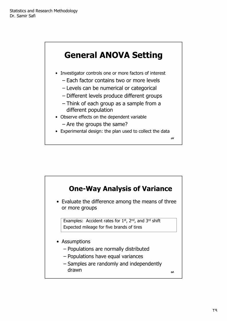
General ANOVA Setting
• Investigator controls one or more factors of interest
– Each factor contains two or more levels
– Levels can be numerical or categorical
– Different levels produce different groups
– Think of each group as a sample from a different population
• Observe effects on the dependent variable
– Are the groups the same?
• Experimental design: the plan used to collect the data
٥٧٥٧
٥٨
One-Way Analysis of Variance
• Evaluate the difference among the means of three or more groups
Examples: Accident rates for 1st, 2nd, and 3rd shift
Expected mileage for five brands of tires
• Assumptions
– Populations are normally distributed
– Populations have equal variances
– Samples are randomly and independently drawn ٥٨٥٨
Statistics and Research Methodology Dr. Samir Safi
٣٠
٥٩
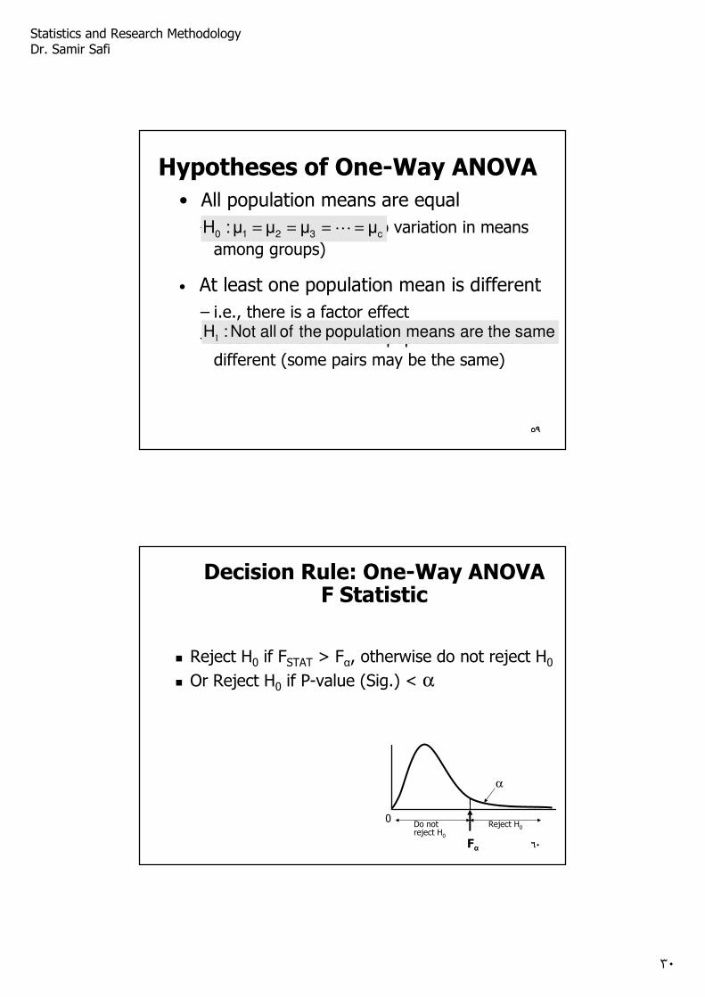
Hypotheses of One-Way ANOVA
• All population means are equal
– i.e., no factor effect (no variation in means
among groups)
• At least one population mean is different
– i.e., there is a factor effect
– Does not mean that all population means are
different (some pairs may be the same)
c3210 µµµµ:H ==== ⋯
same the are means population the of all Not:H1
٥٩
٦٠
Decision Rule: One-Way ANOVA F Statistic
� Reject H0 if FSTAT > Fα, otherwise do not reject H0
� Or Reject H0 if P-value (Sig.) < α
0
α
Reject H0Do not reject H0
Fα ٦٠
Statistics and Research Methodology Dr. Samir Safi
٣١
٦١٦١٦١
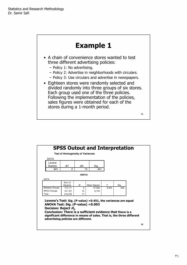
Example 1
• A chain of convenience stores wanted to test three different advertising policies:– Policy 1: No advertising.
– Policy 2: Advertise in neighborhoods with circulars.
– Policy 3: Use circulars and advertise in newspapers.
• Eighteen stores were randomly selected and divided randomly into three groups of six stores. Each group used one of the three policies. Following the implementation of the policies, sales figures were obtained for each of the stores during a 1-month period.
٦١
٦٢٦٢٦٢
SPSS Output and InterpretationTest of Homogeneity of Variances
DATA
.841 2 15 .451
Levene
Statistic df1 df2 Sig.
ANOVA
DATA
115.111 2 57.556 8.534 .003
101.167 15 6.744
216.278 17
Between Groups
Within Groups
Total
Sum ofSquares df Mean Square F Sig.
Levene’s Test: Sig. (P-value) =0.451, the variances are equal
ANOVA Test: Sig. (P-value) =0.003Decision: Reject H0
Conclusion: There is a sufficient evidence that there is a significant difference in means of sales. That is, the three different advertising policies are different.
٦٢
Statistics and Research Methodology Dr. Samir Safi
٣٢
٦٣٦٣٦٣
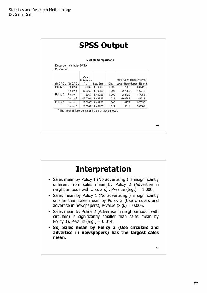
SPSS Output
Multiple Comparisons
Dependent Variable: DATA
Bonferroni
-.6667 1.49938 1.000 -4.7056 3.3723
-5.6667* 1.49938 .005 -9.7056 -1.6277
.6667 1.49938 1.000 -3.3723 4.7056
-5.0000* 1.49938 .014 -9.0389 -.9611
5.6667* 1.49938 .005 1.6277 9.7056
5.0000* 1.49938 .014 .9611 9.0389
(J) GROUPPolicy 2
Policy 3
Policy 1
Policy 3
Policy 1
Policy 2
(I) GROUPPolicy 1
Policy 2
Policy 3
MeanDifference
(I-J) Std. Error Sig. Lower BoundUpper Bound
95% Confidence Interval
The mean difference is significant at the .05 level.*.
٦٣
٦٤
Interpretation
٦٤
• Sales mean by Policy 1 (No advertising ) is insignificantly different from sales mean by Policy 2 (Advertise in neighborhoods with circulars) , P-value (Sig.) = 1.000.
• Sales mean by Policy 1 (No advertising ) is significantly smaller than sales mean by Policy 3 (Use circulars and advertise in newspapers), P-value (Sig.) = 0.005.
• Sales mean by Policy 2 (Advertise in neighborhoods with circulars) is significantly smaller than sales mean by Policy 3), P-value (Sig.) = 0.014.
• So, Sales mean by Policy 3 (Use circulars and advertise in newspapers) has the largest sales mean.
٦٤
Statistics and Research Methodology Dr. Samir Safi
٣٣
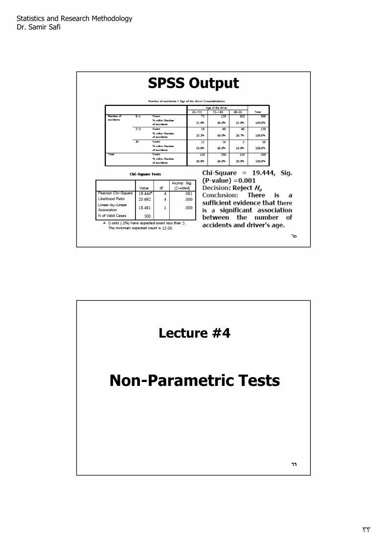
٦٥
SPSS Output
٦٥
٦٦٦٦٦٦
Lecture #4
Non-Parametric Tests
٦٦
Statistics and Research Methodology Dr. Samir Safi
٣٤
٦٧
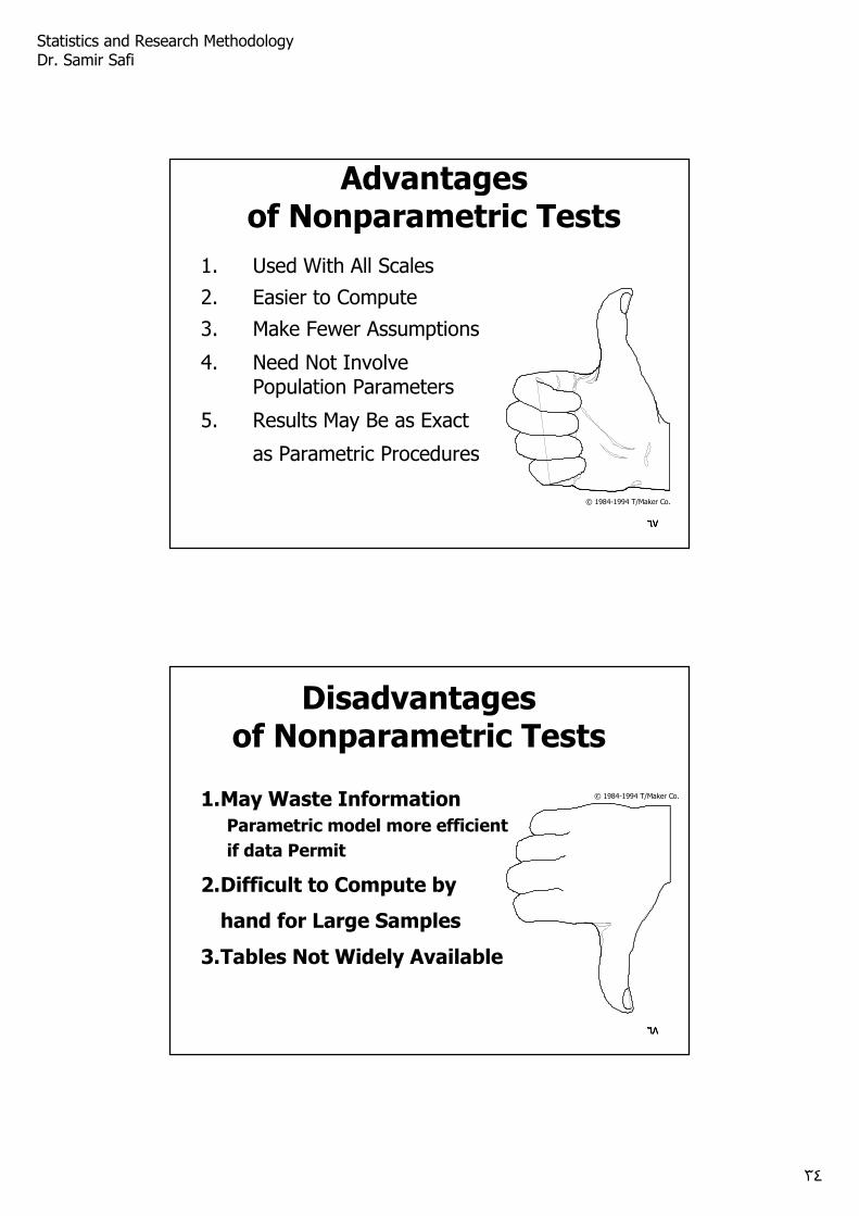
Advantages of Nonparametric Tests
1. Used With All Scales
2. Easier to Compute
3. Make Fewer Assumptions
4. Need Not Involve Population Parameters
5. Results May Be as Exact
as Parametric Procedures
© 1984-1994 T/Maker Co.
٦٧٦٧
٦٨
Disadvantages of Nonparametric Tests
1.May Waste Information
Parametric model more efficient
if data Permit
2.Difficult to Compute by
hand for Large Samples
3.Tables Not Widely Available
© 1984-1994 T/Maker Co.
٦٨٦٨
Statistics and Research Methodology Dr. Samir Safi
٣٥
٦٩٦٩
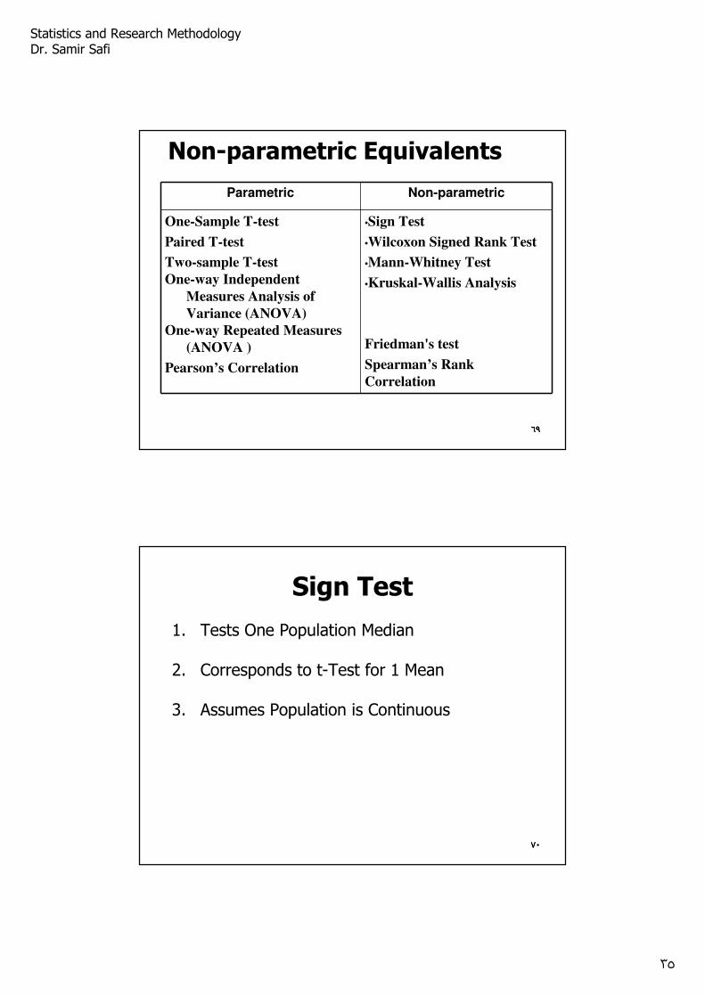
Non-parametric Equivalents
Parametric Non-parametric
One-Sample T-test
Paired T-test
Two-sample T-test
One-way Independent
Measures Analysis of
Variance (ANOVA)
One-way Repeated Measures
(ANOVA )
Pearson’s Correlation
•Sign Test
•Wilcoxon Signed Rank Test
•Mann-Whitney Test
•Kruskal-Wallis Analysis
Friedman's test
Spearman’s Rank
Correlation
٦٩
٧٠
Sign Test
1. Tests One Population Median
2. Corresponds to t-Test for 1 Mean
3. Assumes Population is Continuous
٧٠٧٠
Statistics and Research Methodology Dr. Samir Safi
٣٦
٧١
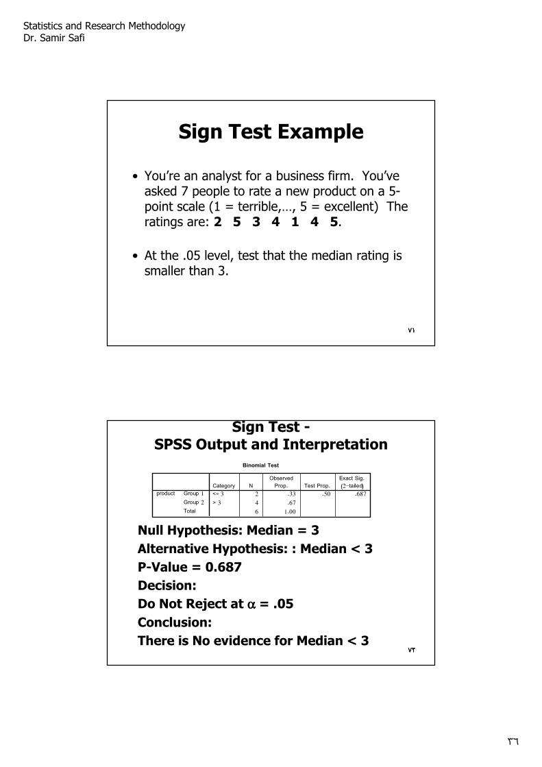
Sign Test Example
• You’re an analyst for a business firm. You’ve asked 7 people to rate a new product on a 5-point scale (1 = terrible,…, 5 = excellent) The ratings are: 2 5 3 4 1 4 5.
• At the .05 level, test that the median rating is smaller than 3.
٧١٧١
٧٢
Sign Test -SPSS Output and Interpretation
Null Hypothesis: Median = 3
Alternative Hypothesis: : Median < 3
P-Value = 0.687
Decision:
Do Not Reject at αααα = .05
Conclusion:
There is No evidence for Median < 3
Binomial Test
<= 3 2 .33 .50 .687
> 3 4 .67
6 1.00
Group 1
Group 2
Total
productCategory N
ObservedProp. Test Prop.
Exact Sig.(2-tailed)
٧٢٧٢
Statistics and Research Methodology Dr. Samir Safi
٣٧
٧٣
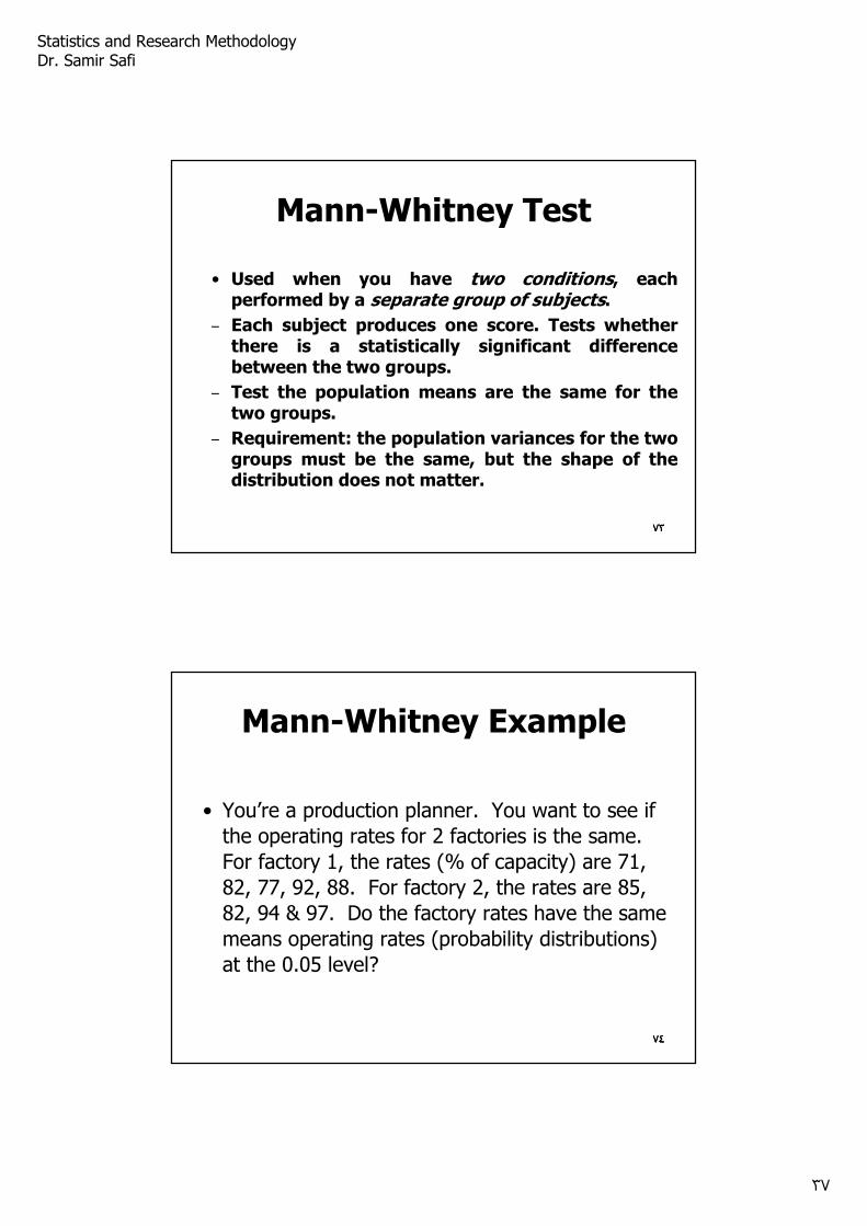
Mann-Whitney Test
• Used when you have two conditions, each performed by a separate group of subjects.
– Each subject produces one score. Tests whether there is a statistically significant difference between the two groups.
– Test the population means are the same for the two groups.
– Requirement: the population variances for the two groups must be the same, but the shape of the distribution does not matter.
٧٣٧٣
٧٤
Mann-Whitney Example
• You’re a production planner. You want to see if
the operating rates for 2 factories is the same.
For factory 1, the rates (% of capacity) are 71,
82, 77, 92, 88. For factory 2, the rates are 85,
82, 94 & 97. Do the factory rates have the same
means operating rates (probability distributions)
at the 0.05 level?
٧٤٧٤
Statistics and Research Methodology Dr. Samir Safi
٣٨
٧٥
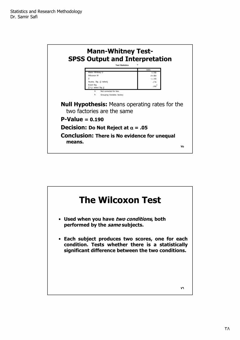
Mann-Whitney Test-SPSS Output and Interpretation
Null Hypothesis: Means operating rates for the two factories are the same
P-Value = 0.190
Decision: Do Not Reject at αααα = .05
Conclusion: There is No evidence for unequal
means.
Test Statistics b
4.500
19.500
-1.353
.176
.190a
Mann-Whitney U
Wilcoxon W
Z
Asymp. Sig. (2-tailed)
Exact Sig.[2*(1-tailed Sig.)]
rates
Not corrected for ties.a.
Grouping Variable: factoryb.
٧٥٧٥
٧٦
The Wilcoxon Test
• Used when you have two conditions, both performed by the same subjects.
• Each subject produces two scores, one for each condition. Tests whether there is a statistically significant difference between the two conditions.
٧٦٧٦
Statistics and Research Methodology Dr. Samir Safi
٣٩
٧٧
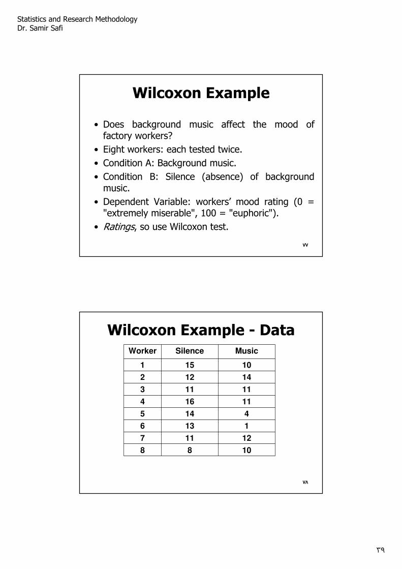
Wilcoxon Example
• Does background music affect the mood of factory workers?
• Eight workers: each tested twice.
• Condition A: Background music.
• Condition B: Silence (absence) of background music.
• Dependent Variable: workers’ mood rating (0 = "extremely miserable", 100 = "euphoric").
• Ratings, so use Wilcoxon test.
٧٧٧٧
٧٨
Wilcoxon Example - Data
Worker Silence Music
1 15 10
2 12 14
3 11 11
4 16 11
5 14 4
6 13 1
7 11 12
8 8 10
٧٨٧٨
Statistics and Research Methodology Dr. Samir Safi
٤٠
٧٩
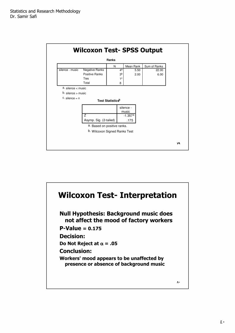
Wilcoxon Test- SPSS Output
Ranks
4a 5.50 22.00
3b 2.00 6.00
1c
8
Negative Ranks
Positive Ranks
Ties
Total
silence - musicN Mean Rank Sum of Ranks
silence < musica.
silence > musicb.
silence = musicc. Test Statisticsb
-1.357a
.175
Z
Asymp. Sig. (2-tailed)
silence -music
Based on positive ranks.a.
Wilcoxon Signed Ranks Testb.
٧٩٧٩
٨٠
Wilcoxon Test- Interpretation
Null Hypothesis: Background music does not affect the mood of factory workers
P-Value = 0.175
Decision:
Do Not Reject at αααα = .05
Conclusion:
Workers' mood appears to be unaffected by presence or absence of background music
٨٠٨٠
Statistics and Research Methodology Dr. Samir Safi
٤١
٨١
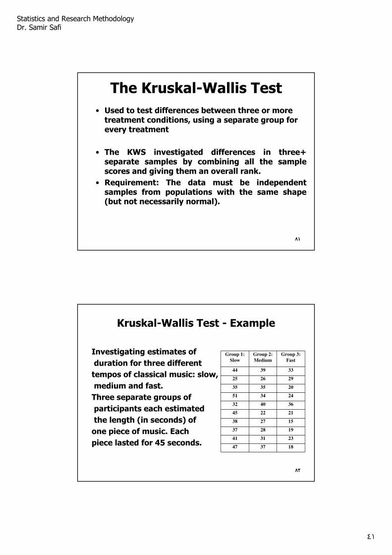
The Kruskal-Wallis Test
• Used to test differences between three or more treatment conditions, using a separate group for every treatment
• The KWS investigated differences in three+ separate samples by combining all the sample scores and giving them an overall rank.
• Requirement: The data must be independent samples from populations with the same shape (but not necessarily normal).
٨١٨١
٨٢
Kruskal-Wallis Test - Example
Investigating estimates of
duration for three different
tempos of classical music: slow,
medium and fast.
Three separate groups of
participants each estimated
the length (in seconds) of
one piece of music. Each
piece lasted for 45 seconds.
Group 1:
Slow
Group 2:
Medium
Group 3:
Fast
44 39 33
25 26 29
35 35 20
51 34 24
32 40 36
45 22 21
38 27 15
37 28 19
41 31 23
47 37 18
٨٢٨٢
Statistics and Research Methodology Dr. Samir Safi
٤٢
٨٣
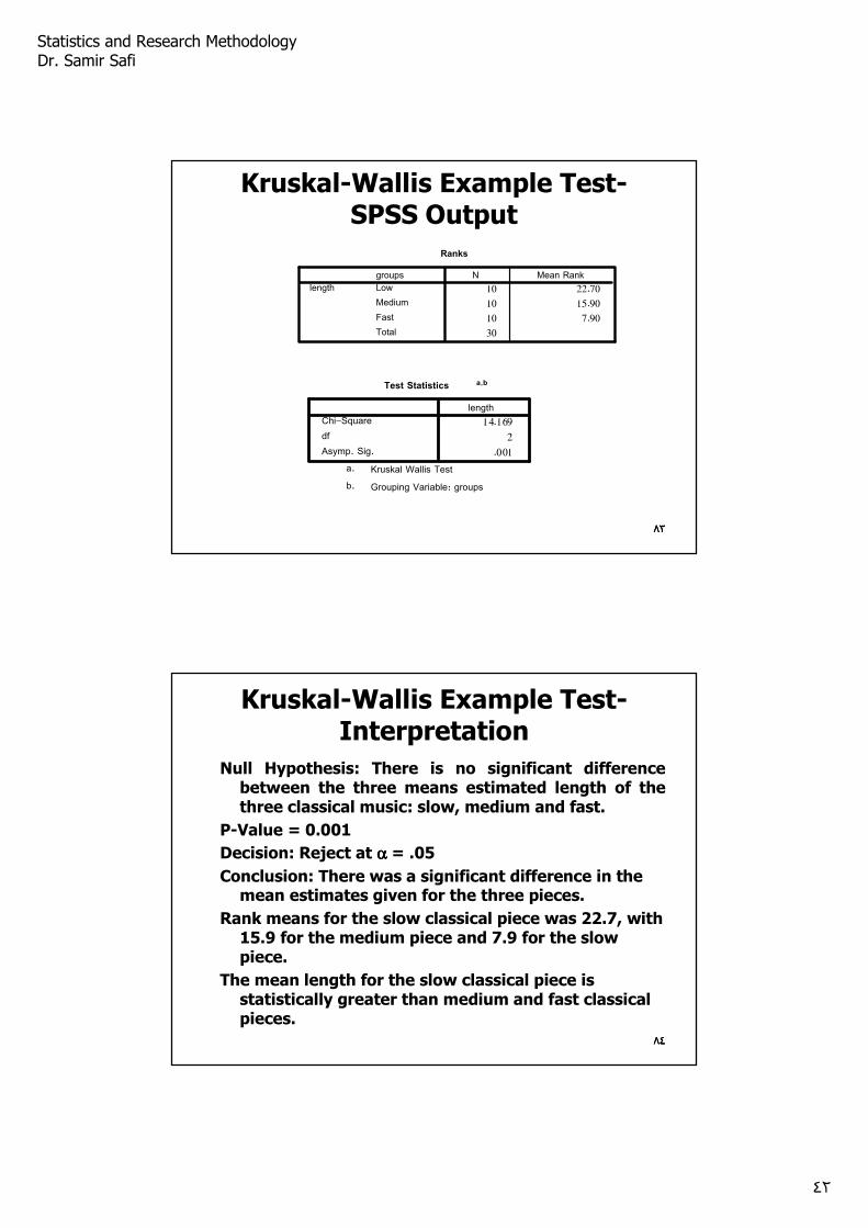
Kruskal-Wallis Example Test-SPSS Output
Ranks
10 22.70
10 15.90
10 7.90
30
groupsLow
Medium
Fast
Total
lengthN Mean Rank
Test Statistics a,b
14.169
2
.001
Chi-Square
df
Asymp. Sig.
length
Kruskal Wallis Testa.
Grouping Variable: groupsb.
٨٣٨٣
٨٤
Kruskal-Wallis Example Test-Interpretation
Null Hypothesis: There is no significant difference between the three means estimated length of the three classical music: slow, medium and fast.
P-Value = 0.001
Decision: Reject at αααα = .05
Conclusion: There was a significant difference in the mean estimates given for the three pieces.
Rank means for the slow classical piece was 22.7, with 15.9 for the medium piece and 7.9 for the slow piece.
The mean length for the slow classical piece is statistically greater than medium and fast classical pieces.
٨٤٨٤
Statistics and Research Methodology Dr. Samir Safi
٤٣
٨٥
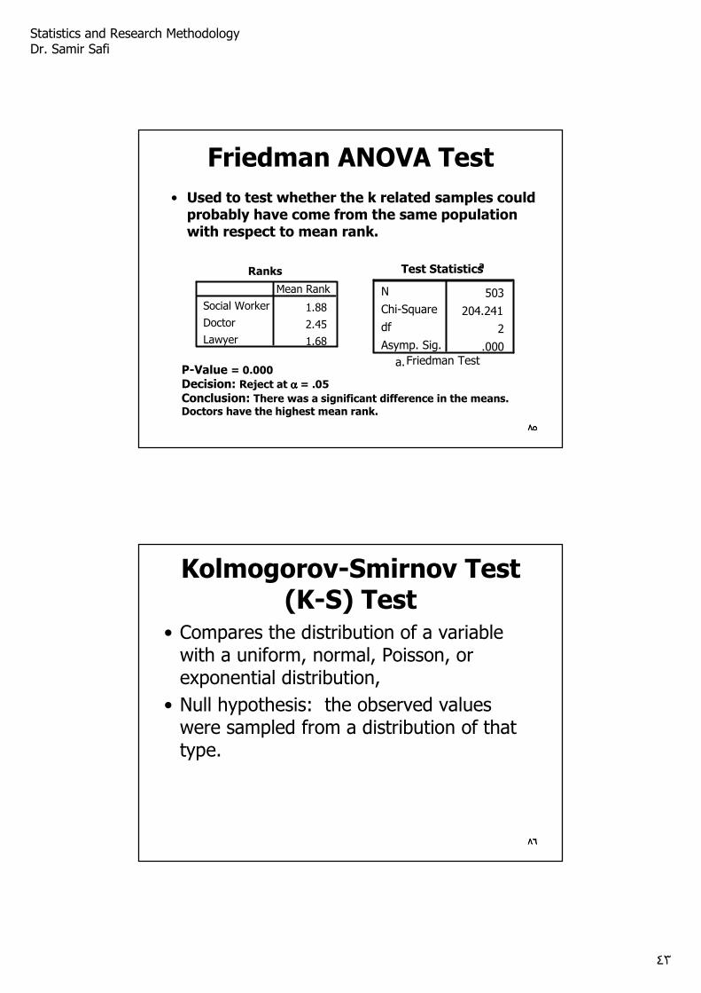
Friedman ANOVA Test
• Used to test whether the k related samples could probably have come from the same population with respect to mean rank.
٨٥
Ranks
1.88
2.45
1.68
Social Worker
Doctor
Lawyer
Mean Rank
Test Statisticsa
503
204.241
2
.000
N
Chi-Square
df
Asymp. Sig.
Friedman Testa. P-Value = 0.000
Decision: Reject at αααα = .05
Conclusion: There was a significant difference in the means. Doctors have the highest mean rank.
٨٥
٨٦
Kolmogorov-Smirnov Test(K-S) Test
• Compares the distribution of a variable with a uniform, normal, Poisson, or exponential distribution,
• Null hypothesis: the observed values were sampled from a distribution of that type.
٨٦٨٦
Statistics and Research Methodology Dr. Samir Safi
٤٤
٨٧
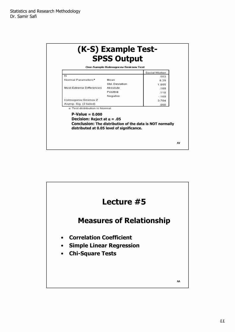
(K-S) Example Test-SPSS Output
P-Value = 0.000
Decision: Reject at αααα = .05
Conclusion: The distribution of the data is NOT normally distributed at 0.05 level of significance.
٨٧٨٧
٨٨٨٨
Lecture #5
Measures of Relationship
• Correlation Coefficient
• Simple Linear Regression
• Chi-Square Tests
٨٨
Statistics and Research Methodology Dr. Samir Safi
٤٥
٨٩٨٩
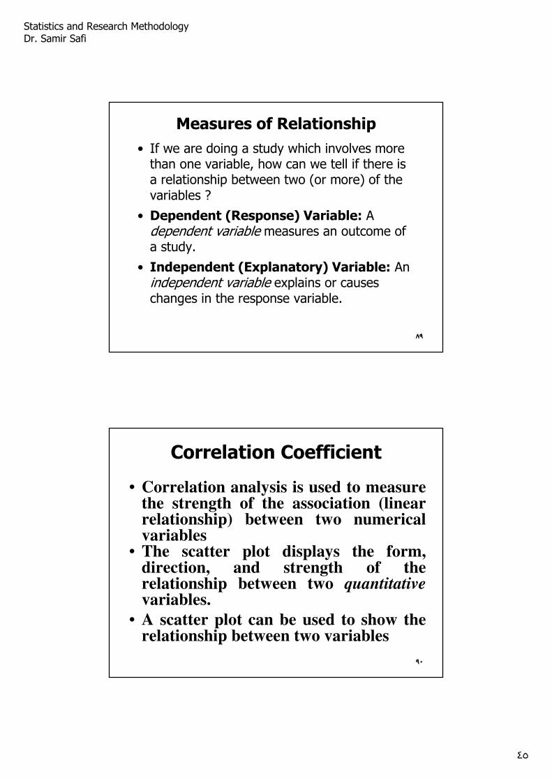
Measures of Relationship
• If we are doing a study which involves more than one variable, how can we tell if there is a relationship between two (or more) of the variables ?
• Dependent (Response) Variable: A dependent variable measures an outcome of a study.
• Independent (Explanatory) Variable: An independent variable explains or causes changes in the response variable.
٨٩
٩٠٩٠
Correlation Coefficient
• Correlation analysis is used to measure the strength of the association (linear relationship) between two numerical variables
• The scatter plot displays the form, direction, and strength of the relationship between two quantitativevariables.
• A scatter plot can be used to show the relationship between two variables
٩٠
Statistics and Research Methodology Dr. Samir Safi
٤٦
٩١٩١
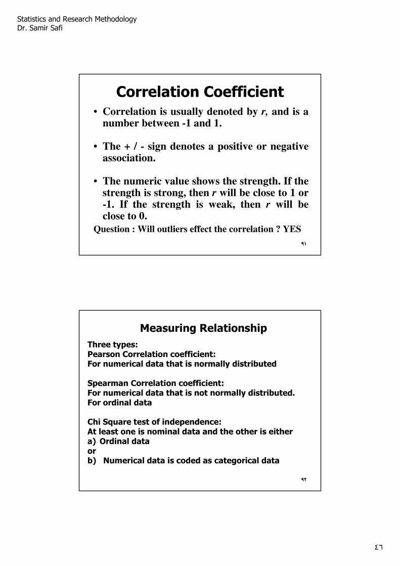
Correlation Coefficient• Correlation is usually denoted by r, and is a
number between -1 and 1.
• The + / - sign denotes a positive or negative association.
• The numeric value shows the strength. If the strength is strong, then r will be close to 1 or -1. If the strength is weak, then r will be close to 0.
Question : Will outliers effect the correlation ? YES
٩١
٩٢٩٢
Measuring Relationship
Three types:Pearson Correlation coefficient:For numerical data that is normally distributed
Spearman Correlation coefficient:For numerical data that is not normally distributed.For ordinal data
Chi Square test of independence:At least one is nominal data and the other is eithera) Ordinal dataorb) Numerical data is coded as categorical data
٩٢
Statistics and Research Methodology Dr. Samir Safi
٤٧
٩٣
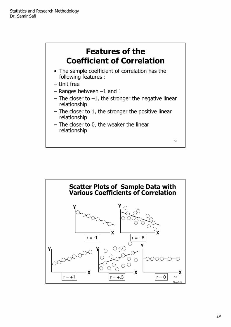
Features of theCoefficient of Correlation
• The sample coefficient of correlation has the following features :
– Unit free
– Ranges between –1 and 1
– The closer to –1, the stronger the negative linear relationship
– The closer to 1, the stronger the positive linear relationship
– The closer to 0, the weaker the linear relationship
٩٣
٩٤
Chap 3-٩٤
Scatter Plots of Sample Data with Various Coefficients of Correlation
Y
X
Y
X
Y
X
Y
X
r = -1 r = -.6
r = +.3r = +1
Y
Xr = 0 ٩٤
Statistics and Research Methodology Dr. Samir Safi
٤٨
٩٥
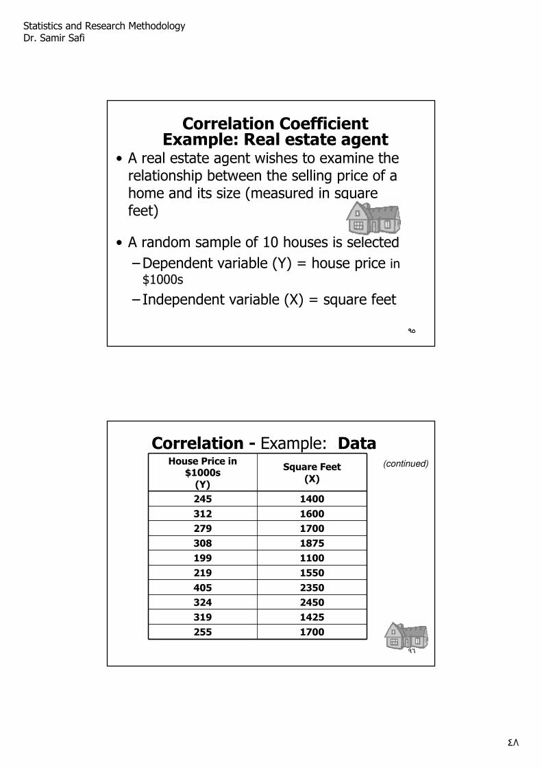
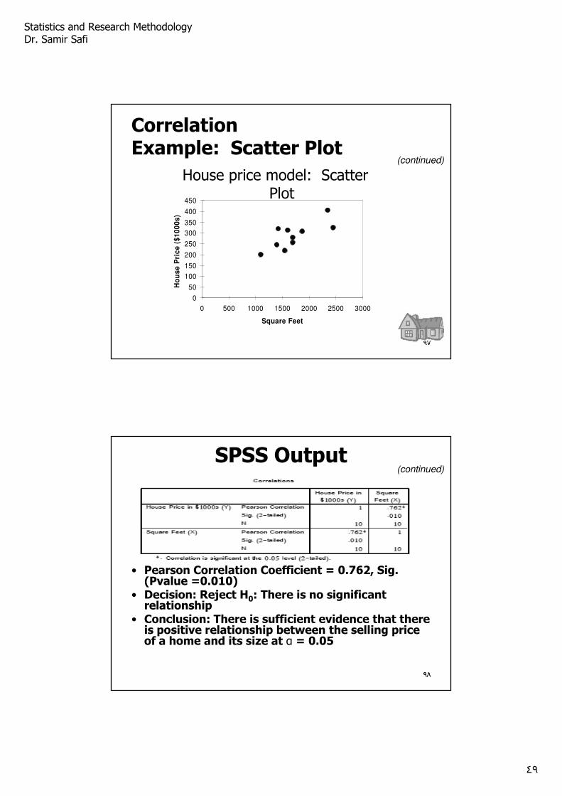
Correlation CoefficientExample: Real estate agent
• A real estate agent wishes to examine the relationship between the selling price of a home and its size (measured in square feet)
• A random sample of 10 houses is selected
– Dependent variable (Y) = house price in
$1000s
– Independent variable (X) = square feet
٩٥
٩٦
Correlation - Example: Data House Price in
$1000s
(Y)
Square Feet
(X)
245 1400
312 1600
279 1700
308 1875
199 1100
219 1550
405 2350
324 2450
319 1425
255 1700
(continued)
٩٦
Statistics and Research Methodology Dr. Samir Safi
٤٩
٩٧
0
50
100
150
200
250
300
350
400
450
0 500 1000 1500 2000 2500 3000
Square Feet
Ho
us
e P
ric
e (
$1
00
0s
)
Correlation Example: Scatter Plot
House price model: Scatter Plot
(continued)
٩٧
٩٨
SPSS Output
• Pearson Correlation Coefficient = 0.762, Sig. (Pvalue =0.010)
• Decision: Reject H0: There is no significant relationship
• Conclusion: There is sufficient evidence that there is positive relationship between the selling price of a home and its size at α = 0.05
(continued)
٩٨
Statistics and Research Methodology Dr. Samir Safi
٥٠
٩٩
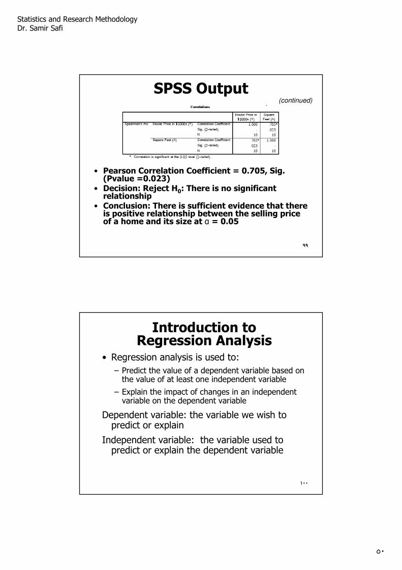
SPSS Output
• Pearson Correlation Coefficient = 0.705, Sig. (Pvalue =0.023)
• Decision: Reject H0: There is no significant relationship
• Conclusion: There is sufficient evidence that there is positive relationship between the selling price of a home and its size at α = 0.05
(continued)
٩٩
١٠٠
Introduction to Regression Analysis
• Regression analysis is used to:
– Predict the value of a dependent variable based on the value of at least one independent variable
– Explain the impact of changes in an independent variable on the dependent variable
Dependent variable: the variable we wish to predict or explain
Independent variable: the variable used to predict or explain the dependent variable
١٠٠
Statistics and Research Methodology Dr. Samir Safi
٥١
١٠١
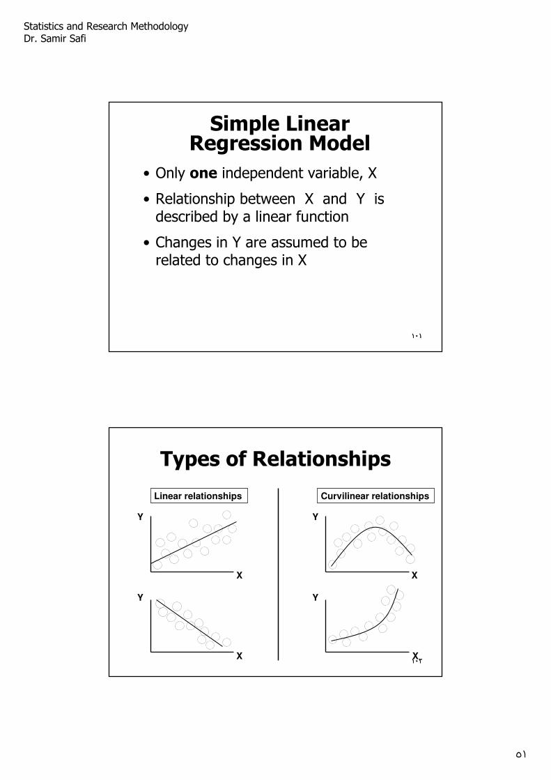
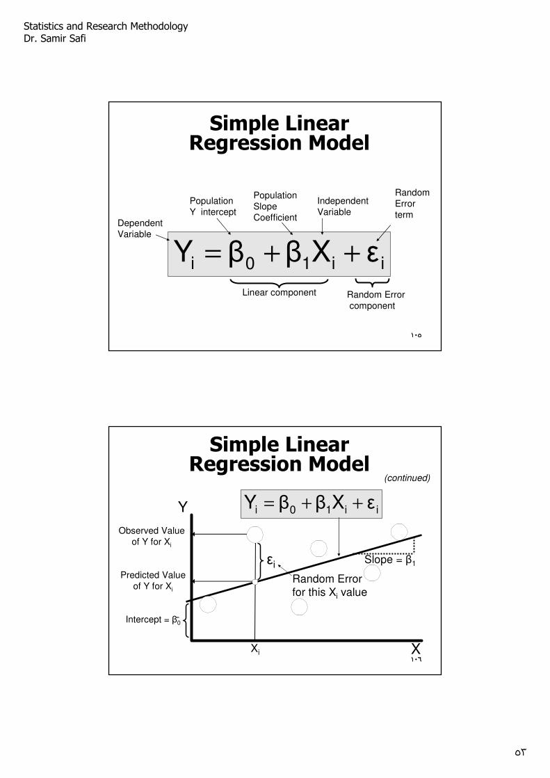
Simple Linear Regression Model
• Only one independent variable, X
• Relationship between X and Y is described by a linear function
• Changes in Y are assumed to be related to changes in X
١٠١
١٠٢
Types of Relationships
Y
X
Y
X
Y
Y
X
X
Linear relationships Curvilinear relationships
١٠٢
Statistics and Research Methodology Dr. Samir Safi
٥٢
١٠٣
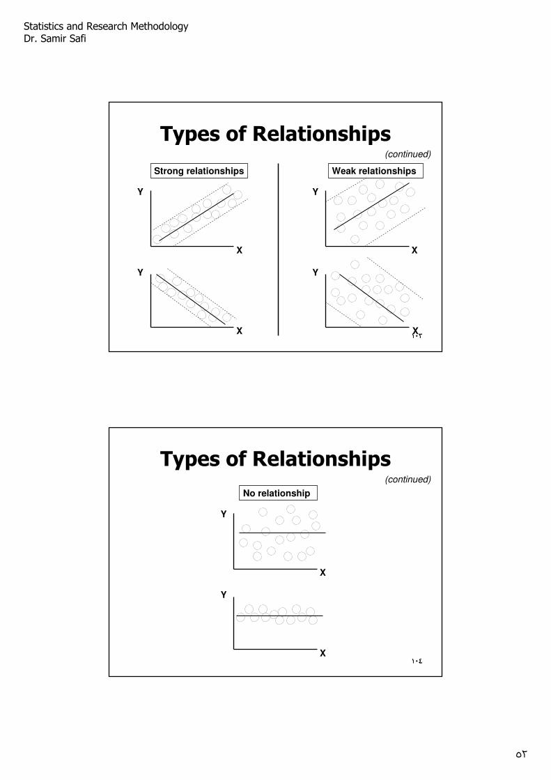
Types of Relationships
Y
X
Y
X
Y
Y
X
X
Strong relationships Weak relationships
(continued)
١٠٣
١٠٤
Types of Relationships
Y
X
Y
X
No relationship
(continued)
١٠٤
Statistics and Research Methodology Dr. Samir Safi
٥٣
١٠٥
ii10i εXββY ++=
Linear component
Simple Linear Regression Model
Population Y intercept
Population SlopeCoefficient
Random Error term
Dependent Variable
Independent Variable
Random Errorcomponent
١٠٥
١٠٦
(continued)
Random Error for this Xi value
Y
X
Observed Value of Y for Xi
Predicted Value of Y for Xi
ii10i εXββY ++=
Xi
Slope = β1
Intercept = β0
εi
Simple Linear Regression Model
١٠٦
Statistics and Research Methodology Dr. Samir Safi
٥٤
١٠٧
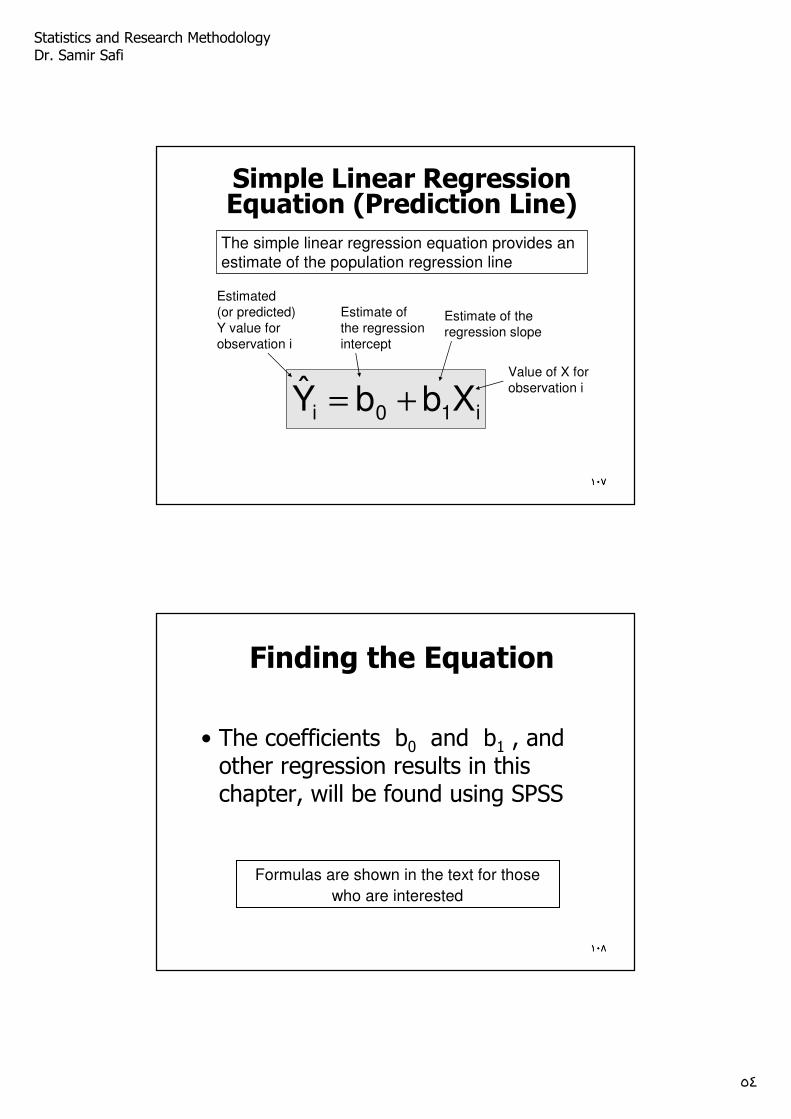
i10i XbbY +=
The simple linear regression equation provides an estimate of the population regression line
Simple Linear Regression Equation (Prediction Line)
Estimate of the regression intercept
Estimate of the regression slope
Estimated (or predicted) Y value for observation i
Value of X for observation i
١٠٧
١٠٨
Finding the Equation
• The coefficients b0 and b1 , and other regression results in this chapter, will be found using SPSS
Formulas are shown in the text for those
who are interested
١٠٨
Statistics and Research Methodology Dr. Samir Safi
٥٥
١٠٩
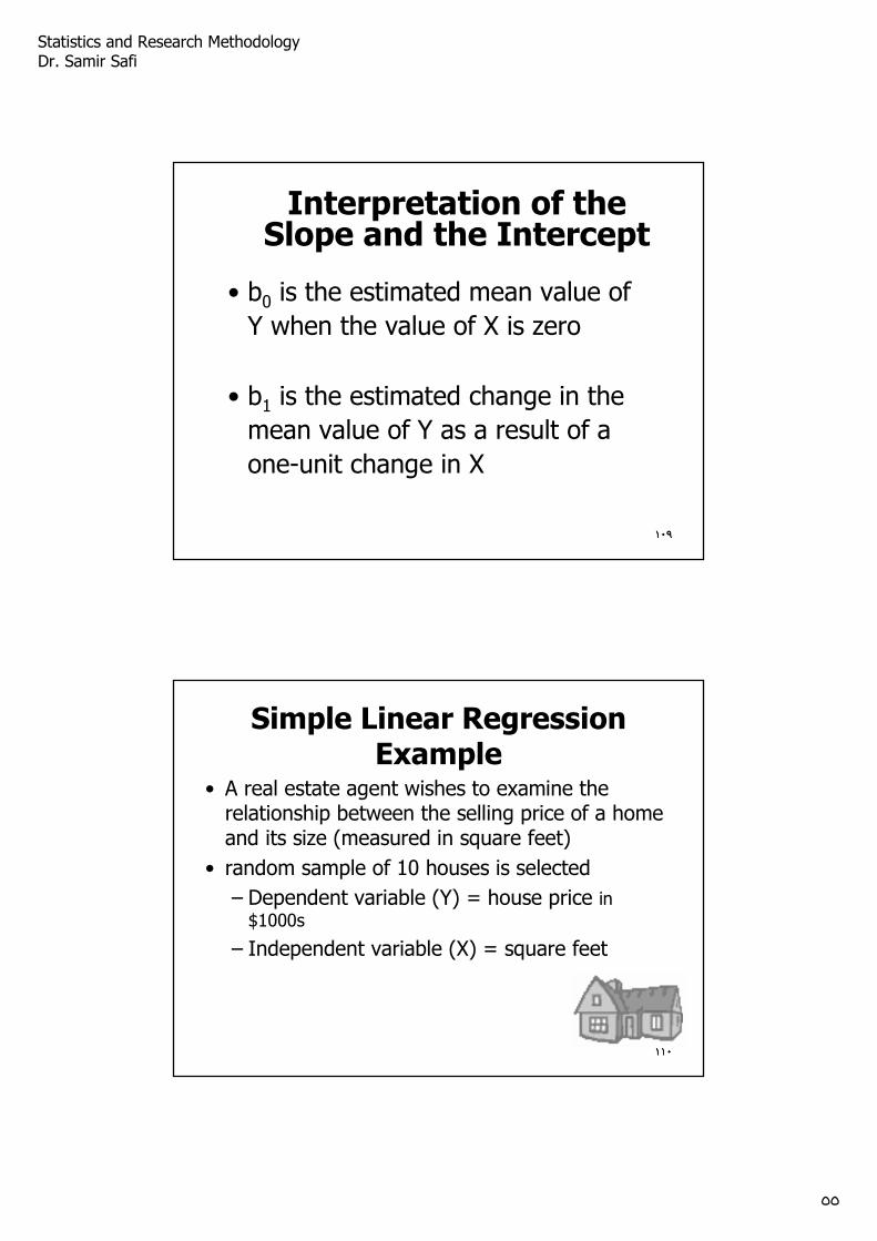
• b0 is the estimated mean value of
Y when the value of X is zero
• b1 is the estimated change in the
mean value of Y as a result of a
one-unit change in X
Interpretation of the Slope and the Intercept
١٠٩
١١٠
Simple Linear Regression Example
• A real estate agent wishes to examine the relationship between the selling price of a home and its size (measured in square feet)
• random sample of 10 houses is selected
– Dependent variable (Y) = house price in
$1000s
– Independent variable (X) = square feet
١١٠
Statistics and Research Methodology Dr. Samir Safi
٥٦
١١١
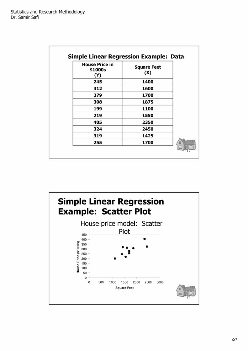
Simple Linear Regression Example: Data
House Price in $1000s
(Y)
Square Feet
(X)
245 1400
312 1600
279 1700
308 1875
199 1100
219 1550
405 2350
324 2450
319 1425
255 1700
١١١
١١٢
0
50
100
150
200
250
300
350
400
450
0 500 1000 1500 2000 2500 3000
Square Feet
Ho
us
e P
ric
e (
$1
00
0s
)
Simple Linear Regression Example: Scatter Plot
House price model: Scatter Plot
١١٢
Statistics and Research Methodology Dr. Samir Safi
٥٧
١١٣
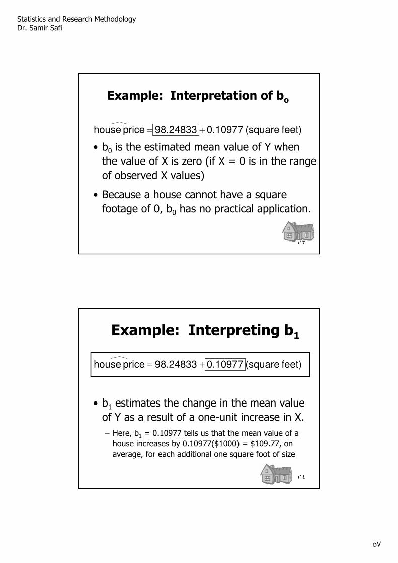
Example: Interpretation of bo
• b0 is the estimated mean value of Y when
the value of X is zero (if X = 0 is in the range
of observed X values)
• Because a house cannot have a square
footage of 0, b0 has no practical application.
feet) (square 0.10977 98.24833 price house +=
١١٣
١١٤
Example: Interpreting b1
• b1 estimates the change in the mean value
of Y as a result of a one-unit increase in X.
– Here, b1 = 0.10977 tells us that the mean value of a
house increases by 0.10977($1000) = $109.77, on
average, for each additional one square foot of size
feet) (square 0.10977 98.24833 price house +=
١١٤
Statistics and Research Methodology Dr. Samir Safi
٥٨
١١٥
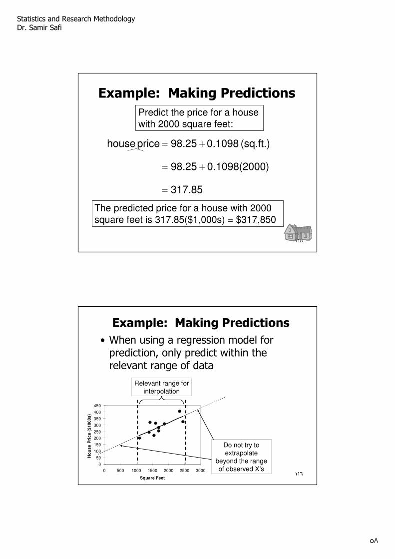
317.85
0)0.1098(200 98.25
(sq.ft.) 0.1098 98.25 price house
=
+=
+=
Predict the price for a house with 2000 square feet:
The predicted price for a house with 2000 square feet is 317.85($1,000s) = $317,850
Example: Making Predictions
١١٥
١١٦
0
50
100
150
200
250
300
350
400
450
0 500 1000 1500 2000 2500 3000
Square Feet
Ho
us
e P
ric
e (
$1
00
0s
)
Example: Making Predictions
• When using a regression model for prediction, only predict within the relevant range of data
Relevant range for interpolation
Do not try to extrapolate
beyond the range of observed X’s
١١٦
Statistics and Research Methodology Dr. Samir Safi
٥٩
١١٧
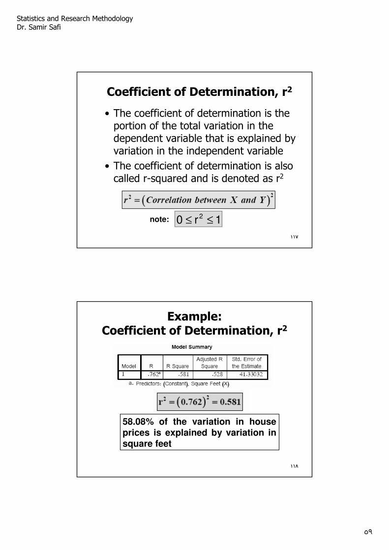
• The coefficient of determination is the portion of the total variation in the dependent variable that is explained by variation in the independent variable
• The coefficient of determination is also called r-squared and is denoted as r2
Coefficient of Determination, r2
1r0 2 ≤≤note:
١١٧
١١٨
Example:Coefficient of Determination, r2
58.08% of the variation in house prices is explained by variation in square feet
١١٨
Statistics and Research Methodology Dr. Samir Safi
٦٠
١١٩
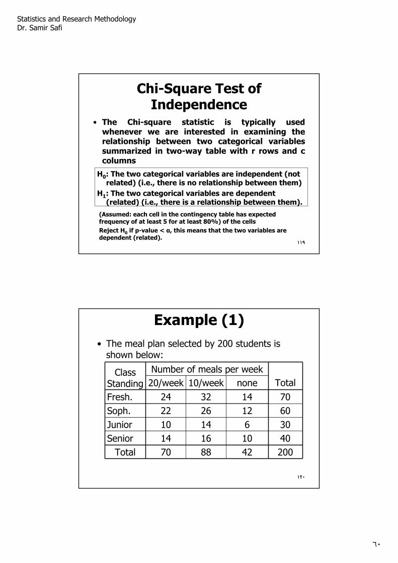
Chi-Square Test of Independence
• The Chi-square statistic is typically used whenever we are interested in examining the relationship between two categorical variables summarized in two-way table with r rows and c columns
H0: The two categorical variables are independent (not related) (i.e., there is no relationship between them)
H1: The two categorical variables are dependent (related) (i.e., there is a relationship between them).
(Assumed: each cell in the contingency table has expected frequency of at least 5 for at least 80%) of the cells
Reject H0 if p-value < α, this means that the two variables are dependent (related).
١١٩
١٢٠
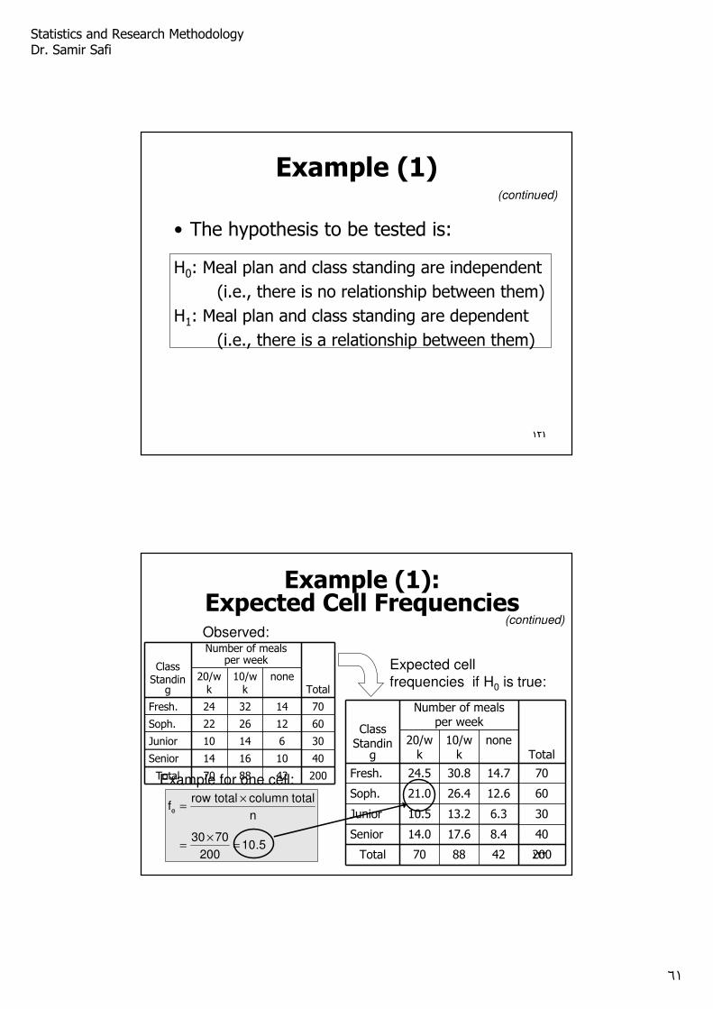
Example (1)
• The meal plan selected by 200 students is shown below:
ClassStanding
Number of meals per week
Total20/week 10/week none
Fresh. 24 32 14 70
Soph. 22 26 12 60
Junior 10 14 6 30
Senior 14 16 10 40
Total 70 88 42 200
١٢٠
Statistics and Research Methodology Dr. Samir Safi
٦١
١٢١
Example (1)
• The hypothesis to be tested is:
(continued)
H0: Meal plan and class standing are independent
(i.e., there is no relationship between them)
H1: Meal plan and class standing are dependent
(i.e., there is a relationship between them)
١٢١
١٢٢
ClassStandin
g
Number of meals per week
Total20/w
k10/w
knone
Fresh. 24 32 14 70
Soph. 22 26 12 60
Junior 10 14 6 30
Senior 14 16 10 40
Total 70 88 42 200
ClassStandin
g
Number of meals per week
Total20/w
k10/w
knone
Fresh. 24.5 30.8 14.7 70
Soph. 21.0 26.4 12.6 60
Junior 10.5 13.2 6.3 30
Senior 14.0 17.6 8.4 40
Total 70 88 42 200
Observed:
Expected cell frequencies if H0 is true:
5.10200
7030
n
total columntotalrow fe
=×
=
×=
Example for one cell:
Example (1): Expected Cell Frequencies
(continued)
١٢٢
Statistics and Research Methodology Dr. Samir Safi
٦٢
١٢٣
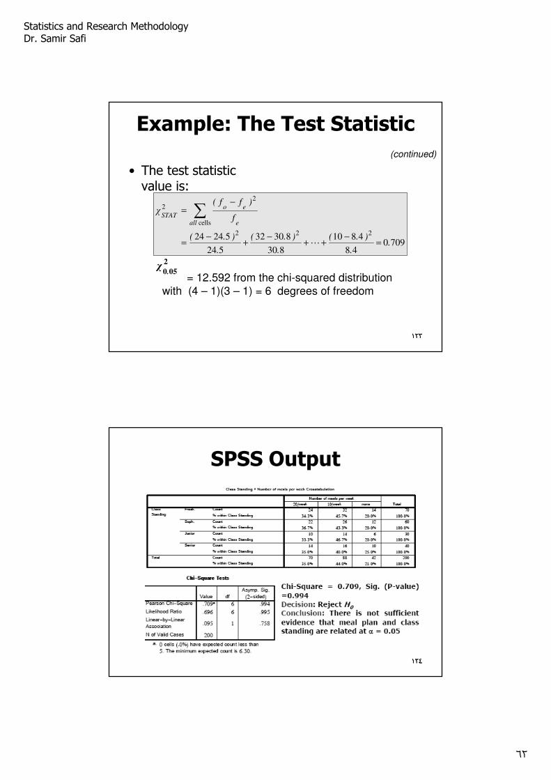
Example: The Test Statistic
• The test statistic value is:
709048
4810
830
83032
524
52424222
cells
2
2
..
).(
.
).(
.
).(
f
)ff(χ
all e
eo
STAT
=−
++−
+−
=
−= ∑
⋯
(continued)
= 12.592 from the chi-squared distribution with (4 – 1)(3 – 1) = 6 degrees of freedom
2
050.χ
١٢٣
١٢٤
SPSS Output
١٢٤
Statistics and Research Methodology Dr. Samir Safi
٦٣
١٢٥
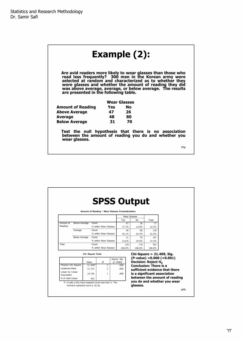
Example (2):
Are avid readers more likely to wear glasses than those who read less frequently? 300 men in the Korean army were selected at random and characterized as to whether they wore glasses and whether the amount of reading they did was above average, average, or below average. The results are presented in the following table.
Wear GlassesAmount of Reading Yes NoAbove Average 47 26Average 48 80Below Average 31 70
Test the null hypothesis that there is no association between the amount of reading you do and whether you wear glasses.
١٢٥
١٢٦١٢٦
SPSS OutputAmount of Reading * Wear Glasses Crosstabulation
47 26 73
37.3% 14.8% 24.2%
48 80 128
38.1% 45.5% 42.4%
31 70 101
24.6% 39.8% 33.4%
126 176 302
100.0% 100.0% 100.0%
Count
% within Wear Glasses
Count
% within Wear Glasses
Count
% within Wear Glasses
Count
% within Wear Glasses
Above Average
Average
Below Average
Amount ofReading
Total
Yes No
Wear Glasses
Total
Chi-Square Tests
21.409a 2 .000
21.354 2 .000
18.326 1 .000
302
Pearson Chi-Square
Likelihood Ratio
Linear-by-LinearAssociation
N of Valid Cases
Value dfAsymp. Sig.(2-sided)
0 cells (.0%) have expected count less than 5. Theminimum expected count is 30.46.
a.
Chi-Square = 21.409, Sig.(P-value) =0.000 (<0.001)Decision: Reject H0
Conclusion: There is asufficient evidence that thereis a significant associationbetween the amount of readingyou do and whether you wearglasses.
١٢٦