1

Spring 2014

Editorial

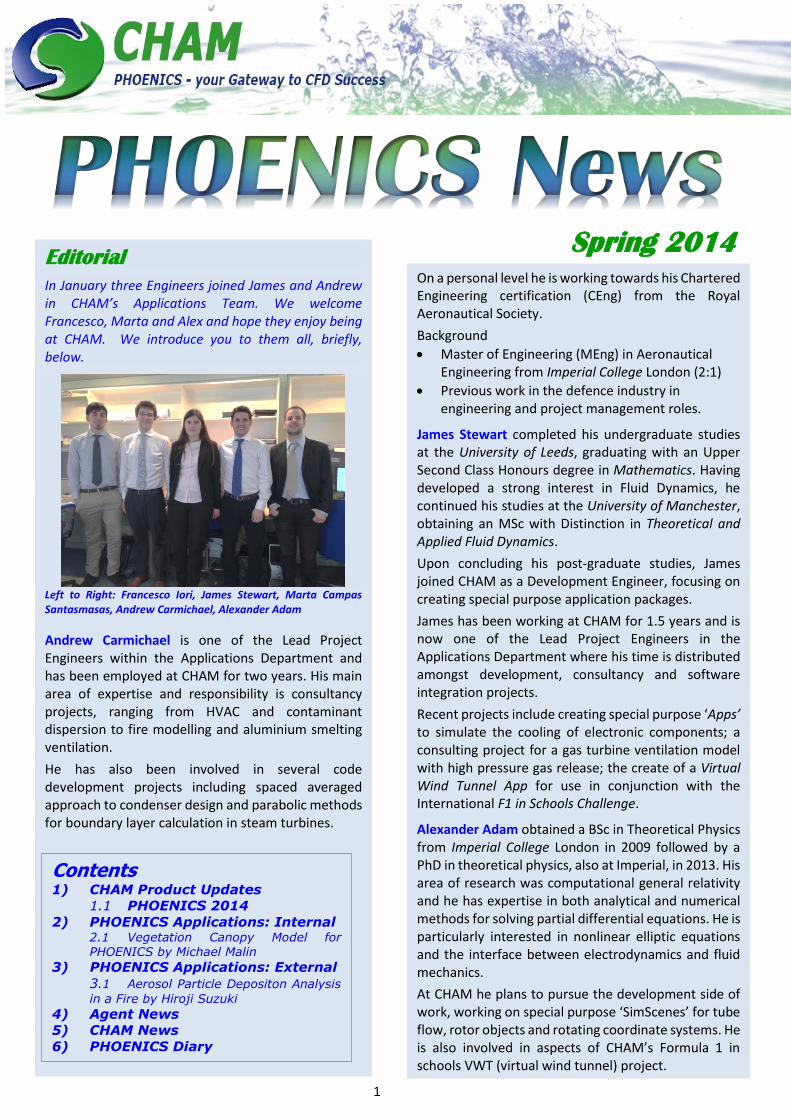
In January three Engineers joined James and Andrew in CHAM’s Applications Team. We welcome Francesco, Marta and Alex and hope they enjoy being at CHAM. We introduce you to them all, briefly, below.

Left to Right: Francesco Iori, James Stewart, Marta Campas Santasmasas, Andrew Carmichael, Alexander Adam

Andrew Carmichael is one of the Lead Project Engineers within the Applications Department and has been employed at CHAM for two years. His main area of expertise and responsibility is consultancy projects, ranging from HVAC and contaminant dispersion to fire modelling and aluminium smelting ventilation.

He has also been involved in several code development projects including spaced averaged approach to condenser design and parabolic methods for boundary layer calculation in steam turbines.

On a personal level he is working towards his Chartered Engineering certification (CEng) from the Royal Aeronautical Society.

Background

Master of Engineering (MEng) in Aeronautical Engineering from Imperial College London (2:1)

Previous work in the defence industry in engineering and project management roles.

James Stewart completed his undergraduate studies at the University of Leeds, graduating with an Upper Second Class Honours degree in Mathematics. Having developed a strong interest in Fluid Dynamics, he continued his studies at the University of Manchester, obtaining an MSc with Distinction in Theoretical and Applied Fluid Dynamics.

Upon concluding his post-graduate studies, James joined CHAM as a Development Engineer, focusing on creating special purpose application packages.

James has been working at CHAM for 1.5 years and is now one of the Lead Project Engineers in the Applications Department where his time is distributed amongst development, consultancy and software integration projects.

Recent projects include creating special purpose ‘Apps’ to simulate the cooling of electronic components; a consulting project for a gas turbine ventilation model with high pressure gas release; the create of a Virtual Wind Tunnel App for use in conjunction with the International F1 in Schools Challenge.

Alexander Adam obtained a BSc in Theoretical Physics from Imperial College London in 2009 followed by a PhD in theoretical physics, also at Imperial, in 2013. His area of research was computational general relativity and he has expertise in both analytical and numerical methods for solving partial differential equations. He is particularly interested in nonlinear elliptic equations and the interface between electrodynamics and fluid mechanics.

At CHAM he plans to pursue the development side of work, working on special purpose ‘SimScenes’ for tube flow, rotor objects and rotating coordinate systems. He is also involved in aspects of CHAM’s Formula 1 in schools VWT (virtual wind tunnel) project.

Contents 1) CHAM Product Updates

1.1 PHOENICS 2014

2) PHOENICS Applications: Internal 2.1 Vegetation Canopy Model for

PHOENICS by Michael Malin

3) PHOENICS Applications: External

3.1 Aerosol Particle Depositon Analysis

in a Fire by Hiroji Suzuki

4) Agent News

5) CHAM News

6) PHOENICS Diary

2

Marta Camps Santasmasas obtained a BSc in Aeronautical Engineering at the Universitat Politecnica de Catalunya (UPC) in Castelldefels, Spain in 2006.

This course awakened her interest in fluid mechanics and she decided to study it in greater depth through an MSc in Computational and Applied Physics at the Universitat Politecnica de Catalunya (UPC) and Universitat de Barcelona (UB) in Barcelona, Spain (2007-2010).

She specialised in Computational Fluid Mechanics and in 2009 she was offered a position in Normawind, a renewable energy consultancy. Her main responsibilities included the wind resource and site assessment through CFD for wind farm projectsShe was also the main researcher for the R+D project to incorporate CFD modelling as a new service to assess the wind characteristics in a wind farm site. Marta is currently developing the Wind Tunnel SimScene, beginning with the city scape version.

Francesco Iori obtained a BSc and an MSc in Medical Engineering at the University of Rome, “Tor Vergata”, respectively in 2011 and 2013. During the last year of his MSc, he became interested in the study of biological fluid dynamics and in particular of CFD methods applied to the simulation of blood flows.

In November 2012 he took part in the students’ exchange programme “Erasmus Placement”, and spent one year at the Department of Bioengineering of Imperial College, London, where he also completed his Master’s Thesis. During this period, he investigated the effect of arterial curvature in end-to-side arterio-venous fistulae, on haemodynamic factors and blood-to-wall oxygen transport and their correlation with the development of vascular pathology.

At CHAM, Francesco is currently working on the development of a SimScene, which will allow users to simulate steady and transient flows, in geometrically realistic shell and tube heat exchangers.

1. PHOENICS Product Updates

1.1 PHOENICS 2014

PHOENICS 2014 is currently in the last stages of development and testing within CHAM. The major feature of PH-2014 will be its new S-PARSOL feature for handling very thin objects that can cut cells more than once. This feature will be described fully in the Summer Issue whilst, in this article, other improvements are outlined.

In PHOENICS/Flair Specification of pollutants - up to 5 pollutants can

be defined simply through its menu.

Emissivity - improved function of smoke and temperature.

Wet bulb, Dew point, Wet Bulb Globe temperatures have been made available.

Prototype ‘Heatisle’ module has been extended.

New foliage model – see article in Section 2, below.

In PHOENICS/CVD DC potential calculation introduced.

In General Datmaker / SIMLAB Composer CAD import and

conversion utility.

Ability to dump PNG files instead of GIF. Choice of grid plane display X,Y,Z or Auto.

In the VR-Editor Preservation of CAD file extensions used in Q1.

Preservation of the Shapemaker.geo extension in Q1 and allow further adjustments.

Ability to drag and drop CAD files into VRE window.

Disallow negative MAXINC.

Copy as array now has offsets in the other two directions to create diagonal copies.

Option to move probe to centre of current object.

Save as case moves transient files into case folder instead of copying them.

Save as case does not create new Q1 before saving if RESULT is newer than Q1 to ensure matching files are saved.

For the Viewer Save and read colour palette from macro.

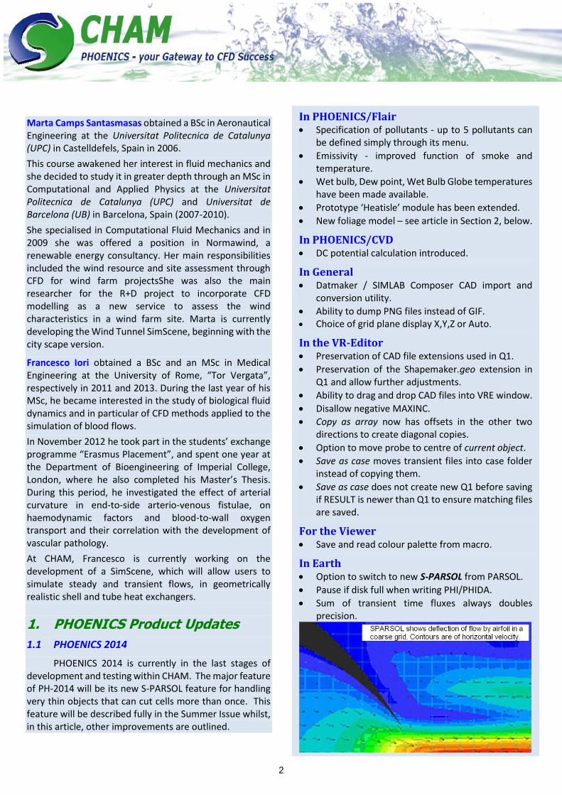
In Earth Option to switch to new S-PARSOL from PARSOL.

Pause if disk full when writing PHI/PHIDA.

Sum of transient time fluxes always doubles precision.

3

2. PHOENICS Applications: Internal Users

2.1 Vegetation Canopy Model for PHOENICS by Michael R Malin (extended from Spring News)

Introduction Interest has been expressed by various companies in using PHOENICS to simulate interaction between the wind and forested areas, and other types of tree or plant canopy, including urban plantings of avenues or tree clumps. PHOENICS has been equipped, therefore, with a vegetation canopy model to simulate effects of vegetation by introducing flow resistance terms in the momentum equations, and turbulence production and destruction terms in turbulence transport equations.

From an aerodynamic perspective, the main impact of vegetation on the environment is the reduction in air velocity due to drag forces, and the additional turbulence levels produced by the canopy elements. In PHOENICS these effects are represented by a porous-media approach based on superficial velocities where momentum sinks and turbulence sources are applied to a block of cells chosen to represent the tree canopy.

Flow resistance due to turbulent flow through the plant canopy is represented by a momentum sink term dependent on the superficial velocity vector, the drag coefficient, and the leaf area density (LAD) perpendicular to the flow direction. The default PHOENICS model uses a constant effective drag coefficient Cd and a constant effective LAD, although provision is made for the user to specify a vertical distribution of the LAD. The canopy model also introduces additional source and sink terms into the transport equations for the turbulent kinetic energy k and its dissipation rate ɛ. These terms account for turbulence production and accelerated turbulence dissipation within the canopy.

Implementation & User Input The canopy model has been implemented into the PHOENICS-VR Environment (VRE) by means of the FOLIAGE object, which allows the user to specify the foliage location and volume, and then set the input parameters needed in the model. The object also produces the INFORM commands needed to implement the momentum sink and turbulence source/sink terms into the finite-volume equations in linearised form.

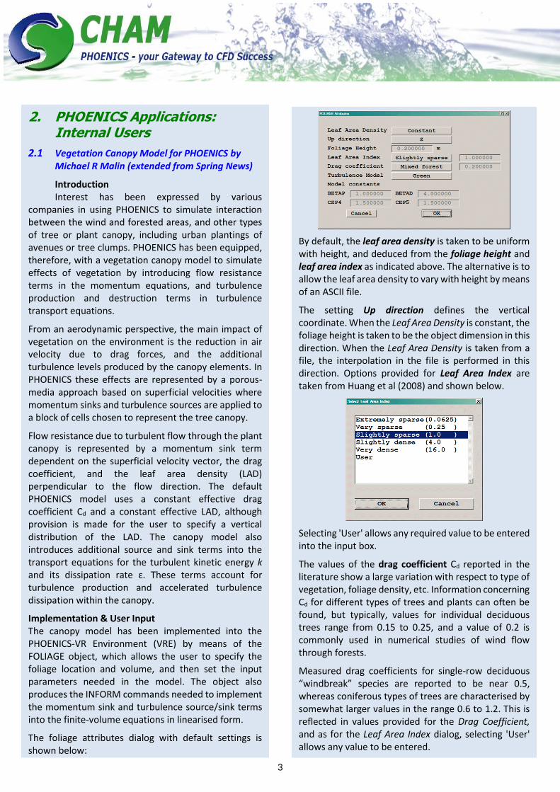
The foliage attributes dialog with default settings is shown below:

By default, the leaf area density is taken to be uniform with height, and deduced from the foliage height and leaf area index as indicated above. The alternative is to allow the leaf area density to vary with height by means of an ASCII file.

The setting Up direction defines the vertical coordinate. When the Leaf Area Density is constant, the foliage height is taken to be the object dimension in this direction. When the Leaf Area Density is taken from a file, the interpolation in the file is performed in this direction. Options provided for Leaf Area Index are taken from Huang et al (2008) and shown below.

Selecting 'User' allows any required value to be entered into the input box.

The values of the drag coefficient Cd reported in the literature show a large variation with respect to type of vegetation, foliage density, etc. Information concerning Cd for different types of trees and plants can often be found, but typically, values for individual deciduous trees range from 0.15 to 0.25, and a value of 0.2 is commonly used in numerical studies of wind flow through forests.

Measured drag coefficients for single-row deciduous “windbreak” species are reported to be near 0.5, whereas coniferous types of trees are characterised by somewhat larger values in the range 0.6 to 1.2. This is reflected in values provided for the Drag Coefficient, and as for the Leaf Area Index dialog, selecting 'User' allows any value to be entered.

4

Turbulent interaction between the airflow and the vegetation is simulated by including additional source and sink terms in each of the transport equations for k and ε. This involves four empirical constants, and there is little consensus in the literature about their recommended values which reflects the fact that different values are needed to match different sets of measured data. The default values used by the FOLIAGE object are those of Green (1992), but provision is made via Turbulence Model for the user to select from five other sets of turbulence-model constants, as proposed by authors listed in the "Select Turbulence modification" drop-down menu.

Selecting 'None' switches off plant-canopy terms in the turbulence transport equations. Selecting 'User' allows any desired values to be input for the empirical constants.

Application to the Harwood spruce forest There have been only a small number of experimental studies of wind flow through trees, and even then the number of data points are limited, and the accuracy of the measurements in such difficult conditions remains questionable. Here, two-dimensional simulations are made of the transition from open land to forest by replicating the field study of the Harwood spruce forest in Northumberland, as documented by

Dalpe & Masson (2007) and Krzikalla (2005). The forest consists of a uniform plantation of Sitka spruce with the following characteristics: forest tree height, h=7.5m; leaf area index, LAI = 2.15; and an effective drag coefficient, cd = 0.2.

The wind conditions upstream of the forest are represented by a logarithmic velocity profile with a reference velocity of 6.28m/s at a height of 15m, and an open-land roughness height z0=0.0028m. This means that the wind friction velocity u* = 0.3m/s.

The spruce canopies are modelled by assuming a constant LAD calculated from equation as LAI/h =0.287 m2/m3. The forest is 20h long, and the solution domain is 80h long by 20h high. The wind inlet boundary is located 20h upstream of the forest's leading edge, and a fixed-pressure boundary is located 20h behind the lee of the forest.

A non-uniform mesh is used with 60 cells in the vertical direction (z) and 210 cells in the axial direction (x). The forest occupies 20 by 100 cells in the vertical and axial directions, respectively. A fixed-pressure boundary condition is applied at the top of the solution domain.

Figure 1 (below and next page) presents contour plots showing the transition from open land to forest in terms of velocity vectors, pressure and turbulent kinetic energy. The simulations are made using the turbulence-model coefficients of Green (1992), and in the figure the pressure and turbulence energy are normalised with the friction velocity of the approach flow.

5

Figure 1: Harwood forest: Computed distributions of velocity, pressure and turbulent kinetic energy normalised with the friction velocity of the approach flow.

Figure 1 shows that wind flow enters the forest, where it experiences drag forces and decelerates, entailing a strong pressure gradient in the flow direction. The mean flow is deflected upwards, and there is significant turbulence generation at the canopy-air interface due to mean shear, and the turbulence diminishes markedly with depth into the canopy.

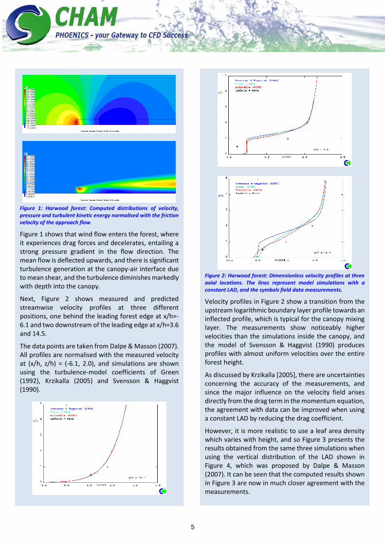
Next, Figure 2 shows measured and predicted streamwise velocity profiles at three different positions, one behind the leading forest edge at x/h=-6.1 and two downstream of the leading edge at x/h=3.6 and 14.5.

The data points are taken from Dalpe & Masson (2007). All profiles are normalised with the measured velocity at (x/h, z/h) = (-6.1, 2.0), and simulations are shown using the turbulence-model coefficients of Green (1992), Krzikalla (2005) and Svensson & Haggvist (1990).

Figure 2: Harwood forest: Dimensionless velocity profiles at three axial locations. The lines represent model simulations with a constant LAD, and the symbols field data measurements.

Velocity profiles in Figure 2 show a transition from the upstream logarithmic boundary layer profile towards an inflected profile, which is typical for the canopy mixing layer. The measurements show noticeably higher velocities than the simulations inside the canopy, and the model of Svensson & Haggvist (1990) produces profiles with almost uniform velocities over the entire forest height.

As discussed by Krzikalla [2005], there are uncertainties concerning the accuracy of the measurements, and since the major influence on the velocity field arises directly from the drag term in the momentum equation, the agreement with data can be improved when using a constant LAD by reducing the drag coefficient.

However, it is more realistic to use a leaf area density which varies with height, and so Figure 3 presents the results obtained from the same three simulations when using the vertical distribution of the LAD shown in Figure 4, which was proposed by Dalpe & Masson (2007). It can be seen that the computed results shown in Figure 3 are now in much closer agreement with the measurements.

6

Figure 3: Harwood forest: Dimensionless velocity profiles at three axial locations. The lines represent model simulations, and the symbols field data measurements.

Figure 4: Harwood forest: Vertical distribution of the leaf area density.

Conclusions A vegetation canopy model has been implemented into the PHOENICS code using a porous-media approach and a modified k-ɛ turbulence model. The main parameters describing the momentum losses in the canopy are the drag coefficient and the leaf area density perpendicular to the flow direction.

The default in PHOENICS is to use a constant leaf-area density, but provision is made for the user to specify a variation with height.

Further validation of the model is needed against measured data, but the results presented here for the Harwood forest are encouraging in terms of the agreement obtained between the predicted and measured wind velocities. References Dalpe, B. & Masson, C. “Recommended practices when analysing wind flow near a forest edge with WASP”, European Wind Energy Conference, Milan, Italy (2007).

Green, R.S., "Modelling turbulent air flow in a stand of widely-spaced trees", PHOENICS Journal, 5:294–312, (1992).

Huang, J., Cassiani, M. & Albertson, J., "The effects of vegetation density on turbulent structures within canopy sublayer", AMS, Paper 2.2, (2008).

Irvine, M.R., Gardiner, B.A., & Hill, M.K., "The evolution of turbulence across a forest edge. Boundary-Layer Meteorology", 84:467–496, (1997).

Krzikalla, F., "Numerical investigation of the interaction between wind and forest under heterogeneous conditions", PhD Thesis, Institute for Hydromechanics, University of Karlsruhe, Germany, (2005).

Liu, J., Chen, J.M., Black, T.A. & Novak, M.D., "k-ɛ modelling of turbulent air flow downwind of a model forest edge". Boundary-Layer Meteorology, 72:21–44, (1998).

Lopes da Costa, J. C. "Atmospheric Flow over Forested and Non-forested Complex Terrain", PhD thesis, University of Porto, (2007).

Sanz, C. "A note on k-ɛ modelling on a vegetation canopy", Boundary-Layer Meteorology", 108:191–197, (2003).

Svensson, U. & Haggkvist, K., "A two-equation turbulence model for canopy flows", Journal of Wind Engineering and Industrial Aerodynamics, 35:201–211, (1990).

7

3. PHOENICS Applications: External Users

3.1 Aerosol Particle Deposition Analysis in a Fire by Hiroji Suzuki

1. Introduction Aerosol particles generated in a fire at an

industrial site include a harmful substance. It is important to compute the particle distribution to protect the human body from harm.

So the aerosol particle deposition model is implemented in PHOENICS 2010 via the User’s subroutine (Ground) to simulate the behavior of the aerosol particles (smoke) generated in a fire. The confirmation calculation is done by 3D rectangular model (Fig.1) with buoyancy considered. This is a transient calculation to 1000 sec.

Fig.1 Computational Model Unit[m]

2. Governing Equation

The governing equation for each dependent variable is the following.

Sgradudivt

(1)

where

: dependent variable

: density of fluid

u

: velocity vector

: exchange coefficient,

t

t

l

l

: kinematic viscosity : Prandtl number

S : source term for the each

t : time

Dependent Variable S

1 (mass) 0

u

=(U,V,W) (momentum) P

T (temperature) Q

Ci (aerosol particle concentration)

Si

Table 1 P : pressure Q : heat source Si : deposition rate

2.1 Terminal Settling Velocity for Aerosol Particle

The terminal settling velocity of aerosol particle i

iw is computed by the following terminal settling

velocity equation of Stokes.

18

2

, ifip

i

dgw

(2)

where f : density of fluid

ip, : density of particle i

g : gravity acceleration

id : diameter of particle i

: viscosity of fluid

When iC , gravitational direction velocity

component : iW is

ii wWW (3)

2.2 Deposition Flux of Aerosol Particles on the Wall

1) Laminar Diffusion Deposition Flux

z

nDll (4)

Where

l : deposition flux of laminar diffusion for the wall

lD : diffusion coefficient of Stokes-Einstein

n : concentration of aerosol particles

z : normal direction for the wall

s

8

2) Turbulent Diffusion Deposition Flux

z

nDtt (5)

where tD : turbulent diffusion coefficient

The following total diffusion deposition flux is drawn by eq. (4) and (5)

z

nDD tldif (6)

where dif : total diffusion deposition flux

3) Thermophoretic Deposition Flux

Thermophoretic velocity: thV is computed by the

following eq.(7).

z

T

KCkkk

KCkk

KCT

AKV

g

ntaag

ntag

nmg

ng

th

22312

13

(7)

Where:

g : kinematic viscosity

A : experimental value of Millikan

nK : Knudsen number

gT : gas temperature

mC : correction coefficient for the temperature

discontinuity

tC : correction coefficient for the momentum

transport effect

: shape factors

gk : thermal conductivity of gas

ak : thermal conductivity of the aerosol particles

Thermophoretic Deposition Flux:th is shown by eq.(8)

nVthth (8)

4) Gravitational Deposition Flux

Gravitational deposition flux is drawn by eq.(2)

nwig (9)

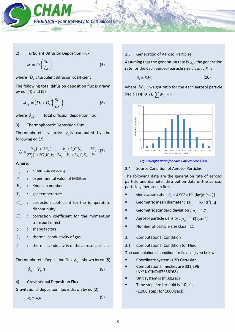
2.3 Generation of Aerosol Particles

Assuming that the generation rate is 0S , the generation

rate for the each aerosol particle size class i : iS is

iti WSS ,0 (10)

where itW , : weight ratio for the each aerosol particle

size class(Fig.2), i

itW 1,

Fig.2 Weight Ratio for each Particle Size Class

2.4 Source Condition of Aerosol Particles

The following data are the generation rate of aerosol particle and diameter distribution data of the aerosol particle generated in fire.

Generation rate : sec)][kg/(m104.903= 3-3

0 S

Geometric mean diameter : [m]104.0= -7

g D

Geometric standard deviation : .71=g

Aerosol particle density : ][kg/m0.1= 3

p

Number of particle size class : 11

3. Computational Condition

3.1 Computational Condition for Fluid

The computational condition for fluid is given below.

Coordinate system is 3D Cartesian

Computational meshes are 331,296 (NX*NY*NZ=87*56*68)

Unit system is (m,kg,sec)

Time step size for fluid is 1.0[sec]

(1,000[step] for 1000[sec])

9

Property of fluid Density : 1.176 [kg/m3](Air) Kinematic viscosity : 1.583E-5[m2/sec] Thermal conductivity : 0.0258[W/(mK)] Specific heat at constant volume : 1007[J/(kgK)]

Boundary condition Inlet : Inlet velocity 2[m/sec] Outlet : gauge pressure 0[Pa] Wall : Non-slip Outside temperature : 30[Deg.C] Heat generation rate in fire region : 4E+6[W/m3]

Turbulence model LVEL model

Buoyancy Boussinesq approximation

Radiation IMMERSOL method Scattering coefficient : 0.8 Absorption coefficient : 0.8

Initial condition Steady state situation with no heat generation

4. Result

The total aerosol particle concentration distribution for all particle size classes at the cross section for the y axis is shown in Fig.3. The time integral value of deposition on each wall is shown in Fig.4. The value of deposition at the center of the top wall is highest, because the highest value of the deposition flux is caused by high total aerosol particle concentration for all size classes (Fig.3) and high fluid temperature (Fig.5).

100[sec]

300[sec] 1000[sec]

Fig.3 Total Aerosol Particle Concentration for All Size Class

100[sec]

300[sec] 500[sec]

700[sec] 1000[sec]

Fig.4 Time Integral Value of Deposition on the wall [kg/m2]

100[sec]

300[sec] 1000[sec]

Fig.5 Temperature[Deg.C]

Fig.6 Velocity Vector[m/sec] (300[sec])

10

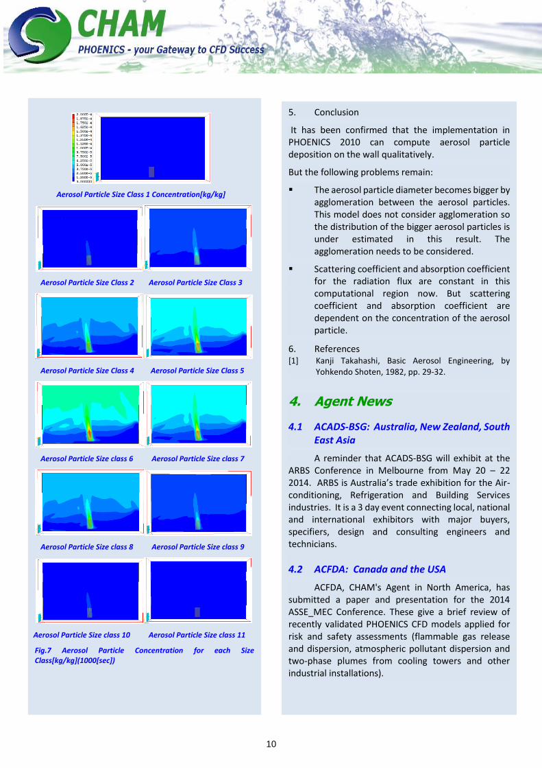
Aerosol Particle Size Class 1 Concentration[kg/kg]

Aerosol Particle Size Class 2 Aerosol Particle Size Class 3

Aerosol Particle Size Class 4 Aerosol Particle Size Class 5

Aerosol Particle Size class 6 Aerosol Particle Size class 7

Aerosol Particle Size class 8 Aerosol Particle Size class 9

Aerosol Particle Size class 10 Aerosol Particle Size class 11

Fig.7 Aerosol Particle Concentration for each Size Class[kg/kg](1000[sec])

5. Conclusion

It has been confirmed that the implementation in PHOENICS 2010 can compute aerosol particle deposition on the wall qualitatively.

But the following problems remain:

The aerosol particle diameter becomes bigger by agglomeration between the aerosol particles. This model does not consider agglomeration so the distribution of the bigger aerosol particles is under estimated in this result. The agglomeration needs to be considered.

Scattering coefficient and absorption coefficient for the radiation flux are constant in this computational region now. But scattering coefficient and absorption coefficient are dependent on the concentration of the aerosol particle.

6. References [1] Kanji Takahashi, Basic Aerosol Engineering, by

Yohkendo Shoten, 1982, pp. 29-32.

4. Agent News

4.1 ACADS-BSG: Australia, New Zealand, South East Asia

A reminder that ACADS-BSG will exhibit at the ARBS Conference in Melbourne from May 20 – 22 2014. ARBS is Australia’s trade exhibition for the Air-conditioning, Refrigeration and Building Services industries. It is a 3 day event connecting local, national and international exhibitors with major buyers, specifiers, design and consulting engineers and technicians.

4.2 ACFDA: Canada and the USA

ACFDA, CHAM's Agent in North America, has submitted a paper and presentation for the 2014 ASSE_MEC Conference. These give a brief review of recently validated PHOENICS CFD models applied for risk and safety assessments (flammable gas release and dispersion, atmospheric pollutant dispersion and two-phase plumes from cooling towers and other industrial installations).

11

These materials show PHOENICS modelling capabilities and underline the beneficial use of CFD in risk and safety analyses. More information on the models and training/consulting options could be obtained by contacting info@acfda.org

The paper, and the presentation, can be accessed via the Agent / Contact page of the CHAM website http://www.cham.co.uk/agents.php.

5) CHAM News

5.1 CHAM London

CHAM wishes all PHOENICS Users an enjoyable and relaxing Easter Holiday period.

We invite all PHOENICS Users and CHAM Agents to submit articles, news items, or general information for inclusion in the PHOENICS Newsletter to cik@cham.co.uk. We would be delighted to hear from you. Please send any submissions in Word format so that they can be tailored to fit the space available. Thank you.

5.2 Visit to Singapore and Hong Kong

Dr David Glynn visited Singapore in late February to train personnel at Jurong Town Corporation, together with members of CHAM’s agency in Singapore, ZEB Technologies.

JTC plays a large part in master planning and urban design; concerned with "infrastructure solutions" throughout Singapore and attendees were members of a working group focussed particularly towards thermal “Urban Heat Island” studies.

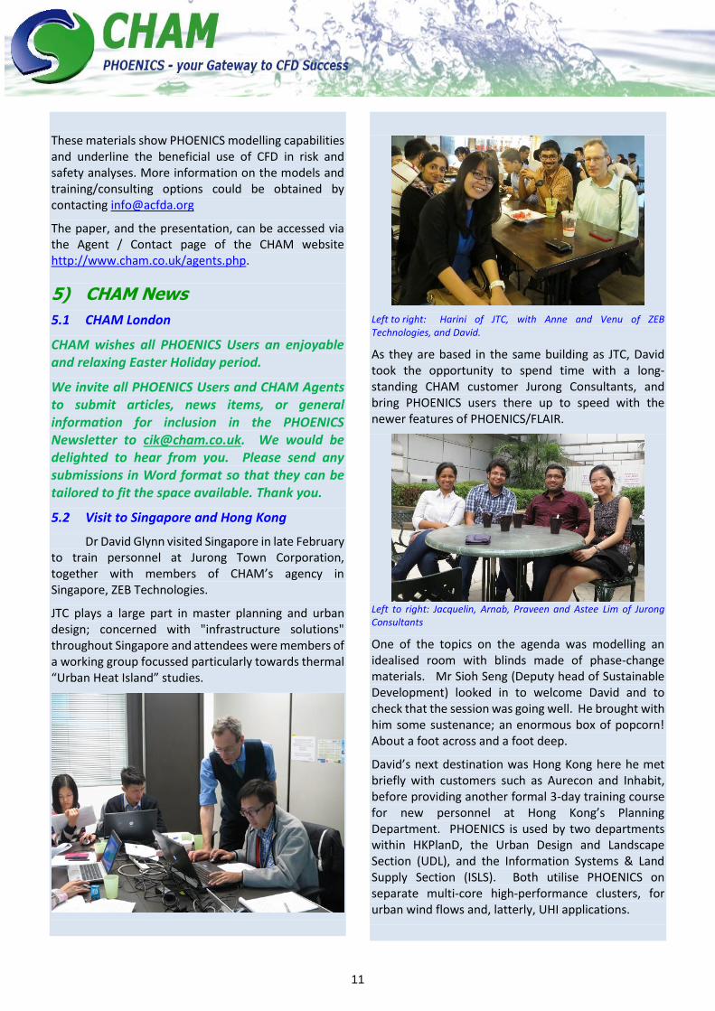
Left to right: Harini of JTC, with Anne and Venu of ZEB Technologies, and David.

As they are based in the same building as JTC, David took the opportunity to spend time with a long-standing CHAM customer Jurong Consultants, and bring PHOENICS users there up to speed with the newer features of PHOENICS/FLAIR.

Left to right: Jacquelin, Arnab, Praveen and Astee Lim of Jurong Consultants

One of the topics on the agenda was modelling an idealised room with blinds made of phase-change materials. Mr Sioh Seng (Deputy head of Sustainable Development) looked in to welcome David and to check that the session was going well. He brought with him some sustenance; an enormous box of popcorn! About a foot across and a foot deep.

David’s next destination was Hong Kong here he met briefly with customers such as Aurecon and Inhabit, before providing another formal 3-day training course for new personnel at Hong Kong’s Planning Department. PHOENICS is used by two departments within HKPlanD, the Urban Design and Landscape Section (UDL), and the Information Systems & Land Supply Section (ISLS). Both utilise PHOENICS on separate multi-core high-performance clusters, for urban wind flows and, latterly, UHI applications.

12

Training group from ISLS, Hong Kong Planning Dept.

CHAM’s Steve Mortimore prepared the ground by installing PHOENICS onto the training computers, as well as updating the main HPC installation.

The final training session was attended by the Senior Town Planner, Mr Ng, who put David on the spot by wanting to see one of HKPlanD’s buildings cases being imported into PHOENICS and then run within a Tutorial Session. Despite being very complex, David managed to import the CAD file, mesh and define the case, and demonstrate a passable flow field within the short time available, and to everyone's satisfaction. The course was very well received, and another such course is envisaged for HK PlanD personnel, later in 2014.

6) PHOENICS Diary

2014 Activity

On going

Shanghai Feiyi will hold PHOENICS training courses in cities including Fuzhou and Nanchang as well as in Shanghai. Please see www.shanghaifeiyi.cn.

On going

C-h-a-m-p-i-o-n, Taiwan provides regular basic and advanced training. See www.c-h-a-m-p-i-o-n.com.tw or contact: sales@c-h-a-m-p-i-o-n.com.tw.

On going

CHAM London holds regular PHOENICS training courses. Please see www.cham.co.uk

On going

Focus Advance Technologies, Malaysia, provides training for beginners, intermediate and advanced CFD users. The training for beginners is usually for first time users with zero background in engineering. Intermediate training is for those with an engineering background who wanted to add new skills. Advanced user training is for those who use CFD regularly but require deeper understanding of the theory behind the CFD software. www.focus-technologies.com.my

On going

ACFDA, Canada, provides multi-level training to ensure that customers become knowledgeable users of CFD models and PHOENICS CFD software. Various training course options are available: 1. Basic 3-day course for new users (includes free 1-

month license & client application work template). 2. Advanced courses featuring specific PHOENICS

features such as modelling multiphase flows, combustion, etc.

3. Customized courses to suit client requirements. Training sessions can be at the Toronto office, on client sites or over the internet. Contact info@acfda.org.

Mar 18 2014

Shanghai Feiyi will hold a basic PHOENICS training course at Zhengzhou University. Please see www.shanghaifeiyi.cn.

Mar 28

Shanghai Feiyi will be exhibiting PHOENICS in Beijing. University. Please see www.shanghaifeiyi.cn.

Apr 2014

Shanghai Feiyi will hold a PHOENICS User training course at Zhejiang University. Please see www.shanghaifeiyi.cn.

Apr 2014

Shanghai Feiyi will hold a PHOENICS USER MEETING in Shanghai. Please see www.shanghaifeiyi.cn

May 2014

ACADS-BSG will exhibit PHOENICS at the ARBS conference in Melbourne Australia. Please see www.ozemail.com.au/~acadsbsg.

May 20-22 2014

Shanghai Feiyi will hold a basic PHOENICS training course at Jiangxi Ganzhou. Please see www.shanghaifeiyi.cn.