Psychology Department

SPSS Version 17 A Beginner’s Guide to SPSS for Windows: Entering and Analysing Questionnaire data Semester 2, 2009-2010

1

1. Introduction This booklet is not intended as a complete guide to SPSS, questionnaire design or data analysis. It is simply meant to help you to become familiar with the use of SPSS in your practical work as a means to understanding and analysing data.

The booklet is divided into several sections, which can be referred to separately, or on the other hand you may like to follow it step by step using the examples to code, input and analyse your own questionnaire data.

A sample questionnaire is used throughout to demonstrate how to apply the instructions. It is based on a survey of childhood experiences of independence and attitudes to accompanying children to school. A small data file has been created, containing 54 cases, designed to illustrate some of the basic features of SPSS covered in this guide. You can enter the data listed in the Appendix using the Data window. This will allow you to check the results of your SPSS analysis against the examples in this guide.

This booklet refers to SPSS version 17 which is installed in C224. If you use other SPSS versions then most of the commands will be the same and you should be able to move your data files between the different versions, but you will not be able to open output files with earlier SPSS versions. If you need to open output files created by earlier versions of SPSS, you will need to use a separate program called SPSS SmartViewer.

The data file is available on the Brookes network in two forms:

U:\data\SOCSCI\spssraw.sav contains the raw data as listed in the appendix

U:\data\SOCSCI\spssvalues.sav contains the same data but includes value labels and

some new recoded variables.

This booklet is distributed free to Undergraduate Psychology students in module U24103 and to students in module U24137 who have not previously taken U24103. Please keep it safe, since it will be useful to you throughout your degree.

Replacements may be charged at £5 per copy.

Postgraduate Psychology students are also entitled to one free copy.

Copyright © Psychology Department, Oxford Brookes University, 1996-2010.

Last Revised – January, 2010.

2

Contents

1.  Introduction 1 

2.  Coding and naming variables 5 Travel Questionnaire 6 

3.  A brief introduction to SPSS for Windows 8 3.1  Getting started in SPSS for Windows 8 

3.1.1  Getting into SPSS for Windows from a Psychology PC 8 3.1.2  Getting out of SPSS for Windows 9 

3.2  Getting around in SPSS for Windows 9 3.3  The four steps of data analysis 10 3.4  The on-line SPSS tutorial 11 3.5  On-line Help 11 

4.  Setting up a Data File 12 4.1  Defining variables 12 

4.1.1  To define a new variable 12 4.1.2  To add a Value Label 16 

4.2  Editing a Variable 16 4.3  Saving your data 16 

4.3.1  To save your data for the first time 17 4.3.2  Saving your data after the first save 18 

5.  Entering data 19 5.1  Data input 19 5.2  Moving around the spreadsheet 20 5.3  Avoiding repetitive work when defining variables 20 5.4  To delete a variable (column) or case (row) 20 5.5  Finishing data entry 21 

6.  Descriptive analysis using SPSS 22 6.1  Opening your data file 22 6.2  Where does the output go to? 22 6.3  Frequencies and means 22 

6.3.1  Frequency analysis 23 6.3.2  Calculating mean, range and standard deviation 24 

6.4  Interpretation of results 25 6.4.1  Frequency results 25 6.4.2  Descriptive statistics results 26 

6.5  Saving and printing the results 27 6.5.1  To save all or part of your results 27 6.5.2  To print all or part of your results 28 

3

7.  Selecting sub-groups for analysis 29 7.1  Select Cases 29 

7.1.1  To select cases by specifying criteria 29 7.1.2  To return to using all cases 31 7.1.3  To reapply the same criteria 31 

7.2  Split File 31 7.2.1  To split the data file using a grouping variable 31 

8.  Modifying data 33 8.1  Recode 33 

8.1.1  Modifying data using Recode 33 8.2  Compute 39 

8.2.1  To duplicate a variable using Compute 39 8.2.2  To combine values in two or more variables 40 

8.3  More complex transformations using SPSS’s Command Language 41 8.3.1  Compute and Recode using command language 41 

8.4  Protecting your data from accidents 43 8.4.1  Running checks 43 8.4.2  Saving modified data 43 8.4.3  The importance of backing up your data 43 

9.  Statistical analyses 44 9.1  Correlation 45 

9.1.1  To run a Pearson correlation 45 9.1.2  To run a Spearman correlation 47 

9.2  Crosstabs and Chi-squared tests 49 9.2.1  A simple cross-tabulation of two variables 49 

9.3  t-test 54 9.3.1  To run an independent t-test 54 9.3.2  To run a paired t-test 56 

9.4  Non parametric tests 58 9.4.1  To run a Mann-Whitney U test 59 9.4.2  To run a Kruskal Wallis test 62 9.4.3  To run a Wilcoxon test 65 9.4.4  To run a Friedman test 67 

9.5  One-way Anova 69 9.6  Two-way Anova 73 9.7  Repeated Measures Anova (for repeated and mixed designs) 79 9.8  Multiple Regression 90 

9.8.1  Introduction 90 9.8.2  Interpretation of results using sample questionnaire 93 9.8.3  Choosing the correct method 100 

9.9  Factor Analysis 101 9.9.1  Introduction 101 9.9.2  How many factors? 102 9.9.3  The Main Factor Analysis 105 9.9.4  Factor Interpretation 110 9.9.5  Factor Scores 111 

9.10  Reliability Analysis 111 

4

9.10.1  Introduction 111 9.10.2  To run a reliability analysis 111 

10.  Graphs 114 10.1  To create a Histogram 114 10.2  Bar Charts and Line graphs 116 

10.2.1  To create a simple Bar chart of frequencies 116 10.2.2  To create a Bar chart or Line graph for independent groups 118 10.2.3  To create a Bar chart or Line graph for repeated variables 121 

10.3  To create a scatter graph 125 

11.  Using your results in an assignment 128 11.1  Transferring your analysis results into Word for Windows 128 11.2  Final Notes 129 

INDEX 130 APPENDIX 1 - EXAMPLE DATA FILE 131 APPENDIX 2 – BLANK QUESTIONNAIRE 133

5

2. Coding and naming variables Before entering your data into SPSS for Windows you will need to make some decisions as to how you will assign numerical scores to your questionnaire data. This should not be hurried since careful consideration of the best way to code your data, (taking into account what results/areas you are investigating and/or what hypotheses you are testing), will pay off later. Each question will become one (or a number) of distinct named variables which contain data coded according to a particular set of rules. Some questions are easier to code than others. The driver questionnaire is reproduced here for ease of reference.

------------ ------------ Take a blank copy of your own questionnaire, and work out how to name and code all your variables. Record this information on the blank questionnaire as a key for reference when you begin to enter your data. (The following 2 pages demonstrate how to set out your key.) If you have any problems with coding, look for a similar question in the example questionnaire.

6

Key SUBJECT CODE: Travel Questionnaire

The first part of this questionnaire asks you to remember things about your childhood. Please answer then to the best of your ability. Don't worry if you can't remember the exact age when something happened, just take your best guess. If you have any questions please ask.

About You Are you male or female? GENDER 1 Male 2 Female

How old are you now? AGE years

Do you have a driving licence? DRIVING 0 No 1 Provisional 2 Full

From what age did you first own a bicycle? BIKEAGE years From what age did you first use a public bus without an adult? BUSAGE

years

From what age did you first go to shops beyond 1 milefrom home without an adult? SHOPAGE

years

From what age were your parents happy for you to go out alone, without them knowing exactly where you were? ALONEAGE

years

How long have you lived in Oxfordshire? OXYEARSyearsOXMONTHSmonths

Not at all Not very Somewhat Quite Very How well do you know Oxford City? OXCITY 1 2 3 4 5

How good are you at map reading? MAPREAD 1 2 3 4 5

How good are you at spatial reasoning? SPATIAL 1 2 3 4 5

7

Imagine that you live at the edge of a small town (such as Bicester or Witney) and have a 9 year old child, the same gender as yourself, who has to travel 1-2 miles (1.6-3.2 kilometres) to get to school. Walking would take 20-40 minutes each way) and involve crossing one or two main roads (at crossings) plus a few minor roads. How important do you think each of the following factors would be, when deciding whether or not you would accompany your child on the journey to school? When deciding whether to accompany my child to school I would consider whether...

Not at all important

Not very important

Somewhatimportant

Quite important

Very important

my child might not be careful of traffic TRAFFIC 1 2 3 4 5

my child might lose way LOSEWAY 1 2 3 4 5 my child might hang about on way HANGABOU 1 2 3 4 5

my child might talk to strangers STRANGER 1 2 3 4 5

my child might be mischievous MISCHIEF 1 2 3 4 5

my child might bully or be bullied BULLY 1 2 3 4 5 my child might want me to be with them CHILDWAN 1 2 3 4 5

I might enjoy taking my child ENJOY 1 2 3 4 5 I might want to talk to teachers TEACHERS 1 2 3 4 5

I might want to talk to other parents PARENTS 1 2 3 4 5

I might travel to work that way anyway WORK 1 2 3 4 5

I might have another child at the same school MORECHIL 1 2 3 4 5

the public transport times might be inconvenient PUBTIMES 1 2 3 4 5

the public transport might be expensive PUBPRICE 1 2 3 4 5

my child might not be able to cycle safely CYCLESAF 1 2 3 4 5

1 mile is okay but a 2 mile journey would be too far TOOFAR 1 2 3 4 5

the School might prefer children to be accompanied SCHOOL 1 2 3 4 5

accompanying is the done thing DONETHIN 1 2 3 4 5

8

3. A brief introduction to SPSS for Windows

3.1 Getting started in SPSS for Windows Before looking at how to enter your data, a brief introduction to SPSS for Windows is necessary.

3.1.1 Getting into SPSS for Windows from a Psychology PC (For Pooled Room computers there may be a folder labelled Statistics which you have to open to find the SPSS icon.)

1. Log on to the computer in the usual way (you should be able to run SPSS for Windows from any PC in a Pooled Room, or in the Psychology Department).

2. The top-right area on the screen is labelled Statistics and contains the SPSS icon.

3. Double-click on the SPSS icon.

4. If asked ‘What would you like to do?’ click on ‘Cancel’ to go straight to the main SPSS screen.

You will see a screen similar to the following: the SPSS for Windows Data Editor, as below:

9

3.1.2 Getting out of SPSS for Windows

1.

Click on File to display the File menu.

2. Click on Exit.

If you have unsaved information in any window, SPSS will ask if you want to save it.

3. Choose:

Yes to save and exit, No to exit without saving, or Cancel to remain in SPSS.

4. If you are not going to use the computer for something else, log off the system in the

usual way.

3.2 Getting around in SPSS for Windows Menus:- You can access all the features in SPSS for Windows, including data analysis, by clicking with the mouse on the words at the top of the screen (File, Edit, Data, etc. - known as the Menu bar), to pull down a menu from which you can select the option you need. For example, to run a linear regression analysis, you would click on Analyze, then Regression, then Linear. Keyboard shortcuts: You can also select menus using the keyboard. Each menu title (File, Edit, Data, etc.) has one of its letters underlined. You can select a menu by holding down the ‘Alt’ key (to the left of the space bar) and pressing the underlined letter. So, to select a File operation, you would hold down Alt and press F. (This is normally written Alt-F.) When the menu appears, don’t use the Alt key to select an item; simply press the underlined letter by itself. If you press Alt, SPSS will close the menu Changing the look of the desktop: In order to see your work better, you can ‘maximise’ any windows (e.g. the Data window). You can do this by clicking on the button in the top right corner of the window. Switching between windows: You can swap between windows using four methods: - If you can see any part of the window you want, click on it. It will move to the top. - If you select the Window menu, you will see a list of open windows at the bottom of the menu.

Click on the one you want to use, or press the number next to it (1, 2 etc). - Hold down the Alt key (to the left of the space bar on the keyboard), and press and release the

Tab key (to the left of the Q). Keep pressing the Tab key until the desired window is selected and then release the Alt key

- Use the Windows Toolbar.

10

Highlighting/selecting text 1. Move the mouse pointer (or the cursor) to the blank line above the beginning of the text you want to save. 2. Press and hold the left mouse button (or the shift key). 3. Keeping the button held down, move the mouse pointer (or the cursor) down the screen to the blank line below the bottom of the text you want. 4. Release the mouse button (or the shift key). The text is now highlighted (or ‘selected’) ready for your next action. In the SPSS Output Viewer you can also select sections by selecting the titles of the desired section in the left hand window. If you hold down the Control key while you are doing this then you can select several sections at once.

3.3 The four steps of data analysis There are four basic steps to analysing data with SPSS:

------------ ------------ - Practise moving between the windows, using the mouse. - Have a look through the menus to develop a feel for which features appear on which menu. See if you can also do it using the keyboard (this can be quicker if your hands are already on the keyboard).

11

3.4 The on-line SPSS tutorial There is a useful Tutorial, which takes you through the main steps in running an analysis. It is useful for getting an overview of what SPSS can do. It may be worth looking through it once or twice, or going through the whole thing once, then reviewing selected parts later. To run the SPSS Tutorial:-

1.

Click on the Help menu in SPSS and then click on the ‘Tutorial’ option.

This shows the table of contents.

2. To select a topic to look at, click on the + symbol to expand topics and then click on the page you wish to view.

3.5 On-line Help The on-line Help facility is very useful, and you may want to browse through it early on. It contains a Contents page, a Glossary, a Search facility, and a Statistics Coach. To get help at the point you need it: click on the Help button in your current window (i.e. don’t use the Help menu at all). This is known as ‘context-sensitive’ help. To search for help on a particular topic: from the Help menu, choose Topics and when the Help window appears, type in the word you want to know more about and click on the search button.

12

4. Setting up a Data File Data are entered into SPSS for Windows using a ‘spreadsheet’ format, of rows and columns. The rows are cases (e.g. a person in a survey), the columns are variables (e.g. a question in a questionnaire). Entering the data is straightforward; you simply type a value in the appropriate box, or ‘cell’. Think twice before you assign the same participant to more than one row of data or assign multiple participants to the same row. Before you enter the data, however, you have to define the variables you will use.

4.1 Defining variables Using the key questionnaire developed in Exercise 1, go through all the variables in the order they appear on the questionnaire, specifying their name, length and other details. It is sensible to define variables in the order in which they occur, since this will facilitate data entry. The method of defining variables in SPSS 10 is very different from all previous versions.

4.1.1 To define a new variable

1.

Double-click on the variable name (initially ‘var’) at the top of the column OR From the View menu, select Variables OR Select the Variable View tab at the bottom left hand corner of the spreadsheet.

This switches the display from Data View to Variable View.

This is what you might see if you are about to define your first variable:

13

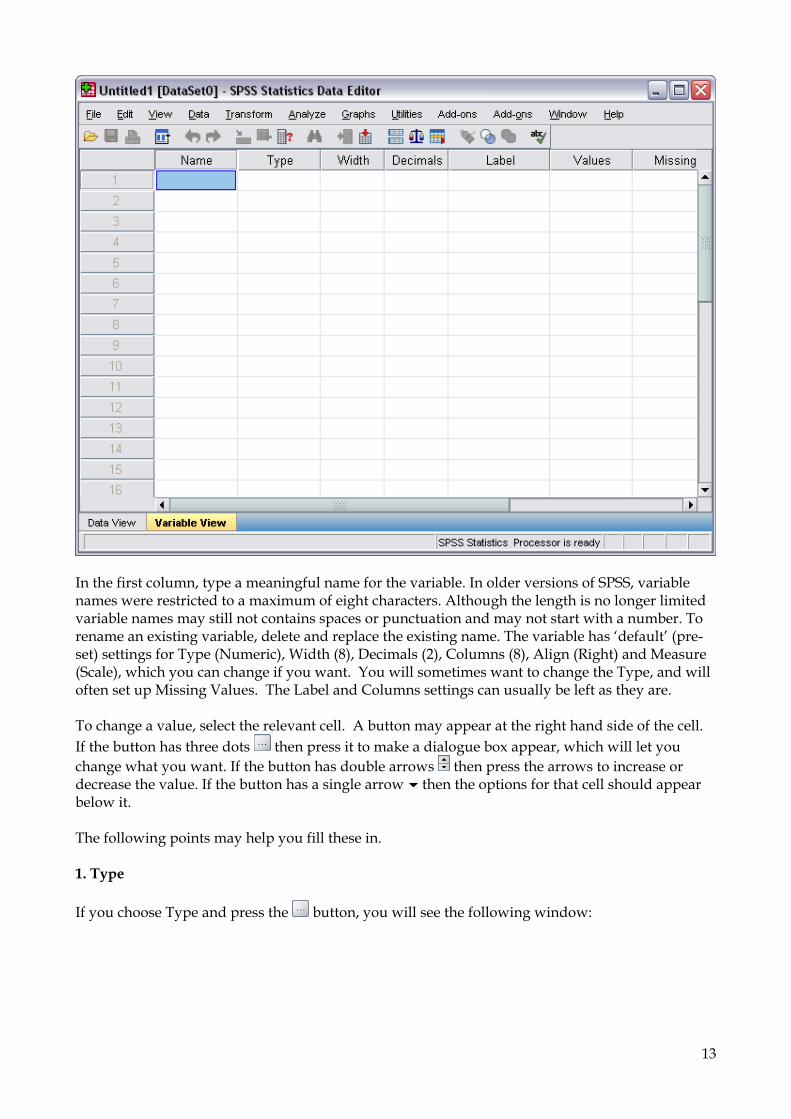
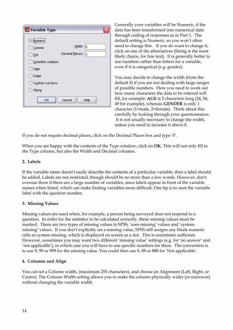
In the first column, type a meaningful name for the variable. In older versions of SPSS, variable names were restricted to a maximum of eight characters. Although the length is no longer limited variable names may still not contains spaces or punctuation and may not start with a number. To rename an existing variable, delete and replace the existing name. The variable has ‘default’ (pre-set) settings for Type (Numeric), Width (8), Decimals (2), Columns (8), Align (Right) and Measure (Scale), which you can change if you want. You will sometimes want to change the Type, and will often set up Missing Values. The Label and Columns settings can usually be left as they are. To change a value, select the relevant cell. A button may appear at the right hand side of the cell. If the button has three dots then press it to make a dialogue box appear, which will let you change what you want. If the button has double arrows then press the arrows to increase or decrease the value. If the button has a single arrow then the options for that cell should appear below it. The following points may help you fill these in. 1. Type If you choose Type and press the button, you will see the following window:

14

Generally your variables will be Numeric, if the data has been transformed into numerical data through coding of responses as in Part 1. The default setting is Numeric, so you won’t often need to change this. If you do want to change it, click on one of the alternatives (String is the most likely choice, for free text). It is generally better to use numbers rather than letters for a variable, even if it is categorical (e.g. gender). You may decide to change the width (from the default 8) if you are not dealing with large ranges of possible numbers. Here you need to work out how many characters the data to be entered will fill, for example: AGE is 2 characters long (24, 56, 49 for example), whereas GENDER is only 1 character (1=male, 2=female). Think about this carefully by looking through your questionnaires. It is not usually necessary to change the width, unless you need to increase it above 8.

If you do not require decimal places, click on the Decimal Places box and type ‘0’. When you are happy with the contents of the Type window, click on OK. This will not only fill in the Type column, but also the Width and Decimal columns. 2. Labels If the variable name doesn't easily describe the contents of a particular variable, then a label should be added. Labels are not restricted, though should be no more than a few words. However, don't overuse them if there are a large number of variables, since labels appear in front of the variable names when listed, which can make finding variables more difficult. One tip is to start the variable label with the question number. 3. Missing Values Missing values are used when, for example, a person being surveyed does not respond to a question. In order for the statistics to be calculated correctly, these missing values must be marked. There are two types of missing values in SPSS, ‘user-missing’ values and ‘system-missing’ values. If you don’t explicitly set a missing value, SPSS still assigns any blank numeric cells as system missing, which is displayed on screen as a dot. This is sometimes sufficient. However, sometimes you may want two different ‘missing value’ settings (e.g. for ‘no answer’ and ‘not applicable’), in which case you will have to use specific numbers for them. The convention is to use 9, 99 or 999 for the missing value. You could then use 8, 88 or 888 for 'Not applicable'. 4. Columns and Align You can set a Column width, (maximum 255 characters), and choose an Alignment (Left, Right, or Centre). The Column Width setting allows you to make the column physically wider (or narrower) without changing the variable width.

15

5. Measure The default type of measure is Scale for Numeric variables and Nominal for String variables. It is good practice at this point to check that you understand the way each variable is measured. • Scale: This is known in statistics as 'interval'. The actual numbers used and the gaps between

them have meaning. Examples include all measured quantities (height, weight, time, speed, etc) and standardised scales (IQ). Interval scales where the value '0' implies a total lack of the quantity measured are also known as 'ratio'. For example IQ and temperature in Celsius are interval, whereas reaction time and temperature in Kelvin are ratio. In this case age, bikeage, busage, etc. are scale variables.

• Ordinal: The numbers themselves are arbitrary, but the order in meaningful. This type of measurement is often used in Psychology and especially in questionnaires, since it includes Likert scales (rating scales) and other subjective scales. Technically, if the dependent variable in an analysis is ordinal, then a non-parametric test should be used. However, the rules of statistics are often 'bent' and ordinal variables are considered to be interval and then parametric tests are used. In this case driving, oxcity, mapread & spatial are ordinal variables, as are all the variables on the second page of the questionnaire.

• Nominal: This is also referred to as 'categorical'. The numbers used are simply labels for categories which cannot be placed in a meaningful order. For example, whereas 'Yes - Unsure - No' could be considered ordinal, 'Yes - Sometimes - Unsure - No' would have to be considered categorical since it could equally be written 'Yes - Unsure - Sometimes - No'. If a nominal variable contains only two categories (e.g. gender or 'Yes - No') then it can be considered to be ordinal, but should not be considered to be interval. Because gender only has two valid categories, it can be counted as ordinal. '1=Yes, 2=Unsure, 3=No' could be counted as ordinal, but '1=Yes, 2=No, 3=Unsure' could not.

6. Values If you choose Values and press the button, you will see the following window:

You can also add Value Labels, such as 1 for Male, 2 for Female. These are optional, but I recommend them as they will help you to make sense of your results. Adding value labels basically involves typing in a verbal description of each value of a particular variable, this will appear on any subsequent print outs.

16

4.1.2 To add a Value Label

1.

Click in the Value box and type the value you want to give a name to. Example: 1

2. Click in the Value Label box and type the label you want to associate with this value. Example: Male

3. Click on Add to add this relationship to the empty box at the bottom.

4. Repeat steps 1 to 3 until you have added all the Value Labels you want for this field.

5. Click on the Spelling… button if you want to check the spellings of your labels.

6. Click on the OK button to close the box.

Example: Value labels for OXCITY

1 Not at all 2 Not very 3 Somewhat 4 Quite 5 Very

4.2 Editing a Variable To alter a variable’s settings, simply change to Variable View and select the element you wish to change. Then proceed as above. NB: You can change the variable name if you want, without losing data.

4.3 Saving your data NOTE: this section covers saving your data. If you want to open a file you have already saved, see section 6.1, ‘Opening your data file’. Data should be saved early and often. A good rule of thumb is to save as soon as you start to feel that it would be painful to have to do again the work since your last save. This might be every few minutes, if your work is tricky or repetitive. Even if all you have done is define a few variables, it is worth saving now.

17

4.3.1 To save your data for the first time

1.

Make sure the Data window is ‘active’, i.e. in front of any other windows. (It is titled Untitled1 if you haven’t saved anything yet.)

2. From the File menu, select Save As

This brings up a dialogue box called Save Data As, with the ‘File Name’ box ready to accept your filename.

3.

Change the Drives window to H: (if it is not pointing there already).

4. Type the filename (preferably avoiding using punctuation) and click on OK (or press Enter ↵).

Example: TRAVEL01↵

If you want to save to a USB drive, make sure there is one connected to the computer, and type: E:\TRAVEL01↵ (or whatever drive letter the USB drive is using)

Do not use diskettes unless absolutely necessary. They are slow and unreliable. If you want to take your data home and do not have a USB drive then you can email the data to yourself. Some computers have CD or DVD writers, but the discs can get scratched or fail.

A word about file names There are a few things to take into account when choosing names for files. These points apply to almost all Windows programs, not just SPSS. Although modern versions of Windows allow filenames which break the following rules, it is still a good policy to bear them in mind when naming files. This reduces the risk of problems if you use different PCs, or email data files as attachments. File names can have one or two parts, separated by a dot (i.e. a full stop); the dot and the second part are optional. The first part can be up to 8 characters, the second part may be up to three; this is known as the 8.3 format. A file name can include letters and numbers, and certain punctuation characters such as ‘_’ (underscore) and ‘-‘ (hyphen), but not ‘/’ (slash) or ‘\’ (backslash). Legal file names include: X, FILENAME.DOC, PART_1.DK, MYFILE, DK970128. Illegal file names include: NAMETOOLONG, PART/1.DOC (slash not allowed), SECTION2.1.LST (only one dot allowed). As a general rule, you should confine yourself to choosing only the first 8 letters, and let SPSS (or any other application program) add the 3-character extension. Most programs add the extension themselves, and this helps programs to find their own files. (Many programs cannot open files created by other programs.) For example, Word adds DOC to your 8 character name, Excel adds XLS. SPSS adds SAV if it’s a data file, SPO if it’s an output file. This allows you to have the same name for two or more related files, such as ANOVA2.SAV for the data and ANOVA2.SPO for the output file. It also allows you to see which file was created by which program when you are looking at the files in your home directory.

18

4.3.2 Saving your data after the first save When you save your data for the first time, you have to give SPSS a file name. Subsequently, you only have to tell SPSS to save your file; it will save it with the same name.

1.

Make sure the Data window is ‘active’, i.e. in front.

2. From the File menu, select Save.

This saves the latest version of your work. The keyboard shortcut is Alt-F, S. It only takes a second!

OR from the File menu, select Exit to leave SPSS. When SPSS asks if you want to save your file before exiting, click on Yes and give a file name if necessary.

------------ ------------ Set up your data file, adding value labels where required. Save it with a name you are likely to remember! The filename TRAVEL01 reminds you that it was a travel questionnaire, and this is version 1.

19

5. Entering data Now you have set up your variables, and saved the file, you can start entering data. The variable names are listed across the top of the spreadsheet, and the Subject or Case number down the left hand side. To enter your data you need to insert each subject’s response to each question in the relevant cell. The raw data for this example is in the Appendix.

5.1 Data input Assemble your raw data, and type it in as follows: Note: The active cell - the cell into which anything you type will go, and marked by a bold line around the cell box - is initially, by default, the top left cell.

1.

Make sure you are looking at the Data View in the Data Editor. If you are looking at the Variable View then swap by selecting the Data View tab in the bottom left hand corner, or from the View menu, select Variables.

2.

Enter the value for the first case’s first variable. Don’t press the Enter (↵) key unless you want to move down a column; it is more likely that you will want to enter data by case than by variable.

In the example, the code of the first respondent is 1.

3. Press the Tab key (usually marked something like this: →⏐ and found to the left of the letter Q) OR the right-arrow (→) to move to the next variable (column) in the same case (row).

4. Using your questionnaire key, enter the relevant values for the first subject (case) into each column. Press →⏐ (Tab) or → (right-arrow) after each value to move to the next cell. Press the Home key to return to the start of the row.

N.B. Make sure you don’t go past the last variable column when you get to the right hand end of your spreadsheet. If you enter a value in a column which has not been set up to contain a variable, SPSS may automatically create a new variable called VAR0001, and you will have to delete the variable. See section 5.3, ‘Avoiding repetitive work when defining variables’.

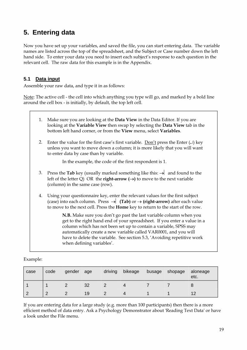
Example:

case code gender age driving bikeage busage shopage aloneage etc.

1 1 2 32 2 4 7 7 8

2 2 2 19 2 4 1 1 12 If you are entering data for a large study (e.g. more than 100 participants) then there is a more efficient method of data entry. Ask a Psychology Demonstrator about 'Reading Text Data' or have a look under the File menu.

20

NB. If you are not that familiar with the keyboard you may not know about the Number Pad on the right hand side. When entering large amounts of numbers, it is much faster to use the Number Pad rather than the numbers ranged above the letters. The Number Pad keys act as numbers if the green Num. Lock light is on, and as cursor control keys if the light is off. If the Num. Lock light is off, press the Num. Lock key and it should go on. You can then type in your data. If you want to return the numeric keypad to cursor control, press Num. Lock again to switch the Num. Lock light off. If you need to delete a variable (column) or case (row) you have created accidentally, see section 5.4, ‘To delete a variable (column) or case (row)’. Don’t forget to save your valuable data regularly!

5.2 Moving around the spreadsheet To move around the data entry spreadsheet i) Moving to a visible cell:

Click on the cell

ii) Moving to a particular case: From the Data menu, select Go to Case, type in the number of the case, and click on OK or press Enter (↵)

iii) Moving to a particular variable

Click on the button marked with a question mark near the middle of the toolbar. Click on the variable name you want to go to, then on the Go To button.

5.3 Avoiding repetitive work when defining variables In the Variable View you can copy and paste the contents of any of the definition cells, just as you might copy and paste numbers in the Data View.

5.4 To delete a variable (column) or case (row)

1. To make it easy to recover from a mistake made when deleting, save your file.

You can give it a new name (e.g. TRAVEL07 if previous version was TRAVEL06) if you want to make sure that previous versions of the file are not overwritten.

2.

Click on the variable name (or case number).

The whole column or row will become highlighted. Don’t do this by highlighting the individual cells or the next step will only delete the data, not the variable (or case) itself.

3.

Press Delete (or Del) on the keyboard.

After a few moments, the column or row will disappear.

21

NOTE: If you realise you have deleted the wrong variable, you can recover it by selecting Edit, then Undo. If you don’t do this immediately after deleting, you will not be able to get it back. The only way round this is be to reopen your most recently saved file, and hope your last save wasn’t too long ago! If this option is not available, you will have to Open the file you saved in step 1.

5.5 Finishing data entry When you have entered all your cases, SAVE YOUR DATA FILE. (See section 4.3, ‘Saving your data’.) If you want to start your analysis now, continue to Section 6. If you want to carry on later, then exit from SPSS for Windows (section 3.1.2, ‘Getting out of SPSS for Windows). If you have finished with the computer, log off the system.

22

6. Descriptive analysis using SPSS The following sections demonstrate how to analyse your data using SPSS. As for the other functions, this mainly involves choosing items from menus and submenus.

6.1 Opening your data file To open your file you need to be in SPSS for Windows.

1. Click on File, and select Open.

2. Select Data from the Open submenu

The Open Data File dialogue box appears.

3. Navigate to the correct drive (e.g. your home directory/H: drive or USB stick)

4. Type the name of the file (you don’t need to type the SAV; SPSS will automatically add it): e.g. TRAVEL01 OR Select the file from the list. Use the vertical scroll bar if your file is not in the list

5. Click on OK, or press Enter (↵)

6.2 Where does the output go to? When you run statistical analyses on your data, the results are displayed in the Output window. When you have run your analysis, you can switch to the Output window to examine, edit, save, copy or print your results.

6.3 Frequencies and means These are often overlooked as people rush to do more complicated analyses, but you will get a much better feel for your data if you first look at how the responses to each variable are distributed, and, where applicable, the variable means, standard deviations and ranges.

23

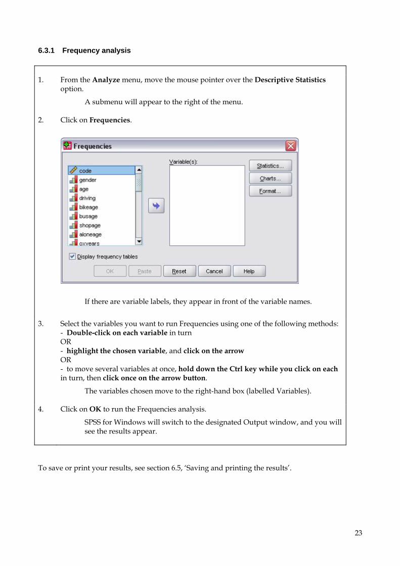
6.3.1 Frequency analysis 1. From the Analyze menu, move the mouse pointer over the Descriptive Statistics

option.

A submenu will appear to the right of the menu.

2. Click on Frequencies.

If there are variable labels, they appear in front of the variable names.

3. Select the variables you want to run Frequencies using one of the following methods:

- Double-click on each variable in turn OR - highlight the chosen variable, and click on the arrow OR - to move several variables at once, hold down the Ctrl key while you click on each in turn, then click once on the arrow button.

The variables chosen move to the right-hand box (labelled Variables).

4. Click on OK to run the Frequencies analysis.

SPSS for Windows will switch to the designated Output window, and you will see the results appear.

To save or print your results, see section 6.5, ‘Saving and printing the results’.

24

6.3.2 Calculating mean, range and standard deviation 1. From the Analyze menu, choose Descriptive Statistics.

2. Click on Descriptives.

3. Select the variables you want to analyse (as in section 6.3.1, ‘Frequency analysis’).

For example, in the travel questionnaire, we could look at the mean age, the mean ages of the various areas of freedom, and the mean score on some of the Likert type questions. The following variables will be used: AGE, BIKEAGE, BUSAGE, SHOPAGE, ALONEAGE, OXCITY, MAPREAD, SPATIAL.

4. Click on the Options button.

25

5. Check that the boxes next to Mean, Standard Deviation, Minimum and Maximum have been selected (this is the default).

Or pick other measures of central tendency, distribution and dispersion.

6. Check that the Display Order is Variable list if you want the output in the order you entered the variables.

Or pick other display orders.

7. Click on Continue to close the ‘Descriptives: Options’ dialogue box and return to the ‘Descriptives’ box.

8. Click on OK to run the analysis.

The results will appear in the designated Output window. To save or print your results, see section 6.5, ‘Saving and printing the results’.

6.4 Interpretation of results

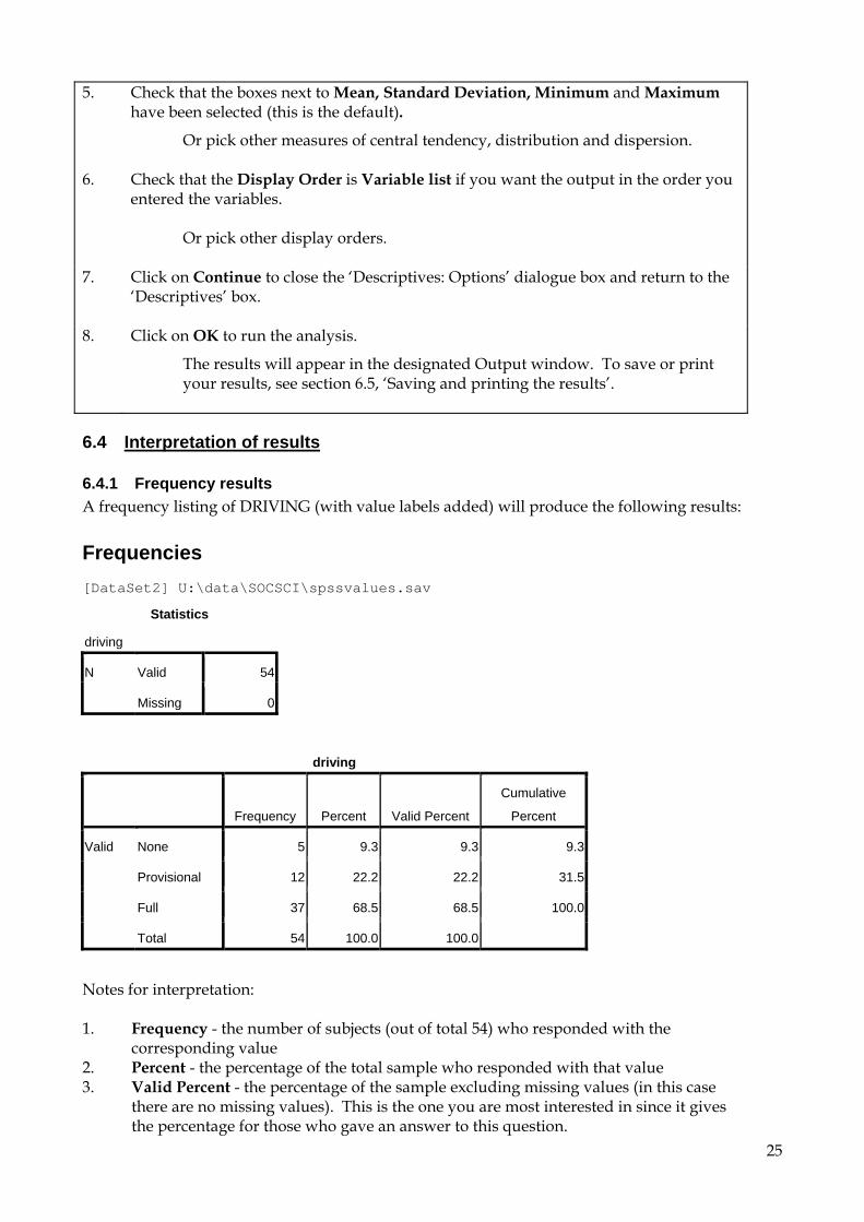
6.4.1 Frequency results A frequency listing of DRIVING (with value labels added) will produce the following results: Frequencies [DataSet2] U:\data\SOCSCI\spssvalues.sav

Statistics

driving

N Valid 54

Missing 0

driving

Frequency Percent Valid Percent

Cumulative

Percent

Valid None 5 9.3 9.3 9.3

Provisional 12 22.2 22.2 31.5

Full 37 68.5 68.5 100.0

Total 54 100.0 100.0

Notes for interpretation: 1. Frequency - the number of subjects (out of total 54) who responded with the

corresponding value 2. Percent - the percentage of the total sample who responded with that value 3. Valid Percent - the percentage of the sample excluding missing values (in this case

there are no missing values). This is the one you are most interested in since it gives the percentage for those who gave an answer to this question.

26

4. Cumulative Percent - the cumulative percentage i.e. the sum of the valid percentages of those value 1 + value 2, then value 1 + value 2 + value 3 etc. (This excludes missing values). Used for example to say: 31.5% do not have a full driving licence.

6.4.2 Descriptive statistics results A listing of the variable mentioned above would give the following results: Descriptives [DataSet1] U:\data\SOCSCI\spssraw.sav

Descriptive Statistics

N Minimum Maximum Mean Std. Deviation

age 54 18 57 24.31 8.147

driving 54 0 2 1.59 .659

bikeage 51 2 12 5.47 2.139

busage 54 1 16 11.07 2.346

shopage 54 1 18 10.67 2.761

aloneage 54 4 20 14.17 3.441

oxyears 54 0 28 2.48 5.421

oxmonths 54 0 201 9.46 26.814

oxcity 54 1 5 3.37 1.015

mapread 54 1 5 3.43 1.021

spatial 54 1 5 3.00 1.009

Valid N (listwise) 51 These results are fairly self-explanatory, giving in the following order: the variable name, the number of respondents excluding missing data (i.e. those who actually replied to this question), the minimum or lowest value occurring in the data, the maximum or highest value, the mean, and the standard deviation. The above table suggests that the data needs to be 'cleaned', since no child is going to travel on a bus or go to the shop alone at 1 year old. The results of the cleaned data look like this: Descriptives [DataSet2] U:\data\SOCSCI\spssvalues.sav

27

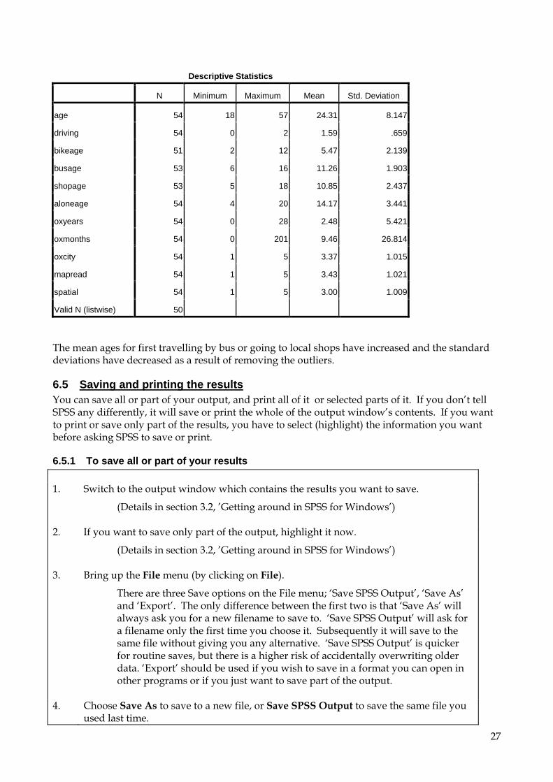
Descriptive Statistics

N Minimum Maximum Mean Std. Deviation

age 54 18 57 24.31 8.147

driving 54 0 2 1.59 .659

bikeage 51 2 12 5.47 2.139

busage 53 6 16 11.26 1.903

shopage 53 5 18 10.85 2.437

aloneage 54 4 20 14.17 3.441

oxyears 54 0 28 2.48 5.421

oxmonths 54 0 201 9.46 26.814

oxcity 54 1 5 3.37 1.015

mapread 54 1 5 3.43 1.021

spatial 54 1 5 3.00 1.009

Valid N (listwise) 50 The mean ages for first travelling by bus or going to local shops have increased and the standard deviations have decreased as a result of removing the outliers.

6.5 Saving and printing the results You can save all or part of your output, and print all of it or selected parts of it. If you don’t tell SPSS any differently, it will save or print the whole of the output window’s contents. If you want to print or save only part of the results, you have to select (highlight) the information you want before asking SPSS to save or print.

6.5.1 To save all or part of your results 1. Switch to the output window which contains the results you want to save.

(Details in section 3.2, ’Getting around in SPSS for Windows’)

2. If you want to save only part of the output, highlight it now.

(Details in section 3.2, ’Getting around in SPSS for Windows’)

3. Bring up the File menu (by clicking on File).

There are three Save options on the File menu; ‘Save SPSS Output’, ‘Save As’ and ‘Export’. The only difference between the first two is that ‘Save As’ will always ask you for a new filename to save to. ‘Save SPSS Output’ will ask for a filename only the first time you choose it. Subsequently it will save to the same file without giving you any alternative. ‘Save SPSS Output’ is quicker for routine saves, but there is a higher risk of accidentally overwriting older data. ‘Export’ should be used if you wish to save in a format you can open in other programs or if you just want to save part of the output.

4. Choose Save As to save to a new file, or Save SPSS Output to save the same file you

used last time.

28

5. If SPSS prompts you to save into ‘My Documents’ or on the U: drive, then change the

drive to H: and double-click on your student ID. Then type a filename using a maximum of eight characters (you don’t have to type the ‘SPV’ - SPSS for Windows will do that automatically), and click on OK.

6. SPSS will save your output as a ‘viewer’ file. If you wish to have a file which can be read by other programs (either plain text or hypertext format), then you must use Export rather than Save from the file menu. This will also allow you to save selected areas, rather than the whole output.

6.5.2 To print all or part of your results 1. Switch to the output window which contains the results you want to print.

(See section 3.2, ’Getting around in SPSS for Windows’ if you need to remind yourself how to do this.)

2. SPSS Output contains black squares down the left hand side which tell the printer to start a new page. If you want to save money and paper (but risk having tables spanning across two pages) then you should delete all of these black squares.

3. If you want to print only part of the output, highlight it now.

(Details in section 3.2, ’Getting around in SPSS for Windows’)

4. Click on the File menu, then on Print.

If you have highlighted some text, the ‘Selection’ option will already be marked (you can change this by clicking on the ‘All’ option). If you have not highlighted anything, you will be unable to choose ‘Selection’.

You can also choose the number of copies here; simply click in the ‘Copies’ box and type in the required number of copies.

5. Click on OK and the results will print.

29

7. Selecting sub-groups for analysis In the course of your analysis you may find that you want to run some statistics on a particular subgroup of subjects (for example, males only, or females under 21). You will therefore need to specify some criterion or criteria on which SPSS will either include or exclude cases. The following sections show how this works, using examples from the Travel questionnaire.

7.1 Select Cases

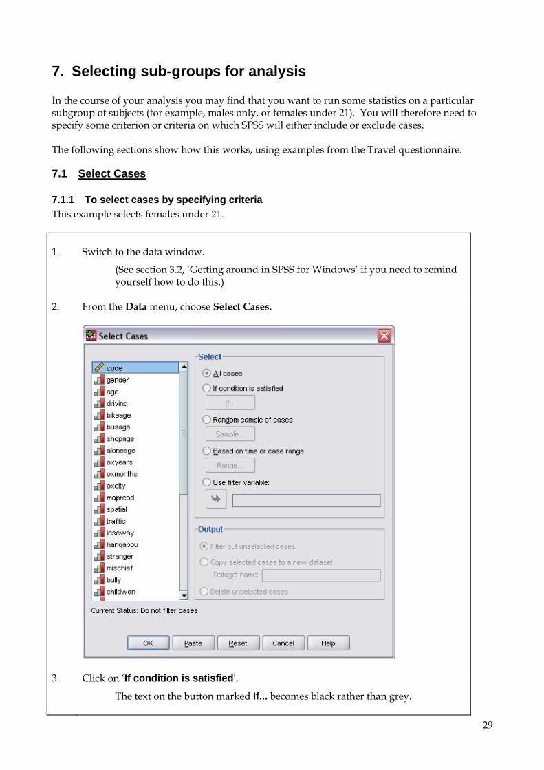
7.1.1 To select cases by specifying criteria This example selects females under 21. 1. Switch to the data window.

(See section 3.2, ’Getting around in SPSS for Windows’ if you need to remind yourself how to do this.)

2. From the Data menu, choose Select Cases.

3. Click on ‘If condition is satisfied’.

The text on the button marked If... becomes black rather than grey.

30

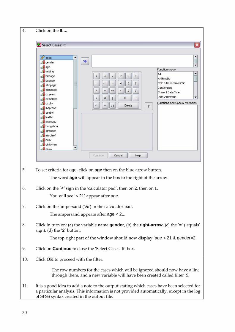
4. Click on the If....

5. To set criteria for age, click on age then on the blue arrow button.

The word age will appear in the box to the right of the arrow.

6. Click on the ‘<‘ sign in the ‘calculator pad’, then on 2, then on 1.

You will see ‘< 21’ appear after age.

7. Click on the ampersand (‘&’) in the calculator pad.

The ampersand appears after age < 21.

8. Click in turn on: (a) the variable name gender, (b) the right-arrow, (c) the ‘=‘ (‘equals’ sign), (d) the ‘2’ button.

The top right part of the window should now display ‘age < 21 & gender=2’.

9. Click on Continue to close the ‘Select Cases: If’ box.

10. Click OK to proceed with the filter.

The row numbers for the cases which will be ignored should now have a line through them, and a new variable will have been created called filter_$.

11. It is a good idea to add a note to the output stating which cases have been selected for a particular analysis. This information is not provided automatically, except in the log of SPSS syntax created in the output file.

31

NOTE: Until you change your criteria, subsequent analyses will apply only to the cases matching your criteria. To return to using all cases again, see section 7.1.2, 'To Return to using all cases’. If you look back at your Data window, you will see that some case numbers have an oblique line through them. These are the ones which do not match your selection criteria.

7.1.2 To return to using all cases 1. Switch to the data window.

(See section 3.2, ’Getting around in SPSS for Windows’ if you need to remind yourself how to do this.)

2. From the Data menu, choose Select Cases.

The ‘Select Cases’ dialogue box will appear. (See section 7.1.1, ‘To select cases by specifying criteria’ for an image of the box.)

3. Click on All cases.

4. Click on OK.

Subsequent analyses will operate on all cases. There should now be no oblique lines through the case numbers in the Data window.

7.1.3 To reapply the same criteria Repeat steps 1 to 3 in section 7.1.1, ’To select cases by specifying criteria’. You should find that your criteria appear next to the If... button, but ‘greyed out’, which means they are not active. All you need to do to use the same criteria is click on If condition is satisfied, and they will become active again (shown by turning black). You can also select Use filter variable and choose the variable filter_$ which will have been automatically created.

7.2 Split File If you wish to run the same analysis on two or more sub-groups then you could use Select Cases for each sub-group but a more efficient method is to split the file instead. Once the file has been split, any analysis will be conducted on each group separately.

7.2.1 To split the data file using a grouping variable 1. Switch to the data window.

2. From the Data menu, choose Split File.

32

3. Click on ‘Organise output by groups’.

The arrow on the button in the centre of the dialogue box becomes blue rather than grey.

4. To analyse male and female participants separately, click on gender then on the

right-arrow button.

The word gender will appear in the ‘Groups based on’ box to the right of the arrow.

5. Click on OK.

Any analysis conducted on the data with split file on will appear in the output separately for males and females. If desired, more than one grouping variable can be used at the same time, in which case every combination of the grouping variables will be analysed. Do not use any of the grouping variables in any analysis or dialogue boxes while the spit file is on. To return to analysing all cases, click on ‘Analyze all cases, do not create groups’. You do not need to remove variables from the ‘Groups based on’ box.

33

8. Modifying data While analysing your data you may find that you need to alter the way in which a variable is coded, for example, reversing the values, or grouping sets of values. In addition you may find that you need to create one or more new variables. There are two features in SPSS for Windows with which you can modify your data: Recode allows you to change the coding scheme for a variable, by for example combining several categories into one, or changing codes. You can recode into the existing variable, or create new ones. Compute allows you to combine values from more than one variable, or perform some mathematical change on the data in a variable. It may also be used to create a new variable, prior to changing the data (perhaps using Recode).

8.1 Recode Recode has two main uses: i) grouping values in a variable ii) reversing values in a variable i) Grouping values This is useful for variables such as AGE, where you have a wide range of values which you want to reduce to a number of smaller groups containing a range of values. Recoding involves specifying the name of the variables(s) to be recoded, and a set of transformations by which the old values are to be recoded into new ones. Note: it is also worth specifying new value labels which apply to the new coding to avoid any confusion in interpreting results. See example in this section. ii) Reversing values Sometimes it may be necessary to reverse the scores of some questions. This is commonly the case where Likert-type questions have been used, since often in the original questionnaire agreeing to some statements is equivalent to disagreeing to others.

8.1.1 Modifying data using Recode The following example recodes the DRIVING field from 3 specific categories into two. The new categories will divide the respondents into those who have a full driving licence and those who don't. 1. Switch to the data window.

(See section 3.2, ’Getting around in SPSS for Windows’ if you need to remind yourself how to do this.)

2. From the Transform, choose Recode Into Different Variables.

34

You can recode into the same variable, in which case the new grouped values would overwrite the old. It is often a good idea, however, to leave the original data intact. This allows you to return to it if necessary (if only to recode into different groups). Also, the new variables you create give you a history of your analyses, and let you see how your ideas developed.

3. Click on ‘driving’ in the list of variables on the left, then on the right-pointing arrow.

The driving variable moves to the Numeric Variable -> Output box.

4. In the Output Variable area, click in the Name box and type a new variable name, such as drivegrp.

5. Click on the Change button.

The Numeric Variable -> Output box should now show driving -> drivegrp.

6. Click on the Old and New Values button.

35

7. Click on the option button marked Range: LOWEST through value:

and type 1 in the box.

This will group non drivers and those with a Provisional licence.

8. In the New Value area of the window, click on the input box to the right of the word Value and type 0.

The Add button becomes active (black on grey instead of grey on grey).

9. Click on the Add button.

In the Old -> New box, the line ‘Lowest through 1 -> 0 appears. The first recoding into a category is now done.

10. In the Old Value area, click on the Value option. In the input box, type 2.

11. In the New Value area, click in the input box and type 1.

12. Click on Add.

A new line for the category appears in the Old -> New box.

13. In this case there are only two groups to be created. If there were more, steps 10 to 12 should be repeated - using the appropriate input boxes - until all groups have been set up.

14. Click on Continue to close the dialogue box and return to the Recode into Different Variables window.

The Old and New Values are now set up.

15. Click on OK to close the box and run the analysis.

If you are not already in the Data window, switch to it now. You will see the new variable there on the far right, containing appropriate values based on your coded transformations. It is likely that the numerical format of the new variable is not exactly how you want it; for instance it may default to a width of 8, with 2 decimal places. This may be changed in the same way as any other variable; double-click on the variable name, and change the variable type. You may also want to change the column format if the column is too wide or narrow. It is also a good idea to add Value Labels to the new variable, so you can see later what the codes mean. This is done in the same way as adding value labels to variables you have created yourself. To check how to do this, see section 4.1.2, ‘To add a Value Label’. Recode examples i) Grouping When you recode, choose an appropriate name for your new variable; the first example shows the Recode into Different Variables window being used to recode age into agecat1 (for Age Category grouping no. 1). The next window shows how the Recode into Different Variables: Old and New

36

Values window should look when you have finished setting up the categories, and before you click on the Continue button. Subsequent examples show only the Old and New Values window for each Recode.

The above example sets up three age groups: 0-19, 20-23, and 24+. Note: When recoding, it is important to think about whether you have created groups of very different sizes, and the effect this could have on your data, and on the validity of statistical tests you might want to apply.

37

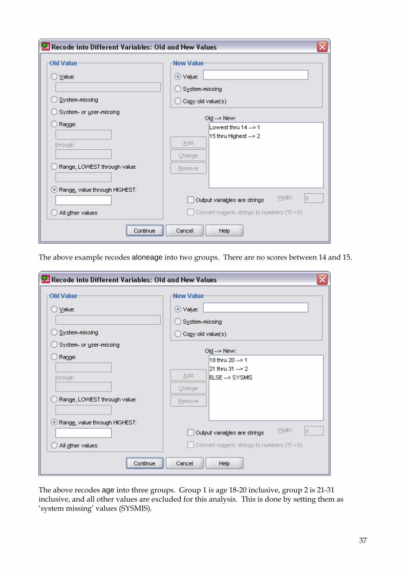
The above example recodes aloneage into two groups. There are no scores between 14 and 15.

The above recodes age into three groups. Group 1 is age 18-20 inclusive, group 2 is 21-31 inclusive, and all other values are excluded for this analysis. This is done by setting them as ‘system missing’ values (SYSMIS).

38

ii) Reversing values

The above example would reverse the values in a variable. In this questionnaire, there is no need to reverse any of the values, since all the Likert-type questions have been coded in the same way. If you want to recode two or more variables in the same way, you would set up the Old and New Values window as immediately above, and the Recode into Different Variables window as follows:

39

8.2 Compute Compute allows you to change values in a variable using mathematical functions or numeric expressions. You can store the results in the same variable, or a new one. Compute also provides a simple way to create a direct copy of a variable, in preparation for running analyses on the new variable without risking the original data.

8.2.1 To duplicate a variable using Compute 1. From the Transform menu, choose Compute Variable.

2. In the Target Variable box, type a name for your new variable.

Do not use spaces or punctuation in the new variable name.

3. In the list of variables at the bottom left of the box, click on the name of the variable you want to duplicate, and press the right arrow button.

The variable name appears in the Numeric Expression box.

4. Click on OK.

You now have a new variable holding exactly the same data as the old variable.

40

8.2.2 To combine values in two or more variables You can add values in two or more variables to give an overall score on a particular index. In the following example, a new variable called Skill2 combines responses on two different questions, both of which measure the individuals’ perception of their skill at handling a car at high speed. This is particularly useful if, for example, you have a number of knowledge-based questions which you want to combine to gain an overall knowledge score. But you need to think about whether the range of responses is the same on each item/question and if not, what effect this will have on any combined scoring system. 1. From the Transform menu, choose Compute Variable.

The Compute Variable dialogue box appears.

2. In the Target Variable box, type a name for your new variable, such as oxtime.

3. In the list of variables at the bottom left of the box, click on the first of the variables you want to use to create the new variable - in this case, oxyears, and press the right arrow button.

The variable name appears in the Numeric Expression box.

4. Click on the button marked ‘+’ at the top left of the calculator keypad.

A ‘+’ sign appears in the Numeric Expression box. You are now building an ‘expression’, using existing variables, which will specify the values in the new variable.

5. Click on the next variable you plan to use. For this example, use oxmonths.

The expression should now read: oxyears + oxmonths

6. Click on the button marked ‘/’ at the top of the calculator keypad and they type 12.

The expression should now read: oxyears + oxmonths/12

7. Click on OK.

The new variable, oxtime, will now be created. For each case it will contain the total number of years the respondent has lived in Oxfordshire. For example, if case 6 had 19 in oxyears, and 4 in oxmonths, the new value of oxtime will be 19.33.

If you are unsure about which order the components of an expression will be evaluated, use brackets.

41

8.3 More complex transformations using SPSS’s Command Language Say you want to set up the following groups for analysis: Group Made up of 1. Males, 21 years old or less 2. Females, 21 years old or less 3. Males, 22 and over 4. Females, 22 and over The best way to do this is to use the built-in SPSS command language. For most functions, selecting options from the menus is enough. However, for more complex transformations, the command language can be better, and may sometimes be necessary. Once you have created a command sequence, you can save it as a file, and recall it during a future session to run the same analysis, or change it to run a different one. Although it takes longer to set up an analysis using command language, it can save time in the long run, if you are running similar analyses repeatedly. It can also save time if you are running long sequences of transformations and analyses, when you can leave SPSS to get on with the work, rather than having to choose an option, then wait until it completes before starting the next. To create a command line, you have to be in a Syntax window.

8.3.1 Compute and Recode using command language 1. First, open a Syntax window: from the File menu, choose New.

2. From the submenu which appears, choose Syntax.

You will see a window titled ‘Syntax’ appear, containing two empty windows and the blinking cursor. This is the ‘blank paper’ on which you will write your command sequence.

3. Type the following into the right hand window, being careful to put the brackets in

the right place, and the full stop at the end of each line:

compute agesexgp=. if (age le 21 and gender=1) agesexgp=1. if (age le 21 and gender=2) agesexgp=2. if (age ge 22 and gender=1) agesexgp=3. if (age ge 22 and gender=2) agesexgp=4. execute.

The command (compute, if and execute) will automatically appear in the left hand box. It will be greyed out if SPSS does not recognise it.

The ‘le’ means ‘less than or equal to’ and the ‘ge’ signifies ‘greater than or equal to’. The first line creates a new variable called AGESEXGP (for Age/Sex Group).

The second and subsequent lines are run on every case, and say that, for any given case, if it fulfils the condition in the brackets, the value in the AGESEXGP variable for that case will be set by the ‘assignment’ on the second half of the same line.

42

So, the second line says: for the current case, if the AGE variable is less than or equal to 21, and the SEX variable equals 1, then the new value of AGESEXGP for this case is 1. The last line says: if AGE is 22 or more, and SEX is 2, then put 4 in the AGESEXGP variable for the current case.

The final line informs SPSS that you wish to proceed with the above calculations.

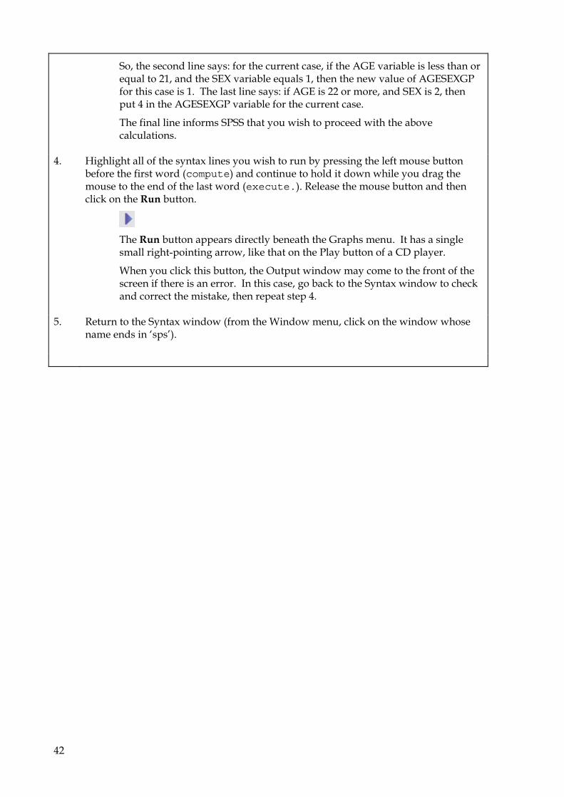
4. Highlight all of the syntax lines you wish to run by pressing the left mouse button

before the first word (compute) and continue to hold it down while you drag the mouse to the end of the last word (execute.). Release the mouse button and then click on the Run button.

The Run button appears directly beneath the Graphs menu. It has a single small right-pointing arrow, like that on the Play button of a CD player.

When you click this button, the Output window may come to the front of the screen if there is an error. In this case, go back to the Syntax window to check and correct the mistake, then repeat step 4.

5. Return to the Syntax window (from the Window menu, click on the window whose

name ends in ‘sps’).

43

8.4 Protecting your data from accidents

8.4.1 Running checks When you are doing many data transformations, it is easy to make an unintended change accidentally. The machine will do exactly as you command, which may sometimes not be what you wanted! This can happen especially when using commands, when a sequence may be syntactically correct (i.e., SPSS understands and runs it) but logically inaccurate (e.g. you stipulate ‘less than’ when you should use ‘less than or equal to’). This kind of thing is easy to miss until later. One protection against this is to run Descriptives periodically, to check that you get the same values that you did originally. If you do, then your data is safe. If the values have changed for variables that you haven’t intentionally altered, then you need check where the error is before proceeding. You may also need to rerun your most recent analyses and transforms again.

8.4.2 Saving modified data Recode and Compute alter or create variables for the duration of the current SPSS session. If you want to permanently Recode a variable, or to have access to a new variable, you must save the file.

8.4.3 The importance of backing up your data It is VERY IMPORTANT to keep the original raw data file unaltered, and to keep backup copies of your work. This means you always have access to the data taken directly from the questionnaires. You should also make one copy of the original file onto a USB drive as well as having another copy on your H: drive. Imagine the worst that might happen, and prepare for it; a few minutes’ work now might save hours later. If you need to go back to the original, don’t change it; simply make another copy and work from that. The reason for all this is that data loss can go undetected for a while, and you can find that the backups you were assiduously making were in fact overwriting good data with bad. You may need several ‘generations’ of backup to be sure that you can recover from potential disaster. Another good practice is to save your changed data with a new version number each time. For example, TRAVEL01, TRAVEL02 etc. (Use ‘01’ rather than just ‘1’ to allow for listing your files in name order; otherwise TRAVEL11 will come before TRAVEL2.) If you discover a problem with your data, you can go back through each version in turn until you find one you can trust. Although this runs the risk of taking up disk space on the system, you can always copy older files off the system onto a USB drive. Although all this does create an overhead, if you have ever suffered a data accident you will realise its virtue. Unfortunately, most people only learn this the hard way! Although USB drives (also known as pen drives or flash drives) are far more reliable than diskettes and CD-ROMs, you still should not trust them with your only copy of important files. In general extensions to coursework are not given because of data loss due to corrupt diskettes, etc.

44

9. Statistical analyses In this section we will be looking at some simple ways in which you can look at relationships between variables. You have already looked at the distribution of your questionnaire data. Now you are interested in how the different variables relate to each other, if indeed they do. When you designed your questionnaire you probably had some idea of the model which guided you, and some notion of which variables you might expect to be related. So, rather than comparing everything with everything else, go back to these original ideas or hypotheses to examine whether they are borne out by the data. There are a number of statistical tests for looking at relationships or differences. The tests covered here are: 1. Correlation (Pearson and Spearman) 2. Crosstabs (Chi-Square) 3. t-test 4. Non parametric tests 5. One-way Anova (Analysis of Variance) 6. Two-way Anova 7. Repeate Measures Anova 8. Multiple Regression 9. Factor Analysis 10. Reliability Analysis The choice of which test to do will depend on (a) what questions you are asking, (b) the type of data you have, and (c) your research design (for example, whether you have included repeated measure so the same thing on each subject, or whether you are looking at between-subject measures). The table below gives a simple guide to the use of these tests. For further explanation, refer to a statistics text book or the SPSS for Windows manual (normally available in room C223a).

MEASURING STATISTICAL ASSOCIATION

Correlation Calculates the Pearson’s correlation coefficient between pairs of two or more variables i.e. measure the strength of their linear association. If one or both of the variables are ordinal, a non parametric Spearman correlation should be used instead.

Crosstabs Equivalent to Chi-square test. Looks at the frequency distribution of individuals falling into each combination of two mutually exclusive and exhaustive categories e.g. sex. Estimates whether the observed frequencies differ significantly from those which would occur if the two variables were independent (i.e. unrelated).

COMPARING MEANS

t-test One-factor, 2 levels, independent or repeated measures. There are non parametric equivalents for both independent and paired t-tests.

Anova One or more factors, or more than 2 levels, independent, repeated or mixed measures. There are non parametric equivalents for single factor ANOVAs.

COMBINATION

Multiple Regression

One or more interval or ordinal variables with 2 or more ordered levels. Measures the strength of their multiple linear association.

45

NB: To use these tests the data must be approximately normally distributed (look at your data using Frequencies to check this). If your data are not normally distributed you need to use a non-parametric test. The SPSS manual is one source of information on non-parametric tests.

9.1 Correlation

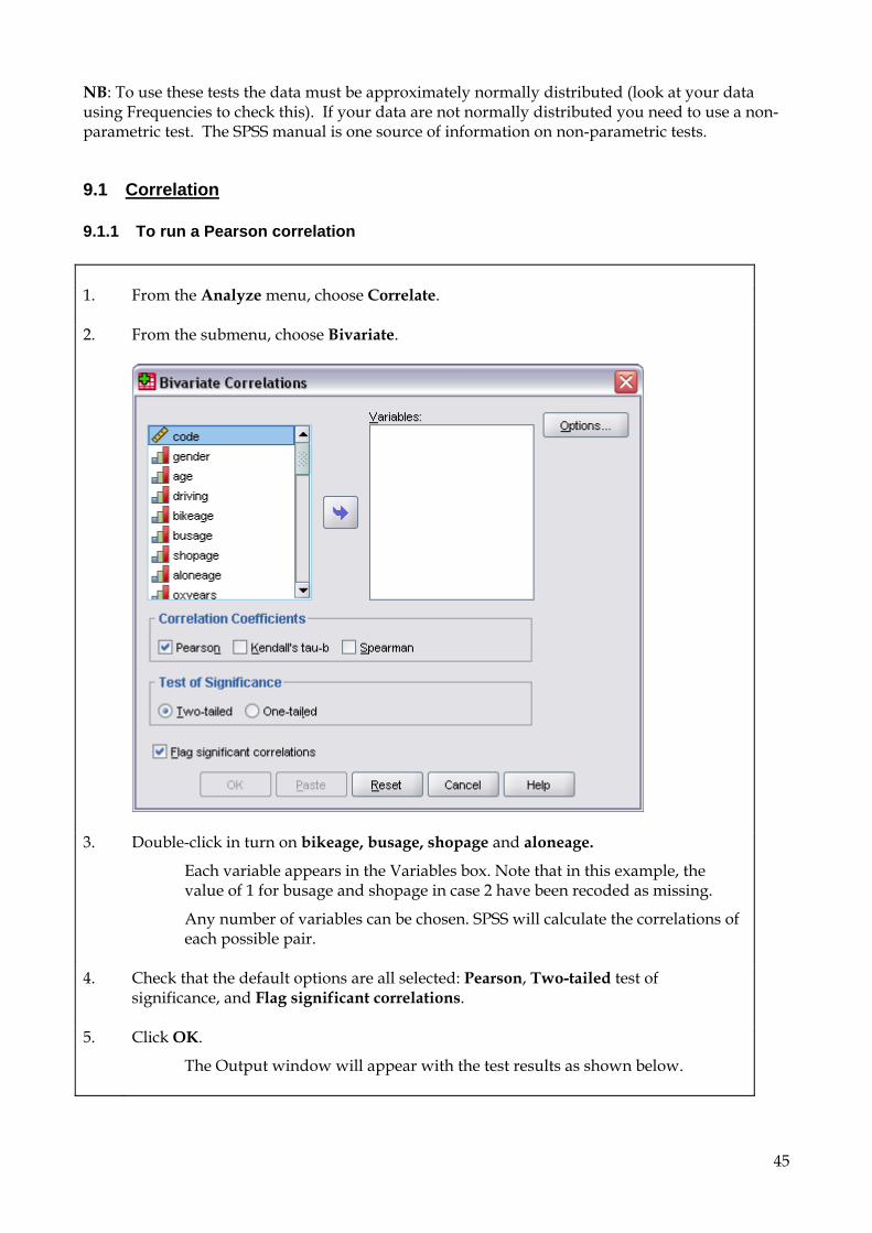
9.1.1 To run a Pearson correlation 1. From the Analyze menu, choose Correlate.

2. From the submenu, choose Bivariate.

3. Double-click in turn on bikeage, busage, shopage and aloneage.

Each variable appears in the Variables box. Note that in this example, the value of 1 for busage and shopage in case 2 have been recoded as missing.

Any number of variables can be chosen. SPSS will calculate the correlations of each possible pair.

4. Check that the default options are all selected: Pearson, Two-tailed test of

significance, and Flag significant correlations.

5. Click OK.

The Output window will appear with the test results as shown below.

46

Interpretation of correlation results, using the example above Since SPSS was asked to correlate three variables (questions 5, 8, and 9) the results appear as a correlation matrix listing the correlation coefficients between all three variables and each other: Correlations [DataSet1] U:\data\SOCSCI\spssvalues.sav

Correlations

bikeage busage shopage aloneage

bikeage Pearson Correlation 1 .117 .104 .009

Sig. (2-tailed) .420 .471 .952

N 51 50 50 51

busage Pearson Correlation .117 1 .718** .354**

Sig. (2-tailed) .420 .000 .009

N 50 53 53 53

shopage Pearson Correlation .104 .718** 1 .239

Sig. (2-tailed) .471 .000 .085

N 50 53 53 53

aloneage Pearson Correlation .009 .354** .239 1

Sig. (2-tailed) .952 .009 .085

N 51 53 53 54

**. Correlation is significant at the 0.01 level (2-tailed). Notes: 1. Significant correlations are marked with one or two stars after the calculated value. 2. The degrees of freedom for a correlation are n-2. 3. In this case, two correlations are significant at the .01 (**) level: one between

SHOPAGE and BUSAGE (r=.718; df=51; p<.001), and the other between BUSAGE and ALONEAGE (r=.354; df=51; p=.009). However, BIKEAGE does not correlate strongly with any of the other variables and the correlation between SHOPAGE and ALONEAGE is not significant at the 5% level. The two significant results show positive correlations (since the signs of the correlation coefficients are positive) meaning that as values for one variable increase, so do those for the other. In this case higher reported ages of first going to shops without an adult (SHOPAGE), and higher reported ages of first being allowed out alone (ALONEAGE) tend to correspond to higher reported ages of first travelling by bus without an adult (BUSAGE).

4. The square of the correlation value gives the proportion of overlapping variance between the two variables, and a standard measure of effect size. Therefore there is a 0. 516 (52%) overlap between SHOPAGE and BUSAGE, but only a 0.125 (13%) overlap between BUSAGE and ALONEAGE. The relationship between BUSAGE and SHOPAGE is four times stronger than the one between BUSAGE and ALONEAGE.

5. SPSS does not offer confidence intervals as an option for correlations.

47

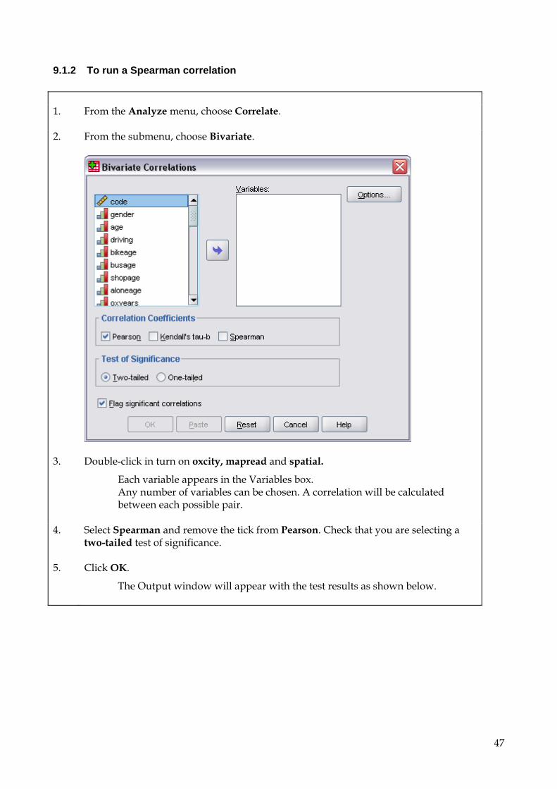
9.1.2 To run a Spearman correlation 1. From the Analyze menu, choose Correlate.

2. From the submenu, choose Bivariate.

3. Double-click in turn on oxcity, mapread and spatial.

Each variable appears in the Variables box. Any number of variables can be chosen. A correlation will be calculated between each possible pair.

4. Select Spearman and remove the tick from Pearson. Check that you are selecting a

two-tailed test of significance.

5. Click OK.

The Output window will appear with the test results as shown below.

48

Interpretation of correlation results, using the example above Since SPSS was asked to correlate three variables the results appear as a correlation matrix listing the correlation coefficients between all three variables and each other: Nonparametric Correlations [DataSet1] U:\data\SOCSCI\spssvalues.sav

Correlations

oxcity mapread spatial

Spearman's rho oxcity Correlation Coefficient 1.000 .344* .287*

Sig. (2-tailed) . .011 .035

N 54 54 54

mapread Correlation Coefficient .344* 1.000 .615**

Sig. (2-tailed) .011 . .000

N 54 54 54

spatial Correlation Coefficient .287* .615** 1.000

Sig. (2-tailed) .035 .000 .

N 54 54 54

*. Correlation is significant at the 0.05 level (2-tailed).

**. Correlation is significant at the 0.01 level (2-tailed). Notes: 1. Significance is indicated by the presence or absence of one or two stars after the

computed coefficient. 2. The degrees of freedom for a correlation are n-2. 3. In this case, one correlation is significant at the .01 (**) level: MAPREAD and

SPATIAL (ρ[52]=.615; p<.001). OXCITY shows weaker but still significant correlations with both MAPREAD (ρ[52]=.344; p=.011) and SPATIAL (ρ[52]=.287; p=.034). All three correlations are positive, which shows that participants who rated themselves more highly on one ability tend to also rate themselves more highly on the others.

49

9.2 Crosstabs and Chi-squared tests

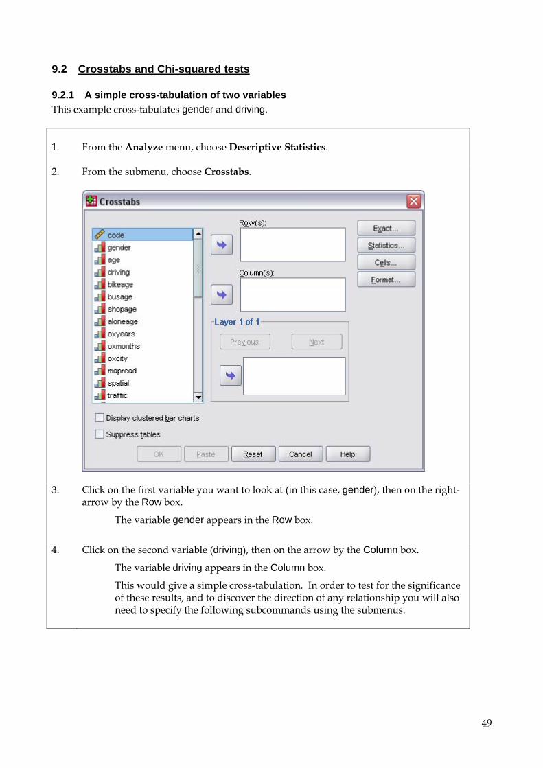
9.2.1 A simple cross-tabulation of two variables This example cross-tabulates gender and driving. 1. From the Analyze menu, choose Descriptive Statistics.

2. From the submenu, choose Crosstabs.

3. Click on the first variable you want to look at (in this case, gender), then on the right-arrow by the Row box.

The variable gender appears in the Row box.

4. Click on the second variable (driving), then on the arrow by the Column box.

The variable driving appears in the Column box.

This would give a simple cross-tabulation. In order to test for the significance of these results, and to discover the direction of any relationship you will also need to specify the following subcommands using the submenus.

50

5. Click on the Cells button.

6. Leaving the Observed box selected, click on Expected and Row to tick them, then on Continue.

‘Observed’ gives the numbers actually found. ‘Expected’ gives the numbers which would appear if the variables were independent, i.e. unrelated.

The Crosstabs: Cell Display box closes, and returns you to the Crosstabs dialogue box.

7. Click on the Statistics button.

51

8. Click on Chi-Square to select it, then on Continue.

You are returned to the Crosstabs window.

9. Click on OK to run the analysis.

Note: Since Crosstabs produces a table with cells showing each combination of two variables, it is only really suitable for use with variables with a modest number of categories (e.g. no more than five). In some cases you can first reduce the number of categories using Recode. Interpretation of results using sample questionnaire Example 1 These tables list the results of a crosstabulation between GENDER and DRIVING . Crosstabs [DataSet1] U:\data\SOCSCI\spssvalues.sav

Case Processing Summary

Cases

Valid Missing Total

N Percent N Percent N Percent

gender * driving 54 100.0% 0 .0% 54 100.0%

gender * driving Crosstabulation

driving

Total None Provisional Full

gender Male Count 0 3 4 7

Expected Count .6 1.6 4.8 7.0

% within gender .0% 42.9% 57.1% 100.0%

Female Count 5 9 33 47

Expected Count 4.4 10.4 32.2 47.0

% within gender 10.6% 19.1% 70.2% 100.0%

Total Count 5 12 37 54

Expected Count 5.0 12.0 37.0 54.0

% within gender 9.3% 22.2% 68.5% 100.0%

52

Chi-Square Tests

Value df

Asymp. Sig. (2-

sided)

Pearson Chi-Square 2.438a 2 .296

Likelihood Ratio 2.810 2 .245

Linear-by-Linear Association .008 1 .927

N of Valid Cases 54

a. 4 cells (66.7%) have expected count less than 5. The minimum

expected count is .65.

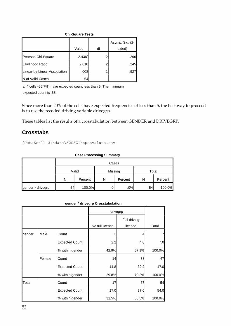
Since more than 20% of the cells have expected frequencies of less than 5, the best way to proceed is to use the recoded driving variable drivegrp. These tables list the results of a crosstabulation between GENDER and DRIVEGRP. Crosstabs [DataSet1] U:\data\SOCSCI\spssvalues.sav

Case Processing Summary

Cases

Valid Missing Total

N Percent N Percent N Percent

gender * drivegrp 54 100.0% 0 .0% 54 100.0%

gender * drivegrp Crosstabulation

drivegrp

Total No full licence

Full driving

licence

gender Male Count 3 4 7

Expected Count 2.2 4.8 7.0

% within gender 42.9% 57.1% 100.0%

Female Count 14 33 47

Expected Count 14.8 32.2 47.0

% within gender 29.8% 70.2% 100.0%

Total Count 17 37 54

Expected Count 17.0 37.0 54.0

% within gender 31.5% 68.5% 100.0%

53

Chi-Square Tests

Value df

Asymp. Sig. (2-

sided)

Exact Sig. (2-

sided)

Exact Sig. (1-

sided)

Pearson Chi-Square .482a 1 .487

Continuity Correctionb .067 1 .796

Likelihood Ratio .462 1 .497

Fisher's Exact Test .665 .384

Linear-by-Linear Association .474 1 .491

N of Valid Cases 54

a. 2 cells (50.0%) have expected count less than 5. The minimum expected count is 2.20.

b. Computed only for a 2x2 table Notes: 1. Testing the relationship:

The presence or absence of a relationship between the two variables is determined by the significance level. We are interested in the first figure given in the column labelled ‘Significance’ (i.e. the Pearson’s value). In this case the two variables are unrelated (χ2[1]=.482; p=.487). This result is not significant. However, in this case since there are still more than 20% of cells with expected counts of less than 5, the Fisher's Exact Test should be used instead (Fisher's Exact, p=.665). A p-value of .050 or less would suggest a significant relationship between the two variables, i.e. that they are not independent. The significance level alone does not tell you the direction of their relationship; in order to establish this you would need to look at the figures in the table.

2. Interpreting the table: The variables crosstabulated are listed along the top and down the side of the table, each cell therefore represents a different category combination defined by the gender of the respondent and the response to the DRIVING question.

3. The top number in each cell represents the number of cases who fall into that category combination i.e. the observed frequency. The second number is the expected frequency i.e. the number who would fall into each category combination if the two variables were independent; in other words, by chance. In order to establish the direction of the relationship (having established that they are indeed related) look at the difference between the observed and expected frequencies.

4. Observed and Expected frequencies vs. Percentages In a lab report it is not usual to present tables of observed and expected frequencies (although they are useful in establishing the direction of the relationship before writing up, as above). Instead, present a table of observed data expressed as numbers and percentages (i.e. the number of cases in each cell, and the same number expressed as a percentage) or just percentages. These figures can be worked out by hand, and/or selecting the options Row and Column, and deselecting Expected, in the Crosstabs: Cell Display window (at step 6 above). SPSS will calculate the observed

54

frequencies as percentages of the row and column totals in the table for you. Decide whether you wish to report Row percentages or Column percentages, but do not report both. When one of the categories (usually the one chosen as for the columns) only has two categories, percentages can be used to describe the data in the body of the text, without using a table at all. The above table shows that 57% of women and 70% of men hold full driving licences, but these percentages are not significantly different from each other (Fisher's Exact, p=.665).

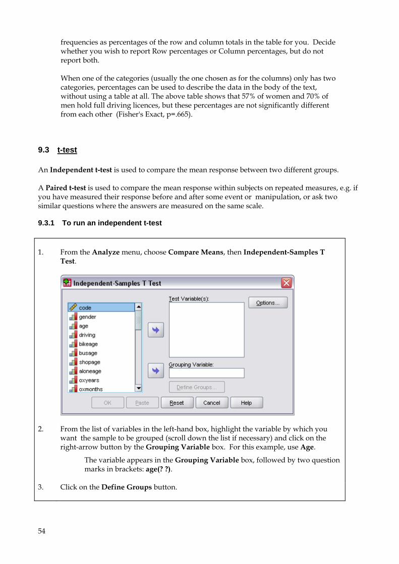
9.3 t-test An Independent t-test is used to compare the mean response between two different groups. A Paired t-test is used to compare the mean response within subjects on repeated measures, e.g. if you have measured their response before and after some event or manipulation, or ask two similar questions where the answers are measured on the same scale.

9.3.1 To run an independent t-test 1. From the Analyze menu, choose Compare Means, then Independent-Samples T

Test.

2. From the list of variables in the left-hand box, highlight the variable by which you want the sample to be grouped (scroll down the list if necessary) and click on the right-arrow button by the Grouping Variable box. For this example, use Age.

The variable appears in the Grouping Variable box, followed by two question marks in brackets: age(? ?).

3. Click on the Define Groups button.

55

In most cases the grouping variable (independent variable) will already contain single values to represent the two groups. If this is the case, just enter their values into the boxes labelled Group 1 and Group 2. In this case, however, the grouping variable is interval and so a cut point must be specified.

4. Select Cut point. In the Cut point box, type 21.

This will compare people who are under 21 with those who are 21 or over.

5. Click on Continue.

The display in the Grouping Variable box now shows age(21).

6. Highlight the variable or variables whose means you want to compare across the two groups (e.g. aloneage) and click on the right-arrow button by the Test Variable(s) box.

The variable name appears in Test Variable(s) the box.

7. Click on OK to run the test.

The results as shown below appear in the Output window.

Interpretation of results using sample questionnaire T-Test [DataSet1] U:\data\SOCSCI\spssvalues.sav

Group Statistics

age N Mean Std. Deviation Std. Error Mean

aloneage >= 21 28 13.14 4.249 .803

< 21 26 15.27 1.779 .349

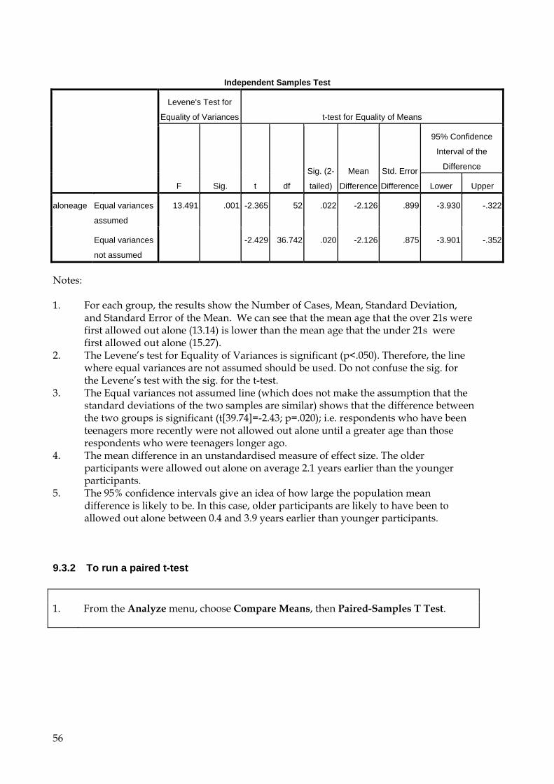
56

Independent Samples Test

Levene's Test for

Equality of Variances t-test for Equality of Means

F Sig. t df

Sig. (2-

tailed)

Mean

Difference

Std. Error

Difference

95% Confidence

Interval of the

Difference

Lower Upper

aloneage Equal variances

assumed

13.491 .001 -2.365 52 .022 -2.126 .899 -3.930 -.322

Equal variances

not assumed -2.429 36.742 .020 -2.126 .875 -3.901 -.352

Notes: 1. For each group, the results show the Number of Cases, Mean, Standard Deviation,

and Standard Error of the Mean. We can see that the mean age that the over 21s were first allowed out alone (13.14) is lower than the mean age that the under 21s were first allowed out alone (15.27).

2. The Levene’s test for Equality of Variances is significant (p<.050). Therefore, the line where equal variances are not assumed should be used. Do not confuse the sig. for the Levene’s test with the sig. for the t-test.

3. The Equal variances not assumed line (which does not make the assumption that the standard deviations of the two samples are similar) shows that the difference between the two groups is significant (t[39.74]=-2.43; p=.020); i.e. respondents who have been teenagers more recently were not allowed out alone until a greater age than those respondents who were teenagers longer ago.

4. The mean difference in an unstandardised measure of effect size. The older participants were allowed out alone on average 2.1 years earlier than the younger participants.

5. The 95% confidence intervals give an idea of how large the population mean difference is likely to be. In this case, older participants are likely to have been to allowed out alone between 0.4 and 3.9 years earlier than younger participants.

9.3.2 To run a paired t-test 1. From the Analyze menu, choose Compare Means, then Paired-Samples T Test.

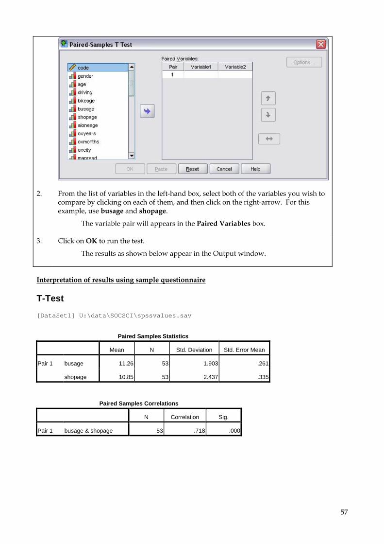
57

2. From the list of variables in the left-hand box, select both of the variables you wish to compare by clicking on each of them, and then click on the right-arrow. For this example, use busage and shopage.

The variable pair will appears in the Paired Variables box.

3. Click on OK to run the test.

The results as shown below appear in the Output window.

Interpretation of results using sample questionnaire T-Test [DataSet1] U:\data\SOCSCI\spssvalues.sav

Paired Samples Statistics

Mean N Std. Deviation Std. Error Mean

Pair 1 busage 11.26 53 1.903 .261

shopage 10.85 53 2.437 .335

Paired Samples Correlations

N Correlation Sig.

Pair 1 busage & shopage 53 .718 .000

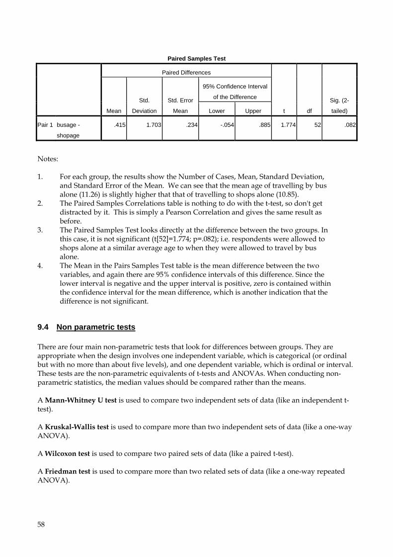
58

Paired Samples Test

Paired Differences

t df

Sig. (2-

tailed) Mean

Std.

Deviation

Std. Error

Mean

95% Confidence Interval

of the Difference

Lower Upper

Pair 1 busage -

shopage

.415 1.703 .234 -.054 .885 1.774 52 .082

Notes: 1. For each group, the results show the Number of Cases, Mean, Standard Deviation,

and Standard Error of the Mean. We can see that the mean age of travelling by bus alone (11.26) is slightly higher that that of travelling to shops alone (10.85).

2. The Paired Samples Correlations table is nothing to do with the t-test, so don't get distracted by it. This is simply a Pearson Correlation and gives the same result as before.

3. The Paired Samples Test looks directly at the difference between the two groups. In this case, it is not significant (t[52]=1.774; p=.082); i.e. respondents were allowed to shops alone at a similar average age to when they were allowed to travel by bus alone.

4. The Mean in the Pairs Samples Test table is the mean difference between the two variables, and again there are 95% confidence intervals of this difference. Since the lower interval is negative and the upper interval is positive, zero is contained within the confidence interval for the mean difference, which is another indication that the difference is not significant.

9.4 Non parametric tests There are four main non-parametric tests that look for differences between groups. They are appropriate when the design involves one independent variable, which is categorical (or ordinal but with no more than about five levels), and one dependent variable, which is ordinal or interval. These tests are the non-parametric equivalents of t-tests and ANOVAs. When conducting non-parametric statistics, the median values should be compared rather than the means. A Mann-Whitney U test is used to compare two independent sets of data (like an independent t-test). A Kruskal-Wallis test is used to compare more than two independent sets of data (like a one-way ANOVA). A Wilcoxon test is used to compare two paired sets of data (like a paired t-test). A Friedman test is used to compare more than two related sets of data (like a one-way repeated ANOVA).

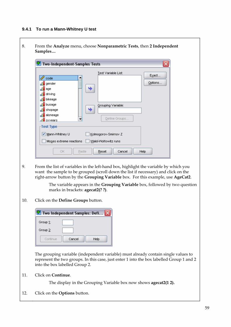
59

9.4.1 To run a Mann-Whitney U test 8. From the Analyze menu, choose Nonparametric Tests, then 2 Independent

Samples…

9. From the list of variables in the left-hand box, highlight the variable by which you want the sample to be grouped (scroll down the list if necessary) and click on the right-arrow button by the Grouping Variable box. For this example, use AgeCat2.

The variable appears in the Grouping Variable box, followed by two question marks in brackets: agecat2(? ?).

10. Click on the Define Groups button.

The grouping variable (independent variable) must already contain single values to represent the two groups. In this case, just enter 1 into the box labelled Group 1 and 2 into the box labelled Group 2.

11. Click on Continue.

The display in the Grouping Variable box now shows agecat2(1 2).

12. Click on the Options button.

60

Select Descriptives and Quartiles.

13. Click on Continue.

14. Highlight the dependent variable or variables (e.g. traffic and stranger) and click on

the right-arrow button by the Test Variable List box.

The variable names appear in Test Variable List box.

15. Click on OK to run the test.

The results as shown below appear in the Output window.

Interpretation of results using sample questionnaire NPar Tests [DataSet1] U:\data\SOCSCI\spssvalues.sav

Descriptive Statistics

N Mean Std. Deviation Minimum Maximum

Percentiles

25th 50th (Median) 75th

traffic 54 4.70 .603 3 5 5.00 5.00 5.00

stranger 53 4.23 1.050 1 5 4.00 5.00 5.00

agecat2 54 1.4444 .50157 1.00 2.00 1.0000 1.0000 2.0000

61

Mann-Whitney Test

Ranks

agecat2 N Mean Rank Sum of Ranks

traffic Up to 21 30 28.50 855.00

Over 21 24 26.25 630.00

Total 54

stranger Up to 21 30 30.67 920.00

Over 21 23 22.22 511.00

Total 53

Test Statisticsa

traffic stranger

Mann-Whitney U 330.000 235.000

Wilcoxon W 630.000 511.000

Z -.720 -2.180

Asymp. Sig. (2-tailed) .471 .029

a. Grouping Variable: agecat2 Notes: 1. The descriptive statistics table gives the mean and median for each variable but does

not split the dependent variable into the groups defined by the independent variable. Use Analyse – Compare Means – Means to compare the medians and means for each group (the medians could be identical even if there is a significant difference between the two groups).

2. For each group, the results show the Number of Cases, Mean Rank and Sum of Ranks. We can see that the mean rank of stranger for the over 21s (22.22) is lower than the mean rank for stranger for the under 21s (30.67). This means that the median score for stranger is lower for over 21s than under 21s.

3. This is a Mann-Whitney test, so do not quote the Wilcoxon W value. 4. The Asymptotic Significance values show that there is no significant difference

between the ratings of traffic danger between the two age groups (U=330; n=54; p=.471) but that the younger age group places significantly more importance on consideration of stranger danger than the older age group (U=235; n=53; p=.029)

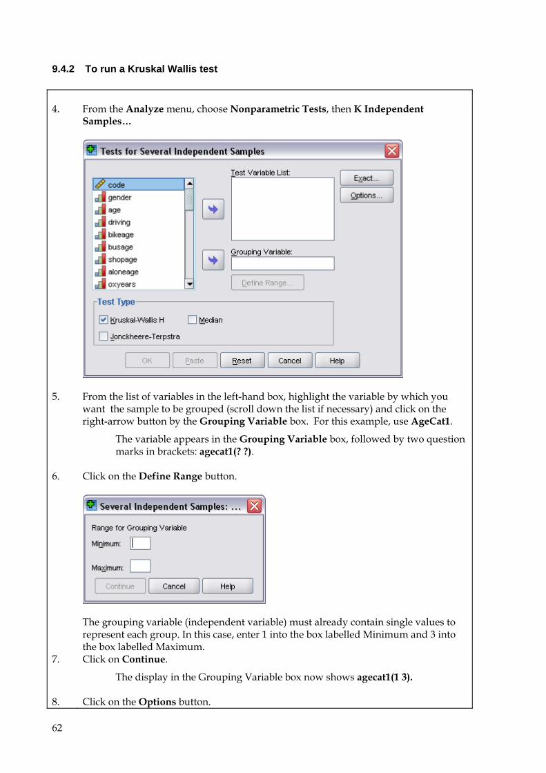
62

9.4.2 To run a Kruskal Wallis test 4. From the Analyze menu, choose Nonparametric Tests, then K Independent

Samples…

5. From the list of variables in the left-hand box, highlight the variable by which you want the sample to be grouped (scroll down the list if necessary) and click on the right-arrow button by the Grouping Variable box. For this example, use AgeCat1.

The variable appears in the Grouping Variable box, followed by two question marks in brackets: agecat1(? ?).

6. Click on the Define Range button.

The grouping variable (independent variable) must already contain single values to represent each group. In this case, enter 1 into the box labelled Minimum and 3 into the box labelled Maximum.

7. Click on Continue.

The display in the Grouping Variable box now shows agecat1(1 3).

8. Click on the Options button.

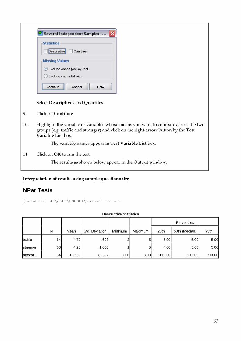
63

Select Descriptives and Quartiles.

9. Click on Continue.

10. Highlight the variable or variables whose means you want to compare across the two groups (e.g. traffic and stranger) and click on the right-arrow button by the Test Variable List box.

The variable names appear in Test Variable List box.

11. Click on OK to run the test.

The results as shown below appear in the Output window.

Interpretation of results using sample questionnaire NPar Tests [DataSet1] U:\data\SOCSCI\spssvalues.sav

Descriptive Statistics

N Mean Std. Deviation Minimum Maximum

Percentiles

25th 50th (Median) 75th

traffic 54 4.70 .603 3 5 5.00 5.00 5.00

stranger 53 4.23 1.050 1 5 4.00 5.00 5.00

agecat1 54 1.9630 .82332 1.00 3.00 1.0000 2.0000 3.0000

64

Kruskal-Wallis Test

Ranks

agecat1 N Mean Rank

traffic 18-19 19 28.24

20-23 18 27.61

24+ 17 26.56

Total 54

stranger 18-19 19 29.66

20-23 18 28.72

24+ 16 21.91

Total 53

Test Statisticsa,b

traffic stranger

Chi-Square .197 3.083

df 2 2

Asymp. Sig. .906 .214

a. Kruskal Wallis Test

b. Grouping Variable: agecat1 Notes: 1. The descriptive statistics table gives the mean and median for each variable but does

not split the dependent variable into the groups defined by the independent variable. Use Analyse – Compare Means – Means to compare the medians and means for each group (the medians could be identical even if there is a significant difference between the groups).

2. For each group, the results show the Number of Cases and Mean Rank. We can see that the mean ranks for traffic are very similar for all three age groups but the oldest age group appears to have a lower mean rank for stranger (21.91) than the others.

3. The test statistic for the Kruskal-Wallis test is called H, but SPSS labels it Chi-Squared. 4. There is no significant effect of age on either ratings of the importance of traffic

danger (H[2]=0.197; n=54; p=.906) nor stranger danger (H[2]=3.083; n=53; p=.214). This result contradicts the result from the Mann-Whitney test which highlights a general trend in statistics. All other things being equal, a complicated design (i.e. with more independent variables or more levels for each independent variable) is less likely to give significant results than a simple model.

65

9.4.3 To run a Wilcoxon test 1. From the Analyze menu, choose Nonparametric Tests, then 2 Related Samples…

2. Click on the Options button.

Select Descriptives and Quartiles.

3. Click on Continue.

4. From the list of variables in the left-hand box, select the variables you wish to compare by clicking on each of them, and then click on the right-arrow. For this example, use traffic and stranger.

The variable pair will appear in the Test Pair(s) List box.

5. Click on OK to run the test.

The results as shown below appear in the Output window.

66

Interpretation of results using sample questionnaire NPar Tests [DataSet1] U:\data\SOCSCI\spssvalues.sav

Descriptive Statistics

N Mean Std. Deviation Minimum Maximum

Percentiles

25th 50th (Median) 75th

traffic 54 4.70 .603 3 5 5.00 5.00 5.00

stranger 53 4.23 1.050 1 5 4.00 5.00 5.00

Wilcoxon Signed Ranks Test

Ranks

N Mean Rank Sum of Ranks

stranger - traffic Negative Ranks 21a 14.86 312.00

Positive Ranks 6b 11.00 66.00

Ties 26c

Total 53

a. stranger < traffic

b. stranger > traffic

c. stranger=traffic

Test Statisticsb

stranger - traffic

Z -3.135a

Asymp. Sig. (2-tailed) .002

a. Based on positive ranks.

b. Wilcoxon Signed Ranks Test

Notes: 1. The Ranks table shows the number of times that the rating for stranger danger is

higher than that for traffic danger, and vice versa, plus the number of ties. 2. The test statistic is called T and is the lower of the two sums of ranks in the Ranks

table. However, you may sometimes see the z value used instead. 3. In the Wilcoxon test, ties are ignored but based on the larger number of negative

ranks than positive ranks the results show than traffic danger was rated as significantly more important than stranger danger (T=66; n=27; p=.002)

4. The direction and size of the effect can be seen by looking at the descriptive statistics.

67

9.4.4 To run a Friedman test 1. From the Analyze menu, choose Nonparametric Tests, then K Related Samples…

2. Click on the Statistics button.

Select Descriptives and Quartiles.

3. Click on Continue.

4. Highlight the variables to be compared (e.g. oxcity, mapread and spatial which are all measured on the same 5 point Likert scale) and click on the right-arrow button by the Test Variables box.

The variable names appear in Test Variables box.

5. Click on OK to run the test.

The results as shown below appear in the Output window.

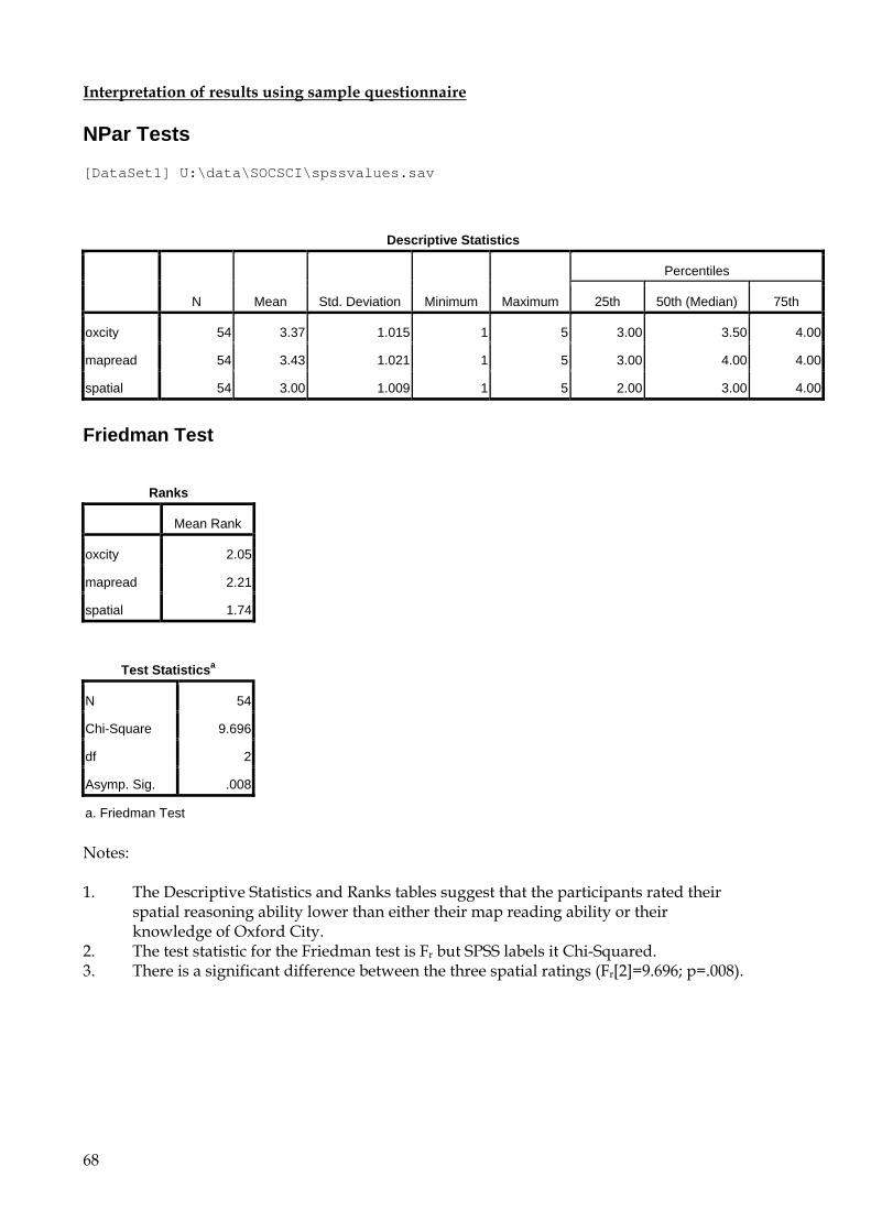
68

Interpretation of results using sample questionnaire NPar Tests [DataSet1] U:\data\SOCSCI\spssvalues.sav

Descriptive Statistics

N Mean Std. Deviation Minimum Maximum

Percentiles

25th 50th (Median) 75th

oxcity 54 3.37 1.015 1 5 3.00 3.50 4.00

mapread 54 3.43 1.021 1 5 3.00 4.00 4.00

spatial 54 3.00 1.009 1 5 2.00 3.00 4.00

Friedman Test

Ranks

Mean Rank

oxcity 2.05

mapread 2.21

spatial 1.74

Test Statisticsa

N 54

Chi-Square 9.696

df 2

Asymp. Sig. .008

a. Friedman Test Notes: 1. The Descriptive Statistics and Ranks tables suggest that the participants rated their

spatial reasoning ability lower than either their map reading ability or their knowledge of Oxford City.

2. The test statistic for the Friedman test is Fr but SPSS labels it Chi-Squared. 3. There is a significant difference between the three spatial ratings (Fr[2]=9.696; p=.008).

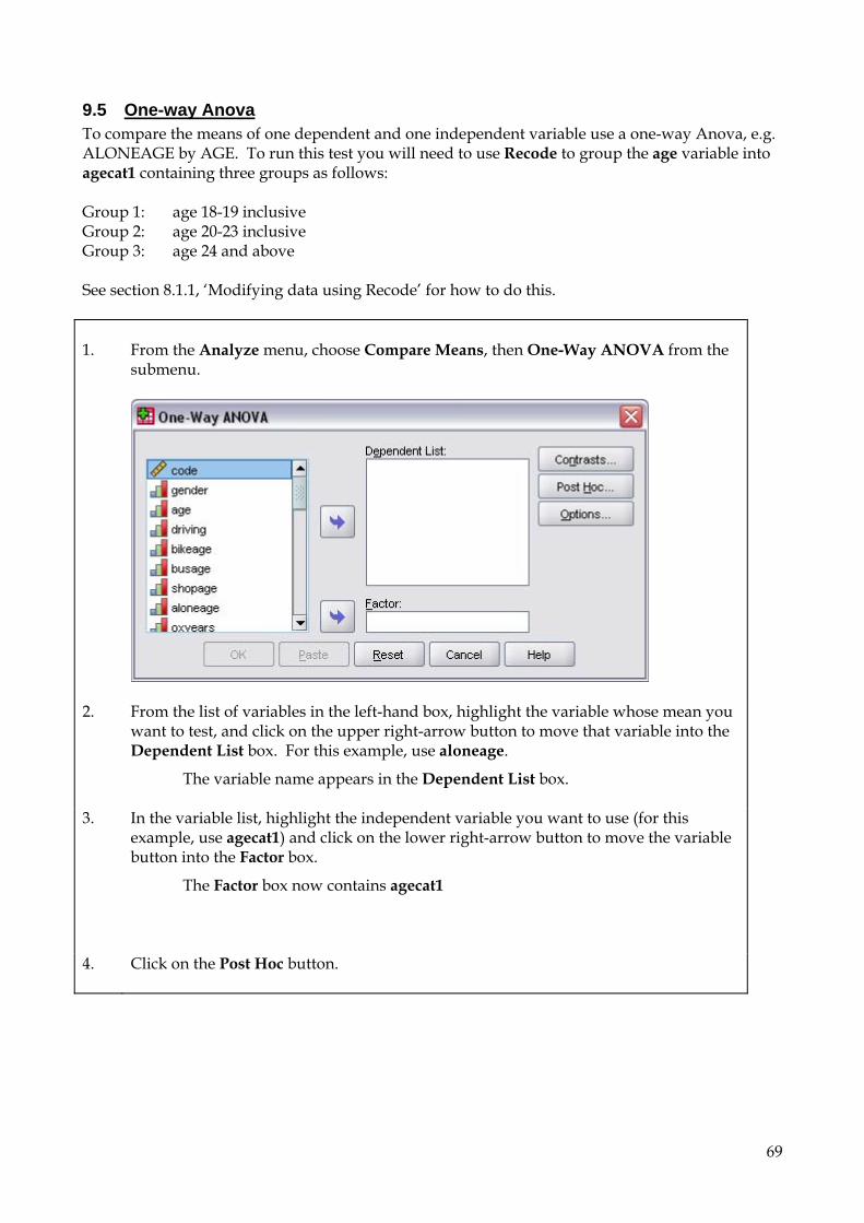
69

9.5 One-way Anova To compare the means of one dependent and one independent variable use a one-way Anova, e.g. ALONEAGE by AGE. To run this test you will need to use Recode to group the age variable into agecat1 containing three groups as follows: Group 1: age 18-19 inclusive Group 2: age 20-23 inclusive Group 3: age 24 and above See section 8.1.1, ‘Modifying data using Recode’ for how to do this. 1. From the Analyze menu, choose Compare Means, then One-Way ANOVA from the

submenu.

2. From the list of variables in the left-hand box, highlight the variable whose mean you want to test, and click on the upper right-arrow button to move that variable into the Dependent List box. For this example, use aloneage.

The variable name appears in the Dependent List box.

3. In the variable list, highlight the independent variable you want to use (for this example, use agecat1) and click on the lower right-arrow button to move the variable button into the Factor box.

The Factor box now contains agecat1

4. Click on the Post Hoc button.

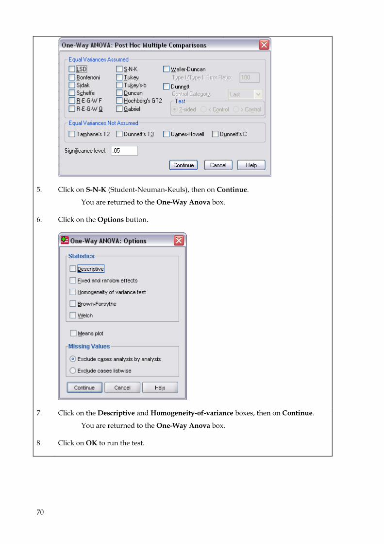
70

5. Click on S-N-K (Student-Neuman-Keuls), then on Continue.

You are returned to the One-Way Anova box.

6. Click on the Options button.

7. Click on the Descriptive and Homogeneity-of-variance boxes, then on Continue.

You are returned to the One-Way Anova box.

8. Click on OK to run the test.

71

Interpretation of results using sample questionnaire A one-way Anova comparing the mean age respondents were first allowed to go out alone, by age (grouped into ages 18-19, 20-23, and 24+) i.e. one dependent variable (aloneage), and one independent variable (agecat1). Oneway [DataSet1] U:\data\SOCSCI\spssvalues.sav

Descriptives

aloneage

N Mean Std. Deviation Std. Error

95% Confidence Interval for

Mean

Minimum Maximum Lower Bound Upper Bound

18-19 19 15.32 1.857 .426 14.42 16.21 12 18

20-23 18 14.72 2.906 .685 13.28 16.17 7 20

24+ 17 12.29 4.552 1.104 9.95 14.63 4 19

Total 54 14.17 3.441 .468 13.23 15.11 4 20

Test of Homogeneity of Variances

aloneage

Levene Statistic df1 df2 Sig.

8.569 2 51 .001

ANOVA

aloneage

Sum of Squares df Mean Square F Sig.

Between Groups 90.254 2 45.127 4.284 .019

Within Groups 537.246 51 10.534

Total 627.500 53

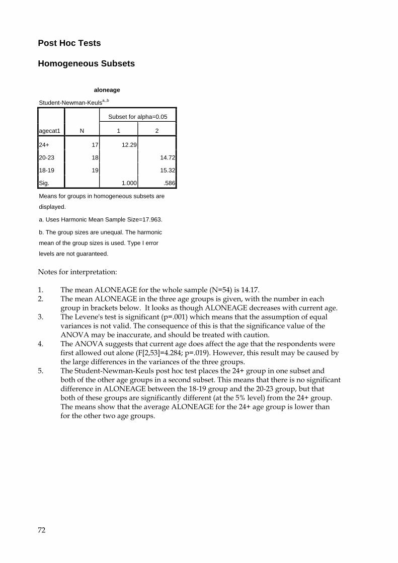
72

Post Hoc Tests Homogeneous Subsets

aloneage

Student-Newman-Keulsa,,b

agecat1 N

Subset for alpha=0.05

1 2

24+ 17 12.29

20-23 18 14.72

18-19 19 15.32

Sig. 1.000 .586

Means for groups in homogeneous subsets are

displayed.

a. Uses Harmonic Mean Sample Size=17.963.

b. The group sizes are unequal. The harmonic

mean of the group sizes is used. Type I error

levels are not guaranteed. Notes for interpretation: 1. The mean ALONEAGE for the whole sample (N=54) is 14.17. 2. The mean ALONEAGE in the three age groups is given, with the number in each

group in brackets below. It looks as though ALONEAGE decreases with current age. 3. The Levene's test is significant (p=.001) which means that the assumption of equal

variances is not valid. The consequence of this is that the significance value of the ANOVA may be inaccurate, and should be treated with caution.

4. The ANOVA suggests that current age does affect the age that the respondents were first allowed out alone (F[2,53]=4.284; p=.019). However, this result may be caused by the large differences in the variances of the three groups.

5. The Student-Newman-Keuls post hoc test places the 24+ group in one subset and both of the other age groups in a second subset. This means that there is no significant difference in ALONEAGE between the 18-19 group and the 20-23 group, but that both of these groups are significantly different (at the 5% level) from the 24+ group. The means show that the average ALONEAGE for the 24+ age group is lower than for the other two age groups.

73

9.6 Two-way Anova To compare the means of one dependent variable on more than one independent variable, use a Two-way Anova, also known as a Simple Factorial Anova or Univariate Anova, e.g. ALONEAGE by AGE and GENDER. It is inappropriate to use agecat1 for this analysis, because there are no males in the 18-19 age group. Instead, a new variable should be created called agecat2 which divides the group into those who are 21 or less and those who are over 21. 1. From the Analyze menu, choose General Linear Model, then Univariate from the

submenu.

2. From the list of variables in the left-hand pane, highlight the variable whose mean you want to test, and click on the uppermost right-arrow button to move that variable into the Dependent variable box. For this example, use aloneage.

The variable name appears in the Dependent variable box.

3. In the variable list, highlight the independent variable you want to use (for this example, use agecat2) and click on the middle right-arrow button to move the variable into the Fixed Factor(s) box.

The Fixed Factor(s) box now contains agecat2

4. In the variable list on the left, choose another independent variable (or Fixed Factor). For this example, use gender. Click on the middle right-arrow button to move it into the Fixed Factor(s) pane.

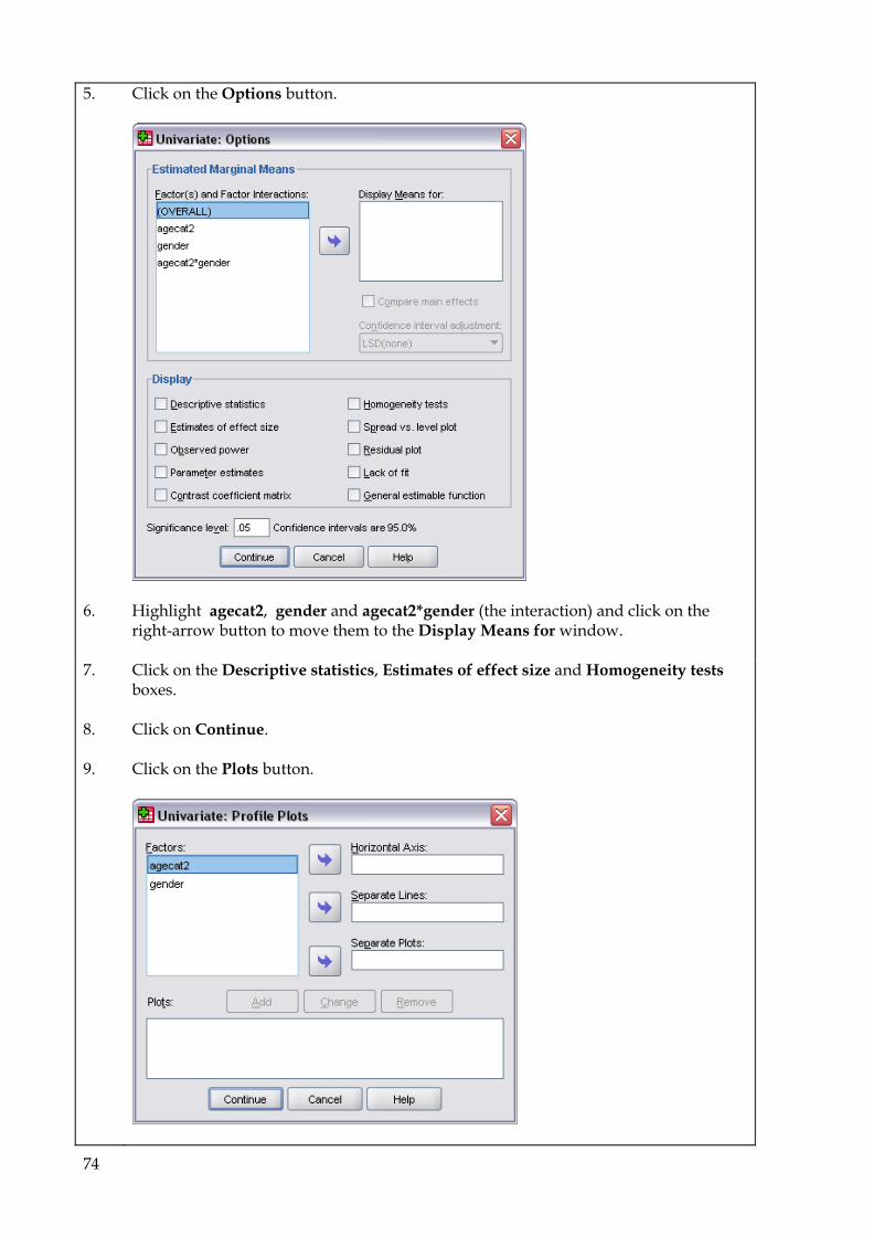
74

5. Click on the Options button.

6. Highlight agecat2, gender and agecat2*gender (the interaction) and click on the right-arrow button to move them to the Display Means for window.

7. Click on the Descriptive statistics, Estimates of effect size and Homogeneity tests boxes.

8. Click on Continue.

9. Click on the Plots button.

75

10. Select agecat2 and push it into the Horizontal Axis box using the top arrow. Select gender and push it into the Separate Lines box using the second arrow. If you put the two independent variables the other way around, then the graph will still be correct but some graphs are easier to interpret than others. Here are a few conventions to help you decide which way is likely to be the easiest to interpret.

• Time should go on the horizontal axis. • The variable with the most categories should go on the horizontal axis. • If you want two graphs which share a common variable, that variable should

go on the horizontal axis. In order to show a three-way interaction (not applicable in this case) the third variable should go into the Separate Plots box.

11. Click on the Add button to add the desired graph into the Plots box.

12. Click on Continue.

13. In this case, both independent variables only have two levels each. If an independent variable has 3 or more levels, click on the Post Hoc button, push the variable(s) with more than two levels into the right hand box and select S-N-K. See Section 9.5 One-Way ANOVA for more details of post hoc tests.

14. Click on OK to run the test.

Example A two-way Anova comparing the mean scores on the aloneage question by agecat2 and gender, i.e. two independent variables (agecat2, gender), and one dependent variable (aloneage). This example requires the age variable to be recoded into two groups (up to 21 and over 21) as above before running the Anova. See section 8.1.1, ‘Modifying data using Recode’ for how to do this. Univariate Analysis of Variance [DataSet1] U:\data\SOCSCI\spssvalues.sav

Between-Subjects Factors

Value Label N

agecat2 1.00 Up to 21 30

2.00 Over 21 24

gender 1 Male 7

2 Female 47

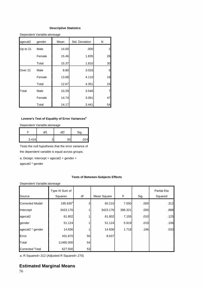
76

Descriptive Statistics

Dependent Variable:aloneage

agecat2 gender Mean Std. Deviation N

Up to 21 Male 14.00 .000 2

Female 15.46 1.835 28

Total 15.37 1.810 30

Over 21 Male 8.80 3.033 5

Female 13.68 4.110 19

Total 12.67 4.351 24

Total Male 10.29 3.546 7

Female 14.74 3.061 47

Total 14.17 3.441 54

Levene's Test of Equality of Error Variancesa

Dependent Variable:aloneage

F df1 df2 Sig.

3.416 3 50 .024

Tests the null hypothesis that the error variance of

the dependent variable is equal across groups.

a. Design: Intercept + agecat2 + gender +

agecat2 * gender

Tests of Between-Subjects Effects

Dependent Variable:aloneage

Source

Type III Sum of

Squares df Mean Square F Sig.

Partial Eta

Squared

Corrected Model 195.630a 3 65.210 7.550 .000 .312

Intercept 3423.176 1 3423.176 396.321 .000 .888

agecat2 61.802 1 61.802 7.155 .010 .125

gender 51.124 1 51.124 5.919 .019 .106

agecat2 * gender 14.836 1 14.836 1.718 .196 .033

Error 431.870 50 8.637

Total 11465.000 54

Corrected Total 627.500 53

a. R Squared=.312 (Adjusted R Squared=.270)

Estimated Marginal Means

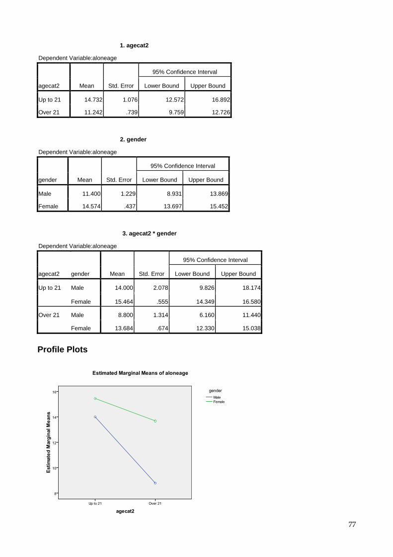
77

1. agecat2

Dependent Variable:aloneage

agecat2 Mean Std. Error

95% Confidence Interval

Lower Bound Upper Bound

Up to 21 14.732 1.076 12.572 16.892

Over 21 11.242 .739 9.759 12.726

2. gender

Dependent Variable:aloneage

gender Mean Std. Error

95% Confidence Interval

Lower Bound Upper Bound

Male 11.400 1.229 8.931 13.869

Female 14.574 .437 13.697 15.452

3. agecat2 * gender

Dependent Variable:aloneage

agecat2 gender Mean Std. Error

95% Confidence Interval

Lower Bound Upper Bound

Up to 21 Male 14.000 2.078 9.826 18.174

Female 15.464 .555 14.349 16.580

Over 21 Male 8.800 1.314 6.160 11.440

Female 13.684 .674 12.330 15.038

Profile Plots

78

Notes: 1. The Levene test is significant (p=.024), so equal variances can not be assumed. This

means that the results of the Anova may be unreliable. However, this is not surprising since there are only 7 males, compared with 47 females in the sample.

2. The analysis suggests that there is a significant difference in perceived aloneage according to age group (F[1,50]=7.16; p=.010). The marginal means show that the average age the younger group were first allowed out alone (14.7) is later than the age the older group were first allowed out alone (11.2).

3. There is also sex difference (F[1,50]=5.92; p=.019). The marginal means show that the average age that males were first allowed out alone (11.4) is earlier than the age that females were first allowed out alone (14.6).

4. There is no interaction between agecat2 and gender on aloneage (F[1,50]=1.72; p=.196). This suggests that the effects of AGE and GENDER are independent and additive.

5. Partial Eta Squared is a standard measure of effect size. ηp2=SSeffect / (SSeffect + SSerror) It has a maximum value of 1. Partial Eta Squared values are not additive, i.e. the sum of the values for all the main effects and interactions could add up to more than 1.

6. By default, SPSS selects the scale on the vertical axis of its graphs to maximize the apparent differences between the points. Therefore, you must look at the significance of the interaction before interpreting the graph. From the graph it looks like the effect of gender on aloneage was greater for the older age group than the younger one. However, since the interaction is neither significant, nor approaching significance (p<.100) then the correct interpretation is that the effect of gender on aloneage was the same for both age groups.

7. To change the scale on the y-axis, the line styles or any other aspects of the graph, double-click on it to open the chart editor and then double-click on the aspect you want to change. This will open the correct dialogue box. N.B. In order to make future graphs appear with lines suitable for back and white printing instead of coloured lines, select the Edit menu, and choose Options. Then select the Charts tag to show the chart options and choose Cycle through patterns and then press the OK button.

8. The Post Hoc option in Univariate will allow you to perform post hoc tests on the main effects, but not the interaction. If you need to compare means for the interaction statistically, it is possible to do this by hand. See Chapter 10, Multiple Comparison in the Analysis of Variance, specifically Duncan’s New Multiple Range Test, in A.L. Edwards, Experimental Design in Psychological research, 1960, Holt, Rinehart and Winston. Alternatively you could collapse your data into a one-way analysis of variance and use the Post Hoc command as specified earlier.

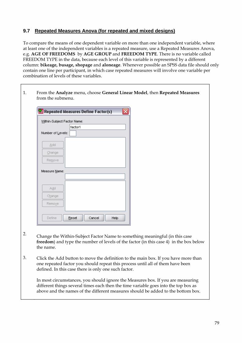
79

9.7 Repeated Measures Anova (for repeated and mixed designs) To compare the means of one dependent variable on more than one independent variable, where at least one of the independent variables is a repeated measure, use a Repeated Measures Anova, e.g. AGE OF FREEDOMS by AGE GROUP and FREEDOM TYPE. There is no variable called FREEDOM TYPE in the data, because each level of this variable is represented by a different column: bikeage, busage, shopage and aloneage. Whenever possible an SPSS data file should only contain one line per participant, in which case repeated measures will involve one variable per combination of levels of these variables. 1. From the Analyze menu, choose General Linear Model, then Repeated Measures

from the submenu.

2. Change the Within-Subject Factor Name to something meaningful (in this case freedom) and type the number of levels of the factor (in this case 4) in the box below the name.

3. Click the Add button to move the definition to the main box. If you have more than one repeated factor you should repeat this process until all of them have been defined. In this case there is only one such factor. In most circumstances, you should ignore the Measures box. If you are measuring different things several times each then the time variable goes into the top box as above and the names of the different measures should be added to the bottom box.

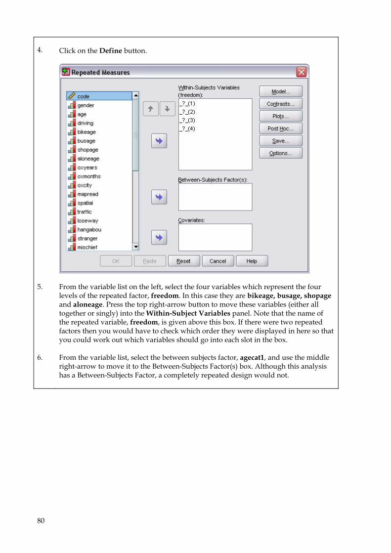
80

4. Click on the Define button.

5. From the variable list on the left, select the four variables which represent the four levels of the repeated factor, freedom. In this case they are bikeage, busage, shopage and aloneage. Press the top right-arrow button to move these variables (either all together or singly) into the Within-Subject Variables panel. Note that the name of the repeated variable, freedom, is given above this box. If there were two repeated factors then you would have to check which order they were displayed in here so that you could work out which variables should go into each slot in the box.

6. From the variable list, select the between subjects factor, agecat1, and use the middle right-arrow to move it to the Between-Subjects Factor(s) box. Although this analysis has a Between-Subjects Factor, a completely repeated design would not.

81

7. Click on the Post Hoc button.

8. Select agecat1 and use the right arrow to move that variable across to the Post-Hoc Tests box. Note that these post-hoc tests are only offered for between subjects factors.

9. Click on S-N-K (Student-Neuman-Keuls), then on Continue.

You are returned to the Repeated Measures dialogue box.

10. Click on the Options button.

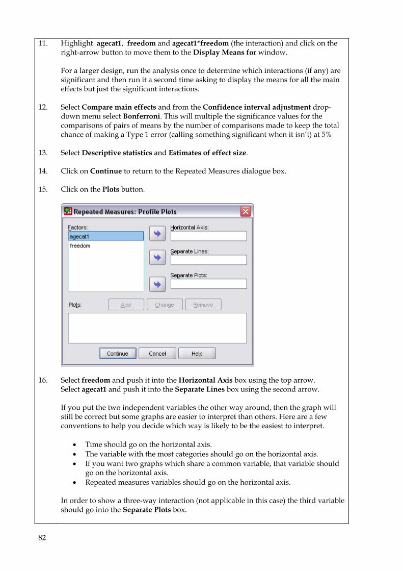
82

11. Highlight agecat1, freedom and agecat1*freedom (the interaction) and click on the right-arrow button to move them to the Display Means for window. For a larger design, run the analysis once to determine which interactions (if any) are significant and then run it a second time asking to display the means for all the main effects but just the significant interactions.

12. Select Compare main effects and from the Confidence interval adjustment drop-down menu select Bonferroni. This will multiple the significance values for the comparisons of pairs of means by the number of comparisons made to keep the total chance of making a Type 1 error (calling something significant when it isn’t) at 5%

13. Select Descriptive statistics and Estimates of effect size.

14. Click on Continue to return to the Repeated Measures dialogue box.

15. Click on the Plots button.

16. Select freedom and push it into the Horizontal Axis box using the top arrow. Select agecat1 and push it into the Separate Lines box using the second arrow. If you put the two independent variables the other way around, then the graph will still be correct but some graphs are easier to interpret than others. Here are a few conventions to help you decide which way is likely to be the easiest to interpret.

• Time should go on the horizontal axis. • The variable with the most categories should go on the horizontal axis. • If you want two graphs which share a common variable, that variable should

go on the horizontal axis. • Repeated measures variables should go on the horizontal axis.

In order to show a three-way interaction (not applicable in this case) the third variable should go into the Separate Plots box.

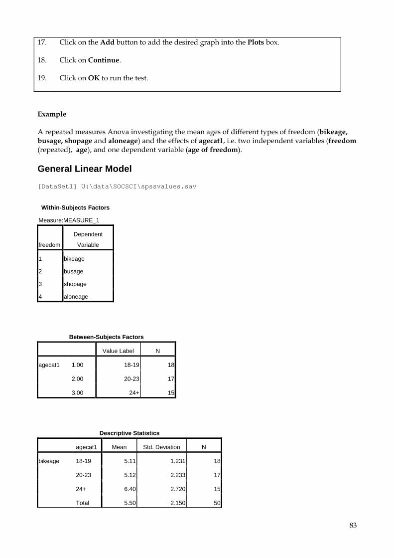
83

17. Click on the Add button to add the desired graph into the Plots box.

18. Click on Continue.

19. Click on OK to run the test.

Example A repeated measures Anova investigating the mean ages of different types of freedom (bikeage, busage, shopage and aloneage) and the effects of agecat1, i.e. two independent variables (freedom (repeated), age), and one dependent variable (age of freedom). General Linear Model [DataSet1] U:\data\SOCSCI\spssvalues.sav

Within-Subjects Factors

Measure:MEASURE_1

freedom

Dependent

Variable

1 bikeage

2 busage

3 shopage

4 aloneage

Between-Subjects Factors

Value Label N

agecat1 1.00 18-19 18

2.00 20-23 17

3.00 24+ 15

Descriptive Statistics

agecat1 Mean Std. Deviation N

bikeage 18-19 5.11 1.231 18

20-23 5.12 2.233 17

24+ 6.40 2.720 15

Total 5.50 2.150 50

84

busage 18-19 11.72 1.809 18

20-23 11.06 1.345 17

24+ 10.73 2.374 15

Total 11.20 1.874 50

shopage 18-19 10.94 2.485 18

20-23 10.71 1.961 17

24+ 10.13 2.264 15

Total 10.62 2.230 50

aloneage 18-19 15.50 1.724 18

20-23 14.65 2.978 17

24+ 12.73 4.284 15

Total 14.38 3.238 50

Multivariate Testsc

Effect Value F Hypothesis df Error df Sig.

Partial Eta

Squared

freedom Pillai's Trace .876 106.431a 3.000 45.000 .000 .876

Wilks' Lambda .124 106.431a 3.000 45.000 .000 .876

Hotelling's Trace 7.095 106.431a 3.000 45.000 .000 .876

Roy's Largest Root 7.095 106.431a 3.000 45.000 .000 .876

freedom * agecat1 Pillai's Trace .212 1.818 6.000 92.000 .104 .106

Wilks' Lambda .791 1.871a 6.000 90.000 .094 .111

Hotelling's Trace .262 1.920 6.000 88.000 .086 .116

Roy's Largest Root .249 3.819b 3.000 46.000 .016 .199

a. Exact statistic

b. The statistic is an upper bound on F that yields a lower bound on the significance level.

c. Design: Intercept + agecat1

Within Subjects Design: freedom

Mauchly's Test of Sphericityb

Measure:MEASURE_1

Within

Subjects

Effect Mauchly's W

Approx. Chi-

Square df Sig.

Epsilona

Greenhouse-

Geisser Huynh-Feldt Lower-bound

freedom .548 27.464 5 .000 .763 .838 .333

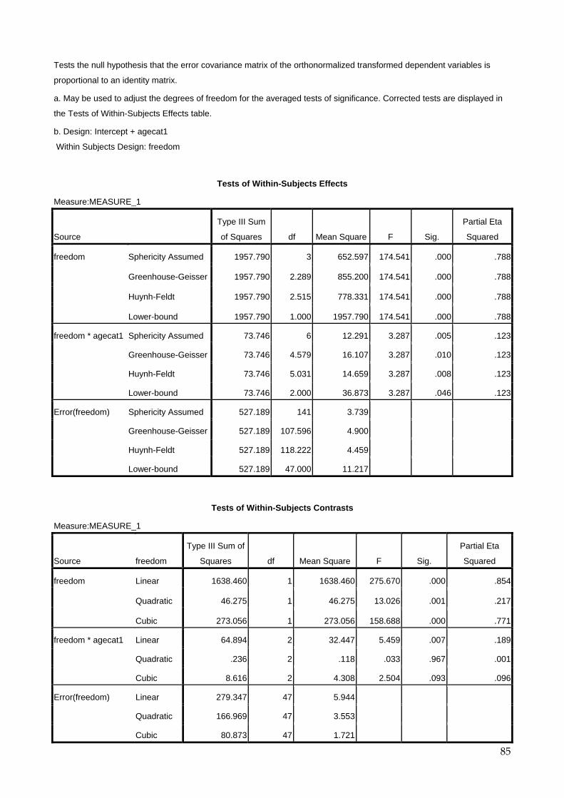
85

Tests the null hypothesis that the error covariance matrix of the orthonormalized transformed dependent variables is

proportional to an identity matrix.

a. May be used to adjust the degrees of freedom for the averaged tests of significance. Corrected tests are displayed in

the Tests of Within-Subjects Effects table.

b. Design: Intercept + agecat1

Within Subjects Design: freedom

Tests of Within-Subjects Effects

Measure:MEASURE_1

Source

Type III Sum

of Squares df Mean Square F Sig.

Partial Eta

Squared

freedom Sphericity Assumed 1957.790 3 652.597 174.541 .000 .788

Greenhouse-Geisser 1957.790 2.289 855.200 174.541 .000 .788

Huynh-Feldt 1957.790 2.515 778.331 174.541 .000 .788

Lower-bound 1957.790 1.000 1957.790 174.541 .000 .788

freedom * agecat1 Sphericity Assumed 73.746 6 12.291 3.287 .005 .123

Greenhouse-Geisser 73.746 4.579 16.107 3.287 .010 .123

Huynh-Feldt 73.746 5.031 14.659 3.287 .008 .123

Lower-bound 73.746 2.000 36.873 3.287 .046 .123

Error(freedom) Sphericity Assumed 527.189 141 3.739

Greenhouse-Geisser 527.189 107.596 4.900

Huynh-Feldt 527.189 118.222 4.459

Lower-bound 527.189 47.000 11.217

Tests of Within-Subjects Contrasts

Measure:MEASURE_1

Source freedom

Type III Sum of

Squares df Mean Square F Sig.

Partial Eta

Squared

freedom Linear 1638.460 1 1638.460 275.670 .000 .854

Quadratic 46.275 1 46.275 13.026 .001 .217

Cubic 273.056 1 273.056 158.688 .000 .771

freedom * agecat1 Linear 64.894 2 32.447 5.459 .007 .189

Quadratic .236 2 .118 .033 .967 .001

Cubic 8.616 2 4.308 2.504 .093 .096

Error(freedom) Linear 279.347 47 5.944

Quadratic 166.969 47 3.553

Cubic 80.873 47 1.721

86

Tests of Between-Subjects Effects

Measure:MEASURE_1

Transformed Variable:Average

Source

Type III Sum of

Squares df Mean Square F Sig.

Partial Eta

Squared

Intercept 21509.528 1 21509.528 1896.849 .000 .976

agecat1 22.163 2 11.082 .977 .384 .040

Error 532.962 47 11.340

Estimated Marginal Means 1. agecat1

Estimates

Measure:MEASURE_1

agecat1 Mean Std. Error

95% Confidence Interval

Lower Bound Upper Bound

18-19 10.819 .397 10.021 11.618

20-23 10.382 .408 9.561 11.204

24+ 10.000 .435 9.125 10.875

Pairwise Comparisons

Measure:MEASURE_1

(I)

agecat1

(J)

agecat1

Mean Difference

(I-J) Std. Error Sig.a

95% Confidence Interval for

Differencea

Lower Bound Upper Bound

18-19 20-23 .437 .569 1.000 -.977 1.851

24+ .819 .589 .511 -.642 2.281

20-23 18-19 -.437 .569 1.000 -1.851 .977

24+ .382 .596 1.000 -1.098 1.863

24+ 18-19 -.819 .589 .511 -2.281 .642

20-23 -.382 .596 1.000 -1.863 1.098

Based on estimated marginal means

a. Adjustment for multiple comparisons: Bonferroni.

Univariate Tests

87

Measure:MEASURE_1

Sum of Squares df Mean Square F Sig.

Partial Eta

Squared

Contrast 5.541 2 2.770 .977 .384 .040

Error 133.240 47 2.835

The F tests the effect of agecat1. This test is based on the linearly independent pairwise comparisons among

the estimated marginal means.

2. freedom

Estimates

Measure:MEASURE_1

freedom Mean Std. Error

95% Confidence Interval

Lower Bound Upper Bound

1 5.543 .299 4.941 6.145

2 11.171 .265 10.639 11.704

3 10.595 .319 9.952 11.237

4 14.293 .439 13.411 15.176

Pairwise Comparisons

Measure:MEASURE_1

(I)

freedom

(J)

freedom

Mean Difference

(I-J) Std. Error Sig.a

95% Confidence Interval for

Differencea

Lower Bound Upper Bound

1 2 -5.629* .363 .000 -6.630 -4.628

3 -5.052* .403 .000 -6.162 -3.941

4 -8.751* .505 .000 -10.142 -7.360

2 1 5.629* .363 .000 4.628 6.630

3 .577 .231 .096 -.059 1.213

4 -3.122* .377 .000 -4.159 -2.085

3 1 5.052* .403 .000 3.941 6.162

2 -.577 .231 .096 -1.213 .059

4 -3.699* .397 .000 -4.794 -2.604

4 1 8.751* .505 .000 7.360 10.142

2 3.122* .377 .000 2.085 4.159

3 3.699* .397 .000 2.604 4.794

Based on estimated marginal means

88

*. The mean difference is significant at the .05 level.

a. Adjustment for multiple comparisons: Bonferroni.

Multivariate Tests

Value F Hypothesis df Error df Sig.

Partial Eta

Squared

Pillai's trace .876 106.431a 3.000 45.000 .000 .876

Wilks' lambda .124 106.431a 3.000 45.000 .000 .876

Hotelling's trace 7.095 106.431a 3.000 45.000 .000 .876

Roy's largest root 7.095 106.431a 3.000 45.000 .000 .876

Each F tests the multivariate effect of freedom. These tests are based on the linearly independent pairwise

comparisons among the estimated marginal means.

a. Exact statistic

3. agecat1 * freedom

Measure:MEASURE_1

agecat1 freedom Mean Std. Error

95% Confidence Interval

Lower Bound Upper Bound

18-19 1 5.111 .497 4.111 6.111

2 11.722 .440 10.838 12.607

3 10.944 .531 9.877 12.012

4 15.500 .729 14.034 16.966

20-23 1 5.118 .512 4.088 6.147

2 11.059 .452 10.149 11.969

3 10.706 .546 9.607 11.804

4 14.647 .750 13.138 16.156

24+ 1 6.400 .545 5.304 7.496

2 10.733 .482 9.765 11.702

3 10.133 .581 8.964 11.303

4 12.733 .798 11.127 14.339

Post Hoc Tests agecat1 Homogeneous Subsets

MEASURE_1

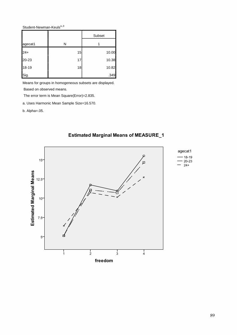
89

Student-Newman-Keulsa,,b

agecat1 N

Subset

1

24+ 15 10.00

20-23 17 10.38

18-19 18 10.82

Sig. .349

Means for groups in homogeneous subsets are displayed.

Based on observed means.

The error term is Mean Square(Error)=2.835.

a. Uses Harmonic Mean Sample Size=16.570.

b. Alpha=.05.

90

Notes: 1. The first step is to look at Mauchly's Test of Sphericity. This is similar to Levene's test

in the previous analysis. If Mauchly's test is not significant, then use the 'Sphericity Assumed rows in the 'Tests of Within Subjects Effects' table. If Mauchly's test is significant, then use the Pillai's Trace rows in the Multivariate tests, unless you are sure that the dependent variables are normally distributed in which case you can use the Greenhouse-Geisser rows on the 'Tests of Within Subjects Effects' table. In this case Mauchly's test is significant and some of the distributions look to be bimodal (twin peaks) so I shall use Pillai's trace. N.B. If all of your repeated variables only have two levels the Mauchly test is not applicable and you should ignore the Mutivariate tests and use the Sphericity Assumed rows in the 'Tests of Within Subjects Effects' table (which will be identical to the other rows in the same table).

2. There is a highly significant effect of Freedom Type on Freedom Age (Pillai's F[3,45]=106.43; p<.001). The Partial Eta Squared for this effect is 0.876 which is very large. Most of the variation in age of freedom is due to the type of freedom.

3. The interaction between Freedom Type and Age Category is not significant (Pillai's F[6,92]=1.82; p=.106). If the Greenhouse-Geisser or Sphericity assumed rows had been used instead, this interaction would have been found to be significant.

4. The Tests of Between Subject Effects table shows that there is no main effect of age group on the overall freedom ages. (F[2,47]=0.977; p=.384)

5. Ignore the Tests of Within Subject Contrasts table. 6. For each of the main effects there is a table of Pairwise Comparisons as well as the

estimates table. Each row of the comparisons table shows the mean difference between the level in the first column (I) and the level in the second column (J). For the type of freedom, all types are highly significantly different from each other apart from 2 and 3 which correspond to busage and shopage.

9.8 Multiple Regression

9.8.1 Introduction Analysis of variance is designed to be used to investigate the effects of categorical independent variables on an interval dependent variable. If one or more of the independent variables are interval then there are three options available: 1. Split the interval variable(s) into a small number of categories (e.g. usually 2 or 3 and no more

than 5). This recoded variable can now be treated in the analysis as if it were categorical. However, this loses information that has been collected about the variable. Also, ANOVA treats the categories within each variable as unordered, which loses even more information about the variable and reduces the levels of significance of any linear effects present. However, if there are non-linear effects then these may be missed by the other options.

2. Use the interval variable as a covariate in an analysis of variance. This does not lose information but is intended to be used not to investigate the interval variable but to remove their effects before looking at the effects of the categorical variables.

3. Use linear regression. This attempts to predict the observed values of the dependent variable by finding the best linear combination of the chosen independent variables.

The key features of Multiple Linear Regression are as follows:

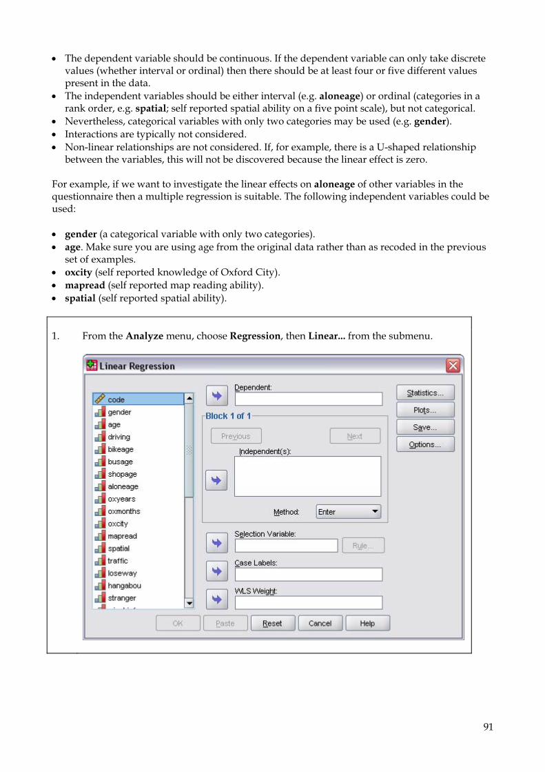
91

• The dependent variable should be continuous. If the dependent variable can only take discrete values (whether interval or ordinal) then there should be at least four or five different values present in the data.

• The independent variables should be either interval (e.g. aloneage) or ordinal (categories in a rank order, e.g. spatial; self reported spatial ability on a five point scale), but not categorical.

• Nevertheless, categorical variables with only two categories may be used (e.g. gender). • Interactions are typically not considered. • Non-linear relationships are not considered. If, for example, there is a U-shaped relationship

between the variables, this will not be discovered because the linear effect is zero. For example, if we want to investigate the linear effects on aloneage of other variables in the questionnaire then a multiple regression is suitable. The following independent variables could be used: • gender (a categorical variable with only two categories). • age. Make sure you are using age from the original data rather than as recoded in the previous

set of examples. • oxcity (self reported knowledge of Oxford City). • mapread (self reported map reading ability). • spatial (self reported spatial ability). 1. From the Analyze menu, choose Regression, then Linear... from the submenu.

92

2. From the list of variables in the left-hand pane, highlight the variable that you want to be able to predict, and click on the uppermost right-arrow button to move that variable into the Dependent box. For this example, use aloneage.

The variable name appears in the Dependent box.

3. In the variable list, highlight the independent variables you want to use (for this example, use gender, age, oxcity, mapread, and spatial) and click on the middle right-arrow button to move the variables into the Independent(s) box.

The Independent(s) box now contains gender, age, oxcity, mapread, and spatial.

4. Click on the small down-arrow to the right of the Method box to display the list of

available regression methods.

5. Select the Enter method (which is the default).

This will force all the chosen independent variables into the regression analysis. See 9.8.3 below for a discussion of the different methods.

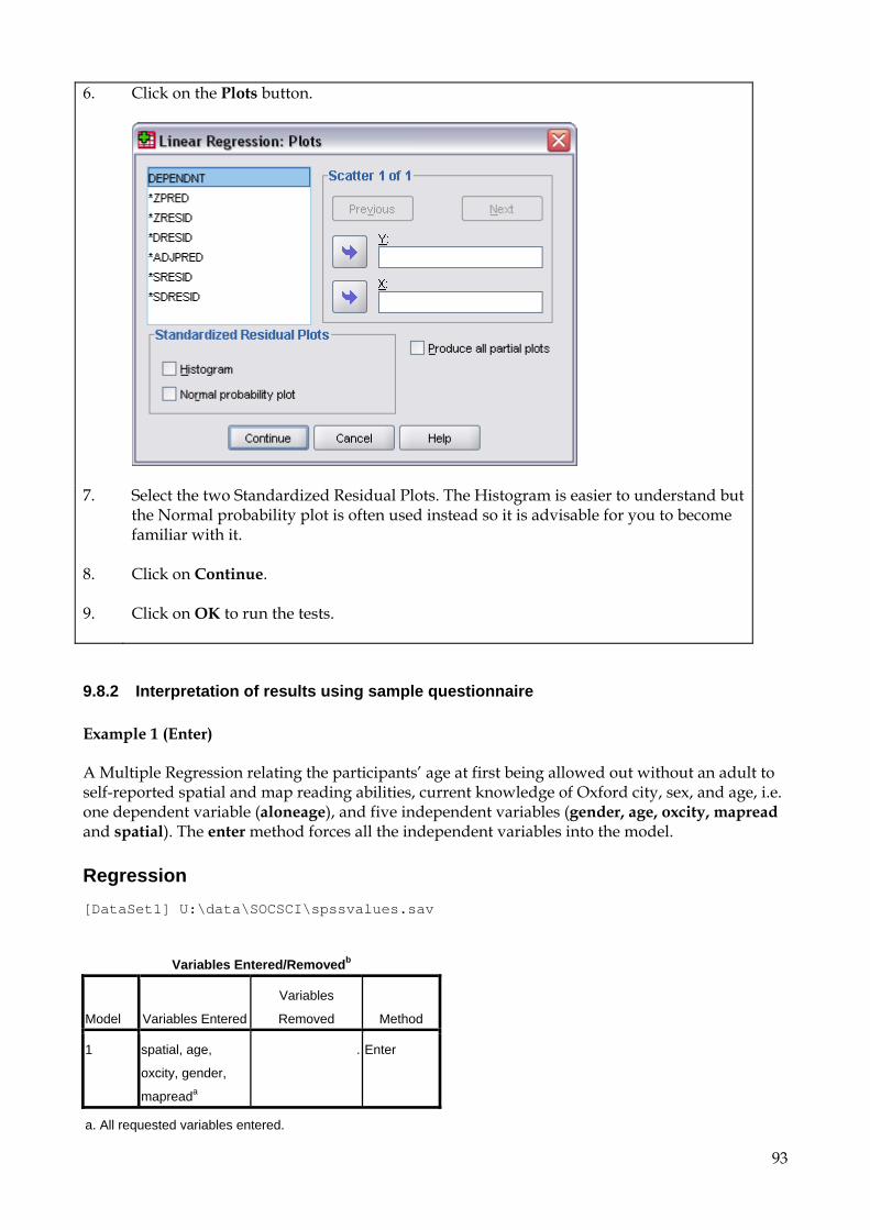
93

6. Click on the Plots button.

7. Select the two Standardized Residual Plots. The Histogram is easier to understand but the Normal probability plot is often used instead so it is advisable for you to become familiar with it.

8. Click on Continue.

9. Click on OK to run the tests.

9.8.2 Interpretation of results using sample questionnaire Example 1 (Enter) A Multiple Regression relating the participants’ age at first being allowed out without an adult to self-reported spatial and map reading abilities, current knowledge of Oxford city, sex, and age, i.e. one dependent variable (aloneage), and five independent variables (gender, age, oxcity, mapread and spatial). The enter method forces all the independent variables into the model. Regression [DataSet1] U:\data\SOCSCI\spssvalues.sav

Variables Entered/Removedb

Model Variables Entered

Variables

Removed Method

1 spatial, age,

oxcity, gender,

mapreada

. Enter

a. All requested variables entered.

94

Variables Entered/Removedb

Model Variables Entered

Variables

Removed Method

1 spatial, age,

oxcity, gender,

mapreada

. Enter

a. All requested variables entered.

b. Dependent Variable: aloneage

Model Summaryb

Model R R Square

Adjusted R

Square

Std. Error of the

Estimate

1 .702a .493 .440 2.575

a. Predictors: (Constant), spatial, age, oxcity, gender, mapread

b. Dependent Variable: aloneage

ANOVAb

Model Sum of Squares df Mean Square F Sig.

1 Regression 309.128 5 61.826 9.321 .000a

Residual 318.372 48 6.633

Total 627.500 53

a. Predictors: (Constant), spatial, age, oxcity, gender, mapread

b. Dependent Variable: aloneage

Coefficientsa

Model

Unstandardized Coefficients

Standardized

Coefficients

t Sig. B Std. Error Beta

1 (Constant) 11.466 3.260 3.517 .001

gender 4.656 1.167 .459 3.990 .000

age -.242 .047 -.572 -5.174 .000

oxcity -.379 .389 -.112 -.974 .335

mapread .181 .467 .054 .387 .700

spatial .175 .509 .051 .344 .732

a. Dependent Variable: aloneage

Residuals Statisticsa

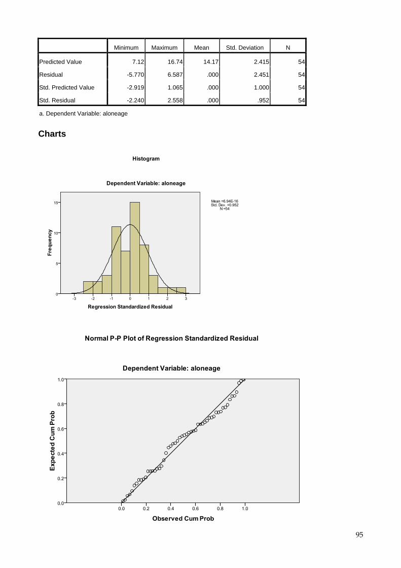
95

Minimum Maximum Mean Std. Deviation N

Predicted Value 7.12 16.74 14.17 2.415 54

Residual -5.770 6.587 .000 2.451 54

Std. Predicted Value -2.919 1.065 .000 1.000 54

Std. Residual -2.240 2.558 .000 .952 54

a. Dependent Variable: aloneage

Charts

96

Notes: 1. R2 in the Model Summary is the proportion of the variance of aloneage explained by

the model (i.e. 49%). The adjusted R2 also takes into account the number of variables in the model so is a better comparison for models of different sizes, but is an index value rather than a proportion so should not normally be used.

2. The ANOVA shows that the model is a highly significant predictor of aloneage (F[5,48]=9.32; p<.001). However, this is not particularly useful since the purpose of the regression is usually to determine which of the independent variables are significant rather than simply assessing the model as a whole.

3. Gender is significantly related to aloneage (t[48]=3.99; p<.001). Since B, Beta and t are all positive, the result shows that females are allowed out alone at a later age on average (high gender corresponds to high aloneage).

4. Age is significantly related to aloneage (t[48]=-5.17; p<.001). Since B, Beta and t are all negative, the result shows that older respondents were allowed out alone at an earlier age on average (high age corresponds to low aloneage).

5. None of the three self assessed abilities are related to aloneage. 6. One of the assumptions of linear regression is that the residuals are normally

distributed. This can be assessed by looking at either of the two charts. The P-P plot straightens the normal curve, turning it into the line y=x, which makes it easier to see where the distribution of the observed residuals deviates from the assumed normal distribution. In this case the distribution is fairly close to being normal.

In this regression, only two out of the five independent variables entered into the model are significantly related to aloneage. Sometimes this can suggest that the model contains too many variables and either fewer variables should be chosen or a different method should be used. If the model contains variables which have no relationship with aloneage or are correlated with other variables in the model then significance of all the variables in the model may be reduced Example 2 (Stepwise) A Multiple Regression relating the respondents’ age of first being allowed out alone, to gender, age, sex, self reported knowledge of Oxford City, self reported map reading ability and self reported spatial ability, i.e. one dependent variable (aloneage), and five independent variables (gender, age, oxcity, mapread and spatial). The stepwise method starts with an empty model and adds one variable at a time in a stepwise fashion until none of the remaining variables will significantly improve the model. It also checks the variables in the equation to see whether any variable should be removed.

Regression [DataSet1] U:\data\SOCSCI\spssvalues.sav

Variables Entered/Removeda

Model

Variables

Entered

Variables

Removed Method

1 age . Stepwise (Criteria: Probability-of-F-to-enter <= .050,

Probability-of-F-to-remove >= .100).

2 gender . Stepwise (Criteria: Probability-of-F-to-enter <= .050,

Probability-of-F-to-remove >= .100).

a. Dependent Variable: aloneage

97

Model Summaryc

Model R R Square

Adjusted R

Square

Std. Error of the

Estimate

1 .538a .290 .276 2.927

2 .693b .480 .460 2.529

a. Predictors: (Constant), age

b. Predictors: (Constant), age, gender

c. Dependent Variable: aloneage

ANOVAc

Model Sum of Squares df Mean Square F Sig.

1 Regression 181.864 1 181.864 21.221 .000a

Residual 445.636 52 8.570

Total 627.500 53

2 Regression 301.393 2 150.697 23.568 .000b

Residual 326.107 51 6.394

Total 627.500 53

a. Predictors: (Constant), age

b. Predictors: (Constant), age, gender

c. Dependent Variable: aloneage

Coefficientsa

Model

Unstandardized Coefficients

Standardized

Coefficients

t Sig. B Std. Error Beta

1 (Constant) 19.695 1.265 15.575 .000

age -.227 .049 -.538 -4.607 .000

2 (Constant) 11.386 2.211 5.151 .000

age -.226 .043 -.536 -5.309 .000

gender 4.429 1.024 .436 4.324 .000

a. Dependent Variable: aloneage

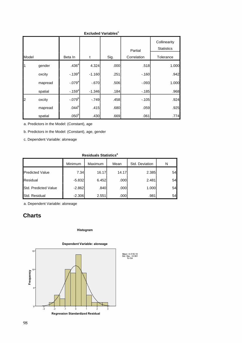
98

Excluded Variablesc

Model Beta In t Sig.

Partial

Correlation

Collinearity

Statistics

Tolerance

1 gender .436a 4.324 .000 .518 1.000

oxcity -.139a -1.160 .251 -.160 .942

mapread -.079a -.670 .506 -.093 1.000

spatial -.159a -1.346 .184 -.185 .968

2 oxcity -.079b -.749 .458 -.105 .924

mapread .044b .415 .680 .059 .925

spatial .050b .430 .669 .061 .774

a. Predictors in the Model: (Constant), age

b. Predictors in the Model: (Constant), age, gender

c. Dependent Variable: aloneage

Residuals Statisticsa

Minimum Maximum Mean Std. Deviation N

Predicted Value 7.34 16.17 14.17 2.385 54

Residual -5.832 6.452 .000 2.481 54

Std. Predicted Value -2.862 .840 .000 1.000 54

Std. Residual -2.306 2.551 .000 .981 54

a. Dependent Variable: aloneage Charts

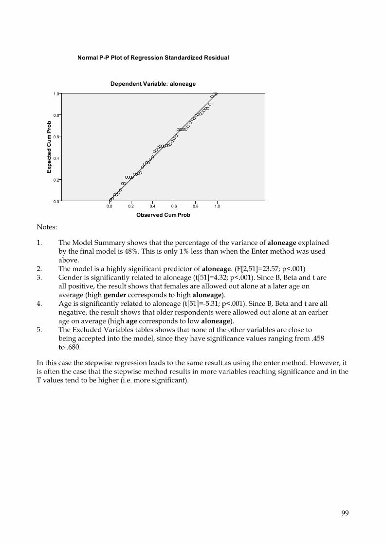
99

Notes: 1. The Model Summary shows that the percentage of the variance of aloneage explained

by the final model is 48%. This is only 1% less than when the Enter method was used above.

2. The model is a highly significant predictor of aloneage. (F[2,51]=23.57; p<.001) 3. Gender is significantly related to aloneage (t[51]=4.32; p<.001). Since B, Beta and t are

all positive, the result shows that females are allowed out alone at a later age on average (high gender corresponds to high aloneage).

4. Age is significantly related to aloneage (t[51]=-5.31; p<.001). Since B, Beta and t are all negative, the result shows that older respondents were allowed out alone at an earlier age on average (high age corresponds to low aloneage).

5. The Excluded Variables tables shows that none of the other variables are close to being accepted into the model, since they have significance values ranging from .458 to .680.

In this case the stepwise regression leads to the same result as using the enter method. However, it is often the case that the stepwise method results in more variables reaching significance and in the T values tend to be higher (i.e. more significant).

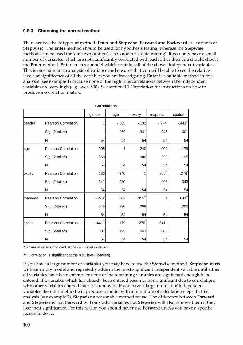
100

9.8.3 Choosing the correct method There are two basic types of method: Enter and Stepwise (Forward and Backward are variants of Stepwise). The Enter method should be used for hypothesis testing, whereas the Stepwise methods can be used for ‘data exploration’, also known as ‘data mining’. If you only have a small number of variables which are not significantly correlated with each other then you should choose the Enter method. Enter creates a model which contains all of the chosen independent variables. This is most similar to analysis of variance and ensures that you will be able to see the relative levels of significance of all the variables you are investigating. Enter is a suitable method in this analysis (see example 1) because none of the high intercorrelations between the independent variables are very high (e.g. over .800). See section 9.1 Correlation for instructions on how to produce a correlation matrix.

Correlations

gender age oxcity mapread spatial

gender Pearson Correlation 1 -.005 -.132 -.274* -.441**

Sig. (2-tailed) .969 .341 .045 .001

N 54 54 54 54 54

age Pearson Correlation -.005 1 -.240 .002 .179

Sig. (2-tailed) .969 .080 .990 .195

N 54 54 54 54 54

oxcity Pearson Correlation -.132 -.240 1 .355** .276*

Sig. (2-tailed) .341 .080 .008 .043

N 54 54 54 54 54

mapread Pearson Correlation -.274* .002 .355** 1 .641**

Sig. (2-tailed) .045 .990 .008 .000

N 54 54 54 54 54

spatial Pearson Correlation -.441** .179 .276* .641** 1

Sig. (2-tailed) .001 .195 .043 .000

N 54 54 54 54 54

*. Correlation is significant at the 0.05 level (2-tailed).

**. Correlation is significant at the 0.01 level (2-tailed).

If you have a large number of variables you may have to use the Stepwise method. Stepwise starts with an empty model and repeatedly adds in the most significant independent variable until either all variables have been entered or none of the remaining variables are significant enough to be entered. If a variable which has already been entered becomes non significant due to correlations with other variables entered later it is removed. If you have a large number of independent variables then this method will produce a model with a minimum of calculation steps. In this analysis (see example 2), Stepwise a reasonable method to use. The difference between Forward and Stepwise is that Forward will only add variables but Stepwise will also remove them if they lose their significance. For this reason you should never use Forward unless you have a specific reason to do so.

101

If you do not have too many variables you can use the Backward method. Backward starts by entering all the independent variables and then repeatedly removes the least significant variable until either no variables are left in the model or all the remaining variables are significant. In this analysis (see example 3), Backward produces the best model out of all three methods, both in terms of the proportion of variance explained (adjusted R square) and the F-ratio for the model. There is often little to chose between Stepwise and Backward. If you use the default cut-off points for entering and removing variables (p=.05 and p=.10 respectively) then variables found between these two points will not be entered using Stepwise but will not be removed using Backward. N.B. Using any of the three Stepwise methods will greatly increase the chance of a Type I error. For this reason they should be used to help generate models for future testing rather than be used to test hypotheses themselves. If you are able to choose the independent variables you wish the place in the model on theoretical grounds then you can use the Enter method and be confident in the significance of your results.

9.9 Factor Analysis

9.9.1 Introduction One of the differences between a questionnaire and an experiment is the number of dependent variables. Often in an experiment there are only one or two final measures, e.g. score and reaction time. However, a questionnaire which only asked one or two questions would be unusual indeed. This presents the a problem when it comes to the statistical analysis. For example on the second page of the Travel questionnaire there are 18 attitude questions. In order to use these variables as dependent there are three methods of proceeding: 1. Analyse each question separately. The problem with this method is that it is both inefficient,

and leads to an increase in Type I errors (claiming a significant finding when there is in fact no effect). This method should be avoided wherever possible.

2. Add together subsets of questions and then analyse these subtotals instead. Although this reduces the chance of Type I errors, it should only be used when it is clear which questions should be grouped together. Reliability analysis (see Section 9.9) can be used to see whether a set of questions can be grouped, but it does cannot simply tell you which subsets to use.

3. Perform a factor analysis to reduce the set of questions to a much smaller number if factors. The choice of factors is made by the computer, leaving you to interpret its decisions. Since this method is the one that is appropriate for most questionnaires, it will be described here.

Factor analysis looks at the correlation matrix of a set of variables and tries to explain as much of the variation present in the data using as few degrees of freedom as possible. Each factor is a linear combination of all of the questions, but will be more closely related to some variables than others. When it comes to interpreting the meaning of a factor, variables which contribute only a very small amount are ignored. A factor analysis should be performed in two stages. The only purpose of the first stage is to find out how many factors should be used in the second stage.

102

9.9.2 How many factors? In this example the 18 attitude questions on page 2 of the Travel questionnaire will be used. 1. From the Analyze menu, choose Dimension Reduction, then Factor... from the

submenu.

2. From the list of variables in the left-hand pane, highlight the variables for the factor analysis., and click on the uppermost right-arrow button to move that variable into the Variables box. For this example, use traffic, loseway, hangabou, stranger, mischief, bully, childwan, enjoy, teachers, parents, work, morechil, pubtimes, pubprice, cyclesaf, toofar, school, donethin.

The variable names appears in the Variables box.

3. Click on the Extraction button. This will open the Extraction dialogue box.

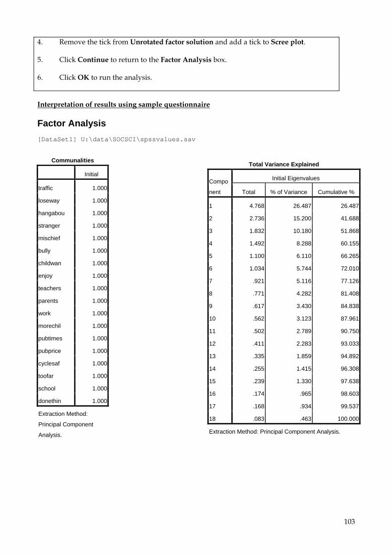
103

4. Remove the tick from Unrotated factor solution and add a tick to Scree plot.

5. Click Continue to return to the Factor Analysis box.

6. Click OK to run the analysis.

Interpretation of results using sample questionnaire Factor Analysis [DataSet1] U:\data\SOCSCI\spssvalues.sav

Communalities

Initial

traffic 1.000

loseway 1.000

hangabou 1.000

stranger 1.000

mischief 1.000

bully 1.000

childwan 1.000

enjoy 1.000

teachers 1.000

parents 1.000

work 1.000

morechil 1.000

pubtimes 1.000

pubprice 1.000

cyclesaf 1.000

toofar 1.000

school 1.000

donethin 1.000

Extraction Method:

Principal Component

Analysis.

Total Variance Explained

Compo

nent

Initial Eigenvalues

Total % of Variance Cumulative %

1 4.768 26.487 26.487

2 2.736 15.200 41.688

3 1.832 10.180 51.868

4 1.492 8.288 60.155

5 1.100 6.110 66.265

6 1.034 5.744 72.010

7 .921 5.116 77.126

8 .771 4.282 81.408

9 .617 3.430 84.838

10 .562 3.123 87.961

11 .502 2.789 90.750

12 .411 2.283 93.033

13 .335 1.859 94.892

14 .255 1.415 96.308

15 .239 1.330 97.638

16 .174 .965 98.603

17 .168 .934 99.537

18 .083 .463 100.000

Extraction Method: Principal Component Analysis.

104

Component Matrixa

a. 6 components

extracted. Notes: 1. The communalities table simply shows which variables have been included in the

factor analysis. 2. The Total Variances Explained table lists 18 components in decreasing order of

importance. For each component the eigenvalue is given, along with the variance explained by that component and the total variance explained by a model using that many factors. N.B. Component 1 is not Variable 1. Every component is a linear combination using larger or smaller 'bits' of all the variables.

3. The eigenvalues can be thought of as indicating how many times better than chance a particular component is at explaining the variation in the data. For example, component 3 has an eigenvalue of 1.832, so that component is nearly twice as good as chance. Component 3 explains just over 10% of the variance by itself, and together with components 1 and 2, a 3 factor solution would explain just over 50%. Any component with an eigenvalue of less than 1 is worse than chance and should not be used in a final solution

4. The Scree Plot gives a more visual display of the eigenvalues. In order to decide how many factors(components) should be used in the second stage of the factor analysis, start at the right hand end of the scree plot and run your eyes along the line, looking for the first discontinuity (bigger vertical gap) above an eigenvalue of 1.

105

In this case there is a discontinuity between components 4 and 5. Although there is also a discontinuity between components 2 & 3, the one between 4 & 5 is the first one above an eigenvalue of 1 when looking from the right hand end. This means that the factor analysis should probably use a 4 factor solution.

9.9.3 The Main Factor Analysis 1. From the Analyze menu, choose Dimension Reduction, then Factor... from the

submenu.

The Factor Analysis dialogue box appears with the same variables as before. The variable list should not be changed.

2. Click on the Extraction button.

106

3. Remove the tick from Scree plot. There is no point producing a second scree plot since it will be identical to the first one.

4. Click on Fixed number of factors and then enter the number of factors you are going to extract into the box to the right. In this case that number is 4.

If the number of factors is only 1, then place a tick in Unrotated factor solution.

5. Click on Continue to return to the main Factor Analysis box.

6. Click on the Rotation button.

7. If you are extracting at least 2 factors, click on Varimax rotation. You do not need to understand the mechanics of factor rotation, but the basic idea is that this should make the factors easier to interpret (by making large correlations larger and small correlations smaller so that each variable is correlates with one factor much more than with the others).

8. Click on Continue to return to the main Factor Analysis box.

9. Click on the Scores button. This will open the Scores dialogue box.

10. Click on Save as variables. This will create a new variable for each factor in the analysis.

107

11. Click on Continue to return to the main Factor Analysis box.

12. Click on the Options button.

13. Click on Sorted by size and Suppress absolute values less than. These options will simplify the interpretation of the factors. N.B. If you have significant amounts of missing data and need to select either exclude cases pairwise or replace with mean you will need to produce a new scree plot to check the number of factors.

14. Click on Continue to return to the main Factor Analysis box.

15. Click OK to run the analysis.

Interpretation of results using sample questionnaire Factor Analysis [DataSet1] U:\data\SOCSCI\spssvalues.sav

Communalities

Initial

traffic 1.000

loseway 1.000

hangabou 1.000

stranger 1.000

mischief 1.000

bully 1.000

childwan 1.000

enjoy 1.000

teachers 1.000

parents 1.000

work 1.000

morechil 1.000

pubtimes 1.000

pubprice 1.000

cyclesaf 1.000

toofar 1.000

school 1.000

donethin 1.000

Extraction Method: Principal

Component Analysis.

108

Total Variance Explained

Compon

ent

Initial Eigenvalues Rotation Sums of Squared Loadings

Total % of Variance Cumulative % Total % of Variance Cumulative %

1 4.768 26.487 26.487 3.557 19.762 19.762

2 2.736 15.200 41.688 3.264 18.136 37.898

3 1.832 10.180 51.868 2.107 11.704 49.603

4 1.492 8.288 60.155 1.899 10.553 60.155

5 1.100 6.110 66.265

6 1.034 5.744 72.010

7 .921 5.116 77.126

8 .771 4.282 81.408

9 .617 3.430 84.838

10 .562 3.123 87.961

11 .502 2.789 90.750

12 .411 2.283 93.033

13 .335 1.859 94.892

14 .255 1.415 96.308

15 .239 1.330 97.638

16 .174 .965 98.603

17 .168 .934 99.537

18 .083 .463 100.000

Extraction Method: Principal Component Analysis.

Component Matrixa

a. 4 components

extracted.

109

Rotated Component Matrixa

Component

1 2 3 4

mischief .862

bully .813 .140 .124

hangabou .738 .103 .196

stranger .691 .101 .403

toofar .517

parents .853 .151

teachers .113 .799 .110 .118

enjoy .724 .249 -.227

school .467 .560 -.346

pubprice .179 -.500 .276 -.374

childwan .352 .484 .225 -.209

pubtimes .137 .727

morechil .697 -.218

work -.215 .459 .646

cyclesaf .366 .206 .460 .414

donethin .276 .488 -.652

traffic .198 -.134 .623

loseway .391 .154 .382 .550

Extraction Method: Principal Component Analysis.

Rotation Method: Varimax with Kaiser Normalization.

a. Rotation converged in 8 iterations.

Component Transformation Matrix

Compon

ent 1 2 3 4

1 .685 .617 .382 .068

2 .622 -.650 -.140 .414

3 -.375 -.021 .577 .725

4 .059 -.443 .708 -.546

Extraction Method: Principal Component Analysis.

Rotation Method: Varimax with Kaiser Normalization. Notes: 1. The communalities table simply shows which variables have been included in the

factor analysis.

110

2. The Total Variances Explained table lists 18 components in decreasing order of importance. For each component the eigenvalue is given, along with the variable explained by that component and the total variance explained by a model using that many factors. N.B. Component 1 is not Variable 1. Every component is a linear combination using larger or smaller 'bits' of all the variables.

3. Although the cumulative variance explained by the 4 factor solution is the same as the first 4 components of the unrotated solution (60%), the specifics for each component have changed and they are now more similar than in the unrotated solution. For this reason, you should not select more factors than you are going to interpret and use later.

4. The Rotated Component Matrix is the most important table of the analysis. It shows the correlation of each variable with each factor and is used for the interpretation of the factors.

5. The Component Transformation Matrix can be ignored.

9.9.4 Factor Interpretation Each factor will correlate highly with one of more variables. The principle if to look at all the variables which correlate above around 0.500 with a particular factor and decide what those variables have in common. This process is usually easiest for Factor 1 and becomes progressively more difficult. The higher the correlation, the more important that variable is for that factor. If a correlation is negative then that means that above average scores on that variable correspond to below average scores on that factor. Factor 1 The variables which correlate above 0.500 are mischief, bully, hangabou, stranger and toofar. The common thread seems to be about 'getting into trouble'. Respondents who score above average on this factor place above average importance on considering whether their child would get into trouble when deciding whether to accompany them or not. Although the variable toofar may not seem to fit with this interpretation, its correlation with Factor 1 is much lower than the other 4 variables and it can therefore be ignored. Factor 2 The variables which correlate at least 0.500 with Factor 2 are parents, teachers, enjoy, school, and pubprice (negative). The common theme seems to be about the positive aspects for the parent. The first three variables in this list are about things that the parent might want. Less important but still within the factor is what the school itself wants. The negative correlation with pubprice suggests that adults who place importance on the positive benefits for themselves are unlikely to place much importance on the costs of public transport. Factor 3 The variables which correlate at least 0.500 with Factor 3 are pubtimes, morechil and work. These seem to be about aspects of convenience or efficiency. Factor 4 The variables which correlate at least 0.500 with Factor 4 are donethin(negative), traffic and loseway. People who are high on this factor are less likely to consider whether or not accompanying is the done thing, but instead may place importance on the ability of the child to cope with traffic and navigation.

111

9.9.5 Factor Scores If you move to the right hand end of your data sheet, you will see several new variables have been created, named e.g. fac2_1. The first number refers to the factor and the second to the analysis, so fac2_1 is the factor score for the second factor of the first factor analysis, whereas fac1_2 is the factor score for the first factor of the second factor analysis. Although the factor analysis above was performed in two stages, factor scores were only saved during the second stage so there should only be four new variables. Factor scores are standardised, which means that they have a mean value of 0 and a standard deviation of 1. Therefore, if one participant has a value of 2.00 on fac3_1 then that means that they are two standard deviations above the mean on that factor, whereas -1.50 would mean they are one and a half standard deviations below the mean of the group. In the above example, factor 3 is about efficiency and convenience so a positive value means that the participant places above average importance on convenience and a negative value means that the participant considers convenience to be less important than the average of the group. If a participant has a factor score which is close to 0 (either positive or negative) then they are close to the group mean on that factor. Please note that being close to the group mean does not necessarily mean that the respondent is neutral or has no opinion about that factor. For example Factor 4 includes traffic. The mean value for traffic is 4.70, so someone who is below average on Factor 4 will probably still have answered that traffic is an important consideration, but is more likely to have put a 4 (or 3) that someone who is above average on Factor 4. The newly created factor scores can now be used as dependent variables for another analysis, usually an ANOVA or a multiple regression. You should perform one analysis for each factor, rather than combine them into a repeated measures ANOVA.

9.10 Reliability Analysis

9.10.1 Introduction Before reading this chapter, you should read the introduction to Factor Analysis (9.9.1). If you choose to either add (or average) the answers from several questions in order to give each participant a score representing their answers to that section, then you should conduct a Reliability Analysis to show that the questions ‘go together’ well enough for this to be appropriate. The statistic for this is Cronbach’s Alpha. You can think of this as being like an average correlation between the items being added. As a rule of thumb, you should have an Alpha of at least 0.8, however, 0.7 is sufficient for undergraduate work.

9.10.2 To run a reliability analysis In this example the 4 childhood age questions on page 1 of the Travel questionnaire will be used. 1. From the Analyze menu, choose Scale, then Reliability Analysis from the submenu.

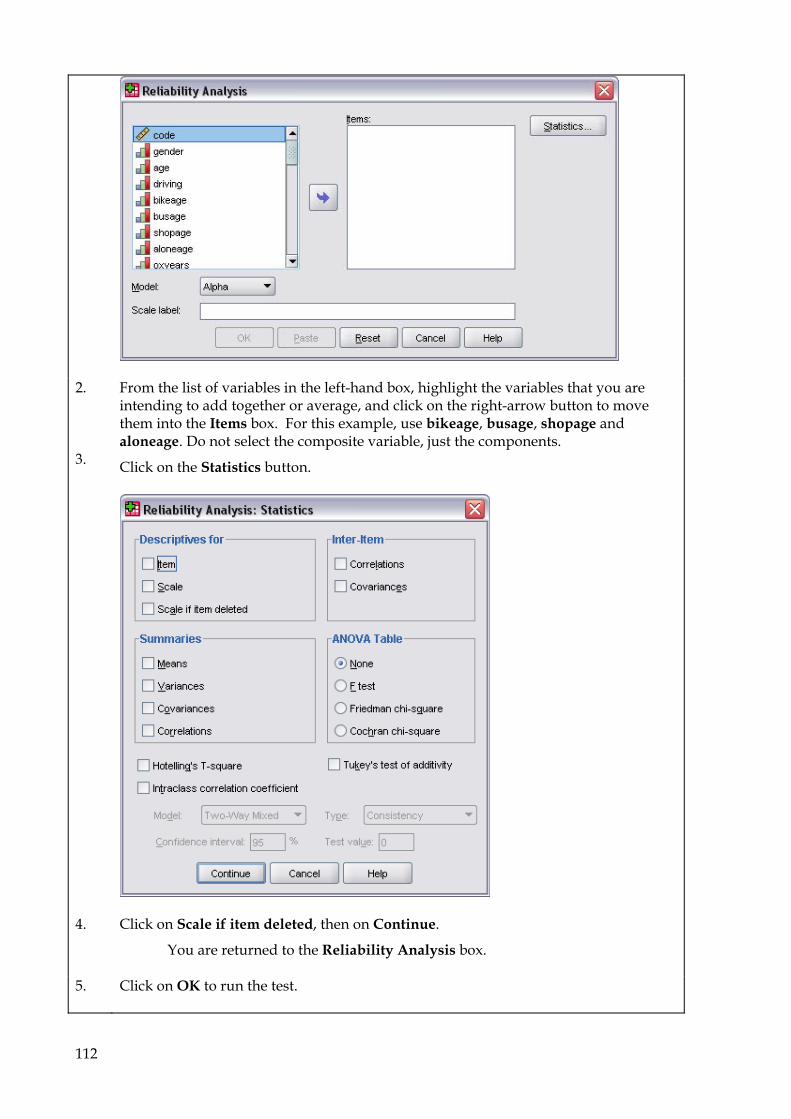
112

2. From the list of variables in the left-hand box, highlight the variables that you are intending to add together or average, and click on the right-arrow button to move them into the Items box. For this example, use bikeage, busage, shopage and aloneage. Do not select the composite variable, just the components.

3. Click on the Statistics button.

4. Click on Scale if item deleted, then on Continue.

You are returned to the Reliability Analysis box.

5. Click on OK to run the test.

113

Interpretation of results using sample questionnaire The questionnaire contains four questions asking about the ages at which the participants were allowed to do certain things. If these four variables were averaged, then the result might give an indication of how much freedom the participant had as a child. Reliability [DataSet1] U:\data\SOCSCI\spssvalues.sav

Scale: ALL VARIABLES

Case Processing Summary

N %

Cases Valid 50 92.6

Excludeda 4 7.4

Total 54 100.0

a. Listwise deletion based on all variables in the

procedure.

Reliability Statistics

Cronbach's Alpha N of Items

.639 4

Item-Total Statistics

Scale Mean if

Item Deleted

Scale Variance if

Item Deleted

Corrected Item-

Total Correlation

Cronbach's Alpha

if Item Deleted

bikeage 36.20 38.776 .072 .766

busage 30.50 28.337 .675 .437

shopage 31.08 26.157 .622 .432

aloneage 27.32 20.957 .468 .562 The overall Alpha for a scale created from these four variables is 0.639, which is not really high enough, and suggests that the four variables do not inter-correlate sufficiently to justify averaging them. However, the column labelled ‘Cronbach’s Alpha if Item Deleted’ shows that if bikeage is deleted from the scale, the Cronbach’s Alpha will increase to 0.766. Therefore, the best composite freedom variable that can be created from bikeage, busage, shopage and aloneage is an average (or total) of the three variables. Bikeage should be treated separately, or ignored.

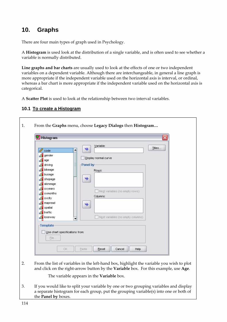
114

10. Graphs There are four main types of graph used in Psychology. A Histogram is used look at the distribution of a single variable, and is often used to see whether a variable is normally distributed. Line graphs and bar charts are usually used to look at the effects of one or two independent variables on a dependent variable. Although there are interchangeable, in general a line graph is more appropriate if the independent variable used on the horizontal axis is interval, or ordinal, whereas a bar chart is more appropriate if the independent variable used on the horizontal axis is categorical. A Scatter Plot is used to look at the relationship between two interval variables.

10.1 To create a Histogram 1. From the Graphs menu, choose Legacy Dialogs then Histogram…

2. From the list of variables in the left-hand box, highlight the variable you wish to plot and click on the right-arrow button by the Variable box. For this example, use Age.

The variable appears in the Variable box.

3. If you would like to split your variable by one or two grouping variables and display a separate histogram for each group, put the grouping variable(s) into one or both of the Panel by boxes.

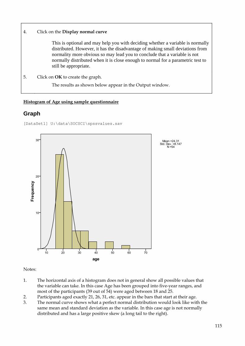
115

4. Click on the Display normal curve

This is optional and may help you with deciding whether a variable is normally distributed. However, it has the disadvantage of making small deviations from normality more obvious so may lead you to conclude that a variable is not normally distributed when it is close enough to normal for a parametric test to still be appropriate.

5. Click on OK to create the graph.

The results as shown below appear in the Output window.

Histogram of Age using sample questionnaire Graph [DataSet1] U:\data\SOCSCI\spssvalues.sav

Notes: 1. The horizontal axis of a histogram does not in general show all possible values that

the variable can take. In this case Age has been grouped into five-year ranges, and most of the participants (39 out of 54) were aged between 18 and 25.

2. Participants aged exactly 21, 26, 31, etc. appear in the bars that start at their age. 3. The normal curve shows what a perfect normal distribution would look like with the

same mean and standard deviation as the variable. In this case age is not normally distributed and has a large positive skew (a long tail to the right).

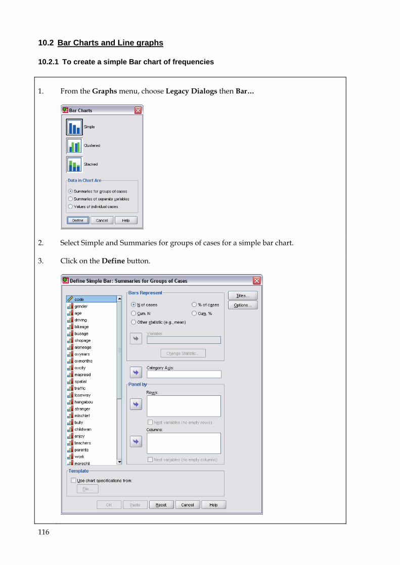
116

10.2 Bar Charts and Line graphs

10.2.1 To create a simple Bar chart of frequencies 1. From the Graphs menu, choose Legacy Dialogs then Bar…

2. Select Simple and Summaries for groups of cases for a simple bar chart.

3. Click on the Define button.

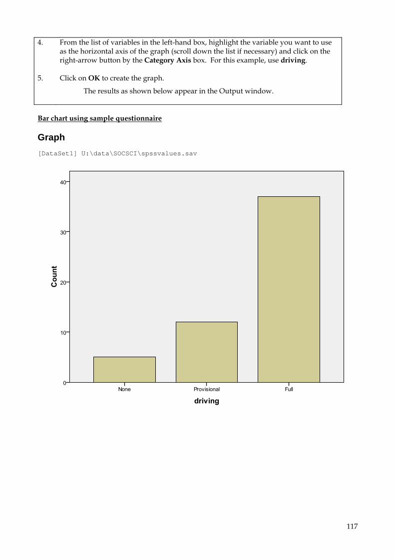
117

4. From the list of variables in the left-hand box, highlight the variable you want to use as the horizontal axis of the graph (scroll down the list if necessary) and click on the right-arrow button by the Category Axis box. For this example, use driving.

5. Click on OK to create the graph.

The results as shown below appear in the Output window.

Bar chart using sample questionnaire Graph [DataSet1] U:\data\SOCSCI\spssvalues.sav

118

10.2.2 To create a Bar chart or Line graph for independent groups Since the procedure for line graphs and bar charts is almost identical they will be dealt with together. This example will produce graphs showing the effects of Gender and attitude to public transport prices on Aloneage. This graph has been chosen for demonstration purposes and is probably not of theoretical interest. 1. From the Graphs menu, choose Legacy Dialogs then Bar…, or Line…

2. For one independent variable select Simple. For two independent variables select Clustered (for Bar Charts) or Multiple (for Line Charts). In this case there are two independent variables. For Independent groups, as in this case, select Summaries for groups of cases.

3. Click on the Define button.

The Summaries for Groups of cases box appears:

This dialogue box is identical for the two types of graph except that the top area is called either Bars Represent or Lines Represent and ‘Define Clusters by’ on the Bar Chart box is replaced with ‘Define Lines by’ on the Line chart box.

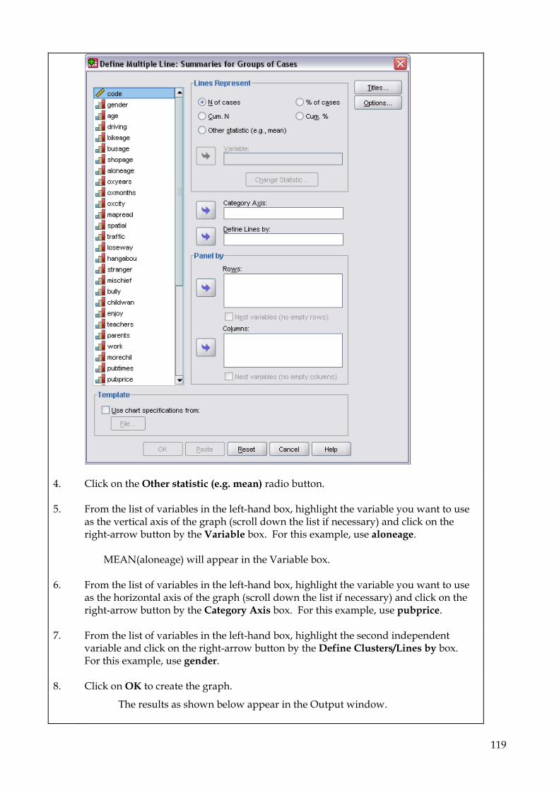
119

4. Click on the Other statistic (e.g. mean) radio button.

5. From the list of variables in the left-hand box, highlight the variable you want to use as the vertical axis of the graph (scroll down the list if necessary) and click on the right-arrow button by the Variable box. For this example, use aloneage. MEAN(aloneage) will appear in the Variable box.

6. From the list of variables in the left-hand box, highlight the variable you want to use as the horizontal axis of the graph (scroll down the list if necessary) and click on the right-arrow button by the Category Axis box. For this example, use pubprice.

7. From the list of variables in the left-hand box, highlight the second independent variable and click on the right-arrow button by the Define Clusters/Lines by box. For this example, use gender.

8. Click on OK to create the graph.

The results as shown below appear in the Output window.

120

Bar and Line charts using sample questionnaire Graph [DataSet1] U:\data\SOCSCI\spssvalues.sav

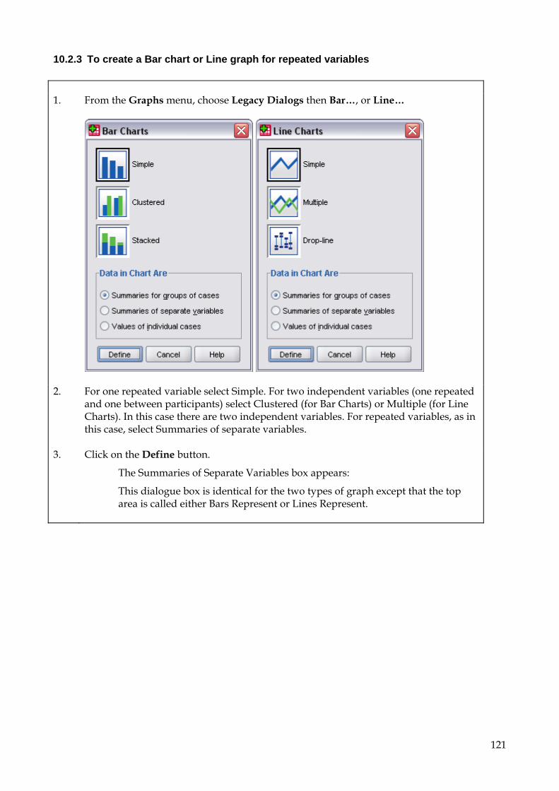
121

10.2.3 To create a Bar chart or Line graph for repeated variables 1. From the Graphs menu, choose Legacy Dialogs then Bar…, or Line…

2. For one repeated variable select Simple. For two independent variables (one repeated and one between participants) select Clustered (for Bar Charts) or Multiple (for Line Charts). In this case there are two independent variables. For repeated variables, as in this case, select Summaries of separate variables.

3. Click on the Define button.

The Summaries of Separate Variables box appears:

This dialogue box is identical for the two types of graph except that the top area is called either Bars Represent or Lines Represent.

122

4. From the list of variables in the left-hand box, highlight the variables you want to use on the vertical axis of the graph (scroll down the list if necessary) and click on the right-arrow button by the Bars/Lines Represent box. For this example, use bikeage, busage, shopage and aloneage.

The four variables will appear in the Bars/Lines Represent box in the format MEAN(bikeage), etc.

5. From the list of variables in the left-hand box, highlight the variable you want to use

as the horizontal axis of the graph (scroll down the list if necessary) and click on the right-arrow button by the Category Axis box. For this example, use gender.

6. Click on OK to create the graph.

The results as shown below appear in the Output window.

123

Bar and line charts using sample questionnaire Graph [DataSet1] U:\data\SOCSCI\spssvalues.sav

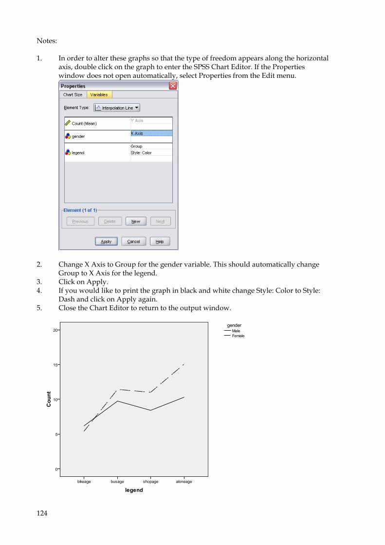
124

Notes: 1. In order to alter these graphs so that the type of freedom appears along the horizontal

axis, double click on the graph to enter the SPSS Chart Editor. If the Properties window does not open automatically, select Properties from the Edit menu.

2. Change X Axis to Group for the gender variable. This should automatically change Group to X Axis for the legend.

3. Click on Apply. 4. If you would like to print the graph in black and white change Style: Color to Style:

Dash and click on Apply again. 5. Close the Chart Editor to return to the output window.

125

10.3 To create a scatter graph 1. From the Graphs menu, choose Legacy Dialogs then Scatter/Dot…

2. Click on the Define button.

3. From the list of variables in the left-hand box, highlight the variables you want to use on the vertical axis of the graph (scroll down the list if necessary) and click on the right-arrow button by the Y Axis box. For this example, use aloneage.

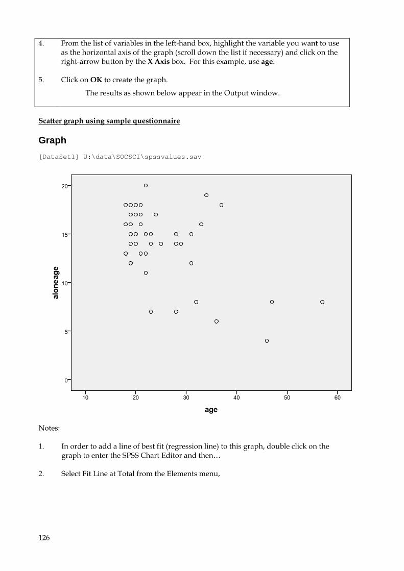
126

4. From the list of variables in the left-hand box, highlight the variable you want to use as the horizontal axis of the graph (scroll down the list if necessary) and click on the right-arrow button by the X Axis box. For this example, use age.

5. Click on OK to create the graph.

The results as shown below appear in the Output window.

Scatter graph using sample questionnaire Graph [DataSet1] U:\data\SOCSCI\spssvalues.sav

Notes: 1. In order to add a line of best fit (regression line) to this graph, double click on the

graph to enter the SPSS Chart Editor and then…

2. Select Fit Line at Total from the Elements menu,

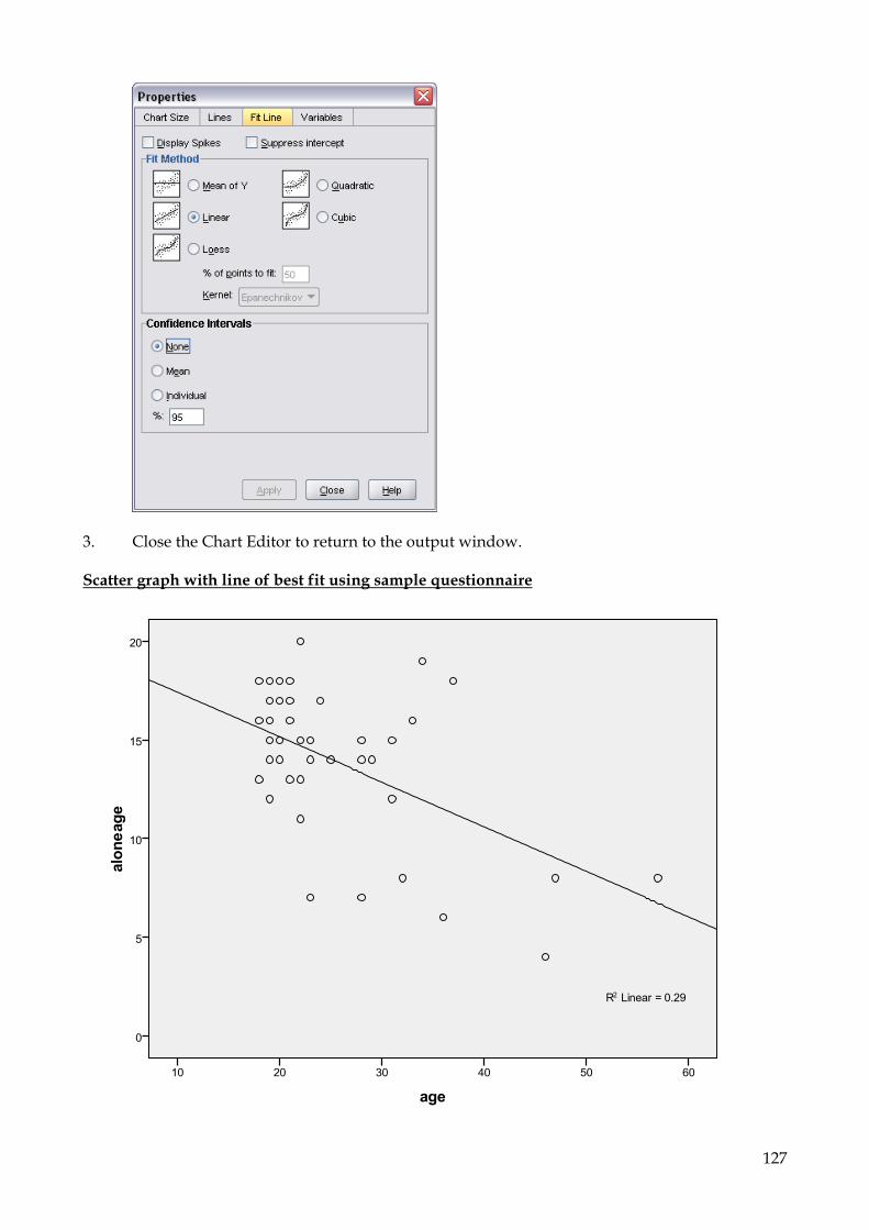
127

3. Close the Chart Editor to return to the output window. Scatter graph with line of best fit using sample questionnaire

128

11. Using your results in an assignment This section covers transferring your results into a Windows word processor. If you simply want to print directly from SPSS, follow the instructions in section 6.5.2, ‘To print all or part of your results’. Note: Students often insert the listings of all their practical results into the appendix. This is not really necessary. Before doing this think about what it might be useful to include. In your practical write-up you are trying to approximate a journal article. How often do you see a large appendix full of frequencies, and crosstabs in these? There is a happy medium, but if in doubt about how to much to include, see the tutor concerned. Unlike a journal article, however, your coursework (apart from final year dissertations) should include a ‘supporting materials’ section containing the printout for each statistical test you actually refer to in your results section.

11.1 Transferring your analysis results into Word for Windows The following ‘copy and paste’ method takes advantage of the fact that Windows can run more than one program at once. The technique may be used between most Windows programs. You simply run two programs at once - in this example, SPSS and Word - switch into the one you want to copy from, copy the text or figures you want, switch into the program you want to copy to, and paste the text or figures. Step-by-step instructions follow.

1. Run SPSS (if you haven’t already). If you have done some work and not yet saved it, now would be a good time to save.

2. Minimise SPSS by selecting the ‘Minimize’ button (looks like an underline character) in the top right hand corner of the SPSS window.

3. Locate the Word program icon and double-click it.

This runs Word for Windows, at the same time as SPSS.

4. Hold down the Alt key (to the left of the space bar on the keyboard), and press and release the Tab key (to the left of the Q). Keep pressing the Tab key until Output1 - SPSS for Windows Viewer is selected (or whichever Output window you wish to copy from) and then release the Alt key.

Your SPSS output will now come into the foreground for you to work on. A useful analogy is a desktop with several papers on it, where you simply put the piece of paper you want to work with, on the top of the pile. The SPSS Output Viewer is now at the top of the Windows pile.

5. Add any notes or make any changes you wish to the output at this stage. It is far easier to do this in SPSS than in Word. You can edit a section by double clicking on it.

6. Select the portion of the output you wish to copy by clicking on the title of the analysis (next to the yellow icon) in the left hand window. If you wish to select several portions of output at the same time then hold down the Control key while you are selecting.

129

7. Click on the Edit menu to ‘pull it down’, then click on Copy.

It may not look as though much happened - in fact, the mouse pointer changes to an hourglass for a moment - but the selected output has been copied to an area of the computer’s memory known as the Clipboard, ready to be ‘pasted’ into the Word document.

8. Switch back into Word, using Alt and Tab again.

9. Open or create the Word document into which you want to copy the material. Click at the point where you want to insert it. N.B. If you are pasting into a new document, press the Enter key a couple of times rather than pasting right at the top of the document.

10. Click on the Edit menu, then on Paste.

The SPSS output should appear where you clicked. If it doesn't, then try to Paste again. If nothing happens again, do the whole Copy and Paste again.

There is also a keyboard shortcut for Paste, normally Ctrl+V. There may also be a small picture of a glue-pot (or similar) somewhere on a toolbar at the top of the screen, which will do the same job.

11. The SPSS output is pasted into Word as tables. If a table is too large for the page, select Table, AutoFit, and then AutoFit to Window.

You may find that charts have to be copied to Word separately from the rest of your output.

12. If at any point you do something you wish you hadn’t, click on Edit then on Undo.

11.2 Final Notes Using unedited SPSS output in your results section will lose you marks! SPSS variable names should be translated into more user-friendly terms. The number of decimal places should be reduced. For variable means, I usually recommend giving one more significant figure than you are able to measure in your experiment. So if you are using a stop watch give results to the nearest tenth of a second. If you are using Superlab, milliseconds are fine. Give the standard deviations to the same number of decimal places (not significant figures) as the means. Numbers which can never be greater than 1 (e.g. p-values and correlations) can be written without a 0 before the decimal point. Numbers which can be greater than 1 (e.g. F values) should always have something before the decimal point. To reduce your word count, you can remove the spaces when reporting statistics. For example F[1, 50] = 1.72; p = .196 (seven words) can be written as F[1,50]=1.72; p=.196 (two words).

130

8.3 format for file names 17 Active cell 19 Anova 43 Anova, one-way 66 Anova, two-way 70, 76, 86, 98, 107 Avoiding repetitive work when defining

variables 20 Backing up your data 42 Cases, deleting 20 Coding variables 5 Column format 15 Command Language example 40 Compute 38 Correlation 43 Criteria, reapplying 31 Criteria, using to select cases 29 Crosstabs 43, 48 Data analysis, four steps of 10 Data file, setting up 12 Data input 19 Data, backing up 42 Data, modifying 32 Data, saving 16 Defining variables 12 Deleting a variable 20 Deleting a variable (column) or case (row

20 desktop, changing 9 Editing a Variable 16 file names, guidelines 17 Files, opening 22 Frequency analysis 23 Frequency results from Driving

questionnaire 25 Getting around 9, 27, 29, 31, 32 graph 86, 89, 91 Grouping values 32 Help, context-sensitive 11 Help, on-line 11 Highlighting/selecting text 10 If condition is satisfied’ 29 Independent t-test 53, 57, 110 Interpretation of results from Driving

questionnaire 25 Keyboard shortcuts 9 Labels for variables 15 maximising windows 9 Mean, calculating 24 Menus 9 Missing Values 14 Modifying data 32 Moving around the spreadsheet 20 Naming variables 5

Num Lock 20 Number Pad 20 Numeric keypad 20 Observed and Expected frequencies vs

Percentages 52 observed frequency 52 One-way Anova 66 On-line Help 11 On-line tutorial 11 Opening a data file 22 Output 22 Paired t-test 53 Printing the results of an analysis 27 Protecting data from accidents 42 Range, calculating 24 Recode 32 Repetitive work, avoiding 20 Results, printing 27 Results, transferring into Word for

Windows 125 Reversing values 32 Saving your data 16 significance level 52 Spreadsheet, moving around 20 Standard deviation, calculating 24 Sub-groups, selecting for analysis 29 Switching between windows 9 Transferring results into Word for

Windows 125 t-test 43, 53, 57, 110 t-test, independent 53, 57, 110 t-test, paired 53 t-test, paired, running 55, 60, 62, 64, 117 Tutorial, on-line 11 Two-way Anova 70, 76, 86, 98, 107 Type of variable 13 Value Labels 16 Variable column format 15 Variable labels 15 Variable type 13 Variables, defining 12 Variables, deleting 20 Variables, missing values in 14

131

APPENDIX 1 - EXAMPLE DATA FILE

code

gender

age

driving

bikeage

busage

shopage

aloneage

oxyears

oxmonths

oxcity

mapread

spatial

traffic

loseway

hangabou

stranger

mischief

bully

childwan

enjoy

teachers

parents

work

morechil

pubtimes

pubprice

cyclesaf

toofar

school

donethin

1 2 32 2 4 7 7 8 0 1 2 3 2 5 2 2 . 2 4 3 3 4 4 4 5 5 2 . 4 3 2

2 2 19 2 4 1 1 12 0 8 4 2 2 5 5 4 5 3 5 3 3 3 2 4 4 4 3 5 4 2 2

3 1 36 2 6 6 6 6 5 0 4 5 5 5 3 2 4 2 3 2 2 3 2 3 1 2 3 3 3 4 2

4 2 47 2 3 8 10 8 0 8 3 4 4 5 3 1 2 2 2 3 3 1 1 3 3 4 4 5 4 3 3

5 2 29 2 6 11 11 14 0 1 3 3 2 5 5 3 5 3 3 5 4 4 2 3 3 4 2 5 4 3 2

6 2 19 2 4 11 9 15 19 4 5 3 3 5 3 3 5 3 5 5 3 5 3 4 4 2 2 5 3 4 4

7 2 20 2 5 13 12 14 1 2 3 2 3 5 4 3 5 4 4 5 4 2 4 5 4 3 2 4 5 4 3

8 1 20 1 5 10 8 14 1 8 5 5 5 5 4 3 5 4 5 4 2 4 3 3 3 3 1 5 3 4 5

9 1 22 2 5 11 11 11 0 5 4 4 4 5 2 2 3 1 1 2 2 1 1 3 4 4 4 4 2 2 2

10 2 19 2 6 16 15 16 0 9 4 5 4 5 5 4 5 5 5 3 2 1 1 1 5 1 3 5 4 1 1

11 2 19 2 8 12 13 17 0 9 4 4 4 5 4 3 5 4 5 4 4 4 3 3 3 3 3 5 4 5 3

12 2 19 2 5 14 14 17 0 9 3 3 3 5 5 5 5 5 5 5 4 4 4 4 4 4 4 5 5 5 5

13 2 18 0 5 13 7 16 0 7 3 2 2 5 4 3 3 3 4 3 2 4 3 4 5 5 3 4 4 3 2

14 2 33 1 11 12 14 16 7 10 1 1 1 5 3 4 5 3 5 5 5 4 2 1 3 3 2 5 4 4 4

15 2 22 0 6 9 11 15 3 7 4 2 2 5 3 3 5 4 5 3 4 4 4 5 4 3 3 4 3 4 2

16 2 24 2 4 11 11 17 3 1 3 3 3 5 2 2 1 1 2 5 5 3 2 4 4 1 2 3 3 3 3

17 2 57 2 10 10 8 8 3 0 3 4 3 5 3 4 5 3 5 4 4 4 3 3 3 4 2 4 3 3 2

18 2 28 2 . 12 14 14 0 8 2 3 2 3 3 1 2 1 1 1 4 4 3 5 5 4 2 . 2 2 1

19 2 19 2 4 13 13 17 0 8 3 2 2 5 5 4 5 4 5 4 2 4 3 2 2 4 4 5 4 4 2

20 2 20 2 4 12 12 18 5 0 4 4 2 4 2 5 5 4 4 5 5 4 4 5 4 5 2 5 3 5 5

21 1 20 1 12 12 12 14 0 8 4 4 4 5 5 3 4 4 5 5 5 3 3 4 4 4 2 4 5 5 2

22 2 19 2 4 12 10 14 0 8 3 4 2 5 3 3 4 3 3 2 3 4 4 4 3 2 2 3 2 3 3

23 2 20 2 6 10 10 15 20 8 4 5 4 4 2 2 3 2 . 3 3 1 4 1 3 . 1 4 3 3 2

24 2 22 2 3 14 14 20 0 7 4 4 3 4 5 2 5 2 3 5 5 5 5 5 4 4 1 5 1 4 3

25 2 19 2 4 11 9 14 0 8 2 3 2 4 5 3 4 4 5 5 3 2 1 4 4 4 4 4 4 4 3

26 2 19 0 4 12 12 14 1 8 4 2 2 4 5 3 5 3 4 5 5 5 5 5 5 5 2 5 5 5 4

27 2 19 1 5 12 12 16 0 9 3 4 2 4 4 2 5 2 3 4 3 3 3 4 1 4 2 5 4 2 2

132

code

gender

age

driving

bikeage

busage

shopage

aloneage

oxyears

oxmonths

oxcity

mapread

spatial

traffic

loseway

hangabou

stranger

mischief

bully

childwan

enjoy

teachers

parents

work

morechil

pubtimes

pubprice

cyclesaf

toofar

school

donethin

28 2 25 1 8 12 12 14 3 5 4 4 4 5 3 3 4 3 4 4 5 2 2 1 1 1 2 2 3 3 3

29 2 46 1 . 15 18 4 2 0 3 3 4 4 4 3 3 3 4 4 3 2 2 . 1 1 1 5 5 3 .

30 2 37 2 12 13 9 18 12 0 3 2 2 3 3 3 2 2 3 3 4 3 3 3 3 3 3 3 3 4 4

31 2 19 1 5 12 12 12 0 9 3 4 2 5 4 2 5 2 3 2 2 3 3 4 1 4 2 5 4 3 1

32 2 21 2 2 11 11 13 1 0 4 4 4 5 5 4 5 4 5 5 4 4 3 4 4 4 4 5 3 4 4

33 2 21 1 . 10 12 16 2 0 4 4 3 5 5 5 5 5 5 5 5 4 4 4 4 5 3 5 4 4 5

34 2 20 2 5 10 10 14 0 9 4 4 3 5 4 4 5 5 5 4 3 3 4 4 4 4 3 5 4 4 3

35 2 19 2 5 11 11 16 0 9 4 3 2 4 4 4 5 3 4 2 3 4 2 4 5 4 4 4 2 2 2

36 2 18 1 5 13 13 13 0 10 4 2 3 5 4 4 4 3 3 3 2 1 2 4 4 4 2 4 3 3 2

37 2 23 2 7 11 14 14 0 0 2 4 2 5 5 3 5 3 3 2 1 2 1 3 1 4 4 5 4 3 1

38 2 19 2 8 10 11 14 0 10 2 2 3 5 4 3 4 3 4 3 3 2 2 3 3 4 2 3 3 3 1

39 2 19 1 5 11 11 18 0 9 3 4 2 5 3 3 4 3 5 3 3 4 3 3 4 4 4 4 3 3 2

40 2 21 2 4 11 12 18 0 8 2 4 4 5 3 4 5 4 4 5 4 2 2 4 4 5 4 5 1 3 2

41 2 28 2 7 14 12 14 3 10 5 3 2 5 3 2 2 2 2 3 3 3 3 4 4 3 2 4 2 2 2

42 2 31 2 6 14 12 15 0 0 2 2 3 5 2 2 5 5 5 2 2 2 1 3 4 4 4 3 4 3 2

43 2 18 1 5 11 11 18 0 9 2 3 3 5 4 4 4 2 5 5 5 5 4 2 2 4 3 5 3 5 2

44 2 23 0 3 10 9 15 3 10 5 4 4 5 5 3 4 2 5 5 5 3 2 5 5 5 1 5 2 1 1

45 2 19 2 4 9 9 17 0 9 3 5 3 5 4 3 4 4 5 5 1 1 1 2 2 4 1 4 3 3 2

46 2 28 2 5 11 11 15 3 8 4 4 4 5 5 2 5 3 4 5 4 4 4 4 4 3 3 5 3 3 1

47 1 22 2 6 10 8 13 1 2 3 4 4 5 3 2 3 2 3 2 3 4 3 4 3 4 3 3 2 3 3

48 2 21 2 3 13 10 17 4 5 5 5 4 5 3 2 5 3 5 5 2 1 1 2 . 4 2 2 1 1 1

49 2 31 2 5 12 11 12 28 7 4 5 5 5 5 4 5 3 4 5 2 1 1 3 3 4 4 5 2 4 2

50 1 23 1 5 10 7 7 0 2 2 3 3 3 3 2 3 3 3 4 5 2 2 3 4 4 3 5 2 3 4

51 1 28 2 4 9 7 7 3 0 4 4 4 3 1 2 4 3 3 4 1 1 1 1 3 2 4 2 3 3 3

52 2 19 0 6 8 5 15 1 9 5 2 1 5 3 4 5 4 4 2 1 2 2 1 2 3 1 5 3 3 2

53 2 20 2 6 11 11 17 0 9 4 4 3 5 3 3 4 3 5 4 3 2 3 4 2 4 4 4 2 4 3

54 2 34 2 5 11 11 19 0 201 1 3 4 5 5 3 5 4 4 2 3 3 3 4 3 2 2 5 2 3 2

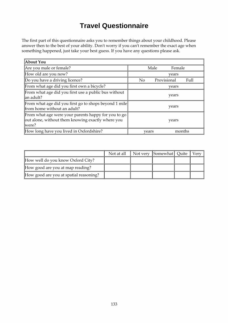
133

Travel Questionnaire

The first part of this questionnaire asks you to remember things about your childhood. Please answer then to the best of your ability. Don't worry if you can't remember the exact age when something happened, just take your best guess. If you have any questions please ask.

About You Are you male or female? Male Female How old are you now? years Do you have a driving licence? No Provisional Full From what age did you first own a bicycle? years From what age did you first use a public bus without an adult? years

From what age did you first go to shops beyond 1 milefrom home without an adult? years

From what age were your parents happy for you to go out alone, without them knowing exactly where you were?

years

How long have you lived in Oxfordshire? years months

Not at all Not very Somewhat Quite Very How well do you know Oxford City? How good are you at map reading? How good are you at spatial reasoning?

134

Imagine that you live at the edge of a small town (such as Bicester or Witney) and have a 9 year old child, the same gender as yourself, who has to travel 1-2 miles (1.6-3.2 kilometres) to get to school. Walking would take 20-40 minutes each way) and involve crossing one or two main roads (at crossings) plus a few minor roads. How important do you think each of the following factors would be, when deciding whether or not you would accompany your child on the journey to school? When deciding whether to accompany my child to school I would consider whether...

Not at all important

Not very important

Somewhatimportant

Quite important

Very important

my child might not be careful of traffic my child might lose way my child might hang about on way my child might talk to strangers my child might be mischievous my child might bully or be bullied my child might want me to be with them I might enjoy taking my child I might want to talk to teachers I might want to talk to other parents I might travel to work that way anyway I might have another child at the same school

the public transport times might be inconvenient

the public transport might be expensive my child might not be able to cycle safely 1 mile is okay but a 2 mile journey would be too far

the School might prefer children to be accompanied

accompanying is the done thing