SQL Server Architecture - Wiley · As shown in Figure 1-1, SQL Server is split into two main engines: the Relational Engine and the Storage Engine. The Relational Engine is also sometimes

SQL Server Architecture

WHAT’S IN THIS CHAPTER

Understanding database transactions and the ACID properties ➤

Architectural components used to fulfi ll a read request ➤

Architectural components used to fulfi ll an update request ➤

Database recovery and the transaction log ➤

Dirty pages, checkpoints, and the lazywriter ➤

Where the SQLOS fi ts in and why it’s needed ➤

A basic grasp of SQL Server’s architecture is fundamental to intelligently approach trouble-shooting a problem, but selecting the important bits to learn about can be challenging, as SQL Server is such a complex piece of software.

This chapter distills the core architecture of SQL Server and puts the most important compo-nents into the context of executing a simple query to help you understand the fundamentals of the core engine.

You will learn how SQL Server deals with your network connection, unravels what you’re asking it to do, decides how it will execute your request, and fi nally how data is retrieved and modifi ed on your behalf.

You will also discover when the transaction log is used and how it’s affected by the confi gured recovery model; what happens when a checkpoint occurs and how you can infl uence the fre-quency; and what the lazywriter does.

1

84289c01.indd 184289c01.indd 1 11/23/09 4:11:23 PM11/23/09 4:11:23 PM

COPYRIG

HTED M

ATERIAL

2 ❘ CHAPTER 1 SQL SERVER ARCHITECTURE

The chapter starts by defi ning a “transaction” and what the requirements are for a database system to reliably process them. You’ll then look at the life cycle of a simple query that reads data, taking a walk through the components employed to return a result set, before looking at how the process dif-fers when data needs to be modifi ed.

Finally, you’ll read about the components and terminology that support the recovery process in SQL Server, and the SQLOS “framework” introduced in SQL Server 2005 that consolidates a lot of the low-level functions required by many SQL Server components.

Some areas of the life cycle described in this chapter are intentionally shallow in order to keep the fl ow manageable, and where that’s the case you are directed to the chapter or chapters that cover the topic in more depth.

DATABASE TRANSACTIONS

A transaction is a unit of work in a database that typically contains several commands that read from and write to the database. The most well-known feature of a transaction is that it must com-plete all of the commands in their entirety or none of them. This feature, called atomicity, is just one of four properties defi ned in the early days of database theory as requirements for a database trans-action, collectively known as ACID properties.

ACID Properties

The four required properties of a database transaction are atomicity, consistency, isolation, and durability.

Atomicity

Atomicity means that all the effects of the transaction must complete successfully or the changes are rolled back. A classic example of an atomic transaction is a withdrawal from an ATM machine; the machine must both dispense the cash and debit your bank account. Either of those actions complet-ing independently would cause a problem for either you or the bank.

Consistency

The consistency requirement ensures that the transaction cannot break the integrity rules of the database; it must leave the database in a consistent state. For example, your system might require that stock levels cannot be a negative value, a spare part cannot exist without a parent object, or the data in a sex fi eld must be male or female. In order to be consistent, a transaction must not break any of the constraints or rules defi ned for the data.

84289c01.indd 284289c01.indd 2 11/23/09 4:11:23 PM11/23/09 4:11:23 PM

The Life Cycle of a Query ❘ 3

Isolation

Isolation refers to keeping the changes of incomplete transactions running at the same time separate from one another. Each transaction must be entirely self-contained, and changes it makes must not be readable by any other transaction, although SQL Server does allow you to control the degree of isolation in order to fi nd a balance between business and performance requirements.

Durability

Once a transaction is committed, it must persist even if there is a system failure — that is, it must be durable. In SQL Server, the information needed to replay changes made in a transaction is written to the transaction log before the transaction is considered to be committed.

SQL Server Transactions

There are two types of transactions in SQL Server that are differentiated only by the way they are created: implicit and explicit.

Implicit transactions are used automatically by SQL Server to guarantee the ACID properties of single commands. For example, if you wrote an update statement that modifi ed 10 rows, SQL Server would run it as an implicit transaction so that the ACID properties would apply, and all 10 rows would be updated or none of them would.

Explicit transactions are started by using the BEGIN TRANSACTION T-SQL command and are stopped by using the COMMIT TRANSACTION or ROLLBACK TRANSACTION commands.

Committing a transaction effectively means making the changes within the transaction permanent, whereas rolling back a transaction means undoing all the changes that were made within the trans-action. Explicit transactions are used to group together changes to which you want to apply the ACID properties as a whole, which also enables you to roll back the changes at any point if your business logic determines that you should cancel the change.

THE LIFE CYCLE OF A QUERY

To introduce the high-level components of SQL Server’s architecture, this section uses the example of a query’s life cycle to put each component into context in order to foster your understanding and create a foundation for the rest of the book.

It looks at a basic SELECT query fi rst in order to reduce the scope to that of a READ operation, and then introduces the additional processes involved for a query that performs an UPDATE operation. Finally, you’ll read about the terminology and processes that SQL Server uses to implement recovery while optimizing performance.

Figure 1-1 shows the high-level components that are used within the chapter to illustrate the life cycle of a query.

84289c01.indd 384289c01.indd 3 11/23/09 4:11:23 PM11/23/09 4:11:23 PM


Cmd Parser

Query Executor

Access Methods

TransactionMgr

BufferManager

Optimizer SNISQL Server

Network Interface

ProtocolLayerRelational Engine

Storage Engine Buffer Pool

Plan Cache

Data CacheData file

Transaction Log

FIGURE 1-1

The Relational and Storage Engines

As shown in Figure 1-1, SQL Server is split into two main engines: the Relational Engine and the Storage Engine.

The Relational Engine is also sometimes called the query processor because its primary function is query optimization and execution. It contains a Command Parser to check query syntax and pre-pare query trees, a Query Optimizer that is arguably the crown jewel of any database system, and a Query Executor responsible for execution.

The Storage Engine is responsible for managing all I/O to the data, and contains the Access Methods code, which handles I/O requests for rows, indexes, pages, allocations and row versions, and a Buffer Manager, which deals with SQL Server’s main memory consumer, the buffer pool. It also contains a Transaction Manager, which handles the locking of data to maintain Isolation (ACID properties) and manages the transaction log.

The Buff er Pool

The other major component you need to know about before getting into the query life cycle is the buffer pool, which is the largest consumer of memory in SQL Server. The buffer pool contains all

84289c01.indd 484289c01.indd 4 11/23/09 4:11:23 PM11/23/09 4:11:23 PM


the different caches in SQL Server, including the plan cache and the data cache, which is covered as the sections follow the query through its life cycle.

The buffer pool is covered in detail in Chapter 2.

A Basic Select Query

The details of the query used in this example aren’t important — it’s a simple SELECT statement with no joins, so you’re just issuing a basic read request. Start at the client, where the fi rst component you touch is the SQL Server Network Interface (SNI).

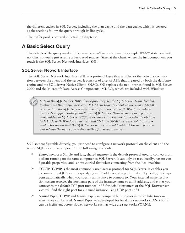
SQL Server Network Interface

The SQL Server Network Interface (SNI) is a protocol layer that establishes the network connec-tion between the client and the server. It consists of a set of APIs that are used by both the database engine and the SQL Server Native Client (SNAC). SNI replaces the net-libraries found in SQL Server 2000 and the Microsoft Data Access Components (MDAC), which are included with Windows.

Late in the SQL Server 2005 development cycle, the SQL Server team decided to eliminate their dependence on MDAC to provide client connectivity. MDAC is owned by the SQL Server team but ships in the box with Windows, which means its shipped ‘out-of-band’ with SQL Server. With so many new features being added in SQL Server 2005, it became cumbersome to coordinate updates to MDAC with Windows releases, and SNI and SNAC were the solutions cre-ated. This meant that the SQL Server team could add support for new features and release the new code in-line with SQL Server releases.

SNI isn’t confi gurable directly; you just need to confi gure a network protocol on the client and the server. SQL Server has support for the following protocols:

Shared memory: ➤ Simple and fast, shared memory is the default protocol used to connect from a client running on the same computer as SQL Server. It can only be used locally, has no con-fi gurable properties, and is always tried fi rst when connecting from the local machine.

TCP/IP: ➤ TCP/IP is the most commonly used access protocol for SQL Server. It enables you to connect to SQL Server by specifying an IP address and a port number. Typically, this hap-pens automatically when you specify an instance to connect to. Your internal name resolu-tion system resolves the hostname part of the instance name to an IP address, and either you connect to the default TCP port number 1433 for default instances or the SQL Browser ser-vice will fi nd the right port for a named instance using UDP port 1434.

Named Pipes: ➤ TCP/IP and Named Pipes are comparable protocols in the architectures in which they can be used. Named Pipes was developed for local area networks (LANs) but it can be ineffi cient across slower networks such as wide area networks (WANs).

84289c01.indd 584289c01.indd 5 11/23/09 4:11:23 PM11/23/09 4:11:23 PM


To use Named Pipes you fi rst need to enable it in SQL Server Confi guration Manager (if you’ll be connecting remotely) and then create a SQL Server alias, which connects to the server using Named Pipes as the protocol.

Named Pipes uses TCP port 445, so ensure that the port is open on any fi rewalls between the two computers, including the Windows Firewall.

VIA: ➤ Virtual Interface Adapter is a protocol that enables high-performance communica-tions between two systems. It requires specialized hardware at both ends and a dedicated connection.

Like Named Pipes, to use the VIA protocol you fi rst need to enable it in SQL Server Con-fi guration Manager and then create a SQL Server alias that connects to the server using VIA as the protocol.

Regardless of the network protocol used, once the connection is established, SNI creates a secure connection to a TDS endpoint (described next) on the server, which is then used to send requests and receive data. For the purpose here of following a query through its life cycle, you’re sending the SELECT statement and waiting to receive the result set.

TDS (Tabular Data Stream) Endpoints

TDS is a Microsoft-proprietary protocol originally designed by Sybase that is used to interact with a database server. Once a connection has been made using a network protocol such as TCP/IP, a link is established to the relevant TDS endpoint that then acts as the communication point between the client and the server.

There is one TDS endpoint for each network protocol and an additional one reserved for use by the dedicated administrator connection (DAC). Once connectivity is established, TDS messages are used to communicate between the client and the server.

The SELECT statement is sent to the SQL Server as a TDS message across a TCP/IP connection (TCP/IP is the default protocol).

Protocol Layer

When the protocol layer in SQL Server receives your TDS packet, it has to reverse the work of the SNI at the client and unwrap the packet to fi nd out what request it contains. The protocol layer is also responsible for packaging up results and status messages to send back to the client as TDS messages.

Our SELECT statement is marked in the TDS packet as a message of type “SQL Command,” so it’s passed on to the next component, the Query Parser, to begin the path toward execution.

Figure 1-2 shows where our query has gone so far. At the client, the statement was wrapped in a TDS packet by the SQL Server Network Interface and sent to the protocol layer on the SQL Server where it was unwrapped, identifi ed as a SQL Command, and the code sent to the Command Parser by the SNI.

84289c01.indd 684289c01.indd 6 11/23/09 4:11:24 PM11/23/09 4:11:24 PM


Cmd Parser

Query ExecutorOptimizer SNISQL Server

Network Interface


TDS

Language Event

FIGURE 1-2

Command Parser

The Command Parser’s role is to handle T-SQL language events. It fi rst checks the syntax and returns any errors back to the protocol layer to send to the client. If the syntax is valid, then the next step is to generate a query plan or fi nd an existing plan. A query plan contains the details about how SQL Server is going to execute a piece of code. It is commonly referred to as an execution plan.

To check for a query plan, the Command Parser generates a hash of the T-SQL and checks it against the plan cache to determine whether a suitable plan already exists. The plan cache is an area in the buffer pool used to cache query plans. If it fi nds a match, then the plan is read from cache and passed on to the Query Executor for execution. (The following section explains what happens if it doesn’t fi nd a match.)

Plan Cache

Creating execution plans can be time consuming and resource intensive, so it makes sense that if SQL Server has already found a good way to execute a piece of code that it should try to reuse it for subsequent requests.

The plan cache, part of SQL Server’s buffer pool, is used to store execution plans in case they are needed later. You can read more about execution plans and plan cache in Chapters 2 and 5.

If no cached plan is found, then the Command Parser generates a query tree based on the T-SQL. A query tree is an internal structure whereby each node in the tree represents an operation in the query that needs to be performed. This tree is then passed to the Query Optimizer to process.

Our basic query didn’t have an existing plan so a query tree was created and passed to the Query Optimizer.

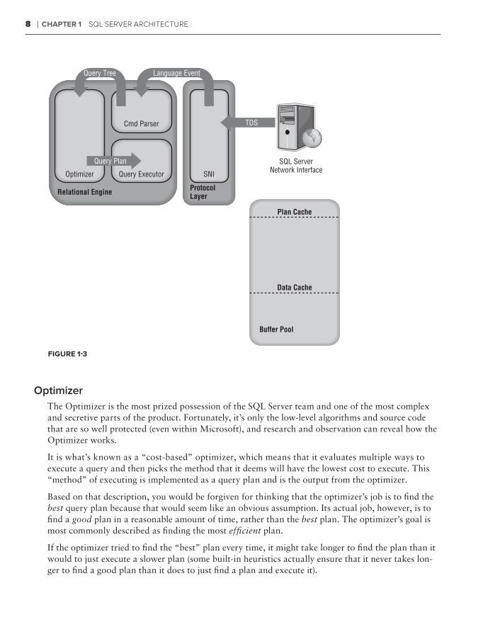
Figure 1-3 shows the plan cache added to the diagram, which is checked by the Command Parser for an existing query plan. Also added is the query tree output from the Command Parser being passed to the optimizer because nothing was found in cache for our query.

84289c01.indd 784289c01.indd 7 11/23/09 4:11:24 PM11/23/09 4:11:24 PM


Cmd Parser

Query ExecutorOptimizer SNI

SQL ServerNetwork Interface


Buffer Pool

Plan Cache

Data Cache

TDS

Query Plan

Language EventQuery Tree

FIGURE 1-3

Optimizer

The Optimizer is the most prized possession of the SQL Server team and one of the most complex and secretive parts of the product. Fortunately, it’s only the low-level algorithms and source code that are so well protected (even within Microsoft), and research and observation can reveal how the Optimizer works.

It is what’s known as a “cost-based” optimizer, which means that it evaluates multiple ways to execute a query and then picks the method that it deems will have the lowest cost to execute. This “method” of executing is implemented as a query plan and is the output from the optimizer.

Based on that description, you would be forgiven for thinking that the optimizer’s job is to fi nd the best query plan because that would seem like an obvious assumption. Its actual job, however, is to fi nd a good plan in a reasonable amount of time, rather than the best plan. The optimizer’s goal is most commonly described as fi nding the most effi cient plan.

If the optimizer tried to fi nd the “best” plan every time, it might take longer to fi nd the plan than it would to just execute a slower plan (some built-in heuristics actually ensure that it never takes lon-ger to fi nd a good plan than it does to just fi nd a plan and execute it).

84289c01.indd 884289c01.indd 8 11/23/09 4:11:24 PM11/23/09 4:11:24 PM


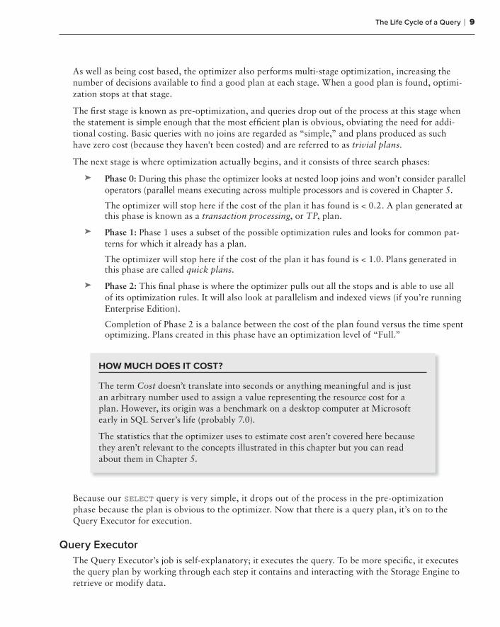
As well as being cost based, the optimizer also performs multi-stage optimization, increasing the number of decisions available to fi nd a good plan at each stage. When a good plan is found, optimi-zation stops at that stage.

The fi rst stage is known as pre-optimization, and queries drop out of the process at this stage when the statement is simple enough that the most effi cient plan is obvious, obviating the need for addi-tional costing. Basic queries with no joins are regarded as “simple,” and plans produced as such have zero cost (because they haven’t been costed) and are referred to as trivial plans.

The next stage is where optimization actually begins, and it consists of three search phases:

Phase 0: ➤ During this phase the optimizer looks at nested loop joins and won’t consider parallel operators (parallel means executing across multiple processors and is covered in Chapter 5.

The optimizer will stop here if the cost of the plan it has found is < 0.2. A plan generated at this phase is known as a transaction processing, or TP, plan.

Phase 1: ➤ Phase 1 uses a subset of the possible optimization rules and looks for common pat-terns for which it already has a plan.

The optimizer will stop here if the cost of the plan it has found is < 1.0. Plans generated in this phase are called quick plans.

Phase 2: ➤ This fi nal phase is where the optimizer pulls out all the stops and is able to use all of its optimization rules. It will also look at parallelism and indexed views (if you’re running Enterprise Edition).

Completion of Phase 2 is a balance between the cost of the plan found versus the time spent optimizing. Plans created in this phase have an optimization level of “Full.”

HOW MUCH DOES IT COST?

The term Cost doesn’t translate into seconds or anything meaningful and is just an arbitrary number used to assign a value representing the resource cost for a plan. However, its origin was a benchmark on a desktop computer at Microsoft early in SQL Server’s life (probably 7.0).

The statistics that the optimizer uses to estimate cost aren’t covered here because they aren’t relevant to the concepts illustrated in this chapter but you can read about them in Chapter 5.

Because our SELECT query is very simple, it drops out of the process in the pre-optimization phase because the plan is obvious to the optimizer. Now that there is a query plan, it’s on to the Query Executor for execution.

Query Executor

The Query Executor’s job is self-explanatory; it executes the query. To be more specifi c, it executes the query plan by working through each step it contains and interacting with the Storage Engine to retrieve or modify data.

84289c01.indd 984289c01.indd 9 11/23/09 4:11:24 PM11/23/09 4:11:24 PM


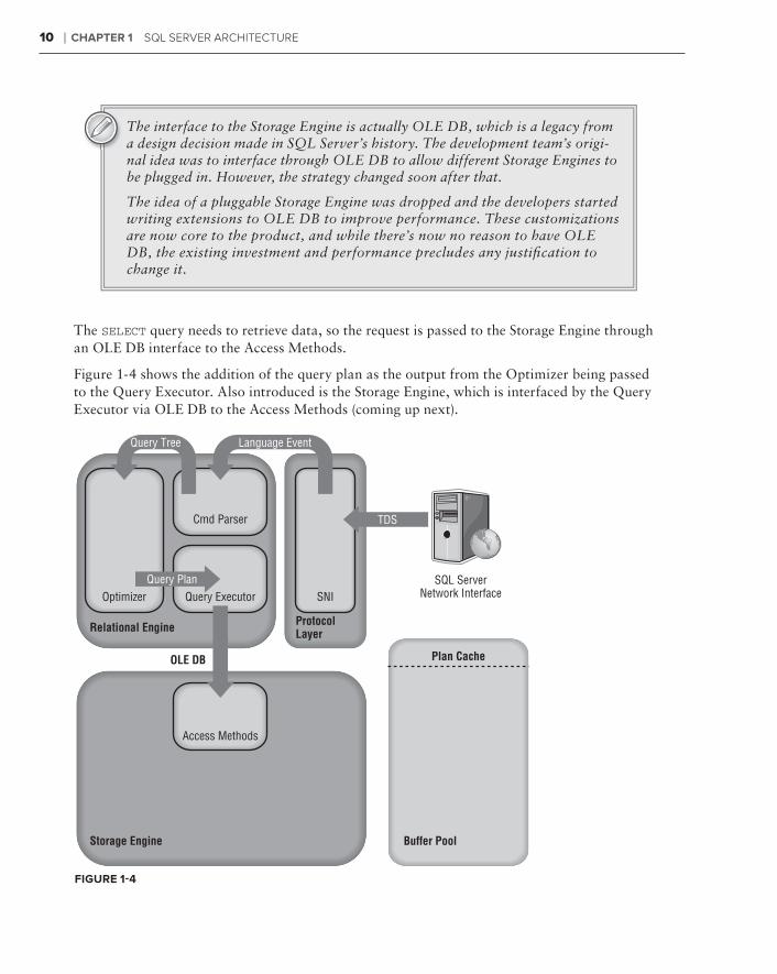
The interface to the Storage Engine is actually OLE DB, which is a legacy from a design decision made in SQL Server’s history. The development team’s origi-nal idea was to interface through OLE DB to allow different Storage Engines to be plugged in. However, the strategy changed soon after that.

The idea of a pluggable Storage Engine was dropped and the developers started writing extensions to OLE DB to improve performance. These customizations are now core to the product, and while there’s now no reason to have OLE DB, the existing investment and performance precludes any justifi cation to change it.

The SELECT query needs to retrieve data, so the request is passed to the Storage Engine through an OLE DB interface to the Access Methods.

Figure 1-4 shows the addition of the query plan as the output from the Optimizer being passed to the Query Executor. Also introduced is the Storage Engine, which is interfaced by the Query Executor via OLE DB to the Access Methods (coming up next).

Cmd Parser

Query Executor

Access Methods


Network Interface


Storage Engine

OLE DB

Buffer Pool

Plan Cache

TDS

Query Plan


FIGURE 1-4

84289c01.indd 1084289c01.indd 10 11/23/09 4:11:24 PM11/23/09 4:11:24 PM


Access Methods

Access Methods is a collection of code that provides the storage structures for your data and indexes as well as the interface through which data is retrieved and modifi ed. It contains all the code to retrieve data but it doesn’t actually perform the operation itself; it passes the request to the Buffer Manager.

Suppose our SELECT statement needs to read just a few rows that are all on a single page. The Access Methods code will ask the Buffer Manager to retrieve the page so that it can prepare an OLE DB rowset to pass back to the Relational Engine.

Buff er Manager

The Buffer Manager, as its name suggests, manages the buffer pool, which represents the majority of SQL Server’s memory usage.

If you need to read some rows from a page (you’ll look at writes when we look at an UPDATE query) the Buffer Manager will check the data cache in the buffer pool to see if it already has the page cached in memory. If the page is already cached, then the results are passed back to the Access Methods.

If the page isn’t already in cache, then the Buffer Manager will get the page from the database on disk, put it in the data cache, and pass the results to the Access Methods.

The PAGEIOLATCH wait type represents the time it takes to read a data page from disk into memory. You can read about wait types in Chapter 3.

The key point to take away from this is that you only ever work with data in memory. Every new data read that you request is fi rst read from disk and then written to memory (the data cache) before being returned to you as a result set.

This is why SQL Server needs to maintain a minimum level of free pages in memory; you wouldn’t be able to read any new data if there were no space in cache to put it fi rst.

The Access Methods code determined that the SELECT query needed a single page, so it asked the Buffer Manager to get it. The Buffer Manager checked to see whether it already had it in the data cache, and then loaded it from disk into the cache when it couldn’t fi nd it.

Data Cache

The data cache is usually the largest part of the buffer pool; therefore, it’s the largest memory con-sumer within SQL Server. It is here that every data page that is read from disk is written to before being used.

The sys.dm_os_buffer_descriptors DMV contains one row for every data page currently held in cache. You can use this script to see how much space each database is using in the data cache:

SELECT count(*)*8/1024 AS ‘Cached Size (MB)’ ,CASE database_id WHEN 32767 THEN ‘ResourceDb’

84289c01.indd 1184289c01.indd 11 11/23/09 4:11:24 PM11/23/09 4:11:24 PM


ELSE db_name(database_id) END AS ‘Database’FROM sys.dm_os_buffer_descriptorsGROUP BY db_name(database_id) ,database_idORDER BY ‘Cached Size (MB)’ DESC

The output will look something like this (with your own databases obviously):

Cached Size (MB) Database3287 People34 tempdb12 ResourceDb4 msdb

In this example, the People database has 3,287MB of data pages in the data cache.

The amount of time that pages stay in cache is determined by a least recently used (LRU) policy.

The header of each page in cache stores details about the last two times it was accessed, and a peri-odic scan through the cache examines these values. A counter is maintained that is decremented if the page hasn’t been accessed for a while; and when SQL Server needs to free up some cache, the pages with the lowest counter are fl ushed fi rst.

The process of “aging out” pages from cache and maintaining an available amount of free cache pages for subsequent use can be done by any worker thread after scheduling its own I/O or by the lazywriter process, covered later in the section “Lazywriter.”

You can view how long SQL Server expects to be able to keep a page in cache by looking at the MSSQL$<instance>:Buffer Manager\Page Life Expectancy counter in Performance Monitor. Page life expectancy (PLE) is the amount of time, in seconds, that SQL Server expects to be able to keep a page in cache.

Under memory pressure, data pages are fl ushed from cache far more frequently. Microsoft recom-mends a minimum of 300 seconds for a good PLE, but for systems with plenty of physical memory this will easily reach thousands of seconds.

The database page read to serve the result set for our SELECT query is now in the data cache in the buffer pool and will have an entry in the sys.dm_os_buffer_descriptors DMV. Now that the Buffer Manager has the result set, it’s passed back to the Access Methods to make its way to the client.

A Basic select Statement Life Cycle Summary

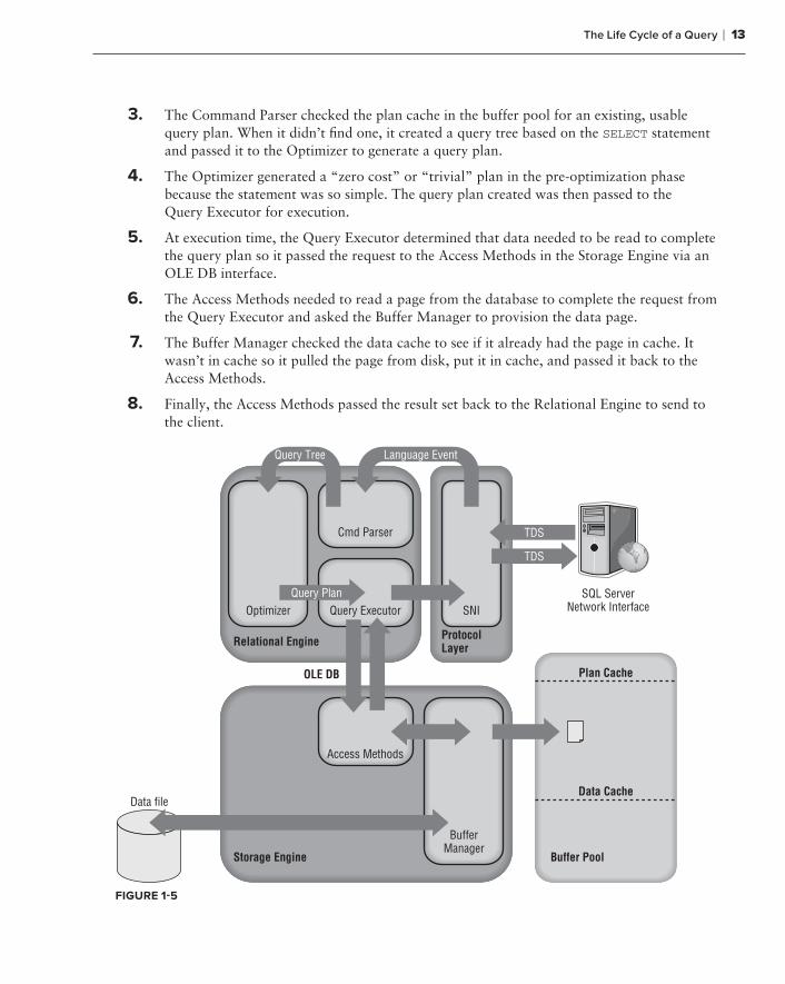
Figure 1-5 shows the whole life cycle of a SELECT query, described here:

1. The SQL Server Network Interface (SNI) on the client established a connection to the SNI on the SQL Server using a network protocol such as TCP/IP. It then created a connection to a TDS endpoint over the TCP/IP connection and sent the SELECT statement to SQL Server as a TDS message.

2. The SNI on the SQL Server unpacked the TDS message, read the SELECT statement, and passed a “SQL Command” to the Command Parser.

84289c01.indd 1284289c01.indd 12 11/23/09 4:11:24 PM11/23/09 4:11:24 PM


3. The Command Parser checked the plan cache in the buffer pool for an existing, usable query plan. When it didn’t fi nd one, it created a query tree based on the SELECT statement and passed it to the Optimizer to generate a query plan.

4. The Optimizer generated a “zero cost” or “trivial” plan in the pre-optimization phase because the statement was so simple. The query plan created was then passed to the Query Executor for execution.

5. At execution time, the Query Executor determined that data needed to be read to complete the query plan so it passed the request to the Access Methods in the Storage Engine via an OLE DB interface.

6. The Access Methods needed to read a page from the database to complete the request from the Query Executor and asked the Buffer Manager to provision the data page.

7. The Buffer Manager checked the data cache to see if it already had the page in cache. It wasn’t in cache so it pulled the page from disk, put it in cache, and passed it back to the Access Methods.

8. Finally, the Access Methods passed the result set back to the Relational Engine to send to the client.

Cmd Parser

Query Executor

Access Methods

BufferManager


Network Interface


Storage Engine

OLE DB

Buffer Pool

Plan Cache

Data CacheData file

TDS

TDS

Query Plan


FIGURE 1-5

84289c01.indd 1384289c01.indd 13 11/23/09 4:11:24 PM11/23/09 4:11:24 PM


A Simple Update Query

Now that you understand the life cycle for a query that just reads some data, the next step is to determine what happens when you need to write data. To answer that, this section takes a look at a simple UPDATE query that modifi es the data that was read in the previous example.

The good news is that the process is exactly the same as the process for the SELECT statement you just looked at until you get to the Access Methods.

The Access Methods need to make a data modifi cation this time, so before it passes on the I/O request the details of the change need to be persisted to disk. That is the job of the Transaction Manager.

Transaction Manager

The Transaction Manager has two components that are of interest here: a Lock Manager and a Log Manager. The Lock Manager is responsible for providing concurrency to the data, and it delivers the confi gured level of isolation (as defi ned in the ACID properties at the beginning of the chapter) by using locks.

The Lock Manager is also employed during the SELECT query life cycle covered earlier, but it would have been a distraction, and is only mentioned here because it’s part of the Transaction Manager. Locking is covered in depth in Chapter 6.

The real item of interest here is actually the Log Manager. The Access Methods code requests that the changes it wants to make are logged, and the Log Manager writes the changes to the transaction log. This is called Write-Ahead Logging.

Writing to the transaction log is the only part of a data modifi cation transaction that always needs a physical write to disk because SQL Server depends on being able to reread that change in the event of system failure (you’ll learn more about this in the “Recovery” section coming up).

What’s actually stored in the transaction log isn’t a list of modifi cation statements but only details of the page changes that occurred as the result of a modifi cation statement. This is all that SQL Server needs in order to undo any change, and why it’s so diffi cult to read the contents of a transaction log in any meaningful way, although you can buy a third-party tool to help.

Getting back to the UPDATE query life cycle, the update operation has now been logged. The actual data modifi cation can only be performed when confi rmation is received that the operation has been physically written to the transaction log. This is why transaction log performance is so crucial. Chapter 4 contains information on monitoring transaction log performance and optimizing the underlying storage for it.

Once the Access Methods receives confi rmation, it passes the modifi cation request on to the Buffer Manager to complete.

84289c01.indd 1484289c01.indd 14 11/23/09 4:11:24 PM11/23/09 4:11:24 PM


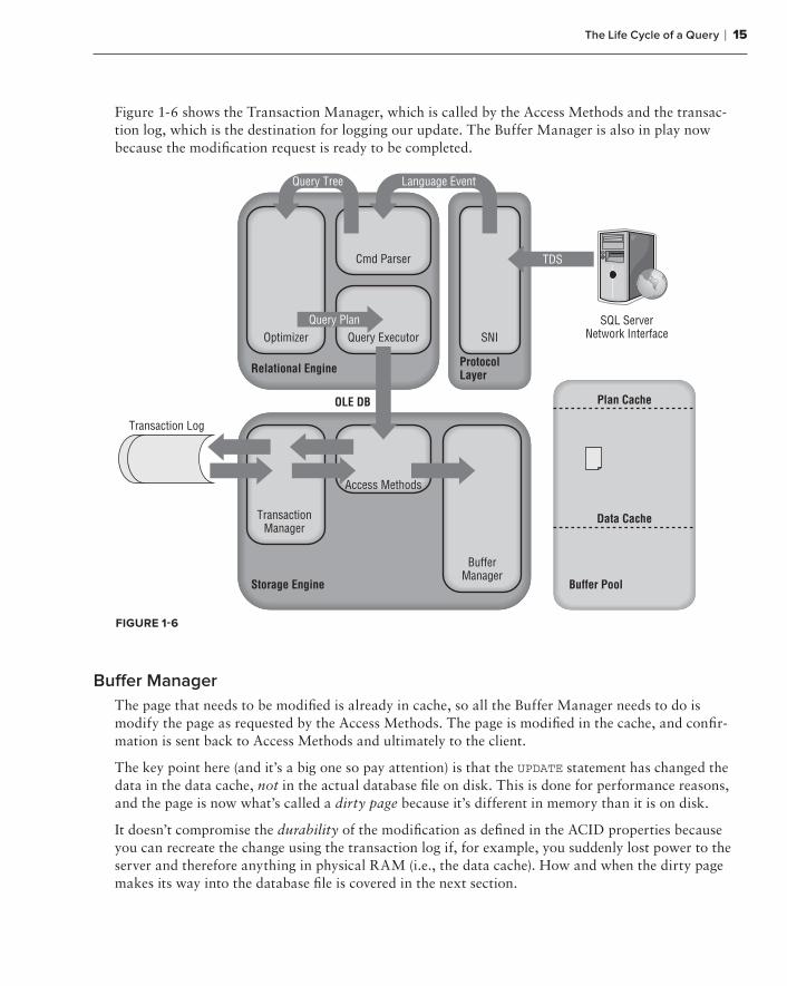
Figure 1-6 shows the Transaction Manager, which is called by the Access Methods and the transac-tion log, which is the destination for logging our update. The Buffer Manager is also in play now because the modifi cation request is ready to be completed.

Transaction Log

Cmd Parser

Query Executor

Access Methods

TransactionManager

BufferManager


Network Interface



Plan Cache

Data Cache

TDS

Query Plan


OLE DB

FIGURE 1-6

Buff er Manager

The page that needs to be modifi ed is already in cache, so all the Buffer Manager needs to do is modify the page as requested by the Access Methods. The page is modifi ed in the cache, and confi r-mation is sent back to Access Methods and ultimately to the client.

The key point here (and it’s a big one so pay attention) is that the UPDATE statement has changed the data in the data cache, not in the actual database fi le on disk. This is done for performance reasons, and the page is now what’s called a dirty page because it’s different in memory than it is on disk.

It doesn’t compromise the durability of the modifi cation as defi ned in the ACID properties because you can recreate the change using the transaction log if, for example, you suddenly lost power to the server and therefore anything in physical RAM (i.e., the data cache). How and when the dirty page makes its way into the database fi le is covered in the next section.

84289c01.indd 1584289c01.indd 15 11/23/09 4:11:24 PM11/23/09 4:11:24 PM


Figure 1-7 shows the completed life cycle for the update. The Buffer Manager has made the modi-fi cation to the page in cache and has passed confi rmation back up the chain. The database data fi le was not accessed during the operation, as you can see in the diagram.

Transaction Log

Cmd Parser

Query Executor

Access Methods

TransactionManager

BufferManager


Network Interface



Plan Cache

Data CacheData file

TDS

TDS

Query Plan


D

OLE DB

FIGURE 1-7

Recovery

In the previous section you read about the life cycle of an UPDATE query, which introduced Write-Ahead Logging as the method by which SQL Server maintains the durability of any changes.

Modifi cations are written to the transaction log fi rst and are then actioned in memory only. This is done for performance reasons and because you can recover the changes from the transaction log should you need to.

This process introduces some new concepts and terminology that are explored further in this section on “recovery.”

84289c01.indd 1684289c01.indd 16 11/23/09 4:11:25 PM11/23/09 4:11:25 PM


Dirty Pages

When a page is read from disk into memory it is regarded as a clean page because it’s exactly the same as its counterpart on the disk. However, once the page has been modifi ed in memory it is marked as a dirty page.

Clean pages can be fl ushed from cache using dbcc dropcleanbuffers, which can be handy when you’re troubleshooting development and test environments because it forces subsequent reads to be fulfi lled from disk, rather than cache, but doesn’t touch any dirty pages.

A dirty page is simply a page that has changed in memory since it was loaded from disk and is now different from the on-disk page. You can use the following query, which is based on the sys.dm_os_buffer_descriptors DMV, to see how many dirty pages exist in each database:

SELECT db_name(database_id) AS ‘Database’,count(page_id) AS ‘Dirty Pages’FROM sys.dm_os_buffer_descriptorsWHERE is_modified =1GROUP BY db_name(database_id)ORDER BY count(page_id) DESC

Running this on my test server produced the following results showing that at the time the query was run, there were just under 20MB (2,524*8\1,024) of dirty pages in the People database:

Database Dirty PagesPeople 2524Tempdb 61Master 1

These dirty pages will be written back to the database fi le periodically whenever the free buffer list is low or a checkpoint occurs. SQL Server always tries to maintain a number of free pages in cache in order to allocate pages quickly, and these free pages are tracked in the free buffer list.

Whenever a worker thread issues a read request, it gets a list of 64 pages in cache and checks whether the free buffer list is below a certain threshold. If it is, it will try to age-out some pages in its list, which causes any dirty pages to be written to disk.

Another thread called the lazywriter also works based on a low free buffer list.

Lazywriter

The lazywriter is a thread that periodically checks the size of the free buffer list. When it’s low, it scans the whole data cache to age-out any pages that haven’t been used for a while. If it fi nds any dirty pages that haven’t been used for a while, they are fl ushed to disk before being marked as free in memory.

The lazywriter also monitors the free physical memory on the server and will release memory from the free buffer list back to Windows in very low memory conditions. When SQL Server is busy, it will also grow the size of the free buffer list to meet demand (and therefore the buffer pool) when there is free physical memory and the confi gured Max Server Memory threshold hasn’t been reached. For more on Max Server Memory see Chapter 2.

84289c01.indd 1784289c01.indd 17 11/23/09 4:11:25 PM11/23/09 4:11:25 PM


Checkpoint Process

A checkpoint is a point in time created by the checkpoint process at which SQL Server can be sure that any committed transactions have had all their changes written to disk. This checkpoint then becomes the marker from which database recovery can start.

The checkpoint process ensures that any dirty pages associated with a committed transaction will be fl ushed to disk. Unlike the lazywriter, however, a checkpoint does not remove the page from cache; it makes sure the dirty page is written to disk and then marks the cached paged as clean in the page header.

By default, on a busy server, SQL Server will issue a checkpoint roughly every minute, which is marked in the transaction log. If the SQL Server instance or the database is restarted, then the recovery process reading the log knows that it doesn’t need to do anything with log records prior to the checkpoint.

The time between checkpoints therefore represents the amount of work that needs to be done to roll forward any committed transactions that occurred after the last checkpoint, and to roll back any transactions that hadn’t committed. By checkpointing every minute, SQL Server is trying to keep the recovery time when starting a database to less than one minute, but it won’t automatically check-point unless at least 10MB has been written to the log within the period.

Checkpoints can also be manually called by using the CHECKPOINT T-SQL command, and can occur because of other events happening in SQL Server. For example, when you issue a backup command, a checkpoint will run fi rst.

Trace fl ag 3502 is an undocumented trace fl ag that records in the error log when a checkpoint starts and stops. For example, after adding it as a startup trace fl ag and running a workload with numerous writes, my error log contained the entries shown in Figure 1-8, which indicates checkpoints running between 30 and 40 seconds apart.

ALL ABOUT TRACE FLAGS

Trace fl ags provide a way to change the behavior of SQL Server temporarily and are generally used to help with troubleshooting or for enabling and disabling certain features for testing. Hundreds of trace fl ags exist but very few are offi cially docu-mented; for a list of those that are and more information on using trace fl ags have a look here: http://msdn.microsoft.com/en-us/library/ms188396.aspx

FIGURE 1-8

84289c01.indd 1884289c01.indd 18 11/23/09 4:11:25 PM11/23/09 4:11:25 PM


Recovery Interval

Recovery Interval is a server confi guration option that can be used to infl uence the time between checkpoints, and therefore the time it takes to recover a database on startup — hence, “recovery interval.”

By default the recovery interval is set to 0, which allows SQL Server to choose an appropriate inter-val, which usually equates to roughly one minute between automatic checkpoints.

Changing this value to greater than 0 represents the number of minutes you want to allow between checkpoints. Under most circumstances you won’t need to change this value, but if you were more concerned about the overhead of the checkpoint process than the recovery time, you have the option.

However, the recovery interval is usually set only in test and lab environments where it’s set ridicu-lously high in order to effectively stop automatic checkpointing for the purpose of monitoring some-thing or to gain a performance advantage.

Unless you’re chasing world speed records for SQL Server you shouldn’t need to change it in a real-world production environment.

SQL Server evens throttles checkpoint I/O to stop it from impacting the disk subsystem too much, so it’s quite good at self-governing. If you ever see the SLEEP_BPOOL_FLUSH wait type on your server, that means checkpoint I/O was throttled to maintain overall system performance. You can read all about waits and wait types in Chapter 3.

Recovery Models

SQL Server has three database recovery models: Full, bulk-logged, and simple. Which model you choose affects the way the transaction log is used and how big it grows, your backup strategy, and your restore options.

Full

Databases using the full recovery model have all of their operations fully logged in the transaction log and must have a backup strategy that includes full backups and transaction log backups.

Starting with SQL Server 2005, Full backups don’t truncate the transaction log. This is so that the sequence of transaction log backups isn’t broken and gives you an extra recovery option if your full backup is damaged.

SQL Server databases that require the highest level of recoverability should use the Full Recovery Model.

Bulk-Logged

This is a special recovery model because it is intended to be used only temporarily to improve the performance of certain bulk operations by minimally-logging them; all other operations are fully-logged just like the full recovery model. This can improve performance because only the information required to roll back the transaction is logged. Redo information is not logged which means that you also lose point-in-time-recovery.

84289c01.indd 1984289c01.indd 19 11/23/09 4:11:25 PM11/23/09 4:11:25 PM


These bulk operations include:

BULK INSERT ➤

Using the bcp executable ➤

SELECT INTO ➤

CREATE INDEX ➤

ALTER INDEX REBUILD ➤

DROP INDEX ➤

Simple

When the simple recovery model is set on a database, all committed transactions are truncated from the transaction log every time a checkpoint occurs. This ensures that the size of the log is kept to a minimum and that transaction log backups are not necessary (or even possible). Whether or not that is a good or a bad thing depends on what level of recovery you require for the database.

If the potential to lose all the changes since the last full or differential backup still meets your busi-ness requirements then simple recovery might be the way to go.

THE SQLOS (SQL OPERATING SYSTEM)

So far, this chapter has abstracted the concept of the SQLOS to make the fl ow of components through the architecture easier to understand without going off on too many tangents. However, the SQLOS is core to SQL Server’s architecture so you need to understand why it exists and what it does to com-plete your view of how SQL Server works.

In summary, the SQLOS is a thin user-mode layer (Chapter 2) that sits between SQL Server and Windows. It is used for low-level operations such as scheduling, I/O completion, memory manage-ment, and resource management.

To explore exactly what this means and why it’s needed, you fi rst need to understand a bit about Windows.

Windows is a general purpose OS and is not optimized for server-based applications, SQL Server in particular. Instead, the goal for the Windows development team is to make sure that any application written by a wide-range of developers inside and outside Microsoft will work correctly and have good performance. Windows needs to work well for these broad scenarios so the dev teams are not going to do anything special that would be used in less than 1% of applications.

For example, the scheduling in Windows is very basic because things are done for the common cause. Optimizing the way that threads are chosen for execution is always going to be limited because of this broad performance goal but if an application does its own scheduling then there is more intelligence about who to choose next. For example, assigning some threads a higher priority or deciding that choosing one thread for execution will prevent other threads being blocked later on.

84289c01.indd 2084289c01.indd 20 11/23/09 4:11:25 PM11/23/09 4:11:25 PM

The SQLOS (SQL Operating System) ❘ 21

Scheduling is the method by which units of work are given time on a CPU to execute. See Chapter 5 for more information.

In a lot of cases SQL Server had custom code to handle a lot of these areas already. The User Mode Scheduler (UMS) was introduced in SQL Server 7 to handle scheduling and SQL Server was manag-ing its own memory even earlier than that.

The idea for SQLOS (which was fi rst implemented in SQL Server 2005) was to take all of these things developed by different internal SQL Server development teams to provide performance improvements on Windows and put them in a single place with a single team that will continue to optimize these low-level functions. This then leaves the other teams to concentrate on challenges more specifi c to their own domain within SQL Server.

DEFINING DMVS

Dynamic Management Views (DMVs) allow much greater visibility into the work-ings of SQL Server than in any version prior to SQL Server 2005. They are basi-cally just views on top of the system tables, but the concept allows Microsoft to provide a massive amount of useful information through them.

The standard syntax starts with sys.dm,_which indicates that it’s a DMV (there are also Dynamic Management Functions but DMV is still the collective term in popular use) followed by the area about which the DMV provides information, for example, sys.dm_os_for SQLOS, sys.dm_db_for database, and sys.dm_exec_for query execution.

The last part of the name describes the actual content accessible within the view; sys.dm_db_index_usage_stats and sys.dm_os_waiting_tasks are a couple of examples and you’ll come across many more throughout the book.

Another benefi t to having everything in one place is that you can now get better visibility of what’s happening at that level than was possible prior to SQLOS. You can access all this information through dynamic management views (DMVs). Any DMV that starts with sys.dm_os_ provides an insight into the workings of SQLOS. For example:

sys.dm_os_schedulers: ➤ Returns one row per scheduler (there is one user scheduler per core) and shows information on scheduler load and health. See Chapters 3 and 5 for more information.

sys.dm_os_waiting_tasks: ➤ Returns one row for every executing task that is currently waiting for a resource as well as the wait type. See Chapter 3 for more information.

sys.dm_os_memory_clerks: ➤ Memory clerks are used by SQL Server to allocate memory. Signifi cant components within SQL Server have their own memory clerk. This DMV shows all the memory clerks and how much memory each one is using. See Chapter 2 for more information.

84289c01.indd 2184289c01.indd 21 11/23/09 4:11:25 PM11/23/09 4:11:25 PM


Relating SQLOS back to the architecture diagrams seen earlier, many of the components will make calls to the SQLOS in order to fulfi ll low-level functions required to support their roles.

Just to be clear, the SQLOS doesn’t replace Windows. Ultimately, everything ends up using the documented Windows system services; SQL Server just uses them in such a way as to optimize for its own specifi c scenarios.

SQLOS is not a way to port the SQL Server architecture to other platforms like Linux or MacOS so it’s not an OS abstraction layer. It doesn’t wrap all the OS APIs like other frameworks such as .NET, which is why it’s referred to as a “thin” user-mode layer. Only the things that SQL Server really needs have been put into SQLOS.

SUMMARY

In this chapter you learned about SQL Server’s architecture by following the fl ow of components used when you issue a read request and an update request. You also learned some key terminology and processes used for the recovery of SQL Server databases and where the SQLOS fi ts into the architecture.

The key takeaways from this chapter are:

The Query Optimizer’s job is to fi nd a good plan in a reasonable amount of time; not the ➤

best plan.

Anything you want to read or update will need to be read into memory fi rst. ➤

Any updates to data will be written to the transaction log on disk before being updated in ➤

memory so transaction log performance is critical; the update isn’t written directly to the data fi le.

A database page that is changed in memory but not on disk is known as a dirty page. ➤

Dirty pages are fl ushed to disk by the checkpoint process and the lazywriter. ➤

Checkpoints occur automatically, roughly every minute and provide the starting point for ➤

recovery.

The lazywriter keeps space available in cache by fl ushing dirty pages to disk and keeping only ➤

recently used pages in cache.

When a database is using the Full recovery model, full backups will not truncate the transac- ➤

tion log. You must confi gure transaction log backups.

The SQLOS is a framework used by components in SQL Server for scheduling, I/O, and memory management.

84289c01.indd 2284289c01.indd 22 11/23/09 4:11:25 PM11/23/09 4:11:25 PM

Documents

SQL Server Architecture - Wiley · As shown in Figure 1-1, SQL Server is split into two main engines: the Relational Engine and the Storage Engine. The Relational Engine is also sometimes