SQL Server Performance Tuning

on Google Compute Engine

Erik Darling Brent Ozar Unlimited

March 2017

Table of contents Introduction

Measuring your existing SQL Server Trending backup size

Projecting future space requirements Trending backup speed

Bonus section: Backing up to NUL Trending DBCC CHECKDB Trending index maintenance Recap: your current vital stats

Sizing your Google Compute Engine VM Choosing your instance type

Compute Engine’s relationship between cores and memory Memory is more important in the cloud Choosing your CPU type

Putting it all together: build, then experiment

Measuring what SQL Server is waiting on An introduction to wait stats Getting more granular wait stats data Wait type reference list

CPU Memory Disk Locks Latches Misc Always On Availability Groups waits

Demo: Showing wait stats with a live workload About the database: orders About the workload

Measuring SQL Server with sp_BlitzFirst Baseline #1: Waiting on PAGEIOLATCH, CXPACKET, SOS_SCHEDULER_YIELD

Mitigation #1: Fixing PAGEIOLATCH, SOS_SCHEDULER_YIELD Configuring SQL Server to use the increased power TempDB

Moving TempDB Max server memory

1

CPU

Baseline #2: PAGEIOLATCH gone, SOS_SCHEDULER_YIELD still here Mitigation #2: Adding cores for SOS_SCHEDULER_YIELD waits

Baseline #3: High CPU, and now LCK* waits Mitigation #3: Fixing LCK* waits with optimistic isolation levels Batch requests per second

2

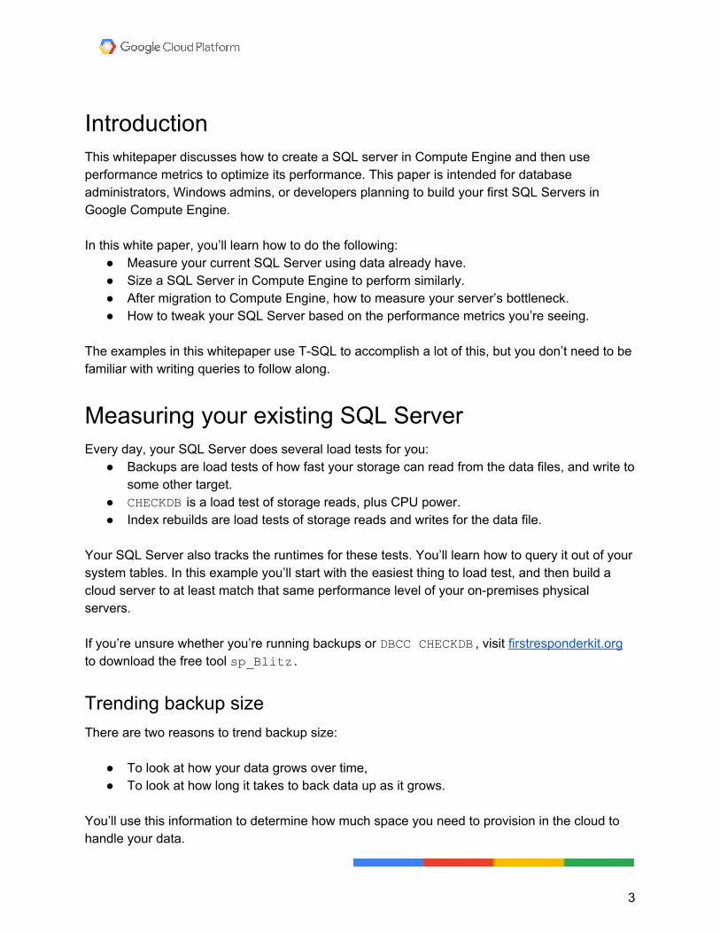
Introduction This whitepaper discusses how to create a SQL server in Compute Engine and then use performance metrics to optimize its performance. This paper is intended for database administrators, Windows admins, or developers planning to build your first SQL Servers in Google Compute Engine. In this white paper, you’ll learn how to do the following:

● Measure your current SQL Server using data already have. ● Size a SQL Server in Compute Engine to perform similarly. ● After migration to Compute Engine, how to measure your server’s bottleneck. ● How to tweak your SQL Server based on the performance metrics you’re seeing.

The examples in this whitepaper use T-SQL to accomplish a lot of this, but you don’t need to be familiar with writing queries to follow along.

Measuring your existing SQL Server Every day, your SQL Server does several load tests for you:

● Backups are load tests of how fast your storage can read from the data files, and write to some other target.

● CHECKDB is a load test of storage reads, plus CPU power. ● Index rebuilds are load tests of storage reads and writes for the data file.

Your SQL Server also tracks the runtimes for these tests. You’ll learn how to query it out of your system tables. In this example you’ll start with the easiest thing to load test, and then build a cloud server to at least match that same performance level of your on-premises physical servers. If you’re unsure whether you’re running backups or DBCC CHECKDB , visit firstresponderkit.org to download the free tool sp_Blitz .

Trending backup size There are two reasons to trend backup size:

● To look at how your data grows over time, ● To look at how long it takes to back data up as it grows.

You’ll use this information to determine how much space you need to provision in the cloud to handle your data.

3

Remember, you don’t just need enough disk space to hold your data and log files, you also need it to hold your backups. As data grows over time, you need more space to hold everything. Add into that any data retention policies, and you may find yourself needing more drive space than you first anticipated. You’ll walk through how to calculate how much space you’ll need after you review the scripts to collect different metrics. You’ll also consider how fast your current disks are, so you have a good idea about what you’ll need to provision elsewhere to get equivalent or better performance.

4

This query will get you backup sizes over the last year: SET TRANSACTION ISOLATION LEVEL READ UNCOMMITTED DECLARE @startDate DATETIME; SET @startDate = GETDATE(); SELECT PVT.DatabaseName ,

PVT.[0] , PVT.[-1] , PVT.[-2] , PVT.[-3] , PVT.[-4] , PVT.[-5] , PVT.[-6] , PVT.[-7] , PVT.[-8] , PVT.[-9] , PVT.[-10] , PVT.[-11] , PVT.[-12]

FROM ( SELECT BS.database_name AS DatabaseName ,

DATEDIFF(mm, @startDate, BS.backup_start_date) AS MonthsAgo , CONVERT(NUMERIC(10, 1), AVG(BF.file_size / 1048576.0)) AS

AvgSizeMB FROM msdb.dbo.backupset AS BS INNER JOIN msdb.dbo.backupfile AS BF

ON BS.backup_set_id = BF.backup_set_id WHERE NOT BS.database_name IN ( 'master', 'msdb', 'model', 'tempdb' )

AND BF.[file_type] = 'D' AND BS.type = 'D' AND BS.backup_start_date BETWEEN DATEADD(yy, -1, @startDate) AND

@startDate GROUP BY BS.database_name ,

DATEDIFF(mm, @startDate, BS.backup_start_date) ) AS BCKSTAT PIVOT ( SUM(BCKSTAT.AvgSizeMB) FOR BCKSTAT.MonthsAgo IN ( [0], [-1], [-2], [-3], [-4], [-5], [-6], [-7], [-8], [-9], [-10], [-11], [-12] ) ) AS PVT ORDER BY PVT.DatabaseName;

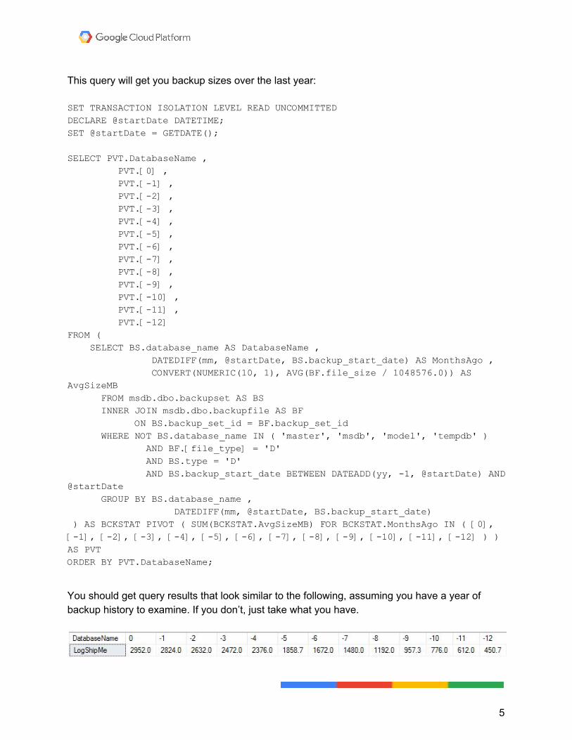
You should get query results that look similar to the following, assuming you have a year of backup history to examine. If you don’t, just take what you have.

5

This data trends easily because it uses a test database. The sample database grew by about 150 MB a month, resulting in a 3 GB database. This should help you figure out how much disk space you need to buy to account for your SQL data. For backups, you need to do a little extra math to account for data retention policies, and different backup types. For instance, if you have a policy to keep 2 weeks of data, you may be taking daily or weekly fulls, diffs at some more frequent interval (4/6/8 hours), and transaction logs at another interval (generally 60 minutes or less). You’ll need to look at current disk space usage for that data, and pad it upwards to account for data growth over time.

Projecting future space requirements Projecting space needed for, and growth of data backup files is not an exact science, and there are many factors to consider.

● Do you expect user counts to go up more than previously? (more users = more data) ● Do you expect to onboard more new clients than previously? ● Will you add new functionality to your application that will need to store additional data? ● Do you expect to onboard some number of large clients who are bringing a lot of

historical data? ● Are you changing your data retention periods? ● Are you going to start archiving/purging data?

If you’re expecting reasonably steady growth, you can just take your current backup space requirements and set up enough additional space to comfortably hold data one year from now. That looks something like current backups + current data * percent growth per month * 12 months. If you have 100 GB of backups and data, and a steady growth rate of 10% per month, you’ll need roughly 281 GB in a year. In two years, it’s nearly a terabyte. Padding the one year estimate up to 300 GB isn’t likely to have an appreciable impact on costs, but remember that with Compute Engine, storage, size, and performance are tied together. Larger disks have higher read and write speeds, up to a certain point. For less predictable rates, or special-circumstance rates, you’ll have to factor in further growth or reduction to suit your needs. For instance, if you have 5 years of data in your application, and you’re planning a one-time purge to reduce it to two years, then only keeping two years of live data online, you’ll want to start your calculation based on the size of two years of data.

6

You may be moving to the cloud because you’re expecting to onboard several large customers, and the up-front hardware/licensing costs, plus the costs of implementing more tolerant HA/DR to satisfy new SLAs, are too high. In some cases, clients will bring hundreds of gigs, possibly terabytes of historical data with them. Do your best to collect information about current size of data and data growth. If they’re already using SQL Server, you can send them the queries in this whitepaper to run so you have a good 1:1 comparison.

Trending backup speed The next thing to look at is how long backups take. Cutting out a chunk of the script above, you can trend that as well, along with the average MB-per-second backup throughput you’re getting. SET TRANSACTION ISOLATION LEVEL READ UNCOMMITTED DECLARE @startDate DATETIME; SET @startDate = GETDATE(); SELECT BS.database_name,

CONVERT(NUMERIC(10, 1), BF.file_size / 1048576.0) AS SizeMB, DATEDIFF(SECOND, BS.backup_start_date, BS.backup_finish_date) as

BackupSeconds, CAST(AVG(( BF.file_size / ( DATEDIFF(ss, BS.backup_start_date,

BS.backup_finish_date) ) / 1048576 )) AS INT) AS [Avg MB/Sec] FROM msdb.dbo.backupset AS BS

INNER JOIN msdb.dbo.backupfile AS BF ON BS.backup_set_id = BF.backup_set_id

WHERE NOT BS.database_name IN ( 'master', 'msdb', 'model', 'tempdb' ) AND BF.[file_type] = 'D' AND BS.type = 'D' AND BS.backup_start_date BETWEEN DATEADD(yy, -1, @startDate) AND

@startDate GROUP BY BS.database_name, CONVERT(NUMERIC(10, 1), BF.file_size / 1048576.0), DATEDIFF(SECOND, BS.backup_start_date, BS.backup_finish_date) ORDER BY CONVERT(NUMERIC(10, 1), BF.file_size / 1048576.0);

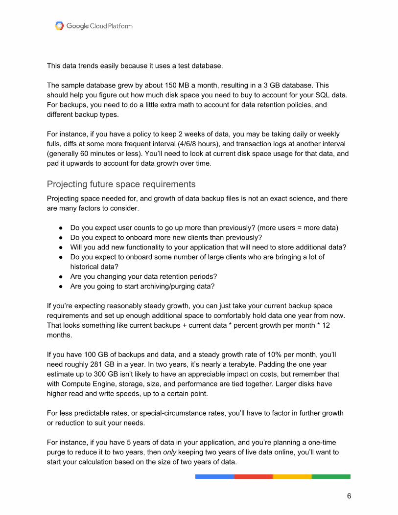
You should get results that look something like the following, assuming you have some backup history in msdb. This will tell you, for each database, how big it was in MB, how long the full backup took, and the average MB/sec.

7

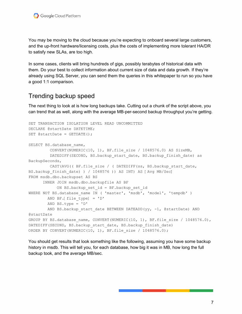
Keep in mind, this is a Compute Engine virtual machine (VM) with a 500 GB Standard Persisted disk, on a n1-standard-4 (4 CPUs, 15 GB memory). You're reading from and writing to the same drive, and this speed is terrible. On the next page is a reference chart of current transfer speeds. At the speeds we got, that’s subpar for even USB 2.0 connected storage. In the cloud, cheap disks aren’t good, and good disks aren’t cheap. Unless you provision local SSDs at startup, discussed later, speeds are around 250 MB/s for reads, and 100 MB/s for writes. That puts you somewhere in the neighborhood of 1 Gb iSCSI. Time to get started testing your local storage with a tool like Crystal Disk Mark or DiskSpd. If you’re already getting better speeds in your cloudless architecture, you need to know that going into a cloud implementation exercise, and how to mitigate where possible. If you’re getting lower or equivalent disk speeds, it’s time to start looking at how much it will cost to get similar performance in the cloud. All the potential savings in migrating to the cloud can quickly evaporate under the provisioning of many terabytes of cloud storage.

8

9

Backup time is important to test in the cloud. The time it takes to backup and restore data has implications for recovery point objectives (RPO) and recovery time objectives (RTO), as well as defined maintenance windows. When you get your database up in the cloud, take a backup and time it against current. Backup settings to consider:

● Compression ● Splitting the backup into multiple files ● Snapshot backups (with a third-party tool, if native backups aren’t fast enough)

Those settings can tune your number, and you may want to work on that first before going to the cloud. Otherwise, your big takeaway from this section: know your backup throughput in MB/sec.

Bonus section: Backing up to NUL To get a rough idea of how fast SQL can read data from disk during a backup, you can use a special command to backup to nowhere, or “backing up to NUL.” BACKUP DATABASE YourDatabase TO DISK = 'NUL' WITH COPY_ONLY

You will not get a backup from this, but you will know how fast you can read data from disk without the overhead of writing it to disk. Tip: Make sure to use the COPY_ONLY parameter, so the backup to nowhere doesn’t break your differential backup chain.

Trending DBCC CHECKDB You should check your databases for corruption with DBCC CHECKDB , either as a maintenance plan, or with trustworthy third-party tools, like Ola Hallengren’s free scripts, or MinionWare’s software. If you’ve been running DBCC CHECKDB through maintenance plans, you can get some rough idea of how long the process takes by looking at the job history. It may not be terribly valuable, unless CHECKDB is the only job step, and/or you have a separate job for each database. If you’ve been running DBCC CHECKDB with Ola Hallengren’s scripts, it’s easy to find out how long they take (as long as you’re logging the commands to a table -- which is the default). The following script takes the CommandLog table that Ola’s jobs populate as they run and joins them to backup information to obtain size data.

10

SET TRANSACTION ISOLATION LEVEL READ UNCOMMITTED DECLARE @startDate DATETIME; SET @startDate = GETDATE(); WITH cl AS (

SELECT DatabaseName, CommandType, StartTime, EndTime, DATEDIFF(SECOND, StartTime, EndTime) AS DBCC_Minutes

FROM master.dbo.CommandLog WHERE CommandType = 'DBCC_CHECKDB' AND NOT DatabaseName IN ( 'master', 'msdb', 'model', 'tempdb' )

) SELECT DISTINCT BS.database_name AS DatabaseName ,

CONVERT(NUMERIC(10, 1), BF.file_size / 1048576.0) AS SizeMB, cl.DBCC_Minutes, CAST( AVG(( BF.file_size / cl.DBCC_Minutes) / 1048576.0) AS INT) AS

[Avg MB/Sec] FROM msdb.dbo.backupset AS BS

INNER JOIN msdb.dbo.backupfile AS BF ON BS.backup_set_id = BF.backup_set_id

INNER JOIN cl ON cl.DatabaseName = BS.database_name

WHERE BF.[file_type] = 'D' AND BF.[file_type] = 'D' AND BS.type = 'D' AND BS.backup_start_date BETWEEN DATEADD(yy, -1, @startDate) AND

@startDate GROUP BY BS.database_name, CONVERT(NUMERIC(10, 1), BF.file_size / 1048576.0), cl.DBCC_Minutes;

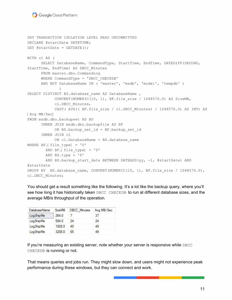
You should get a result something like the following. It’s a lot like the backup query, where you’ll see how long it has historically taken DBCC CHECKDB to run at different database sizes, and the average MB/s throughput of the operation.

If you’re measuring an existing server, note whether your server is responsive while DBCC CHECKDB is running or not. That means queries and jobs run. They might slow down, and users might not experience peak performance during these windows, but they can connect and work.

11

If your current server is responsive, then you have to make sure that your cloud hardware of choice holds up while maintenance is running. Just because it finishes in the same amount of time, with roughly the same throughput, doesn’t mean each server experiences load the same way. Have your app or some users ready to test connectivity during these processes. These are DBCC CHECKDB times on the same Compute Engine instance with a 500 GB persistent disk on a n1-standard-4 (4 CPUs, 15 GB memory). DBCC CHECKDB options to consider:

● Running PHYSICAL_ONLY checks ● Restoring full backups to another server to run CHECKDB (offloading) ● Running DBCC CHECKDB at different MAXDOP levels (2016+)

Trending index maintenance The same advice applies here as to the DBCC CHECKDB section: use either Ola’s or MinionWare’s scripts to do this. The problem with index maintenance is that you could have an unused index that gets fragmented because of modifications, and your maintenance routine will measure how fragmented it is, and then perform some action on it. This will not solve a single problem, but you’ll have expended a bunch of time and resources on it. No one really measures performance before and after, nor do they take into account the time and resources taken to perform the maintenance against any gains that may have occurred. For thresholds, we usually recommend 50% to reorganize, 80% to rebuild, and for larger databases, only tables with a page count > 5000. This is why it's good to just update stats. You give SQL updated information about what’s in your indexes and you invalidate old query plans. The updated statistics and invalidated plans are the best part or index rebuilds. Index reorgs don’t do either one.

12

Here’s an example using Ola’s CommandLog table again: WITH im AS (

SELECT DatabaseName, Command, StartTime, EndTime, DATEDIFF(SECOND, StartTime, EndTime) AS Index_Minutes, IndexName

FROM master.dbo.CommandLog WHERE CommandType LIKE '%INDEX%' AND NOT DatabaseName IN ( 'master', 'msdb', 'model', 'tempdb' )

) SELECT t.name, i.name AS IndexName, (SUM(a.used_pages) *8) / 1024. AS [Index MB],

MAX(im.Index_Minutes) AS WorldRecord, im.Command

FROM sys.indexes AS i JOIN sys.partitions AS p ON p.object_id = i.object_id AND p.index_id = i.index_id JOIN sys.allocation_units AS a

ON a.container_id = p.partition_id JOIN sys.tables t

ON t.object_id = i.object_id JOIN im

ON im.IndexName = i.name WHERE t.is_ms_shipped = 0 GROUP BY t.name, i.name, im.Command ORDER BY t.name, i.name;

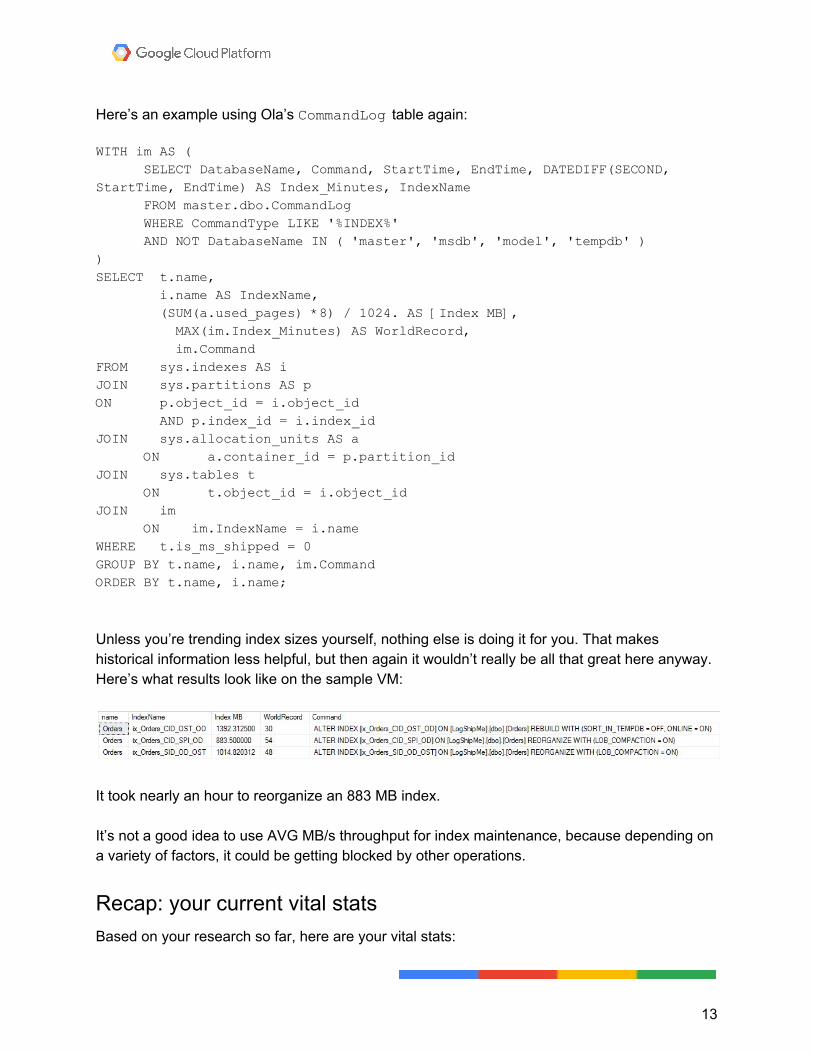
Unless you’re trending index sizes yourself, nothing else is doing it for you. That makes historical information less helpful, but then again it wouldn’t really be all that great here anyway. Here’s what results look like on the sample VM:

It took nearly an hour to reorganize an 883 MB index. It’s not a good idea to use AVG MB/s throughput for index maintenance, because depending on a variety of factors, it could be getting blocked by other operations.

Recap: your current vital stats Based on your research so far, here are your vital stats:

13

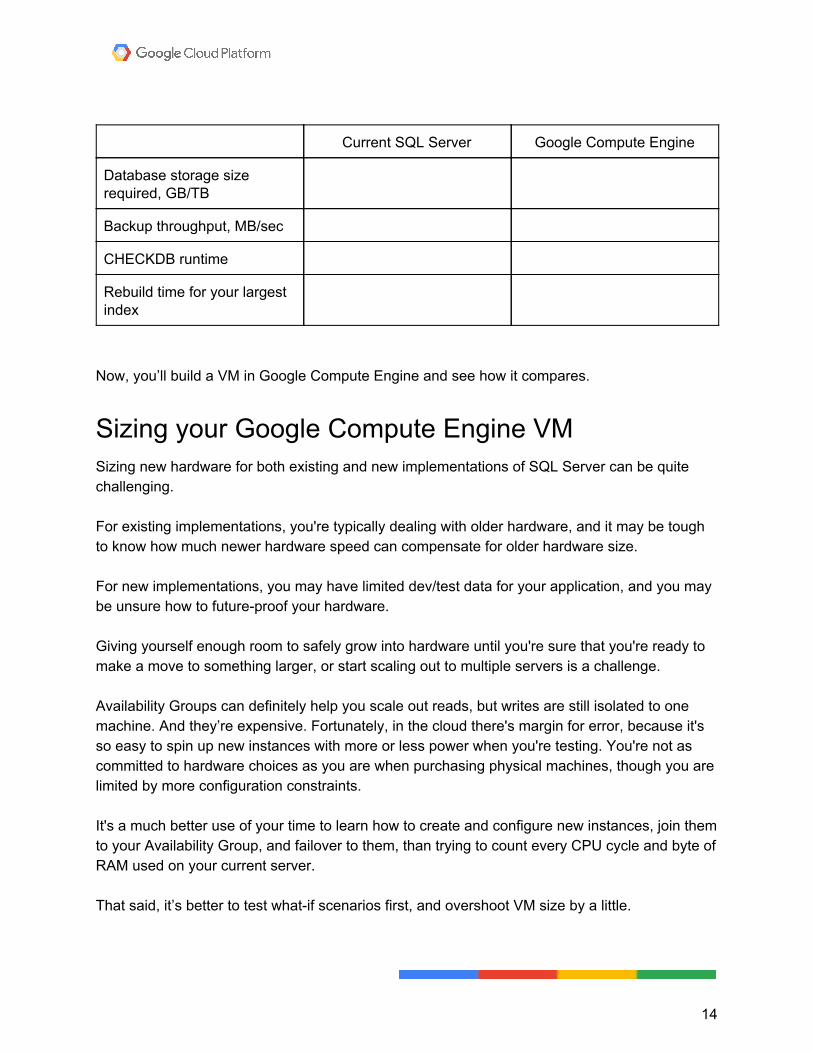
Current SQL Server Google Compute Engine

Database storage size required, GB/TB

Backup throughput, MB/sec

CHECKDB runtime

Rebuild time for your largest index

Now, you’ll build a VM in Google Compute Engine and see how it compares.

Sizing your Google Compute Engine VM Sizing new hardware for both existing and new implementations of SQL Server can be quite challenging. For existing implementations, you're typically dealing with older hardware, and it may be tough to know how much newer hardware speed can compensate for older hardware size. For new implementations, you may have limited dev/test data for your application, and you may be unsure how to future-proof your hardware. Giving yourself enough room to safely grow into hardware until you're sure that you're ready to make a move to something larger, or start scaling out to multiple servers is a challenge. Availability Groups can definitely help you scale out reads, but writes are still isolated to one machine. And they’re expensive. Fortunately, in the cloud there's margin for error, because it's so easy to spin up new instances with more or less power when you're testing. You're not as committed to hardware choices as you are when purchasing physical machines, though you are limited by more configuration constraints. It's a much better use of your time to learn how to create and configure new instances, join them to your Availability Group, and failover to them, than trying to count every CPU cycle and byte of RAM used on your current server. That said, it’s better to test what-if scenarios first, and overshoot VM size by a little.

14

Choosing your instance type First, you pick which instance type you want, and then you’ll configure the instance type with your exact CPU/memory/storage requirements.

Compute Engine’s relationship between cores and memory If you’ve built virtual machines before (either on-premises or in other cloud providers), you’re used to picking whatever core count you want, and whatever memory amount you want. Those two numbers haven’t had a relationship -- until now. Google Compute Engine is different because the memory amount is a direct relationship to the CPU core count:

● standard machines have 3.75 GB RAM per CPU ● highcpu machine have 0.9 GB RAM per CPU ● highmem machines have 6.5 GB RAM per CPU

That means when you hit 32 cores, your RAM is capped at 120 GB, 28.8 GB, and 208 GB, respectively. (Note that for custom VMs, your CPU and RAM max out at 32 CPUs and 208 GB RAM, just like highmem). .9GB per CPU isn’t enough for SQL Server, unless your current workload is CPU bound, with fewer cores and commensurate RAM. When you choose a Compute Engine instance to run SQL Server, the machine types that make the most sense are from the highmem, standard, or custom family. They offer more RAM per CPU than the highcpu family. Looking at the following chart, it’s easy to see why the highcpu machine types are unlikely to suit your workload, though, ironically, it’s highest level configuration is just about what your workload will need in this example (you’ll actually have 40 GB RAM, which is slightly higher), because your database is only around 20 GB. You just wouldn’t want to rely on that in the real world, with real data, that will likely grow much faster than this test data, which is just one table in a database with a limited number of indexes on it. A real workload with multiple tables that need to be indexed and joined and reported on, will look different. Understanding your working data set is important to sizing your VM. You could have a 100 GB database that only has 40 GB of data that users access regularly. Most workloads, especially those that will be using Availability Groups, should begin testing at one of the higher CPU count instance types listed in the chart.

15

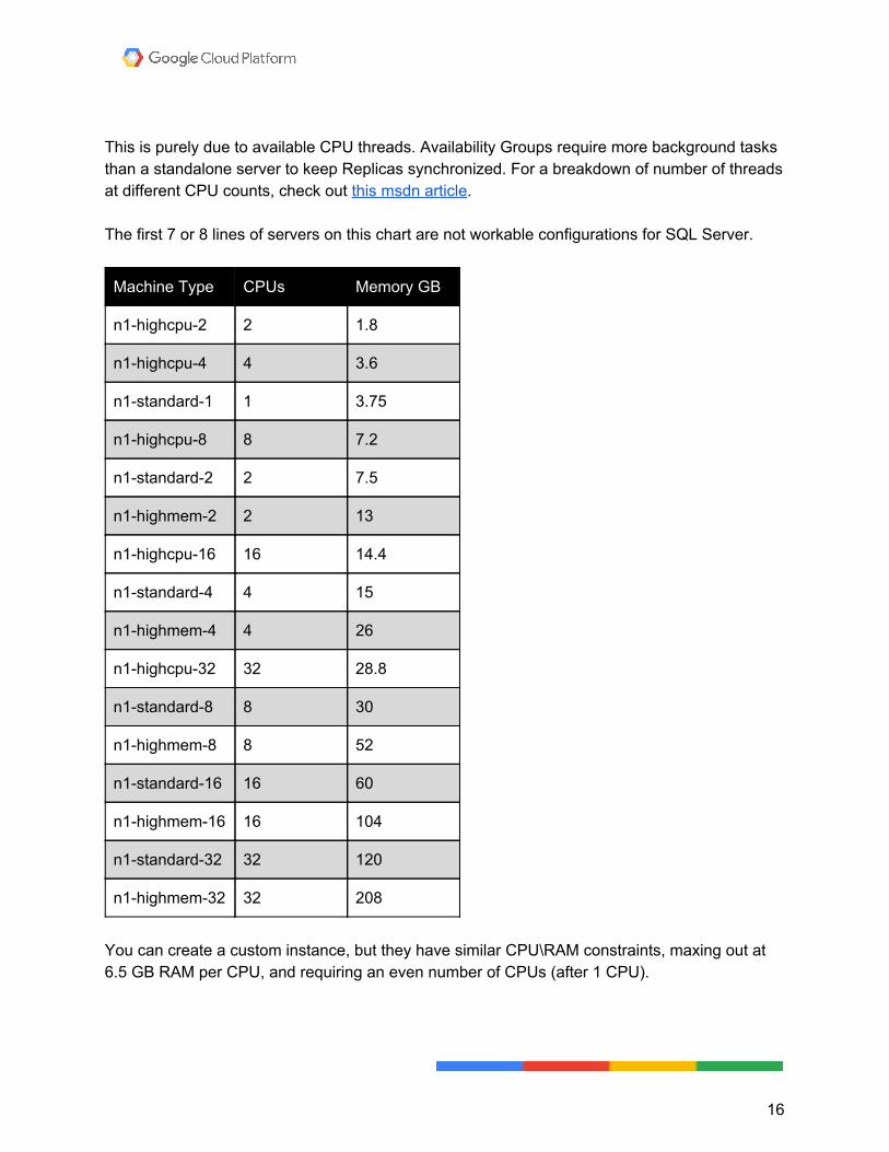
This is purely due to available CPU threads. Availability Groups require more background tasks than a standalone server to keep Replicas synchronized. For a breakdown of number of threads at different CPU counts, check out this msdn article. The first 7 or 8 lines of servers on this chart are not workable configurations for SQL Server.

Machine Type CPUs Memory GB

n1-highcpu-2 2 1.8

n1-highcpu-4 4 3.6

n1-standard-1 1 3.75

n1-highcpu-8 8 7.2

n1-standard-2 2 7.5

n1-highmem-2 2 13

n1-highcpu-16 16 14.4

n1-standard-4 4 15

n1-highmem-4 4 26

n1-highcpu-32 32 28.8

n1-standard-8 8 30

n1-highmem-8 8 52

n1-standard-16 16 60

n1-highmem-16 16 104

n1-standard-32 32 120

n1-highmem-32 32 208

You can create a custom instance, but they have similar CPU\RAM constraints, maxing out at 6.5 GB RAM per CPU, and requiring an even number of CPUs (after 1 CPU).

16

Examples of CPU and RAM limits for custom instances are as follows:

● 4 CPUs : 26 GB RAM ● 6 CPUs : 39 GB RAM ● 8 CPUs : 52 GB RAM ● 10 CPUS : 65 GB RAM ● 12 CPUs : 78 GB RAM ● 16 CPUs : 104 GB RAM ● 20 CPUs : 130 GB RAM ● 24 CPUs : 156 GB RAM ● 32 CPUs : 208 GB RAM

These configs are common real-world scenarios. There are even-number CPU steps in between some of these, but this should illustrate the relationship between CPU count and RAM limits in customized instances.

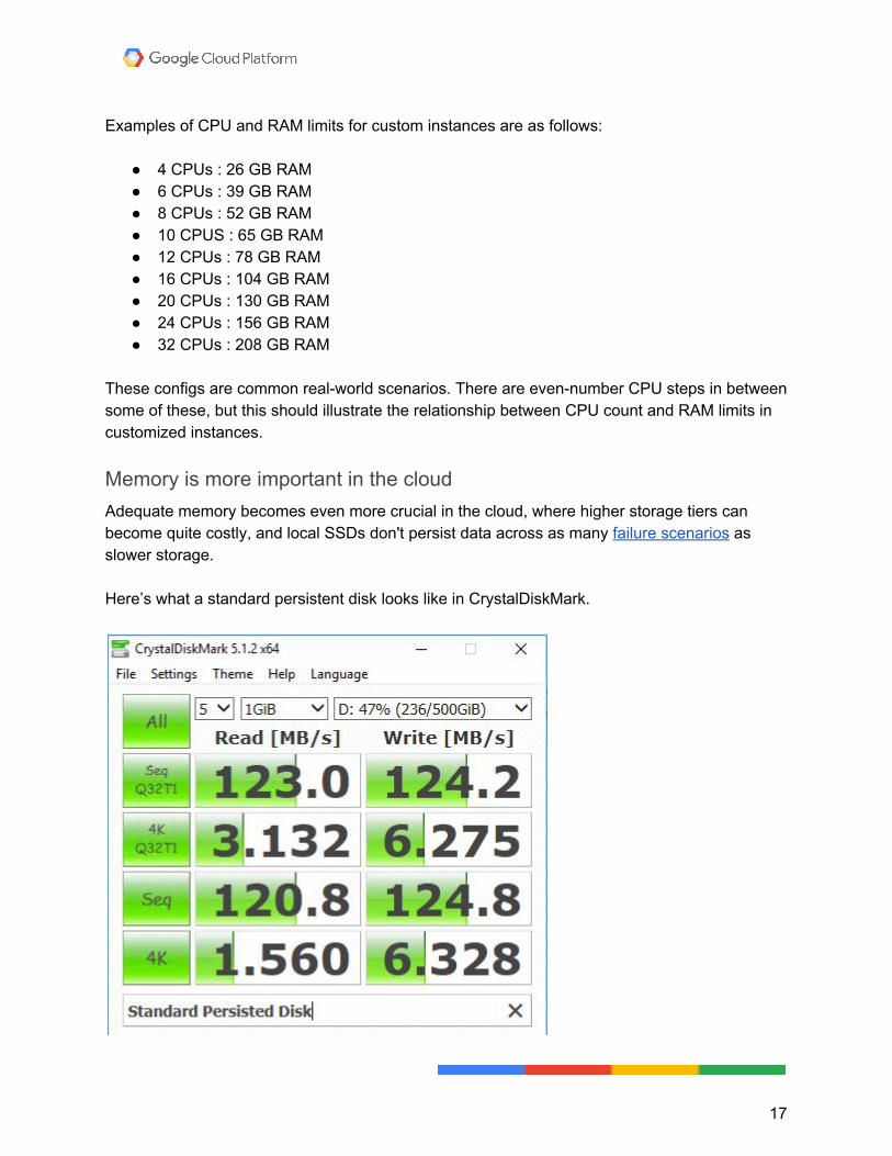
Memory is more important in the cloud Adequate memory becomes even more crucial in the cloud, where higher storage tiers can become quite costly, and local SSDs don't persist data across as many failure scenarios as slower storage. Here’s what a standard persistent disk looks like in CrystalDiskMark.

17

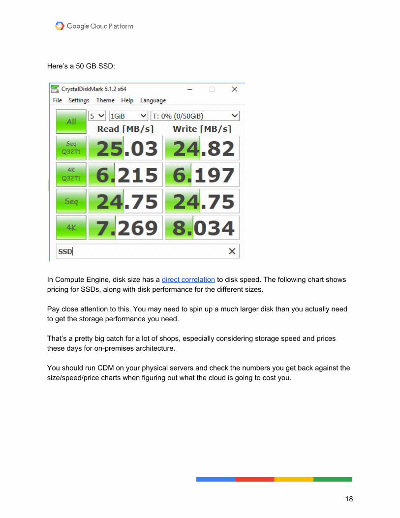
Here’s a 50 GB SSD:

In Compute Engine, disk size has a direct correlation to disk speed. The following chart shows pricing for SSDs, along with disk performance for the different sizes. Pay close attention to this. You may need to spin up a much larger disk than you actually need to get the storage performance you need. That’s a pretty big catch for a lot of shops, especially considering storage speed and prices these days for on-premises architecture. You should run CDM on your physical servers and check the numbers you get back against the size/speed/price charts when figuring out what the cloud is going to cost you.

18

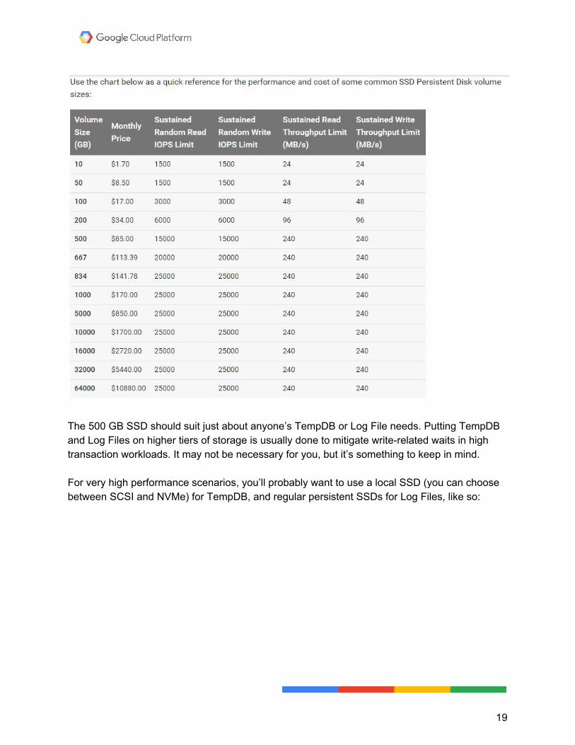
The 500 GB SSD should suit just about anyone’s TempDB or Log File needs. Putting TempDB and Log Files on higher tiers of storage is usually done to mitigate write-related waits in high transaction workloads. It may not be necessary for you, but it’s something to keep in mind. For very high performance scenarios, you’ll probably want to use a local SSD (you can choose between SCSI and NVMe) for TempDB, and regular persistent SSDs for Log Files, like so:

19

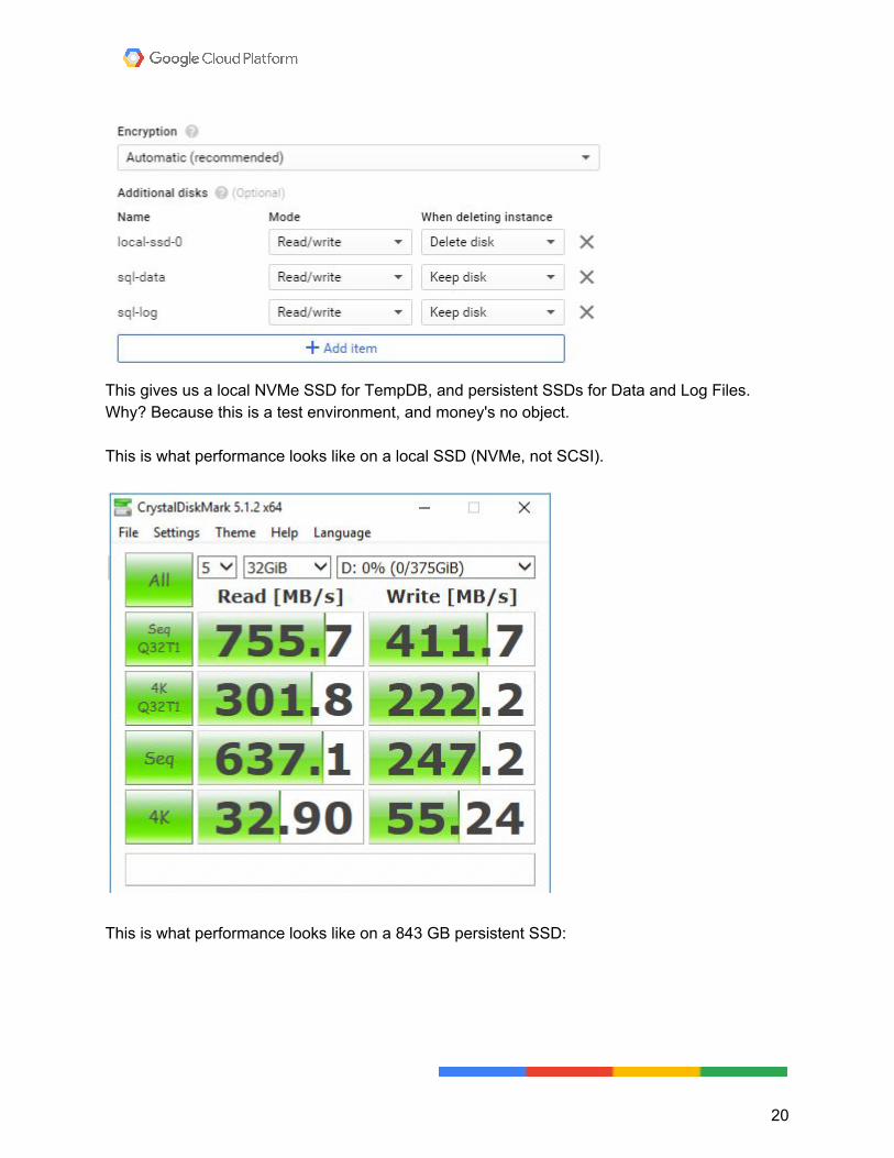
This gives us a local NVMe SSD for TempDB, and persistent SSDs for Data and Log Files. Why? Because this is a test environment, and money's no object. This is what performance looks like on a local SSD (NVMe, not SCSI).

This is what performance looks like on a 843 GB persistent SSD:

20

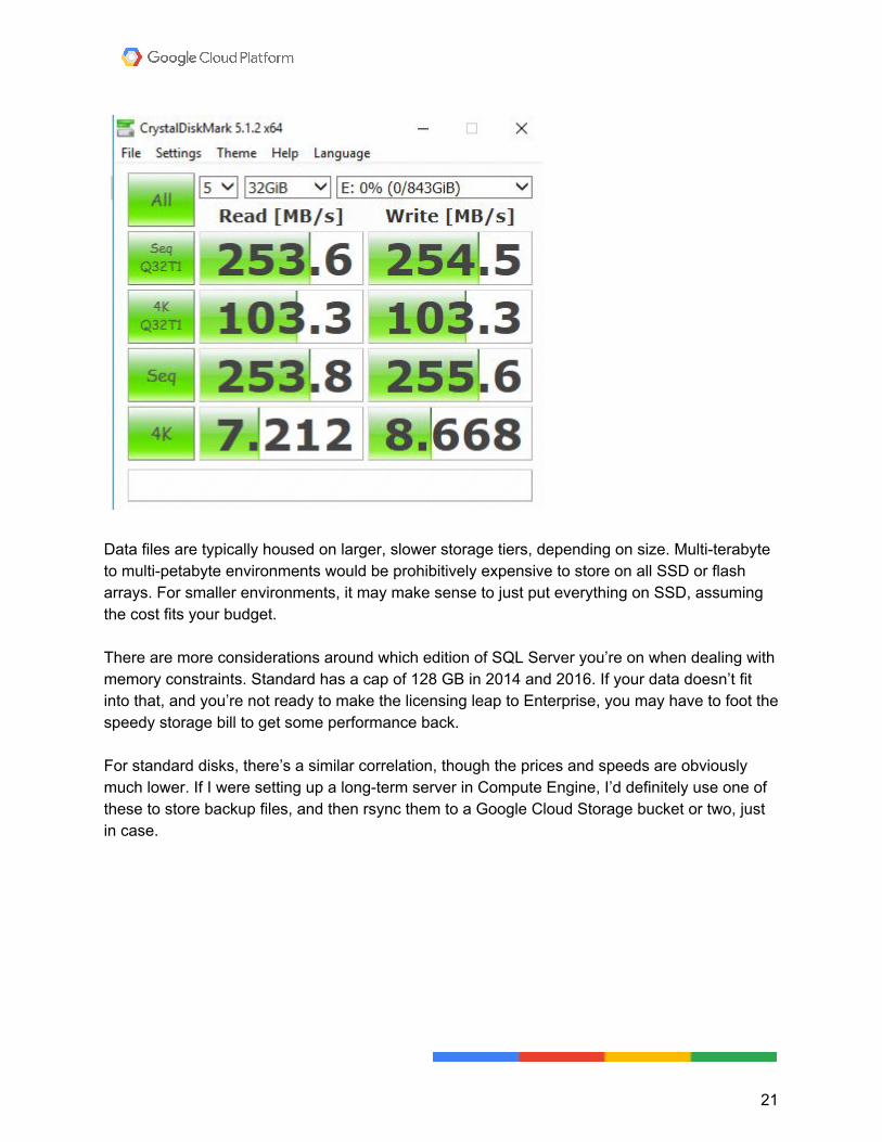
Data files are typically housed on larger, slower storage tiers, depending on size. Multi-terabyte to multi-petabyte environments would be prohibitively expensive to store on all SSD or flash arrays. For smaller environments, it may make sense to just put everything on SSD, assuming the cost fits your budget. There are more considerations around which edition of SQL Server you’re on when dealing with memory constraints. Standard has a cap of 128 GB in 2014 and 2016. If your data doesn’t fit into that, and you’re not ready to make the licensing leap to Enterprise, you may have to foot the speedy storage bill to get some performance back. For standard disks, there’s a similar correlation, though the prices and speeds are obviously much lower. If I were setting up a long-term server in Compute Engine, I’d definitely use one of these to store backup files, and then rsync them to a Google Cloud Storage bucket or two, just in case.

21

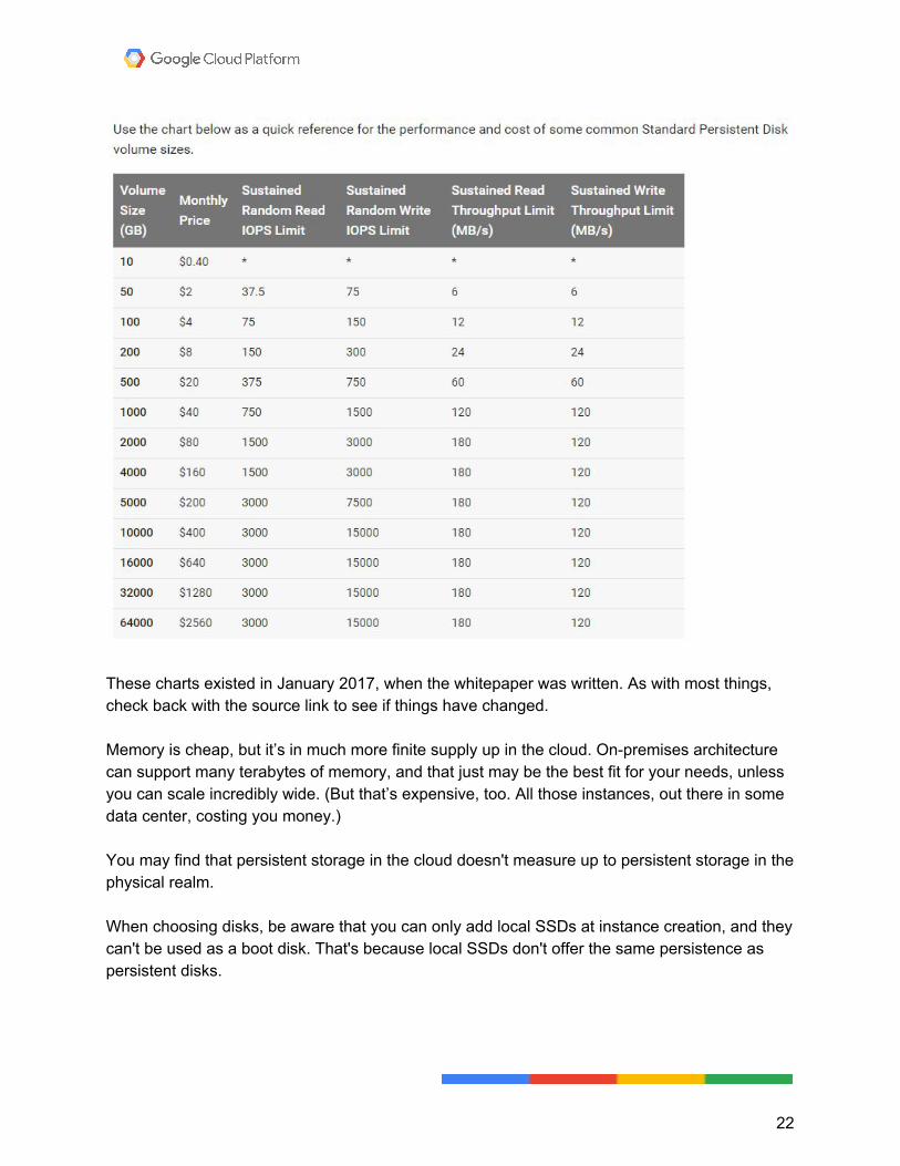
These charts existed in January 2017, when the whitepaper was written. As with most things, check back with the source link to see if things have changed. Memory is cheap, but it’s in much more finite supply up in the cloud. On-premises architecture can support many terabytes of memory, and that just may be the best fit for your needs, unless you can scale incredibly wide. (But that’s expensive, too. All those instances, out there in some data center, costing you money.) You may find that persistent storage in the cloud doesn't measure up to persistent storage in the physical realm. When choosing disks, be aware that you can only add local SSDs at instance creation, and they can't be used as a boot disk. That's because local SSDs don't offer the same persistence as persistent disks.

22

Data can be lost, so it may only make sense to have something like TempDB on them, since it's reinitialized when SQL starts up anyway. Local SSDs can hang onto data under certain circumstances, like rebooting the guest, or if the instance is set up for live migration. There is an option for SSD persistent disks, which are governed by the size/speed/price chart in the previous section. These can be booted from, and added at any time, but cost much more than standard persistent disks. They’re fast, but slower than their local SSD counterparts.

Choosing your CPU type CPU is another important consideration. As of this writing, the CPU types available are:

● 2.6 GHz Intel Xeon E5 (Sandy Bridge) ● 2.5 GHz Intel Xeon E5 v2 (Ivy Bridge) ● 2.3 GHz Intel Xeon E5 v3 (Haswell) ● 2.2 GHz Intel Xeon E5 v4 (Broadwell)

Note that 32-core machine types are not available in Sandy Bridge zones us-central1-a and europe-west1-b. Careful comparison to current CPUs is in order -- if your CPUs have higher clock speeds, you may need to invest in more cores to get similar performance. You also don't get to choose which CPUs you get, so be prepared to assume you're getting the lowest clock speed, 2.2 GHz, when comparing to your current server build.

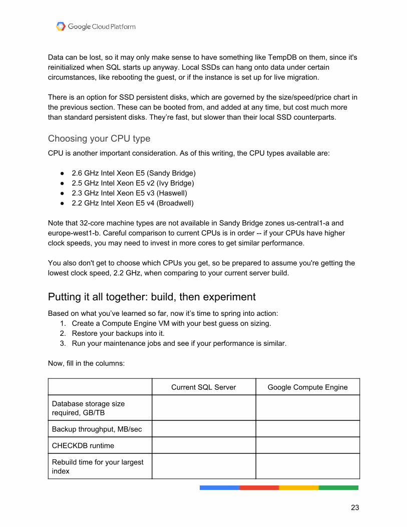
Putting it all together: build, then experiment Based on what you’ve learned so far, now it’s time to spring into action:

1. Create a Compute Engine VM with your best guess on sizing. 2. Restore your backups into it. 3. Run your maintenance jobs and see if your performance is similar.

Now, fill in the columns:

Current SQL Server Google Compute Engine

Database storage size required, GB/TB

Backup throughput, MB/sec

CHECKDB runtime

Rebuild time for your largest index

23

If you’re not satisfied with your performance metrics, you have two choices.

● You can do performance tuning. You can tune SQL Server’s maintenance jobs. For example, with SQL Server 2016, you can now pass a MAXDOP hint to the CHECKDB command to make it use more or less CPU cores. (This is beyond the scope of this paper).

● You can try a different instance size. To determine what that should be, you need to know what your bottleneck is.

Measuring what SQL Server is waiting on You're going to use wait statistics using an open source tool called sp_BlitzFirst. It’ll answer the following questions:

● Are there any current bottlenecks? ● What are things historically waiting on? ● What are queries currently waiting on?

An introduction to wait stats When a task runs in SQL Server, it has three potential states: running, runnable, and suspended.

● Running: Task is actively processing. ● Runnable: Task can run when it gets on a CPU. ● Suspended: Task is waiting on a resource or request to complete.

During each of these phases, the task may need to wait for a physical resource, like CPU, I/O, or memory. It may also need to wait on a logical resource, like a lock or latch on data pages already in memory. SQL Server tracks this data and exposes it to you in a dynamic management view (DMV) named sys.dm_os_wait_stats , but that’s painful to query because it just tracks cumulative time. You need more granular data -- you need to know exactly what SQL Server was waiting on, and more importantly, when . You don’t care that SQL Server was waiting on slow storage while your backups were running -- you care what it’s waiting on when your users are running their queries.

24

Getting more granular wait stats data There’s no replacement for a mature, platform-specific monitoring tool. Vendors we like include SentryOne, Quest, and Idera. For this whitepaper, you're going to use stored procedures from our First Responder Kit. Primarily, sp_BlitzFirst , which calls another stored procedure called sp_BlitzWho . sp_BlitzWho is an open source query similar to, but far less robust, than sp_WhoIsActive . It just shows you what’s running without many of the bells and whistles in sp_WhoIsActive . Whether you’re using a third party tool or an open source script like sp_BlitzFirst , you’re going to see a list of wait types.

Wait type reference list SQL Server has a robust array of wait types to indicate which resources tasks most frequently wait on. This paper focuses on the most common, and which resources they map to. They can lead you to your worst performance problems, and they can also tell you if your SQL Server is just sitting around. This list is by no means exhaustive. If you need information about a wait type not listed here, Waitopedia can be helpful. For more detailed help, the DBA Stack Exchange site is great for asking long-form questions.

CPU CXPACKET: Parallel queries running. This is neither good or bad. SOS_SCHEDULER_YIELD: Queries quietly queueing cooperatively. EXECSYNC: Parallel queries waiting on an operator to build an object (spool, etc.). THREADPOOL: Running out of CPU threads to run tasks with. This can be a sign of a big problem.

Memory RESOURCE_SEMAPHORE: Queries can’t get enough memory to run, so they wait. RESOURCE_SEMAPHORE_QUERY_COMPILE: Queries can’t get enough memory to compile a plan. Both resource semaphore wait types can be a sign of a pretty big problem. CMEMTHREAD: CPU threads trying to latch onto memory. This happens more often on systems with >8 cores per socket.

25

Disk PAGEIOLATCH_SH: These are all pages being read from disk into memory. PAGEIOLATCH_UP: If you have a lot of these waits, pay close attention to your cloud VM. PAGEIOLATCH_EX: It may need a lot more memory than your on-premises server has. Note that there are several other variety of PAGEIOLATCH_** waits, but they’re far less common. WRITELOG: SQL writing to log files.

Locks LCK_M_**: There are many, many variations of lock waits. They all start with LCK_M_ and then an acronym to designate the type of lock, etc. Diving into each one is beyond the scope of this whitepaper.

Latches LATCH_EX: Latches waiting for access to objects that aren’t data pages, already in memory. PAGELATCH_SH: Don’t confuse these with PAGEIOLATCH. The names look alike. PAGELATCH_UP: These are usually associated with objects in tempdb, but can also happenin regular user databases as well. PAGELATCH_EX: Note that there are several other variety of PAGELATCH_** waits, but they’re far less common.

Misc OLEDB: Most common during CHECKDB and Linked Server queries. BACKUP*: There are several wait types that start with BACKUP , which, along with ASYNC_IO_COMPLETION, accumulate during backups.

Always On Availability Groups waits If you implement an Availability Group, a number of other waits that may crop up, especially during data modifications. Using SQL Server 2016 is especially important for highly transactional workloads that are part of an Availability Group, because of the ability to REDO in parallel. It’s not just the SQL Server at work here, though. You have to push data across a network, and to another disk. Depending on which zone each node is in, and how far apart those zones are, you may have very different network performance, making synchronizing data difficult depending on the size of and volume of transactions.

26

You need to keep Replicas synchronous only in the same zone, and asynchronous otherwise.

27

Demo: Showing wait stats with a live workload You're starting off using the n1-standard-4 (4 CPUs, 15 GB memory) instance type. You have two standard persistent disks: one for the OS, and one for SQL that contains SQL Server binaries, Data, Log, TempDB, and backup files. Running SQL Server 2016, the only settings adjustments made are for memory and parallelism.

● Max server memory is set to 10 GB (10240 MB). ● MAXDOP is set to 4. ● Cost Threshold For Parallelism is set to 50.

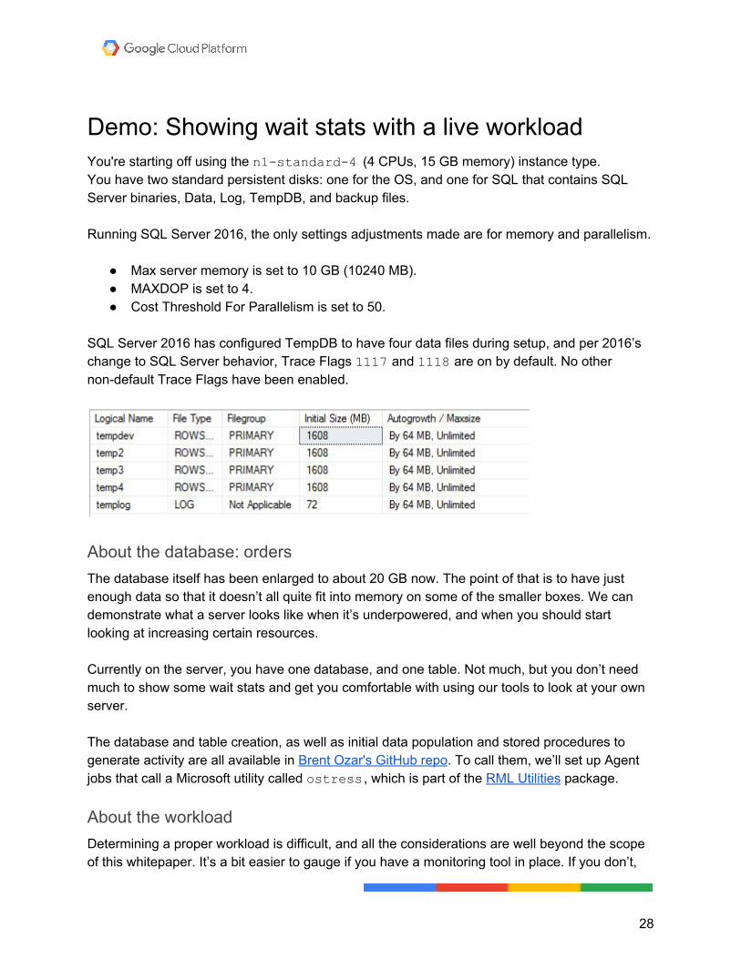
SQL Server 2016 has configured TempDB to have four data files during setup, and per 2016’s change to SQL Server behavior, Trace Flags 1117 and 1118 are on by default. No other non-default Trace Flags have been enabled.

About the database: orders The database itself has been enlarged to about 20 GB now. The point of that is to have just enough data so that it doesn’t all quite fit into memory on some of the smaller boxes. We can demonstrate what a server looks like when it’s underpowered, and when you should start looking at increasing certain resources. Currently on the server, you have one database, and one table. Not much, but you don’t need much to show some wait stats and get you comfortable with using our tools to look at your own server. The database and table creation, as well as initial data population and stored procedures to generate activity are all available in Brent Ozar's GitHub repo. To call them, we’ll set up Agent jobs that call a Microsoft utility called ostress , which is part of the RML Utilities package.

About the workload Determining a proper workload is difficult, and all the considerations are well beyond the scope of this whitepaper. It’s a bit easier to gauge if you have a monitoring tool in place. If you don’t,

28

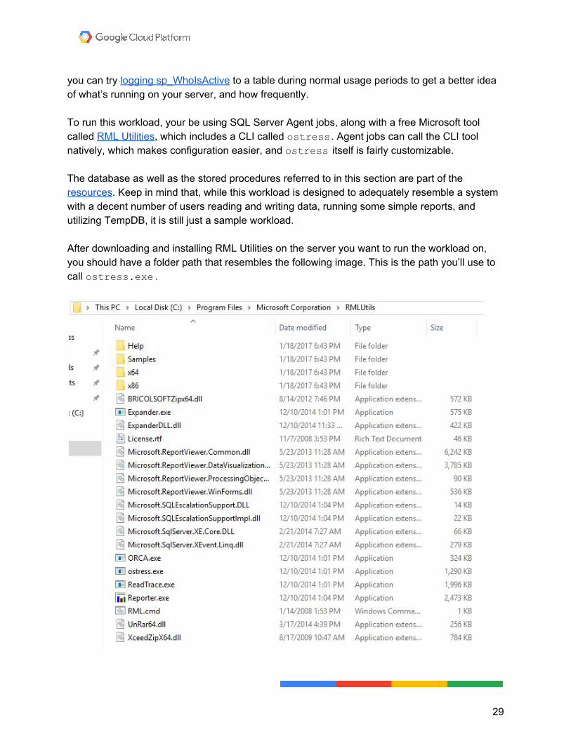
you can try logging sp_WhoIsActive to a table during normal usage periods to get a better idea of what’s running on your server, and how frequently. To run this workload, your be using SQL Server Agent jobs, along with a free Microsoft tool called RML Utilities, which includes a CLI called ostress . Agent jobs can call the CLI tool natively, which makes configuration easier, and ostress itself is fairly customizable. The database as well as the stored procedures referred to in this section are part of the resources. Keep in mind that, while this workload is designed to adequately resemble a system with a decent number of users reading and writing data, running some simple reports, and utilizing TempDB, it is still just a sample workload. After downloading and installing RML Utilities on the server you want to run the workload on, you should have a folder path that resembles the following image. This is the path you’ll use to call ostress.exe .

29

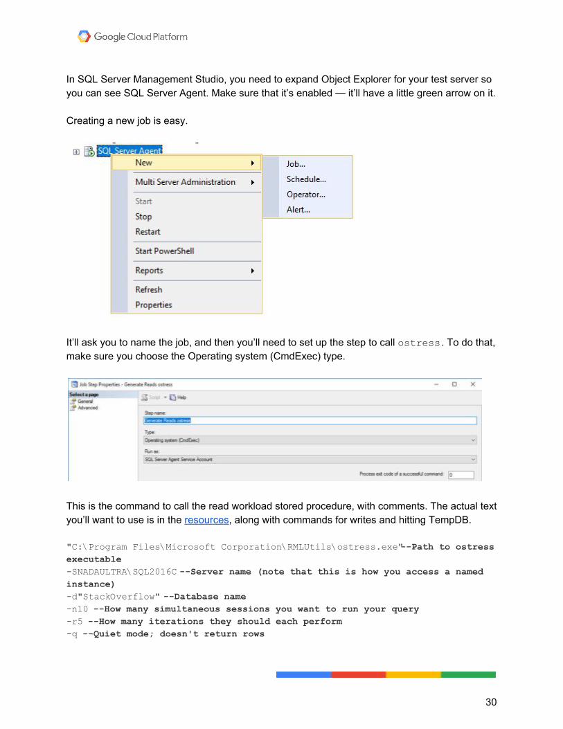
In SQL Server Management Studio, you need to expand Object Explorer for your test server so you can see SQL Server Agent. Make sure that it’s enabled — it’ll have a little green arrow on it. Creating a new job is easy.

It’ll ask you to name the job, and then you’ll need to set up the step to call ostress . To do that, make sure you choose the Operating system (CmdExec) type.

This is the command to call the read workload stored procedure, with comments. The actual text you’ll want to use is in the resources, along with commands for writes and hitting TempDB. "C:\Program Files\Microsoft Corporation\RMLUtils\ostress.exe" --Path to ostress executable -SNADAULTRA\SQL2016C --Server name (note that this is how you access a named instance) -d"StackOverflow" --Database name -n10 --How many simultaneous sessions you want to run your query -r5 --How many iterations they should each perform -q --Quiet mode; doesn't return rows

30

-Q"EXEC dbo.GenerateReads" --Query you want to run -o"C:\temp\readslog" --Logging folder

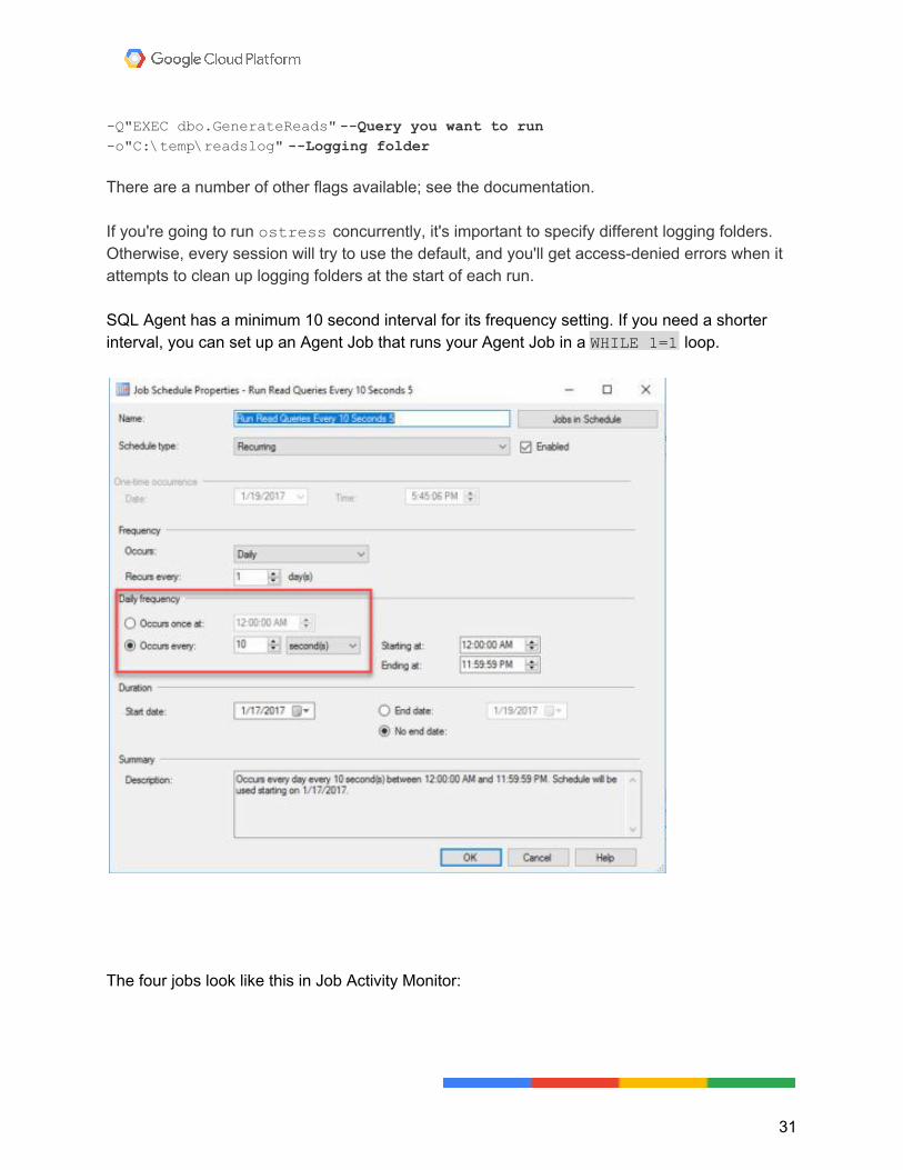
There are a number of other flags available; see the documentation. If you're going to run ostress concurrently, it's important to specify different logging folders. Otherwise, every session will try to use the default, and you'll get access-denied errors when it attempts to clean up logging folders at the start of each run. SQL Agent has a minimum 10 second interval for its frequency setting. If you need a shorter interval, you can set up an Agent Job that runs your Agent Job in a WHILE 1=1 loop.

The four jobs look like this in Job Activity Monitor:

31

Measuring SQL Server with sp_BlitzFirst You can run sp_BlitzFirst to see statistics since the server started up: EXEC sp_BlitzFirst @SinceStartup = 1

You can also take a current sample: EXEC sp_BlitzFirst @Seconds = 30, @ExpertMode = 1

These two options are sufficient for this demonstration. There are more options, detailed at firstresponderkit.org. Have a look at the wait stats.

Baseline #1: Waiting on PAGEIOLATCH, CXPACKET, SOS_SCHEDULER_YIELD

Since startup, you should have many waits. When looking at this, what should jump out isn’t just the total wait time, though that does indicate heavy resource usage, but also how efficient that resource is. Leaving aside the LCK_* waits, which indicate a locking problem, the top waits are all CPU and disk related. Neither resource is responding well to pressure. Look how long the average waits are. Disks take on average 46ms to return data (PAGEIOLATCH_** ), and CPU waits (CXPACKET , SOS_SCHEDULER_YIELD ) take 8.5ms and 21ms respectively, on average.

Likewise, disks are taking between .5 and 2 seconds to respond, on average.

32

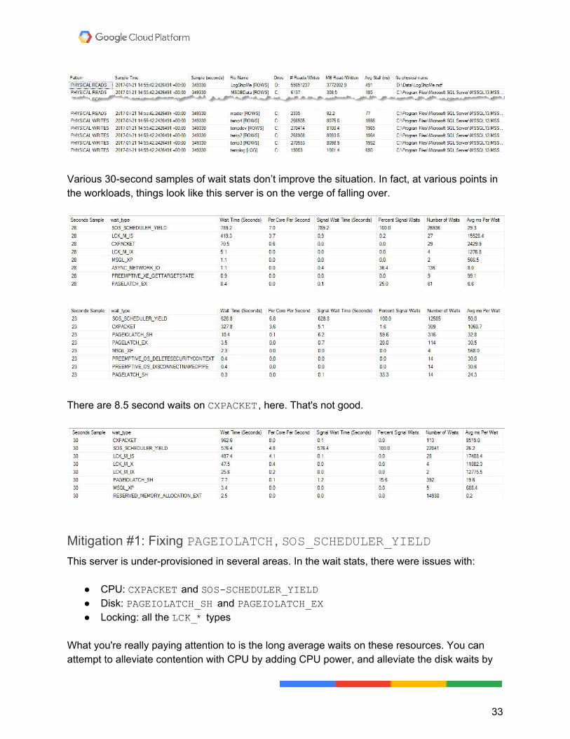
Various 30-second samples of wait stats don’t improve the situation. In fact, at various points in the workloads, things look like this server is on the verge of falling over.

There are 8.5 second waits on CXPACKET , here. That's not good.

Mitigation #1: Fixing PAGEIOLATCH , SOS_SCHEDULER_YIELD This server is under-provisioned in several areas. In the wait stats, there were issues with:

● CPU: CXPACKET and SOS-SCHEDULER_YIELD ● Disk: PAGEIOLATCH_SH and PAGEIOLATCH_EX ● Locking: all the LCK_* types

What you're really paying attention to is the long average waits on these resources. You can attempt to alleviate contention with CPU by adding CPU power, and alleviate the disk waits by

33

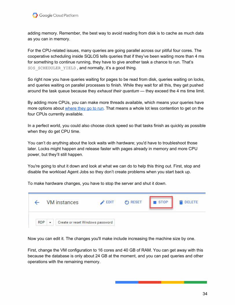
adding memory. Remember, the best way to avoid reading from disk is to cache as much data as you can in memory. For the CPU-related issues, many queries are going parallel across our pitiful four cores. The cooperative scheduling inside SQLOS tells queries that if they’ve been waiting more than 4 ms for something to continue running, they have to give another task a chance to run. That’s SOS_SCHEDULER_YIELD , and normally, it’s a good thing. So right now you have queries waiting for pages to be read from disk, queries waiting on locks, and queries waiting on parallel processes to finish. While they wait for all this, they get pushed around the task queue because they exhaust their quantum — they exceed the 4 ms time limit. By adding more CPUs, you can make more threads available, which means your queries have more options about where they go to run. That means a whole lot less contention to get on the four CPUs currently available. In a perfect world, you could also choose clock speed so that tasks finish as quickly as possible when they do get CPU time. You can’t do anything about the lock waits with hardware; you'd have to troubleshoot those later. Locks might happen and release faster with pages already in memory and more CPU power, but they’ll still happen. You're going to shut it down and look at what we can do to help this thing out. First, stop and disable the workload Agent Jobs so they don’t create problems when you start back up. To make hardware changes, you have to stop the server and shut it down.

Now you can edit it. The changes you'll make include increasing the machine size by one. First, change the VM configuration to 16 cores and 40 GB of RAM. You can get away with this because the database is only about 24 GB at the moment, and you can pad queries and other operations with the remaining memory.

34

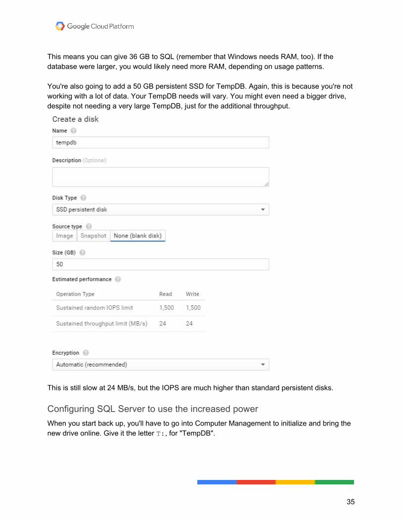
This means you can give 36 GB to SQL (remember that Windows needs RAM, too). If the database were larger, you would likely need more RAM, depending on usage patterns. You're also going to add a 50 GB persistent SSD for TempDB. Again, this is because you're not working with a lot of data. Your TempDB needs will vary. You might even need a bigger drive, despite not needing a very large TempDB, just for the additional throughput.

This is still slow at 24 MB/s, but the IOPS are much higher than standard persistent disks.

Configuring SQL Server to use the increased power When you start back up, you'll have to go into Computer Management to initialize and bring the new drive online. Give it the letter T: , for "TempDB".

35

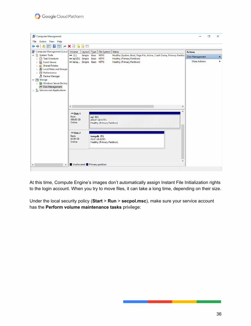
At this time, Compute Engine’s images don’t automatically assign Instant File Initialization rights to the login account. When you try to move files, it can take a long time, depending on their size. Under the local security policy (Start > Run > secpol.msc), make sure your service account has the Perform volume maintenance tasks privilege:

36

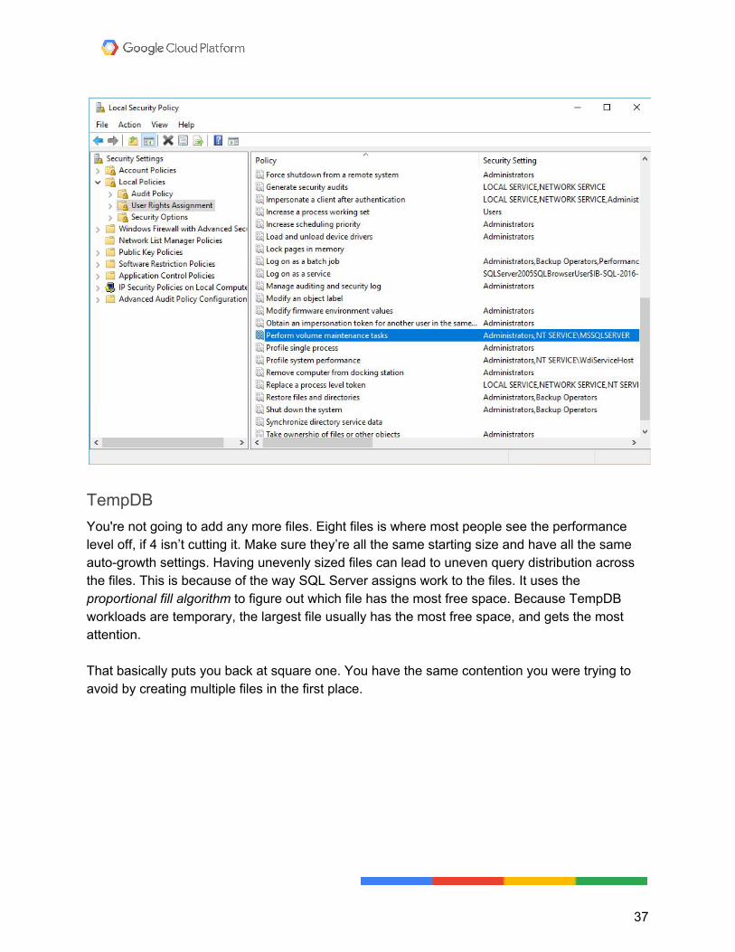
TempDB You're not going to add any more files. Eight files is where most people see the performance level off, if 4 isn’t cutting it. Make sure they’re all the same starting size and have all the same auto-growth settings. Having unevenly sized files can lead to uneven query distribution across the files. This is because of the way SQL Server assigns work to the files. It uses the proportional fill algorithm to figure out which file has the most free space. Because TempDB workloads are temporary, the largest file usually has the most free space, and gets the most attention. That basically puts you back at square one. You have the same contention you were trying to avoid by creating multiple files in the first place.

37

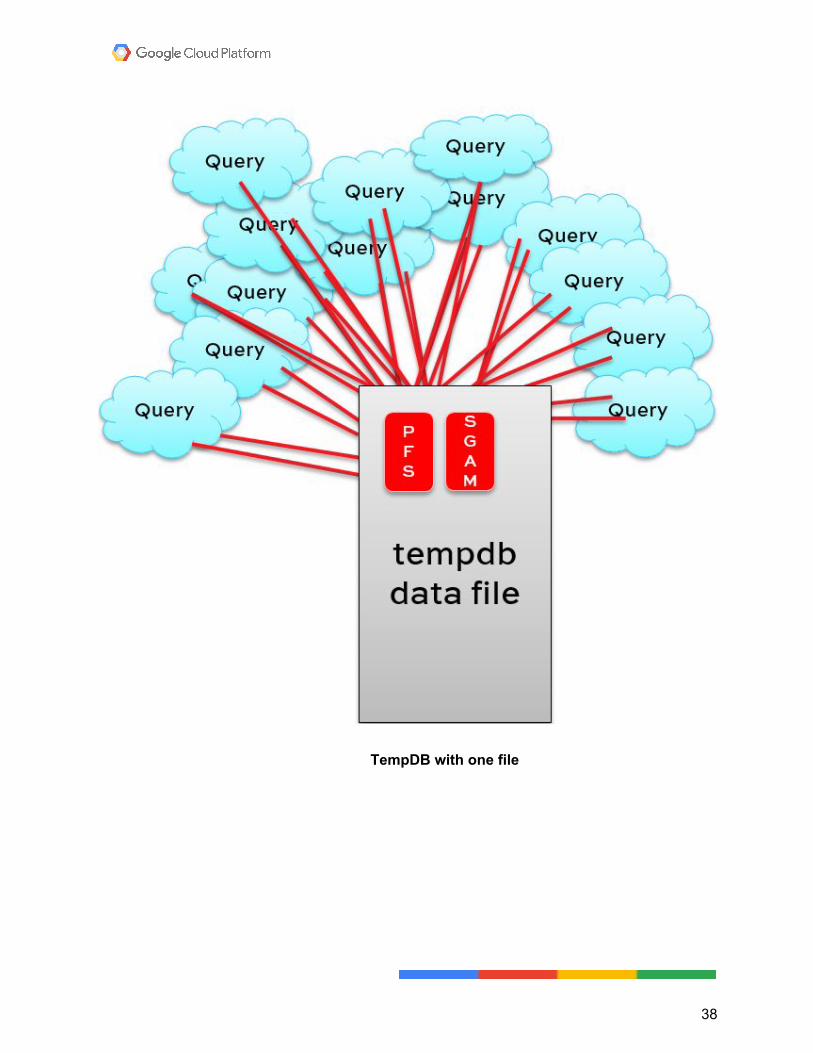
TempDB with one file

38

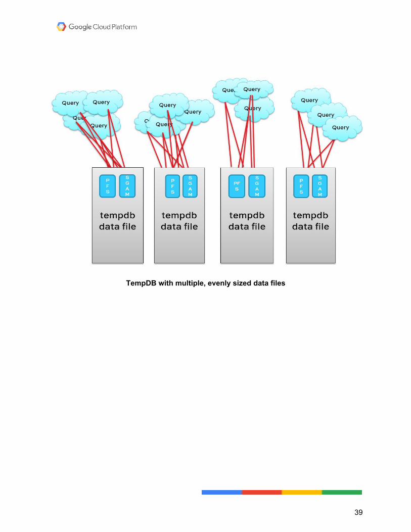
TempDB with multiple, evenly sized data files

39

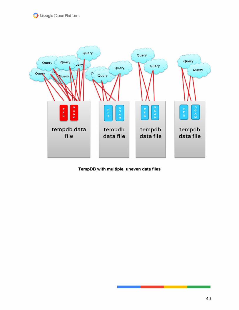
TempDB with multiple, uneven data files

40

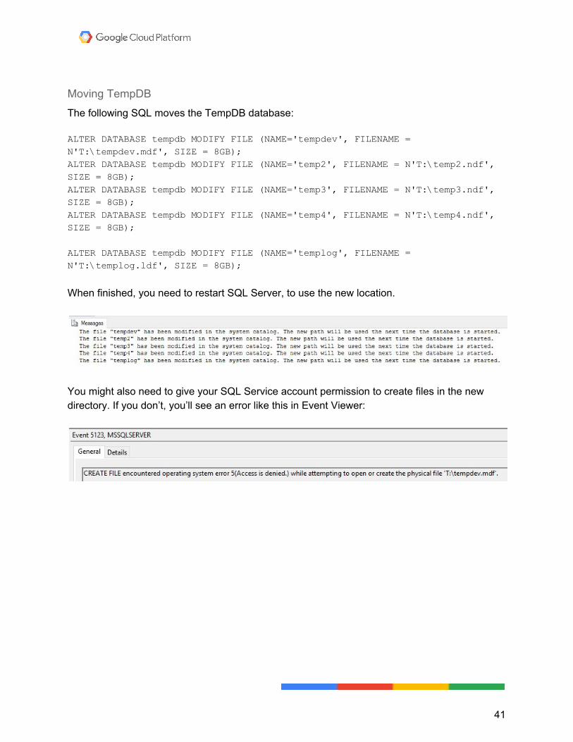
Moving TempDB The following SQL moves the TempDB database: ALTER DATABASE tempdb MODIFY FILE (NAME='tempdev', FILENAME = N'T:\tempdev.mdf', SIZE = 8GB); ALTER DATABASE tempdb MODIFY FILE (NAME='temp2', FILENAME = N'T:\temp2.ndf', SIZE = 8GB); ALTER DATABASE tempdb MODIFY FILE (NAME='temp3', FILENAME = N'T:\temp3.ndf', SIZE = 8GB); ALTER DATABASE tempdb MODIFY FILE (NAME='temp4', FILENAME = N'T:\temp4.ndf', SIZE = 8GB); ALTER DATABASE tempdb MODIFY FILE (NAME='templog', FILENAME = N'T:\templog.ldf', SIZE = 8GB);

When finished, you need to restart SQL Server, to use the new location.

You might also need to give your SQL Service account permission to create files in the new directory. If you don’t, you’ll see an error like this in Event Viewer:

41

Max server memory You’ll want to adjust Max Server Memory to a size appropriate to how much memory your server has. In this case, you have now have an 8 core, 40 GB RAM server, so set it to 36 GB (36 * 1024). Remember that this setting is in MB.

CPU You're going to leave MAXDOP and Cost Threshold for Parallelism alone here. This is to allow for greater concurrency. More queries can run across your new cores simultaneously if they’re using only four cores. You still want the same queries to go parallel — raising CTFP to a higher number would just force some queries to potentially run single threaded, but you really want them to stay parallel. That doesn’t help to increase performance. In fact it can do more harm than good.

Baseline #2: PAGEIOLATCH gone, SOS_SCHEDULER_YIELD still here After re-running the example workload for a bit, you can see how things are stacking up. You didn’t change any queries or indexes, you doubled CPU and RAM, and isolated TempDB on the SSD. You made these changes based on evidence you collected, not wild guesses. Increasing RAM serves two purposes. You fit all your data into memory, plus some extra to manage other caches. It also gives your queries and TempDB extra workspace to avoid spilling out to disk. Likewise, isolating TempDB to its own SSD gives you the fastest possible spills, if they do happen. Increasing CPU count helps you keep the workload spread over a larger number of cores, and hopefully reduces CPU contention. No changes you made will help the locking problems. While troubleshooting those is also outside the scope of this whitepaper, you can later enable a setting in SQL Server called Read Committed Snapshot Isolation (RCSI) to examine any impact on CPU and TempDB, and to remove reader/writer blocking from the wait stats noise.

42

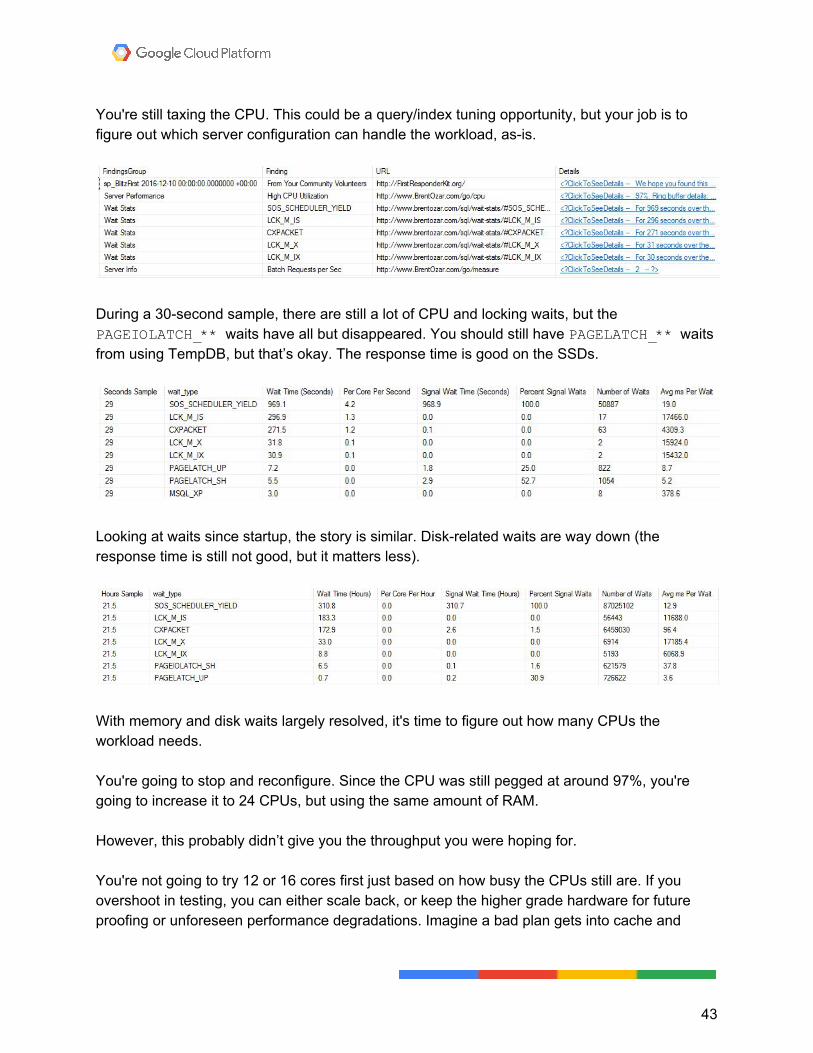
You're still taxing the CPU. This could be a query/index tuning opportunity, but your job is to figure out which server configuration can handle the workload, as-is.

During a 30-second sample, there are still a lot of CPU and locking waits, but the PAGEIOLATCH_** waits have all but disappeared. You should still have PAGELATCH_** waits from using TempDB, but that’s okay. The response time is good on the SSDs.

Looking at waits since startup, the story is similar. Disk-related waits are way down (the response time is still not good, but it matters less).

With memory and disk waits largely resolved, it's time to figure out how many CPUs the workload needs. You're going to stop and reconfigure. Since the CPU was still pegged at around 97%, you're going to increase it to 24 CPUs, but using the same amount of RAM. However, this probably didn’t give you the throughput you were hoping for. You're not going to try 12 or 16 cores first just based on how busy the CPUs still are. If you overshoot in testing, you can either scale back, or keep the higher grade hardware for future proofing or unforeseen performance degradations. Imagine a bad plan gets into cache and

43

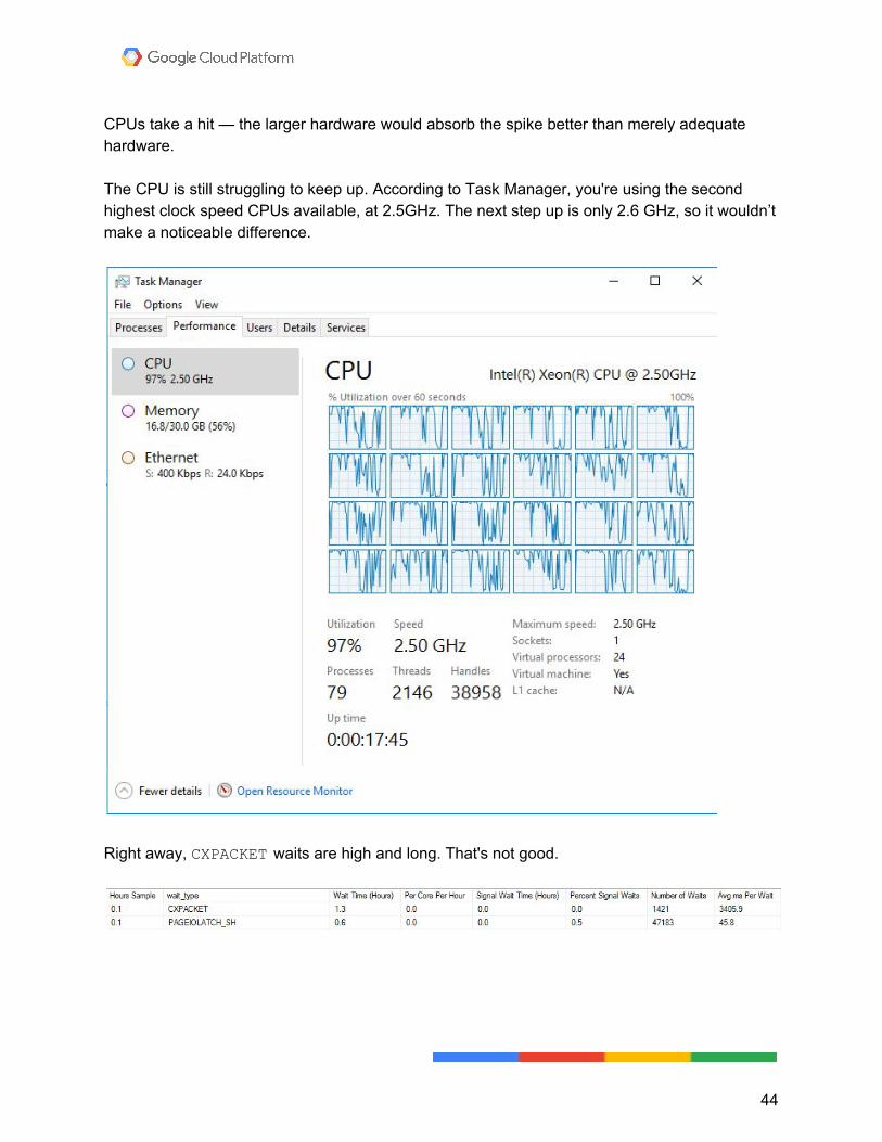
CPUs take a hit — the larger hardware would absorb the spike better than merely adequate hardware. The CPU is still struggling to keep up. According to Task Manager, you're using the second highest clock speed CPUs available, at 2.5GHz. The next step up is only 2.6 GHz, so it wouldn’t make a noticeable difference.

Right away, CXPACKET waits are high and long. That's not good.

44

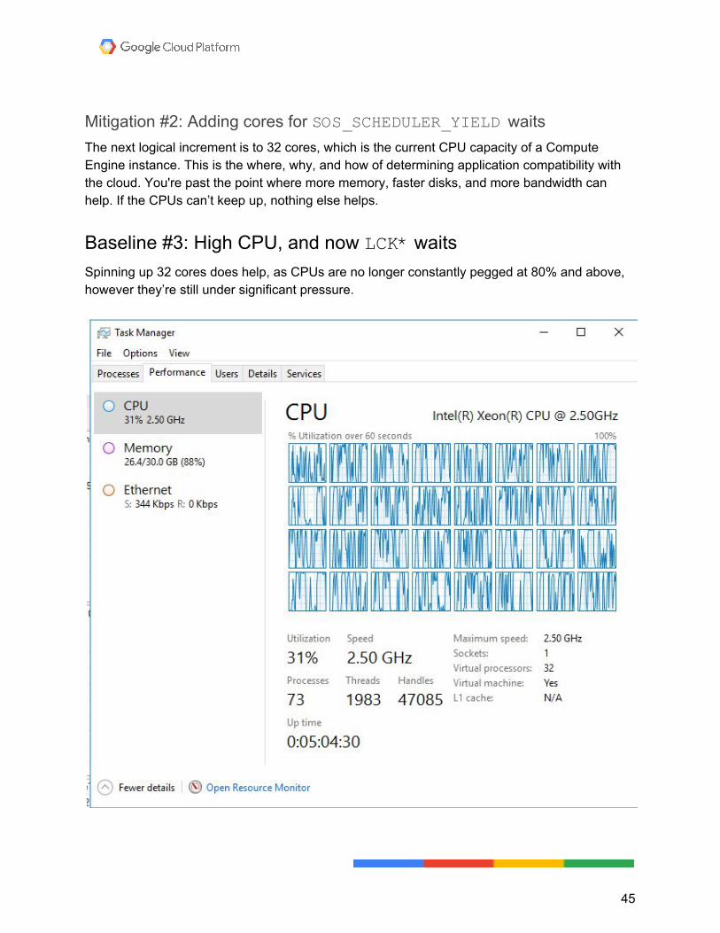
Mitigation #2: Adding cores for SOS_SCHEDULER_YIELD waits The next logical increment is to 32 cores, which is the current CPU capacity of a Compute Engine instance. This is the where, why, and how of determining application compatibility with the cloud. You're past the point where more memory, faster disks, and more bandwidth can help. If the CPUs can’t keep up, nothing else helps.

Baseline #3: High CPU, and now LCK* waits Spinning up 32 cores does help, as CPUs are no longer constantly pegged at 80% and above, however they’re still under significant pressure.

45

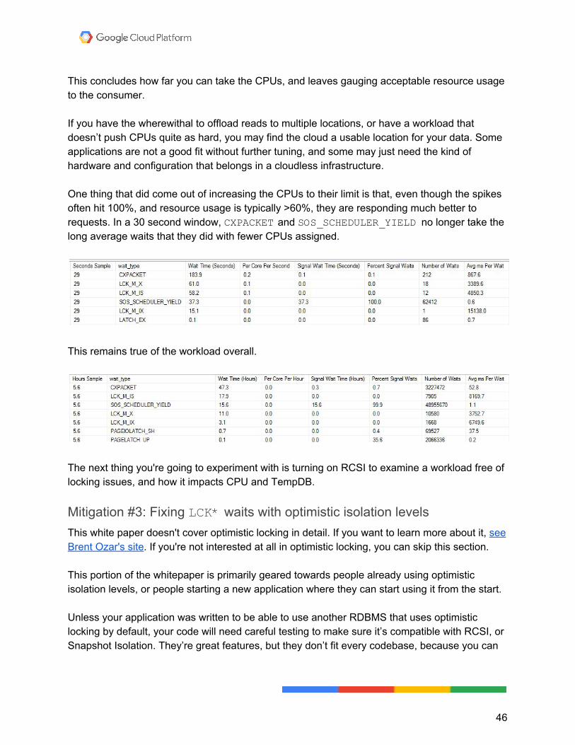
This concludes how far you can take the CPUs, and leaves gauging acceptable resource usage to the consumer. If you have the wherewithal to offload reads to multiple locations, or have a workload that doesn’t push CPUs quite as hard, you may find the cloud a usable location for your data. Some applications are not a good fit without further tuning, and some may just need the kind of hardware and configuration that belongs in a cloudless infrastructure. One thing that did come out of increasing the CPUs to their limit is that, even though the spikes often hit 100%, and resource usage is typically >60%, they are responding much better to requests. In a 30 second window, CXPACKET and SOS_SCHEDULER_YIELD no longer take the long average waits that they did with fewer CPUs assigned.

This remains true of the workload overall.

The next thing you're going to experiment with is turning on RCSI to examine a workload free of locking issues, and how it impacts CPU and TempDB.

Mitigation #3: Fixing LCK* waits with optimistic isolation levels This white paper doesn't cover optimistic locking in detail. If you want to learn more about it, see Brent Ozar's site. If you're not interested at all in optimistic locking, you can skip this section. This portion of the whitepaper is primarily geared towards people already using optimistic isolation levels, or people starting a new application where they can start using it from the start. Unless your application was written to be able to use another RDBMS that uses optimistic locking by default, your code will need careful testing to make sure it’s compatible with RCSI, or Snapshot Isolation. They’re great features, but they don’t fit every codebase, because you can

46

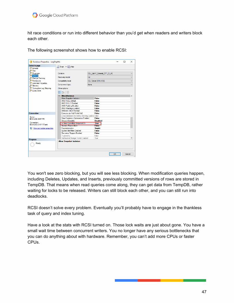
hit race conditions or run into different behavior than you’d get when readers and writers block each other. The following screenshot shows how to enable RCSI:

You won't see zero blocking, but you will see less blocking. When modification queries happen, including Deletes, Updates, and Inserts, previously committed versions of rows are stored in TempDB. That means when read queries come along, they can get data from TempDB, rather waiting for locks to be released. Writers can still block each other, and you can still run into deadlocks. RCSI doesn’t solve every problem. Eventually you’ll probably have to engage in the thankless task of query and index tuning. Have a look at the stats with RCSI turned on. Those lock waits are just about gone. You have a small wait time between concurrent writers. You no longer have any serious bottlenecks that you can do anything about with hardware. Remember, you can’t add more CPUs or faster CPUs.

47

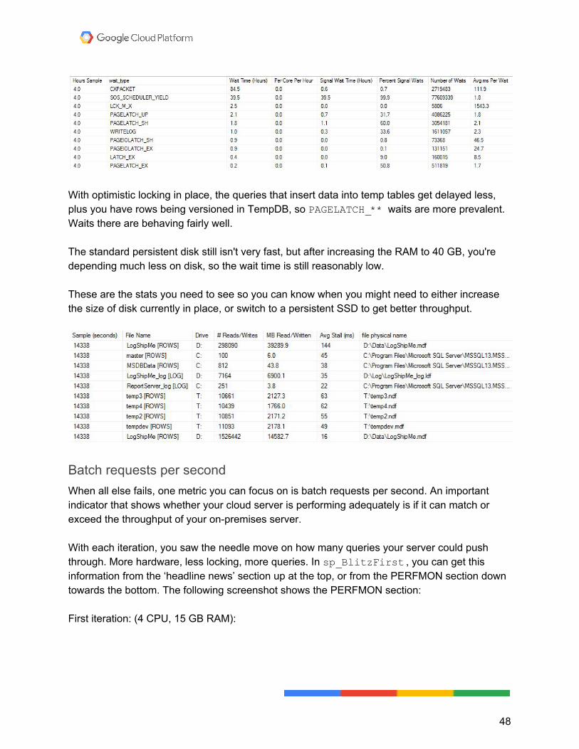
With optimistic locking in place, the queries that insert data into temp tables get delayed less, plus you have rows being versioned in TempDB, so PAGELATCH_** waits are more prevalent. Waits there are behaving fairly well. The standard persistent disk still isn't very fast, but after increasing the RAM to 40 GB, you're depending much less on disk, so the wait time is still reasonably low. These are the stats you need to see so you can know when you might need to either increase the size of disk currently in place, or switch to a persistent SSD to get better throughput.

Batch requests per second When all else fails, one metric you can focus on is batch requests per second. An important indicator that shows whether your cloud server is performing adequately is if it can match or exceed the throughput of your on-premises server. With each iteration, you saw the needle move on how many queries your server could push through. More hardware, less locking, more queries. In sp_BlitzFirst , you can get this information from the ‘headline news’ section up at the top, or from the PERFMON section down towards the bottom. The following screenshot shows the PERFMON section: First iteration: (4 CPU, 15 GB RAM):

48

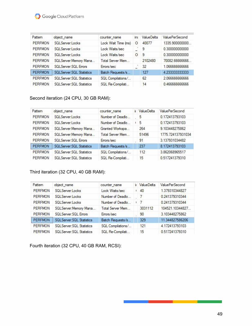
Second iteration (24 CPU, 30 GB RAM):

Third iteration (32 CPU, 40 GB RAM):

Fourth iteration (32 CPU, 40 GB RAM, RCSI):

49

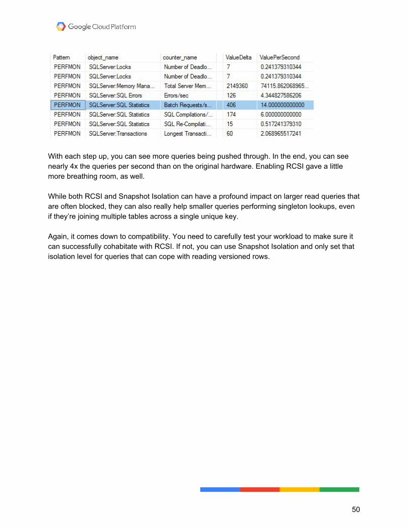
With each step up, you can see more queries being pushed through. In the end, you can see nearly 4x the queries per second than on the original hardware. Enabling RCSI gave a little more breathing room, as well. While both RCSI and Snapshot Isolation can have a profound impact on larger read queries that are often blocked, they can also really help smaller queries performing singleton lookups, even if they’re joining multiple tables across a single unique key. Again, it comes down to compatibility. You need to carefully test your workload to make sure it can successfully cohabitate with RCSI. If not, you can use Snapshot Isolation and only set that isolation level for queries that can cope with reading versioned rows.

50