NASA CONTRACTOR REPORT

NASA C R - 1 8 3 5 2 8

HOT W I R E ANEMOMETER MEASUREMENTS I N THE UNHEATED A I R FLOW TESTS OF THE SRB NOZZLE-TO- raSE J O I N T

By N. Ramachandran Universities Space Research Association 4950 Corporate Drive, Suite 100 Huntsville, Alabama 35806

(hASA-Cb-183528) tlOT L I R E AbEGCEETEB N89- 176 19 C E A S U R E H E N T S IN 'LEE UIEfATEC L l E i ELCW lBSBS C € 161: S E E NCZZIE-TG-C&SE JCIb'I Einal Rep6rt ( C n i v e r s i ties Srace B €sea rcb. dEr oci a t i o n ) Unclat 44 1; CSCL 218 63/20 0385618

Final Report

December 1988

n

Prepared for NASA-Marshall Space Flight Center Marshall Space Flight Center, Alabama 35812

https://ntrs.nasa.gov/search.jsp?R=19890008248 2018-07-01T20:50:14+00:00Z

ACKNOWLEDGMENTS

The author wishes MSFC, for his continued anemometer measurement

to extend his sincere gratitude to M r . John Heaman, NASA/ zeal and encouragement in the development of the hot-wire capability at MSFC. The discussions-the author had with him

I were very useful in charting this developmental process and using it in tests of flight * hardware. The author wishes to express his appreciation to M r . Dave Bacchus, the technical monitor, M r . Jack Hengel, the project engineer, and M r . Hal Gwin for their help and guidance during the course of the project. A special thanks is extended to M r . James McAnally and M r . Leroy H a i r for their help and input during the hot-wire measurement phase of the project.

The author wishes to extend thanks to Messrs. Teddy Stephens, Willard Edwards, Carl Walker, and Dickie Mitchell for their help in the operations of the wind tunnel and the experimental facility. The help of co-op students Andrew Smith, Mark Powell, and Steve Gaddis is also appreciated.

.

TABLE OF CONTENTS

Page .

1 1 . 0 INTRODUCTION .......................................................... 2 . 0 TEST FACILITY AND MODEL DESCRIPTION .............................. 2

2 . 1 Test Facility ........................................................ 2 . 2 Model Description .................................................... 2

2

3 3 . 0 HOT WIRE ANEMOMETRY ................................................. 3 . 1 MSFC Hot-wire Anemometer Hardware ................................ 3.2 Hot-wire Anemometer Calibration ..................................... 3 . 3 Data Reduction ......................................................

3 3 4

3 . 3 . 1 Temperature Correction ...................................... 3 . 3 . 2 Correction for Probe Orientation .............................. 3 . 3 . 3 Correction for Static Pressure ................................

4 5 5

4.0 PRELIMINARY TESTS ..................................................... 6

4 . 1 Probe Positioning and Orientation .................................... 6

5 . 0 RESULTS AND DISCUSSION .............................................. 7

5 . 1 Vented- Joint Configuration .......................................... 5 . 2 Type 1 Bonded Joint (Debonds 2 and 4) ............................. 5 . 3 Type 2 Bonded Joint (Debonds 5. 6. and 8) .........................

7 8 9

5 . 3 . 1 Debond 5 ..................................................... 5 . 3 . 2 Entrance Region Flow Characterization ....................... 5 . 3 . 3 Debonds 6 and 8 .............................................

10 10 11

12 6.0 CONCLUSIONS ........................................................... REFERENCES .................................................................. 13

iii

LIST OF ILLUSTRATIONS

Figure Title Page

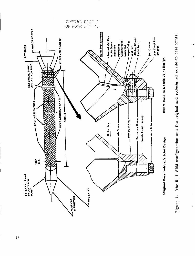
The 51-L SRM configuration and the original and redesigned nozzle-to-case joints .................................................. 16

2. The 2-D SRB nozzle-to-case joint model ............................... 17

1. -

3 . Debond configurations for the SRB joint tests ........................ 18

4. 19 Probe orientation and schematic of the TSI calibrator ................. 5 . Hot wire calibration using the TSI calibrator .......................... 20

6 . Bore velocity distribution during the HWA calibrations ................ 20

7. Hot wire anemometer calibration, Po = 60 lb/in. ...................... 8. Hot wire anemometer calibration, Po = 60 lb/in. ...................... 9. Hot wire anemometer calibration, Po = 60 lb/in. ......................

10. Machined plug for holding the hot wires .............................. 22

I I I

21

21

22

2

2

I 2

11. Geometry of the gap between the O-rings ............................. 23

12. Effect of gap width; velocity data in the vented joint, liner 1 ........ 24

13. Effect of gap width; velocity data in the vented joint, liner 4 ... .... 24

~ 14. Normalized O-ring gap velocity distribution ; vented joint ............. 25

15.

16.

17.

Normalized O-ring gap velocity distribution; Debond 2 bonded joint ... 25

26

27

O-ring gap velocity distribution; Debond 4 bonded joint .............. Normalized O-ring gap velocity distribution; Debond 4 bonded joint ...

I 28 18.

19. 29

Type-2 debond models; model geometry and flow field.. ............... Effect of gap width on the gap velocities; Type-2 bonded joint .......

20. 29

21. 30

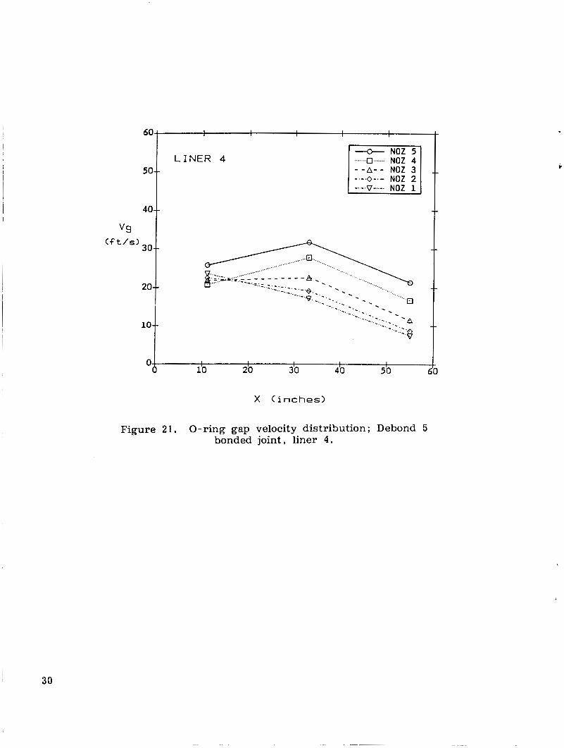
22. Heat transfer coefficient distribution; Debond 5 bonded joint.. ........ 31

O-ring gap velocity distribution; Debond 5 bonded joint . liner 1 . . .... O-ring gap velocity distribution; Debond 5 bonded joint, liner 4 . . ....

I 23. Normalized O-ring gap velocity distribution; Debond 5 bonded joint ... 32

24. Effect of probe orientation on the gap velocities; Debond 8 I bonded joint .......................................................... 33

iv

a

LIST OF ILLUSTRATIONS (Concluded)

Figure Title Page

25. O-ring gap velocity distribution; Debond 6 bonded joint ............. 34

26. Normalized O-ring gap velocity distribution, Debond 6 bonded joint ......................................................... 35

27. O-ring gap velocity distribLition; De'bond 8 bonded joint ............. 36

28. Normalized O-ring gap velocity distributio.,; Debond 8 bonded joint ......................................................... 37

.

V

LIST OF TABLES

Table Title

1 . 2 . Bore Velocity and Pressure Data ..................................... 3 . Gap Dimensions .......................................................

Dimensions of Auxiliary Items ......................................... Page

14

15

23

.

CONTRACTOR REPORT

HOT WIRE ANEMOMETER MEASUREMENTS IN THE UNHEATED AIR FLOW TESTS OF THE SRB NOZZLE-TO-CASE JOINT

1.0 INTRODUCTION

After the 51-L mission of the Space Shuttle, considerable attention was focused on the development of redesigns for the Solid Rocket Motor (SRM) case-to-field joints and the nozzle-to-case joint. joint robustness capable of better withstanding the dynamic pressure loads during SRM burns. problems were noticed during previous shuttle flights and these were sought to be remedied in the redesign effort. The 51-L SRM configuration is shown in Figure 1 along with insets showing the original and redesigned nozzle-to-case joints. In the original design, the high ignition pressures of the SRM caused a radial expansion of the motor case leading to a widening of the joint with subsequent O-ring erosion due to their improper sealing action. been added in the redesign to minimize the joint sealing-gap opening. has also been added in the joint to serve as a hot gas seal and prevent the adhesive or hot propellant gases from reaching the primary O-ring vicinity. insulation has been modified to be sealed with polysulfide adhesive.

The new designs called for added safety features and

The nozzle-to-case joint has had several instances where O-ring erosion

Additional radial bolts with "Stato-0-seals" have A wiper O-ring

Also, the internal

This particular report deals w i t h the Hot Wire Anemonieter (HWA) measurements made in the Solid Rocket Booster (SRB) nozzle-to-case joint cold flow tests and repre- sents an exploratory effort at NASA/MSFC in the use of hot wire/film anemometers in hardware testing and evaluation. These cold flow tests were planned and undertaken in an effort to glean additional information and data on the circumferential flow induced in the SRB joints due to pressure g'radients imposed as a result of nozzle gimbal and/or unsymmetrical propellant burn. approximately 120 deg of the SRB joint arc during SRB burn. linear model of the actual circular SRB joint w i t h imposed axial pressure gradients used to simulate the circumferential flow behavior in the SRB. The hot wire tests were intended to supplement the pressure and heat transfer measurements characteriz- ing the flow and thermal fields in the redesigned joint of the SRB and provide velocity data in the s m a l l gap regions between the O-rings where conventional Pitot-static probes cannot be used. tioned earlier, calls for an adhesive sealant in place of the putty used prior to the 51-L mission, in the insulation gap that arises during the stacking process of the SRB. The sealant is expected to prevent hot propellant gases from reaching the O-rings in the joint and, hence, preclude any significant erosion problems. The present series of tests seek to evaluate the design by testing the effect of adhesive flaws (debonds) in the redesigned joint. Additional information regarding other tests concerning this phenomenon and geometry can be obtained from References 1 and 2.

This circumferential flow is estimated to exist in The test hardware is a

The new design of the SRB nozzle-to-case joint, as men-

#

The test series for the HWA is comprised of blow-down runs of unheated air flow through the 2-D model with different cross-sectional changes representing different joint configurations. the test matrix reflecting parametric changes of the model M e t Mach number, the imposed axial pressure gradient, and the joint gaps.

A generic vented joint and six debond joints were tested, with

Objectives :

The HWA tests were undertaken with the following specific objectives in mind:

1. Develop in-house capability for the calibration and use of hot wire/film anemometers.

2. Develop software for the HWA output corrections for use in an environment . different from calibration conditions. might be temperature stratified or where static pressure changes might be encountered. Wall correction effects are also possibilities that should be taken into account.

This helps the use of the HWA in flows which

. 3. Make HWA measurements in the SRB nozzle joint tests. This objective

involved preliminary tests where HWA data could be corroborated by velocity measure- ments by other independent means and then subsequent stand-alone HWA measurements.

I 2 .0 TEST FACILITY AND MODEL DESCRIPTION

2 . 1 Test Facility

The hot wire tests were done in the SRM leg of the Engine A i r Flow Facility 2 (EAFF) in the blow-down mode. Pressurized air at a total pressure (Po = 60 lb/in. )

is fed from the main supply tank through a 16-in. diameter pipe to the 2-D nozzle-to- case joint model. This pressure rate translates to a mass flow rate of about 3 lbs/sec for the highest model Mach number of 0.15. The supply pressure decreases by about 0.1 psi/sec of operation during the tests. Thus, during a typical run time for a test of about 30 sec, the total pressure drop is about 3 psi. Additional details about the test facility and its capabilities are documented in Reference 1.

2 . 2 Model Description

The general arrangement of the 2-D model is shown in Figure 2. Both the generic vented joint and the nozzle-to-case joint with debonds utilized this basic setup. The model itself is 65-in. long with a bore entrance diameter of 3.124 in. A s illustrated in the inset, the bore connects to the O-ring location by means of a slot whose dimensions can be varied. Bonding material placed in this slot region simulates the bonded joint with built-in flaws that model the different burn throughs or debonds that were tested. 2-D joint hardware without any bonding material. The debond configurations were basically in two major groups, Type 1 and Type 2. Type 1 debond models represent the full-length, partial-width concept with 65-in. long shims used to vary the gap width between the model bore and the wiper O-ring location. Thus, these configura- tions are similar to the vented joint case with restrictions placed on the slot width. The Type 2 debonds are of the full-width , partial-length configuration representative of flaws in the insulation bonding material. These simulated blow holes allow the flow of air through restricted channels in the model inlet and exit regions only, with the region in-between being completely blocked off. Rubber gaskets were used to sirnu- late the different debond geometries. the model bore (representing the circumferential flow region) and the wiper O-ring location is sealed off except for the regions of modeled flaws. dimensions associated with different debond configurations (Ids) are detailed in Figure 3.

The generic vented joint was modeled using the same

Thus, in the Type 2 debonds, the gap between

The different slot

2

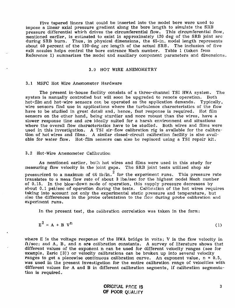
Five tapered liners that could be inserted into the model bore were used to impose a linear axial pressure gradient along the bore length to simulate the SRB pressure differential whirh drives the circumferential flow. This circumferential flow, mentioned earlier, is estimated to exist in approximately 120 deg of the SRB joint arc during SRB burn. Thus, in physical dimensions, the 65-in. model length represents about 60 percent of the 120-deg arc length of the actual SRB. The inclusion of five exit nozzles helps control the bore entrance Mach number. Reference 1) summarizes the model and auxiliary component parameters and dimensions

Table 1 (taken from

3 . 0 HOT WIRE ANEMOMETRY

3.1 MSFC Hot Wire Anemometer Hardware

The present in-house facility consists of a three-channel TSI HWA system. The system is manually controlled but will soon be upgraded to remote operation. Both hot-film and hot-wire sensors can be operated as the application demands. Typically, wire sensors find use in applications where the turbulence characteristics of the flow have to be studied in great detail and, hence, fast response is required. Hot f i lm sensors on the other hand, being sturdier and more robust than the wires, have a slower response time and are ideally suited for a harsh environment and situations where the overall flow characteristics have to be studied. Both wires and films were used in this investigation. A TSI air-flow calibration rig is available for the calibra- tion of hot wires and films. A similar closed-circuit calibration facility is also avail- able for water flow, Hot-film sensors can also be replaced using a TSI repair kit.

3.2 Hot -Wire Anemometer Calibration

A s mentioned earlier, both hot wires and f i l m s were used in this study for measuring flow velocity in the joint gaps. pressurized to a maximum of 60 lb/in. translates to a mass flow rate of about 3 lbs/sec for the highest model Mach number of 0.15. ahout 0 .1 psi/sec of operation during the tests. taking into account not only the experimental static pressure and temperature, but also the differences in the probe orientation to the flow during probe calibration and experiment runs,

The SRB joint tests utilized shop air for the experiment runs. This pressure rate

In the blow-down mode of operation, this supply pressure decreases by Calibration of the hot wires requires

In the present test the calibration correlation was taken in the form:

E 2 = A + B V n

where E is the voltage response of the HWA bridge in volts; V is the flow velocity in A/sec; and A , B, and n are calibration constants. A survey of literature shows that different values of the exponent n can be used for different velocity ranges (see for example, Zaric [ 3 ] ) or velocity calibrations can be broken up into several velocity ranges to get a piecewise continuous calibration curve. An exponent value, n = 0.5, was used in the present investigation for the entire calibration range of velocities with different values for A and B in different calibration segments, if calibration segmenta- tion is required.

ORllGlNAL PACE is OF BOOR QUAtiTY

3

For velocity calibration at ambient conditions, a TSI 1125 probe calibrator is available in which the probe can be positioned in either the end or cross flow orienta- tion, as the application demands. Additional information about the calibrator can be obtained from Reference 4. Figure 4 shows the possible probe orientations along with a schematic of the calibrator. A typical calibration curve is shown in Figure 5 with the resultant least-squares fit giving a calibration of the form:

E ~ = A + B V 0.5

This calibration is valid under the same conditions of static pressure and tem- perature as those present during the calibration process. Thus, for any changes in the pressure and temperature conditions, corrections have to be applied to the HWA output to deduce the correct flow velocity. that the hot wires would be calibrated at the operating pressure level of 60 lb/in.2 itself in the model bore, and this approach would require only temperature correc- tions during the data reduction stage.

I In the present study, it w a s decided

3 . 3 Data Reduction

The methodology adopted for HWA data reduction is outlined in this section. The terminology used here refers to the experiment conditions by the suffix e and the calibration conditions by the suffix c. Using this nomenclature, the calibration equation (2) can be recast into the following form

= (A + B V o a 5 ) (T - EC S Te) ( 3 )

where Ts is the probe operating temperature (about 482OF in this case) and the other variables in the equation are as defined earlier. It is to be noted that the calibration given by equation ( 3 ) is valid only for the calibration conditions, Pc (14.7 psia) and the calibration temperature Tc , respectively. from the calibration conditions, corrections have to be applied for the probe orienta- tion and the static pressure and temperature differences. in the data reduction sequence to get the correct flow velocity.

For experimental conditions different

These steps are incorporated

3 . 3 . 1 Temperature Correction

The response of the HWA during an experimental run can be written in the following form [from equation ( 3 ) ] :

Te)

From equations ( 3 ) and ( 4 ) , one gets

4

OF POOR QWWTY

which can be used to get the temperature-corrected hot-wire response.

3.3.2 Correction for Probe Orientation

It is to be noted that if the probe is calibrated in end flow and used during experiments in cross flow (Fig. 41, a higher velocity (higher than the actual) is pre- dicted by the calibration equation ( 2 ) . have to be applied to deduce the correct flow velocity. probe was calibrated and used in cross flow, thus obviating the probe orientation corrections.

Hence, corrections using pitch factor charts In the present study, the

3.2.3 Correction for Static Pressure

The HWA is sensitive to the mass flow rate pV, where p is the fluid density, rather than the flow velocity V, itself. the calibration conditions requires a pressure correction. behavior, the following equation can be written :

Thus, a change in the static pressure from Assuming ideal gas

vc Pc = ve Pe

and thus

Since in this investigation the calibrations were done in the model bore under the operating pressure conditions (60 lb/in. 2 > , no pressure corrections were required.

on either side of the HWA locatioii and a linear interpolation of the velocity data to arrive at the velocity at the HWA station itself. Figure 6 with the HWA positioned at location D (Fig. 2) in the model bore and velocity data a t other locations measured using Pitot-static probes. the final calibrations of three probes at 60 Ibs/in. and corresponding flow tempera- tures. the supply pressure was initially adjusted to 61 lbs/in.2 to account for the pressure drop during the blow down sequence, giving an average pressure level of 60 lbs/in. during an entire run. 60 lbs/in.2, then equation (7) was dsed to correct for the minor pressure differences.

A typical HWA calibration in the bore utilized Pitot-static velocity measurements

Such a calibration run is shown in

Figures 7 through 9 show

Since an experimental run took approximately 30 sec of the SRM leg operation, I

2 If during a run the mean pressure level was different from

5

4.0 PRELIMINARY TESTS

The MSFC SRB tests are discussed in the following sections. The hot-wire tests were done subsequent to the SRB heat-transfer tests that were used to determine the thermal response of the 2-D model using slug-type calorimeters. themselves positioned in the calorimeter locations using specially machined plugs similar in design to the calorimeters. Figure 10 shows the drawing of a typical plug used to hold the hot wires. linear (in-out) motion of the HWA in addition to rotational freedom used to adjust the orientation of the hot wires. The HWA data were first taken for the generic vented- joint configuration followed by tests for debond-joint models.

The hot wires were

The plugs made of aluminum were leak proof and afforded a

The HWA tests were conducted in two phases. In the Phase 1 of operations, the HWA calibration runs and preliminary tests were done to check the instrumentation setup and accuracy. The generic vented-joint tests were also completed during this phase. channels operational and, hence, the test sequence was conducted in two stages. In the first stage, hot wires were positioned at locations QAB3 and QBC3 (Fig. 2) and during the second stage at locations QCD3 and QEF3, respectively. The results from the two stages were combined for subsequent data analysis to get the axial velocity distribution in the gap.

In this test phase, the TSI system used for the HWA tests had only two

In Phase 2, the TSI system was upgraded to three-channel capability and the tests in the different debond models were undertaken. Both Type 1 and Type 2 debond models were tested, and additional runs were made to try to characterize the entrance region flow field in some of the configurations.

4 . 1 Probe Positioning and Orientation

The cross section of the 2-D test hardware, showing additional details of the gap The terminology used to designate the gaps between geometry, is shown in Figure 11.

the wiper and closure O-rings is also provided in Table 3. Gaps 2 and 3 were always changed simultaneously and maintained the same. Gap 1, however, was independently changed. During the preliminary HWA tests, Gap 1 (between the O-rings) was main- tained fixed at 0.01 in. and Gaps 2 and 3 were kept at either 0.05 in. or 0.042 in. Owing to the small gap sizes, all HWA measurements were made with the probes posi- tioned in the center of the gap. Also, the measurements were made with the probes positioned in cross flow, the same orientation as that used during the probe calibra- tions. Thus, no probe orientation corrections had to be made to the HWA outputs. Comparison of the HWA zero readings (with no flow) in the gap and those recorded during calibrations showed no wall proximity effects. in the output were the variations due to the change in the ambient temperature. Thus, no wall corrections had to be made to the HWA readings. The HWA signals were checked for the probe angular orientation as was done during the calibration runs in the model bore. Probe rotation by 5 deg, in either a clockwise or a counter- clockwise direction, Lid not show any appreciable change in the readings as discerned from manual (visual) data sampling. flow to be essentially parallel to the gap length for different joint configurations. Based on these observations, it was decided to position the probe in cross flow in the normal orientation (90 deg to the flow). help of gauge blocks, and normal probe orientation was obtained using a circular dial with angle calibration.

The only minor changes noted

I

Prior oil flow tests in the model had shown the

Gap center positioning was done with the

6

The accuracy and repeatability of the HWA measurements were assessed by measuring the bore velocity with different liners in the model and comparing the data to those obtained in earlier tests using Pitot-static probes. in the HWA measurements was found in these tests. checked subsequelit to every joint change and repeated if a drift was noticed. the data was acquired manually in the initial phase, velocity data accuracy based on the highest and lowest readings of the HWA was found to be within 5 percent for high velocities ( > 20 f t /sec) and to within 8 percent for lower velocities ( < 20 ft /sec) . The flow was considerably turbulent but quantitative information of the turbulence level was not obtained in these tests.

Less than 2 percent error The HWA calibrations were

A s

5.0 RESULTS AND DISCUSSION

The HWA measurements in the vented joint and the Type 1 and Type 2 debond- joint models are presented in the following sections.

5.1 Vented- Joint Configuration

In these model tests the hot wires were placed at axial locations QAB3, QBC3, QCD3, and QEF3 at the gap center. two-channel hot-wire operation and liners 1 and 4 were used to impose the axial pres- sure gradient in the model bore. tribution for two different sizes of the gap between the O-rings. The abscissa is the axial distance from the model inlet section. general observations can be made :

The tests were carried out in two stages with a

Figures 1 2 and 13 show the gap velocity V dis- g '

From these two figures the following

a. Liner 1 (Fig. 12): The axial velocity profile is essentially uniform for the smaller nozzles. Some acceleration of the flow field in the joint gap is seen as the bore inIet Mach number is increased. ft/sec for an inIet Mach number of 0.10 with the smallest velocity around 20 ft/sec for a Mach number of 0.03.

The maximum velocity can be as high as 80

b. Liner 4 (Fig. 13): A s tabulated in Table 1, this liner is only 52.25-in. long and the hot-wire position QAB3 corresponds to a gap location where there is no liner in the model bore. relatively small magnitude with large attendant fluctuations than at other hot wire locations. The flow downstream of the location QAB3 is similar to that seen for liner 1 except for smaller velocities and higher turbulence levels. The velocity gradient is steeper for the smaller gap than for the larger gap configuration. age velocity (excluding location QAB3) for the larger gap is about 40 ft/sec as com- pared to 32 ft/sec for the smaller gap.

Thus, the flow corresponding to this hot-wire location shows a

The maximum aver-

c . nozzles. than those for the latter case.

The velocities are higher for the larger nozzles in comparison to the smaller This is because the larger nozzles correspond to a higher inlet Mach number

d , The flow for liner 1 ( w i t h small exit diameter) is higher in general than that for liner 4 (with larger exit diameter). into the gap region in the former case (greater axial pressure gradient) than in the latter case (smaller axial pressure gradient).

This trend is because more air is forced

7

e. A smaller dimension for Gap 2 drops the maximum velocity marginally (about 12 percent) for liner 1 and the same general flow characteristics as seen for the larger gap prevail in the smaller gap geometry. tion increases the maximum velocity by about 25 percent with similar trends for the different nozzles tested. An examination of the heat transfer data from runs con- ducted prior to the hot-wire tests revealed that the measured velocity changes for the two gap sizes would not transform into any significant changes in the heat transfer rate. Hence, all subsequent joint and debond model tests were made with the nominal O-ring gap widths typical of the actual flight hardware. This meant Gap 1 = 0.006 in. and Gaps 2 and 3 = 0.046 in.

For liner 4, however, the gap reduc-

Velocity data from Figures 12 and 13 are presented in Figure 14, normalized with the inlet bore velocity, Vb. Mach number, and the velocity in the bore at station A (Fig. 2) obtained from pitot- static measurements are listed in Table 2 for liners 1 and 4 that were used in this study. From the figure, typically higher velocities are seen for liner 1 than those for liner 4. The data shows the velocity buildup to reach about 75 percent and 30 percent of the bore inlet velocity for liners 1 and 4 , respectively, with the axial location of this maximum velocity corresponding to around 33 and 22 in . , respectively, for the two liner configurations.

The linear axial pressure gradient, the bore inlet

5.2 Type 1 Bonded Joint (Debonds 2 and 4)

Two debond configurations, Debond 2 and Debond 4 , were investigated in this category. Debond 4. two different liners.

Of the two mentioned, Debond 2 has a more restrictive slot width than The normalized gap velocity is presented in Figure 15 for Debond 2 for

The following observations follow from the figure :

a. The velocities are, in general, lower than those measured in the vented joint case. This is to be expected because the gap width for the Debond 2 case (0.010 in.) is smaller than for the vented joint configuration ( 0 . 0 5 or 0.042 in.) .

b. Large variations in the velocity ratio are observed as a function of the bore This behavior is not present in the vented joint results. inlet Mach number.

c. End effects are seen to be felt at the last axial location ( X = 55 in. ) . This behavior is not noticed for the vented joint. The flow, however, does not seem to be affected in the entrance region from the surveyed data.

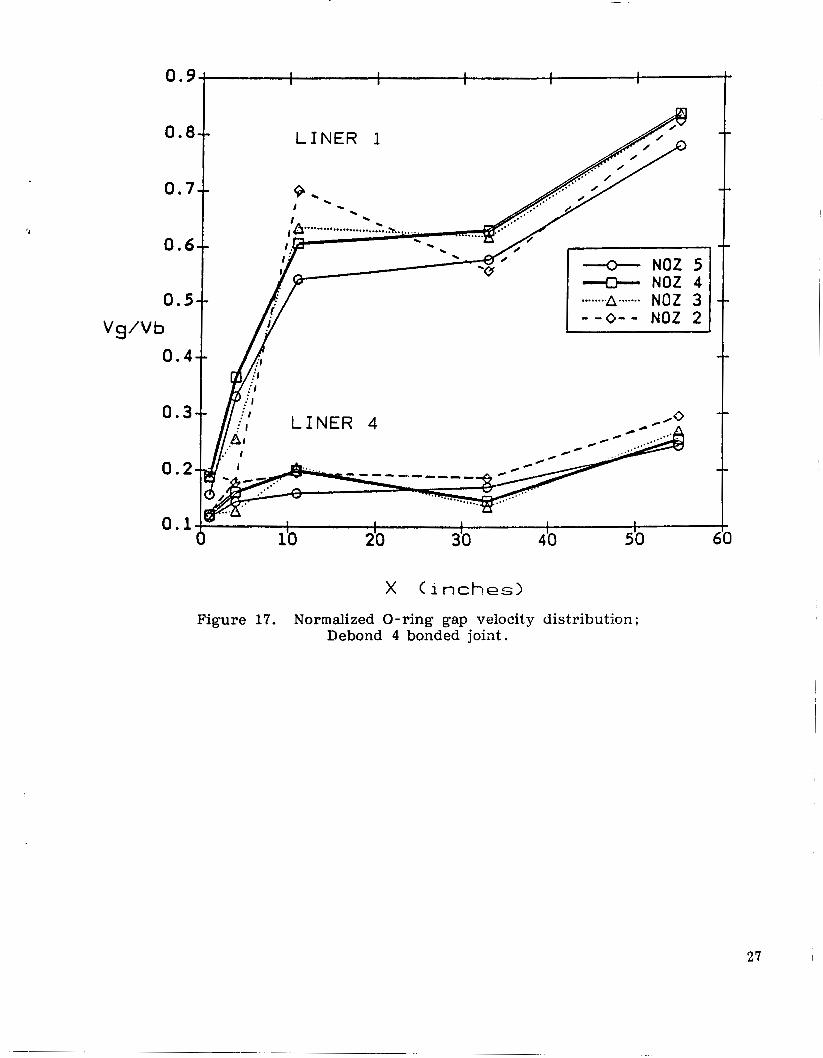
Velocity measurements in the Debond 4 joint are shown in Figures 16 and 17. Additional measurements were made in the joint entrance region at axial locations 1 in. and 4 in. from the model inlet to help characterize the inlet flow field. Figure 16 shows the axial flow build up along the gap for both the liners tested. The figure shows the initial flow acceleration, followed by an almost uniform or a slight dip in the velocity in the gap mid region, with subsequent flow buildup up to the last axial location QEF3, where data was taken. cases than for the liner 4 cases. Normalized velocities are featured in the next figure, Figure 17, which helps in the comparison of data with the vented joint and the Debond 2 joint configurations. 14, 15, and 17) brings to light the following flow behavior:

These effects are felt a lot more for the liner 1

A comparison of results from these joints (Figs.

,

8

ORIGINAL PAGE IS W POOR QUALITY

ORIGINAL PAGE IS OF POOR QUALITY

a. In the gap entrance region (location QAB3, X = 11 in.) , the Debond 4 joint has higher velocities than either the vented or Debond 2 joints. However, at the gap midpoint (X = 33 in . ) , the vented joint velocities are higher than those for the other two joints.

b. Substantial velocities are seen to occur in the gap (up to 80 percent of the bore

The figures also help gauge the impact of the gap width on the gap veloci- ties. velocity) in all the three joints being compared. Changing the gap dimension also affects the velocity profile and, thereby, will have an impact on the heat transfer characteristics of the gap region.

c. As mentioned earlier, the Debond 2 configuration shows significant end effects that are not apparent in the results for the other two joint models.

The pressure data for the two debond models tested also show the impact of the gap width on the static pressure gradient in the gap region. gradient for Debond 4 is almost 70 percent larger than that for the Debond 2 model under the nominal set of flow conditions. impact on the heat-transfer characteristics of the gap for the two debond configura- tions. transfer coefficient gradients in the gap entrance region for the Debond 4 joint than for the Debond 2 joint. This effect correlates with the steeper velocity gradients in this region (between location QAB3 and QCD3) (Figs. 15 and 17) . rate for the Debond 4 joint is thus higher in the entrance region than that for the Debond 2 geometry and about the same as that for Debond 2 in the gap mid-point region

The static pressure

This result also translates into a significant

Heat-transfer data from heat-flux gages in the gap area show sharper heat

The heat transfer

5.3 Type 2 Bonded Joint (Debonds 5, 6 , and 8)

The Type 2 debond joints simulate the adhesive flaws in the insulation gap of the SRB nozzle-to-case joint. This geometry is realized by sealing off the air flow between the model bore and the gap between the O-rings by rubber gaskets except at modeled blow-through areas. in Figure 18 along with the dimensions pertaining to the geometry in a tabular form. The air flow route in the gap area is also sketched in this figure. The simulated flaws are present both at the inlet and exit sections of the model, the gaps being equal at both ends. Three debond models, 5, 6, and 8 , w e r e tested in the present study with parametric changes of the bore inlet Mach number and the imposed axial pressure gradient. flow in the joint entrance region towards the gap between O-rings particularly when the dynamic pressure is augmented in this region by the use of restrictive liners in the model bore (greater axial pressure gradient). The flow then turns through 90 deg and is essentially parallel to the gap along its major stretch before exiting down- ward in the aft section of the simulated Baw region. The oil flow tests thus show that there is considerable kinetic energy associated with the flow as it propels upwards. After the turn in the gap between O-rings, this energy accelerates the flow in the vicinity of the closure O-ring, the exact nature of the flow field being determined by the geometry of the debond model itself. bound to separate, and, depending on where the hot wire is located in this region, one might expect either a high or a low velocity reading. Thus, the entrance region of the model is of considerable interest for the Type 2 debond configuration with the potential for the flow field to have a significant impact on the heat transfer charac- teristics in the region. The motivation to concentrate on the entrance region in the

These debond configurations are schematically shown

Prior oil flow tests revealed that their exists considerable upward

The flow rounding this sharp corner is

9

Phase 2 of operations was further strengthened from the fact that all subsequent missions would use the adhesive joint configuration in the SRB stacking process.

A s was done for the vented joint case, the effect of the gap width (Figs. 12 and 13) on the flow field was first examined. Figure 19 shows the measured velocities in the gap using liner 1 in the model bore. A s is evident from the figure, very little difference in the velocity readings is seen to exist; the differences being even smaller than those for the vented joint. bonded joints were carried out using the nominal gap dimensions (see Table 3 in Fig. 1 1 ) .

Again, all subsequent tests of the Type 2

5 . 3 . 1 Debond 5

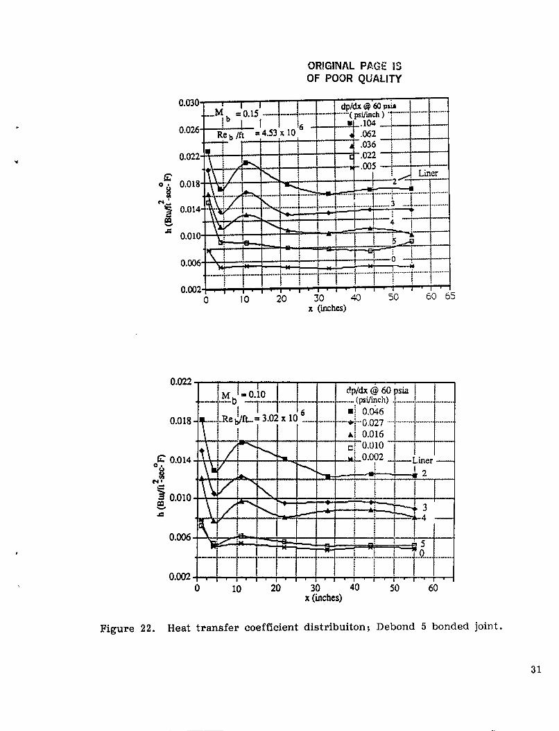
Velocity measurements for the Debond 5 geometry are presented in Figures 20 and 21 for liners 1 and 4, respectively. From Figure 20 it can be seen that there is considerable velocity at station QAB3 ( X = 11 in.) particularly at large inlet bore Mach numbers, Mb. For Debond 5 , the debond gap is only 0 . 5 in. and the velocity spikes are still evident 11 in. away on the downstream side. N o measurements were taken upstream of this location and, hence, the entrance region flow field characteriza- tion is not possible. The flow thereafter decelerates and remains almost uniform past the gap midpoint region. For liner 4 (Fig. 211, the characteristic velocity spikesseen in Figure 20 are not present, with the entire flow field being nearly uniform. N o par- ticular end effects are seen in both the figures and no significant upstream effects of the blowhole in the model aft region are seen. to see the entrance region behavior and these results are reproduced in Figure 22 from Reference 2 for two different bore entrance Mach numbers. The data corroborates the velocity information presented in Figure 20. transfer coefficient at X = 11 in . , where the velocity spikes were measured, Although the heat transfer data for liner 1 is not provided in the figure, the behavior should be similar to that seen for the other liners. Extrapolating the information from this figure, the velocity should be even higher in the entrance region ( X = 1 in . ) , than that at location QAB3 (Fig. 2 0 ) . explained by the presence of a recirculating zone in that area with smaller attendant velocities.

The heat transfer data was examined

There exists a peak in the heat

The dip present in the heat transfer data can be

The data from Figures 20 and 21 are presented in normalized form in Figure 23. Again the higher velocities nt X = 11 in. are apparent.

5.3.2 Entrance Region Flow Characterization

In Phase 2 of the investigation the Debond 8 model was first studied to charac- terize the entrance region of the flow field. For this debond model, the debond gap is 4 in . , the most severe flaw modeled. Velocity measurements were made at location U ( X = 1 in.) and at location VA ( X = 4 in.) with the hot wires positioned at dif- ferent orientations. The hot wire responds to the flow normal to it and since the flow turns in the gap entrance region, two inclination angles were examined. Case 1 , both the wires at locations U and VA were kept inclined at 45 deg to the vertical and, in Case 2 , they were positioned in the horizontal and vertical orienta- tions at locations U and VA, respectively. area of Figure 24. 1 and 4.

In

These cases are illustrated in the legend The figure also shows the data obtained in these tests for liners

10

I For liner 1, it is clear that at location U , the 45 deg orientation of the hot wire (open points) gives higher velocity than the horizontal orientation (shaded points). This difference can be as high as 60 percent as evidenced for nozzle 1. At location VA however, the vertical orientation of the hot wire (shaded points) gives marginally higher velocities (about 10 percent more for nozzle 5) than the inclined wire case (open points).

For liner 4, similarly, at position U , the 45 deg inclination gives velocities greater than that for the horizontal orientation case. inclined hot wire gives slightly higher velocity readings (about 6 percent) than the vertical orientation case. It is to be noted that location VA is at 4 in. which is also where the rubber gasket for this debond starts. Based on these observations, the velocity data at locations U and VA for Debonds 6 and 8 were obtained with the hot wires oriented at 45 and vertical, respectively. 8 are discussed in the following sections.

However, at location VA the

The velocity data for Debonds 6 and

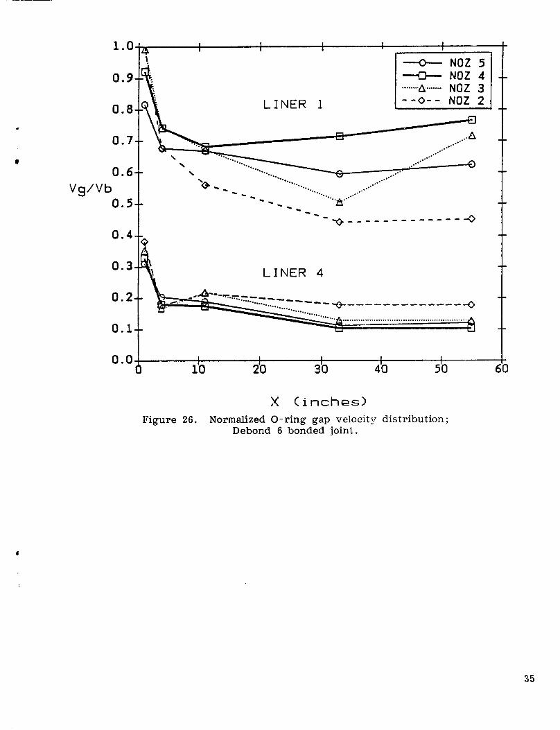
5.3.3 Debonds 6 and 8

The velocity profiles in the gap for Debond 6 are presented in Figures 25 and The following infer- 26 and those for Debond 8 in Figures 27 and 28, respectively.

ences can be drawn from the figures:

a. Velocities for Debond 6 are similar to that for Debond 5, with sharp velocity peaks in the gap entrance region. For this debond, the debond gap is 1 in. on either side and the flow exhibits similar trends for both the liner cases investigated. Also, the velocities are very close in magnitude to the bore velocities, giving the largest ratios than for any other debond tested.

liner 1 case and show uniformity past the gap midpoint for the case of liner 4. end effects are seen propogated into the flow field upstream from the rear flaw region.

b. The velocities are almost uniform past the X = 11 in. axial location for the N o

c. The heat transfer data for this debond are similar in trends to that for Debond 5 presented in Figure 22 except that it is higher in value than for the Debond 5 case. The maximum heat transfer for this case is 5 7 percent more than the maximum measured for the Debond 5 case. of 1 in. in this case than in the previous case (0.5 in.) . also show a dip at the X = 4 in. location followed by a rise at the X = 11 in. location as noticed for Debond 5 , but the velocity data do not show this behavior.

This result translates from the larger debond gap The heat transfer results

d. For Debond 8 (Figs. 27 and 28) the velocities show a reverse trend than that for Debonds 5 and 6.

debond gap is now 4 in. which is fairly large giving the flow more room in which to enter the gap between the O-rings. Again there might be regions in this flow field which have high velocities associated with them but the location of the hot wires do not capture these velocities.

In the entrance region, the velocities are low and garner This arises because the * strength farther down in the gap between the O-rings.

e. For liner 4 the flow is almost uniform except for small accelerations in the entrance region.

f . The heat transfer data for Debond 8 also shows the behavior exhibited by the flow field. The heat transfer rate is slow to start with and increases w i t h the

11

axial distance before reaching a maximum and then dropping slightly to the uniform value in the gap. This trend is again the opposite of what was measured for the Debond 5 and 6 cases where the highest heat transfer rates were measured in the entrance region.

g. The highest measured heat transfer for Debond 8 is about 26 percent smaller than that for Debond 6 , indicating that the heat transfer rate and the flow field in the debond gap are sensitive to the size of the debond gap itself. A gap of 1 in. (Debond 6) gives a higher heat transfer rate than that for a smaller gap of 0.5 in. (Debond 5) and a larger gap of 4 in. (Debond 8) . Thus, there should exist some critical debond gap dimension which yields the highest velocities and, hence, the highest heat transfer rates in the O-ring vicinity. that the most severe debond case modeled (Debond 8) is not necessarily the most severe case, erosion wise.

This then points out to the fact

6. CONCLUSIONS

Hot-wire anemometry was successfully utilized to obtain velocity data in the gap between O-rings of the 2-D SRB nozzle-to-case joint model. oped for the calibration of hot wires/films and subsequent corrections to be applied to the hot w i r e response in the data reduction stage. These corrections are required to account for changes in temperature, pressure , and probe orientation from the calibra- tion conditions. tion schemes before the final production runs were made on the model.

Procedures were devel-

Preliminary tests were conducted to verify the calibration and correc-

The generic vented joint configuration, Debonds 2 and 4 Type 1 bonded joints, and Debonds 5 , 6 , and 8 Type 2 bonded joints were successfully tested and results obtained for the gap velocity distribution for these joint configurations. was also made to characterize the flow field in the joint entrance region in the vicinity of the debonds. cant flows in the O-ring gap especially when the circumferential flow is strong and there is a substantial dynamic pressure in the joint region. between the wiper and closure O-rings can be as large as the circumferential flow velocity itself for certain debond dimensions. blow-through, builds up to a maximum value as the flaw enlarges, and then drops for larger debonds. A debond in the adhesive can thus result in large local velocities o r velocity spikes in the flaw vicinity that can have a significant impact on the joint heat transfer characteristics. the hot wires and these measurements can serve as a useful data base for numerical efforts in modeling the flow in the joint.

An effort

The data show that flaws in the insulation sealant can cause signifi-

The velocity in the gap

This f low starts out small for a small

The heat transfer data corroborated what was measured by

This effort was primarily aimed at initiating and demonstrating the use of hot wire anemometry in testing actual components o r models of flight hardware and con- siderable success has been achieved towards this objective. channels only was available for these tests and coupled with time and model constraints velocity data could be obtained at very selected locations only. The flow field, without a doubt, and only further tests can fully reveal features of the flow field and the associated turbulence levels.

4

A maximum of three

is three-dimensional in the gap vicinity, especially in the entrance region,

Integration of this technique into the regular flow measurement I sequence should prove useful in subsequent flight hardware testing and evaluation.

12

ORIGINAL PAGE IS OF POOR QUALITY

REFERENCES

1. H a i r , L. M. and McAnally, J. V . : Unheated Air Tests of SRB Field and Nozzle Joints at NASA/MSFC EAFF; SRM D MSFC Tests 22, 23. CHR/87-708, May 1987.

Pretest Information for Two-Dimensional

t

2. McAnally, J . V. and H a i r , L. M . : 2-D SRM Nozzle-to-Case Joint Test Data Report. HSC-SRB-001, NASA Contract NAS2-12037, August 1988.

3. Zaric, Z . : W a l l Turbulence Studies. Advances in Heat Transfer, Ed . Hartnett, J . P. and Irvine, T. F., Vol. 8 , Academic Press, 1972.

4. Model 1125/1125R- 1 Calibration/Probe Rotator Instruction Manual. Revision F, TSI P/N 1990133, TSI Inc., 1984.

13

TABLE 1. DIMENSIONS OF AUXILIARY ITEMS

- Id Length (") Depth Width (")

a. Debond Models (No pitot probes in slot)

-~

1 Full (65") 2 3 4

5 0.50 6 1 .oo 7 I 2.00 8 4.00

I #

.

Diameter Id Length (")$ Exit Dia. (") Ratio 1 64.12 1.006 0,050 2 62.57 1.928 0.060 3 59.39 2.250 0.070 4 52.24 2.572 0.080 5 28.97 2.892 0.090

I

dP/dx (psi/") at Bore Mash No.% .03 -05 .07 .10 .15 .0047 .0113 .0268 -- -- -0023 .0063 .0125 .0230 -- ,0012 .0034 .0066 .0137 -- .0007 .0020 .0039 .0079 .0180 -- -- .0024 .0049 .0110

b. Tapered Linerc

0.005 0.0 10 0.020 0.030

Full (0.10) I # - One at each end.

Entrance Dia = 3.214" Slot Width = 0.100"

c. Exit Nozzles

Exit Dia. (") IId I I I

I

0.732 0.944 1.1 16 1.332 1.625

L I

Bore Mach No.

0.030 0.050 0.070 0.100 0.150

.

14

*

Nozzle Id. Bore Inlet dP/dX Mach No. (psi/inch)

TABLE 2. BORE VELOCITY AND PRESSURE DATA

Bore Velocity at Stn. A (ft/s)

LINER 1

0.03 1 I 0.05 0.009 34.0 0.027 1 56.0

Nozzle Id. Bore Inlet dP/dX Mach No. (psi/inch)

2 0.05 0.002 3 0.07 0.008 4 0.10 0.0 16 5 0.15 0.035

3 4 5

Bore Velocity at Stn. A (ft/s)

56.0 78.0

112.0 168.0

0.07 0.10 0.15

0.054 0.109 0.239

78.0 112.0 168.0

i I 1 I

LINER 4

15

W

c a

F!

U 0

c E 0 7

.-

.l-l .- 0

a, rn a ? 0 c,

l a, 4 N N

2 T

%

c ho rn a,

k

.*

a 2

c, a k

16

I

ORIGINAL PAGE IS OF POOR QUALITY

a i n

W I- W I 0 K 0 mJ

0

I

a \ \

a 4 a,

c-’

.Fl c 0 .- a, CT) cd 0

0 I

+ l

a, 4 N N : a P= cn

a c E

17

I c o 2 W d 2

c U

f a

i 0 L

3

&

P

d

&

.

18

ORIGINAL PAGE IS OF POOR QUALITY

q E

p fl fsr c y

il E b

8 3

ii ii

k 0 03 +J k P cd u

.r( +

a, 5 cu 0

u .d u cd

a c cd

a, P

PI E

a,

bn cr .?I

19

16

HOT W I R E PROBE 1210-TI-5 14

12

10

0

6

4

2

0

T = 6 9 . 5 deg F

"0.5

E *

Figure 5 . Hot wire calibration using the TSI calibrator.

'b

(f t/s)

Distance ( f r o m station A )

Figure 6. Bore velocity distribution during the HWA calibrations.

20

Channel 1

6.0

5 . 5

5 . 0

4 . 5

E Z 4 .0

3.5

3.0

2 . 5

2.0

1

E * 0.36698 Yo.’ + 1.13777, T = 5 5 ’ F

“ 0 . 5

n L Figure 7 . Hot wire anemometer calibration, Po = 60 lb/in. .

Channel 2

6.C

5.5

5 . 0

E * 4 . 5

4 . 0

3 . 5

3.0

1 I I _t___

/ E’ 0.40948 Yo” + 1.04118, T I 5 5 ’ ~

/ i’

/

0 . 5

Figure 8 . Hot wire anemometer calibration, Po = 60 lb/in. 2 .

21

Channel 3

"0.5

2 Figure 9. Hot wire anemometer calibration, Po = 60 lb/in. .

IA r 5/8-18NF-2A r 0.625"

< 1 .750"

S E C T I O N A-A

D R I L L & 'TAP fo r

1 /8"NPT

Figure 10. Machined plug for holding the hot wires.

22

Dimensions 7-

Dimension (inches) minimum 1 nominal I max I mum

I I I

Gap 1

Gap 2 0.042 0.046

Gap 3 1 0,042 1 0.046

Gap 2

0,050

0.050

Gap 3

Wiper 0-r i ng

Table 3 :

I 0.002 1 0.006 I 0.010 I

L I I I I

- Gap 1

- Gap 2

- Gap 3

Figure 11. Geometry of the gap between the O-rings.

23

100 i 1 I I I I I I I

I I

I ' I

8ot 60 '4 NOZ 4

...................... ....................... 0 ............ ... 0-

rn u ; ...................... 0 ...................................... B .......................

I I I I I I I 2b 30 4b 50 10 '

1'0

X (inches)

,

I

Figure 12. Effect of gap width; velocity data in the vented joint, liner 1.

(f t / s ) T

n c 30 t NOZ 5

... r N O Z 4 t ,.a,.

40

CIC V 9

ZU

15

10

t I

X (inches)

Figure 13. Effect of gap width; velocity data in the vented joint, liner 4.

24

0.4--

0.3--

0.2--

0.1--

1.0

L I N E R 1

0.3--

0 . 2 - -

0.1--

t L I

A

NER 4

- - -0 - - - ....... .... A,.. ................

n

/ ,:' .... .................................. , .

-

0.0 ' , I I I I I

lb 20 310 410 5'0 60

X (inches)

Figure 14. Normalized O-ring gap velocity distribution; vented joint.

L I N E R 1

0 0 '., \

...... .... ....................................... / , ,..D ..&-

LINEF; 4 .... .....

'

I I I 4 I

510 0.0 I 1'0 2b 3b 410

X (inches)

I

Figure 15. Normalized O-ring gap velocity distribution; Debond 2 bonded joint.

25

100

(f t/s) 75

50

- _ _ _ -

- . - . - . - , - v.-'-' _ . - ' 25 : I ,a,-.- . _ . _ , _ .

50 t T I '

I I I I I I 1'0 20 30 4 0 50 60

0'

X Cinches)

L INER 4

t I ' I

45 t t V 9 t/s> (f

15 ..... ....

0 , I I I I c 10 210 30 40 50 60

X (inches)

Figure 16. O-ring gap velocity distribution; Debond 4 bonded joint.

I

0.

0.

0.

0. V g / V b

0.

0.

X (inches)

Figure 17. Normalized O-ring gap velocity distribution; Debond 4 bonded joint.

t

0

E

ORIGINAL PAGE IS OF POOR QUALITY

loo t I 1 I 1 1 I I I I I I I

901 80

LINER 1

a

"9 ( f t / s > 50

40 t

lot I I I I

1'0 2'0 310 4 0 50 I40 0

X (inches)

Figure 19. Effect of gap width on the gap velocities; Type- 2 bonded joint.

60

50

(f t/s> ::I 20 ...

......... '.. ... ... \ ~

a...

'.. ... ... . .... . . '.. . a,.-.. .......... . . . ......................................... s . . a

A.

.a - - - - - - - -A -.-.-0

V

- - - - - - -.-_ -.-. - . - . _ -.-. _ _ - , _._. - .-. -0. - .-_

_,._..-.. -B.. ..._.,

-..-_._ -._ -..- . -.. -.-.._.. -..._ _,,_.. _._-..-' a .-..-'.-''

I I I I I I

1'0 2'0 310 4 0 5b 610 10 ' X (inches)

Figure 20. O-ring gap velocity distribution; Debond 5 bonded joint, liner 1.

29

6C

50

40

"9

30 (f t/s)

20

10

0

LINER 4

I I 4 I I

lb 2b 3b 4b 5b

X (inches)

Figure 21. O-ring gap velocity distribution; Debond 5 bonded joint, liner 4.

I 30

ORIGINAL PAGE lis OF POOR QUALITY

5 x (inches)

0.022

0.018

0.014

(Y'

5 0.010 p1 v c

0.006

0.002 0 10 20 30 40

x (inches) 50 60

Figure 22. Heat transfer coefficient distribuiton ; Debond 5 bonded joint.

31

- - - - - _ -

. . . - --*. . ......................................................... A ..._,_ .'...

0.3--

0.2--

0.1--

0.0 I I I I I

X (inches)

--

--

--

Figure 23. Normalized O-ring gap velocity distribution ; Debond 5 bonded joint.

32

14-

"9 <f t/s)

12-

10-

I 1 I I

0 LINER 1 o

I 16t 0

LOC. u

- 8

V

LOC. VA

0

i" 8

t'" t

4 3 10 k

X (inches)

I 16 I I ' 35

LOC. u LOC. VA

"9 "t : (f t/s> 3

lot

30

25

A A v V

I 1

i 1 3 4 5 X Cinches)

'5 k

LEGEND

o 0 NOZ 5 0 NO2 4 A A NOZ 3 o NOZ 2 V V NOZ 1

Case 1: O p e n Pts.

-Lc- -- Model B o r e

C a s e 2: Shaded P t s .

-- r4odel Bore

Figure 24. Effect of probe orientation on the gap velocities; Debond 8 bonded joint.

33

"9 (f t/s>

......... ..... ......... ...... ..... ....... ..... .........

* - - - - - - - - - - _

....... ..... ..........

,&-.

- - 0 - - -

...... A .._..' ........... ...... ..... . . .

I I I I 1 I 1'0 20 30 4 0 50 6'0 01

X (inches)

LINER 4 .... A . . NOZ 3

10 I

1- 0 I

I I I lb 2'0 30 4'0 5'0 6b

X (inches)

Figure 25. O-ring gap velocity distribution; Debond 6 bonded joint.

I 34

1.

0.

0.

0.

0. V g / V b

0.

0.

0.

I 1 I I I I

4 to LINER 4

-0

0.0 I I I I I I

1'0 2'0 3b 410 510 60

X (inches> Figure 26. Normalized O-ring gap velocity distribution ;

Debond 6 bonded joint.

35

t 150 I I 1 I 1

I I 1 I I I

1-0- NOZ 511

1 I I I 1

I 0

"9

1 I I I 1

I 0

LINER 1 125

1 , I I 1

lb 2b 30 410 5b 6b 0'

X (inches)

I LINER 4 .......A ....... NOZ 3 I -

36

I

i i

i i

0 . 8 O o 9 !

-11 ......_.A .......

- -0- - NO2 2

0.6t

V g / V b 0 . 5 1

0 . 4 t

LINER 1

LINER 4 0.3

0.2

0.1

0 . 0 I 1 1 t 1 1 110 210 310 4b 5b 6b

X (inched Figure 28. Normalized O-ring gap velocity distribution; Debond 8 bonded joint.

37

T E C H N I C A L R E P O R T S T A N D A R D TlTLE P A G l 1. REPORT NO. 12. G O V E R N M N T ACCESSlON NO. 13. RECIPIENT'S CATALOG NO.

CR- 183528 I 4. T I T L E AND SUBTITLE 5 . REPORT DATE

Hot Wire Anemometer Measurements in the Unheated Air Flow Tests of the SRB Nozzle-To-Case Joint 6. PERFORM,NG December ORGANIZATION 1 9 8 8 CObE

Universities Space Research Association 4950 Corporate Drive, Suite 100 Huntsville, Alabama 35806

7. AUTHOR(S)

N . Ram- 9. PERFORMING ORGANIZATION NAME AND ADDRESS

1 1 . CONTRACT OR GRANT NO.

NAS 8- 36474 (3. TYPE OF REPOR'I' & PERIOD COVEREC

8. PERFORMING ORGANlZATlON REPORT A

( 0 . WORK UNlT NO.

12. SPONSORlNG AGENCY NAME AND ADDRESS

National Aeronautics and Space Administration Washington, D . C . 20546

7. KEY WORDS 18. DlSTRlBUTlON STATEMENT

F i n a l Contractor Report

1.1. SPONSORING AGENCY CODE

Hot-wire Anemometry Nozzle-to- Case Joint Debonds Circumferential Flow

9. SECURITY CLASSIF. (d thh meart) 20. SECURtTY CLASSIF. (olthf. pi.) 21. NO. OF PAGES

Unclassified Unclassified 4 4

Unclassifiea - Unlimited

22. PRICE

NTIS