Embed Size (px)
Citation preview
SRD- 147 127 CURRENT PROBLEMS IN TURBOMACHINERY FLUID DYNAMICS(U) /2MASSACHUSETTS INST OF TECH CAMBRIDGE GAS TURBINE ANDPLASMA DYNAMICS LAB E M GREITZER ET AL. JUN 84
UNCLASSIFIED FOSR-TR-B4-B859 F49620-82-K-B2 F/G 20/4 NLIEIIIIEIIIIIEIIIIIIIIIIIIIuIIIIEEIIEIIEIIIEEIIIIIIIIIEEEEEIIIEEEEEEIIE/IEE//EE/IE
-.-. -i,*..- ." • • -.
l::i
I
oK /
L602 1250
": II~~~~~~~IIIII ' 2o; .. ? '
:; ~~~IElll ' .-.-" . 1V8i! IIII1 L.-'4 J7"
.. . .. . . . . . . . . . . . . .:..
fil
t-'-~~11115
i V
R 1
rt
* UNCLASSIFIEDSECURITY CLASSIFICATION OF THIS PAGE
REPORT DOCUMENTATION PAGEI&. REPORT SECURITY CLASSIFICATION 1b. RESTRICTIVE MARKINGS
UNCLASSIFIED2.& SECURITY CLASSIFICATION AUTHORITY 3. DISTRIBUTION/AVAILABILITY OF REPORT
________________________________Approved for Public Release;2. OECLAS5IFICATION/DOWNGRADING SCHEDULE Distribution unlimited.
4. PERFORMING ORGANIZATION REPORT NUMBER(S) B. MONITORING ORGANIZATION REPORT NUMBER(S)
MIT Gas Turbine Laboratory Report No.
G&. NAME OF PERFORMING ORGANIZATION b, OFFICE SYMBOL Ta. NAME OF MONITORING ORGANIZATION
MASSACHUSETTS INSTITUTE OF ir (Ippliea) Se#TECHNOLOCY I_31264 _______________________
6c. ADDRIESS (City. Stat. and ZIP Code) 7b. ADDRESS (City. State and ZIP CodrlD)EPARTMENT OF AERONAUTX.S & ASTRONAUTICSCambridge. Massachusetts 02139 Se0
21. NAME OF FUNDING/SPONSORING -]Sb. OFFICE SYMBOL 9. PROCUREMENT INiSTRUMENT IDENTIFICATION NUMBEROIRGANIZATION AIR FOR 'CE (fapial) Contract No. F49620-82-K-0002
OFFICE OF SCIENTIFIC REAACH AVFOSR/NA
Sc. ADDRESS (City. State and ZIP Code) 10. SOURCE OF FUNDING NOS.
PROGRAM IPROJECT TASK WORK UNITAFOSR /NA ELE ME NT NO. NO. NO. NO.Bolling Air Force Base, D.C. 20332 61102F 2307 A4
11. TITLE (include Security Classification)
lurrent Problems in Turbomachinery Fluid Dynami s (UNCLASSI1 IED)12. PERSONAL AUTHOR(S) U~b LaHE.M. Greitzer, J.L. Kerrebrock, W.T. Thompkins, Jr., J.E. McCune, A.B. Epstein, W.R. Hawthor e13&. TYPE OF REPORT 13b. TIME COVERED 14. DATE OF REPORT (Y.. Mo.. Day) 15. PAGjE COUNTSemi-annual Report FRO 1118 o4//8 7/16/84 10L
16. SUPPLEMENTARY NOTATION
17. COSATI CODES I S. S UBJE CT T ERAMS (Con tinur on revierse it necee.,- and iden tify by block num bar)FIELD GROUP SUB. GA. Transonic Compressors, Compressor Stability, Casing
Treatment, Inlet Vortex, Design, Heavily Loaded Comn-pressors
19. ABSTRACT (Continue on nru.,.. it nece~uauv and identify by block number)
-A multi-investigator program on problems of current interest In turbomachinery fluiddynamics is being conducted at the MIT Gas Turbine and Plasma Dynamics Lab, Within thescope of this effort, four different tasks, encompassing both design and off-designproblems, have been identified. These are: l)Investigation of fan and compressordesign point fluid dynamics (including formation of design procedures using current three-dimensional trarjsonic codes and development of advanced measurement techniques for use intransonic fans); 2)Studies of basic mechanisms of compressor stability enhancement usingcompressor casing/hub treatment; 3)Fluid mechanics of inlet vortex flow distortions ingas turbine engines.11 2 )Investigations of three-dimensional analytical and numerical com-putations of flows in highly loaded turbomachinery blading.pL-,n addition to these tasks,this multi-investigator effort also includes the Air Force ftesearch in Aero PropulsionTechnology (AFRAPT) Program. This document describes work carried out on this contract ..
during the period 11/1/83 - 4/30/84.20. DISTRIUUTION/AVAILABILITY OF ABSTRACT 21. ABSTRACT SECURITY CLASSIFICATION
UNCLASSIFIED/UNLIMITED 10SAME AS RPT. 0 DTIC USERS 0 UNCLASSIFIED
22s. NAME OF RESPONSIBLE INDIVIDUAL 22. TELEPHONE NUMBER 22c. OFFICE SYMBOL
James D Wilson20/6-95AORNDO FORM 1473. 83 APR EDITION OF I JAN 73 IS OBSOLETE. UNCLASSIFIED
SECURITY CLASSIFICATION OF THI1S PAGE
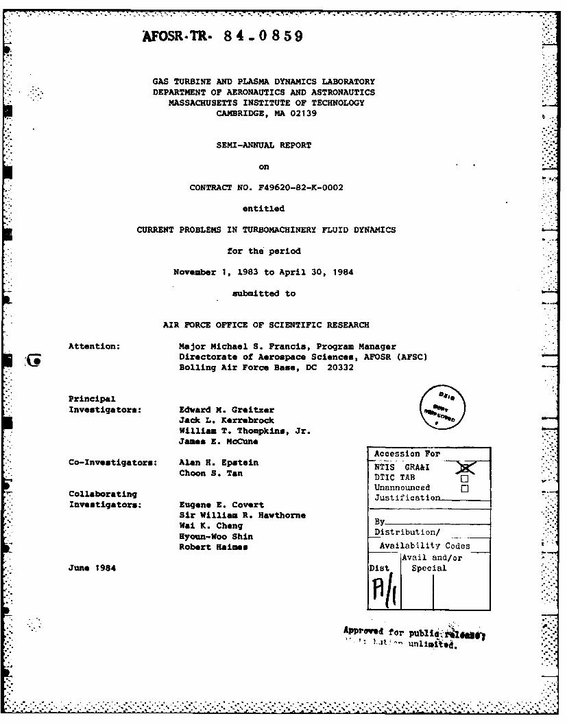
AFOSR-TR. 8 4.0 85 9
GAS TURBINE AND PLASMA DYNAMICS LABORATORYDEPARTMENT OF AERONAUTICS AND ASTRONAUTICS
MASSACHUSETTS INSTITUTE OF TECHNOLOGYCAMBRIDGE, MA 02139
SEMI-ANNUAL REPORT
on
CONTRACT NO. F49620-82-K-0002
entitled
CURRENT PROBLEMS IN TURBOMACHINERY FLUID DYNAMICS
for the period
November 1, 1983 to April 30, 1984
submitted to
AIR FORCE OFFICE OF SCIENTIFIC RESEARCH
Attention: Major Michael S. Francis, Program ManagerDirectorate of Aerospace Sciences, AFOSR (AFSC)
C* Bolling Air Force Base, DC 20332
PrincipalInvestigators: Edward M. Greitzer 14160
Jack L. KerrebrockWilliam T. Thompkins, Jr.James E. McCune _____
Accession ForCo-Investigators: Alan H. Epstein --NTIS GRA&I
Choon S. Tan DI A
* CollaoratingUnannounced ICollboraingJustii'icatio
*Investigators: Eugene E. CovertSir William R. HawthorneVai K. Chong By
Hyoun-Woo Shin Dsrbto!____Robert Haimes Availability Codes
'vail and/orJune 1984 Dist Special
APPrmvd for public'Z'memiunlimitea.
TABLU OF CONTENTS
1INTRODUCTION AND RESEARCH OBJECTIVESI
2.WORK To DATE AND STATUS OF THE RESEARCH PROGRAM ~ 2Task I: Inlvestigation of an and CompressorDesign Point Fluid Dynamics
2A- Inverse Design Task
2B. Loss Mechanisms and Loss Migrationin Transonic Compressors
32Task II: Compressor Stability Enhancement UsingHUb/Casing Treatment
38Task III: Inlet Vortex Flow Distortions i a ubnEngines i a ubn
43Dimensional Flows in Highly Loaded Turbomachines 82
A. 3D Flow anld Design Methods In Highly.LoadeTurbomachines
82B. Numerical studies ofSecondary Flow in aBend Using Spectral Methods
8C* TreeDimnsin&IBlade Design forLarge Deflection
90General Progress On AFRAPT
93. PUBLICATIONS
94. PROGRAM PERSONNEL
985. INTERACTIONS10
6. DISCOVERIES AIR FROTFT 07 SCT1WT!ylC REStLR'. (AYSC) 107. CONCLUSIONSOII~CZ~
~ ~ OtI 101
MATTHEW ~ ' 4 ~Kappf srnoe Iatwstouiiuo
Distrib.iti..
a.'H .. .. .M
C4et "I'rcs * rtL,,DTIL1
..::
1.* INTRODUCTION AND RESEARCH OBJECTIVES
This report describes work carried out at the Gas Turbine and PlasmaDynamics Laboratory at MIT, as part of our multi-investigator effort oncurrent. problems in turbomachinery fluid dynamics. Support for thisprogram is provided by the Air Force Office of Scientific Research underContract Number F49620-82-K-0002, Major M.S. Francis and Dr. J. D. Wilson,Program Managers.
The present report gives a summary of the work for the period 11/1/83 - .4/30/84. For further details and background, the referenced reports, pub-lications and previous reports (covering the period 10/1/79 - 5/31/83)1,2,3,4should be consulted.
Within the general topic, four separate tasks are specified. Thesehave been described in detail in Reference 1, but they are, in brief:
1. Investigation of fan and compressor design point fluid dynamics,
2. Studies of compressor stability enhancements,
3. Fluid mechanics of gas turbine operation in inlet flow distortion,
4. Investigations of three-dimensional flows in highly loadedturbomachines.
In addition to these tasks, the multi-investigator contract alsoencompasses the Air Force Research in Aero Propulsion Technology
program. The work carried out in each of the tasks will be described in -.-
the next section.
References
1. E.M. Greitzer, et al., AFOSR TR-82-0027, Final Report, 10/79 - 9/81,on "Current Problems in Turbomachinery Fluid Dynamics."
2. E.M. Greitzer, et al., Annual Report, 10/1/81 - 11/30/82, on "CurrentProblems in Turbomachinery Fluid Dynamics."
3. E.M. Greitzer, et al., Semi-Annual Report 12/1/82 - 5/31/83, on"Current Problems in Turbomachinery Fluid Dynamics."
4. E.M. Greitzer, et al., Annual Report, 12/1/82 - 10/31/83, on "CurrentProblems in Turbomachinery Fluid Dynamics."
Ze..-....
* .. - . .. .. . % '**.*,****~. %**.*.*.**.*.*.**.~.*.-.. .. - ... -. '- ..- -... .. .. ,°o.'
2
TASK I: INVESTIGATION OF FAN AND COMPRESSOR DESIGN POINT FLUID DYNAMICS
TASK IA: INVERSE DESIGN TASK
During the last three years, efforts on the inverse design project
have been directed to finding an acceptable inverse method which was appli-
cable to the full Mach number range encountered in high speed axial
compressors. We have found one method, based on time marching solutions to
the Euler equations, which is accurate enough and could potentially be
* extended to three dimensional geometries, see references [1.1], [1.2],
[13] 1.4]. This method operates in a mixed mode format in which either
* blade pressure distributions or geometric constraints are specified. The
method is unfortunately far too slow, in terms of computer time usage, for
practical design work and in its present form does not properly adjust
* solid wall positions in subsonic flow regions.
Work on the time marching like method is now considered complete with
the publication of a Ph.D. thesis on the method by Tong. This thesis
contains new information about sources of numerical errors in finite
* difference solutions and artificial smoothing operator., a demonstration
* that the simple inverse scheme would work in supersonic flow but not in
mixed subsonic-supersonic flows, and a survey and evaluation of existing
inverse and design methods.
A new direct or inverse method is now being developed which is many
times faster than the old time marching scheme, is easily coupled to
* boundary layer solvers and is more accurate than the time marching style
solver. This new method appears to retain all the traditional advantages
of streamline curvature schemes while being useful for subsonic, supersonic,
S~. . . . . . . . . . . . ., .
3
transonic, and shocked flows. The scheme can be described am a conserva-
tive finite volume scheme in streamline coordinates and has been applied to
supersonic duct flows, subsonic and transonic duct flows, subsonic cascade
flows, and viscous-inviscid interactions.
An AIAA paper, number 84-1643, was presented at the-June 1984 Fluids
meeting in Snowmass, CO. This paper presents theory, relaxation methods,
and test examples for the inviscid applications. This paper is reproduced
as Appendix I.- A peper on the viscous-invicid interaction aspects of the
work has been accepted for the Third Jymposium on Numerical and Physical
Aspects of Aerodynamic Flows in Jan. 1985 at Long Beach, CA. An internal
memo which shows the present state of the coupling work is included as
Appendix 2.
**** *' .~ q . C . . ,- . . .
4 ." ..-.... ;4
APPENDIX 1
0p
AIAA-84- 1643Conservative Streamtube Solutionof Steady-State Euler EquationsM. Drela, M. Giles andW. T. Thompkins, Jr.,Massachusetts Institute ofTechnology, Cambridge, MA
A1AA 17th Fluid Dynamics,Plasma Dynamics, and
Lasers ConferenceJune 25-27, 1984/Snowmass, Colorado
For permission to copy or republish, contact the American Institute of Aeronautics and Astronautics1633 Broadway, New York, NY 10019
-- - -
CONSERVATIVE STREAMTUBE SOLUTION OFSTEY-STATE EULER EQUATIONS
Mark Drela*Massachusetts Institute of Technology
Cambridge, Massachusetts
Mizhael Giles#
Massachusetts Institute of TechnologyCambridge, Massachusetts
W. T. Thompkins. Jr."Massachusetts Institute of Technology
Cambridge, Massachusetts
Abstract transonic full potential equation.
This paper presents a new method for solving An older approach to solving the subsonic Eule"the steady state Euler equations. The method is equations is the streamline curvature method whichsimilar to streamline curvature methods but has a can be considered to be an iterative relaxationconservative finite volume formulation which ensures solution to the equations of motion in intrinsiccorrect shock capturing. Either wall position or coordinates [2,3,4]. In one version [2] an initialwall pressure may be prescribed as boundary con- set of streamlines is guessed and the stead%-stateditions, permitting both direct and inverse calcu- normal momentum equation is integrated in the normallations. In supersonic applications the solution direction assuming known enthalpy and entropyis obtained by space-marching while in subsonic and variation along each streamtube. The resultingtransonic applications iterative relaxation methods error in the continuity equation then drives a re-are used. Numerical results are given for: laxation procedure to move streamlines towards theira) Supersonic diffuser with oblique shocks correct positions. Because it is based upon thea (Direct calculation) w steady state equations, the relaxation procedure in
the hyperbolic supersonic region must be differentb) Supersonic jet entering still reservoir from that in the elliptic subsonic region.
(Inverse calculation)c) Subsonic bump in a channel with 25% blockage One main advantage of the streamline curvature
(Direct and inverse) method is that it is much faster than time-marchingSubsonic high-work turbine cascade methods, and this makes it much more suitable for(Direct)(Diect design applications in which many different aeo-
e) Transonic bump in a channel with 12% blockage desin appicto in which a de re ntgenmetries need to be analyzed. A secondary advantageis the simple inviscid treatment of adjacent stream- '.'.
tbswith differing stagnation properties. InIntroduction time-marching calculations numerical dissipation
smears the discontinuities.At present most methods for the numerical cal- s r e c i t
culation of steady-state transonic solutions of the The major disadvantages of the standard stream-Euler equations are based upon a conservative finite line curvature method are that the iterativevolume approximation to the unsteady equations of lerare untbleain th sue icere
solvers are unstable in the supersonic regions, andmotion [ll. This approach is conceptually straight- they do not conserve momentum globally, so that forforward since the unsteady equations are hyperbolic example the lift on an airfoil may not equal thein time and so the same numerical procedure can be change in momentum of the fluid. in subsonic casesused in regions where the flow is locally subsonicor supersonic. Using a conservative finite volume thi momentum loss tcases there may be an appreciable momentum loss atformulation also guarantees the correct Rankine- the shock. Studies by Salas et al [5] of solutionsHugoniot shock jump relations regardless of the to the full potential equation show that momentumdetails of the shock calculation. loss even at relatively weak shocks can produce
The principal disadvantage of this approach is large errOrs in shock position.that the convergence rate is limited by the rela- The method we have developed is similar to theThmiecaue method , bue haedvaoe s sia tonsrvtivh:tively slow propagation of w&velike disturbances svethroughout the domain and their reflection at the finite volume formulation which ensures the correct 'boundaries of the computational domain. Current treatment of shocks. Like the streamline curvaturemethods try to overcome this limitation by a variety method it solves the steady-state equations and so --
of acceleration methods such as variable time steps, requires different solvers or solution algorithmsN' implicit operators with larger time steps, and
multiidoperatrs with larger time stepsc r gds, for purely supersonic, purely subsonic or transonicultiqr d with larger time steps n coarser grids, problems. The supersonic solver marches in stream-
but computation times remain an order-of-magnitude wise steps downstream from a known inlet flow. The ..-
larger than for the solution of the steady-state subsonic solver starts from a guessed set of stream-
*Research Assistant, Dept. of Aero and Astro line positions, solves each streamtube problem as a
#Research Assistant, Dept. of Aero and Astro separate quasi I-D problem, and then relaxes allStudent Member AIA the streamline positions to satisfy pressure con-
tinuity across streamlines. The transonic solver@Associate Professor, Dept. of Aero and Astro is similar to the subsonic solver but requiresMember AIAA numerical dissipation in the supersonic region, and
Cep l'" k-) Awavkso low'"uge of Awrumulks madApiseeIjCI. Inc.. 14. AN fIts mmuwe
.......... . ,
relaxes one streamline at a time instead of all y Pl 1 2 !. P 2 1 2simultaneously. At the present time the supersonic -1 P + T q Y-1 C _ 2 q 2 (2c)
and subsonic solvers are both robust and very fast, 1 2
but the transonic solver requires further improve-ment in calculation times. From the earlier assumption that the pressure
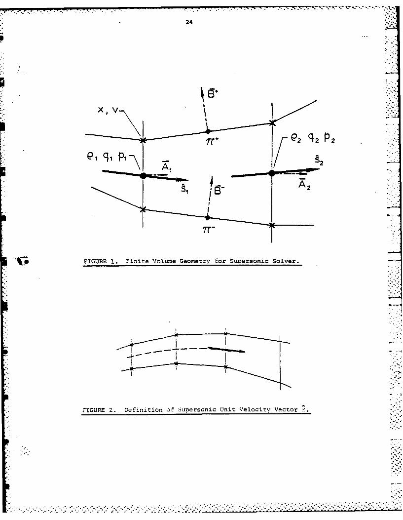
is linear over the cell, it follows that the averageFinite Volume Formulation for Euler Equations pressures on the cell faces must be related by
The governing equations are derived from the P1 + P2 - 1T
+ + IT- (2d) .
integral form of the mass, momentum, and energy
consrvaton lws.The assumption of no convection across thestreamline cell faces means that the grid is not
qndg 0 (la) known a priori. The grid geometry must then betreated as an unknown which is determined as part
0(q.n)q + pnd = 0 (ib) of the solution. This is a novel feature for afinite volume scheme, although it has long been
0(q.n)H dt = 0 (1c) used in streamline curvature schemes. This feature
also makes the inverse and direc, problems opera-where the integration is round a closed curve. tionally equivalent. In the direct problem, a
fixed wall position is imposed as a boundary con-These conservation equations are applied to dition and the wall pressure is obtained as a re-
streamtube conservation cells which have the pro- sult. In the inverse problem, the wall pressureperty that there is no convection across cell faces is prescribed as the boundary condition and thealigned with the flow (Figure 1). Density P and geometry is calculated as the result. Examples ofspeed q are defined to be the average values on both types of calculations will be given later.the faces at the two ends of the conservation cell.Also, the pressure in the cell is assumed to belinear and defined by the average values on thefour faces. For clarity, the average pressures onthe end faces are denoted by p, and on the stream-- - - -
L line faces byl. n T
strearrwise faces 02
- - -, 9, .,
LW2 9, Figure 2. Geometry definitions for streamline"2 2-.curvature equations
The momentum equation (2b), which is a vectorequation, will now be shown to reduce to the set ofA 2 streamwise and normal momentum equations used by
the streamline curvature methods, provided ourcoordinates, like the s-n coordinatel, are4 ortho-gonal. More precisely, the vectors S and N joiningthe cell midpoints in Figure 2 must become perpen-dicular and the angles e and e , between 9 and S1
Figure 1. Typical conservation cell and _ respectively, musi vanisg as the grid is2
refined. BX taking the dot product of (2b) in turnwith I and N and using (2d), we obtain the following
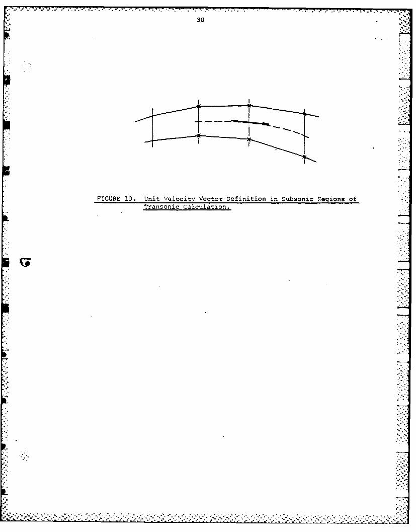
The flow direction at the end faces is given by streamwise and normal momentum equations,the unit vector i which is defined by the local
geometry. The definition of i in terms of the 2 2 -)21P q 2( i 2 .A ) (; , .S ) q ( Al )' . l i S ).
local cell node positions will be given later. The P 2 2 1 1vectors A and Bin Figure 1 are the cell face areanormal vectors. - NxSI -p-, (3a)
With the simplification that there is no con- 2 2P 2 .q2(2A 2 H ( 2 N P p1q 1( 1.*A 1 )i (s1 N)vection across the streamline faces, the discrete llS'l -
conservation equations for mass and momentum are: - I (fl9. - f-) (b.
Now define m = lq1 (s 1 ) P2q2(s2 ,A2 ). .-
pi A1 + (01ql 1 A1 )ql1 + i B- With the condition that I and i are orthogonal,and with the small angle approximations' sin =.
P2A2 + (P2q2s 2 A2 )q2a2 + 11 B (2b) and cos -1, equations (3a) and (3b) reduce to
Since the mass flux is constant along the m q2 " 2 1 4a)streamtube, the enthalpy conservation equation re- T F - - Te-duces to the simple statement that total enthalpyis constant along a stremtube.
¢. . " _7
-e ,Since the streamwise position of the normal- (4b) grid lines is arbitrary, some constraint on this
ITNi F -W streamwise position must be imposed. At present,the supersonic solver fixes the x positions for
In the limit as the grid is defined, these simplicity, leaving only the y's as geometric un-finite difference equations become the streamline knowns. A more general grid structure will becurvature equations treated in the subsonic solver section.
5q - - " (5a) At the inlet boundary all the variables are
specified. At the top and bottom boundaries oneboundary condition is specified. This boundary
q2 CP (5b) condition can be either a specified wall positionTs a-n (direct case) or a specified pressure (inverse
case). with these prescribed boundary conditionsThus our equations can be interpreted as dis- the solver marches downstream from the inlet,
crete representations of the streamline curvature solving all of the equations at each streamwiseequations. The essential point however is that our station by using an aprpoximate Newton-Raphsonconservation form ensures that shocks will be linearization of the equations. This procedure iscorrectly captured. Since equation (2d) was similar to Keller's Box Scheme [6] for the solutionnecessary to obtain the above result, it is inter- of the boundary layer equations.preted as a consistency condition on our finitevolume equations. To reduce the number of unknowns, 02 and p, are
eliminated using the enthalpy equation (2c) afdSolution Procedure for Supersonic Flow the pressure relation (Zd). With these substitu-
tions the equations for mass and momentum conser-For flow which is known to be supersonic vation are,
everywhere, a simple space-marching solution pro-cedure may be used which takes full advantage of Massthe hyperbolic character of the steady stateequations. In this solver the unknown geometry yq s (y + y -) (1+ +-Pvariables x,y are located at the nodes of the con- 2 2 2 2servation cell as shown in Figure 3a. The i unit R 2 - - 0 (6m -vector giving the local flow direction is defined (Y-1)(H - q 2 /2)
to be tangent to the circular arc passing throughthe three upstream midpoints as illustrated in x-momentumFigure 3b. This definition was chosen so that s +depends solely on upstream information, which is Rx m q2s2 )-Y + 2+
the correct domain of dependence for supersonic x xflow and allows a space-marching solution + -procedure. II (Y2 -yl) + f-(yl-y 2 ) = 0 (6b)
y-momentisn
R m(q s q s + )+(F -+ T)(x 2 -x1 ) " 0 (6c)y v
In these equations m is the mass flux which is
constant for a given streamtube. s, and s are ".
c 'y the components of the i vector. The equations are
cal linearized to calculate the corrections needed todrive the residuals to zero.
MassFigure 3a. Geometry variable locations for
supersonic solver -R R aR +6q m 6n- + +
q2 2 - +
y + M6- + Md R(7a)
circular arc Y a 2-y+ y 2 -Rtr lg ace
mridposs '2 2
S2 x-momentum
;R"- aR%%x 6 + x s.l +Y; aq2 2+
aR aR
Figure 3b. definition for supersonic solver 6y 2- + x 6y2+ - (7b)
JI J.. ° ..
S%. ...... ............. . . .. ... . -. -e. . , . ... . . . . . .-. ... ', - - .- . . . . - , - ,. . . . . . . . . . . . . ., ,
8 <v.-...
8
y-moznentum
3R aR aRS6q- + y 6n+2 " 311- an+ '"
aR IR t.+--Y;y: + 2 - R (70 .-
Equations (7a-c) for each streamtube cell areassembled in a 3x3 block tridiagonal form togetherwith the two boundary conditions, and are solvedby standard methods. Because the equations arefully linearized, this Newton-Raphson procedure re-quires only three or four iterations at each stream- "-'--...-.- -'wise station to converge machine accuracy. i and 'V* -->, . :'"' -
p, can then be calculated from the enthalpy nd ,., . ,energy equations.
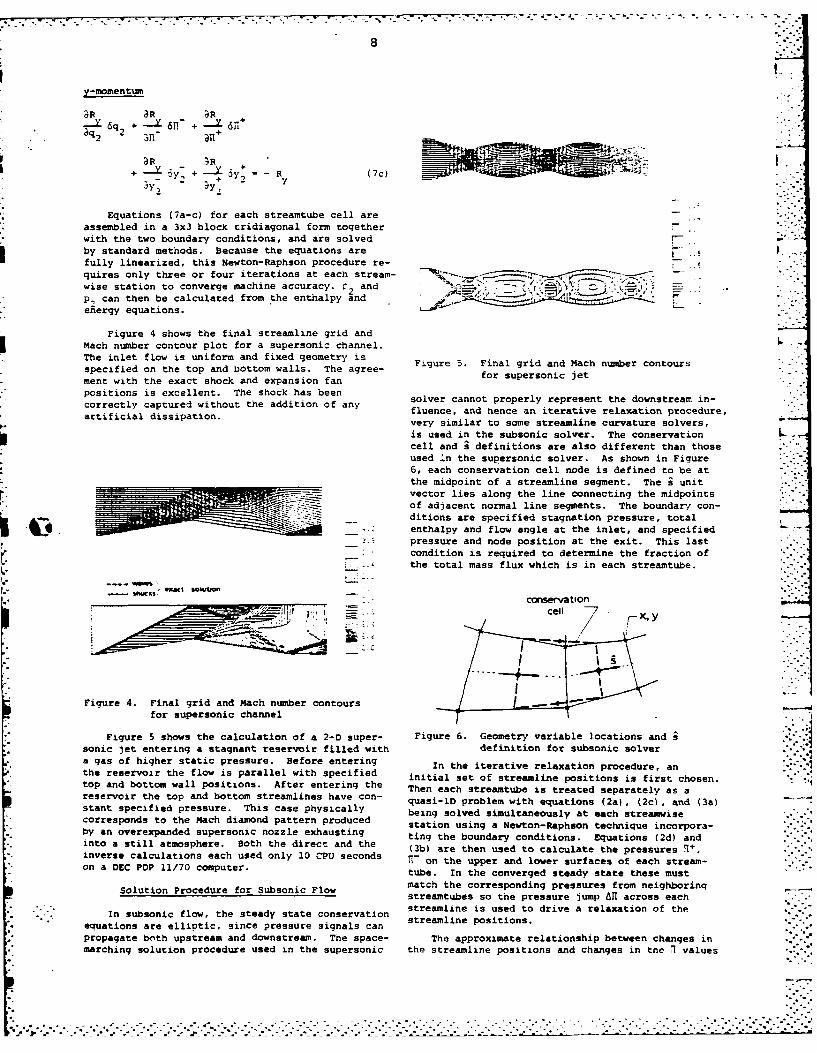
Figure 4 shows the final streamline grid andMach number contour plot for a supersonic channel.The inlet flow is uniform and fixed geometry is Figure 5. Final grid and Mach number contoursspecified on the top and bottom walls. The agree- for supersonic jetment with the exact shock and expansion fanpositions is excellent. The shock has beencorrectly captured without the addition of any solver cannot properly represent the downstream in-corecl c pdtion ofluence, and hence an iterative relaxation procedure,artificial dissipation. very s-imilar to some streamline curvature solvers,
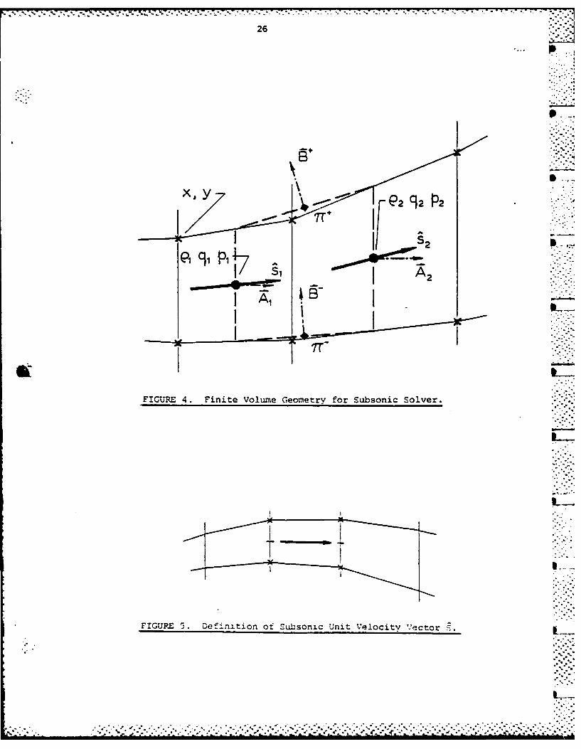
is used in the subsonic solver. The conservation L7cell and i definitions are also different than those
used .n the supersonic solver. As shown in Figure6, each conservation cell node is defined to be atthe midpoint of a streamline segment. The i unitvector lies along the line connecting the midpointsof adjacent normal line segments. The boundary con-S ditions are specified stagnation pressure, total
, " enthalpy and flow angle at the inlet, and specifiedpressure and node position at the exit. This lastcondition is required to determine the fraction of
-- the total mass flux which is in each streamtube.
.2act bOttof
_ _ _ _ _.-__ _conservation
__, " .
Figure 4. Final grid and Mach number contoursfor supersonic channel
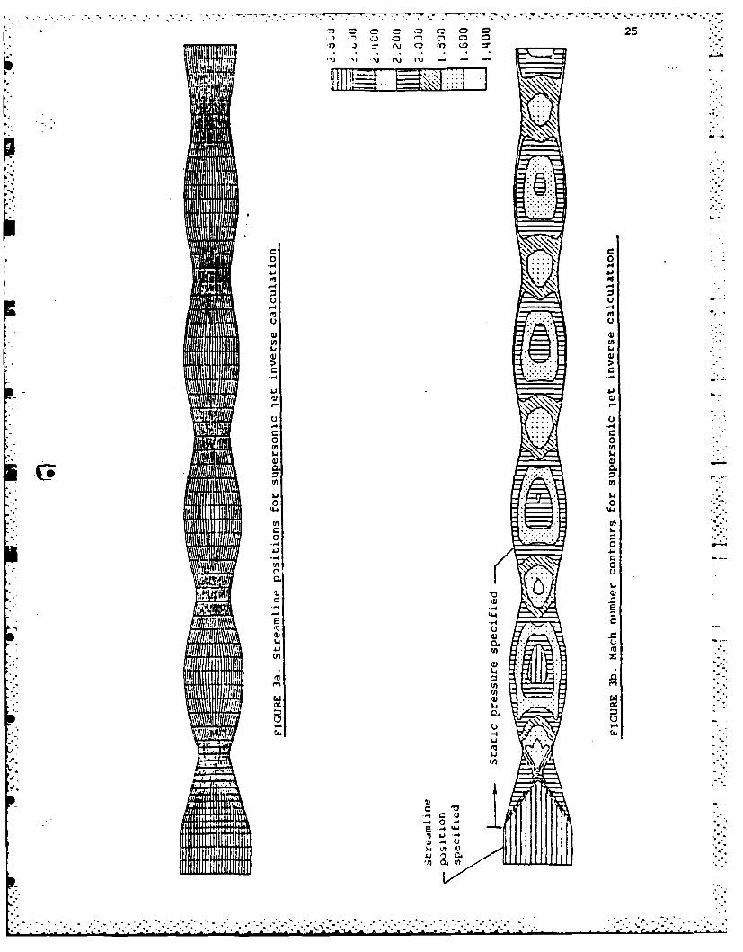
Figure 5 shows the calculation of a 2-D super- Figure 6. Geometry variable locations and -sonic jet entering a stagnant reservoir filled with definition for subsonic solvera gas of higher static pressure. Before entering n i vo cu?, " In the iterative relaxation procedure, an ,'-the reservoir the flow is parallel with specified initial set of streamline positions is first chosen.top and bottom wall positions. After entering the Then each streamtube is treated separately as areservoir the top and bottom streamlines have con- quasi-lD problem with equations (2a) , (2c) , and (3a)stant specified pressure. This case physically being solved simultaneously at each streamwisecorresponds to the Mach diamond pattern produced station using a Nevton-Raphson technique incorpora-by an overexpanded supersonic nozzle exhausting ting the boundary conditions. Equations (2d) andinto a still atmosphere. Both the direct and the (3b) are then used to calculate the pressures n*",inverse calculations each used only 10 CPU seconds t- on the upper and lower surfaces of each stream-
*. on a DEC PDP 11/70 computer. tube. In the converged steady state these must
Solution Procedure for Subsonic Flow match the corresponding pressures from neighborinqstreamtubes so the pressure jump An across eachstreamline is used to drive a relaxation of the
1 ". In subsonic flow, the steady state conservation streamline positions.equations are elliptic, since pressure signals can
. propagate both upstream and downstream. The space- The approximate relationship between changes in* marching solution procedure used in the supersonic the streamline positions and changes in the 1 values
l "
is obtained from the linearized isentropic pressure- __
area relation and the pressure-curvature relation.
2
1 A 2 A 1 P2 A 2 2B-b1-M 1-M2
-fl- _ q 2 - _ypM2 c (9)
In these equations , are the small changesin pressure, cross-sectional area, streamlinepressure and curvature, and M is the local Machnumber. After substituting the dependence of A andK on the changes in coordinate positions? we find I I 'IIthe equation for the j required to eliminate the Ipressure mismatch AR across the streamlines to be, ....
2 2 22 2) A an.,.- M + usdn) - iM (10)1 .Y .p 2 .. 3 s
U and 2 are difference operators defined by C-0s s
2 .. . Figure 7a. Final grid and Mach number contourssi 0 i-l,j +2jij +ii+l,j ) / 4 (11) for subsonic bump
F2 ...
*sii,j = (Yi-l,j - 2Yi, +y i+ l j
)/As (12) 0.003C
0. 002E
and e2 are similarly defined operators in the 0.002normal direction. Equation (10) is similar to the 0.0018streamline curvature relaxation method used byKeith et al [2), e pd the iterative equation in the .::.. . . . .... 0.00.4
solution of the potential equation (5]. The 0.0010boundary conditions required for equation (10) arey-0 on the walls and at the exit, and 6ni0 at the 0.0006
inlet. The latter corresponds to a fixed inlet : ::.2 .:-: . . x:v..0.0002flow angle. Equation (10) is solved using a .. . . -0.0002
standard SLOR technique, the streamline positions .......
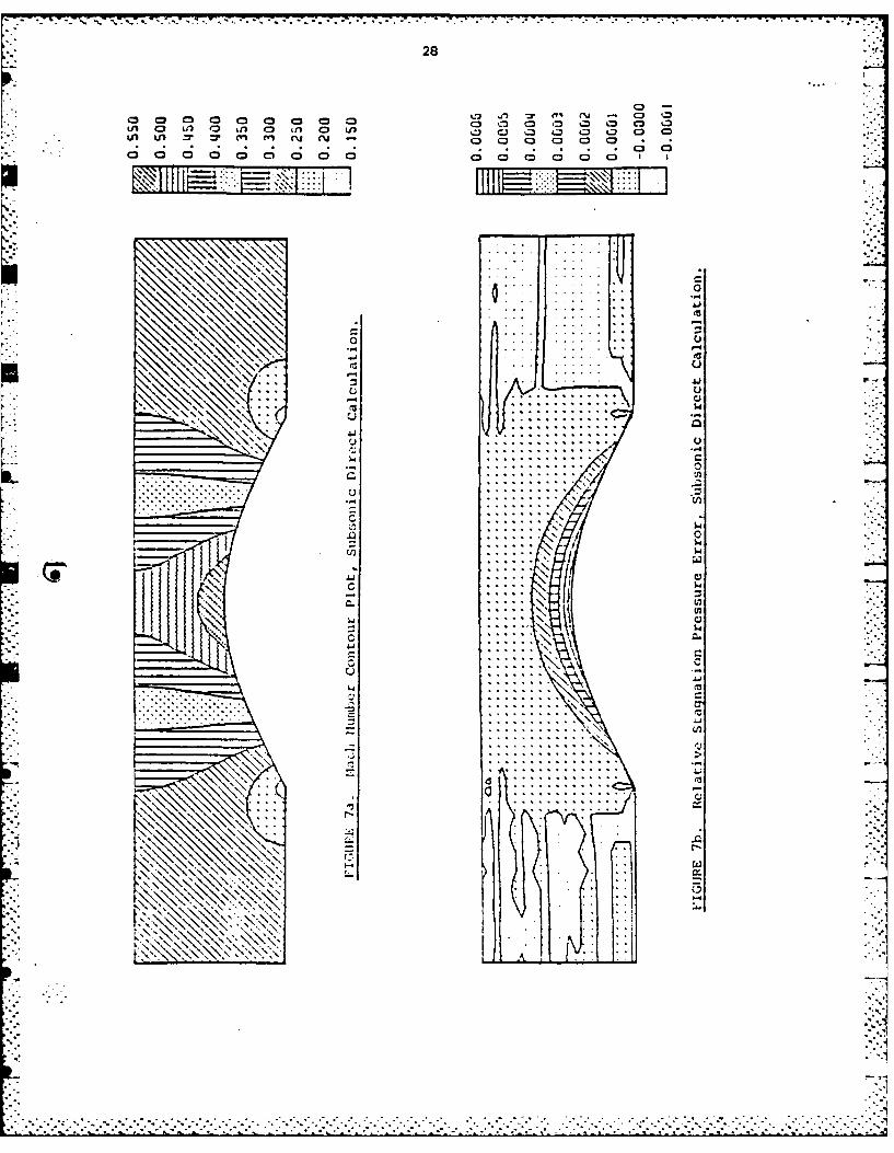
are updated with y, and the cycle repeated until y ...- C.000and AH become acceptably small. This SLOR relax-ation technique limits the overall spectral radius Figure 7b. Relative stagnation pressure loss forof the scheme to l-O(Ax 2 ,Ay 2 ). subsonic
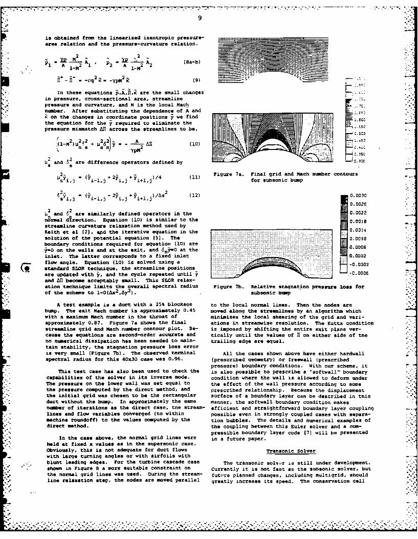
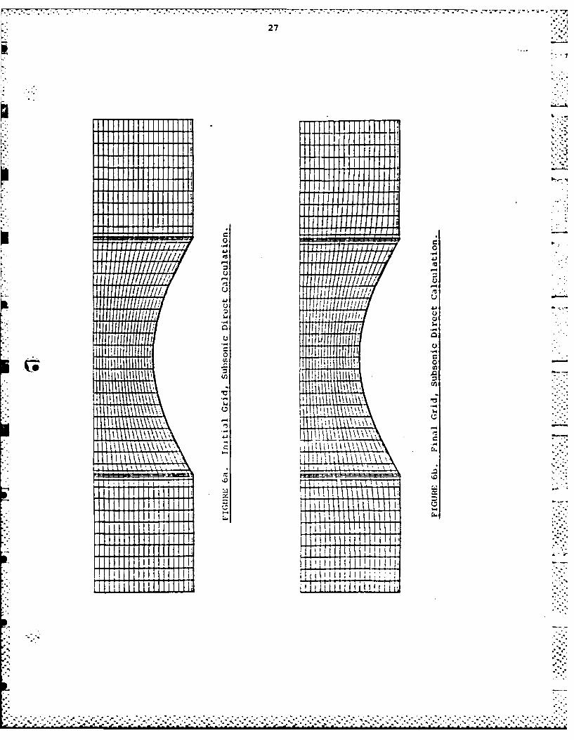
A test example is a duct with a 25% blockage to the local normal lines. Then the nodes arebump. The exit Mach number is approximately 0.45 moved along the streamlines by an algorithm whichwith a maximum Mach number in the throat of minimizes the local shearing of the grid and vari-approximately 0.87. Figure 7a shows the final ations in streamwise resolution. The Kutta conditionstreamline grid and Mach number contour plot. Be- is imposed by shifting the entire exit plane ver-cause the equations are second-order accurate and tically until the values of R on either side of theno numerical dissipation has been needed to main- trailing edge are equal.tain stability, the stagnation pressure loss erroris very small (Figure 7b). The observed terminal All the cases shown above have either hardwallspectral radius for this 40x30 case was 0.96. (prescribed geometry) or freewall (prescribed
pressure) boundary conditions. With our scheme, itThis test case has also been used to check the is also possible to prescribe a "softwall" boundary
capabilities of the solver in its inverse mode. condition where the wall is allowed to deform underThe pressure on the lower wall was set equal to the effect of the wall pressure according to somethe pressure computed by the direct method, and prescribed relationship. Because the displacementthe initial grid was chosen to be the rectangular surface of a boundary layer can be described in thisduct without the bump. In approximately the same manner, the softwall boundary condition makesnumber of iterations as the direct case, the stream- efficient and straightforward boundary layer couplinglines and flow variables converged (to within possible even in strongly coupled cases with separa-machine roundoff) to the values computed by the tion bubbles. The details and numerical examples ofdirect method. the coupling between this Euler solver and a com-
pressible boundary layer code (71 will be presentedIn the case above, the normal grid lines were in a future paper.
held at fixed x values as in the supersonic case.Obviously, this is not adequate for duct flows Transonic Solver
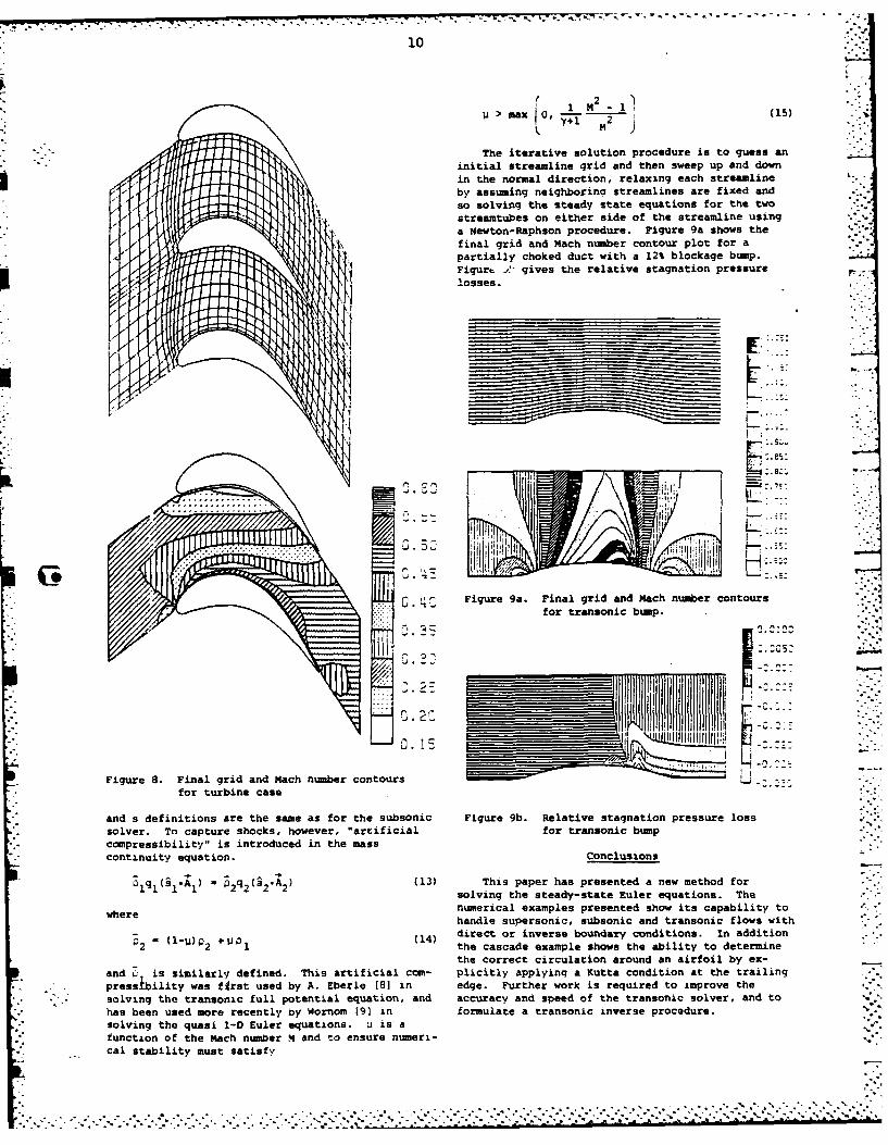
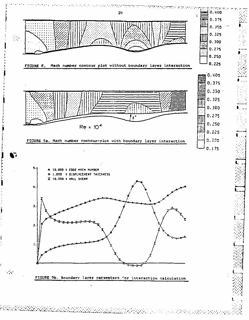
- with large turning angles or with airfoils withblunt leading edges. For the turbine cascade case The transonic solv-r is still under development.shown in Figure 8 a more suitable constraint on Currently it is not fast as the subsonic solver, butthe normal grid lines was used. During the stream- futtvre planned changes, including multigrid, shouldline relaxation step, the nodes are moved parallel greatly increase its speed. The conservation cell
....................................... . . . . . . . . . .
. .. . . . . . . . . . . . . . . . . . . . .• o- •. - . . . . . . . ....- •o-.-° . . . . . - .- . . - - . oo . . . o . .
10
S M2 *"2Si 71 -i1 (15).:aIU A(~y 1 2 1i > max 0, Y + M2 J.(5
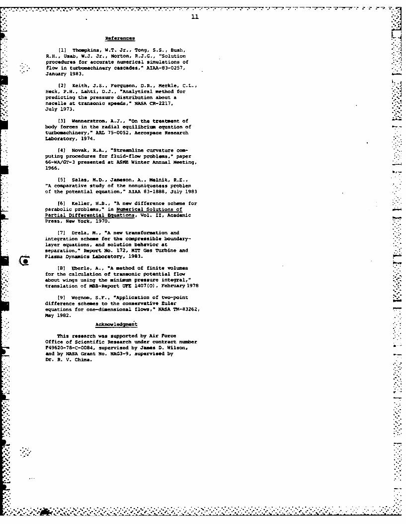
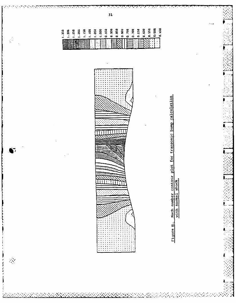
The iterative solution procedure is to guess aninitial streamline grid and then sweep up and downin the normal direction, relaxing each streamlineby assuming neighborino streamlines are fixed andso solving the steady state equations for the twostreamtubes on either side of the streamline usinga Newton-Raphson procedure. Figure 9a shows thefinal grid and Mach nmber contour plot for apartially choked duct with a 12% blockage bump.FigurL .'- gives the relative stagnation pressurelosses.
, --.- .. "
C..
Q Figure 9a. Final grid and Mach number contoursfor transonic bump.:
II t" ,n,
._______________ _ . -"
Figure S. Final grid and Mach number contoursfor turbine case
and s definitions are the same as for the subsonic Figure 9b. Relative stagnation pressure losssolver. To capture shocks, however, "artificial for transonic bumpcompressibility" is introduced in the masscontinuity equation. Conclusions
-lql I* A 2q2( 2.A 2) (13) This paper has presented a new method forsolving the steady-state Euler equations. The
where numerical examples presented show its capability tohandle supersonic, subsonic and transonic flows with
Cl(I-u) 2 + (14) direct or inverse boundary conditions. In additionthe cascade example shows the ability to determinethe correct circulation around an airfoil by ex-
and . is similarly defined. This artificial cam- plicitly applying a Kutta condition at the trailingpressibility was first used by A. Eberle [8) in edge. Further work is required to improve thesolving the transonic full potential equation, and accuracy and speed of the transonic solver, and tohas been used more recently by Wornom 19] in formulate a transonic inverse procedure.solving the quasi 1-D Euler equations. u is a
function of the Mach number M and to ensure numeri-cal stability must satisfy
-7'S.
... . . . . . . . ................""'.'..,"."...."...-.""- . , " - ,""""• , :" "2"" " " - - _'2"-";2Z2.. 2'I
.: ~11.'.
References
(11 Thompkins, W.T. Jr., Tong, S.S., Bush,R.H., Usab, W.J. Jr., Norton, R.J.G., "Solutionprocedures for accurate numerical simulations offlow in turbomachinery cascades," AIAA-83-0257,January 1983.
(2] Keith, J.S., Ferguson, D.R., Merkle, C.L.,Heck, P.H., Lahti, D.J., "Analytical method forpredicting the pressure distribution about anacelle at transonic speeds," NASA CR-2217,July 1973.
[3] Wennerstrom, A.J., "On the treatment ofbody forces in the radial equilibrium equation ofturbomachinery," ARL 75-0052, Aerospace ResearchLaboratory, 1974.
[4) Novak, R.A., "Stremline curvature com-puting procedures for fluid-flow problems," paper66-WA/GT-3 presented at ASNE Winter Annual Meeting,1966.
[5] Salas, M.D., Jameson, A., Melnik, R.E.,"A comparative study of the nonuniqueness problemof the potential equation," AIAA 83-1888, July 1983
[61 Keller, H.B., "A new difference scheme forparabolic problems," in Numerical Solutions ofPartial Differential Equations, Vol. II, AcademicPress, New York, 1970.
(7] Drela, M., "A new transformation andintegration scheme for the compressible boundary-layer equations, and solution behavior atseparation," Report No. 172, MIT Gas Turbine andPlasma Dynamics Laboratory, 1983.
[8) Eberle, A., "A method of finite volumesfor the calculation of transonic potential flowabout wings using the minimum pressure integral,"translation of MB-Report UFE 1407 (0), February 1978
[9] Wornom, S.F., "Application of two-pointdifference schemes to the conservative Eulerequations for one-dimensional flows," NASA TM-83262,May 1982.
Acknowledgment
This research was supported by Air ForceOffice of Scientific Research under contract numberF49620-78-C-0084, supervised by James D. Wilson,and by NASA Grant No. NAG3-9, supervised byDr. R. V. Chima.
-. -. -" ~ ~ ~ - 77 77~~ 7. P_ W-s . . - . . . . .
N 12
APPENDIX 2
CONSERVATIVE STREAMTUBE SOLUTIONOF STEADY-STATE EULER EQUATIONS
by
M. DrelaM. Giles
CFDL-TR-83-6 November 1983
This work was supported by NASA TrainingGrant NGT22-009-901 and the Air ForceOffice of Scientific Research undercontract number F49620-78-C-0O84, super-vised by James D. Wilson.
Department of Aeronautics and AstronauticsMassachusetts Institute of Technolocy
Cambridge, Massachusetts 02139j
13
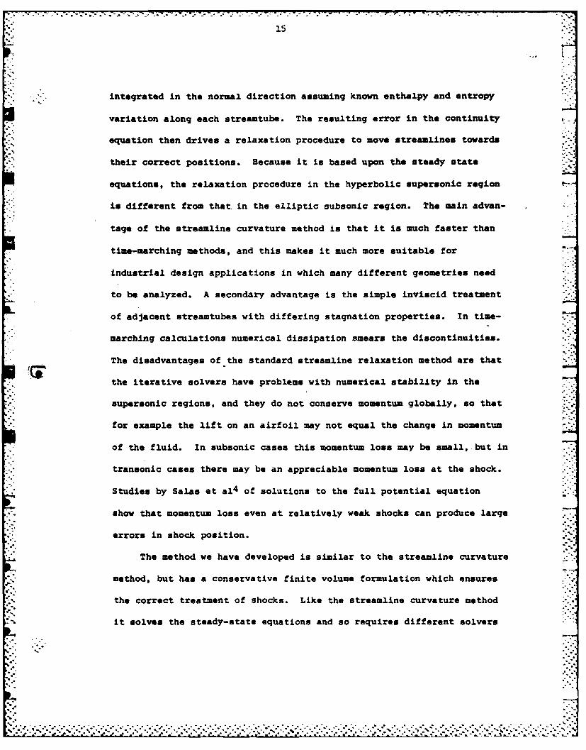
Abstract
This report presents preliminary results obtained using a new
method for solving the steady state Euler equations. The method is
similar to streamline curvature methods but has a conservative finite
difference formulation which ensures correct shock capturing. In
supersonic applications the solution is obtained by space-marching while
in subsonic applications an iterative elliptic relaxation procedure,
similar to potential methods, is used. Numerical results are given for;
a) Supersonic jet entering still reservoir (Inverse calculation)
b) Subsonic Ni's bump with 40% blockage (Direct and inverse)
c) Subsonic bump with boundary layer coupling to calculate a separation
bubble
Li d) Transonic Ni's bump with 10% blockage (Direct calculation)
. . ..- .
- .. . . -
.~~~~~~~~~~~~~~~~~~.... .o. • . . - ...... °.. ..... ,.... ' ''" ... "°........... ." .. °° ."o°o
14
....
: -':';- I )Introduction :
At present most methods for the numerical calculation ofstay
state transonic solutions of the Euler equations are based upon a
conservative finite volume approximation to the unsteady equations of
motion2. This approach has two good features. The first is that it
is conceptually straightforward since the unsteady equations are
hyperbolic in time and so the same numerical procedure can be used in
both the subsonic and supersonic regions. The second is that the
conservative finite volume formulation guarantees the correct Rankine-
Hugoniot shock jump relations regardless of the details of the shock
calculation. The principal disadvantage is that the convergence rate is
limited by the relatively slow propagation of wavelike disturbances
throughout the domain and their reflection at the boundaries of the
computational domain. Current methods try to overcome this limitation
by a variety of acceleration methods such as variable time steps,
implicit operators with larger time steps, and multigrid with larger
time steps on coarser grids, but computation times remain an
order-of-magnitude larger than for the solution of the steady-state
transonic full potential equation, using iterative relaxation methods,
enhanced by multigrid.
An older approach is the Streamline Curvature method which is an
iterative relaxation procedure which solves the equations of motion in
intrinsic coordinates1 ,5 ,6 . In one version an initial set of
streamlines is guessed, the steady-state normal momentum equation is
.................................................... .. ..• ... . . . .. . . . -
15
integrated in the normal direction assuming known enthalpy and entropy
variation along each streamtube. The resulting error in the continuity
equation then drive. a relaxation procedure to move streamlines towards
their correct positions. Because it is based upon the steady state
equations, the relaxation procedure in the hyperbolic supersonic region 0-7
is different from that in the elliptic subsonic region. The main advan-
tage of the streamline curvature method is that it is much faster than
time-marching methods, and this makes it much more suitable for
industrial design applications in which many different geometries need
to be analyzed. A secondary advantage is the simple inviscid treatment
of adjacent streamtubes with differing stagnation properties. In time-
marching calculations numerical dissipation smears the discontinuities.
The disadvantages of the standard streamline relaxation method are that
the iterative solvers have problems with numerical stability in the
supersonic regions, and they do not conserve momentum globally, so that
for example the lift on an airfoil may not equal the change in momentum
of the fluid. In subsonic cases this momentum loss may be small, but in
transonic cases there may be an appreciable momentum loss at the shock.
Studies by Salas et a14 of solutions to the full potential equation
show that momentum loss even at relatively weak shocks can produce large
errors in shock position.
The method we have developed is similar to the streamline curvature
method, but has a conservative finite volume formulation which ensures
the correct treatment of shocks. Like the streamline curvature method
it solves the steady-state equations and so requires different solvers
1. 1.-, -% "4-* . . . - * . * * * * - - - * .*.
16
or solution algorithms, for purely supersonic, purely subsonic, or
transonic problems. The supersonic solver marches in streamwise steps
downstream from a known inlet flow. The subsonic solver starts from a
guessed set of streamline positions, solves each streamtube problem as a
separate quasi 1-D problem, and then relaxes all the streamline
positions to satisfy pressure continuity across streamlines. The tran- ".
sonic solver is similar to the subsonic solver but requires numerical
dissipation in the supersonic region, and relaxes one streamline at a
time instead of all simultaneously. At the present time the supersonic
and subsonic solvers are both robust and very fast, but the transonic
solver requires further improvement.
2) Sipersonic Solver
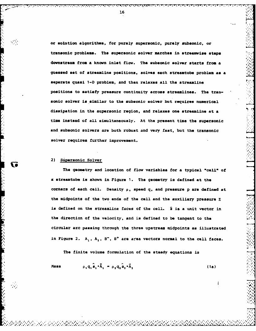
The geometry and location of flow variables for a typical "cell" of
a streamtube is shown in Figure 1. The geometry is defined at the
corners of each cell. Density p, speed q, and pressure p are defined at
the midpoints of the two ends of the cell and the auxiliary pressure R"
is defined on the streamline faces of the cell. ^ is a unit vector in
the direction of the velocity, and is defined to be tangent to the
circular arc passing through the three upstream midpoints as illustrated
*in Figure 2. Al, A, B-, B+ are area vectors normal to the cell faces.
The finite volume formulation of the steady equations is
Mass pjq s =*A1 -P 2 q 2 s 2*
2 (la)
-.. " . . . . .. * . . . . . . . . * .,- . " . P ~ . .
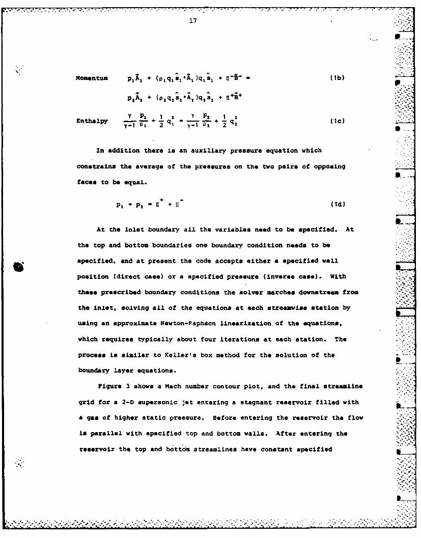
17
p.-
Momentum pill + (p 1 qls1*X1 )ql;l + '" " (1b)
*..-.-. -.
pA 2 + (P2q2s2 A2 )q2 2 , .- '
Y P, 1 Y P2 2
Enthalpy - Pi + q - -52 + q2 (1c)
In addition there is an auxiliary pressure equation which
constrains the average of the pressures on the two pairs of opposing
faces to be equal.
PI + P 2 +n (1d)
At the inlet boundary all the variables need to be specified. At
the top and bottom boundaries one boundary condition needs to be
specified, and at present the code accepts either a specified wall
position (direct case) or a specified pressure (inverse case). With
these prescribed boundary conditions the solver marches downstream from
the inlet, solving all of the equations at each streamwise station by
using an approximate Newton-Raphsen linearization of the equations,
which requires typically about four iterations at each station. The
process is similar to Keller's box method for the solution of the
boundary layer equations.
Figure 3 shows a Mach number contour plot, and the final streamline
grid for a 2-D supersonic jet entering a stagnant reservoir filled with
a gas of higher static pressure. Before entering the reservoir the flow
is parallel with specified top and bottom walls. After entering the
reservoir the top and bottom streamlines have constant specified
*'. , . - .':........: -............. 7
18
pressure. This case physically corresponds to the Mach diamond pattern
produced by a supersonic nozzle exhausting into a still atmosphere and
took only 10a on a PDP11/70 to achieve convergence to machine roundoff.
3) Subsonic Solver
Initially our subsonic solver used the same geometry and location
of flow variables as the supersonic solver. Unfortunately there were
problems with numerical stability and unacceptably high errors. These
problems were overcome by going to the slightly different geometry shown
in Figure 4, without needing to resort to numerical dissipation. ThereL
are now two grid structures, a relaxation grid with coordinates defined
at its nodes, and a conservation grid with its corner nodes defined to
be the midpoint of the corresponding streamline faces on the relaxation
.grid. The s unit vector in the direction of the velocity is defined
to be parallel to a line connecting midpoint of normal faces on the
relaxation grid as shown in Figure 5. The steady state conservation
equations are exactly the same as for the supersonic solver but the
solution procedure is totally different. Since the equations are
elliptic, an iterative relaxation procedure, very similar to some
streautube curvature solvers, is required. First an initial set of
streamline positions is chosen. Then each streamtube is treated
separately and Equations (la-ld) are solved simultaneously at each
streamwise station using a Newton-Raphson technique incorporating the
boundary conditions, specified stagnation pressure total enthalpy and
exit pressure. These calculations produce pressures H+ , n- on the-L
• .---------------------------------
19
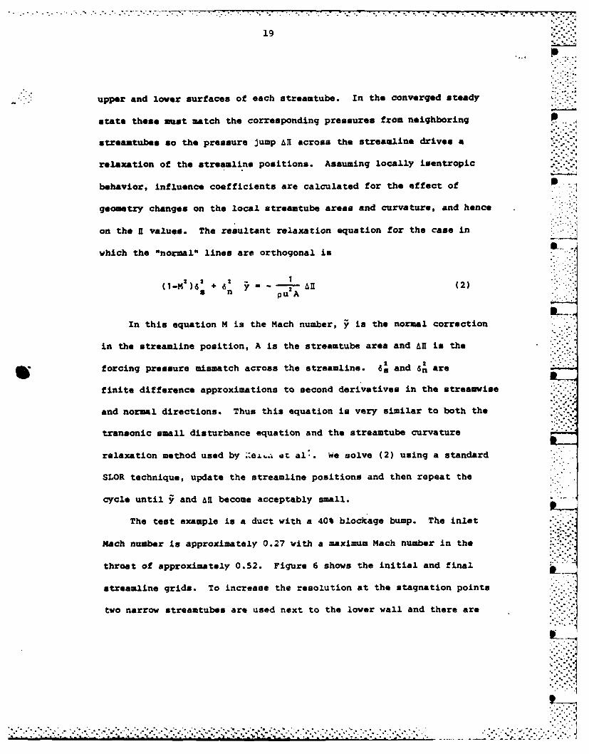
- ~..*upper and lower surfaces of each streautube. In the converged steady
state these must match the corresponding pressures from neighboring
streantubes so the pressure jump anl across the streamline drives a --
relaxation of the streamline positions. Assuming locally isentropic
behavior, influence coefficients are calculated for the effect of
geometry changes on the local streamtube areas and curvature, and hence
on the RI values. The resultant relaxation equation for the case in
which the "normal" lines are orthogonal is
(1-M,2 a + 61j.----Al (2)s n Y puA a
In this equation M is the Mach number, is the normal correction
in the streamline position, A is the streamtube area and anl is the
2 2
forcing pressure mismatch across the streamline. as and an are
finite difference approximations to second derivatives in the streamvise
and normal directions. Thus this equation is very similar to both the
transonic small disturbance equation and the streamtube curvature
relaxation method used by at~ al:. we solve (2) using a standard
SLOR technique, update the streamline positions and then repeat the
cycle until ~;and anl become acceptably small.
The test example is a duct with a 40% blockage bump. The inlet
Mach number is approximately 0.27 with a maximum Mach number in the
throat of approximately 0.52. Figure 6 shows the initial and final
streamline grids. To increase the resolution at the stagnation points
two narrow streamtubes are used next to the lover wall and there are
• -" -."-".- -'"."." " .:;' .' -.: "-":. :-' .7 --.-""•.-" "" -.."""' ,T: -"". .."." ." ," ..-."-- .- . * 1-- ..' .
7-7. T. -
20
additional normal lines at the front and back of the bump. The only
discernable difference between the initial and final grid is a
thickening of the streastubes near the stagnation point. Contour plots
of the Mach number and relative stagnation pressure loss are shown in
Figure 7. Because the equations are second-order accurate and no
numerical dissipation has been needed to maintain stability, the
stagnation pressure loss is much lower than for time-marching codes2 .
This test case has also been used to check the capabilities of the
solver in its inverse mode. The pressure on the lower wall was set
equal to the pressure computed by the direct method, and the initial
grid was chosen to be the rectangular duct without the bump. In approx-
imately 50 iterations the streamlines and flow variables converged (to
within machine roundoff) to the values computed by the direct method.
The ability to prescribe wall position and/or wall pressure in our
formulation makes efficient boundary layer (BL) coupling possible even
in strongly coupled cases with separation bubbles (Figures 8, 9a,b).
For this example, a finite difference BL code using a Shifted Box
Scheme8 was used. Simultaneous BL calculations and downstream relax-
ation sweeps are used to drive the Euler and BL edge velocities together
at the displacement surface. During the relaxation of the inviscid
flow, a hybrid boundary condition prescribing a linear combination of
edge pressure and position simultaneously drives these quantities
towards the matching condition. The behavior of the BL is locally
modeled by a u. - s" influence coefficient which is a byproduct of the
BL calculation.- U a -. . S. ,
21
The coupled solution in Figures 9a,b required 120 relaxation sweeps
and 12 BL calculations to fully converge. The purely inviscid case in
Figure 8 required 50 relaxation sweeps. This preliminary coupling case
indicates that coupled calculations will not require drastically more
computation time than purely inviscid calculations.
4) Transonic Solver
The transonic solver is still under development. The current
solver is not very fast or robust but is sufficient to demonstrate the
feasibility of this approach for transonic cases. The grid geometry is
the same as the supersonic solver. At supersonic points the supersonic
a definition is used. At subsonic points is defined to be tangent
to the circle passing through the neighboring midpoints as shown in
Figure 1. The main feature of the transonic steady state equations is
the introduction of an "artificial compressibility" term in the
continuity equation. The mass conservation equation is
- .%;1q1 (s1 A1 ) - 2q 2 (s2 A 2
where
- l-Pj2 + P1 -
and p, is similarly defined.
This artificial compressibility was first used by A. Eberle7 in
solving the transonic full potential equation, and has been used more
recently by Wornom [31 in solving the quasi I-D Euler equations. i is
., . .. *.*.%*q*., .-- .°*.. - - - - - - - - -
* - . .. .°.
22
a function of the Mach number M and to ensure numerical stability must
satisfy
M -1>i max 0 ,-- -
+1 ,2
The iterative solution procedure is to guess an initial streamline
grid and then sweep from side to side in the normal.direction, relaxing
each streamline by assuming neighboring streamlines are fixed and so
solving the steady state equations for the two streamtubes on either
side of the streamline using a Newton-Raphson procedure.
Figure 10 shows the final grid and Mach number contour plot for a
fully choked duct with a 25% blockage bump.
67.:':.:
23
REFERENCES
1. Keith, J.S.. Ferguson, D.R., Merkle, C.L., Heck, P.H., Lahti, D.J.,
"Analytical method for predicting the pressure distribution about
a nacelle at transonic speeds," NASA CR-2217, July 1973.
2. Thompkins, W.T. Jr., Tong, S.S., Bush, R.H., Usab, W.J. Jr., Norton,
R.J.G., "Solution procedures for accurate numerical simulations of
flow in turbomachinery cascades,"AIAA-83-0257, January 1983.
3. Wornom, S.F., "Application of two-point difference schemes to the
conservative Euler equations for one-dimensional flows," NASATM-83262, May 1982.
4. Salas, M.D., Jameson, A., Melnik, R.E., "A comparative study ofthe nonuniqueness problem of the potential equation," AIAA 83-1888,July 1983. %
5. Wenneratrom, A.J., "On the treatment of body forces in the radialequilibrium equation of turbomachinery," ARL 75-0052, AerospaceResearch Laboratory, 1974.
6. Novak, R.A., "Streamline curvature computing procedures for fluid-
flow problems," paper 66-WA/GT-3 presented at ASME Winter AnnualMeeting, 1966.
7. Eberle, A., "A method of finite volumes for the calculation oftransonic potential flow about wings using the minimum pressure
integral," translation of MBB-Report UFE 1407(0), Feburary 1978.
8. Drela, M., "A new transformation and integration scheme for thecompressible boundary-layer equations, and solution behavior atseparation," Renort No. '2. mIT -as Turbine and Plasma DynamicsLaboratory, 1983.
-. ~ ~ ~ ~ ~ ~ K .. ' ' .-.- <.-.
24
57
7T 2 2P
FIGURE 1.. Finite volume Geometry for Supersonic Solver.
F'IGURE 2. Definition of Suo~ersanic Unit Velocitv Vector S
o n C: 0m 25* 7' '3 C: 0 0 (D~ :
lip,\J CI V r~ ~ - - --
Q-4
040
41.
'U('. fu
Ow 0f
26
A
S2S
I 91 Ti
S1:A=Now~
FICURE 4. Finite Volume Geometry for Subsonic Solver.
---------
FIGURE 5. Definition of Subsonic Unit Velocity Vector I
27
I.II II I II I-
fl PiH
P4 I
"U II / W111 i
1111,01 1111 Hil/jHM ;lit)
I )
11H,,
28
Lml 03 (fl 0'. 4= 0 n 0v C0C 3 C3 c%n Lnf CUJ U - 00 C 0 03 0 03K3 C3l 0i 0 Cf L* C C;J 0 C C C ;
UU
~~1.
2S)
HI 0.30
71 .7;..0.2750.250
FtGURE 8. Mach number contour plot without boundary layer interaction 0.22S
K ~ 0.400
/0.375
_________ o 325
'.*.*.*.- 0.300 I -
0.275
Re: 104 0.250
*FrGUR 9a. Mach number contour-plot with boundary layer interaction 0 ; £~0 I
0. 175
LA 10.000 x EOGE MACH NUMBER0 1.000 1 OISPLACEMENT YN1CiKNES
I. Z 10.000 X WALL SHEAR -
3.
FIUE9btondr aver aram'eters 'or interaction calculation :*>. >*.-
30
FIGURE 1.0. Unit Velocity Vector Definition in Subsonic Regions ofTransonic Calculati~on.
31
, 0 U~0 eI 0 en 08 l 0 0 o ena 0 U
12 a0 a, 10 a, a 0e
. .. . ~ ~. . . .. .. ., , .. .:--- -
Y'IIh I Iii:.1 IIUN II~ii m iii I
0 .
1 Q
.0
.S.. . . . U
"I.I2
.
.. ....-.. ... . . . . . . ."""""'"""" -" ". ":-.1.-1:.:..:.::. .......... ,0_ _.
5' .. . "
• . . . . . . . , ° . , °
.* . . .* *2-"
32
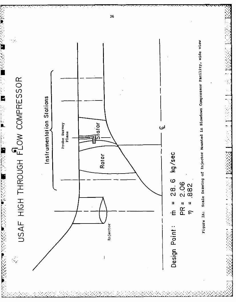
TASK IB: LOSS MECHANISMS AND LOSS MIGRATION IN TRANSONIC COMPRESSORS
Introduction
The objective of this study is to quantify the understanding of loss
production versus loss migration by detailed time-resolved radial
streamline/pathline measurements in the AFAPL High Through Flow
Compressor, a transonic compressor stage, in the MIT Blowdown Compressor.
Streamline tracing in a transonic, unsteady compressor flow requires
that streamlines or pathlines be identified in the presence of
simultaneous first order nonperiodic changes in total pressure and
temperature.
The basic technique is to inject a thin ring of the tracer gas upstream
of the compressor rotor and then survey with a concentration probe at the
rotor exit to map the radial transport of the tracer gas. The injection
ring is then moved radially and the experiment repeated. In this manner
the time-dependent radial transport within a transonic compressor rotor can
be mapped simultaneously with a timeresolved measurement of rotor loss
(from a cotemperal and pressure measurement).
The dual wire aspirating probe will be used for the simultaneous
measurement of time-resolved concentration, temperature, and pressure
possible at frequencies up to 20 KHz. The probe consists of two constant
temperature hot wires operated at different overheat ratios in a channel
with a choked exit. Thus the flow past the wires is at constant Mach
number. The heat flux (and thus the electrical signal) from the wires is a L
function only of freestream total pressure and temperature and gas composi-
%.. -tion. Previously, the probe was used in a flow of constant composition. ..
..-> >-.
%I ,"o ".
33
Thus, the signals from the two wires were sufficient to permit calculation
of the two unknowns, total pressure and temperature. A piggyback total
pressure sensor was used as a redundant check. In this investigation, the
pressure sensor is used to provide the third signal to allow the three
independent variables (concentration, temperature, and pressure) to be
derived at each instant in time.
Progress to Date
Work to date has concentrated on tracer gas selection, probe
calibration, and injector design. The selection of the proper tracer gas
is important. Ideally, the tracer should have the same density as the
main flow while differing in those fluid properties important to the
probe operation: thermal conductivity, viscosity, ratio of specific
heats, and molecular weight. We have examined the suitability of several
gases and gas mixtures in regard to the above criteria and concluded that
the two most promising for use in the Argon-Freon-12 atmosphere of the MIT
Blowdown Compressor are carbon dioxide and Freon 153A. Krypton is also
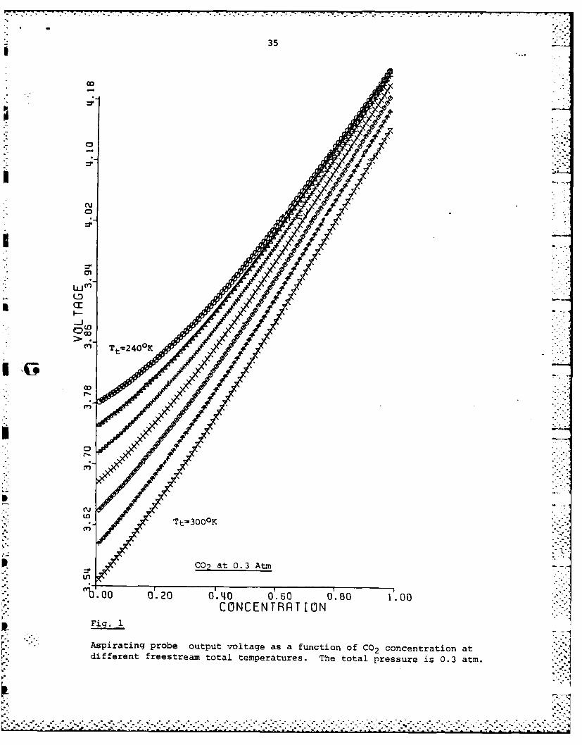
suitable but quite expensive. Figure 1 illustrates the calculated voltage
output from the aspirating probe as a function of gas temperature and
CO2 fractional concentration in the Argon-Freon mixture used in the MIT
Blowdown Compressor Facility.
It is clear from the analysis that the success of the experiment
hinges on the overall stability of the aspirating probe since the variations
due to concentration changes are relatively small, representing the
difference between two large numbers. Preliminary laboratory calibration
tests with CO2 look promising. These tests are continuing, to both
-°___-__ _______. ___. __. o•. .. . . . . . . . . . . . . .o
34
establish the calibration and data reduction procedures and to assess the
long term probe stability.
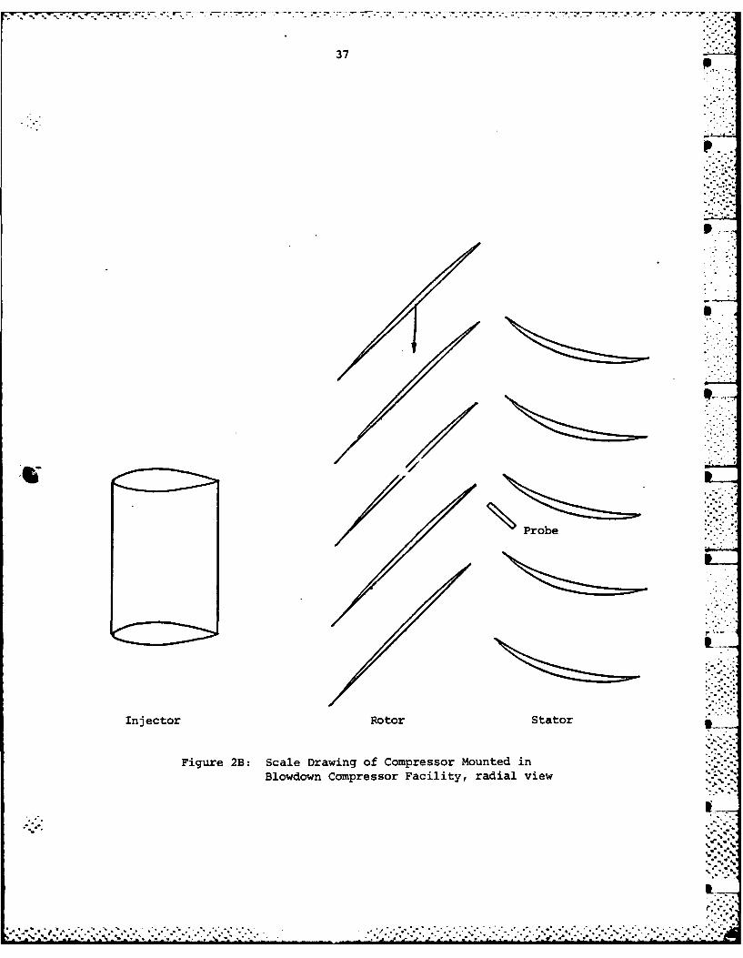
The gas injector has been designed and is now being fabricated. The
design goal is the injection of a 1 - thick sheet of tracer gas with the
same velocity and static pressure as the main flow in order to minimize the
turbulent mixing of this sheet as gas propagates downstream. The injector
(figure 2) consists of a NACA 654-021 airfoil limited to two blade
passages in circumferential extent in order to reduce the amount of
injection gas required. The hollow airfoil contains a plenum (instrumented
with a pressure transducer) feeding a 0.8 mm wide slot at the trailing
edge. The injector is supported by two radial struts of similar
cross-section which carry the injection gas. The entire assembly is
mounted through the tip casing which permits the radial position to be
varied. O-rings provide the seal at this point. The vibrational
frequencies of the injector assembly has been calculated to insure that no
resonances lie within the range that can be forced by the rotor.
An attempt was made to calculate the extent of the radial mixing due
to turbulent shear as the injectant sheet is convected downstream. Because
this is such a strong function of the precise pressure and velocity match
at the injector trailing edge and because various models give such
disparate results, the only believable figures will be those from measure-
ments. These will be done by surveying across the compressor annulus at
the rotor exit station with the blade rows removed, thus establishing a
baseline for comparison with the rotor exit measurements.
It is anticipated that most of the calibration work will be completed
by the time the injector assembly is fabricated. The baseline measurements
described above will then begin.
* *.~ .. * . * * ' * ~ * * * ' * -. ..-
I 35
iC
U
0,
(n
w Tt-34O0K
IL C02 at 0.3 Atm.
Too G'.20 0'.40 0 .60 0'.80 1.00CONCENTART ION
p Fig. 1
r Aspirating probe output voltage as a function Of C02 concentration atdifferent freestream total temperatures. The total pressure is 0.3 atm.
36
44
U
cr-4
0 0
0 W,
544
0
tfl
00
0 0
*(D
00 co
c.4-
U 1.
L. 04(3 H
37
p
Probe
Injector Rotor Stator
Figure 2B: Scale Drawing of Compressor Mounted in. -.
"c..- ..°
Blowdown Compressor Facility, radial view
. .
.: 'Injecor Roor Sttor .
38
TASK II: COMPRESSOR STABILITY ENHANCEMENT USING HUB/CASING TREATMENT
The overall goal of this study is the understanding of the basic
mechanism(s) by which a grooved casing or hub is able to significantly
extend the stable flow range of a turbomachine. A key concept in this is,
in our view, a quantitative appreciation for the fluid mechanics of the
interchange of momentum between the casing and the flow in the endwall
region of the blade passage.
In our first series of experiments, carried out over the past several
years, we showed that a moving grooved hub could have a very potent effect
on stator stall margin and pressure rise [2.1]. (This was the first time
this had been demonstrated.) This result meant that we could examine the
relevant phenomena using the stator passage/moving hub configuration. The
present series of experiments are aimed much more at the basic phenomena
associated with hub and casing treatment, and involve a detailed examina-
tion of the three-dimensional, unsteady flow within the blade passage.
This work will form part of the M.S. Thesis of Mr. Mark Johnson, who is in
the AFRAPT Program.
In previous progress reports, we mentioned the design, development,
and fabrication of the instrumentation and the necessary software to enable
us to examine in detail the unsteady flow in the stator passage. We also
mentioned the design of an optical detector system to interact with our LSI
11/23 microcomputer to monitor the relative position of the grooves
accurately during the experiment. In the 6-month period following that
progress report, we have essentially completed the tasks mentioned above.
In addition, we have also accomplished the following tasks:
.. . . . . . . . . . . . . .. , ... .. . .. .. . .. .. . .. .. . .. .. . .. .. *.
39
(1) With the newly designed and built inlet contraction section mounted
on, measurements of the inlet velocity profile upstream of the single stage
low speed compressor were taken to compare with the previous results as a
check. No substantial difference in the results was observed except
that, as might be expected because of the longer flow path, the boundary
layer on the casing is thicker than before (i.e., with the old inlet
section on).
(2) The compressor characteristics, pressure rise versus flow, were
retaken both for the cases of smooth hub and treated hub to compare with
previous results as a check. This data is shown as Figure 2.1. The large
differences between the smooth wall and the grooved wall pressure rise as
well as stall onset points (essentially at the peaks of the curves) are
evident. Although the relative positions of the curves are close to those
CO measured previously, there is a difference (of about 5%) in the absoluteCO.7
levels of flow and pressure from previous measurement for both smooth wall
and hub treatment. This may be due to the larger inlet boundary layer
resulting in a changed profile presented to the stator. However, because
of the departure of Mr. Johnson for Garrett (where he is working for the
summer, as part of the AFRAPT program) we have not resolved this with any
degree of precision.
(3) Preliminary experiments were carried out to validate and test the
overall data acquisition system. This includes the traverse system for
probe (hot wire or pressure) with three degrees of freedom (linear
translation, angular motion in a radial axial plane in the stator blade
passage, and rotation on its own axis).and the optical detector system, for
................................ . . . .
40
monitoring the groove position.
An inclined hot-wire probe was used to obtain high response data at a
particular point in the blade passage from which the three velocity
components at that point can be reduced. This probe had been separately
calibrated in a GTL jet facility. The spatial resolution achievable with
this current hot wire probe is 2 to 3 Mm.
The data matrix grid can be described by a three-dimensional
co-ordinate system (I,JK) fixed to the laboratory frame. Each I refers to
a plane concentric with the hub surface (for instance I - 1 refers to a
plane 2.25 mm from the hub, I - 2 to that 12.25 m from the hub, etc.).
Each J refers to a plane parallel to a mean-chord plane with J - 1 plane
being closest to the blade auction surface. Finally, each K refers to a
plane parallel to the leading end trailing edge plane with K - 1 plane
being the leading edge plane.
For this set of preliminary experiments, the data matrix chosen is
such that on each I plane (I varies from 1 to 5, I - 5 is roughly the
mid-span plans) there is a 4 by 7 grid (i.e., J - 1 to 4 while K - i to 7).
A separate set of data was taken at grid points outside the above data
matrix grid for ascertaining the periodicity of the flow from passage to
passage. In the preliminary experiments, hot wire data were acquired for
runs with smooth hub wall as well as groove-treated hub wall, with the
compressor operating at 2600 rpm and at flow coefficients varying from 0.24
to 0.37. The hot wire data have not yet been reduced to yield the three-
dimensional flow field in the blade passage region close to the smooth and
treated hub surfaces. However, it does appear from this set of experi-
:'-"""'" " "-"" .. ."- - - ..'-.'. ".'. .-' . -. "- -. .-.- . .....-.. .-... .. . - -. .-".- .-".o. o..-, .-° o .4
41
ments, that the overall data acquisition system performs satisfactorily.
We do not as yet rule out any future modifications and refinements to the
data-acquisition system if we find it necessary to do so.
We hope that, in the next few months, efforts will be expended to
obtain the three-dimensional velocity field in the passage from this hot- -
wire data, and to examine possible three-dimensional presentations of this
information. Such a presentation would enhance our ability to view the
results in a more interpretative and constructive way. This preliminary
set of experiments should also enable us to refine and to plan our
measurements of the flow in the next set of experiments. When this set of - -
measurements has been carried, out, we also hope to take up again our
theoretical (modelling) work on this problem. This is an area which we
have not had time to pursue over the past year but one that is a crucial
part of a balanced research effort on this topic.
Reference
2.1 Cheng, P., Drell, M.E., Greitzer, E.M. and Tan, C.S., "Effects of -Compressor Hub Treatment on Stator Stall and Pressure Rise," J.Aircraft, 21, 469-476. -
-...........
L• Af.• . .o-' . . 5*-o , *~ ~ ~ * f* ~ * - 5 * ** - ** * * ** * ~ . o °
42
* STPTOR STPTIC TO STPTIC PRESSURE RISE
C))
...... ...........
.. ...... ... .. -.. . ..
c0.. .... .... ..... . .... .
.L..u ......... .. .. ......... .... .... .. ......
..........0......... ..... .. ..... .... ..................
0< ....... .............. ......... ... .
0n............... ...... .. ..... . .. ...
0._ _ _ _ __3_ _ _ _ _
oC 5 02D 50 003 .~FLO.... COFIIN ......... ME...
FGueo
43
TASK III: INLET VORTEX FLOW DISTORTIONS IN GAS TURBINE ENGINES
During the past six months, we have nearly completed the experimental
part of our investigations of this phenomenon (at least the first phase -
the vortex formation process). These have provided not only quantitative
information on vortex strength, but also insight into the basic vortex
structure associated with this type of flow. A paper on this work is
currently being prepared for submission. A draft of this paper is
presented below.
% %
-n.
............................................... -. * ...
44
INTRODUCTION
Gas turbine engine operation near the ground in often associated withthe presence of a strong vortex which stretches between the ground and theengine inlet. This "inlet vortex" (or ground vortex) can be of concernbecause of the effects it can have on the engine. These include foreignobject damage, increased blade erosion due to dirt ingestion (1], andcompressor surge [2].
Investigations of the inlet vortex have identified two basic mechanisms .that are responsible for its formation [3]. The first is the amplificationof the vertical component of ambient vorticity, i.e., vorticity created farustream of the inlet, as the vortex lines are convected into the inlet. A-detailed description of this process, including calculations of the driftof these vertical vortex lines in the three-dimensional flow produced by aninlet near a ground plane, is given in [3].
The second mechanism for vortex formation, however, does not depend onthe presence of ambient vorticity. This process can occur in a flow thatis irrotational far upstream, for an inlet in crosswind. In this situation,because of the variation in circulation along the inlet, a trailing vortex(from the rear side of the inlet) is also present. It is this secondmechanism, which appears to be less well understood, that forms the focusof the present paper.
In previous investigations, the flow regimes encountered with aninlet/ground plane configuration were found to depend strongly on twoparameters: 1) the ratio of inlet (average) velocity to upstream velocity,Ui/Ue, and 2) the ratio of inlet centerline height to inlet insidediameter, H/D. For an inlet in crosswind in an upstream irrotational flow,at low values of velocity ratio, Ui/Ue, and/or high values of H/D, twocounter-rotating vortices trailed from the rear of the inlet. These aredepicted in Figure 1(a), which is taken from the hydrogen bubble flowvisualization studies in [3]. When H/D was fixed and the velocity ratiowas increased, or H/D decreased for a fixed velocity ratio, an inletvortex/trailing vortex system was formed, as indicated in Figure 1(b).
As described in [3], the presence of this trailing vortex isassociated with the variation in circulation (i.e., circulation round theinlet) along the axial length of the inlet. A schematic of the location ofthe vortex lines in the flow shown in Figure 1(b), which indicates this, isgiven in Figure 2. The circulation around curve C2 , which is justforward of the inlet lip and encloses the inlet vortex, is r2. Far fromthe lip, around curve C1 , it is argued that the circulation is small. Ifthis is so, there must be a trailing vortex with circulation of strengthapproximately -r 2 , an indicated in the figure. It should be emphasizedthat igure 2 is a very simplified picture, and that we will examine thevorticity field in more detail below.
.. . . . . . . . * ......-- .- * .... ~ * - *. . . . . . . .... *.-.o' *-*.*,
45
The previous investigations, which were carried out in a water tunnel,were only qualitative in nature. In particular, they provided only veryrough estimates of the key fluid mechanic parameters: vortex strength andposition. These are required for the determination of the velocitynon-uniformity presented to the engine or the degree to which particles areingested. The present study was thus undertaken to quantify the observedphenomena; more precisely, to provide quantitative measurements of thethree-dimensional vortex flow. As reported in [4], a facility for makingthese measurements has been designed, built, and calibrated. Some initialmeasurements were also reported, from which the overall structure of theflow field could be inferred, and this was found to agree with theconceptual picture developed from our water tunnel observations.
This paper presents the first detailed measurements of the three-dimensional flow associated with the inlet vortex. There are two mainpoints that are addressed. The first is to show quantitatively that thecirculation of the inlet and trailing vortices are (as hypothesized in [3])essentially equal and opposite. The second is to define the circulationand- the location (inside the inlet) of the inlet vortex for values of thepertinent nondimensional parameters which are representative of thoseoccurring for actual aircraft, since this is a situation of strong practicalinterest. In addition to these points, further information about thevortical structure of these flows, obtained from water tunnel flow visuali-zation, will also be described.
EXPERIMENTAL FACILITY AND EXPERIMENT DESIGN
All of the quantitative measurements reported were conducted in the-M.I.T. Wright Brothers Wind Tunnel. A layout of the tunnel is shown inFigure 3. The tunnel is closed circuit, with an elliptical test section3.05 m wide, 2.3 m high and 4.6 m long. During this investigation a 2.4 mwide ground plane was mounted 0.46 m above the bottom of the test section.The leading edge of this ground plane was rounded and drooped to avoid flowseparation.
The mean velocity in the test section is controlled by either a
variable pitch propeller, which can induce velocities up to 80 m/s, or an
auxiliary fan (a large attic fan), which is suitable for speeds up toroughly 3 m/s. The propeller and fan controls, and the data acquisition
system, are located in a control room adjacent to the test section.Further information is given by Markham [5].
The flow through the inlet was created by a three-stage centrifugalblower located outside the tunnel. This was designed with backward leaningblades so as to obtain as large a stable flow range as possible, in orderto have flexibility in the carrying out of parametric studies. The inletface average velocity, an important parameter of the experiment, wascalculated from the measured pressure drop across a calibrated perforated
7 plate in the inlet blower/duct system. In the experiments, the maximum
* -. *. . *.x.......................................................-
-, -7 -j
46
inlet velocity vas 135 m/s, so that compressibility effects were not 7
" important. Further details of the construction and calibration of theI • . facility for inlet vortex flow measurements are given in (4] and [6].
The inlet model used is a circular cylinder with no centerbody. Theinside diameter was 0.15 m and the outside diameter was 0.2 m. The inletlip was designed to have no separation over the range of conditions ofinterest, using the procedure developed by Stockman and Boles [7],[8],which yielded an inlet lip geometry composed of elliptical segments.
The nomenclature used to describe positions on and inside the inlet isthat the theta (0) coordinate refers to angular position around the inlet.In the crosswind configuration used, the inlet is at ninety degrees to themean flow, 6 " 0 is upstream (at the "leading edge*), 0 - 90 is on the topof the inlet, 6 - 180 is at the rear, and 6 - 270 is at the bottom. Theseconventions apply for measurements on both the inner and outer surface ofthe inlet. The axial coordinate is measured along the inlet axis, with thezero location being at the inlet lip, and the radial coordinate is theradial distance from the axis of the inlet.
Although there is no difficulty in obtaining kinematic similaritybetween the parameters in the model test and in tbe actual situation, thisis not so for dynamic similarity. In particular, the large size of anactual aircraft engine precludes exact Reynolds number scaling forpractical model tests. For this reason, the inlet models were equippedwith 1.5 mm diameter "trip wires", at ± 67 degrees. These preventedlaminar separation or operation in the transition regime betweensubcritical and supercritical operation, where the flow depended strongly
on small surface finish irregularities. When the model was operated withno flow through the inlet, the use of the trip wires produced staticpressure distributions similar to those round a circular cylinder at theactual (full-scale) Reynolds numbers of interest. Description of theconsiderations associated with the use of the trip wires can be found in[4] and [6].
Two models were machined for the experiments, one of plexiglas and theother of aluminum. The former was used for flow visualization, and thelatter for the quantitative measurements. It was constructed with an arrayof forty static pressure taps on its surface, as well as with otherlocations for instrumentation and traverse inside the inlet. Figure 4shows the aluminum model on its stand, with the locations of the staticpressure taps along the inlet. There are four taps at each location,equally spaced around the circumference. During testing, as will bedescribed below, the inlet is rotated around its axis, so that detailedresolution of the flow can be achieved. The range of H/D covered by themeasurements reported was from 1.0 to 2.0.
The measurements of inlet vortex strength for the inlet in crosswindin an upstream irrotational freestream were, in fact, made inside the
L*.
-L..
S * ** * * -"- * * . .
47
inlet. There were two reasons for doing this. First, if viscous effects.-[ are small, the circulation around the inlet vortex will be constant, not
" only outside, but also for some distance inside the inlet. More precisely,if there is a region in which the vortex core is surrounded by fluid which phas the freestream stagnation pressure, and if the circulation is measuredin this region, it will be the same no matter where one measures it. Itwas more convenient, therefore, to carry out the measurements inside theinlet, as described below. Several checks were made on whether the basicassumptions did in fact hold, including one measurement of the circulation -
around the inlet vortex at a location just below the inlet. These showthat the measurements within the inlet were adequate. The second reasonfor taking measurements inside the inlet, which is a quite different one,is that this is the station where one really wishes to have the velocitydata.
Several types of flow measuring probes were used in these experiments.In the crosswind tests, three-hole and five-hole probes were used insidethe inlet to determine the magnitude of the velocity component needed toestablish the circulation around the inlet vortex. The positions of theseprobes are shown in Figure 4. The measurements were made by rotating theinlet through 360 degrees in 11.25 degree increments. This yieldedthree-hole probe, Kiel probe, and wall static pressure data at 64 evenlyspaced positions around the circumference. In order to calibrate thethree-hole probe offset angle (the angle between axial and the probenormal), the inlet was run: 1) facing directly upstream, 2) at an H/D - 6so that ground effects are negligible, and 3) at a low velocity ratio.
SFive-hole probes were used to determine the velocity in regions ofsignificant pitch angle. A prism five-hole probe was used to make nearlydiametric traverses across the inlet, along the path indicated in Figure 4.
Measurements of the trailing vortex flow field were made at points ona grid, 3.3 (inside) diameters downstream of the inlet, using a hemispheri-cal five-hole probe. Motorized horizontal and vertical traversers wereused to position the probe at the desired points. The probe traverse setup in the wind tunnel is shown in Figure 5. This probe could be rotated inyaw and in pitch so that it could be maintained within the 1 30 degree
. .- o°.
. . . . . . . . . . . . . . . . . . . . . . . . . . . .. . . . . . . . .
-- .....-.48
range of calibration.
The circulation measurements that were carried out on the inlet vortexat the locations beneath the inlet, were also done using a single slantedhot wire, rotated to the three different orientations. This probe wastraversed in a contour to enclose the inlet vortex. Before carrying outthe measurements, smoke flow visualization was used to determine that theflow angles incident on the probe were within an acceptable range.
Finally, the position of the core of the inlet vortex was obtained .from smoke flow visualization also. A plane of laser light was used toilluminate the desired location in the (plexiglas) inlet. Significantscattering occurs only in regions of smoke concentration, so that thevortex core could be plainly seen. Since the vortex tended to wanderslightly, the technique used to establish the position was to take a numberof pictures (a dozen, say) and average the location. -
REGIMES OF VORTEX FORMATION
Before describing the detailed velocity measurements, it is useful togive some description of the regimes in which the inlet vortex is present.Liu et al., [3], presented some initial measurements of this, but in Figure .6 we show not only further measurements done within the scope of the presentinvestigation, but data of several other studies of this phenomenon. Thepoints taken using the present facility (with two different ground plane ...
configurations) are plotted as solid. The dashed line between the "Vortex"and "No Vortex" regimes has been drawn, somewhat arbitrarily, through thesepoints.
Supplementary information about the particular experimental configura-tions used is given in Table I, but several points should be noted. First,the data from the P&WA and the GE test was obtained using scale models ofaircraft engine inlets. Second, the angles between the mean flow and theinlet axis vary from 55 to 135 degrees. Third, the inlet model sizes didnot vary by more than 50% from that used in the present study, so theReynolds numbers were roughly comparable. None of the other tests made useof a boundary layer trip, however. Fourth, out of the available data, onlythat which is reported to have low values of velocity shear is plotted.Finally, the GE tests were done using an axial flow fan to induce the flowthrough the inlet, so the configuration was one with a turbomachine andwith a centerbody.
In spite of these differences, it can be seen that all the data fallclosely into a pattern. (The last point would not, in any case, beexpected to make a difference.) The presence or absence of the boundarylayer trip does not appear to make much difference as far as the vortexformation boundary is concerned. This was also found in tests with thecylindrical inlet [4], although it does not seem evident that the strengthof the vortex is also independent of this feature. Within the data given.
49
TABLE I - STUDIES OF BOUNDARIES OF INLET VORTEX FORMATION
Symbol Source Conditions
* A [4] 0.15 m cylindrical inlet,900 yaw, thick ground boundary layer
0 present paper same as above exceptthin ground boundary layer
A P+WA Tests 1/11 engine scale model,(Motycka et al, 1350 crosswind,P+WA TDM 2414) Ro* - 250
P+WA Tests as above, Ro > 100
* NGTE experiments 0.15 m and 0.3 m,Glenny ARC R+M 1114 inlets, 55* crosswind provided by fan
* 13 GE Tests 1/16 engine scale model,600 crosswind provided by fan,turbofan inside engine model
Ro . is a measure of inlet shear, where n is normal to freestreamD 7U "':.
n
. .
.. . . . .. . .. .
50
for the various angles, it also appears that angular orientation is not astrong influence, although it should be clear that this conclusion cannothold all the way to angles close to zero (inlet pointing nearly straightinto the flow). The general trend is that low values of H/D and high pvalues of Ui/Ue tend to promote vortex formation. Although, again,this will not extrapolate all the way to zero free stream velocity, thelimited data the authors have seen suggests that the velocity ratios at
* which the tendency for vortex formation again decreases (as Ui/U. isincreased) are too high to be of great relevance to the practical aspectsof this problem.
The central point to be seen, then, is that the present set of experi-Ments, although carried out on a simple inlet geometry at one value ofinlet yaw angle, gives overall flow regimes that are in accord withexperiments conducted with more complex (and more realistic) geometries anddifferent angles of yaw. Hence it is felt that the results that appearbelow will not only be useful as far as shedding light on mechanisms, butalso as far as providing information on the magnitudes of vortices to beexpected in situations of practical concern.
VELOCITY MEASUREMENTS IN AN INLET IN CROSSWIND (Upstream Irrotational Flow)L_
As stated in the introduction, the features of the vortex systemassociated with an inlet in a crosswind have previously only been determinedqualitatively, and the purpose of this study was to obtain quantitativedata on this topic. Specific points to be addressed are the correspondencebetween the circulation around the inlet vortex and that around thetrailing vortex, and the dependence of vortex circulation and position onthe overall flow parameters, Ui/Ue, and H/D.
The measure of the vortex strength is the circulation. This can beobtained by (numerically) integrating the velocity around a closed contourenclosing the vortex. Flow visualization showed that the vortex core was
located near the bottom of the inlet. A possible path that could be usedwas therefore a "D" shaped one, comprising a segment at constant radius,near the wall, and an approximately diametrical part, as shown in Figure 4.
The location for the measurements was chosen with several constraintsin mind. These were: 1) to enclose only the vorticity of the inlet vortex(in particular, to avoid the streamwise vorticity which results fromsecondary flow in the boundary layer), 2) to position the probes for thecircumferential part of the traverse close enough to the wall so that pitchangles are small (less than five degrees) and three-hole probes can beused, and 3) to avoid measuring at an axial location where circumferential
. ,.%
51
velocities due to potential flow effects in the inlet are significant*.
* The axial location chosen was two diameters (0.3 m) from the lip, since atthis distance the potential flow effects would be negligible. A turbulentboundary layer calculation gives a (conservative) estimate of the boundarylayer thickness to be 6 mm at this location (displacement thickness 0.7mm). Potential flow calculations of the flow due to a vortex in an inletusing the estimates of vortex strength developed in (4] suggested that atthis radial position the pitch angles would be within the desired range.Therefore, for the circumferential measurements the three-hole and Kielprobes were positioned at this location. The contour used was thus 174 pdegrees of a circular arc, with a radius of 0.92 of the inlet inner radius.
To show the main features of the circumferential velocity due to theinlet vortex, the non-dimensional circumferential velocity, Uc/Ui,along this contour is shown in Figure 7 for a condition of H/D - 1.5 andUi./Ue - 45. Although, as stated, it is only the circumferential .velocity between the angles of 191 and 17 degrees that is necessary for thecirculation calculation, the velocity field over the rest of the circumfer-ence is of interest in developing a picture of the general flow field inthe inlet. The plot in Figure 7 represents the average of three runs atthis condition. Experimental uncertainty for this and other circulationmeasurements was estimated at t 10 percent. P.
A striking result is the existence of two areas of high circumferen-tial velocity, indicating two vortical regions. One vortex, centeredroughly about 280 degrees, is the inlet vortex. Another vortex, however,which has not been previously observed, and which has a circulation -
" * opposite to that of the inlet vortex, is centered at approximately 135 1degrees.
To complement these velocity measurements, lampblack flow visualiza-tion was used on the inside surface of the plexiglas inlet. The resultsare shown as Figures 8(a) and 8(b). As can be seen in the former, thelampblack streaks originating at 270 degrees near the lip shift to roughly L300 degrees at two diameters from the lip so that the lower vortex moves ina clockwise direction as it proceeds into the inlet. This is due to theinteraction of the vortex with the inlet wall, and can be thought of asresulting from the velocity field of an image vortex. The lampblack traces
* Near the inlet lip, the flow has to turn into the inlet. Thestreamline curvature brings with it a consequent cross-stream pressuregradient and hence velocity non-uniformity (from 0 to 180 degrees). Atlocations away from the lip inside the inlet, however, the velocity isconstant over the annulus (or would be, if there were no inlet vortex). Asone moves into the inlet from the lip, therefore, there must be significantcircumferential velocities associated with the redistribution of flow overthe annulus. Trying to measure the circulation in the presence of sucheffects essentially means trying to take the difference of two largenumbers, and it is desirable to avoid such a situation.
. .. . . . . . ... .. . ,° ° .-*. . ... . . . . . . . . . . , . . . . . ° . . . . ,. - .
52
due to the second vortex are shown in Figure 8(b). The streaks originateat about 150 degrees at the lip and move in a counterclockwise direction toabout 145 degrees at the two-diameter location, so that this vortex has asmaller induced effect than the lower one.
A plot of the velocity components along the contour of integration isshown in Figure 9. The figure is a view looking into the inlet, with thefreestream velocity coming from the right. The groundplane is not shownbut it is below the inlet. It can be seen that by far the more importantpart of the circulation integration is from the circumferential velocityalong the circular arc. This is in fact what one should expect fromcarrying out simple potential flow calculations of a vortex (or twovortices) in a circular cylinder, since the vortices are close to theboundaries and the region .over which the velocities ar' large willbe of the scale of the separation distance, and hence rather localized.
The validity about the assumptions concerning probe position can alsobe examined. The requirement that the probes be out of the boundary layerand at a location where the potential flow effects of the inlet havedecayed correspond to a situation in which the stagnation pressure isconstant and the static pressure shows only a small local depression due tothe presence of the vortex. Figure 10 shows representative pressure dis-tributions around the inside of the inlet (the conditions are H/D - 1.5,Ui/U e - 45). The static pressure can be seen to be as desired; however,there are two regions of stagnation pressure defect. One region is near
- 100 degrees, outside the contour used for the circulation measurement, and*w is thus-not of concern for these types of measurements. The other region,
however, is near 300 degrees, and therefore does affect the circulationmeasurements.
The potential flow calculations imply, and flow visualization bearsout, that these regions of lower stagnation pressure are due to the localradial velocities induced by the vortex. In other words, the radial flowinduced by the vortices causes the boundary layer to accumulate on one sideof the vortices; displaced in the clockwise direction for the lower vortex,and in the counterclockwise direction for the upper vortex, in accordancewith the respective circulations of each.
After observing this type of behavior, some investigation was made ofthe situation at different radial positions. It was concluded that the 6mm location would be adequate. The measured circulation of the vortexwill, of course, be affected due to the influx of vortical fluid from theboundary layer into the inside of the contour. One can, however, make acrude estimate of the influx of vorticity and this leads to the conclusionthat the effect is small. In addition, a stronger demonstration can bemade by carrying out the measurements at a different axial location. Thiswas done at a station two-thirds of a diameter upstream. While themeasured circulation at this upstream location was slightly larger (7percent), the differences were less than the estimated experimental
-.--.
.. . . ~~~............................-..:
53
uncertainty. Hence, on both counts, this effect is not significant for theconclusions of the present study.
There was, however, a marked difference in one aspect of the velocitymeasurements at the two axial locations. TJs was a clockwise shift in theangular position of the peak circumferential velocity, of about twelvedegrees for the lower vortex. The shift was less, about five degrees, andclockwise for the upper vortex. Both of these are consistent with thepattern seen during flow visualization as well as with potential flow .estimation of the lateral drift of a vortex near a wall. The other aspectof the measurements at the upstream location was that the stagnationpressure defects were less, as one would expect, since the radial transporthas had less time to act and the boundary layers are thinner at thislocation.
Although some parametric information will be given subsequently aboutthe inlet vortex circulation, at this point, we wish to pursue only theverification of the hypothesis concerning the inlet vortex and trailingvortex circulation. We thus confine the present comments about inletvortex circulation to stating that for the case at which we measured thetrailing vortex (as described in the next section) the non-dimensional P....circulation was r/UeD - 7.
we have discussed the rationale behind making the measurements ofvortex strength inside the inlet. As a further check on the utility ofthis procedure, the circulation around the vortex was also measuredoutside of the inlet. The measurements were carried out at H/D - 1.5,Ui/Ue - 45 at two heights above the ground: 0.33D and 0.5D. The probeused was a slanted hot wire, operated at three orientations.
The flow in the area of interest is very strongly three-dimensional.To ensure that probe self-interference would not occur, smoke flow
visualization was first used to give an indication of the velocitydirection. The circulation contour was then traversed in three sectionsusing an appropriate probe axis.
The results of the traverse showed that the circulation round thevortex was approximately O.S of that measured inside the inlet. There areseveral possible reasons for this, such as (small) background shear in thetunnel and experimental uncertainty involved in the measurement, and theseare currently under investigation. The central point, however, is that toquite a good approximation the basic concept of measuring the vortexstrength at the location of interest in the inlet does give directinformation on the strength of the vortex between the ground and the inlet.
TRAILING VORTEX MEASUREMENTTe,' .,a
The trailing vortex circulation was measured at a condition where a .- '
~.%..... .
"-. 54
strong inlet vortex was present; H/D - 1.5, and Ui/Ue - 45. Thetrailing vortex circulation was calculated from a velocity map taken at aplane downstream of the inlet, perpendicular to the direction of the meanflow. Smoke flow visualization showed that a plane approximately threeouter diameters (four inner diameters) from the inlet axis was suitable forthis. Again there were several conflicting constraints. 'It was desired tohave a region of "freestream" flow between the trailing vortex and theground boundary layer; this limited how far back the traverse plane couldbe. Against this, however, we wished to have a clearly defined trailingvortex for ease of measurement, and the rolling up of this structure tookseveral diameters. After considerable trial and error, the three diameterlocation was established as the optimum choice.
The measurements were taken using a five-hole hemispherical probe.They represent a twelve second average of the measurements. This wasnecessary since time resolved measurements in the trailing vortex/wakeregion showed a low frequency oscillation of approximately 1/6 Hz. Arepeatability study was therefore carried out using averaging times of six,twelve, eighteen, and twenty-four seconds. From this it was determinedthat twelve seconds would be adequate.
The cross flow velocity vectors obtained are shown in Figure 11. Thevelocity vectors are shown as seen looking upstream (towards the inlet).The trace of the inlet is also given in the figure. The region in themiddle of the figure was not measured, but it is only the velocity vectorson a contour enclosing the vortex that is needed.
The circulation round the trailing vortex obtained from these measure-ments is very close to the same magnitude as that found for the inletvortex, namely r/UeD - 7. In addition, as can be seen from a comparisonof Figures 9 and 11, the sense of the inlet vortex and trailing vortexcirculations is opposite. Thus, as hypothesized, the inlet and trailingvortex are opposite in sign and closely equal in magnitude.
INLET CIRCULATION FAR FROM THE LIP
A central point of the above hypothesis is that the circulation roundthe inlet at locations far from the inlet lip would be small. This iscertainly plausible, since the velocities on the outer surface of the inletare on the order of Ue there. However, we can make the statement morequantitative using data on the static pressure distribution round theinlet. This is plotted in Figure 12, which shows curves of static pressurecoefficient, Cp (Cp - (P-Pref)/(Pt-Pref)) on the inlet outer surfaceversus circumferential position, for axial locations ranging from 2.5diameters to 0.17 diameters from the inlet lip. The conditions are thesame as those for the inlet vortex and trailing vortex measurements, namelyH/D - 1.5, Ui/Ue - 45. Figure 12 can be regarded as an extension ofthe data given by Liu et al. [3], to a substantially higher velocity ratio.
"o-.°*
55
It is not the intent of this paper to present a general discussion ofthe features of the static pressure distribution. These have been examinedin [3], where it was shown that the static pressure distribution at bothhigh (as pictured here) and low values of velocity ratio could be inter-preted quite well in terms of the interaction between an overall flow intothe inlet and the inlet/trailing vortex system.
This applies to Figure 12 as well, but that is not the main reason forincluding the figure. We do this to show the contrast between the distri-butions near the lip and those at axial locations away from the lip, inparticular the last two locations at 2.0 and 2.5 D. At these locations thestatic pressure coefficient has a magnitude of order unity and is roughlysymmetric about 0 - 0. (This can perhaps be seen only crudely due to thescale in the figure; it does become apparent when one plots the data on anexpanded scale.)
These two features of the static pressure distribution imply that thecirculation is quite small. We can estimate the circulation at these axiallocations using the measured static pressure distribution and neglectingthe fact that there is a small component of flow along the inlet. (Thiswill lead to an overestimate of the circulation, so our results will be infact conservative.) In carrying out this calculation one also has toestimate where the flow separates at the rear of the inlet, but: 1) thestatic pressure distribution is such that one can make this estimate with areasonable degree of confidence, and 2) the conclusion about the magnitudeof the circulation is unchanged using any plausible estimate of separationlocation. Since the location of the minimum velocity is very close to 0 -0, the non-dimensional (clockwise) circulation can thus be estimated as:
r/U D " d
where the notation 9sep+, Osep- denotes the estimated upper and lower
separation locations at the rear of the inlet. For reference, at the 2.5 Daxial station these are at 0 - 101 degrees and 237 degrees respectively--the static pressure coefficient is virtually flat between these locations,varying by less than t 0.02.
The result of this rough calculation is that the circulation round the
inlet at a location far from the inlet is less than 0.2 UeD. In otherwords, the circulation at these locations is almost two orders of magnitudeless than that of the inlet vortex (or the trailing vortex), confirminganother "piece" of the conceptual picture that we had developed of thisphenomenon.
EFFECTS OF VELOCITY RATIO AND H/D ON VORTEX STRENGTH AND POSITION
To investigate the influence of velocity ratio, Ui, and inlet heightto diameter ratio, H/D, on vortex strength and position, a limited
.. ..... ...... ...-** ** * *j ...l.-... . . . . -.. .. ".....
56
parametric study was done of the velocity field in the inlet. To show the" .-: influence of the height to diameter ratio, tests were carried out at H/D -
1.0, 1.25, 1.5, 1.75, 1.91 and 2.0, keeping a constant value of Ui/Ue "45. To examine the effects of velocity ratio, tests were carried out at .Ui/Ue - 4, 17 and 45, at a value of H/D of 1.0. (The velocity ratiosof 4 and 17 were chosen since data had been previously taken [3] on theinlet surface static pressure distributions at these values.) The velocitymeasurements were made in the inlet at the axial station two diameters from u.
the inlet lip.
Figure 13 shows the tangential velocity as a function of circumferen-tial position for five different values of H/D: 1.0, 1.5, 1.75, 1.91, 2.0.To help figure clarity, the curve for .H/D - 1.25 is not plotted, but it isvirtually the same as that for H/D - 1.0. (This curve, as well as otherdata that is only referred to here, can be found in (9].) The figureclearly indicates that the circulation of the inlet vortex decreases in .strength as the height to diameter ratio is increased. The change in shapeof the curve also implies a qualitative change in the position of thevortex; this will indeed be seen below to be the case. What has in factoccurred, as can be seen by the broadening of the velocity distribution, isthat the vortex at the higher values of H/D has moved away from the inletwall.
The effect of decreasing the velocity ratio (at constant H/D) is shownin Figure 14. Decreasing the velocity ratio reduces the inlet vortexstrength (this trend is similar to that observed with increasing H/D) but
* resulted in a shift of the position of maximum circumferential velocity inthe opposite direction from that seen with increasing H/D.
The overall effect of these parametric changes on the vortex circula-tion is shown in Figure 1-5. This is a plot of the non-dimensionalcirculation, r/UsD, obtained by numerically integrating the circumferen-tial velocity component and the relevant velocity component along thediametral traverse, for all of the points at which data was obtained. Thepoints for velocity ratio of 45 are shown as circles, those for ratios of.17 and 4 as a square and a triangle respectively.
The non-dimensionalization used in the figure is not the only one thatcould have been adopted. There are other possibilities using the inletvelocity and/or the inlet height. These were explored, and, when no clearadvantage was seen, the parameter used in the figure was adopted becausethis is similar to the type of parameter that one would use to characterizethe circulation about a wing, for example.* (There is, of course, thesame information in any of the non-dimensionalizing schemes, because one
It is not quite the same since the diameter used would be the outer.* diameter. However, since much of the data on inlet vortices has been
reported using the inner diameter, we have kept this format. The ratio ofinner diameter to outer diameter here is .75.
.. . . . . . . . . ..*-.*--.,. *", '-'- '..''...' .'" -' .'" . -""•" . "." " ." "' ." -' .'.. * .",. ,'-".". ." ".°,.. -",-.,- ----. ',. .- ,---.- ' '-
57
can go from one to the other if the values of H/D and Ui/Ue are given.)
The location of the core of the inlet vortex inside the inlet wasdetermined using smoke introduced into the vortex near the ground. The presults, based on the photographs that were taken, are presented in Figure16. The location of the center of the core is felt to be depicted fairlyaccurately, however. The results for core size are likely to be somewhatof an overestimate because the larger of the smoke particles do not followthe streamlines very accurately and tend to move out of the core. Anobvious feature is the large change in the position of the vortex between .H/l - 2.0 and the other values of HID for a velocity ratio of 45. This isconsistent with the qualitative change in the nature of the circumferentialvelocity profile.
STRUCTURE OF THE VORTICITY FIELD
It is clear that the inlet vortex flow field is quite complex.Because of this, it appears to be helpful to try to infer some of theoverall features of the vortical structure that is associated with thisflow field. In doing this, we emphasize that we are not concerned herewith a detailed description of the structure of the turbulence or of theflow in the vortex core. What we mean, rather, is the vorticity field thatis associated with the mean flow. It is an appreciation of this latterthat is the first step to an understanding of the general phenomena ofinterest. The description that follows has been obtained not only from thevelocity measurements that have been presented, but also from some flow
:- visualization experiments that were carried out in a water tunnel, andthese will be discussed where appropriate.
Effect of Velocity Ratio on Vorticity Field
As a framework for describing the vorticity field, let us consider theflow regimes encountered with an inlet operating near a groundplane as theratio of inlet velocity to upstream velocity is increased. The inlet is in -crosswind in a flow that is uniform far upstream.
With no inlet velocity, Ui/Ue - 0, the inlet is essentially a semi-infinite cylinder. There are vortex layers shed from the top and bottom ofthe inlet and from the end of the inlet. The vortex filaments in theselayers are shown schematically in Figure 17(a). They are depicted asstraight for simplicity, although it is recognized that this will not bethe case in the actual situation, where there could be significant deforma-tion and thus formation of streamwise vorticity.
As the velocity ratio is increased to a low value (between one andten, say, for typical aircraft inlet H/D), the situation will change.There will be two trailing vortices. The vorticity in these trailingvortices is produced in the boundary layers on the outside of the cylinder.Flow visualization shows that, near the inlet lip, the fluid in the
..:-.. ......................... ,.-... . . .
* . •,. ....... , .
58
boundary layers on the top and bottom of the inlet is sucked into theinlet. Since the fluid particles go into the inlet, and since vortex lines
are never cut, the vortex lines must be as shown, going into the inlet.
The streamlines are sketched at the left. The upstream motion in thisregime is very localized near the lip, and is not shown.
As the velocity ratio increases, the trailing vortex system shiftscounterclockwise, as indicated in Figure 17(c). The upper vortex alsoincreases in diameter and the lower one decreases. The circulation aroundeach vortex also increases.
As the velocity ratio is increased still further, the lower vortexshifts abruptly to attach to the ground, forming th- inlet vortex (Figure17(d)).
This shift was examined in detail in water tunnel experiments. Theactual circumstances were that as the velocity ratio was very graduallyincreased, the two trailing vortex structures would become increasinglyunsteady and the lower vortex would intermittently attach to the ground.Then, as the velocity ratio was increased slightly more, a strong, stable,
inlet vortex system would suddenly appear. Increasing the velocity ratiostill more resulted mainly in a decrease in the core size, as might beexpected from consideration of the balance between convection and diffusionthat occurs in the core.
The abruptness of the transition between the two states was in factsuggested by Marble [10] from consideration of the kinematics of trailingvortices in an inviscid fluid. His basic argument was that the lowertrailing vortex cannot simply shift downwards until it touched the groundat some far downstream location, with the point at which it touched thenmoving gradually upstream as velocity ratio increased. Rather, once it hadtouched the ground, the high (infinite for a line vortex!) inducedvelocities would result in a very rapid motion of this point, initially atright angles to the upstream flow and then upstream, leading to theformation of the inlet vortex configuration.
As stated previously, although Figure 17 has been drawn from the flowvisualization experiments, it is to be regarded only as a schematic, andthere is one point which should be mentioned in this context. Thestreamlines in Figure 17(d), for example, are shown as implying particlemotion downstream, but this is not true for all the flow in the trailingvortex. At the high velocity ratios, the low stagnation pressure flow inthe center of the core of the trailing vortex flows upstream and into theinlet over a distance that is an appreciable fraction of the inletdiameter. This strong upstream flow again emphasizes that the vortexfilaments must thread inside the inlet, and it is consistent with theexistence of the second region of high circumferential velocity that wasfound inside the inlet.
... *. . . . . ..'..
.
59
The transition from an inlet vortex to the two trailing vortices whenthe velocity ratio was decreased also occurred quite abruptly. Waves first .appeared on the core of the inlet vortex and then, as the velocity ratiowas lowered past a critical point, the vortex was shed downstream and thetwo trailing vortex systems appeared.
Some Comments on the Topology of the Vortex Lines
In Figure 2 we presented a very simplified picture of the connectionbetween the inlet vortex and the trailing vortex. This was developed fromarguments about the solenoidality of the vorticity field. We now returnto this point and describe, in somewhat more detail, the overall patternof the vortex lines inside of and on the inlet.
To do this, we refer to Figure 18. The segments of the vortex linesat A form the inlet vortex, with a sense of rotation as indicated. Thesevortex filaments thread into the inlet (as at B) where they induce theregion of high circumferential velocity near the bottom, inside the inlet(e.g., near 300 degrees in Figure 7). =-.
The vortex filaments near C, also inside the inlet, are those whichinduce the high circumferential velocities near the rear, inside the inlet(e.g., near 140 degrees in Figure 7). Vortex lines cannot end in theflui. or on a solid stationary surface and they must thus either go toinfinity or join up at some downstream location. For purposes of thisdiscussion, it does not really matter which, and we have thus not shownthis aspect of the flow. The central point is that these are regarded ashaving essentially equal and opposite circulations.*
The vortex lines from C must come out the front of the inlet. (Notethat when we state that the vortex lines "come out" of the inlet, thereference is to the sense of the vorticity vector and not to the fluidvelocities. The latter are, in fact, into the inlet in the region that weare describing.) This is shown near D in the figure. The origin of thisvorticity must be in the boundary layer on the inlet, since this is theonly place in which viscous forces are acting. The vortex filaments are "therefore shown lying along the inlet. The flow visualization studiesshow that the flow separates from the rear of the inlet [6], and that it
'It is clear that because of the no-slip condition, the net (areaintegral) component of vorticity in the axial direction inside the inletmust be zero. This is not, however, what we mean. We are referring to thevorticity that is convected into the inlet (or produced during the convec-tion), rather than that produced very near the walls by viscous forcesacting within the inlet. For example, the net axial vorticity in theboundary layer between 5 and 190 degrees is closely equal and opposite tothat in the inlet vortex, but it is only the latter that we are discussinghere.
. . . . . . . .. . ...... ........-. • .-.-.
60
is this separated flow that is associated with the trailing vortex. Inaddition, the static pressure distribution shown in Figure 12 implies thatthe circulation around the inlet increases over a distance on the order ofone to several outer diameters - in other words not abruptly on the lengthscale of a diameter. These two ideas lead one to draw the trailing vortexstructure as a distribution of vorticity rather than a concentrated vortexline. This is shown schematically in the Figure at E, for the vortexfilaments on the rear surface of the inlet and at F for the trailingvortex, although there will be a strong tendency for the latter to wraproll up as one proceeds in a downstream direction.
Figure 17 does show the answers to several questions concerning the
topology of the vortex lines in and on the inlet. However, it by no meansresolves all the features of this complicated flow. For example, we haveonly shown the trailing vortex filaments that are associated with the netcirculation about the trailing vortex. On a more detailed level, thereshould also be trailing vorticity, not only from the separation line atthe rear of the inlet, but also from the separation line that is presentnear the bottom of the inlet. The trailing vorticity at the shed into theflow at this latter position will be of opposite sign than that shed atthe former, and the details of the interaction between this vorticity andthat shed from the upper part of the inlet have not at all been addressedhere.
SUMMARY AND CONCLUSIONS
1. Detailed measurements and flow visualization have been carried out foran inlet operating in croseswind. The purpose was to obtain quantitativeinformation on the structure of the three-dimensional flow fieldassociated with an inlet vortex.
2. The studies were made over a range of height to diameter ratio, H/D,and velocity ratio, Ui/Ue, so that the flow regimes encountered variedfrom those in which a strong inlet vortex and a trailing vortex werepresent, to those in which no inlet vortex existed, but two counter-rotating vorticies trailed from the inlet.
3. For a condition where a strong vortex was present, measurements weremade of the circulation around the inlet and the trailing vortices. Itwas found that their circulations were approximately equal and opposite.This had been hypothesized previously based on a conceptual picture of theinlet vortex/trailing vortex system.
4. Also for this condition, the velocity measurements and the flowvisualization both showed that there was a second region of high vorticityinside the inlet (in addition to the inlet vortex). This was located atroughly "two o'clock" looking into the inlet.
5. It appears that the axial vortex filaments in this region of high
61
vorticity are a continuation of the vortex lines that are associated withthe trailing vortex. The vortex lines in this region thus come out of theinlet, around the lip, and trail downstream.
6. Flow visualization studieu were also made of the transition betweenthe inlet vortex/trailing vortex configuration and the flow regime withtwo trailing counter-rotating vortices. It was found that this transitionis not gradual (as a function of Ui/Ue , say) but occurs abruptly at acritical value of this parameteer. During the transition, the lower -counter-rotating or trailing vortex moves downward to become the inletvortex.
7. A limited parametric study was carried out to quantitatively definethe changes in vortex strength and position as H/D and velocity ratioUi/U. are varied. Increasing H/D has a qualitatively, but not ...quantitatively, similar effect to decreasing Ui/Ue.
L
--
-. -* .--.A
62
REFERENCES
1. Younghans, J.L. and Paul, D.L., "Considerations in Inlet/Engine
Integration," ch. 13 in The Aerothermodynamics of Aircraft Gas TurbineEngines, edited by G.C. Oates, AFAPL-TR-78-52, Air Force Aero PropulsionLaboratory, 1978.
2. Motycka, D.L., "Ground Vortex Limit to Engine/Reverser Operation,"ASME Journal of Engineering for Power, Vol. 98, 1976, pp. 258-266.
3. De Siervi, F., et al., "Mechanisms of Inlet Vortex Formation,"Journal of Fluid Mechanics, Vol. 124, 1982, pp. 173-207.
4. Liu, W., Greitzer, E.M., Tan, C.S., "Surface Static Pressures in anInlet Vortex Flow Field," ASME Paper 84-GT-201.
5. Markham, J.R., "The MIT Wright Brothers Wind Tunnel and Its OperatingEquipment," SAE Journal (Trans.), September 1941.
6. Shin, H.W. and Shippee, C., "Quantitative Investigation of InletVortex Flow Field," MIT Gas Turbine and Plasma Dynamics Laboratory ReportNo. 109, to be published 1984.
7. Boles, M.A. and Stockman, N.O., "Use of Experimental Separation Limitsin the Theoretical Design of V/STOL Inlets," AIAA Paper No. 77-878, 1977.
8. Stockman, N.O. and Farrell, C.A., "Improved Computer Programs for
Calculating Potential Flow in Propulsion System Inlets," NASA TM-73728,1977.
9. Marble, F.E., Personal Communication, 1983.
p'(i
. . . . . . . . . .. ". . . . . .. .. . . . . . . . . . . . . . . . . . . . . . . . .
. . . . . . . . . . . . . . .
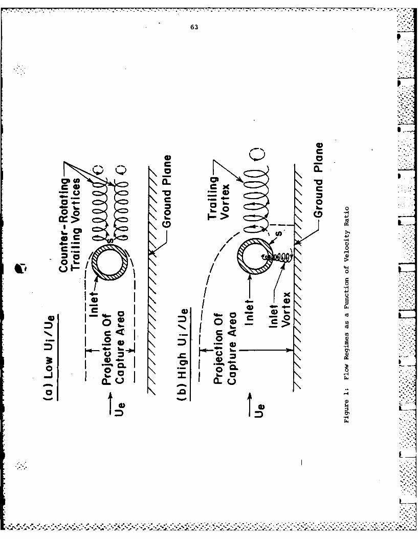
.o -:.
63
op
0Q 0
> C 4
-- CI
0\0
39 .0- 0:
'-4
5:4
64
xpo.5
'E-0
Ul
0
x -1
• -'-4,'.-.> .,,..,.
/- -.
(DU
- .... C1.
394
0 (n
-° '-U
o 0,o°
..",-. . . . . ., . ' . ' .. - - .- .. . . . . - . . .. , - .. . . . - .-.- . .-.- , . .- . "."..,.. .- . -.-. '
65
S0
o -4
ISUU)
l.4-c 0
44
--4
r14
44-
Pressure Tap 66
Locations (9) A' 30cm From Inlet Tip86
A-J TCylindrical
HInside Circulation Stnd
Measurement Station L
Inlet And Support
D; 15cm Inside Diameter
Path Used ForCirculationMeasurement
Five Hole ProbeTraversing Probe
T Three Hole Probe
K Kiel Probe
Section A-A S~ Static Tap
Figure 4: Inlet model (with measurement stations shown) and Location ofPath Used for Circulation Measurement
2 J " ___ __
67
N00
U))
cq--
h.4
E4
In
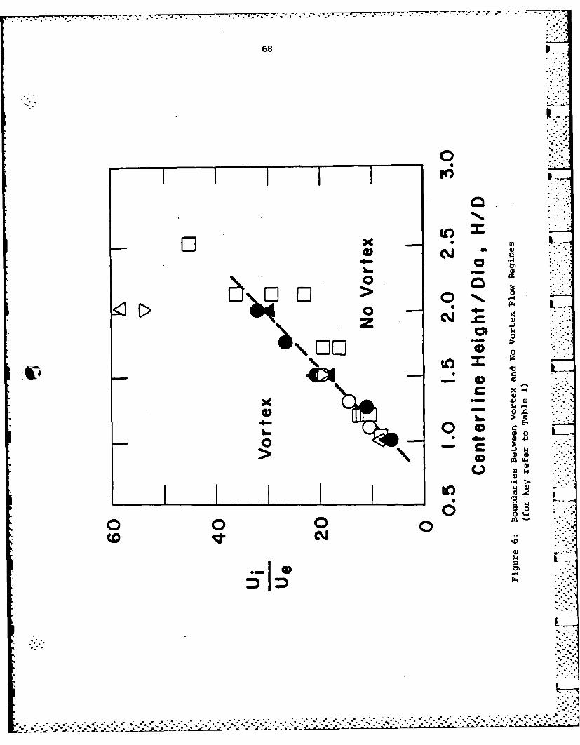
68
I~ 1-4
0.
- .- .
4-.-'.I
0
0 emo:.:-
g .
4444
0 4
x, -0
" ""
4-p
S
I
GIi
to
o
0--°oI
0 0
0 0
"
N° 0
.
-'.4 -.: ' :
p
-
.2-
° -
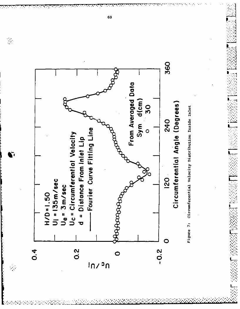
69
411
0 _ _'--'
0 ,.$o-
C
± o.jj.0.0_ -;.._ -
low
LL~
CF.7
",3 ' h .....
Lo 41. 0o
0 00" .'-)-N
- a l i-f-~~ - ...-.
*LO~h.'0 ° @
Xf* D mo
.,11!n/In :.On
II C,-='
I ",;@--3
i . -. --. . ' " -. "- . "- "- - . :.. ,-.'" .. . -. ... . : ... . ... . .... .. ... .. .... ..... ; - '..' . ... ....... '.0. . . -'
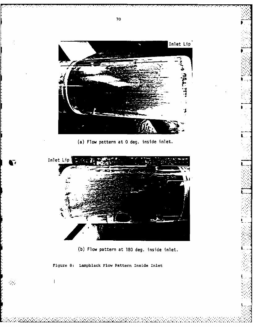
70
(a) Flow pattern at 0 deg. inside inlet.
(b) Flow pattern at 180 deg. inside inlet.
Figure 8: Lampblack Flow Pattern Inside Inlet
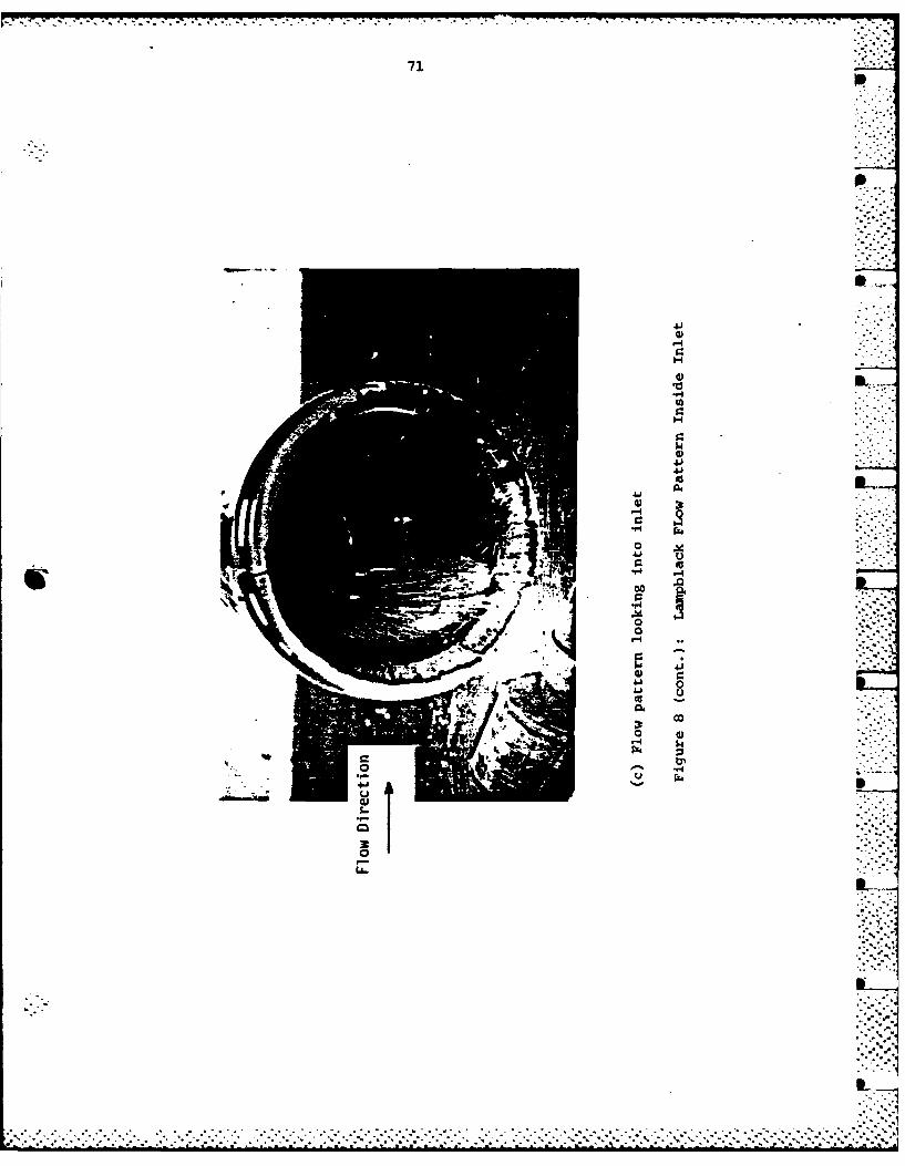
71
.41
-41
14
rA441
L6-
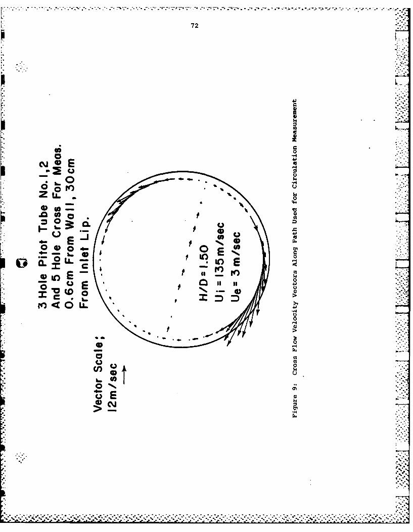
K 72
4J
VI 0
04
LL'000
'44
f4'
4I 004
03
% %J
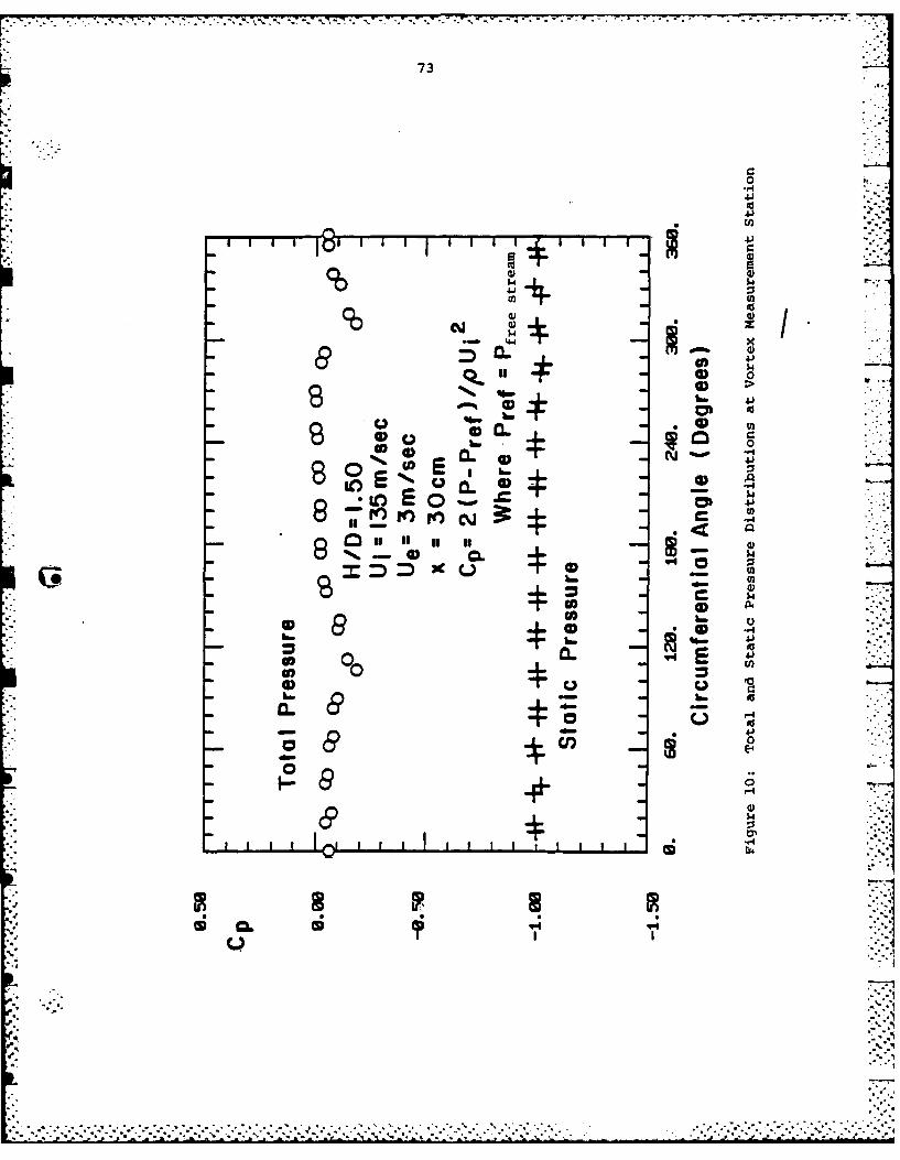
K~~~~ U.- - 7-
73
CL 4 J
4-)
0
IL b-
E o
rn 0e in,.
4* .': W*
9 o **4
m
-im )i ii mu 0
E-4-
.',S_ .':--'
0.:.-_:
.0. 0?.
• "-- h.
• , . . . . . . . o.
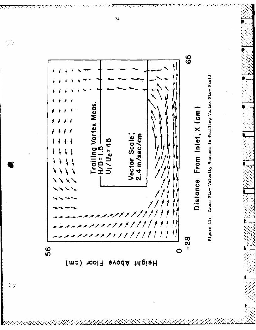
74
(0
r-4
*mo
0
III 4)
I>~%JAq
~ %.N >
Nk,
f/[I 0F
(WO) U)I ~qV469
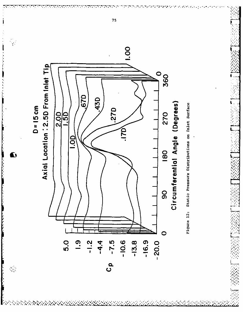
75
0
CL
0 0
clcn
O w
Ca,
CL.
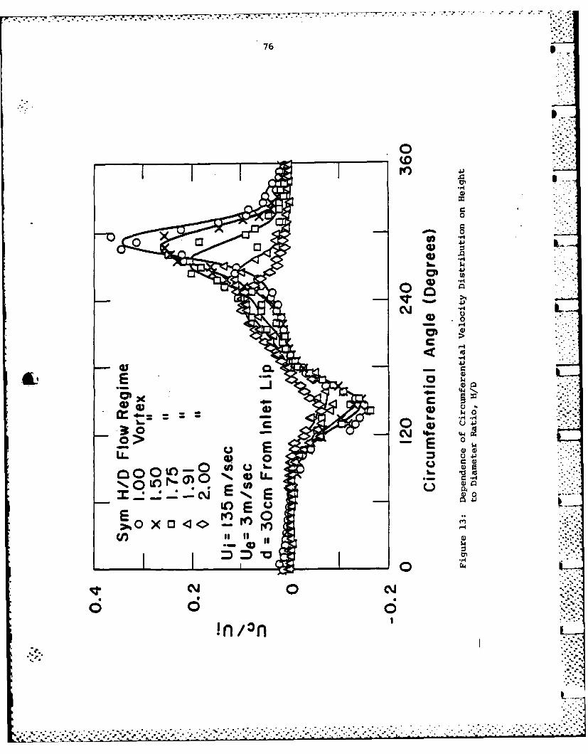
76
,0j
U0
ALI
'.4
EI 4)..I *4-I
0 *
04
c E~
0 -fo
- -0
o CM.Ir
30i /:On'
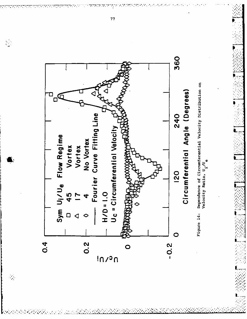
77
00
U
S,..,
N0 *0
.0- >
0 0 44
-) 44-,-
0 -WP . . .
-- ak° '
o CU 0 4
ci. '.?i?
U)) 0
< - 04 .)
") I -- 2.
. ., ,-..
C .0 44-
II -- --.
WL
n.. .. .
• -. o*-,- . .
. . ... . .. ...... . . . . .. .. * .. . .. .. , b.. ," . .' .. v . - v . ''''-.. ''''' .•.-.- " -" '''
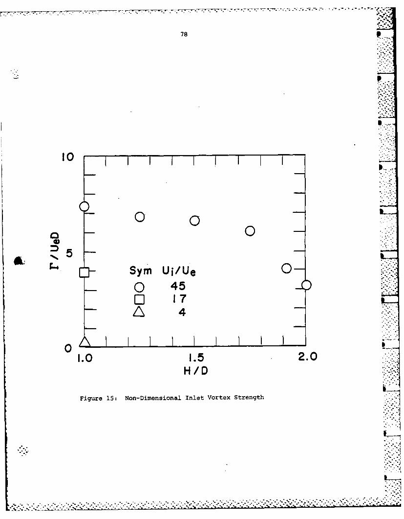
78
10 J
Sym Ui/Ue0o 45
r-1 17A 4
01.0 1.5 2.0
H/D
Figure 15: Non-Dimensional Inlet Vortex Strength
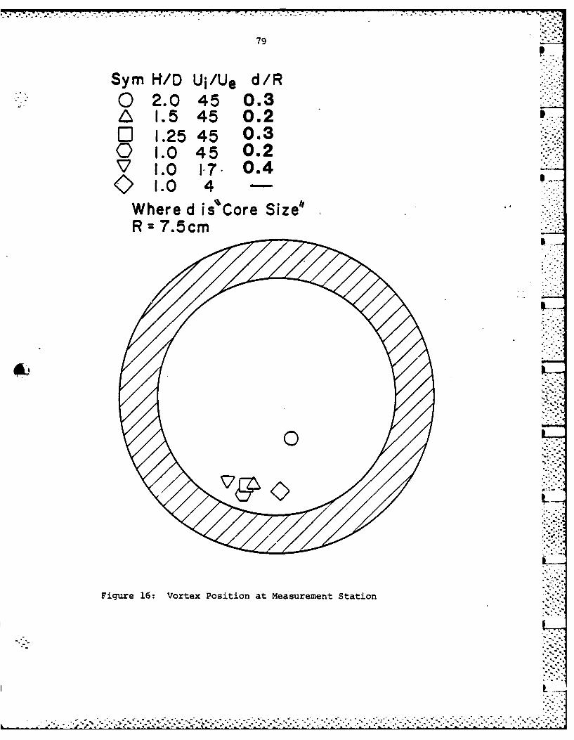
79
Sym 14/D UI/Ue d/R0 2.0 45 0.3A 1.5 45 0.2Ol 1.25 45 0.3o 1.0 45 0.2
K>1.0 4-Where d is* Core Size"#R =7.5cm
177
Figure 16: Vortex Position at Measurement Station
LI
........................ .. .. .. .. .. .. ...
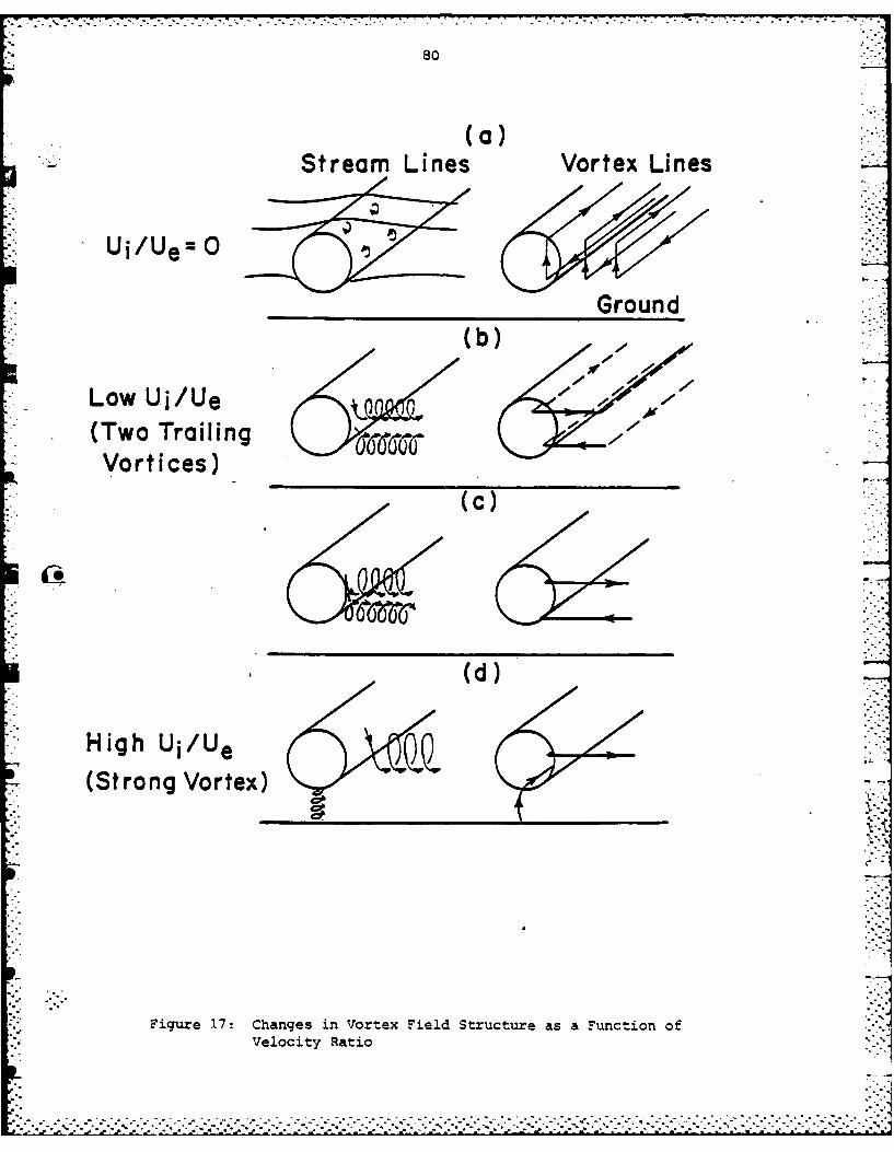
(a)Stream Lines Vortex Lines
Ui/Ue
Low Ui/Ue(Two TrailingVortices)
(d)
High Ui/Ue(Strong Vortex) Q I
Figure 17: Changes in Vortex Field Structure as a Function ofVelocity Ratio
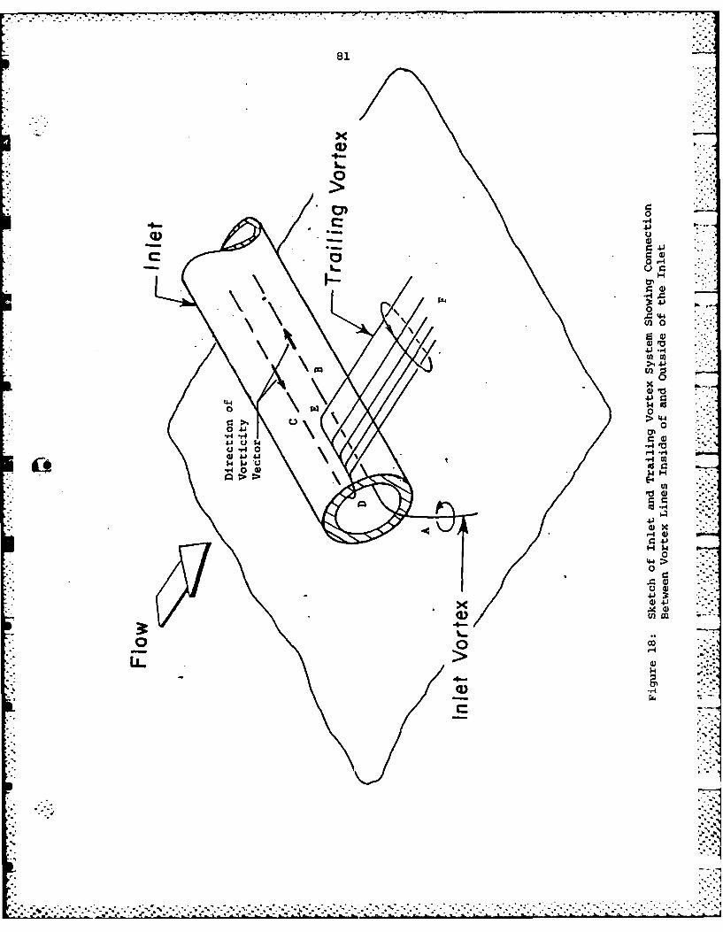
81
0 -
444
U)0
4 -,
W -3
go m
4J
0
(10
0 411
u -H 0
U-#4 0
*4J4.I W .
0
44 >
~4J
54
-. -- .- ' .
82
TASK IV: INVESTIGATION OF DISCRETE-BLADE AND THREE-DIMENSIONAL FLOWS
IN HIGHLY LOADED TURBOMACHINES
A. 3D FLOW AND DESIGN METHODS IN HIGHLY-LOADED TURBOMACHINES
Considerable progress has been made in the development of a blade
design technique for a 3D highly-loaded cascade subjected to sheared inlet
flow. The goal is an a priori blade design allowing for the effects of
secondary flow. To date the treatment is limited to inviscid, incompress-
ible flow in the limit of very thin blades.
The method used combines the best features of two alternative 3D
rotational flow descriptions: the "two-stream function" description, and
the Clebsch transformation technique. (In the former, the constants of
the motion are displayed best; in the latter, many of the field equations
are more convenient.) The requirement that the two descriptions yield
identical results provides useful computational information.
In both descriptions, the "smoothing technique" (4.*1), (4.2), developed
under this contract, is applied for cascades of large blade numbers (small
spacing). The result is a neat, closed theory (4.3) which allows us to
determine cascade blade shapes required to produce a specified result in
terms of cascade performance at high loading. Numerical examples are being
prepared to illustrate "good" and "bad" cases. A computer graphics presen-
tation is being developed to display the flow and blade results in a manner
to make them more understandable.
The method developed can also be used for analysis (performance)
calculations.
J..,
.......................... .. *.*
..... ~ ~ ~ , *..,.*. ,*-
83
B. NUMERICAL STUDIES OF SECONDARY FLOW IN A BEND USING SPECTRAL METHODS
Introduction
Two items will be described in this progress report: (1) the computer
code for the simulation of viscous flow in a bend of rectangular cross-
section using a mixed spectral finite-difference scheme; and (2) the formu-
lation of spectral element technique for the solution of the Navier-Stokes
equation in the bend with three elements: namely, an upstream element, a
bend element, and a downstream element.
(1) Mixed spectral finite difference code for viscous flow in a bend of
rectangular cross-section
This code has been designed in modular form. Each module performs a
particular task or computes a desired quantity. The strategy followed Is
that we first compute a basic flow with Vor - 0, Vo0 - V09(r,z),
Voz 0 satisfying the non-slip boundary condition at the inner wall r -
ri and the outer wall r - ro as well as the continuity and momentum
equations. This basic flow Vo(r,z) is time-independent. The time
dependent part and the three-dimensional part are contained in v so that
the resulting velocity field is described by V V0 (rz) + v(rGz°t).
Likewise, the pressure field may be similarly described. This is done for
convenience and is a procedure commonly used by research workers who
simulate turbulence and investigate transitional phenomena in fluid flows
(Refs. 4.4 and 4.5). Note that no approximation is implied by such a
description. Because we have assumed the flow to be incompressible,
*.%'
* ***"*.'**
...... ... o . ... . • . . . . . . . . . .. .
84
therefore a staggered finite difference grid system has to be used in the
direction of the bend so that the continuity condition can be satisfied in
consistence with the pressure field. Thus we would compute the tangential
velocity v at points Js 0 0,1,2,...J (the point J. - 0 would
correspond to the inflow boundary while the point Js - J corresponds to
the outflow boundary). However, for consistency we would compute the
velocity components Vr, vs, and the total pressure field Pt at the
finite difference grid points j lying hal:ay between two consecutive J..
The code consists of two essential parts:
(A) The preprocessing stage. Here the resolution of the simulation, the
geometrical parameters (i.e., the extent of the bend, the inner and outer
radii measured in units of half the bend height), the Reynolds number, the
inlet shear profile and the time step sizes are chosen. The main program
( PREPRO3 would call on:
(i) BASIC to compute the basic flow.
(ii) PREPRO to preprocess the first fractional step (the non-linear
convective step) by performing a LU decomposition of the tridiagonal
matrix operator for advancing each of the velocity components forward
in time.
(iii) PSNPRS to do the preprocessing necessary for the implementation of
the Poisson solver for the intermediate pressure field Pt in the
pressure correction step. To achieve this, PSNPRS would in turn call
on:
(a) PMEV to diagonalise the pressure Poisson operator in the 0-direc-
tion (i.e., the bend direction) with Dirichlet boundary condition
.. .. .. .. - o*.-..-..°..--*.. .. .. .
85
at 0 - 0 and the boundary condition pertaining to the second
derivative with respect to 0 at 0 = 00.
(b) ZNZV to diagonalise the pressure Poisson operator in the z-
direction with Noumann boundary conditions at z = ±1.
(c) COLRTH to compute the radial collocation operator resulting from
completion of (a) and (b) above. It is subsequently diagonalised-
incorporating the Neumann boundary condition at r = ri and r = ro.
(iv) PSNVEL to perform the preprocessing necessary for the Poisson solvers
that implement the viscous correction step. This PSNVEL would in . -
turn call on:
(a) PMEVEL to diagnonalise the velocity Poisson operator in the 0-..
direction vith Dirichlet boundary condition at 0 - 0 (inflow
boundary) and Neumann boundary condition at 0 - 0 (outflow
boundary).
(b) ZNEVEL to diagonalise the velocity Poisson operator in the z-
direction with Dirichlet boundary conditions at the walls z - ±1.
(c) COLRVR to compute the radial collocation operator that results
from the completion of (a) and (b) above for the radial velocity.
(d) COLRVT to compute the radial collocation operator that results
from the completion of (a) and (b) above for the tangential
velocity.
(e) COLRVZ to compute the radial collocation operator that results
from the completion of (a) and (b) above for the axial velocity.
The collocation operators of (c), (d) and (e) are each subsequently
diagonalised incorporating the Dirichlet boundary condition at the walls
.5___
86
r - ri and r - ro . Note that (c), (d) and (e) have to be done separately
because the radial part of the Poisson operators for the radial, the
tangential and the axial velocities are different due to the curvature term
in the equation of motion.
The results from this preprocessing stage are stored in data files
for use in the simulation stage to be described next.
(B) Simulation Stage. The main program BEND would call on:
Ci) DATAIN to read in data (including the initial condition on velocity
field) in files created during the preprocessing stage into the core
memory.
(ii) EULER which uses a simple Euler time-stepping scheme (the time-step
size for this step is much smaller compared to that specified for
the fractional stepping) to establish the values of velocity at two
initial time levels necessary for starting the fractional time
stepping of the Navier-Stokes equation. It also establishes the
initial vorticity field and the initial M-vector (-V x V x V) field.
(iii) PRESRE computes the intermediate pressure field Pt that imposes
the continuity condition.
Civ) VISCOS implements the viscous correction step that imposes the
non-slip boundary conditions at the walls.
(v) MOVVEL to keep two time levels of velocity components at any instant.
This is necessary for the two-time-level scheme used here as well as
for checking the approach to steady state solution if it exists. -
(vi) VOTICY to compute the vorticity field in the flow.
(vii) MOVMVT to keep two time levels of M-vector at any instance as
* ** . . . . . .-.. .-... ' . *4 .. * * *.. . .,
* ...-..-.. '..87
required by a two-time-level scheme.
(viii) MVECTR to compute the latest value of M-vector field.
(ix) DV1NTN to compute the tangential derivative of the velocity compon-
ents which will be used by SOURCi to calculate the RHS vector of the
operator equation that implements the convective step. The sub- a
routine module MOVDTN would perform a similar function to MOVVEL and
MOVMVT by keeping two time levels of the tangential derivative of
velocity compon-nts at any one instant.
x) (a) CONVEC to implement the nonlinear convective step.
(b) PRESRE to implement the pressure correction step.
(c) VISCOS to implement the viscous correction step.
The PRESRE would call or, PRSSLN which would in turn invoke BDYPSR,
PSPHIZ, PSTMTN and SOLPSN for the solution at the pressure step.
Similarly, VISCOS would call on:
(a) VRDSLN which would in turn invoke BDYVRD, VRPHIZ, VRTMIN and SOLVRD -. .
to obtain the radial velocity field.
(b) VTDSLN which would in turn invoke BDYVTN, VTPHIZ, VTTMTN and SOLVTN
to obtain the tangential velocity field.
(C) VZDSLN which would in turn invoke BDYVZ, VZPHIZ, VZTMTN and SOLVZ toe
obtain the axial velocity field.
Note that the tangential velocity corresponds to the velocity in the -.
direction of the bend while the radial and axial velocity constitute the
flow on the cross-sectional plane of the bend. Steps (v) to Cx) would be
repeated for advancing the flow forward in time.
At the moment, the subroutine module PRESRE (for the pressure
..-:,-:
88
- - correction step) has not been performing well in terms of accuracy as one
would expect. Currently work is directed at ascertaining the cause for the
loss in accuracy in PRESRE and a way of correcting that.
The inflow boundary conditions are specified while the outflow
boundary conditions assume either the first derivative or the second
derivative in the tangential direction vanishes.
(2) Formulation of Spectral Element Method
Work has begun on the formulation of spectral element technique for
the simulation of three-dimensional viscous flow. The formulation
described here was carried out while this co-investigator was at Whittle
Laboratory for a period of 5 weeks. For the flow in a bend, three macro-
elements are used: the element upstream of the bend, the bend element, and
the element downstream of the bend. Flow variables are expanded in a
triple Chebyshev series (i.e., the Chebyshev series is used as a high order
Lagrangian interpolant). Unwanted high resolution at the inflow and
outflow boundaries are eliminated via the introduction of multiple elements
in the flow direction. A Cartesian co-ordinate system is used in the .4... -.
upstream and the downstream element while a cylindrical co-ordinate system
is used in the bend element. Initial effort is focused on the solution of
Poisson and Helmholtz equations (as required for the pressure and viscous
steps in the solution of Navier-Stokes equation) in the multielements
domain. Each elemental domain is transformed to a standard domain in which
the boundaries of the domain are at -1 or +1. Diagonalisation of the
Poisson and the Helmholtz operators is performed in two orthogonal
directions on the cross-sectional plane. This reduces the original three-
, ..... . ..---.
89
dimensional equation into a one-dimensional one in the direction of the
bend. A variational principle in the bend-direction (or e-direction) is P
then invoked for building the elemental matrices. These elemental matrices
are then synthesized into a global matrix that satisfies the specified
inflow and outflow boundary conditions and preserves the continuity of
function at the elemental interfaces. It is hoped that in the future we
would be able to continue on this work so that an executable formulation
and analysis could be used to simulate viscous internal flow.
d' . -.
. .
• - -. ." - ., . ' - ' - / ' r- Z Z w- " rw . - -. -- i - - -.-.- --- .-- -.- - -.' -;" -;-.-- .- . ; _o I - " ' "
90
C. THREE-DIMENSIONAL BLADE DESIGN FOR LARGE DEFLECTION
Since publishing the work on the Cambridge design method (reference .
4.7), we can report some progress both on the application of the method and
on its improvement. The method has been applied in a simpler, but the same
fundamental, form to the design of a radial flow turbine by an industrial
firm. The results were very encouraging. Work is in progress on the
preparation of more rigorous methods for design-in turbomachines of arbi-
trary geometry, but with restriction to incompressible, irrotational flow
through the blades.
In our solution method (reference 4.8) we have divided the flow velo-
city into a mean velocity, averaged in the pitchwise or tangential direction,
and a periodic velocity. This periodic velocity is then expressed as a
Fourier series in the 0 or tangential direction. In the computation, the
• . Fourier series was truncated after some fifteen terms. The errors due to.
this truncation have been examined for the two-dimensional cascade and
found to arise from a term in the Fourier series which varies as 1/n2
where n is the harmonic. This term has been identified and a relatively
simple method of correcting the largest part of the truncation error is now
proposed. When applied to the two-dimensional cascade for which the Biot
Savart method gives the result of taking an infinite number of terms, it is
found that using 10 terms plus the truncation error correction gives a more
accurate answer than using 60 terms without truncation error correction.
The method has been extended to the full three-dimensional case and similar
results have been obtained. A report is in preparation.
Some numerical work has been done to examine in detail the blade
,* °N.*
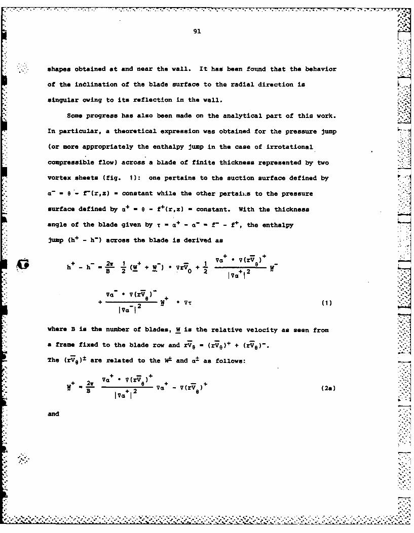
91
shapes obtained at and near the wall. It has been found that the behavior
of the indlination of the blade surface to the radial direction is
singular owing to its reflection in the wall.
Some progress has also been made on the analytical part of this work.
In particular, a theoretical expression was obtained for the pressure jump
(or more appropriately the enthalpy jump in the case of irrotational
compressible flow) across a blade of finite thickness represented by two
- vortex sheets (fig. 1): one pertains to the suction surface defined by
a -B - f-(r,z) = constant while the other pertaiLs to the pressure
surface defined by a+ e - f+(r,z) = constant. With the thickness
angle of the blade given by T a a+ - a f - f+, the enthalpy
jump (h+ - h-) across the blade is derived as
+ +
+2, w+ - V(rv h-h - (W+ + W)* r +-
B 2 0 2 v-"
Va * v(riV e+ -2 V(1
Iva-I
*where B is the number of blades, W is the relative velocity as seen from.7.
a frame fixed to the blade row and rve = (rVo)+ + (rV-."
The (r )± are related to the W1 and a± as follows:
oa V'(w 2,v + " (e + +: iV - iv* 1 0 + - v(r7V) (2a)B +2
and
, o7.
-. V.
92
-w - v2 va - v(r (2b)
(see Ref. 4.4)
It should be pointed out that the expression given in Eq. (1) does not
pertain to a point but rather to a fixed z on the r-9 plane (here we have
assumed that a right-handed cylindrical co-ordinate system is used). By
*letting T-0, we obtain the limit of infinitely thin blades where the
* enthalpy jump (h+ - h-) across the blade is given by
h W VrV (3)B -bl
where Wbl - 1/2(W + + W-). This agrees with the result obtained in Ref.
4.4. Following this, we can thus argue that the second term in the
i expression in Eq. (1) is a correction term due to the-fact that the blade
has a finite thickness. At this stage, we have not as yet adressed in
* rigor the question of whether Eq. (I) is valid when the flow upstream of
m the blade row is rotational. It should be kept in mind that the above
" results have been arrived at based on the assumptions that the flow is
- inviscid, homentropic and the rothalpy is uniform far upstream.
From the above analytical results, one would notice the slight increase
in complexity with the introduction of thickness into the blade. In the
case of infinitely thin blades, specification of the swirl schedule (rye)
in the blade region is sufficient for the determination of the blade shape.
However, for the case of blades with finite thickness, specification of only
one of (rV), (rvg)+ or (r0 )- is not sufficient. Some exploration
RD-Ri47 127 CURRENT PROBLEMS IN TURBOMACHINERY FLUID DYNAMICS(U) 2/2.MASSACHUSETTS INST OF TECH CAMBRIDGE GAS TURBINE ANDPLASMA DYNAMICS LAB E M GREITZER ET AL. JUN 84
UNCLASSIFIED AFOSR-TR-84-859 F49628-82-K-8882 F/G 29/4 NLlmmmnnm7
11111 -iL2
I" ___0
1111-6w
I~I~I7 *
93L
* -- of the possibilities has been done for the example of two-dimensional
cascades. Strut profiles have been computed using the Biot Savart method
and various distributions of (rV9 )+ (note for the case of the strut
(rV 8 ) - (r7)-). For cambered blades it may be better to specify
rV9 and T. For instance, one could conceive of the design calculation
as follows:
(1) Specify V[-(rV90)+ + ( )-] and the thickness angle Tr
(2) Guess an initial a- (hence a+)
(3) Determine (rvg)" (hence (rV0 )+) approximately from Eq. (2b)
assuming a value of W- from an approximate mean flow calculation
(4 Compute the flow field with the knowledge of a+, 7, (re)+ and
(Cry)
(5) Update a- using the boundary condition on the suction surface that
W- * Va- 0
(6) Update (rV) using Eq. (2a) hence (rV9) or W+ * Va+ - 0
(7) Repeat steps (3) to (6) until convergence is obtained
Notice that in the above procedure, we have allowed (rV0 )+ and (rV0 )-
to float in such a way that their sum agrees with the specified (r).
A different procedure from the above could have been followed by
specifying ( ) and T but allowing (r 9) and (r 1+ to
float such that their difference is (rV'). Alternatively, there
may be the possibility of specifying the enthalpy distribution and
thickness angle T. We believe these many design procedures could be
arrived at using the above analytical results. We have not examined in
detail the implications of devising such a design procedure.
-1 7.5
94
No effort has been expended on developing numerical techniques and
designing a computer code -to implement any numerical calculations based on
the above extension of the theory.
1
_ .% IEE J . . I kI. % % I!I. .. I = .! - . P.' *- .-.- *- . - - °% -. " -. - -.- - - - - -.
95
References:
4.1 McCune, J.E., and Dang, T.Q., "Periodic Internal Flows," presented atthe Symposium on "Computation of Internal Flows: Methods and Applications,"February 11-17, 1984, Now Orleans.
4.2 Dang, T.Q., and McCune, J.E., "Design Method for Highly-Loade Bladeswith Blockage in Cascade," presented at the Symposium on "Computation of.Internal Flows: Methods and Applications," February 11-17, 1984, NowOrleans.
4.3 Dang, T.Q., and McCune, J.E., "A 3D Blade Design Method in RotationalFlow," to be presented at the "International Conference on Inverse DesignConcepts in Engineering Sciences (ICIDES)," October 17-18, 1984, Universityof Texas at Austin.
4.4 S. Orszag and L. Kells, "Transition to turbulence in plane poiseuilleand plane couette flow," JFM (1980), Vol. 96, Pt. 1.
4.5 A. Patera and S. Orszag, "Finite-amplitude stability of axisymmetricpipe flow," JFM (1981), Vol. 112.
4.6 Previous Multi-Investigator Progress Reports.
4.7 C.S. Tan, et al., "Three-dimensional blade design for large deflec--tions using an analytical theory," GTL Report No. 118, and CUED/A-Turbo/
TR115, 1982.
4.8 Hawthorne, W.R., Tan, C.S., et al., "Theory of Blade Design for LargeDeflections, Part I - Two-Dimensional Cascades, and Part II - AnnularCascades," ASME J. Eng. for Gas Turbines and Power, 106, pp. 346-365,April 1984.
.. % .... **'% %** *** . . .
96
* GENERAL PROGRESS ON AFRAPT
The Air Force OSR sponsored educational program, called Air Force
Research in Aeronautical Propulsion Technology (AFRAPT), steering
committee consists of:
Dr. Michael Salkind APOSR, Chairman
Mr. Walter Schrader AVCO Lycoming
Dr. Lynn Snyder DDA
Mr. Elmer Wheeler Garrett Aerospace Corp.
Dr. Fred Erich GE Lynn
Dr. David Wisler GE Evendale
Mr. Tom Hampton Pratt & Whitney (GPD)
Professor Sandford Fleeter Purdue University
Professor Peter Jenkins Texas A&M University
and
Professor Eugene E. Covert Massachusetts Instituteof Technology, Secretary
In the past year this group has met twice. The annual brochure has
been prepared and is being distributed. The primary business is that of
trying to establish procedures to meet the needs and schedules of all
participants.
The Steering Committee has met, reviewed the program and accepted
modified procedures with the goal of balancing the number of vacancies in
the program between the industry and the university.
7.:.~* .~ *. .~ .* ** ~ . . .* * . *" -.S* *
97
3. PUBLICATIONS
Chang, P., Prell, N.E., Greitzer, E.M., Tan, C.S., "Effects ofCompressor Hub Treatment on Stator Stall and Pressure Rise," J. Aircraft,.21, pp. 469-475, July 1984.
Hawthorne, W.R., Wang, C., Tan, C.S., and McCune, J.E., "Theory ofBlade Design for Large Deflections, Part I: Two-Dimensional Cascades,"ASME Journal for Engineering for Power, 106, pp. 346-354, April 1984.
Tan, C.S., Hawthorne, W.R. McCune, J.E., and Wang, C., "Theory ofBlade Design for Large Deflections, Part II: Annular Cascades,"ASME Journal for Engineering for Power, 106, pp. 354-366, April 1984.
Liu, W., Greitzer, E.M., and Tan, C.S., "Surface Static Pressuresin an Inlet Vortex Flow Field," (presented at 1984 ASME Gas TurbineConference), to be published in ASME J. Engineering for Power.
Ng, W.F., and Epstein, A.H., "High Frequency Temperature Probefor Unsteady Compressible Flows," Review of Scientific Instruments, 54,pp. 1678-1683, December 1983.
Ng, W.F. and Epstein, A.H., "Unsteady Losses in TransonicCompressors," (presented at 1984 ASME Gas Turbine Conference), accepted
- for publication in ASME J. Engineering for Power.
Tan, C.S. and Greltzer, E.M., "Non-Axisymmetric Compressible Swirling* Flow in Turbomachine Annuli," to be submitted to AIAA Journal.
.. 'd.;
* . * - *-. °-
,.*~,i*.**I*...*....* *.....*.*,*...,~*.**.*..*..**-**-*. . . . . . ._... -:.* . . . . . . . . . ."" t ...
- 98
4. PROGRAM PERSONNEL
Principal Investigators:
Jack L. Kerrebrock
R.C. Maclaurin Professorand Department ReadAeronautics and Astronautics
Edward M. Greitzer 6Professor of Aeronautics and AstronauticsDirector, Gas Turbine Laboratory
William T. Thompkins, Jr.Associate Professor of Aeronautics and Astronautics
James E. McCuneProfessor of Aeronautics and Astronautics
Co-Investigators:
Alan H. EpsteinAssociate Professor of Aeronautics and AstronauticsAssociate Director, Gas Turbine & Plasma Dynamics Laboratory
Choon S. Tan
Research Associate
Collaborating Investigators:.
Eugene E. CovertProfessor of Aeronautics and AstronauticsDirector, Center for Aerodynamic Studies
Sir William R. HawthorneSenior Lecturer
Wai K. ChengSoderberg Assistant Professor of Mechanical Engineering
Hyoun-Woo ShinPost-Doctoral Associate
Robert HaimesResearch Associate
.... ,
i ~ i '. 1% .-. "'. ',.',. ,' '" -' ."%" '.." ":" '-" ."". : ". "" ." " " ". -", ." "• " -. '.", . '.'..'. -".' .' -' "- .':..'-",". ,"-
99
Current Graduate Research Assistants:
9/83 - Present Mark Johnson (APRAPT Student)I9/81 - Present Thong Daflg*9/80 - 12/83 Wing-Fal Ng**9/83 - Present Petros Kotidis9/82 - 3/84 Cheryl Shippee*9/82 - 12/83nt Gilles Thevenet*9/79 - 6/84 Siu Shing Tong**
S.M4. Degree Completed**Ph.D Thesis Completed
FL *
V, P. 0-7i
100
5. INTERACTIONS
" Presentations
E.M. Greitzer, "Mechanisms of Inlet Vortex Formation," CambridgeUniversity, November 1983, and British Aerospace Corporation, February 1984.
E.M. Greitzer, "The Stability of Pumping Systems," Rolls-RoyceLimited, Derby, England, December 1983.
E.M. Greitzer, "Stability Enhancement Using Casing/Hub Treatment,"Cambridge University, December 1983.
E.M. Greitzer, "Introduction to Unsteady Flows in Turbomahcines" andwFlov Instabilities in Turbomachines and Gas Turbine Engines," lectures
presented at Von Karman Institute, course on Unsteady Flows in Turbo-machines, February 1984.
E.M. Greitzer, "MIT Research on Stall Recovery," a progress report pre-:sented to Pratt & Whitney Aircraft, Government Products Division, March 1984.
C.S. Tan, "Spectral Method Computations of Internal Flows," Cambridge
University, April 1984.
Dang, T.Q. and McCune, J.E., "Periodic Internal Flows," presented at
. ASME Symposium on "Computation of Internal Flows: Methods andSApplications," Feb. 11-17, 1984, New Orleans.
Dang, T.Q., McCune, J.E., "Design Method for Highly-Loaded Blades withBlockage in Cascade," presented at ASNE Symposium on "Computation ofInternal Flows: Methods and Applications," Feb. 11-17, 1984.
As described in previous reports, there are strong interactions between theGas Turbine Laboratory and the aircraft engine industry, as well as AirForce and other government laboratories. We also have an active seminarprogram to bring speakers from industry and/or government to MIT. Duribgthe past six months theme have included:
Dr. Robert Dring, Manager, Gas Turbine Technology,United Technologies Research Center,"An Overview of Axial Compressor Aerodynamics"
Mr. Michael Pierzga, Research EngineerU.S. Army Propulsion Laboratory"Investigation of the Three-Dimensional Flow Field Within aTransonic Fan Rotor - Experiment and Analysis"
7.
Dr. S. Srinivasan, Manager of Applied Mechanics ResearchUnited Technologies Research Center*Aerodynamically Excited Vibrations of a Part Span Shrouded Fan"
Dr. Arthur 3. Wennerstrom
Air Force Aeropropulsion Laboratory"Design Techniques for High Performance Pans and Compressors"
- ./: . . . ' .. .. .. ., . ... . ........ .. % %.* . . % .. .,. .. ........ ..,....- . , .. •
101
6. DISCOVERIES, INVENTIONS, AND SCIENTIFIC APPLICATIONS "-
IDuring the present contract period, there have been no iLnventions. ,.
.
o$.,
*-'o
a ~'V . %~f %~) ~ 4 ~ .. *- %'*%.*
- - *. .
102
7. CONCLUSIONS
As we have stated previously, although the emphasis in work done
varies from project to project, we do appear to be making continued progress
in all of the efforts. One further aspect deserves mention. This past
year we had our first AFRAPT student, Mr. M. Johnson. Our involvement in .
the program has now expanded and Mr. D. Fink (associated with General
Electric) and Ms. J. Koo (AVCO), who are currently students at MIT, will
also be starting in this program this summer.
.+ * . .
<'NE
It t


![SotC SRD - Fate · SotC SRD SotC SRD Spirit of the Century (OGL SRD) ... °On Top Of It ... °Heart’s Secret [Empathy]](https://img.pdfslide.net/doc/110x75/5b367e717f8b9aec518e8e59/sotc-srd-sotc-srd-sotc-srd-spirit-of-the-century-ogl-srd-on-top-of.jpg)