SSA-based Register Allocation with PBQP

Sebastian Buchwald, Andreas Zwinkau, and Thomas Bersch

Karlsruhe Institute of Technology (KIT){buchwald,zwinkau}@kit.edu thomas.bersch@student.kit.edu

Abstract. Recent research shows that maintaining SSA form allows tosplit register allocation into separate phases: spilling, register assign-ment and copy coalescing. After spilling, register assignment can bedone in polynomial time, but copy coalescing is NP-complete. In this pa-per we present an assignment approach with integrated copy coalescing,which maps the problem to the Partitioned Boolean Quadratic Problem(PBQP). Compared to the state-of-the-art recoloring approach, this re-duces the relative number of swap and copy instructions for the SPECCINT2000 benchmark to 99.6% and 95.2%, respectively, while taking19% less time for assignment and coalescing.

Keywords: register allocation, copy coalescing, PBQP

1 Introduction

Register allocation is an essential phase in any compiler generating native code.The goal is to map the program variables to the registers of the target archi-tecture. Since there are only a limited number of registers, some variables mayhave to be spilled to memory and reloaded again when needed. Common regis-ter allocation algorithms like Graph Coloring [3,6] spill on demand during theallocation. This can result in an increased number of spills and reloads [11]. Incontrast, register allocation based on static single assignment (SSA) form allowsto completely decouple the spilling phase. This is due to the live-range splitsinduced by the φ-functions, which render the interference graph chordal andthus ensure that the interference graph is k-colorable, where k is the maximumregister pressure.

The live-range splits may result in shuffle code that permutes the values (asvariables are usually called in SSA form) on register level with copy or swapinstructions. To model this circumstance, affinities indicate which values shouldbe coalesced, i.e. assigned to the same register. If an affinity is fulfilled, insertingshuffle code for the corresponding values is not necessary anymore. Fulfilling suchaffinities is the challenge of copy coalescing and a central problem in SSA-basedregister allocation.

In this work we aim for a register assignment algorithm that is aware of affini-ties. In order to model affinities, we employ the Partitioned Boolean QuadraticProblem (PBQP), which is a generalization of the graph coloring problem.

In the following, we

– employ the chordal nature of the interference graph of a program in SSA formto obtain a linear PBQP solving algorithm, which does not spill registers,but uses a decoupled phase instead.

– integrate copy coalescing into the PBQP modelling, which makes a separatephase afterwards unnecessary.

– develop a new PBQP reduction to improve the solution quality by mergingtwo nodes, if coloring one node implies a coloring of the other one.

– introduce an advanced technique to handle a wide class of register constraintsduring register assignment, which enlarges the solution space for the PBQP.

– show the competitiveness of our approach by evaluating our implementationfor quality and speed. Additionally, some insight into our adaptations isgained by interpreting our measurements.

In Section 2 we describe related register allocation approaches using eitherSSA form or a PBQP-based algorithm, before we combine both ideas in Sec-tion 3, which shows the PBQP algorithm and our adaptations in detail. Section 4presents our technique to handle register constraints. Afterwards, an evaluationof our implementation is given in Section 5. Finally, Section 6 describes futurework and Section 7 our conclusions.

2 Related Work

2.1 Register allocation on SSA form

Most SSA-based compilers destruct SSA form in their intermediate represen-tation after the optimization phase and before the code generation. However,maintaining SSA form provides an advantage for register allocation: Due to thelive-range splits that are induced by the φ-functions, the interference graph ofprograms in SSA form is chordal [4,1,13], which means every induced subgraphthat is a cycle, has length three. For chordal graphs the chromatic number isdetermined by the size of the largest clique. This means that the interferencegraph is k-colorable, if the spiller has reduced the register pressure to at mostk at each program point. Thus, spilling can be decoupled from assignment [13],which means that the process is not iterated as with Graph Coloring.

To color the interference graph we employ the fact that there is a perfectelimination order (PEO) for each chordal graph [7]. A PEO defines an ordering< of nodes of a graph G, such that each successively removed node is simplicial,which means it forms a clique with all remaining neighbors in G. After spilling,assigning the registers in reverse PEO ensures that each node is simplicial andthus has a free register available. Following Hack, we obtain a PEO by a post-order walk on the dominance tree [11].

In addition to φ-functions, live-range splits may originate from constrainedinstructions. For instance, if a value is located in register R1, but the constrainedinstruction needs this value in register R2, we can split the live-range of this

value. More generally, we split all live-ranges immediately before the constrainedinstruction to allow for unconstrained copying of values into the required registersand employ copy coalescing to remove the overhead afterwards. With this inmind, we add affinity edges to the interference graph, which represent that theincident nodes should be assigned to the same register. Each affinity has assignedcosts, which can be weighted by the execution frequency of the potential copyinstruction. The goal of copy coalescing is to find a coloring that minimizesthe costs of unfulfilled affinities. Bouchez et al. showed that copy coalescing forchordal graphs is NP-complete [1], so one has to consider the usual tradeoffbetween speed and quality.

Grund and Hack [10] use integer linear programming to optimally solve thecopy coalescing problem for programs in SSA form. To keep the solution timebearable some optimizations are used, but due to its high complexity the ap-proach is too slow for practical purposes.

In contrast, the recoloring approach from Hack and Goos [12] features aheuristic solution in reasonable time. It improves an existing register assign-ment by recoloring the interference graph. Therefore, an initial coloring can beperformed quickly without respect to quality. To achieve an improvement, thealgorithm tries to assign the same color to affinity-related nodes. If changingthe color of a node leads to a conflict with interfering neighbors, the algorithmtries to solve this conflict by changing the color of the conflicting neighbors. Thiscan cause conflicts with other neighbors and recursively lead to a series of colorchanges. These changes are all done temporarily and will only be accepted, if avalid recoloring throughout the graph is found.

Another heuristic approach is the preference-guided register assignment in-troduced by Braun et al. [2]. This approach works in two phases: in the firstphase the register preferences of instructions are determined and in the secondphase registers are assigned in consideration of these preferences. The preferencesserve as implicit copy coalescing, such that no extra phase is needed. Further-more, the approach does not construct an interference graph. Preference-guidedregister assignment is inferior to recoloring in terms of quality, but significantlyfaster.

2.2 PBQP-based register allocation

The idea to map register allocation to PBQP was first implemented by Scholzand Eckstein [16] and features a linear heuristic. Since their implementation doesnot employ SSA form, they need to integrate spilling into their algorithm. Hamesand Scholz [14] refine the approach by presenting a new heuristic and a branch-and-bound approach for optimal solutions. The essential advantage of the PBQPapproach is its flexibility, which makes it suited for irregular architectures.

3 PBQP

3.1 PBQP in general

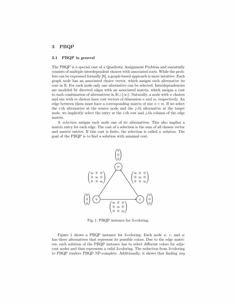
The PBQP is a special case of a Quadratic Assignment Problem and essentiallyconsists of multiple interdependent choices with associated costs. While the prob-lem can be expressed formally [8], a graph-based approach is more intuitive. Eachgraph node has an associated choice vector, which assigns each alternative itscost in R. For each node only one alternative can be selected. Interdependenciesare modeled by directed edges with an associated matrix, which assigns a costto each combination of alternatives in R∪{∞}. Naturally, a node with n choicesand one with m choices have cost vectors of dimension n and m, respectively. Anedge between them must have a corresponding matrix of size n×m. If we selectthe i-th alternative at the source node and the j-th alternative at the targetnode, we implicitly select the entry at the i-th row and j-th column of the edgematrix.

A selection assigns each node one of its alternatives. This also implies amatrix entry for each edge. The cost of a selection is the sum of all chosen vectorand matrix entries. If this cost is finite, the selection is called a solution. Thegoal of the PBQP is to find a solution with minimal cost.

u v

w

000

000

000

∞ 0 00 ∞ 00 0 ∞

∞ 0 00 ∞ 00 0 ∞

∞ 0 00 ∞ 00 0 ∞

Fig. 1: PBQP instance for 3-coloring.

Figure 1 shows a PBQP instance for 3-coloring. Each node u, v, and whas three alternatives that represent its possible colors. Due to the edge matri-ces, each solution of the PBQP instance has to select different colors for adja-cent nodes and thus represents a valid 3-coloring. The reduction from 3-coloringto PBQP renders PBQP NP-complete. Additionally, it shows that finding any

PBQP solution is NP-complete, since each solution is optimal. However, our al-gorithm can still solve all of our specific problems in linear time as we show inSection 3.4.

3.2 PBQP construction

As mentioned above, SSA-based register allocation allows to decouple spillingand register assignment, such that register assignment is essentially a graphcoloring problem. In Figure 1 we show that PBQP can be considered as a gener-alization of graph coloring by employing color vectors and interference matrices:

Color vector The color vector contains one zero cost entry for each possiblecolor. (

0 0 0)T

Interference matrix The matrix costs are set to∞, if the corresponding colorsare equal. Otherwise, the costs are set to zero.∞ 0 0

0 ∞ 00 0 ∞

Register allocation can be considered as a graph coloring problem by iden-

tifying registers and colors. In order to integrate copy coalescing into registerassignment, we add affinity edges for all potential copies, which should be pre-vented.

Affinity matrix The matrix costs are set to zero if the two corresponding regis-ters are equal. Otherwise, the costs are set to a positive value that representsthe cost of inserted shuffle code. 0 1 1

1 0 11 1 0

A PBQP instance is constructed like an interference graph by inspecting the

live-ranges of all values. The values become nodes and get their correspondingcolor vectors assigned. For each pair of interfering nodes an interference matrix isassigned to the edge between them. Likewise, the affinity cost matrix is assignedto an edge between a pair of nodes, which should get the same register assigned.If a pair of nodes fulfills both conditions, then the sum of both cost matrices isassigned. While the copy cannot be avoided in this case, there may still be costdifferences between the register combinations.

3.3 Solving PBQP instances

Solving the PBQP is done by iteratively reducing an instance to a smaller in-stance until all interdependencies vanish. Without edges every local optimum is

also globally optimal, so finding an optimal solution is trivial (unless there isnone). By backpropagating the reductions, the selection of the smaller instancecan be extended to a selection of the original PBQP instance. Originally, thereare four reductions [5,9,16]:

RE: Independent edges have a cost matrix that can be decomposed into twovectors u and v, i.e. each matrix entry Cij has costs ui + vj . Such edgescan be removed after adding u and v to the cost vector of the source andtarget node, respectively. If this would produce infinite vector costs, thecorresponding alternative (including matrix rows/columns) is deleted.

R1: Nodes of degree one can be removed, after costs are accounted in theadjacent node.

R2: Nodes of degree two can be removed, after costs are accounted in thecost matrix of the edge between the two neighbors; if necessary, the edge iscreated first.

RN: Nodes of degree three or higher. For a node u of maximum degree weselect a locally minimal alternative, which means we only consider u and itsneighbors. After the alternative is selected, all other alternatives are deletedand the incident edges are independent, so they can be removed by usingRE.

RE, R1, and R2 are optimal in the sense that they transform the PBQPinstance to a smaller one with equal minimal costs, such that each solution ofthe small instance can be extended to a solution of the original instance withequal costs. For sparse graphs these reductions are very powerful, since theydiminish the problem to its core. If the entire graph can be reduced by thesereductions, then the resulting PBQP selection is optimal. If nodes of degree threeor higher remain, the heuristic RN ensures linear time behavior.

Hames et al. [14] introduced a variant of RN that removes the correspondingnode from the PBQP graph without selecting an alternative. Thus, the decisionis delayed until the backpropagation phase. We will refer to this approach as latedecision. The other approach is early decision, which colors a node during RN.In this paper we follow both approaches and we will show which one is moresuitable for SSA-based register allocation.

3.4 Adapting the PBQP solver for SSA-based Register Allocation

In the context of SSA-based register allocation, coloring can be guaranteed tosucceed, if done in reverse PEO with respect to the interference graph. Thisseems to imply that our PBQP solver must assign registers in reverse PEO.However, we show in the following that this restriction is only necessary forheuristic reductions. Therefore, choosing a node for heuristic decision must usethe last node of the PEO for early decision and the first node of the PEO for latedecision. This different selection of nodes is needed, because the backpropagationphase inverts the order of the reduced nodes.

Early application of optimal reductions There is a conflict between thenecessity to assign registers in reverse PEO and the PBQP strategy to favorRE, R1, and R2 until only RN is left to apply. Fortunately, we can show thatthe application of this reductions preserves the PEO property with Theorem 1below.

Lemma 1. Let P be a PEO of a graph G = (V,E) and H = (V ′, E′) an inducedsubgraph of G, then P |V ′ is a PEO of H.

Proof. For any node v ∈ H let Vv = {u ∈ NG(v) | u > v} be the neighbor nodesin G behind in P and respectively V ′

v = {u ∈ NH(v) | u > v}. By definitionV ′v ⊆ Vv. Vv is a clique in G, therefore V ′

v is a clique in H and v is simplicial,when eliminated according to P |V ′ . ut

From Lemma 1 we know, that R1 preserves the PEO, since the resultinggraph is always an induced subgraph. However, R2 may insert a new edge intothe PBQP graph.

Lemma 2. Let P be a PEO of a graph G = (V,E) and v ∈ V a vertex of degreetwo with neighbors u,w ∈ V . Further, let H=(V’,E’) be the subgraph induced byV \ {v}. Then P |V ′ is a PEO of H ′ = (V ′, E′ ∪ {{u,w}}).

Proof. If {u,w} ∈ E this follows directly from Lemma 1, since no new edge isintroduced. In the other case, we assume without loss of generality u < w. Since{u,w} 6∈ E, v is not simplicial and we get u < v. Therefore, the only neighbornode of u in H behind in P must be v. Within H ′ the node w is the only neighborof u behind in the PEO, hence u is simplicial. For the remaining nodes v and wthe lemma follows directly from Lemma 1. ut

With Lemma 2 the edge inserted by R2 is proven harmless, so we can derivethe necessary theorem now. Remember that the PEO must be derived from theinterference graph, while our PBQP graph may also include affinity edges.

Theorem 1. Let G = (V,E) be a PBQP graph, i(E) the interference edges inE, i.e. edges that contain at least one infinite cost entry, P a PEO of (V, i(E))and H = (V ′, E′) the PBQP graph G after exhaustive application of RE, R1 andR2. Further, let Ei be the interference edges that are reduced by RE. Then, P |V ′

is a PEO of (V ′, i(E′) ∪ Ei).

U

V

W

Y

(R0R1

)

(R0R1

)

R0R1R2

(∞ 00 ∞

)

(∞ 0 00 ∞ 0

)

(∞ 0 00 ∞ 0

)(0 1 11 0 1

)

(a) PBQP instance that cannot be reducedfurther by RE, R1 or R2.

U W

Y

(R0R1

) R0R1R2

(∞ ∞ 0∞ ∞ 0

)

(1 0 10 1 1

)

(b) PBQP instance after merging Vinto U .

Fig. 2: Example of an RM application.

Proof. If at least one affinity edge is involved in a reduction, there is no newinterference edge and we can apply Lemma 1. If we consider only interferenceedges, Lemma 1 handles R1 and Lemma 2 handles R2. Applying RE for aninterference edge moves the interference constraint into incident nodes. Thus,we have to consider such edges Ei for the PEO. ut

Merging PBQP nodes The PBQP instances constructed for register assign-ment contain many interference cliques, which cannot be reduced by optimalreductions. This implies that the quality of the PBQP solution highly dependson the RN decisions. In this section we present RM, a new PBQP reduction thatis designed to improve the quality of such decisions.

Figure 2a shows a PBQP instance that cannot be further reduced by ap-plication of RE, R1 or R2. Hence, we have to apply a heuristic reduction. Weassume that the PEO selects U to be the heuristically reduced node. The newreduction is based on the following observation: If we select an alternative atU , there is only one alternative at V that yields finite costs. Thus, a selectionat U implicitly selects an alternative at V . However, the affinities of V are notconsidered during the reduction of U . The idea of the new reduction is to mergethe neighbor V into U . After the merge, U is also aware of V ’s affinities whichmay improve the heuristic decision.

To perform the merge, we apply the RM procedure of Algorithm 1 witharguments v = V and u = U . In line 2 the algorithm chooses w = Y as adjacent

Algorithm 1 RM merges the node v into the node u. The notation is adoptedfrom [16].Require: a selection at u implies a specific selection at v.1: procedure RM(v, u)2: for all w ∈ adj(v) do3: if w 6= u then4: for i← 1 to |cu| do5: c← 06: if cu(i) 6=∞ then7: iv ← imin(Cuv(i, :) + cv)8: c← Cvw(iv, :)

9: ∆(i, :)← c

10: Cuw ← Cuw +∆11: remove edge (v, w)

12: ReduceI(v)

node. We now want to replace the affinity edge (v, w) by an edge (u,w). In lines4–9 we create a new matrix ∆ for the edge (u,w). To construct this matrix weuse the fact that the selection of an alternative i at u also selects an alternative ivat v. Thus, the i-th row of ∆ is the iv-th row of Cuw. For our example this meansthat we have to swap the rows for R0 and R1 in order to obtain ∆ from Cvw.Since (u,w) does not exist, we create the edge with the matrix ∆. Afterwardswe delete the old edge (v, w).

In the next iteration, the algorithm chooses w =W as adjacent node. Similarto the previous iteration, we compute the matrix ∆. Since the edge (u,w) exists,we have to add ∆ to the matrix Cuw. After the deletion of (v, w), the nodev has degree one and can be reduced by employing R1. Figure 2b shows theresulting PBQP instance. Due to the merge the edge (U,W ) is independent.After removing the edge the PBQP instance can be solved by applying R1 andR2, leading to an optimal solution.

Although RM is an optimal reduction, we only apply it immediately beforea heuristic reduction at a node U . If there is a neighbor V of U that can bemerged into U we apply RM for these two nodes. This process iterates until nosuch neighbor is left. In some cases—like our example—the RM allows furtheroptimal reductions that supersede a heuristic reduction at U . If U still needs aheuristic reduction, the neighbors of the merged nodes are also considered bythe heuristic and thus can improve the heuristic decision.

The reason for applying RM only immediately before a heuristic decision at anode u is that in this case each edge is reassigned only once, due to the fact thatthe node u (and all incident edges) will be deleted after the merge. Thus, eachedge is considered at most twice: once for reassignment, and once during thereduction of u. As a result, the overall RM time complexity is in O(mk2) wherem = |E| is the number of edges in the PBQP graph and k is the maximumnumber of alternatives at a node. The same argument can be used to showthat the overall RN time complexity is in O(mk2). Together with the existing

optimal reductions this leads to an overall time complexity in O(nk3 + mk2)where n = |V | denotes the number of nodes in the PBQP graph [5,16]. Since kis the constant number of registers in our case, the solving algorithm has lineartime complexity.

Similar to the other PBQP reductions, RM modifies the PBQP graph andthus we have to ensure that our PEO is still valid for the resulting graph.

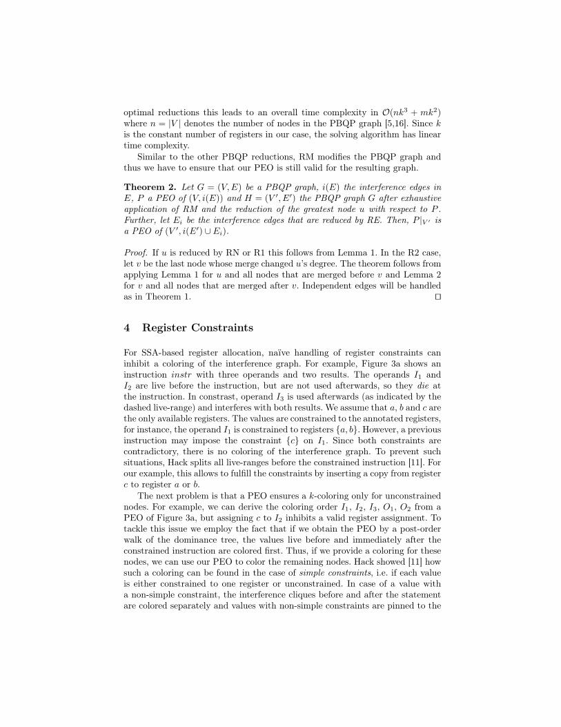
Theorem 2. Let G = (V,E) be a PBQP graph, i(E) the interference edges inE, P a PEO of (V, i(E)) and H = (V ′, E′) the PBQP graph G after exhaustiveapplication of RM and the reduction of the greatest node u with respect to P .Further, let Ei be the interference edges that are reduced by RE. Then, P |V ′ isa PEO of (V ′, i(E′) ∪ Ei).

Proof. If u is reduced by RN or R1 this follows from Lemma 1. In the R2 case,let v be the last node whose merge changed u’s degree. The theorem follows fromapplying Lemma 1 for u and all nodes that are merged before v and Lemma 2for v and all nodes that are merged after v. Independent edges will be handledas in Theorem 1. ut

4 Register Constraints

For SSA-based register allocation, naïve handling of register constraints caninhibit a coloring of the interference graph. For example, Figure 3a shows aninstruction instr with three operands and two results. The operands I1 andI2 are live before the instruction, but are not used afterwards, so they die atthe instruction. In constrast, operand I3 is used afterwards (as indicated by thedashed live-range) and interferes with both results. We assume that a, b and c arethe only available registers. The values are constrained to the annotated registers,for instance, the operand I1 is constrained to registers {a, b}. However, a previousinstruction may impose the constraint {c} on I1. Since both constraints arecontradictory, there is no coloring of the interference graph. To prevent suchsituations, Hack splits all live-ranges before the constrained instruction [11]. Forour example, this allows to fulfill the constraints by inserting a copy from registerc to register a or b.

The next problem is that a PEO ensures a k-coloring only for unconstrainednodes. For example, we can derive the coloring order I1, I2, I3, O1, O2 from aPEO of Figure 3a, but assigning c to I2 inhibits a valid register assignment. Totackle this issue we employ the fact that if we obtain the PEO by a post-orderwalk of the dominance tree, the values live before and immediately after theconstrained instruction are colored first. Thus, if we provide a coloring for thesenodes, we can use our PEO to color the remaining nodes. Hack showed [11] howsuch a coloring can be found in the case of simple constraints, i.e. if each valueis either constrained to one register or unconstrained. In case of a value witha non-simple constraint, the interference cliques before and after the statementare colored separately and values with non-simple constraints are pinned to the

chosen color. This may increase the register demand, but ensures a valid registerallocation.

Simple constraints can easily be integrated into the PBQP solving algorithm,since we only have to ensure that operands which are live after the constrainedinstruction are colored first. However, pinning the values to a single register isvery restrictive. In the following, we assume that the spiller enables a coloringby inserting possibly necessary copies of operands and present an algorithm thatcan deal with hierarchic constraints.

Definition 1 (hierarchic constraints). Let C be a set of register constraints.C is hierarchic if for all constraints C1 ∈ C and C2 ∈ C holds:

C1 ∩ C2 6= ∅ ⇒ C1 ⊆ C2 ∨ C2 ⊆ C1.

This definition excludes “partially overlapping” constraints, like C1 = {a, b}and C2 = {b, c}. As a result, the constraints form a tree with respect to strictinclusion, which we call constraint hierarchy. For instance, the constraint hi-erarchy for the general purpose registers of the IA-32 architecture consists ofCall = {A,B,C,D, SI,DI}, a subset Cs = {A,B,C,D} for instructions on 8-or 16-bit subregisters, and all constraints that consist of a single register.

For hierarchic constraints we obtain a valid register assignment of an inter-ference clique by successively coloring a most constrained node. However, fora constrained instruction we also have to ensure that after coloring the values,which are live before an instruction instr, we still can color the values live afterinstr. In Figure 3a O1 and O2 are constrained to a and b, respectively, and thusc must be assigned to I3. Unfortunately, c may also be chosen for I2 accordingto its constraints, if it is colored before I3. To avoid such situations, we wantto modify the constraints in a way that forces the first two operands to use thesame registers as the results. This is done in three steps:

1. Add unconstrained pseudo operands/results until the register pressure equalsthe number of available registers.

2. Match results and dying operands to assign result constraints to the corre-sponding operand, if they are more restrictive.

3. Try to relax the introduced constraints of the previous step, to enable moreaffinities to be fulfilled.

The first step ensures that the number of dying operands and the number ofresults are equal, which is required by the second step. For our example inFigure 3a we have nothing to do, since the register pressure before and afterinstr is already equal to the number of available registers.

4.1 Restricting operands

We employ Algorithm 2 for the second step. The algorithm has two parameters:A multiset of input constraints and a multiset of output constraints. It iterativelypairs an input constraint with an output constraint. For this pairing we select

I1 I2 I3

instr

O1 O2

{a, b} {a, b, c} {a, b, c}

{a} {b}

(a) Constrained instruction.

I1 I2 I3

instr

O1 O2

{a} {b} {a, b, c}

{a} {b}

(b) Constraints after transferringresult constraints to operands.

I1 I2 I3

instr

O1 O2

{a, b, c} {a, b, c} {c}

{a} {b}

(c) Constraints after relaxation ofoperand constraints.

I1 I2 I3

instr

O1 O2

{a, b} {a, b, c} {c}

{a} {b}

(d) Final constraints for PBQPconstruction.

Fig. 3: Handling of constrained instructions.

a minimal constraint (with respect to inclusion) Cmin. Then we try to find aminimal partner Cpartner, which is a constraint of the other parameter such thatCmin ⊆ Cpartner. If Cmin is an output constraint we transfer the constraint tothe partner. It is not necessary to restrict output constraints, since the inputsare colored first and restrictions propagate from there.

For our example in Figure 3a the algorithm input is {I1, I2} and {O1, O2}.The constraints of O1 and O2 are both minimal. We assume that the functiongetMinimalElement chooses O1 and thus Cmin = {a}. Since O1 is a result,the corresponding partner must be an operand. We select the only minimalpartner I1 which leads to Cpartner = {a, b}. We now have our first match (I1, O1)and remove both values from the value sets. Since the result constraint is morerestrictive, we assign this constraint to the operand I1. In the next iteration we

Algorithm 2 Restricting constraints of input operands.1: procedure restrictInputs(Ins,Outs)2: C ← Ins ∪Outs3: while C 6= ∅ do4: Cmin ← getMinimalElement(C)5: Cpartner ← getMinimalPartner(C, Cmin)6: C ← C \ {Cmin, Cpartner}7: if Cpartner from Ins then8: assign Cmin to partner value

match I2 and O2 and restrict I2 to {b}. The resulting constraints are shown inFigure 3b. Due to the introduced restrictions, the dying operands have to usethe same registers as the results.

In the following, we prove that getMinimalPartner always finds a minimalpartner. Furthermore, we show that Algorithm 2 cannot restrict the operandsconstraints in a way that renders a coloring of the values, which are live beforethe instruction, impossible.

Theorem 3. Let G = (V = I ∪ O, E) a bipartite graph with I = {I1, . . . , In}and O = {O1, . . . , On}. Further, let R = {R1, . . . , Rn} be a set of colors (reg-isters) and constr : V → P(R) a function that assigns each node its feasiblecolors. Moreover, let c : v 7→ Rv ∈ constr(v) be a coloring of V that assigns eachcolor to exactly one element of I and one element of O. Let M ⊆ E be a perfectbipartite matching of G such that

{u, v} ∈M ⇒ c(u) = c(v).

Then, Algorithm 2 finds a perfect bipartite matching M ′ such that there is acoloring c′ : v 7→ R′

v ∈ constr(v) that assigns each color to exactly one elementof I and one element of O with

{u, v} ∈M ′ ⇒ c′(u) = c′(v).

Proof. We prove the theorem by induction on n. For n = 1 there is only oneperfect bipartite matching and since c(I1) = c(O1) ∈ (constr(I1) ∩ constr(O1))we have constr(I1) ⊆ constr(O1) or constr(O1) ⊆ constr(I1). Thus, Algorithm 2finds the perfect bipartite matching which can be colored by c′ = c.

For n > 1, without loss of generality, we can rename the nodes such that∀i : c(Ii) = c(Oi) and Algorithm 2 selects O1 as node with minimal constraints.If the algorithm selects I1 to be the minimal partner, we can remove I1 and O1

from the graph, the color c(I1) from the set of colors R and apply the inductionassumption.

In case the algorithm does not select I1 as minimal partner let Ip be theminimal partner. Our goal is to show that there is a coloring for

M ′′ = (M \ {{I1, O1}, {Ip, Op}}) ∪ {{I1, Op}, {Ip, O1}}

and then apply the induction assumption. To obtain such a coloring we considerthe corresponding constraints. Since O1 has minimal constraints and c(I1) =c(O1) ∈ (constr(I1) ∩ constr(O1)), we get constr(O1) ⊆ constr(I1). Further-more, we know that Ip is the minimal partner of O1 which means constr(O1) ⊆constr(Ip) by definition. Thus, we get ∅ 6= constr(O1) ⊆ (constr(I1)∩constr(Ip))and since Ip is the minimal partner of O1, we get constr(Ip) ⊆ constr(I1). Usingthese relations, we obtain

c(O1) ∈ constr(O1) ⊆ constr(Ip)

c(Op) = c(Ip) ∈ constr(Ip) ⊆ constr(I1).

Thus, c′′ = c[I1 7→ c(Op), Ip 7→ c(O1)] is a coloring for M ′′. We now remove{Ip, O1} from the graph and c′′(O1) from the set of colors R and apply theinduction assumption, resulting in a matching M ′′′ and a coloring c′′′. Since c′′′does not use the color c′′(O1), we can extend the matching M ′′′ to

M ′ =M ′′′ ∪ {Ip, O1}

and the corresponding coloring c′′′ to

c′(v) =

{c′′(O1) , v ∈ {Ip, O1}c′′′(v) , otherwise

so {u, v} ∈M ′ ⇒ c′(u) = c′(v) holds. ut

4.2 Relaxing constraints

The restriction of the operands ensures a feasible coloring. However, some of theoperands may now be more restricted than necessary, so the third step relaxestheir constraints again. For instance, in Figure 3b the operands I1 and I2 arepinned to register a and b, respectively, but assigning register b to I1 and registera to I2 is also feasible. To permit this additional solution, the constraints canbe relaxed to {a, b} for both operands. In the following, we provide some rulesthat modify the constraint hierarchy of the input operands in order to relaxthe previously restricted constraints. We introduce two predicates to determinewhether a rule is applicable or not.

Dying A node is dying if the live-range of the operand ends at the instruction.Its assigned register is available for result values.

Saturated A constraint C is saturated, if it contains as many registers |C| asthere are nodes, which must get one of those registers assigned |{I ∈ I |CI ⊆ C}|. This means, every register in C will be assigned in the end.

Figure 4 shows the transformation rules for constraint hierarchies. The rules areapplied greedily from left to right. A constraint Ci is underlined if it is saturated.Each constraint has a set of dying nodes Ii and a set of non-dying nodes Ij .

I1 I2

C1 C2

I1 ∪ I2

C1 ∪ C2

⇒

(a) Merging two saturated con-straints consisting of dying nodes.

I1 ∪ I2

C1

C2

I1

I2

C1

C2 C1 \ C2

⇒

(b) Restricting non-dying nodes dueto a saturated constraint.

I1

I2 ∪ I3

C1

C2

I1 ∪ I2

I3

C1

C2

⇒

(c) Moving dying nodes alongthe constraint hierarchy.

{I3}

{I1} {I2}

{a, b, c}

{a} {b}

{I3}

{I1, I2}

{a, b, c}

{a, b}

⇒4a

{I1, I2} {I3}

{a, b, c}

{a, b} {c}

⇒4b

{I1, I2}

{I3}

{a, b, c}

{c}

⇒4c

(d) Application of the transformation rules to relax the operand constraintsshown in Figure 3b.

Fig. 4: Rules to relax constraints and a usage example.

The rule shown in Figure 4a combines two saturated constraints that containonly dying nodes. Applying this rule to the constraint hierarchy of our examplein Figure 3b lifts the constraints of I1 and I2 to {a, b}. Since both values die, itis not important which one is assigned to register a and which one to register b.

We now apply the rule of Figure 4b. This rule removes registers from a nodeconstraint if we know that these registers are occupied by other nodes, i.e. theconstraints consisting of these registers are saturated. Reconsidering the exampleshown in Figure 4d, the nodes I1 and I2 can only be assigned to register a andb. Thus, I3 cannot be assigned to one of these registers and we remove themfrom the constraint of I3. The transformation removes all nodes from the upperconstraint. Usually, we delete such an empty node after reconnecting all childrento its parent, because an empty node serves no purpose and the removal mayenable further rule applications. However, since {a, b, c} is the root of our tree—holding only unconstrained nodes—we keep it.

Since we want to relax the constraints of dying nodes as much as possible, therule shown in Figure 4c moves dying nodes upwards in the constraint hierarchy.This is only allowed, if the constraint C1 does not contain non-dying nodes. Forour example of Figure 4d we relax the constraints of I1 and I2 further to {a, b, c}.This would be disallowed without the application of 4b, because a or b couldthen be assigned to I3, which would render a coloring of the results impossible.

4.3 Obtaining a coloring order

After exhaustive application of the transformation rules, we obtain an orderingof the constraints by a post-order traversal of the constraint hierarchy, so moreconstrained nodes are colored first. For example, in Figure 4d the node I3 mustbe colored first due to this order. Within each constraint of the hierarchy, theassociated values are further ordered with respect to a post-order traversal overthe original constraint hierarchy. The second traversal ensures that “over-relaxed”values, i.e. values with a constraint that is less restrictive than their originalconstraint, are colored first. For our example in Figure 4d this means that wehave to color I1 before I2, although their relaxed constraints are equal. The finalnode order is I3, I1, I2. For the PBQP, we intersect the original (Figure 3a)and the relaxed constraints (Figure 3c); resulting in the constraints shown inFigure 3d. We now have an order to color the values live immediately before theconstrained instruction. Likewise, we obtain an order for the results by coloringthe more constrained values first. Finally, we obtain a coloring order for thewhole PBQP graph by employing the PEO for the remaining (unconstrained)nodes. This order ensures that our PBQP solver finds a register assignment evenin presence of constrained instructions.

5 Evaluation

In this section we evaluate the impact of our adaptations. First, the late decisionis compared to early decision making. Also, we investigate the effects of RM.

RM disabled RM enabled

Reduction Applications Ratio Applications Ratio

R0 2,047,038 — 2,013,003 —RE 126,002 — 33,759 —R1 106,828 13.9% 94,529 11.9%R2 363,221 47.2% 382,705 48.0%RN 298,928 38.9% 292,872 36.7%RM 0.0% 26,850 3.4%

Table 1: Percentages of reduction types.

Finally, our approach is compared to the current libFirm allocator in terms ofspeed and result quality.

5.1 Early vs. late decision

As mentioned in Section 3.3 we implemented early decision as well as latedecision. We evaluated both approaches using the C programs of the SPECCINT2000 benchmark suite. The programs compiled with late decision do notreach the performance of the programs compiled with early decision for anybenchmark, showing a slowdown of 3.9% on average. Especially the 253.perlbmkbenchmark performs nearly 20% slower.

We think that the quality gap stems from the different handling of affinities.An early decision takes account of the surrounding affinity costs and propagatesthem during the reduction. For a late decision a node and incident affinity edgesare removed from the PBQP graph first; then the decisions at adjacent nodesare made without accounting the affinity costs. When the late decision is made,the affinities may not be fulfilled due to decisions at interference neighbors thatwere not aware of these affinities.

5.2 Effects of RM

We added RM to our PBQP solver and Table 1 shows that 3.4% of the PBQPreductions during a SPEC compilation are RM. The number of nodes, remainingafter the graph is completely reduced, is given in the R0 row, but technicallythese nodes are not “reduced” by the solver, so they are excluded from the ratiocalculation. RE is also excluded, since it reduces edges instead of nodes. Theheuristic RN makes up 36.7% of the reductions, so these decisions are significant.The number of independent edge reductions decreases to nearly a fourth intotal, which suggests that a significant number of RE stem from nodes, whoseassignment is determined by a heuristic reduction of a neighbor. In case of RM,those edges are “redirected” to this neighbor instead. Another effect is that thenumber of heuristic decisions decreases by 2%. This reflects nodes that can be

Benchmark Recoloring PBQP Ratio

164.gzip 345 350 101.4%175.vpr 446 444 99.7%176.gcc 179 179 99.8%181.mcf 336 335 99.6%186.crafty 233 231 99.4%197.parser 468 467 99.7%253.perlbmk 355 354 99.8%254.gap 252 253 100.4%255.vortex 417 418 100.1%256.bzip2 374 371 99.4%300.twolf 684 680 99.4%

Average 99.9%

Table 2: Comparison of execution time in seconds with recoloring and PBQP.

optimally reduced after merging the neighbors into them. Altogether, the costsof the PBQP solutions decreased by nearly 1% on average, which shows thatRM successfully improved the heuristic decisions.

5.3 Speed evaluation

To evaluate the speed of the compilation process with PBQP-based copy co-alescing, we compare our approach to the recoloring approach [12]. Both ap-proaches are implemented within the libFirm compiler backend, so all otheroptimizations are identical. The SPEC CINT2000 programs ran on an 1.60GHzIntel Atom 330 processor on top of an Ubuntu 10.04.1 system. We timed the rele-vant phases within both register allocators and compare the total time taken fora compilation of all benchmark programs. The recoloring approach uses 11.6 sec-onds for coloring and 27.3 seconds for copy coalescing, which is 38.9 seconds intotal. In contrast, the PBQP approach integrates copy coalescing into the col-oring, so the coloring time equals the total time. Here, the total time amountsto 31.5 seconds, which means it takes 7.4 seconds less. Effectively, register as-signment and copy coalescing are 19% faster when using the PBQP approachinstead of recoloring.

5.4 Quality evaluation

To evaluate the quality of our approach, we compare the best execution timeout of five runs of the SPEC CPU2000 benchmark programs with the recoloringapproach. The results in Table 2 show a slight improvement of 0.1% on average.

In addition, we assess the quality of our copy minimization approach bycounting the inserted copies due to unfulfilled register affinities. We instrumentedthe Valgrind tool [15] to count these instructions during a SPEC run. Despite

PBQP Recoloring Ratio

Benchmark Instr. Swaps Copies Instr. Swaps Copies Swaps Copies

164.gzip 332 3.14% 0.71% 326 2.01% 0.19% 156.2% 374.7%175.vpr 202 4.38% 0.29% 201 4.32% 0.25% 101.4% 113.8%176.gcc 165 4.20% 0.30% 165 3.95% 0.28% 106.4% 108.9%181.mcf 50 4.22% 0.00% 50 4.72% 0.00% 89.4% 1047207.5%186.crafty 208 8.14% 0.56% 209 8.36% 0.64% 97.4% 87.7%197.parser 365 4.13% 0.56% 366 4.48% 0.28% 92.2% 198.5%253.perlbmk 396 4.64% 0.28% 408 5.97% 0.14% 77.7% 202.1%254.gap 259 7.02% 0.08% 259 6.86% 0.40% 102.4% 20.1%255.vortex 379 3.08% 0.53% 377 3.12% 0.16% 98.9% 339.2%256.bzip2 295 6.30% 0.14% 298 6.15% 0.93% 102.4% 14.9%300.twolf 306 4.80% 0.90% 306 4.33% 1.30% 110.6% 69.1%

Average 269 4.91% 0.40% 269 4.93% 0.42% 99.6% 95.2%

Table 3: Dynamic copy instructions in a SPEC run (in billions).

dynamic measuring, the results in Table 3 are static, because the input of thebenchmark programs is static. Since the number of instructions varies betweenprograms, we examine the percentage of copies. We observe that nearly 5% of theexecuted instructions are swaps and around 0.4% are copies on average. Becauseof the small number of copies a difference seems much higher, which results inthe seemingly dramatic increase of 1047208% swaps for 181.mcf. On average thepercentages decrease by 0.4% and 4.8%, respectively.

6 Future Work

Some architectures feature irregularities which are not considered in the contextof SSA-based register allocation. The PBQP has been successfully used to modela wide range of these irregularities by appropriate cost matrices [16]. While themodelling can be adopted for SSA-based register assignment, guaranteeing apolynomial time solution is still an open problem.

7 Conclusion

This work combines SSA-based with PBQP-based register allocation and in-tegrates copy coalescing into the assignment process. We introduced a novelPBQP reduction, which improves the quality of the heuristic decisions by merg-ing nodes. Additionally, we presented a technique to handle hierarchic registerconstraints, which enables a wider range of options within the PBQP. Our im-plementation achieves an improvement over the SSA-based recoloring approach.On average, the relative number of swap and copy instructions for the SPEC

CINT2000 benchmark was reduced to 99.6% and 95.2%, respectively, while tak-ing 19% less time for assignment and coalescing.

References

1. Bouchez, F., Darte, A., Rastello, F.: On the complexity of register coalescing. In:CGO ’07: Proceedings of the International Symposium on Code Generation andOptimization. pp. 102–114 (2007)

2. Braun, M., Mallon, C., Hack, S.: Preference-guided register assignment. In: Com-piler Construction, Lecture Notes in Computer Science, vol. 6011, chap. 12, pp.205–223. Springer Berlin / Heidelberg (2010)

3. Briggs, P., Cooper, K.D., Torczon, L.: Improvements to graph coloring registerallocation. ACM Trans. Program. Lang. Syst. 16(3), 428–455 (May 1994)

4. Brisk, P., Dabiri, F., Macbeth, J., Sarrafzadeh, M.: Polynomial time graph coloringregister allocation. In: 14th International Workshop on Logic and Synthesis. ACMPress (2005)

5. Buchwald, S., Zwinkau, A.: Instruction selection by graph transformation. In: Pro-ceedings of the 2010 international conference on Compilers, architectures and syn-thesis for embedded systems. pp. 31–40. CASES ’10, ACM, New York, NY, USA(2010)

6. Chaitin, G.J., Auslander, M.A., Chandra, A.K., Cocke, J., Hopkins, M.E., Mark-stein, P.W.: Register allocation via coloring. Computer Languages 6(1), 47–57(1981)

7. Dirac, G.: On rigid circuit graphs. Abhandlungen aus dem Mathematischen Semi-nar der Universität Hamburg 25, 71–76 (1961)

8. Ebner, D., Brandner, F., Scholz, B., Krall, A., Wiedermann, P., Kadlec, A.: Gen-eralized instruction selection using SSA-graphs. In: LCTES ’08: Proceedings of the2008 ACM SIGPLAN-SIGBED conference on Languages, compilers, and tools forembedded systems. pp. 31–40. ACM, New York, NY, USA (2008)

9. Eckstein, E., König, O., Scholz, B.: Code instruction selection based on SSA-graphs.In: Software and Compilers for Embedded Systems, Lecture Notes in ComputerScience, vol. 2826, pp. 49–65. Springer Berlin / Heidelberg (2003)

10. Grund, D., Hack, S.: A fast cutting-plane algorithm for optimal coalescing. In:Compiler Construction, chap. 8, pp. 111–125. Lecture Notes in Computer Science,Springer Berlin / Heidelberg (2007)

11. Hack, S.: Register allocation for programs in SSA form. Ph.D. thesis, UniversitätKarlsruhe (October 2007)

12. Hack, S., Goos, G.: Copy coalescing by graph recoloring. In: PLDI ’08: Proceedingsof the 2008 ACM SIGPLAN conference on Programming language design andimplementation (2008)

13. Hack, S., Grund, D., Goos, G.: Register allocation for programs in SSA-form. In:Compiler Construction, Lecture Notes in Computer Science, vol. 3923, pp. 247–262.Springer Berlin / Heidelberg (2006)

14. Hames, L., Scholz, B.: Nearly optimal register allocation with PBQP. In: ModularProgramming Languages, Lecture Notes in Computer Science, vol. 4228, chap. 21,pp. 346–361. Springer Berlin / Heidelberg (2006)

15. Nethercote, N., Seward, J.: Valgrind: a framework for heavyweight dynamic binaryinstrumentation. SIGPLAN Not. 42(6), 89–100 (June 2007)

16. Scholz, B., Eckstein, E.: Register allocation for irregular architectures. In: LCTES-SCOPES. pp. 139–148 (2002)